DYNA NON LINE - CAELinuxWikicaelinux.org/wiki/images/2/28/Pendulum_tutorial.pdf · ·...

DYNA_NON_LINEwith

Code Aster®A short introduction to using DYNA_NON_LINE to simulate a two segment pendulum.

For CAELinux.com, Feb. 2011 - Claus AndersenRev. 1.1

Pendulum tutorial for CAELinux.com � 2011

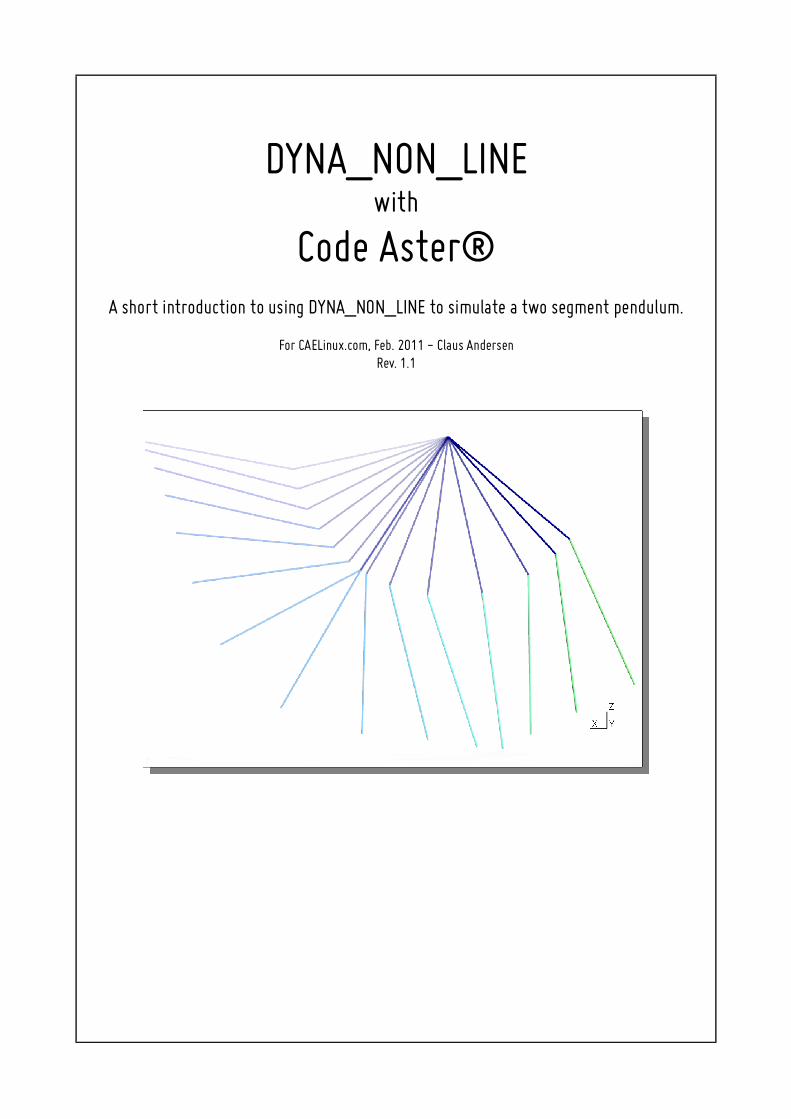
� Table of Contents

1 Prerequisites.....................................................................................................................3 2 Introduction.......................................................................................................................3 3 Setup................................................................................................................................4 4 Mesh.................................................................................................................................5 5 The .comm file..................................................................................................................6 6 Integrated post processing.............................................................................................10 7 Setting up ASTK.............................................................................................................17 8 (Important) notes when using DYNA_NON_LINE..........................................................19

8.1 Dampening..............................................................................................................19 9 Conclusion, remarks and author(s)................................................................................21 10 Links.............................................................................................................................22

2 of 22Published as GPL � rev. 1.1 - 29. Mar. 2011


1 Prerequisites

1 Prerequisites

� Working Code Aster® 10.2 or 10.3 � stable release. Stand-alone, SaloméMECA® version may not work with XMGrace®

� XMGrace® installed and working� Salomé (MECA)® or GMSH® for post-processing� User must be able to set up a simple job in ASTK®

2 Introduction

I've expanded the test-case SDNL100a (V5.02.100-1) to have two segments, and while theres really nothing to this simulation, I'll describe some of the discoveries I've made while setting it up.The simulation shows a two segment pendulum that swings under the influence of gravity.



3 Setup

3 Setup

The setup shown above, is two elements modelized as cables (MODE=CABLE). The reason for using a cable modelization, is that it is the modelization in Aster that, as far as I know, offers the greatest displacement and rotation without detecting a singular matrix (pivoting).

However, while cable elements are primed for great displacement and rotation, very small time steps must be used, and a generous value for the pivot detection (NPREC under SOLVEUR) has to be applied � more on this later.

Cable elements only have three degrees of freedom (DOFs), dx, dy ,dz. This means that however hard you try, you can only attach them as hinges � this also means that you can't impose a bending moment on them, and only 'normal stress' can be calculated for them (tension only, no compressive force). This is fine, because we want them to act as a hinged connection in this simulation.

Slightly relevant facts:

Beams (POUTRE) can be hinged as a boundary condition by omitting drx,dry,drz, but

NOT hinged together � they will act as if welded together as soon as you connect two or

more together.

Bars (BARRE) have the same properties as cables, except they are able to deal with

compressive forces.


Illustration A: The pendulum setup

X

Z N1 N2 N3

g


4 Mesh

4 Mesh

While I'm usually a big fan of the '.med' file format, I've had some problems using it for simulations involving very few (<5) elements, so in this case I've opted to use the native Code Aster® file format '.mail'

The native Code Aster® mesh format is very intuitive and it is not a problem to edit it by hand when we're only dealing with a handful of elements:

As seen above, the layout of the file is very straightforward; Coordinates for each of the three nodes, what element is connected to which nodes, and finally, which elements belong to the element group 'CABLE'

Instead of creating group names for each node and element, we'll just refer to them directly in the command file, since there are so few of them to chose from.


TITRE Pendulum tutorial

FINSFCOOR_3D

N1 0.00 0. 0. N2 1.00 0. 0.

N3 2.00 0. 0.FINSF

SEG2 NOM=CAB S1 N1 N2

S2 N2 N3FINSF

GROUP_MA NOM=CABLE S1

S2FINSF

FIN


5 The .comm file

5 The .comm file

---

Mesh=LIRE_MAILLAGE(FORMAT='ASTER',);

Model=AFFE_MODELE(MAILLAGE=Mesh,

AFFE=_F(GROUP_MA='CABLE',

PHENOMENE='MECANIQUE',

MODELISATION='CABLE',),);

---

Here we tell Aster to read the mesh file and name the concept 'Mesh', furthermore we assign a mechanical finite element model to the group 'CABLE', and name the concept 'Model'.

---

Material=DEFI_MATERIAU(ELAS=_F(E=100000000.0,

NU=0.0,

RHO=1.0,),

CABLE=_F(EC_SUR_E=1.0,),);

AssgnMat=AFFE_MATERIAU(MAILLAGE=Mesh,

AFFE=_F(TOUT='OUI',

MATER=Material,),);

---

Material properties are now defined � elasticity (Young's) module, Poisson's ratio and density.A special property for cables is needed here: EC_SUR_E defines how much the cable contracts radially when tension is applied to it.

The material properties just defined, is then assigned to every element (TOUT = OUI / all = yes)



5 The .comm file

---

Boundary=AFFE_CHAR_MECA(MODELE=Model,

DDL_IMPO=(_F(NOEUD='N1',

DX=0.0,

DY=0.0,

DZ=0.0,),

_F(NOEUD=('N2','N3',),

DY=0.0,),),);

Load=AFFE_CHAR_MECA(MODELE=Model,

PESANTEUR=_F(GRAVITE=9.81,

DIRECTION=(0.0,0.0,-1.0,),),);

---

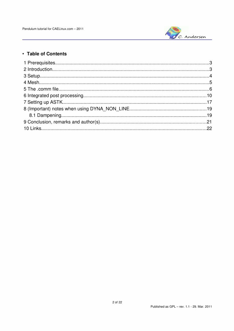
Assigning boundary conditions and loads.Node 1 is where the pendulum is attached, and therefore all the imposed degrees of freedom is set to zero, blocking all movement. In this case we're only working in the OXZ plane, so for the remaining two nodes, their movements in the Y direction are also restricted to zero.Notice we refer directly to the nodes with 'NOEUD' instead of using group names 'GROUP_NO'.

To get the pendulum swinging, we also need to apply gravity (PESANTEUR) to the model. A constant acceleration of 9.81 is applied in the Z-direction, to the entire model.

---

Characte=AFFE_CARA_ELEM(MODELE=Model,

CABLE=_F(GROUP_MA='CABLE',

SECTION=1.0,),);

---

Since the mesh describes one dimensional elements, some characteristics needs to be assigned to the cable elements. Naming the concept 'Characte' (damn the 8 character limit), assigning and describing a cable with a cross section of 1 to the group CABLE.

---



5 The .comm file

Listreel=DEFI_LIST_REEL(DEBUT=0.0,

INTERVALLE=_F(JUSQU_A=5.2,

NOMBRE=1040,),);

archive=DEFI_LIST_REEL(DEBUT=0.0,

INTERVALLE=_F(JUSQU_A=5.2,

NOMBRE=104,),);

---

Here a list of time steps for the calculation is generated. The calculation starts at 0.0s and ends at 5.2s and the calculation will be done in 1040 increments, effectively calculating the position of the pendulum at every (5.2s / 1040) 0.005s.

Since this will generate a lot of output to the temporary files on the hard-drive and won't be necessary for us to view a satisfactory result, a new list with only a 10th of the time steps are generated. This list will be used to inform the solver only to archive every 10th step.

Note: is it also possible to create time steps at every N up till 5.2s with the keyword PAS

instead of NOMBRE. So if you wanted a step at every 0.002s, you would end up with

(5.2 / 0.002) 2600 steps



5 The .comm file

---

RESU=DYNA_NON_LINE(MODELE=Model,

CHAM_MATER=AssgnMat,

CARA_ELEM=Characte,

EXCIT=(_F(CHARGE=Boundary,),

_F(CHARGE=Load,),),

COMP_ELAS=_F(RELATION='CABLE',

DEFORMATION='GROT_GDEP',),

INCREMENT=_F(LIST_INST=Listreel,

INST_INIT=0.,),

SCHEMA_TEMPS=_F(SCHEMA='NEWMARK',

FORMULATION='DEPLACEMENT',),

NEWTON=_F(REAC_ITER=1,),

CONVERGENCE=_F(RESI_GLOB_RELA=1.E-6,

ITER_GLOB_MAXI=20,),

ARCHIVAGE=_F(LIST_INST=archive,),);

---

� Create a non-linear dynamic concept and name it 'RESU'.� Use the finite element model assignment 'Model'� Include the assigned material 'AssgnMat'� Include the characteristics of the cables - 'Characte'� Include the two �excitation-concepts� - 'Boundary' and 'Load'� Use an elastic behavior for the cables (comportement = behavior), take great

rotations and displacements into account (GROT_GDEP)� Increment the calculation using the list previously created � 'Listreel' � start at

instant 0� Use the Newmark integration scheme (read more about this in U4.53.01 )� NEWTON: How the incremental calculation is solved (U4.51.03) � re-actualize

matrix at every iteration� CONVERGENCE: The global relative residuals must be lower than 1e-6 and there

can be a maximum of 100 iterations per time step, if the results are to be considered valid.

� Archive only the time steps corresponding to the list previously created - 'archive'

Note: There are literally thousands of pages describing each command/option � in French



5 The .comm file

� so I wont go into details here, to keep this tutorial relatively light. Look up their respective

User Documents (Ux.xx.xx)

---

IMPR_RESU(MODELE=Model,

FORMAT='MED',

RESU=_F(MAILLAGE=Mesh,

RESULTAT=RESU,

NOM_CHAM=('DEPL','ACCE','VITE',),),);

---

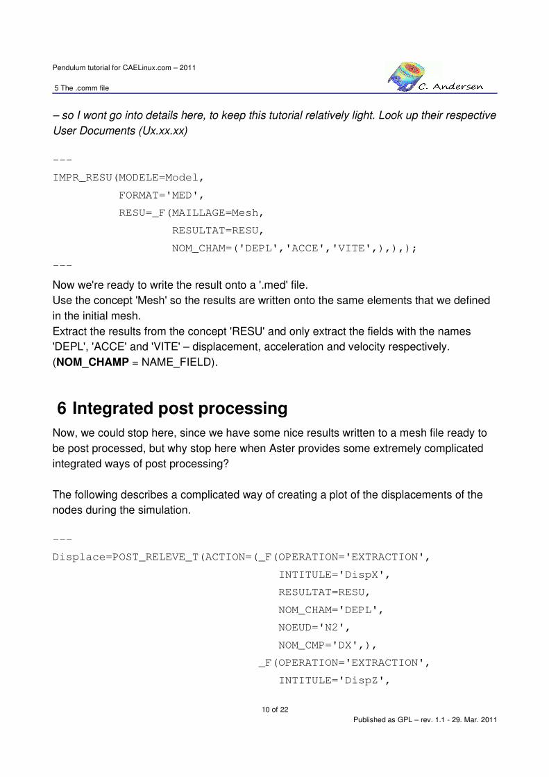
Now we're ready to write the result onto a '.med' file. Use the concept 'Mesh' so the results are written onto the same elements that we defined in the initial mesh.Extract the results from the concept 'RESU' and only extract the fields with the names 'DEPL', 'ACCE' and 'VITE' � displacement, acceleration and velocity respectively. (NOM_CHAMP = NAME_FIELD).

6 Integrated post processing

Now, we could stop here, since we have some nice results written to a mesh file ready to be post processed, but why stop here when Aster provides some extremely complicated integrated ways of post processing?

The following describes a complicated way of creating a plot of the displacements of the nodes during the simulation.

---

Displace=POST_RELEVE_T(ACTION=(_F(OPERATION='EXTRACTION',

INTITULE='DispX',

RESULTAT=RESU,

NOM_CHAM='DEPL',

NOEUD='N2',

NOM_CMP='DX',),

_F(OPERATION='EXTRACTION',

INTITULE='DispZ',




RESULTAT=RESU,

NOM_CHAM='DEPL',

NOEUD='N2',

NOM_CMP='DZ',),),);

---

Create a post processing concept (table) that extracts values and name it 'Displace'.Give the action the name 'DispX' (when e.g. printing to a table).Extract the values from the result 'RESU'. Specifically, obtain them from the field 'DEPL'.Only extract the values from node 2 and only extract the value for its movement (component) in the X-direction.

Now do the same for its movement in the Z-direction.

Note: POST_RELEVE_T is an incredibly powerful post processing tool that can calculate

average values over groups of nodes, resultants and moments of vectorial fields, trace

directions of fields and much much more, and output the result the tables � read more in

U4.81.21

Read about tracing curves with Code Aster® here: [U2.51.02] Tracé de courbes avec

Code Aster®---

DisX=RECU_FONCTION(TABLE=Displace,

PARA_X='INST',

PARA_Y='DX',);

DisZ=RECU_FONCTION(TABLE=Displace,

PARA_X='INST',

PARA_Y='DZ',);

T=RECU_FONCTION(TABLE=Displace,

PARA_X='INST',

PARA_Y='INST',);

---

'Recover' a function from the table 'Displace' just created and name it 'DisX'. For the X-axis use each instant � or time step. For the Y-axis use the component DX, i.e. the movement in the X-direction.




Do the same for a concept named 'DisZ'

'Recover' a function for 'time' to be used in the plot. The plotting tool needs a function for time and cannot extract INST (time steps) by itself, which is why we need to create this function.




---

IMPR_FONCTION(FORMAT='XMGRACE',

PILOTE='POSTSCRIPT',

UNITE=28,

COURBE=(_F(FONC_X=T,

FONC_Y=DisX,

LEGENDE='DispX',

COULEUR=2,

MARQUEUR=0,),

_F(FONC_X=T,

FONC_Y=DisZ,

LEGENDE='DispZ',

COULEUR=1,

MARQUEUR=0,),),

TITRE='Displacement of node N2',

GRILLE_X=0.001,

GRILLE_Y=0.001,

LEGENDE_X='[Sec]',

LEGENDE_Y='[Dist]',);

---

Print a function � use the format XMGrace® (the plotting tool)When XMGrace® writes the physical file, use the postscript file format. A variety of other formats exists as well, such as .png, .jpg, etc.Use the LU 28 (logic unit � a number used by Fortran to identify files, rather than using file names.). How ASTK® needs to be set up for this will be described later.

Now create a curve based on the two functions: 'T' for the X-axis and 'DisX' for the Y-axis.Give the curve the legend 'DispX', use the color 2 and no marker points on the curve (=0).

Do the same for the function 'DisZ'.

Give the plot the title 'Displacements of node N2'.Axis ticks of X and Y should be at 0.001 increments and respective axes should have the legend '[Sec]' and '[Dist]'.




Note: The values for e.g. color and marker can be found in U4.33.01, the IMPR_FONC

document.

Above chain of commands should print a plot similar to this:




The same is done for node 3 and then a plot that plots the DX movements against the DZ movements.The commands can be found in the .comm file and are not included here.Creates these two plots:



7 Setting up ASTK

7 Setting up ASTK

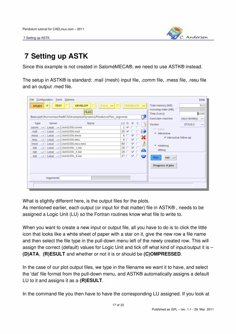
Since this example is not created in SaloméMECA®, we need to use ASTK® instead.

The setup in ASTK® is standard: .mail (mesh) input file, .comm file, .mess file, .resu file and an output .med file.

What is slightly different here, is the output files for the plots. As mentioned earlier, each output (or input for that matter) file in ASTK® , needs to be assigned a Logic Unit (LU) so the Fortran routines know what file to write to.

When you want to create a new input or output file, all you have to do is to click the little icon that looks like a white sheet of paper with a star on it, give the new row a file name and then select the file type in the pull-down menu left of the newly created row. This will assign the correct (default) values for Logic Unit and tick off what kind of input/output it is � (D)ATA, (R)ESULT and whether or not it is or should be (C)OMPRESSED.

In the case of our plot output files, we type in the filename we want it to have, and select the 'dat' file format from the pull-down menu, and ASTK® automatically assigns a default LU to it and assigns it as a (R)ESULT.

In the command file you then have to have the corresponding LU assigned. If you look at



7 Setting up ASTK

the command file you will see we have the keyword/value 'UNITE=28,' for the first plot file, and 29 and 27 for the subsequent files.

Since you've already created the input files, click the folder icon, find the file, and ASTK® will automatically detect what kind of file you're opening and assign the correct LU etc.

That is about what is needed to run this simulation. The simulation can easily be extended with more segments and/or 2D/3D elements.



8 (Important) notes when using DYNA_NON_LINE


Code Aster® should not be the first choice when it comes to simulating kinematics; it is simply built from the ground up over the last decade and more, to simulate civil, nuclear and mechanical engineering, with small stresses and strains, and no specific emphasis has (as far as I know) been put on simulating linkages, drop- and crash-tests etc. That is not to say that it can't be coaxed.

So, when working with cables in Code Aster®, it is very important to use incredibly small time steps compared to other types of studies, otherwise pivoting will be detected. Likewise it is advisable to set a relatively low number of maximum Newtons iterations per time step (DYNA_NON_LINE -> COVERGENCE -> ITER_GLOB_MAXI), otherwise the 'global residuals' (RESI_GLOB_MAXI) will skyrocket exponentially and error out.

As stated earlier, when using too large time steps, Code Aster® will detect a singular matrix (pivoting) and again, error out. This can however, be mitigated by increasing the value NPREC under DYNA_NON_LINE -> SOLVEUR, from the standard 8 digits, carefully.�NPREC tells the default linear solver (MULT_FRONT) to continue even if the solution of Ku=f was not precise (usually a sign of null pivot). That's why it is not recommended to use such a parameter since it can lead to a solution u which does not verify Ku=f� -Thomas De Soza

Working with cables and very small time steps can be frustrating, especially when using cables with other structures, where small time steps are required initially when the cables 'settle', but greater time steps can be used for the remainder of the calculation. It is therefore recommended to get familiarized with 'Automatic Time Stepping' as described in [U4.34.03] Opérateur DEFI_LIST_INST

8.1 Dampening

This pendulum will, if left alone, continue swinging forever and never come to a rest. This is because no (significant) dampening is introduced in the simulation. When the default integration scheme NEWMARK is used, small values for dampening BETA=0.25 and GAMMA=0.50 (trapezoidal rule) is indeed introduced. This is fine for most cases, but should the calculation become unstable, this can be increased to stabilize it.




It can also be increased intentionally, to let the pendulum come to a rest.

It can be illustrated by increasing BETA to 5 and GAMMA to 10, which in turn shows us diminishing oscillation in the following graph:

More on the integration schemes and their pros and cons, can be found in section 3.16 of U4.53.01.



9 Conclusion, remarks and author(s)

9 Conclusion, remarks and author(s)

That's it for this tutorial. Much more information can be found in the user documents on the Code Aster® website, its forum and on the CAELinux website.

Remark:Any and all information and content in this document is published under the GPL license and can as such be used or reproduced in any way. The author(s) only ask for acknowledgment in such an event.Acknowledgment goes out to EDF for releasing Code Aster® as free software and to all those who help out by answering questions in the forum and writing documentation / tutorials.Contributions and/or corrections to this tutorial are always welcomed.

Author(s):Claus Andersen � ClausAndersen81_[at]_gmail.com

ENDED OK



10 Links

10 Links

[CAELinux Website] www.caelinux.com[Code Aster® Website] www.code-aster.org

[GMSH® Website] www.geuz.org/GMSH[XMGrace® Website] http://plasma-gate.weizmann.ac.il/Grace/


DYNA NON LINE - CAELinuxWikicaelinux.org/wiki/images/2/28/Pendulum_tutorial.pdf · ·...

Documents

Transcript of DYNA NON LINE - CAELinuxWikicaelinux.org/wiki/images/2/28/Pendulum_tutorial.pdf · ·...