Dyalog APL R Interface Guide

The tool of thought for expert programming

Dyalog APL R

Interface Guide Version 1.1

Dyalog Limited

Minchens Court, Minchens Lane

Bramley, Hampshire

RG26 5BH

United Kingdom

tel: +44(0)1256 830030

fax: +44 (0)1256 830031

email: [email protected]

http://www.dyalog.com

Dyalog is a trademark of Dyalog Limited

Copyright 1982-2014

mailto:[email protected]

Copyright 2014 by Dyalog Limited.

All rights reserved.

Version 1.1

First Edition April 2015

Draft dated April 14th, 2015

No part of this publication may be reproduced in any form by any means without the

prior written permission of Dyalog Limited, Minchens Court,

Minchens Lane, Bramley, Hampshire, RG26 5BH, United Kingdom.

Dyalog Limited makes no representations or warranties with respect to the contents

hereof and specifically disclaims any implied warranties of merchantability or fitness for

any particular purpose. Dyalog Limited reserves the right to revise this publication

without notification.

All other trademarks and copyrights are acknowledged.

Contents

1 ABOUT THIS DOCUMENT . . . . . . . . . . . . . . . . . . . . . . . . . . . . . . . . . . . . . . . . . . . . . . . . . . . . . . . . . . . . . . 1 1.1 Changes since version 1.0 ................................................................................. 1

1.2 Limitations in RConnect 1.1 .............................................................................. 1

2 INTRODUCTION . . . . . . . . . . . . . . . . . . . . . . . . . . . . . . . . . . . . . . . . . . . . . . . . . . . . . . . . . . . . . . . . . . . . . . . . . . 2

3 A SAMPLE RCONNECT SE SSION . . . . . . . . . . . . . . . . . . . . . . . . . . . . . . . . . . . . . . . . . . . . . . . . . . . . . 3

4 INSTALLATION AND INI TIALISATION . . . . . . . . . . . . . . . . . . . . . . . . . . . . . . . . . . . . . . . . . . . . . . 6 4.1 Prerequisites ..................................................................................................... 6

4.2 Adding R to the Windows PATH environment variable .................................... 6

4.3 Installing R and rscproxy ................................................................................... 7

4.4 Packages ............................................................................................................ 7

4.5 Running RConnect ............................................................................................. 8

4.6 Accessing R's Documentation ........................................................................... 9

5 TRANSFERRING DATA BE TWEEN APL AND R . . . . . . . . . . . . . . . . . . . . . . . . . . . . . . . . . . 10 5.1 Compatible R Arrays and Lists ......................................................................... 10

5.2 R Objects ......................................................................................................... 10

5.3 R data.frame objects ....................................................................................... 11

5.4 Constructing R objects .................................................................................... 12

5.5 Letting R do the formatting ............................................................................. 13

6 RCONNECT FUNCTIONS . . . . . . . . . . . . . . . . . . . . . . . . . . . . . . . . . . . . . . . . . . . . . . . . . . . . . . . . . . . . . . 14 6.1 init ................................................................................................................... 14

6.2 save ................................................................................................................. 14

6.3 get ................................................................................................................... 15

6.4 put ................................................................................................................... 15

6.5 execute ............................................................................................................ 15

6.6 format ............................................................................................................. 16

7 MORE ABOUT RCONNECT OBJECTS . . . . . . . . . . . . . . . . . . . . . . . . . . . . . . . . . . . . . . . . . . . . . . 18 7.1 Robject and RDataframe ................................................................................. 18

7.1.1 Constructors .................................................................................................... 19

7.1.2 The Value property ......................................................................................... 19

7.1.3 The attributes property ................................................................................... 20

7.1.4 The attr property ............................................................................................. 20

7.1.5 Changing Class ................................................................................................. 21

7.2 Special Classes ................................................................................................. 21

7.2.1 Renvr ............................................................................................................... 21

7.2.2 Rname ............................................................................................................. 21

7.2.3 Rcall ................................................................................................................. 22

7.2.4 Rexpr ............................................................................................................... 22

7.2.5 Rfunc ............................................................................................................... 22

8 PERFORMANCE TIPS . . . . . . . . . . . . . . . . . . . . . . . . . . . . . . . . . . . . . . . . . . . . . . . . . . . . . . . . . . . . . . . . . . 24

APPENDIX A R FOR APLERS . . . . . . . . . . . . . . . . . . . . . . . . . . . . . . . . . . . . . . . . . . . . . . . . . . . . . . 25 A.1 Assignment and Vector Arithmetic ................................................................. 25

A.2 Operators ........................................................................................................ 26

A.3 Arrays .............................................................................................................. 27

A.4 Functions on Arrays......................................................................................... 28

A.5 Data Frames .................................................................................................... 29

A.6 Indexes ............................................................................................................ 30

A.7 Defined Functions ........................................................................................... 32

APPENDIX B REFERENCES FOR R . . . . . . . . . . . . . . . . . . . . . . . . . . . . . . . . . . . . . . . . . . . . . . . 34

Dyalog APL R Interface Guide

1 About This Document

This document describes how to install and use RConnect, the interface between Dyalog APL and R.

The information provided in this document is not a tutorial for R and does not include comprehensive information on the capabilities and syntax of R – only some basics are covered. See Appendix B for a list of suggested documentation and references that expand on this.

Dyalog only supports RConnect on Unicode editions of Dyalog APL. Version 1.1 requires Dyalog APL version 14.1, and is supported on Microsoft Windows, Linux and OS X.

RConnect is supported on the same levels of Windows, Linux and OS as Dyalog APL. However, some features of R are operating-system dependent, so may not work on your platform.

It is assumed that the reader has a reasonable understanding of Dyalog APL. No prior knowledge of R is required.

1.1 Changes since version 1.0

Support has been added for OS X (Yosemite 10.10.x)

The rscproxyLin class/driver has been renamed rscproxyUNIX to reflect support for both Linux and OS X

Rconnect will now generate an error if run under Classic Dyalog

Rconnect now works with R 3.1.2 on Windows

A number of minor bug fixes

The example in section 5.5 now works

1.2 Limitations in RConnect 1.1

RConnect is still work in progress, and a number of limitations still apply:

The R help system does not work on Linux or OS X; a browser window opens when help() is called, but the window is not populated with help text

Under Linux and OS X graphics windows are not resizable and cannot be closed. To close a graphics window call graphics.off()

Dyalog APL R Interface Guide 2

2 Introduction

R is an open-source integrated programming language and software environment for statistical computing and graphics. The R language is widely used among statisticians and data miners for developing statistical software and data analysis, and the popularity of R has increased substantially in recent years.

RConnect, the interface between Dyalog APL and R, makes the R environment an extension of the active APL workspace. With RConnect:

R functions can be called directly from within a Dyalog APL session, passing APL arrays as arguments and receiving APL arrays as results.

the contents of APL variables can be transferred to and from equivalent R variables.

simple R arrays and lists (without named items) can be converted directly to equivalent APL arrays.

the most widely used R classes, such as list (with named items), table, data.frame and ts (timeseries) can be converted to corresponding APL classes to make them easier to use from within the APL workspace.

R classes that are not directly supported in APL are encapsulated in an R.object class, making it possible to inspect and manipulate the attributes of the object from within the APL workspace.

RConnect enables APL users to extend APL applications by either utilising existing R skills or acquiring new skills and making use of the large – and rapidly expanding – collection of statistical and analytical packages that are continuously being added to R by existing users.


3 A Sample RConnect Session

This chapter comprises examples that provide an overview of the capabilities of the RConnect interface. It is assumed that R and any required packages have been installed – for details on how to perform the required installations, see section 4.1.

First, load the RConnect workspace:

)load rconnect rconnect saved Thu Mar 06 21:35:43 2015

The next step is to create an instance of the R class and initialise it. This is done in two steps, making it possible to set options before making the connection to R.

r←⎕NEW R r.init RConnect initialized

R expressions can now be executed using the function r.x. Results are returned as APL arrays. The result of r.x is shy, so the explicit ⎕← is required to display the output in the session.

⎕←r.x '1+2' ⍝ Add two scalars 3

⎕←r.x 'c(1,2,3)*c(10,20,30)' ⍝ Make & multiply 2 lists 10 40 90

⎕←r.x 'matrix(1:12,3)' ⍝ Matrix with 3 rows from 1:12 1 4 7 10 2 5 8 11 3 6 9 12

⎕←r.x 'matrix(1:12,3,byrow=TRUE)' ⍝ Row major as APL 1 2 3 4 5 6 7 8 9 10 11 12

So far this is nothing that could not be done (more easily) using APL. However, R's libraries of built-in statistical and analytical functions are enormous, starting with simple ones like:

⎕←r.x 'rnorm(10)' ¯1.201069489 0.3935029841 ¯0.3554851217 0.01064592962 1.29373234 ¯0.4275097121 ¯0.6812233687 0.5906630588 ¯0.5442389192 1.531940771

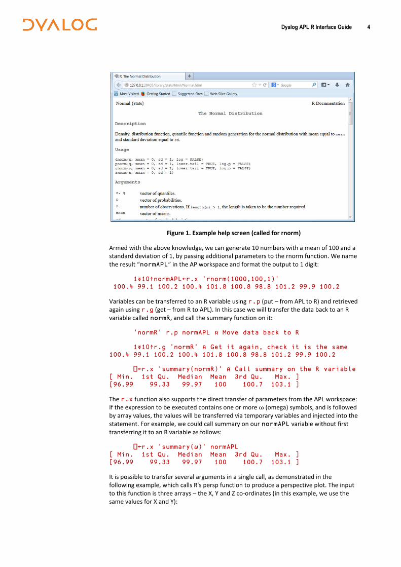
We can invoke R’s on-line help system by calling the help function:

r.x 'help(rnorm)'

The help will appear in the default browser as shown in Figure 1.


Figure 1. Example help screen (called for rnorm)

Armed with the above knowledge, we can generate 10 numbers with a mean of 100 and a standard deviation of 1, by passing additional parameters to the rnorm function. We name the result “normAPL” in the AP workspace and format the output to 1 digit:

1⍕10↑normAPL←r.x 'rnorm(1000,100,1)' 100.4 99.1 100.2 100.4 101.8 100.8 98.8 101.2 99.9 100.2

Variables can be transferred to an R variable using r.p (put – from APL to R) and retrieved again using r.g (get – from R to APL). In this case we will transfer the data back to an R variable called normR, and call the summary function on it:

'normR' r.p normAPL ⍝ Move data back to R

1⍕10↑r.g 'normR' ⍝ Get it again, check it is the same 100.4 99.1 100.2 100.4 101.8 100.8 98.8 101.2 99.9 100.2

⎕←r.x 'summary(normR)' ⍝ Call summary on the R variable [ Min. 1st Qu. Median Mean 3rd Qu. Max. ] [96.99 99.33 99.97 100 100.7 103.1 ]

The r.x function also supports the direct transfer of parameters from the APL workspace: If the expression to be executed contains one or more ⍵ (omega) symbols, and is followed by array values, the values will be transferred via temporary variables and injected into the statement. For example, we could call summary on our normAPL variable without first transferring it to an R variable as follows:

⎕←r.x 'summary(⍵)' normAPL [ Min. 1st Qu. Median Mean 3rd Qu. Max. ] [96.99 99.33 99.97 100 100.7 103.1 ]

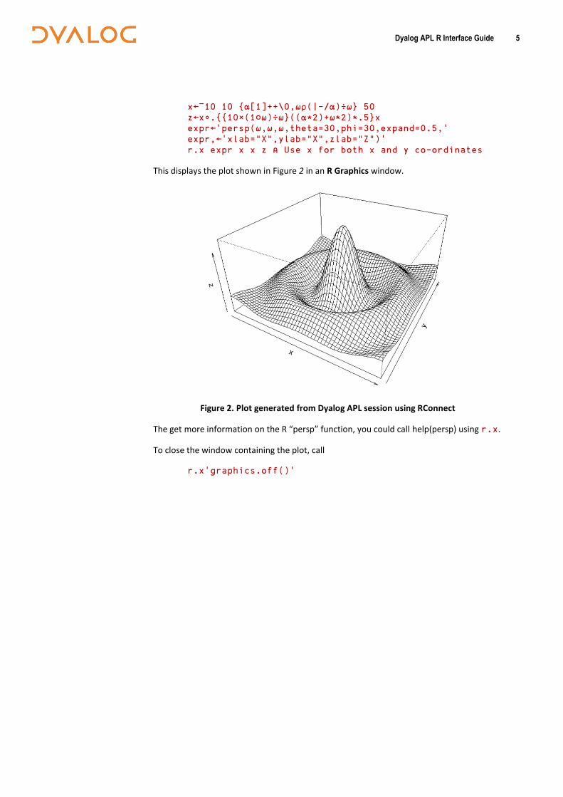
It is possible to transfer several arguments in a single call, as demonstrated in the following example, which calls R's persp function to produce a perspective plot. The input to this function is three arrays – the X, Y and Z co-ordinates (in this example, we use the same values for X and Y):


x←¯10 10 {⍺[1]++\0,⍵⍴(|-/⍺)÷⍵} 50 z←x∘.{{10×(1○⍵)÷⍵}((⍺*2)+⍵*2)*.5}x expr←'persp(⍵,⍵,⍵,theta=30,phi=30,expand=0.5,' expr,←'xlab="X",ylab="X",zlab="Z")' r.x expr x x z ⍝ Use x for both x and y co-ordinates

This displays the plot shown in Figure 2 in an R Graphics window.

Figure 2. Plot generated from Dyalog APL session using RConnect

The get more information on the R “persp” function, you could call help(persp) using r.x.

To close the window containing the plot, call

r.x'graphics.off()'


4 Installation and Initialisation

This chapter describes how to install and initialise R for use with RConnect.

4.1 Prerequisites

The following software must be installed prior to using RConnect 1.1:

Dyalog APL Unicode edition version 14.1

R version 3.1 or later (32-bit for user with 32-bit APL, 64-bit for 64-bit APL)

The rscproxy R package

The gtools R package is required by the r.f function

The examples used in the previous section make use of the rnorm function from the stats package and the persp function from the graphics package.

On OS X the RConnect workspace requires otool in order to locate the various R files. otool is not part of the standard OS X installation; type otool in a command window for more information on installing this command

4.2 Adding R to the Windows PATH environment variable

On Windows it is necessary to add the R binary file directory to the system environment variable PATH. Remember that this will need to be updated if a new version of R is installed. There have been reports that it has been necessary to add the PATH variable (with the R directories included) to the user environment variable too.

To add R to the path on Windows:

1. Open the Control Panel and select System.

2. Under Control Panel Home, select Advanced system settings. The System Properties window is displayed.

3. Navigate to the Advanced tab and click Environment Variables….

4. In the System variables list, select the Path variable and click Edit….

5. Add <path to R>\bin\i386 (and/or x64) to the beginning of the Variable value (unless it is already present in the path) and click OK. Include the trailing “\”and include the path separator, “;”.

Typically the path to R is C:\Program Files\R\R-3.1.3\bin\x64\


4.3 Installing R and rscproxy

R is included in a number of Linux distributions so can be installed using the Linux package manager included in your distribution. For Windows, OS X and other Linux distributions R can be downloaded from http://www.r-project.org/. Full installation instructions are included on this website.

To install rscproxy:

1. Start R. If R is started with administrator/root/super user privileges it will be possible to install rscproxy into the system R packages area. If run without such privileges rscproxy will have to be installed in a user packages area.

Linux start a console window and run R

Windows: double click on the R shortcut

OS X: either click on the R application or open a command window and type R

2. on OS X it is recommended to set the language to en_US.UTF-8 system("defaults write

org.R-project.R force.LANG en_US.UTF-8")

3. Run install.packages("rscproxy")

and follow the instructions.

Note: when copying and pasting the above instruction(s) ensure that the quotes entered into R are double quotes, not smart quotes !

4. Run install.packages()

to check that rscproxy is included in the list

4.4 Packages

A core set of packages is installed with R. These comprise a basic set of abilities, datasets and standard statistical and graphical functions. Additional packages that extend R's capabilities through more specialised statistical techniques, graphical devices, reporting tools and so on, can be downloaded from various repositories, including:

The Comprehensive R Archive Network: http://cran.r-project.org/

Crantastic http://crantastic.org/packages (a community site for R packages that includes user reviews)

The Omega Project for Statistical Computing: http://www.omegahat.org/

Bioconductor: http://www.bioconductor.org/packages/release/ (packages for analysis/comprehension of high-throughput genomic data)

http://www.r-project.org/

http://cran.r-project.org/

http://crantastic.org/packages

http://www.omegahat.org/

http://www.bioconductor.org/packages/release/


Once a package has been downloaded and installed it needs to be loaded using the library() command before it can be used by R.

Various R commands can be entered in the R Console (within the R user interface) to manipulate packages. A few examples are listed below, see the R documentation for more information.

library() lists the contents of the <path to R>\library directory (the installed packages)

library(<package name>) loads the specified package

install.packages('<package name>')

downloads and installs the specified package from the Comprehensive R Archive Network (http://cran.r-project.org/)

update.packages('<package name>')

updates the specified package from the Comprehensive R Archive Network (http://cran.r-project.org/)

search() lists the packages that are currently loaded

help(package="<package name>") opens the online help information for the specified package

4.5 Running RConnect

1. Start Dyalog APL.

2. Copy or load the rconnect workspace: )load rconnect

3. Create a new instance of the R class:

r←⎕NEW R

Throughout this document, r is used to denote an instance of the R class.

4. Establish the connection to R: r.init RConnect initialized

5. If step (4) fails, it will be necessary to explicitly set the path to the driver that will be used before calling r.init: on Windows: r.setdriver 'rscproxyWin' '<path>\R\R-<vn>\'

on Linux or OS X




r.setdriver 'rscproxyUNIX' '<path>/R/R-<vn>/'

The functions r.save, g.g, r.p, r.x and r.f can now be used (see Chapter 6).

Although instances or the R object can be saved in an APL workspace, the connection to R is broken if the workspace is saved and reloaded. This means that the connection to R needs to be re-established by calling the r.init function each time the workspace is loaded. If the r.save function has been used (see Section 6.2), then the initialisation also restores the previous R session's state (for example, variables).

4.6 Accessing R's Documentation

R has online documentation that, once enabled, should be able to be opened from within an APL session using the help(...) function; calling this function should result in a browser window being opened which displays the relevant help text.

On UNIX-based operating systems this does not currently work.


5 Transferring Data between APL and R

5.1 Compatible R Arrays and Lists

Many values returned to APL by r.x or r.g are R structures which have a direct equivalent in APL. In particular, many instances of the R list and array classes can be converted to APL arrays:

A list in R maps to a nested array in APL In R, a list is a vector of elements each of which can contain any type of R object and,

optionally a names (item names) attribute.

An array in R maps to a simple array in APL In R, an array is a vector of elements with attributes dim (dimensions) and, optionally,

dimnames (dimension names).

The mapping to APL arrays is only possible if the R list has no item names, and an R array has no dimension names. R lists and arrays with additional attributes, and all other R classes, are mapped to instances of the Robject or Rdataframe classes, which are described in the next section.

Numeric types, including booleans and complex numbers are converted as one would expect, and R strings are converted to enclosed character vectors. R strings are converted to enclosed character vectors.

R does not support the decimal floating point: RConnect converts these into double precision floating point types when transferring them from an APL session into an R session. This conversion can fail if the values are outside the range of double precision floating point, and a loss of precision is also possible. Values will remain as double precision floating point types when transferred back to the APL session.

R has a richer set of values used for missing or invalid values, for which there is no exact equivalent in APL: The R constants NULL (missing value), NA (not available), NaN (not a

number) and Inf (infinity) are all converted to ⎕NULL in APL. On the reverse journey, all

⎕NULLs are converted to NA.

5.2 R Objects

R is a rather loosely organised “object-oriented” system, where variables can have attributes and one of the attributes is called class. The R language does not enforce any relationship between class and the set of attributes that an object has, but the behaviour of much of the R framework is driven by conventions associated with the attributes that an object of a particular class is expected to have.

RConnect considers all objects to be instances of the same Robject class. For example let use retrieve and examine “co2”, a sample dataset included with R, which contains monthly data from 1959 to 1997 – this is an R object with class “ts”:


⎕CLASS co2←r.g 'co2' ⍝ The APL class is: #.Robject

⎕←co2 ⍝ Default display form [R ts - 468 observations] Frequency 12 Start 1959 1 End 1997 12

The Robject class has three properties that can be used to get at the contents (or modify them): attributes is a 2-column matrix containing attribute names and values: co2.attributes ⍝ List attributes and values class ts tsp 1959 1997.916667 12

There is a keyed property called attr which can be used to extract values of named attributes:

co2.attr[⊂'tsp'] ⍝ Extract one attribute value 1959 1997.916667 12

Finally, the Value property contains the data:

8↑co2.Value 315.42 316.31 316.5 317.56 318.13 318 316.39 314.65

The Value property is also the default property, which means that the object can be indexed directly, and the entire contents can be produced using monadic ⌷:

co2[2 4 6] 316.31 317.56 318

⍴⌷co2 468

As we have just seen, the ts class is one of several commonly used R classes that RConnect recognises, and attempts to set a useful default display format. We saw another example of RConnect providing formatting when we used the summary function in the previous section: RConnect recognised that the result is a special kind of table object named summaryDefault and set the display form to be something similar to what R itself would have displayed:

⎕←r.x 'summary(⍵)' normAPL [ Min. 1st Qu. Median Mean 3rd Qu. Max. ] [96.99 99.33 99.97 100 100.7 103.1 ]

The set of R classes that APL provides special formatting for will probably continue to grow as more cases where RConnect could help with the display of R objects in APL are discovered. Please contact [email protected] if you would like to suggest a display form for a frequently-used R class.

5.3 R data.frame objects

A very common data type used by R is the data.frame, which is accepted as input by many of the statistical functions. RConnect converts data.frame values to instances of



Rdataframe, a class which has the same properties as Robject – the main difference being that the Value property is a matrix with one column per data series:

The following example show the construction (using R language statements) and the display of a data.frame. Note that R also uses the assignment arrow, but unlike APL spells it using two symbols, “<-“:

r.x 'age <- 18:20' ⍝ Generate ages in R r.x 'height <- ⍵' (76.1 77 78.1) ⍝ heights from APL r.x 'village <- data.frame(age=age,height=height)' ⎕←v←r.g 'village' ⍝ Display the data.frame in APL [R data.frame - 3 rows] age height 18 76.1 19 77 20 78.1

v.attributes ⍝ display with ]boxing on ┌─────────┬────────────┐ │class │data.frame │ ├─────────┼────────────┤ │row.names│1 2 3 │ ├─────────┼────────────┤ │names │┌───┬──────┐│ │ ││age│height││ │ │└───┴──────┘│ └─────────┴────────────┘

v.Value 18 76.1 19 77 20 78.1

5.4 Constructing R objects

Because R objects all have the same general structure, you can manufacture any R object from APL by setting the correct attributes – one of which will be the R the class name. R attribute names are R strings (enclosed character vectors in APL), and attribute values can be any R object.

Be careful: RConnect does very little validation of the attribute names and values: you can probably cause crashes in R functions if you do not adhere to the expected conventions, which you can only learn about by reading the documentation for each class or function.

The following example creates an R object of class ts:, containing one year of monthly data. The tsp property is expected to contain the start and end dates, and the frequency:

tsp←2014 (2014+11÷12) 12 ⍝ From month 0 to 11 of 2014 attributes←2 2⍴'class' 'ts', 'tsp' tsp value←?12⍴100 myts←⎕NEW Robject (value attributes)

'myts' r.p myts

r.f 'myts' Jan Feb Mar Apr May Jun Jul Aug Sep Oct Nov Dec 2014 53 10 66 42 71 92 77 27 5 74 33 64


⎕←r.x 'summary(myts)' [ Min. 1st Qu. Median Mean 3rd Qu. Max. ] [ 5 31.5 58.5 51.17 71.75 92 ]

The same is possible for data.frame objects:

names←'names' ('xx' 'square')

mydf←⎕NEW Rdataframe (((⍳12)∘.*1 2) names) 'mydf'r.p mydf

⎕←r.x 'summary(mydf)' [R table - 6 rows] V1 V2 Min. : 1.00 Min. : 1.00 1st Qu.: 3.75 1st Qu.: 14.25 Median : 6.50 Median : 42.50 Mean : 6.50 Mean : 54.17 3rd Qu.: 9.25 3rd Qu.: 85.75 Max. :12.00 Max. :144.00

5.5 Letting R do the formatting

For certain types of objects or arrays, the APL display may not be what you want, especially if you are a seasoned R user:

⎕←l1←r.x 'list(A=1,B=2,C=3)' [R list: 3 : names]

The default display tells you that there is a list with 3 elements and there is a names attribute. This may not be terribly useful to you. Perhaps RConnect will learn to do better, but until then you need to look at the properties to find out more about the result:

l1.attr[⊂'names'] ⍝ Extract the names attribute ABC

l1.Value ⍝ See the values 1 2 3

The function r.f uses the capture.output method of the gtools package (which must be installed), and returns the output that the R system itself would generate, as a character vector:

⎕←r.f 'list(A=1,B=2,C=3)' $A [1] 1

$B [1] 2

$C [1] 3


6 RConnect Functions

Each instance of the R class provides six functions for use in an APL Session window:

init – syntax: msg←r.init (see Section 6.1) save – syntax: msg←r.save (see Section 6.2) get – syntax: <obj>←r.g '<expr>' (see Section 6.3) put – syntax: <name> r.p <obj> (see Section 6.4) execute – syntax: {obj}←r.x [(⍬)]'<expr>' [values] (see Section 6.5) format – syntax: <out>←r.f '<expr>' (see Section 6.6)

6.1 init

Syntax: msg←r.init

Initalises the RConnect instance.

On successfully establishing a connection to R, returns the message "RConnect initialized". If any packages/variables are also loaded (see Section 6.2), then the message "R Workspace loaded'' is also returned.

r←⎕NEW R r.init RConnect initialized

If the error message “Unable to connect to R, no suitable driver” is displayed, then you should verify:

1) Whether the rscproxy package is installed. 2) If rscproxy is installed, try using the setdriver function described in the installation

section to provide the location of the rscproxy; RConnect may be having trouble locating the library.

If you are still unable to initialise RConnect, contact [email protected], providing information about the versions (including 32/64 bit architecture) for each of:

The operating system

Dyalog APL

R (please also specify the location of your rscproxy library)

6.2 save

Syntax: msg←r.save

Records all packages loaded and saves all compatible objects in the root environment (.GlobalEnv in R). Next time the r.init function is called, these packages and objects/variables are loaded into the root namespace. Incompatible objects are not saved.



On successfully saving the workspace, returns the message "R Workspace saved'', otherwise returns the message "R Workspace NOT saved".

r.save R Workspace saved

6.3 get

Syntax: <obj>←r.g '<expr>'

Sends the expression <expr> to R, where it is executed, and brings the result back to the APL session. The expression must be a single character string representing a valid R expression.

For example:

r.g '4+5/2' 6.5

r.g 'co2' [R ts - 468 observations] Frequency 12 Start 1959 1 End 1997 12

6.4 put

Syntax: '<name>' r.p <expr>

Creates or updates the variable <name> in the R session, using the result of the APL expression <expr> as the new value. The value must be compatible with R, in other words it must be a simple or nested array of numeric, complex, character or Robject type.

For example:

'abc' r.p (⍳5)(⍳3) r.g 'abc' 1 2 3 4 5 1 2 3

6.5 execute

Syntax: {obj}←r.x [(⍬)] '<expr>' [values]

Executes the expression <expr>.

If there is no ⍬ as the first argument, then the result of <expr> is retrieved and returned as a shy result r (if the result is not compatible, then an error is thrown). If ⍬ is present, then the result of the expression is not retrieved and a shy ⎕NULL is returned.

The expression must be a character vector containing a valid R expression. It can contain multiple embedded ⍵ characters as placeholders for arguments. If <expr> contains any embedded ⍵ characters, then arguments must be specified as additional elements following the expression. These values are passed to R as temporary variables using generated names, and replace each occurrence of ⍵ in the order in which they are


specified. If there are more arguments (⍵) required then are available, then the replacements will recycle as much as required.

For example:

r.x '3+4+2' ⎕←r.x '3+4+2' 9

r.x ⍬ '3+4+2' ⎕←r.x ⍬ '3+4+2' [Null]

⎕←r.x 'mean(⍵)+⍵' (⍳10) (5) 10.5

⎕←r.x ⍬ 'a<-mean(⍵)+⍵' (⍳10) (5) [Null]

r.g 'a' 10.5

r.x 'help(mean)' (launches R documentation for Arithmetic Mean in the default web browser)

6.6 format

Syntax: <out>←r.f '<expr>' ⍝ requires the gtools package

Sends the expression <expr> to R, where it is executed and formated by R. The textual representation is returned to APL session.

This function calls the capture.output method of the gtools package to format the R object and uses the implicit argument ⎕PW for wrapping purposes (passed as the width option).

For example:

r.f '"asdf"' [1] "asdf"

r.f '1:10' [1] 1 2 3 4 5 6 7 8 9 10

r.f 'beaver1[1:8,]' day time temp activ 1 346 840 36.33 0 2 346 850 36.34 0 3 346 900 36.35 0 4 346 910 36.42 0 5 346 920 36.55 0 6 346 930 36.69 0 7 346 940 36.71 0 8 346 950 36.75 0

This can be compared with the result of using r.x on the same arguments, where the formatting is performed by RConnect, in APL:


⎕←r.x '"asdf"' asdf

⎕←r.x '1:10' 1 2 3 4 5 6 7 8 9 10

⎕←r.x 'beaver1[1:8,]' [R data.frame - 8 rows] day time temp activ 346 840 36.33 0 346 850 36.34 0 346 900 36.35 0 346 910 36.42 0 346 920 36.55 0 346 930 36.69 0 . . . .

Apart from the fact that r.x has a shy result, the first two calls resulted in simple APL arrays. The third result was recognised as a data.frame and was, therefore, formatted by the Rdataframe class (which decided to display "..." after the first six rows).


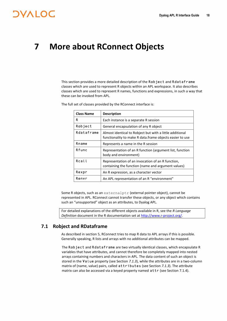
7 More about RConnect Objects

This section provides a more detailed description of the Robject and Rdataframe classes which are used to represent R objects within an APL workspace. It also describes classes which are used to represent R names, functions and expressions, in such a way that these can be invoked from APL.

The full set of classes provided by the RConnect interface is:

Class Name Description

R Each instance is a separate R session

Robject General encapsulation of any R object

Rdataframe Almost identical to Robject but with a little additional functionality to make R data.frame objects easier to use

Rname Represents a name in the R session

Rfunc Representation of an R function (argument list, function body and environment)

Rcall Representation of an invocation of an R function, containing the function (name and argument values)

Rexpr An R expression, as a character vector

Renvr An APL representation of an R “environment"

Some R objects, such as an externalptr (external pointer object), cannot be represented in APL. RConnect cannot transfer these objects, or any object which contains such an “unsupported” object as an attributes, to Dyalog APL.

For detailed explanations of the different objects available in R, see the R Language Definition document in the R documentation set at http://www.r-project.org/.

7.1 Robject and RDataframe

As described in section 5, RConnect tries to map R data to APL arrays if this is possible. Generally speaking, R lists and arrays with no additional attributes can be mapped.

The Robject and Rdataframe are two virtually identical classes, which encapsulate R variables that have attributes, and cannot therefore be completely mapped into nested arrays containing numbers and characters in APL. The data content of such an object is stored in the Value property (see Section 7.1.3), while the attributes are in a two-column matrix of (name, value) pairs, called attributes (see Section 7.1.3). The attribute matrix can also be accessed via a keyed property named attr (see Section 7.1.4).



7.1.1 Constructors

Objects are instantiated from the Robject class using one of three constructors, depending on whether zero, one or two arguments are supplied:

the first argument sets the value. The default is ⎕NULL.

the second argument sets the attributes. The default is 0 2⍴0.

For example:

⎕NEW R.object ⍝ No arguments #.[object]

⎕NEW Robject(,⊂2 2⍴⍳4) ⍝ One argument [R object: 2x2 : ]

The default display form of an instance of Robject displays the R class name (“object”), the shape of the Value property (2x2), and the list of attribute names (empty).

atts←2 2⍴'class' 'ts' 'tsp' (2014 (2014+11÷12) 12) myts←⎕NEW Robject ((?12⍴100) atts) ⍝ Two arguments

'myts' r.p myts

r.f 'myts' Jan Feb Mar Apr May Jun Jul Aug Sep Oct Nov Dec 2014 53 10 66 42 71 92 77 27 5 74 33 64

⎕←r.x 'summary(myts)' [ Min. 1st Qu. Median Mean 3rd Qu. Max. ] [ 5 31.5 58.5 51.17 71.75 92 ]

The constructors for Rdataframe are identical to those for Robject; the main advantage of the Rdataframe object is that you can create a data.frame without specifying the class name:

names←'names' ('xx' 'square') mydf←⎕NEW Rdataframe (((⍳12)∘.*1 2) names)

7.1.2 The Value property

The value of each variable within the object can be obtained or set using the Value property of any instance of the Robject or Rdataframe class:

For example:

obj←⎕NEW Robject(,⊂(2 2⍴⍳4)) obj.Value 1 2 3 4

obj.Value←4 obj.Value 4

The Value property is defined as the default property of the object, which means that it can be accessed by indexing the object using square bracket indexing or the index function ⌷. For example:


⌷obj ⍝ Returns the entire property 1 2 3 4

obj[1;] 1 2

obj[2;1]←7 ⌷obj 1 2 7 4

7.1.3 The attributes property

The attributes property returns the attributes attached to the object as a 2-column matrix of (name value) pairs. For example:

myts.attributes ⍝ with v14 ]box on ┌─────┬───────────────────┐ │tsp │2014 2014.916667 12│ ├─────┼───────────────────┤ │class│ts │ └─────┴───────────────────┘

Although all constructors accept an attribute matrix as an optional argument, attributes is read only once the object has been created. The keyed attr property must be used to change attribute values.

7.1.4 The attr property

The attr property is keyed, which means it can be used to retrieve and sets attributes, referring to them by name. For example:

obj←⎕NEW Robject ((2 2⍴⍳4) ('akey' 'itsvalue')) ⌷obj ⍝ Value is the default attribute 1 2 3 4

obj.attr[⊂'akey'] ⍝ A single name must be enclosed ┌────────┐ │itsvalue│ └────────┘

obj.attr['akey' 'dim'] ┌────────┬───┐ │itsvalue│2 2│ └────────┴───┘

dim is one of the special attributes that is widely used witin R. Where relevant, RConnect will compute these attributes on demand, validate them when set, and sometimes act upon them. For example, if dim is set, this corresponds to a “reshape” in APL:

obj.attr[⊂'dim']←4 ⍝ Change shape ⌷obj 1 2 3 4

Other “special” attributes are comment, dim, dimnames, names, row.names and tsp.


7.1.5 Changing Class

Note that the class attribute of cannot be changed directly. Instead, a new object of the required class must be instantiated from the Robject class using the appropriate constructor (see section 7.1.1).

7.2 Special Classes

In addition to Robject and Rdataframe, which cover R variables, RConnect provides a set of classes which are used to represent R expressions, functions, function calls and execution environments.

The special attributes (dim, dimnames, etc) mentioned in section 7.1.1 do not apply to the special classes. All of the objects have a constructor which allows you to set an attribute matrix, but there are currently no attributes with special meanings (however, you can always set and read attributes for your own purposes).

7.2.1 Renvr

R “environments” are similar to APL namespaces: They contain a collection of named R objects and a reference to a parent environment. Functions can be invoked within a particular environment, and many R function take an environment as a parameter. The Renvr class provides an APL representation of an R namespace, which can be modified in APL and transferred back to R. The following example creates a group of nested

environments in R, using the list2env function which converts an R list to an environment:

r.x 'P1<-list2env(list(Name="Widget",Price=42))' r.x 'P2<-list2env(list(Name="Thingy",Price=99))' r.x 'Catalog<-list2env(list(P1=P1,P2=P2))' cat←r.g 'Catalog' ⍝ retrieve it into APL

cat.Value ⍝ The Value property is a namespace #.Renvr.[Namespace] cat.Value.⎕NL -9 ⍝ Contains 2 objects P1 P2 cat.Value.P1.Value.Price 42

(⌷cat).(⌷P1).Name ⍝ Value is the default property Widget

It is also possible to manufacture an R environment from a namespace:

ns←⎕NS '' ns.(Name Value)←'Dims' 88 ⍝ A Danish widget re←⎕NEW Renvr ns 'P3' r.p ⎕NEW Renvr ns

(r.g 'P3').(Value.Name Value) Dims 88

7.2.2 Rname

The Rname class provides a container for a name in the R workspace. The Value property of an instance of Rname contains a character vector which is the name of the R variable.


An instance of Rname can be passed as a parameter to the R eval function in order to retrieve the value. For example:

'a' r.p 1 4 3 5 ⍝ Define a variable in R ⎕←an←r.g 'as.name(''a'')' ⍝ Extract it into an Rname [R name: a]

an.Value a

⎕←r.x 'eval(⍵)' an ⍝ Pass back to R to get the value 1 4 3 5

The Rname class is perhaps not particulary useful on its own, as a value can easily be retrieved using the r.g function. However, an Rname is an important component of an Rcall, which is described in the next section.

7.2.3 Rcall

The Rcall class corresponds to the call class in R, and makes it possible to represent a complete call to an R function, including arguments, as a single object. The argument values can be modified and the call can be repeated. The Value property of an instance of RCall is a vector, where the first element is an instance of Rname containing the function name, and subsequent elements are the arguments.

For example:

r.x ⍬ 'cl <- call("round", 10.5)' ⍝ Create a call r.f 'cl' round(10.5)

⎕←cl←r.g 'cl' [R call: round (1 argument)]

⎕←r.x 'eval(⍵)' cl 10

⎕←cl.Value[2]←⊂0.1×?10⍴100 ⍝ Set a different value 5.2 8.4 0.4 0.6 5.3 6.8 0.1 3.9 0.7 4.2

⎕←r.x 'eval(⍵)' cl ⍝ Repeat the call 5 8 0 1 5 7 0 4 1 4

7.2.4 Rexpr

A Rexpr is an R expression. The Value is restricted to a character string type -

representing the R code. The object can be passed to the R eval function for evaluation. For example:

⎕←r.x'eval(⍵)' (⎕NEW Rexpr(,⊂'sqrt(2+1:2-1i)')) 1.755317302J¯0.2848487846 2.015329455J¯0.2480983934

7.2.5 Rfunc

The Rfunc class makes it possible to represent an R function as an APL object. The Value property contains the body of the function, and environment a reference to the functions environment. For example:


norm←r.x 'norm'

norm.Value function (x, type = c("O", "I", "F", "M", "2")) { if (identical("2", type)) { svd(x, nu = 0L, nv = 0L)$d[1L] } else .Internal(La_dlange(x, type)) }

norm.environment getNamespace("base")

The Rfunc class makes it straightforward to define R functions from APL:

body←'function(arg1, arg2)',(⎕UCS 13),'arg1+arg2' add←⎕NEW Rfunc (,⊂body)

add.Value function(arg1, arg2) arg1+arg2 'add' r.p add ⎕←r.x 'add(3,4)' 7

The constructors for Rfunc allow you to provide an environment as the second optional argument, and an attribute as the third. If you provide an instance of an Renvr, this will be transferred together with the function when you use r.p. Alternatively, you can use the R environment method to set the environment of a function, if the environment already exists in R.

In the following example, we define a function which depends on a global variable called “basevalue”, and execute it in different environments:

body←'function(arg1)',(⎕UCS 13),'arg1+basevalue' add←⎕NEW Rfunc(,⊂body) 'add'r.p add ⍝ Transfer the function 'basevalue' r.p 42 ⍝ Give the global a value

⎕←r.x 'add(1)' 43

(E1←⎕NS'').basevalue←99 ⍝ Create a namespace 'E1' r.p ⎕NEW Renvr E1 ⍝ Save as R environment

r.x 'environment(add)<-E1' ⍝ Set environment of the fn ⎕←r.x 'add(1)' ⍝ It now picks up the global from E1 100


8 Performance Tips

Each call to the R interface has a cost; you can typically perform 20-50 calls per second, depending on your hardware and software. Data transfer rates are typically measured in megabytes per second, when transferring large arrays. If you need to make a large number of calls to R functions, each with a relatively small argument, it may be worth the effort to reduce the number of calls to R by writing an R function containing a loop, and transfer all the arguments and results in a single call.

In the following example, we show how to use this technique to generate one random number from each of thousands of beta distributions; each element of the result requiring a separate call to the “rbeta” function. We can do this by making 1000 calls via r.x as

follows:

shape1←?1000⍴10 shape2←?1000⍴10 r.x 'set.seed(123456)' 4↑dist1←{r.x (⊂'rbeta(1,⍵,⍵)'),⍵}¨shape1,¨shape2 0.4358236934 0.839276234 0.6917617888 0.412594559 On the author’s laptop, it takes roughly 25 seconds to make the 1,000 calls above. We can speed this up by almost three orders of magnitude using a loop on the R side. To do this, we create a character vector containing the body of the R function, create an instance of Rfunc containing the function, use r.p to move it to the R session, and call it:

⎕←r_fn_body ⍝ Display function definition function(alpha,beta) { for (i in 1:length(alpha)) alpha[i]<- rbeta(1,alpha[i],beta[i]) return(alpha) } 'rbetas' r.p ⎕NEW Rfunc (,⊂r_fn_body) r.x 'set.seed(123456)' 4↑dist2←r.x 'rbetas(⍵,⍵)' shape1 shape2 0.4358236934 0.839276234 0.6917617888 0.412594559 dist1≡dist2 ⍝ test that results are identical 1 On the author’s laptop, doing the loop in R takes 50-60 milliseconds, a speedup of about 500 times.


Appendix A R for APLers

This appendix provides a brief overview of some of R's functionality and the syntax necessary to achieve the required result. Where relevant, equivalent APL terminology and syntax is also provided.

The default input prompt in the R Console is >. R code in this document that does not start

with this symbol is not an input.

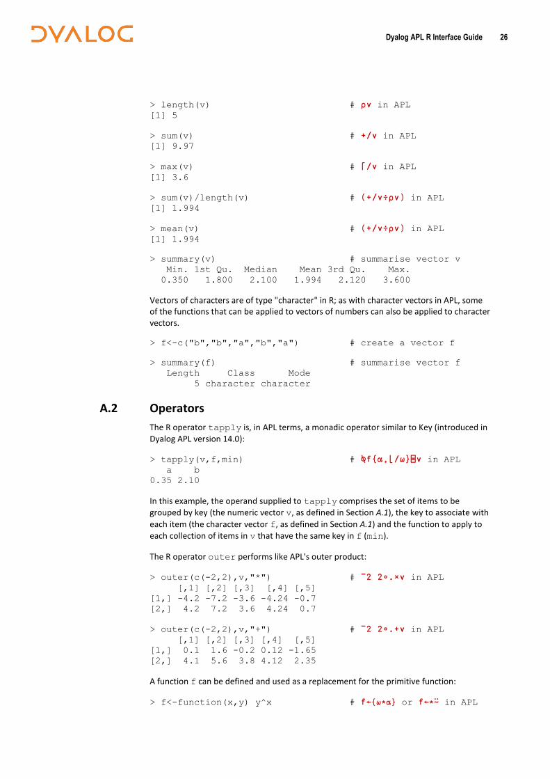
A.1 Assignment and Vector Arithmetic

R only includes a limited set of function glyphs; other mathematical operations can be performed using built-in named functions. For example, the R function to create a vector from a set of values (R does not identify individual values as scalars but rather as single-item vectors) is concatenation, written in R as c(). Scalar R functions are applied to each

element in a vector individually (pervasion in APL); scalar extension also works in R.

R's version of APL's left arrow glyph (<-) is used for assignment.

For a complete list of R's primitive functions, see the R Internals document in the R documentation set at http://www.r-project.org/.

Vectors of real (non-integer) values are of type "double" in R; as with numeric vectors in APL, these can be manipulated using a variety of mathematical functions:

> v<-c(2.1,3.6,1.8,2.12,.35) # create a vector v

> 2+v # add 2 to v

[1] 4.10 5.60 3.80 4.12 2.35

> v-1 # subtract 1 from v

[1] 1.10 2.60 0.80 1.12 -0.65

> 2*v # multiply v by 2

[1] 4.20 7.20 3.60 4.24 0.70

> v/2 # divide v by 2

[1] 1.050 1.800 0.900 1.060 0.175

> v+v # add v to v

[1] 4.20 7.20 3.60 4.24 0.70

> v^2 # square v

[1] 4.4100 12.9600 3.2400 4.4944 0.1225

where +, -, *, / and ˆ are the R symbols for addition (+), subtraction (-), multiplication (×), division (÷) and power (*) respectively.

Built-in named functions allow more complex mathematical analysis to be performed on double vectors in R:



> length(v) # ⍴v in APL [1] 5

> sum(v) # +/v in APL [1] 9.97

> max(v) # ⌈/v in APL [1] 3.6

> sum(v)/length(v) # (+/v÷⍴v) in APL [1] 1.994

> mean(v) # (+/v÷⍴v) in APL [1] 1.994

> summary(v) # summarise vector v

Min. 1st Qu. Median Mean 3rd Qu. Max.

0.350 1.800 2.100 1.994 2.120 3.600

Vectors of characters are of type "character" in R; as with character vectors in APL, some of the functions that can be applied to vectors of numbers can also be applied to character vectors.

> f<-c("b","b","a","b","a") # create a vector f

> summary(f) # summarise vector f

Length Class Mode

5 character character

A.2 Operators

The R operator tapply is, in APL terms, a monadic operator similar to Key (introduced in

Dyalog APL version 14.0):

> tapply(v,f,min) # ⍉f{⍺,⌊/⍵}⌸v in APL a b

0.35 2.10

In this example, the operand supplied to tapply comprises the set of items to be

grouped by key (the numeric vector v, as defined in Section A.1), the key to associate with

each item (the character vector f, as defined in Section A.1) and the function to apply to

each collection of items in v that have the same key in f (min).

The R operator outer performs like APL's outer product:

> outer(c(-2,2),v,"*") # ¯2 2∘.×v in APL [,1] [,2] [,3] [,4] [,5]

[1,] -4.2 -7.2 -3.6 -4.24 -0.7

[2,] 4.2 7.2 3.6 4.24 0.7

> outer(c(-2,2),v,"+") # ¯2 2∘.+v in APL [,1] [,2] [,3] [,4] [,5]

[1,] 0.1 1.6 -0.2 0.12 -1.65

[2,] 4.1 5.6 3.8 4.12 2.35

A function f can be defined and used as a replacement for the primitive function:

> f<-function(x,y) y^x # f←{⍵*⍺} or f←*⍨ in APL


> outer(c(-2,2),v,f) # ¯2 2∘.f v in APL [,1] [,2] [,3] [,4] [,5]

[1,] 0.2267574 0.07716049 0.308642 0.2224991 8.163265

[2,] 4.4100000 12.96000000 3.240000 4.4944000 0.122500

A.3 Arrays

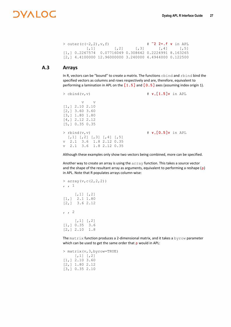
In R, vectors can be “bound” to create a matrix. The functions cbind and rbind bind the specified vectors as columns and rows respectively and are, therefore, equivalent to performing a lamination in APL on the [1.5] and [0.5] axes (assuming index origin 1).

> cbind(v,v) # v,[1.5]v in APL

v v

[1,] 2.10 2.10

[2,] 3.60 3.60

[3,] 1.80 1.80

[4,] 2.12 2.12

[5,] 0.35 0.35

> rbind(v,v) # v,[0.5]v in APL [,1] [,2] [,3] [,4] [,5]

v 2.1 3.6 1.8 2.12 0.35

v 2.1 3.6 1.8 2.12 0.35

Although these examples only show two vectors being combined, more can be specified.

Another way to create an array is using the array function. This takes a source vector and the shape of the resultant array as arguments, equivalent to performing a reshape (⍴) in APL. Note that R populates arrays column-wise:

> array(v,c(2,2,2))

, , 1

[,1] [,2]

[1,] 2.1 1.80

[2,] 3.6 2.12

, , 2

[,1] [,2]

[1,] 0.35 3.6

[2,] 2.10 1.8

The matrix function produces a 2-dimensional matrix, and it takes a byrow parameter

which can be used to get the same order that ⍴ would in APL:

> matrix(v,3,byrow=TRUE)

[,1] [,2]

[1,] 2.10 3.60

[2,] 1.80 2.12

[3,] 0.35 2.10


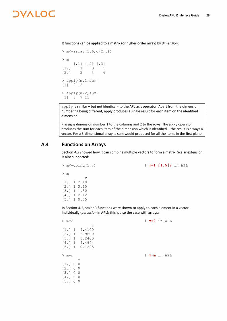
R functions can be applied to a matrix (or higher-order array) by dimension:

> m<-array(1:6,c(2,3))

> m

[,1] [,2] [,3]

[1,] 1 3 5

[2,] 2 4 6

> apply(m,1,sum)

[1] 9 12

> apply(m,2,sum)

[1] 3 7 11

apply is similar – but not identical - to the APL axis operator. Apart from the dimension numbering being different, apply produces a single result for each item on the identified dimension.

R assigns dimension number 1 to the columns and 2 to the rows. The apply operator produces the sum for each item of the dimension which is identified – the result is always a vector. For a 3-dimensional array, a sum would produced for all the items in the first plane.

A.4 Functions on Arrays

Section A.3 showed how R can combine multiple vectors to form a matrix. Scalar extension is also supported:

> m<-cbind(1,v) # m←1,[1.5]v in APL

> m

v

[1,] 1 2.10

[2,] 1 3.60

[3,] 1 1.80

[4,] 1 2.12

[5,] 1 0.35

In Section A.1, scalar R functions were shown to apply to each element in a vector individually (pervasion in APL); this is also the case with arrays:

> m^2 # m*2 in APL v

[1,] 1 4.4100

[2,] 1 12.9600

[3,] 1 3.2400

[4,] 1 4.4944

[5,] 1 0.1225

> m-m # m-m in APL v

[1,] 0 0

[2,] 0 0

[3,] 0 0

[4,] 0 0

[5,] 0 0


Like APL, R functions can take arguments that are of different rank, for example, a vector and a matrix as long as they are of compatible proportions:

> v*m # v×[1]m in APL v

[1,] 2.10 4.4100

[2,] 3.60 12.9600

[3,] 1.80 3.2400

[4,] 2.12 4.4944

[5,] 0.35 0.1225

For matrix multiplication, R uses %*%:

> v%*%m # v+.×m in APL v

[1,] 9.97 25.2269

> t(m)%*%m # (⍉m)+.×m in APL v

5.00 9.9700

v 9.97 25.2269

where the R function t()transposes the specified matrix.

A.5 Data Frames

A data frame in R can be thought of in APL terms as a nested matrix with named columns and rows (from some perspectives, a data frame can also be thought of as an APL namespace containing multiple vectors of the same shape). The columns of the data frame can each be of a different type if required. A data frame often has a names attribute and a

row.names attribute specifying the names to use for the columns and rows of the data frame respectively.

A data frame can be created using a number of vectors and the R function data.frame.

First, the vectors need to be defined:

> x<-rnorm(5)

> y<-rnorm(5)

> z<-rnorm(5)

> f<-c("one", "two", "one", "two", "two")

These vectors can then be used to define the data frame:

> df<-data.frame(alpha=x,

+ beta=y,

+ gamma=z,

+ class=f)

If a definition is started directly in R rather than in an editor, then the + sign is automatically placed at the start of each line following an opening parenthesis to indicate that the definition is not complete. This continues until a closing parenthesis is used and the command is syntactically complete.

R's print function can be used to display the data frame in the R Console with row and

column headings:


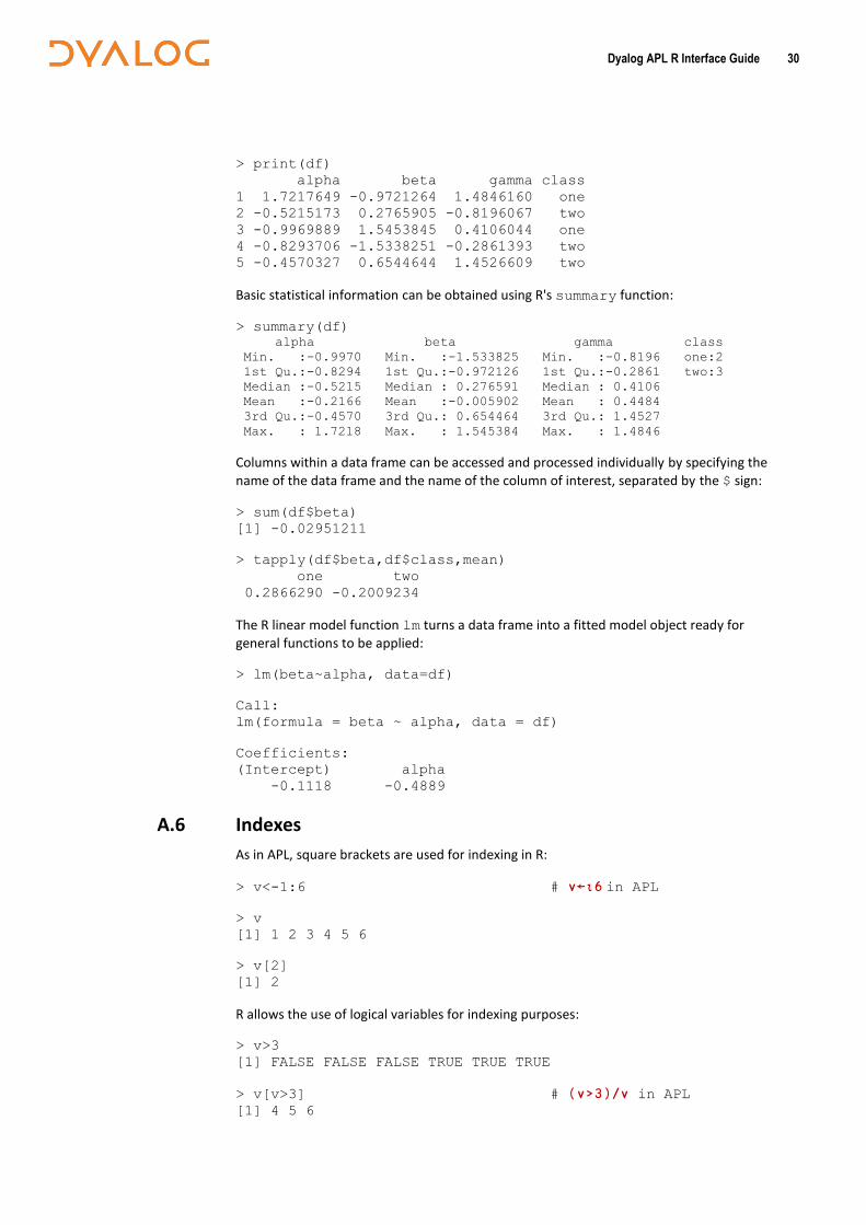
> print(df)

alpha beta gamma class

1 1.7217649 -0.9721264 1.4846160 one

2 -0.5215173 0.2765905 -0.8196067 two

3 -0.9969889 1.5453845 0.4106044 one

4 -0.8293706 -1.5338251 -0.2861393 two

5 -0.4570327 0.6544644 1.4526609 two

Basic statistical information can be obtained using R's summary function:

> summary(df)

alpha beta gamma class

Min. :-0.9970 Min. :-1.533825 Min. :-0.8196 one:2

1st Qu.:-0.8294 1st Qu.:-0.972126 1st Qu.:-0.2861 two:3

Median :-0.5215 Median : 0.276591 Median : 0.4106

Mean :-0.2166 Mean :-0.005902 Mean : 0.4484

3rd Qu.:-0.4570 3rd Qu.: 0.654464 3rd Qu.: 1.4527

Max. : 1.7218 Max. : 1.545384 Max. : 1.4846

Columns within a data frame can be accessed and processed individually by specifying the

name of the data frame and the name of the column of interest, separated by the $ sign:

> sum(df$beta)

[1] -0.02951211

> tapply(df$beta,df$class,mean)

one two

0.2866290 -0.2009234

The R linear model function lm turns a data frame into a fitted model object ready for

general functions to be applied:

> lm(beta~alpha, data=df)

Call:

lm(formula = beta ~ alpha, data = df)

Coefficients:

(Intercept) alpha

-0.1118 -0.4889

A.6 Indexes

As in APL, square brackets are used for indexing in R:

> v<-1:6 # v←⍳6 in APL

> v

[1] 1 2 3 4 5 6

> v[2]

[1] 2

R allows the use of logical variables for indexing purposes:

> v>3

[1] FALSE FALSE FALSE TRUE TRUE TRUE

> v[v>3] # (v>3)/v in APL [1] 4 5 6


For matrices and higher order arrays R uses the , character to separate the dimensions – APL uses the ; character:

> m<-array(v,c(2,3))

> m

[,1] [,2] [,3]

[1,] 1 3 5

[2,] 2 4 6

> m[1,2]

[1] 3

As in APL, R allows the selection of a single row and column from a matrix:

> m[1,]

[1] 1 3 5

> m[,3]

[1] 5 6

An index can be specified using a vector:

> v[c(3,3,4,1)] # v[3 3 4 1] in APL [1] 3 3 4 1

If an index is a matrix, then a vector of values is returned:

> v[array(c(3,3,4,1),c(2,2))] # v[,2 2⍴3 3 4 1] in APL [1] 3 3 4 1

An array can also be used for indexing purposes:

> i<-array(c(1,1,2,3,1,3),dim=c(3,2))

> i

[,1] [,2]

[1,] 1 3

[2,] 1 1

[3,] 2 3

> m[i] # m[↓i] in APL [1] 5 1 6

This can be extended by using the index to assign replacement values:

> m[i]<-0 # m[↓i]←0 in APL

> m

[,1] [,2] [,3]

[1,] 0 3 0

[2,] 2 4 0

A logical array can also be used to index a matrix (similar to applying a Boolean mask in APL):

> m==0 # m=0 in APL [,1] [,2] [,3]


[1,] TRUE FALSE TRUE

[2,] FALSE FALSE TRUE

> m[m==0]<-99

> m

[,1] [,2] [,3]

[1,] 99 3 99

[2,] 2 4 99

A.7 Defined Functions

New functions are defined using the following R expression:

function_name<-function(args) expr

where:

function_name is the name of the new function

args is one or more arguments separated by the , character

expr is the expression that defines the function

Simple functions can be defined on a single line (more complicated functions might require multiple line definitions):

> foo<-function(x) x*3 # foo←{⍵×3} in APL

> foo(4)

[1] 12

> foo(5)

[1] 15

In R, default values can be set for some arguments. This is illustrated by the following example, which calculates a probability density function for normal (Gaussian) distribution. The equation for this is:

f(x, μ, σ) =1

√2𝜋𝜎𝑒−(𝑥−𝜇)2

2𝜎2

In R this equation is implemented as:

> gauss<-function(x,mu=0,sd=1){

+ fx<-exp(-((x-mu)^2)/(2*sd^2))

+ fx/(sqrt(2*pi)*sd)

+}

Setting default values for and means that the function can be called with only x specified:

> gauss(0)

[1] 0.3989423

> gauss(1.5)

[1] 0.1295176

The default value for an argument can be overridden either by specifying the value to use for that argument using its position in the list of arguments:


> gauss(0,0,3)

[1] 0.1329808

or by specifying the name of the argument that the value is for:

> gauss(0,sd=3)

[1] 0.1329808


Appendix B References for R

The following links provide comprehensive information on the history, capabilities and syntax of R:

The R Project for Statistical Computing: http://www.r-project.org/

The Comprehensive R Archive Network: http://cran.r-project.org/

R Wiki: http://rwiki.sciviews.org/doku.php

Google's R Style Guide: http://google-styleguide.googlecode.com/svn/trunk/google-r-style.html



http://rwiki.sciviews.org/doku.php

http://google-styleguide.googlecode.com/svn/trunk/google-r-style.html

Dyalog APL R Interface Guide

Documents

Transcript of Dyalog APL R Interface Guide