)DWLJXH DQG dynamics of secondary beams in steel railway ...743366/FULLTEXT01.pdf · Fatigue and...
82
0$67(5 2) 6&,(1&( 7+(6,6 672&.+2/0 6:('(1 )DWLJXH DQG dynamics of secondary beams in steel railway bridges 3((7(5 .$17(5 KTH ROYAL INSTITUTE OF TECHNOLOGY SCHOOL OF ARCHITECTURE AND THE BUILT ENVIRONMENT
Transcript of )DWLJXH DQG dynamics of secondary beams in steel railway ...743366/FULLTEXT01.pdf · Fatigue and...

dynamics ofsecondary beams in steelrailway bridges
KTH ROYAL INSTITUTE OF TECHNOLOGY
SCHOOL OF ARCHITECTURE AND THE BUILT ENVIRONMENT


Fatigue and dynamics ofsecondary beams in steelrailway bridges
Peeter Kanter
May 2014 TRITA-BKN. Master Thesis 408, 2014 ISSN 1103-4297 ISRN KTH/BKN/EX-408-SE

©Peeter Kanter, 2014 Royal Institute of Technology (KTH) Department of Civil and Architectural Engineering Division of Structural Design and Bridges Stockholm, Sweden, 2014

i
Preface
First of all I would like to thank my supervisor John Leander for giving guidance during this project. I have learned a lot! I am also grateful towards professor Raid Karoumi for letting me work on this interesting topic at the Department of Civil and Architectural Engineering, Division of Structural Engineering and Bridges.
I would also like to thank all my fellow students who supported me during this thesis. I would especially like to thank Angela and David for proof-reading my thesis.
Stockholm, May 2014
Peeter Kanter


iii
Abstract
Many steel railway bridges in Europe are older than 50 years while they are subjected to higher loads than they were originally designed for. As many of these bridges are approaching the end of their design life it is crucial to carry out accurate fatigue assessments in order to ensure their safety and keep them in service. Usually the influence of dynamics on fatigue damage is taken into account using dynamic amplification factors from design codes whereas the actual influence of dynamics has not been thoroughly studied.
During this study the importance of dynamics on fatigue damage is examined on two specific examples, namely the Söderstöm Bridge and the Åby älv bridge, which are good examples of open deck bridges that are common among steel railway bridge population.
Different train speeds, the cross beam effect and load distribution were studied in order to assess the importance of dynamics on fatigue damage. Three dimensional finite element models were created and later modified to perform dynamic analysis. Moving point loads were used to simulate the loading of moving trains. Fatigue damages were calculated at the various locations to evaluate the influence of dynamics on fatigue damage.
The results show that the dynamics has small influence on fatigue damage at studied speeds and damage is not dependent on speed. Assessed cross beam effect was not detected on studied bridges in terms of dynamics, but has great influence in terms of statics.


v
Contents
Preface ................................................................................................. i
Abstract ............................................................................................. iii
Contents .............................................................................................. v
1 Introduction ............................................................................. 1
1.1 Background ...................................................................... 1
1.2 Aim and scope .................................................................. 3
2 Case Studies ............................................................................. 5
2.1 The Söderström Bridge .................................................... 5
2.1.1 Location and importance ..................................... 5
2.1.2 Geometry and structural system .......................... 7
2.1.3 Loading .............................................................. 10
2.1.4 Inspections ......................................................... 11
2.1.5 Monitoring program and previous studies ........ 13
2.2 The Åby älv bridge ......................................................... 15
2.2.1 General information .......................................... 15
2.2.2 Geometry and structural system ........................ 15
2.2.3 Loading .............................................................. 17
3 Cross beam effect .................................................................... 19

vi
4 Finite Element Modelling ....................................................... 23
4.1 Finite element models ................................................... 23
4.2 Solution methods ............................................................ 28
4.3 Damping ......................................................................... 29
4.4 Loading ........................................................................... 30
4.5 Comparison with measured results ................................. 33
4.5.1 The Söderström Bridge ..................................... 33
4.5.2 The Åby älv bridge ............................................ 35
5 Fatigue assessment .................................................................. 37
5.1 Fatigue ........................................................................... 37
5.2 Stress concentrations ...................................................... 39
5.3 Fatigue evaluation according to Eurocode ..................... 41
5.3.1 S-N design curves .............................................. 41
5.3.2 Cycle counting methods .................................... 43
5.3.3 Fatigue life prediction ....................................... 45
5.4 Fatigue assessment for the models ................................. 48
6 Results ...................................................................................... 53
6.1 Influence of different train speeds .................................. 53
6.2 Influence of load distribution ......................................... 56
6.3 Influence of the cross beam effect .................................. 58
7 Discussion and conclusions .................................................... 65
7.1 Discussion ...................................................................... 65
7.2 Conclusions .................................................................... 67
Bibliography .................................................................................... 69

Introduction
1
1 Introduction
1.1 Background
A substantial population of the steel railway bridges in Europe are older than 50 years. A survey was carried out [Bell, 2004] where more than 40,000 steel railway bridges were studied and it was shown that 60% of these bridges were older than 50 years. Many of these bridges (28%) have already exceeded their design work life (100 years). To make matters worse these bridges are often exposed to higher axle loads and larger traffic volume than they were originally designed for. In order to keep these bridges in service and ensure their safety, various repair works or strengthening methods might be necessary. For most of these bridges an ‘open deck solution’ was used during the building process; especially steel railway bridges built in the 1950s and 1960s are of this type [Huanga, 2001]. However, there are an insufficient amount of monetary funds available to replace them just because they have exceeded their design work life. Even if funds would be readily available, replacement of many of these bridges would be difficult because of their historic importance or their strategic location in the railway network [Sedlacek, 2008].
There are a number of causes that can lead to the failure of open deck bridges. In a survey [Oehme, 1989] these types of causes for different steel structures were analysed. 16.1% of the damaged structures
Chapter

Introduction
2
analysed in this survey were railway bridges. This ranks steel railway bridges as the second most damaged structures analysed [Sedlacek, 2008]. In table 1.1 the main causes for the failure of steel structures are listed. The table shows that fatigue is the most frequently encountered reason for failure. Fatigue can therefore be considered as the factor that limits the service life of steel railway bridges.
Table 1.1: Main causes that lead to damage of steel structures [Sedlacek, 2008].
Since fatigue is the main reason for structural failure in the case of open deck railway bridges, methods investigating fatigue damage are important. On many occasions [Stamatopoulos, 2012. Zabel, 2013. Caglayan, 2008] this is done using comprehensive methods, including advanced material testing and field measurements.
On many occasions, initial assessments are conducted through theoretical studies using the guidelines given in the design codes. Often when these type of studies [Brühwiler, 2013. Gambarotta, 2008] are carried out the influence of the dynamic behaviour of the bridge is taken into account by using a dynamic amplification factor When conventional fatigue assessments are performed the dynamic amplification factor is given by equation (1) where is associated with the dynamic behaviour of the bridge and is associated with the track irregularities [EN-1991-2].

Introduction
3
1 (1)
This provides us with a linear amplification of the stress amplitudes. Distribution of the cycles between stress ranges and the number of cycles is not affected.
However, the actual impact of the dynamic loads on fatigue damage in general has not been thoroughly studied. The influence of the dynamic loading was recently studied more extensively in [Leander, 2013]. The analytical model that was used in this study was limited to two dimensional beams with simple support conditions.
The Söderström Bridge and the Åby älv bridge (see Chapter 2) are good examples of open deck bridges for studying the effect of the dynamic loading on fatigue damage. Both of the bridges have an open deck structure that is built using short thick beam elements. These beam elements have bracing systems that impose fatigue critical connections. Both bridges are therefore suitable for studying the influence of dynamic loading on fatigue damage.
1.2 Aim and scope
The main goal of this thesis is to investigate the influence of dynamic loading on fatigue damage by using the examples of the Söderström Bridge and the Åby älv bridge. The bridges are studied using the Finite Element Method (FEM) which enables one to consider more complex structural behaviour. The emphasis of this research is on investigating secondary structural elements such as cross beams and stringer beams. The different aspects that influence fatigue damage are studied. The influence of the train speed on dynamic loading and fatigue damage is studied and compared with the results obtained using the guidelines given in the Eurocode. The influence of the load distribution proposed in the Eurocode for assessment of fatigue damage is investigated. Different aspects of the interaction between secondary structural elements and the cross beam effect are studied by evaluating changes in fatigue damage.

Introduction
4
The goals are reached by using the following methodology. First the models of the bridges are created using the Finite Element (FE) software ABAQUS. Secondly the general behaviour of the models is checked by comparing the results of the model with existing field measurements. Finally different analyses are performed using different train types and train speeds.
In order to achieve the goals of this study, the following assumptions have been made, and limitations observed:
The bridges are modelled using a 3D FE model. Only beam and truss elements are used during the study.
The study is limited by using only three different train load models.
The suspension system of the train is not modelled in load modelling. Moving concentrated point loads are used.
Track irregularities are not taken into account during the modelling.
Sleepers, rails and other non-structural elements are not modelled. Their mass is included in the mass of the structural elements.

Case Studies
5
2
Case Studies
2.1 The Söderström Bridge
2.1.1 Location and importance
The Söderström Bridge, built in the beginning of 1950’s, is situated in the central part of Stockholm where it carries a vital role for one of the most important railway lines in Sweden. The bridge is part of the line that connects the northern and southern parts of Sweden, specifically the Central Station and the South Station of Stockholm. It crosses Riddarfjärden (bay of Lake Mälaren) and connects Södermalm Island with Riddarholmen Island. The location of the bridge is marked with red in figure 2.1.
Chapter

Case Studies
6
Figure 2.1: A map of the area between Central Station and South Station.
In figure 2.2 the railway network of Stockholm area is displayed. The figure shows that all the railway lines come together at a bottleneck located in the central part of Stockholm. The Söderström Bridge is part of that bottleneck. There are 10 pairs of tracks at the Central Station side and 4 pairs of tracks at the South Station side that narrow down into 2 pairs of tracks between two stations. The bridge carries three different types of train traffic: regional commuter trains (Pendeltåg), national commuter trains and freight trains.
Every day about a quarter of a million passengers use local commuter trains [Rönnberg, 2010]. The larger cities of Sweden, besides Stockholm, lie south of Stockholm and since Stockholm is used as a start/end station by about 80% of the national commuter trains in Sweden, [Rönnberg, 2010] the Söderström Bridge plays a crucial role in the whole transportation system of Sweden. The current line, consisting of two tracks, is occupied by traffic 81-100 % of the time during rush hours. As a consequence of the limited capacity of the bridge, local commuter trains are often overcrowded and delays are common. [Rönnberg, 2010]. About 520 trains pass the line every day [Leander, 2010].

Case Studies
7
Figure 2.2: Overview of the Swedish railway network in the Stockholm region.
The situation is going to stay critical until 2017 when the construction of the Citybanan will be completed. The tunnel will add 2 new tracks and with that will double the capacity of the overcrowded bottleneck. All the regional commuter trains will be supported by the tunnel, which will improve the situation of the current line considerably as the regional commuter trains use up to 60% of current total capacity [Leander, 2010]. The introduction of the tunnel will make reconstruction or repair works on the Söderström Bridge considerably easier.
2.1.2 Geometry and structural system
The Söderström Bridge is a skewed six span continuous steel beam bridge with a total length of 188.6m. The spans have lengths of 27.0, 33.7, 33.7, 33.7, 33.6 and 26.9 meters respectively. The northern part of the bridge is straight; the southern part is curved with a constant radius of 2500 meters. The three northern spans are straight (between supports 4 and 7) and the curve is formed between supports 7 and 10 (see figure 2.3). The substructure of the bridge is resting on piled concrete slab foundations. Piles have been driven until the solid

Case Studies
8
bedrock. The northern support is formed by an abutment consisting of breast and wing walls.
Figure 2.3: A plan and a side view of the bridge.
Intermediate supports are formed by circular piers. The southern abutment is a rectangular column. Fixed bearings are used at support 10, while all the other supports have roller bearings, which allow movement in the longitudinal direction. Rotation around a horizontal axis perpendicular to the longitudinal direction of the bridge is not restricted by any bearings.
The superstructure is a continuous grillage forming an open deck configuration. The deck has to carry two pairs of tracks. The tracks are resting on wooden sleepers that are bolted onto I-profile stringer beams. Stringer beams are welded to the I-profile cross beams throughout the whole structure. The span of the stringer beams between cross beams varies from 3.360 to 3.375 meters. The cross beams have a skew angle of 79.7°, measured in relation to the stringer and the main beams orientations. The cross beams have a span of 10.2 meter and they are welded to two main I-profile girders.

Case Studies
9
Figure 2.4: Detailed plan of the span between supports 6 and 7
In addition to the main load bearing system there are multiple bracing systems. Their function is to prevent lateral movement of the bridge and to reduce torsion in some of the beams that they are connected to. The wind bracing system is formed by connecting the cross beams midpoint to the main beams. Connections are made between the bottom flanges. The zigzag bracing system is positioned between the stringer beams which restrain torsion and movement of the stringer beams. The system is formed by connecting the midpoints of the stinger beam with a neighbouring stringer beam from three different points (the end points and the middle). All the connections between stringer beams are made between the upper flanges of the beams. In order to transfer acceleration or braking forces created by trains from the stringer beams down to main load carrying system and further onto substructure an additional bracing system is used. The system is located adjacent to the supports. In order to form a bracing connection between the different types of beams steel plates are welded to these beams. Bracing elements (L- or T-profile) are connected to the steel attachment plates either by bolted or riveted connections. The location and exact positioning of the bracing systems is shown in the figure 2.4.

Case Studies
10
Figure 2.5: Cross-section through the superstructure
2.1.3 Loading
The Söderström Bridge was designed using contemporary design codes, specifically for the train load type F46, shown in figure 2.6. Nowadays this bridge is classified using train load type D2, shown in figure 2.6. An arbitrary number of waggons should be considered when using the load type D2 in order to accomplish critical loading. Currently the most prevalent type of trains on the bridge is passenger trains. According to studies, only 7% of the total passes are made by freight trains. 60% of the total passes on the bridge are made by commuter trains, mainly by the Swedish X60 type of train (see figure 3). The X60 trains have a maximum axel load of 210 kN.
In addition to the structural elements (main beams, cross beams, stringer beams and different bracing systems) the bridge must carry the load of the non-structural elements. The main beam on the western side of the bridge is carrying a pedestrian walkway. The main load is applied to the bridge by the walkway’s 80mm thick concrete deck. The stringer beams carry the load of the sleepers and the rails. The cross beams need to carry the additional weight of 3 cable ducts; the concrete duct in the middle of the tracks and the steel ducts between the main beams and the adjacent stringer beams. The non-structural elements are illustrated in grey in figure 2.5.

Case Studies
11
Figure 2.6: Train load types for bridge design and assessment
Figure 2.7: Swedish commuter train X60
2.1.4 Inspections
Cracks in the welds between the stiffener and the webs of the main beams were discovered while regular inspections were performed on the Söderström Bridge. A location of a crack is shown in figure 2.8. After these discoveries extensive inspections were carried out.

Case Studies
12
According to a technical report [Ekelund, 2008] 90 cracks were discovered in the main beam webs. Out-of-plane bending of the web of the main beams is believed to be a reason for the formation of the cracks. The crack propagation in the weld between the stiffener and the web of the main beam can be defined as ‘displacement controlled.’ Further propagation of the crack would result in a change of the static system of the cross beam. The cross beam would function as a simply supported beam [Leander, 2010].
Figure 2.8: A location of a crack in the weld between the main beam web and the stiffener.
The results of the inspections [Pettersson, 2010] held in 2010 were more alarming. Cracks in the welds between the bottom flanges of the cross beams and the attachment plates of the wind bracing system were found. A location of a crack is shown in figure 2.9. The crack’s propagation in the connection can be defined as load controlled which can be considered extremely dangerous, as there are no other possible alternative load paths [Leander, 2010].
Figure 2.9: A location of a crack in the weld between the cross beam and the attachment plate.

Case Studies
13
2.1.5 Monitoring program and previous studies
Interest in the Söderström Bridge rose considerably after the cracks in the web of the main beams were discovered. The cracks in the main beam webs indicated a need for a theoretical study because potentially far more critical connections could be found. A large amount of bracing system connections involving poorly designed welded attachment plates was found. A typical type of connection is illustrated in figure 2.9. More than 800 connections were found to be critical.
In a study [Andersson, 2009] a theoretical fatigue assessment was conducted by using the following guidelines: Swedish Regulations for Steel Structures and the Swedish Regulations for the capacity assessment of existing railway bridges. A 3D finite element (FE) model using 3D Euler-Bernoulli beam elements was created in order to calculate nominal stress ranges in the critical sections. Three different methods were used during the fatigue evaluation process. Method 1, which is mostly used during the design stage or during the evaluation of the existing bridges, indicated that there is a risk of fatigue damage in all of studied elements. The use of the more accurate methods 2 and 3, which consider the real loading conditions on the bridge, confirmed the initial suspicions. The estimated fatigue life for the main beams would be 70 years, for the cross beams 30 years and only a few years for the stringer beams if the continuation of the current loading conditions is assumed.
As a result of the alarming discoveries that were found during the theoretical fatigue assessment an extensive monitoring program was developed. Thorough non-destructive methods and field measurements were used during the monitoring program. The use of the non-destructive methods, however, did not confirm the critical results related to the stringer beams. No indication of the fatigue-related damage was found. In order to take measurements the stringer beams, the cross beams and the main beams were fitted with strain gauges and accelerometers. The measurements were taken

Case Studies
14
continuously over a period of 43 days. The continuous measurements made it possible to take into account the real variations of traffic, which increased the accuracy of the estimated yearly traffic volume and loading condition. A far more accurate fatigue assessment was carried out thanks to extensive high quality data. The alarming results for the stringer beams were confirmed as a more favourable stress range spectra was not found. In addition, more sections with a high risk of fatigue-related damage were discovered. The attachment plates of the wind bracing systems, which are welded to the cross beams, had created potentially hazardous sections. Due to the discovered peak stresses the accumulated damage is alarmingly high in the cross beam section. The results of the fatigue assessment for that cross section were later confirmed by the cracks that were found during the inspections held in 2010.
The large amount of high quality data collected during the monitoring program provided a good basis for more accurate finite element models that could be used for further studies. This information was used during the study [Wallin, 2011] which was held to investigate the possibilities to strengthen the bridge. Two different strengthening systems were under consideration. The modification of the structural system by adding additional arches under the superstructure was considered as one of the solutions. The other method involved tensioning of the cross beams. Both methods were investigated using 3D finite element models verified with field measurements. Different types of dynamic analysis were performed using moving train loads. Both methods proved to be suitable and showed positive effects on the bridge’s fatigue life.
Gathered data was also used in the study [Kaliyaperumal, 2010] dealing with modelling techniques regarding dynamic analysis. Different types of models with varying levels of complexity were created and then the results of the analysis were compared to the measured results. The study contained an eigenvalue analysis and a time history dynamic analysis using different trains and train speeds.
.

Case Studies
15
2.2 The Åby älv bridge
2.2.1 General information
The Åby älv bridge (shown in Figure 2.10) was built in 1957 to cross river Åby in the north of Sweden where it was a part of the Malmbanan railway line. The bridge is currently not in service. The bridge was replaced during a bridge replacement programme in October 2012. The bridge was placed on temporary supports near its original location for some further testing.
Figure 2.20: A picture of the Åby älv bridge [Andersson, 2013].
2.2.2 Geometry and structural system
The Åby älv bridge is a simply supported bridge with a span of 33 meters. The deck is carrying one pair of tracks. The tracks are resting on wooden sleepers that are bolted onto I-profile stringer beams.

Case Studies
16
Figure 2.11: A side and a plan view of the Åby älv bridge.
The superstructure is formed by using two Warren trusses with verticals. The lower cords of the trusses are made from U-profile sections. The upper cords of the trusses are formed using hollow rectangular box sections. The verticals and diagonals are built using I-profile beams. The truss members are connected to each other using bolted connections. The lower cords of the trusses are connected with crossbeams. The cross beams have span of 5.5 meters. They are formed using I-profile beam sections that have variable height cross-section near the trusses in order to form a more rigid connection. Stringer beams are placed between the crossbeams in order to carry traffic loads. The span of the I-profile stringer beams is 4.125 meters. The stringer beams are connected to the crossbeams using riveted connections.
The bridge has multiple bracing systems. The Åby älv bridge has a similar zigzag bracing system as the Söderstöm Bridge which is positioned between the stringer beams and restrains torsion and movement of the stringer beams. The lower cords of trusses are connected using wind bracings. The upper cords of the trusses, however are not braced which is uncharacteristic of these type of bridges. Bracing elements (L- or T-profile) are connected to the steel

Case Studies
17
attachment plates either by bolted or riveted connections. The location and exact positioning of the bracing systems is shown in the figure 2.11.
Figure 2.12: Cross-section through the superstructure
2.2.3 Loading
The Åby älv bridge was designed using contemporary design codes, similar to that of the Söderstöm Bridge, for the train load type F46 as shown in figure 2.6.

Case Studies
18
In addition to the structural system the bridge is carrying the load of the non-structural elements. The stringer beams carry the load of the sleepers and the rails. The cross beams are also supporting lightweight steel footpaths. The non-structural elements are illustrated in grey in figure 2.12.

Cross beam effect
19
3
Cross beam effect
The cross beam effect of steel railway bridges comprises the dynamic effects of the trains passing along an open deck bridge. This effect is found in classical type open deck bridges that have longitudinal stringer beams and transversal cross beams. A typical layout of this type of deck grillage is illustrated in figure 3.1.
The cross beam effect appeared after the introduction of new types of locomotives such as electric and diesel-electric. These types of locomotives have boogies and spacing between their wheels which often increases the cross beam effect [Fryba, 1996].
Chapter

Cross beam effect
20
Figure 3.1: Deflections of an open deck grillage [Fryba, 1996].
The stiffness of this type of bridge deck varies along its length. The stiffness of the bridge deck is highest at the cross beams and lowest at the mid-span of the stringer beams. A passing train produces varying deflections along the deck (see figure 3.1). The deflections are largest at the mid-spans of the stringer beams and smallest above the cross beams. Varying deflections create an undulated curved pathway when the train moves along the deck. These irregularities arise from the mutual interaction between the bridge and the train as an integral dynamic system. The cross beam effect of a deck with varying stiffness can be described by a system of closely spaced elastic springs of variable stiffness along the bridge length as shown in figure 3.2.
Figure 3.2: Representation of a bridge deck as an elastic layer of variable stiffness [Fryba, 1996].

Cross beam effect
21
The cross beam effect is examined in [Leander, 2013]. The influence of support stiffness (for example a cross beam’s stiffness) on the continuous beam’s fundamental frequency is studied. The fundamental frequencies of continuous beams are lowered when support stiffness is lowered which can causes resonance for some loading conditions. The results in [Leander, 2013] also imply that support stiffness can have influence on structures dynamic behavior.

Cross beam effect
22

Finite Element Modelling
23
4
Finite Element Modelling
4.1 Finite element models
In order to assess the fatigue damage of the open deck bridges under moving dynamic loading finite element models of the Söderström Bridge and the Åby älv bridge were created using the commercial FE-analysis software ABAQUS. The 3D beam models (see figure 4.1 and 4.2) were created according to the original drawings. As the focus of this research was set on studying the fatigue damage of the stringer beams and the cross beams only two spans of the Söderstöm Bridge were modelled (the spans between support 5 and 7). The Åby älv bridge consists of only one span and was therefore modelled completely.
Chapter

Finite Element Modelling
24
Figure 4.1: Visualization of the 3D finite element model of the Söderström Bridge
The models were created by using beam and truss elements. The main structural members such as the main beams, the truss cords, the cross beams and the stringer beams were modelled using Timoshenko beam elements. These types of elements were chosen because of their ability to consider shear deformations and rotation inertia, which is important when short thick beams are studied. The decks were modelled as a grillage. All the beam elements were connected using rigid links. Eccentricities were given to the beam elements in order to determine their exact location in the model. All the bracing systems were modelled using truss elements in order to avoid their local behaviour from influencing the results. The beam and the truss elements were connected using the kinetic coupling constraints that are available in ABAQUS.
The initial models were created using the original section properties of the bridge. As all structural elements of the bridge are made out of steel, the following material properties were used: Young’s modulus E = 210 GPa, Poisson’s ration ν = 0.3 and density ρ = 7800 kg/m3. As

Finite Element Modelling
25
the sleepers and the rails were not modelled, the moving train loads were applied directly onto the stringer beams.
Figure 4.2: Visualization of the 3D finite element model of the Åby älv bridge.
The influence of the non-structural elements was included by increasing the density of the structural members that are subjected to the loading of the non-structural elements. In the case of the Söderström Bridge the load of the pathway was added to the western main girder. The weight of the cable ducts were added to the cross beam section that are directly subjected to the loading of the cable ducts. The loading of the sleepers and the rails were added to the stringer beams. The largest change in density was required for the stringer beams, which had the fictitious density of 13300 kg/m3. In the case of the Åby älv bridge only the loading of the sleepers and the

Finite Element Modelling
26
rails were added to the stringer beams. That resulted in the fictitious material density of 13200 kg/m3 for the stringer beams.
Figure 4.3: The Söderström Bridge model’s first span (between supports 5 and 6), support conditions. (1) Pinned support. (2) Roller support.
To create a support equivalent to the support conditions of the real bridge the following boundary conditions were applied to the Söderström Bridge model. Pinned supports were created by restraining all the displacements and were used at the first support (support 5) (see figure 4.3). Roller supports were used for the other supports. They restrain displacements in the vertical and the transversal direction and allow movement in the longitudinal direction (see figure 4.3). Similar boundary conditions were applied while modelling the Åby älv bridge as the bridge is simply supported. Pinned supports were used on one end of the bridge model’s corners and roller supports were used at the other end’s corners.
The influence that the cross beam effect and interaction of secondary structural elements have on the fatigue damage was studied through different modifications. The effect on fatigue damage was studied through varying the stiffness of the existing system and modifying the structural system. In the case of the Söderström Bridge the original model material properties were modified in order to investigate the

Finite Element Modelling
27
change in fatigue damage when the system’s stiffness was increased. Values of the Young’s modulus were modified in order to change the stiffness of the structural system. The model was modified according to the three following ways:
1. First only the Young’s modulus of the main beams was modified.
2. Then only the Young’s modulus of the cross beams was modified.
3. Finally both the Young’s modulus of the main beams and the cross beams were modified. The values of the Young’s modulus of both type of beams were always kept equal to each other.
Figure 4.4: The Söderström Bridge model’s first span (between supports 5 and 6). Linear elastic spring supports for studies of the cross beam effect.
The cross beam effect was studied in more detail by modifying the structural system. Additional linear elastic spring supports were added under the cross points of the cross beams and the stringer beams (see figure 4.4). During the analysis stiffness of the springs was gradually increased until their stiffness was equivalent to the

Finite Element Modelling
28
infinitely stiff supports. These types of modifications were introduced to both of the models.
4.2 Solution methods
Three different types of solution methods were used during the finite element analysis. In order to investigate the response of the bridge to the static loading, simulations were run that use static analysis steps (a term used in ABAQUS to refer to the different analysis stages and procedures). To investigate the response of the structure to the dynamic loading several solution methods are available in ABAQUS. A ‘modal superposition’ was initially chosen to find the dynamic response of the bridge to the moving train loads. This solution method turned out to be unsuitable for the investigation of the response of the studied structural element. The solution method required a high number of modes to describe the correct behaviour of the stringer beams. The stringer beams of the Söderström Bridge, which are the only elements in the model that are directly subjected to the moving train loads, have a first bending eigenfrequency of approximately 120 Hz [Wallin, 2011]. This means that more than 4000 modes are necessary in order to find some convergence with the values obtained from the static analysis. The need for high number of modes resulted in unreasonable long computational times. Even when the optimised mesh size and time-steps were used the computational time exceeded 24 hours. The poor convergence of the stress values in the stringer beams is shown in figure 4.4. The modal superposition analysis performed using 4000 modes shows no convergence compared to the static and the alternative dynamic solution method that was chosen later. The ‘direct time integration method’ was chosen as an alternative solution, which proved to be more suitable for solving these types of structural systems that requires the use of a high number of modes. The use of the direct time integration solution method using a dynamic implicit solution scheme resulted in more reasonable computational times and better convergence compared to the static analysis. During the analysis the mesh was kept as coarse as
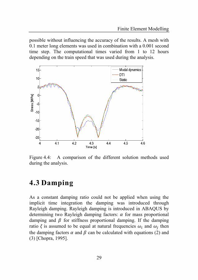
Finite Element Modelling
29
possible without influencing the accuracy of the results. A mesh with 0.1 meter long elements was used in combination with a 0.001 second time step. The computational times varied from 1 to 12 hours depending on the train speed that was used during the analysis.
Figure 4.4: A comparison of the different solution methods used during the analysis.
4.3 Damping
As a constant damping ratio could not be applied when using the implicit time integration the damping was introduced through Rayleigh damping. Rayleigh damping is introduced in ABAQUS by determining two Rayleigh damping factors: for mass proportional damping and for stiffness proportional damping. If the damping ratio is assumed to be equal at natural frequencies and then the damping factors and can be calculated with equations (2) and (3) [Chopra, 1995].

Finite Element Modelling
30
(2)
(3)
In order to determine the damping factors the damping ratio was chosen to be equal to 0.5% as recommended in Eurocode for these types of bridges. To ensure that the obtained results would be conservative the first natural frequency in equations (2) and (3) was set to be equal with the bridge first fundamental frequency and the second fundamental frequency was set to equal with the fundamental frequency of the studied stringer beams.
4.4 Loading
Moving concentrated forces were used to model the train loads. In order to model the moving train loads in ABAQUS a special MATLAB routine was used in order to create the load amplitude as a function of time. For each of the nodes that is located along the stringer beams and that is subjected to the loads a separate amplitude function was created. It has to be noted that if the amplitude functions of the all nodes are plotted, the sum of all the amplitudes at any point in time will be equal to amplitude of the total train load acting on the bridge. A more detailed description can be found at [Wallin, 2011]. The created amplitude functions were later written into ABAQUS input files. The routine used made it possible to create various amplitude functions for different train sets and speeds.
Finite Element Modelling
31
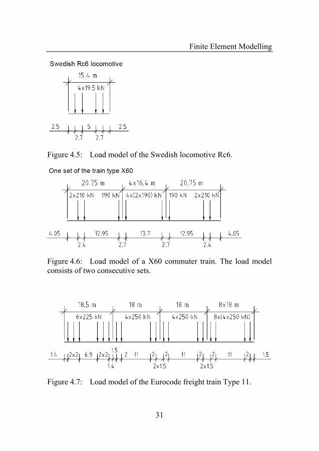
Figure 4.5: Load model of the Swedish locomotive Rc6.
Figure 4.6: Load model of a X60 commuter train. The load model consists of two consecutive sets.
Figure 4.7: Load model of the Eurocode freight train Type 11.

Finite Element Modelling
32
Three different types of train sets were used during the analysis. In order to compare the measured response with the results obtained during the analysis a standard Swedish locomotive RC6 (see figure 4.5) and a Swedish commuter train X60 (see figure 4.6) were used for the Söderstöm Bridge. To assess the fatigue damage created by the lighter commuter trains the Swedish commuter train X60 was used. To assess the influence of the heavier freight trains on the fatigue damage the heaviest train set that is proposed for fatigue assessment in the Eurocode, Type 11, was used (see figure 4.7). During the analysis only the western track of The Söderström Bridge was loaded.
In order to study the influence of different speeds, different analysis methods were used. At first the static response of the cross beams and the stinger beams were computed using static analysis. To study the impact that the different train speeds have on the accumulated fatigue, dynamic analyses were run using the direct time integration solution method. The studied speeds ranged from 10-120 km/h as high-speed train traffic is generally not allowed on open deck bridges.
In order to study the effect and the influence of the load distribution on the fatigue damage a longitudinal distribution of a point force that is proposed in the Eurocode was used (see figure 4.8). The effect was studied using train sets that crossed the models at a speed of 80 km/h. The same speed was used for investigating the cross beam effect.

Finite Element Modelling
33
Figure 4.8: The longitudinal distribution of a point force. Qvi is the point force that is subjected to the bridge by a single wheel. The distance between the sleepers is the distance marked with the letter a.
4.5 Comparison with measured results
4.5.1 The Söderström Bridge
The general behaviour of the model was checked by comparing the stress ranges in the corresponding cross-sections. The comparisons with the field measurement were carried out by comparing the stress ranges in the stringer beams section that is marked with a letter D in figure 5.7. The main reason why this cross-section is used during the comparison is that the measured signal, which was obtained during the measurement, was there the clearest. The stress range histories were obtained by applying the load distribution proposed in the Eurocode.

Finite Element Modelling
34
Figure 4.9: Stress history of the X60 train passage over the stringer beam at the speed of 80 km/h
Figure 4.10: Stress history of the RC6 locomotive passage over the stringer beam at the speed of 80 km/h
A good coherence was found when the stress range histories created by the passages of the X60 train and the Swedish RC6 locomotive were compared with the measured response (see figures 4.9 and

Finite Element Modelling
35
4.10). The passage of the RC6 locomotive shows a good general resemblance with the measured results although some differences in the peak values are still observed. However, the passage of the four more heavily loaded axels of the X60 train, which are placed in the middle of the train set, produced a stress range that resembled measured stress range accurately.
4.5.2 The Åby älv bridge
In the case of the Åby älv bridge the general behaviour of the model was checked by comparing the results from modal analysis with the measured and predicted natural frequencies and mode shapes. The comparison between the obtained natural frequencies for the first nine modes is presented in table 4.1. The model that was used in this research (3D beam model) proves to give accurate results compared to the advanced shell element model’s and the field measurement results. The advanced shell element model was created for predicting the mode shapes for an instrumentation programme for the dynamic testing of the Åby älv bridge [Andersson, 2013]. The mode shapes that were obtained for the 3D beam element model correspond well to the advance shell element model’s mode shapes (see figures 4.11 and 4.12).

Finite Element Modelling
36
Table 4.1: Natural frequencies: a comparison between measured results, advanced 3D shell model and 3D beam element model used in this study.
Figure 4.11: First three mode shapes obtained from modal analysis (3D beam model).
Figure 4.12: First three mode shapes obtained from 3D shell model [Andersson, 2013].
Mode no Measuredf [Hz]
3D shellf [Hz]
3D beamf [Hz]
1 3.7 4.0 4.4 2 7.4 7.6 8.1 3 8.8 9.0 9.2 4 9.1 9.7 9.8 5 10.2 10.5 10.6 6 11.4 11.4 11.4 7 13.8 14.0 12.2 8 16.2 16.5 13.5 9 17.3 16.8 15.9

Fatigue assessment
37
5
Fatigue assessment
5.1 Fatigue
Fatigue failure can be defined as the formation of a crack or cracks caused by repeatedly applied loads. Each of these loads are insufficient themselves to cause a normal static failure [Guerney, 1979]. Fatigue failure is created by a natural sequence of events that lead to the final failure of a structural element. The failure process (see figure 5.1) is initiated by a crack initiation that is followed by two stages of crack propagation. The two stages of fatigue crack growth are called “stage I” (shear mode) and “stage II” (tensile mode) [Forsyth, 1969]. The failure process ends with a final rupture of the structural element.
Chapter

Fatigue assessment
38
Figure 5.1: A schematic representation of crack growth as a function of the number of load cycles. The stages of failure are (1) initiation, (2) stage I crack growth (shear mode), (3) stage II crack growth, and (4) final rupture [Bickford, 2007].
Cracks always initiate in regions were natural stress raisers are present. These regions can be for example: section changes, inward corners, fillets, cuts, notches, holes, weld toes and weld roots. In such regions the crack is usually initiated near some microscopic defect like an inclusion or a void. These initial defects, as a form of section change, create stress concentrations which initiate the formation of micro cracks. The formation of micro cracks will lead to the formation of a macro crack. The tip of a crack is always very sharp which will cause extreme stress concentrations. The stresses at the tip mathematically reach to infinity if the theory of linear elastic material is assumed. However, stresses of this level are not possible in reality and the metal will yield at the crack tip. When the structural element is subjected to cyclic loads the crack tip continues to yield and tears the material at the root of the crack. Initial crack growth in stage I is generally very slow while most of the structural element remains undamaged. Fatigue crack propagation is controlled by shear stresses and propagation takes place under 45 degrees in relation to applied load. Stage I crack propagation is followed by Stage II crack propagations. Propagation in stage II is perpendicular to the load direction and controlled by maximum tensile stresses [Stephens, 2000]. At some point the crack has propagated so far that the element

Fatigue assessment
39
can only withstand a few more cycles. The crack propagation will go unstable as soon as the crack has reached this critical size. The final rupture or failure will occur within a few load cycles.
5.2 Stress concentrations
Cracks always initiate in regions with stress concentrations. Since early testing the detrimental effect of stress concentrations on fatigue strength has been shown. For example by Wöhler, who came to the conclusion, as a result of his classical experiments on railway axels, that sudden changes in diameter reduced the fatigue strength. His tests also show that the number of cycles that an axle can endure under a given applied stress spectra depends on the condition of the surface. A polished specimen survived much longer than the ones that were not polished [Guerney, 1979].
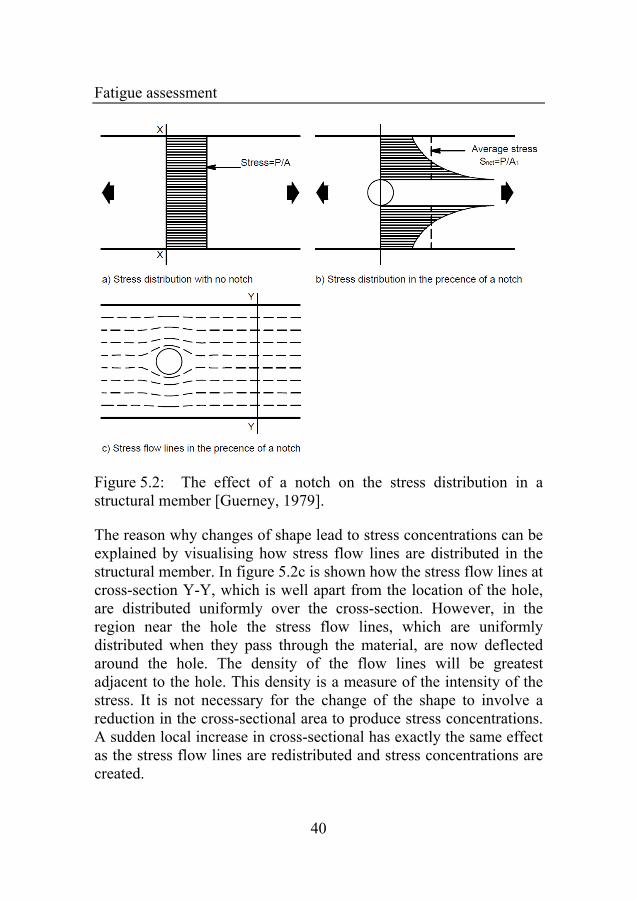
The influence of the stress concentrations created by notches and other discontinuities on the fatigue strength can be explained by the changes in stress distribution that these discontinuities create. The effect can be explained by comparing two structural members. If a smooth uniform plate is subjected to axial tensile load P the uniform stress distribution will have a value of P/A, when the cross-section has an area of A. (see figure 5.2a). When there is a hole in the otherwise identical plate the cross-sectional area will decrease to A1. The average stress will then increase to the value P/A1. Most significantly however, the stress distribution will change over the cross-section of the structural member. The stress distribution over the cross-section will no longer be uniform but will be of the general form shown in figure 5.2b. The stress at the edge of the hole is considerably higher than the average stress. Such stress peaks will be produced by any abrupt change of shape in a stressed structural member. These stress peaks are known as stress concentrations.
Fatigue assessment
40
Figure 5.2: The effect of a notch on the stress distribution in a structural member [Guerney, 1979].
The reason why changes of shape lead to stress concentrations can be explained by visualising how stress flow lines are distributed in the structural member. In figure 5.2c is shown how the stress flow lines at cross-section Y-Y, which is well apart from the location of the hole, are distributed uniformly over the cross-section. However, in the region near the hole the stress flow lines, which are uniformly distributed when they pass through the material, are now deflected around the hole. The density of the flow lines will be greatest adjacent to the hole. This density is a measure of the intensity of the stress. It is not necessary for the change of the shape to involve a reduction in the cross-sectional area to produce stress concentrations. A sudden local increase in cross-sectional has exactly the same effect as the stress flow lines are redistributed and stress concentrations are created.

Fatigue assessment
41
5.3 Fatigue evaluation according to Eurocode
5.3.1 S-N design curves
The Eurocode covering fatigue (EN 1993-1-9) presents a method to check fatigue resistance in case of high cycle fatigue (more than 10000 cycles). The method is used for checking the fatigue resistance of members, connections and joints that are subjected to fatigue loading. The method is based on a large number of S-N curves that are determined by testing specimens. Specimens that have been tested have different geometrical properties and structural imperfections. These imperfections cover defects that all structural elements have, for example structural imperfections formed during the material production or the effect of tolerances and residual stresses from welding. There are a total amount of 14 standardised S-N curves for the design procedure for direct stresses (see figure 5.3). For shear stresses only two standardized S-N curves are used. The S-N curves are valid to use only if the structural element under examination resembles the test specimens that are described in the code. The specimens in the code are characterized by a category number determined during testing. The S-N curves can be used directly if the detail is subjected to the constant stress range Δσ (see figure 5.4) during its entire life. From figure 5.3 three different limits can be distinguished. Δσc in the figure corresponds to a category number of the details described in the code and corresponds to the stress range that the detail can sustain for exactly 2 million cycles. Limit ΔσD=0.737Δσc (all cases set to 5 million cycles) represents the constant amplitude fatigue limit. It means that the structural detail under inspection can withstand an infinite number of load cycles if the detail is only under constant amplitude stress range that is lower than the limit during its entire lifetime. Stress ranges below the cut-off limit (ΔσL=0549ΔσD) are assumed not to contribute to the fatigue damage. In order to calculate the total number of cycles (N) that the

Fatigue assessment
42
structural part can handle equations (4) and (5) can be used instead of the actual graphs.∆ is the constant stress range that the structural element is subject to during the loading.
Figure 5.3: Fatigue strength curves for direct stress ranges. [EN-1993-1-9, 2006]
∆ ∆ 2 10 with m = 3 for 5 10 (4)
∆ ∆ 5 10 with m = 5 for 8 10 (5)

Fatigue assessment
43
5.3.2 Cycle counting methods
The S-N curves can only be used directly if the studied member is subjected to a constant amplitude stress range (see figure 5.4) during its entire design life. However, in reality the stress range history is usually more complicated (see figure 5.5a) and the stress range history consists of stress cycles that have different amplitudes. In order to carry out a fatigue assessment the stress ranges in the stress history have to be ordered into suitable sets of manageable intervals, in so called stress range spectrum histograms (see figure 5.6).
Figure 5.4: A constant amplitude stress history.
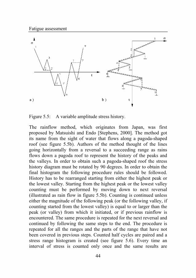
There are different techniques to obtain the size of the stress ranges that are part of the stress range spectrum. The methods suggested in the Eurocode are the rainflow method and the reservoir method. The rainflow method is more convenient when long and variable stress histories have to be analysed [Dwight, 1999].
Fatigue assessment
44
Figure 5.5: A variable amplitude stress history.
The rainflow method, which originates from Japan, was first proposed by Matsuishi and Endo [Stephens, 2000]. The method got its name from the sight of water that flows along a pagoda-shaped roof (see figure 5.5b). Authors of the method thought of the lines going horizontally from a reversal to a succeeding range as rains flows down a pagoda roof to represent the history of the peaks and the valleys. In order to obtain such a pagoda-shaped roof the stress history diagram must be rotated by 90 degrees. In order to obtain the final histogram the following procedure rules should be followed. History has to be rearranged starting from either the highest peak or the lowest valley. Starting from the highest peak or the lowest valley counting must be performed by moving down to next reversal (illustrated as rain flow in figure 5.5b). Counting is continued unless either the magnitude of the following peak (or the following valley, if counting started from the lowest valley) is equal to or larger than the peak (or valley) from which it initiated, or if previous rainflow is encountered. The same procedure is repeated for the next reversal and continued by following the same steps to the end. The procedure is repeated for all the ranges and the parts of the range that have not been covered in previous steps. Counted half cycles are paired and a stress range histogram is created (see figure 5.6). Every time an interval of stress is counted only once and the same results are

Fatigue assessment
45
obtained also in the case when the evaluation is proceeded in the opposite direction [Fryba, 1996].
Figure 5.6: a) Equivalent stress history obtained with the rainflow method. b) Stress range spectrum histogram
5.3.3 Fatigue life prediction
In order to perform the check of fatigue resistance of a structural member stresses should be calculated. In the EN 1993-1-9 there are three different approaches on how to calculate the stresses in the cross-section that are potentially most hazardous regarding fatigue damage. Each method has corresponding stress ranges. Nominal stress ranges are used when the code describes the examined section. Stress concentration effects are included when the right detail category is chosen. A stress in the examined section is calculated in the weld adjacent to a potential crack location in accordance with the elastic theory. Modified nominal stress ranges are used when the detail categories in the code are not describing geometrical changes. The influence of these geometrical changes that act like stress raisers are taken into account by multiplying the nominal stress by the stress concentration factors kf. The values of kf can be found in literature for the elementary cases or through finite element analysis [Guerney, 1979]. Geometrical stress ranges (hot spot stresses) are used when stress rising effects due to the overall geometry of a particular construction detail are not described in the code. They are most commonly used when the fatigue resistance of single welds are

Fatigue assessment
46
checked. The stresses (hot spot stresses) precisely at the weld toe are calculated with regard to global geometric effects in the examined weld connection. Geometrical effects of the weld itself are not included when the stresses are calculated.
In the case of a constant stress range failure criteria with partial coefficients are described with equations (6) and (7). The combined influence should be checked with equation (8)
∆ ∆ (6)
∆ ∆ (7)
∆
∆ /
∆
∆ /1.0 (8)
Fatigue resistance verification is carried out in the serviceability limit state for the variable loads that are described in EN 1990. When fatigue assessments are performed for bridges the dynamic amplification factor is given by equation (1) where and are defined with equations (9) and (12) [EN-1991-2]. The values of amplification factors are dependent on two parameters: and L. is the train speed in meters per second and L is the determinant length in meters in equations below.
′ (9)
for L 20 m (10)
. . for L 20 m (11)
′′ 0.56 (12)

Fatigue assessment
47
The determinant lengths are dependent on the type of structure and the type of structural element. The determinant lengths are defined in the tables in Eurocode.
Partial coefficient is the national choice in Sweden accounting for safety classes. is used as a partial coefficient on fatigue loads only. is a partial coefficient which is used for the fatigue resistance.
In the case of a variable stress range first the stress range has to be broken down to more manageable intervals, and then the stress range histogram is created (see figure 5.5b). The theory of fatigue damage accumulation is used [Palmgren, 1924]. In order to check the failure criterion for the variable stress range first the number of cycles (NRi) that would give fracture if a constant stress acts during the entire life of the structural element for each stress range in the histogram∆ …∆ need to be calculated. The following equations (13), (14), (15) should then be used.
∆
∆2 10 with m = 3
if ∆ ∆ (13)
∆
∆5 10 with m = 5
if ∆ ∆ ∆ (14)
∆
∆2 10 with m = 5
if ∆ ∆ (15)

Fatigue assessment
48
If the stress ranges ∆ or ∆ are smaller than the limits set in equations (14) and (15) then these stress ranges do not contribute to the total fatigue damage. After the number of cycles is calculated their influence to the total fatigue damage Dd is described and calculated sufficiently using the Palmgren-Miners rule [Fryba, 1996] with equation (16). ni is representing the number of cycles in corresponding stress range.
(16)
According to Eurocode damage occurs when 1
5.4 Fatigue assessment for the models
During the fatigue damage assessment nominal stress ranges were used. In order to obtain the nominal stress values from ABAQUS direct stresses of the node that is positioned closest to the critical section, were extracted. It is possible in ABAQUS to extract direct stress values from all critical section points of the examined critical cross-section. During the current assessment stresses in the corners of the I-profile sections were found. The stresses created by all section forces (bending moments and axial forces) are included in the direct stress (axial stress).

Fatigue assessment
49
Figure 5.7: Locations of the cross-sections examined during the fatigue damage assessment for the Söderström Bridge.
Figure 5.8: Locations of the cross-sections examined during the fatigue damage assessment for the Åby älv bridge.
In the case of the Söderstöm Bridge the stress ranges were obtained from the various locations that are placed over the model (see figure 5.7). The locations of the examined sections were chosen according to the previously conducted monitoring program that is shortly described in Chapter 2. The sections positioned in the middle of the span and next to the support were chosen at the position of the gauges that were installed during the monitoring program in order to compare the response of the model to the results obtained during the field measurements. In the case of the Åby älv bridge the stress ranges were studied at the midspans of the stringer beams (see figure 5.8) as the cross beams of the Åby älv bridge did not contain critical sections. The locations of the examined sections were chosen in the fatigue critical cross section were the highest stresses occur during train passages. The stress ranges were obtained from the several sections of the finite element model in order to ensure the quality of the results by avoiding errors during data processing.
In order to convert the extracted stress ranges into stress range spectrums the MATLAB routine named WAFO (Wave Analysis for Fatigue and Oceanography) developed at the Lund University was used. It is based on the rain-flow cycle counting method and is designed for statistical analysis and simulations of random waves and random loads. To obtain accurate results the stress histograms were computed using intervals with an accuracy of 1 MPa. The example of

Fatigue assessment
50
the input stress range and the routines output stress range histogram is shown in figures 5.9 and 5.10.
Figure 5.9: The stress range history created by the passage of the Type 11 train over the stinger beam at the speed of 80km/h
Figure 5.10: The stress range histogram based on the passage of the Type 11 train
The obtained stress range histograms were used during the fatigue damage calculations. The following partial coefficient values were used during the fatigue damage calculations: 1.0 for , 1.0 for and 1.35 for . These values are commonly used during fatigue assessments that are conducted for railway bridges. Equations (13), (14), (15) and (16) were used during the fatigue damage assessment.

Fatigue assessment
51
The accumulated damages in the critical sections for the bridges, which are marked red in figure 5.11 and 5.12, were computed during the assessment. The detail category in the Eurocode that corresponds to the critical sections that do not have a transitional radius is the category 40.
Figure 5.11: The critical sections for which the fatigue damage assessment was performed for the Söderström Bridge.
Figure 5.12: The critical sections for which the fatigue damage assessment was performed for the Åby älv bridge.


Results
53
6
Results
6.1 Influence of different train speeds
To study the influence of different speeds, the X60 and the Eurocode Type 11 train were used. To compute the accumulated damage according to the guidelines given in the Eurocode, the dynamic amplification factors calculated according to equation (1) were used. The values of the dynamic amplification factors varied from 1.05 to 1.21. The determinant length that was used for the stringer beams was 3 times the distance of the cross beam spacing and 2 times the length of the cross beams for the cross beams.
The accumulated damages obtained from dynamic analysis were normalised by dividing the calculated values by the corresponding static accumulated damage values. The same procedure was also used to normalize the dynamic accumulated fatigue damage found according to Eurocode. Only the most critical cross beam and stringer beam sections with the highest fatigue damage values were studied under variable speed conditions.
Chapter

Results
54
Figure 6.1: Accumulated relative damage under the load of a X60 train for the Söderström Bridge.
Figure 6.2: Accumulated relative damage under the load of a Type 11 train for the Söderström Bridge

Results
55
Figure 6.3: Accumulated relative damage under the load of Type 11 and X60 train for the stringer beam of the Åby älv bridge.
The results are presented in figures 6.1, 6.2 and 6.3. From these figures it can be seen that the influence of the dynamics on the accumulated fatigue damage does not change significantly with a change of speed. However, when the dynamic amplification factors are used (values vary from 1.05 to 1.21) as proposed in the Eurocode excessive accumulated damages are found. The use of these amplification factors produces the overestimated fatigue damages at higher speeds. In the case of the Söderström Bridge the most significant change can be found when cross beams are studied under the loading of the X60 train (see figure 6.1). The extensive differences are found due to the use of dynamic amplification factors which amplify static stress ranges. Cycles that would remain under the cut-off limit are included into the accumulated damage. In this specific case, these cycles, which were part of the S-N curve that is represented by equation (4), are moved into the part of the curve that is described with equation (5). Influence of both these factors results in highly overestimate fatigue damage, over 1.5 times at the lowest speed of 10km/h and over 2.1 times at the highest speed of 120km/h. For other cases the overestimation varies from 24% to 35% at the speed of 80 km/h and from 37% to 47% at the speed of 120 km/h.

Results
56
6.2 Influence of load distribution
The influence of the load distribution proposed in the Eurocode on the accumulated fatigue damage was calculated by comparing the accumulated damage created by the concentrated loading configurations with the damage created by the distributed load configurations.
Figure 6.4: Stress histories of the X60 train passages over the Söderström Bridge’s stringer beam with a speed of 80km/h modelled as concentrated and distributed point loads.
Clear differences were found in the stress ranges for the stringer beams for both train types (see table 6.1 and 6.2). An example is shown in figure 6.4. This resulted in a significant change in the accumulated fatigue damage. A decrease in the accumulated damage in the stringer beams of more than 20% can be achieved when the load distribution proposed in the Eurocode is used. The differences between the results for the two bridges can be explained by different span lengths. Larger reduction was obtained for the stringer beams of The Söderstöm Bridge that have shorter spans.

Results
57
Figure 6.5: Stress history of the Type 11 train passage over the Söderström Bridge’s cross beam at a speed of 80 km/h
The load distribution proposed in the Eurocode, however, does not have a significant effect on the accumulated damage in the cross beams. The small influence can be seen in figure 6.5, which illustrates only slight changes in the stress ranges. However, at least a 5% decrease in accumulated damage can be found at all critical sections for both train load models.
X60 Type 11
Support Midspan Support Midspan
Stringer beam 33.2% 35.9% 34.3% 35.3%
Cross beam 8.4% 11.9% 5.5% 6.7%
Table 6.1: Decrease in accumulated damaged in the result of load distribution for the Söderström Bridge.
X60 Type 11
Support Midspan Support Midspan
Stringer beam 24.2% 24.6% 26.3% 26.4%
Table 6.2: Decrease in accumulated damaged in the result of load distribution for the Åby älv bridge.

Results
58
6.3 Influence of the cross beam effect
The influence of the cross beam effect was investigated by studying the difference between the bridges responses under static and dynamic loading. The response was studied at a train speed of 80 km/h as different train speeds did not have an influence on the dynamic response (figure 6.1 to 6.3). The accumulated static and dynamic damages were calculated for different support stiffness conditions. The obtained results were normalised by dividing the dynamic damage by the static fatigue damage and were plotted against the stiffness ratio (modified structural system’s stiffness kfic and the original structural system’s stiffness k (figure 6.6 and 6.7). The fatigue damage was calculated at cross sections near the support (at D for The Söderström Bridge, at C for The Åby älv bridge) and at the midspan (at B for The Söderström Bridge, at B for The Åby älv bridge), see figure 5.7 and 5.8.
Figure 6.6: Accumulated relative damage under the load of the X60 and Type 11 trains for the stringer beams of the Söderström Bridge.

Results
59
Figure 6.7: Accumulated relative damage under the load of the X60 and Type 11 trains for the stringer beams of the Åby älv bridge.
Figures 6.6 and 6.7 show that no real reduction in the relative accumulated damage could be found. None of the studied sections showed any significant difference in statically and dynamically calculated damage.
The possible reduction of the accumulated fatigue damage was further studied by increasing the stiffness of various parts of the structural systems. As no fundamental difference was found in the behaviour between sections that are placed at the midspan of the bridge and near the support, only the results for the elements that place at the midspan are presented.
The accumulated damages were calculated for the systems with different stiffness modifications and then normalised by dividing the found fatigue damages by the original system’s accumulated fatigue damage. The results were plotted against the stiffness ratio (modified structural system’s stiffness kfic and the original structural system’s stiffness k), see figures 6.8 to 6.10. The results from the analysis with linear-elastic spring supports were related with the other modifications using the following methodology. At first, the models equivalent spring stiffness k was found by placing the point load on the simply supported cross beam and by calculating the spring stiffness from the displacement. The fictitious support stiffness kfic

Results
60
was found by summing the stiffness of the simply supported cross beam and a spring support.
The influence of the fatigue damage on different modifications is shown in graphs 6.8 and 6.9. The fatigue damages for the model whose main beams stiffness was increased are denoted with the abbreviation ‘MB’. The results for the model whose cross beams stiffness was increased are denoted with the abbreviation ‘CB’. The results for the model whose main and cross beam stiffness was increased are denoted with the abbreviation ‘MB+CB‘. The results for the analysis for the model with linear elastic supports are denoted with the abbreviation ‘Spring’.
Figure 6.8: Reduction of the accumulated fatigue damage in the stringer beams of the Söderström Bridge under the load of the X60 train.

Results
61
Figure 6.9: Reduction of the accumulated fatigue damage in the stringer beams of The Söderström Bridge under the load of the Type 11 train.
It is apparent in figure 6.8 and 6.9 that an increased stiffness of cross beams and main beams decreases the accumulated damage in the stringer. An added support structure, as the spring alternative represents, also decreases the damage. All the studied cases for The Söderstöm Bridge show that reduction in the fatigue damage is more significant when the structure is loaded with the X60 train than with the Type 11 train. More cycles are neglected for the X60 train because they are lower than the cut off limit. Also the cycles that are near the point of change on the S-N curve’s different slopes are moved to the point of the curve where the curves are described by the equation (5). This lowers the fatigue damage significantly. In these cases it is the loading of Type 11 trains that is creating higher stress cycles due to higher axial loads. However, these cycles are not lowered to that extent where they would shift in the way that they do in the case of the X60 loading.
The largest amount of reduction is achieved up until the point where the fictitious stiffness is about 6-8 times larger than the original stiffness. This is also the point where the fatigue damage reduction achieved using only spring supports approaches its maximum value (the fatigue damage’s further reduction is minimal when the stiffness of the linear elastic springs is increased). The additional reduction is caused by the methodology used for increasing the stiffness of the

Results
62
different elements. The modified Young’s modulus has also an influence on the rotational stiffness of the supports. The further reduction is therefore caused by increasing rotational stiffness.
Figure 6.10: Reduction of the accumulated fatigue damage in the cross beams as the result of the increased stiffness of the main beams for the Söderström Bridge.
The reduction in accumulated damage that is added from the stiffness increase of the main beams is relatively small for the stringer beams. The reduction in fatigue damage in the cross beams is more significant as can be seen from figure 6.10. Similar differences between different train types can be found as the reduction for the X60 is greater. The greatest amount of reduction is achieved up until the point where the fictitious stiffness is about 5 times the original stiffness. The further increase is caused by the increase of the rotational stiffness.

Results
63
Figure 6.11: Reduction of the accumulated fatigue damage in the stringer beams as the result of the increased stiffness of elastic spring supports for The Åby älv bridge.
The influence of the cross beam effect was studied using only spring supports in the case of the Åby älv bridge (see figure 6.11). The differences between the results of the X60 and Type 11 trains are small. Most of the reduction is achieved up to a stiffness ratio of 6. This is comparable with the fatigue reduction curve for the spring support in the case of the Söderström Bridge. It has to be noted that more result points in the beginning are plotted in figure 6.11 to illustrate the fact that the reduction in fatigue damage is not smooth. The curve has small jumps as the reduction in damage is influenced by the stress cycles redistribution.

Results
64

Discussion and conclusions
65
7
Discussion and conclusions
7.1 Discussion
Only beam and truss elements were used during the study which limited the way to describe the geometry of more complex connections that would have required the use of shell elements. Most of these connections are placed in the connection points of different elements. The cross beam connections to the main beam in figure 2.5 for example. These connections ensure that the elements work rigidly as assumed in structural calculations and in the finite element models used in this study. The comparisons with measured results presented in Section 5.4.1 and 5.4.2 show that the influence was reasonably small
It was decided to use only three different types of train load models. That could be considered as a serious limitation when it comes to dynamic analysis. However as the studied elements were short thick beams with high fundamental frequencies the influence of different axial distances is unlikely. By choosing the lighter passenger train load model and the heaviest freight train model in Eurocode the
Chapter

Discussion and conclusions
66
extremes of the loading profiles have been covered for the cross beam effect study in statics. While modelling the loads the suspension system of the train was not modelled and moving concentrated point loads were used. Track irregularities were also not taken into account during the modelling. That could be considered as a conservative approach when loading is modelled [Leander, 2013].
If the dynamic amplification factors are calculated based on the dynamic analysis using equation (17) (m=3), proposed in [Leander, 2013], the upper boundary value of 1.08 for cross beams was obtained. The upper boundary value for the stringer beams was 1.05. The obtained values are lower compared to the valued obtained using Eurocode (1.05 to 1.21).
/ / (17)
The overestimation of the fatigue damage at higher speeds when Eurocode’s approach is used indicates that the speed dependency in the equation (1) is questionable; a constant amplification factor should be used instead.
The cross beam effect in terms of dynamics for these two bridges was not detected. This can be the result of an initial high stiffness of the bridge deck. Which means that fundamental frequencies of the investigated elements are not affected by increased supports stiffness. The effect could not be detected also because of the chosen train speeds.
When the cross beam effect was studied in terms of statics it appeared that the range where the largest amount of reduction was achieved was when the stiffness of the supports (cross beams) was increased approximately 6-8 times. That type of reduction range was detected on both of the bridges. This is probably caused by the fact that both bridges were designed using the same design codes and the same loads. The cross beam effect in statics shows that the fatigue life of a

Discussion and conclusions
67
structure can be improved by increasing the support stiffness through strengthening.
The continuous beams that were used in this study had high fundamental frequencies and the cross beam effect was not detected. The studied beams also had height to length ratios which were larger than 0.1. The cross beam should be further studied in order to determine the fundamental frequency and the height to length ranges where the cross beam effect occurs and when it should be considered during the analysis.
7.2 Conclusions
In this thesis, 3D finite element models were used to investigate the influence of dynamic loading on fatigue damage on the examples of the Söderström Bridge and the Åby älv bridge. The general behaviour of the models was compared with field measurements and used in further studies. Different aspects that influence the fatigue damage were analysed using different train speeds and train sets. The influence of the dynamic loading on fatigue damage was studied and compared with the results obtained using Eurocode. The influence of the load distribution proposed in the Eurocode on fatigue damage was investigated. The cross beam effect was studied in terms of dynamics and statics. The following conclusions can be drawn based on the results:
Direct time integration based on implicit dynamic analysis step proved to be computationally more efficient and more accurate than the modal superposition solution method for short thick beams.
The use of the dynamic amplification factor proposed in the Eurocode overestimates fatigue damage at higher speeds and for all structural elements that were studied, more than to 24% at the speed of 80 km/h and more than 37% at the speed of 120 km/h for the case studies.

Discussion and conclusions
68
The use of the load distribution proposed in the Eurocode has larger influence on the damage for the stringer beams ,more than 20% for studied cases. For cross beams only a modest reduction in fatigue damage was found, up to 7%.
No dynamic amplification could be detected for the speeds that the open deck bridges are usually subjected to.
The influence of the cross beam effect has a significant influence on the fatigue damage in terms of statics. The cross beam effect is dependent on the train type.
Increased stiffness of the cross beams can reduce the accumulated damage of the stringers significantly, up to 48% for the case studies.

69
Bibliography
Andersson, A., 2009. Fatigue assessment of railway bridges. Licentiate thesis, Royal Institute of Technology, TRITA-BKN. Bulletin 96.
Andersson, A., Grip, N., 2013. Railway bridge over Åby älv. Instrumentation programme for dynamic testing. Technical report. KTH, August 6, 2013.
Bell, Brian, 2004. D1.2 European Railway Bridge Demography. Sustainable Bridges – Assessment for Future Traffic Demands and Longer Lives. www.sustainablebridges.net
Bickford, J. H., 2007. Introduction to the Design and Behavior of Bolted Joints, Fourth Edition. CRC Press, 2007,Ohio, USA. Chapter 15.
Brencich, A., Gambarotta, L., 2009. Assessment procedure and rehabilitation of riveted railway girders: The Campasso Bridge. Engineering Structures 31 (2009) 224-239.
Brühwiler, E., 2013. Fatigue safety examination of a 150-year old riveted railway bridge. Life-Cycle and Sustainability of Civil Infrastructure Systems – Strauss, Frangopol & Bergmeister.
Caglayan, B.O., Ozakgul, K., Tezer., O., 2009. Fatigue life evaluation of a through-girder steel railway bridge. Engineering Failure Analysis 16 (2009) 765–774.

BIBLIOGRAPHY
70
Chopra, A.K., 1995. Dynamics of Structures. Theory and Applications in Earthquake Engineering. Third Edition. Pearson Prentice Hall. New Jersey, US. Pages 456 and 457.
Dwight, J., 1999. Aluminium Design and Construction. E and FN Spon, London, UK. Chapter 12.
Ekelund, T., 2008. Rapport–särskild inspektion, Bro över Söderström, Ulriks-dal – Stuvsta, oförstörande provning av östra huvudbalken, livavstyvningar. Rapport 104032-2, Projektengagemang Anläggning i Stockholm AB.
EN 1991-2:2010. Eurocode 1: Actions on structures–Part 2: Traffic loads on bridges. European committee for standardization (CEN ). Brussels, Belgium.
EN 1993-1-9:2006. Eurocode 3: Design of steel structures- Part 1-9: Fatigue, European Committee for Standardisation (CEN), Brussels, Belgium.
Forsyth, P. J. E., 1969. The Physical Basis of Metal Fatigue, American Elsevier Publishing Co, New York
Frýba, L., 1996. Dynamics of railway bridges. Thomas Telford. London, UK. Pages 38-39, 204- 207 and 246.
Gurney, T. R., 1979. Fatigue of welded structures. CUP Archive, 1979, Pages 12-48.
Huanga, H., Chajes, M.J., Mertz, M.D., Shentonb, H. W., Kaliakin, V. N., 2002. Behavior of open steel grid decks for bridges. Journal of Constructional Steel Research 58 (2002) 819–842
Kaliyaperumal, G., Imam, B., Righiniotis, T., 2011. Advanced dynamic finite element analysis of a skew steel railway bridge. Engineering Structures, Volume 33, Issue 1, January 2011, Pages 181-190.

71
Leander, J., Karoumi, R., 2013. Dynamics of thick bridge beams and its influence on fatigue life predictions, Journal of Constructional Steel Research Volume 39, October 2013, Pages 262-271.
Leander, J., Andersson, A., Karoumi, R., 2010. Monitoring and enhanced fatigue evaluation of a steel railway bridge. Engineering Structures 2010; 32(3).
Leander, J., 2010. Improving a bridge fatigue life prediction by monitoring. Licentiate thesis, Royal Institute of Technology, TRITA-BKN. Bulletin 106.
Oehme, P., 1989 “Schäden an Stahltragwerken – eine Analyse (Damage Analysis of SteelStructures)”. IABSE Proceedings P-139/89.
Palmgren, A., 1924. Die Lebensdauer von Kugellagern. VDI Zeitschrift 68 (14).- Miner, M. A., 1945. Cumulative damage in fatigue. Journal of Applied Mechanics 12 (1).
Pettersson, N., 2010. Rapport–särskild inspektion 2010, Centralbron Söderström km 1+83, riktad visuell kontroll spann 3, in Swedish. Rapport 101255-3, Projektengagemang Anläggning i Stockholm AB.
Rönneberg, K., Hemdmark, I., 2010. The City Line in Stockholm, the longest three dimensional property unit in Sweden. http://www.gdmc.nl/3dcadastres/literature/3Dcad_2010_06.pdf
Sedlacek, G., Bijlaard, F., Géradin, M., Pinto, A., Dimova, S., 2008. Assessment of Existing Steel Structures: Recommendations for Estimation of Remaining Fatigue Life. Joint Research Centre, European Commission.
Stamatopoulos, G. N., 2013. Fatigue assessment and strengthening measures to upgrade a steel railway bridge. Journal of Constructional Steel Research 80 (2013) 346–354.
Stephens, R. I., Fatemi, A., Stephens, R. R., Fuchs, H. O., 2000. Metal fatigue in Engineering. Second Edition. A Wiley-Interscience Publication, New York, USA. Pages 33-56 and 282-291.

BIBLIOGRAPHY
72
Wallin, J., Leander, J., Karoumi, R., 2011. Strengthening of a steel railway bridge and its impact on the dynamic response to passing trains. Engineering Structures Volume 33, Issue 2, February 2011, Pages 635–646.
Zabel V, Schmidt A, Reichert I, Höll S. 2013. Monitoring of a riveted steel railway bridge. Life-Cycle and Sustainability of Civil Infrastructure Systems – Strauss, Frangopol & Bergmeister.