Duty-Cycled Wireless Sensor Networks: Wakeup Scheduling,Routing, and Broadcasting

Shouwen Lai

Dissertation submitted to the Faculty of theVirginia Polytechnic Institute and State University

in partial fulfillment of the requirements for the degree of

Doctor of Philosophyin

Computer Engineering

Binoy Ravindran, ChairPaul PlassmannY. Thomas HouAnil VullikantiYaling Yang

April 26, 2010Blacksburg, Virginia

Keywords: Wireless Sensor Network, Duty Cycle, MAC, Routing, Broadcast, Quorum SystemCopyright 2010, Shouwen Lai

Duty-Cycled Wireless Sensor Networks: Wakeup Scheduling, Routing andBroadcasting

Shouwen Lai

(ABSTRACT)

In order to save energy consumption in idle states, low duty-cycled operation is widely usedin Wireless Sensor Networks (WSNs), where each node periodically switches between sleepingmode and awake mode. Although efficient toward saving energy, duty-cycling causes many chal-lenges, such as difficulty in neighbor discovery due to asynchronous wakeup/sleep scheduling,time-varying transmission latencies due to varying neighbor discovery latencies, and difficulty onmultihop broadcasting due to non-simultaneous wakeup in neighborhood. This dissertation fo-cuses on this problem space. Specifically, we focus on three co-related problems in duty-cycledWSNs: wakeup scheduling, routing and broadcasting.

We propose an asynchronous quorum-based wakeup scheduling scheme, which optimizes het-erogenous energy saving ratio and achieves bounded neighbor discovery latency, without requiringtime synchronization. Our solution is based on quorum system design. We propose two designs:cyclic quorum system pair (cqs-pair) and grid quorum system pair (gqs-pair). We also presentfast offline construction algorithms for such designs. Our analytical and experimental results showthat cqs-pair and gqs-pair achieve better trade-off between the average discovery delay and energyconsumption ratio. We also study asymmetric quorum-based wakeup scheduling for two-tierednetwork topologies for further improving energy efficiency.

Heterogenous duty-cycling causes transmission latencies to be time-varying. Hence, the routingproblem becomes more complex when the time domain must be considered for data delivery induty-cycled WSNs. We formulate the routing problem as time-dependent Bellman-Ford problem,and use vector representation for time-varying link costs and end-to-end (E2E) distances. Wepresent efficient algorithms for route construction and maintenance, which have bounded time andmessage complexities in the worst case by ameliorating with β-synchronizer.

Multihop broadcast is complex in duty-cycled WSNs due to non simultaneous wakeup in neighbor-hoods. We present Hybrid-cast, an asynchronous multihop broadcast protocol, which can be ap-plied to low duty-cycling or quorum-based duty-cycling schedules, where nodes send out a beaconmessage at the beginning of wakeup slots. Hybrid-cast achieves better tradeoff between broadcastlatency and broadcast count compared to previous broadcast solutions. It adopts opportunistic datadelivery in order to reduce the broadcast latency. Meanwhile, it reduces redundant transmissionvia delivery deferring and online forwarder selection. We analytically establish the upper bound ofbroadcast count and the broadcast latency under Hybrid-cast.

To verify the feasibility, effectiveness, and performance of our solutions for asynchronous wakeupscheduling, we developed a prototype implementation using Telosb and TinyOS 2.0 WSN plat-forms. We integrated our algorithms with the existing protocol stack in TinyOS, and comparedthem with the CSMA mechanism. Our implementation measurements illustrate the feasibility,performance trade-off, and effectiveness of the proposed solutions for low duty-cycled WSNs.

This work was supported by the Ministry of Knowledge Economy (MKE) of the Republic ofKorea. [2008-F-052, Scalable/Mobile/Reliable Wireless Sensor Network Technology].

iii

To my parents and my wife (Jinyan)

iv

Acknowledgments

After staying at Virginia Tech for three years, I am pleased to have reached this step. In the pastyears, many times I felt frustrated and pressured. I am lucky to get through all those difficultieswith the help and support from many people, and I would like to thank them.

First of all, I would like to thank my advisor, Dr. Binoy Ravindran. He offered me the chanceof working with him from my first day at Virginia Tech. Thanks for his advice and support inthe initial stage of my PhD when I was weak to start research in the Real-time Systems Labora-tory. I learned a lot from him on academic writing, presentations, and selecting correct researchdirections. He always encouraged me to do research of the highest quality even when I sufferedset-backs at first. I also highly appreciate his faith in me, allowing me to select my favorite researchdirections in these years.

Thanks, too, to the rest of my committee: Dr. Tom Hou, Dr. Paul Plassmann, Dr. Anil Vullikanti,and Dr. Yaling Yang. I greatly appreciate their support and encouragement on my work, andalso their willingness to bend their schedules to accommodate the meetings and exams. I am alsograteful to Dr. Hyeonjoong Cho, who is an alumni of my laboratory and now works at KoreaUniversity. He offered me many suggestions and comments when I prepared my first conferencepaper. I also thank him for securing the financial support from ETRI, Korea, which supported mydissertation research.

In addition, I would like to thank all my colleagues in the Real-Time Systems Laboratory whodiscussed with me many valuable ideas of my research. They include Kai Han, Jonathan Anderson,Bo Jiang, Bo Zhang, Guanhong Pei, Fei Huang, Sherif Fahmy, Piyush Garyali, and Junwhan Kim.I am also grateful to all my friends at VT for helping me in innumerable ways, especially for thoseserving with me in VT-ACSS, GSA Research Symposium, and BSO Budget Board.

Lastly, I would like to thank my family members for all their love and support. I am grateful to myparents for their hard work which allowed me to afford my education from when I was a child towhen I became a college student. Without their love, I would not have reached this milestone andthis dissertation would not have happened. I would like to thank especially my elder brother whois always a role model for me, inspiring me as I was growing up. Finally, I am forever indebted tomy wife Jinyan Fu. She has been incredibly supportive of me through the ups and downs over thepast years. I cannot thank her enough for being such a wonderful wife.

This dissertation is to all people who have helped and are helping me.

v

Contents

1 Introduction 1

1.1 Duty-cycled Wireless Sensor Networks . . . . . . . . . . . . . . . . . . . . . . . 2

1.2 Problem Spaces and Motivations . . . . . . . . . . . . . . . . . . . . . . . . . . . 3

1.3 Summary of Research Contributions . . . . . . . . . . . . . . . . . . . . . . . . . 5

1.4 Organization . . . . . . . . . . . . . . . . . . . . . . . . . . . . . . . . . . . . . . 8

2 Past and Related Works 9

2.1 Low Duty-Cycling MAC Protocols . . . . . . . . . . . . . . . . . . . . . . . . . . 9

2.1.1 LPL/ALPL mode . . . . . . . . . . . . . . . . . . . . . . . . . . . . . . . 9

2.1.2 Slotted Listening Mode . . . . . . . . . . . . . . . . . . . . . . . . . . . . 10

2.2 Neighbor Discovery Mechanisms over Duty-Cycled WSNs . . . . . . . . . . . . . 10

2.2.1 On-Demand neighbor discovery . . . . . . . . . . . . . . . . . . . . . . . 10

2.2.2 Synchronized neighbor discovery . . . . . . . . . . . . . . . . . . . . . . 11

2.2.3 Asynchronous neighbor discovery . . . . . . . . . . . . . . . . . . . . . . 12

2.3 Routing over Duty-cycled WSNs . . . . . . . . . . . . . . . . . . . . . . . . . . . 13

2.3.1 Opportunistic Routing . . . . . . . . . . . . . . . . . . . . . . . . . . . . 13

2.3.2 Deterministic Routing . . . . . . . . . . . . . . . . . . . . . . . . . . . . 14

2.4 Broadcast over Duty-Cycled WSNs . . . . . . . . . . . . . . . . . . . . . . . . . 15

2.4.1 Gossip or Opportunistic Approach . . . . . . . . . . . . . . . . . . . . . . 15

2.4.2 Synchronized or Duty-cycle Awareness . . . . . . . . . . . . . . . . . . . 15

2.4.3 Asynchronous Mechanisms . . . . . . . . . . . . . . . . . . . . . . . . . 16

vi

3 Preliminaries, Assumptions and Problem Statement 17

3.1 Network Model and Assumptions . . . . . . . . . . . . . . . . . . . . . . . . . . 17

3.2 Quorum-based wakeup scheduling . . . . . . . . . . . . . . . . . . . . . . . . . . 18

3.2.1 Quorum Systems . . . . . . . . . . . . . . . . . . . . . . . . . . . . . . . 18

3.2.2 Quorum-based Power Saving . . . . . . . . . . . . . . . . . . . . . . . . . 19

3.3 Neighbor Discovery Mechanism with LPL mode . . . . . . . . . . . . . . . . . . 20

3.4 Chinese Remainder Theorem . . . . . . . . . . . . . . . . . . . . . . . . . . . . . 21

3.5 Problem Statement and Goals . . . . . . . . . . . . . . . . . . . . . . . . . . . . . 21

3.5.1 Heterogeneous Quorum-Based Wakeup Scheduling . . . . . . . . . . . . . 21

3.5.2 Time-Dependent Bellman-Ford Equation . . . . . . . . . . . . . . . . . . 22

3.5.3 Hybrid Broadcast . . . . . . . . . . . . . . . . . . . . . . . . . . . . . . . 23

4 Asynchronous Wakeup Scheduling 24

4.1 Heterogenous Quorum-based Wakeup Scheduling . . . . . . . . . . . . . . . . . . 24

4.1.1 Heterogeneous Rotation Closure Property . . . . . . . . . . . . . . . . . . 24

4.1.2 Cyclic Quorum System Pair: cqs-pair . . . . . . . . . . . . . . . . . . . . 26

4.1.3 Grid Quorum System Pair: gqs-pair . . . . . . . . . . . . . . . . . . . . . 28

4.1.4 Construction Scheme for cqs-pair . . . . . . . . . . . . . . . . . . . . . . 28

4.1.5 Performance Analysis . . . . . . . . . . . . . . . . . . . . . . . . . . . . 32

4.1.6 Simulation Results . . . . . . . . . . . . . . . . . . . . . . . . . . . . . . 35

4.1.7 Conclusions . . . . . . . . . . . . . . . . . . . . . . . . . . . . . . . . . . 39

4.2 Asymmetric Quorum-based Wakeup Scheduling . . . . . . . . . . . . . . . . . . . 39

4.2.1 Motivations . . . . . . . . . . . . . . . . . . . . . . . . . . . . . . . . . . 39

4.2.2 Protocol Design of p-Grid . . . . . . . . . . . . . . . . . . . . . . . . . . 40

4.2.3 Performance Analysis . . . . . . . . . . . . . . . . . . . . . . . . . . . . 46

4.2.4 Experimental Results . . . . . . . . . . . . . . . . . . . . . . . . . . . . . 50

4.2.5 Conclusions and Discussions . . . . . . . . . . . . . . . . . . . . . . . . . 55

5 Routing over Heterogenous Wakeup Scheduling 57

vii

5.1 Motivations . . . . . . . . . . . . . . . . . . . . . . . . . . . . . . . . . . . . . . 57

5.2 Problem Formulations . . . . . . . . . . . . . . . . . . . . . . . . . . . . . . . . 59

5.3 Modeling Adaptively Duty-cycled WSNs . . . . . . . . . . . . . . . . . . . . . . 60

5.3.1 Link Cost Function . . . . . . . . . . . . . . . . . . . . . . . . . . . . . . 60

5.3.2 Distance to Sink . . . . . . . . . . . . . . . . . . . . . . . . . . . . . . . 61

5.3.3 Implementation via Vectors . . . . . . . . . . . . . . . . . . . . . . . . . 63

5.3.4 Properties . . . . . . . . . . . . . . . . . . . . . . . . . . . . . . . . . . . 65

5.4 Algorithm for Initial Route Construction . . . . . . . . . . . . . . . . . . . . . . . 66

5.4.1 Distributed Algorithm Description . . . . . . . . . . . . . . . . . . . . . . 66

5.4.2 Correctness and Complexity . . . . . . . . . . . . . . . . . . . . . . . . . 68

5.5 Algorithm for Dynamic Route Maintenance . . . . . . . . . . . . . . . . . . . . . 69

5.5.1 Distributed Algorithm Descriptions . . . . . . . . . . . . . . . . . . . . . 70

5.5.2 Correctness and Complexity . . . . . . . . . . . . . . . . . . . . . . . . . 73

5.5.3 Sub-optimal Implementation with Vector Compression . . . . . . . . . . . 74

5.5.4 Further Discussions . . . . . . . . . . . . . . . . . . . . . . . . . . . . . . 75

5.6 Experimental Results . . . . . . . . . . . . . . . . . . . . . . . . . . . . . . . . . 75

5.6.1 Least-latency Path Construction . . . . . . . . . . . . . . . . . . . . . . . 77

5.6.2 Least-latency Path Maintenance . . . . . . . . . . . . . . . . . . . . . . . 78

5.6.3 Performance of Sub-Optimal Implementation . . . . . . . . . . . . . . . . 79

5.7 Discussions . . . . . . . . . . . . . . . . . . . . . . . . . . . . . . . . . . . . . . 80

5.8 Conclusions . . . . . . . . . . . . . . . . . . . . . . . . . . . . . . . . . . . . . . 82

6 Broadcast over Duty-Cycled WSNs 83

6.1 Motivations and Goals . . . . . . . . . . . . . . . . . . . . . . . . . . . . . . . . 83

6.2 Hybrid-cast Protocol . . . . . . . . . . . . . . . . . . . . . . . . . . . . . . . . . 84

6.2.1 Overview . . . . . . . . . . . . . . . . . . . . . . . . . . . . . . . . . . . 84

6.2.2 Wakeup Schedule Switching . . . . . . . . . . . . . . . . . . . . . . . . . 85

6.2.3 Opportunistic Forwarding with Deferring . . . . . . . . . . . . . . . . . . 85

6.2.4 Online Forwarder Selection . . . . . . . . . . . . . . . . . . . . . . . . . 86

viii

6.3 Performance Analysis . . . . . . . . . . . . . . . . . . . . . . . . . . . . . . . . . 88

6.3.1 Upper-Bound on One-Hop Broadcast Count . . . . . . . . . . . . . . . . . 88

6.3.2 Delivery Latency . . . . . . . . . . . . . . . . . . . . . . . . . . . . . . . 89

6.4 Simulation Results . . . . . . . . . . . . . . . . . . . . . . . . . . . . . . . . . . 89

6.4.1 Broadcast Count . . . . . . . . . . . . . . . . . . . . . . . . . . . . . . . 89

6.4.2 Broadcast Latency . . . . . . . . . . . . . . . . . . . . . . . . . . . . . . 90

6.4.3 Impact of Network Size . . . . . . . . . . . . . . . . . . . . . . . . . . . 91

6.5 Discussions and Conclusions . . . . . . . . . . . . . . . . . . . . . . . . . . . . . 92

7 Prototype Implementations 93

7.1 Hardware and Software Platform . . . . . . . . . . . . . . . . . . . . . . . . . . . 93

7.2 Protocol Stacks and Modules . . . . . . . . . . . . . . . . . . . . . . . . . . . . . 95

7.3 Implementations of cqs-pair and gqs-pair . . . . . . . . . . . . . . . . . . . . . . 96

7.3.1 Beacon Messages . . . . . . . . . . . . . . . . . . . . . . . . . . . . . . . 96

7.3.2 Power Management . . . . . . . . . . . . . . . . . . . . . . . . . . . . . 97

7.3.3 Support for Multicast and Broadcast . . . . . . . . . . . . . . . . . . . . . 98

7.4 Demo Performance . . . . . . . . . . . . . . . . . . . . . . . . . . . . . . . . . . 99

8 Conclusions and Future Work 101

8.1 Summary of Contributions . . . . . . . . . . . . . . . . . . . . . . . . . . . . . . 103

8.2 Future Work . . . . . . . . . . . . . . . . . . . . . . . . . . . . . . . . . . . . . . 104

ix

List of Figures

1.1 Typical Multihop WSN Architecture . . . . . . . . . . . . . . . . . . . . . . . . . 1

1.2 Duty-cycled operation in WSNs . . . . . . . . . . . . . . . . . . . . . . . . . . . 2

3.1 Cyclic Quorum System (left) and Grid Quorum System (right) . . . . . . . . . . . 19

3.2 Neighbor discovery under partial overlap . . . . . . . . . . . . . . . . . . . . . . . 20

3.3 Neighbor discovery mechanism with periodic LPL scheduling in the X-MAC pro-tocol . . . . . . . . . . . . . . . . . . . . . . . . . . . . . . . . . . . . . . . . . . 20

4.1 Heterogenous rotation closure property between two cyclic quorum systems: Awith cycle length of 7 and B with cycle length of 21. A quorum from A’s p-extension Ap will overlap with a quorum from B. . . . . . . . . . . . . . . . . . . 25

4.2 Two quorums do not satisfy heterogenous rotation closure property although theyare from cyclic quorum systems respectively. . . . . . . . . . . . . . . . . . . . . 26

4.3 An example grid quorum system pair and its rotation closure property: grid quorumsystem A has a grid 4× 4 and B has a grid 6× 6. A quorum from A and a quorumfrom B overlap at 3 slots with B’s cycle length. . . . . . . . . . . . . . . . . . . . 28

4.4 Quorum Ratio and Average Discovery Delay for Cyclic Quorum Systems (Numer-ical Results) . . . . . . . . . . . . . . . . . . . . . . . . . . . . . . . . . . . . . . 36

4.5 Quorum Ratio and Average Discovery Delay for Grid Quorum Systems (Numeri-cal Results) . . . . . . . . . . . . . . . . . . . . . . . . . . . . . . . . . . . . . . 36

4.6 Impact of Heterogeneity . . . . . . . . . . . . . . . . . . . . . . . . . . . . . . . 37

4.7 Impact of Traffic Load: Energy Consumption Ratio . . . . . . . . . . . . . . . . . 38

4.8 Impact of Traffic Load: average discovery delay . . . . . . . . . . . . . . . . . . . 38

4.9 Two operation modes and neighbor discovery procedure in p-Grid . . . . . . . . . 41

x

4.10 Intersection between a write quorum and a read quorum from two prime-grid quo-rum groups: the write quorum A from the grid quorum group Q3×3, and the readquorum B from the grid quorum groupQ5×5. A2

⋂B �= ∅ . . . . . . . . . . . . . 44

4.11 An example of the intersection between a big read quorum and a small write quo-rum. Case 1: intersection within the first n slots of A; case 2: intersection beyondthe first n slots of A. . . . . . . . . . . . . . . . . . . . . . . . . . . . . . . . . . 49

4.12 Energy Consumptions: reliable environment (left); unreliable environment withnode failure probability being 0.3(right) . . . . . . . . . . . . . . . . . . . . . . . 52

4.13 One-hop discovery latency between a read quorum and write quorum from thesame grid quorum group Q5×5 . . . . . . . . . . . . . . . . . . . . . . . . . . . . 52

4.14 Average neighbor discovery latency for asymmetric design: (m, m)− > (n, n)represents the discovery latency between a node equipped with write quorum fromQm×m and a node equipped with read quorum fromQn×n . . . . . . . . . . . . . 53

4.15 Neighbor discovery ratio: a). different protocols; b). different failure ratios . . . . . 54

5.1 Varying neighbor discovery latency in heterogenous LPL mode . . . . . . . . . . . 61

5.2 Example for vector implementation . . . . . . . . . . . . . . . . . . . . . . . . . 64

5.3 Triangular path condition: the direct one-hop path ni → nj always achieve theleast latency among all pathes from ni to nj. . . . . . . . . . . . . . . . . . . . . . 66

5.4 Quorum duty-cycling: detector with the quorum from (21,5,1)-difference set de-sign, and neighbors with quorum from (7,3,1)-difference set design, as presentedin [1]. . . . . . . . . . . . . . . . . . . . . . . . . . . . . . . . . . . . . . . . . . 76

5.5 Comparison of time efficiency and message efficiency by varying |V | . . . . . . . 77

5.6 Comparison of time efficiency and message efficiency by varying time slots inALPL mode . . . . . . . . . . . . . . . . . . . . . . . . . . . . . . . . . . . . . . 77

5.7 Comparison of time efficiency and message efficiency for quorum-based duty-cycle setting . . . . . . . . . . . . . . . . . . . . . . . . . . . . . . . . . . . . . . 78

5.8 Performance comparison for route maintenance by varying input change: ALPLmode . . . . . . . . . . . . . . . . . . . . . . . . . . . . . . . . . . . . . . . . . 79

5.9 Performance comparison for route maintenance on memory required in each node . 79

5.10 Performance comparison for route construction: latency and vector size over ALPLmode . . . . . . . . . . . . . . . . . . . . . . . . . . . . . . . . . . . . . . . . . 80

5.11 Performance comparison for route construction: latency and message size overquorum-based duty-cycling mode . . . . . . . . . . . . . . . . . . . . . . . . . . 80

xi

5.12 Varying neighbor discovery delay for quorum wakeup scheduling . . . . . . . . . . 81

6.1 Opportunistic broadcasting with delivery deferring (a) low duty-cycling case; (b)quorum duty-cycling case with wakeup schedules of [1,1,0,1,0,0,0] and its rota-tions which comply with (7,3,1) cqs design in [1]. . . . . . . . . . . . . . . . . . . 85

6.2 Online forwarder selection and the triangular path condition. . . . . . . . . . . . . 87

6.3 Performance comparison on broadcast count . . . . . . . . . . . . . . . . . . . . . 90

6.4 Performance comparison on broadcast latency . . . . . . . . . . . . . . . . . . . . 90

6.5 Broadcast count with different network size. . . . . . . . . . . . . . . . . . . . . . 91

6.6 Broadcast latency with different network size. . . . . . . . . . . . . . . . . . . . . 91

7.1 Telosb and System Architecture in Implementations . . . . . . . . . . . . . . . . . 94

7.2 Monitoring GUI on PC . . . . . . . . . . . . . . . . . . . . . . . . . . . . . . . . 95

7.3 Protocols stacks in the prototype system . . . . . . . . . . . . . . . . . . . . . . . 96

7.4 Power Management at the Transmitter Side: Communication Schedule and Wakeupschedule . . . . . . . . . . . . . . . . . . . . . . . . . . . . . . . . . . . . . . . . 97

7.5 Performance Comparison for Line Topology . . . . . . . . . . . . . . . . . . . . . 99

7.6 Performance Comparison for Tree Topology . . . . . . . . . . . . . . . . . . . . . 99

xii

List of Tables

1.1 Energy consumption of different components in Telosb . . . . . . . . . . . . . . . 2

4.1 cqs-pair (for n, m ≤ 21) . . . . . . . . . . . . . . . . . . . . . . . . . . . . . . . 33

5.1 Network Size Sets . . . . . . . . . . . . . . . . . . . . . . . . . . . . . . . . . . . 76

5.2 Time slot sets . . . . . . . . . . . . . . . . . . . . . . . . . . . . . . . . . . . . . 76

xiii

Nomenclature

ALPL adaptive low power listing, page 11

ATIM Ad hoc Traffic Indication Map, page 97

cqs-pair cyclic quorum system-pair, page 6

CSMA Carrier Sense Multiple Access, page 4

E2E End-to-End, page 7

FIFO First-In-First-Out, page 59

FTSP fast time-dependent shortest path, page 67

FTSP-M fast maintenance algorithm for time-dependent shortest path, page 70

gqs-pair grid quorum system pair, page iii

h-QPS heterogeneous quorum-based power saving, page 22

LCM least common multiple , page 75

LPL low power listening, page 3

MCDS minimum connecting dominating set, page 87

MPR multipoint relays, page 88

p-Grid prime grid quorum system, page 7

QPS quorum-based power saving, page 4

S-MAC Sensor-MAC, page 4

TDSP time-dependent shortest path, page 59

WSN Wireless Sensor Networks, page 2

xiv

Chapter 1

Introduction

Wireless Sensor Networks (WSN ) consist of spatially distributed autonomous sensor nodes whichare organized into a cooperative network [2]. WSNs are usually deployed to monitor physicalor environmental properties, such as temperature, vibration, pressure, motion, or pollutants. Thedevelopment of WSNs was initially motivated by military applications such as battlefield surveil-lance. However, they are increasingly being used in many industrial and civilian application do-mains, including industrial process monitoring and control [3], machine health monitoring [4],environment and habitat monitoring [5], and medical diagnostics [6].

In WSNs, each node consists of a micro-processor, multiple types of memory (program, data andflash memories), RF transceiver, various sensors and actuators, and power supplies (e.g., batteriesand solar cells). A WSN normally constitutes a wireless ad-hoc network, meaning that each sensornode supports a multihop routing algorithm, and several nodes may forward data packets to a basestation via a sink node. A typical multihop architecture for WSNs is shown in Figure 1.1.

Base Station

Sink Node/Gateway

Sensor Node

Figure 1.1: Typical Multihop WSN Architecture

1

2

A sensor node is usually constrained by small size and low cost [7]. Such constraints affect thedesign of power supplies, memory, computational speed, and bandwidth. In particular, sensornodes usually rely on portable power sources such as batteries to provide the necessary power.Thus, energy efficiency is critically important for WSNs [2].

1.1 Duty-cycled Wireless Sensor Networks

It has been observed that idle energy plays an important role for saving energy in WSNs [8]. Mostexisting radios (i.e., CC2420 [9]) used in WSNs support different modes, such as transmit/receivemode, idle mode, and sleep mode. In the idle mode, the radio is not communicating but the radiocircuitry is still turned on, resulting in energy consumption which is only slightly less than thatin the transmitting or receiving states. Thus, a better way is to shut down the radio as much aspossible in the idle mode [8]. The typical energy consumption parameters for a Telosb [10] areshown in Table 1.1

Table 1.1: Energy consumption of different components in TelosbModule Power Remarks

Processor/memory 1.8 mA Active modeProcessor/memory 5.1 μA Sleep modeRadio RX mode 18.8 mA receivingRadio TX mode 17.4 mA transmissionRadio Idle mode 21 μA

Radio Sleep mode 1 μA

Suppose time is arranged into consecutive and equal time slots. Now, two modes for low duty cycleoperation can be identified: slotted listening mode [11, 12] and low power listening mode [13]. Inthe slotted listening mode, as shown in Figure 1.2(a), a node is wholly awake in select slots andasleep in the remaining slots when there is no data transmission or reception. In the low powerlistening (LPL ) mode, as shown in Figure 1.2(b), a node will be fractionally awake in every slot.

Sender

Receiver

wakeuptime slot

S

R

(a) Slotted listening

Sender

Receiver

wakeuptime slot

S

R

(b) Low power listening

Figure 1.2: Duty-cycled operation in WSNs

We define duty cycle as the percentage of time a node is active in the whole operational time.Generally, the duty cycle in the LPL mode is lower than that in the slotted listening mode.

3

Adaptive duty-cycling has been proposed in the recent works on energy-harvesting technolo-gies [14,15], such as solar power [16], to replenish battery supply in WSNs. Due to high costs andthe unavailability of a continuous power supply, it is not feasible to have instantly sufficient energyoutput. Hence, saving idle energy consumption is still necessary. Adaptive duty cycling [15,17] isthus proposed to save energy consumption and to prolong the sustainable workable time per node.The duty cycle setting can be based on the residual energy [18], node location, or the rechargeableenergy [17] on each node, independently.

Although low and adaptively duty-cycled operations can yield greater energy efficiency for WSNs,neighbor discovery becomes more complex than that in conventional works for always-on mecha-nisms (e.g., CSMA ), since we cannot guarantee that two nodes are awake simultaneously.

1.2 Problem Spaces and Motivations

To support duty cycling, it is necessary to introduce a wakeup scheduling scheme in which a nodesleeps in more slots in idle state, but maintains network connectivity. Towards this goal, existingneighbor discovery mechanisms fall into three categories: on-demand wakeup, scheduled neighbordiscovery, and asynchronous neighbor discovery.

In on-demand wakeup mechanisms [19–22], out-of-band signaling or operational cycle is used towake up sleeping nodes in an on-demand manner. For example, with the help of a paging signal, anode listening on a page channel can be awakened. As page radios can operate at lower power con-sumption, this strategy is very energy efficient. However, it suffers from increased implementationcomplexity.

In scheduled wakeup mechanisms [23–25], low-power sleeping nodes wake up at the same time,periodically, to communicate with one another. Examples include the S-MAC protocol [23] andthe multi-parent schemes protocol [26]. In such schemes, all nodes maintain periodic sleep-listenschedules based on locally managed synchronization. Neighboring nodes form virtual clusters toset up a common sleep schedule.

The third category, asynchronous wakeup mechanisms [12,13,27–29] are also well studied. Com-pared to the scheduled neighbor discovery wakeup mechanism, asynchronous wakeup does notrequire clock synchronization. In this approach, each node follows its own wakeup schedule inthe idle state, as long as the wakeup intervals among neighbors overlap. To meet this require-ment, nodes usually have to wakeup more frequently than in the scheduled neighbor discoverymechanism. However, there are many advantages of asynchronous wakeup, such as easiness inimplementation and low message overhead for communication. Furthermore, it can ensure net-work connectivity even in highly dynamic networks.

The quorum-based wakeup scheduling paradigm, sometimes called quorum-based power saving(QPS) protocol [11, 30–32], is an asynchronous wakeup mechanism in slotted listening mode,and has been proposed as a powerful solution for asynchronous wakeup scheduling. In a QPS

4

protocol, the time axis on each node is evenly divided into beacon intervals. Given an integer n, aquorum system defines a cycle pattern, which specifies the awake/sleep scheduling pattern duringn continuous beacon intervals for each node. We call n the cycle length, since the pattern repeatsevery n beacon intervals. A node may stay awake or sleep during each beacon interval. QPSprotocols guarantee that at least one awake interval overlaps between two adjacent nodes, witheach node being awake for only O(

√n) beacon intervals.

Most previous works only consider homogenous quorum systems for asynchronous wakeup schedul-ing [12], which means that quorum systems for all nodes have the same cycle length and samepattern. However, many WSNs are increasingly heterogenous in nature—i.e., the network nodesare grouped into clusters, with each cluster having a high-power cluster head node and low-powercluster member nodes [33–38].

Thus, the first problem that we focus in this dissertation is heterogenous quorum systems de-sign, where heterogenous sensor nodes (i.e., clusterheads and cluster members) have differentquorum-based wakeup schedules (or different cycle lengths). We denote two quorums from dif-ferent quorum systems as heterogenous quorums in this dissertation. If two adjacent nodes adoptheterogenous quorums as their wakeup schedules, they have different cycle lengths and differentwakeup patterns. Hence, how to guarantee the intersection property for heterogenous quorums andapply them for wakeup scheduling in WSNs with slotted listening mode is a non-trivial problem.

Secondly, it is desirable to have an asymmetric design in which there are two types of quorums:read and write. The read quorum has a smaller quorum size compared to the write quorum. If wecan guarantee that a read quorum and a write quorum have the non-empty intersection property(i.e., write ∩ write �= ∅, read ∩ write �= ∅, but not necessarily read ∩ read �= ∅), then we canapply read quorum to cluster members and write quorum to cluster head, because there is usuallyno communication between cluster members. If the read quorums have smaller quorum size, itwill achieve higher energy saving ratio comparing with that of write quorums.

Although quorum-based wakeup scheduling has been shown to achieve excellent idle energy sav-ings, scalability, and easiness in implementation, they suffer from time-varying neighbor discoverylatencies, which is also pointed out by Ye et.al. [39]. As shown in Figure 5.1, the neighbor discov-ery latency between two neighbors is varying at different departure times. Even with synchronizedduty cycling, the neighbor discovery latency is varying at different time moments due to adaptiveduty cycle setting as shown in Figure 5.1. Thus, this raises another fundamental problem: withtime-varying link costs, how to find optimal paths with least nodes-to-sink latency for all nodes atall discrete departure time moments? This is a non-trivial problem, and is the second problem thatwe study in the dissertation.

The last problem that we consider is multihop broadcasting [40], which is an important networkservice in WSNs, especially for applications such as code update, remote network configuration,route discovery, etc. Although the problem of broadcast has been well studied in always-on net-works [41, 42], such as wireless ad hoc networks where neighbor connectivity is not a problem,broadcast is more difficult in duty-cycled WSNs where each node stays awake only for a fractionof the time slots and neighborhood nodes are not simultaneously awake for receiving data. The

5

problem becomes more difficult in asynchronous [12] and heterogenous duty-cycling [43] scenar-ios.

The dissertation focuses on the three problems described above. We solve all three problemswith efficient protocol and algorithm design, that are efficient in terms of latency bound, energyefficiency, and run-time complexity. We will also analyze the performance of our solutions theo-retically, and verify their effectiveness and efficiency by simulation studies and prototype imple-mentations.

1.3 Summary of Research Contributions

The goals to address the three problems in the dissertation include: 1. To maintain network con-nectivity in duty-cycled WSNs. Here, we use the term “connectivity” loosely, in the sense that atopologically connected network in our context may not be connected at any given time; instead,all nodes are reachable from a node within a finite amount of time. 2. To design a fast distributedalgorithm for the time-varying shortest path routing problem, which can efficiently enumerate alloptimal paths with least end-to-sink latencies for infinite time intervals. In addition, design an algo-rithm which can dynamically and distributively maintain time-dependent least-latency paths. 3. Tobroadcast messages asynchronously to entire network in a multihop manner, with low floodinglatency and low message cost.

Toward these goals, we have developed a set of solutions. We conclude our contributions as fol-lows.

• cqs-pair [1]. We developed the cyclic quorum system pair (or cqs-pair), which guaranteesthat two adjacent nodes which adopt heterogenous cyclic quorums from such a pair as theirwakeup schedules, can hear each other at least once within one super cycle length (i.e., thelarger cycle length in the cqs-pair).

We also developed a fast algorithm for constructing cqs-pairs, using the multiplier theo-rem [44] and the (N, k, M, l)-difference pair defined by us. Given a pair of cycle lengths (nand m, n ≤ m), we show that the cqs-pair is an optimal design in terms of energy savingratio. Our fast construction scheme significantly improves the speed of finding an optimalquorum, in contrast to previous exhaustive methods [45]. We also analyze the performanceof cqs-pair in terms of expected delay (n−1

2< E(delay) < m−1

2), quorum ratio, and energy

saving ratio.

With the help of the cqs-pair, WSNs can achieve better trade-off between energy consump-tion and average delay. For example, all cluster-heads and gateway nodes can select a quo-rum from the quorum system with smaller cycle length as their wake up schedules, to obtainsmaller discovery delay. In addition, all members in a cluster can choose a quorum fromthe quorum system with longer cycle length as their wakeup schedules, in order to savemore idle energy. To the best of our knowledge, cqs-pair is the first solution that can be

6

applied to asynchronous WSNs for heterogenous energy saving requirement and meanwhileguaranteeing bounded neighbor discovery latency.

• gqs-pair [46]. We also developed another design for heterogenous quorum system pair. Thisdesign is called the grid quorum system pair (or gqs-pair) in which each quorum system ofthe pair is a grid quorum system [45].

We prove that any two grid quorum systems can form a gqs-pair. We also show that for agqs-pair with

√n × √n grid and

√m × √m grid, the average discovery delay is bounded

within (n−1)(√

n+1)3√

n< E(Delay) < (m−1)(

√m+1)

3√

m, while the quorum ratios are 2

√n−1n

and2√

m−1m

, respectively.

Comparing with cqs-pair, gqs-pair is easier to implement since any two gqs would form agqs-pair, which can benefit practical deployment. Meanwhile, gqs-pair has better perfor-mance in terms of average neighbor discovery latency than cqs-pair.

• Asymmetric design to improve energy efficiency in clustered WSNs.

We observe that it is not necessary to always guarantee the intersection property for clustermembers since there is usually no data transmission between the members and they do notneed to discover each other in the idle state. We can reason about the data transmissionas a write operation, and the listening in the idle state as a read operation. Based on thisnotion, we propose the concepts of read quorum and write quorum. In order to save energy,it is only necessary to guarantee the intersection property between read and write quorums,i.e., write ∩ write �= ∅, read ∩ write �= ∅ and read quorums will not necessarily intersectwith each other. Hence, if a node adopts a read quorum in the idle state, and switch to awrite quorum in case of data transmission, we can guarantee network connectivity, whileproviding higher energy efficiency.

The asymmetric quorum-based wakeup scheduling is based on such an observation. An ex-ample design is the grid quorum group, i.e., a read quorum consists of a column of elementsin a grid and a write quorum consists of a row of elements in the grid. We design a protocol,p-Grid, based on quorum groups to achieve better energy saving ratio and discovery latency,and which can be easily implemented.

Comparing with conventional neighbor discovery protocols (such as B-MAC [13]), p-Grid ismore flexible to meet heterogenous energy saving requirements and is more energy efficientover unreliable environment by avoiding continuously sending out probing messages.

• Time-dependent all-to-one shortest path routing.

With quorum-based wakeup scheduling at the MAC layer, both the one-hop transmissionlatency and the E2E transmission latency are varying at different departure times. Here, werefer to the transmission latency mainly as the neighbor discovery latency after introducingthe quorum-based mechanism, and not including the queuing delay and the retransmissionlatency. If we denote the latency of one node discovering another node as the link cost, thenlink costs are time-dependent.

7

In WSNs with dynamic link costs, the problem of determining an optimal routing path withthe shortest latency becomes more complex after considering the time domain. The classicalBellman-Ford algorithm [47] or Dijkstra algorithm [48] cannot be used directly for findingsuch shortest paths because they do not consider the time domain. Thus, the built-up routingpath in the last time slot will not be valid in the current time slot anymore.

We model asynchronous duty-cycled WSNs as time-dependent networks, and model therouting problem, formally, as the time-dependent Bellman-Ford (TD-Bellman) problem. Weshow that such networks satisfy the FIFO condition [49] and the triangular path condition.We also present distributed algorithms for finding the time-expanded shortest paths to thesink node for all nodes. When compared to the previous solution in [50], our algorithms findthe shortest paths in a single execution for infinite time intervals. Additionally, we presentdistributed shortest path maintenance algorithms with low message complexity and spaceefficiency.

Comparing with past works [50], the algorithms proposed by us have lower time and messagecomplexities in the worst case. And the number of execution times for enumerating shortestpaths for all discrete time moments is bounded.

• Efficient multihop broadcast over adaptively duty-cycled WSNs.

We consider the problem of multihop broadcast over adaptively duty-cycled WSNs whereneighborhood nodes are not simultaneously awake. We present Hybrid-cast, an asynchronousand multihop broadcast protocol, which can be applied to low duty-cycling or quorum-basedduty-cycling schedules, where nodes send out a beacon message at the beginning of wakeupslots. It adopts opportunistic data delivery in order to reduce the broadcast latency. We es-tablish the upper bound of broadcast count and the broadcast latency for a given duty-cyclingschedule. We evaluate Hybrid-cast through extensive simulations. The results validate theeffectiveness and efficiency of our design.

Comparing with previous solution (i.e., pure opportunistic flooding [51], and unicast re-placement approach [40]), Hybrid-cast achieves better tradeoff between broadcast latencyand broadcast count compared to previous broadcast solutions. Meanwhile, it reduces re-dundant transmission via delivery deferring and online forwarder selection.

• Prototype implementation.

We implement a prototype system using the Telosb [10] and TinyOS 2.0 platform in orderto verify the feasibility and efficiency of cqs-pair and gqs-pair in real network systems. Webuild the system, which contains monitoring software on a PC which acts as a base station,USB-port serial communication in the sink node side, and protocol stacks which are inte-grated with existing real network protocols in TinyOS for common sensors. We develop avariety of APIs using which an application initiates the parameter configuration for cas-pairor gqs-pair. Our implementation does not need to modify the upper layer routing protocols.

We also compare the performance of our protocols with that of CSMA protocol in termsof energy-saving ratio and neighbor discovery latency in the prototype system, to show the

8

design tradeoff for cqs-pair and gqs-pair.

The prototype implementation reveals that our algorithms for quorum-based wakeup schedul-ing can be applied to real WSN platforms with desired performance, and that the implemen-tation is easily to work with existing protocol stack and software modules.

1.4 Organization

The rest of the dissertation is organized as follows: We first summarize the past and related worksin Chapter 2. In Chapter 3, we outline the basic preliminaries of quorum-based power-savingprotocols. The detailed algorithms and protocol designs for asynchronous wakeup scheduling,including cqs-pair, gqs-pair, and p-Grid are discussed in Chapter 4. We present our distributed al-gorithms for time-varying shortest path routing in Chapter 5. The Hybrid-cast protocol for efficientmultihop broadcast is described in Chapter 6. The details of our prototype implementation are dis-cussed in Chapter 7. Finally, we conclude the dissertation and identify future research directionsin Chapter 8.

Chapter 2

Past and Related Works

Since the dissertation is mainly focusing on duty-cycled WSNs, we mainly review the relatedworks on low duty-cycling modes, neighbor discovery mechanisms under such modes, the routingmechanisms and broadcasting mechanism for low duty-cycled WSNs. We do not provide a thor-ough overview on research works for always-on WSNs, but a general overview for such networkscan be found in [2].

2.1 Low Duty-Cycling MAC Protocols

2.1.1 LPL/ALPL mode

The LPL mode means that a node only wakes up and listens the channel state for a short timeperiod. The example includes B-MAC [13], X-MAC [27] and S-MAC [23]. B-MAC is a CSMA-based technique that utilizes low power listening and an extended preamble to achieve low powercommunication. In B-MAC, nodes have an awake and a sleep period, and each node can have anindependent schedule. If a node wishes to transmit, it precedes the data packet with a preamble thatis slightly longer than the sleep period of the receiver. During the awake period, a node samplesthe medium and if a preamble is detected, it remains awake to receive the data. With the extendedpreamble, a sender is assured that at some point during the preamble, the receiver will wake up,detect the preamble, and remain awake in order to receive the data. The designers of B-MACclaimed that B-MAC surpasses existing protocols in terms of throughput, latency, and for mostcases, energy consumption. While B-MAC performs quite well, it suffers from the overhearingproblem, and the long preamble dominates the energy usage.

To overcome some of B-MAC’s disadvantages, X-MAC [27] and DPS-MAC [52] have been pro-posed. In X-MAC or DPS-MAC, short preamble was proposed to replace the long preamble inB-MAC. Also, there is receiver information embedded in the short preamble to avoid the over-

9

10

hearing problem. The main disadvantage of B-MAC, X-MAC and DPS-MAC is the difficultyof reconfiguring the protocols after deployment, and thus lacking in flexibility. B-MAC [13], X-MAC [27] DPS-MAC [52] are compatible with LPL mechanisms. However, they do not explicitlysupport adaptive duty cycling where nodes choose duty cycle depending on their remained energy.

Jurdak et. al. [18] and Vigorito et. al. [15] present adaptive low power listening (ALPL) modebased on the residual energy of nodes. These works provide the application spaces for the workon time-varying routing in the dissertation. In ALPL, since nodes have heterogenous duty cyclesetting, it is more difficult for neighbor discovery since a node cannot differentiate whether aneighbor is sleeping or failed when there is feed-back from the neighbor. ALPL also brings time-dependent link-cost and end-to-end distance as illustrated in Section 5.3.

2.1.2 Slotted Listening Mode

Besides LPL/ALPL mode, another duty-cycling mode is slotted listening mode as adopted in [39,40]. Slotted listening means that a node wakes up one or more slot(s) for every ni (ni is an integer)time slots. In such mode, two schedules of different nodes do not always overlap on wakeup slots.In slotted listening mode, a beacon message is usually sent out in the beginning of wakeup slots,so that a sender (by staying awake for enough long time) can probe the presence of a receiver incase of data transmission.

Slotted listening mode is also adopted by works for asynchronous wakeup scheduling, such asin [11, 12, 30]. Our works [46] for quourm-based wakeup scheduling is assuming this mode.

2.2 Neighbor Discovery Mechanisms over Duty-Cycled WSNs

2.2.1 On-Demand neighbor discovery

The implementation of on-demand wakeup schemes [19, 22, 53] typically requires two differentchannels: a data channel and a wakeup channel for awaking nodes as and when needed. It isassumed that the nodes can be signaled and awakened at any point of time and then a message issent to the node. This is usually implemented by employing two wireless interfaces. The first radiois used for data communication and is triggered by the second ultra low-power (or possibly passive)radio which is used only for paging and signaling. This allows for the immediate transmission ofa signal on the wakeup channel if a packet transmission is in progress on the other channel, thusreducing the wakeup latency.

STEM [19] and its variation [20], and passive radio-triggered solutions [21] are examples of thisclass of wakeup methods. The drawback is the additional cost for the second radio. The STEM(Sparse Topology and Energy Management) work [19] uses two different radios for wakeup signalsand data packet transmissions, respectively. The key idea is that a node remains awake until it has

11

not received any message destined for it for a certain period of time. STEM uses separate controland data channels, and hence the contention among control and data messages is alleviated. Theenergy efficiency of STEM is dependent on that of the control channel.

Thus, although these methods can be optimal in terms of both delay and energy, they are not yetpractical. The cost issues, currently limited available hardware options which results in limitedrange and poor reliability, and stringent system requirements prohibit the widespread use and de-sign of such wakeup techniques.

2.2.2 Synchronized neighbor discovery

In this class [23, 24, 28, 54–56], the nodes follow deterministic (or possibly random) wakeup pat-terns. Time synchronization among the nodes in the network is generally assumed. These schemesrequire that all neighboring nodes wake up at the same time.

The simplest way is by using a Fully synchronized pattern, like that in the S-MAC protocol [23]. Inthis case, all nodes in the network wakeup at the same time according to a periodic pattern. S-MACfollows a virtual clustering approach to synchronize the nodes to a common wakeup scheme with aslotted structure. By regularly broadcasting SYNC packets at the beginning of a slot, neighboringnodes can adjust their clocks to the latest SYNC packet in order to correct relative clock drifts.

In a bootstrapping phase, nodes listen for incoming SYNC packets in order to join the WSNs,and join a virtual synchronization cluster. When hearing no SYNC’s, a node starts alternating inits wake-up pattern and propagates its schedule with SYNC messages. A problem of the virtualclustering arises when several clusters evolve. Bordering nodes in-between two clusters have toadopt the wake-patterns of both clusters, which imposes twice the duty cycles to these nodes. AnS-MAC slot consists in a listen interval and a sleep interval. The listen interval is fragmented intoa synchronization window to exchange SYNC messages, and a second and third window dedicatedto RTS-CTS exchange. Nodes with receiving a RTS traffic announcement will clear the channelwith a CTS respective window, and stay awake during the sleep phase, whereas all other nodes willgo back to sleep.

The slot length and duty cycle must be set in a fixed manner, which severely restrains latency andmaximal throughput. This can be disadvantageous, as traffic can often be of bursty nature and therate of traffic can vary over time.

A further improvement can be achieved by allowing nodes to switch off their radio when no activityis detected for at least a timeout value, like that in the T-MAC protocol [24]. In T-MAC, the listeninterval ends when no activation event has occurred for a given time threshold. An activation eventmay be the sensing of any communication on the radio, the end-to-end transmission of a node’sdata transmission, overhearing a neighbor’s RTS or CTS which may announce traffic destined toitself. One drawback of T-MAC’s adaptive time-out policy is that nodes often go to sleep too early.

The disadvantages of scheduled neighbor discovery schemes include the complexity and the over-

12

head for synchronization.

2.2.3 Asynchronous neighbor discovery

We mainly review quorum-based asynchronous neighbor discovery mechanism in this section.

quorum design. The concept of quorum systems, which are widely used in the design of distributedsystems [57–62] for the application of data replicas, mutual exclusion and fault tolerance. A quo-rum system is a collection of sets such that the intersection of any two sets is always non-empty.There are two widely used quorum systems [45]: cyclic quorum system and grid quorum systems.

quorum-based wakeup scheduling [12, 63]. This was first introduced in [11] in the context ofIEEE 802.11 ad hoc networks. The authors proposed three different asynchronous sleep/wakeupschemes that require some modifications to the basic IEEE 802.11 Power Saving Mode. Morerecently, Zheng et al. [12] took a systematic approach toward designing asynchronous wakeupmechanisms for ad hoc networks (which is also applicable for WSNs). They formulate the problemof generating wakeup schedules as a block design problem and derive theoretical bounds underdifferent communication models. The basic idea is that each node is associated with a WakeupSchedule Function (WSF) that is used to generate a wakeup schedule. For two neighboring nodesto communicate, their wakeup schedules must overlap regardless of their clock difference.

For the quorum-based asynchronous wakeup design, Luk and Wong [45] designed a cyclic quorumsystem using difference sets. However, they perform an exhaustive search to obtain a solution foreach cycle length N , which is impractical when N is large.

Asymmetric quorum design [64]. In the clustered environment of sensor networks, it is not al-ways necessary to guarantee all-pair neighbor discovery. The Asymmetric Cyclic Quorum (ACQ)system [64] was proposed to guarantee neighbor discovery between each member node and theclusterhead, and between clusterheads in a network. The authors also presented a constructionscheme which assembles the ACQ system in O(1) time to avoid exhaustive searching. ACQ is ageneralization of the cyclic quorum system. The scheme is configurable for different networks toachieve different distribution of energy consumption between member nodes and the clusterhead.

However, it remains a challenging issue to efficiently design an asymmetric quorum system givenan arbitrary value of n. One previous study [12] shows that the problem of finding an optimal asym-metric block design can be reduced to the minimum vertex cover problem, which is NP-complete.However, the ACQ [64] construction is not optimal in that the quorum ratio for symmetric-quorum

is φ = �n+12 and the quorum ratio for asymmetric-quorum is φ

′= �

√n+1

2. Another drawback

is that it cannot be a solution to the h-QPS problem since the two asymmetric-quorums cannotguarantee the intersection property.

Transport layer approach. Wang et al. [65] applied quorum-based wakeup scheduling at the trans-port layer which can cooperate with any MAC-layer protocol, allowing for the reuse of well-understood MAC protocols. The proposed technique saves idle energy by relaxing the requirement

13

for end-to-end connectivity during data transmission and allowing the network to be disconnectedintermittently via scheduled sleeping. The limitation of this work is that each node adopts the samegrid quorum system as its wakeup schedule, and the quorum ratio is not optimal when comparedwith that of cyclic quorum systems.

Schedules based on Chinese Remainder Theorem. In [63], the authors present a mechanism calledDisco which is a simple adaptation of the Chinese Remainder Theorem [66]. They show thatDisco can ensure asynchronous neighbor discovery in bounded time, even if nodes independentlyset their own duty cycles. Another work [67] called C-MAC adopts similar mechanism for wakeupscheduling in WSNs.

In [68], Kuo et. al. adopt relative primes as the wakeup schedules for neighbor nodes in orderto support multicast in asynchronous wakeup mechanisms. The main principle is the intersectionproperty from Chinese Remainder Theorem [66]. The limitation of this mechanism is that thediscovery latency is usually too long, i.e., over 100 slots for a (13, 17) prime pair in [63], to satisfythe delay constraints of many WSN applications, which prevent their practical applications.

2.3 Routing over Duty-cycled WSNs

2.3.1 Opportunistic Routing

Traditional routing protocols select the optimal path for each destination and forward a packetto the corresponding next hop. While such optimal-path routing schemes are considered well-suited for networks with reliable point-to-point links, they are not necessarily ideal for wirelessnetworks with lossy broadcast links. Consequently, opportunistic routing schemes [69] that exploitthe broadcast nature of wireless transmissions and dynamically select a next-hop per-packet basedon loss conditions at that instant are being actively explored.

Different opportunistic routing protocols have been proposed recently for routing in WSNs. Theseprotocols exploit the redundancy among nodes by using a node that is available for routing at thetime of packet transmission. Biswas et. al. [69] proposed EXOR which utilizes the broadcast na-ture of wireless medium by selecting the next forwarder among those which successfully receiveddata after data transmission.

The opportunistic routing mechanism was theoretically studied in [70] by analytically modelingthe delay performance given random duty cycle setting. In [71], the authors analyze the efficacyof opportunistic routing, and define a new metric EAX (expected any-path transmissions) thatcaptures the expected number of any-path transmissions needed to successfully deliver a packetbetween two nodes under opportunistic routing. Based on EAX, the authors propose a candidateselection and prioritization method corresponding to an ideal opportunistic routing scheme.

Ye et. al. [39] proposed data forwarding mechanism with opportunistic loops to improve trans-mission reliability in WSNs. Instead of ETX (Expected Transmission Count) metric, the authors

14

design a new data delivery method to optimize source-to-sink data delivery ratio, E2E delay, or en-ergy consumption under unreliable and intermittent connectivity within scheduled networks. Thework combines effect of sleep latency and unreliable communication links, which dramaticallyreduces the effectiveness of the existing solutions. A novel dynamic switch-based forwardingtechnique over time dependent networks is proposed to achieve optimal expected delivery ratio(EDR), expected E2E delay (EED), or expected energy consumption (EEC), respectively.

Opportunistic routing mitigates the effect of varying channel conditions and duty cycling that makestatic selection of routes not viable. However, as pointed out in [72], there is a downside as eachhop may provide extremely small progress towards the destination or the signaling overhead forselecting the forwarding node may be too large.

2.3.2 Deterministic Routing

As to deterministic routing, it includes shortest path routing, minimum-hop routing, on-demandrouting (AODV), geographic routing etc,. However, we only review the deterministic time-dependentshortest path algorithms and the maintenance algorithms, because they are related tightly with ourworks in the dissertation.

Time-Dependent Shortest Path Problem: This problem was first proposed by Cooke and Halsey [73].It has been well studied in the field of traffic networks [49], time-dependent graphs [74], and GPSnavigation [75]. Previous solutions for time-dependent shortest path problem mostly works offlineby a centralized approach [74]. Although these solutions can provide inspirations, they cannot beapplied to WSNs where global network topology is not known by a centralized node given thelarge-scale size of a WSN.

For the distributed time-dependent shortest path problem, the only previous work [50] computesthe shortest paths for a specific departure time in each execution, which is not time-efficient. Ifthe whole time period has M discrete intervals (M is ∞ for infinite time intervals), we have toexecute the algorithm in [50] M times, which is inefficient in terms of message complexity andtime complexity. After multiple execution, the algorithm in [50] bring high message cost, which isundesirable for resource-limited WSNs.

The previous works discussed two policies [50] for time-dependent shortest path problems: waitingand non-waiting. The waiting do not means waiting in the buffer, but means waiting after the datadelivery is available (i.e. the receiver is awake). We do not consider waiting policy in our workssince the end-to-distance will not benefit from the waiting.

Dynamic Shortest-Path maintenance: Many works [76–78] exist for handling link decreases andincreases, and node deletions and insertions in static networks. In [79], an algorithm is given forcomputing all-pairs shortest paths requiring O(n2) messages when the network size is n. In [80], anefficient incremental solution has been proposed for the distributed all-pairs shortest paths problem,requiring O(nlog(nW )) amortized number of messages over a sequence of edge insertions andedge weight decreases. Here, W is the largest positive integer edge weight. In [81], Awerbuch et

15

al. propose a general technique that allows to update the all-pairs shortest paths in a distributednetwork in O(n) amortized number of messages and O(n) time, by using O(n2) space per node.

In [78], Ramarao and Venkatesan give a solution for updating all-pairs shortest paths that requiresO(n3) messages and time and O(n) space. They also show that, in the worst case, the problemof updating shortest paths is as difficult as computing shortest paths. The results in [78] have aremarkable consequence. They suggest that two possible directions can be investigated in orderto devise efficient fully dynamic algorithms for updating all-pairs shortest paths: 1. to study thetrade-off between the message, time and space complexity for each kind of dynamic change; 2. todevise algorithms that are efficient in different complexity models (with respect to worst case andamortized analysis).

However, these algorithms [77, 78] need O(n) space at each node, which is impractical for sensornodes with limited memory capacity. In addition, none of the previous works are efficient forshortest path maintenance in time-dependent networks.

2.4 Broadcast over Duty-Cycled WSNs

2.4.1 Gossip or Opportunistic Approach

Opportunistic unicast routing, like EXOR [69], was proposed to exploit wireless broadcast mediumand multiple opportunistic paths for efficient message delivery. Regarding broadcasting, the mainpurpose of opportunistic approach aimed at ameliorating message implosion. Smart Gossip [82]adaptively determines the forwarding probability for received flooding messages at individual sen-sor nodes based on previous knowledge and network topology.

In Opportunistic Flooding [51] (abbreviated as OppFlooding), each node makes probabilistic for-warding decisions based on the delay distribution of next-hop nodes. Only opportunistic earlypackets are forwarded via the links outside of the energy-optimal tree to reduce flooding delaysand the level of redundancy. To resolve decision conflicts, the authors build a reduced floodingsender set to alleviate the hidden terminal problem. Within the same sender set, the solution usesa link-quality-based backoff method to resolve and prioritize simultaneous forwarding operations.The main problem of pure opportunistic flooding is the overhead in terms of transmission times.

2.4.2 Synchronized or Duty-cycle Awareness

Wang et al. [83] present a centralized algorithm, mathematically modeling the multihop broadcastproblem as a shortest-path problem in a time-coverage graph, and also present two similar dis-tributed algorithms. However, their work simplifies many aspects necessary for a complete MACprotocol, and may not be appropriate for real implementation. The work also assumes duty-cycleawareness, which makes it difficult to use it in asynchronous WSNs since duty-cycle awareness

16

needs periodic time-synchronization due to clock drifting. RBS [84] proposes a broadcast ser-vice for duty-cycled sensor networks and shows its effectiveness in reducing broadcast count andenergy costs.

All these works based on synchronization assume that there are usually multiple neighbors avail-able at the same time to receive the multicast/flooding message sent by a sender. This is not true inlow duty-cycled asynchronous networks.

2.4.3 Asynchronous Mechanisms

B-MAC [13] can support single-hop broadcast in the same way as it supports unicast, since thepreamble transmission over an entire sleep period gives all of the transmitting node’s neighbors achance to detect the preamble and remain awake for the data packet. X-MAC [27] substantiallyimproves B-MAC’s performance for unicast, but broadcast support is not clearly discussed in thatwork. X-MAC is not promising for broadcast since the transmitter has to continually trigger theneighbors to wake up.

ADB [40] avoids the problems faced by B-MAC and X-MAC by efficiently delivering informationon the progress of each broadcast. It allows a node to go to sleep immediately when no moreneighbors need to be reached. ADB is designed to be integrated with an unicast MAC that doesnot occupy the medium for a long time, in order to minimize latency before forwarding a broadcast.The effort in delivering a broadcast packet to a neighbor is adjusted based on link quality, ratherthan transmitting throughout a duty cycle or waiting throughout a duty cycle for neighbors towake up. Basically, ADB belongs to the unicast replacement approach and it needs significantmodification to existing MAC protocols for supporting broadcast.

Chapter 3

Preliminaries, Assumptions and ProblemStatement

3.1 Network Model and Assumptions

We represent a multi-hop wireless sensor network by a directed graph G(V, E), where V is theset of network nodes (|V | = network size), and E is the set of edges. If node vj is within thetransmission range of node vi, then an edge (vi, vj) is in E. We assume bidirectional links. Wedefine the one-hop neighborhood of node ni as N(i).

In the dissertation, we use the term “connectivity” loosely, in the sense that a topologically con-nected network in our context may not be connected at any time; instead, all the nodes are reachablefrom a node within a finite amount of time.

We assume two low duty-cycling mode, LPL/ALPL and slotted listening. For both modes, timeaxes are arranged as consecutive short time slots, all slots have the same duration in a node. InLPL/ALPL mode, at the beginning of a time interval, a node will check the state of its channel.In slotted listening mode, all slots have the same duration Ts, and each node ni adopts a periodicwakeup schedule every Li time slots. The wakeup schedule can be once every Li slots or basedon quorum schedules (i.e., cyclic quorum systems or grid quorum systems [45]). L i is called cyclelength for node ni. We assume that beacon messages are sent out at the beginning of wakeup slotsin slotted listening mode, as assumed in [1, 85]. When a node wants to transmit data, it will waituntil beacons are received from receivers.

We also make the following assumptions: (1) There is no time synchronization between nodes(thus the time slots in two nodes are not necessarily aligned); (2) The overhead of turning onand shutting down radio is negligibly small compared with the long duration of time slots (i.e.,50ms ∼ 500ms); (3) There is only one sink node in the network (but our works can be easilyextend to the scenario of multiple sink nodes).

17

18

In all our following works, we do not explicitly consider radio interference in the problem mod-eling. We consume the interference can be concealed by sleeping, RTS/CTS mechanism, andmultiple radio or frequencies.

As to the length of one time interval, it depends on application-specific requirements or energy-saving requirement. For example, for a radio compliant with IEEE 802.15.4 [86,87], the bandwidthis approximately 128kb/s and a typical packet size is less than 512KB. Given this, the slot length(i.e., the beacon interval) can be approximately 50ms.

3.2 Quorum-based wakeup scheduling

3.2.1 Quorum Systems

We use the following definitions for quorum systems. Given a cycle length n, let U = {0, · · · , n−1} be an universal set.

Definition 1 A quorum system Q under U is a superset of non-empty subsets of U , each called aquorum, which satisfies the intersection property: ∀G, H ∈ Q : G ∩H �= ∅.

Definition 2 Given an integer i ≥ 0 and quorum G in a quorum system Q under U , we defineG + i = {(x + i) mod n : x ∈ G}.

Definition 3 A quorum systemQ under U is said to have the rotation closure property if ∀G, H ∈Q, i ∈ {0, 1, ...n− 1}: G ∩ (H + i) �= ∅.

There are two widely used quorum systems, grid quorum system and cyclic quorum system, thatsatisfy the rotation closure property.

Grid quorum system [45]. In a grid quorum system, shown in Figure 3.1, elements are arrangedas a√

n×√n array (square). A quorum can be any set containing a column and a row of elementsin the array. The quorum size in a square grid quorum system is 2

√n − 1. An alternative is

a “triangle” grid-based quorum in which all elements are organized in a triangle fashion. Thequorum size in “triangle” quorum system is approximately

√2√

n.

Cyclic quorum system [45]. A cyclic quorum system is based on the ideas of cyclic block designand cyclic difference sets in combinatorial theory [44]. The solution set can be strictly symmetricfor arbitrary n. For example, the set {1, 2, 4} is a quorum from a cyclic quorum system with cyclelength = 7. Figure 3.1 illustrates three quorums from a cyclic quorum system with cycle length 7.

19

Figure 3.1: Cyclic Quorum System (left) and Grid Quorum System (right)

3.2.2 Quorum-based Power Saving

Previous work [30] has defined the QPS (quorum-based power-saving) problem as follows: Givenan universal set U = {0, 1, ...n − 1} (n > 2) and a quorum system Q over U , two nodes thatselect any quorum from Q as their wakeup schedules must have at least one overlap in every nconsecutive time slots.

Theorem 1 Q is a solution to the QPS problem if Q is a quorum system satisfying the rotationclosure property.

Theorem 2 Both grid quorum systems and cyclic quorum systems satisfy the rotation closureproperty and can be applied as a solution for the QPS problem in WSNs.

Proofs of Theorems 1 and 2 can be found in [30].

Since sensor nodes are subject to clock drift, the time slots are not exactly aligned to their bound-aries in practical deployments. In most cases, two nodes only have partial overlap during a certaintime interval. It has been shown that two nodes that adopt quorum-based wakeup schedules candiscover each other even under partial overlap.

Theorem 3 [12] If two quorums ensure a minimum of one overlapping slot, then with the helpof a beacon message at the beginning of each slot, two neighboring nodes can hear each others’beacons at least once.

Theorem 3’s proof is presented in [12]. An illustration is given in Figure 3.2. Suppose that node A’squorum and node B’s quorum intersect with each other in the first element and that the clock driftbetween the two nodes is Δt (1 slot < Δt < 2 slots). We can see that node A’s 1st beacon messagein the current cycle (beacon messages are marked with solid lines) will be heard by node B duringnode B’s 2nd time slot interval in its current cycle. Meanwhile, node B’s 2nd beacon message in thecurrent cycle will be heard by node A during its nth time slot interval in the previous cycle (beaconmessages are marked with dash lines).

20

tslot interval n 1 slots

cycle length = n slots

beacon message

node A’s clock

node B’s clock

1 st 2 nd n th

1 st

n th

2 nd n th 1 st

Figure 3.2: Neighbor discovery under partial overlap

This theorem ensures that two neighboring nodes can always discover each other within boundedtime if all beacon messages are transmitted successfully. This property also holds true even in thecase when two originally disconnected subsets of nodes join together as long as they use the samequorum system.

3.3 Neighbor Discovery Mechanism with LPL mode

Sender

Receiver

channel listening ACK

Data

Short Preambles (RTS)

Data

periodic checking interval

channel listening

keep awake

Figure 3.3: Neighbor discovery mechanism with periodic LPL scheduling in the X-MAC protocol

Previous works on low power listening (or LPL) adopt periodic preamble sampling mechanisms [13,27] in which a node checks the state of its channel once every x time units, where x is usually100ms or 200ms. If the gain of the channel is less than a certain threshold level, it means thatthere is no activity from its neighbors and the node will go back to sleep.

When a sender wants to send out data, it first sends out a long preamble [13] or multiple shortstrobed preambles, which contain the sender’s identity [27]. When the desired receiver detects theshort preamble, it will keep awake and will feed back an acknowledgment to the sender. After thesender receives the acknowledgement, the actual data transmission will begin.

An illustration is given in Figure 3.3. In the idle state, both the sender and the receiver follow

21

periodic LPL scheduling. Once the sender wants to transmit data, it sends out multiple shortstrobed preambles to trigger the receiver to wake up.

3.4 Chinese Remainder Theorem

Theorem 4 [88]. Let p1 , p2 , · · · , pm be m positive integers which are pairwise relatively prime,i.e., gcd(pi, pj) = 1 (greatest common divisor of pi and pj) when i �= j. Let P =

∏mi=1 pi and let

r1, · · · , rm be m integers. Then the system of linear congruences

I ≡ r1(mod p1) ≡ r2(mod p2)... ≡ rm(mod pm)

has a common solution to all the congruences, and any two solutions are congruent to one anothermodulo P . Furthermore, there exists exactly one solution I between 0 and P .

For example, consider r1 = 1 and r2 = 3, and p1 = 3 and p2 = 5. We can have x = 13 < 3× 5,which satisfy the following congruences: x ≡ 1 (mod 3) and x ≡ 3 (mod 5).

We can apply the Chinese Remainder Theorem for wakeup scheduling in WSNs: two neighbornodes can choose pairwise relatively primes as their wakeup schedules, i.e., one node wakes-uponce every 3 consecutive time slots and another node wakes-up once every 5 consecutive timeslots. Then, we can guarantee that they must have overlapped awake slots within 3×5 consecutiveslots regardless of the clock drift.

3.5 Problem Statement and Goals

The main goal of the works in the dissertation contains three aspects: 1. To maintain networkconnectivity in duty-cycled network; and 2. To design a fast distributed algorithm for the time-varying shortest path routing and path maintenance; and 3. To broadcast message asynchronouslyto entire network with low flooding latency and low message cost.

Specifically, we introduce the following problems to be solved in the dissertation.

3.5.1 Heterogeneous Quorum-Based Wakeup Scheduling

We introduce the h-QPS (heterogeneous quorum-based power saving) problem in this section [1].In WSNs, it is often desirable that different nodes wakeup according to heterogeneous quorum-based schedules. There are several reasons for this. First, many WSNs have heterogeneous nodessuch as cluster-heads, gateways, and relay nodes [89]. They often have different requirementsregarding average neighbor discovery delay and energy saving ratio. For cyclic quorum systems,

22

generally, cluster-heads should wakeup based on a quorum system with small cycle length, andmember nodes should wakeup based on a longer cycle length. Second, WSNs that are used inapplications such as environment monitoring typically have seasonally-varying power saving re-quirements. For example, a sensor network for wild fire monitoring may require a larger energysaving ratio during winter seasons. Thus, they often desire variable cycle-length wakeups duringdifferent seasons.

We define the h-QPS problem as follows. Given two heterogeneous quorum systems X over{0, 1, · · · , n−1} and Y over {0, 1, · · · , m−1} (n ≤ m), design a pair (X ,Y) in order to guaranteethat:

1. two nodes that select two quorums G ∈ X and H ∈ Y as their wakeup schedules, respec-tively, can hear each other at least once within every m consecutive slots; and

2. X and Y are solutions to QPS, individually.

A solution to the h-QPS problem is important toward ensuring connectivity when we want todynamically change the quorum systems between all nodes. For example, suppose that all nodesin a WSN initially wakeup via a larger cycle length. When there is a need to reduce the cycle length(e.g., to meet a delay requirement or due to changing seasons), the sink node can send a requestto the whole network gradually through some relay nodes. The connectivity between a relay nodeand the remaining nodes will be lost if the relay node first changes its wakeup schedule to a newquorum schedule, which cannot overlap with the original schedules of the remaining nodes.

Although grid quorum systems and cyclic quorum systems can be applied as a solution for theQPS problem, that does not necessarily mean that any pair of such systems can be a solution to theh-QPS problem. We will show this in Section 4.1.2.

3.5.2 Time-Dependent Bellman-Ford Equation

We model a WSN as a directed graph G = (V, E, C), with |V | nodes and |E| links. C ={τi,j(t)|(i, j) ∈ E} is a set of time-dependent link delays, i.e., τi,j(t) is a strictly positive func-tion of time defined for [0,∞), describing the delay of a message over link (i, j) at time t. Eachnode ni only knows the identity of the nodes in its neighbor set, defined as Ni.

We assume that time axes is arranged as consecutive short time slots. We denote the duration ofone time slot for node ni as Ti. It is possible that Ti �= Tj (ALPL) for two nodes ni and nj . Thetime expansion of each node ni is modeled as discrete and infinite, where Ti = {t0i , t1i , t2i , · · · , tMi },M is +∞, and tki −tk−1

i = Ti. We use the terms of checking interval and time slot interchangeably.

The wakeup schedule depends the underlying MAC protocols. We first assume a node can beoperated with LPL mode where a node wakes up at the beginning of a time slot to check thechannel state. If there is no activity, the node goes back to sleep, otherwise, it should stay awake.Then we relax the assumption and discuss how our works can be applied to other wakeup scheduleslike quorum schedules [1].

23

We consider the policy of no waiting at each node since the node-to-sink delay will not benefitfrom waiting. Thus, once the data arrives at an intermediate node, the node will try to dispatch thedata immediately. Dispatching times are not the same as the data departure times, as the data maystill be buffered in the sender’s memory. For simplicity in modeling and design, a node dispatchesthe received data at tki ∈ Ti.

A nonnegative travel time τi,j(tki ) is associated with each link (i, j) with the following meaning: If

tki is the data dispatching time from node ni along the link (i, j), then tki +τi,j(t

ki ) is the data arrival

time at node nj .

The general problem of determining the shortest paths with the least latency in time-dependentWSNs can be defined as follows: Find the least time paths from all nodes to the sink node ns

corresponding to the minimum achievable delay di, ∀ni ∈ V and ∀tki ∈ Ti, where

di(tki ) = min

nj∈Ni

{τi,j(tki ) + dj[t

ki + τi,j(t

ki )]} (3.1)

Equation 5.1 is an extension of Bellman’s equations [90] for the time-dependent network and isreferred to as TD-Bellman’s equation hereafter.

3.5.3 Hybrid Broadcast

Let us define the broadcast latency as the time between the beginning of a broadcast and the timeat which every node receives the broadcast message. Also, let us define the broadcast count as thenumber of broadcasting via all nodes to ensure that the entire network receives the message.

The goal for supporting efficient multi-hop broadcasting is to design a broadcast schedule, whichcan not only shorten the broadcast latency but also reduce the broadcast count for flooding a mes-sage to the entire network. The protocol that we will present, Hybrid-cast, is a heuristic solution tothis problem.

Chapter 4

Asynchronous Wakeup Scheduling

In this chapter, we first present our work on heterogenous quorum-based wakeup scheduling, thenintroduce our design on asymmetric quorum-based wakeup scheduling. The major distinctionbetween the two mechanisms is that any two different quorums have non-empty intersection forthe first work, but in the second work, some quorums such as read quorums do not satisfy thisproperty.

4.1 Heterogenous Quorum-based Wakeup Scheduling

4.1.1 Heterogeneous Rotation Closure Property

First, we define a few concepts to facilitate our presentation.

Definition 4 (p-extension). Given two positive integers n and p, for a set A = {ai|1 ≤ i ≤ k, ai ∈Zn}, the p-extension of A is defined as Ap = {ai + j ∗ n|1 ≤ i ≤ k, 0 ≤ j ≤ p− 1, ai ∈ Zn}. Fora quorum systemQ = {A1, · · · , Am}, the p-extension of Q is defined asQp = {Ap

1, · · · , Apm}.

Since time axes is infinite, the physical meaning of p-extension of a schedule is same as the originalschedule. Thus, p-extension is just a different logical presentation for a specified schedule of aquorum system. Example: Let A = {1, 2, 4} in (Z7, +). Now, A3 = {1, 2, 4, 8, 9, 11, 15, 16, 18}in (Z21, +). If a quorum system Q = {{1, 2, 4}, {2, 3, 5}, · · · , {7, 1, 3}}, then we have Q2 ={{1, 2, 4, 8, 9, 11}, {2,3, 5, 9, 10, 12}, {3, 4, 6, 10, 11, 13}, · · · , {7, 1, 3, 14, 8, 10}}.

Definition 5 (Heterogeneous rotation closure property). Given two positive integers N and Mwhere N ≤M and p = �M

N, consider two quorum systemsX over the universal set {0, · · ·N−1}

24

25

A

B

cycle length =7

cycle length =21

B

the intersected slot

pA(P=3)

Figure 4.1: Heterogenous rotation closure property between two cyclic quorum systems: A withcycle length of 7 and B with cycle length of 21. A quorum from A’s p-extension Ap will overlapwith a quorum from B.

and Y over the universal set {0, · · ·M − 1}. The pair (X ,Y) is said to satisfy the heterogeneousrotation closure property if :

1. ∀G ∈ X p, H ∈ Y , i ∈ N+: G ∩ (H + i) �= ∅, and2. X and Y satisfy the rotation closure property (Definition 1), respectively.

Example: Let A = {1, 2, 4} in (Z7, +) and B = {1, 2, 4, 10} in (Z13, +). Consider two cyclicquorum systems QA = C(A, Z7) and QB = C(B, Z13). Now, QA2 = C({1, 2, 4, 8, 9, 11}, Z14).We can verify that any two quorums from QA2 and QB must have non-empty intersection. Thus,the pair (QA,QB) satisfies the heterogeneous rotation closure property.

Lemma 1 If two quorum systems X and Y satisfy the heterogeneous rotation closure property,then the pair (X ,Y) is a solution to the h-QPS problem.

Proof 1 According to Definition 5, if two quorum systems X and Y satisfy the heterogeneousrotation closure property, a quorum G from X and a quorum H from Y must overlap at least oncewithin the larger cycle length of X and Y . Thus, two nodes can hear each other if they select Gand H as their wakeup schedules, respectively, based on Theorem 3. This implies that (X ,Y) is asolution to the h-QPS problem.

Example: In Figure 4.1, there are two cyclic quorum systems C(A, Z7) and C(B, Z21). Since theyhave different cycle lengths, we extend A’s cycle by 3 (3 = � 21

7) times and denote its extension as

Ap. Now, Ap will have an intersection with B within 21 time slot intervals. We can further verifythat B and its rotations will overlap with Ap. Thus, (C(A, Z7), C(B, Z21)) has the heterogeneousrotation closure property and it can be a solution to the h-QPS problem.

Negative example: In Figure 4.2, A = {3, 5, 6} and B = {7, 9, 14, 15, 18} are from two cyclicquorum systems C(A, Z7) and C(B, Z21). We extend A’s cycle by 3 (3 = �21

7) times and de-

note its extension as Ap = {3, 5, 6, 10, 12, 13, 17, 19, 20}. Now, Ap⋂

B = ∅, which means that

26

A ={3,5,6}

{ 9 8}

cycle length =7

B={7,9,14,15,18}

B =

cycle length =21

pA (P=3)pA ={3,5,6,10,12,13,17,19,20}

Figure 4.2: Two quorums do not satisfy heterogenous rotation closure property although they arefrom cyclic quorum systems respectively.

(C(A, Z7), C(B, Z21)) does not stratify the heterogeneous rotation closure property and it canNOT be a solution to the h-QPS problem.

4.1.2 Cyclic Quorum System Pair: cqs-pair

In this section, we present one design of heterogenous quorum systems: cqs-pair which is basedon the cyclic block design concept and cyclic difference sets in combinatorial theory [44]. We firstreview two definitions which were originally introduced in [45].

Definition 6 (N, k, λ)- difference set. A set D : {a1, ..., ak}( mod N), ai ∈ [0, N − 1], is calleda (N, k, λ)-difference set if for every d �= 0 , there are exactly λ ordered pairs (ai, aj), ai, aj ∈ Dsuch that ai − aj ≡ d (modN).

We now introduce a new definition which is extended from (N, k, λ)- difference set.

Definition 7 (N, k, M, l)-difference pair. Suppose N ≤ M and p = �MN. Suppose there are

sets A : {a1, · · ·ak} in (ZN , +) and B : {b1, · · · bl} in (ZM , +). The pair (A, B) is defined as a(N, k, M, l)-difference pair if ∀d ∈ {0, · · · , M − 1}, there exists at least one ordered pair bi ∈ Band ap

j ∈ Ap such that bi − apj ≡ d (mod M).

Consider an example where A = {1, 2, 4} and B = {1, 3, 6, 7} be two subsets in (Z7, +) and(Z13, +), respectively. Then (A, B) is a (7, 3, 13, 4)-difference pair, since for A2 ({1, 2, 4, 8, 9, 11})and B, there exists at least one ordered pair bi ∈ B and ap

j ∈ Ap such that bi − apj ≡ d (mod M)

for ∀d ∈ {0, · · · , M − 1}.

1 ≡ 3− 2 2 ≡ 6− 4 3 ≡ 1− 11 4 ≡ 6− 25 ≡ 6− 1 6 ≡ 7− 1 7 ≡ 3− 9 8 ≡ 6− 119 ≡ 7− 11 10 ≡ 1− 4 11 ≡ 6− 8 12 ≡ 1− 213 ≡ 1− 1

(mod 13)

27

Definition 8 cyclic quorum system pair (cqs-pair). Given two cyclic quorum X = C(A, ZN) andY = C(B, ZM), suppose N ≤ M . We call (X ,Y) a cqs-pair if: ∀(A+ i)p ⊆ X p and (B+j) ⊆ Y ,(A + i)p ∩ (B + j) �= ∅.

Theorem 5 Given two cyclic quorum X = C(A, ZN) and Y = C(B, ZM) (N ≤ M), the pair(X ,Y) is a cqs-pair if and only if: (A, B) is a (N, k, M, l)-difference pair.

Proof 2 We first prove the following claim (sufficient condition): if (A, B) is a (N, k, M, l)-differencepair, we have ∀(A+ i)p ⊆ X p and (B+j) ⊆ Y , (A+ i)p∩(B+j) �= ∅. Without loss of generality,we assume that j > i regarding two sets Bi and Ap

j , where p = �MN. Consider the rth element of

Bi and sth element of Apj , denoted by bi,r and ap

j,s, respectively. We will now show that bi,r = apj,s.

Let the rth element of B be br and the sth element of Ap be aps. Then bi,r − ap

j,s = (br − aps + i −

j) mod M . According to the definition of (N, k, M, l)-difference pair, there must be some r and ssuch that br − ap

s ≡ j − i (mod M). Therefore, we can always choose a pair of r and s such thatbi,r − ap

j,s ≡ 0 (mod M). This implies that Bj ∩APi �= ∅.

Now we prove the another claim (necessary condition): if ∀(A + i)p ⊆ X p and (B + j) ⊆ Y ,(A+ i)p∩(B+j) �= ∅, we have that(A, B) is a (N, k, M, l)-difference pair. We prove the necessityby contradiction. Assume that Bj ∩AP

i �= ∅, but (A, B) is not a (N, k, M, l)-difference pair. Then,there exists a number ∈ {0, · · · , M − 1}, say t, for which bi − ap

j �= t (mod M), ∀i, j.

Consider the rth element of Bt and the sth element of Ap. We have bt,r−aps ≡ br−ap

s +t (mod M).Since Bt ∩ AP

i �= ∅, bt,r − aps = 0 for some r and s. This implies that br − ap

s ≡ t (mod M) forsome r and s, which contradicts the derivation of bi − ap

j �= t (mod M) ∀i, j from the assumption.Therefore, the theorem holds.

Corollary 1 Given a cyclic quorum system X , (X ,X ) is a cqs-pair.

Theorem 6 The cyclic quorum system pair (cqs-pair) is a solution to the h-QPS problem.

Proof 3 According to the definition of cqs-pair, a cqs-pair satisfies the heterogeneous rotationclosure property. Thus, the cqs-pair can be a solution to the h-QPS problem according to Lemma 1.

Example 1: Let A = {1, 2, 4} andX = C(A, Z7); B = {7, 9, 14, 15, 18} and Y = C(B, Z21). Thepair (X ,Y) is a cqs-pair, as illustrated in Figure 4.1. Also, both (X ,X ) and (Y ,Y) are cqs-pairs.

Example 2: Let A = {3, 5, 6} and B = {7, 9, 14, 15, 18}. The pair (X ,Y) is not a cqs-pair,although X and Y are cqs, respectively, as illustrated in Figure 4.2.

28

4.1.3 Grid Quorum System Pair: gqs-pair

Now, we introduce another design, grid quorum system pair (gqs-pair) of heterogenous quorumsystems.

Definition 9 Grid quorum system pair (gqs-pair). If a quorum in a grid quorum system containsone row and one column of elements, the gqs-pair is a pair consisting of any two qps.

Lemma 2 The gqs-pair satisfies the heterogeneous rotation closure property and can be a solutionto the h-QPS problem.

Proof 4 It has been proven in [30] that the grid quorum system satisfies the rotation closure prop-erty. Thus, we only need to prove that for two grid quorum systems X over {0, · · · , n − 1} andY over {0, · · · , m − 1} (n ≤ m, p = �m

n), ∀Gp ∈ X p, H ∈ Y , i ∈ {0, · · ·M − 1}, there is

Gp ∩ (H + i) �= ∅ or (G + i)p ∩H �= ∅.Consider a quorum G fromX which contains all elements in the column c, namely c,c+

√n,· · · ,c+√

n(√

n− 1), where 0 ≤ c <√

n. Then, a quorum (G + i)p from the p− extension of X containselements, which has the largest distance of

√n between any two consecutive elements. (G + i)p

must have an intersection with H since H contains a full row which has√

m (≥ √n) consecutiveintegers. Thus, the grid quorum system pair satisfies the heterogeneous rotation closure propertyand can be a solution to the h-QPS problem.

16151413

1211109

8765

4321

A B

33 41 2 5

8 97

6

151413

10 11 12

2116

83 4 5 6 7

10 11 12 13 149

15 16 1 32 4

A B

Figure 4.3: An example grid quorum system pair and its rotation closure property: grid quorumsystem A has a grid 4× 4 and B has a grid 6× 6. A quorum from A and a quorum from B overlapat 3 slots with B’s cycle length.

An illustration on the heterogeneous rotation closure property of the gqs-pair is given in Figure 4.3.There are two grid quorum systems in Figure 4.3, A with the size of 4 × 4 and B with the sizeof 6 × 6. Without considering clock drift, we can see that A’s quorums will intersect with B’squorums in the 10th, 3rd, 7th, and the 12th slot.

4.1.4 Construction Scheme for cqs-pair

It is straightforward to construct a gqs-pair since it contains two arbitrary grid quorum systems.Therefore, we only discuss the construction of cqs-pair, which is non-trivial. In previous works,

29

exhaustive search has been used to find an optimal solution for the cyclic quorum design [45]. Thisis not practical when cycle length (n) is large. In this section, we first present a fast constructionscheme for cyclic quorum systems and then apply it to the design of a cqs-pair.

4.1.4.1 Multiplier Theorem

We introduce a few concepts to facilitate our presentation.

Definition 10 Let D be a (v, k, λ)-difference set in an Abelian group (G, +) of order v. For aninteger m, we define

mD = {mx : x ∈ D}Then, m is called a multiplier of D if mD = D + g for some g ∈ G. Also, we say that D is fixedby the multiplier m if mD = D.

Example: The set D = {0, 1, 5, 11} is a (13, 4, 1)-difference set in (Z13, +). Then, 3D ={0, 2, 3, 7} = D + 2, and hence 3 is a multiplier of D.

Definition 11 Automorphism. Suppose (X,A) is a design. A transform function α is an auto-morphism of (X,A) if

[{α(x) : x ∈ A} : A ∈ A] = A.

Definition 12 Disjoint cycle representation: The disjoint cycle representation of a set X is agroup of disjoint cycles in which each cycle has the form (x α(x) α(α(x)) · · · ) for some x ∈ X .

Suppose the automorphism is x �→ 2x mod 7. The disjoint cycle representation of Z7 is as follows:(0) (1 2 4) (3 6 5).

Theorem 7 (Multiplier Theorem). Suppose there exists a (v, k, λ)-difference set D. Suppose alsothat the following four conditions are satisfied:

1. p is prime;2. gcd(p, v) = 1;3. k − λ ≡ 0 (mod p); and4. p > λ.

Then p is a multiplier of D.

Theorem 8 Suppose that m is a multiplier of a (v, k, λ)-difference set D in an Abelian group(G, +) of order v. Then there exists a translate of D that is fixed by the multiplier m.

30

The proofs of Theorem 7 and Theorem 8 are given in [44]. According to the Theorem of SingerDifference Set, there must exist a (q2+q+1, q+1, 1)-difference set when q is a prime power. Thus,we only consider the (q2 + q + 1, q + 1, 1)-design, where q is a prime power, in our constructionscheme.

In the following, we first give an example to illustrate the application of the Multiplier Theoremfor the construction of difference sets.

Example. We use the Multiplier Theorem to find a (21, 5, 1)-difference set. Observe that p = 2satisfies the conditions of Theorem 7. Hence 2 is a multiplier of any such difference set. ByTheorem 8, we can assume that there exists a (21, 5, 1)-difference set in (Z21, +) that is fixed bythe multiplier 2. Therefore, the automorphism is α(x) �→ 2x mod 21. Thus, we obtain the disjointcycle representation of the permutation defined by α(x) of Z21 as follows:

(0) (1 2 4 8 16 11) (3 6 12) (5 10 20 19 17 13) (7 14) (9 18 15)

The difference set we are looking for must consist of a union of cycles in the list above. Since thedifference set has a size five, it must be the union of one cycle of length two and one cycle of lengththree. There are two possible ways to do this, both of which happen to produce the difference set:

(3 6 7 12 14) and (7 9 14 15 18)

With the Multiplier Theorem, we can quickly construct (q2+q+1, q+1, 1)-difference sets, where qis a prime power. This mechanism significantly improves the speed of finding the optimal solutionrelative to the exhaustive method in [45].

After obtaining the difference sets, we use Theorem 5 to build a cqs-pair.

4.1.4.2 Verification Matrix

Armed with Theorem 5, we adopt a verification matrix to check the non-empty intersection prop-erty of two heterogeneous difference sets.

Suppose that A = {a1, a2, · · · , ak} in (ZN , +) and B = {b1, b2, · · · , bl} in (ZM , +) where N ≤Mand p = �M

N. The verification matrix is defined as a pk × l matrixMl×pk whose element mi,j is

equal to (bi − apj ) mod M , where ap

j ∈ Ap, as shown below:

Ml×pk =

⎡⎢⎣

b1 − ap1 · · · b1 − ap

pk... bi − ap

j · · ·bl − ap

1 · · · bl − appk

⎤⎥⎦

We can check whether (A, B) is a heterogeneous cyclic coterie pair by checking whetherMl×pk

contains all elements from 0 to M − 1 or not. If the checking result is true, it means that:

∀d ∈ {0, · · · , M − 1}, ∃bi ∈ B and apj ∈ Ap, bi − ap

j ≡ d (mod M).

31

This indicates that (A, B) is a heterogeneous cyclic coterie based on Theorem 5. Otherwise, (A, B)is not a heterogeneous cyclic coterie. (An example of the verification matrix will be shown inSection 4.1.4.4.)

If two quorum systems C(AN , ZN )) and C(BM , ZM)) are cyclic quorum systems, respectively,we can verify whether the pair [C(AN , ZN )), C(BM , ZM )] is a cqs-pair by checking whether ornot the verification matrix constructed from A and B contains all elements from 0 to M − 1.

4.1.4.3 Construction Algorithm

In our proposed algorithm for constructing a cqs-pair, we only consider cyclic quorum systemswith a cycle length of (q2 + q + 1, q + 1, 1), where q is a prime power. This is because, we canprove that when q is a prime power, there must exist a (q2 + q + 1, q + 1, 1)-difference set in(Zq2+q+1,q+1,1, +) [44].

We describe our algorithm for constructing a cqs-pair at a high-level of abstraction in Algorithm 1.The input of the algorithm is two numbers n and m, which satisfy n = q2+q+1 and m = r2+r+1and where q and r are prime powers.

By employing our construction algorithm, for two different integers n and m that satisfy n =q2 + q + 1 and m = r2 + r + 1 (q and r being two prime powers, n ≤ m), it will take O(n2) andO(m2) time to build the disjoint cycle representations, respectively. After that, the algorithm willcheck u × v × l × pk ≈ uvm3/2n−1/2 elements, since l ≈ √m and k ≈ √n, where u and v arenumbers of (n, k, 1)-difference sets and (m, l, 1)-difference sets, respectively. Thus, the total timecomplexity is O(uvm3/2n−1/2 + m2) for constructing a cqs-pair with input parameters n and m(n ≤ m).

4.1.4.4 A Complete Application Example

As an example, consider n = 7 and m = 21. By the Multiplier Theorem, we can easily obtaintwo (7, 3, 1)-difference sets {1, 2, 4} and {3, 6, 5} in (Z7, +). Similarly, there are two (21, 5, 1)-difference sets, {3, 6, 7, 12, 14} and {7, 9, 14, 15, 18} in (Z21, +). Let A7 = {1, 2, 4}, B7 ={3, 6, 5}, A21 = {3, 6, 7, 12, 14}, and B21 = {7, 9, 14, 15, 18}.Totally, there are four pairs of (7, 3, 1)-difference sets and (21, 5, 1)-difference sets. First, we checkthe pair (C(A7, Z7), C(A21, Z21)). The constructed verification matrix is as follows:

⎡⎢⎢⎢⎢⎣

2 1 20 16 15 13 9 8 65 4 2 19 18 16 12 11 96 5 3 20 19 17 13 12 1011 10 8 4 3 1 18 17 1513 12 10 6 5 3 20 19 17

⎤⎥⎥⎥⎥⎦

32

Algorithm 1 Constructing cqs-pairRequire: n = q2 + q + 1 and m = r2 + r + 1, q, r are prime powers

n← q2 + q + 1m← r2 + r + 1pa ←Multiplier of (n, k, 1)-difference setpb ←Multiplier of (m, l, 1)-difference setαn(x)← pa · x (mod n)αm(x)← pb · x (mod m)Construct the disjoint cycle representation for Zn with αn(x)Construct the disjoint cycle representation for Zm with αm(x)u←#Num of unions of disjoint cycle being (n, k, 1)-difference set{A1, · · · , Au} ← the set of unions of disjoint cycles being (n, k, 1)-difference setv ←#Num of unions of disjoint cycle being (m, l, 1)-difference set{B1, · · · , Bv} ← the set of unions of disjoint cycles being (m, l, 1)-difference setfor i = 1 to u do

for j = 1 to v doMi,j ← verification matrix (Ai, Bj)Xi ← C(Ai, Zn)Yj ← C(Bj, Zm)if Mi,j contains all elements from 0 to m− 1 then

(Xi,Yj) is a cqs-pairelse

(Xi,Yj) is not a cqs-pairend if

end forend for

We find that 7 and 14 are not in the matrix. Thus, the pair (C(A7, Z7), C(A21, Z21)) is not a cqs-pair. Similarly, we can check that (C(B7, Z7), C(B21, Z21)) is not a cqs-pair. But (C(A7, Z7), C(B21, Z21))and (C(B7, Z7), C(A21, Z21)) are cqs-pairs, respectively.

The cqs-pair can be applied to WSNs for dynamically changing the quorum system (i.e., the cyclelength) at each node, in order to meet end-to-end delay constraints and without loosing networkconnectivity. Table 4.1 shows the available pairs for cycle lengths ≤ 21.

4.1.5 Performance Analysis

4.1.5.1 Average Discovery Delay

We denote the average discovery delay as the time between data arrival and discovery of the adja-cent receiver (i.e., the simultaneous wake-up of two nodes). Note that this metric does not include

33

Table 4.1: cqs-pair (for n, m ≤ 21)

cycle length

7 13 21A7 = {1, 2, 4} A13 = {0, 1, 3, 9} A21 = {3, 6, 7, 12, 14}B7 = {3, 5, 6} B13 = {0, 2, 6, 5} B21 = {7, 9, 14, 15, 18}

C13 = {0, 4, 12, 10}D13 = {0, 7, 8, 11}

7

(C(A7, Z7), C(A7, Z7)) (C(A7, Z7), C(A13, Z13)) (C(A7, Z7), C(B21, Z21))(C(B7, Z7), C(B7, Z7)) (C(A7, Z7), C(B13, Z13)) (C(B7, Z7), C(A21, Z21))

(C(B7, Z7), C(C13, Z13))(C(B7, Z7), C(D13, Z13))

13

(C(A13, Z13), C(A13, Z13)) (C(B13, Z13), C(A21, Z21))(C(B13, Z13), C(B13, Z13))(C(C13, Z13), C(C13, Z13))(C(D13, Z13), C(D13, Z13))

the time for delivering a message.

Suppose that the length of one time slot is 1.

Theorem 9 The average discovery delay between two nodes that wakeup based on quorums fromthe same cyclic quorum system adopting the (n, k, 1)-difference set is:

E(Delay) =n− 1

2.

Proof 5 Let the k elements in (n, k, 1)-difference set be denoted as a1, a2, · · · , ak. If a nodehas a message that arrived during the ith time slot, the expected delay (from data arrival to thesimultaneous wake-up of two nodes) is 1

k(a1−i) mod n+ 1

k(a2−i) mod n+ · · ·+ 1

k(ak−i) mod n.

If a message has arrived, the probability of the message arriving during the i th time slot is 1n. Thus,

the expected delay (average delay) is:

E(Delay)

=1

n[1

k(a1 − 1) % n +

1

k(a2 − 1)% n + · · ·+ 1

k(ak − 1) % n

+1

k(a1 − 2) % n +

1

k(a2 − 2) % n + · · ·+ 1

k(ak − 2) % n

+ · · · · · ·+

1

k(a1 − n) % n +

1

k(a2 − n) % n + · · ·+ 1

k(ak − n) % n]

=1

nk· (k · 1 + k · 2 + · · ·+ k · n− 1)

=n− 1

2

34

Corollary 2 The average discovery delay between two nodes that wakeup based on a cqs-pair inwhich two cyclic quorum systems have cycle lengths n and m (n ≤ m), respectively, is:

n− 1

2< E(Delay) <

m− 1

2

Corollary 2 indicates that the average discovery delay between two nodes that adopt a cqs-pair isbounded. When the average one-hop delay constraint is D, we must meet m−1

2≤ D.

Theorem 10 The average discovery delay between two nodes that wakeup based on quorums fromthe same grid quorum system with a grid of

√N ×√N elements is:

E(Delay) =(N − 1)(

√N + 1)

3√

N

The detail proof is presented in [46].

Corollary 3 The average discovery delay between two nodes that wakeup based on a gqs-pair inwhich two grid quorum systems adopt a grid of

√n×√n and a grid of

√m×√m, respectively,

is:(n− 1)(

√n + 1)

3√

n< E(Delay) <

(m− 1)(√

m + 1)

3√

m

We omit the proof for Corollary 3 due to the straightforwardness.

4.1.5.2 Optimal Quorum Ratio and Energy Conservation

We define quorum ratio, denoted φ, as the proportion of the beacon intervals that is required tobe awake in each cycle. Correspondingly, the energy conservation ratio of a node is 1− φ.

As claimed in [45], Cqs is an optimal design where the optimality means given a schedule withcycle length n, cqs design has the minimum quorum size k to make sure there is always not-emptyintersection between this schedule and any rotations of the schedule. This is not difficult to explain.As discussed in Section 4.1.4, a cqs design is based on (q2 + q + 1, q + 1, 1)-difference set whichmeans given a qualified set A = {a1, ..., ak}( mod N), there is exactly one ordered pairs (ai, aj),ai, aj ∈ A such that ai − aj ≡ d (modN) for every d �= 0. Any reduction of elements in A willlead that ai − aj ≡ d (modN) for every d �= 0 cannot be met. Thus, given a cycle length n wheren = q2 + q + 1 and q is a prime power, for a cqs schedule which is based on a (n, k, 1)-differenceset, its quorum ratio is the minimum one among all possible designs.

We restrain to the case of n = q2 + q + 1 is because the authors in [44] have proved that a(q2 + q +1, q +1, 1)-difference set exists and that the optimal quorum ratio is φ = q+1

q2+q+1for such

a cyclic quorum system.

35

For a cqs-pair, the quorum ratios for systems in the pair which are based on (N, k, M, l)-differencepair are:

φ1 =

√4N − 3 + 1

2Nand φ2 =

√4M − 3 + 1

2Mrespectively, where n = q2 + q + 1 and q is a prime power. Since cqs has optimal quorums ratio,the two systems in the cqs-pair have optimal quorum ratio respectively.

For a grid quorum system with√

n×√n grid, the quorum ratio is:

φ =2√

n− 1

n

and the corresponding energy saving ratio is:

1− φ = 1− 2√

n− 1

n

Recalling the average discovery delay in Section 4.1.5.1, we can observe that there is a trade-offbetween the average delay and the quorum ratio. Larger the cycle length of a quorum system,larger is the discovery delay, but smaller is the quorum ratio.

4.1.6 Simulation Results

We evaluated the performance of our schemes through numerical studies and by real implementa-tion over a WSN platform of Telosb motes [10]. In our experiments, a set of nodes was deployed.The radio range was configured to 10 meters for each node. There was one sink node which actedas the base station. The sink node communicated with a laptop computer (through a wireless USBserial port), which recorded performance measurements. The detailed radio parameters such asdata rates default to the data sheet of TelosB [10].

We built our wakeup scheduling schemes over the basic CSMA/CA protocol. We used MintRoute [91]as the routing protocol for end-to-end transmission. Traffic load was generated by a Poisson dis-tribution [92] with rates in the range 10-100 packets/sec. Each packet only contains one ActiveMessage whose size is defined in TinyOS 2.0 [93].

Two important performance metrics were measured in our experimental study: (1) quorum ratioand energy saving ratio; and (2) average neighbor discovery delay.

4.1.6.1 Performance Trade-off

We first evaluated the quorum ratio and average neighbor discovery delay by numerical analysis.

The performance of a cyclic quorum system is shown in Figure 4.4. There is a trade-off betweenquorum ratio and average discovery delay since they have reverse changing trends under increasingcycle lengths.

36

0 10 20 30 40 500.1

0.15

0.2

0.25

0.3

0.35

n (cycle length)

Quo

rum

Rat

io

(a) Quorum Ratio

0 10 20 30 40 500

5

10

15

20

25

n (cycle lengths)

Ave

rage

Dis

cove

ry D

elay

(b) Average Discovery Delay

Figure 4.4: Quorum Ratio and Average Discovery Delay for Cyclic Quorum Systems (NumericalResults)

The performance of a grid quorum system is shown in Figure 4.15. The grid quorum system’squorum ratio is bigger than that of the cyclic quorum system with identical cycle length, but theaverage discovery delay is approximately 2/3 of that of the corresponding cyclic quorum system.

0 50 100 150 200

0.2

0.4

0.6

0.8

1

N (#slots in a grid)

Quo

rum

Rat

io

(a) Quorum Ratio

0 50 100 150 2000

10

20

30

40

50

60

N (#slots in a grid)

Ave

rage

Dis

cove

ry D

elay

(b) Average Discovery Delay

Figure 4.5: Quorum Ratio and Average Discovery Delay for Grid Quorum Systems (NumericalResults)

4.1.6.2 Impact of Heterogeneity

For heterogenous quorum-based wakeup scheduling, like cqs-pair or gqs-pair, the cycle lengths oftwo quorum systems are different. We evaluated the impact of heterogeneity of two different cyclelengths on the average discovery delay between two neighbor nodes.

For this set of experiment, we focused on the cqs-pair since it is an optimal design. We fixed thetraffic load between two nodes at 10 packets/sec in the experiment.

37

We varied the cycle lengths of two neighbor nodes in two (different) quorum systems in a cqs-pair. The cycle length of one node was varied from 7 to 58. The neighbor node, which used acounterpart cyclic quorum system, had its cycle length varied from 7 to 21. We do not show theimpact on the energy consumption ratio when the cycle lengths of cqs-pair were varied, since theenergy consumption ratio of a node is mainly dependent upon its own cycle length, which hasalready been evaluated in Section 4.1.6.1.

3 7 13 21 31 580

5

10

15

20

25

Cycle length of one part in CQS−Pair

Ave

rage

Dis

cove

ry D

elay

Cycle length of couterpart =7Cycle length of couterpart =13Cycle length of couterpart =21

Figure 4.6: Impact of Heterogeneity

Figure 4.6 shows how the average discovery delay changes with different cqs-pairs. When one partin a pair keeps its cycle length constant and the counterpart increases its cycle length, the averagediscovery delay between them almost increases linearly.

4.1.6.3 Impact of traffic load

In this section, we report our experiments on measuring the impact of traffic load on the perfor-mance of cqs-pair and comparisons with the basic CSMA/CA MAC protocol. We varied the trafficload from 10 packets/sec to 100 packets/sec in the experiments. The cycle lengths of cyclic quorumsystems in the cqs-pair were chosen among 7, 13 and 21.

Figure 4.7 shows how the energy consumption ratios of nodes adopting different cyclic quorumsystems increase under increasing traffic load between two neighboring nodes. The rationale is thathigher traffic loads will cause a node to increase its wakeup time ratio in our implementation. Whenthe traffic load is low, the impact is insignificant because a node will maintain its current wakeupschedule, without adding more wakeup slots into its communication schedule for transmitting orfor receiving packets.

Figure 4.8 shows that the average discovery delay decreases with the increasing of traffic load. This

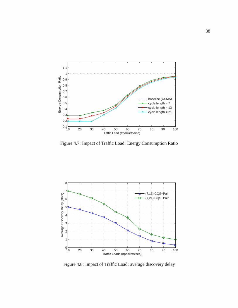
38

10 20 30 40 50 60 70 80 90 1000.1

0.2

0.3

0.4

0.5

0.6

0.7

0.8

0.9

1

1.1

Taffic Load (#packets/sec)

Ene

rgy

Con

sum

ptio

n R

atio

baseline (CSMA)cycle length = 7cycle length = 13cycle length = 21

Figure 4.7: Impact of Traffic Load: Energy Consumption Ratio

10 20 30 40 50 60 70 80 90 1000

1

2

3

4

5

6

7

8

Traffic Loads (#packets/sec)

Ave

rage

Dis

cove

ry D

elay

(sl

ots)

(7,13) CQS−Pair(7,21) CQS−Pair

Figure 4.8: Impact of Traffic Load: average discovery delay

39

is because, the communication schedule of a node will have more active slots, when compared withits quorum-based wakeup schedule during high traffic load. With more slots staying awake, theaverage discovery delay between two neighboring nodes will be significantly reduced.

4.1.7 Conclusions

We presented a theoretical approach for heterogeneous asynchronous wakeup scheduling in WSNs.We first defined the h-QPS problem—i.e., given two cycle lengths n and m (n < m), how todesign a pair of heterogeneous quorum systems to guarantee that two adjacent nodes that selectheterogenous quorums from the pair as their wakeup schedules can hear each other at least once inevery m consecutive time slots. We proposed two designs for heterogeneous asynchronous wakeupscheduling: the cyclic quorum system pair (cqs-pair) and the grid quorum system pair (gqs-pair).We also presented a fast construction scheme to assemble a cqs-pair. In our construction scheme,we first quickly construct an (n, k, 1)-difference set and an (m, l, 1)-difference set. Based on twodifference sets A in (Zn, +) and B in (Zm, +), we can construct a cqs-pair (C(A, Zn), C(B, Zm))when A and B can form a (n, k, m, l)-difference pair.

The performance of a cqs-pair and a gqs-pair were analyzed in terms of average delay, quorumratio, and energy saving ratio. We show that the average delay between two nodes that wakeup viaheterogenous quorums from a cqs-pair is bounded between n−1

2and m−1

2, and the quorum ratios

of the two quorum systems in the pair are optimal, respectively, given their cycle lengths n and m.For a gqs-pair with

√n × √n grid and

√m × √m grid, the average discovery delay is bounded

within (n−1)(√

n+1)3√

n< E(Delay) < (m−1)(

√m+1)

3√

m, while the quorum ratios are 2

√n−1n

and 2√

m−1m

,respectively.

4.2 Asymmetric Quorum-based Wakeup Scheduling

4.2.1 Motivations

Even though some works introduce adaptive configuration mechanism, like B-MAC [13] and T-MAC [24], for dynamically changing duration of time slots, these solutions may suffer energywaste in neighbor discovery over unreliable environment with link or node failures. The reasonis as follows. When a node send out preamble to detect one neighbor in a time slot, it probablydoes not receive an ACK (i.e., to indicate the presence) message from the neighbor within thattime slot; but the node cannot distinguish two possible causes of not receiving ACK: it may bebecause the neighbor has longer time slot so that the neighbor is still sleeping, or because ofunreliable environment which leads to message loss. Since the probing node cannot distinguishthe two possible reasons, it has to continuously send out preamble to probe its neighbor, which willcause huge energy waste if it takes a long time to recover the failed links. If the probing nodes use

40

some back-off mechanisms (i.e., exponential back-off), the neighbor discovery latency cannot bebounded.

Motivated by supporting energy-efficient neighbor discovery over unreliable environment and bysupporting asymmetric energy saving in idle state, we present p-Grid, an asynchronous neighbordiscovery protocol for low duty-cycled WSNs. In p-Grid, each node listens the channel states onlyin the beginning of selected time slots in every n consecutive time slots. Here, n is the cycle lengthand the selected time slots are referred as to a quorum schedule. When a node wants to discoverits neighbor, it stays awake and sends out preambles to probe its neighbors in selected time slotswhich are also referred as to a quorum schedule. Our design guarantees that the quorum-basedprobing schedule of a node will intersect at least once with the listening schedules of its neighborswithin bounded time slots.

In p-Grid, the asymmetric energy saving ratio is achieved by adopting asymmetric quorum-basedprobing scheduling and listening scheduling via grid quorum group design. By theoretical analysis,we show that p-Grid achieves flexibility for run-time configuration by selecting different quorumsfor listening and neighbor probing. It is also shown that p-Grid wastes less energy for detect-ing neighbors over unreliable environment, and can guarantee neighbor discovery within boundedlatency once the failed links are recovered.

The main objective in designing p-Grid is to support flexible run-time configuration of idle en-ergy saving ratio and to achieve energy efficiency for neighbor discovery over unreliable environ-ment. In addition, the protocol should be asynchronous for easy implementation and be easilyintegrated into existed MAC protocols or routing protocols. The following problems are involvedin our design: (1) how to designs an energy-efficient listening schedule and node probing sched-ule, rather than a simple periodic listening and probing as that in B-MAC or X-MAC; and (2) howto guarantee bounded neighbor discovery latency with non-periodic schedules; and (3) what is anenergy-efficient back-off mechanism in case of node failure over unreliable environment?

4.2.2 Protocol Design of p-Grid

4.2.2.1 Overview

The design of p-Grid is based on properties of quorum groups. A quorum group contains two typesof quorums: read quorum and write quorum which satisfy write∩write �= ∅ and read∩write �= ∅.There are two operations modes for each node in our design: listening mode and probing mode.In listening mode, a node checks the gain level of its channels to detect whether there is a messagecoming, in the beginning of selected time slots. In probing mode, a node will stay awake and sendsout short strobe preambles which is referred as to DISC messages in selected time slots. Every nodestay in listening mode in idle state. For neighbor discovery, the probing node simply switches fromlistening mode to probing mode, and then sends out preambles to probe its neighbors. When theneighbors detect the preambles, they will feedback REPLY messages to indicate their presence.

41

In p-Grid, the listening schedules of nodes in listening mode are complying with a read quorum.The probing schedules of nodes in probing mode are based on a write quorum. Since read ∩write �= ∅, a node in probing mode can definitely discover its neighbors in listening mode.

In order to achieve flexibility in run-time configuration of duty cycle, a node only needs to selecta schedule with different size, rather than changing the duration of each time slot. The boundedlatency is achieved by non-empty intersection property among read quorums and write quorumswithin one cycle of the quorum group. We will also show that our quorum-based schedules can actas good back-off schemes over unreliable environment.

4.2.2.2 Listening Mode and Probing Mode

We introduce the operations of nodes in listening mode and probing mode. The operations havesome similarities with previous duty-cycled asynchronous MAC protocols, like B-MAC [13] orX-MAC [27].

In our design, for nodes in listening mode, they check the channel states in the beginning of timeslots which are selected as read quorum that is defined in Definition 13. Let Rj denote the readquorum which contains the j th column of entries in the n × n array. A node checks the channelstate by dual preamble sampling in two separate periods P1 and P2 in each slot of Rj. Figure 4.9(a)shows an example. Here, the channel state is checked in the beginning of blue colored slots. Ifthe gain of the channel is less than a threshold, the node returns to sleep state after checking. Wechoose the dual preamble sampling in order to further reduce the awake time in listening mode.

Figure 4.9: Two operation modes and neighbor discovery procedure in p-Grid

In the probing mode, a node sends out a series of short strobe preambles in time slots which are

42

selected as write quorum that is defined in Definition 14. We denote the short preamble messageas DISC. Let Wj,i denote the write quorum which contains the j th column of entries and the ith

row of entries in the n× n array. Figure 4.9(b) shows an example for probing mode.

The neighbor discovery procedure, as shown in Figure 4.9(c), is as follows. A neighbor nodechecks its channel states during P1 and P2. If the channel is not free during P1, the neighbor nodeenters the sleep mode for a period of time and proceeds to receive DISC messages. The period P1

is necessary only when the channel is found to be free during P1. After receiving a DISC message,the node will immediately feedback an acknowledgement message, referred as to REPLY message,to the probing node, and will keep awake for one slot to receive any possible following messages.Otherwise, the neighbor node will keep staying in listening mode.

At the probing node side, if the probing node does not receive a REPLY message after sending aDISC message, it will continue to send out DISC messages until the current time slot expires. Theprobing node will continue to send out DISC messages in the next slot of Wj,i. If the incomingtime slot is not in Wj,i, the probing node will stay in the SLEEP state until the arrival of a next slotbelonging to Wj,i.

We formally define read quorum and write quorum as follows. Suppose the quorum group has an× n grid. We arrange n× n consecutive time slots into a n× n array.

Definition 13 [Read quorum] In a n×n array, we define the read quorum as a set containing anycolumn of time slots in the grid. If the read quorum contains the j th column of slots, we denote itas Qr

j .

Definition 14 [Write quorum] In a n × n array of consecutive time slots, we define the writequorum as a set containing any row of time slots in the grid. If the write quorum contains the i th

row of slots, we denote it as Qwi .

Definition 15 [Grid quorum group] In the n × n array, we define the grid quorum group as theset of all read quorums and write quorums.

As to the value of Rj and Wj,i, they can be selected randomly from a grid quorum group. We willshow the nonempty intersection property between an arbitrary read quorum and a write quorumin next section. In addition, there is difference between the grid quorum group and grid quorumsystems. In grid quorum groups, it is not necessary for two read quorums or two write quorumsto intersect with each other. But in grid quorum system, any two quorums have a non-emptyintersection.

4.2.2.3 Neighbor Discovery for Symmetric Groups

We first show the non-empty intersection property between read quorums and write quorums whichbelongs to same grid quorum groups. Such intersection property is the foundation for the neighbor

43

discovery within bounded latency.

Theorem 11 With one grid quorum group, a probing node equipped with a write quorum as itsprobing schedule must discover its neighbors equipped with a read quorum as listening schedulesby at least once, regardless of clock drift.

We omit the proof for Theorem 11. The formal proof is similar as the proof for asynchronousintersection property in [30]. An intuitive example is given in Figure 2. Two nodes adopt a 3× 3grid quorum group. The probing mode selects a write quorum containing the 2nd column plus the1st row in the grid. The listening mode selects a read quorum containing the 3rd column in thegrid. Regardless of clock drift, they have at least one overlapped slot within 3× 3 slots. With thehelp of preamble at probing node side and channel state checking at neighbor side, the probingnode can detect the neighbor node in its 2nd, 5th and 8th time slot.

Corollary 4 Two write quorums in a quorum group must have at least one intersection.

In order to reduce the discovery latency, it is better to select a write quorum which contains thefirst row of the grid so that the intersection will happen within the first n slots. We denote suchwrite quorum as Wj,1 where j ∈ [1..n].

In the procedure for neighbor discovery, the key step is quorum switch. A probing node has to firstswitch its listening schedule from a read quorum to a write quorum. The reason for doing quorumswitch is that two read quorum cannot guarantee non-empty intersection. Let the read quorum beRj and the write quorum be Wj′ ,1. After switching, although there is an increase in the quorumsize for write quorum, we have Rj ∩Wj′ ,1 �= ∅ within n2 time slots.

4.2.2.4 Neighbor Discovery for Asymmetric Groups

In order to satisfy different energy saving requirements for heterogenous nodes, it is desirable thattwo nodes adopt asymmetric listening scheduling patterns. For example, the listening schedule ofthe cluster head which has more power supply may use quorums from 3× 3 grid quorum groups,while the schedule for cluster members with less power resource uses quorums from 5 × 5 gridquorum groups. In this section, we present the neighbor discovery scheme in such scenario.

It is difficult to guarantee the non-empty intersection property between read quorums and writequorums from two arbitrary grid quorum groups. However, if we choose prime-grid quorum groupswhich are defined as follows, the nonempty intersection property can be satisfied.

Definition 16 In the grid quorum group with n×n time slots, if n is a prime, we define the quorumgroup as prime-grid quorum group.

44

Figure 4.10: Intersection between a write quorum and a read quorum from two prime-grid quorumgroups: the write quorum A from the grid quorum group Q3×3, and the read quorum B from thegrid quorum group Q5×5. A2

⋂B �= ∅

Definition 17 (p-extension). Given two positive integers n and p, for a set A = {ai|1 ≤ i ≤k, ai ∈ Zn}, the p-extension of A is defined as Ap = {ai+j∗n|1 ≤ i ≤ k, 0 ≤ j ≤ p−1, ai ∈ Zn}.

Example: Let A = {1, 2, 3, 4} in (Z16, +). Now, A2 = {1, 2, 3, 4, 17, 18, 19, 20} in (Z32, +).

Theorem 12 Consider two different prime-grid quorum groupsQA with n×n array andQB withm × m array. Suppose n < m and p = �m

n. The p-extension of a read quorum A ∈ QA must

have at least one intersection with a read quorum B fromQB , or Ap ∩ B �= ∅.

Proof 6 Let Ap = {a1, a2, · · · , an|ai < pn2}. All elements in A satisfy ai ≡ ra(mod n), where ra

is the residue and ra < n.

Let B = {b1, b2, · · · , bm}. All elements in B satisfy bi ≡ rb(mod m), where rb is the residue andrb < m.

Since n and m are prime numbers, according to the Chinese Remainder Theorem, there must bean integer I that satisfies I ≡ ra(mod n) ≡ rb(mod m) and I ≤ n ×m < m2. This means thatthere is an intersection between Ap and B.

Lemma 3 (small write to big read) Consider two prime-grid quorum groupsQA with n×n arrayandQB with m×m array. Suppose n < m. The p-extension (p = �m/n) of a write quorum Wj,i

fromQA must have at least one intersection with a read quorum Rj′ fromQB , or (Wj,i)p∩Bj′ �= ∅.

Proof 7 Let the read quorum consisting of the j th column of slots inQA be denoted as RAj. Since(RAj)

p ⊂ (Wj,i)p and (RAj)

p ∩Rj′ �= ∅, based on Theorem 12, we have (Wj,i)p ∩Rj′ �= ∅.

45

An illustration of Lemma 3 is given in Figure 4.10. There are two grid quorum groups in Fig-ure 4.10, one with a 3×3 grid and another one with a 5×5 grid. We can see that the write quorumA in the smaller group will intersect with the read quorum B of the bigger group at three timeslots.

Lemma 4 (big write to small read) Consider two prime-grid quorum groupsQA with n×n arrayand QB with m ×m array. Suppose n < m and p = �m

n. A write quorum Wj,i from QB must

have at least two intersections with the p-extension of a read quorum Rj′ fromQA.

We omit the proof for Lemma 4 since it is intuitive.

Theorem 13 Given two adjacent nodes and two prime-grid quorum groups Qn×n and Qm×m, ifone node adopts a read quorum from Qnn and the other node adopts a write quorum fromQm×m,the two nodes can discover each other within max{n2, m2} time slots, by operating in listeningmode and probing mode separately.

Proof 8 Assume that the read quorum is R fromQn×n and the write quorum is W fromQm×m.

Without loss of generality, assume that the read quorum is Qr fromQn×n and the write quorum isQw fromQm×m.

Case 1: n = m. R and W must have an intersection within n2 slots, according to Theorem 11.

Case 2: n < m. p = �m/n. Based on Lemma 4, Rp and W must have at least two intersectionswithin m2 slots.

Case 3: n > m. p = �n/m. Based on Lemma 4, Rp and W must have at least one intersectionwithin n2 slots.

Since there must be an overlapped slot between R and W , the nodes will discover each other withthe help of dual preamble sampling and shorted strobed RTS.

4.2.2.5 Backoff Mechanism in Unreliable Environment

With asymmetric design, when a node does not receive REPLY message after sending out DISCmessage, it is probably because the neighbor choose a bigger quorum group, or because of linkfailures. But the probing node cannot distinguish the two possible reasons.

By nature, our design can provide an energy efficient back-off mechanism to avoid periodic retriesafter not receiving a REPLY message. In p-Grid, the node who wants to discovery others willgradually enlarge the cycle length of the grid quorum group for its probing scheduling when thereis no REPLY messages received in one quorum cycle, until timeout. The value of timeout is setin specific application requirement, e.g, in a network with node mobility, the value can be smallercompared to the value in a static network.

46

Since we adopt prime-grid quorum group design, the back-off mechanism is operated as follows: anode in probing mode chooses a quorum group sized with n2

1 , if the node does not receive REPLYmessage after some cycles (i.e. ≥ 3, it is dependent on user configuration), the node chooses abigger quorum group sized with n2

2 , if the node still does not receive REPLY message within n22

time slots, the node chooses a bigger group sized with n23. The node will continue to increase the

size of next quorum group, until timeout. Suppose the last quorum group before timeout is sizedby np × np, the selecting sequence satisfies,

n1 < n2 < · · · < np

whether n1, n2, · · · , np are primes.

The rationale for the backoff mechanism is straightforward. With the increasing of quorum groupcycle, at some time, the cycle n2

k (1 ≤ k ≤ p) will be equal to or bigger than the cycle of neighbors,which can meet the non-empty intersection property within one cycle, according to Lemma 4.

As we will show in Section 4.2.2.2, it is more energy efficient with larger quorum cycles. There-fore, we can achieve energy efficiency in unreliable environment by enlarging the size of selectedgrid quorum group, but meanwhile guarantee the neighbor discovery.

4.2.3 Performance Analysis

In this section, we show the energy efficiency of p-Grid in unreliable environment and its flexibilityin supporting heterogenous energy saving ratio.

For the purpose of easy presentation, we denote Ti as the length of one time slot, Tawake as thetotal time duration for channel sampling(s) and Ts as the time duration for single channel sampling(Tawake = 2Ts for dual preamble sampling). Suppose there are two prime grid quorum groups:Qn×n and Qm×m(n < m, n and m are primes).

The typical value for Ti in our design is set to 50ms. We set the default duration for preamblesampling (Ts) as 3 milliseconds when a node performs a sequence of operations to startup theradio, and set the radio in the RX mode, which is default to the setting in [13]. Thus the totalduration for the dual preamble sampling is 6 milliseconds.

4.2.3.1 Flexibility of Configuration

Suppose the grid quorum group is Qn×n whose time axes is organized into consecutive slots witha n× n array.

We define the idle energy consumption ratio as the total awake time to the whole operation time fora node. Suppose the duty cycle in a single time slot is α = Tawake

Ti, where Tawake is the duration for

channel sampling. In our dual preamble sampling scheme, Tawake = 2Ts. The quorum ratio, whichis the proportion of the size of a quorum in a whole quorum group cycle, is 1

nfor read quorums.

47

Thus, the overall idle energy consumption ratio for read/write quorums in Qn×n in idle state is:φ = 1

n· α.

The overall idle energy consumption ratio for write quorums inQn×n in idle state is:

φ =2n− 1

n2· α (4.1)

To support different idle energy saving requirement, a node only needs to adjust its quorum ratio,1n

for read/write quorums and 2n−1n2 for write quorums. This can be done by selecting different

grid quorum group in a node. The convenience of run-time configuration stems from no changesfor duty cycle in a singe time slot. The run-time configuration can be implemented in applicationlayer.

4.2.3.2 Energy Efficiency in Unreliable Environment

For XMAC-ALPL, suppose that the cluster-head adopts a checking interval with duration of Lc

and the cluster members adopt a checking interval with duration of Lm (Lc ≤ Lm).

In p-Grid, suppose that the cluster-head adopts a quorum group of Qn×n and the cluster membersadopt a Qm×m.

Theorem 14 In reliable environment with no link failure, the worst case energy consumption ofp-Grid for neighbor discovery is same as that of XMAC-ALPL, with respect to same idle energyconsumption ratio.

Proof 9 Suppose the duration of channel checking in both p-Grid and XMAC-ALPL is Tawake. Theidle energy consumption ratio of XMAC-ALPL for the cluster-head is Tawake/Li. The idle energyconsumption ratio of p-Grid is Tawake

Ti∗n . If the two mechanisms have same idle energy consumptionratio, we have Lc = Ti ∗ n. Regarding cluster members, similarly, we have Lm = Ti ∗m.

Case 1: The cluster member is the sender. For neighbor discovery, the worst cast awake time inXMAC-ALPL will be Lc since the cluster member will definitely discover the cluster head after Lc

once it begins to send out preamble.

The worst case awake slots for the cluster members in p-Grid will be n slots before discovering thereceiver. The awake time will be Ti ∗ n. Since Lc = Ti ∗ n, the worst case energy consumption ofp-Grid for per neighbor discovery is same as that of XMAC-ALPL.

Case 2: The cluster head is the sender. We can prove the theorem similarly as that in case 1.

Theorem 15 In unreliable environment with link failures, the worst case energy consumption ofp-Grid for neighbor discovery is better than that of XMAC-ALPL, with respect to same idle energyconsumption ratio.

48

Proof 10 Case 1: The cluster member is the sender. In unreliable environment, the senders withXMAC-ALPL mechanism have to send out preamble continually. Thus for neighbor discovery, theworst cast awake time of the sender will be k ∗ Lc where the kink will recover in the kth slots afterthe initial link failure.

As to p-Grid, the sender will discover the receiver within � k∗Lc

m∗n∗Ti quorum slots. The awake time

is � k∗Lc

m∗n∗Ti∗Ti. If m > 1 and n > 1, we have � k∗Lc

m∗n∗Ti∗Ti ≤ ( k∗Lc

m∗n∗Ti+1)∗Ti = ( k

m∗n + 1n)∗Lc ≤

k ∗ Lc.

Case 2: The cluster member is the sender. We can make similar proof.

Thus, p-Grid is energy-efficient than XMAC-ALPL in unreliable environment. In reliable situa-tion, they can achieve same performance regarding energy efficiency as claimed in Theorem 14.

4.2.3.3 Bounded Neighbor Discovery Latency

Discovery latency of homogenous case: We define the discovery latency as the time between thedata arrival and the discovery of the adjacent receiver (i.e., receiving the CTS message from thereceiver). Note that this metric does not include the time for delivering a message.

Theorem 16 The average discovery latency between two nodes that use a read quorum and awrite quorum, respectively, from the same grid quorum group Qn×n as their LPL schedules isD = n

2· Ti.

Proof 11 The latency can be divided into two parts: 1) the latency for finding the first intersection,denoted as D1; and 2) the latency to hear from the receiver within the intersected slot, denoted asD2.

For the first part, suppose the write quorum is Qwj,1 and the read quorum is Qr

j′ . The probability of

Qrj′ overlapping with Qw

j,1 in the kth (1 ≤ k ≤ n) slot of Qwj,1 is 1/n, with corresponding latency

(k − 1) · Ti. Thus,

D1 =1

n

n∑k=1

(k − 1) · Ti =n− 1

2Ti (4.2)

For the second part, with clock drift, the average latency to hear from the first CTS message fromthe receiver is D2 = Ti/2. Summing up the two parts, D = D1 + D2 = n

2· Ti.

Discovery latency of heterogenous case: Suppose two prime-grid quorum groupsQn×n andQm×m.Without loss of generality, let n < m.

49

…

… …

… …

… … … … … …

……

……

n n m-n

m

… …

… … … … … …

……

……

n m-n

m

A B1 B2

Figure 4.11: An example of the intersection between a big read quorum and a small write quorum.Case 1: intersection within the first n slots of A; case 2: intersection beyond the first n slots of A.

Theorem 17 (big write to small read) Suppose Qrj ⊂ Qn×n and Qw

j′,1⊂ Qm×m (n < m). The

average discovery latency between two nodes that adopt Qrj and Qw

j′,1

for their LPL schedules,respectively, is n

2· Ti.

The proof of Theorem 17 is default to that for Theorem 16.

Theorem 18 (small write to big read) Suppose Qwj′ ,1 ∈ Qn×n and Qr

j ∈ Qm×m (n < m). Theaverage discovery latency between two nodes that adopt Qr

j and Qwj′ ,1, respectively, is:

D =n(m− n + 1)

2· Ti (4.3)

Proof 12 Similar to the proof of Theorem 16, the latency can be separated into two parts. We firstderive the value of the latency part for reaching the first intersection.

As shown in Figure 4.11, suppose the time difference between two nodes is Δ. Then 0 ≤ Δ < nTi

due to the rotation property of the grid quorum group. We consider two cases to derive this latencypart:

Case 1: 1 ≤ (j+ ΔTi

) mod n ≤ n for Qrj ⊂ Qm×m, i.e., the quorum B1 in Figure 4.3. Suppose Qr

j

intersects with Qwj′ ,1 in the kth (1 ≤ k ≤ n) slot of Qw

j′ ,1. The corresponding latency is (k − 1) · Ti

and the probability is 1/m. Thus, the average latency for this case is:

Dcase1 =1

m

n∑k=1

(k − 1)Ti =n(n− 1)

2m· Ti

Case 2: n < (j + ΔTi

) mod n ≤ m for Qrj ⊂ Qm×m, i.e., the quorum B2 in Figure 4.3. For this

case, Qrj will not overlap with Qw

j′,1

within the 1st row ofQn×n.

The intersection will happen in one slot of the read quorum Qrj′ ⊂ Qn×n, except for the first

element of Qrj′ .

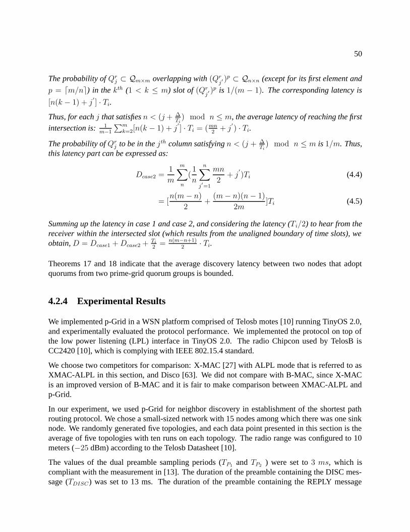
50

The probability of Qrj ⊂ Qm×m overlapping with (Qr

j′ )p ⊂ Qn×n (except for its first element and

p = �m/n) in the kth (1 < k ≤ m) slot of (Qrj′ )p is 1/(m − 1). The corresponding latency is

[n(k − 1) + j′] · Ti.

Thus, for each j that satisfies n < (j + ΔTi

) mod n ≤ m, the average latency of reaching the first

intersection is: 1m−1

∑mk=2[n(k − 1) + j

′] · Ti = (mn

2+ j

′) · Ti.

The probability of Qrj to be in the jth column satisfying n < (j + Δ

Ti) mod n ≤ m is 1/m. Thus,

this latency part can be expressed as:

Dcase2 =1

m

m∑n

(1

n

n∑

j′=1

mn

2+ j

′)Ti (4.4)

= [n(m− n)

2+

(m− n)(n− 1)

2m]Ti (4.5)

Summing up the latency in case 1 and case 2, and considering the latency (Ti/2) to hear from thereceiver within the intersected slot (which results from the unaligned boundary of time slots), weobtain, D = Dcase1 + Dcase2 + Ti

2= n(m−n+1)

2· Ti.

Theorems 17 and 18 indicate that the average discovery latency between two nodes that adoptquorums from two prime-grid quorum groups is bounded.

4.2.4 Experimental Results

We implemented p-Grid in a WSN platform comprised of Telosb motes [10] running TinyOS 2.0,and experimentally evaluated the protocol performance. We implemented the protocol on top ofthe low power listening (LPL) interface in TinyOS 2.0. The radio Chipcon used by TelosB isCC2420 [10], which is complying with IEEE 802.15.4 standard.

We choose two competitors for comparison: X-MAC [27] with ALPL mode that is referred to asXMAC-ALPL in this section, and Disco [63]. We did not compare with B-MAC, since X-MACis an improved version of B-MAC and it is fair to make comparison between XMAC-ALPL andp-Grid.

In our experiment, we used p-Grid for neighbor discovery in establishment of the shortest pathrouting protocol. We chose a small-sized network with 15 nodes among which there was one sinknode. We randomly generated five topologies, and each data point presented in this section is theaverage of five topologies with ten runs on each topology. The radio range was configured to 10meters (−25 dBm) according to the Telosb Datasheet [10].

The values of the dual preamble sampling periods (TP1 and TP2 ) were set to 3 ms, which iscompliant with the measurement in [13]. The duration of the preamble containing the DISC mes-sage (TDISC) was set to 13 ms. The duration of the preamble containing the REPLY message

51

(TREPLY ) was set to 7 ms. Besides, we set other parameters in our experimental study as follows:DISC/REPLY message size was set to 128 bytes, and data packet size was 512 bytes.

Three important metrics were measured in our experimental study: (1) energy consumption ratio;and; (2) neighbor discovery latency; and (3) neighbor discovery ratio.

4.2.4.1 Energy Consumption Ratio

We first demonstrated the energy efficiency of p-Grid. For the purpose of easy measurement, wedid not measure the actual energy consumed directly, but the average awake time for all nodes. Inour experiment, a node went to listening mode immediately after completing neighbor discovery.

We set the length of one time slot as 50ms in p-Grid. We adopted the prime-grid quorum groupQ3×3 for read and write quorums, which has an energy consumption ratio of 1

3· 2∗3

50= 4% in

the idle state. To make a fair comparison, we also ameliorated XMAC-ALPL with dual-preamblemechanism by setting the length of one slot as 150ms (energy consumption ratio= 6

150= 4% in idle

state). For the sake of heterogenous configuration, we chose the prime-grid quorum group Q5×5

for some nodes, which has an energy consumption ratio of 15· 2∗3

50= 2.4% in the idle state. For the

XMAC-ALPL parameter setting of these nodes, we set the length of time slot as 250ms (energyconsumption ratio= 6

250= 2.4% in idle state).

For the Disco protocol, we used the (37, 43) balanced primes and symmetric pairs ( 123

+ 143

= 6.6%for cluster heads and cluster members, so that the total duty cycle was almost same as that in p-Gridand X-MAC. The slot length was set to 10ms.

Regarding the Disco protocol, we selected the (23, 43) balanced primes and symmetric pairs ( 123

+143

= 6.6%) for heterogenous nodes, respectively. Thus, the energy consumption ratio in idle statewas almost the same as that in p-Grid and XMAC-ALPL. The slot length of Disco was set to 10ms.

We varied the neighbor discovery frequency from once per second to 5 times per second, we firstmeasured the average awake time over reliable environment. As shown in Figure 5, the averageawake time at probing node side increased with larger neighbor discovery frequency in p-Gridand XMAC-ALPL. The average awake time of Disco increased slightly since it was mainly deter-mined by the prime selection without depending on specific neighbor discovery frequency. It isalso shown that p-Grid consumed almost the same energy (i.e., awake time) as that for XMAC-ALPL, which coincides with our analysis in Section 4.2.3. Note that the awake time of p-Grid orXMAC-ALPL is higher than that of Disco in Figure 4.12. However, Disco achieves lower energyconsumption at the cost of longer neighbor discovery latency and lower discovery ratio which willbe shown later.

As to the performance comparison for unreliable environment, we set the node failure probabilityas 0.3 for all nodes in all mechanisms. As shown in Figure 4.12, at the probing node side, all nodeswith p-Grid mechanism always took less awake time for discovering neighbors comparing withthat in XMAC-ALPL, since all nodes with p-Grid took less time for sending preamble in order

52

to find out the receiver in case of link failures. At the neighbor sides, the awake time of p-Grid,XMAC-ALPL and Disco were almost identical.

Figure 4.12: Energy Consumptions: reliable environment (left); unreliable environment with nodefailure probability being 0.3(right)

4.2.4.2 Neighbor Discovery Latency

We define neighbor discovery latency as the time delay between sending out DISC messages andreceiving the REPLY message from a neighbor. The purpose of the evaluation in this Section wasto verify the bounded neighbor discovery latency of p-Grid as claimed in Theorems 17and 18.

The protocol configurations for p-Grid, XMAC-ALPL, and Disco were the same as that in Sec-tion 4.2.4.1 to ensure that they had almost the same energy consumption ratio in the idle listeningmode.

PrimeGrid X−MAC Disco0

200400600800

16001800200022002400

Ave

rage

Dis

cove

ry L

aten

cy (

ms)

Figure 4.13: One-hop discovery latency between a read quorum and write quorum from the samegrid quorum group Q5×5

In Figure 4.13, we observe that p-Grid achieves slightly low latency than X-MAC. Although p-Grid may need more time slots for a node to intersect with its neighbor’s schedule, p-Grid usesshorter time slots (e.g., 50ms), which can still guarantee lower discovery latencies. For Disco,

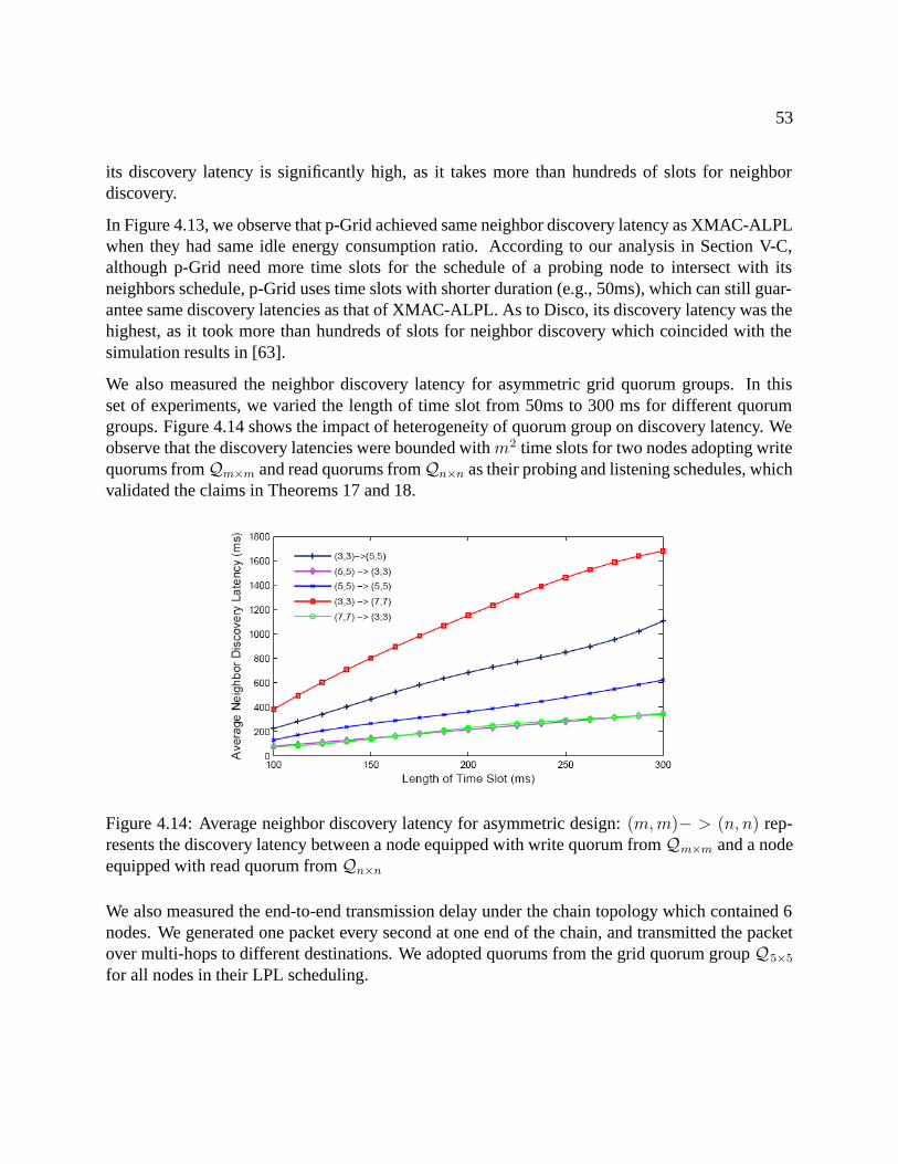
53

its discovery latency is significantly high, as it takes more than hundreds of slots for neighbordiscovery.

In Figure 4.13, we observe that p-Grid achieved same neighbor discovery latency as XMAC-ALPLwhen they had same idle energy consumption ratio. According to our analysis in Section V-C,although p-Grid need more time slots for the schedule of a probing node to intersect with itsneighbors schedule, p-Grid uses time slots with shorter duration (e.g., 50ms), which can still guar-antee same discovery latencies as that of XMAC-ALPL. As to Disco, its discovery latency was thehighest, as it took more than hundreds of slots for neighbor discovery which coincided with thesimulation results in [63].

We also measured the neighbor discovery latency for asymmetric grid quorum groups. In thisset of experiments, we varied the length of time slot from 50ms to 300 ms for different quorumgroups. Figure 4.14 shows the impact of heterogeneity of quorum group on discovery latency. Weobserve that the discovery latencies were bounded with m2 time slots for two nodes adopting writequorums fromQm×m and read quorums fromQn×n as their probing and listening schedules, whichvalidated the claims in Theorems 17 and 18.

Figure 4.14: Average neighbor discovery latency for asymmetric design: (m, m)− > (n, n) rep-resents the discovery latency between a node equipped with write quorum fromQm×m and a nodeequipped with read quorum from Qn×n

We also measured the end-to-end transmission delay under the chain topology which contained 6nodes. We generated one packet every second at one end of the chain, and transmitted the packetover multi-hops to different destinations. We adopted quorums from the grid quorum group Q5×5

for all nodes in their LPL scheduling.

54

4.2.4.3 Neighbor Discovery Ratio

We define neighbor discovery ratio as the times successfully get a REPLY message in one cy-cle divided by the total times of neighbor probing by a node. We varied the neighbor discoveryfrequency from once per second to at most eight times per second.

(a) node failure probability = 0.1

(b) varying failure probability for p-Grid

Figure 4.15: Neighbor discovery ratio: a). different protocols; b). different failure ratios

We first fixed the node failure probability with 0.1 for all nodes and compared the performances.From Figure 4.15(a), we observe that p-Grid and XMAC-ALPL achieved higher delivery ratio thanDISCO since both of them use the acknowledgement mechanism - i.e., the probing node sendingthe preamble and the neighbor acknowledging the receipt of the preamble (DISC message). Incontrast, Disco achieved a lower delivery ratio because the long discovery latency of Disco resultedin the dropping of packets in the local memory buffer, especially for high neighbor discoveryfrequency

We also varied the node failure probability from 0.1 to 0.5 in order to evaluate the reliability of

55

p-Grid. In Figure 4.15(b), it is shown that the neighbor discovery ratio decreased with bigger nodefailure probability and that the ratio decreased with higher neighbor discovery frequency, whichindicated that p-Grid cannot work well in highly unreliable environment.

4.2.5 Conclusions and Discussions

We presented a flexible solution, p-Grid, for neighbor discovery service in low duty-cycled WSNs.The motivation was to provide an energy-efficient, run-time configurable, asynchronous neighbordiscovery mechanism for WSNs over unreliable environment. p-Grid is easy to implement: in idlestate, nodes select a read quorum from a prime-grid quorum group as their low power listeningschedules. For neighbor discovery, a node switches from listening mode to probing mode byselecting a write quorum from a prime-grid quorum group as its probing schedules, and sends outDISC messages in the time slots selected as write quorum. Armed with the prime-grid quorumgroup design, we show that there must be at least one overlapped slot in which both the probingnode and its neighbors in listening mode are awake simultaneously.

It is possible that in p-Grid two or more REPLY messages collide at the probing node side, resultingin neighbor discovery failure. To address the collision, two strategies can be applied. One is thateach node shifts its schedule by random time slots 8 after a time period so that nodes will not listenat the same time moment. Another one is by mutual neighbor discovery. A neighbor node alsotries to detect the previous probing node and hence informs its presence to the previous probingnode.

The design of p-Grid belongs to asynchronous neighbor discovery mechanisms so that time-synchronization is not necessary. Thus, it has the advantages of scalability. p-Grid can be inte-grated into existing MAC protocols or routing protocols to provide neighbor discovery service.We can also apply p- Grid for providing fault-tolerance functionality in WSNs. With some ex-tensions, p-Grid can be adapted as a MAC protocol for delay-tolerant data communications inscenario where realtime data delivery is not mandatory.

In two-tiered WSNs, to meet heterogenous idle energy saving requirements, the cluster head shoulduse a prime-grid quorum group with smaller size, and the cluster members should adopt a prime-grid quorum group with bigger size, because the discovery latency between quorums with smallerquorum size is shorter as shown in Section V. Thus, with a smaller grid quorum group for clusterheads, which may act as virtual routers in WSNs, the end-to-end transmission latency will bereduced resulting from shorter neighbor discovery latency. To compensate for imbalances in energyconsumption for different nodes, the rotation mechanism of [94] can be applied by rotating theroles of all nodes.

Thus, p-Grid achieves performance trade-off between energy saving and neighbor discovery la-tency, which indicates lower energy consumption ratio with higher latency, and higher energyconsumption ration with lower latency.

We envision several future directions for this work. One direction is to consider other quorum

56

systems, e.g., cyclic quorum systems, for the purpose of further reducing the discovery latency.Another direction is to combine the p-Grid protocol with a routing protocol to make an optimalcross-layer design for end-to-end data transmission.

Chapter 5

Routing over Heterogenous WakeupScheduling

5.1 Motivations

Multihop data routing over WSNs has attracted extensive attention in the recent years. Since thereis no fixed infrastructure in sensor networks, the routing problem is different from the one in tra-ditional wired networks or the Internet. Some routing protocols [91, 95] over WSNs presented inthe literature are extended from the related approaches over wired/wireless ad-hoc networks. Theyusually find a path with the minimum hop count to the destination, which is based on the assump-tion that the link cost (or one-hop transmission latency) is relatively static for all wired/wirelesslinks. However, for duty-cycled WSNs [13, 15, 27], that assumption may not be valid any more.

Duty-cycled WSNs include sleep-wakeup mechanisms, which can violate the assumption of staticlink costs. Currently, many MAC protocols support WSNs operating with low duty cycle, e.g.,B-MAC [13], X-MAC [27]. In such protocols, sensor nodes operate in low power listening (orLPL) mode. In the LPL mode, a node periodically switches between the active and sleep states.The period for one active/sleep switching is called the LPL checking interval, which can be iden-tical, or can be adaptively varied for different nodes, referred to as ALPL [18]. The duty-cycledmechanism have been shown to achieve excellent idle energy savings, scalability, and easiness inimplementation. However, they suffer from time-varying neighbor discovery latencies, which isalso pointed out by Ye et.al. [39]. As shown in Figure 5.1, the neighbor discovery latency betweentwo neighbors is varying with different departure times. Even with synchronized duty-cycling, theneighbor discovery latency is varying at different time moments due to adaptive duty cycle settingas shown in Figure 5.1.

To formally define the problem, we first define the link cost as the time delay between data dis-patching time at a sender and the data arrival time at the receiver. The link cost is time-varying inadaptively duty-cycled WSNs due to varying neighbor discovery latency, even though the physical

57

58

propagation condition does not change with time. The dispatching time means the time momentwhen the data is ready for transmission at the sender side. Thus, this raises a non-trivial problem:with time-varying link costs, how to find optimal paths with least nodes-to-sink latency for allnodes at all discrete dispatching time moments?

A similar problem has been modeled by previous works as the time-dependent shortest path prob-lem (or TDSP) [50, 73] in the field of traffic networks [49], time-dependent graphs [74], and GPSnavigation [75]. The general time-dependent shortest path problem is at least NP-Hard since itmay be used to solve a variety of NP-Hard optimization problems such as the knapsack problem.However, depending on how one defines the problem, it may not be in NP, since its output isnot polynomially bounded. Moreover, there are even continuous-time instances in which shortestpaths consist of an infinite sequence of arcs as shown by Orda and Rom [96]. In the disseration,we study a special case where the networks are known as FIFO networks, in which commoditiestravel along links in a First-In-First-Out manner. Under the FIFO condition, the time-dependentshortest path problem is solvable in polynomial time.

The problem has also been studied with a distributed approach. For distributed solutions of theproblem, the only previous work [50] computes the shortest paths for a specific departure timein each execution. If the whole time period has M discrete intervals (M is ∞ for infinite timeintervals), we have to execute the algorithm in [50] M times, which is inefficient in terms ofmessage complexity and time complexity, given the limited power and radio resource in WSNs.Therefore, the first motivation of our work is to design a fast distributed algorithm for the problem,which can efficiently enumerate all optimal paths with least end-to-sink latency for infinite timeintervals.

The second motivation of our work is to propose an algorithm which can dynamically and distribu-tively maintain time-dependent least-latency paths. In WSNs, a node may update its duty-cycleconfiguration (e.g., based on its residual energy), or join or leave the network, thereby changingthe network topology. In such situations, the duty-cycle updating node or the joining/leaving nodemay change the cost of all the links with its neighbors, which means that a single node updatecan cause multiple link updates. Previous efforts on this problem [76, 77] are efficient in handlingsingle link updates. Applying such solutions for multiple link updates would imply that multipledistributed updates execute concurrently for a single node update, which is not efficient in termsof message and memory space complexities for resource-limited WSNs.

The third motivation of our work is to address practical implementation issues. One is to under-stand how to address the awareness of duty cycling of neighborhood. We discuss several under-lying mechanisms, such as B-MAC, S-MAC, and quorum-based wakeup scheduling, and proposea method for schedule awareness over them. Another is to understand how to simplify the vectorpresentation so that only smaller vector sizes are required, given the limited memory resource forembedded sensor nodes. We present a sub-optimal implementation, which achieves a trade-off be-tween latency and memory usage. Finally, we discuss the complexities of our algorithms in somespecial scenarios, like static link costs and multiple sink nodes.

In this part of research, we first propose a distributed algorithm to compute the time-dependent

59

paths with least-latency for all nodes in a duty-cycled WSN. The algorithm has low message andspace complexities. The algorithm is based on the observation that the time-varying link costfunction is periodic, and hence by derivation, the time-varying distance function for each node isalso periodic. We show that the link cost function satisfies the FIFO property [73]. Therefore,the time-dependent shortest path problem is not a NP-hard problem, and therefore is solvable inpolynomial time. We also propose distributed algorithms for maintaining the shortest paths. Theproposed algorithms re-compute the routing paths based on previous path information.

The message complexity of our algorithms is O(δ2) per node update, where δ is the number ofnodes that change either the distance or the parents in their shortest paths to the sink as a con-sequence of the corresponding nodes’ update. The algorithms’ space complexity is O(maxdeg),which is scalable for large-scaled networks. Finally, we propose a sub-optimal implementationwhich requires vectors with smaller sizes to represent link cost functions and the distance function.

The contributions of our works on this parts are as follows: 1. We model adaptively duty-cycledWSNs as time-dependent networks. We show that such networks satisfy the FIFO condition andthe triangular path condition; 2. We present distributed algorithms for finding the time-expandedshortest paths to the sink node for all nodes. When compared to the previous solution [50], ouralgorithms find the shortest paths in a single execution for infinite time intervals; 3. We present dis-tributed shortest path maintenance algorithms with low message complexity and space efficiency;and 4. We propose sub-optimal implementation with vector compression.

5.2 Problem Formulations

We model an adaptively duty-cycled WSN as a directed graph G = (V, E, C), with |V | nodes and|E| links. C = {τi,j(t)|(i, j) ∈ E} is a set of time-dependent link delays, i.e., τi,j(t) is a strictlypositive function of time defined for [0,∞), describing the delay of a message over link (i, j) attime t. Each node ni only knows the identity of the nodes in its neighbor set, defined as Ni.

We assume that time axes is arranged as consecutive short time slots. We denote the duration ofone time slot for node ni as Ti. It is possible that Ti �= Tj (ALPL) for two nodes ni and nj . Thetime expansion of each node ni is modeled as discrete and infinite, where Ti = {t0i , t1i , t2i , · · · , tMi },M is +∞, and tki −tk−1

i = Ti. We use the terms of checking interval and time slot interchangeably.

The wakeup schedule depends the underlying MAC protocols. We first assume a node can beoperated with LPL mode where a node wakes up at the beginning of a time slot to check thechannel state. If there is no activity, the node goes back to sleep, otherwise, it should stay awake.Then we relax the assumption and discuss how our works can be applied to other wakeup scheduleslike quorum schedules [1].

We consider the policy of no waiting at each node since the node-to-sink delay will not benefitfrom waiting. Thus, once the data arrives at an intermediate node, the node will try to dispatch thedata immediately. Dispatching times are not the same as the data departure times, as the data may

60

still be buffered in the sender’s memory. For simplicity in modeling and design, a node dispatchesthe received data at tki ∈ Ti.

A nonnegative travel time τi,j(tki ) is associated with each link (i, j) with the following meaning: If

tki is the data dispatching time from node ni along the link (i, j), then tki +τi,j(t

ki ) is the data arrival

time at node nj .

The general problem of determining the shortest paths with the least latency in time-dependentWSNs can be defined as follows: Find the least time paths from all nodes to the sink node ns

corresponding to the minimum achievable delay di, ∀ni ∈ V and ∀tki ∈ Ti, where

di(tki ) = min

nj∈Ni

{τi,j(tki ) + dj[t

ki + τi,j(t

ki )]} (5.1)

Equation 5.1 is an extension of Bellman’s equations [90] for the time-dependent network and isreferred to as TD-Bellman’s equation hereafter.

We assume that time slots in each node are numbered, and assume that the length of the datapackets is fixed or relatively small, which is valid for a WSN designed for a specific application.

We also assume that a message arrives correctly with finite time from a sender to a receiver, whichcan be achieved by any reliable MAC-layer transmission mechanism. The network is not assumedto be time-synchronized, and nodes do not synchronize their wakeup/sleep schedules. However,we assume the awareness of wakeup schedules of neighborhood. We further assume that all nodeshave the same time frequency, and their clocks drift at relatively slow speeds.

We do not explicitly consider radio interference in the problem modeling. We consume the inter-ference can be concealed by sleeping, RTS/CTS mechanism, and multiple radio or frequencies.

5.3 Modeling Adaptively Duty-cycled WSNs

In this section, we model adaptively duty-cycled WSNs as time-dependent networks. We showthat the link cost function is periodic and establish that the time-varying distance function is alsoperiodic. Having done so, we then implement TD-Bellman’s Equation by vector operations.

5.3.1 Link Cost Function

Without loss of generality, suppose there are two adjacent nodes ni and nj , where ni is the senderand nj is the receiver.

Suppose at time t0i , the neighbor discovery latency is Δt0ii,j. Then at time tk

i = t0i + k ∗ Ti, theneighbor discovery latency can be expressed as:

Δtkii,j = Tj − (k ∗ Ti −Δ

t0ii,j)mod Tj (5.2)

61

t0 ti

ni

nj

Ti

Tji,j i,jt0 t1

Figure 5.1: Varying neighbor discovery latency in heterogenous LPL mode

In an actual deployment, we can measure Δt0ii,j in the following way: at the beginning of the time

slot which starts at t0i , node ni sends out a preamble which contains the node ID of nj, and nj

immediately feeds-back an ACK containing the value of Tj once it receives the preamble. Afterreceiving the ACK by ni, the one-hop round trip delay from t0i to the time at which the ACK is

received is set to Δt0ii,j. Once we measured Δ

t0ii,j, Δ

tkii,j (k ≥ 0) can be computed by Equation 5.2.

For data transmission with fixed length data packets, we define the data propagation time as τdata.Now, for a directed link (i, j), we can set the link cost function as, for ∀tk

i ∈ Ti,

τi,j(tki ) = Tj − (k ∗ Ti −Δ

t0ii,j)mod Tj + τdata (5.3)

If τdata is relatively small when compared with Ti and Tj, we can set τdata = 0. This is espe-cially true for some WSN applications with small information reports, such as target tracking andenvironment monitoring.

Theorem 19 For every link (i, j), the time-varying link cost function is periodic. The minimumperiod for the function regarding k is,

P (τi,j) =LCM(Ti, Tj)

Ti(5.4)

where τi,j(tki )=τi,j(t

k+P (τi,j)i ) (k ≥ 0) and LCM is the least common multiple.

5.3.2 Distance to Sink

We refer to the node-to-sink delay as distance, for compatible representation with that in the staticBellman-Ford algorithm [90].

Consider node ni and its neighbor nj , where Ti �= Tj . For dispatching time t0i at ni, let us supposethat the data arriving time at nj is tj0j . Then, for the dispatching time tk

i at ni, with the same time

frequency for the two nodes, the corresponding time instant at nj is tj0j −Δt0ii,j +k∗Ti. Hence, based

on the neighbor discovery mechanism (i.e.,B-MAC [13] and X-MAC [27]), nj will be discovered

by ni at the time instant tj0j + �k∗Ti−Δ

t0ii,j

Tj ∗ Tj, with respect to nj’s time clock. Therefore, the

62

function of distance of ni to ns from the path through nj is:

di(tki ) = τi,j(t

ki ) + dj(t

k′+j0

j ) (5.5)

for ∀tki ∈ Ti, where k′= �(k ∗ Ti −Δ

t0ii,j)/Tj for tk

′j ∈ Tj, and j0 is the data arriving time slot at

nj with respect to dispatching time t0i .

Theorem 20 For a path ni → ni−1 · · · → n1 → ns, the distance function di(tki ),∀tki ∈ Ti, is a

periodic function, where the minimum period for the function regarding k is:

P (di) =LCM(T0, T1, · · · , Ti)

Ti

(5.6)

for di(tki ) = di(t

k+P (di)i ), where T0, T1, · · · , Ti are durations of the LPL checking intervals of nodes

ns, n1, · · · , ni, respectively.

Proof 13 The proof is by induction. For i = 1, d1(tk1) = τ1,s(t

k1) + ds(t

k′

1 ). Since ds ≡ 0,d1(t) = τ1,s(t

k1). According to Theorem 19, d1(t

k1) is periodic and its period is LCM(T0, T1)/T1.

Assume the claim is true for node ni−1.

Now for node ni, di(tki ) = τi,i−1(t

ki ) + di−1(t

k′+j0i−1 ), where k

′= �(k ∗ Ti −Δ

t0ii,j)/Tj and j0 is the

data arrival time slot at ni−1 with respect to tki , based on Equation 5.5. Let us define f1 = τi,i−1(t

ki )

and f2 = di−1(tk′+j0i−1 ). The minimum period for function f1 is P (f1) = LCM(Ti, Ti−1)/Ti. Let∏

= LCM(T0, T1, · · · , Ti−1). Based on the induction step, for distance function di−1(tki−1), the

period is∏

/Ti−1. The period for function f2 is P (f2) =∏

/gcd(∏

, Ti). Because gcd(∏

, Ti) =∏ ∗Ti

LCM(∏

,Ti), we have P (f2) = LCM(

∏,Ti)

Ti.

Therefore, the minimum period for di(tki ) is:

P (di) = LCM [P (f1), P (f2)] = LCM(T0, T1, · · · , Ti)/Ti

Given a WSN with different LPL checking intervals, the period for the distance function of anynode is bounded by LCM(T0, T1, · · · , Tn)/ min{Ti}, from Equation 5.6.

In practical implementations, it is recommended that LCM(T0, T1, · · · , Tn)/ min{Ti} is not arbi-trarily large. Thus, our mechanism for finding the shortest paths at the routing layer should be basedon cross-layer design. For example, {100ms, 200ms, 500ms, 1000ms} is a good configuration set,where there is a bounded period LCM(100, 200, 500, 1000)/min{100, 200, 500, 1000} = 10 forthe distance function. It means that for any node, its distance to the sink will repeat at most every10 checking intervals.

63

5.3.3 Implementation via Vectors

We implement the discrete, periodic, and infinite link cost functions and the distance functions asvectors, and implement the TD-Bellman’s equation 5.2 by vector operations.

We implement the link cost function τi,j(tki ) (tki ∈ Ti) with a vector �τi,j, where | �τi,j| = LCM(Ti, Tj)/Ti

and τi,j[k] represents a set of numbers as follows:

τi,j [k] = {τi,j(tki ), τi,j(t

k+| �τi,j |i ), τi,j(t

k+2∗| �τi,j |i ), · · · } (5.7)

For the node ni, its distance function di(tk) (tki ∈ Ti) can be implemented by �di, where |�di| =

P (di(tk)). di[k] represents a set of numbers as follows:

di[k] = {di(tki ), di(t

k+|�di|i ), di(t

k+2∗|�di|i ), · · · } (5.8)

However, there are two difficulties for the implementation of the TD-Bellman’s equation by vectoroperations.

The first one is vector mapping. To implement Equation 5.5, even if we know �τi,j and �dj, we cannot

add up the two vectors directly. We define a new vector �d′j by

d′j[k] = dj[(k

′+ j0) mod |�dj|] (5.9)

where k′= �(k∗Ti−Δ

t0ii,j)/Tj and j0 is the corresponding time slot for τi,j [0] at nj (i.e., t0i +Δ

t0ii,j =

tj0j ).

Only after mapping dj [k] to d′j [k], we can add τi,j[k] to d

′j[k]. By vector mapping, the size for the

new vector �d′j is:

|�d′j| =

|�dj| ∗ Tj

gcd(|�dj| ∗ Tj , Ti)(5.10)

The second difficulty comes from the various sizes of vectors for link cost and distance. Suppose�di(j) is the vector representing the distance of ni from a path through nj in discrete time intervals.

To implement Equation 5.5, if �τi,j and �d′j have the same size, we can directly add them up for

computing �di(j). Otherwise, we need to expand the two vectors to be of the same size, which

means expanding �τi,j by LCM(| �τi,j |, |�d′j|)/| �τi,j| times and �d

′j by LCM(| �τi,j |, |�d′

j|)/|�d′j| times. Af-

ter the expansion, we can directly add up the expanded vectors. We call such an operation as vectorexpansion.

Vector mapping and expansion do not change the value of the discrete functions τi,j and dj. Theyjust change the representation of values of the two discrete functions. The vector expansion is validsince the time expansion is infinite.

We define the following functions for implementation:

64

Definition 18 For a vector �v:

• ror(�v, ofs): output �v′ where ∀k ∈ [0..|�v| − 1], v′[k] = v[(k + ofs) mod |�v|];• rol(�v, ofs): output �v′ where ∀k ∈ [0..|�v| − 1], v′[k] = v[(�v|+ k − ofs) mod |�v|];• map(�v, a, b, Δ, ofs): output v′ where ∀k ∈ [0..|�v| − 1], v′[k] = v[(�a∗k−Δ

b+ ofs) mod |�v|];

• exp(�v, e) = �v||�v...||�v (e times) (|| presents catenating operation)

We utilize these functions to implement the TD-Bellman’s equation. Suppose that ni has receivedthe distance vector �dj of node nj. Suppose τi,j [0] is associated with the time slot l0i,j at node ni and

the data arriving time slot for τi,j[0] is l0j at nj . Then, �di(j), the distance vector of ni to the sinkfrom the path through nj, can be calculated as:

�dj

′= map[ror(�dj, l

0j ), Ti, Tj , τi,j[0], 0];

�di(j)′ = exp( �τi,j , e1) + exp(�dj

′, e2);

�di(j) = rol[ �di(j)′, l0i,j]

= vec add( �τi,j, �dj, l0i,j, l

0j )

(5.11)

where |�dj

′| is defined in Equation 5.10 and by defining A = LCM(| �τi,j |, |�d′j|), e1 = A/| �τi,j| and

e2 = A/|�d′j|.

We update �di and the corresponding parent vector �pi in the following way. Suppose the originaldi[0] is associated with the time slot 0 at ni (i.e., di[0] = di(t

0i )). Now,

(�di, �pi) = vmin{exp(di, e′1), exp( �di(j), , e

′2]} (5.12)

where B = LCM(| �di(j)|, | �di|), e′1 = B/|�di|, and e

′2 = B/| �di(j)|. The function (�di, �pi) =

vmin(�v1, �v2) compares the corresponding elements in the two vectors �v1 and �v2, and copies thesmaller element of each pair into the corresponding element in �di and the corresponding vector IDinto �pi.

In addition, we define an operator �< for comparing two vectors �v1 and �v2. Let C = LCM(|�v1|, |�v2|).If ∀k ∈ [0..C−1] exp(�v1, C/|�v1|)[k] ≤ exp(�v2, C/|�v2|)[k], then �v1�<�v2. For example, [1, 3]�<[2, 3].

1,0=[155,5] 2,0=[50,200]

d1=[155,5]

d0=0

d2=[50,200]

n0

n1 n2

n3

t

t

3,1=[20,120,70]

d =[175,125, 225]

T0 = 300ms

T1 = T2 = 150ms

T3 = 100ms

3,2=[175,275,75]

tt² t¹

p =[n1,n11, n1]

Figure 5.2: Example for vector implementation

Now, we give an example to illustrate the vector implementation. In Figure 5.2, node n1 sends itsdistance vector d1 to n3 by a message containing d1, and node n2 sends its distance vector d2 to n3

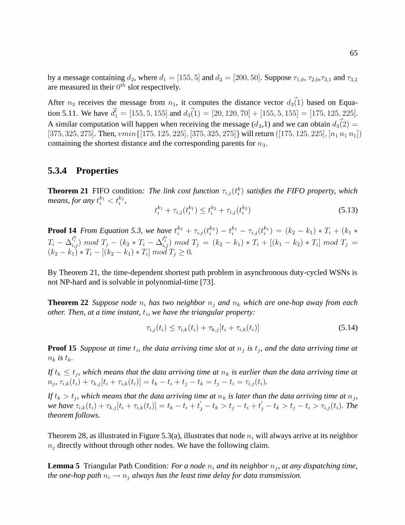
65

by a message containing d2, where d1 = [155, 5] and d2 = [200, 50]. Suppose τ1,0, τ2,0,τ3,1 and τ3,2

are measured in their 0th slot respectively.

After n3 receives the message from n1, it computes the distance vector �d3(1) based on Equa-tion 5.11. We have �d′

1 = [155, 5, 155] and �d3(1) = [20, 120, 70] + [155, 5, 155] = [175, 125, 225].A similar computation will happen when receiving the message (d2,1) and we can obtain �d3(2) =[375, 325, 275]. Then, vmin{[175, 125, 225], [375, 325, 275]}will return ([175, 125, 225], [n1 n1 n1])containing the shortest distance and the corresponding parents for n3.

5.3.4 Properties

Theorem 21 FIFO condition: The link cost function τi,j(tki ) satisfies the FIFO property, which

means, for any tk1i < tk2

i ,tk1i + τi,j(t

k1i ) ≤ tk2

i + τi,j(tk2i ) (5.13)

Proof 14 From Equation 5.3, we have tk2i + τi,j(t

k2i ) − tk1

i − τi,j(tk1i ) = (k2 − k1) ∗ Ti + (k1 ∗

Ti − Δt0ii,j) mod Tj − (k2 ∗ Ti − Δ

t0ii,j) mod Tj = (k2 − k1) ∗ Ti + [(k1 − k2) ∗ Ti] mod Tj =

(k2 − k1) ∗ Ti − [(k2 − k1) ∗ Ti] mod Tj ≥ 0.

By Theorem 21, the time-dependent shortest path problem in asynchronous duty-cycled WSNs isnot NP-hard and is solvable in polynomial-time [73].

Theorem 22 Suppose node ni has two neighbor nj and nk which are one-hop away from eachother. Then, at a time instant, ti, we have the triangular property:

τi,j(ti) ≤ τi,k(ti) + τk,j[ti + τi,k(ti)] (5.14)

Proof 15 Suppose at time ti, the data arriving time slot at nj is tj , and the data arriving time atnk is tk.

If tk ≤ tj , which means that the data arriving time at nk is earlier than the data arriving time atnj , τi,k(ti) + τk,j[ti + τi,k(ti)] = tk − ti + tj − tk = tj − ti = τi,j(ti).

If tk > tj , which means that the data arriving time at nk is later than the data arriving time at nj ,we have τi,k(ti) + τk,j[ti + τi,k(ti)] = tk − ti + t

′j − tk > tj − ti + t

′j − tk > tj − ti > τi,j(ti). The

theorem follows.

Theorem 28, as illustrated in Figure 5.3(a), illustrates that node ni will always arrive at its neighbornj directly without through other nodes. We have the following claim.

Lemma 5 Triangular Path Condition: For a node ni and its neighbor nj , at any dispatching time,the one-hop path ni → nj always has the least time delay for data transmission.

66

ni

nj

nkni

nj

nk

(a) (b)

Figure 5.3: Triangular path condition: the direct one-hop path ni → nj always achieve the leastlatency among all pathes from ni to nj.

Proof 16 We prove this by induction. Suppose there are multiple nodes along the path from n i tonj and define these nodes as nk, nk+1, · · · , nk+i. If i = 0, based on Theorem 28, Lemma 6 is true.

Now assume i = k and Lemma 6 is true. We prove that Lemma 6 is true when i = k + 1. Supposethe adjacent node to ni along the path is nk. Then the direct path nk → nj has shorter latencycomparing the path along nk+1, · · · , nk+i. Also based on Theorem 28, ni → nj has shorter latencythen the path ni− > nk− > nj . Therefore, the direct path ni → nj has shorter latency than thepath along nk, nk+1, · · · , nk+i. The lemma follows.

An illustration is given in Figure 5.3(b). Note that the triangular path condition does not exist instatic networks.

5.4 Algorithm for Initial Route Construction

We now present distributed algorithms for initial time-dependent shortest path route constructionin duty-cycled WSNs, where the distances from all nodes to the sink node are initially infinite.

The proposed algorithm referred to as the FTSP algorithm, Fast Time-Dependent Shortest Pathalgorithm, is inspired by existing algorithms [50], and is adapted from the distributed Bellman-Ford algorithm augmented with β-synchronizer [97]. Comparing with the solution in [50], whichonly computes the shortest paths for a given specified discrete time, FTSP compute the shortestpaths for infinite discrete time intervals in one execution.

Let |Dm| denote the diameter of the longest shortest path for all nodes. We show that the mes-sage complexity of FTSP is O(|Dm||E|) and the time complexity is O(|Dm||V |). FTSP does notsuffer from exponential message complexity, like in previous work [98] for the static shortest pathproblem over asynchronous networks.

5.4.1 Distributed Algorithm Description

We present the data structures and message formats in FTSP:

• �di: vector of distance from ni to ns, defined in Equation 5.8; initially all elements are∞;

67

• �τi,j: link delay from ni to its neighbor nj , defined in Equation 5.7; τi,j [0] is obtained by mea-surement;• �pi: vector of parents for ni in the shortest path ni → ns for infinite time intervals; initially allelements are node ni;• MSG(IDsrc, IDfrom, �d, updated): control message; IDsrc is the node ID of sink node, or up-date source node (see Section 5.5); IDfrom is the sender’s node ID; �d is the distance vector ofthe sender; updated is to show whether there is update in the current iteration, which will beexplained later;• ACK[j]: boolean indicating whether a node receives a control message from its neighbor nj

We assume that ni knows the duration of the checking interval Tj of all its neighbors nj ∈ Ni aftermeasuring link delays. Initially, a directed spanning tree rooted at ns is built upon the network. Weassume that ni knows its parent st pi in the spanning tree. We also assume that FTSP is invokedby higher-level protocols that create “START” impetuses at ns.

Algorithm 1: Algorithm for sink node ns in FTSP:Initialization:∀nj ∈ Ns, ACK[j] = 0, updated[j] = true;

On receiving START:send MSG(s, s, 0, false) to ∀nj ∈ Ns;

On receiving MSG(j, �dj , lj , bChanged):ACK[j] = 1; updated[j] = bChanged;if (∀nj ∈ Ns, ACK[j] == 1) then

ACK[j] = 0;if (∀nj ∈ Ns, updated[j] == false) then

STOP;else

send MSG(s, s, 0, false) to ∀nj ∈ Ns;

The first iteration of FTSP begins when node ns receives the “START” impetus. Subsequent onesbegin whenever ns completes an iteration and determines whether another one is necessary bychecking whether there is a node whose distance was minimized in the last iteration.

Each iteration begins at node ns by sending a control message to all its neighbors. When repliesfrom all its neighbors have been received, node ns concludes that an iteration is completed. Everyother node, i.e., ni (ni �= ns), begins an iteration upon receiving a control message from its parentst pi in the spanning tree, upon which it sends control messages to all its neighbors except st p i.When replies are received from all these neighbors, a control message is sent to the parent, therebycompleting the current iteration at node ni.

The control message from node nj contains the distance vector �dj (known thus far during theprevious iterations) between nj and ns. When such a message is received at node ni, node ni checkswhether the new information minish the value of any element in the current distance vector. It doesso by considering the path that goes through nj , taking into account the most recent informationfrom nj.

68

We describe the procedures in Algorithms 1 and 2.

Algorithm 2: Algorithm for node ni(i �= s) in FTSP:Initialization:st pi = NULL;for ∀nj ∈ Ni do

ACK[j] = 0; updated[j] = true;Measure link delay Δ0

i,j at the beginning of any time slot;l0i,j = the time slot number for measurement;lj = the data arriving time slot number at nj ;for ∀k ∈ [0..LCM(Ti, Tj)/Tj] do

τi,j [k] = Tj − (k ∗ Ti −Δ0i,j)mod Tj;

On receiving MSG(s, j, �dj , bChanged) from nj :

ACK[j] = 1; updated[j] = bChanged; �di

prev= �di;

if nj == st pi thensend MSG(s, i, �di, false) to ∀nj ∈ Ni except st pi;

�di(j) = vec add(�di, �dj , l0i,j , lj); /* Equation 5.11*/

(�di, �pi) = vmin(�di, �di(j)); /* Equation 5.12*/

if (�di�< �dprevi ) then updated[j] = true;

if (∀nj ∈ Ni, ACK[j] == 1) thenif (∃nj ∈ Ni, updated[j] == true) then bUpdated = true;else then bUpdated = false;send MSG(s, i, �di, bUpdated) to st pi;∀nj ∈ Ni, ACK[j] = 0;

The functions vec add(·), vmin(·), and operator �< are defined in Section 5.3.3.

5.4.2 Correctness and Complexity

Let PATH(i, tki ) be a path obtained by node ni, which is starting at time tki and moving along

its parent pi[k]. Let di[k]m denote the value of di[k] after the mth iteration in FTSP. We have thefollowing properties:

Theorem 23 1. After termination, PATH(i, tki ) is loop-free and concatenated; and 2. In the mth

(m ≥ 0) iteration, a node ni whose shortest path is at most m-hop away from the sink node for alldiscrete time intervals tk

i ∈ Ti will be determined.

Proof 17 For part 1, ∀tki ∈ Ti, after termination, suppose pi[k] is set to the node nj for the

shortest path with respect to ns. Since nj is the parent of ni at the time slot tki , PATH(i, tki ) is a

path composed of PATH(j, tki + τi,j(t

ki )) which is appended to node ni ∀tki ∈ Ti. Thus, for any

node ni and ∀tki ∈ Ti, PATH(i, tki ) is concatenated.

We prove that PATH(i, tki ) is loop-free by contradiction. Without loss of generality, assume that

there is a loop and the loop is (ni0 → ni1 → ni2 · · ·ni+k → ni0). This means that there is a

69

shortest path (ni0 → ni1 · · · ,→, ni+k), where ni+k is one-hop away from ni0 . According to thetriangular path condition in Lemma 6, such a shortest path cannot exist because n i0 → ni+k isalways the shortest one among all paths from ni0 to ni+k, contradicting the assumption.

We prove part 2 by induction on m. It is easy to find that the claim is true for m = 0. Now, assumethat the claim is true for m− 1 (i.e., the inductive hypothesis). We prove for m by induction.

Consider a specific time tki and a node ni such that there is a shortest path with at most m hops

between ni and ns. Let SP (i, s, tki , m) be the shortest path which is at most m hops from ni to ns

at time tki . Let nj be ni’s parent on SP (i, s, tk

i , m) at tki . This means that there is a path with atmost m− 1 hops between nj and ns.

By the inductive hypothesis, nj determined its shortest distance at the (m − 1)th iteration. In them-th iteration, node nj sends its minimized distance vector �djm−1 to node ni. Thus, SP (i, s, tki , m)

is determined after receiving the vector �djm−1 in the mth iteration, which completes the inductivestep. Since tki is chosen arbitrarily, this holds for all values of tk

i ∈ Ti.

The part 2 in Theorem 23 implies that, for m ≥ Dm, all nodes determine their minimum delay andthe corresponding parents for all time intervals, since all shortest paths contain at most Dm nodes.

Theorem 24 The message and time complexity of FTSP is O(Dm|E|) and O(Dm|V |) respectively.

Proof 18 Based on the implementation of the β-synchronizer in [99], in each iteration, there isexacted one message traversing each link in the spanning tree, totally |E| messages exchanged. ByTheorem 23, the number of iterations is upper bounded by the longest shortest path’s length Dm.Thus, the message complexity is O(Dm|E|).Suppose the largest delay for transmitting a message in the spanning tree is a constant, denotedby |C|. In each iteration, the time consumed is at most |V | ∗ |C|. Since there are at most Dm

iterations, the time complexity is O(Dm|V |).

5.5 Algorithm for Dynamic Route Maintenance

When compared with static networks, link changes and node changes are more frequent in duty-cycled WSNs. If a node changes its duty-cycle configuration, or dynamically joins or leaves thenetwork, the links connecting with all its neighbors will be changed at multiple time intervals. Insuch a situation, a single node update usually causes multiple link updates.

Some previous works (e.g., [77]) in static networks have proposed solutions that efficiently dealwith single link updates. They are inefficient for multiple link updates caused by a single nodeupdate. The algorithms in [77] are also memory-inefficient, since each node stores the route entriesfor all other nodes, incurring the space complexity of O(|V |).The proposed algorithms, referred as to FTSP-M (“M” meaning maintenance), focus on per nodeupdate and can be easily extended to node insertion and deletion. If there are multiple node updates,the algorithms will run concurrently at multiple nodes.

70

5.5.1 Distributed Algorithm Descriptions

The proposed distributed algorithms for path maintenance are also equipped with β−synchronizer.We use similar data structures and message formats as that in Section 5.4.1.

Suppose the source update node is nu and the corresponding input change is σ. We divide σ intotwo parts: σinc and σdec, where σinc includes the increasing links for ∀tk

u ∈ Tu, and σdec includesthe decreasing links for ∀tk

u ∈ Tu. Let δ(σinc) be the set of nodes that change either the distanceor the parents for all infinite discrete time intervals, as a consequence of σinc. Similarly, let δ(σdec)be the set of nodes affected by σdec. Apparently, δ(σ) = δ(σinc) ∪ δ(σdec).

FTSP-M consist of two phases for node nu and all nodes ni ∈ δ(σ) as described in Algorithms 3and 5.

In phase 1, an initial spanning tree is built up gradually to contain all nodes in δ(σ inc). The purposeof phase 1 is to let all nodes in δ(σinc) increase their distances to the sink node as a consequenceof σinc, along the time-expanded shortest path trees rooted at nu. After the termination of phase 1,all nodes in δ(σ) will never increase their distance again.

The rationale here is to satisfy the sufficient loop-free condition claimed in [100]: If at time t, nodeni detects a link-cost decrease or a decrease in the distance reported by a neighbor, then node ni isfree to choose its new parents. This is referred to as the distance increase condition (or DIC).

In each iteration, node nu sends a control message to all neighbors. Every other node, i.e., ni

(ni �= nu) will send control messages to all its neighbors if it is in the spanning tree and receives amessage from its parent. If ni is not in the spanning tree in the current iteration, it checks whethernj is its parent in its shortest path after receiving a control message from nj , which can be done bychecking whether nj ∈ �pi. If true, nv will join the spanning tree and set newspi = nj . By doingso, the spanning tree will increase at most one level in each iteration.

A control messages will traverse from the root (nu) to all other nodes in the spanning tree just likethat in FTSP. When node ni receives a control message from nj , it only updates the element to beincreased in its distance vector, as illustrated in Algorithm 4.

When replies from all its neighbors have been received, node nu concludes that an iteration iscompleted. When replies are received from all neighbors by a node, a control message is sent tothe parent, thereby completing the iteration at the node. When there is no distance increase for allnodes in δ(σinc), phase 1 will be terminated and node nu will start phase 2.

In phase 2, the initial spanning tree built up in phase 1 is continuously growing until it containsall nodes in δ(σ). Phase 2 is also running by iterations. In each iteration, when a node ni not inthe spanning tree receives a control message from nj , if the value of any elements in its distancevector can be minished, it will join the spanning tree by setting its parent newsp i to nj . Thedistance update and message traversing in phase 2 of FTSP-M are just similar to that in FTSP.

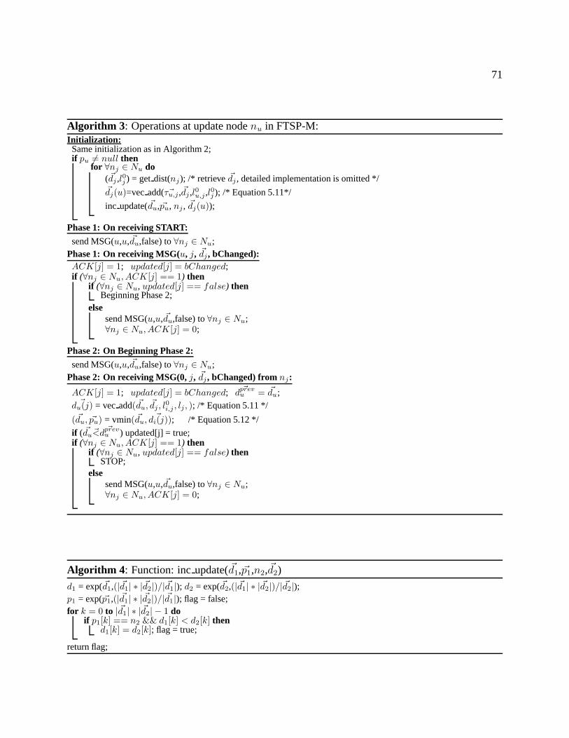
71

Algorithm 3: Operations at update node nu in FTSP-M:Initialization:Same initialization as in Algorithm 2;if pu �= null then

for ∀nj ∈ Nu do(�dj ,l0j ) = get dist(nj); /* retrieve �dj , detailed implementation is omitted */�dj(u)=vec add( �τu,j ,�dj ,l0u,j ,l0j ); /* Equation 5.11*/

inc update( �du, �pu, nj , �dj(u));

Phase 1: On receiving START:

send MSG(u,u, �du,false) to ∀nj ∈ Nu;Phase 1: On receiving MSG(u, j, �dj , bChanged):ACK[j] = 1; updated[j] = bChanged;if (∀nj ∈ Nu, ACK[j] == 1) then

if (∀nj ∈ Nu, updated[j] == false) thenBeginning Phase 2;

elsesend MSG(u,u, �du,false) to ∀nj ∈ Nu;∀nj ∈ Nu, ACK[j] = 0;

Phase 2: On Beginning Phase 2:

send MSG(u,u, �du,false) to ∀nj ∈ Nu;Phase 2: On receiving MSG(0, j, �dj , bChanged) from nj:

ACK[j] = 1; updated[j] = bChanged; �dprevu = �du;

�du(j) = vec add( �du, �dj , l0i,j , lj, ); /* Equation 5.11 */

( �du, �pu) = vmin( �du, �di(j)); /* Equation 5.12 */

if ( �du�< �dprevu ) updated[j] = true;

if (∀nj ∈ Nu, ACK[j] == 1) thenif (∀nj ∈ Nu, updated[j] == false) then

STOP;else

send MSG(u,u, �du,false) to ∀nj ∈ Nu;∀nj ∈ Nu, ACK[j] = 0;

Algorithm 4: Function: inc update( �d1,�p1,n2,�d2)

d1 = exp( �d1,(| �d1| ∗ | �d2|)/| �d1|); d2 = exp( �d2,(| �d1| ∗ | �d2|)/| �d2|);p1 = exp(�p1,(| �d1| ∗ | �d2|)/| �d1|); flag = false;for k = 0 to | �d1| ∗ | �d2| − 1 do

if p1[k] == n2 && d1[k] < d2[k] thend1[k] = d2[k]; flag = true;

return flag;

72

Algorithm 5: Operations in node ni(ni �= nu) in FTSP-M:Initialization: newspi = null; ∀nj ∈ Ni,updated[j] = false;Phase 1: On receiving MSG(u, j, �dj , bChanged) from nj:if nj ∈ Nu then

re-measure τi,u at the beginning of one time slot;reset l0i,j and l0u;

�di(j)=vec add( �τi,j ,�dj ,l0i,j ,l0j );if newspi == null then

if (inc update(�di,�pi,nj ,�di(j))) thennewspi = nj ; send MSG(u,i, �dj,true) to nj ;

else send MSG(u, i, �dj , false) to nj ;

elseFORWARD(u); /* u means the MACRO is executed in phase 1 */ACK[j] = 1; updated[j] = inc update( �di,�pi,nj ,�di(j));ACK REPLY(u);

Phase 2: On receiving MSG(0, j, �dj , bChanged):if newspi == null then

if (updated[j]) thennewspi = nj ; send MSG(0, i, �dj , true) to nj ;

else send MSG(0, i, �dj , false) to nj ;

elseFORWARD(0); /* 0 means the MACRO is executed in phase 2 */ACK[j] = 1; updated[j] = bChanged; �dprev

i = �di;�du(j) = vec add( �du, �dj , l

0i,j , lj); /* Equation 5.11*/

( �du, �pu) = vmin( �du, �di(j)); /* Equation 5.12*/

if ( �du�< �dprevu ) updated[j] = true;

ACK REPLY(0);FORWARD(int dict): code macroif (newspi == nj) then

send MSG(dict,i,�di,false) to ∀nj ∈ Ni except newspi;

ACK REPLY(int dict): code macroif (∀nj ∈ Ni, ACK[j] == 1) then

if (∃nj ∈ Ni, updated[j] == true) then bUpdated = true;else then bUpdated = false;send MSG(dict, i, �di,bUpdated) to newspi;∀nj ∈ Ni, ACK[j] = 1; bUpdated = false;

73

5.5.2 Correctness and Complexity

In phase 1, all nodes in δ(σinc) do not change their parents, but increase their distances as a conse-quence of σinc. Thus, there is no loop in phase 1. In phase 2, all nodes in δ(σ) will never increasetheir distances, thereby satisfying the distance increase condition [100]. All paths are thereforeloop-free.

Theorem 25 In phase 1, each node in δ(σinc) with at most m hops away from nu along the time-dependent shortest path will not increase its distance after m iterations.

Proof 19 The proof is through induction on m. It is easy to find that the claim is true for m = 0.Now, assume that the claim is true for m − 1 (i.e., the inductive hypothesis). We prove for m byinduction.

Consider a specific time tki and a node ni ∈ δ(σinc) such that there is a shortest path with at most

m − 1 hops between ni and ns after node update. Let SP (i, u, tki , m − 1) be the shortest path

which is at most m− 1 hops from ni to nu at time tki . Let nj be ni’s neighbor which is not updated

yet due to σinc. Then nj is at most m hops away from nu.

By the inductive hypothesis, ni will not increase its distance after (m − 1)th iteration. In the m-th iteration, node ni sends its updated distance vector �djm−1 to node nj , and nj will determineits updated distance in the iteration if nj ∈ δ(σinc). Thus, SP (j, u, tki , m) is determined afterreceiving the vector �dim−1 in the mth iteration, which completes the inductive step. Since tk

i ischosen arbitrarily, this holds for all values of tk

i ∈ Ti.

By Theorem 25, after |δ(σinc)| iterations, all nodes in δ(σinc) will not increase their distance any-more.

Definition 19 Updated-subpath: for any node ni ∈ δ, the updated-subpath is from ni to the firstnode ne not in δ along the shortest path from ni to nu.

Theorem 26 In phase 2, all generated updated-subpaths are loop-free, and updated-subpaths withat most m hops long are determined in the mth iteration.

Proof 20 After phase 1, the DIC loop-free condition [100] is satisfied. Thus, all updated-subpathsare loop free in phase 2.

The proof for at most m hops-long updated-subpaths being determined in the m th iteration can bedone by induction. It is easy to find that the claim is true for m = 0. Now, assume that the claim istrue for m− 1 (i.e., the inductive hypothesis). We prove for m by induction.

Consider a specific time tki and a node ni ∈ δ such that there is a updated-subpath which contains

m hops between ni and nu. Let UP (i, u, tki , m) be the updated-subpath which is at most m hopslong at time tk

i . Let nj be ni’s parent on UP (i, u, tki , m) at tki . This means that there is a updated-

subpath with at most m− 1 hops between nj and ns.

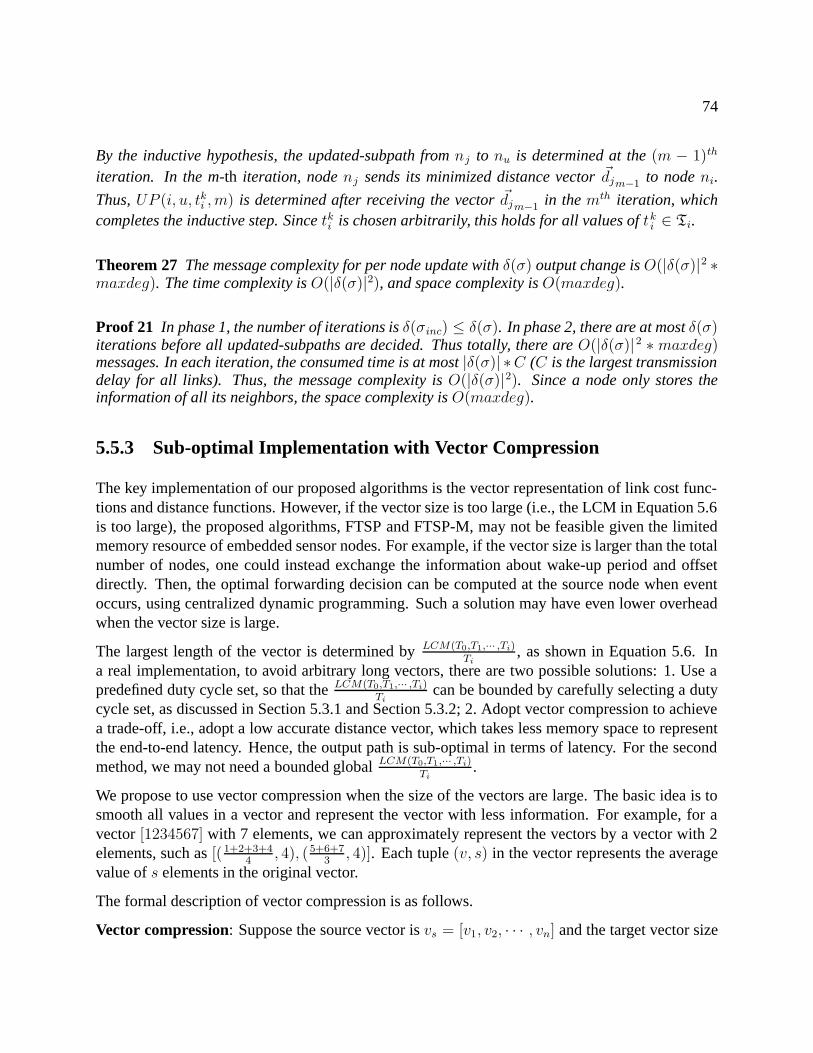
74

By the inductive hypothesis, the updated-subpath from nj to nu is determined at the (m − 1)th

iteration. In the m-th iteration, node nj sends its minimized distance vector �djm−1 to node ni.

Thus, UP (i, u, tki , m) is determined after receiving the vector �djm−1 in the mth iteration, whichcompletes the inductive step. Since tk

i is chosen arbitrarily, this holds for all values of tki ∈ Ti.

Theorem 27 The message complexity for per node update with δ(σ) output change is O(|δ(σ)|2 ∗maxdeg). The time complexity is O(|δ(σ)|2), and space complexity is O(maxdeg).

Proof 21 In phase 1, the number of iterations is δ(σinc) ≤ δ(σ). In phase 2, there are at most δ(σ)iterations before all updated-subpaths are decided. Thus totally, there are O(|δ(σ)|2 ∗ maxdeg)messages. In each iteration, the consumed time is at most |δ(σ)| ∗C (C is the largest transmissiondelay for all links). Thus, the message complexity is O(|δ(σ)|2). Since a node only stores theinformation of all its neighbors, the space complexity is O(maxdeg).

5.5.3 Sub-optimal Implementation with Vector Compression

The key implementation of our proposed algorithms is the vector representation of link cost func-tions and distance functions. However, if the vector size is too large (i.e., the LCM in Equation 5.6is too large), the proposed algorithms, FTSP and FTSP-M, may not be feasible given the limitedmemory resource of embedded sensor nodes. For example, if the vector size is larger than the totalnumber of nodes, one could instead exchange the information about wake-up period and offsetdirectly. Then, the optimal forwarding decision can be computed at the source node when eventoccurs, using centralized dynamic programming. Such a solution may have even lower overheadwhen the vector size is large.

The largest length of the vector is determined by LCM(T0,T1,··· ,Ti)Ti

, as shown in Equation 5.6. Ina real implementation, to avoid arbitrary long vectors, there are two possible solutions: 1. Use apredefined duty cycle set, so that the LCM(T0,T1,··· ,Ti)

Tican be bounded by carefully selecting a duty

cycle set, as discussed in Section 5.3.1 and Section 5.3.2; 2. Adopt vector compression to achievea trade-off, i.e., adopt a low accurate distance vector, which takes less memory space to representthe end-to-end latency. Hence, the output path is sub-optimal in terms of latency. For the secondmethod, we may not need a bounded global LCM(T0,T1,··· ,Ti)

Ti.

We propose to use vector compression when the size of the vectors are large. The basic idea is tosmooth all values in a vector and represent the vector with less information. For example, for avector [1234567] with 7 elements, we can approximately represent the vectors by a vector with 2elements, such as [( 1+2+3+4

4, 4), (5+6+7

3, 4)]. Each tuple (v, s) in the vector represents the average

value of s elements in the original vector.

The formal description of vector compression is as follows.

Vector compression: Suppose the source vector is vs = [v1, v2, · · · , vn] and the target vector size

75

is m (n > m). We compress vs by:

vt = [(v1 + v2 + · · ·+ vlen

len, len), (

v1+len + v2+len + · · ·+ v2∗lenlen

, len), · · · ,

(v1+(m−1)∗len + v2+(m−1)∗len + · · ·+ vn

n− (m− 1) ∗ len, n− (m− 1) ∗ len)]

where len = � nm.

We choose the average valuev1+i∗len+v2+len+···+v(i+1)∗len

lenas the value of vt[i] because the expected

deviation can be minimized by,

P =

len∑j=1

1

len|vt[i]− v[j]|

However, other filters, such as the Wavelet transform filter [101] can also be applied for vectorcompression, as typically done in image compression.

5.5.4 Further Discussions

The FTSP algorithm described in Section 5.4 is a proactive routing protocol. Although its timecomplexity is O(Dm ∗ |V |) for initial route construction, it is affordable in the initial stage ofWSNs. The low space complexity (O(|maxdeg|)) for route maintenance makes the algorithmscalable for large-scale WSNs.

Note that FTSP and FTSP-M target the ALPL mode [18] with various checking intervals. Whenall nodes have homogenous LPL checking intervals (like that in the standard B-MAC), accordingto Equations 5.3 and 5.5, the link cost function and the distance function will become constants. Insuch a case, our algorithms will default to the static shortest path algorithm. However, FTSP andFTSP-M will yield the same message complexities and time complexities for the static situation.

The dissertation focused on the scenario of single sink node. However, it can be extended to mul-tiple destinations. In WSNs, there is usually no end-to-end communication between two arbitrarynodes. We only consider the generalization of communication between one node and multiplesink nodes rather than the communication between two arbitrary nodes. In such a generalization,a node has to store the route information for all destinations (i.e., sinks). For each destination,our proposed algorithms can be applied for the route construction. Note that the delay property ismaintained for each individual destination in such an extension.

5.6 Experimental Results

We evaluated the performance of FTSP, FTSP-M, and the sub-optimal implementation throughextensive simulations using the OMNET++ discrete event simulator [102]. We compared our al-

76

gorithms against other related algorithms for the TDSP problem, including the distributed Bellman-Ford algorithm [98] adapted to the time-dependent model (Section 5.3), referred to here as TD-Bellman, and DSPP1 [50]. The following three major metrics were measured in the evaluation:1. message count; 2. time cost, which is the total time slots needed for stabilization; and 3. averagememory cost.

We examined two main factors that affect the performance of our algorithms, including networksize and underlying duty cycle setting. Our experimental settings were compatible with typicalconfigurations, as in [18, 39, 91]. The wireless communication range in our simulation was set to10m. We adopt the wireless loss model used in [103], which considers the oscillation of radiolinks. The size of the data packets was fixed as 512 bytes.

We generated 8 network size sets with varying sizes, G1,· · · ,G8, which are listed in Table 5.1.For each network size, we randomly generated 10 topologies. Each data point presented in ourexperimental results in this section is the average of 10 topologies, with 10 runs on each topology.

Table 5.1: Network Size SetsG1 G2 G3 G4|V | 50 80 200 400G5 G6 G7 G8|V | 600 1K 1.5K 2K

Table 5.2: Time slot setsC1 (ms) {100, 100, 100, 100}C2 (ms) {100, 200, 300, 600}C3 (ms) {100, 200, 400, 800}C4 (ms) {100, 200, 500, 1000}

We choose two MAC protocols: ALPL (adaptive low power listening) and quorum-based duty-cycling. The ALPL mode means that a node just wakes up for a short time during a checkinginterval to check the channel activities. The duration of the checking interval varies for differentnodes. We changed the duration of the checking interval in our simulation experiments with 4 sets,C1, C2, C3, and C4, as listed in Table 5.2. With each set, we randomly choose one element as thevalue of the LPL checking interval for each node.

Detector

Neighbor 1

Neighbor 2

beacon

wakeup slot

[2,3,5]

[3,4,6]

[3,6,7,12,14]

Figure 5.4: Quorum duty-cycling: detector with the quorum from (21,5,1)-difference set design,and neighbors with quorum from (7,3,1)-difference set design, as presented in [1].

For quorum-based duty-cycling, we choose the (7, 3, 1), and (21, 5, 1) difference sets for the het-erogenous wakeup schedule settings. The duration of one time slot was set to 100 ms in quorum-based duty-cycling. Since FTSP, FTSP-M, TD-Bellman, and DSPP1 are independent of wakeupscheduling, we argue that the comparison is fair even when we choose quorum-based duty-cycling.

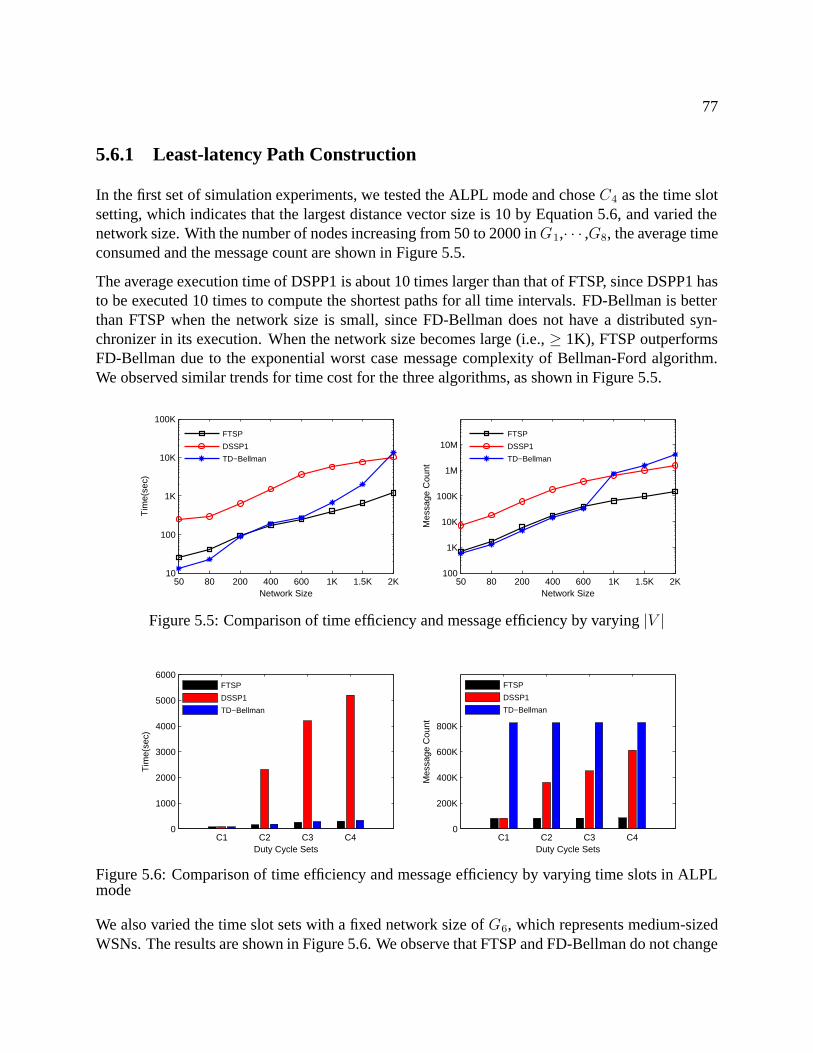
77

5.6.1 Least-latency Path Construction

In the first set of simulation experiments, we tested the ALPL mode and chose C4 as the time slotsetting, which indicates that the largest distance vector size is 10 by Equation 5.6, and varied thenetwork size. With the number of nodes increasing from 50 to 2000 in G1,· · · ,G8, the average timeconsumed and the message count are shown in Figure 5.5.

The average execution time of DSPP1 is about 10 times larger than that of FTSP, since DSPP1 hasto be executed 10 times to compute the shortest paths for all time intervals. FD-Bellman is betterthan FTSP when the network size is small, since FD-Bellman does not have a distributed syn-chronizer in its execution. When the network size becomes large (i.e., ≥ 1K), FTSP outperformsFD-Bellman due to the exponential worst case message complexity of Bellman-Ford algorithm.We observed similar trends for time cost for the three algorithms, as shown in Figure 5.5.

50 80 200 400 600 1K 1.5K 2K10

100

1K

10K

100K

Network Size

Tim

e(se

c)

FTSP

DSSP1

TD−Bellman

50 80 200 400 600 1K 1.5K 2K100

1K

10K

100K

1M

10M

Network Size

Mes

sage

Cou

nt

FTSP

DSSP1

TD−Bellman

Figure 5.5: Comparison of time efficiency and message efficiency by varying |V |

C1 C2 C3 C40

1000

2000

3000

4000

5000

6000

Duty Cycle Sets

Tim

e(se

c)

FTSP

DSSP1

TD−Bellman

C1 C2 C3 C40

200K

400K

600K

800K

Duty Cycle Sets

Mes

sage

Cou

nt

FTSP

DSSP1

TD−Bellman

Figure 5.6: Comparison of time efficiency and message efficiency by varying time slots in ALPLmode

We also varied the time slot sets with a fixed network size of G6, which represents medium-sizedWSNs. The results are shown in Figure 5.6. We observe that FTSP and FD-Bellman do not change

78

50 80 200 400 600 1K 1.5K 2K10

100

1K

10K

100K

Network Size

Tim

e(se

c)

FTSP

DSSP1

TD−Bellman

50 80 200 400 600 1K 1.5K 2K100

1K

10K

100K

1M

10M

Network Size

Mes

sage

Cou

nt

FTSP

DSSP1

TD−Bellman

Figure 5.7: Comparison of time efficiency and message efficiency for quorum-based duty-cyclesetting

their message count significantly since they only depend on the network size. The time cost ofall algorithms become worse when the average value of all elements in the selected time slot setbecomes larger, since the average link delay is correspondingly increasing.

Finally, we tested the performance for quorum-based duty-cycling by fixing the network size of G6.Each node randomly chose the (7, 3, 1) and (21, 5, 1) difference sets for its heterogenous schedulesettings. As shown in Figure 5.7, we observe similar trends for execution time and message count.The average execution time of DSPP1 is about 3 times larger than that of FTSP, since DSPP1 hasto be executed 3 times to compute the shortest paths for all time intervals given the (7, 3, 1) and(21, 5, 1) difference sets. The time costs for all the algorithms become worse when the networksize becomes larger, which is consistent with the conclusion in Theorem 24.

5.6.2 Least-latency Path Maintenance

For evaluating the path maintenance performance of FTSP-M, we return to static networks byselecting the time slot set of C1 in Table 5.2 for the ALPL mode. We do so for the purpose of afair comparison against previous works in [77], referred to here as Full-Dynamic and DSDV [104]with unicast support (multicast is not well-supported in duty-cycled WSNs).

We first evaluate the effect of input changes on all algorithms for medium-sized networks by choos-ing G6. Figure 5.8 shows the results. We observe that FTSP-M achieves the median message costand time cost when input changes become large. The reason is that DSDV may suffer exponentialmessage complexity. In addition, FTSP-M uses the synchronizer which consumes additional timeand messages, which is not as efficient as that in Full-Dynamic.

We also measure the average memory cost by varying the network size for the two underlying duty-cycling mechanisms. We first chose the ALPL mode and set the time slot set of C1 in Table 5.2for all nodes. The results shown in Figure 5.9 indicate that FTSP-M achieves the best memorycost, which does not depend on the network size. The memory costs of DSDV and Full-Dynamic

79

[1 10] [40 60] [80 100] [120 150] [150 200]

10

100

500

1000

#Nodes in input change

Tim

e(se

c)

FTSP−M

Full−Dynamic

DSDV

[1 10] [40 60] [80 100] [120 150] [150 200]10

100

1K

10K

100K

#Nodes in input change

Mes

sage

Cou

nt

FTSP−M

Full−Dynamic

DSDV

Figure 5.8: Performance comparison for route maintenance by varying input change: ALPL mode

50 80 200 400 600 1K 1.5K 2K

5

10

100

1000

5000

Network size

Mem

ory

(#en

trie

s) in

ALP

L M

ode

FTSP−M

Full−Dynamic

DSDV

50 80 200 400 600 1K 1.5K 2K

10

100

1000

5000

Network size

Mem

ory

(#en

trie

s) in

Quo

rum

−ba

sed

Dut

y−C

yclin

g M

ode

FTSP−M

Full−Dynamic

DSDV

Figure 5.9: Performance comparison for route maintenance on memory required in each node

increase with the network size, since each node stores an entry for all other nodes.

Finally, we tested the average memory cost for the quorum-based duty-cycling mechanism. Eachnodes randomly chose the (7, 3, 1) difference sets for the heterogenous schedule settings. As shownin Figure 5.9, we observe similar trends for the quorum-based duty-cycling mechanism. The onlydifference is that with (7, 3, 1) difference sets, each node maintains 3 entries in the routing tablefor all neighbors.

5.6.3 Performance of Sub-Optimal Implementation

For sub-optimal implementation with vector compression, the performance is a trade-off betweenpath latency and message size. We evaluated this tradeoff for both initial route construction androute maintenance. We first fixed the duty cycle setting by choosing C4 and compared the perfor-mance between FTSP and its sub-optimal implementation. Since the message count does not relyon vector implementation, we compared the vector size. Figure 5.10 shows the results. We ob-serve that the sub-optimal implementation achieves less message size with vector compression. To

80

understand the end-to-end latency of the two techniques, we compared the maximum value of theleast latency achieved by all nodes (defined as max-min latency). As shown in Figure 5.10, the sub-optimal implementation has higher max-min latency compared with FTSP. However, sub-optimalimplementation outperforms FTSP on average message size.

50 80 200 400 600 1K 1.5K 2K0

1000

2000

3000

4000

5000

Network Size

Max

−M

in L

aten

cy (

ms)

Sub−Optimal

FTSP

50 80 200 400 600 1K 1.5K 2K0

2

4

6

8

10

Network SizeV

ecto

r S

ize

Sub−Optimal

FTSP

Figure 5.10: Performance comparison for route construction: latency and vector size over ALPLmode

50 80 200 400 600 1K 1.5K 2K0

2000

4000

6000

8000

10000

12000

14000

Network Size

Max

−M

in L

aten

cy (

ms)

Sub−Optimal

FTSP

50 80 200 400 600 1K 1.5K 2K4

6

8

10

12

14

16

Network Size

Vec

tor

Siz

e

Sub−Optimal

FTSP

Figure 5.11: Performance comparison for route construction: latency and message size overquorum-based duty-cycling mode

We then fixed the duty cycle setting by choosing the (7, 3, 1) and (21, 5, 1) difference sets as thewakeup schedule for all nodes. We observed similar trends as shown in Figure 5.11. We observethat the sub-optimal implementation has higher max-min latency compared with FTSP, but has asmaller vector size.

5.7 Discussions

In this section, we discuss some practical implementation issues. In particular, we discuss how toachieve awareness of schedules of neighborhood nodes and how to reduce the vector size given a

81

large LCM in Equation 5.6.

FTSP and FTSP-M require awareness of wakeup schedules of the neighborhood. Achieving thisrequirement depends on the specific underlying MAC protocol. We discuss three scenarios forachieving schedule awareness over different MAC protocols.

Active Neighbor Discovery: This means that a node needs to probe the schedules of its neighborsactively. We consider two category of mechanisms, which needs active neighbor discovery. Oneis the LPL mode as adopted by B-MAC [13] and X-MAC [27]. The other is the low duty-cyclingmode where time axes are arranged as consecutive short time slots, and all slots have the sameduration Ts. In the low duty cycling mode, each node ni adopts a periodic wakeup schedule everyni time slots. The wakeup schedule can be once every ni (ni is an integer) slots. ni is called thecycle length for node ni. For example, in Figure 6.1(a), neighbor 1 has a schedule of {1, 0, 0},where 1 means wakeup slot and neighbor 2 has the schedule of {1, 0, 0, 0}. We assume that beaconmessages are send out at the beginning of wakeup slots, similar to [1, 85]. When a node wants todetect schedules of its neighborhood, it will wait until beacons are received from its neighbors.

The problem of configuring the schedule (i.e., the value of Li) has been studied in the past (e.g., [15]),and is outside the scope of this dissertation.

Quorum-based Duty-Cycling: In addition, FTSP and FTSP-M can be applied for asynchronousquorum-based wakeup scheduling [12] in wireless sensor/ad-hoc networks. In asynchronous wakeupscheduling, the neighbor discovery delay may vary at different time moments as illustrated in Fig-ure 5.12.

link delay= 1 (slot)

Node A

Node Blink delay= 0(slot) link delay= 7(slots)

data departure time t1 data departure time t2 t3

Figure 5.12: Varying neighbor discovery delay for quorum wakeup scheduling

The time-varying link cost function and the distance function are also periodic, and FTSP andFTSP-M are directly applicable.

Synchronization: MAC protocols with synchronization require that all neighboring nodes wakeup at the same time. The simplest method for doing this is to use a fully synchronized pattern,like that in the S-MAC protocol [23]. In this case, all nodes in the network wakeup at the sametime according to a periodic pattern. A further improvement can be achieved by allowing nodesto switch off their radio when no activity is detected for at least a timeout value, like that in theTMAC protocol [24]. In this scheme, neighboring nodes form virtual clusters to set up a commonsleep schedule. The main disadvantages of such scheduled neighbor discovery schemes are thecomplexity of implementation and the overhead for synchronization. Through synchronization, anode can conveniently know the schedules of its neighbors. Schedule awareness can be achievedby periodic message exchange between a node and its neighbors.

82

5.8 Conclusions

In this chapter, we addressed the distributed shortest path routing problem in duty-cycled WSNs.Our contributions are four-fold. First, we modeled duty-cycled WSNs as time-dependent networks,which satisfy the FIFO condition. Second, we presented FTSP algorithm for finding shortest pathsin such networks. FTSP has polynomial message complexity and is more time-efficient than previ-ous solutions. Third, we presented FTSP-M for distributed route maintenance with node insertion,updating, and deletion. FTSP-M is memory efficient and has polynomial message complexity. Fi-nally, we proposed a sub-optimal implementation in order to reduce the vector size. The vector sizeof the sub-optimal solution does not depend on the largest LCM value as shown in Equation 5.6.Experimental results validated the effectiveness and efficiency of our solutions.

We envision several directions for future work. One is to investigate the time-dependent minimumspanning tree problem, which is NP-Hard in duty-cycled WSNs. Another direction is to studytime-dependent multicast routing in duty-cycled WSNs, which is a required service for many ap-plications and is the reverse direction of all-to-one least-latency routing. And it is also valuable toconsider interference in the future research.

Chapter 6

Broadcast over Duty-Cycled WSNs

6.1 Motivations and Goals

Multihop broadcast [40] is an important network service in WSNs, especially for applicationssuch as code update, remote network configuration, route discovery, etc. Although the problem ofbroadcast has been well studied in always-on networks [41, 42] such as wireless ad hoc networkswhere neighbor connectivity is not a problem, broadcast is more difficult in duty-cycled WSNswhere each node stays awake only for a fraction of time slots and neighborhood nodes are not si-multaneously awake for receiving data. The problem becomes more difficult in asynchronous [12]and heterogenous duty-cycling [43] scenarios.

To support broadcast, synchronization of wakeup schedules is one promising approach adopted bymany duty-cycling MAC protocols, such as S-MAC [23] and T-MAC [24]. Such protocols simplifybroadcast communication by letting neighborhood nodes stay awake simultaneously. However,this approach results in high overhead for periodic clock synchronization when compared to thelow frequency of broadcast service in WSNs. Since energy is critical to WSNs, energy-efficientasynchronous MAC protocols have become increasingly attractive for data communication, asproposed in B-MAC [13], RI-MAC [85], Disco [63], and quorum-based wakeup scheduling [1,12].

However, previous asynchronous MAC protocols for duty-cycled WSNs mostly focus on unicastcommunication, and do not work well for broadcasting. One straightforward way to support one-hop broadcast in such cases is to deliver data multiple times for all neighbors, which results inredundant transmissions. With multihop broadcasting to an entire network, the problems are moreamplified, as some neighbors attempt to forward the broadcast message while the original trans-mitting node still attempts to transmit it to other nodes of its neighbors, increasing collisions andwasting energy consumption for transmission.

There have been some efforts in the past to support multihop broadcasting in duty-cycled WSNs.Wang et al. [83] transformed the problem into a shortest-path problem with the assumption of duty-cycle awareness, which is not valid for asynchronously duty-cycled WSNs. DIP [105], ADB [40],and opportunistic flooding [51] were designed with a smart gossiping approach. Essentially, these

83

84

protocols use unicast to replace broadcast for flooding, toward reducing the flooding latency in theentire network. However, they may lack efficiency in large-scale networks or on delivering largechunks of data to entire network because message cost and higher transmission energy consump-tion.

To overcome the disadvantages of replacement via pure unicast, we present Hybrid-cast, an asyn-chronous broadcast protocol for broadcasting with low latency and reduced message count. InHybrid-cast, a node only forwards a message to neighbors who wake up and send out beacon mes-sages. A node defers broadcasting by one or more time slot(s) after receiving the beacon messagefrom the first awake neighbor in order to wait for more nodes that may potentially wake up, sothat more nodes are accommodated in one broadcast. It also adopts online forwarder selection inorder to reduce the transmission redundancy. Compared with previous protocols, Hybrid-cast canachieve less broadcast latency and smaller message count.

Goals: Let us define the broadcast latency as the time between the beginning of a broadcast andthe time at which every node receives the broadcast message. Also, let us define the broadcastcount as the number of broadcasting via all nodes to ensure that the entire network receives themessage. Our goal is to design a broadcast schedule, which can not only shorten the broadcastlatency but also the broadcast count for flooding a message to the entire network. The protocol thatwe present, Hybrid-cast, is a heuristic solution to this problem.

6.2 Hybrid-cast Protocol

6.2.1 Overview

In Hybrid-cast, a transmitter will stay awake for long enough time to hear the beacon messagefrom its neighbors. Due to heterogenous wake-up scheduling, for low duty-cycling, the node willstay awake for Lm time slots, which is the largest cycle length of all neighbors. By doing this, itcan hear beacons from all neighbors. For quorum duty-cycling, the transmitter will switch to thewakeup schedules which has the largest cycle length from all its neighbors.

Hybrid-cast adopts opportunistic forwarding with delivery deferring to shorten broadcast latencyand broadcast count: the transmitter will forward the message within δ time after it hears thebeacon messages from early-wakeup neighbors, rather than forwarding immediately after hearingthe beacon messages. An illustration is given in Figure 6.1(a). Here, δ (i.e., δ = Ts for low duty-cycling) is called the deferring time. By deferring, the first-awake neighbor can still receive thebroadcast message. Meanwhile, more neighbors which wake up during the deferred time periodcan receive the broadcast message, so that less number of broadcast is necessary for one-hopbroadcasting.

To further reduce redundant transmissions, Hybrid-cast adopts online forwarder selection. “On-line” means that a node selects the least relay node among its instant one-hop awake neighbors,rather than all one-hop neighbors, to cover its two hop neighbors, in order to reduce transmission

85

redundancy and collision.

Transmitter

Receiver 1

Receiver 2

Receiver 3

(a) low duty-cycling (b) quorum duty-cycling

beacon

wakeup slot

broadcast broadcastbroadcast

[1,0,0]

[1,0,0,0]

[1,0]

Figure 6.1: Opportunistic broadcasting with delivery deferring (a) low duty-cycling case; (b) quo-rum duty-cycling case with wakeup schedules of [1,1,0,1,0,0,0] and its rotations which complywith (7,3,1) cqs design in [1].

6.2.2 Wakeup Schedule Switching

Due to adaptive duty-cycling, neighbor discovery becomes more difficult. In order to hear thebeacon message from all neighbors, a node must switch its wakeup schedule for staying awake forenough time slots.

For the case of low duty-cycling, in the idle state, a node ni follows its own wakeup schedule. Ifthe node needs to forward a broadcast message (i.e., the node is selected as a relay node), ni shouldstay awake for at least Lm slots, where Lm = maxnj∈N(i){Lj}. By doing this, ni can hear beaconmessages from all neighbors within the minimum necessary time slots.

For the case of quorum duty-cycling, ni just switches to the schedule of the node which has thelongest cycle length. Due to the non-empty intersection property [1], ni can still hear all neighborseven when it does not stay awake in every time slot of a whole cycle length.

A node needs to know the largest cycle length of its neighbors before schedule switching. This canbe achieved by either pre-setting the largest global cycle length or by dynamic neighbor informa-tion exchange protocols.

6.2.3 Opportunistic Forwarding with Deferring

Opportunistic forwarding means that a transmitter forwards data immediately to the neighborwhich wake up earlier, for minimizing broadcast latency. Previous efforts on opportunistic flood-ing such as [51] use unicast for broadcasting. However, opportunistic forwarding via pure unicastsuffers from large broadcast count.

In Hybrid-cast, broadcast deferring is adopted to minimize the one-hop broadcast count. By de-ferring, a transmitter will not broadcast messages immediately after receiving the beacon from thefirst-awake neighbor. In order to ensure that more neighbors receive the broadcast message, the

86

transmitter defers the broadcasting by δ = 1 time slot. By doing this, the first-awake neighborcan still receive the message, and the neighbors which wake up before the deferring time is duecan also receive the broadcast message. Thus, deferring combines the advantages of opportunisticforwarding and the advantages of broadcasting over wireless radio.

As shown in Figure 6.1, suppose there are three neighbors for the transmitter. The transmitter onlyneeds to broadcast two times (marked by the red arrow) to ensure that all neighbors will receivethe message. This is more efficient than the pure opportunistic forwarding mechanism.

The only disadvantages of deferring is the additional latency (1 time slot for one-hop broadcasting)for flooding to the entire network. Therefore, deferring allows the tradeoff between the numberof broadcast count and the broadcast latency to be exploited. We show in Section 6.3.2 that suchadditional latency is relatively small for the low duty-cycling case.

6.2.4 Online Forwarder Selection

In order to reduce the broadcast count or redundant transmission for multihop broadcasting, it isnecessary to select as small number of relay nodes as possible. Many past efforts have formulatedthis problem as the Minimum Connecting Dominating Set (MCDS) problem [106]. However,we argue that a static MCDS cannot be applied for relay node selection in Hybrid-cast. First, toshorten the latency, it is necessary to select the relay nodes or forwarders along the direction ofopportunistic forwarding, which results in online (or live) forwarder selection, rather than a statictopology control as done in MCDS. Secondly, MCDS does not achieve minimum broadcast countin asynchronous duty-cycled WSNs due to multiple delivery for single hop broadcasting.

Algorithm 6: Algorithm for all node nx:set Nawake(x);1:

N2reachable(x) = ∪y∈Nawake(x)N(y)−Nawake(x);2:

for ny ∈ Nawake(x) do3:if node nu ∈ N2

reachable(x) which is only reachable by ny then4:ny is selected into O-MPR(x);5:

N2reachable(x) = N2

reachable(x) − nu;6:

while N2reachable(x) �= ∅ do7:

for nu ∈ Nawake(x) - O-MPR(x) do8:nm = nu which covers the most nodes in N 2

reachable(x);9:

nm is selected into O-MPR(x);10:

N2reachable(x) = N2

reachable(x) - node set covered by nm;11:

In Hybrid-cast, initially, each node maintains its one hop awake neighbors (defined as N(x))and the set of two hop neighbors N 2(x) based on any underlying neighbor discovery protocols.The sink node or a relay node nx computes the least number of relay nodes among its one-hopawake neighbors (defined as Nawake(x)) to cover the reachable two hop neighbors (defined as

87

N2reachable(x)).

N2reachable(x) = ∪y∈Nawake(x)N(y)−Nawake(x) (6.1)

The main purpose of the online forwarder selection algorithm in a transmitter nx is to computeN2

reachable(x) as shown in Equation 6.1, and to compute the minimum number of relays to coverN2

reachable(x).

We adopt a heuristic solution, which is similar to the minimum multipoint relays (MPR) algorithmin [107]. The MPR problem is NP-Complete as shown in [107]. Thus, the minimum online for-warder selection problem is also NP-Complete. We denote the online MPR set for the transmitternx as O-MPR(x). We provide a heuristic algorithm for computing O-MPR(x) as described inAlgorithm 6. An illustration is given in Figure 6.2(a).

Let us define the delivery latency from node ni to node nj as the time between when the datais ready in ni and time at which the broadcast data is received by the neighbors, and denote thelatency as τi,j(t) at time t (τi,j(t) is varying at different time). We have the following property.

Theorem 28 Suppose node ni has two neighbor nj and nk which are one hop away from eachother. Then, at a time instant, ti, we have the triangular property:

τi,j(ti) ≤ τi,k(ti) + τk,j(ti + τi,k(ti)) (6.2)

Proof 22 Suppose at time ti, the data arriving time slot at nj is tj , and the data arriving time atnk is tk.

If tk ≤ tj , which means that the data arriving time at nk is earlier than the data arriving timeat nj , τi,k(ti + τk,j(ti + τi,k(ti)) = tk − ti + tj − tk = tj − ti = τi,j(ti). Otherwise, if tk > tj ,which means that the data arriving time at nk is later than the data arriving time at nj , we haveτi,k(ti) + τk,j(ti + τi,k(ti)) = tk − ti + t

′j − tk > tj − ti + t

′j − tk > tj − ti > τi,j(ti). The theorem

follows.

1st round

2nd round

3rd round

4th round

4th round

5th round

ni

nj

nkni

nj

nk

(b) (c)(a)

Figure 6.2: Online forwarder selection and the triangular path condition.

Theorem 28, as illustrated in Figure 6.2(b), illustrates that node ni will always broadcast data to itsone-hop neighbor nj directly, without through other nodes.

We also have the following property.

Lemma 6 Triangular Path Condition: For a node ni and its neighbor nj , at any time, the one-hopbroadcast latency ni → nj is always the minimum possible.

88

We omit the proof for the triangular path condition since it is a simple extension from that ofTheorem 6.2. An illustration is given in Figure 6.2(c). Note that the triangular path conditiondoes not exist in static networks. The triangular path condition indicates that the one-hop directbroadcast always achieves the least latency, in adaptively duty-cycled WSNs.

6.3 Performance Analysis

We now analyze the performance of Hybrid-cast in terms of the broadcast count and the broadcastlatency, in order to illustrate its design advantages.

6.3.1 Upper-Bound on One-Hop Broadcast Count

We consider two scenarios in analyzing the one-hop broadcast count. In the low duty-cyclingscenario, the schedule for a node ni is waking up once every Li time slots. In the quorum duty-cycling scenario, the schedule for a node ni is waking up q times for every Li consecutive timeslots, where q is the quorum size.

Lemma 7 [low duty-cycling] In Hybrid-cast, for a node ni, the broadcast count is at least one,and at most max{Δ, Lm}, where Δ is the node degree of ni and Lm is the maximum cycle lengthof nodes in the neighborhood.

Proof 23 If all nodes wake up within the same time slot, then after broadcast deferring, the trans-mitter can hear all neighbors, and one broadcast can cover all neighbors.

Otherwise, if Δ ≥ Lm, the transmitter can hear all neighbors via staying awake for Lm time slots.Therefore, the maximum broadcast count is Lm. If Δ < Lm, the transmitter can hear neighbors forat most Δ times, and the maximum broadcast count is Δ. Thus, the maximum number of broadcastcount is max{Δ, Lm}.

By the Lemma 7, the upper bound of broadcast count in Hybrid-cast is at most n (where n is thenetwork size) in the ideal case.

Lemma 8 [quorum duty-cycling] In Hybrid-cast, for node ni, the broadcast count is at least one,and at most max{Δ, qm}, where Δ is the node degree of ni and qm is the largest quorum size ofthe quorum systems adopted by nodes in the neighborhood.

Proof 24 If all nodes wake up within one time slot, then after broadcast deferring, the transmittercan hear all neighbors, and one broadcast can cover all neighbors.

Otherwise, if Δ ≥ qm, the transmitter can hear all neighbors via staying awake in time slotsscheduled by the quorum design. Therefore the maximum broadcast count is qm. If Δ < q, thetransmitter will hear neighbors for at most Δ times, and the maximum broadcast count is Δ. Thus,the maximum broadcast count is max{Δ, qm}.

89

6.3.2 Delivery Latency

Lemma 9 Suppose the depth of the network (i.e., maximum layers by breadth-first-search) isDmax. Then, the upper bound for delivery latency is Lm ∗ Dmax ∗ Ts in low duty-cycling mode,where Lm is the maximum cycle length of nodes in the network. The upper bound is qm ∗Dmax ∗Tsfor quorum duty-cycling mode, where qm is the largest quorum size of the quorum systems adoptedby all nodes in the network.

Proof 25 Based on the Triangular Path Condition in Lemma 6, a node always broadcasts a mes-sage to its one-hop neighbors directly. Thus, for one hop broadcasting, the latency is at mostLm ∗ Ts. After Lm ∗ Ts, all nodes in the first layer will receive the broadcast message. Therefore,after Lm ∗Dmax ∗ Ts time, all nodes in the network will receive the broadcast message.

6.4 Simulation Results

We simulated Hybrid-cast using the OMNET++ simulator [102] and compared it against ADB [40]and opportunistic broadcasting [51] (denoted as OppFlooding).

Our experimental settings were consistent with the configurations in [18, 51]. We set the wirelessloss rate as 0.1 and the duration of one time slot as 100 ms. The wireless communication rangewas set to 10m. We adopted the wireless loss model in [103], which considers the oscillation ofradio. The size of the broadcast message packets was fixed as 512 bytes.

We examined the two main factors that affect the performance of our algorithms, including networksize and duty-cycle setting. We generated a network with different number of nodes. For eachnetwork size, we randomly generated 10 topologies. Each data point reported in this section is theaverage of 10 topologies, with 10 runs on each topology. We varied the network size to understandits impact on the broadcast count and broadcast latency.

We measured the performance of the algorithms in a variety of duty cycle settings. For the lowduty-cycling scenario, we varied the duration of the total periodic cycle length from 2Ts to 10Ts togenerate heterogenous duty-cycling in a network for different nodes. For the quorum duty-cyclingcase, we choose the (7, 3, 1), (13, 4, 1), and (21, 5, 1) difference sets for the heterogenous schedulesettings. Since ADB, OppFlooding, and Hybrid-cast are independent of wakeup scheduling, weargue that the comparison is fair, even though ADB and OppFlooding do not explicitly supportquorum duty-cycling.

6.4.1 Broadcast Count

We first measure the broadcast count which is the total number of broadcasting for flooding amessage to the whole network. In this set of experiments, the network size was fixed by 200 nodes.The experimental results for different protocols are shown in Figure 6.3(a). In the low duty-cycling

90

case, Hybrid-cast outperforms ADB by approximately 50%, because of the less number of unicastsinvolved, due to the protocol’s deferring and online forwarder selection.

0.1 0.20 0.30 0.4

80

120

160

200

240

280

320

Duty Cycle Ratio (a) Low Duty−Cycling

Bro

adca

st C

ount

Hybrid−cast

ADB

OppFlooding

(7,3,1) (13,4,1) (21,5,1)40

80

120

160

200

240

280

320

Quourm−based Schedule(b) Quorum Duty−Cycling

Bro

adca

st C

ount

Hybrid−cast

ADB

OppFlooding

Figure 6.3: Performance comparison on broadcast count

For the quorum-based duty cycle setting, all nodes in the network chose homogenous quorumschedules. The setting was varied simultaneously for all nodes in different set of experiments.As shown in Figure 6.3(b), Hybrid-cast performs better since broadcasting are aggregated withinquorum slots in each cycle. For example, for the (7, 3, 1) setting (i.e., a node will stay awake at the1st, 2nd, and 4th slot on every 7 consecutive slots), there are at most 3 broadcasts to ensure that allneighbor nodes receive the broadcast message. However, for ADB and OppFlooding, the averageone-hop broadcast count was 5 or 6, given the average degree in the network that we configured.The results validate the performance analysis in Section 6.3.1.

6.4.2 Broadcast Latency

Figure 6.4(a) shows the broadcast latency (defined as the time from broadcast beginning to allnodes receiving the broadcast data). With deferring, Hybrid-cast has slightly higher latency thanADB and OppFlooding, by about 10%, when the duty cycle ratio is 0.4, and by about 5%, whenthe duty cycle ratio is 0.1. As shown in Figure 6.4(a), as the duty cycle ratio decreases, the dis-advantages of Hybrid-cast become more negligible, since the broadcast latency is more dominatedby neighbor discovery latency.

0.1 0.20 0.30 0.4

8

10

12

Duty Cycle Ratio (a) Low Duty−Cycling

Bro

adca

st L

aten

cy(s

ec)

Hybrid−cast

ADB

OppFlooding

(7,3,1) (13,4,1) (21,5,1)

10

20

30

40

Quourm−based Schedule(b) Quorum Duty−Cycling

Bro

adca

st L

aten

cy

Hybrid−cast

ADB

OppFlooding

Figure 6.4: Performance comparison on broadcast latency

91

For the case of quorum duty-cycling, as shown in Figure 6.4(b), we observe a similar trend as thatof low duty-cycling. The latencies for all three protocols tend to increase with larger quorum cycle.However, the latencies tend to converge to the same value when the quorum cycle increases. Thisis because, the neighbor discovery latency is approximately linearly increasing with quorum cycle,as shown in [1] The results also validate the performance analysis in Section 6.3.2.

6.4.3 Impact of Network Size

We also evaluated the impact of network size and heterogenous duty-cycling on message count andbroadcast latency. For the low duty-cycling case, each node randomly selected a duty cycle ratioin the range 0.1 to 0.4. For the quorum duty-cycling case, we chose the (7, 3, 1), (13, 4, 1), and(21, 5, 1) difference sets for the schedules of all nodes (the non-empty intersection property amongthese sets was proved in [1]). In the simulation experiments, we varied the network size from 200nodes to 1600 nodes.

200 400 600 800 1000 1200 1400 1600

200

400

600

800

Duty Cycle Ratio (a) Low Duty−Cycling

Bro

adca

st C

ount

Hybrid−cast

ADB

OppFlooding

200 400 600 800 1000 1200 1400 1600

200

400

600

800

Quourm−based Schedule(b) Quorum Duty−Cycling

Bro

adca

st C

ount

Hybrid−cast

ADB

OppFlooding

Figure 6.5: Broadcast count with different network size.

200 400 600 800 1000 1200 1400 16004

8

12

16

20

24

Duty Cycle Ratio (a) Low Duty−Cycling

Bro

adca

st L

aten

cy

Hybrid−cast

ADB

OppFlooding

200 400 600 800 1000 1200 1400 160012

16

20

24

28

32

36

40

Quourm−based Schedule(b) Quorum Duty−Cycling

Bro

adca

st L

aten

cy

Hybrid−cast

ADB

OppFlooding

Figure 6.6: Broadcast latency with different network size.

As shown in Figure 6.5, as the network size increases, the message count of Hybrid-cast and theother two solutions exhibit an increasing trend. This is because, more relay nodes will be selectedin larger networks. The same trend exists for broadcast latency as shown in Figure 6.6, as there aremore hops along the breadth-first-search tree. This is consistent with the analysis in Section 6.3.2.

We also evaluated the impact of network size for quorum-based duty cycle setting. We observedsimilar trends for the broadcast count and broadcast latency as that in the low duty-cycling setting.

92

The performance comparisons thus illustrate the performance tradeoff achieved by Hybrid-cast.

6.5 Discussions and Conclusions

Note that we do not assume local synchronization or duty-cycle awareness, which is required bypast works such as [51] and [83]. The assumption in Hybrid-cast is neighbor-awareness. Suchawareness can be achieved by neighbor discovery protocols, or by quorum-based duty-cycling [1].Each node will inform its neighbors after reconfiguration on the duty-cycling.

By adopting quorum duty-cycling, Hybrid-cast can be extended to mobile WSNs, because neigh-bor discovery is guaranteed within bounded time in quorum duty-cycling, as shown in [1].

Due to the problem of hidden terminal, it is possible that one node may receive broadcast messagesfrom two nodes simultaneously, which leads to collision. For reliable broadcasting, if a nodereceived the broadcast, it can set a mark field in the beacon message. By checking the beaconmessage from the neighbor, a transmitter can decide whether retransmission is necessary. We donot defer broadcast for retransmission. The transmitter could backoff a random period 0 ≤ t ≤ Ts

in order to avoid collision.

We do not explicitly consider reliability issues in Hybrid-cast. However, the traditional ACK andNACK mechanisms for reliable data transmission can be applied to Hybrid-cast to support reliablebroadcasting.

In this chapter, we designed an asynchronous broadcasting protocol, Hybrid-cast, for WSNs withadaptively low duty-cycling or quorum-based duty-cycling schedules. The main difficulty of thisproblem is that, sensor nodes are not time-synchronized and do not stay awake simultaneously.Hybrid-cast broadcasts messages to the neighbors who wake up early, in order to shorten thebroadcast latency. Previous solutions often use multiple unicasts for broadcasting, which incurshigh overhead. To overcome the disadvantages of such multiple unicasts, Hybrid-cast defers broad-casting to ensure that the number of awake neighbors is as large as possible. We also selected theminimum relay points online in order to reduce broadcast count and collisions.

We mathematically established the upper bound of broadcast count and broadcast latency fora given duty-cycling schedule. We compared the performance of Hybrid-cast with ADB andOppFlooding protocols. Our simulation results validated the effectiveness and efficiency of ourdesign.

Chapter 7

Prototype Implementations

We implemented a prototype system over Telosb [10] from Crossbow Technology and TinyOS 2.0distribution [93] to validate our algorithms and protocol design for asynchronous quorum-basedwakeup scheduling and neighbor discovery. We targeted to the application of real-time targettracking/monitoring over duty-cycled WSNs.

We changed the protocol stack of TinyOS [93] by integrating new protocols proposed by us into theoperating system. Two important metrics were measured for evaluation from the implementation:event-to-sink delay which indicates time between when a sentry node discovers a target and thetime at which a report arrives at sink node; and energy saving ratio which represents the ratio ofwakeup time to entire demonstration duration.

7.1 Hardware and Software Platform

Each node in the system adopted Crossbow TPR2400/2420 (“Telosb”) Mote [10] platform. Telosbis an open-source experimental platform developed and published by the University of California,Berkeley (“UC Berkele”). The platform provides an integrated processor (TI MSP430 microcon-troller) radio solution including a USB interface, 2.4 GHz radio, PCB antenna, sensor interfaces.The Telosb is the same as the TPR2400 except that it comes with a pre-installed environmen-tal sensor suite. It is a research platform upon which cutting edge experiments on new ideas insensor networks can be developed. The IEEE 802.15.4 compliant radio support built into theTelosb allows for communications with other 802.15.4 enabled platforms, including the commer-cial grade FCC/ARIB certified MICAz Mote. As an uncertified radio platform, the TPR2400/2420intended for research and lab studies. The Telosb is fully compatible with UC Berkeleys open-source TinyOS distribution [93].

We deployed almost 20 nodes in the prototype system development. The Figure 7.1 show theTelosb device we used and the architecture in the proto-type network system.

We programmed over Telosb via Cygwin environment. Basically, the development contains con-

93

94

(a) Telosb

PC

USB SeriaCommunicat

GUI

Telosb N …

Telosb 1

altion

Id =1

Telosb 2 Id =2…

(b) Software Architecture

Figure 7.1: Telosb and System Architecture in Implementations

figuration and programming. The main steps of programming a TelosB Mote through PC USBinterface is as follows: (1) Identify the COM port: Plug one TPR2400/2420 into a PC; Open aCygwin shell and type motelist. Then this command will find the COM port your TPR2400/2420is on; and (2) Compile the TinyOS Application: Change your directory to the CntToLedsAndRfmdirectory (inside a Cygwin window); Compile (type ‘make telosb’); and (3) Compile the program:type “make telosb reinstall,〈node ID〉 bsl, 〈N〉” in he Cygwin window, where 〈node ID〉 sets thenode address (optional) and 〈N〉 is an integer one less than the COM port number assigned to theTPR2400/2420. For example if the TelosB is assigned COM port 11, then the value of 〈N〉 wouldbe 10.

We did not implement the sensing function and did not contain any sensing unit in the TelosBdevice. In order to simulate the sensing and reporting process, we used a mobile TelosB to act as a“target”, which we referred as to the target node. The target node sent out radio periodically (onceevery 200 mill seconds). When a common sensor nodes detected the radio from the target nodes,it would send a report towards the sink node.

There was one sink node which communicated through USB port with a PC that acts as a centralmonitoring station. Other nodes, when detected the moving target, reported a message with theirown location to the sink node. When the sink node received the reports, it forwarded the message tothe PC monitoring software, where the location of the target was shown. The GUI of the monitoringsoftware is shown in Figure 7.2. The software which is developed over Windows by Visual Studio2005 contains 3 parts: target location area, performance area, and physical onsite monitoring.

Regarding the TinyOS [93], it is an open-source operating system designed for wireless embeddedsensor networks. The main feature of TinyOS is the component-based architecture which enablesrapid innovation and implementation while minimizing code size as required by the severe memoryconstraints inherent in WSNs. TinyOS’s component library includes network protocols, distributed

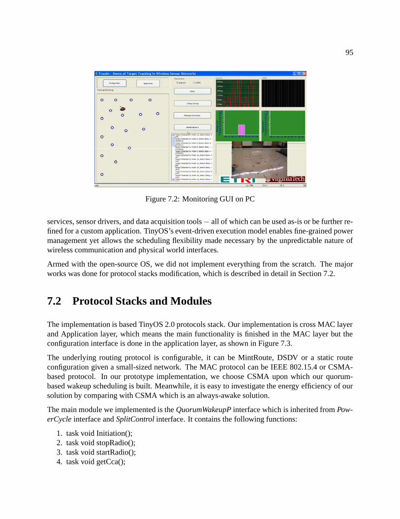
95

Figure 7.2: Monitoring GUI on PC

services, sensor drivers, and data acquisition tools− all of which can be used as-is or be further re-fined for a custom application. TinyOS’s event-driven execution model enables fine-grained powermanagement yet allows the scheduling flexibility made necessary by the unpredictable nature ofwireless communication and physical world interfaces.

Armed with the open-source OS, we did not implement everything from the scratch. The majorworks was done for protocol stacks modification, which is described in detail in Section 7.2.

7.2 Protocol Stacks and Modules

The implementation is based TinyOS 2.0 protocols stack. Our implementation is cross MAC layerand Application layer, which means the main functionality is finished in the MAC layer but theconfiguration interface is done in the application layer, as shown in Figure 7.3.

The underlying routing protocol is configurable, it can be MintRoute, DSDV or a static routeconfiguration given a small-sized network. The MAC protocol can be IEEE 802.15.4 or CSMA-based protocol. In our prototype implementation, we choose CSMA upon which our quorum-based wakeup scheduling is built. Meanwhile, it is easy to investigate the energy efficiency of oursolution by comparing with CSMA which is an always-awake solution.

The main module we implemented is the QuorumWakeupP interface which is inherited from Pow-erCycle interface and SplitControl interface. It contains the following functions:

1. task void Initiation();2. task void stopRadio();3. task void startRadio();4. task void getCca();

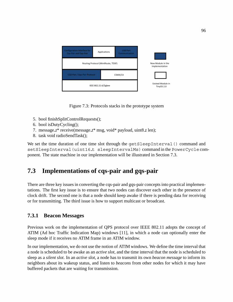
96

Routing Protocol (MintRoute, TDSP)

Configuration Interface forCqs Pair and Gqs Pair

USB PortCommunication

NewModule in theImplementation

Applications

IEEE 802.15.4/Zigbee

CSMA/CACQS Pair / Gqs Pair Protocol

Existed Module inTinyOS 2.0

Figure 7.3: Protocols stacks in the prototype system

5. bool finishSplitControlRequests();6. bool isDutyCycling();7. message t* receive(message t* msg, void* payload, uint8 t len);8. task void radioSendTask();

We set the time duration of one time slot through the getSleepInterval() command andsetSleepInterval(uint16 t sleepIntervalMs) command in the PowerCycle com-ponent. The state machine in our implementation will be illustrated in Section 7.3.

7.3 Implementations of cqs-pair and gqs-pair

There are three key issues in converting the cqs-pair and gqs-pair concepts into practical implemen-tations. The first key issue is to ensure that two nodes can discover each other in the presence ofclock drift. The second one is that a node should keep awake if there is pending data for receivingor for transmitting. The third issue is how to support multicast or broadcast.

7.3.1 Beacon Messages

Previous work on the implementation of QPS protocol over IEEE 802.11 adopts the concept ofATIM (Ad hoc Traffic Indication Map) windows [11], in which a node can optionally enter thesleep mode if it receives no ATIM frame in an ATIM window.

In our implementation, we do not use the notion of ATIM windows. We define the time interval thata node is scheduled to be awake as an active slot, and the time interval that the node is scheduled tosleep as a silent slot. In an active slot, a node has to transmit its own beacon message to inform itsneighbors about its wakeup status, and listen to beacons from other nodes for which it may havebuffered packets that are waiting for transmission.

97

awake sleepingquorum wakeup

schedule

data for transmiss

idle mode

more dtransmreceive

p gschedule

non-data for transm

awake

awake

quorum wakeup

sion active mode

data is mitting and er is awake more data is

transmitting and receiver is awake

awake

sleeping

schedule

mission

more data is transmitting and receiver is sleeping

Figure 7.4: Power Management at the Transmitter Side: Communication Schedule and Wakeupschedule

In our scheme, to ensure the correctness of the protocol, a node remains awake throughout its entireactive slot. It may be possible for nodes to be only partially awake during their active slots – suchoptimizations can be considered in future works. In a silent slot, a node will shut down its radio.

The beacon message contains three fields:{indic, node id, time stamp}. The indic field can haveonly two types of value: indic=0, which indicates that the message is a beacon message, and indic= 1, which indicates that the message is data. The node id field is used to distinguish amongdifferent nodes. The time stamp field is used to identify whether or not two beacon messages areidentical.

7.3.2 Power Management

The goal of power management is to facilitate effective communication while saving as muchenergy as possible. In our power management scheme, a node determines its desirable communi-cation schedule, i.e., when it should go to sleep or wake up. The relationship between the wakeupschedule and the communication schedule devised by a power management policy for a sender isillustrated in Figure 7.4.

At the MAC-layer, we propose a reservation mechanism for communication on top of the proposedquorum-based heterogenous wakeup scheduling scheme (cqs-pair or gqs-pair). Each node has twostates, idle mode and active mode. In the idle mode, a node will follow its wakeup schedule towake-up or to sleep. We also call this mode as power saving mode. Once there is data for receivingor for transmitting, the node will enter into the active mode as shown in Figure 7.4.

98

In the active mode, a sender maintains a table of timers for all its neighbors. The timers aretriggered once the sender receives beacon messages from the neighbors. The initial value of eachtimer is one time slot. The sender will also record its own wakeup schedule via a timer. If both thesender and the receiver is in an active slot, then they can communicate. If the sender enters intoa silent slot but there are more packets for transmission and the receiver is still in an active slot,then the sender will keep awake in its next slot. If there are more packets for transmission, but thereceiver will enter a silent slot, then the sender will send a keep-awake message to the receiver atthe end of the transmission of the current packet. The receiver that is being requested to stay awakewill then send back an acknowledgment, indicating its willingness to remain awake in its next slot.

The power management scheme at the receiver side is simpler than that at the sender side. In activemode, if there is no keep-awake message, the receiver will continue communication until the endof its current slot interval; otherwise, it will keep awake in its next slot.

7.3.3 Support for Multicast and Broadcast

Quorum-based asynchronous wakeup protocols cannot guarantee that more than one receiver isawake when a sender wishes to multicast or broadcast.

There are multiple ways to support multicast and broadcast. One method is to adopt relativelyprime frequencies among all nodes for wakeup scheduling. This method does not need synchro-nization between the sender and all the receivers. The sender only needs to notify m receivers towake-up via the pairwise relative primes p1, p2,..., pm, respectively. Then each receiver generatesits new wakeup frequency based on the received frequency. Through Chinese Remainder Theo-rem [68, 88], it can be proven that the m receivers must wakeup simultaneously at the I th beaconinterval (0 ≤ I ≤ p1 × p2...× pm). The sender can then transmit a multicast/broadcast message atthis interval.

Another way to multicast/broadcast is by using synchronization over quorum-based wakeup sched-ules. The sender can book-keep all neighbors’ schedules, and synchronize their schedules so thatneighboring nodes wake up in the same set of slots with the use of Lamport’s clock synchroniza-tion algorithm [108]. When all nodes are awake simultaneously, the senders then send a messageto multiple neighbors simultaneously.

The first mechanism has the advantage that no synchronization is needed between a sender andmultiple receivers. But it cannot bound the average delay. The second approach can bound the av-erage delay but it needs book-keeping and synchronization over asynchronous wakeup schedules.

For multicast/broadcast, we set a threshold L. If the number of multicast packets exceed thethreshold L, the sender will send a Multicast-Notify to all neighbor receivers, requesting them tostay awake. Otherwise the sender will send the multicast data to each receiver one by one, byunicasting. The value of the threshold L depends on the configuration of time slot lengths andpacket lengths.

99

(a) Line Topology (b) Performance Comparison (Upper:End-to-end la-tency; Below:Energy consumption ratio)

Figure 7.5: Performance Comparison for Line Topology

To reduce the time of waiting before actual transmission, the Multicast-Notify message contains afield to notify all receivers on how long they should wait. The value of this field is the time betweenwhen the message is sent and when all receivers are awake.

7.4 Demo Performance

(a) Tree Topology (b) Performance Comparison (Upper:End-to-end la-tency; Below:Energy consumption ratio)

Figure 7.6: Performance Comparison for Tree Topology

In the proto-type implementation, performance regarding energy saving ratio and e2e latency werecompared between Quorum-based wakeup scheduling and CSMA protocol. The application run-

100

ning was target tracking. We adopt two topologies for the comparisons: line topology and treetopology. We show below the live performance comparison in our demonstration before.

From the demonstration with both line topology and tree topology, we observe that there is atradeoff between the two mechanisms. As shown in Figure 7.5, although Quorum-based wakeupscheduling achieved less energy consumption ratio, but it suffered higher latency compared withCSMA protocol.We set the time slot length as 100ms in the Quorum-based wakeup scheduling, andselect the (7,3,1)-difference set design. When the hop count is 8, the end-to-end latency is almostover 2000ms for the Quorum scheme, but only about 500ms for CSMA protocol. However, theQuorum scheme only stay awake 42.8% time in idle state, comparing 100% for CSMA protocol.The similar trend existed for tree topology, as shown in Figure 7.6.

The demonstration performance verifies the design trade-off in the cqs-pair and gqs-pair protocols.Thus, when saving energy is an critical issue for sensor nodes, we should sacrifice the latency inorder to prolong the node lifetime individually.

Chapter 8

Conclusions and Future Work

This dissertation is motivated by saving idle energy consumption, providing optimal data routingin terms of E2E latency, and supporting efficient multihop broadcasting in duty-cycled WSNs. Thework is based on the observation that idle energy consumption for sensor nodes is not negligiblefor a large class of WSN applications (e.g., environment monitoring [4], target tracking [5]). Thedissertation adopts the duty-cycling approach for saving idle energy. However, this raises newchallenges on neighbor discovery, data delivery with optimal latencies, and data broadcasting.Toward this, the dissertation focuses on, and solves three problems: a) asynchronous wakeupscheduling and the corresponding neighbor discovery mechanism, b) time-varying shortest pathrouting due to varying link costs, and c) efficient multihop broadcast.

Our solutions on asynchronous wakeup scheduling were inspired by the quorum-based power sav-ing mechanism [11]. We proposed two designs, cqs-pair and ggs-pair, and provide a generalframework in which we can satisfy the heterogenous energy saving requirement, while guaran-teeing neighbor discovery latency. We show that this generalization is a non-trivial extension frompast works.

Armed with the design rationale (described in Chapter 4) of quorum systems, we first proposedcqs-pair, which guarantees that two adjacent nodes which adopt heterogenous cyclic quorums fromsuch a pair as their wakeup schedules, can hear each other at least once within one super cyclelength (i.e., the larger cycle length in the cqs-pair). We also developed a fast algorithm for con-structing cqs-pairs, using the multiplier theorem [44] and the (N, k, M, l)-difference pair definedby us. With the help of the cqs-pair, WSNs can achieve better trade-off between energy consump-tion and average delay. For example, all cluster-heads and gateway nodes in a heterogenous WSNcan select a quorum from the quorum system with smaller cycle length as their wake up schedules,to obtain smaller discovery delay. In addition, all members in a cluster can choose a quorum fromthe quorum system with longer cycle length as their wakeup schedules, in order to save more idleenergy. cqs-pair is the first asynchronous wakeup scheduling algorithm for heterogenous energysaving and meanwhile guaranteeing bound neighbor discovery latency over WSNs.

Another design that we propose on heterogenous quorum-based wakeup scheduling is gqs-pair, in

101

102

which each quorum system of the pair is a grid quorum system [45]. We prove that any two gridquorum systems can form a gqs-pair. Compared with cqs-pair, gqs-pair has better performance interms of average neighbor discovery latency. With the help of the gqs-pair, WSNs can also achievebetter tradeoff between energy consumption and average delay. Meanwhile, gqs-pair has betterperformance in terms of average neighbor discovery latency than cqs-pair.

We see from cqs-pair and gqs-pair that the quorum design can be applied as a framework for asyn-chronous wakeup scheduling in order to save energy in heterogenous WSNs. The framework canachieve tradeoff between energy saving ratio and discovery latency, and hence provide configura-tion flexility for different applications which are either energy-critical or latency-critical.

We also considered asymmetric quorum design to further improve the energy efficiency in two-tiered WSN topologies. We developed a flexible solution, p-Grid, for neighbor discovery service inlow duty-cycled WSNs. The motivation behind p-Grid was to provide an energy-efficient, run-timeconfigurable, asynchronous neighbor discovery mechanism for WSNs in unreliable environments.p-Grid is easy to implement: in idle state, nodes select a read quorum from a prime-grid quorumgroup as their low power listening schedules. For neighbor discovery, a node switches from lis-tening mode to probing mode by selecting a write quorum from a prime-grid quorum group asits probing schedule, and sends out DISC messages in the time slots selected as a write quorum.Armed with the prime-grid quorum group design, there must be at least one overlapping slot inwhich both the probing node and its neighbors in listening mode are awake simultaneously.

Therefore, p-Grid achieves better energy efficiency for neighbor discovery in unreliable environ-ments, compared with conventional protocols. We conclude from p-Grid protocol that asymmetricdesign on asynchronous wakeup scheduling can further improve the energy efficiency when thereis no data communication between cluster members (which is true for most of WSNs applications,like target tracking [5] and environment monitoring [4]).

The designs of cqs-pair, gqs-pair, and p-Grid constitute the first contribution in the dissertation.

The second contribution of the dissertation is time-dependent shortest path routing in duty-cycledWSNs. We model duty-cycled WSNs as time-dependent networks, which satisfy the FIFO condi-tion. We then developed the FTSP distributed algorithm for finding shortest paths in such networks.FTSP has polynomial message complexity and is more time-efficient than previous solutions. Wealso developed the FTSP-M algorithm for distributed route maintenance with node insertion, con-figuration updating, and deletions. FTSP-M is memory efficient and has polynomial messagecomplexity. Finally, we developed a sub-optimal implementation of FTSP and FTSP-M in orderto reduce the vector size. The vector size of the sub-optimal implementation does not depend onthe largest LCM value as shown in Equation 5.6.

Comparing with past works [50], the algorithms proposed by us have lower time and messagecomplexities in the worst case. And the number of execution times for enumerating shortest pathsfor all discrete time moments is bounded.

Our work on this part indicates that adaptively duty-cycled WSNs exhibits an unique time-dependentfeature: periodically varying link costs. Based on the periodical feature, the construction of

103

time-dependent shortest paths can be expedited largely compared with that for traditional time-dependent networks.

The dissertation’s third contribution is our solution for multihop broadcast in duty-cycled WSNs,which is an important service for many WSN applications, such as configuration update, messageflooding, route discovery etc. Toward this, we proposed Hybrid-cast. The main difficulty in thedesign of a multihop broadcast protocol in duty-cycled WSNs is that, sensor nodes are not time-synchronized, and therefore, do not stay awake simultaneously. Hybrid-cast broadcasts messagesto the neighbors who wake up early, in order to shorten the broadcast latency. Previous solutionsoften use multiple unicasts for broadcasting, which incurs high overhead. To overcome the disad-vantages of such multiple unicasts, Hybrid-cast defers broadcasting to ensure that the number ofawake neighbors is as large as possible. We also selected the minimum relay points online, in orderto reduce broadcast count and collisions. We analytically established the upper bound of broadcastcount and broadcast latency for a given duty-cycling schedule.

Comparing with previous solution (i.e., pure opportunistic flooding [51], and unicast replacementapproach [40]), Hybrid-cast achieves better tradeoff between broadcast latency and broadcast countcompared to previous broadcast solutions. Meanwhile, it reduces redundant transmission via de-livery deferring and online forwarder selection.

Hybrid-cast protocol reveals that the broadcast count can be largely reduced with small sacrificein broadcast latency which is critical for energy saving. Hence, some broadcast services withoutsensitive timeline requirement, such as code update and reconfiguration over duty-cycled WSNs,would benefit from it.

The dissertation’s fourth and last contribution is the prototype system development over real hard-ware and software platform. We implemented cqs-pair and gqs-pair in a WSN platform comprisedof Telosb [10] motes running TinyOS 2.0. The cqs-pair and gqs-pair designs were integrated withthe existing protocol stacks in TinyOS 2.0. We measured the performance of the designs in termsof energy-saving ratio and neighbor discovery latency, to show the superiority of our designs. Ourimplementation did not modify the upper layer routing protocols, and is pluggable to the existingsoftware architecture and protocol stack in TinyOS.

We conclude from the implementation that our solutions for quorum-based wakeup scheduling canbe applied to real WSN platforms with desired performance, and that the implementation of thosesolutions can work well with existing protocol stack and software modules.

8.1 Summary of Contributions

To summarize, the dissertation’s contributions include:

• We developed a set of asynchronous quorum-based wakeup scheduling schemes in duty-cycled WSNs including cqs-pair, ggs-pair, and p-Grid, and show that they provide a better

104

trade-off between energy consumption and average delay, and better energy efficiency forneighbor discovery in unreliable environments, compared with existing protocols.

• We modeled duty-cycled WSNs as time-dependent networks, and developed the FTSP andFTSP-M distributed algorithms for finding shortest paths in such networks. We show thatFTSP and FTSP-M algorithms are superior to past solutions.

• We developed a multihop broadcast protocol called Hybrid-cast for broadcasting in duty-cycled WSNs. Hybrid-cast upper bounds the broadcast count and broadcast latency for agiven duty-cycling schedule. We establish the superiority of Hybrid-cast over past solutions.

• We developed a prototype implementation of the cqs-pair and gqs-pair asymmetric quorumdesigns in a Telosb/TinyOS WSN platform. The implementation validate the feasibilityover existing WSN platforms. The experimental measurements show the superiority of overdesigns over existing solutions.

8.2 Future Work

Based on the dissertation’s results, we envision the following directions as promising avenues forfurther research.

One direction is to consider a general framework for adopting quorum systems in asynchronouswakeup scheduling. In the dissertation, we only discussed two quorum systems, cyclic quorum sys-tems and grid quorum systems. However, it may be possible to design better quorum systems whichcan be utilized for designing asynchronous wakeup scheduling schemes in duty-cycled WSNs. Ageneral framework for designing such schemes is desirable, which can provide a systematic viewand deeper insights on quorum systems that can yield greater energy savings or optimized E2Elatencies.

Another possible direction is capacity maximization. Although asynchronous quorum-based wakeupscheduling is energy efficient, it does not consider the collision during simultaneous transmis-sion to same receivers, which can happen frequently during data aggregation. Such collisions cansignificantly degrade the capacity and throughput. Existing asynchronous mechanisms, such asRTS/CTS, are not efficient for this problem. Scheduled transmission is one promising solution,but it requires clock synchronization. Hence, a protocol which combines the merits of both asyn-chronous protocols and synchronized protocols (or a hybrid solution), or some improved versionswith random quorum selection, or practical back-off time setting would be a promising line ofresearch for capacity maximization in data aggregation WSN applications.

Several interesting future research directions also exist in the problem space of time-varying E2Edata delivery in duty-cycled WSNs. Building upon the dissertation’s solutions on the time-dependentshortest path routing problem, one can consider the time-dependent minimum spanning tree prob-lem, which is NP-Hard, or consider improving existing routing protocols (i.e., minimum-hop rout-ing) with time-varying optimal latencies. Another very interesting direction is the time-dependent

105

multicast routing problem, which is the reverse direction of all-to-one routing discussed in thedissertation. Last but not least, we believe that it is worthy of considering interference in thetime-varying routing, which is probably one new research problem.

Bibliography

[1] S. Lai, B. Zhang, B. Ravindran, and H. Cho, “Cqs-pair: Cyclic quorum system pair forwakeup scheduling in wireless sensor networks.” in International Conference on Principlesof Distributed Systems (OPODIS), vol. 5401. Springer, 2008, pp. 295–310.

[2] I. F. Akyildiz, W. Su, Y. Sankarasubramaniam, and E. Cayirci, “Wireless sensor networks:a survey,” Computer Networks, vol. 38, pp. 393–422, 2002.

[3] G. Platt, M. Blyde, S. Curtin, and J. Ward, “Distributed wireless sensor networks and in-dustrial control systems - a new partnership,” in Proceedings of the 2nd IEEE workshop onEmbedded Networked Sensors (EmNets05: ), Washington, DC, USA, 2005, pp. 157–158.

[4] A. Mainwaring, D. Culler, J. Polastre, R. Szewczyk, and J. Anderson, “Wireless sensornetworks for habitat monitoring,” in Proceedings of the 1st ACM international workshop onWireless sensor networks and applications (WSNA02: ), 2002, pp. 88–97.

[5] T. He, P. Vicaire, T. Yan, L. Luo, L. Gu, G. Zhou, R. Stoleru, Q. Cao, J. A. Stankovic,and T. Abdelzaher, “Achieving real-time target tracking using wireless sensor networks,”in Proceedings of the 12th IEEE Real-Time and Embedded Technology and ApplicationsSymposium (RTAS06), 2006, pp. 37–48.

[6] J. A. Stankovic, Q. Cao, T. Doan, L. Fang, Z. He, R. Kiran, S. Lin, S. Son, R. Stoleru,and A. Wood, “Wireless sensor networks for in-home healthcare:,” in Proceeding of HighConfidence Medical Devices, Software, and Systems (HCMDSS05), 2005, pp. 2–3.

[7] K. Romer and F. Mattern, “The design space of wireless sensor networks,” Wireless Com-munications, IEEE, vol. 11, no. 6, pp. 54 – 61, Dec. 2004.

[8] L. M. Feeney and M. Nilsson, “Investigating the energy consumption of a wireless net-work interface in an ad hoc networking environment,” in IEEE Conference on. ComputerCommunications (INFOCOM), 2001, pp. 1548–1557.

[9] T. I. (TI), “Cc2420 data sheet,” http://focus.ti.com/lit/ds/symlink/cc2420.pdf.

[10] Crossbow, “Telosb datasheet,” http://www.xbow.com/Products/Product pdf files/Wirelesspdf/TelosB Datasheet.pdf.

106

107

[11] C. H. Y. Tseng and T. Hsieh, “Power-saving protocols for ieee 802.11-based multi-hop adhoc networks,” in IEEE Conference on. Computer Communications (INFOCOM), 2002, pp.200 – 209.

[12] R. Zheng, J. C. Hou, and L. Sha, “Asynchronous wakeup for ad hoc networks,” in Proceed-ings of the ACM symposium on Mobile ad hoc networking and computing (MobiHoc), 2003,pp. 35–45.

[13] J. Polastre, J. Hill, and D. Culler, “Versatile low power media access for wireless sensornetworks,” in Proceedings of the 2nd international conference on Embedded networkedsensor systems (Sensys), 2004, pp. 95–107.

[14] T. Voigt, H. Ritter, and J. Schiller, “Utilizing solar power in wireless sensor networks,” inProceedings of the 28th Annual IEEE International Conference on Local Computer Net-works (LCN), 2003, p. 416.

[15] C. Vigorito, D. Ganesan, and A. Barto, “Adaptive control of duty cycling in energy-harvesting wireless sensor networks,” in IEEE Communications Society Conference on Sen-sor, Mesh and Ad Hoc Communications and Networks (SECON), June 2007, pp. 21–30.

[16] J. A. Paradiso and T. Starner, “Energy scavenging for mobile and wireless electronics,” IEEEPervasive Computing, vol. 4, no. 1, pp. 18–27, 2005.

[17] A. Kansal, J. Hsu, S. Zahedi, and M. B. Srivastava, “Power management in energy harvest-ing sensor networks,” ACM Trans. Embed. Comput. Syst., vol. 6, no. 4, p. 32, 2007.

[18] R. J., P. B., and C. V., “Adaptive low power listening for wireless sensor networks,” IEEETransactions on Mobile Computing, vol. 6, no. 8, pp. 988–1004, 2007.

[19] C. Schurgers, S. G. V. Tsiatsis, and M. Srivastava, “Topology management for sensor net-works: Exploiting latency and density,” in ACM International Symposium on Mobile AdHoc Networking and Computing (MobiHoc), 2002.

[20] M. J. Miller and N. H. Vaidya, “Power save mechanisms for multi-hop wireless networks,” inProceedings of the First International Conference on Broadband Networks (BROADNETS),2004, pp. 518–526.

[21] L. Gu and J. Stankovic, “Radio-triggered wake-up capability for sensor networks,” in Pro-ceedings of the 10th IEEE Real-Time and Embedded Technology and Applications Sympo-sium (RTAS), 2004, pp. 27–37.

[22] Y. Sun, S. Du, O. Gurewitz, and D. B. Johnson, “Dw-mac: a low latency, energy effi-cient demand-wakeup mac protocol for wireless sensor networks,” in Proceedings of the 9thACM international symposium on Mobile ad hoc networking and computing (MobiHoc08:), 2008, pp. 53–62.

108

[23] W. Ye, J. Heidemann, and D. Estrin, “Medium access control with coordinated adaptivesleeping for wireless sensor networks,” IEEE/ACM Transactions on Networking (TON),vol. 12, pp. 493–506, 2004.

[24] T. Dam and K. Langendoen, “An adaptive energy-efficient mac protocol for wireless sensornetworks,” in The First ACM Conference on Embedded Networked Sensor Systems (Sensys),2003.

[25] Q. Cao, T. Abdelzaher, T. He, and J. Stankovic, “Towards optimal sleep scheduling in sensornetworks for rare-event detection,” in Proceedings of the 4th international symposium onInformation processing in sensor networks (IPSN), 2005.

[26] A. Keshavarzian, H. Lee, and L. Venkatraman, “Wakeup scheduling in wireless sensor net-works,” in Proceedings of the 7th ACM international symposium on Mobile ad hoc network-ing and computing (MobiHoc), 2006, pp. 322–333.

[27] M. Buettner, G. V. Yee, E. Anderson, and R. Han, “X-mac: a short preamble mac protocolfor duty-cycled wireless sensor networks,” in Proceedings of the 4th international confer-ence on Embedded networked sensor systems (Sensys), 2006, pp. 307–320.

[28] A. El-Hoiydi and J.-D. Decotignie, “Wisemac: an ultra low power mac protocol for thedownlink of infrastructure wireless sensor networks,” in Proceedings of the Ninth Interna-tional Symposium on Computers and Communications (ISCC), 2004, pp. 244–251.

[29] N. Vasanthi and S. Annadurai, “Aws: asynchronous wakeup schedule to minimize latencyin wireless sensor networks,” in Sensor Networks, Ubiquitous, and Trustworthy Computing,2006. IEEE International Conference on, vol. 1, June 2006, pp. 7–.

[30] C. H. J.R. Jiang, Y.C. Tseng and T. Lai, “Quorum-based asynchronous power-saving proto-cols for ieee 802.11 ad hoc networks,” ACM Journal on Mobile Networks and Applications(MONET), 2005.

[31] I. Chou, C. Chao, and J. Sheu, “An adaptive quorum-based energy conserving protocol forieee 802.11 ad hoc networks,” IEEE Transactions on Mobile Computing, vol. 5, no. 5, pp.560–570, 2006.

[32] Z.-T. Chou, “A randomized power management protocol with dynamic listen interval forwireless ad hoc networks,” in Vehicular Technology Conference, 2006. VTC 2006-Spring.IEEE 63rd, vol. 3, 2006, pp. 1251–1255.

[33] O. Younis and S. Fahmy, “Heed: A hybrid, energy-efficient, distributed clustering approachfor ad hoc sensor networks,” IEEE Transactions on Mobile Computing, vol. 3, no. 4, pp.366–379, 2004.

[34] R. Szewczyk, A. Mainwaring, J. Polastre, J. Anderson, and D. Culler, “An analysis of a largescale habitat monitoring application,” in Proceedings of the 2nd international conference onEmbedded networked sensor systems (SenSys), 2004, pp. 214–226.

109

[35] A. Amis and R. Prakash, “Load-balancing clusters in wireless ad hoc networks,” in Proceed-ings of 3rd IEEE Symposium on Application-Specific Systems and Software EngineeringTechnology, 2000, pp. 25–32.

[36] T. Hou and T. Tsai, “A access-based clustering protocol for multihop wireless ad hoc net-works,” Selected Areas in Communications, IEEE Journal on, vol. 19, no. 7, pp. 1201–1210,Jul 2001.

[37] C. Lin and M. Gerla, “Adaptive clustering for mobile wireless networks,” Selected Areas inCommunications, IEEE Journal on, vol. 15, no. 7, pp. 1265–1275, Sep 1997.

[38] O. Younis and S. Fahmy, “Heed: a hybrid, energy-efficient, distributed clustering approachfor ad hoc sensor networks,” Mobile Computing, IEEE Transactions on, vol. 3, no. 4, pp.366–379, Oct.-Dec. 2004.

[39] Y. Gu and T. He, “Data forwarding in extremely low duty-cycle sensor networks with un-reliable communication links,” in Proceedings of the 6th ACM conference on Embeddednetwork sensor systems (Sensys), 2007, pp. 32–38.

[40] Y. Sun, O. Gurewitz, S. Du, L. Tang, and D. B. Johnson, “Adb: an efficient multihop broad-cast protocol based on asynchronous duty-cycling in wireless sensor networks,” in ACMSenSys, 2009, pp. 43–56.

[41] S.-Y. Ni, Y.-C. Tseng, Y.-S. Chen, and J.-P. Sheu, “The broadcast storm problem in a mobilead hoc network,” in 5th annual ACM/IEEE international conference on Mobile computingand networking (MobiCom), 1999, pp. 151–162.

[42] B. Williams and T. Camp, “Comparison of broadcasting techniques for mobile ad hoc net-works,” in Proceedings of the 3rd ACM international symposium on Mobile ad hoc network-ing & computing (MobiHoc), 2002, pp. 194–205.

[43] S. Lai and B. Ravindran, “On distributed time-dependent shortest paths over duty-cycledwireless sensor networks,” in IEEE Conference on. Computer Communications (INFO-COM), 2010.

[44] D. R. Stinson, Combinatorial Designs: Constructions and Analysis. SpringerVerlag., 2003.

[45] W. Luk and T. Huang, “Two new quorum based algorithms for distributed mutual exclusion,”in International Conference on Distributed Computing Systems (ICDCS), 1997, pp. 100 –106.

[46] S. Lai, B. Ravindran, and H. Cho, IEEE Transaction on, Computers (TC), vol. 60.

[47] D. P. Bertsekas, “A simple and fast label correcting algorithm for shortest paths,” Network-ing, vol. 23, no. 7, pp. 703–709, 1993.

110

[48] E. W. Dijkstra, “A note on two problems in connexion with graphs,” Numerische Mathe-matik, vol. 1, pp. 269–271, 1959.

[49] I. Chabini, “Discrete dynamic shortest path problems in transportation applications: Com-plexity and algorithms with optimal run time,” Transportation Research Records, vol. 1645,pp. 170–175, 1998.

[50] A. Orda and R. Rom, “Distributed shortest-path protocols for time-dependent networks,”Distributed Computing, vol. 10, no. 1, pp. 49–62, 1996.

[51] S. Guo, Y. Gu, B. Jiang, and T. He, “Opportunistic flooding in low-duty-cycle wirelesssensor networks with unreliable links,” in ACM conference on Mobile computing and net-working (MobiCom), 2009, pp. 133–144.

[52] H. Wang, X. Zhang, F. Abdesselam, and A. Khokhar, “Dps-mac: An asynchronous macprotocol for wireless sensor networks,” vol. 7, June 2007, pp. 393–404.

[53] R. Zheng and R. Kravets, “On-demand power management for ad hoc networks,” in IEEEComputer and Communications Societies (Infocom), vol. 1, 2003, pp. 481–491.

[54] E.-Y. Lin, J. Rabaey, and A. Wolisz, “Power efficient rendezvous schemes for dense wirelesssensor networks,” in IEEE International Conference on Communications (ICC), vol. 7, June2004, pp. 3769–3776.

[55] Q. Cao, T. Abdelzaher, T. He, and J. Stankovic, “Towards optimal sleep scheduling in sensornetworks for rare-event detection,” in Proceedings of the 4th international symposium onInformation processing in sensor networks (IPSN05). Piscataway, NJ, USA: IEEE Press,2005, p. 4.

[56] G. Lu, N. Sadagopan, B. Krishnamachari, and A. Goel, “Delay efficient sleep schedulingin wireless sensor networks,” in 24th Annual Joint Conference of the IEEE Computer andCommunications Societies (Infocom05), vol. 4, March 2005, pp. 2470–2481.

[57] C. J. Colbourn, J. H. Dinitz, and D. R. Stinson, “Quorum systems constructed from combi-natorial designs,” Information and Computation, vol. 169, no. 2, pp. 160–173, 2001.

[58] J. L. M. Nuno Preguica, “Revisiting hierarchical quorum systems,” in Proceedings of the The21st International Conference on Distributed Computing Systems (ICDCS01). Washington,DC, USA: IEEE Computer Society, 2001, p. 264.

[59] M. Maekawa, “A√

N algorithm for mutual exclusion in decentralized systems,” ACMTransaction on Computer System, vol. 3, no. 2, pp. 145–159, 1985.

[60] D. Malkhi and M. Reiter, “Byzantine quorum systems,” in Proceedings of the twenty-ninthannual ACM symposium on Theory of computing (STOC97). New York, NY, USA: ACM,1997, pp. 569–578.

111

[61] D. Malkhi, M. Reiter, and R. Wright, “Probabilistic quorum systems,” in Proceedings of thesixteenth annual ACM symposium on Principles of distributed computing (PODC97), 1997,pp. 267–273.

[62] M. Naor and A. Wool, “The load, capacity, and availability of quorum systems,” SIAMJournal on Computing, vol. 27, no. 2, pp. 423–447, 1998.

[63] P. Dutta and D. Culler, “Practical asynchronous neighbor discovery and rendezvous for mo-bile sensing applications,” in Proceedings of the 6th ACM conference on Embedded networksensor systems (Sensys 08), 2008, pp. 71–84.

[64] S. H. Wu, C. M. Chen, and M. S. Chen, “An asymmetric quorum-based power saving pro-tocol for clustered ad hoc networks,” in Proceedings of the 27th International Conferenceon Distributed Computing Systems (ICDCS), 2007.

[65] Y. Wang, C. Wan, M. Martonosi, and L. Peh, “Transport layer approaches for improving idleenergy in challenged sensor networks,” in Proceedings of the 2006 SIGCOMM workshop onChallenged networks (SIGCOMM Workshops), 2006, pp. 253 – 260.

[66] H. S. Z. I. Niven and H. L. Mongomery, Introduction to the Theory of Numbers. JohnWiley & Sons, 1991.

[67] Y. Chen and Y. Lin, “C-mac: An energy-efficient mac scheme using chinese-remainder-theorem for wireless sensor networks,” in IEEE International Conference on Communica-tions (ICC 07), June 2007, pp. 3576–3581.

[68] Y. Kuo and C. Chen, “Crt-mac: A power-saving multicast protocol in the asynchronousad hoc networks,” in IEEE International Conference on Sensor Networks, Ubiquitous andTrustworthy Computing (SUTC), 2008, pp. 332 – 337.

[69] S. Biswas and R. Morris, “Exor: opportunistic multi-hop routing for wireless networks,”SIGCOMM Comput. Commun. Rev., vol. 35, no. 4, pp. 133–144, 2005.

[70] D. Kim and M. Liu, “Optimal stochastic routing in low duty-cycled wireless sensor net-works,” in Proceedings of the 4th Annual International Conference on Wireless Internet(WICON), 2008, pp. 1–9.

[71] Z. Zhong and S. Nelakuditi, “On the efficacy of opportunistic routing,” june 2007, pp. 441–450.

[72] R. C. Shah, S. Wietholter, A. Wolisz, and J. M. Rabaey, “When does opportunistic routingmake sense?” in Proceedings of the Third IEEE International Conference on PervasiveComputing and Communications Workshops (PERCOMW). Washington, DC, USA: IEEEComputer Society, 2005, pp. 350–356.

[73] K. L. Cooke and E. Halsey, “The shortest route through a network with time-dependentinternodal transit times,” J. Math. Anal. Appl., vol. 14, pp. 493–498, 1966.

112

[74] B. Ding, J. X. Yu, and L. Qin, “Finding time-dependent shortest paths over large graphs,” inProceedings of Extending database technology (EDBT’08), 2008, pp. 205–216.

[75] H. Chon, D. Agrawa, and A. Abbadi., “Fates: Finding a time dependent shortest path,”Mobile Data Management, vol. 2574, pp. 165–180, 2003.

[76] G. D’Angelo, S. Cicerone, G. Di Stefano, and D. Frigioni, “Partially dynamic concurrentupdate of distributed shortest paths,” in International Conference on Computing: Theoryand Applications, 2007, pp. 32–38.

[77] S. C., G. D., D. F., and U. N., “A fully dynamic algorithm for distributed shortest paths,”Theoretical Computer Science, vol. 297, no. 1-3, pp. 83–102, 2003.

[78] K. V. Ramarao and S. Venkatesan, “On finding and updating shortest paths distributively,”J. Algorithms, vol. 13, no. 2, pp. 235–257, 1992.

[79] S. Haldar, “An “all pairs shortest paths” distributed algorithm using 2n2 messages,” J. Algo-rithms, vol. 24, no. 1, pp. 20–36, 1997.

[80] G. F. Italiano, “Distributed algorithms for updating shortest paths (extended abstract),” inProceedings of the 5th International Workshop on Distributed Algorithms (WDAG). Lon-don, UK: Springer-Verlag, 1992, pp. 200–211.

[81] B. Awerbuch, I. Cidon, and S. Kutten, “Communication-optimal maintenance of replicatedinformation,” in Proceedings of the 31st Annual Symposium on Foundations of ComputerScience (SFCS). Washington, DC, USA: IEEE Computer Society, 1990, pp. 492–502 vol.2.

[82] P. Kyasanur, R. R. Choudhury, and I. Gupta, “Smart gossip: An adaptive gossip-basedbroadcasting service for sensor networks,” in IEEE International Conference on MobileAdhoc and Sensor Systems (MASS), Oct 2006, pp. 91–100.

[83] F. Wang and J. Liu, “Duty-cycle-aware broadcast in wireless sensor networks,” in IEEEInternational Conference on Computer Communications (INFOCOM), 2009, pp. 468–476.

[84] ——, “Rbs: A reliable broadcast service for large-scale low duty-cycled wireless sensornetworks,” in IEEE International Conference on Communications (ICC), May 2008, pp.2416–2420.

[85] Y. Sun, O. Gurewitz, and D. B. Johnson, “Ri-mac: a receiver-initiated asynchronous dutycycle mac protocol for dynamic traffic loads in wireless sensor networks,” in Proceedingsof the ACM conference on Embedded network sensor systems (Sensys), 2008, pp. 1–14.

[86] I. C. Society, “Ieee standard 802.15.4a-2007,” August 31 2007.

[87] IEEE, “Ieee 802.15 wpanTM task group 4 (tg4),” http://www.ieee802.org/15/pub/TG4.html/.

113

[88] R. L. R. Thomas H. Cormen, Charles E. Leiserson and C. Stein, Introduction to Algorithms,Second Edition. MIT Press and McGraw-Hill., 2001.

[89] J. Blum, M. Ding, A. Thaeler, and X. Cheng, “Connected dominating set in sensor networksand manets,” Handbook of Combinatorial Optimization (2005), pp. 329 – 369, 2005.

[90] R. Bellman, “On a routing problem,” Quarterly of Applied Mathematics, vol. 16, no. 1, pp.87–90, 1958.

[91] A. Woo, T. Tong, and D. Culler, “Taming the underlying challenges of reliable multihoprouting in sensor networks,” in Proceedings of the 1st international conference on Embeddednetworked sensor systems (Sensys), 2003, pp. 14–27.

[92] I. Demirkol, F. Alagoz, H. Delic, and C. Ersoy, “Wireless sensor networks for intrusiondetection: packet traffic modeling,” Communications Letters, IEEE, vol. 10, no. 1, pp. 22–24, Jan 2006.

[93] TinyOS, “Tinyos community forum,” http://www.tinyos.net/.

[94] R. Misra and C. Mandal, “Rotation of cds via connected domatic partition in ad hoc sensornetworks,” IEEE Transactions on Mobile Computing, vol. 8, no. 4, pp. 488–499, 2009.

[95] C. Schurgers and M. Srivastava, “Energy efficient routing in wireless sensor networks,” inMilitary Communications Conference (MILCOM 2001), vol. 1, 2001, pp. 357–361.

[96] A. Orda and R. Rom, “Minimum weight paths in time-dependent networks,” Networks,vol. 21, pp. 295–319, 1991.

[97] B. Awerbuch, “Complexity of network synchronization,” Journal of the ACM (JACM),vol. 32, no. 4, pp. 804–823, 1985.

[98] K. M. Chandy and J. Misra, “Distributed computation on graphs: shortest path algorithms,”Communications of the ACM, vol. 25, no. 11, 1982.

[99] A. Segall, “Distributed network protocols,” IEEE Transactions on Information Theory,vol. 29, no. 1, pp. 23–35, Jan 1983.

[100] J. J. Garcia-Lunes-Aceves, “Loop-free routing using diffusing computations,” IEEE/ACMTrans. Netw., no. 1, pp. 130–141, 1993.

[101] S. Mallat, A Wavelet Tour of Signal Processing, Third Edition: The Sparse Way. AcademicPress, 2008.

[102] OMNET++, http://www.omnetpp.org/.

[103] M. Zuniga and B. Krishnamachari, “Analyzing the transitional region in low power wirelesslinks,” in IEEE Communications Society Conference on Sensor, Mesh and Ad Hoc Commu-nications and Networks (SECON), 2004, pp. 517–526.

114

[104] C. E. Perkins and P. Bhagwat, “Highly dynamic destination-sequenced distance-vector rout-ing (dsdv) for mobile computers,” SIGCOMM Comput. Commun. Rev., vol. 24, no. 4, pp.234–244, 1994.

[105] F. Stann, J. Heidemann, R. Shroff, and M. Z. Murtaza, “Rbp: robust broadcast propagationin wireless networks,” in ACM SenSys, 2006, pp. 85–98.

[106] J. Blum, M. Ding, A. Thaeler, and X. Cheng, “Connected dominating set in sensor networksand manets,” Handbook of Combinatorial Optimization, pp. 329–369, 2005.

[107] A. Qayyum, L. Viennot, and A. Laouiti, “Multipoint relaying for flooding broadcast mes-sages in mobile wireless networks,” in 35th Annual Hawaii International Conference onSystem Science, 2002, pp. 3866–3875.

[108] L. Lamport, “Time,clocks, and the ordering of events in a distributed system,” Communica-tions of the ACM, vol. 21, 1978.