Durham E-Theses Probing the large-scale structure of the ...
275
• • •
Transcript of Durham E-Theses Probing the large-scale structure of the ...

Durham E-Theses
Probing the large-scale structure of the universe with
future galaxy redshift surveys
Hatton, Stephen John
How to cite:
Hatton, Stephen John (1999) Probing the large-scale structure of the universe with future galaxy redshift
surveys, Durham theses, Durham University. Available at Durham E-Theses Online:http://etheses.dur.ac.uk/4494/
Use policy
The full-text may be used and/or reproduced, and given to third parties in any format or medium, without prior permission orcharge, for personal research or study, educational, or not-for-pro�t purposes provided that:
• a full bibliographic reference is made to the original source
• a link is made to the metadata record in Durham E-Theses
• the full-text is not changed in any way
The full-text must not be sold in any format or medium without the formal permission of the copyright holders.
Please consult the full Durham E-Theses policy for further details.

Academic Support O�ce, Durham University, University O�ce, Old Elvet, Durham DH1 3HPe-mail: [email protected] Tel: +44 0191 334 6107
http://etheses.dur.ac.uk
2
Probing the large-scale structure of the Universe with future
galaxy redshift surveys
Stephen John Hatton
A thesis submitted to the University of Durham
in accordance with the regulations for
admittance to the Degree of Doctor of Philosophy.
Department of Physics
University of Durham
February 25,1999

Probing the large-scale structure of the Universe with future galaxy redshlft surveys
Stephen John Hatton February 25,1999
Abstract
Several projects are currently underway to obtain large galaxy redshift surveys over
the course of the next decade. The aim of this thesis is to study how well the resultant
three-dimensional maps of the galaxy distribution will be able to constrain the various
parameters of the standard Big Bang cosmology
The work is driven by the need to deal with data of far better quality than has previ
ously been available. Systematic biases in the treatment of existing datasets have been
dwarfed by random errors due to the small size of the sample, but this will not be the case
with the wealth of data that will shortly become available.
We employ a set of high-resolution A/-body simulations spanning a range of cosmolo
gies and galaxy biasing schemes. We use the power spectrum of the galaxy density field,
measured using the fast Fourier transform process, to develop models and statistics for
extracting cosmological information. In particular, we examine the distortion of the power
spectrum by galaxy peculiar velocities when measurements are made in redshift space.
Mock galaxy catalogues are drawn from these simulations, mimicking the geometries
and selection functions of the large surveys we wish to model. Applying the same
models to the mock catalogues is not a trivial task, as geometrical effects distort the
power spectrum, and measurement errors are determined by the survey volume. We
develop methods for assessing these effects and present an in-depth analysis of the likely
confidence intervals we will obtain from the surveys on the parameters that determine the
power spectrum.
Real galaxy catalogues are prone to additional biases that must be assessed and
removed. One of these is the effect of extinction by dust in the Milky Way which imprints
its own angular clustering signal on the measured power spectrum. We investigate the
strength of this effect for the SDSS survey

Contents
Chapter 1 Galaxy redshift surveys 1
1.1 Introduction 1
1.2 What is redshift? 2
1.2.1 The Doppler effect 2
1.2.2 Gravitational redshift 4
1.2.3 Cosmological redshift 5
1.2.4 Alternative explanations of redshift 6
1.3 Brief history of surveys 8
1.4 The future of redshift surveys 13
1.5 The need for this work 16
Chapter 2 Current status of cosmology 20
2.1 Introduction 20
2.2 Brief history of cosmology 21
2.3 The standard cosmological model 23
2.3.1 Geometry of spacetime 24
2.3.2 The big bang 25
2.3.3 Structure 27
2.3.4 Inflation 28
2.4 Observational evidence 30
2.4.1 Expansion 30
2.4.2 Age 31
2.4.3 Microwave background 32

iv
2.4.4 Galaxy surveys 38
2.4.5 Clusters 40
2.4.6 Big-bang nucleosynthesis (BBNS) 42
2.4.7 Supernovae 43
2.5 Summary 44
Chapter 3 Power spectrum estimation with FFT's 49
3.1 Introduction 49
3.2 Definitions 51
3.3 The fast Fourier transform 52
3.3.1 Grid Size 53
3.3.2 Grid resolution 53
3.3.3 Aliasing 53
3.3.4 Assignment schemes 54
3.3.5 Shot noise subtraction 58
3.3.6 Sampling convolution 58
3.3.7 Resolving the shot noise 59
3.4 The FKP technique for power spectrum estimation 62
Chapter 4 Mock redshift surveys
4.1 Introduction
4.2 Cosmological models
64
64
67
4.3 A/-body simulations 70
4.3.1 initial conditions 70
4.3.2 Evolution 71

V
4.4 Biasing the galaxy distribution 73
4.4.1 Biasing algorithms 76
4.4.2 The asymptotic bias 83
4.5 The mocit catalogues 84
4.5.1 Survey geometry 86
4.5.2 The radial selection function 87
4.5.3 Survey construction 91
4.5.4 Adding long wavelength power 93
4.5.5 Inventory 94
4.6 Illustrations 94
4.7 Limitations 104
4.8 Instruction manual 106
4.9 Discussion 107
Chapter 5 Dust extinction effects on clustering
statistics 112
5.1 Introduction 112
5.2 What is dust? 113
5.2.1 History 113
5.2.2 The cause 114
5.2.3 Measurement 115
5.3 Putting dust in the catalogues 119
5.3.1 The dust maps 119
5.3.2 Application to mock catalogues 121
VI
5.4 Results: systematic effects on clustering 122
5.4.1 The power spectrum - volume limited case 124
5.4.2 The power spectrum - magnitude limited case . . . .126
5.4.3 The angular correlation function.io(^) 126
5.5 Conclusions 135
Chapters Redshift-space distortions 138
6.1 Introduction 138
6.2 Anisotropy in redshift-space 141
6.2.1 The power spectrum 141
6.2.2 The quadrupole ratio 142
6.3 Construction and analysis of galaxy catalogues 143
6.3.1 Zel'dovich approximation simulations 145
6.3.2 Estimation of multipole moments 146
6.4 Analytic models 147
6.4.1 Linear theory 147
6.4.2 The Zel'dovich approximation 149
6.4.3 Dispersion model 151
6.4.4 Fitting the models 152
6.5 Results 153
6.5.1 Biased models 158
6.6 Discussion 160
Chapter 7 Statistical errors
7.1 Introduction
166
166

VII
7.2 Modelling the effect of the window function 167
7.2.1 The model power spectrum 168
7.2.2 The survey geometry 170
7.2.3 Results 172
7.2.4 Model dependency 176
7.3 The error on the power spectrum 177
7.3.1 Variance from one mode 178
7.3.2 FKP1: simple mode-counting errors 179
7.3.3 FKP2: more complex method 182
7.3.4 Monte Carlo method 182
7.4 Error on derived parameters 183
7.4.1 The full covariance matrix 187
7.4.2 Magnitude limited case 190
7.4.3 Volume limited case 192
7.4.4 The wrong correction function 195
7.5 Extension to the quadrupole estimator 196
7.6 Application to/3 198
7.6.1 A smaller velocity dispersion 201
7.6.2 The wrong correction function again 202
7.6.3 Combining NGP and SGP 202
7.7 Discussion 203
Chapter 8 A new model for the quadrupole 207
8.1 Introduction 207
8.2 Velocity dispersion models 208

VIII
8.3 Application to simulations 209
8.3.1 Errors 209
8.3.2 Results 209
8.3.3 A new measure 211
8.3.4 Scatter in the relationship 214
8.4 Application to mock catalogues 218
8.4.1 A consistent approach 218
8.4.2 The true error 220
8.4.3 The expected error 221
8.4.4 The measured PS 222
8.5 Conclusions 227
8.5.1 Reducing non-linearities 227
8.5.2 Future surveys 228
Chapter 9 Conclusions and further work 230
Appendix A Linear theory 234
A.I Introduction 234
A.2 Three equations 234
A.3 Comoving co-ordinates 235
A.4 Fourier space 236
A.5 Solutions 237
A.6 The peculiar velocity field 238
A.7 Redshift-space distortions 239

IX
Appendix B Analytic Zel'dovlch approximation 241
B.I Introduction 241
B.2 The calculation 241
B.3 Evaluating the expectation value 243
B.4 Doing it numerically 245
B.5 A check: linear theory from the ZA 246
B.5.1 the 0 = 0 term 246
B.5.2 Co-ordinate transform 248
B. 6 Bessel functions 249
B.6.1 Regular Bessel functions 249
B.6.2 Spherical Bessel functions 250
Appendix C The dispersion model: multlpole formulae 251
0.1 Introduction 251
0.2 Definitions 251
C. 3 Exponential 252
C.4 Gaussian 254
C.5 Pairwise exponential 254
References 256

Declaration
The work described in this thesis was undertaken between 1995 and 1998 whilst the
author was a research student under the supervision of Dr S M Cole and Prof C S Frenk in
the Department of Physics at the University of Durham. This work has not been submitted
for any other degree at the University of Durham or at any other University.
Portions of this work have appeared in the papers:
• Hatton S., Cole S., 1998, MNRAS, 296,10 (Chapter 6).
• Cole S., Hatton S., Weinberg D. H., Frenk C. S., 1998, MNRAS, 300, 945 (Chapter 4)
The copyright of this thesis rests with the author. No quotation from it should be
published without his prior written consent and information derived from it should be
acknowledged.

Chapter 1
Galaxy redshift surveys
T H E A R G U M E N T . In this chapter we summarize our understanding of galaxy
redshift in the context of an expanding Universe. We briefly outline the history of
redshift observations through the twentieth century, particularly with reference
to attempts to compile large catalogues of galaxies to examine their three-
dimensional clustering properties. We describe the current large datasets like
the PSCz and Las Campanas redshift survey, and give details of several even
more ambitious surveys that are currently in progress or planned. We explain
the need for a study of the sort presented in this thesis.
1.1 Introduction
The first galaxy spectra were measured by Vesto Slipher at Lowell Observatory in the
early 1910's. The existence of the Doppler effect in sound and light waves had been
confirmed in the laboratory seventy years previously and it was a short time before
the wavelength shifts of these spectra were interpreted within this framework. The light
was being emitted by objects which were moving with significant speeds relative to the
observer, greater than the velocities of stars in the Milky Way Continuing observations
by Slipher, and later Edwin Hubble and Milton Humason at Mount Wilson, of the pre
ponderance of redshifted over blueshifted galaxies lent credence to the work of de Sitter
and others, whose cosmologies called for an expanding spacetime, ie. one in which all
galaxies would be getting further away from each other.
During this century our understanding of redshift within the context of the standard
cosmology has remained broadly unaltered, but redshift observations have constantly
provided support for this paradigm. Observational capabilities have grown fast enough to
sustain an exponential growth in both the number of known redshifts, and the redshift of

1. Galaxy redshift surveys
the furthest galaxy observed. This rapid growth of data has given astronomers the ability
to construct three-dimensional maps of the density distribution in the nearby Universe, as
well as allowing accurate measurement of the statistics of the galaxy density field over
large volumes of space, which can be tied to theoretical predictions in order to measure
the key cosmological parameters.
In this introductory chapter, we first outline (section 1.2) what is meant by redshift,
specifically galaxy redshift. We go on to present a brief history of galaxy redshift surveys
to date in section 1.3, and in section 1.4 detail several surveys currently in progress, and
what we may hope to learn from them. Section 1.5 presents the case for this work.
1.2 What Is redshift?
Redshift is the observed change in the frequency or wavelength of signals emitted from
a source which is moving with respect to the observer. The extent of the frequency shift
depends on the radial velocity of this relative motion, so, if the signal has known spectral
characteristics, the speed can be deduced by measuring the redshift.
For a source which emits radiation at a wavelength Aiab, which is measured by an
observer at wavelength Aobs. the redshift is defined as:
_ ^ ^ A o t e ^ A i a b ^^^^
Alab
1.2.1 The Doppler effect
Discovered by Christian Doppler (1805-1853), the Doppler effect refers to the change in
frequency of a wave depending on the observer's motion relative to the source. The effect
occurs for all waves, whether light, sound, or water. This effect is readily apparent in the
change in pitch of a police siren as it approaches and (hopefully) passes the observer.
We can see the Doppler effect as the application of a Galilean transformation to a plane
wave. The equation describing a plane wave is:
<b{r,t) = Ae'^^''-''^\ (1.2)
Under the Galilean transformation between two frames with relative velocity v,
x' = x + vt
1. Galaxy redshift surveys
t' = t . (1.3)
The phase of the wave must be invariant, so
kx — ujt = k ' x ' — Lo't'
= k'{x + vt)-Jt. (1.4)
We equate coefficients of x and t,
k = k' from X, and
u} = -k'v + J from t. (1.5)
Thus
J = ui{\-vlc). (1.6)
Under the Galilean transform, measuring rods do not change length, so the observed
wavelength is unchanged, but peaks and troughs in the incoming wave will seem to arrive
at a faster rate if the source is approaching the object or vice versa, so the frequency and
hence the sound speed, are shifted. In this regime, the fractional change in frequency is
given by
. = ^ ^ ^ = - ^ . (1.7) LO C
For moving objects emitting light, there is no "medium" for the wave to travel in; instead
of the Galilean transformation, we must use the Lorentz transformation of special relativity
to tackle the problem. In this case, we have
x' = 7(x + v t ) ,
t' = -yit + v x / c ^ ) . (1.8)
where 7 = (1 - u /c ) " ^^ . The phase of a plane wave is again an invariant quantity, so
kx — ujt = k ' x ' — oj't'
= k ' j { x + v t ) - u } ' j { t + v x j c ^ ) . (1.9)
Given that the speed of light is invariant, ie. w/A; = J/k', we obtain
7w'( l + u/c) = w. (1.10)

1. Galaxy redshift surveys
So,
J-u} = J[^{v/c + l ) - l l (1.11)
and the expression for redshift under the Lorentz transformation is:
1 + v / c V z = J - ^ ^ - l ^ - . (1.12)
y 1 - v/c c
The final approximation in equation 1.12 is valid in the limit of u « ; c. We see, by
comparison with equation 1.7, that for recession much slower than the speed of light,
the redshift is equivalent to a Doppler shift. We can thus define a "symbolic" velocity for
any object with a measured redshift, Vs = cz, which equates to the physical velocity of
the object's recession in the low-z limit. Within our galaxy Doppler shifts in the spectra
of stars, whose atmospheres absorb light at discrete frequencies, are used to calculate
their velocities, giving us important information about the dynamics of the Milky Way
Observations of binary stars show each star alternating between red and blue shift, as
is expected if they are orbiting around each other, and measurements of these shifts
enables the dynamics of such systems to be calculated.
1.2.2 Gravitational redshiift
It takes work to climb out of a hole; under general relativity, this principle is extended to
photons in a gravitational field. Thus a photon which reaches us having been emitted
from a particularly deep potential will suffer a loss of energy and hence a frequency
shift towards the red. The effect itself has been measured in the laboratory originally by
Pound & Rebka (1959), who used 7-rays from ^''Fe travelling up and down a 22m mine
shaft and found the speeds needed to re-establish resonance via the Mossbauer effect.
The effect has also been observed for photons from the Sun and from white dwarfs within
our Galaxy Gravitational redshift can also be viewed as a time-dilation effect; clocks run
slow in the presence of a gravitational field, including the internal clocks that determine
the period of electrons in an atom, and hence the energy levels of atomic transitions are
lowered.

1 • Galaxy redshift surveys
7.2.3 Cosmological redshift
In 1917, Slipher presented radial velocities from spectra of twenty-five galaxies. Twenty-
one of these had a redshift associated with them, rather than a blueshift. Speeds were
often in excess of 2000km s ~ \ showing that the objects were moving substantially faster
than the stars of our own galaxy Hubble expanded Slipher's work a decade later,
increasing the size of the sample by a factor of two. He was thus able to confirm that
the surplus of redshifts was a statistically significant effect; over 90% of the galaxies were
receding from us.
Hubble's great contribution (Hubble 1929) was to combine the redshift data with in
dependent measures of galaxy distances (from Cepheid variable stars and novae). He
was able to do this initially for half his sample of forty-six redshifts, and using this data
he compiled the first graph of redshift against distance. A simple, linear relationship
between the two quantities proved a remarkably good fit the data. This relationship has
subsequently become known as Hubble's law.
These observations paved the way for a cosmological interpretation of galaxy redshifts.
Hubble himself speculated that his results might be the signature of the de Sitter ex
pansion of the Universe. A few years earlier, unknown to Hubble, Georges Lemaitre
had worked out a connection between Slipher's redshifts and Einstein's general theory of
relativity, showing that redshifts were a prediction of an expanding Universe model.
In the picture of an expanding universe, the scale factor of the metric, R, increases with
time. It is this increase which causes redshift, rather than the motions of galaxies in the
three physical dimensions. In the class of models where the scale factor can be separated
from the positional part of the metric, such as the Friedmann-Robertson-Walker models,
the expression for the metric can be written:
dT^ = dt^ + R{t)^[Xir)^dr^ + r^dn'^]. (1.13)
For a photon the proper time, dr, is zero, as is dQ,. Then the equation is separable in t
and r, and the integral of the time-dependent part depends only on the proper distance
between emission and observation. Considering a source which emits a signal at te,
which is observed at to, and then emits another signal a short time 6e later,
k R{t) 4+<5e my ^ • ^

1. Galaxy redshift surveys
This then implies
Se _ SQ
RiU) ~ R{to) •
Hence, the cosmological redshift is given by:
(1.15)
1.2.4 Alternative explanations of redshift
A number of alternative explanations for the observed redshift of galaxies have been put
forward. None of these ideas have generally been considered as viable alternatives to
the expanding Universe by the majority of astronomers, and some of them rely on new,
as yet unobserved physics. Among these hypotheses are:
• Dust absorption. As will be discussed in Chapter 5, the presence of dust along lines
of sight to celestial objects results in a reddening of their starlight. Could this effect
be responsible for redshift? Not really Whilst the continuum may affected in this way
there is no way that dust absorption could produce the change in the wavelengths of
spectral features that is observed.
• Tired light. The tired light hypothesis was first put fonvard by Zwicky. The idea is
that as light travels, it naturally reddens by losing energy A good physical explanation
is lacking, although the theory has received a boost from modern particle physics.
However, the problem of spectral lines remains; if it is a stochastic process that
exhausts the photons, the lines would be expected to be washed out if substantial
reddening occurs.
• Active galaxies. In a number of papers, Halton Arp has outlined phenomenological
evidence that questions the expansion-origin of redshift. Most recently Arp 1999
describes the existence of a "string" of five quasars at moderate redshifts, aligned
along the minor axis of a local Seyfert galaxy Moreover, the QSOs are lined up
in descending order of redshift. This suggests that the QSOs represent some sort
of ejecta from the nearby galaxy, and that the redshift in this case is certainly non-
cosmological. This is an interesting point, but it is not obvious whether or not this
could be a freak occurrence or whether the treatment is statistically rigorous.

1. Galaxy redshift surveys
• Increasing a . The atoms and molecules we use to build photon detectors are all
bound together by electromagnetic force. The strength of this force depends on the
value of the fine structure constant, a. Were a to vary, the wavelength of light that each
atomic transition produces would change as well. Light from distant galaxies appears
to have a longer wavelength; but could it just be that on Earth our detectors have
contracted since the emission epoch? The effect seems impossible to distinguish from
an expansion redshift (Barrow & Magueijo 1999), and one is left to choose whether
one prefers an expanding Universe or a contracting measuring rod.
• Information IVIechanics. In the formalism of Information Mechanics (Kantor 1977),
the mass of a particle is a reflection of the amount of information it can convey to the
observer. Recently, this approach has been applied to photon redshift (Kantor 1999).
The methodology is similar in style to that of quantum mechanics. An observed photon
is considered as a carrier of information about the location of its source. The source
itself cannot be completely at rest. Thus the source will have moved since the photon
was emitted. The direction of this motion is not known, so a source that emitted a
photon long ago will now have a position that is uncertain by a larger amount than
a local emitter. The photon from the distant source thus contains less positional
information, resulting in a loss of "mass", ie. an increasing wavelength.
These examples are just some of the many alternatives to an expanding Universe that
have been suggested. Some seem to have predictions that are testable, others appear
to be completely unfalsifiable.
One key test of Universal expansion is the Tolman surface brightness test. All red-
shift models seek to explain the observed linear dependence of redshift on distance.
Surface brightness falls off more quickly with distance if the Universe is expanding
because of the evolution in the volume element with look-back time. This picture is
confused by possible evolution of objects in the high redshift samples, but recent work
(Pahre, Djorgovski, & De Carvalho 1996) has shown that a non-expanding Universe can
be ruled out to a significant degree. This does not discriminate against the varying-a
model, which explains the change in surface brightness by the fact that the area of our
detectors has physically shrunk since the detected photons were emitted.

1. Galaxy redshift surveys
1.3 Brief history of surveys
Slipher's original sample of twenty-five galaxies is probably the first galaxy redshift cata
logue to appear in the literature. Ten years later (Hubble 1929), Hubble gave the redshifts
and magnitudes of forty-six nebulae, with independent distance estimates for twenty-
four of them. These nebulae all had v < 1800km s - \ ie. z < 0.06. The exponential
rise in the number of known redshifts with time was swiftly started by Humason's paper
(Humason 1931), who observed another forty-six nebulae with the 100 inch reflector on
Mount Wilson. Observational advances enabled this survey to be slightly deeper than
Hubble's sample. From these early surveys, certain results were already emerging that
have underpinned cosmological thought for the rest of this century, and have backed up
the cosmological interpretation of redshift:
• The correlation of z with other methods of estimating distance has withstood the test
of time, although the normalization, through the value of the Hubble parameter. Ho, is
still poorly constrained.
• The relation L o b s oc z'^ for eg. the brightest galaxies in clusters confirms that z cxr,
with a scatter that appears to be totally due to the intrinsic scatter in magnitude of
galaxies, since it has no z dependence.
• For close pairs of galaxies in the sky, and indeed for galaxy clusters, the mean redshift
is, in general, much larger than the difference in redshift between the objects. This
fact suggests that physically close objects have similar redshifts. See eg. Arp 1999 for
a conflicting view.
• Redshift is also seen to be inversely proportional to the angular diameter distance.
Following these initial discoveries, the number of galaxy redshifts observed increased
rapidly after the Second World War. The question of the validity of the homogeneous
Friedmann Universe model was seen as the crucial question of cosmology, and the
Hubble law as one of its chief tests.
Research concentrated along two lines:
• Clusters. Galaxy clusters contain many members, whose redshifts are generally scat
tered about the mean redshift of the cluster with a dispersion caused by the Doppler
1. Galaxy redshift surveys
effect of their peculiar velocities. Making multiple redshift measurements of cluster
galaxies can thus enable very accurate determination of this mean redshift. The effect
of non-linear peculiar velocities is washed out, so the cluster redshift is expected to be
close to that expected from a pure Hubble expansion. We thus have a technique for
constraining the local Hubble relation very accurately.
• Radio galaxies. The first use of radio telescopes in the late 1940's and early 50's
led to the observation of so-called "radio galaxies", galaxies with strong emission at
radio frequencies. The identification of optical counterparts to these sources, and the
subsequent measurement of their redshifts, showed that these galaxies are generally
at rather higher distances than optically selected galaxies, implying that they are highly
luminous objects. Radio galaxies thus act as a useful probe of the distant Universe,
testing the Hubble law at very large distances.
We see two contrasting approaches here, and these approaches still characterize the
way cosmological research is performed. On the one hand, one can focus on nearby
regions were data is plentiful, and use this abundance to measure local laws to a very
high degree of accuracy. Alternatively, one can make observations at greater and greater
distances, where they are potentially much more powerful at discriminating between
different cosmological models, but where data is far scarcer and harder to obtain, and
where possible evolutionary effects can contaminate the signal. These approaches are of
course entirely complementary, but the choice of how to allocate finite resources between
the two is a major preoccupation of modern-day observational work.
In the late 1970's, the first surveys started to appear that set out to measure
the large-scale distribution of galaxies. Gregory & Thompson (1978) combined pencil
beam surveys to clusters like Coma and Perseus and began to identify superclusters.
Kirshner et al. (1981) used three pencil beams in the Bootes constellation to identify a
large void common to each of the lines of sight. Wide angle surveys started with the
Revised Shapley-Ames catalogue (Sandage & Tammann 1987). This work started the
trend for conducting homogeneous, unbiased surveys rather than assembling redshifts
from disparate programmes.
The first real herald of the way surveys would work for the rest of the century came with
the CfA survey (Huchra et al. 1983). Voids and filaments were readily apparent in the
slices of this work, and the striking "stick-man" was first seen. The CfA has subsequently

1 . Ga laxy redshif t surveys 10
be extended in a variety of different ways, and a southern counterpart, the SSRS, has been constructed (da Costa et al. 1988). With the advent of the CfA and its successors, researchers were finally able to do statistical, rather than anecdotal, science with redshift surveys.
The //?/\S satellite was launched in 1983 with the purpose of conducting an all-sky sur
vey in the infrared. A number of redshift surveys have been compiled using the resultant
catalogue as parent. These have gradually improved over the last ten years in terms
of sampling and magnitude limit, culminating in the PSCz survey (Saunders et al. 1994),
which is complete to 0.6Jy, and contains 15,500 galaxies.
The Las Campanas Redshift survey (LCRS, Shectman et al. 1996) is the largest com
pleted redshift survey currently in existence. It consists of 25,000 galaxies, selected from
CCD photometry. A wealth of detailed structure is evident from angular slices through
the survey, far more than the hints of walls and filaments provided by smaller surveys like
the CfA. The LCRS represents the current state of the art, and can be seen as the bridge
between the older surveys and the surveys which have recently been embarked upon or
are currently being considered.
The focus today is much more concentrated on surveys with extremely good statistics
dedicated to answering specific scientific goals. To do this, there are three basic con
siderations; we must probe a large volume, in a homogeneous way, with a high galaxy
density.
In table 1.1 we summarize the details of some of the key redshift surveys that exist in
the literature. Figure 1.1 is a graphical representation of the number of known redshifts
as a function of time over the last century. It can be seen clearly that the rise in the
number or galaxy redshifts has been an exponential one. There is a steep break in the
relationship at around the present day, as we move on to projected redshift numbers from
surveys currently or soon to be underway. The rise in the exponent can be attributed to
the massive advantage given to us by the ability of modern instruments to multiplex, ie.
measure the redshifts of many galaxies in a single exposure time.
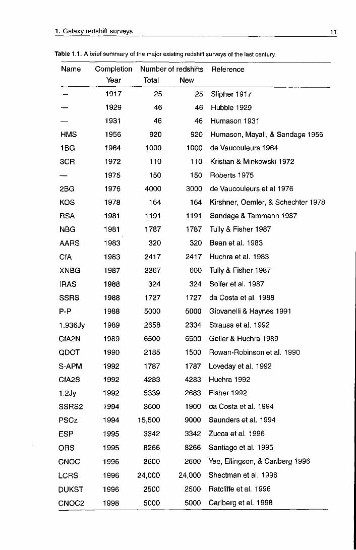
1. Ga laxy redshif t surveys 11
Table 1.1. A brief summary of the major existing redshift surveys of the last century.
Name Completion Number of redshifts Reference Year Total New
— 1917 25 25 Slipher 1917
— 1929 46 46 Hubble 1929
— 1931 46 46 Humason 1931
HMS 1956 920 920 Humason, Mayall, & Sandage 1956
1BG 1964 1000 1000 de Vaucouleurs 1964
SCR 1972 110 110 Kristian & Minkowski 1972
— 1975 150 150 Roberts 1975
2BG 1976 4000 3000 de Vaucouleurs et al 1976
KOS 1978 164 164 Kirshner, Oemler, & Schechter 1978
RSA 1981 1191 1191 Sandage & Tammann 1987
NBG 1981 1787 1787 Tully& Fisher 1987
AARS 1983 320 320 Beanetal . 1983
CfA 1983 2417 2417 Huchraetal. 1983
XNBG 1987 2367 600 Tully& Fisher 1987
IRAS 1988 324 324 Soiferetal. 1987
SSRS 1988 1727 1727 da Costa etal . 1988
P-P 1988 5000 5000 Giovanelli & Haynes 1991
1.936Jy 1989 2658 2334 Strauss etal . 1992
CfA2N 1989 6500 6500 Geller & Huchra 1989
QDOT 1990 2185 1500 Rowan-Robinson et al. 1990
S-APM 1992 1787 1787 Lovedayetal. 1992
CfA2S 1992 4283 4283 Huchra 1992
1.2Jy 1992 5339 2683 Fisher 1992
SSRS2 1994 3600 1900 da Costa etal . 1994
PSCz 1994 15,500 9000 Saunders et al. 1994
ESP 1995 3342 3342 Zucca etal . 1996
ORS 1995 8266 8266 Santiago et al. 1995
CNOC 1996 2600 2600 Yee, Ellingson, & Carlberg 1996
LCRS 1996 24,000 24,000 Shectman et al. 1996
DUKST 1996 2500 2500 Ratcliffe etal . 1996
CN0C2 1998 5000 5000 Carlberg et al. 1998

1 . Ga laxy redshif t surveys 12
"I r "I 1 r T 1 r
6
m
ra
cu
o
CU) o
1940 1960 1980 2000 y e a r
Figure 1.1: The number of known galaxy redshifts as a function of time. The dotted line represents the
results expected from future surveys.

1 . Ga laxy redshif t surveys 13
1.4 The future of redshift surveys
Recent times have seen further advances in observational capabilities. Primarily, the
development of automated techniques for fibre positioning and redshift measurement
has enabled observers to make much better use of telescope time. Efforts are directed
towards obtaining statistically large samples of galaxies, with a high degree of homo
geneity. Current surveys are much more reliable, with fewer selection problems, than
their predecessors. Deep surveys also enable the study of evolution within the sample:
both of galaxies themselves and of the way they cluster. Here we list and compare some
of the large surveys currently being undertaken or planned.
• 2dF redshift survey. The 2dF^ galaxy redshift survey (Colless 1995) being carried
out at the Anglo-Australian Telescope will measure a quarter of a million galaxies
brighter than 6j = 19.5, with a deeper extension to i? = 21 making best use of good
conditions. The brighter galaxies cover an area of 1700 square degrees selected
from both the southern galactic cap APM survey and the north galactic cap equatorial
region. In terms of clustering, the chief aim of the survey is to accurately measure
the power spectrum for wavelengths greater than 30h~^ Mpc allowing the first direct
comparison with microwave background anisotropy constraints on the same scales.
The survey's depth, particularly in its faint component, will provide measurements of
the evolution of the galaxy luminosity function, clustering amplitude, and star formation
rates out to redshifts of z ~ 0.5. The high density of observed galaxies will enable
statistically useful sub-samples to be compiled, so the variations in their clustering
properties as a function of luminosity, morphology and star formation history can all
be studied. A study of clusters and groups of galaxies in the redshift survey will also
be conducted. In particular this will examine infall in clusters and dynamical estimates
of cluster masses at large radii.
More information on the project can be found at the site
h t t p : / / m s o w w w . a n u . e d u . a u / ~ c o l l e s s / 2 d F /
• S D S S . The Sloan Digital Sky Survey (Gunn & Weinberg 1995) will measure pho
tometry for 10* galaxies in five filters. This catalogue will act as the parent for the
simultaneous redshift survey, which aims to measure redshifts for nearly a million
Two degree field, 2° being the size of the instrument field of view
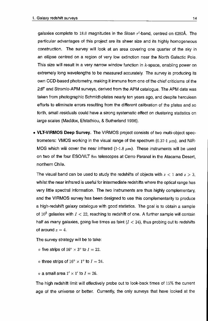
1. Ga laxy redshif t surveys 14
galaxies complete to 18.0 magnitudes in the Sloan r ' -band, centred on 6280A. The particular advantages of this project are its sheer size and its highly homogeneous construction. The survey will look at an area covering one quarter of the sky in an ellipse centred on a region of very low extinction near the North Galactic Pole. This size will result in a very narrow window function in A;-space, enabling power on extremely long wavelengths to be measured accurately. The survey is producing its own CCD-based photometry, making it immune from one of the chief criticisms of the 2dF and Stromlo-APM surveys, derived from the APM catalogue. The APM data was taken from photographic Schmidt-plates nearly ten years ago, and despite herculean efforts to eliminate errors resulting from the different calibration of the plates and so forth, small residuals could have a strong systematic effect on clustering statistics on large scales (Maddox, Efstathiou, & Sutherland 1996).
• VLT-VIRIVIOS Deep Survey. The VIRMOS project consists of two multi-object spec
trometers: VMOS working in the visual range of the spectrum (0.37-1 nm), and NIR-
MOS which will cover the near infrared (1-1.8 nm). These instruments will be used
on two of the four ESOA/LT 8m telescopes at Cerro Paranal in the Atacama Desert,
northern Chile.
The visual band can be used to study the redshifts of objects with z < I and z > 3,
whilst the near infrared is useful for intermediate redshifts where the optical range has
very little spectral information. The two instruments are thus highly complementary,
and the VIRMOS survey has been designed to use this complementarity to produce
a high-redshift galaxy catalogue with good statistics. The goal is to obtain a sample
of 10^ galaxies with I < 22, reaching to redshift of one. A further sample will contain
half as many galaxies, going five times as faint (/ < 24), thus probing out to redshifts
of around z = 4.
The survey strategy will be to take:
o five strips of 16° x 3° to / = 22.
o three strips of 16° x 1° to 7 = 24.
o a small area 1' x 1' to 7 = 26.
The high redshift limit will effectively probe out to look-back times of 15% the current
age of the universe or better. Currently the only surveys that have looked at the

1 . Ga laxy redshif t surveys 15
Universe to this sort of depth have been pencil beams, which contain very little volume,
and are thus of limited statistical usefulness. The VIRMOS project will produce de
tailed data for the study of structure evolution and the epoch of formation. The volume
probed by going to these depths will, despite the relatively small angular coverage,
result in a survey of similar size to 2dF or SDSS, and in this respect it can be regarded
as the high-redshift counterpart of these "local" surveys.
More details on the VIRMOS project can be found at the web-page
h t t p : / / l a s m O b . astrsp-mrs . f r /www_root/pro jets/virmos / V I R M O S . HTML
• 6dF Galaxy Survey. The 6dF instrument is a proposed upgrade of the FLAIR II
facility on the UK Schmidt telescope at the AAO. The proposed survey will mea
sure the redshifts of 120,000 galaxies, NIR-selected from the DENIS sky survey
(Epchtein et al. 1994) with J < 13.7, and optically selected with J > 13.7 and
B < 16.5. The survey will cover the whole of the southern galactic sky with |6| > 10°, resulting in 18,000 square degrees. Although the survey is shallower than most of
its planned contemporaries (its median redshift, z = 0.03, is similar to that of the
PSCz), its wide coverage means that it probes a large volume of the local Universe,
such that measurements will not be affected significantly by evolution in clustering or
in the galaxy population, making it an ideal calibrator for looking at evolution in the
deeper surveys. The other key advantage of this project is its use of selection in the
near-infrared. This waveband picks up the luminosity of the old stellar population,
rendering it a more direct probe of the stellar mass than the optical and far-infrared
regions, which tend to be biased towards high current star formation rates. The NIR is
also much less sensitive to dust extinction, so the survey can be used to look at galaxy
centres that would otherwise be obscured, and to go to significantly lower galactic
latitudes. At the moment no good cartography exists for |6| < 20°, and there is a lot of
solid angle in the band between that and the \b\ > 10° that 6dF will be able to achieve,
interest in this strip of sky is especially keen since it is thought the Great Attractor
lies in this obscured region, and much information about the local density field can
therefore be obtained by looking at peculiar velocities of galaxies located here. 6dF
will, then, be a useful, homogeneous sample of the local Universe. Further details are
available at the web-site
h t t p : / / m s o w w w . anu. edu. a u / ~ c o l l e s s / 6 d F /

1 . Ga laxy redshif t surveys 1 ^
• DEEP. The DEEP project (standing for Deep Extragalactic Evolutionary Probe) will conduct a survey of around 25,000 distant, faint, field galaxies, using the twin 10m Keck Telescopes and the Hubble Space Telescope (HST). The consortium of US institutions aim to use the DEIMOS spectrograph in conjunction with high resolution images from the WFPC-2 camera of HST to study evolution by looking at dynamic measures such as rotation curves and velocity widths. This should enable the study of objects containing similar mass over the range of look-back times covered by the survey The observing strategy is to select galaxies with photometry implying a redshift of between 0.7 and 1.2. Four regions of the sky will be studied, each of 120' x 15'. Each strip then will represent a volume of approximately 500 x 60 x 8h~^ Mpc^. Thus, DEEP is a powerful tool for studying galaxy formation and evolution and the origin of large-scale structure. A summary of DEEP's goals and strategies can be found in Davis & Faber 1998. The DEEP homepage address is h t t p : //www. u c o l i c k . org/~deep/home. html
Survey Solid Angle •^med Volume Number Completion sr h-^ Mpc^ Year
2dF 0.52 0.14 1.0 X 10^ 2.5 X 10^ 2001
SDSS 3.1 0.11 2.3 X lO' 1.0 X 10^ 2005
VIRMOS 0.015 1.00 2.7 X 10^ 5.0 X 10^ 2001
6dF 5.4 0.03 1.2 X 10^ 1.2 X 10^ 2002
DEEP 0.0008 1.00 1.0 X 10^ 2.5 X 10" 2002
Table 1.2. Comparison of future large galaxy redshift surveys either planned or currently acquiring data.
Table 1.2 summarizes these details, and compares the volumes probed by the different
surveys. We define the volume as one third the solid angle times the cube of the median
depth.
1.5 The need for this work
In the next ten years we will have unbiased, high density, large volume probes of the
local universe, the intermediate Universe where evolution begins to have an effect, and

1 . Ga laxy redshif t surveys 17
the high-redshift universe where we can examine the origin of galaxies and large-scale structure.
Whilst most of these surveys purport to have similar goals (ie. measuring clustering,
looking at evolution), the means of doing so is generally rather different. Once the data
arrives, it is economically expedient to make sure that it is used in the best possible way
It is likely that the best use of the data will in fact depend very much on the details of the
survey. Certain statistics will be better than others, for instance, at picking up evolutionary
effects in particular samples. Certainly, we have never dealt with data of this quality or
abundance before, and this proliferation will drive us to use new statistics that it has not
been feasible to apply to current datasets of less quality. Knowing the details of the survey
strategy in advance, though, enables us to develop new statistics and new models before
the data itself becomes available, and this is the main concern of this work.
In this thesis, then, we study a variety of different effects on the data from large sur
veys. In Chapter 2 we outline the current status of cosmological thought, the so-called
"Standard Model", and present constraints on the parameters that describe this model.
We will frequently use the power spectrum as a measure of galaxy clustering; Chapter 3
presents the fast Fourier transform method for estimating this statistic from the galaxy
distribution. Chapter 4 outlines a set of N-hody simulations that are used to produce
mock galaxy catalogues for the surveys we are interested in. These mocks have the
same angular constraints and selection functions as the real surveys, and hence are an
extremely useful testing ground for statistical analyses. One factor that can bias results
is dust extinction in the Milky Way, and we examine this effect on the power spectrum
from the SDSS in Chapter5. In Chapters we introduce redshift-space distortions to
the power spectrum as a way of extracting information about cosmological parameters.
Chapter 7 contains a detailed statistical treatment of the errors on measurements of the
power spectrum, and shows how those errors propagate through to define confidence
intervals on derived parameters. In Chapter 8 we compare the errors derived from this
technique with those found from a sample of ten independent mock catalogues. We
conclude in Chapter 9, presenting a brief summary and looking ahead to the work that
still needs to be done.

1 . Ga laxy redshif t surveys 18
References
ArpH. , 1999, A&A, 341, L5
Barrow J. D., Magueijo J., 1999, Physics Letters B, in press, astro-ph/9811072
Bean A. J., Ellis R. S., Shanks T , Efstathiou G., Peterson B. A., 1983, MNRAS, 205, 605
Carlberg R. G. et al., 1998, in Large Scale Structure in the Universe, Royal Society Discussion Meeting,
IVlarch 1998
Colless M., 1995, The 2df galaxy redshift survey, http://msowww.anu.edu.aurheron/Coiless/colless.html
da Costa L. N. et al., 1994, ApJ, 424, 1
da Costa L. N. et al., 1988, ApJ, 327, 544
Davis M., Faber S. M., 1998, astro-ph/9810489, Preprint
Epchtein N. et al., 1994, Ap&SS, 217, 3
Fisher K. B., 1992, Ph.D. thesis, AA (California Univ)
Geller M. J., Huchra J. R, 1989, Science, 246, 897
Giovanelli R., Haynes M. R, 1991, ARA&A, 29, 499
Gregory 8. A., Thompson L. A., 1978, ApJ, 222, 784
Gunn J. E., Weinberg D. H., 1995, in proceedings of the 35th Herstmonceux workshop. Cambridge Univer
sity Press, Cambridge, astro-ph/9412080
Hubble E., 1929, Proc N.A.S., 15, 168
Huchra J. E. et al., 1992, in Center for Astrophysic Redshift catalog, 1992 version.
Huchra J. E., Davis M., Latham D., Tonry J., 1983, ApJS, 52, 89
Humason M. L , 1931, ApJ, 74, 35
Humason M. L., Mayall N. U., Sandage A. R., 1956, AJ, 61 , 97
Kantor R W., 1977, Information Mechanics. Wiley New York
Kantor R W., 1999, International Journal of Theoretical Physics, accepted, astro-ph/9812444
Kirshner R. R, Oemler J., A., Schechter R L , 1978, AJ, 83, 1549
Kirshner R. R, Oemler J., A., Schechter R L , Shectman S. A., 1981, ApJ Lett, 248, L57
Kristian J., Minkowski R., 1972, in Sandage A., Sandage M., Kristian J., ed, Galaxies in the Universe.
University of Chicago press
Loveday J., Efstathiou G., Peterson B. A., Maddox 8. J., 1992, ApJ Lett, 400, L43
Maddox S. J., Efstathiou G., Sutherland W. J., 1996, MNRAS, 283,1227
Pahre M. A., Djorgovski S. G., De Carvalho R. R., 1996, ApJ Lett, 456, L79
Pound R. V , Rebka G. A., 1959, Phys. Rev Lett., 3, 439
Ratcliffe A., Shanks T , Broadbent A., Parker Q. A., Watson R G., Gates A. R, Fong R., Collins C. A., 1996,
MNRAS, 281 , L47
Rowan-Robinson M. et al., 1990, MNRAS, 247,1
Sandage A., Tammann G., 1987, in Carnegie Institution of Washington Publication, Washington: Carnegie
Institution, 1987, 2nd ed.
Santiago B. X., Strauss M. A., Lahav 0. , Davis M., Dressier A., Huchra J. R, 1995, ApJ, 446, 457
Saunders W. et al., 1994, in Proceedings of the 35th Herstmonceux workshop. Cambridge University Press,
Cambridge

1 . Ga laxy redshif t surveys 19
Shectman S. A., Landy S. D., Oemler A., Tucker D. L., Lin H., Kirshner R. P., Schechter P. L., 1996, ApJ, 470, 172
Soifer B. T , Sanders D. B., Madore B. F., Neugebauer G., Danielson G. E., Elias J. H., Lonsdale C. J., Rice
W. L , 1987, ApJ, 320, 238
Strauss M. A., Huchra J. P., Davis M., Yahil A., Fisher K. B., Tonry J., 1992, ApJ Supp, 83, 29
Tully R. B., Fisher J. R., 1987, in Cambridge: University Press, 1987
Yee H. K. 0., Ellingson E., Carlberg R. G., 1996, ApJS, 102, 269
Zucca E. et al., 1996, Astrophysics Letters and Communications, 33, 99

Chapter 2
Current status of cosmology
T H E A R G U M E N T . In order to provide the background for the rest of the work in
this thesis, we present a brief summary of the history of cosmological study to
date. We review the generally accepted cosmic paradigm from both a theoretical
and an observational viewpoint, summarizing the evidence that currently exists
to support it. We introduce the various physical properties that parameterize
this model, and describe the various constraints that recent observations have
placed on these parameters.
2.1 Introduction
This thesis is chiefly concerned with what we can hope to learn about cosmological
parameters from future galaxy redshift surveys. We will develop tools, and test them on
artificial galaxy samples, which we obtain through the use of N-body simulation. There
are a great many parameters that have an impact on the observations, even within the
context of a single broad class of models, represented by the "standard" cosmology
In order to make our objective tractable, we must restrict our analysis to certain models,
and within those models to certain ranges of parameter space. The adoption of this stan
dard cosmology then, as an effective limit on the variety of the models, reflects generally
a theoretical prejudice: many other cosmologies can and have been constructed that also
fit the available data, but they are generally felt to be even more adA70cthan the standard
model we put fonward. The standard model represents the simplest explanation of the
state of the Universe, with the fewest parameters, and is hence preferred. In contrast, the
adoption of a range of parameter space within our standard model represents observa
tional prejudice: we consider only values of the cosmological parameters that are within
the measured bounds.
2. Current s tatus of cosmo logy 21
In this chapter we first set out a brief history of our changing cosmological world view before the development of modern cosmology in the early part of the twentieth century. Following this we present a qualitative description of the standard model as it stands now. In section 2.4 we summarize the available data as it is interpreted within the framework of this model. We conclude by presenting some examples of cosmologies that fit these observations, which we will use later in our analysis.
2.2 Brief history of cosmology
Cosmology's role is to present us with a coherent World View that is in keeping with the
data available to us. Advances in cosmology have generally occurred when better data
have been available, ie. through advances in the field of instrumentation.
In the Greek world, it was generally believed that the Universe was centred on the Earth
(geocentric). Plato (427-347 BC) observed that celestial objects only moved in circles,
and the philosophers of the time drew a hard distinction between the static, unchanging
Heavens and the turbulent activity on Earth. The postulates from the time of Aristotle
(384-322 BC) survived for nearly twenty centuries with little opposition. The Greeks knew
the Earth was spherical in shape, since observers at different latitudes saw different
constellations. Hence it was natural to see the Universe as a succession of spheres.
Aristotle's cosmos used fifty-six such spheres for the planets and stars, but this simple
view couldn't explain the observations of retrograde motion of the planets that the Greeks
had made.
Aristarchus, in 290 BC, came up with the first heliocentric paradigm, with the Sun at
the centre and the Earth spinning and revolving around the Sun. Despite what now
seems to be the appealing simplicity of this view over Aristotle's multitudinous concentric
spheres, in a prevalently geocentric climate it was felt to be even less elegant, and the
idea remained undeveloped until the mediaeval renaissance.
Ptolemy (AD IOO-c.178) used Aristotle's physics of circular motions in a geocentric
framework, but offset the centres of his circles to explain retrograde motions. Planetary
positions could only be predicted to 5° accuracy, but the model lasted unchanged for well
over a millennium until the Age of Enlightenment, when intellectual freedom from religious
dogma enabled enquiring minds to address such fundamental questions. A change in

2. Current status of cosmo logy 22
perspective took place toward a heliocentric viewpoint with the work of Copernicus (1473-1543). His model had the Sun at the centre of the cosmos, with the Earth rotating on its axis and revolving around the Sun. The planets closer to the Sun move faster, and the distance to the stars is much greater than to the Sun.
Johannes Kepler (1571-1630), a student of the Danish astronomer Tycho Brahe, used
Tycho's extremely precise data on Mars' retrograde motion to develop a physical realiza
tion of the Copernican model. He showed that Mars has an elliptical, rather than circular,
orbit around the Sun, and went on to formulate his three laws of planetary motion, later
incorporated by Newton into his theories of forces and gravity.
With a working view of our own solar system, it became interesting to study the nature
of the stars, known since Ptolemy's time to lie at much greater distances than the planets.
In the late eighteenth century William Herschel developed the idea of using star counts
to determine the shape of the stellar distribution. Assuming that stellar luminosities do
not evolve with their distance away from us, but the only effect of distance is to dim
their apparent magnitudes according to the inverse square law, counting the number
of stars in each direction down to a certain magnitude limit produces a map of the
spatial distribution of the stars. Well into the beginning of our century the special place
of the Earth in the Universe was still an accepted view point, backed up by Kapetyn's
confirmation of Herschel's result that the Earth was at the centre of an "Island Universe".
As will be discussed in Chapter 5, this was a result of dust obscuration dimming the
starlight in excess of the inverse square law, preventing the number count technique from
probing significant scales, and making deduced stellar distances much larger than their
true values. Figure 2.1 shows a comparison of Kapetyn's Universe with the picture we
currently have of the Milky Way drawn to the same scale.
Kapetyn's Universe
40,000 light years
The Milky Way
Figure 2.1: Kapetyn's view of the Galaxy, and our present understanding. Forty thousand light years Is
roughly 13kpc.
2. Current status of cosmology 23
Some key factors in modern cosmology were foreseen by Immanuel Kant in his 1755 opus "A universal natural fiistory and tlieory of the lieavens". Kant suggested tliat tlie observed nebulae miglit be similar to our own Milky Way, but external to it. He was also the first to suggest that structures could grow via gravitational instability from tiny random perturbations in an initial density field. Despite Kant's prescience, modern cosmology would have to wait for more than a century until observational techniques enabled astronomers to break free of our own Galaxy. Pioneering work was done by Shapley in measuring the true shape of our Galaxy using Cepheid variable stars in globular clusters around the Milky Way as distance indicators. Shapley, however, was adamant that the spiral nebulae were small objects associated with our galaxy, and this stance provoked the Great Debate of the 1920's between Shapley and Curtis, who put fonward Kant's hypothesis that they were distant copies of the Milky Way. The observation of high recession velocities resolved the debate in Curtis' favour. Modern observational cosmology thus began, with the final blow to the anthropocentric view that mans position in the Universe is somehow "special".
2.3 The standard cosmological model
The linchpin of modern cosmological thought is the the Copernican Principle, which
states that our vantage point should not be at any preferred location in the Universe.
Thus, all observers should measure a Universe that is the same in a statistical sense. The
acceptance of this principle leads us to consider the concepts of /sofropy and homogene
ity. Isotropy is the invariance of the observed Universe when the observer undergoes a
rotational transformation, and homogeneity is invariance under a translational transform.
It is by no means obvious that the Universe should have such symmetries, and in no
way does either symmetry, taken on its own, imply the other: an homogeneous universe
could be anisotropic, if the anisotropy were in the same direction for all observers; and
an isotropic universe could consist of concentric shells around the observer of varying
density, hence being inhomogeneous.
An extension of the Copernican Principle is the Cosmological Principle, which states
that the Universe must be homogeneous and isotropic. Isotropy can be measured
using either number counts of distant galaxies or the cosmic microwave background.
Homogeneity can be tested using the information from large redshift surveys to see

2. Current status of cosmology 24
if the Universe looks the same to a distant observer as it does to us. If the CMB
really is cosmological in origin, its high level of isotropy is a powerful argument for the
Cosmological Principle. Direct evidence for homogeneity is, on the other hand, rather
weak at the moment, although the forthcoming large redshift surveys should be able to
probe the scales at which we expect to see the turnover to homogeneity in the galaxy
distribution.
The observation that galaxies are moving away from each other provokes the highly
pertinent question, what would we see if we reversed time's arrow and watched the
Universe contract? Thanks to the finite speed of light, this is not an abstract question
but is, up to a point where the density is such that the Universe is opaque to this light,
eminently answerable. Going back further than this barrier, we are in the realms of
speculation, but not w/Zaf speculation; if the laws of physics appear to apply all the way to
the edge of the boundary, we are justified in extrapolating them back even further. This
extrapolation must eventually break down; we have only tested our laws of physics in
the laboratory up to certain finite extremes of temperature and density. Beyond these
extremes we apply imagination, and a supposed feeling for "elegant solutions". But the
onus isn't on the Universe to behave elegantly according to our concepts, as Aristotle
would realize if he could see the state of the subject today The onus is on us to push
forward our understanding by experiment and observation.
2.3.1 Geometry of spacetime
In order to describe the topology of the expanding Universe, we employ the formalism
of General Relativity. Unlike the Galilean or Special relativistic coordinate transforms
employed in section 1.2, the transform of GR is curved, in the sense that it has a spatial
dependence which is a function of the mass distribution. The transform is described by
Einstein's field equations, and all cosmological models are solutions of these equations.
Although the equations can be presented neatly using tensor calculus, in their general
form the are difficult to solve, involving many dimensions. The adoption of the Cosmolog
ical Principle introduces several symmetries that make the equations far more tractable.
De Sitter solved Einstein's equations for the simplest case in 1917, but for this Universe
to be static it can contain no matter - othenwise it will expand. It was this apparent
paradox, before the expansion of the Universe was observed, that prompted Einstein
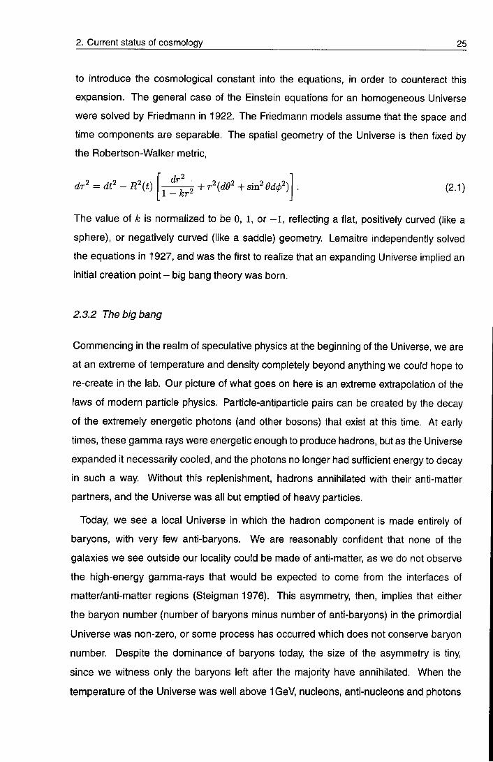
2. Current status of cosmology 25
to introduce the cosmological constant into the equations, in order to counteract this expansion. The general case of the Einstein equations for an homogeneous Universe were solved by Friedmann in 1922. The Friedmann models assume that the space and time components are separable. The spatial geometry of the Universe is then fixed by the Robertson-Walker metric.
Wr2 + r\de'' + s\r?edct?)
1 - A ; r 2 (2.1)
The value of k is normalized to be 0, 1, or - 1 , reflecting a flat, positively curved (like a
sphere), or negatively curved (like a saddle) geometry. Lemaitre independently solved
the equations in 1927, and was the first to realize that an expanding Universe implied an
initial creation point - big bang theory was born.
2.3.2 The big bang
Commencing in the realm of speculative physics at the beginning of the Universe, we are
at an extreme of temperature and density completely beyond anything we could hope to
re-create in the lab. Our picture of what goes on here is an extreme extrapolation of the
laws of modern particle physics. Particle-antiparticle pairs can be created by the decay
of the extremely energetic photons (and other bosons) that exist at this time. At early
times, these gamma rays were energetic enough to produce hadrons, but as the Universe
expanded it necessarily cooled, and the photons no longer had sufficient energy to decay
in such a way. Without this replenishment, hadrons annihilated with their anti-matter
partners, and the Universe was all but emptied of heavy particles.
Today, we see a local Universe in which the hadron component is made entirely of
baryons, with very few anti-baryons. We are reasonably confident that none of the
galaxies we see outside our locality could be made of anti-matter, as we do not observe
the high-energy gamma-rays that would be expected to come from the interfaces of
matter/anti-matter regions (Steigman 1976). This asymmetry, then, implies that either
the baryon number (number of baryons minus number of anti-baryons) in the primordial
Universe was non-zero, or some process has occurred which does not conserve baryon
number. Despite the dominance of baryons today, the size of the asymmetry is tiny,
since we witness only the baryons left after the majority have annihilated. When the
temperature of the Universe was well above 1GeV, nucieons, anti-nucleons and photons
2. Current status of cosmology 26
would have had approximately the same abundances. If we thus attribute one third the number of photons we see today to primordial abundance, and two-thirds to the reaction
b + b - ^ j + -f, (2.2)
we see that the primordial excess of matter over antimatter is given by:
ns ~ O + nO /3 " I + ^ ^ b / S ' (2-3)
where the superscript zero refers to current abundance. A measurement of the baryon-
to-photon ratio comes from big bang nucleosynthesis theory, which will be discussed in
section 2.4.6. Independent, but weaker, constraints come from comparing the baryonic
component of galaxy clusters to the density of photons in the cosmic microwave back
ground. The tiny value of r/ obtained from these techniques implies an original asymmetry
of order one part in one billion.
The next phase of creation is the lepton era. Below the GeV level needed to produce
hadrons, the photons can still produce electron-positron pairs. In this bath of leptons, the
neutron and proton populations are kept in equilibrium since ;9-decay is balanced by the
inverse process, positron capture by neutrons. This balance continues until the photon
temperature drops below the MeV level needed for pair production, and neutrons can
only decay. The neutron takes centre stage for its fifteen minutes of fame, for its mean life
is just a quarter of an hour. Neutrons and protons can combine to produce the deuteron;
these deuterons can then combine with another neutron to produce the third isotope of
hydrogen, tritium. The final capture of another proton promotes our particles to Helium
nuclei. Lithium and Boron can also be produced at this time. This process is called
nucleosynthesis for obvious reasons. In a matter of hours there are no more unbound
neutrons left in the Universe, and the abundances of the elements are frozen until such
time as fusion processes in stars can alter them.
Matter and radiation were in equilibrium while photon energy was large, but now there
is very little mass left, and the radiation dominates the energy content of this primordial
fireball. The radiation pressure continues to drive the expansion, but since photons are
relativistic particles, their energy goes as the fourth power of the scale factor. As the
Universe cools, the matter component becomes non-relativistic and its energy density
will decrease as the cube of the scale factor. So, no matter what the amplitudes of

2. Current status of cosmology 27
these functions, there must come an era when the energy density is matter-dominated.
Radiation and matter are still in good thermal contact, though, due to Compton scattering
of photons off all the free electrons, so the two populations have a common temperature.
This picture is changed at recombination: the temperature drops below 13.6eV, the ion
ization temperature for Hydrogen, and the electrons can theoretically settle down into the
shells of the hydrogen nuclei to produce atoms. This does not occur, in fact, until rather
lower temperatures have been reached, since the radiation has an energy spectrum with
a Planck distribution and photons in the high energy tail can still dissociate the atoms.
The ratio of photons to baryons is so high (77 ~ 10^) that this continues to be significant
at much lower energies. Bound electrons are much less efficient scatterers of light than
free ones due to the restrictions on the wavelength of light they can absorb imposed on
them by quantum mechanics. Thus the Universe rapidly changes from being opaque to
light to being practically transparent. The photons are decoupled from the mass and the
two components now follow separate thermal histories.
2.3.5 Structure
There is one obvious problem with the standard model of a homogeneous spacetime: it
fails to provide a mechanism for the creation of the wealth of structure that we see around
us in the Universe today, and indeed for our own existence.
Observations of the microwave background have revealed the presence of small fluc
tuations in this photon field. This is the only observable sign of structure other than that
seen by surveys of the present-day Universe. To develop a theory of structure formation
requires speculation to interpolate between these two epochs, and to extrapolate back
before the surface of last scattering to explain the primordial nature of these fluctuations.
Starting in the beginning, we turn to the quantum world for an explanation. As the
early Universe expanded, tiny but unavoidable perturbations in it caused by quantum
fluctuations would also expand. These fluctuations would be Gaussian distributed with
amplitude given by the Harrison-Zel'dovich power spectrum, P{k) a where n is unity
(ZeI'dovich 1972). This model is preferred because it is scale-invariant. As the Universe
expands, the volume of space in causal contact with the observer increases. This volume
is known as the observer's horizon, and for a scale-invariant power spectrum all the

2. Current status of cosmology 28
modes have the same amplitude at the time they come inside this horizon, and there is no physical scale introduced other than that of the horizon itself.
Outside the horizon, in the radiation dominated era, the modes all grow with the square
of the expansion factor, d{t) oc a{t)'^. The power spectrum goes as the linear growth
factor squared, P{k,t) cx d{t)'^. Once the perturbations come within the horizon, they
are decoupled from the expansion of the Universe and cease to grow. This behaviour
stops at matter domination, when the growth factor behaves linearly with the expansion
factor for modes both inside and outside the horizon, effectively maintaining the shape of
the fluctuation spectrum. Thus we expect to see today the Harrison-Zel'dovich spectrum,
P{k) oc k, on the largest scales, with P{k) cx k'^ on small scales. The position of the
turn-over between the two asymptotes provides useful information on the horizon size at
recombination.
The fluctuations of the CMB are thus the signature of perturbations in the mass field,
stamped on to the photon field at the time of decoupling.
After recombination, gravitational collapse means that areas with positive fluctuation
attract more matter and become denser, whereas areas of negative fluctuation are grad
ually emptied of matter. The mathematics of linear evolution of the density modes is set
out in Appendix A. Linear evolution is strictly only valid in the regime where the fields in
question have amplitude much less than unity. Beyond this linear level the Press-Schecter
formalism (Press & Schechter 1974) is often used to trace the evolution of the objects that
will become galaxy haloes. This treatment assumes that, although the density field may
be non-linear, the amount of matter going in the central, virialized halo is the same as that
initially contained in its Lagrangian radius, and this flow is independent of the distribution
of the mass within this radius. Alternatively this regime is modelled using the method of
computational A/-body simulations.
2.3.4 Inflation
The inflationary paradigm is invoked to answer several key questions raised by the stan
dard model, including:

2. Current status of cosmology 29
• Isotropy. The size of the horizon at recombination was, when projected onto the sky,
~ r. How come the CMB is isotropic over much larger scales than the causality scale
when it was formed?
• Anisotropy. Below the horizon scale, what caused the tiny anisotropies observed in
the CMB that later seeded the formation of structure?
• Flatness. The Universe today is very close to flat. What a priori reason is there for
the curvature to be less than or comparable to the energy density of matter?
Inflation models the vacuum energy of the Universe as the potential of a scalar field, cj).
It is assumed that there is a spontaneous symmetry breaking transition in this field at a
certain energy scale, Tc. At temperatures greater than this, 0 is a symmetrical field with a
minimum at the origin, ^ = 0. As the Universe cools, it eventually reaches temperatures
comparable to Tc and the symmetry is broken; a secondary minimum in the potential
comes about, say at = a. As the Universe continues to cool, this minimum becomes
the global minimum potential for the field. The passage of the field from 0 = 0 to = CT is
what drives inflation. This behaviour is illustrated in figure 2.2.
v(^)
Figure 2.2: The behviour of the scalar field, V{(1>), at three different temperature regimes, as discussed in
section 2.3.4.

2. Current status of cosmology 30
Firstly quantum or thermal fluctuations allow 4> to tunnel through the potential barrier separating it from the next "valley". Providing the potential is sufficiently shallow, the Lagrangian for 4> is then dominated by a friction-like term, and this "slow-roll" inflation drives an exponential increase in the expansion factor of the Universe. After the slow-rolling era, 4> proceeds to oscillate about its minimum, losing energy through particle production as it converges on ^ = <t . This energy re-heats the Universe to the temperature it was at before the exponential expansion took place. This model, then, resolves the shortcomings of the standard model mentioned above. The homogeneity problem is solved because, before inflation, the currently observable Universe was contained in a causally linked patch. Anisotropies are the result of inflation-amplified quantum fluctuations in the field, (f). The Universe after after inflation is necessarily very close to flat since the energy density has effectively remained the same, but the Universe has expanded enormously wiping out the curvature component. For a more detailed introduction to inflation, see Kolb& Turner (1990), §8.
2.4 Observational evidence
What observational evidence is there for the Standard Model? What are its failings? And
to what extent do we know the values of the parameters in the model? The parameters
have left their signatures on the Universe in a number of different ways. None of them
can be measured directly and all require detailed physical models to relate them to
observable quantities.
2.4.1 Expansion
As outlined in Chapter 1, Nubble's Law for relating galaxy redshifts to their distances from
us is a key tool with which to examine cosmological models. There are several "standard
candle" techniques for measuring the value of the Hubble constant, HQ, but large un
certainties in the calibration for most of these methods. This uncertainty leads to a wide
variety in the measured value, though most groups find 40 < ffo < 100km M p c " \ with
many recent determinations seeming to converge on a value o f « 65kras~^ Mpc~^ Apart
from the normalization of the relation, the existence of a linear dependence of distance on
redshift for close objects has been proved beyond doubt, and this result is a cornerstone

2. Current status of cosmology 31
of the standard model. Many techniques are prone to systematic bias since they rely on calibrating distant standard candles at medium redshifts using other standard candle techniques that have been calibrated locally Thus we have a picture of a cosmological "distance ladder", where higher redshift techniques stand on the shoulders of more local measurements.
Non-linear deviations from the relation, parameterized by a second order expansion of
the relation such that
z = HodL + ^{qo-l){HodLf, (2.4)
are probes of spatial curvature. Current constraints on go are very weak, since the signal
at high redshift, where we would expect to see the departure from linearity, is contami
nated by the possible evolution of the objects we are looking at with look-back time. The
most sensitive current probe of this quantity is the flux from high-redshift supernovae,
outlined in section 2.4.7. Certain techniques, eg. the Sunyaev-Zel'dovich effect which will
be discussed in section 2.4.5, are capable of directly measuring the expansion rate over
large distances, but at present the errors are large.
2.4.2 Age
Measurements of the age of the Universe can be directly tied into constraints on the
cosmology and the value of HQ. The age is given by:
Hoto = dy
y 2 [ l + O o ( y - l ) - A o ( l - l / 2 / 2 ) ] i / 2 (2-^)
where y = I + z. It can be seen that for the simple Einstein-de Sitter model with no
curvature or cosmological constant, this equation results in simple expression HQIQ =
2/3.
Measurements of the age of the Universe itself cannot be made independently of the
cosmological framework, but this is not true for measurements of the objects within the
Universe. It is generally considered reasonable to assume that the Universe must be
older than the age of any objects in it. An immediate constraint on the age of the Universe
can, then, be made on purely terrestrial grounds: by examining radioactivity in rocks,
which decays with a known lifetime. For a variety of different isotope ratios, the results are

2. Current status of cosmology 32
consistent with an age of the Earth of around 4Gyr. This result is confirmed by estimates
of the age of the Solar System from isotope ratios in meteorites. The standard value
for the age is now around 4.6 ± O.lGyr (Wasserburg et al. 1977). Using the observed
abundances of heavy elements, an age limit of between 7 and 13Gyr is found for material
in our galactic disk, depending on how these elements formed. Stellar evolution models
predict 16 ± 2Gyr for the oldest globular clusters in the galactic halo, (Renzini et al. 1996),
although some more recent determinations point to rather lower results of a maximum
age of 14Gyr (Salahs, Degl'lnnocenti, & Weiss 1997; Jimenez & Padoan 1998). To relate
these ages to bounds on Nubble's constant or the cosmological model, we note that the
units of Nubble's constant are kms"^ M p c - ^ It so happens that this unit is almost exactly
one inverse terayear, so the relationship between time and Nubble's constant is simple if
0 is expressed in units of lO^^yr. For an Einstein-de Sitter model, then, to = 16± 2Gyr
implies a Hubble constant of 2/(3 x 0.016) = 4 2 ± 5 k m s ~ ^ Mpc"^ This result would seem
in disagreement with the observed value mentioned in the section 2.4.1, so the simple
Einstein-de Sitter model is excluded by this data.
2.4.3 Microwave background
The Cosmic microwave background (CMB) is, paradoxically one of the most powerful
arguments for isotropy and homogeneity in the Universe and simultaneously one of the
most informative tools for examining the precise details of the anisotropies that we believe
have led to the formation of the structure we see around us.
• Homogeneity. The CMB was discovered accidentally by Penzias and Wilson in 1965,
as they were measuring microwave emission from our own galaxy and observed an
isotropic source of detector noise in their radio antenna. This noise appeared to be at a
temperature of around 4K, and did not change with direction, within the limited angular
resolution of the experiment. The theoretical framework of a microwave background
had been laid down a decade earlier by Gamow, who showed it to be a natural
prediction of an expanding, cooling Universe. Once its significance was realized (by
Dicke), a number of experiments set out to measure the temperature accurately and
look for deviations from isotropy A primary anisotropy was observed a decade later
(Smoot, Gorenstein, & Muller 1977), a dipole term that is interpreted as representing

2. Current status of cosmology 33
our motion with respect to a cosmic reference frame. Beyond this dipole, though, the CMB is smooth to a level of one part in a thousand.
No non-cosmological model is capable of producing the degree of isotropy observed
in the CMB, and its observation is one of the cornerstones of the standard cosmology
Simultaneously it is one of the models biggest deficiencies. In an expanding universe
with a finite speed of light, objects can only be in causal contact if they are in within
each other's particle horizon, the furthest distance a photon from one of the galaxies
could have travelled if it set out at the moment of creation. If the CMB really is radiation
left over from recombination, the particle horizon then was small compared to the
distance between pockets of space that are observed in different directions by us now;
only areas of separation ~ 1° could have been in contact at or before the formation
of the CMB. If areas are not in causal contact, it is difficult to see why they should
have the same properties, so the high level of isotropy is one of the chief failings of the
standard model. This problem can be overcome, as mentioned earlier, by expanding
the standard model to include inflation (section 2.3.4).
• Anisotropies. Anisotropy beyond the dipole term was first observed by the COBE
satellite in the early 1990's (Smoot et al. 1992). This result has become a key tool in
the understanding of cosmology and structure formation, since it is believed that the
fluctuations observed in the radiation reflect the seeds that would grow into observable
structure in the matter distribution.
There are three primary sources of anisotropy:
o Gravity. The gravitational field caused by an overdensity redshifts a photon climb
ing out of it.
o Doppler Matter with a peculiar velocity will Doppler shift the photons it scatters
according to its direction.
o Temperature. Denser matter is hotter, so photons from overdense areas are more
energetic.
On the largest scales, the kinetic energy effect is related linearly to the gravitational
field. This results in a scale-independent fluctuation spectrum, known as the Sachs-
Wolfe effect. The other effect that can be considered a primary one is the finite
thickness of the last scattering surface (LSS). Anisotropies on scales smaller than this

2. Current status of cosmology 34
thickness are washed out by the radial smoothing that is applied implicitly when data
are averaged from a range of look-back times. These two very simple considerations
(Sachs-Wolfe at large scales and finite thickness on small scales) are responsible
for the asymptotic behaviour of the angular power spectrum, as demonstrated by the
model spectrum (solid line) in the upper panel of figure 2.3.
On intermediate scales, the photon-baryon fluid undergoes damped oscillations. As
perturbations enter the horizon, they all start with the same initial conditions, ie. the
same phase. In the adiabatic case this corresponds to 5 = 0, 5 = -2(^: like a
pendulum at the top of its swing, it has all potential, and no kinetic, energy The
CMB we observe is a "cosmic snapshot' of these perturbations at a fixed time, at
which shorter wavelength modes have been inside the horizon longer than large-scale
perturbations, and hence have a more advanced phase. This leads to the nearly
periodic behaviour in k seen in figure 2.3.
The amplitude of the oscillations depends on how tightly the photon field is coupled
to the underlying mass distribution. The photons only interact with the baryonic
component, so the peaks are higher in a model with a higher baryon fraction. The
amplitude of CMB anisotropies is thus a useful probe of Q^-
The location of the peaks, in contrast, measures the geometry of the Universe. The
power spectrum of the fluctuations has a fixed physical scale, but when observed in
projection, the translation to /-space depends on geometry:
2r (a = 0.4 for a flat model I = r]k, where r? = -r-J^o ° { (2-6)
-no [ a = 1.0 for an open cosmology
Measuring k in units of / i M p c " \ this becomes r) = 6OOOO0" ^
After recombination, the photon field is only coupled to the mass field via gravitational
effects. In the time-independent case, if a photon travels into a potential well, the blue
shift it gets is exactly cancelled out by the redshift it picks up as it climbs out again.
However, if the potential evolves as the photon is travelling through it, this is not the
case, and the photon may obtain a net blue or redshift. This effect is known as the
integrated Sachs-Wolfe (ISW) effect, and there are three different ways in which the
potential become time-dependent:
^ 6000A ^ Mpc is the comoving distance corresponding to the redshift of the epoch of recombination.

2. Current status of cosmology 35
o Early ISW. At z = ZREC, the photon density is small but non-negligible, and as matter starts to dominate the energy density, its importance fades away, resulting in an evolving potential.
o Late ISW. Depending on the cosmology at late times the Universe may become
vacuum or curvature dominated. In this case, the potential will again become time-
dependent.
o Rees-Sciama. At moderate redshifts, non-linear structures start to form, structures
which evolve at a significant rate compared to the time taken for photons to cross
them. Thus the potential a photon undergoes on climbing out of the potential well
need not be the same as it experienced on the way in.
These effects also leave their mark on the CMB we observe today Although they
tell us little about the primordial density fluctuations themselves, they can act as
useful cosmoiogical probes in there own right. In general they result in only mild
perturbations to the primary anisotropies; the late ISW affects only the largest scales,
the early ISW affects only the first Doppler peak, and the Rees-Sciama effect has
a negligible effect on the power spectrum for cold dark matter models of structure
formation (Tegmark 1996).
Another gravitational effect that is thought to be of importance in the CMB signal is that
of weak lensing of photons by structures close to the line of sight between emission
and the observer. This effect leads to a smearing of the power spectrum since photons
appearing to come from a certain patch of sky can, in reality, have originated from
a wider area. A similar smoothing can be caused by a global reionization of the
Universe. In this case, photons can Thomson scatter off a more recent surface than
that at recombination, and information about their original points of origin is lost.
COBE gives us constraints on large-scale anisotropy, where the angular power spec
trum has no features. The four-year COBE data is plotted in figure 2.4. It is readily
apparent that the chief contribution to the anisotropy is the dipole caused by the Earth's
motion relative to the CMB frame. Once this dipole is removed from the signal, the
primordial anisotropies are clearly visible. The middle panel of this figure is still con
taminated by emission from the Milky Way seen as the strip across the middle of the
projection. The corrected data can be used, given a particular cosmology to predict
the shape of the power spectrum. Further experiments have measured fluctuations on

2. Current status of cosmology 36
CAT >t2 <
MSAM ARGO COBE
I I I I I 1 I 1000
50
40
Anisotropy detections c. 1997
A
V
30
20
10
1 1 1—I I I I I I 1 1 1 I i I I I I 1 1 1 I M I I
I I I I I I I _] I I I I I
10 100 1000
Figure 2.3: Plots of the multlpole power spectrum, Ci, using results from various CMB experiments. The
lower plot reflects the bounds obtained by averaging the individual experiments presented in the upper plot.
Source: http://www.astro.ubc.ca/people/scott/q-values-97.html

2. Current status of cosmology 37
Figure 2.4: The microwave background from COBE. The upper panel shows the from the four year, uncor
rected data in the 53GHz channel. The middle panel dhows the result of subtracting off the dipole. The
lower panel shows the result of subtracting a model of the Galactic emission and masl<ing out areas of high
contamination. Source: http: //www. gsf c.nasa. gov/astro/cobe/dmr.image.html

2. Current status of cosmology 38
much smaller scales, either from ground-based or airborne experiments. At present, the consensus of opinion is that the existence of the first Doppler peak is fairly well established, but current measurements are not good enough to fix the peak or its amplitude. In figure 2.3 we show the current state of CMB observations as presented by Scott (1997). The averaged plot shows the Doppler peak quite clearly putting it somewhere in the range / - 200-500.
Planned CMB experiments such as MAP ^ and Planck (Lawrence & Lange 1997) will
be able to measure the CMB with far greater accuracy than any existing equipment,
resulting in a wealth of data with which to constrain the cosmological parameters.
Detailed studies of CMB polarization as well as temperature maps aim to break some
of the inevitable degeneracy in fitting complex models to a single curve.
2.4.4 Galaxy surveys
The progress of three-dimensional redshift surveys has been described in Chapter 1.
Redshift surveys have generally been confined to examining rather small volumes of
space and this restriction has limited their use in looking at the linear part of the power
spectrum, which is where much of the cosmological information is contained. Angular
surveys can probe much larger volumes of space with good sampling rates, given the
relative ease of measuring the position of an object on the sky rather than measuring its
spectrum accurately enough to obtain a redshift. There is, of course, no information in an
angular survey about the redshifts of the galaxies, but this problem can be circumvented
given a redshift distribution in a statistical sense. Baugh & Efstathiou (1993 and 1994)
show how the angular correlation function or power spectrum of galaxies in the APM
Galaxy survey (Maddox et al. 1990) can be inverted, given a model for the distribution of
galaxies with redshift, to produce the full three-dimensional power spectrum. This model
is seen to be fairly robust to changes in the assumed galaxy distribution, and provides
the most accurate currently available view of clustering on the largest scales, although
there are uncertainties in tracing the power spectrum over the 'bump'; the APM survey
is based on 6° x 6° plates, and possible mismatches in the calibration of adjacent plates
means the angular correlation function is prey to systematics on these scales, which is
the region of interest as regards spotting a turnover in the power spectrum. Dust is also
http://map.gsf c.nasa.gov/

2. Current status of cosmology 39
a contaminant affect ing the correlat ion function (Schlegel, Finkbeiner, & Davis 1998), an issue we will explore in greater depth in chapter 5. The quoted random errors, as well, are open to crit icism, since they come from the simple technique of splitting the survey into four patches and measur ing the variance between these parts of the sl<y. They are thus likely to be a ser ious underest imate of the true error, particularly on the largest scales, for wh ich the ampl i tudes in adjacent patches will be highly correlated. Results from the APiVl survey point to a value of crf^' (the variation in galaxy number counts in spheres of radius 8h~'^ Mpc) of between 0.84 and 0.96. The conversion of angular data to constraints on the three-dimensional power spectrum is sensitive to assumptions about the evolution of c luster ing and cosmology, and hence this range of values represents the systematic uncertainty (Baugh, private communicat ion). The power spectrum is assumed to evolve as
P{k,z)=P{k)/{l + z f + ' - \ (2.7)
where 7 w 1.7 is the slope of the correlation function, and e parameterizes the
clustering evolut ion. For e = 0, small scale clustering is fixed in physical co
ordinates, and the ampl i tude of the A P M power spectrum is o-g = 0.96 ± 0.04
(Maddox, Efstathiou, & Suther land 1996). Redshift surveys have been employed to cor
roborate these values: the Stromlo-APM survey (Loveday et al. 1996) finds as = 0.89 ±
0.05. If the shape of the power spectrum is parameterised by a CDM-like transfer function
(Efstathiou, Bond, & Whi te 1992), the value of r derived from the APM data is found to
be 0.2-0.3. (Baugh & Efstathiou 1994; Maddox, Efstathiou, & Sutherland 1996). The
relatively large error here reflects the uncertainty of the location of the turn-over and the
large error-bars on points at small k. The CDM spectral shape is in fact not a good match
to the A P M data, if the errors can be trusted. In fact, the APM errors are calculated
by looking at the variance in est imates from four adjacent quadrants. Especially on
large scales, these measures will be correlated, and the A P M errors are likely to be
an underest imate of the true uncertainty. The poor quality of the fit is responsible in part
for the variety of values for the est imated r.
Redshif t surveys can also be used to constrain the /3-parameter ( « where b is
the b ias parameter, the ratio of galaxy overdensity to the underlying mass overdensity).
The galaxy power spectrum is distorted in redshift-space by the peculiar velocities of the
galaxies, wh ich depend on the density. (3 can be measured internally, by comparing the

2. Current status of cosmology 40
quadrupole- to-monopole ratio of the distorted clustering, or by lool<ing at t l ie boost in the monopo le power relative to the power spectrum of the parent angular catalogue. This latter technique has been used in the Stromlo-APM redshift survey (Loveday et al. 1996). Values for /? range between 0.5 and 1 depending on the way the galaxies are selected. Some sample dependence is expected since different types of galaxies are expected to have different clustering propert ies, and different values of the bias and hence (5. Current measurements are reviewed in Hamilton 1997. Dekel (1998) shows how a stochastic, non-l inear model for bias can account for some of the scatter in estimates of /3 made using different techniques.
2 .4 .5 Clusters
Clusters of galaxies are the largest virialized systems in the Universe, and as such
are a ferti le hunt ing ground for information about structure on scales approaching the
l inear regime where cosmological parameters play an important role. Constraints from
cluster measurements are not sensitive to the details of galaxy formation, making them
a powerful and robust tool. There have been two chief methods using clusters to probe
cosmology:
• A b u n d a n c e . The Press-Schechter formalism (Press & Schechter 1974;
B o n d e t a l . 1991) can be used to predict the abundance of objects of a given
mass if structure is caused by initial f luctuations with Gaussian random phases.
Several authors (White, Efstathiou, & Frenk 1993; Eke, Cole, & Frenk 1996) have
employed this method to constrain cosmology. The mass function thus derived is
converted to a temperature function under the assumption that the gas is isothermal.
Eke, Cole, & Frenk (1996) use the simulations we outline in Chapter 4 to assess the
accuracy of the Press-Schecter results, and in general good agreement is found. This
agreement is part icularly good at the high-mass end, but the P-S treatment is known
to disagree with simulations in the low-mass regime. In order to constrain cosmology,
a compar ison is made to the local abundance of clusters as a function of their X-ray
temperature. That work uses a sample of twenty-five low redshift clusters compiled
by Henry & Arnaud (1991). The best current results have
(a = - 0 .46 + O.lOOo for open cosmologies as = (0.52 ± OM)n^ I (2.8)
[ a =-0.52 + 0.130.0 for flat models.

2. Current status of cosmology 41
These results are found to be quite insensitive to the shape of the power spectrum, so
provide a .direct and independent constraint on o-g for a given cosmology.
• Evolut ion. Having normal ized the local cluster abundance, looking for evolution with
redshift can be a powerful tool. The basic theorem used here is that, in models with
low fio. the Universe has not changed much in recent t imes: the rapid expansion of the
Universe, caused by having a low energy density, acts to prohibit any further growth
of structure, and evolution is suppressed relative to a model with fio = 1- Adding
a cosmological constant term causes structure to be frozen out at lower redshifts,
producing slightly stronger evolution in a flat cosmology as opposed to an open one.
In particular, the X-ray temperature of gas in a cluster is, by the virial theorem, a
funct ion of the mass of the cluster. This enables constraints to be placed on the
value of UQ. It has been shown by Kay & Bower (1998) that X-ray luminosity evolution
a lone cannot constrain Oo> but that measurements are degenerate with the slope of
the power spectrum on cluster scales. An independent measure of this local slope is
thus needed to produce a good constraint. They conclude < 0 . 7 5 using such a
measurement . Eke et al. (1998) derive a constraint of OQ = 0 . 4 5 ± 0 . 2 5 by examining
the behaviour of the X-ray temperature function with redshift.
A further technique involving cluster evolution is to look for the Sunyaev-Zel'dovich
effect (Sunyaev & Zel 'dovich 1972). CMS photons are scattered upwards in energy
by coll isions within a cluster with the hot electron plasma. The net effect is to produce
a bump in the C M B spectrum along the line of sight to the cluster; photons are taken
out of the distribution at one energy, and scattered out of the line of sight or into the
line of sight but at a higher energy, causing a decrement at long wavelengths. The
extent of this effect depends on the temperature of the electron gas, making it a useful
probe of evolut ion.
All current work on cluster evolution has a high level of uncertainty due to the lack of
a large sample of wel l -measured clusters at high redshift, but will be a powerful tool
when better data become available.

2. Current status of cosmology 42
2.4.6 Big-bang nucleosynthesis (BBNS)
As already d iscussed, BBNS occurs during the epoch after the Universe has cooled
sufficiently that it cannot pair-produce electrons and positrons. The light elements,
deuter ium, hel ium and lithium are produced. Today, deuter ium abundance is measured
a long lines of sight through the interstellar medium. Deuter ium has a very low binding
energy, making it hard to produce in any astrophysical environment. Thus the ratio today
should be a lower limit on the BBNS ratio. Most deuter ium depletion occurs in stars,
which general ly convert the isotope to ^He. We can estimate the difference between the
pre-solar and processed ^He abundance by comparing its concentration in dust on the
Moon's surface with the nearly primordial amount found in the primitive meteorites known
as carbonaceous chondri tes. Assuming the difference to come from solar processing of
deuter ium al lows us to measure the deuter ium depletion and hence the total primordial
abundance.
Hel ium is produced in stars, but not nearly enough to explain the ~ 1:10 ratio of ^He to
hydrogen. The '*He abundance is a crucial test for the big bang model of cosmogony itself,
but is in fact insensit ive to cosmology. Observed in H i i regions via its recombination line,
the ratio appears to be universal. The abundance of deuter ium, however, does depend
on cosmology. Deuter ium can be destroyed by proton collisions, and in a less dense
universe, there is less chance of such collisions, so deuter ium is preserved.
Walker et al . (1991) present a thorough examination of BBNS using recent data for the
nuclear reaction cross sections, the half-life of the neutron, and the various astrophysical
observat ions. They f ind that Q.Bh? = 0.0125 ± 0.0025, which is the value adopted in this
work.
More recently, BBNS has become a controversial field with the development of tech
niques for accurately measur ing the concentration of primordial elements in the absorp
t ion of light f rom QSOs by high-redshift clouds. These clouds have a very low metallicity,
implying that there has been little stellar processing, and that the deuter ium abundance
is close to its primordial level. Rugers & Hogan (1996) show that the observed deuterium
feature in the quasar Q0014-1-813 is a real feature, and the measured D/H abundance
implies a rather lower value for the baryon fraction, QBII^ = 0.006 ± 0.001. In con
trast, Tytler, Fan, & Buries (1996) use a similar technique with another quasar to show
Of i / i ^ = 0.024 ± 0.006, a shift in the opposite direction. The reason for this strong

2. Current status of cosmology 43
systematic di f ference is not clear. Tytler et al . suggest that the result of Rugers & Hogan could be due to a hydrogen line appear ing by chance at the expected deuterium position, causing the high est imate of deuter ium abundance. Another uncertainty in this method includes the subtract ion of the intrinsic quasar cont inuum spectrum, which is of course not known and has to be model led.
2 .4 .7 Supernovae
Supernovae can be used as sensitive cosmological probes if they are treated as standard
candles. These very luminous events are observable at high redshift, and measurement
of their br ightness constrains the relationship between luminosity distance and redshift.
Thus we can directly measure the geometry of space-t ime. Two large collaborations are
currently performing searches for the SNe. Observations are difficult since the objects
must be observed as their light curve is on the way up, then monitored carefully to make
detai led measurements of its shape.
The High-Z Supernova Search (Schmidt et al . 1998) use a sample of local supernovae
{z < 0.2) and one at high redshift {z = 0.479) to show
f 0.2 ± 1.0 for no cosmological constant ^0 = { (2.9)
[ 0.4 ± 0.5 for a flat cosmology
They est imate that with a sample of 30 high-z supernovae they should be able to get
conf idence limits of ±0.2 on QQ and AQ.
The Supernova Cosmology Project have recently shown (Perlmutter 1999), using forty-
two type 1a supernovae with 0.18 < z < 0.83,
f)o = 0.75Ao - 0.25 ± 0.12 (2.10)
Assuming a flat model , this constraint becomes OQ ^ 0.28 ± O . l .
Many subtlet ies exist in this work, for instance the systematic errors from K-corrections,
ext inct ion, and select ion effects. At some level, it is expected that the supernova popu
lation should evolve with look-back t ime, either through changing environment or simply
because more massive stars will exhaust their fuel at earlier t imes. As more data come
in, the random errors should be beaten down quite successfully, making supernovae
promis ing tools for measur ing geometry.

2 . Current status of cosmology 4 4
2.5 S u m m a r y
The key parameters of the standard cosmology, then, are:
• The mass density, QQ-
• The cosmological constant, AQ.
• The Hubble constant, HQ.
These three parameters also define the age of the Universe, to-
• the baryon fract ion, UB-
• The power spectrum of mass fluctuations, itself parameterized in a CDM framework
by
o The pr imordial s lope, n.
o The ampl i tude, ag.
The shape, r, is general ly determined by r = fio/i, with a weak dependence onClB
• The bias factor, b, general ly def ined as the ratio of f luctuations of galaxies to mass in
spheres of radius 8h~'^ Mpc .
There is a strong theoretical prejudice for either a flat model (OQ + AQ = 1), or an open
model (Ao = 0). This prejudice rests on the assumption that the cosmological constant is
a rather arbitrary term in Einstein's equat ion, and it is only worth putting up with if it has
the trade-off of providing an elegant, flat Universe.
In table 2.1 we summar ize some of the main observational constraints that currently
apply to these parameters, as detai led in the previous sections.
For the work in this thesis, we will generally be concerned with the power spectrum of
the galaxy distr ibution, the function that measures the strength of clustering as a function
of scale. Theoret ical models of this statistic can be derived, and are dependent on the
above parameters. We use the C M B F A S T code of Seljak & Zaidarr iaga (1996) to calculate
this quant i ty under the assumpt ion of adiabatic initial condit ions for perturbations entering
the hor izon. In f igure 2.5 we present some examples of power spectra for "reasonable"
cosmologies, ie. ones that fit the data acceptably wel l . In each case the power spectra

2 . Current status of cosmology 45
Mass Gcilaxies
A P M COBK
n # 0.3. A = 0.7
n= 0.4. A = 0 I — i — i — I
0.4, A = 0.6 I 1 1 1 1
- T C D M
Q= 1 - t i l ted
S C D M I I I 1
o
o
- 2 - 1 Log, „ [k ( h M p c - ' ) ]
Figure 2.5: Mass power spectra (solid lines) for six different cosmologies, each with parameters chosen so
as to be consistent with the summary of table 2 . 1 . The dashed lines represent the corresponding galaxy
power spectra, normalized such that they agree with the APM data (points with errorbars). The boxes
represent constraints from CMB experiments, as described in the text.

2. Current status of cosmology 46
Constraint Source Reference
nBh'^ = 0.0125 ±0 .0025 BBNS Walker e t a l . 1991
Ho = 6 9 ± 8 k m s - i M p c - i Cepheid variables Tanv i re ta l . 1995
to = 16± 2Gyr Globular clusters Renz in i e ta l . 1996
n = 1.1 ± 0 . 1 CMB experiments Hancock e t a l . 1997
r = 0.21 ± 0 . 0 3 A P M Baugh & Efstathiou 1994
af^^ w O.50o "'^^ X-ray clusters Eke, Cole, & Frenk 1996
c j f ' = 0.96 ± 0.04 A P M Maddox, Efstathiou, & Sutherland 1996
13 = 0.6 ±0.1 Stromlo-APM Loveday e t a l . 1996
Table 2.1. Summary of current observational constraints on cosmological parameters.
have been obta ined assuming as approximately from equation 2.8. For comparison, we
also plot the galaxy power spectra from the A/-body simulations that will be described
in Chapter 4 . These ampl i tudes are chosen to approximately replicate the clustering
of galaxies in the A P M catalogue (Baugh & Efstathiou 1994), shown by the points with
errorbars. We also plot the constraints on the large-scale amplitude provided by COBE
( the four error boxes on the left hand side of the plot), and the constraints at medium
scales f rom two other CMB experiments. Saskatoon (Netterfield et al. 1997) and MSAM
(Cheng e t a l . 1997).
It is clear f rom this f igure that low-fio cosmologies can provide a good fit to all the
data with very little galaxy biasing. The presence of a cosmological constant makes little
dif ference to this fit. In OQ = 1 models, the story is very different; a high degree of
biasing is required to match galaxy observations, and in the SCDM case it is clear that
the COBE data out laws a mass power spectrum consistent with cluster abundance at a
high conf idence level.
The Oo = 1 cosmology thus needs some extra work to rescue it, perhaps by assuming
the existence of a massive neutr ino species that decays, altering the shape of the power
spect rum (the T C D M model) , or by tilting the primordial power spectrum significantly
(n w 0.8) to get an acceptable fit.

2. Current status of cosmology 47
R e f e r e n c e s
Baugh C. M., Efstathiou G., 1993, MNRAS, 265,145
Baugh C. M., Efstathiou G., 1994, MNRAS, 267, 323
Bond J. R., Kaiser N., Cole S., Efstathiou G„ 1991, ApJ, 379, 440
Cheng E. S. et al., 1997, ApJ Lett, 488, L59
Dekel A., 1998, in Wide Field Surveys in Cosmology, 14th lAP meeting held May 1998, Paris. Editions
Frontieres., p. 47
Efstathiou G., Bond J. R., White S. D. M., 1992, MNRAS, 258, 1
Eke V. R., Cole S., Frenk C. S., 1996, MNRAS, 282, 263
Eke V. R., Cole S., Frenk C. S., Henry J. R, 1998, MNRAS, 298,1145
Hamilton A. J. S., 1997, astro-ph/9708102
Hancock S., Gutierrez C. M., Davies R. D., Lasenby A. N., Rocha G., Rebolo R., Watson R. A., Tegmark M.,
1997, MNRAS, 289, 505
Henry J. R, Arnaud K. A., 1991, ApJ, 372, 410
Jimenez R., Padoan R, 1998, ApJ, 498, 704
Kay S. T, Bower R. G., 1998, MNRAS, in press, astro-ph/9807240
Kolb E. W., Turner M. S., 1990, The early universe. Addison-Wesley
Lawrence C. R., Lange A. E., 1997, American Astronomical Society Meeting, 191, 4120
Loveday J., Efstathiou G., Maddox S. J., Peterson B. A., 1996, ApJ, 468,1
MaddoxS. J., Efstathiou G., Sutherland W. J., 1996, MNRAS, 283, 1227
Maddox S. J., Efstathiou G., Sutherland W. J., Loveday J., 1990, MNRAS, 242, 43P
Netterfield C. B., Devlin M. J., Jarolik N., Page L., Wollack E. J., 1997, ApJ, 474, 47
Perlmutter S. et al., 1999, ApJ, in press, astro-ph/9812133
Press W. H., Schechter R, 1974, ApJ, 187, 425
Renzini A. et al., 1996, ApJ Lett, 465, L23
Rugers M., Hogan C. J., 1996, ApJ Lett, 459, LI
Salaris M., Degl'Innocenti S., Weiss A., 1997, ApJ, 484, 986
Schlegel D. J., Finkbeiner D. P., Davis M., 1998, in Wide Field Surveys in Cosmology, eds. S. Colombi and
Y. Mellier
Schmidt B. R et al., 1998, ApJ, 507, 46
Scott D., 1997, http : / / w w w.astro.ubc.ca/people/scott/q_values_ 9 7.html Seljak U., Zaidarrlaga M., 1996, ApJ, 469, 437
Smoot G. R et al., 1992, ApJ Lett, 396, L1
Smoot G. F, Gorenstein M. V., Muller R. A., 1977, Physical Review Letters, 39, 898
Steigman G., 1976, ARA&A, 14, 339
Sunyaev R. A., Zel'dovich Y. B., 1972, Comm. Astrophys. Space Rhys., 4, 173
Tanvir N., Shanks T, Ferguson H., Robinson D., 1995, Nature, 377, 27
Tegmark M., 1996, in Dark matter in the universe: Proc. Enrico Fermi, Course CXXXII, astro-ph/9511148
Tytler D., Fan X.-M., Buries S., 1996, Nature, 381, 207
Walker T R, Steigman G., Kang H.-S., Schramm D. M., Olive K. A., 1991, ApJ, 376, 51

2. Current status of cosmology 48
WasserburgG. J., Papanastassiou D. A., TeraR, HunekeJ. C, 1977, Royal Society of London Philosophical
Transactions Series, 285, 7
White S. D. M., Efstathiou G., Frenk C. S., 1993, MNRAS, 262,1023
ZeI'dovich Y. B., 1972, MNRAS, 160, IP
Chapter 3
Power spectrum estimation
with fast Fourier
transforms
THE ARGUMENT. We show how the Power Spectrum of the spatial distribu
tion of galaxies is defined, and why it is a useful quantity to measure. We
present the fast Fourier Transform (FFT) technique for estimating the power
and explore some subtleties of this method. We also review the treatment of
Feldman, Kaiser, & Peacock (1994) to produce a minimum variance weighting
scheme to measure the power spectrum as accurately as possible from a mag
nitude limited redshift survey
3.1 Introduction
Having discovered the existence of galaxy clustering in three-dimensional redshift sur
veys, we must now def ine statistics with which to qualitatively measure the extent of this
c luster ing. Our goal will then be to seek ways of theoretically deriving these statistics
f rom cosmological and galaxy formation models. We will thus have a link between the
theoretical background and observable quantit ies.
One statistic used to quantify the strength of clustering on different scales is the cor
relation funct ion, ^(r) (Peebles 1980). This quantity measures the excess probability of
f inding a galaxy pair with a certain separat ion, r, over that expected for a purely random
distr ibut ion. This two-point function cannot contain all the information about the galaxy
distr ibut ion. In fact one can conceive pathological galaxy distributions that have similar

3. Power spectrum estimation with FFT's 50
two-point c luster ing behaviour but are extremely different when higher order correlations are measured or when the distributions are examined visually. However, if the galaxies sample a Gauss ian random field of density f luctuations, we know that the distribution is character ized solely by its two-point function. The Gaussianity of the initial density f ie ld is a direct predict ion of inflationary models where cosmological perturbations are seeded by quan tum fluctuations. The evolution of perturbations via gravitational instability causes this assumpt ion to break down on small scales where the density field has become non-l inear; strong evolution introduces a co-dependence between these nonlinear modes. On larger scales, investigations have as yet shown no strong evidence of non-Gauss ian behaviour. These have primarily concentrated on two techniques, the topology of the galaxy distribution via the genus statistic (Canavezes et al. 1998), and f rom looking directly at the fluctuations present in the CMB from the COBE maps ( K o g u t e t a l . 1996; Ferreira, Maguei jo, & Gorski 1998). Given that the assumption of Gaussiani ty is broken only weakly (if at all) for initial, large-scale perturbations, the two-point statistics make a suitable start ing place for the analysis of clustering.
The power spect rum, P{k), is the Fourier transform of the two-point correlation function.
Fourier space is less intuitive to work in, and harder to visualize than real-space, and yet
in many ways the power spectrum is a more natural and fundamental quantity, and thus
a more powerful tool for investigation than its real-space counterpart.
The shape of the power spectrum is characterized by several key scales relating to
physical processes in the history of the Universe. As such, this shape is then a fun
damenta l predict ion of many theories of the early Universe and the formation of large-
scale structure. Under the Gaussian assumption, modes with different wavelengths are
initially completely uncorrelated, and in the linear regime they evolve independently and
at the same rate. Thus this characteristic shape preserves the information about initial
condit ions, mak ing it easy to relate theory to observation. The correlation function, on
the other hand, contains contributions from a range of scales, for instance mixing linear
and non-l inear regimes. The statistical independence of modes makes error analysis in
the Fourier domain a much simpler activity.
T h e shape of the power spectrum is also insensitive to errors in the mean galaxy den
sity. This densi ty in general has to be measured from the very sample of galaxies we are
analyz ing, and the error introduced can result in a bias in the correlation function, which

3. Power spectrum estimation with FFT's 51^
is part icular ly ser ious for small ^(r) , ie. the realm of interest for cosmological physics.
This "d.c." component of the density field appears only in the zero wavenumber bin of
P{k), and thus an error in this number will only propagate in the limit that modes close to
this fundamenta l one are correlated with it. This is a very minor effect for cosmological
s imulat ions, where the largest modes are generally very linear and hence uncorreiated,
but in a real galaxy survey with finite width window function it could be significant.
We summar ize our definit ion of the Power spectrum and our Fourier transform con
vent ion in sect ion 3.2. Sect ion 3.3 presents the fast Fourier transform method for
measur ing the power, and explores some of the subtleties involved in making an es
t imate of P{k) f rom such a technique. In section 3.4 we summarize the results of
Fe ldman, Kaiser, & Peacock (1994) who have derived a minimum variance method of
est imat ing the power.
3.2 Definitions
Throughout this work, we use the fol lowing convention for a Fourier transform pair: that, if
/ is a funct ion of separat ion, r, then its Fourier transform, g, as a function of wavenumber,
k, is given by
g{k) = FT[fir)]
= I fir)e''^dr. (3.1)
The inverse FT is def ined
/ ( r ) = IFT[gik)]
^ h i 9ik)e-'''-dk. (3.2)
The extension to three dimensions is trivial;
G ( k ) = I F{r)e^^''d\,
F{r) = j ^ l G{k)e-''^ '^d\. (3.3)
The probability, dP, of f inding a galaxy in a volume element dV, is given by dP = ndV,
where n is the mean number density. The correlation function is then def ined through the

3. Power spectrum estimation with FFT's 52
joint probabil i ty of f inding a galaxy in both elements dVi and dV2 separated by a distance
r,
dP = n2 [ l + ^{r)]dVidV2. (3.4)
For a cont inuous density f ield, p ( x ) , with mean p, we define the overdensity, 6{x) as
* ( x ) = ^ f i ^ (3.6)
the correlat ion funct ion of this f ield is then given by
^ ( r ) = J 6{x)6{x + r)d3x
= ( 5 ( x ) ^ ( x - h r ) ) , (3.6)
where () implies an ensemble average. This second expression is valid under the ergodic
principle which states that an average over a sufficiently large volume is equivalent to an
ensemble average over all possible universes.
The power spect rum is then the Fourier transform of ^ ( r ) ,
P ( k ) = J Cir)e^^''dh (3.7)
Under the convolut ion theorem, the Fourier transform of the convolution of two functions
is identical ly equa l to the product of the Fourier transforms of those two functions. Now,
the above expression for ^ is the convolution of the overdensity with itself. Thus its
Fourier t ransform will be the square of the Fourier transform of the overdensity field.
Mathematical ly:
P ( k ) = FT[S{r) <8) S{r)]
= (3.8)
3.3 T h e fast Fourier transform
The direct, cont inuous Fourier transform of a galaxy distribution on a set of scales can be
found by calculat ing the complex exponential with period equal to the galaxy position for
each galaxy at each wavenumber. This operation thus scales with the number of objects
in the sample mult ipl ied by the number the number of individual A;-modes at which we

3. Power spectrum estimation with FFT's 53
want to est imate the power. This is fine for the redshift surveys of ten years ago, but for a modern survey with ~ 10^ galaxies, a faster technique must be used. In this case w e apply the method of a discrete Fourier transform to the data. The assumption is that galaxies are tracers of an underlying galaxy density field, a profile of which can be constructed f rom placing the weights of these galaxies on a regularly sampled grid. At the loss of some small-scale sensitivity (obviously we cannot measure the power for wavelengths less than the size of one cell), the computat ion is thus made far more efficient. In fact, even more C P U time can be saved by using fast Fourier transforms (FFT's, see Press et al . 1992 Chapters 12 & 13). This technique efficiently performs the Fourier t ransform of a field discretely sampled on a regular grid by recursively splitting the transform into transforms of smaller length. It thus makes the number of operations increase as 0{Nlog2 N), rather than the 0{N'^) taken by a straightfonward transform.
There are then several concerns :
3.3.7 Grid Size
The length of the cube used to perform the FFT analysis defines the longest wavelength
mode we can examine. This requirement thus sets the resolution in A;-space,
AA; = (3.9)
3.3.2 Grid resolution
The grid resolution sets the small-scale limit to the power spectrum. The smallest wave
length that can be properly sampled is one where adjacent bins are at alternate minima
and max ima of the wave, ie. f A = LBOX, where iV is the grid dimension. In A;-space this
max imum frequency is known as the Nyquist frequency, k^yq =
3.3.3 Aliasing
Al iasing occurs whenever a distribution to be Fourier transformed has power at higher fre
quencies than the Nyquist f requency of the grid used for the analysis (Press et al. 1992,
sect ion 12.1). A component beyond the edge of the box in Fourier space will be reflected
back ("aliased") into this f requency range. This is generally not a problem on cosmological

3. Power spectrum estimation with FFT's 54
scales since the s lope of the power spectrum is sufficiently steep ( - 1 < n < - 2 )
that the al iased power can have little effect on any but the highest wavenumbers
(Peacock & Dodds 1996).
3.3.4 Assignment scliemes
NGP O 0
CIC
0 o
TSC 0 o
Figure 3.1: Schematic of the way the three different schemes (NGP, CIC, TSC) assign weights to grid points.
In each case the particle on the left is in the centre of its cell, while the one on the right is close to the cell
boundary.
Given a grid size and resolution, we construct a gridded density f ield, 6{r) from our
galaxy distr ibut ion. We use three different algorithms to convert particle positions into
local densit ies.
• NGP. Nearest Grid Point. In this, the simplest scheme, the weight of the galaxy is
ass igned entirely to the cell whose centre the galaxy is nearest.

3. Power spectrum estimation with FFT's 55
• C I C . Cloud- in-Cel l . The galaxy is given a "size" equal to one cell. Each neighbouring cell is then weighted in proport ion to the amount that it overlaps with this galaxy 'cloud'.
• T S C . Triangular Shaped Cloud. Instead of a constant density profile over one cell-
width, the galaxy has a tr iangular profile with a base stretching two cell-widths, and
adjacent cells are given mass according to the amount of this profile they contain.
Figure 3.1 is a schemat ic representation of the way the different assignments share the
weight of a galaxy between bins.
Figure 3.2 shows a compar ison of power spectra derived from a simulation using each
of the three schemes. As expected, the NGP scheme contains rather more small scale
power, s ince the distribution is lumpier. For comparison we also show the same plot
for the power spectrum definit ion advocated by Peacock & Dodds (1994,1996). This
quantity, A'^{k), is the contribution to the fractional density variance per bin of In A;. In
our notat ion, A'^{k) = 47r/(27r)^fc^P(A;). Graphical ly this statistic is useful for drawing
attention to di f ferences in the non-l inear power spectrum, but since most of this work
will concentrate on the linear and quasi-l inear regimes, we will generally use the simple
power spect rum, P{k).
In f igure 3.3 we compare the accuracy of the different schemes at recovering the true
power spect rum of the galaxy distribution. As ment ioned in the previous section, the
max imum f requency we can recover is given by the Nyquist frequency of the box. In
practice, the ass ignment scheme acts as a convolution to the density field, and it is
impossible to fully recover the power spectrum on small scales when we deconvolve. We
would like to know out to what scale we can trust our estimator. We do this by examining
the ratio of the power derived from a grid of iV^ cells (where N = 32,48,64,96,128) with
the power on a f iner grid with twice the resolution. We then plot this ratio as a function
of A;/A;Nyq, where A;Nyq is the Nyquist f requency of the lower resolution grid. To compare
the different schemes, we define a limiting scale at which the treatment is considered
reliable, ku^, such that the discrepancy between the two estimates is at the 2% level,
ie. P2Nikim)/PNihm) = 0.98. This criterion seems quite conservative. Applying it, and
averaging over the five different iV values, we f ind that the NGP scheme is reliable up to
around one half the Nyquist frequency, CIC up to three quarters, and TSC up to around
85%. There is also a systematic trend of the recovery to get worse as we go to finer
resolut ion, for all the assignment schemes. We will generally use the CIC scheme for the

3. Power spectrum estimation with FFT's 56
4.5
o
O
3.5
2.5
I I I I I I I I I I I I I I I I I I I I I I I I
NGP CIC
I I I I I I I I I I I I I I I I I I I I
-2 - 1 . 5 - 1 - 0 . 5 0 Log J k ( h M p c - ' ) ]
0.5
I I I I I I I I I I I I I I I I I I I I I I I I I
N
^ 0
o
- 2
NGP CIC
- - TSC
I I I I I I I I I I I I I I I I ' I I I ' I ' '
-2 - 1 . 5 - 1 - 0 . 5 0 0.5 L o g , „ [ k ( h M p c - ' ) ]
Figure 3.2: Power spectra from one simulation using ttie three different assignment schemes (NGP, CIC,
TSC) for the density field, as outlined in section 3.3.4. The simulation used is n = 1, normalized to reproduce
the local abundance of galaxy clusters. We plot the power spectrum definition used throughout this work in
the panel on the left, whilst the panel on the right shows the same data with the Peacock & Dodds (1994)
definition, A'(A;) = 4n/{2iTfk^P{k).

3. Power spectrum estimation with FFT's 57
NGP, k , ^ / k ^ y = O . $ 0 ^ 4 9 l
TSC, k , ^ / k , ^ ^ = 0 . 8 5 1 7 0 2
Figure 3.3: Comparison of the power spectra from one simulation using the three different assignment
schemes (NGP, CIC, TSC) for the density field, as outlined in 3.3.4. In each case, we show the ratio of the
power spectrum measured using a grid of dimension N divided by the power obtained using a grid of twice
the resolution. The x-axis is the ratio of k to the Nyquist frequency of the coarser grid. Vertical lines intersect
the curve at the point where the ratio goes below 0.98, and we use the average to obtain the value of kam
quoted. Solid lines are N = 32, dotted are A' = 48, short-dashed N = 64, long-dashed iV = 96, dot-dashed
N = 128.

3. Power spectrum estimation with FFT's 58
rest of this work, and adopt the extremely conservative view that we can go out to one half the Nyquist frequency.
3.3.5 Shot noise subtraction
The galaxy density field may have a power spectrum given by P(A;), but In our analysis we
are looking at galaxies that sample this field in a stochastic sense. A Poisson distribution
has its own , scale independent power spectrum, P{k) = Pshot- This "shot-noise" power
will be added to the power spectrum of the underlying field in our measurements, biasing
our est imate high. Thus we need to subtract the shot-noise power from our estimator. In
the specif ic case of a Volume limited redshift survey with constant number density, the
shot-noise power is given by 1/n.
3.3.6 Sampling convolution
When the part icle distribution is assigned to the grid by one of the schemes described
above, we must be careful to take Into account the effect that the assignment has on the
measurement of the power spectrum. Each of the schemes represents a smoothing of
the galaxy density f ield, and has a convolving effect on the power spectrum. The field is
general ly smoothed on the same scale as the cell size of the FFT grid. The convolution
Is wi th the window function for a single grid-cell, le. a cubical top-hat function of width
d = LBOX/N. Thus , In a one dimensional case, we have:
FT[6r O Wir)] = FT[Sr] x FT[W{r)]
= 5 , x s i n c ( y ) (3.10)
where
sina; smca; . (3.11)
X
To correct for this convolution In three dimensions, we must divide 6{kx,ky,kz) by the
Fourier t ransform of the cubical top hat,
S(k k , 0 . S{k,,ky,k,) _Sik)
6{k,,ky,k,) =^ 3 i , e ( Y ) s i n c ( ^ ) s i n c ( Y ) " S{k) ^^"^"^
The effect of the CIC assignment Is to convolve the galaxy density field with an ad
dit ional cubical top hat of width d to obtain a smoothed field. In Fourier space this is

3. Power spectrum estimation with FFT's 59
equivalent to mult iplying the A;-space overdensity by another sine function, so we must again divide by this sine function in order to deconvolve.
In the T S C case, we note that the triangle function is just the convolution of a top hat
with itself, so we have to divide the A;-space overdensity by the square of the sine function.
For the rest of this work we will employ the CIC scheme since it is more accurate than
simple NGR The T S C scheme would be just as good a choice.
3.3.7 Resolving the shot noise
In f igure 3.4 we show the recovered power spectrum for a Poisson distribution of particles.
This distr ibution has no power, so subtracting the shot-noise term should result in P{k) =
0. The three panels show the NGP, CIC, and TSC schemes, from top to bottom. In each
case, the sol id line shows no convolution correction, the dotted line shows correction by
one power of the sine funct ion, 5 ( k ) , the short-dashed line two powers and the long-
dashed three. From what we have just stated, we would expect to recover the true,
constant shot-noise power spectrum by dividing by one, two and three powers of the sine
funct ion for NGP, CIC, and TSC respectively We see this is accurate for CIC and TSC, but
not for NGP. In this case it seems that making no correction provides the most accurate
est imate.
Under the NGP scheme, the binned density field has no knowledge of the original
part icle posit ions on a scale less than the size of one grid cell. The CIC and TSC
schemes, on the other hand, do retain this information: for the case of particles separated
by more than a few cell lengths, the galaxy positions can be perfectly reconstructed from
the f ield on the gr id.
In the NGP case, the shot-noise itself is convolved with the window function of a single
cell , and thus w e should subtract a corrected shot-noise in order to get P{k) = 0.
We demonstrate this in f igure 3.5, where we analyze the case in which the field is
smoothed on a scale of twice the cell length. We present NGP and CIC results for doing
this. In the bot tom panel we see, as expected, that the CIC scheme again works when
we correct wi th the sine function squared. In the top panel, however, we see that none of
the four choices of correction work.

3. Power spectrum estimation with FFT's 60
1.5
5 k 2 . 5 o
^ 2
O
1.5
2.5
1.5
1.5
NGP
CIC
J I 1 L J 1_
1 - 0 . 5 0
L o g i J k ( h M p c - i ) ;
0.5
Figure 3.4: Recovered power spectrum for a Poisson distribution of particles. The density has been chosen
such that the expected shot-noise is P{k) = WOh~^ Mpc . Panels are for NGP, CIC, TSC from top to bottom.
The solid line shows no convolution correction, the dotted line shows correction by one power of the sine
function, the short-dashed line two powers and the long-dashed three.

3. Power spectrum estimation with FFT's 61
2.5
J \ I L L I I L_
1.5 1 - 0 . 5 0
L o g i J k ( h M p c - i ) ;
0.5
Figure 3.5: Recovered power spectrum for a Poisson distribution of particles, with twice normal smoothing
length. Panels are for NGP (top) and CIC (bottom). Line types are the same as tor figure 3.4, except in the
upper plot where the heavy dot-dashed line is as explained in the text.

3. Power spectrum estimation with FFT's 62
With the previous smooth ing length, the convolution was cancelled out because the part icle location was lost to within one cell length. With the double smoothing here, the part icle location is still unknown to one cell length. So the power spectrum should be div ided by S'(2k), double the usual period, but the shot-noise should only be corrected in the same way as it was previously The result of doing this is shown by the thick dot-dashed line in f igure 3.5, and we see that the original power spectrum is fully recovered.
In summary, then, we find empirically that the corrections that should be applied are:
. N G P : P ( k ) = m ; ) - ^ (3.13)
. C I C : P ( k ) ^ - P,hot (3.14)
. T S C : P ( k ) = ^ | ^ - P 3 h o t (3.15)
3.4 T h e F K P technique for power spectrum estimation
For a real galaxy survey there are several extra complexit ies that arise due to our im
perfect knowledge of the galaxy distribution. Feldman, Kaiser, & Peacock (1994) outline
a method for deal ing with real galaxy catalogues, and of measuring the power spectrum
f rom a magni tude l imited sample in an optimal way
The weighted galaxy f luctuation field is def ined as
s ^ wir)[ngiT) - arisir)] ^ ^ " [ /d3rn2(r)«;2(r) ] i /2 ^"'•'^^
where n^ ( r ) is the number density of galaxies at position r, a is the ratio (ug/ris) of real to
random galaxies, and w{r) is a radial weighting function chosen to minimize the variance
in P{k). The " random" galaxies are drawn from a mock galaxy catalogue having exactly
the same radial and angular selection criteria as the real survey but where galaxies are
p laced at random within this space.
The Fourier transform of this function is taken and squared to give:
( |P(k) |2) = P ( k ) ® | G ( k ) p + P3hot (3.17)
where

3. Power spectrum estimation with FFT's 63
is the Fourier t ransform of the mask defining the shape of the survey and
_ ( l + a ) / dVn ( r ) t ( ;^ (r ) ^ ^ h o t - [ jd3rn2(r)«;2(r) ]V2 ^""•' ^
Is the shot-noise component that arises due to the discreteness of the Poisson-distributed
galaxies, as descr ibed in 3.3.5. The appearance of the G(k) term has the effect of
smooth ing the power spectrum, le. Introducing correlation between adjacent A;-modes.
This correlat ion has no effect on the mean power if the slope of this window function term
is much steeper than that of the power spectrum being measured. The function has a
width of order 1 / D where D Is the length of the smallest dimension of the survey so, in
the limit of large k we can assume
( | F ( k ) | 2 ) ~ P ( k ) + P s h o t (3.20)
Our est imator of P ( k ) is thus
P ( k ) = |P ( k ) | 2 - Psho t (3.21)
FKP go on to construct an expression for the variance In the power spectrum, which
we will use extensively in Chapter 7. They also use this variance estimate to derive a
weight ing scheme, u;(r), that minimizes the error In P{ky.
= TTWmi^r <^-^^'
where k^ is the physical scale for which we require the most optimal estimate of P(A;).
R e f e r e n c e s
Canavezes A. et al., 1998, MNRAS, 297, 777
Feldman H. A., Kaiser N., Peacock J. A., 1994, ApJ, 426, 23
Ferreira P G., Magueijo J., Gorski K. M., 1998, ApJ Lett, 503, LI
Kogut A., Banday A. J., Bennett C. L., Gorski K. M., Hinshaw G., Smoot G. P., Wright E. L., 1996, ApJ Lett,
464, L29
Peacock J. A., Dodds S. J., 1994, MNRAS, 267, 1020
Peacock J. A., Dodds S. J., 1996, MNRAS, 280, LI 9
Peebles P. J. E., 1980, The large-scale structure of the universe. Princeton University Press, Princeton, N.J.
Press W. H., Teukolsky S. A., Vetterling W. T, Flannery B. R, 1992, Numerical Recipes in FORTRAN, 2nd
edition. Cambridge University Press, Cambridge
Chapter 4
Mock galaxy redshift surveys
T H E ARGUMENT We present a comprehensive set of mock 2dF and SDSS
galaxy redshift surveys constructed from a set of large, high-resolution cosmo-
logical A/-body simulations. The radial selection functions and geometrical limits
of the catalogues mimic those of the genuine surveys. The simulations span a
wide range of cosmologies, including both open and flat universes. In all the
models the galaxy distributions are biased so as to approximately reproduce
the observed galaxy correlation function on scales of l-10/i~' Mpc. In some
cases models with a variety of different biasing prescriptions are included. All
the mock catalogues are publicly available on the World Wide Web. We expect
these catalogues to be a valuable aid in the development of the new algorithms
and statistics that will be used to analyse the 2dF and SDSS surveys when they
are completed in the next few years. Mock catalogues of the PSCz survey of
IRAS galaxies are also available at the same WWW location.
4.1 Introduction
Our knowledge of large scale structure in the Universe will change dramatically as a result
of the new generat ion of galaxy redshift surveys now undenway The Anglo-Australian
Two-degree Field (2dF) survey will measure redshifts for 250,000 galaxies selected from
the A P M catalogue (Maddox et al . 1990b), and the Sloan Digital Sky Survey (SDSS) will
obtain a redshift sample of one million galaxies. These surveys will be more than one
order of magni tude larger than any existing survey and will allow measurements of large-
scale structure of unprecedented accuracy and detail. Precise estimates of the standard
statist ics that are used to quanti fy large-scale structure (eg. the galaxy correlation function
^(r) and power spectrum P{k)) will be possible, and the surveys will provide the first
opportuni ty to examine more subtle propert ies of the galaxy distribution. Getting the best

4. i\/!ock galaxy redshift surveys 65
use out of this weal th of data will demand the development of faster algorithms capable
of deal ing with the very large numbers of galaxies involved, and the development of new
statistical measures. Before the surveys themselves are completed, then, we require
synthet ic data sets o n which the techniques can be tested.
In this chapter we present an extensive set of mock 2dF and SDSS galaxy catalogues.
These artif icial galaxy redshift catalogues have been constructed from a series of large,
high-resolut ion cosmological /V-body simulations. The A/-body simulations span a wide
range of cosmological models, with varying values of the density parameter, Oo> and the
cosmological constant, AQ, and with varying choices of the shape and amplitude of the
mass f luctuation power spectrum, P{k). For some models several different catalogues
have been produced, each employing a different biasing algorithm to relate the galaxy
distr ibution to the underlying mass distribution. All the mock galaxy catalogues have
select ion funct ions that mimic those expected for the real surveys. The details of the con
struction of the catalogues and their basic propert ies are descr ibed here. The catalogues
themselves can be obtained from the web address:
h t t p : / / s tar -www. dur . a c . u k / ~ s jh/mocks/main. html
The mock redshift catalogues are the principal scientific product of this chapter. We will
employ them later In this work, in Chapter 5 where we examine the effect of interstellar
dust on the observed clustering of galaxies, and in Chapters 7 and 8 where we develop
some new methods for the analysis of large-scale structure in the 2dF and SDSS redshift
surveys. We are making them publicly available in the hope that they will be useful to other
researchers, both Inside and outside the 2dF and SDSS collaborations. Our illustrative
plots also provide a qualitative prediction of the structure expected in these redshift
surveys if the leading scenario for structure formation, based on Gaussian primordial
f luctuat ions and a universe dominated by cold dark matter, is basically correct. The mock
cata logues have a number of l imitations (discussed in section 4.7 below): for example,
the 345.6/i~^ Mpc s imulat ion cubes are not as large as one might like, and we do not
model some of the detai led selection biases that will affect the real surveys, such as loss
of members of close galaxy pairs because of a minimum fibre separation. The strength
of this col lection of catalogues is that it covers a wide range of theoretically Interesting
cosmological models in a systematic, homogeneous, and documented fashion. We
anticipate that these catalogues will be especially helpful to researchers who want to test

4. Mock galaxy redshift surveys 66
the discr iminatory power of statistical techniques that probe intermediate scale clustering (~ l-lOOh"'^ Mpc) and/or to develop practical implementat ions of these techniques for large data sets. Eventually, mock catalogues like these, or improved versions of them, will be a valuable tool for compar ing the survey data against the predictions of cosmological theories.
The cosmological models we have selected fall into two sets, which we refer to as
"COBE normal ized" and "structure normal ized" (or "cluster normalized"). In the COBE
normal ized models, the ampli tude of the density f luctuations is set by the amplitude
of the cosmic microwave background temperature f luctuations measured by the COBE
satell ite and extrapolated to smaller scales using standard assumptions. The shape of
the spect rum of densi ty f luctuations is fixed by applying additional constraints on the
age of the universe and the baryon fraction. The structure normalized models are, on
the other hand, intended to produce approximately the observed local abundance of rich
galaxy clusters, and all of them have the same shape for the density fluctuation spectrum,
chosen to be consistent with existing observations of large-scale structure. Each set
contains both open (AQ = 0, < 1) and flat {Q.^ - i- Ao = 1) models with a range of values
of Oo- S o m e of the models considered come close to satisfying simultaneously the COBE
and cluster abundance constraints. For each simulation we apply a "biasing" algorithm to
select galaxies f rom the A/-body particle distribution, choosing its parameters so that the
s imulated galaxy populat ion approximately reproduces the ampli tude and slope of the ob
served galaxy correlat ion function on scales ~ l-10/i~^ Mpc. For a few of the models we
create mult iple cata logues using several different biasing schemes, so that the sensitivity
of methods to the detai led propert ies of biased galaxy formation can be investigated.
The COBE normal ized models arguably have a stronger theoretical motivation, since
they represent the predict ions of models that assume inflationary primordial fluctuations
and cold dark matter with the specif ied values of Q,Q, AQ, O B , and the Hubble constant.
Since the structure normal ized C D M models all have the same spectral shape, they are
part icular ly useful for testing techniques designed to measure f2o or AQ independently of
an assumed shape of the primordial mass power spectrum. Analysis of various aspects of
these simulat ions have appeared elsewhere (Eke, Cole, & Frenk 1996; Cole et al. 1997).
The choice and parameterizat ion of the cosmological models is discussed in sec
t ion 4.2. Sect ion 4.3 is a full descript ion of all the details of the /V-body simulations. The

4. Mock galaxy redshift surveys 67
construct ion of the Initial condit ions and their evolution are described in sections 4.3.1
and 4.3.2. The biasing prescriptions are explained in section 4.4. The method by which
the b iased distr ibutions are converted into mock galaxy catalogues is presented in sec
t ion 4.5. Our model l ing of the survey geometr ies and selection functions is detailed in
sect ion 4.5.2. Sect ion 4.6 presents plots showing slices of the galaxy distributions in a
select ion of the mock galaxy catalogues. The qualitative differences that are discernible in
these distr ibutions and the processes that give rise to them are discussed. In section 4.7
w e discuss the l imitations of this approach. Sect ion 4.8 gives instructions on how to
obtain and manipulate the mock galaxy catalogues. We conclude in section 4.9 .
4.2 C o s m o l o g i c a l mode ls
All our cosmological models are variants of the cold dark matter (CDM) scenario. The
funct ional form we adopt for the matter power spectrum is that given by Bardeen et al.
(1986),
P{k) OC [1 + 3.89? + (16.19)2 -f (5.46g)3 -t- (6.71g)4]i/2
(4.1) (2.349)2 '
where q = k/V and k = 2n/X is the wavenumber in units of hMpc~^. The Index n is
the s lope of the pr imordial power spectrum, and in all but one case we adopt n = 1,
as predicted by the simplest models of inflation, and In good agreement with the COBE
constraint out l ined in Chapter 2. Two further parameters complete the description of the
matter power spectrum. These are the shape parameter r and the amplitude of the power
spect rum, which we specify through the value of as, the linear theory rms fluctuation
of the mass conta ined in spheres of radius Sh~^ Mpc. The background cosmological
model in which these f luctuations evolve is specif ied by the density parameter OQ and
the cosmological constant AQ, which we express in units of ^HQ/C^, where HQ is the
present value of the Hubble parameter. Thus, with the exception of the one tilted model
with n 7 1, our models are fully specif ied by the values of four parameters, QQ, AQ, as
and r. For each of the twenty models, table 4.1 lists the values of these parameters
a long with other parameters that are described below. The names we have listed for the
cosmological models are consistent with the convention used In Cole e t a l . 1997, but in
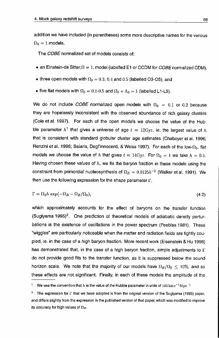
4. Mock galaxy redshift surveys 68
addit ion we have included (in parentheses) some more descriptive names for the various fio = 1 models .
The COBE normal ized set of models consists of:
• an Einstein-de Sit ter ,0 = 1, model (labelled E l or C C D M for COBE normalized CDM),
• three open models with OQ = 0.3, 0.4 and 0.5 ( labelled 0 3 - 0 5 ) , and
• five flat models with QQ = 0.1-0.5 and OQ + Ao = 1 ( labelled L1-L5).
We do not include COBE normal ized open models with = 0.1 or 0.2 because
they are hopelessly inconsistent with the observed abundance of rich galaxy clusters
( C o l e e t a l . 1997). For each of the open models we choose the value of the Hub
ble parameter ii^ that gives a universe of age t w 12Gyr, ie. the largest value of h
that is consistent wi th standard globular cluster age estimates (Chaboyer et al. 1996;
Renzini et al . 1996; Salaris, Degl ' lnnocent i , & Weiss 1997). For each of the IOW-QQ. flat
models we choose the value of h that gives t w 14Gyr. For f2o = 1 we take h = 0.5.
Having chosen these values of h, w e fix the baryon fraction in these models using the
constraint f rom primordial nucleosynthesis of QB - 0.0125/i~^ (Walker e t a l . 1991). We
then use the fol lowing expression for the shape parameter r,
r = noh expi-nB - J ^ B M ) , (4.2)
which approximately accounts for the effect of baryons on the transfer function
(Sugiyama 1995)^. One predict ion of theoretical models of adiabatic density pertur
bat ions is the existence of oscil lations in the power spectrum (Peebles 1981). These
"wiggles" are part icularly noticeable when the matter and radiation fields are tightly cou
p led, ie. in the case of a high baryon fraction. More recent work (Eisenstein & Hu 1998)
has demonstrated that, in the case of a high baryon fraction, simple adjustments to T
do not provide good fits to the transfer function, as it is suppressed below the sound
horizon scale. We note that the majority of our models have f i s / f i o < 10%, and so
these effects are not significant. Finally in each of these models the amplitude of the
1 We use the convention that/i is the value of the Hubble parameter in units of 100 kms"'Mpc"^
^ The expression for r that we have adopted is from the original version of the Sugiyama (1995) paper,
and differs slightly from the expression in the published version of that paper, which was modified to improve
its accuracy for high values of QB-

4. Mock galaxy redshift surveys 69
density perturbat ions Is set so as to be consistent with the COBE measurements of fluctuat ions in the cosmic microwave background (Smoot e t a l . 1992; White & Bunn 1995; Whi te & Bunn 1996). Further details of these models can be found in Cole et al. 1997, which examines the abundance of galaxy clusters in COBE normalized CDM and presents some analysis of clustering of the mass distributions.
For the set of structure normal ized models, we adopt a fixed value of r = 0.25,
as suggested by observat ions of the large-scale structure traced by galaxies (eg.
Maddox, Efstathiou, & Suther land 1996). The ampli tude of the power spectrum Is set ac
cording to the formula as = O . 5 5 0 o w h i c h results In an abundance of rich galaxy clus
ters In reasonably good agreement with observations (White, Efstathiou, & Frenk 1993).
These models include:
• the Einsteln-de Sitter model , E3S. In this chapter we consider two independent re
al izations of this model , E3S A and E3S B. A further eight realizations (C-J) can be
found on our web-si te.
• a ser ies of open models with fio = 0.2-0.5 ( labelled 0 2 S - 0 5 S ) , and
• a series of flat models with QQ = 0.2-0.5 and - F AQ = 1 (labelled L2S-L5S).
Physical ly these models could be produced either by having h = T/Qo or by a change
f rom the standard model of the present energy density in relativistic particles. For exam
ple the ESS model is very similar to the T C D M model of Jenkins et al. (1998), which is
mot ivated by the decaying particle model proposed by Bond & Efstathiou (1991), where
late decay of the r -neutr ino results in the epoch of matter-domination being delayed, and
hence the effective value of r being reduced. The final model listed in table 4 . 1 , E4
( S C D M ) , is the "standard" C D M model , (EInstein-de Sitter with T = h = 0.5), normalized
by the abundance of galaxy clusters.
We consider one further model that falls into both the COBE and structure normalized
categor ies: the ti lted Einstein-de Sitter model , E2 (tilted). For this model, the above
constraints have been appl ied in relating the baryon fraction Q,B, the Hubble parameter
h, and the shape parameter r. In addit ion, the slope, n, of the primordial power spectrum
has been adjusted so that the clustering ampli tude matches COBE observations at large
scales whi le s imultaneously achieving erg = 0.55, as required for consistency with the
observed cluster abundances.

4. Mock galaxy redshift surveys 70
This procedure results in a tilted primordial spectrum with n = 0.803 and a transfer funct ion with r = 0.4506 as given by equation 4.2. In normalizing to the C O S E observat ions, we have included a gravitational wave contribution as predicted by the power-law model of inflation. For this model , gravitational waves contribute approximately 55% of the rms temperature f luctuations on the scales probed by COBE.
4.3 /V-body s imulat ions
We now descr ibe how the initial condit ions of the simulations were set up, how the
simulated mass distribution was propagated to the present day, and how the particles
label led as galaxies were selected.
4.3.1 Initial conditions
Before imposing the desired perturbations, we set up a uniform density field using the
technique descr ibed by White (1996) and Baugh, Gaztanaga, & Efstathiou (1995) to gen
erate a part icle distribution with a "glass" configuration. Particles are placed randomly
throughout the simulat ion box and then evolved with the A/-body code, but with the sign
of the gravitational forces reversed. We used large t imesteps that were approximately
logahthmical ly spaced in expansion factor and evolved the distribution until the gravita
t ional forces on all part icles practically vanished. With this approach, the initial particle
distr ibution is not regular, but the small random fluctuations in the particle density field
do not seed the growth of spurious structures. Simulations with glass and grid initial
condit ions have been found to give very similar statistical results once they are evolved
into the nonl inear regime (White 1996; Baugh, Gaztanaga, & Efstathiou 1995), but the
simulat ions with glass initial condit ions have the advantage that they do not retain an
unseemly grid signature in uncol lapsed regions.
Each of the simulat ions was of a periodic box of side 345.6/i"^ Mpc (192 cells of length
1.8/i~^ Mpc). For each, we created a Gaussian random density field on a 192^ grid, using
the same Fourier phases f rom one model to the next, but varying the mode amplitudes
accord ing to the model power spectrum. We applied the Zel'dovich approximation (Ap
pendix A) to this density field to compute displacements and peculiar velocities at each
grid point. Each particle is displaced from its glass position according to the displace-

4. Mock galaxy redshift surveys 71
merits interpolated from the grid values. Tlie initial expansion factors of the simulations Oj, listed in table 4.1, were determined by setting the amplitude of the initial power spectrum at the Nyquist frequency of the particle grid to be 0.3^ times that for an equivalent Poisson distribution of particles. The Nyquist frequency is the minimum resolvable wavelength of the distribution,
= = 3 l f ^ c (4-3)
where n is the mean particle density. Thus, Pinitiai(%yq) = 0.3^/n. The resid
ual power in the glass configuration is only 0.5% of that in a Poisson distribution at
the Nyquist frequency and drops very rapidly at longer wavelengths (see figure A2 of
Baugh, Gaztanaga, & Efstathiou 1995). This choice is safely in the regime where:
• the initial density fluctuations are large compared to those present in the glass, but
• the Zel'dovich approximation remains accurate.
In particular, no shell-crossing has occurred.
4.3.2 Evolution
We evolved the simulations using a modified version of Hugh Couchman's Adaptive
Particle-Particle-Particle-Mesh (AP^M, Couchman 1991) N-hody code. We set the soft
ening parameter of AP^M's triangular-shaped cloud force law to = 270/i"^ kpc, 15%
of the grid spacing. The softening scale is fixed in comoving co-ordinates. This choice
corresponds approximately to a gravitational softening length e = r)/3 = 90/ i "^kpc for
a Plummer force law, and we adopt e as our nominal force resolution. The size of the
timestep A a was chosen so that the following two constraints were satisfied throughout
the evolution of the particle distribution. First, the rms displacement of particles in one
timestep was less than 77/4. Second, the fastest moving particle moved less than 7? in
one timestep. Initially these two constraints are comparable, but at late times the latter
constraint is more stringent, particularly in low OQ simulations. We monitored energy
conservation using the Layzer-lrvine equation (equation 12b of Efstathiou etal. 1985)
and found that, for this choice of timestep, energy conservation with a fractional accuracy
of better than 0.3% was achieved. We also tested the inaccuracy incurred by these

4. Mock galaxy redshift surveys 72
Table 4.1. Simulation Parameters: the first column gives the label of each of the cosmological models;
alternative, more descriptive names for the flo = 1 models are given in parentheses. The following seven
columns give the corresponding values of the density parameter Qo, cosmological constant Ao, Hubble pa
rameter h, age of the universe t, baryon content fis, power spectrum shape parameter r, and normalization
(78 respectively The final two columns give the initial expansion factors, ai, and number of timesteps, A' steps,
used in the simulation.
Model Ao h t/Gyv r 0-8 • steps 03 0.3 0.0 0.65 12.2 0.030 0.172 0.5 0.15 93
04 0.4 0.0 0.65 11.7 0.030 0.234 0.75 0.1 168
05 0.5 0.0 0.6 12.3 0.035 0.27 0.9 0.08 254
L1 0.1 0.9 0.9 13.9 0.015 0.076 0.7 0.15 150
L2 0.2 0.8 0.75 14.0 0.022 0.131 0.9 0.12 220
L3 0.3 0.7 0.65 14.5 0.030 0.172 1.05 0.101 266
L4 0.4 0.6 0.6 14.5 0.035 0.213 1.1 0.09 275
L5 0.5 0.5 0.6 13.5 0.035 0.27 1.3 0.07 331
02S 0.2 0.0 - - - 0.25 1.44 0.028 447
OSS 0.3 0.0 - - - 0.25 1.13 0.050 313
04S 0.4 0.0 - - - 0.25 0.95 0.073 258
053 0.5 0.0 - - - 0.25 0.83 0.096 212
L2S 0.2 0.8 - - - 0.25 1.44 0.057 405
L3S 0.3 0.7 - - - 0.25 1.13 0.080 287
L4S 0.4 0.6 - - - 0.25 0.95 0.102 224
L5S 0.5 0.5 - - - 0.25 0.83 0.122 184
E1 (CCDM) 1.0 0.0 0.5 13.1 - 0.5 1.35 0.061 327
E2 (tilted) 1.0 0.0 0.5 13.1 0.05 0.45 0.55 0.20 200
E3S (rCDM) 1.0 0.0 - - - 0.25 0.55 0.21 103
E4 (SCDM) 1.0 0.0 0.5 13.1 — 0.5 0.55 0.15 170

4. Mock galaxy redshift surveys 73
choices of starting amplitude and timestep by comparing the final particle positions with two additional versions of the E l , J7o = 1 simulations, which were run starting from a fluctuation amplitude a factor of two lower and using timesteps a factor of two smaller. In each case we found that the final particle positions agreed very accurately, with rms differences of less than e. More importantly, the correlation functions of the particle distributions in all cases were indistinguishable at scales larger than e = 90h~'^ kpc. Thus, the statistical clustering properties of these simulations have a resolution that is limited by the particle mass and force softening and not by the choice of timestep or starting redshift.
4.4 Biasing the galaxy distribution
In this section we describe the methods used to select the particles labelled as galaxies
from the distributions of mass produced in the A/-body simulations. A one-to-one corre
spondence of the galaxy field to the mass field is unlikely. For galaxies to be unbiased
tracers of the underlying mass distribution, the ability to form a galaxy must be indepen
dent of the properties of the surrounding density field, so that each mass particle, no mat
ter where it resided, was equally likely to be associated with a galaxy. Simple, physically
motivated models such as the high peaks model (Davis et al. 1985; Bardeen et al. 1986)
illustrate how a dependence of galaxy formation on the properties of the local density
field can make the galaxy distribution more strongly clustered than the underlying mass
distribution. This effect can be quantified in terms of a bias factor bR = CTI^'/C^H^^ relating
the fractional rms fluctuation in the number of galaxies in spheres of radius Rh''^ Mpc to
the corresponding variation in the mass. For any model in which galaxies form in the
collapse of dark-matter haloes, this relationship must break down on the very smallest
scales simply because a galaxy has much smaller spatial extent than its halo. The
processes of galaxy formation, locally extremely complex, can still result in a large-scale
bias factor of unity.
Observational evidence for bias is presented by Peacock & Dodds (1994). They as
sume a simple, constant linear bias model in which a perturbation in the mass distribution
is accompanied by an amplified perturbation in the galaxy distribution, Jgai = bSmass- They
find that the power spectra of differently selected galaxy samples require a bias relative
to the power spectrum of /flyAS galaxies, V^IRAS. given by:

4. Mock galaxy redshift surveys 74
b/biRAs = 1-3 for optically selected galaxies b/biRAs = 1-9 for radio galaxies b/bmAs = 4.5 for Abell clusters.
Since a relative bias exists between any two of these differently selected samples,
it seems natural to assume that all galaxy samples will be subject to some degree of
bias relative to the underlying mass. We note that bias is also important in interpret
ing the estimates of the mass-to-light ratio of galaxies in clusters. These have been
used in conjunction with estimates of the galaxy luminosity function to infer QQ « 0.2
(Carlberg, Yee, & Ellingson 1997). This inference assumes that galaxies are unbiased
tracers of the mass distribution. If galaxies form preferentially in proto-cluster environ
ments, then this estimate translates to O o / 5 w 0.2, where B is the factor by which the
efficiency of galaxy formation is enhanced in regions destined to become clusters, relative
to the field.
Since the physics of galaxy formation is very complex, we cannot yet determine the
function that relates the probability of forming a galaxy to the properties of the mass
density field, though first steps towards this goal have been taken using cosmological
simulations with gas dynamics (Cen & Ostriker 1992; Katz, Hernquist, & Weinberg 1992;
Summers, Davis, & Evrard 1995; Frenketal. 1996) and with semi-analytic models of
galaxy formation (Benson et al. 1999; Kauffmann, Nusser, & Steinmetz 1997). For this
reason we take the approach of defining the biasing algorithm in terms of a simple
parametric function. Then for each cosmological model we constrain the values of the
function's parameters using estimates of observed small and intermediate scale galaxy
clustering. For a subset of the cosmological models we repeat this procedure for several
different biasing algorithms. Making this repetition, one can quantify the extent to which
the properties of the catalogues depend on the choice of adopted biasing algorithm.
For optically selected galaxies in the ARM survey the clustering amplitude is found to
be af^' - 0.96 (Maddox, Efstathiou, & Sutherland 1996). Many of our simulations have
higher amplitudes than this, and therefore require an anti-bias (6 < 1) on the 8/ i "^ Mpc
scale. Anti-bias seems less physically motivated than bias because it requires negative
feedback processes to suppress galaxy formation in high-density regions. Such an anti-
correlation, however, might be produced even if the production rate of galaxies in proto-

4. Mock galaxy redshift surveys 75
clusters is higher than in low-density regions, so long as galaxy merging in the proto-clusters is sufficiently efficient to suppress the overall number of galaxies in clusters. Alternatively, in an A/-body treatment where haloes are assumed to be spatially exclusive, if each collapses to produce a single galaxy then the galaxies cannot be closer together than the radii of the haloes, so the galaxy distribution cannot match the mass distribution in high density regions. This leads to an anti-bias on scales of order the halo size.
The biasing schemes we consider are, with one exception, local, in the sense that
the probability of a mass particle being selected as a galaxy is a function only of the
neighbouring density field, eg. the density field smoothed on a scale 3h~^ Mpc. Such
models have the property that, on scales (in the linear regime) that are much larger than
that defining the local neighbourhood, they produce a constant, scale independent bias
(Scherrer & Weinberg 1998). A derivation of an expression for this asymptotic bias is
given in section 4.4.2 below. Our algorithms include both Lagrangian models, in which
the selection probability is a function of the initial density field, and Eulerian models, in
which the probability is a function of the final mass density field. For a consideration of
the differences between these approaches see Mann, Peacock, & Heavens 1998.
We use seven different prescriptions for creating the biased galaxy samples. All of them
involve defining a probability field from either the initial or the final density distribution,
and then Poisson sampling the simulation particles using this field to define the selection
probability. The probability is normalized such that a mean of 128^ out of the original 192^
particles are selected. The corresponding galaxy number density is fig « 0.05/i^Mpc~^,
which approximately equals that of galaxies brighter than L* /80 . Although this density is
less than that of the original simulation, occasionally the bias may demand that in certain
regions there is a greater galaxy density than the original particle density. The Poisson
sampling achieves this by allowing some particles to be selected more than once. This
double sampling is generally rare but does occur, especially in the highly biased models.
The functions defining the selection probability have one or two free parameters. In the
case of those with just one free parameter, we fix its value by demanding that ' = 0.96,
in agreement with the value estimated from the APM galaxy survey The models with
two parameters enable us to control both the amplitude of galaxy clustering on large
scales and, to some extent, the slope of the galaxy correlation function on small scales.
We set their parameters by attempting to match simultaneously the observed variance

4. Mock galaxy redshift surveys 76
of the galaxy density field in cubic cells of 5 and 20h~^ Mpc on a side. We assume
c^ceiis = 2.0 and CTceii2o — 0.67, the values from the power spectrum shape estimated
for ARM galaxies by Baugh & Efstathiou (1994), scaling its amplitude for consistency
with the more recent estimate of af^' = 0.96. In some cases, where, for instance, the
small scale mass correlation function is very much steeper than the observed galaxy
correlation, it does not prove possible to simultaneously satisfy these two constraints. For
computational simplicity and to avoid any ambiguity, we choose, in all cases, to fit the
observed values by minimizing the cost function
= ( ( - 5 i 2 _ i m ) ^ + i ^ ^ ^ ^ ^ S + '-'"^ + "^'^ <^-^>
where a and /? are the two model parameters. The third term has ec = 4 x 10"^, and
is included to avoid extremely large values of |Q!| and being selected for very little
improvement in the values of o-ceiie and C7ceii20-
4.4.1 Biasing algoritlims
Here we define the selection probability functions, P(z/), which define each of our biasing
algorithms. The resulting biased galaxy correlation functions, ^(r), and power spectra,
P{k), are shown in Figs. 4.1, 4.2, and 4.3 and discussed below. The biasing algorithm
that we apply to all of the cosmological models is model 1; the other biasing models are
used only to create additional mock catalogues for the 04S, L3S, and E3S simulations.
1. Exponential method: Lagrangian. This model bases the selection probability on the
value of the smoothed initial density. We use a Gaussian smoothing of exp{-r'^/2Rl),
with width Rs = 3 / i~^Mpc to define a smoothed density field, ps ( r ) . at the initial
particle position. We find this field by taking the initial density field, which is defined
on a grid convolving with the smoothing function using an FFT method.
A dimensionless variable, ly, is defined: v{r) = 5s{r)/as, where 5s is the smoothed
overdensity field and a | = (|(5sp). We then adopt
PHcxl ^ - , (4.5) [ exp(ajv) if 1/ < 0
as the selection probability. The model has two free parameters a and j3. This choice
of functional form is essentially selected for its simplicity. Its exponential behaviour

4. Mock galaxy redshift surveys 77
ensures that the probability cannot be negative. The dependence on /3 for > 0 enables the selection probability to be enhanced (/? > 0) or suppressed (/? < 0) in the densest regions. This property gives some control over the slope of the small scale correlation function. The choice of a v'^/'^ dependence is made so that the probability converges when integrated over a Gaussian distribution of v.
2. Exponential method: Eulerian. For this model the same functional form (equa
tion 4.5) is used to define the selection probability, but this time the variable v is defined
in terms of the smoothed final density field around each particle. Again, a Gaussian
smoothing with i?s = 3/i~^ Mpc is adopted.
3. High peaks model. The standard high peaks model of Bardeen et al. (1986) is used
to predict the number of peaks of amplitude u > defined on the scale of a galaxy
as a function of the density smoothed on a larger scale that is resolvable in our
simulation. In this case we choose the larger scale to be defined by applying a sharp
cutoff to the power at a wavelength A 4/ i~^ Mpc, which is quite well resolved in the
initial conditions of the simulation. We define the galaxy mass scale by a Gaussian
smoothing with i?s = 0.54/i~^ Mpc, as adopted by White et al. (1987). Here the model
parameter is v^. An unavoidable property of assuming that galaxies form in peaks of
the density field is that they are more clustered than the mass distribution (6 > 1).
Thus this method cannot be applied in cases where an anti-bias is required.
4. Threshold bias. In this model a sharp cut-off is applied to the final smoothed density
field, so that galaxies are entirely prohibited from forming in very underdense regions,
but have an equal chance of forming wherever the overdensity rises above a certain
threshold, pT- Thus
{ 1 if p{v) > PT P{i^) a I . (4.6)
[ 0 if p(r) < pT
This is the case if a bias greater than unity is required. For an anti-bias, the conditions
are reversed and galaxies are prohibited from forming in the very densest regions.
Note that this prescription for producing anti-bias has unphysical consequences, as it
implies that the highest mass density regions have no galaxies in them at all.

4. Mock galaxy redshift surveys 78
5. Power-law method. As in model 2 the selection probability is defined in terms of the smoothed final density, but this time the functional form adopted is a power law,
P{iy) (X u'^. (4.7)
Here a positive value of the parameter a will induce a bias (6 > 1) and a negative
value an anti-bias (6 < 1). The bias inferred by Cen & Ostriker (1993) from their
hydrodynamic cosmological simulations has roughly this form, with a « 1.5.
6. Exponential bias: adaptive smoothing. This algorithm is a variation of model 2
and again uses the formula (4.5), but with a different definition of the overdensity
parameter v. Instead of smoothing on a fixed scale of S/i"^ Mpc, the distribution was
adaptively smoothed by setting the density at the position of each particle, p oc l/rfg,
where rio is the distance to the tenth nearest neighbour of that particle. It is hoped
that this adaptive definition of the smoothing scale will result in the better definition
of high-density areas, giving more control of the slope of the bias function on small
scales.
7. Non-local bias. All the above models allow the degree of bias only to be affected
by the locally smoothed density fields, on fairly modest scales. As pointed out by
Bower etal. (1993) longer range effects (eg. positive or negative feedback effects
from nearby proto-galaxies) could mean that the neighbouring density field at rather
larger distances could have an effect on galaxy formation, the so-called "co-operative"
model. We implement a simple, two parameter version of this model, where the bias
probability is defined by a power-law,
P{U) OC (l/ + ;9i/s)". (4.8)
Here, v is the usual, locally smoothed density field, and the field smoothed on a
larger scale (lO/j-^ Mpc). We fit the parameters a and (3 so as to match the ARM
clustering amplitudes, as described above.
The parameters used in the first six, local biasing schemes are shown in table 4.2.
The various galaxy correlation functions and power spectra that result from apply
ing bias model 1 to each of the cosmological simulations are shown in figures 4.1
and 4.2 respectively. The solid data points show the estimates of the correlation
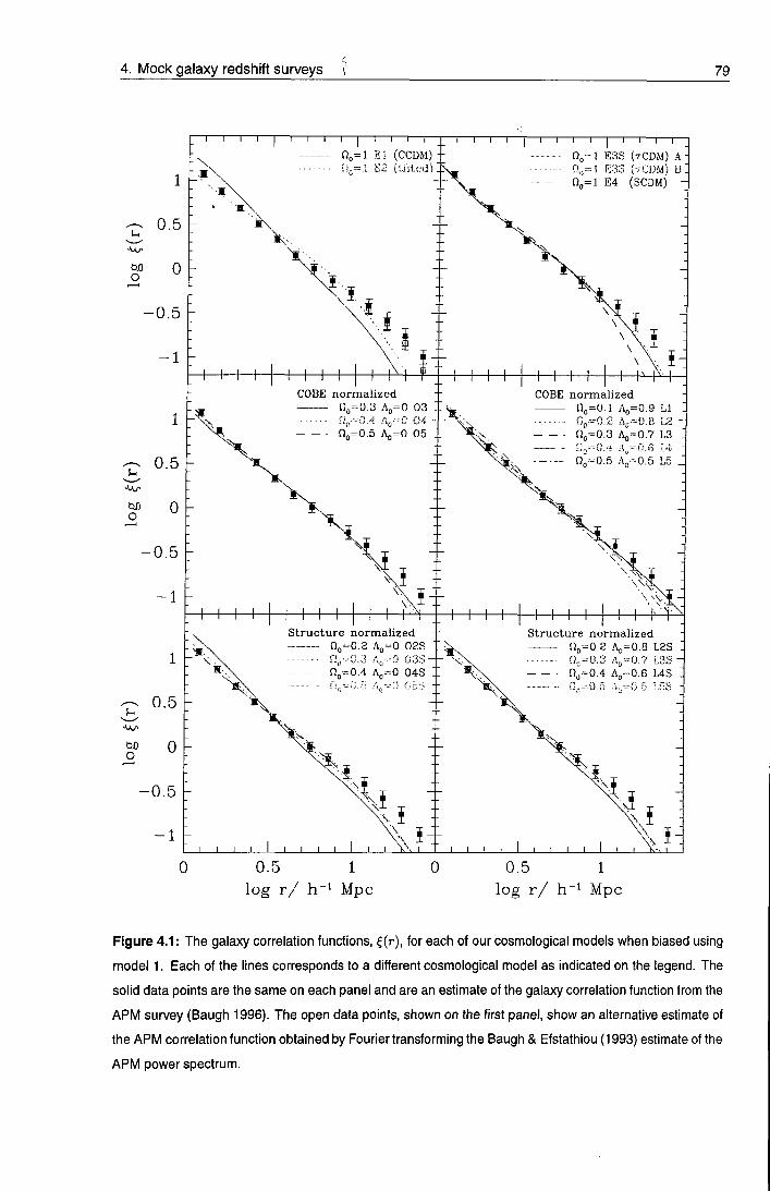
4. Mock galaxy redshift surveys 79
o
Si
o
1
0 ,5
0
- 0 . 5
- 1
1
0 .5
0
-0 .5
- 1
I I I I I I I n „ = l E ! (CCDM)
I i I I I I I I — i
[ l .= l E S S ( T C D M ) A
n . = l E 4 (SCDM)
My
o
C O B E n o r m a l i z e d IJo-O.S A„=0 03 fi„=0.4 A„=0 04
S t r u c t u r e n o r m a l i z e d 0^=0/2 Ao=0 O S S n „ - 0 . 3 A(=0 03S-n „ = 0 . 4 A . = 0 0 4 S
C O B E n o r m a l i z e d n^=0.1 Ao=0.9 L I
n„=0 .5 Ao=0 05 n.=Q.3 A „ = 0 . 7 L3
[L -=0.0 A,= 0.5 Lo
S t r u c t u r e n o r m a l i z e d n„--=0.2 .\o=Q.B L 2 S
Oo=O.S Ao=0.7 L 3 S • n„=o .4 A„=o.6 u s fL ^ 4) 5 A , -o . f t I R S
0.5 1
l o g r / h " ' M p c
0.5 1
l o g r / h " ^ M p c
Figure 4.1: The galaxy correlation functions, | ( r ) , for each of our cosmological models when biased using
model 1. Each of the lines corresponds to a different cosmological model as indicated on the legend. The
solid data points are the same on each panel and are an estimate of the galaxy correlation function from the
APM survey (Baugh 1996). The open data points, shown on the first panel, show an alternative estimate of
the APM correlation function obtained by Fourier transforming the Baugh & Efstathiou (1993) estimate of the
APM power spectrum.
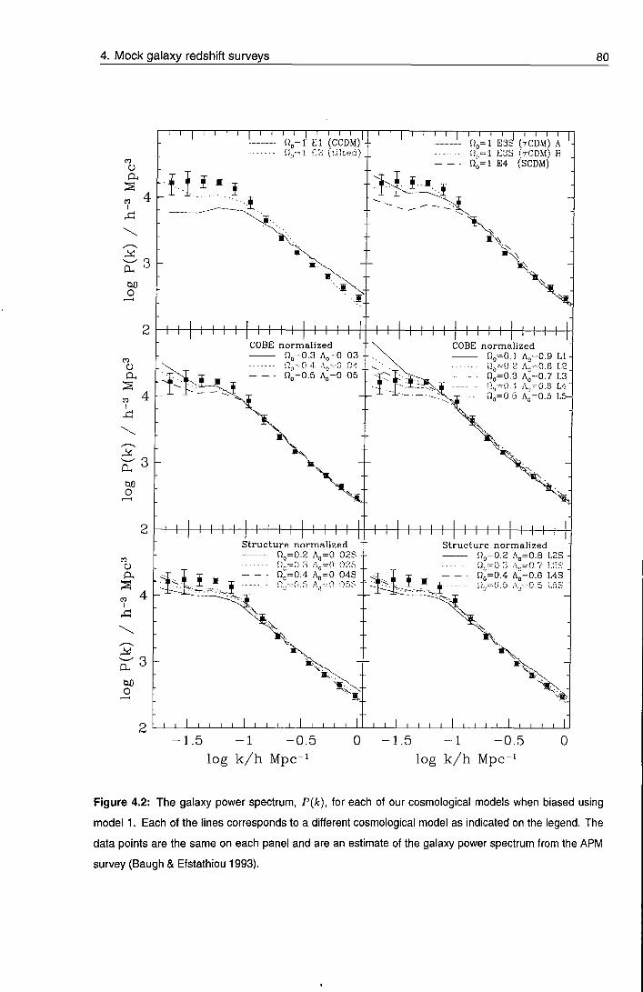
4. Mock galaxy redshift surveys 80
" T — I — I — I — I — I — i — I — I — I — i — i — I — I — I — I — i — I - n „ = l E l ( C C D M )
fi,,= l m fu l l ed )
T—r
o
I I I I I I I I I I
1—I—I—I—i—I—i—I—I—i—i—i—n n„= 1 E 3 ^ ( T C D M ) A
= 1 E3S (rCDM) E Qo=l E4 (SCDM)
I I I M I I I I
n„=0 .3 A.=0.7 L3 0 . 6 lA
n„=0.5 A =0.5 L 5 -I
o
C O B E n o r m a l i z e d no=0.3 A„=0 03
A^-o 0 4 n~=0.5 A„=0 05
COBE n o r m a l i z e d n„=0.1 A,=0.9 L1-]
I M I I I I I I I I I I I I I I I I I I I I I I I I I I
CO O
s t r u c t u r e n o r m a l i z e d %=0.Z A„=0 02S n „ = 0 , 3 A , = 0 OSS
X , n;=0.4 A„=0 04S 1 • I n . -G.5 A , - 0 OSS
s t r u c t u r e n o r m a l i z e d n„=0 .2 A„=0.8 L2S 0 „ = 0 . 3 A " = 0 . 7 U3S no=0.4 A5=0.6 L4S
. . = 0 . 5 LflS
ao o
3 h
- 1 . 5 - 1 - 0 . 5
l o g k / h M p c " ^
0 - 1 . 5 - 1 - 0 . 5
l o g k / h M p c " ' 0
Figure 4.2: The galaxy power spectrum, P{k), for each of our cosmological models when biased using
model 1. Each of the lines corresponds to a different cosmological model as indicated on the legend. The
data points are the same on each panel and are an estimate of the galaxy power spectrum from the APM
survey (Baugh & Efstathiou 1993).

4. Mock galaxy redshift surveys 81
I I i [ I I i i I
M o d e l 1
M o d e l 2
M o d e l 4
;v!od.€
— M o d e l 6
M o d e
M o d e l 1
M o d e l 2
M o d e l 4
M o d e l 5
M o d e l 6
M o d e l 7
^0=0.4 A =0
M o d e l 1
M o d e l 2
M o d e l 4
Mot M o d e l 6
Model 7
Qo=0.3 Ao=0.7
0 0.5 1 log r/h~^Mpc
Figure 4.3: For three selected, structure normalized cosmological models (E3S,04S and L3S), we show the
galaxy correlation functions that result from each of the bias models. Note that both of the Qo < 1 models
require anti-bias and therefore cannot be biased using peaks bias, model 3. The line types corresponding to
each of the bias models are indicated on the legend. The data points again show the estimate of the galaxy
correlation function from the APM survey

4. Mock galaxy redshift surveys 82
Table 4.2. Bias model parameters. For the three selected cosmological models we list the parameter values
required in each of the six local bias models. The resulting galaxy correlation functions are compared in
figure 4.3.
Identifier Model 1 Model 2 Model 3 Model 4 Model 5 Model 6
Q!f /?f PT a af
04S 3.60 -9.05 2.17 -1.31 - <19.7 -0.02 3.96 -2.69
L3S 2.55 -17.75 0.15 -0.06 - <15.5 -0.13 7.11 -7.15
E3S 1.10 -0.56 1.26 -0.51 1.005 >0.98 0.56 2.98 -1.25
function (Baugh 1996) and power spectrum (Baugh & Efstathiou 1993) of APM galax
ies, scaled in amplitude to match the estimate of crf^' = 0.96 for the ARM survey
(Maddox, Efstathiou, & Sutherland 1996). The data points plotted as open symbols on
the top left panel of figure 4.1 show the ARM correlation function as estimated from the
Fourier transform of the estimated ARM power spectrum. There is a slight difference
between this and the direct estimate at large separations, which arises because both ^ ( r )
and P(A;) are estimated using non-linear inversions of the measured angular correlation
function. The difference is an indication of one of the systematic errors involved in
estimating ,^(r) on large scales.
In general, the two-parameter biasing model is successful in matching both the ampli
tude and the shape of the galaxy correlation function on scales of l-10/i~^ Mpc, as can
clearly be seen in figure 4.1. For a few cases, such as E l , 02S, and L2S, which have high
values of a^^^ and consequently steep non-linear mass correlation functions, the bias
model cannot reduce the slope of the correlation function enough to accurately match the
observed value. The behaviour of the correlation functions on large scales reflects each
model's value of the power spectrum shape parameter r. The ARM data, if fitted with a
r-model with no bias, prefer r = 0.15-0.2 (eg. Efstathiou, Sutherland, & Maddox 1990),
so even our structure normalized, V = 0.25 models fall short of the amount of large-
scale power evident in the ARM correlation function. This short-fall is also exaggerated
by a statistical fluctuation in our simulation initial conditions. As can be seen in the top-
right-hand panel of figure 4.2, the first realization (A) of model E3S has less power on
scales 0.03 ^ A; ^ 0.06/iMpc~^ than the second realization (B) of the same model. This
downward fluctuation in the power is present in all the other cosmological models, since

4. Mock galaxy redshift surveys 83
all the initial density fields were generated from the same basic Gaussian random field but with expected mean amplitudes rescaled according to the model power spectrum. We also note that the longest wavelength modes, with k = 2-K/LBOX, are noisy because of the small number of such modes contained in the simulation box. The comparison of model and APM galaxy power spectra on small scales (high k) is in accord with the small scale behaviour of the correlation functions.
The manner in which the galaxy clustering statistics vary with the form of the biasing is
illustrated in figure 4.3. The one-parameter bias models (models 3, 4 and 5) do not have
the flexibility to control both the amplitude and slope of the galaxy correlation function.
Thus, in general, these models do not match the APM galaxy correlation function over a
wide range of scales. In particular, the galaxy correlation functions of the three models
selected for figure 4.3 are steeper than the correlation function of APM galaxies, reflecting
the steepness of the underlying mass correlation functions. The 3/i~^ Mpc filter used
in bias model 2 smooths over the structure of groups and clusters in the final density
field. As a result, the small-scale slope of the galaxy correlation function ends up being
insensitive to the bias model parameters in this case. In model 6, on the other hand,
the use of an adaptive smoothing results in better resolution on the scale of groups and
clusters. In some cases this is enough to enable the required adjustments to the slope of
the correlation function on small scales. Model 7 is substantially better at obtaining the
correct large-scale slope, especially in the IOW-OQ cases. This is unsurprising since this
method depends on the large-scale density field, giving it more "leverage" than the other
models.
4.4.2 The asymptotic bias
In general all the biasing algorithms discussed above give rise to a bias that is scale
dependent. However, since the biasing algorithms used in models 1-6 only depend on
local properties of the density field, the bias should tend to a constant on large scales
(Mann, Peacock, & Heavens 1998). Where the selection probability is a function of the
initial density field, the value of this asymptotic bias can be computed analytically The
probability that a mass particle is selected as a galaxy is taken to be P{u), where i/ is the

4. Mock galaxy redshift surveys 84
amplitude of the initial density fluctuation in units of the rms, o-g. The normalization of P{u) is determined by the integral over the Gaussian distribution of initial density fluctuations,
I P{u)e-^'lUu = l. (4.9)
The density of galaxies selected in a region in which a large scale perturbation A is added
will be given by
Pgal = Pgal / P(^' ) e-^'l' du, (4.10)
where u' = u + A/o-g. In the regime where A/o-g < u, we can accurately approximate
P{u) with its first order series expansion, yielding
P M = P M ( I + ^ ^ ) . (4 .11)
Hence
Pgal ^ 3 ^ ' \ dv o j ^ '
which simplifies to
Pgal
Pgal
We can thus define an asymptotic bias factor, ie. the ratio of the galaxy to the mass
perturbations on large scales, as
fcasymp = ^ ^ ^ ^ / A = 1 + - = U / ^ e - V 2 (4.14)
This result is compared to the bias estimated from the simulations in figure 4.4. The figure
clearly shows that the bias does indeed tend towards its asymptotic value, as calculated
above, on large scales.
4.5 The mock catalogues
The previous section described the procedure by which we create a galaxy distribution
within each simulation cube. We now outline how these are manipulated and sampled
to create the mock galaxy catalogues. It should be noted that we do not attempt to

4. Mock galaxy redshift surveys 85
E 1.5
1
0.5
~ i — I — I — I — I — I — I — I — I — I — I — I — I — I — I — I — I — 1 n„=l' E l (CCDM)'
a , ^ l EZ ( t i l l ed)
E 1.5
0.5
E 1.5
0.5
I I I I I I I I I I I I I
COBE n o r m a l i z e d n„=0.3 Ao=0 03 Qt,^OA h^=Q 04
• n„=0.5 A„=0 05
I I I I I I I I s t r u c t u r e n o r m a l i z e d
00=0-2 Ao = 0 02S O, = 0.3 As,-0 03S
• n.=0.4 A„=0 04S
" T — 1 — I — i — I — i — 1 — I — 1 — i — I — i — 1 — I — 1 — I — r -
0„=1 E3S (rCDM) A 0 = 1 i;3S ( t C D M J B n„=l E4 (SCDM)
I I I I I I I J I I I I I I I I I • COBE n o r m a l i z e d
n „ = 0 . t Ao=0.9 L I
nl=0.3 A„=0.7 L3
fJ(,=^0.5 Aj,=0.5 L6
I I I I I I I I I I I I I I I I I S t r u c t u r e normal i zed
fi„=0.2 /\,=0.8 l.,2S n ,=0 .3 Ap=0,'7 L3S
• 0^=0.4 A„=0.6 L4S 0„='D,5 A , = 0 . 5 L5S
J --1 .5 - 1 -0 .5
log k / h Mpc-' •1.5 - 1 -0 .5
log k / h Mpc"'
Figure 4.4: The scale-dependent bias, b{k) = [Pgii{k)/Pm&ss{k)Y^'', for each of our cosmological models
when biased using bias model 1. Each of the lines corresponds to a different cosmological model as
indicated on the figure. To the right of each panel we show the value of the expected asymptotic bias
on large scales, as explained in section 4.4.2.
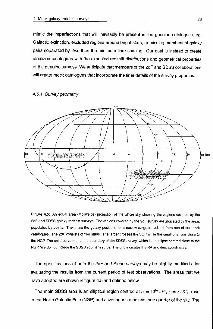
4. Mock galaxy redshift surveys 86
mimic the imperfections that will inevitably be present in the genuine catalogues, eg.
Galactic extinction, excluded regions around bright stars, or missing members of galaxy
pairs separated by less than the minimum fibre spacing. Our goal is instead to create
idealized catalogues with the expected redshift distributions and geometrical properties
of the genuine surveys. We anticipate that members of the 2dF and SDSS collaborations
will create mock catalogues that incorporate the finer details of the survey properties.
4.5.1 Survey geometry
18 hrs
Figure 4.5: An equal area (Mollweide) projection of the whole sky showing the regions covered by the
2dF and SDSS galaxy redshift surveys. The regions covered by the 2dF survey are indicated by the areas
populated by points. These are the galaxy positions for a narrow range in redshift from one of our mock
catalogues. The 2dF consists of two strips. The larger crosses the SGP while the small one runs close to
the NGP. The solid curve marks the boundary of the SDSS survey, which is an ellipse centred close to the
NGP. We do not include the SDSS southern strips. The grid indicates the RA and dec. coordinates.
The specifications of both the 2dF and Sloan surveys may be slightly modified after
evaluating the results from the current period of test observations. The areas that we
have adopted are shown in figure 4.5 and defined below.
The main SDSS area is an elliptical region centred at a = 12^''20'", S = 32.8°, close
to the North Galactic Role (NGR) and covering n steradians, one quarter of the sky. The

4. Mock ga laxy redshif t surveys 87
minor axis of the ellipse spans 110° and runs along a line of constant RA. The major axis spans 130°. Our mock catalogues do not include the strips in the Southern Galactic Cap that will also be part of the SDSS redshift survey; larger simulation volumes are needed to model simultaneously the Northern and Southern SDSS.
The main 2dF survey consists of two broad declination strips. The larger is approxi
mately centred on the SGP and covers the declination range -22.5° > 6 > -37.5°. This
declination range breaks into three contiguous, 5° wide strips, each with slightly different
ranges in RA, which, from north to south are:
1. 2l' '"48™ < a < 3^^24'",
2. 21^'"39.5'" < a < S^'AS.b"" and
3. 21*^^49'" < a < 3'^'"29".
The smaller strip in the northern galactic hemisphere covers -7.5° < S < 2.5° with right
ascension
4. 9'^'"50" < a < 14^'"50'".
Together, the strips cover a solid angle of 0.51 steradians. There is considerable overlap
between the northern slice and the area covered by the SDSS.
4.5.2 The radial selection function
The galaxies of the 2dF survey are selected from the ARM galaxy survey and will be
complete to an extinction corrected apparent magnitude of bj < 19.45. The SDSS will
have galaxies selected from its own multi-band digital photometry. The primary selection
will be made in the r'-band, and it will include a surface brightness threshold to ensure that
an adequate fraction of the galaxy light goes down a 3" fibre (see Gunn & Weinberg 1995
for details). For simplicity, and because our goal is merely to match the geometry and
depth of the two surveys, we make our selection for both catalogues in the 6j-band. For
the SDSS we adopt a magnitude limit of &j < 18.9 so as to approximately reproduce
the SDSS target of 900,000 galaxies in the survey area. A mock catalogue from a
(600/i~^ Mpc)^ A/-body simulation that mimics the SDSS selection function in greater
detail is also undenway (Gott et al. in preparation; see also Gunn & Weinberg 1995). In

4. Mock ga laxy redshif t surveys 88
addition to its primary galaxy sample, the SDSS will target a set of ~ 100,000 luminous red elliptical galaxies, to create a deep, sparse sample that is approximately volume-limited to 2 ~ 0.4. Similarly, the 2dF programme includes a deep extension to i? ~ 21 that will contain ~ 10000 galaxies. We do not attempt to model these samples because their median depths are larger than the simulation cubes.
In order to compute the radial selection functions of the surveys, we adopt a Schechter
(1976) function description of the 6j-band luminosity function,
dL = 4>^ {L/L^r* expi-L/L^) dL/L^, (4.15)
with absolute magnitude M(,j = Mg-2.51ogio(i^/i:'0). We relate the apparent magnitude
6j of a galaxy at redshift z to the corresponding absolute magnitude M(,j at redshift z = 0
using
6j - e + k + 5log^oidL/h-^ Mpc) + 25 + (M^^ - 51ogio h). (4.16)
Here di is the luminosity distance to redshift z in the appropriate cosmological model.
The term "k" denotes the so called k-correction, which arises from the Doppler shift to
the wavelength of the galaxy's spectral energy distribution when viewed in the observer's
frame. The term "e" describes the effect of luminosity evolution in the galaxy as a result
of a combination of passive evolution of the stellar populations and star formation. This
model therefore allows for luminosity evolution, but not for any change in the shape of the
galaxy luminosity function, which might occur as a result of galaxy merging or luminosity
dependent evolution.
Even over the relatively limited range of apparent magnitudes covered by the APM sur
vey, the galaxy number counts are a significantly steeper function of apparent magnitude
than is predicted by non-evolving models (Maddox et al. 1990). In contrast, the K-band
galaxy counts have shown no evidence for such a steep slope (Gardner et al. 1997), but
recently Philips & Turner (1998) have used a compilation of survey data to argue that at
the brightest magnitudes the K-band slope is as steep as that seen in the B-band. Unless
we live in a very large underdense region or there exists some as yet unidentified sys
tematic error in the bright galaxy counts (Bertin & Dennefeld 1997; Metcalfe et al. 1991),
some form of rapid galaxy evolution is necessary. The counts can be reproduced by a
model with strong luminosity evolution such as can be accommodated in equation 4.16,
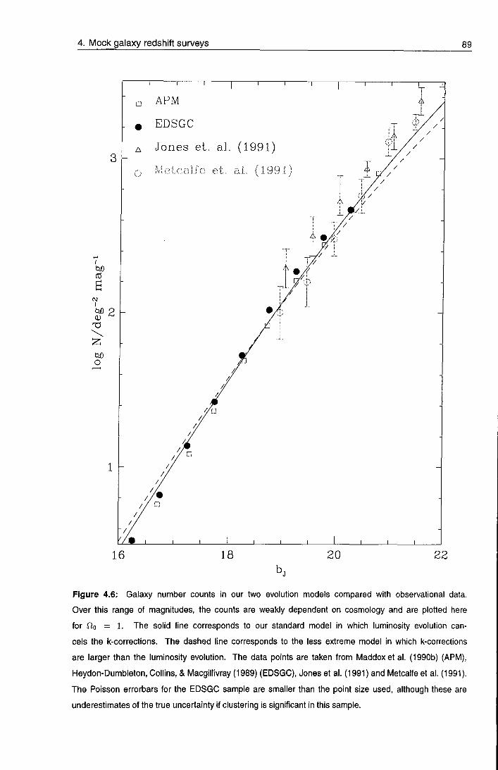
4. Mock ga laxy redshif t surveys 89
T i r 1 1 r
cd
CD
O
• APM
« EDSGC
A Jones et. al. (1991)
O :M:etcal.ie et, ai, (1991)
J I L J I L
16 18 20 22
Figure 4.6: Galaxy number counts in our two evolution models compared with observational data.
Over this range of magnitudes, the counts are weakly dependent on cosmology and are plotted here
for fio = 1. The solid line corresponds to our standard model in which luminosity evolution can
cels the k-corrections. The dashed line corresponds to the less extreme model in which k-corrections
are larger than the luminosity evolution. The data points are taken from Maddoxet al. (1990b) (APM),
Heydon-Dumbleton, Collins, & Macgillivray (1989) (EDSGC), Jones et al. (1991) and Metcalfe et al. (1991).
The Poisson errorbars for the EDSGC sample are smaller than the point size used, although these are
underestimates of the true uncertainty if clustering is significant in this sample.

4. Mock ga laxy redshif t surveys 90
8
isi
n < > \ , , r -f 1 1 r
SDSS
0.4
Figure 4.7: The model galaxy redshift distributions. These distributions are weakly dependent on cosmology
and are plotted here for Qo = 1- The heavy curves, peaking at the higher redshifts, correspond to the
magnitude limit of 6j < 19.45 of the 2dF survey and light lines to the 6j < 18.9 of the SDSS. As in figure 4.6,
the solid curves are for our standard selection function and the dashed curves for the alternative model
with weaker luminosity evolution. The median redshifts are «m = 0.13 and 0.12 for the 2dF catalogues and
z = 0.11 and 0.10 for the SDSS catalogues.
but, at fainter magnitudes than those covered by the SDSS and 2dF surveys, such a
model predicts a tail of high redshift galaxies that is not seen in deep spectroscopic galaxy
samples (eg. Colless et al. 1990). Thus, a more complicated form of evolution is required,
either one in which different galaxies evolve at different rates or one in which galaxies
merge so that their number is not conserved. The new redshift surveys themselves will
give important information on evolution of the galaxy luminosity function. However, for the
purposes of quantifying large structure this is not a problem provided that the selection
function can be accurately determined. We have therefore adopted a simple model that
produces a selection function with similar depth to that which we expect the surveys to
have.
In our standard model we adopt the parameters found by Loveday et al. (1992) for the
APM-Stromlo bright galaxy survey:

4. Mock ga laxy redshif t surveys 91
M * -51ogio/j = -19.5 ,
= -0.97 ,
<i)^ = 1.4 X 10⁻²/i3Mpc-3 .
We also set k + e = 0, ie. we assume that strong luminosity evolution occurs, cancelling
the k-correction. While this cancellation seems coincidental, figure 4.6 shows that this
simple choice gives reasonable agreement with the observed galaxy number counts at
Bj ^ 19.5 and so will produce mock galaxy catalogues with approximately the number of
galaxies expected in the 2dF survey.
As a variation, we have also produced a selection of mock catalogues in which the
artificial assumption that k -f e = 0 has been dropped. For these we use the evolution
law k + e = 2.5 logio(l + z), which corresponds to weaker luminosity evolution than in our
standard model. To compensate for this we increase the value of by 24% to keep the
total number of galaxies in the survey approximately the same as in our standard model.
This model's galaxy counts and redshift distributions (for the case of OQ = 1) are shown
by the dashed lines in figures 4.6 and 4.7.
More recent observational data now exists concerning the faint end of the luminos
ity function. The ESQ slice project, a redshift survey of three thousand galaxies with
magnitude limit bj = 19.4, find a steeper function, parameterized by a* = -1.22
(Zuccaetal . 1997). This would result in more objects at lower redshift, and a lower
median redshift for the surveys.
4.5.3 Survey construction
The task of generating a mock galaxy catalogue now consists of two steps: choosing the
location of the observer, and selecting galaxies subject to the geometrical constraints and
radial selection function specified above.
To aid in the comparison between the different cosmological models, we choose to
place the observer at the same position in each of the galaxy catalogues. The observer's
position was essentially chosen at random, although we did apply the weak constraint that
the velocity dispersion of particles within 5/i"^ Mpc of the observer should be less than
350km in the 1] = 1 model, in order to avoid observers placed in rich galaxy clusters.

4. Mock galaxy redshift surveys 92
This constraint was only directly applied in model ESS, but by virtue of the fact that all the simulations have the same phases it is effectively satisfied in all the structure normalized models. However, for the COSE normalized simulations that have greater than that required to match the observed abundance of rich clusters, the galaxy velocity dispersion is typically higher, and the constraint may be violated. For most analyses of the 2dF and Sloan surveys the choice of the observer should not be important, as the volumes of the surveys are large compared to the local region whose properties are constrained by the choice of observer.
Having chosen the observer's location, we replicate the periodic cube of the /V-body
simulation around the observer to reach a depth oi z = 0.5. We choose the same
position for the observer in both the 2dF and SDSS surveys, but the relative orientations
were not chosen to be consistent with the true angular positions of the two surveys. We
then loop over all the galaxies within the geometrical boundaries of the survey From
the model luminosity function and cosmology we compute the expected mean number
density ns(r) of galaxies brighter than the survey magnitude limit at the distance r of
each of these galaxies. We then select the galaxy zero, one or more times according to a
Poisson distribution with mean ns(r)/ng, where fig is the mean galaxy number density in
the biased galaxy distribution described in section 4.4. In this process, approximately
1% of the galaxies are selected more than once and appear with identical positions
and velocities in the mock catalogue. This double sampling essentially never occurs
at z > 0.02, where the selection function drops to a space density less than ng. For
each selected galaxy we generate an apparent bj magnitude consistent with the selection
function, and also a value of ^max. defined as the redshift corresponding to the maximum
distance at which the younger counterpart of the galaxy would still be brighter than the
survey apparent magnitude limit. In computing this redshift we include the effect of both
the k-correction and evolution on the galaxy's luminosity. As our idealized models assume
that galaxy mergers do not take place, this definition of Zmax makes it easy to construct
volume limited catalogues in which the mean galaxy density is independent of redshift.
For the genuine surveys, removing the effect of evolution from the radial dependence of
the galaxy density field will be more problematic; evolutionary corrections for each galaxy
will be uncertain, and, even over the limited redshift range probed by these surveys,
galaxy merging may also play a small role. In our catalogues we record the galaxy
redshift, its angular coordinates, the redshift it would have if it had no peculiar velocity, its

4. Mock galaxy redshift surveys 93
apparent bj magnitude, and Zmax- We also record an index that can be used to identify the particle to which it corresponded in the original A/-body simulation. These records are explained in detail in section 4.8.
4.5.4 Adding long wavelength power
For a subset of simulations we have applied a technique that allows the spectrum of
density fluctuations present in the final galaxy catalogues to be extended to wavelengths
longer than those included in the original N-hody simulation. This method, dubbed the
Mode Adding Procedure (MAP), was proposed by Tormen & Bertschinger (1996) and
discussed further by Cole (1997). Essentially, one uses the Zel'dovich approximation with
a change of sign to remove from the initial A/-body particle distribution the displacements
caused by the longest wavelength modes in the original simulation. This procedure is
accurate if the modes in question are still in the linear regime. One then generates a new
large scale density field in a much larger box, which samples this same region of ib-space
more finely Displacements are computed by the Zel'dovich approximation from this new
field and used to perturb both the original simulation cube and the adjacent replicas. The
displacements applied to each of the replicas differ, as the new large scale density field is
not periodic on the scale of the original simulation cube. We choose to remove the inner
5 modes from the original simulations and generate the large scale density field in a box
with edge seven times that of the original simulation (A^s = 2 and L/S = 7\n the notation
of Cole 1997).
As pointed out by Cole (1997), the biasing algorithm must take account of the effect
of the added long wavelength power. This is most easily done for algorithms such as
model 1, which are a function of the initial linear density field. One simply replaces
the original linear density field by a new one constructed by removing the original long
wavelength power and adding the new large scale density field. It is more complicated to
correctly apply a biasing algorithm that is a function of the final density field, because the
final density field is non-linear, and its short wavelength modes are coupled to the linear
long wavelength modes. With this in mind, we applied the MAP only in combination with
bias model 1. In order to keep computer storage requirements within reasonable bounds,
it is necessary to combine into a single program the application of the MAP, the biasing
prescription, and the survey selection criteria.

4. Mock ga laxy redshif t surveys 94
4.5.5 Inventory
For each of the cosmological simulations listed in table 4.1 (21, including the second
realization of model E3S), we have created mock SDSS and 2dF surveys using bias
model 1 and the standard selection function, in which the evolution and k-corrections
cancel. The MAP was not used to add long wavelength power to these catalogues. For
four structure-normalized cosmological simulations (the open OQ = 0.4 model (04S), the
flat Cto = 0.3 (L3S), and the A and B realizations of the Einstein-de Sitter model (E3S)) we
constructed a number of variants: changing the bias model to models 2, 3, 4, 5, 6, and 7;
without bias; using the variation of the selection function described in section 4.5.2, in
which luminosity evolution is weaker than the k-corrections; and using bias model 1 with
long wavelength power added using the MAP.
4.6 Illustrations
We now compare and contrast the visual properties of the galaxy distributions in each of
the mock catalogues using a series of redshift space wedge diagrams.
Figures 4.8 and 4.9 show the galaxy distribution in redshift space slices extracted from
the mock 2dF and S D S S catalogues constructed from the cluster-normalized A/-body
simulations. Each of the catalogues was biased using model 1 of section 4.4. The 2dF
slices (figure 4.8) are 90° wide in RA, 3° thick in declination and plotted out to a redshift of
z = 0.3. By contrast, the S D S S slices (figure 4.9), which are 130° wide (corresponding to
the full length of the long axis of the S D S S ellipse) are 6° thick but plotted only to 2 = 0.2.
A visual inspection reveals that the structure in all six models looks remarkably similar.
This is essentially a reflection of the facts that all the simulations were started with the
same phases and that the observer is alway located at the same position. Also, because
these models are designed to produce similar abundances of rich galaxy clusters, the
strength of the "fingers-of-god" effect is also similar. The 1 -dimensional galaxy velocity
dispersions in all the cluster-normalized models is in the range 440-465kms~^ The visible
effects on the galaxy distribution that result from varying Qq, AQ, and the amount of large
scale power ( T ) are quite subtle. Of the two fio = 1 models, E3S ( T C D M ) has more large
scale power than E4 ( S C D M ) . A manifestation of this is that structure in E3S (rCDM)
appears more connected and less choppy than that of E4 ( S C D M ) . The changes that

4. Mock ga laxy redshif t surveys 95
E4 (SCDM)
a.=.0.55 17,=0.55
Galaxies Mass Galaxies
n.=o.5
cr.=0.B3
Mass
^^^^ f"#f
n.=o.5
,=0.B3
Galaxies
n.=o.2
Si,
Figure 4.8: Redshift space slices showing galaxy positions from a variety of the mock 2dF galaxy catalogues.
Each wedge shows a strip 90° wide in R.A. and 3° thick in declination, extending to ^ = 0.3. Each of the six
models shown is normalized by the present abundance of galaxy clusters and biased using model 1 (see
section 4.4). The inset square panels illustrate the effect of bias by showing the real space particle and
galaxy distributions in a 100 x 100 x 20h~^ Mpc slab. The top panels show fio = 1 models: E3S (rCDM)
on the left and E4 (SCDM) on the right. Below these are the open and flat flo = 0.5 models, 0 5 5 and L5S,
and, at the bottom, the open and flat Qo = 0.2 models, 02S and L2S.

4. Mock galaxy redshift surveys 96
E4 ( S C D M )
E S S (TCDM) A.=0
(7,=0.55
n.=o.5 A,=0 1I.=0.83
n,=o.5 A.=0.5
0.63
= 1.44
"0=0.2 A„=0.8
Figure 4.9: Redshift space slices from the cluster normalized mock SDSS catalogues. The correspondence
between model and panel is the same as for figure 4.8. The slices are 130° wide by 6° thick and extend to
z = 0.2. The qualitative differences between the structure visible in these slices and in the corresponding
2dF slices of figure 4.8 are due to the choice of slice thickness and depth rather than any intrinsic difference
in the 2dF and SDSS selection functions.

4. Mock galaxy redshift surveys 97
EZ (tilled)
n.-o.5 A.=0 ",=0.9
Galaxies Galaxies
n.=o.4 n.=o.3 A.=0 (r,=0.75
Galaxies 111
Figure 4.10: Redshift space slices from the mock 2dF catalogues for the tilted CDM model E2 (top left) and
the open COSE normalized models, 05 , 0 4 , and 03 . The corresponding value of Qo and the normalization
£78 are indicated on each panel. The geometry of the slices and inset plots of the real space mass and galaxy
distributions is the same as in figure 4.8.
occur when f2o is varied are related to the strength of galaxy biasing. For models that are
normalized to produce the observed abundance of rich clusters, the amplitude of mass
fluctuations, as, increases as fio is decreased. Thus, the OQ = 1 models require a strong
bias, the OQ = 0.5 models a weak bias, and the QQ = 0.2 models an anti-bias. The
effect of this can be seen most clearly in the inset square panels of figure 4.8. These
show, in real space, a 100 x 100 x 20h~^ Mpc slab of the mass and corresponding galaxy
distribution, both sampled to the same density of fig « O.Obh^Mpc'^. In the OQ > 0.5
models, the biasing algorithm clearly has the effect of mapping underdense regions in the
mass distribution to completely empty voids in the galaxy distribution. In the anti-biased,
Qo = 0.2 models, galaxies continue to trace the mass in the underdense regions. Finally,
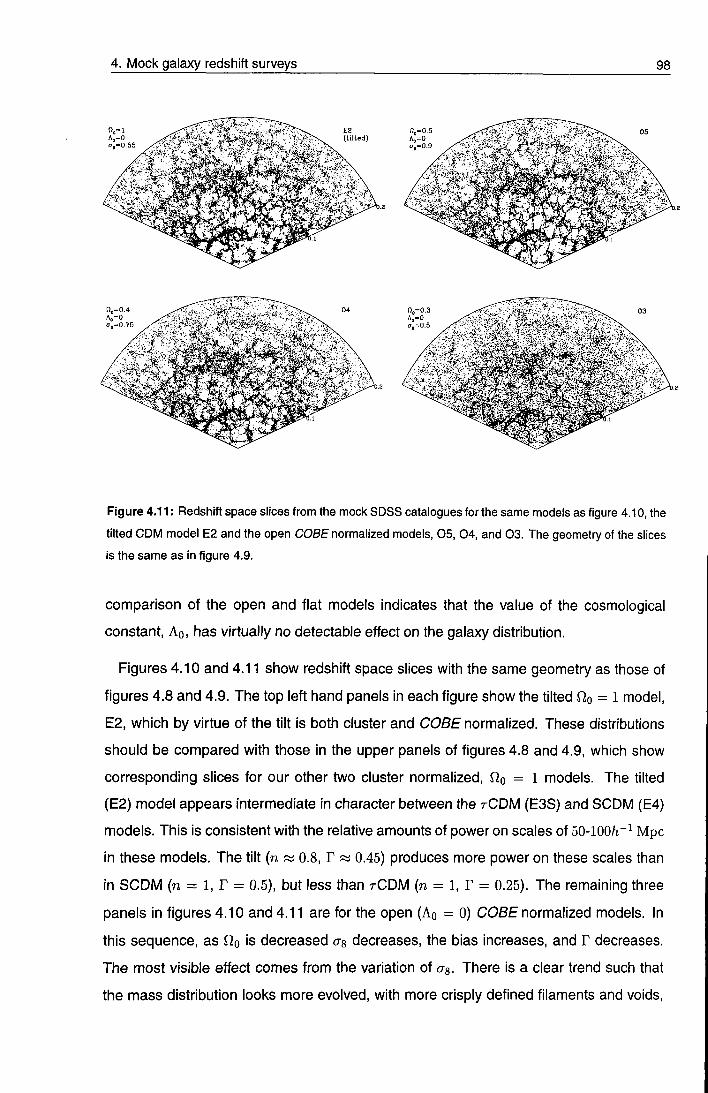
4. Mock galaxy redshift surveys 98
A,=0 o,=0.55
E2 (tilted)
" 0 = 0 . 5 A . = 0
" 0 = 0 . 4 A,=0 <7,=0.75
" 0 = 0 . 3 A.=0 <T,=0.5
Figure 4.11: Redshift space slices from the mock SDSS catalogues for the same models as figure 4.10, the
tilted CDM model E2 and the open COBE normalized models, 05 , 0 4 , and 03 . The geometry of the slices
is the same as in figure 4.9.
comparison of the open and flat models indicates that the value of the cosmological
constant, AQ, has virtually no detectable effect on the galaxy distribution.
Figures 4.10 and 4.11 show redshift space slices with the same geometry as those of
figures 4.8 and 4.9. The top left hand panels in each figure show the tilted = 1 model,
E2, which by virtue of the tilt is both cluster and COBE normalized. These distributions
should be compared with those in the upper panels of figures 4.8 and 4.9, which show
corresponding slices for our other two cluster normalized, Jo = 1 models. The tilted
(E2) model appears intermediate in character between the rCDM (E3S) and SCDM (E4)
models. This is consistent with the relative amounts of power on scales of 50-100/i~^ Mpc
in these models. The tilt (n w 0.8, r w 0.45) produces more power on these scales than
in SCDM (n = 1, r = 0.5), but less than rCDM (n = 1, r = 0.25). The remaining three
panels in figures 4.10 and 4.11 are for the open (Ao = 0) COBE normalized models. In
this sequence, as CIQ is decreased as decreases, the bias increases, and r decreases.
The most visible effect comes from the variation of ag. There is a clear trend such that
the mass distribution looks more evolved, with more crisply defined filaments and voids.

4. Mock ga laxy redshif t surveys 99
E l (CCDM) n,=o.5
o.= 1.3
Mass Galaxies Ga axles
1 > v t ' T
o.= 1.05
Galaxies
n.=o,2 n.=o.i a.=0.9
Galaxies Galaxies
Figure 4.12: Redshift space slices from the mock 2dF catalogues for the flat COSE normalized models, El
(CCDM), L I , L2, L3, L4, and L5. The corresponding values of fio, A o and the normalization, o-g, are indicated
on each panel. The geometry of the slices and inset plots of the real space mass and galaxy distributions
are the same as in figure 4.8.

4. Mock ga laxy redshif t surveys 100
E l ( C C D M )
".=0.5 Ao=0.5
1.3
it
".= 0.4 ".=0.3 Ao=0.7
05 A.=0
/ •-. f
"o=0.Z A.=0.6 o,=0.9
"0=0.1 Ao=0.9 tr,=0.7
Figure 4.13: Redshift space slices from the mock SDSS catalogues for the same models as figure 4.12, the
flat COBE normalized models, E1 (CCDM), L I , L2, L3, L4, and L5. The geometry of the slices is the same
as in figure 4.9.

4. Mock ga laxy redshif t surveys 101
Bias model 1
ir,=0.55
Galaxies
5
E3S ( T C D M ) AO=0
o,=0.55
Bias model 3 n.=i E33
( T C D M )
Galaxies Mass
Bias model 3 "c Ao=0 ir,=0.55
E3S ( T C D M )
Bias model 4 "•=1 A,=o
cr.-0.65
E 3 S ( T C D M )
Galaxies Galaxies
Bias model 5 "o=l A.=0 <r,=0.55
E3S ( T C D M )
Bias model 1+MAP n.= i
0 0.55
E3S ( T C D M )
Galaxies Uass Galaxies
^^^^
Figure 4.14: Redshift space slices from the mock 2dF catalogues showing the effect of varying the choice
of biasing algorithm. Each slice was constructed from the same cosmological model E3S (rCDM), but with
a variety of biasing algorithms as indicated on each panel. The panel at the bottom right shows the effect of
using the MAP In conjunction with bias model 1 to add long wavelength power to the mock catalogue. The
geometry of the slices and inset plots of the real space mass and galaxy distributions are the same as in
figure 4.8.

4. Mock galaxy redshift surveys 102
Ao=0 CJg = 0.55
E3S (rCDM)
E3S (rCDM) Ao=0
C78 = 0.55
Figure 4.15: A comparison of the galaxy distribution in redshift space (upper panel) and real space (lower
panel) for a 2° thick slice from a S D S S mock catalogue constructed from model E 3 S ( T C D M ) .

4. Mock galaxy redshift surveys 103
as Us is increased. Th is t rend is also visible in the galaxy distribution, but here the bias
partial ly compensates for the changing as, and the relationship appears weaker. On
smal l scales the effect of the random velocities within galaxy clusters is just discernible.
The "f ingers-of-god" are largest in the fio = 0.5 in which the galaxies have a mean 1-
dimensional velocity dispersion of 485km compared to only 225km in the f2o = 0.3
model . A l though these velocity dispersion are appeal ingly small in comparison to the
structure normal ized simulat ions, we stress that this is achieved only at the expense of a
low ampl i tude of mass f luctuations, resulting in an underpredict ion of the density of rich
clusters.
Figures 4.12 and 4.13 show 2dF and SDSS redshift space slices for the set of C O S E
normal ized, flat {QQ + AQ = 1) models. For this sequence of models, as decreases
weakly as Qo decreases. Thus we see a weaker version of the same trend we noted
in the open COBE normal ized models. The higher Qo models have a more evolved
densi ty distr ibution with more sharply def ined voids and fi laments. Also there is a similar
t rend in the galaxy velocity dispersion and the resulting "f inger-of-god" features. The one-
d imensional velocity dispersion is 2 0 0 k m f o r = 0.1 and climbs to 6 6 5 k m f o r
fio = 0.5. The ' f ingers-of-god" are extremely pronounced in the fio = 1 model, which has
a one-d imensional velocity dispersion of 890km s-^
Figure 4.14 shows 2dF redshift space slices illustrating the effect of varying the choice
of biasing algor i thm. Each slice was constructed from the same cosmological model
ESS ( r C D M ) , but with a variety of biasing algorithms as indicated on each panel. The
correlat ion funct ions of each of these galaxy distributions, shown in figure 4.3, are quite
similar. Despite this some of the distributions are visually quite distinct. The most striking
feature is variat ion in the size and number of voids. The voids are largest and most
numerous in bias model 4 as a result of its sharp density threshold. The models in which
the bias is a more gradual function of density, such as the power law case of model 5,
have far fewer voids. The panel at the bottom right shows the effect of using the MAP
In conjunct ion with bias model 1 to add long wavelength power to the mock catalogue.
T h e distort ion of the smal l scale galaxy distribution is small as the perturbations are of
very long wavelength, but their effect on measurements of large scale power can be
appreciable.

4. Mock galaxy redshift surveys 104
Figure 4.15 contrasts the galaxy distribution in redshift space (upper panel) with what wou ld be observed if true distances rather than redshifts were measurable (lower panel). The mode! that has been plotted here is the E3S ( rCDM) model with galaxies selected using bias model 1 . The thickness of the slice is just 2°.
4.7 Limitat ions
We plan to use the mock catalogues presented in this chapter to help in the important task
of test ing and cal ibrating the algori thms and statistics that will be appl ied to the analysis
of the 2dF and SDSS redshift surveys. We hope that they will be similarly useful to other
researchers. However, it is important to be aware of the limitations of these catalogues.
• C o s m e t i c problems. The mock catalogues are idealized and do not suffer from
certa in problems that, at some level, are inevitable in the genuine surveys. These in
clude systematic errors in the photometry used to select the target galaxies, cosmetic
defects such as regions cut out around bright foreground stars, failure to measure
redshifts for 1 0 0 % of the target galaxies, redshift measurement errors, and the residual
effects of extinction by foreground dust.
• Se lec t ion funct ions. The model selection functions are simplistic and do not allow
for the effects of galaxy mergers. It will only become possible to adequately constrain
evolut ion mode ls that incorporate galaxy merging once the joint apparent magnitude-
redshift distr ibutions are accurately measured from the surveys themselves. Further
more, we have not at tempted to mimic the details of the SDSS target selection criteria,
a l though w e expect that the selection function of the SDSS will not differ substantially
f rom that impl ied by the 6 j -magni tude limited criterion that we have used.
• C luster ing evolution. Evolution of clustering over the redshift range of the surveys is
ignored - each of the mock catalogues is constructed from a single output time from
the A/-body simulat ions. Clustering evolution is probably very weak over the depth of
the S D S S and 2dF surveys but it may not be negligible for deeper surveys and will be
impor tant for some appl icat ions (eg. Nakamura, Matsubara, & Suto 1998). For many
models it is found (Bagia 1998) that clustering evolution is partially cancelled out by
evolut ion of the bias factor, and the assumption of no net evolution is valid out to quite
high redshifts.

4. Mock galaxy redshift surveys ^ 105
• Genera l relativity. The A/-body simulations solve the equations describing Newtonian
gravity and therefore explicitly ignore space curvature across the simulation box. One
consequence of this is that in the open models we are forced to use Anr^drc, where rc
is the comoving distance to redshift z, as the volume element rather than the correct
relativistic expression. However, for the depth of the present surveys this is a very
smal l effect.
• Resolut ion . The simulations have limited mass and force resolution. The spatial res
olut ion in the initial condit ions is limited to scales greater than the mean particle sep
arat ion of Mpc. However, the power on these scales in the final configuration
is dominated by non-l inear transfer from large scales. Thus, the range of reliability of
the est imated correlat ion functions and power spectra is determined by the force res
olut ion, e = 90h-^ kpc (comoving), and the particle mass, mp = 1.64 x lO^^Ooh'^M©.
The smal lest structures that are resolved are galaxy groups and clusters.
• Mode sampl ing . Because of the finite size of the A/-body simulation volume, k-space
is coarsely sampled and, in the absence of the MAP extension, the catalogues have no
power in wavelengths A > 345.6/i-^ Mpc. Since the depth of the surveys is comparable
to the size of the A/-body simulations, the coarse sampl ing could be problematic if one
were to est imate the power spectrum from the mock catalogues using a high resolution
est imator at values of k that do not match modes in the original simulation. There
should be no problems for clustering statistics, such as the correlation function, which
contain contr ibut ions f rom a broad range of wavenumbers.
• IVIAP. The appl icat ion of the MAP extends the power coverage in the mock catalogues
to wavelengths as large as A = 2420/i~^ Mpc and improves the sampl ing of A;-space at
low spatial f requencies {k ^ 4 7 r / L B o x ) . but the sampling of fc-space remains coarse at
larger wavenumbers . Also, the MAP slightly modulates the frequencies of the existing
high-A; modes, with the result that al though the power in this regime is still peaked
around the modes present in the original simulation, some power is distributed to
neighbour ing values of k. Thus, narrow band estimates of the power spectrum at high
f requency may still be slightly affected.
• Velocity b ias . The mock catalogues assume galaxies trace the velocity field of the
dark matter and thus that there Is no velocity bias in the sense discussed, for example,
by Car lberg, Couchman, & Thomas (1990).
4. Mock galaxy redshift surveys 106
• G a l a x y b ias . The adopted models of spatial bias are at best simplifications of the complex physics of galaxy formation. Since reliable a priori predictions of bias are not possible wi th current simulat ion techniques, we have given each of our adopted cosmological models a "good chance" by choosing bias parameters that force-fit the ampl i tude and (to the extent possible) the shape of the observed galaxy correlation funct ion. Our logic is that if the cosmological model in quest ion is to be consistent with current galaxy clustering data, then the "true" description of galaxy formation must somehow achieve the same thing that our biasing prescription does. In selected cases w e have produced multiple mock catalogues with a variety of biasing algorithms, so that the sensit ivity of methods to the details of biasing can be investigated.
4.8 Instruction manual
Each mock catalogue can be downloaded from our W W W site,
http: / / star-www. dur. ac. uk/~s jh/mocks/main. html
Included in these web-pages is a detai led description of the catalogue file format.
Each of the S D S S catalogue files occupies 24 Mbytes. The smaller 2dF SGP and NGP
cata logues occupy 5.4 and 2.7 Mbytes respectively. For each catalogue file there is an
associated select ion function file that tabulates the expected number of galaxies and
the number densi ty of galaxies as a function of redshift for each model . We have also
made available a number of Fortran subroutines. The first can be used to read the mock
cata logue fi les. A second reads one of the tabulated selection functions and can be used
to used to generate random galaxy positions consistent with the survey radial selection
funct ion and geometr ic boundar ies.
The main catalogue files list seven propert ies for each catalogued galaxy:
• X, y, z. The first three are Cartesian redshift coordinates, ie. the galaxy redshift is
given by Zgai = (x^ + + 2;2^i/2_ gp^j angular coordinates are defined by the
relations sin^ = z/z^ax and tan(/> = y/x. For the 2dF catalogues these angles are
s imply the decl inat ion, 6 = 9, and Right Ascension, R.A. = ^ . In the case of the
S D S S they instead give a latitude, 9, and longitude, (f), relative to a pole at the centre
of the S D S S survey region and with respect to the major axis of the SDSS ellipse. We

4. Mock galaxy redshift surveys 107
provide subrout ines to convert between these two co-ordinate systems, and also to and f rom galactic co-ordinates.
• Zrest- The quant i ty z^est is the redshift the galaxy would have if it had no peculiar motion
and was just moving with the uniform Hubble flow. The redshift space coordinates can
thus be conver ted to real space coordinates by simply scaling each component by the
ratio Zrest/
• bj. The galaxy's apparent magnitude is given by the fifth co-ordinate, bj.
• -^max The max imum redshift at which the galaxy would enter into the catalogue taking
account of the k-correction and luminosity evolution is Zmax- Thus selecting galaxies
with both Zrest < Zcut and Zmax > -^cut will produce a volume limited catalogue to
redshift Zcut- Note that such volume limited catalogues will have a mean comoving
number densi ty of galaxies that is independent of redshift. This occurs in our idealized
models because we have assumed that galaxy merging can be ignored over the
l imited redshift range probed by the surveys and because we have included both the
k-correction and evolut ionary correction in our definition of Zmax-
• iident- Finally, we give the integer, iident. which is simply an index that relates the galaxy
to a part icle in the original N-hody simulation.
4.9 D i s c u s s i o n
We have constructed, and made publicly available, a set of mock galaxy catalogues,
constructed f rom N-hody simulations, having the geometry and selection function appro
priate to the for thcoming SDSS and 2dF redshift surveys. Our main intention has been to
generate an extensive and flexible suite of artificial datasets that may be used to develop,
test, and f ine-tune statistical tools intended for the analysis of the real surveys and,
eventually, for test ing the real data against theoretical predictions. To this purpose we
have generated mock surveys f rom simulations with a range of cosmological parameters
and made a variety of (biasing) assumptions for extracting galaxies from the AZ-body
simulat ions.
Our mock catalogues are restricted to CDM cosmologies with Gaussian initial fluctu
at ions, but wi th a range of values for the cosmological parameters CIQ, A, i o. r, etc.

4. Mock galaxy redshift surveys 108
It will be interesting in future to extend this kind of work to other cosmological models, part icularly models that do not assume Gaussian initial f luctuations. At present it remains somewhat unclear which non-Gaussian models will be the most profitable to investigate. In the C D M simulat ions, the f luctuation amplitude is set in two alternative ways: by matching the ampl i tude of cosmic microwave background fluctuations as measured by COBE (and extrapolated to smaller scales according to standard assumptions) or by matching the observed abundance of rich galaxy clusters. One of the models (tilted J7o = 1) is del iberately constructed so as to match both of these constraints while two others (open f2o = 0.4 and flat ilo = 0.3) come close to doing so in their own right. Although our suite of twenty models does not fully span this mult i-dimensional parameter space, it does include many of the cosmological models currently regarded as acceptable.
We have implemented a variety of biasing prescriptions, all of which are designed to
reproduce approximately the known A P M galaxy correlation function over a limited range
of scales. Alternat ive biasing schemes provide a testing ground for the statistics that
at tempt to infer propert ies of the mass from the measured properties of the galaxies, so
that we can study how robust they are to the precise details of the bias.
In the absence of reliable theoretical predictions for the formation sites of galaxies, we
have taken the pragmatic approach of using simple formulae, with one or two adjustable
parameters, to characterise the probability that a galaxy has formed in a region where
the density f ield has a given value. We have considered both Lagrangian and Eulerian
schemes in which the galaxies are identified in the initial and final density fields respec
tively. The majori ty of our models contain "local biasing" where the probability depends
solely on the value of the field smoothed in the local neighbourhood of a point. We also
consider one example of a non-local biasing prescriptions, a variant of the cooperative
galaxy format ion model of Bower et al . (1993).
Over the range of scales adequately model led by our N-body simulations (~ 1-
10h~'^ Mpc), our two-parameter biased galaxy distributions match the APM data remark
ably wel l in a lmost all the cosmological models we have considered, including those in
which an anti-bias is required on small scales. In some cases, a one-parameter model
suff ices to obtain acceptable results. In all cases the bias in the galaxy distribution is
scale-dependent , even over the relatively narrow range of scales covered in the simula
t ions. As d iscussed by Jenkins et al . (1998), scale-dependent biasing is a requirement

4. Mock galaxy redshift sun/eys 109
of all viable C D M models, and it is encouraging that simple heuristic models that depend only on local densi ty can achieve this, albeit over a limited range of scales. When using our mock cata logues it is important to bear in mind that while the locations of the galaxies are b iased, the velocit ies are not; galaxies are assumed to share the velocity distribution of the associated dark matter.
A number of extensions of this work are possible. One that we have already imple
mented but not d iscussed in this chapter is the construction of mock catalogues with
the propert ies of other surveys, particularly surveys of IRAS galaxies like the 1.2 Jy
(Strauss et a l . 1990) and the PSCz (Saunders et al. 1994). Mock catalogues of the latter
are a l ready available at the same web address as our 2dF and SDSS mock catalogues.
There are several ways in which our catalogues could be improved to overcome at least
some of the l imitations discussed in section 4.5. For example, better A/-body simulations
are certainly possible with current technology. Larger simulations would be particularly
advantageous, since the size of those we have used here is comparable to the depth
of the real surveys. The 1-billion particle "Hubble Volume" simulation of a 2 Gigaparsec
C D M vo lume recently carr ied out by the Virgo consort ium (Evrard et al. in preparation)
will certainly be large enough, and we plan to extract mock catalogues from it short ly An
interesting aspect of this simulation is that data are output along a light cone and so the
evolut ion of cluster ing with look-back t ime can be incorporated into the mock catalogues.
Cluster ing evolution is expected to be negligible in the main 2dF and SDSS surveys, but
it will be important in the proposed faint extensions of these surveys and to QSO surveys.
A further improvement would be to construct ensembles of mock catalogues from inde
pendent simulat ions of each cosmological volume. These would help quantify the cosmic
var iance expected in the real surveys. As we discussed in section 4.4, sampling effects
are still appreciable on large scales even with the huge volumes that will be surveyed
with the 2dF and SDSS data. In fact, the fundamental mode in our simulations had a
not iceable stochastic downward fluctuation that can confuse the comparison with data on
large scales. A l though this sort of effect can be quantif ied analytically to some extent, sim
ulations are useful in order to check for the effects of biasing. For the case of the r C D M
mode l , E3S, w e have done this already with ten independent realizations. Finally, within
a given /V-body simulat ion, there are already better ways of identifying galaxies than the
s imple heurist ic biasing formulae that we have used. These new methods consist of graft-

4. Mock galaxy redshift surveys 110
ing into an N-body s imulat ion the galaxy formation rules of semi-analytic galaxy formation models (Kauf fmann, White, & Guiderdoni 1993; Benson et al. 1999). Examples of this approach already exist (Kauf fmann, Nusser, & Steinmetz 1997; Governato e t a l . 1998), but extensive mock catalogues are still to be constructed using this technique. The combined semi-analytic/A/-body approach offers the advantage of producing realistic cata logues that include internal galaxy propert ies such as colours, star-formation rates, morphological types, etc. Such information would be particularly valuable to exploit the photometr ic data of the SDSS survey.
We are p lanning to implement several of the improvements just mentioned and to
update our w e b page as we progress. In the meant ime we hope that the gallery of
mock cata logues already available will be of use to researchers interested in the 2dF and
S D S S surveys.
R e f e r e n c e s
BagIa J . S. , 1998, MNRAS, 299, 417
Bardeen J . , Bond J . , Kaiser N., SzalayA., 1986, ApJ, 304,15
Baugh C. M., 1996, MNRAS, 280, 267
Baugh C. M., Efstathiou G., 1993, MNRAS, 265, 145
Baugh C. M., Efstathiou G., 1994, MNRAS, 267, 323
Baugh C. M., Gaztanaga E., Efstathiou G., 1995, MNRAS, 275,1049
Benson A. J . , Cole S . , Baugh C. M., Frank C. S., Lacey C. G., 1999, MNRAS
Bertin E., Dennefeld M., 1997, A&A, 317, 43
Bond J . , Efstathiou G., 1991, Phys. Lett. B, 265, 245
Bower R. G., Coles R, Frenk C. S. , White S. D. M., 1993, ApJ, 405, 403
Carlberg R. G., Couchman H. M. R, Thomas R A., 1990, ApJ Lett, 352, L29
Carlberg R. G., Yee H. K. C , Ellingson E., 1997, ApJ, 478, 462
Cen R., Ostriker J . R, 1992, ApJ, 399, 331
Cen R., Ostriker J . R, 1993, ApJ, 417, 415
Chaboyer B., Demarque R, Kernan P. J . , Krauss L. M., 1996, Science, 271, 957
Cole S. , 1997, MNRAS, 286, 38
Cole S. , Weinberg D. H., Frenk C. S., Ratra B., 1997, MNRAS, 289, 37
Colless M., Ellis R. S . , Taylor K., Hook R. N., 1990, MNRAS, 244, 408
Couchman H. M. R, 1991, ApJ, 368, 23
Davis M., Efstathiou G., Frenk C. S. , White S. D. M., 1985, ApJ, 292, 371
Efstathiou G., Davis M., White S. D. M., Frenk C. S. , 1985, ApJS, 57, 241
Efstathiou G., Sutherland W. J . , MaddoxS. J . , 1990, Nature, 348, 705
Eisenstein D. J . , Hu W., 1998, ApJ, 496, 605

4. Mock galaxy redshift surveys 111
Eke V. R., Cole S. , FrenkC. S. , 1996, MNRAS, 282, 263 Frenk C. S . , Evrard A. E., White S . D. IVI., Summers F. J . , 1996, ApJ, 472, 460 Gardner J . P., Sharpies R. M., Frenk C. S. , Carrasco B. E., 1997, ApJ Lett, 480, L99 Governato F , Baugh C. M., Frenk C. S. , Cole S. , Lacey C. G., Quinn T , Stadel J . , 1998, Nature, 392, 359 Gunn J . E., Weinberg D. H., 1995, in proceedings of the 35th Herstmonceux workshop. Cambridge Univer
sity Press, Cambridge, astro-ph/9412080 Heydon-Dumbleton N. H., Collins C. A., IVIacgillivray H. T , 1989, IVINRAS, 238, 379 Jenkins A. et al., 1998, ApJ, 499, 20
Jones L. R., Fong R., Shanks T , Ellis R. S. , Peterson B. A., 1991, MNRAS, 249, 481
Katz N., Hernquist L., Weinberg D. H., 1992, ApJ Lett, 399, L109
Kauffmann G., Nusser A., Steinmetz IVl., 1997, IVINRAS, 286, 795
Kauffmann G., White S. , Guiderdoni B., 1993, IVINRAS, 264, 201
Loveday J . , Peterson B. A., Efstathiou G., Maddox S. J . , 1992, ApJ, 390, 338
IVIaddox S. J . , Efstathiou G., Sutherland W. J . , 1996, MNRAS, 283, 1227
Maddox S. J . , Efstathiou G., Sutherland W. J . , Loveday J . , 1990, MNRAS, 243, 692
Mann R. G., Peacock J . A., Heavens A. R, 1998, MNRAS, 293, 209
Metcalfe N., Shanks T , Fong R., Jones L. R., 1991, MNRAS, 249, 498
Nakamura T T , Matsubara T , Suto Y., 1998, ApJ, 494,13
Peacock J . A., Dodds S. J . , 1994, MNRAS, 267,1020
Peebles R J . E., 1981, ApJ, 248, 885
Philips L. A., Turner E. L., 1998, ApJ, submitted, astro-ph/9802352
Renzini A. et al., 1996, ApJ Lett, 465, L23
Salaris M., Degl'Innocenti S. , Weiss A., 1997, ApJ, 484, 986
Saunders W. et al., 1994, in Proceedings of the 35th Herstmonceux workshop. Cambridge University Press,
Cambridge
Schechter R, 1976, ApJ, 203, 297
Scherrer R. J . , Weinberg D. H., 1998, ApJ, 504, 607
Smoot G. F et al., 1992, ApJ Lett, 396, L1
Strauss M. A., Davis M., Yahil A., Huchra J . R, 1990, ApJ, 361, 49
Sugiyama N., 1995, ApJ Supp, 100, 281
Summers F J . , Davis M., Evrard A. E., 1995, ApJ, 454,1
Tormen G., Bertschinger E., 1996, ApJ, 472,14
Walker T R, Steigman G., Kang H.-S., Schramm D. M., Olive K. A., 1991, ApJ, 376, 51
White M., Bunn E., 1996, ApJ, 460, 1071
White M., Bunn E. F , 1995, ApJ, 450, 477
White S . D. M., 1996, in Schaeffer R., ed. Cosmology and large scale structure : Les Houches, session LX,
1 -28 August 1993. Elsevier Science, Amsterdam, astro-ph/9410043
White S . D. M., Efstathiou G., Frenk C. S., 1993, MNRAS, 262,1023
White S . D. M., Frenk C. S., Davis M., Efstathiou G., 1987, ApJ, 313, 505
Zucca E. et al., 1997, A&A, 326, 477

Chapter 5
Dust extinction effects on
clustering statistics
T H E A R G U M E N T The presence of dust grains in the Milky Way affects the
propagation of light from extragalactic objects. Blue light can be scattered
out of the line of sight, or absorbed and re-radiated at much lower (thermal)
frequencies, causing a dimming in the apparent magnitude of the sources. The
dust is distributed non-uniformly, concentrated at low galactic latitudes, and dust
clouds are themselves clustered. Thus, if care is not taken, the clustering signal
from galaxy catalogues can be contaminated by that of the Galactic dust. In
this chapter we attempt to assess the effect of dust on the clustering signal in
the power spectrum from the S D S S using mock redshift catalogues and maps
for the dust distribution. The S D S S itself will be corrected for dust using the
same maps we employ, and so we also attempt to assess the likely systematic
errors that could be caused by inaccuracies in the corrections applied to the
catalogues if there are errors in these maps. We compare the systematic effect
on the three-dimensional power spectrum with the effect on the two-dimensional
correlation function, w{d).
5.1 Introduction
The disk component of the Milky Way contains a significant amount of dust in the form of
smal l grains, wh ich are effective optical absorbers over a range of wavelengths. Their
abil ity to absorb starl ight has a substantial effect on the magnitudes and colours of
sources when v iewed through clouds of dust, preventing us from seeing more than a

5. Dust extinction effects on clustering statistics 113
few ki loparsecs into the centre of the Galaxy in optical light. The distribution of dust co lumn density a round us is neither homogeneous nor random; there is a much higher concentrat ion of dust in the galactic plane, and dust appears to be clumped into clouds, result ing in so-cal led "patchy obscuration".
The correlat ions that exist in the dust distribution can potentially contaminate the corre
lations we measure in the background galaxy density, since the number of galaxies seen
down to a specif ic apparent magni tude depends on the column density of dust along the
line of sight. The purpose of this chapter is to use the latest extinction maps to assess
the effect of foreground dust on the clustering signal obtained from the future galaxy
redshift surveys out l ined in the previous chapter; we concentrate on the Sloan Digital Sky
Survey as an example. In actual fact, the SDSS team will be using the very dust maps
descr ibed here to correct the data from the survey, ie. by observing to fainter magnitudes
in regions of high extinction and correcting the measured magnitudes accordingly It
is useful , therefore, to have an idea of how accurate the maps themselves are, and to
what extent the cluster ing signal could be contaminated by errors in our ability to dust-
correct. We est imate the systematic error in the dust map by putting dust into the mock
cata logue using the best maps available, but correcting the catalogue using maps that
der ived around f i f teen years ago.
In this chapter we will first outl ine the discovery of dust in the early part of this century,
and go on to look at the way extinction is caused, and the key techniques that have been
used in its measurement (section 5.2). In section 5.3 we briefly describe the construction
of the best dust maps that currently exist, and explain how we apply them to the mock
SDSS galaxy redshift catalogue. Sect ion 5.4 contains our results in terms of the effect
of dust on three different quantit ies: the angular correlation function, the power spectrum
of the entire f lux-l imited survey with a particular weight ing, and the power spectrum of a
volume-l imi ted sample of the survey . We conclude in section 5.5.
5.2 What is d u s t ?
5.2.1 History
Dust has already made its presence felt in our established astronomical World View. In
1773, Sir Wi l l iam Herschel built his own 1.2m telescope and counted stars in all directions.

5. Dust extinction effects on clustering statistics 114
Assuming that the fainter stars were farther away, using an inverse square law for the luminosity-distance relation, he concluded that the Sun is at the centre of the distribution of visible stars, and that stars are scattered farther from us along the Milky Way than in other direct ions. This view stood for well over a century, and was re-confirmed early in the 1900s by the work of Jacobus Kapetyn. Kapetyn used more star counts to show that the Sun was around 0.5kpc f rom the centre of a stellar distribution around lOkpc in diameter and 3kpc thick. Kapetyn's Universe is compared with our current knowledge of the shape and size of the Milky Way in figure 2 . 1 .
The existence of dust in the ISM was inferred by Trumpler (eg. Trumpler 1930) through
studies of Galact ic Clusters. Without accounting for dust, it was found that the inferred
sizes of clusters increased with their distance from us. This result seems unphysical,
unless an extra effect causes more d imming of starlight with distance than the inverse
square law predicts. In this case, the clusters would have true distances greater than the
derived ones, and the problem would be resolved.
This issue was resolved by Shapley through observations of globular clusters. Glob-
ulars are bel ieved to have formed very early in the history of the Milky Way and reflect
the initial shape of the cloud that formed the Galaxy and, as such, are distributed in a
spherical distr ibution about the centre of the Galaxy. Using RR Lyrae stars as distance
indicators, Shapley deduced the distribution of globular clusters in the Milky Way. He
demonst ra ted that the Sun was in the disk of our Galaxy, and that the dusty material is
concentrated a long the Milky Way, explaining the large dark patches in the sky. Herschel
& Kapetyn, it t ranspired, were only able to see the nearest stars, and underestimated the
size of the Milky Way because they never saw the centre. In fact, current astronomical
research puts the Sun around lOkpc f rom the centre of a thin disk of stars of total diameter
25kpc and thickness Ikpc. Stars are, on average, around one magnitude fainter in the
visual band for every ki loparsec they are away from us, leading to approximately twenty-
five magni tudes of visual extinction to the Galactic centre.
5.2.2 The cause
Reddening of starl ight is caused by the presence of dust grains in the Interstellar Medium
(ISM). Dust part icles are agglomerat ions of billions of atoms, thought to be either silicate
or graphite mater ial , somet imes with a coating of water ice. Because they are composed

5. Dust extinction effects on clustering statistics 115
of the trace e lements of the Universe, they are exceedingly rare compared to hydrogen and hel ium in the interstellar medium. There is roughly one hydrogen atom per cubic cent imeter in the ISM whi le dust particles are approximately 10 ^ t imes scarcer. Despite their rarity, they are the principal absorbers and scatterers of radiation; hydrogen can only absorb at specif ic energies, and thus is transparent to the bulk of the radiation produced by stars. Dust, on the other hand, absorbs radiation over a large wavelength range very efficiently. The absorbed energy goes into heating of the dust particles, which proceed to radiate thermal ly at a temperature of 15-20K.
There are two distinct effects of dust on galaxy luminosities, extinction and redden
ing. Extinction descr ibes the reduction in luminosity of light passing through a dust
c loud. Reddening refers to the differential extinction between wave bands, and hence
the change in apparent colour of the source. Dust grains of diameter d can only interfere
with light of wavelength \ ^ d . Dust grains have a typical radius ~ 5000A. In the Johnson
magni tude sys tem:
the 5 - b a n d (Blue) has A ^ 4300 ± 500A, whilst
the F -band (Visual) has A « 5500 ± 600A.
Thus, extinction affects the blue more than the visual, and the colour index B - V
increases as the object becomes reddened. Reddening values are commonly quoted
in magni tudes oi B - V, EB-V- The application to extinction in a specific waveband
depends on the waveband; its relation to EB-V is never certain, since it cannot be
directly measured. Extinction is normally denoted by a capital 'A' with the waveband
as a subscript, eg . AB is the B-band extinction.
5.2.3 Measurement
If dust is concentrated in a slab in the galactic disk, the column density should be
have as a simple co-secant law with galactic latitude, b. Whi le studies have shown
this model to be reasonably accurate for the dust averaged over galactic longitude
(Boulanger & Perault 1988), so-cal led "patchy obscurat ion" is responsible for vast differ
ences f rom this rule for individual lines of sight (Burstein & Heiles 1978).
Four chief techniques have been used to assess the dust distribution in our Galaxy.

5. Dust extinction effects on clustering statistics 116
• R a d i o HI 21cm. Radio observat ions are used to give the column density of Hi along the line of sight. The assumpt ion is then made that the dust and gas distributions are tightly correlated. The definitive survey of this kind was made using the Bell Labs 20ft horn reflector, which has a beam width of 2° (Stark et al . 1992). The simplest use of this information to est imate extinction is to assume the linear relationship:
N{EI)=VEB-V, (5.1)
where r? is thus the dust-to-gas ratio. Nichol & Coll ins (1993) use two different values
of T] to correct the angular correlation function of the EDSGC for dust using this simple
relationship,
7? = 5.2 X lO^icm-^mag-i (S-band extinction, AB = 8.2 x 10-^^N{Ei)cm'^ma.g),
7? = 4.0 X lO^^cm-^mag"^ ( jB-band extinction, AB = 17.5 x lO~'^'^N{Ri)cm^ma,g),
represent ing, respectively, a typical model and a reasonable upper limit based on
examples in the literature. Dust correction in this way based on A^(Hi) works well
on aggregate, suggest ing that dust and gas are reasonably well correlated, but for
individual l ines of sight, independent estimates of the reddening suggests that r] can
vary by up to a factor of three.
• G a l a x y c o u n t s . Given that extinction causes a dimming in galaxy magnitudes, a
galaxy survey with constant magnitude limit should see fewer galaxies per solid angle
in areas of high extinction. This effect can be a useful tool for examining dust. The first
large col lect ion of galaxy counts was produced by Shane & Wirtanen (1967) at the
Lick Observatory. Their survey covered approximately half the sky (ss 19,000 square
degrees) , above |6| = 20°. Analysis by Heiles (1976) suggests a good fit is given by
logiVgai = A + SiV(Hi). However, there are several problems with using the galaxy
distr ibution in this way, namely:
o poor statistics at low galactic latitudes leads to a high Poisson counting error in bins
near the galactic plane.
o for test ing the behaviour of the relation at high galactic latitudes there is a "lack of
sky", result ing in uncertainty about the zero-point of the relation, ie. to what extent
l ines of sight towards the galactic poles are dust-free.

5. Dust extinction effects on clustering statistics 117
o the intrinsic mott l ing of the sky due to large-scale structure imprints a false signa
ture on the counts in cells in addit ion to that f rom the variation in the dust column
density. This can be erased by smoothing, but the smoothing length must be quite
large. For instance Heiles (1976) used bins of 13° x 13° to remove the signal from
cluster ing.
Having obta ined average values of the constant in the relation log iVgai = A + BN{Ei),
the accuracy of this t reatment is found to vary substantially over the sky, just as
the extinction/Hi relation does. Burstein & Heiles (1978) developed a much more
successful model by combining the Hi data with the galaxy counts, resulting in an
expression of the form
EB-V = yi+ 2/2iV(Hi) + y^NiRif + yiNiEi) log N^^i (5.2)
• S tandard c a n d l e s . Another technique uses objects with known spectral properties to
assess the dust column-densi ty along their lines of sight by examining the effect on
their spectra. In general , one would like to perform this analysis using extragalactic
sources, as one cannot guarantee that stars within the Milky Way have no dust beyond
them. This technique can general ly only be appl ied to a small number of lines-of-
sight, so it is of little use for compil ing maps of dust extinction, but is a powerful tool
for checking that maps produced by other methods are reliable. There are three chief
methods of observat ion using standard candles:
o Globular clusters. This method involves matching the colour-magnitude diagram
of a globular cluster to that of a cluster with known reddening, thus obtaining
a measure of the extra reddening in the observed cluster. Burstein & McDonald
(1975) use globulars in M31 to calibrate a colour-magnitude relation for globulars
and apply it to the integrated spectral propert ies of 74 disk and halo clusters in our
own galaxy, providing a measure of the reddening caused by foreground dust.
o Elliptical galaxies. Observat ions show that there exists a strong correlation be
tween the absorpt ion line strengths of elliptical galaxies and their intrinsic con
t inuum colour. Once this relation is calibrated, the difference between true and
observed colour can be est imated and the reddening deduced. Faber (1973)
per formed this analysis with a sample of 31 elliptical galaxies.

5. Dust extinction effects on clustering statistics 1_18
o Stars. Again , a similar technique involves the intrinsic colour relations for early-type (B,A,F) stars. Hilditch, Hill, & Barnes (1976) show how colour excesses in the St romgen uvby-/3 photometry of these objects can be used to measure the amount of reddening, once the system is calibrated for objects in areas of very low extinction. Care must be taken to ensure that these are essentially background objects, in that all the dust along their lines of sight is in front of, rather than behind them.
All these methods general ly suffer f rom the constraint that they can only be applied
for low reddening, so that we can actually observe objects to measure the amount of
extinction in a certain part of the sky. Thus they are generally confined to \b\ 30°,
and typically even higher latitudes for the stellar method.
• Direct observat ion. By observing in the far infra-red, we can actually see the re-
radiated energy that has been absorbed out of starlight by the dust. Ground-based
FIR ast ronomy has proven difficult due to absorpt ion by water vapour in the atmo
sphere and the problems of shielding a telescope f rom local heat sources. Many of
these problems were overcome with the launch of the IRAS satellite in 1983. This
exper iment provided detai led, full-sky maps (Wheelock et al. 1994) in four infrared
bands (12,25,60, and 100 //m), with high resolution (~ 5' beam width). The emissivity
of the dust depends very sensitively on its temperature, so it is crucial to observe in
mult iple wave-bands to allow the temperature to be measured. Difficulties still exist
with using IRAS to accurately measure the extinction in the Milky Way, chiefly: the
uncertainty in subtraction of zodiacal light (caused by scattering from material in the
plane of the Solar System); contaminat ion by extra- and intra-galactic point sources;
and the possible existence of a diffuse extragalactic infra-red background. The DIRBE
exper iment on board the C O S E satellite, which took data during 1989-90, provided
a complementary survey, with much better control of calibration uncertainties despite
the much poorer angular resolution compared with IRAS (0.7°).

5. Dust extinction effects on clustering statistics 119
5.3 Putting dust in the catalogues
5.3.7 The dust maps
For fifteen years, the treatment of Burstein & Heiles (1982) stood as the best parameteri
zation of extinction from dust in our Galaxy. This model included a non-linear dependence
on H i density and the use of the Shane & Wirtanen (1967) galaxy counts. Problems
included: an uncertainty in the zero point of the relation; the lack of galaxy counts below
-23° in declination; and using only Hi information for high galactic latitudes, |6| > 65°.
However, the maps were found to be highly accurate when applied to most line-of-sight
extinction measurements from standard candle techniques, and the authors claim an
accuracy of AEsy ^ ±0.01 mag or AEBy = ±0.lEBy, whichever is greater, for galactic
latitude |6| > 10°.
The next significant step fonward in mapping extinction took place with the work of
Schlegel, Finkbeiner, & Davis (1998) (henceforth SFD). The key achievement of this work
has been the coupling of IRAS resolution with the calibration accuracy of DIRBE. Great
care has been taken to remove the zodiacal foreground and point sources. The DIRBE
100 fim and 240 fim data have been combined to map dust temperature in order that the
100 map be converted to a map of dust column density. There are still problems
with these maps, namely certain areas that were not scanned by IRAS, or that were
contaminated in some way (ie. a strip amounting to 3% of the sky and a small (radius 2°)
area in the Northern Galactic sky [ {l,b) = (326°, 52°) ] contaminated by Saturn). These
areas have generally been filled in with the lower resolution DIRBE data. The overall
normalization of column density to reddening has an uncertainty of 10%.
SFD find a zero point of 0.020 mag for the amount of reddening, in contrast to BH who
conclude that there are areas of the sky with no reddening at all. Both the SFD maps and
the BH maps, plus the software required to read them, can be found at
http: / /astro. berkeley. edu/davis/dust/index .html
http: / /astro. princeton. edu/~schlegel/dust/index. html
In figure 5.1 we show a pictorial representation of the SFD dust maps for the North and
South Galactic hemispheres. In the lower panel we show the difference between the SFD
maps and those of Burstein & Heiles. The generally close correspondence between the
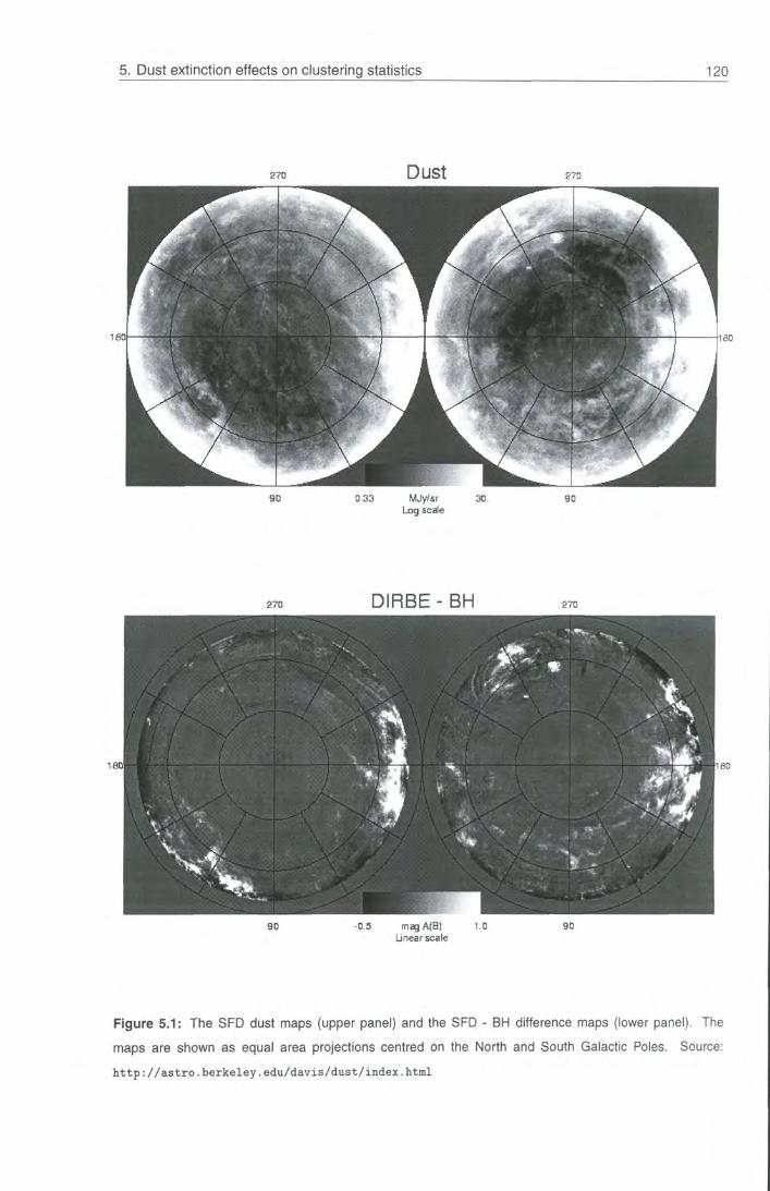
5. Dust extinction effects on clustering statistics 120
leoi
270 Dust 27C
90 D.33 MJylsr 30. Log scale
16D
90
270 DIRBE- BH 270
18DI
90 -0.5 magA(B) Linear scale
1.0 90
160
Figure 5.1: The SFD dust maps (upper panel) and the SFD - BH difference maps (lower panel). The
maps are shown as equal area projections centred on the North and South Galactic Poles. Source:
h t t p : / / a s t r o . b e r k e l e y . e d u / d a v i s / d u s t / i n d e x . h t m l

5. Dust extinction effects on clustering statistics 121
maps is clearly visible, as are the differences at low galactic latitudes and the appearance of large patches nearer the poles with slightly discrepant values.
The real SDSS project will be using the SFD maps to correct the catalogue for dust as
it goes along. So, for us to look at the effects on clustering statistics of a catalogue that
contains dust but has no corrections is a needlessly pessimistic task. A more realistic
target would be to examine a catalogue that is only dust-affected at the level of the errors
in the SFD work. But the errors are of course highly systematic and coherent over the
sky, so in order to get an idea of the errors involved we take the difference between these
maps and those presented in BH. This approach will then give some sort of worst case
indication of the systematics that could be present.
5.3.2 Application to mock catalogues
In order to apply dust to the mock SDSS catalogue, we use the same scheme for as
signing random magnitudes as we do for the "clean" catalogues. We then determine
the angular position of each galaxy in Galactic coordinates, and use the SFD maps to
calculate its EB-V extinction.
The SDSS will select galaxies from photometry in the r ' -band. To correct the magnitude
of the galaxy, we apply the relation (Schlegel, Finkbeiner, & Davis 1998, table 6)
A ' = 2.751EB-V- (5.3)
To perform the equivalent magnitude correction for a 2dF catalogue we would use a
factor of 4.035, which reflects the larger extinction in the shorter wavelength 6j-band used
to select galaxies in the parent APM survey
We note that a zero point in the extinction can have no effect on the clustering signal,
so we subtract the SFD baseline of 0.020 mag in EB-V before applying the correction.
Having obtained the magnitude change, we add it to the magnitude of the galaxy and
throw the galaxy out of the survey if it is fainter than the magnitude limit. We also use
the increased magnitude to lower the value of dmax. the furthest distance that the galaxy
could be seen at before it passes out of the apparent magnitude limit.
The luminosity function of this catalogue was chosen (Chapter 4) to obtain a reasonable
match to galaxy number counts. Changing the galaxy magnitudes to account for redden-

5. Dust extinction effects on clustering statistics 122
ing has the effect of manipulating the selection function. We choose to compensate for this effect by boosting the number density of galaxies, in order to keep the total number of galaxies constant. To keep iVgai « 900,000 we increase by 8.6%. We note that the number counts, dN/dm, will not be the same as for the clean mock catalogues.
For the "corrected" mocks, we subtract the Burstein & Heiles (1982) reddening from
the SFD reddening and add the corresponding magnitude change to the magnitude of
the galaxy. This time, of course, there is potential for objects to be moved to brighter
magnitudes. Since we want to avoid the potential for objects outside the original cata
logue to be scattered into it, we have chosen to add the SFD zero-point, again noting
that it cannot affect the clustering signal at all. Since the two maps are, in general, well
correlated, the differences between them are normally quite small, and this magnitude
shift should be enough to catch all the galaxies. This time, we need to increase by
6.4% to conserve the number of galaxies.
We will thus end up with three mock SDSS catalogues: a "clean" one with no dust, or,
equivalently, perfect dust correction; a "dusty" one; and a "corrected" one.
In figure 5.2 we show the resultant distribution of magnitude shifts in the corrected and
uncorrected maps. As expected, the SFD correction now has a baseline of zero, and the
SFD-BH peaks at 0.02 mag since the majority of galaxies have little correction except for
the 0.02 mag zero point after applying an SFD magnitude shift and then correcting with
BH. It can also be seen that very few galaxies have negative extinction in the corrected
catalogue, so we can be reasonably sure that we are not significantly biased by failing
to catch galaxies that would be scattered in to the tail-end of the magnitude distribution.
This problem could certainly be eliminated altogether by increasing the offset by another
0.03 mag.
5.4 Results: systematic effects on clustering
Our chief interest in dust in this work involves possible bias in the measured clustering
properties of the galaxy distribution caused by observing the galaxies through a dust layer
that has its own correlations.
To assess the effect of dust, we look at three statistics: the power spectrum of a volume
limited sample of galaxies selected from the full SDSS; the power spectrum of the whole.

5. Dust extinction effects on clustering statistics 123
3 x 1 0 5
2 x 1 0 5
105
-1 I 1 I I I I I I I I I I I I I I r
- 0 . 0 5
1 1 1 r
0.05
I L _ _
0.1 0 .15 0.2
Figure 5.2: Histogram of extinction, Eb-v, for galaxies in the dusty sample (dashed line) and corrected
sample (solid line).
magnitude limited SDSS catalogue; and the angular correlation function of the whole
catalogue.
For each statistic, we examine the clean catalogue with no dust effects, the dusty
catalogue with SFD dust and no correction, and the corrected catalogue with SFD dust
and BH correction, as described in 5.3.
In order to measure the power spectrum, we must create a catalogue of random
galaxies with the same window function and density distribution as the catalogue we are

5. Dust extinction effects on clustering statistics 124
measuring. Constructing this catalogue is trivial in the clean case as it simply involves the n{z) function used in the creation of the original mock catalogue. In the dusty and corrected mocks, this n{z) is no longer that which would be measured from the survey since we have thrown galaxies out of the sample. In order to create realistic random catalogues for these realizations, we take galaxies from the distribution before throwing them out due to dust effects, and for each galaxy pick a random line of sight that is within the angular bounds of the SDSS window function. We then change the magnitude of the galaxy according to the amount of extinction along this random direction. In this way we model the correct distribution of reddening without introducing any correlations into the random catalogue.
5.4.1 The power spectrum - volume limited case
In the case of a volume limited sample of galaxies without dust, we are simply selecting a
constant density wedge from the galaxy catalogue out to a fixed radius. Introducing dust
has the effect of changing the dmax values of the galaxies, so, galaxies near the volume
limit are scattered in and out of the sample. Effectively then, we still have a wedge but
its furthest edge is now ragged due to the different magnitude shifts along different lines
of sight. Our technique for constructing the random catalogue with no clustering means
that the edge of the random catalogue is at the average distance of galaxies at the edge
of the real catalogue, but it still has a sharp cut-off with distance. A systematic bias will
be introduced since the real and random catalogues do not have the same shape. If
the dust has a characteristic clustering scale, 6c, then we would expect to see biases in
the power spectrum on scales of around r6c, where r is the depth of the survey In the
example shown here, we use a volume limit of z = 0.23, which translates to a comoving
distance r = 590h~^ Mpc. For the fast Fourier transform analysis, we use a box size of
1036.8/i~^ Mpc, three times the length of the simulation, and a 192 grid. We show results
for the effect of dust on the power spectrum in figure 5.3. There is a large systematic
problem with the dusty, uncorrected catalogue in the very long wavelength regime, in
excess of the random errors associated with these points. It would therefore seem that
failing to correct the SDSS redshift survey for dust extinction effects would result in a
strong bias in measurements of large-scale power, entirely removing the turn-over we
would expect to see in a CDM-type model.
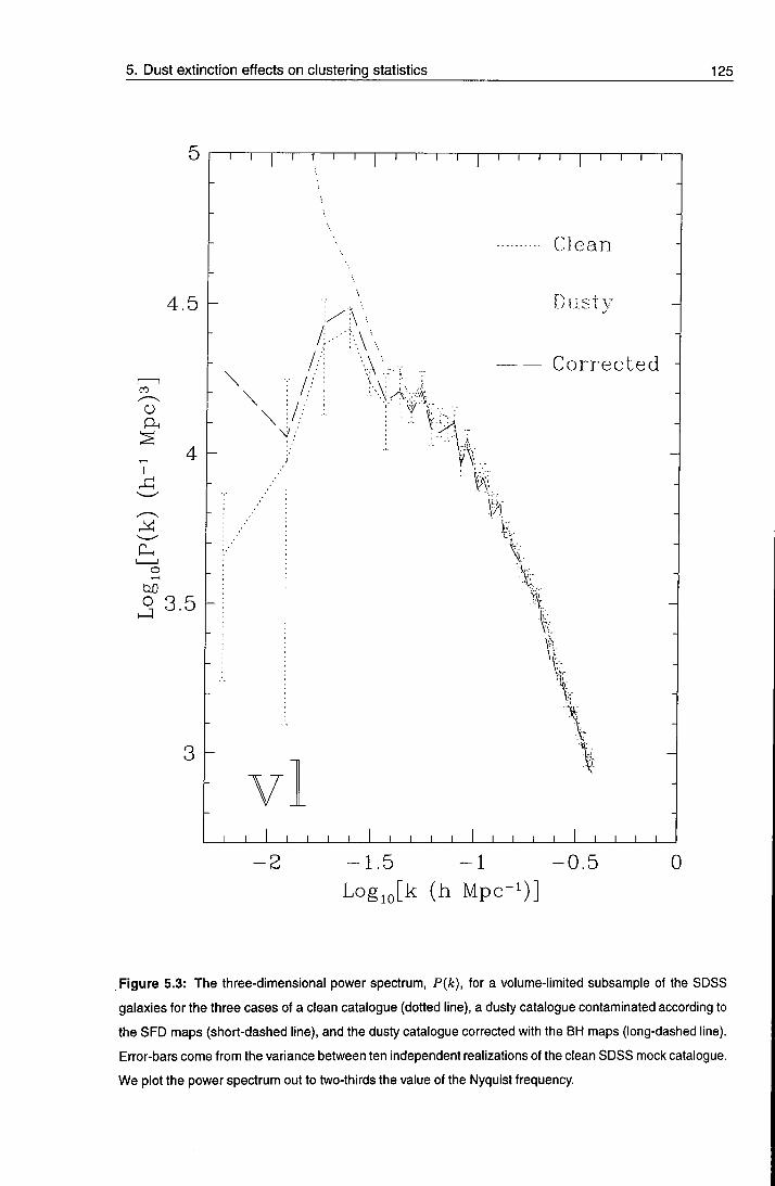
5. Dust extinction effects on clustering statistics 125
4.5
o
I
" I — r n — 1 — I — r T — I — I — r n I I r - I — I — I — r
/
Clean
Dusty
Corrected
9 3.5
ft
% \
I . •1
J L J I I I J I I L J I L
- 1 . 5 -1 - 0 . 5 L o g j j k (h Mpc-O;
0
Figure 5.3: The three-dimensional power spectrum, P{k), for a volume-limited subsample of the SDSS
galaxies for the three cases of a clean catalogue (dotted line), a dusty catalogue contaminated according to
the SFD maps (short-dashed line), and the dusty catalogue corrected with the BH maps (long-dashed line).
Error-bars come from the variance between ten independent realizations of the clean SDSS mock catalogue.
We plot the power spectrum out to two-thirds the value of the Nyquist frequency

5. Dust extinction effects on clustering statistics 126
5.4.2 The power spectrum - magnitude limited case
For the case of the whole, magnitude limited sample, the same reasoning applies, except
that a dust fluctuation on a certain angular scale has an effect on the density along that
line of sight for the entire depth of the survey Thus dust can introduce a bias between the
real and random catalogues at smaller physical scales than in the volume limited case.
We weight the galaxy sample with the FKP minimum variance weighting method, as
described in Chapter 3, with P = A000h~^ Mpc . As with the volume limited case, the
analysis is performed on a 192 grid with length 1036.8/i"^ Mpc.
In figure 5.4 we show results for the three-dimensional power spectrum in the case of
the clean, dusty and corrected catalogues. As in the volume limited case, the corrected
catalogue seems to recover the power extremely well out to large scales, whereas the
uncorrected catalogue has significantly higher amplitude in this regime: well outside the
range allowed by random errors on the power spectrum.
5.4.3 The angular correlation function,w{9)
The angular correlation function is a measure of the amplitude of clustering of objects
on the sky as a function of angular separation, 9, and as such we expect it to be more
sensitive to contamination by dust, which itself has power only in an angular sense. The
angular correlation function carries less information than its 3D counterpart, since one
dimension is projected out, so to calculate w{6) for a redshift survey is rather a perverse
use of the data. However, the SDSS survey will consist of an angular catalogue of 10
galaxies, of which the redshift survey is a subset. The survey then, will provide extremely
accurate data due to its high sampling rate, and we can use the mock SDSS to assess
the systematic error introduced by failing to correct for dust or by plausible errors in the
SFD dust-correction technique.
In figures 5.5, 5.6 and 5.7, we plot the angular correlation function from the mock SDSS
catalogue with no dust, SFD dust and SFD-BH corrected dust, respectively
In order to save computational time, we split the sample up Into ten different apparent
magnitude bins and calculate the correlation function for each one individually Rather
than applying fixed bounds on the magnitude range for each bin, we choose Am such

5. Dust extinction effects on clustering statistics 127
4.5
o Ph
I
I I
o 1—1
4
1—r n — r "1 r n — I — I — r n I I r
0 3.5
4
C.lea.n
Diistv
/ : / / ^ I l k
Corrected
J L J I I L J L J \ L J I I L
- 2 - 1 . 5 -1 - 0 . 5 Log^Jk (h Mpc-^;
0
Figure 5.4: As for figure 5.3 but this time the galaxies are the whole, flux limited SDSS sample weighted
with an FKP scheme, as described in section 5.4.2.

5. Dust extinction effects on clustering statistics 128
0
Clean
m o
- 2
x#>g^ N.
J I I L
•. > x X
Vv : ; . \^ i X
' • \ '•'}• '
J I I I t l i U L
-1 0 1 Logio [^(degrees);
Figure 5.5: The angular correlation function, w{d) for our SDSS mocl< catalogue with fio = 1, Ao = 0. The
dotted lines show w(9) for ten different magnitude bins out to the limiting SDSS magnitude, whilst the dots
show the correlation function scaled using the relation described in section 5.4.3. The dashed line shows
the average over the ten magnitude slices.

5. Dust extinction effects on clustering statistics 129
0
n I I r 1 I 1 r
!3usty V
-
O
- 3
V-/X \
-| r
J L J I L
-1 0 Logio [^(degrees);
Figure 5.6: As for figure 5.5 but the correlation function is for the mock catalogue with dust Introduced via
the SFD dust maps.

5. Dust extinction effects on clustering statistics 130
0
~i r n r — — r 1 1 1 r n r
\ x\
; V x \^
'•• x ,f , , x ^ -
Correctec.
CD
O
- 2
xSfx>>..,
J L
X )N>!«
- 'V- ••• ^ '•-.••A\;,
; x \ ,
; \
J I I L J I I L I " l I
1 0 Logio [^(degrees);
Figure 5.7: As figures 5.5 and 5.6, but this time the correlations are for dust that has been added using the
SFD maps, and corrected for using the BH maps.
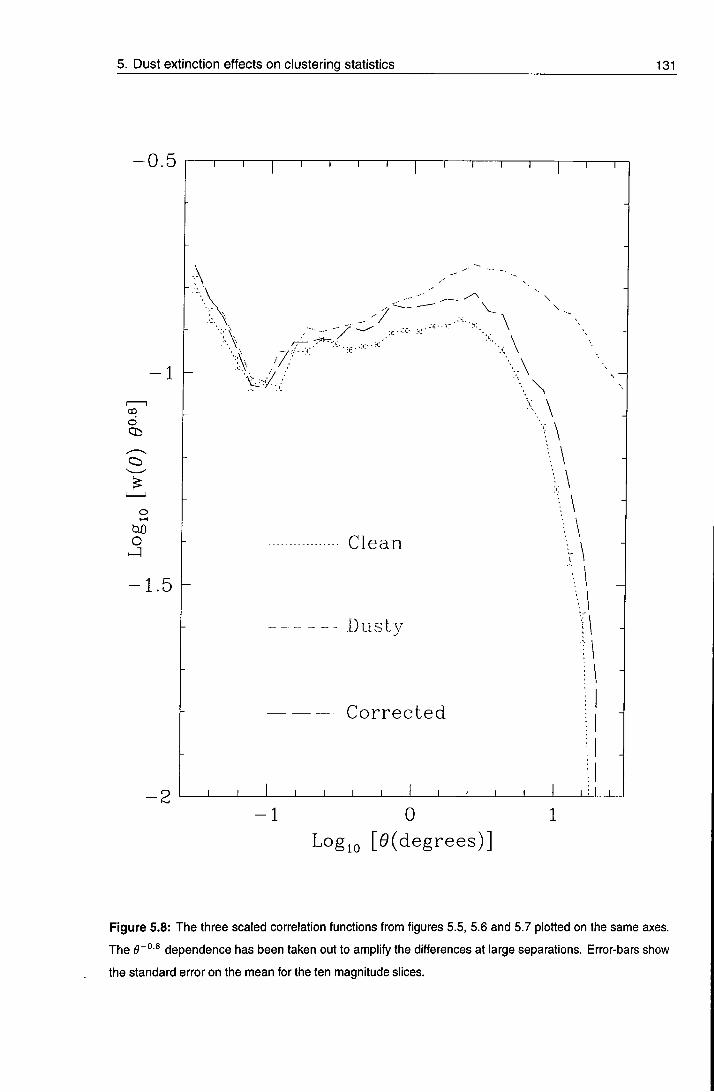
5. Dust extinction effects on clustering statistics 131
0.5
CO
d
CI5
o
~i r n i 1 r
- 1 . 5
- 2 J L
Clean
Dusiv
T 1 r n r
\ ••x \
'••v\
Correc ted
J I I L I I I
\
w v \
U W
1 0 1 Logio [^(degrees);
Figure 5.8: The three scaled correlation functions from figures 5.5, 5.6 and 5.7 plotted on the same axes.
The * dependence has been taken out to amplify the differences at large separations. Error-bars show
the standard error on the mean for the ten magnitude slices.

5. Dust extinction effects on clustering statistics 132
O
"1 r T r 1 1 1 r
I
- 2
4
11 T
' H i / , I - 1 , 1 1 I
I 1 -1 V
"I r
^ - T
1 J 1 I L I I I
-1 0 Logio [^(degrees);
Figure 5.9: The correlation function of the SFD dust map (dotted line) and the SFD-BH difference map
(dashed line). As explained in the text, we obtain the correlation function of the dust by subtracting the
'dusty' correlation function from that of the dust-free catalogue. The vertical, long-dashed lines give the
angular resolution of the SFD maps (0.1°) and the BH maps (0.6°).

5. Dust extinction effects on clustering statistics 133
that each of the ten samples has a similar number of objects in it, this method being the
most efficient use of resources.
The correlation function is expected to obey a simple scaling relation, where the angular
scale and the amplitude are proportional to the inverse of D^,, which is the distance at
which an L* galaxy would have magnitude equal to the limiting magnitude of the bin.
Hence,
(Peebles 1993). Given that magnitude, m, is equal to 2.5log/, it can be seen that
oc 10-"'/^ (5.5)
This relation provides an easy method for comparing the angular correlation function in
different magnitude bins.
Table 5.1. Limiting magnitudes for our ten magnitude bins and the corresponding values of D^,, the charac
teristic depth, as a fraction of the characteristic depth of the brightest (nearest) bin.
Limiting magnitude
17.07 1
17.61 0.7798
17.93 0.6730
18.16 0.6053
18.34 0.5572
18.49 0.5200
18.61 0.4920
18.72 0.4677
18.82 0.4467
18.90 0.4305
In table 5.1 we present the limiting magnitudes and corresponding relative values of D^,
for the ten magnitude bins. In figures 5.5, 5.6 and 5.7 we plot as crosses the measured

5. Dust extinction effects on clustering statistics 134
values of the correlation function scaled up by the correct factor. The dashed line is the average over the ten different bins. It can be seen that the scaling relation works extremely well for the mock catalogues. There is a high level of scatter (indicated by the spread of the dots) in the relation for large 6 in the dusty catalogue; this scatter is not random noise but rather exists because the dust distribution that contaminates the background signal has no scaling relation, but instead has a fixed scale length independent of the galaxies being observed.
It can be seen from these figures that the presence of underlying correlations in the
foreground can strongly contaminate the galaxy clustering signal, resulting in an observed
angular correlation function that is systematically biased. In figure 5.8 we plot the average
curves from the previous three figures, ie. the correctly scaled angular correlation function
for the clean, dusty and corrected catalogues. To enhance the difference between the
curves on large scales, we divide w{6) by the canonical dependence of the correlation
function, w{e) oc (Groth & Peebles 1977). The error-bars show the standard error
on the mean from the ten magnitude slices after scaling to the same effective depth. It
can clearly be seen that the dusty catalogue is biased to a highly significant level on all
scales above 0.2°. The clustering in the dust distribution has the effect of adding a lot of
power on these scales. The corrected catalogue is much healthier, with its shape much
more similar to that of the clean catalogue, but comparison with the error-bars shows that
it is still significantly biased compared to the level of random uncertainty in the measured
w{e). Since the ten slices occupy overlapping volumes, they are in fact rather correlated,
and these error-bars reflect a certain underestimation of the true error. However, even in
a worst-case scenario where we plot the standard deviation of the ten slices, rather than
the error on the mean, the corrected line is biased at the l-a level for 9 > 0.3°.
Perhaps a more illustrative picture of the effect of dust comes if we subtract the clus
tering signal due to correlations in the background galaxy distribution. The observed
correlation function is given by
Wohs = WdustWg^l + ^^dust + 'Wga.l, (5.6)
assuming that the foreground and background distributions are entirely uncorrelated (see
Geller, De Lapparent, & Kurtz 1984, although their application of this method is to study

5. Dust extinction effects on clustering statistics 135
correlations between plates). Thus we derive an expression for the correlation function of the dust,
1 + tOgal
This function is plotted In 5.9 for the case of no dust-correction and for correction via the
BH maps. The plots are averaged over the ten magnitude bins, although in this case
note that the above scaling relation has not be applied since the dust has fixed angular
and physical clustering properties, independent of the depth of the survey. The error bars
come from the variances between the different magnitude samples, which are of course
not statistically independent, so they will tend to underestimate the true error on w^ust-
Three distinct regimes can be identified from this graph:
1 . Very noisy signal at small separations. We expect to see no clustering for small
angular separations since the //?/4S-derived SFD maps have angular resolution ~ 6',
so there is no real information about clustering on scales below this ( l o g ^ ^ - 1 ) . In
fact we see a very noisy signal on these scales because the number of very close
pairs is small.
2. Similar correlations on intermediate scales. Around ^ = 1° both correlation func
tions are at a similar level. The H i survey (Heiles 1975) used to compile the BH dust
maps has a beam width of 0 .6° , so in this regime we are between the angular reso
lution of the two maps. The small scale power, then, in both cases comes only from
the SFD maps, and we should thus expect little difference in the angular correlation
function on these scales.
3. Long wavelengths. For large separations, the BH correction is doing a good job of re
moving the dust contamination from the SFD maps, and even this worst case scenario
view of systematic errors leads to leads to an order of magnitude less contamination
of the intrinsic clustering signal at ^ « 10° .
5.5 Conclusions
In this chapter we have shown that, on small scales, dust is of little significance in the
clustering statistics. Its most crucial effect is that of altering the power spectrum on large

5. Dust extinction effects on clustering statistics 136
spatial scales. Unfortunately, the dust power appears to affect the power spectrum in both
the volume and magnitude limited cases at around the scale where we would expect to
see the turnover in CDM-variant models. This coincidence is extremely irksome since
the turnover is one of the key predictions of such models, and its precise location is an
important parameter. Currently we do not really know precisely how accurate the SFD
recipe is, and we must stress that using the SFD-BH difference maps could lead to an
over-prediction in the level of systematic error. However, it is apparent from this work that
estimates of the shape parameter from the SDSS power spectrum could be significantly
biased, even once dust has been corrected for to the best of our current ability.
Failing to correct for dust at all can obviously produce very high biases in measurements
of large-scale power, and we speculate that recent work (Sylos Labini & Montuori 1998)
claiming to see no evidence for a turnover to homogeneity in large galaxy samples like the
Stromlo-APM redshift catalogue could be mistaking fluctuations in the dust distribution in
our Galaxy for fractal clustering patterns in the large-scale structure of the Universe.
We intend to apply the SFD dust maps to the APM-selected galaxy catalogues, and
hence investigate the likely effect on clustering in the Stromlo-APM and 2dF surveys.
The effect is likely to be even more pronounced than for the SDSS, since the magnitude
correction per unit of extinction is 5 0 % higher (section 5.3.2). For the 2dF this will be
countered by the fact that the South Galactic strip is located in a region of very low
extinction, whereas the SDSS goes down to quite low galactic latitudes, where there is
significant contamination.
The rest of the work in this thesis concerns estimation of the ^-parameter ^o^/b)
from redshift-space distortions to the power spectrum. We have shown that the power
spectrum itself can be quite seriously contaminated by dust, but it will be interesting to
investigate whether the magnitude of the measured anisotropy is more or less robust to
dust extinction effects.
References
Boulanger R, Perault M., 1988, ApJ, 330, 964
Burstein D., Heiles C, 1978, ApJ, 225, 40
Burstein D., Heiles C, 1982, AJ, 87, 1165
Burstein D., McDonald L. H., 1975, AJ, 80,17
FaberS. M., 1973, ApJ, 179, 731

5. Dust extinction effects on clustering statistics 137
Geller M. J., De Lapparent V., Kurtz M. J., 1984, ApJ Lett, 287, L55 Groth E. J., Peebles P. J. E., 1977, ApJ, 217, 385 Helles C, 1975, A&A Supp, 20, 37 Heiles C, 1976, ApJ, 204, 379
Hilditch R. W., Hill G., Barnes J. V., 1976, MNRAS, 176,175
Nichol R. C, Collins C. A., 1993, MNRAS, 265, 867
Peebles P. J. E., 1993, Principles of Physical Cosmology. Princeton University Press, Princeton
Schlegel D. J., Finkbeiner D. R, Davis M., 1998, ApJ, 500, 525
Shane C. D., Wirtanen C. A., 1967, Pub. Lick Obs., 22,1
Stark A. A., Gammie C. R, Wilson R. W., Bally J., Linke R. A., Heiles C, Hunwitz M., 1992, ApJ Supp, 79,
77
Sylos Labini R, Montuori M., 1998, A&A, 331, 809
Trumpler R. J., 1930, Lick Observatory Bulletin, 420,154
Wheelock S. L. et al., 1994, IRAS sky survey atlas: Explanatory supplement. JPL publication 94-11
Chapter 6
Redshift-space distortions
THE ARGUMENT. We use a set of large, high-resolution cosmological A/-body
simulations to examine the redshift-space distortions of galaxy clustering on
scales of order W-200h~^ Mpc. Galaxy redshift surveys currently in progress
will, on completion, allow us to measure the quadrupole distortion in the 2-
point correlation function, ^{a, TT), or its Fourier transform, the power spectrum,
P(fe,/i), to a high degree of accuracy. On these scales we typically find a
positive quadrupole, as expected for coherent infall onto overdense regions
and outflow from underdense regions, but the distortion Is substantially weaker
than that predicted by pure linear theory. We assess two models that may be
regarded as refinements to linear theory, the Zel'dovich approximation and a
velocity dispersion model. We find that neither provides an adequate physical
description of the clustering pattern. If used to model redshift-space distortions
on scales for 10 < A < 200 / i " ' Mpc the estimated value o1 P {P = f(^o)/b
where / ( f i o ) ~ and 6 is the galaxy bias parameter) is liable to systematic
errors of order ten per cent or more. We discuss how such systematics can
be avoided by i) development of a more complete model of redshift distortions
and ii) the direct use of galaxy catalogues generated from non-linear W-body
simulations.
6.1 Introduction
In early galaxy redshift surveys (Jackson 1972; Gregory & Thompson 1978), some of
the most striking artefacts observed were the so-called "fingers of God": ridges in the
galaxy distribution pointing directly at the observer. The first evidence of the redshift-
space distortion of galaxy clustering had been observed. If galaxy motions were perfectly
described by the Hubble flow, then redshift would be an accurate indicator of distance,
and the clustering pattern observed in redshift surveys would be statistically isotropic.

6. Redshift-space distortions 139
Peculiar velocities perturb the redshifts, and hence the inferred distances, of the galaxies,
generating the observed anisotropic clustering pattern.
Real Redshift
line of sight
Figure 6.1: Qualitative picture of redshift space distortions. On the top is a linear perturbation, a galaxy
cluster whose mass exerts gravitational force on nearby objects causing a collapse. Thus the cluster appears
collapsed along the line of sight when viewed in redshift-space. On the bottom we show the non-linear case
of a collapsed cluster whose members have thermal velocities. The cluster is smeared out along the line of
sight when viewed in redshift-space.
Galaxy peculiar velocities can arise as a local effect, when the non-linear velocities of
virialized groups and clusters create the fingers of God by stretching out these structures
along the line of sight. On large scales, the clustering pattern is predicted (as suggested
in Sargent & Turner 1977) to be compressed along the line of sight by coherent infall onto
galaxy clusters and super-clusters, and outflow from voids and other underdense regions.
Figure 6.1 is a simple representation of these two regimes and their effect on isotropy
On both scales, the anisotropy of galaxy clustering encodes information about the
galaxy velocity field and hence the underlying mass density field that gave rise to it.
Measurements of redshift-space distortions can therefore be used to place constraints
on the density parameter, QQ, and the bias parameter, b, which relates fluctuations in the
galaxy distribution to those in the mass distribution. A comprehensive review of linear
redshift-space distortions can be found in Hamilton (1997).

6. Redshift-space distortions 140
Redshift-space distortions directly measure the combination of parameters /? = Og- is approximately the logarithmic derivative of the linear growth factor with respect to the expansion factor, and so relates particle velocities to the gradient of the mass distribution. is thus the factor that relates particle velocities to the gradient of the galaxy overdensity field. Interesting constraints on this quantity have been obtained by analysis of optical redshift surveys (Loveday et al. 1996; Ratcliffe et al. 1998a) and IRAS surveys (eg. Hamilton 1993; Fisher et al. 1994; Cole, Fisher, & Weinberg 1995 and more recent papers such as Fisher & Nusser 1996; Bromley Warren, & Zurek 1997). However, the statistical errors remain large and no consensus on the value of (3 has been reached (for a review see Strauss & Willick 1996). The next generation of large surveys, including the 2-degree-Field (2dF Colless 1995) and Sloan Digital Sky Survey (SDSS, Gunn & Weinberg 1995), will enable redshift-space distortions to be measured with unprecedented accuracy These surveys should allow p to be measured to an accuracy of better than 1 0 % (see Chapters 7 and 8), and possibly for CIQ and b to be separately constrained. To achieve such accuracy and avoid systematic errors it is important that the theoretical modelling of redshift-space distortions be accurate. This is a non-trivial requirement, as these surveys will provide their most precise measurements of the distortions on scales of 3 0 - 1 0 0 / i " ^ M p c , where the predictions of pure linear theory are not expected to hold exactly
In this chapter we investigate the usefulness of existing models for the distortions
using a set of high-resolution N-hody simulations. These simulations accurately follow
the evolution of clustering over the range of scales that will be probed by the next-
generation surveys. Our aim is not to formulate a procedure for analysing real data, and
so, rather than constructing mock galaxy catalogues, we instead use the full simulations
to quantify the redshift-space distortions as accurately as possible. We thus assess
the accuracy of the linear theory model and two proposed extensions to it. We make
no attempt to examine the cosmological anisotropies that occur when the cosmological
model adopted to map distance to redshift does not have the true values of fio or AQ
(Matsubara & Suto 1996; Ballinger, Peacock, & Heavens 1996). Neither do we investi
gate the validity of the "distant observer" approximation, which assumes that the scales
of interest in the survey subtend a small angle at the observer.

6. Redshift-space distortions 141
In section 6.2 we define our notation convention and introduce the quadrupole statistic used to assess the level of redshift-space distortion. Section 6.3 details the parameters of the set of A/-body simulations, and explains the methods we employ to construct biased galaxy samples. The linear theory prediction and the two other models are described in section 6.4. In section 6.5 we compare the analytic models with measurements of the redshift-space distortions in the AZ-body simulations. We discuss results in section 6.6.
6.2 Anisotropy in redshift-space
6.2.1 The power spectrum
Our method of analysis uses the power spectrum, P(k) , which is the Fourier transform of
the correlation function,
P(k) = lar)e'^-'d\ (6.1)
where we use the Fourier convention that the wavenumber, k, is the angular frequency
corresponding to wavelength A, ie. k = 27r/A. The correlation function is given by
e(r) = (<5(x + r)^(x)), (6.2)
where ^(r) is the fractional overdensity,
S{r) = (6.3)
The power spectrum has been used by many authors to study the growth of grav
itational clustering in simulations, and to quantify the clustering observed in red-
shift surveys (for recent examples, see da Costa etal . 1994; Tadros & Efstathiou 1995;
Shectman eta l . 1996).
When galaxy distances are measured in redshift space, their peculiar velocities (ie.
relative to the pure Hubble flow) distort the pattern of galaxy clustering by displacing
galaxy positions along the line of sight. Thus a galaxy whose true position is r appears
in redshift space at the position:
s = r -f J7(r)f, (6.4)

6. Redshift-space distortions 142
where the line-of-slght peculiar velocity U{r) = v(r) . f . Here we have adopted units in which the Hubble constant has unit value; distance is measured in units of M p c , where h = £ r o / ( 1 0 0 k m s ~ ^ M p c ~ ^ ) , and velocities in units of l O O k m s " ^
In redshift space this displacement in a preferred direction causes the observed power
spectrum to be anisotropic, with different values for wavevectors along the line of sight to
those perpendicular to it. Thus, the redshift-space power spectrum can be thought of as
a function of k (= |k|) and n, the cosine of the angle between wavevector k and the line
of sight,
Pik) = P{k,fi). (6.5)
We use the convention that P(k) or P{k, n) refers to the redshift-space power spectrum,
since this quantity depends on both the magnitude and direction of k, whereas P{k)
represents the real-space power spectrum, depending only on the scalar k.
6.2.2 The quadrupole ratio
The redshift-space distortions can be conveniently quantified by a simple statistic. The
anisotropy in P(k ) is symmetric in /x, ie. P{k,n) = P{k, -n), so the distortion depends
only on even powers of n. To measure the extent of deformation from isotropy we
decompose the power spectrum into multipole moments using the Legendre polynomials,
Li{fj,). Thus,
oo P{k,fi) = ^Piik)Li{i,), (6.6)
1=0
where the sum is over even values of /. From the orthogonality relation for Legendre
Polynomials, the multipole moments Pi{k) can be found by evaluating
Piik) = £^'p(A;,/z)LKM)d/i- (6.7)
We find that estimates of Pi{k) rapidly become noisy for multipoles with / > 2, so we
choose to use as the key statistic for our analysis the quadrupole to monopole ratio,
P2{k)/Po{k).
We have chosen to carry out all analysis in A;-space using power spectrum multipoles
Pi{k). However, our results can readily be translated into predictions of the multipole
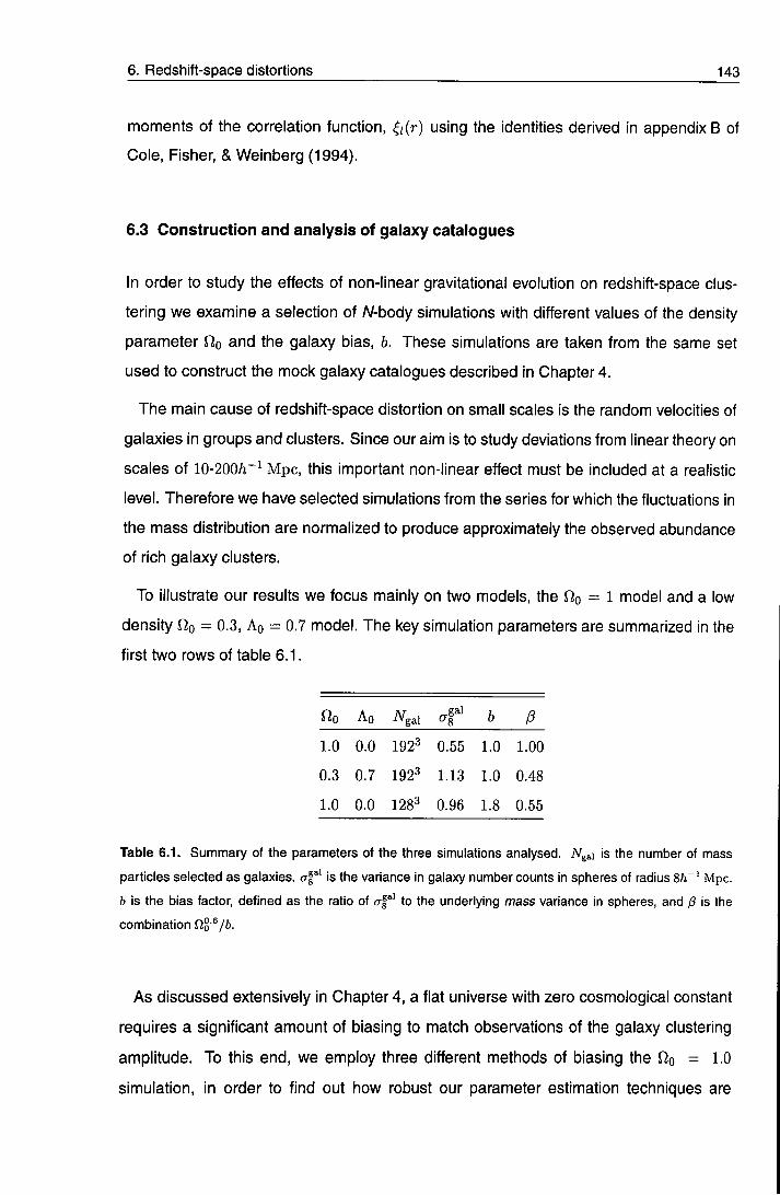
6. Redshift-space distortions 143
moments of the correlation function, ^i{r) using the identities derived in appendix B of
Cole, Fisher, & Weinberg (1994).
6.3 Construction and analysis of galaxy catalogues
In order to study the effects of non-linear gravitational evolution on redshift-space clus
tering we examine a selection of A/-body simulations with different values of the density
parameter QQ and the galaxy bias, b. These simulations are taken from the same set
used to construct the mock galaxy catalogues described in Chapter 4.
The main cause of redshift-space distortion on small scales is the random velocities of
galaxies in groups and clusters. Since our aim is to study deviations from linear theory on
scales of l0-200h~^ M p c , this important non-linear effect must be included at a realistic
level. Therefore we have selected simulations from the series for which the fluctuations in
the mass distribution are normalized to produce approximately the observed abundance
of rich galaxy clusters.
To illustrate our results we focus mainly on two models, the fio = 1 model and a low
density Oo = 0.3, Ao = 0.7 model. The key simulation parameters are summarized in the
first two rows of table 6.1.
no Ao ^8 b
1.0 0.0 192^ 0.55 1.0 1.00
0.3 0.7 192^ 1.13 1.0 0.48
1.0 0.0 128^ 0.96 1.8 0.55
Table 6.1. Summary of the parameters of the three simulations analysed. Ngai is the number of mass
particles selected as galaxies, o-f*' is the variance in galaxy number counts in spheres of radius 8/i"' Mpc.
b is the bias factor, defined as the ratio of af*' to the underlying mass variance in spheres, and 0 is the
combination Qo^/b.
As discussed extensively in Chapter 4, a flat universe with zero cosmological constant
requires a significant amount of biasing to match observations of the galaxy clustering
amplitude. To this end, we employ three different methods of biasing the QQ = 1.0
simulation, in order to find out how robust our parameter estimation techniques are

6. Redshift-space distortions 144
^ 2
1 1 1 1 1 1 1 1 1 1 1 1 1 1 1 1 1 1 1 j 1 1
n„=i.o,A„=o.o
- --^-X-^^ n„=0.3,A„=0.7 \ ^
- \ \ NX
- \ \ \ \
\ N, _
1 1 1 1 1 1
v s . ^
\ \ \
\ \ \ ^
1 1 1 I 1 1 1 1 1 1 1 1 1 1 l \ l
- 2 - 1 . 5 - 1 - 0 . 5 0 l o g J k / h M p c - 0
Figure 6.2: Power spectra of the real-space mass distributions of the A/-body simulations described in
section 6.3. In each case the thin line is the linear theory, r = 0.25 CDM spectrum (equation 4.1) which was
used to set up the initial conditions of the simulations, extrapolated to the present day, and the thicker line is
the evolved, non-linear power spectrum of the simulation measured at z = 0.
to the precise bias prescription. The methods used are similar to those described
in Chapter 4, assigning selection probabilities to dark matter particles based on the
value of the local mean density. In each case the bias is chosen to obtain a a f^ ' , the
variance in galaxy counts in spheres of radius 8h~^ M p c , consistent with the results
of Maddox, Efstathiou, & Sutherland (1996), who find a f ' = 0.96 for the APM Galaxy
Survey. Thus, the bias factor, defined as c r f ^ ' / ' ^s . has value 6 = 1.81. The parameters of
our biased simulation are given in the third row of table 6.1. The three methods used are:
• High Peaks. We bias the dark matter distribution with a high peaks model, as de
scribed in Chapter 4, section 4.4, model 3.
• Exponential. This model is a variant on the Lagrangian exponential model described
in section 4.4, model 1. Since we only need to bias one simulation, with a moderate
degree of bias, we use the same technique with a simpler form of the probability
formula:
P{u) = A exp(az^ -t- /3u\v\). (6.8)

6. Redshift-space distortions 145
• Threshold. This model is, again, as described in section 4.4, model 4. The particle distribution resulting from this scheme is expected to contain large voids since the sharp cut-off at the threshold is extremely effective at evacuating underdense regions (Weinberg & Cole 1992).
The three methods described here are intended to span a broad range of plausible
biasing prescnptions that might occur in the real universe. If so, and if we can develop
techniques that are unaffected by the choice of scheme, these techniques should be
insensitive to the way in which bias really comes about.
The density of the biased catalogues is chosen to be one galaxy per 25(/i~^ M p c ) ^
volume, roughly four times 0*, the observed number density of L * galaxies (eg.
Peebles 1993, §5; Ratcliffe eta l . 1998b). The high sampling density has been adopted
as we are interested in investigating systematic effects on the redshift-space distortions,
and so want to minimize the statistical uncertainties produced by sparse sampling.
6.3.1 Zel'dovich approximation simulations
In section 6.5 we will compare the redshift-space distortions measured in the A/-body
simulations with a similar analysis of Monte Carlo implementations of the Zel'dovich
approximation. Our Monte Carlo realizations have the same 192^ particle grid and initial
density field parameters as the corresponding A/-body simulations. Exactly the same
method is used to perturb the particles as that employed to set the initial displacements
in the A/-body simulation, only with a much larger perturbation amplitude corresponding
to ; = 0 rather than the starting redshift of the simulation. For the A/-body simulations
we populate all the modes in the 192^ fc-space grid including those in the corners of the
cube. However for these realizations of the ZA, we make our treatment consistent with
the analytic calculation that we outline in section 6.4.2, by smoothing the density field in
the same way ie. by truncating the power spectrum isotropically at the Nyquist frequency
of the grid, AiNyq = 27r/2Lceii, where Lceii is the length of one grid cell.
These realizations of the ZA can be biased using exactly the same prescriptions that
we use for the N-hody simulations. The catalogues thus created are then subjected to
the same multipole analysis as our A/-body simulations.

6. Redshift-space distortions 146
6.3.2 Estimation of multipole moments
We ensure that the distant observer approximation is satisfied by assigning redshift-space
positions to galaxies based on their distance along the x-ax\s of the simulation. Effectively
the simulation box is placed at infinity and the line of sight aligned with the x-axis. To
minimise the noise in our estimates we repeat the analysis with the simulation rotated to
align the line of sight with the y- and then 2r-axes and average the results.
We use a fast Fourier transform (FFT) analysis with a cloud-in-cell (CIC) assignment
scheme to obtain the power spectrum from the particle distribution, as described in
Chapter 3.
For the biased galaxy simulations a constant equal to the inverse of the number density
of galaxies in the catalogue is subtracted at this point to account for the shot noise
introduced by the Poisson sampling of the galaxies. This correction is not necessary
in the unbiased cases as here we use all the particles from the original glass distribution
rather than a Poisson sample.
The multipole moments of the power spectrum are estimated by approximating the
integral of in equation 6.7 by a discrete sum over modes. This method works perfectly
well at high-A;, but for the first few shells, where the sampling of A;-space results in poor
sampling in / i , it leads to a small systematic error in P2{k)/Po{k). An alternative method of
estimating P2{k) and Po(^). which can readily be employed for low-A;, is to make a least
squares fit to the fj, dependence of P{k, n) using a basis of the Legendre polynomials
Lo,L2 and L4. This second method produces a less noisy estimator but still suffers from
a small systematic error due to the poor sampling in /x. Empirically we find this error to be
independent of the input power spectrum, and so we choose to correct for it by applying
a small (5% for the lowest wavenumber) correction to our first five bins in k.
The lowest A;-mode probed using this method is the fundamental mode of the box,
kp = 2n/LBox, ie- when one wavelength spans the whole box. The highest is the Nyquist
frequency, A;Nyq - kp x {N/2), where iV is the number of cells along one side of the
simulation box. We do not expect our treatment to work all the way up to the Nyquist
frequency, since the deconvolution correction can never recover all the information lost
by assigning particles to a discrete grid. This effect can be seen in figure 6.2 where

6. Redshift-space distortions 147
the power spectrum turns up for the very highest A;-values. For this reason we limit our
analysis rather conservatively to modes with k < % y q / 2 , as explained in Chapter 3.
6.4 Analytic models
Assuming that the velocity field, v(r), is generated via gravitational instability, it can be
related to the underlying mass density field. Here we consider three analytic models
for the relationship of the velocity field to the density field, which lead to quantitative
descriptions of the redshift-space distortion of galaxy clustering. The first is based purely
on linear theory In the second, the effect of non-linear velocities in galaxy clusters is
modelled by adding a random velocity dispersion to the velocity predicted by linear theory
The magnitude of this dispersion, o-„, is not predicted by the model, but is expected to bear
some relation to the typical thermal velocity of galaxies within groups and clusters. The
third model is the Zel'dovich approximation (ZA) (Zel'dovich 1970). This model provides
a complete description of the evolved density and velocity fields, which is expected to be
accurate in the quasi-linear regime where the overdensity predicted by linear theory is of
order unity. Thus this model has the potential to give an accurate physical description
of redshift-space clustering. These three models are described in detail below and
compared in figure 6.3. In each case we assume that the distant observer approximation
is well satisfied and that we are dealing with volume limited galaxy samples. The effects
of relaxing these assumptions are discussed in Kaiser (1987).
6.4.1 Linear theory
In the regime of linear theory, Kaiser (1987) showed that the redshift-space power spec
trum is related to the real-space power spectrum in a very simple way:
p{k,^J) = P { k ) { l + p ^ ? ) \ p = f{no)/b^niyb. (6.9)
The function / ( f i o ) ~ ^^o^ is the logarithmic derivative of the fluctuation growth rate
(Peebles 1993, §14 ; Bouchetetal. 1995). The bias factor, b, is an assumed constant
relating fluctuations in the galaxy density to those in the mass. We derive this result in
Appendix A. Applying equation 6.7 for the / = 0 and / = 2 modes results in
P2 4 /3 /3 + 4 ^ 2 / 7
Po 1 + 2 / 3 / 3 + /52/5" (6.10)

6. Redshift-space distortions 148
o
0.5
-0.5
- 1
Linear Theory
I I I I I I I Zel'dovich Approx. — Dispersion model n,= i.o
0.4 k / h M p c - '
Figure 6.3: Model predictions for the redshift space power spectrum quadrupole to monopole ratio
P2ik)/Poik). The two sets of curves are for two unbiased (6 = 1) CDM models with r = 0.25 power
spectra. The upper curves are for fio = 1-0, o-g = 0.55, while the lower model is Qo = 0.3, Ao = 0.7 and
era = 1.13. In both cases the curves show the constant ratio predicted by linear theory (dotted), the analytic
Zei'dovich Approximation result (solid), and examples of the dispersion model (dashed) with < 7 „ = SOOkm s~'
for f2o = 1.0 and <T„ = 500kms~' for Qo = 0-3. The error bars are centred on the averages of forty random
Monte Carlo realizations of the Zel'dovich approximation. These error bars indicate the standard deviation
of the sample, and thus are typical of the error expected in a single realization. The analytic Zel'dovich
Approximation curve only extends down to the scale at which our integration technique breaks down, as
explained in section 6.4.2.
Thus linear theory predicts a constant quadrupole-to-monopole ratio, P2/P0, independent
of scale. This model is shown by the dotted lines in figure 6.3. Linear theory is valid only
so long as each of the four following constraints is satisfied, so that the corresponding
form of non-linearity can be ignored (Cole, Fisher, & Weinberg 1994, section 2.2);
• Dispersion. Peculiar velocities in virialized systems affect the measured clustering at
wavenumbers k ^ l/a^, where is the velocity dispersion. This effect must.be small,
hence A;(T„ < 1.
• Dynamical. The linear relationship between velocity and overdensity, ie. the first order
approximation of the continuity equation (A.I 9), must be accurate.

6. Redshift-space distortions 149
• Gradient. Second order terms in the gradient of the line-of-sight velocity field must be negligible, ie. dU/dr < l .
• Contrast. Second order terms in the galaxy overdensity field must be small, ie. ^(r) c
1 .
All these constraints will be satisfied on the very largest scales, but, depending on the
present-day amplitude of galaxy clustering and on the values of 9.Q and 6, we expect
some or even all of them to be violated on scales of less than lOO/ i " ^ M p c .
6.4.2 The Zel'dovich approximation
The linear theory approach to modelling the growth of density perturbations is only valid if
5(r) < 1 . The refinement to linear theory proposed by Zel'dovich (1970) was to formulate
a Lagrangian approach. Here each particle is displaced from its original position along a
straight line defined by the direction of the initial velocity field. In comoving co-ordinates,
the final position, r, is related to q, the initial position, by
r = q + d (q , i ) , d(q,0 = ^ ^ . (6.11)
The ZA is expected to break down at the stage when shell-crossing occurs {8r ~ 1) .
This breakdown occurs because, under this model, the particles pass right through
caustics as they continue to move in the direction of their original velocity. In contrast,
in N-body simulations non-linear effects cause the particles to behave as if they were
"sticky", and galaxies congregate in high density shells or walls. If the power spectrum is
not truncated or filtered at high spatial frequencies, shell-crossing occurs on small scales,
with the result that small-scale and some large-scale power is erased, and the degree of
anisotropy is lower than expected. We choose to smooth the initial density field for the
Zel'dovich realizations on small scales by applying a sharp cut-off to the power spectrum
at the Nyquist frequency of the grid used in the /V-body simulations.
Recent efforts (Fisher & Nusser 1996, henceforth FN96; Taylor & Hamilton 1996) have
obtained an analytic result for the redshift-space distortion produced with the ZA. We
present this lengthy calculation in Appendix B. One aspect of this result is that a first-
order expansion yields the linear theory prediction (equation 6.9), so, whatever power
spectrum or biasing method we use, we expect the two models to converge on very large

6. Redshift-space distortions 150
scales. The full end product of the analytical treatment is to produce an expression for Po and P2 in terms of an awkward multi-dimensional integral. We perform this integration using an Euler technique (Press eta l . 1992) to deal with diverging oscillations of the integrand. Over the range of k we are interested in, the method is quite stable, and avoids the complexity described in the appendix of Taylor & Hamilton (1996). However, our technique breaks down at a scale k ;^ O.e/crg. At this point oscillations in the radial integrand become too rapid and of too great an amplitude for the method to cope.
This analytic calculation of the quadrupole ratio P2{k)/Po{k) is compared with the
results of averaging many Monte Carlo realizations of the ZA in figure 6.3. The close
agreement of the two methods is very reassuring. It not only demonstrates the accuracy
of our numerical integration technique, but also our implementation of realizations of the
ZA and the entire procedure of estimating P2ik)/Po{k) from particle distributions.
In figure 6.3 the P2/P0 ratio of the OQ = 0.3 model reaches a minimum at A; «
0.5/1 Mpc~^ and then slowly increases. The ratio behaves in a similar manner for QQ = 1 0 ,
but with a minimum at A; w 1 .0 / i M p c ~ \ which lies off the right-hand side of figure 6.3. We
attribute this behaviour to the breakdown of the ZA at scales on which substantial shell
crossing has occurred. This effect occurs on larger scales in the = 0.3 model as it
has the larger amplitude of density fluctuations: as = 1.13, compared with erg = 0.55 in
the fio = 1-0 model. In reality, one expects the ratio P2{k)/Po{k) to become increasingly
negative on small scales due to the fingers of god produced by the high random velocities
in virialized groups and clusters.
The ZA has several advantages over pure linear theory The velocity, v, is given in
terms of the density field at the initial position, q, rather than the final position, r. This
dynamical relation remains quite accurate until shell crossing occurs, whereas the linear
theory relation is only accurate for ^(r) < 1. In contrast to the linear theory derivation in
Appendix A, no further assumptions regarding either the amplitude of the velocity gradient
nor the density fluctuations are made in deriving the resulting power spectrum. Thus, in
this respect, the Zel'dovich approximation is able to deal with both gradient and contrast
non-linearity. For describing redshift-space distortions the main shortcoming of the ZA is
that it does not model the random velocities produced in non-linear relaxed structures;
instead it produces its own velocity dispersion on small scales due to the shell crossing.
Thus it cannot make accurate predictions in the regime where dispersion non-linearity is
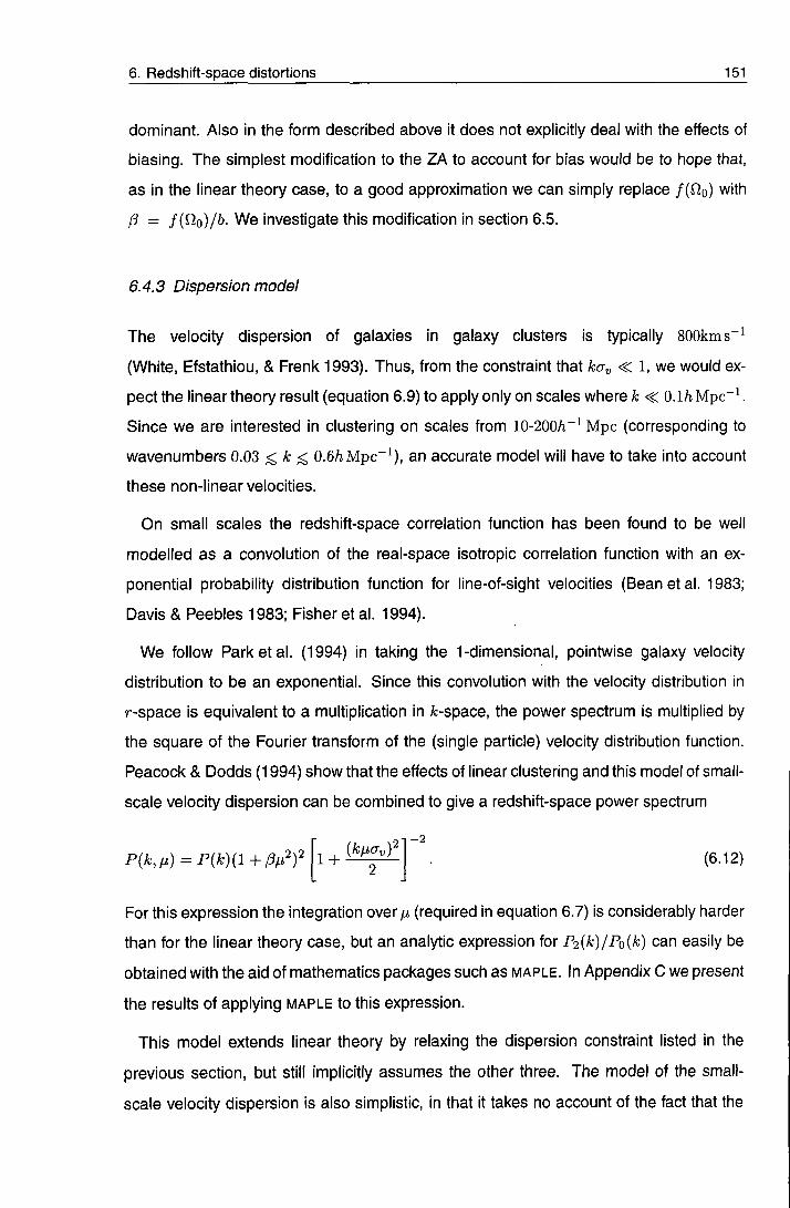
6. Redsh i f t -space distor t ions 151^
dominant. Also in the form described above it does not explicitly deal with the effects of biasing. The simplest modification to the ZA to account for bias would be to hope that, as in the linear theory case, to a good approximation we can simply replace / (OQ ) with 13 = / ( f2o ) /6 . We investigate this modification in section 6.5.
6.4.3 Dispersion model
The velocity dispersion of galaxies in galaxy clusters is typically 800km s"^
(White, Efstathiou, & Frenk 1993). Thus, from the constraint that Izoy « : 1, we would ex
pect the linear theory result (equation 6.9) to apply only on scales where < 0 .1 / iMpc~^
Since we are interested in clustering on scales from 10-200/i~^ Mpc (corresponding to
wavenumbers 0.03 ^ A: 0 .6 / iMpc~^) , an accurate model will have to take into account
these non-linear velocities.
On small scales the redshift-space correlation function has been found to be well
modelled as a convolution of the real-space isotropic correlation function with an ex
ponential probability distribution function for line-of-sight velocities (Beanetal. 1983;
Davis & Peebles 1983; Fisher et al. 1994).
We follow Parketa l . (1994) in taking the 1-dimensional, pointwise galaxy velocity
distribution to be an exponential. Since this convolution with the velocity distribution in
r-space is equivalent to a multiplication in A;-space, the power spectrum is multiplied by
the square of the Fourier transform of the (single particle) velocity distribution function.
Peacock & Dodds (1994) show that the effects of linear clustering and this model of small-
scale velocity dispersion can be combined to give a redshift-space power spectrum
2x2 P{k,tJ.)=P{k){l+Pfx') 2 - , - 2
(6.12)
For this expression the integration over |U (required in equation 6.7) is considerably harder
than for the linear theory case, but an analytic expression for P2{k)/Po{k) can easily be
obtained with the aid of mathematics packages such as MAPLE . In Appendix C we present
the results of applying MAPLE to this expression.
This model extends linear theory by relaxing the dispersion constraint listed in the
previous section, but still implicitly assumes the other three. The model of the small-
scale velocity dispersion is also simplistic, in that it takes no account of the fact that the
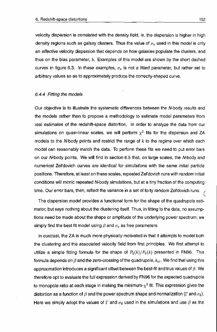
6. Redsh i f t -space distort ions 152
velocity dispersion is correlated with the density field, ie. the dispersion is higher in high density regions such as galaxy clusters. Thus the value of ay used in this model is only an effective velocity dispersion that depends on how galaxies populate the clusters, and thus on the bias parameter, b. Examples of this model are shown by the short dashed curves in figure 6.3. In these examples, ay is not a fitted parameter, but rather set to arbitrary values so as to approximately produce the correctly-shaped curve.
6.4.4 Fitting tfie models
Our objective is to illustrate the systematic differences between the N-body results and
the models rather than to propose a methodology to estimate model parameters from
real estimates of the redshift-space distortion. In order to analyze the data from our
simulations on quasi-linear scales, we will perform fits for the dispersion and ZA
models to the N-body points and restrict the range of k to the regime over which each
model can reasonably match the data. To perform these fits we need to put error bars
on our N-body points. We will find in section 6.5 that, on large scales, the N-body and
numerical Zel'dovich curves are identical for simulations with the same initial particle
positions. Therefore, at least on these scales, repeated Zel'dovich runs with random initial
conditions will mimic repeated N-body simulations, but at a tiny fraction of the computing
time. Our error bars, then, reflect the variance in a set of forty random Zel'dovich runs. ^
The dispersion model provides a functional form for the shape of the quadrupole esti
mator, but says nothing about the clustering itself. Thus, in fitting to the data, no assump
tions need be made about the shape or amplitude of the underlying power spectrum; we
simply find the best fit model using f3 and cr„ as free parameters.
In contrast, the ZA is much more physically motivated in that it attempts to model both
the clustering and the associated velocity field from first principles. We first attempt to
utilize a simple fitting formula for the shape of P2{k)/Po{k) presented in FN96. This
formula depends on /? and the zero-crossing of the quadrupole, kn\. We find that using this
approximation introduces a significant offset between the best-fit and true values of p. We
therefore opt to evaluate the full expression derived by FN96 for the expected quadrupole
to monopole ratio at each stage in making the minimum-x^ fit. This expression gives the
distortion as a function of /3 and the power spectrum shape and normalization ( r and as).
Here we simply adopt the values of r and as used in the simulations and use /? as the

6. Redsh i f t -space distort ions 153
single free parameter in the model. For real observations one could simultaneously fit for these parameters using estimates of the redshift-space power spectrum monopole,
Po{k).
6.5 Results
In figure 6.4 we compare the model predictions for the quadrupole ratio, P2{k)/Po{k),
with the results of the two unbiased N-body simulations. The points with error bars show
the N-body results. The model that produces the lower quadrupole ratios has Q,q = 0.3,
Ao = 0.7 and as = 1.13, and that with the stronger quadrupole signal has OQ = 1 and
as = 0.55. The error bars placed on the N-body results are indicative of the statistical
error we expect on an estimate of the quadrupole ratio, from a single realization, and are
obtained by taking the standard deviation of forty Monte Carlo realizations of the ZA. It
is clear that, apart from the first few points with k ^ 0 .07 /^Mpc"^ the deviation from the
constant ratio predicted by linear theory is large.
The solid lines in figure 6.4 are each for one ZA realization starting from the same
initial density field as the corresponding N-body simulation. This model reproduces the
N-body results extremely accurately at low-A;. For the Clo - 0.3 case the ZA and N-body
results match well up to A; 0 . 2 5 / i M p c " ^ which is beyond the scale at which P2{k)/Po(k)
becomes negative. This result is in complete agreement with the findings of FN96. The
only N-body results they studied were for a similarly normalized = 0.3,Ao = 0.7 model.
In the case of f2o = 1 we find much less impressive agreement between the ZA and
N-body simulations. The results begin to diverge at ;^ 0.15/iMpc~^ and differ very
significantly at = 0 . 4 2 5 / i M p c - \ where P2{k)/Po{k) = 0 for the N-body simulation.
Figure 6.5 shows another comparison between these N-body and ZA realizations. We
show the ratio of their estimated final power spectra to the expected linear power spectra,
ie. the initial power spectra evolved to ^ = 0 assuming linear theory We see that in the N-
body simulations the non-linear growth of structure leads to an increase in power on small
scales. This effect is strongest for fio === 0.3, which has the highest as and is therefore the
most non-linear. In contrast, the behaviour of the ZA simulations is the exact opposite;
shell crossing erases power on small scales. In this respect the agreement between ZA
and N-body is particularly poor for the OQ = 0.3 model. Even at mildly non-linear scales
the discrepancy is quite severe: evidently the accuracy of the ZA at modelling the ratio

6. Redsh i f t -space distor t ions 154
o
0.5
-0 .5 h
•1 h
ZA numerical I I I I I I 1 W-body
• Best fit CT, Best fit ZA
• 0 = 1 . 0
• 0 = 0.3
0.2 0.4 k / h M p c -
0.6 0.8
Figure 6.4: The quadrupole ratio P2{k)IPo{k) for two unbiased A/-body simulations compared with the
corresponding Zel'dovich approximation simulations and two model fits. The upper curves are for Qo = 1
and as = 0.55 and the lower curves for fio = 0.3, Ao = 0.7 and as = 1.13. The error bars on the W-body
results are indicative of the statistical error in our estimates and are estimated from the standard deviation
between forty ZA realizations. The solid lines show the results from single ZA realizations starting from the
same density fields as the W-body simulations. The long dashed and short dashed curves are model fits for
the ZA and dispersion model respectively. Only the first ten points have been used in constraining the ZA
fits, and the first thirty for constraining the dispersion model, as explained in section 6.5. The corresponding
best fit parameters and confidence intervals are shown in figure 6.7.
P2{k)/Po{k) Is either a coincidence, or this statistic is less sensitive to the shortcomings
of the method than the power spectrum itself is. Until this problem is investigated more
thoroughly we suggest that the success of the ZA should be treated with scepticism.
In our implementation of the ZA we have applied very little smoothing of the initial den
sity field. We have simply truncated the input power spectrum at the Nyquist frequency of
the particle grid used in the Monte Carlo realizations described in section 6.3.1 to facilitate
Inter-comparison. However, Melott, Pellman, & Shandarin (1994) have shown that, at
least for some statistics, the correspondence between the ZA and AZ-body simulations

6. Redsh i f t -space distor t ions 155
0^=1.0 N - b o d y n„=0.3 Af-body n„=1.0 ZA n„=0.3 ZA
0.2 0.4 k / h M p c - i
0.6 0.8
Figure 6.5: The ratio of estimates of the real-space evolved power spectra, P{k), to the linear theory
predictions, PLINEAR(A;), for the A/-body simulations and the corresponding ZA simulations. The models
are the same fio = 1 and f io = 0.3 models studied in figure 6.4.
can be improved by more severe smoothing of the initial density field. They define a
non-linear wavenumber, knu by
An / P{k)k^dk = Jo
(6.13)
and then smooth the initial density field with a Gaussian window, exp{-k'^/2k^), with
fcg = pkjii. They find that the best choice of the parameter p depends only weakly on the
shape of the power spectrum and is p ~ 1.25.
The consequences of adopting such a Truncated ZA power spectrum for our distortion
statistic are shown in figure 6.6. The introduction of additional smoothing worsens the
agreement between the N-body results and those of the ZA. In particular, for the degree
of smoothing advocated by Melott et al. (p = 1.25) the agreement between A/-body and
ZA is very poor. The smoothing applied is washing out the distortions we are trying to
measure. However, we find that in real space a mild amount of smoothing can produce
a power spectrum that is slightly closer to the N-body result, though this effect is rather
small.

6. Redsh i f t -space distor t ions 156
o (X \
CM
0.5
-0 .5
•1 h
ZA - Minimal smoothing Truncated ZA
I I I I I I I JV-body
0.2 0.4 k / hUpc-'
0.6
p = 1.00
= 1 .251
2 . 0 0 -
0.8
Figure 6.6: The dependence of the Zel'dovich approximation prediction for the ratio P2{k)/Po(k) on the
extent to which the initial density field is smoothed before applying the ZA. The error bars show the N-body
result for the flo = 1.0 model taken from figure 6.4. The dotted curve shows the ZA result for the minimal
amount of smoothing, ie, truncation at the Nyqulst frequency. The remaining curves show the effect of grad
ually increasing the smoothing using an additional Gaussian smoothing with ks = pk^i (see equation 6.13)
andp = 5.0,2.0,1.25 and 1.0.
The ZA and dispersion model fits are shown by the smooth long and short dashed
curves in figure 6.4. The corresponding best fit model parameters and confidence in
tervals are shown in figure 6.7 and table 6.2. Here the horizontal lines bracket the 68%
and 99.7% (1 - and 3-o-) confidence intervals of (3 for the ZA fit. The ellipses show the
corresponding confidence intervals for the two-parameter dispersion model. Both ZA
fits give a best-fit p that is within 1-a of the theoretical value, so there seems to be no
appreciable systematic error in our estimate. However, this result is achieved by limiting
the range of the fit to the first ten bins in A;-space, ie. k < 0 . 182 / lMpc - ^ in both models. At
smaller scales than this, particularly in the = 1 model, the fits can be seen to strongly
overestimate the redshift-space distortion. Thus if a fit were made to data covering a
wider range of scales, j3 would be severely underestimated. In contrast, the dispersion
model fits remain in reasonable agreement with the data up to much larger k. We fit
our data up to the thirtieth data bin, corresponding to a length scale of 11.5/i"^ Mpc. For

6. Redsh i f t -space distor t ions 157
0.8
<5a. • 0 = 1 . 0 , (3=1.0
0.6
0 .4
• 0 = 1 . 0 , 13 = 0.55 • 0 = 0 . 3 , (3 = 0A9
300 4 0 0 / k m s - i
500
Figure 6.7: The 68% and 99.7% confidence intervals (1- & 3-<T) of the model parameters for the fits shown
in figure 6.4 and figure 6.8. The ellipses are for the two-parameter dispersion model for the three different
simulations, and the horizontal lines for single-parameter ZA model for the two unbiased models for which
this provides a reasonably good fit. The best fit values of p and the per degree of freedom for the best fit
models are given in table 6.2.
0,0 = 0.3, the dispersion model analysis seems to be offset towards a low estimate of /?,
but this effect is fairly small given the size of the error contours. The fit itself is a very
good over the whole range of k in question. However, for fio = 1> /9 is systematically
underestimated by more than 10% at a high level of significance. This offset can be
understood by reference to the models shown in figure 6.3. In comparison to the ZA,
which is an accurate fit at low-fc, the dispersion model curve changes slope too rapidly
and is too shallow at low-fc, leading to an underestimation of p. We found this behaviour
to be the same for a variant of the dispersion model in which the small scale random
velocity Is assumed to be Gaussian rather than exponentially distributed. This alternative
Gaussian dispersion model produces a worse fit overall, and a more biased estimate of
p. The same effect is also expected to introduce an offset in the f^o = 0.3 simulation, but
it is rather smaller for this case and so is not easily detected.
As shown in table 6.2, we have calculated the one-dimensional rms peculiar velocity of
particles in each simulation, af^, in an attempt to look for a physical significance of the

6. Redsh i f t -space distor t ions 158
ay value found in the dispersion model fit. We do not expect this velocity to correspond to that obtained from the dispersion model fit, as this quantity should reflect the small-scale peculiar velocity, after velocities resulting from large-scale bulk flows have been subtracted. In order to compare like with like, we also calculate a small-scale dispersion, al^, in the following manner. A friends-of-friends algorithm is used to identify cluster membership for each galaxy and each cluster galaxy has its velocity in the simulation replaced with its relative velocity with respect to the parent cluster. Galaxies not tagged as being in a cluster are thrown out of the sample. Thus, af" should be closely related to the dispersion from the model fit. The results presented in table 6.2 clearly show that, in fact, this is not the case, and there is no simple relationship between the best fit dispersion and the true velocities of the galaxies over the range covered by our simulations.
/3 model /3fit F I T S I M ss
1.0 1.00 ZA 0.98 2.28
1.0 1.00 disp 0.87 2.03 306 365 300
0.3 0.49 ZA 0.48 0.86
0.3 0.49 disp 0.44 0.99 509 431 388
1.0 0.55 disp 0.56 1.39 379 425 331
Table 6.2. Best fit /? and goodness of fit (x^ per degree of freedom) indicator for our simulations under
the Zel'dovich and dispersion models. For the dispersion model we also show the best fit values of CT„
and compare with the one-dimensional velocity dispersion of the simulations, c r ^™, and the small-scale
dispersion, a^^, as explained in section 6.5. All velocities are measured in k m s ^ ^ Error contours for the fits
are shown in figure 6.7.
6.5.1 Biased models
In figure 6.8 we show the model predictions for the quadrupole ratio, P2{k)/PQ{k), for a
biased model with fio = 1 0 . The heavy curves show the results of selecting biased galaxy
catalogues by the three methods described in section 6.5.1. The differences between the
models at large scales are purely statistical, since different galaxies have been selected in
the different samples. At high k the two Lagrangian methods agree well, but the Eulerian
one systematically shows less distortion. This difference is to be expected as this method
populates evenly all regions with density higher than the threshold, rather than giving

6. Redsh i f t -space distor t ions 159
o
03
a,
ZA numerical ZA analytic N-body #1 W-body #2 W-body #3 Best fit a
0.4 k / hUpc-'
Figure 6.8: The quadrupole ratio, P2(/ i ; ) /Po(fc) , for biased fio = 1 galaxy catalogues with 6 = crl^^/crs = 1-81,
P = 0.55. The N-body lines show the results for our three different methods of constructing biased galaxy
catalogues from the A/-body simulation, as outlined in section 6.5.1. The thin solid line shows the result of
a ZA realization that has been biased in the same way as one of the N-body catalogues. The long dashed
curve shows the prediction of the ZA made by assuming as = ^ 1 * ' and f2o ® = 0 as proposed by FN96. The
short dashed line is a fit of the dispersion model to one of the N-body catalogues.
extra weight to the areas with higher density (and thus velocity dispersion), as the other
two models do.
The long dashed curve shows the prediction for the analytic ZA where, as suggested
by FN96, the model adopted assumes that galaxies are unbiased, as = crf', but with
f20-6 = 1/1.81 to match the value of /? = 1/6. This curve should be compared with
the results from a biased catalogue constructed from a realization of the ZA (thin solid
curve). Clearly these two curves do not agree, except at the very largest scales. We
cannot, then, use the simple linear theory modification to the ZA to account for bias if we
want to use data in any but the most linear regime. This result is perhaps to be expected
as bias will not only boost the galaxy density fluctuations with respect to the underlying
mass distribution, but will also preferentially place galaxies in dense structures where
random velocities produced by virialized structures are largest. The small scale velocity
field produced by shell crossing in the ZA is not a good model of the random velocities

6. Redshift-space distortions 160
produced in non-linear regions. For this reason the biased ZA realization is a poor fit to the N-body results. It diverges from the N-body result more rapidly than the corresponding model for the unbiased Oo = 1 simulation.
The short dashed curve is a fit of the dispersion model to the N-body peaks biased
galaxy catalogue. This model, with an exponential velocity distribution, determines /?
very accurately and is a good fit to the data over this range of scale. The fitted velocity
dispersion is ay = 380km s ~ \ 70km s"^ higher than the unbiased version of the same N-
body simulation, which illustrates how bias preferentially places galaxies in environments
with higher thermal velocities.
6.6 Discussion
We have used a set of high resolution N-body simulations to investigate the
accuracy of two models of the redshift-space distortion of galaxy clustering on
scales of 10-200/i~^ Mpc . We conclude that neither the Zel'dovich approximation
(Fisher & Nusser 1996; Taylor & Hamilton 1996) nor the linear theory plus random ve
locity dispersion model (Peacock & Dodds 1994) provides an accurate description of
redshift-space clustering. In general both models could lead to significant systematic
errors in the estimation of /3 = flo^/b when applied to the high precision data that will be
available from the large 2dF and SDSS galaxy redshift surveys.
The ZA provides a good fit in the unbiased cases on the very largest scales that we
have investigated. However, only for the low fio cosmology considered does this model
remain accurate over the full range of scales for which the quadrupole distortion is positive
{P2{k)/Po{k) > 0). In the case of biased galaxy catalogues, the ZA is a very poor
description of redshift clustering apart from on the very largest scales, where it tends
to the linear theory result.
Smoothing the initial density field prior to applying the ZA, as in the Truncated ZA, was
found to further worsen the agreement with the N-body results of redshift-space distor
tions. In general, then, we would only advocate using the ZA for analysis of unbiased
universes on scales down to ~ AOh~^ Mpc.
The two-parameter dispersion model was found to produce more acceptable fits to the
N-body results. However, only in the cases in which the small scale velocity dispersion
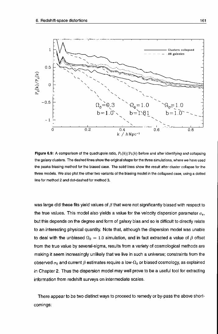
6. Redshift-space distortions 161
o CU
\
a,
0.5
- 0 . 5
•1 h
Clusters collapsed - 1
• . = 0.3 b=1.0"x
^=1.0 b="nai
-•o^=J.O b=1.0~
0.2 0.4 k / h M p c -
0.6 0.8
Figure 6.9: A comparison of the quadrupole ratio, P2{k)IPo{k) before and after identifying and collapsing
the galaxy clusters. The dashed lines show the original shape for the three simulations, where we have used
the peaks biasing method for the biased case. The solid lines show the result after cluster collapse for the
three models. We also plot the other two variants of the biasing model in the collapsed case, using a dotted
line for method 2 and dot-dashed for method 3.
was large did these fits yield values of /3 that were not significantly biased with respect to
the true values. This model also yields a value for the velocity dispersion parameter Oy,
but this depends on the degree and form of galaxy bias and so is difficult to directly relate
to an interesting physical quantity. Note that, although the dispersion model was unable
to deal with the unbiased 9,^ = 1.0 simulation, and in fact extracted a value of p offset
from the true value by several-sigma, results from a variety of cosmological methods are
making it seem increasingly unlikely that we live in such a universe; constraints from the
observed as and current p estimates require a low-fio or biased cosmology as explained
in Chapter 2. Thus the dispersion model may well prove to be a useful tool for extracting
information from redshift surveys on intermediate scales.
There appear to be two distinct ways to proceed to remedy or by-pass the above short
comings:

6. Redsh i f t -space distor t ions 162
• Improve the analytic models so as to produce accurate predictions over the full range of scales that will be probed by the redshift surveys.
• As our computers increase in memory and CPU power, the "brute force" approach of
simply running N-body simulations for the whole range of parameter space becomes
increasingly plausible. Here the dispersion model may be very useful in fitting and sug
gesting the approximate value of p, and thus putting restrictions on the combinations
of parameter values worth Investigating.
A promising approach following the first method is an extension of the model discussed
in Fisher (1995), where linear distortion effects on ^(CTJTT) are modelled as a convolu
tion with a Gaussian velocity distribution with scale- and orientation-dependent velocity
dispersion. Fisher suggests that this model may be adapted to deal with distortions in
the highly non-linear regime by replacing the Gaussian with a generalized distribution
function. This function should behave asymptotically as a Gaussian on large scales
but tending to an exponential with isotropic and constant velocity dispersion on small
scales. Hamilton et al. (1991) developed an accurate method of obtaining the non-linear
correlation function in real space, ^ ( r ) , using a universal scaling relation. This work
has been extended to the non-linear power spectrum for a range of initial power spectra
and cosmologies (Peacock & Dodds 1994; Jain, Mo, & White 1995). Mo, Jing, & Borner
(1996) outline a technique by which the quantities that define the velocity field (ie. mean
painwise peculiar velocity, vuir), painwise peculiar velocity dispersion, {vl2{r)), and mean
square peculiar velocity, (v'^)), can be modelled for a given cosmology and initial power
spectrum. Given reliable models for these quantities. Fisher's treatment should provide
a way of translating ^ ( r ) into the redshift-space statistic ^{a,iT), and thus calculating
precisely the anisotropy expected on any given scale. However, this method is still subject
to problems: namely finding out exactly how the velocity distribution function behaves on
intermediate scales, and developing a way for modelling the effects of galaxy bias.
If one is resorting to simulations then it may be possible to filter the data to remove
some non-linearities before commencing the analysis of redshift-space distortions. An
interesting procedure for doing this is to identify and collapse galaxy clusters. Since
their high velocity dispersion is responsible for much of the suppression of P2/P0, their
removal might lead to more robust estimates of p. Figure 6.9 illustrates the effect of
collapsing clusters in our simulations. As expected, the anisotropy is much closer to the

6. Redsh i f t -space distor t ions 163
linear theory prediction on large and intermediate scales. On small scales the quadrupole ratio converges on zero rather than becoming strongly negative. Cluster membership was established using a friends-of-friends algorithm, in which any pair of galaxies with separation less than 0.2 times the mean separation are classed as being in the same cluster. Each cluster member then has its velocity replaced with the mean velocity of the cluster itself, effectively eliminating the internal velocity dispersion of these virialized structures. The identification of galaxy clusters will be much more complex when dealing with real galaxy redshift surveys. Moore, Frenk, & White (1993) describe a way of applying this technique to the CfA survey using a redshift- and orientation-dependent linking length to define groups. Whatever algorithm one adopts can always be tested by running it on mock galaxy catalogues made from the N-body simulations.
Our assessment of the accuracy of these models is less positive than that of previous
investigations (FN96, Taylor & Hamilton 1996; Peacock & Dodds 1994) because:
• We do not "fix" the ZA. Earlier authors (FN96 and Taylor & Hamilton 1996) have
used the zero-crossing of the quadrupole-to-monopole ratio as an empirical parameter
derived from the data in order to scale the ZA curve. We feel this approach completely
denies the whole point of using the Zel'dovich approximation in the first place. Instead,
we calculate the full ZA because of its greater predictive power
• We use a range of simulations. Whereas previous work has generally used a single
cosmology to compare with the ZA or the dispersion model, we check the applicability
of the methods in a variety of cases, including a biased case, motivated by current ob
servations of the large-scale structure in the universe. We will apply similar techniques
to a much larger sample of cosmologies in Chapter 8.
• We demand mucli greater accuracy tlian previous worl<. Previous work has
generally focussed on applying redshift distortion models to existing samples, where
random errors are large. We, on the other hand, apply them to whole simulations with
well determined P(k ) . We feel this degree of rigour is justified, as future surveys will
give us data of comparable quality, and systematic errors that have previously been
deemed "small" will enter at a significant level.

6. Redsh i f t -space distort ions 164
Despite the failings of existing models pointed out in this work, redshift-space distortion analysis remains very interesting and promises to be of great use in extracting information from the next generation of galaxy surveys.
References
BallingerW. E., Peacocl<J. A., Heavens A. R, 1996, MNRAS, 282, 877
Bean A. J., Ellis R. S., Shanks T , Efstathiou G., Peterson B. A., 1983, MNRAS, 205, 605
Bouchet F. R., Colombi S., Hivon E., Juszkiewicz R., 1995, A&A, 296, 575
Bromley B. C , Warren M. S., Zurek W. H., 1997, ApJ, 475, 414
Cole S., Fisher K. B., Weinberg D. H., 1994, MNRAS, 267, 785
Cole S., Fisher K. B., Weinberg D. H., 1995, MNRAS, 275, 515
Colless M., 1995, The 2df galaxy redshift survey, http://msowww.anu.edu.au/'heron/Colless/colless.html
da Costa L. N., Vogeley M. S., Geller M. J., Huchra J. R, Park C , 1994, ApJ Lett, 437, LI
Davis M., Peebles R J. E., 1983, ApJ, 267, 465
Fisher K. B., 1995, ApJ, 448, 494
Fisher K. B., Davis M., Strauss M. A., Yahil A., Huchra J. R, 1994, MNRAS, 267, 927
Fisher K. B., Nusser A., 1996, MNRAS, 279, LI
Gregory S. A., Thompson L. A., 1978, ApJ, 222, 784
Gunn J. E., Weinberg D. H., 1995, in proceedings of the 35th Herstmonceux workshop Cambridge Univer
sity Press, Cambridge, astro-ph/9412080
Hamilton A. J. S., 1993, ApJ Letters, 406, 47
Hamilton A. J. S., 1997, astro-ph/9708102
Hamilton A. J. S., Kumar R, Lu E., Matthews A., 1991, ApJ Lett, 374, LI
Jackson J. C , 1972, MNRAS, 156, I P
Jain B., Mo H. J., White S. D. M., 1995, MNRAS, 276, L25
Kaiser N., 1987, MNRAS, 227, 1
Loveday J., Efstathiou G., Maddox S. J., Peterson B. A., 1996, ApJ, 468,1
Maddox S. J., Efstathiou G., Sutherland W. J., 1996, MNRAS, 283,1227
MatsubaraT, Suto Y., 1996, ApJ, 470,1
Melott A. L., Pellman T E., Shandarin S. R, 1994, MNRAS, 269, 626
Mo H. J., Jing Y R, Borner G., 1997, MNRAS, 286, 979
Moore B., Frenk C. S., White S. D. M., 1993, MNRAS, 261, 827
Park C , Vogeley M. S., Geller M. J., Huchra J. R, 1994, ApJ, 431, 569
Peacock J. A., Dodds S. J., 1994, MNRAS, 267,1020
Peebles R J. E., 1993, Principles of Physical Cosmology Princeton University Press, Princeton
Press W. H., Teukolsky S. A., Vetterling W. T , Flannery B. R, 1992, Numerical Recipes in FORTRAN, 2nd
edition. Cambridge University Press, Cambridge
Ratcliffe A., Shanks X , Parker Q. A., Fong R., 1998b, MNRAS, 293,197
Ratcliffe A., Shanks T , Parker Q. A., Fong R., 1998a, MNRAS, 296, 191

6. Redsh i f t -space distor t ions 165
Sargent W. W., Turner E. L., 1977, ApJ, 212, L3
Shectman S. A., Landy S. D., Oemler A., Tucker D. L., Lin H., Kirshner R. P., Schechter P. L., 1996, ApJ,
470, 172
Strauss M. A., Willick J. A., 1996, Physics Reports, 261 , 271
Tadros H., Efstathlou G., 1995, MNRAS, 276, 45
Taylor A. N., Hamilton A. J. S., 1996, MNRAS, 282, 767
Weinberg D. H., Cole S., 1992, MNRAS, 259, 652
White S. D. M., Efstathiou G., Frenk 0. S., 1993, MNRAS, 262,1023
Zel'dovich Y. B., 1970, A&A, 5, 84

Chapter 7
Statistical errors
THE ARGUMENT Future galaxy redshift surveys will enable us to measure the
redshift-space power spectrum of the galaxy distribution to a high degree of
accuracy In placing constraints on parameters derived from these results, it is
necessary to model the errors on the measured values of the power spectrum
as a function of wavenumber. We review methods of calculating these errors,
based on the assumption that the large-scale perturbations are well described
by a Gaussian random field. We show how this method can also be applied
to measurements of the quadrupole-to-monopole ratio used in determining the
redshift-space distortions of the surveys. We also outline a technique for accu
rately modelling the effect of the survey geometry itself on the measured power
spectrum, enabling us to remove the systematic biases thus introduced. Com
bining these techniques we estimate the accuracy with which various surveys
(2dF SDSS, PSCz) will be able to constrain the derived parameters as, r, and p,
representing respectively the normalization and shape of the power spectrum,
and the linear redshift-space distortion factor.
7.1 Introduction
With any parameter estimation in science, one compares a model with the data that have
been collected. In order to assess the statistical significance of a model fit, one must
have an estimate of the uncertainty present in each datum. For laboratory-based science
this can normally be achieved by making repeated measurements and assessing their
spread, thus obtaining a measure of the width of the distribution from which they are
taken. In astronomy this is rarely possible and we are left with two alternatives: Monte
Carlo simulation of the repeated measurements, for which it is normally necessary to
assume a certain combination of parameters for input into the simulations; or an analytic
7. Statistical errors 167
calculation of the error, which again will rest on certain assumptions about the data themselves. This latter method has been employed by Feldman, Kaiser, & Peacock (1994, hereafter FKP) , to est imate the variance In the measured power spectrum of density f luctuat ions f rom a galaxy redshift survey The key assumption they make is that all the long-wavelength modes have independent, Gaussian-distr ibuted Fourier components, in agreement with the available data on the Gaussianity of the large-scale density distribut ion.
In this chapter we concern ourselves with the accuracy with which we can measure
der ived parameters, such as the ampli tude of the power spectrum, from a galaxy survey
We first out l ine a method for assessing the effect of the survey geometry itself on the
power spect rum, which is crucial if we are to get the best use out of the data. We go on
to summar ize the results of FKP, who demonstrate how to derive an expression for the
var iance in the power spectrum, and then illustrate how this approach can be extended
to measurements of the quadrupole-to-monopole ratio of P ( k ) .
We finish by combin ing our knowledge of the systematic bias caused by the survey
w indow funct ion with the random errors found by a Monte Carlo technique to estimate
the conf idence limits on the derived parameter/S from a galaxy redshift survey We apply
this technique to the survey volumes of the PSCz, 2dF and SDSS catalogues to see how
accurately they will respectively be able to measure p.
7.2 Modelling the effect of the window function
Determinat ion of the galaxy density field from a redshift survey is affected by the finite
w indow of the survey itself. This is a familiar phenomenon throughout physics, occurring,
for example, in optics when a source is v iewed through a slit which imposes its own
diffraction pattern on the image, or indeed in branches of astronomy where measure
ments are made in the t ime domain , in which case the window function becomes the
length of t ime that the signal is recorded for.
The est imate of the power spectrum is similarly convolved with the shape of the survey
w indow funct ion. It is desirable to remove the effect of this convolution before using
the power spect rum to est imate physical parameters, or else the estimates themselves
are prone to systematic biases. One way of correcting the problem would be simply to

7. Statistical errors 168
perform a direct deconvolut ion with the window function, but this is prone to bias since the w indow funct ion, particularly the radial selection function, has to be estimated from the survey itself, and is hence not known with complete accuracy This problem can be overcome by using the iterative method of Lucy (1974). This is the approach used by Lin e t a l . (1996) for the Las Campanas redshift survey This method is successful on smal l scales, but on wavelengths of size comparable to the survey size, the shape of the est imated power spectrum can be seriously affected by the convolution and the iterative correct ion process becomes unstable.
We descr ibe below a technique for assessing this effect based on examining the results
of a w indow funct ion convolution on a model power spectrum that is close to that which
w e expect to observe f rom our current knowledge of large-scale structure. We thus obtain
a correct ion factor that can be appl ied to a measured P ( k ) to remove the effects of the
convolut ion.
7.2.1 The model power spectrum
In order to assess the effect of the window function on the power spectrum estimation,
we pick a mode l redshif t-space power spectrum based on physically realistic values of r,
as, (5 and (jy, the shape parameter, ampli tude, linear redshift-space distortion parameter,
and smal l-scale velocity dispersion respectively
We assume that the power spectrum can be model led with a r model transfer function
as given by Bardeen et a i . (1986), so the l inear power is
^ [ l + 3.89g + ( 1 6 . 1 9 ) 2 + (5.46g)3 + (6.71g)4]i/2-
Here q = k/T and we set n = 1, r = 0.25, as suggested by observations
of large-scale structure (Peacock & Dodds 1994). The normalization of Piik) is de
termined by the requirement that as, the variance in galaxy number density in
spheres of radius Sh~^ Mpc, be equal to 0.96, the value determined for APM galaxies
(Maddox, Efstathiou, & Suther land 1996). The relation between and the power spec
t rum is given by:
= ^ / W{K 8)'P{k)k'dk, (7.2)

7. Statistical errors 169
where
sinkR-kRcoskR
W{k, R) = 3 ^ p , (7.3)
is the Fourier t ransform of a spherical top hat function. We then take the line-of-sight
vector and for each k-mode define fj, to be the cosine of the angle between the line of
sight and the wave-vector. In order for this definition to make sense, we must make the
approximat ion that the entire galaxy sample being considered lies along a single line of
sight. Surveys have a finite angular extent, and we take the line of sight to be the average
direction of all the galaxies, ie. the direction of the centre of the redshift survey We use
the Kaiser formula (Kaiser 1987), derived in Appendix A,
X ( M ) = ( 1 + / 3 M ' ) ' (7.4)
to model the effect of l inear redshift-space distortions on the power spectrum. This
formula is only strictly valid in the small-angle approximation, ie. when measuring galaxy
pairs that are at smal l angular separation (Zaroubi & Hoffman 1996). We have thus
assumed that the distant observer approximation is valid over the whole survey and
that the who le survey has a single line of sight. This is generally not true of real surveys,
where , if they have a large opening angle, it is necessary to measure the redshift-space
power spect rum by decomposi t ion into spherical harmonics (Heavens & Taylor 1995).
This method is more complex than the simple three-dimensional Fourier transforms that
we employ, and we do not at tempt to model it here. A volume of the Universe subtending
a smal l opening angle has the same information content as the same volume placed
locally, and the goal of the harmonic decomposit ion method is to remove the effect of a
large opening angle on the clustering statistics in the local volume. We effectively do this
by placing the observer infinitely distant f rom the survey
W e model the effect of non-l inear velocity dispersions on the power spectrum by as
suming the velocit ies are drawn from a pairwise exponential distribution, thus multiplying
the power spect rum by a factor
E{k,n) = [l + {ka,i^f/2]-' (7.5)
In the fol lowing chapter it is shown that this form represents the analytic distribution that
is closest to that found in A/-body simulations for the redshift-space distortions.
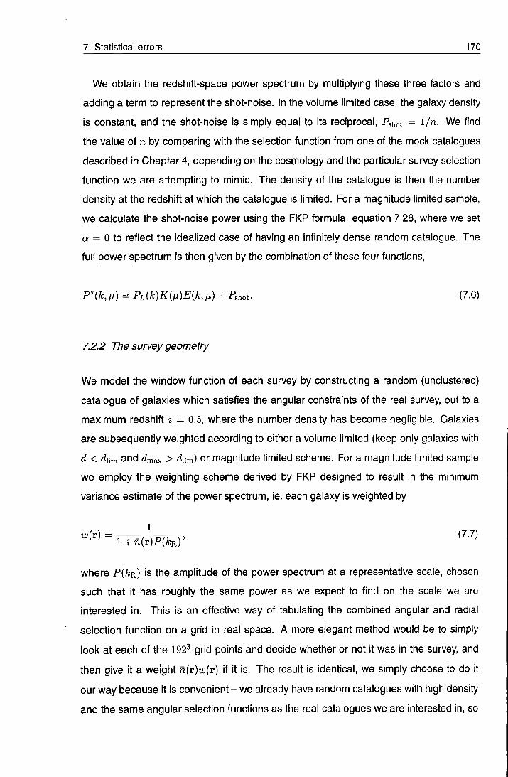
7. Statistical errors 170
We obtain the redshift-space power spectrum by multiplying these three factors and adding a term to represent the shot-noise. In the volume limited case, the galaxy density is constant, and the shot-noise is simply equal to its reciprocal, Pshot = We find the value of n by compar ing with the selection function from one of the mock catalogues descr ibed in Chapter 4 , depending on the cosmology and the particular survey selection funct ion we are at tempt ing to mimic. The density of the catalogue is then the number densi ty at the redshift at which the catalogue is l imited. For a magnitude limited sample, we calculate the shot-noise power using the FKP formula, equation 7.28, where we set a = 0 to reflect the idealized case of having an infinitely dense random catalogue. The full power spectrum is then given by the combinat ion of these four functions,
P%k,(,) = PLik)K{fi)E{k,fi) + Pshot. (7.6)
7.2.2 The survey geometry
We model the w indow function of each survey by constructing a random (unclustered)
cata logue of galaxies which satisfies the angular constraints of the real survey out to a
max imum redshift z = 0.5, where the number density has become negligible. Galaxies
are subsequent ly weighted according to either a volume limited (keep only galaxies with
d < c/iim and dmax > cJlim) or magni tude limited scheme. For a magnitude limited sample
w e employ the weight ing scheme derived by FKP designed to result in the minimum
var iance est imate of the power spectrum, ie. each galaxy is weighted by
where P ( A ; R ) is the ampl i tude of the power spectrum at a representative scale, chosen
such that it has roughly the same power as we expect to find on the scale we are
interested in. This is an effective way of tabulating the combined angular and radial
select ion funct ion on a grid in real space. A more elegant method would be to simply
look at each of the 192^ grid points and decide whether or not it was in the survey and
then give it a weight n ( r )u ; ( r ) if it is. The result is identical, we simply choose to do it
our way because it is convenient - we already have random catalogues with high density
and the same angular selection functions as the real catalogues we are interested in, so

7. Statistical errors 171
this crude method becomes attractive. Having constructed this window function, W{r), on the gr id, we Fourier transform it and normalize such that:
E l ^ ( k ) l ' = l - (7.8) k
This normal izat ion ensures that, when we convolve with the power spectrum, the total
power will be conserved. To assess the effect on the power spectrum we note that the
est imator of the power spectrum, P ( k ) , is given by
P ( k ) = \6{k)\'. (7.9)
The effect of mult iplying the density f ield, d{r), by the window function, i ;^ ( r ) , is described
in fc-space by the convolut ion:
6{k) = 6{k)(^W{k). (7.10)
Hence
P ( k ) - |^(k)(8>M^(k)|2. (7.11)
The convolut ion funct ion states that the convolution of two functions is equal to the
Fourier t ransform of the product of their Fourier transforms. Applying this law to the
inner convolut ion in the last equat ion gives
P ( k ) = \FT[Sir)W{r)]\\ (7.12)
and apply ing it in reverse to the outer product
F ( k ) = FT [[6{r)W{r)] ® [(5(r)W^(r)]] . (7.13)
The convolut ion can be writ ten
[S{r)W{r)] ® [Sir)W{r)] = {d{x)Wix)6{x + r)W{x + r ) ) , (7.14)
and , in the limit that the two fields 6{r) and W{r) are uncorrelated, this implies
P ( k ) = FT [{S{x)6{x + r ) ) ( W ^ ( x ) l ^ ( x -I- r ) ) ] , (7.15)

7. statistical errors 172
hence
P{k) = FT\^{r)[W{r)®Wir)]\ (7.16)
We square the fc-space window function and inverse Fourier transform it back into real
space, result ing in a funct ion that is the auto-correlation [W{r) 0 W{r)] of the survey
geometry. We inverse-Fourier transform the power spectrum and multiply the resultant
correlat ion funct ion by the survey auto-correlation before Fourier transforming back to get
the power spect rum estimator descr ibed by equation 7.16.
We thus obtain the convolved Po{k) and P2{k),
m ) = - y - P{k,,j.)Liifi)dfi, (7.17)
where Li is the Legendre polynomial of order /. The quadrupole statistic used for getting
P f rom redshift surveys fol lows f rom this expression.
7.2.3 Results
Figures 7.1 and 7.2 show the effect of the survey window functions on both the monopole
power, P{k), and the quadrupole-to-monopole ratio Q{k). As can be seen from these
plots, the effect of the window function can be highly significant. A survey with a broad
A;-space w indow funct ion causes significant smoothing of the power at large scales,
result ing in a ser ious mis judgement of the overall shape of the power spectrum. This is
part icularly signif icant when we are considering CDM-like models of the power spectrum
where r, the shape parameter, is a critical ingredient. The effect is again large for Q{k),
the convolut ion causing a serious damping of the quadrupole on large scales. Again,
it is this regime which is crucial to our understanding of large-scale structure, since the
information about the linear redshift-space distortion gives us a direct handle on the value
of Oo-
We conclude, then, that it is crucial to account for the window function convolution in
any measurement of the power spectrum or redshift-space distortion from galaxy redshift
surveys.

7. Statistical errors 173
4.4
4.2 CO
4
OX)
o ^ 3.8
" 1 — ^ — r 1—I—I—I—I—\—I—r 1 — r
N '•
/
^ 4
3.6
- / Inpu t
SDSS
2dF - SGP
PSCz
J I I 1 I I \ I I I I I I I I L
2 - 1 . 5 - 1 Logio[k (h Mpc- i ) ;
Figure 7.1: The effect of the window functions on the power spectrum for the three different surveys. We
use the volume limited case for the selction function as described in section 7.4.3.

7. Statistical errors 174
0.6
1—I—r 1—r n r
0.4
a-
0.2
0
/ / /
J I L
I n p u t
i -SDSS
i -
2dF - SGP\\\
PSCz
1 1 1 1 1 1 1 1 1 1
t.\"
\ 2 - 1 .5 - 1
Logio[k (h Mpc-O;
Figure 7.2: The effect of the window functions on the quadrupole-to-monopole ratio, Q, for the three different
surveys. This time we use the magnitude limited case with FKP minimum-variance weighting as described
in section 7.4.2.

7. Statistical errors 175
2
1.5
a.
0^
Of
0.8
0.6
0.4
0.2
0
1 I r
3 J I I I I I \ L
- 2 - 1
Log^Jk (h M p c - i ) ]
0
Figure 7.3: The model dependence of the convolution correction factor. The upper panel shows the correc
tion to the monopole power, the lower one to the quadrupole-to-monopole ratio, for five models: a standard
one with (r,/?,a^) = (0.25,0.55,650kms~^) (solid line), and variants; p = 1.0 (dotted line), r = 0.15 (short
dashed line), (T„ = 4 0 0 k m ( l o n g dashed line), and T = 0.5 (dot-dashed line).

7. Statistical errors 176
7.2.4 Model dependency
Using this technique to correct for the effect of the survey convolution is model dependent,
in that we have assumed parameters for the power spectrum used in making the correc
t ion. There are three parameters that are chosen, r, a^, and /?. A model dependency
introduces a possible loss of generality in the treatment, and a potential systematic bias
in the est imat ion of these parameters from the data. In figure 7.3 we examine the extent
of this model dependency in the monopole power spectrum, PQ, and the quadrupole-
to-monopole ratio, Q. In each case we plot the ratio of the convolved statistic to its
"true" value, ie. the analyt ic result coming from the correct choice of the power spectrum
parameters.
For the monopole power in the upper panel, it can be seen that the different models
can have a dramat ic effect on the correction function at large scales. The chief cause of
d iscrepancy is wi th the models with different r-values. The convolution effectively wipes
out information on the large-scale shape of the power spectrum. The convolved power
spect rum is insensit ive to r, and hence the required correction changes substantially
Other considerat ions have little effect, with a slight change in the large-scale power for a
substant ial change in /?. Unsurpr is ingly changing ay has no effect at large scales on the
power spect rum.
The variat ion of correction function with r is potentially problematic. To overcome it, we
could correct the power spectrum with a variety of r values and find the one with the best
goodness-of-f i t , or f ind an analytic description for the variation of the correction factor
with this parameters, and build it into the fitting procedure. Either way the degeneracy
increases the uncertainty on r. In section 7.4.4 we will assess the magnitude of the
systematic bias and compare it with the random error on this quantity.
Note that values of as will probably be unaffected by the wrong choice of correction
funct ion. The ampl i tude of f luctuations in spheres of radius 8/i~^ Mpc is dominated by
contr ibut ions f rom modes with wavelengths ~ 30/i~^ Mpc. Examining figure 7.3, it will
be seen that the Po curves have all converged by A; w lO'^-^hUpc-^, ie. wavelength
100/i~^ Mpc . So the variation in as will be small .
The quadrupole- to-monopole ratio generally seems more robust than PQ. The different
curves deviate near the zero crossing, but this is a numerical effect due to dividing by very

7. Statistical errors 177
smal l numbers. However, there is a systematic tendency for the value of the convolved
funct ion to be smal ler than its true value. This is easily explained. The convolution means
that close bins are correlated. Thus, a measurement of Q at a particular wavenumber is
really a weighted average over nearby modes. Since the gradient of Q increases with k,
this average will general ly be biased low compared to the real value at that scale. Thus
Q will be lower than Qtrue. and go through zero earlier, which is why all the curves in the
lower panel of f igure 7.3 turn down to the singularity. This could also be the cause of the
sl ight upturn in the upper panel of this f igure; non-linear effects cause the slope of Po to
become shal lower with k, and hence the bias is in the opposite direction.
We will assess the magni tude of the systematic bias introduced in (3 in section 7.6.2.
For now, we note that Q behaves approximately linearly to changes in /3. The scatter
between the different curves is, at most, of order 5%. Hence, adopting the wrong
correct ion factor can only bias /3 by ~ 5%. We shall later show that this is liable to be
rather smal ler than the random uncertaint ies.
7.3 The error on the power spectrum
The principle behind the analytic calculation of the variance is the assumption that each
Fourier mode of the galaxy distribution is an independent Gaussian random variable
drawn f rom a distribution with ampl i tude given by the power spectrum at this value of
k. The assumpt ion of Gaussianity is one that falls in with the theoretical prejudices of
the Standard model . If the density perturbations we see today on large scales were
seeded by quantum fluctuations in the early Universe, their distribution should indeed
be Gauss ian. On the other hand, if some non-standard physics is responsible for struc
ture format ion, such as the decay of textures, strings, or monopoles, the distribution is
expected to have non-Gaussian qualit ies. Probing primordial Gaussianity is a difficult
exper imental task, as departures from it are generally expected to be small, and will
only show up at long-wavelengths. On smaller scales, non-linear evolution is expected
to produce a non-Gaussian signature regardless of the initial condit ions. A variety of
techniques have been used, including topological studies of the present-day galaxy dis
tr ibution (Canavezes et al . 1998; FKP) and examination of the cosmic microwave back
ground using COBE data ( K o g u t e t a l . 1996; Ferreira, Maguei jo, & Gorski 1998). The
genus statistic approach has general ly found that Gaussianity cannot be ruled out with

c
7. Statistical errors 178
the use of current data sets. FKP themselves describe a method of using their power
spect rum analysis as a test for non-Gaussianity. If the power is Gaussian distributed, the
cumulat ive distribution of power est imated for each mode is exponential (Stuart 1987).
This relation is used to show that the power spectrum of the IRAS QDOT survey
(Rowan-Robinson et al . 1990) obeys the Gaussian hypothesis to a very high degree.
However, it has subsequent ly been shown (Fan & Bardeen 1994) that such one-point
statistics do not truly probe the Gaussianity of the underlying field, since a non-Gaussian
f ield can still have Gaussian distributed Fourier components. Ferreira, Magueijo, & Gorski
(1998) claim to have found evidence in the four year COBE data that rules out the
Gauss ian hypothesis at the 95% confidence level, using a new statistic that is highly
sensit ive to non-Gaussian f luctuations.
There is, then, some controversy over the nature of primordial f luctuations, but we note
for this work that departures from Gaussianity are small if they do indeed exist, and the
fol lowing t reatment is thus likely to be approximately valid.
We commence by calculating the scatter on the measurement of the amplitude of a
single wavelength mode. We then describe different techniques for combining these
errors to get a measure of the total uncertainty in the spherically averaged P(A;).
7.3.1 Variance from one mode
Consider ing the power in a field of real and imaginary components, Sr and 6i, the
est imator of the power spectrum, P{k), is given by
P{k) = Sl + 6j (7.18)
The power spect rum itself is def ined as
P{k) = (P{k)) = 2(4) = 2{6j) = {6l + 5]) (7.19)
Def ining 5P{k) as P(A;) - P{k), the variance in the estimate of the power in this mode is
given by = {6P{k)6P{k)). Expanding this we obtain
a' = {{sl + 6j-P{k)) [sl + 6]-P{k)))
= p{k? - 2P{k) {sl + s j ) + ( ( 4 + sj) {si + s j ) )
= {{Slf + 2{SlSj) + iSj)') - P{kf (7.20)

7. Statistical errors 179
We now apply the general relation for a bivariate Gaussian in x and y,
(xV) = {x^){y^)+Hxy)^{x^){y^)-{xyf (7.21)
Consider ing the two cases where x and y are either completely correlated (ie. identical)
or completely uncorrelated,
f 3(2;^)^ for X and y equivalent { x V ) = \ • (7.22)
I (a;^)(?/^) for X and y completely uncorrelated
Thus ,
= {Z + 2xl+Z){5lf -P{kf
= P{kf. (7.23)
So, single measurements of the power in one A;-mode will generally be distributed with
a scatter equal to the mean power at this wavelength. The analytic derivation of the
var iance proceeds by assuming that, to get an estimate of the one-dimensional quantity
P{k), we spherical ly average the three-dimensional P ( k ) into shells with |k| « k.
7.3.2 FKP1: simple mode-counting errors
If we have N independent measurements of the power for modes within the spherical
shell |k| K. k, the error on the mean goes down as -/N. In the notation of FKP,
P{k) = y j d'k'P{k'), (7.24)
where Vk is the vo lume (in A;-space) of the shell being averaged over. The variance is
given by
- {[P{k) - P{k)f) ^ ^ J d ' k J d'k'{6P{k)6Pik')). (7.25)
The key result of FKP is their equat ion 2.2.6,
{dP{k)SP{k')) = |P (k )VF(k - k ') + 5 ( k - k ' ) | ^ (7.26)
where
^ / d 3 r n ^ ( r ) ^ ^ ( r ) e ^ - -^ W - ;d3rn2( r )? i ;2 ( r ) ' ^ '
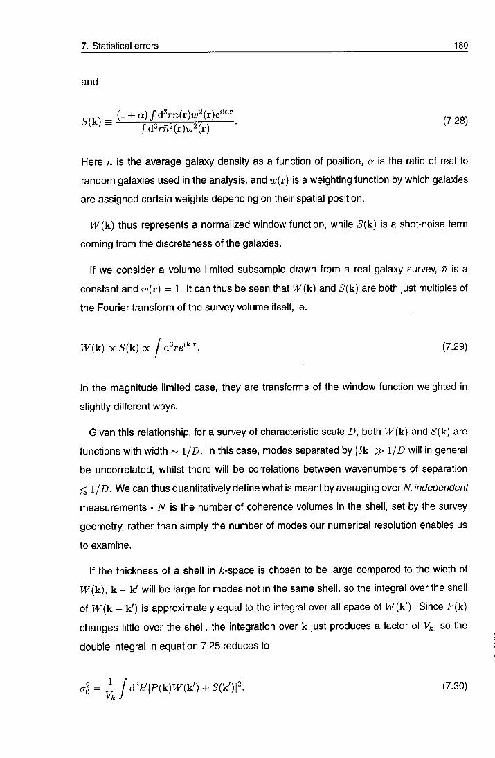
7. Statistical errors 180
and
J d'*rn^(r)t( ;^(r)
Here n is the average galaxy density as a function of posit ion, a is the ratio of real to
random galaxies used in the analysis, and u;(r) is a weighting function by which galaxies
are ass igned certain weights depending on their spatial posit ion.
W{k) thus represents a normal ized window function, while 5 ( k ) is a shot-noise term
coming f rom the discreteness of the galaxies.
If w e consider a volume limited subsample drawn from a real galaxy survey n is a
constant and u;(r) = 1. It can thus be seen that W{k) and S'(k) are both just multiples of
the Fourier t ransform of the survey volume itself, ie.
W(k) oc 5 ( k ) oc J dVe^•'•^ (7.29)
In the magni tude l imited case, they are transforms of the window function weighted in
slightly different ways.
Given this relationship, for a survey of characteristic scale D, both W{k) and ^ ( k ) are
funct ions with width ~ 1/D. In this case, modes separated by \6k\ > l/D will in general
be uncorrelated, whilst there will be correlations between wavenumbers of separation
^ 1 /D. We can thus quantitatively define what is meant by averaging over TV. independent
measurements - N is the number of coherence volumes in the shell, set by the survey
geomet ry rather than simply the number of modes our numerical resolution enables us
to examine.
If the thickness of a shell in A;-space is chosen to be large compared to the width of
W{k), k - k ' will be large for modes not in the same shell, so the integral over the shell
of W{k - k') is approximately equal to the integral over all space of W{k'). Since P ( k )
changes little over the shel l , the integration over k just produces a factor of 14, so the
double integral in equat ion 7.25 reduces to
^o = ^J d^A; ' |P(k)T^(k ' ) + 5(k')p. (7.30)

7. Statistical errors 181
Subst i tut ing for W{k) and 5 ( k ) , and Fourier transforming, leads to an expression for the fractional var iance in the power spectrum,
aj i2nrfdhn'w'[l + {l + a)/nP{k)]^ P2 Vk [/d3rn2t/;2]2 • ^^-^ '^
So, for any given form of n ( r ) and w{r) we can calculate a quadratic form for the de
pendence of the fractional error on wavenumber. Assuming an extremely dense random
catalogue such that a 0,
a2 _ (27r)3
where
^ , ^1 . ^2 P{k) P{kr\'
(7.32)
[ /d3rn2u;2]2- (7-33)
Aga in , we illustrate with the simpler expression for a volume limited subsample where
we can take n and w out of the integrals,
al _ {2nr [l + il + a)/nPik)]' P2 Vk Jd^r • ^^•''^^
As a consistency check, consider the power spectrum of a full, periodic simulation cube -
in this case, W{k) and 5 ( k ) , being discrete Fourier transforms of the whole volume, are
only non-zero for the A; = 0 mode, and so are proport ional to Kronecker 5-functions, 6K-
Meanwhi le ,
/ d^r = Volume of cube = X l o x i (7.35)
and the vo lume of a spherical shell in k-space is the number of modes in that shell times
the vo lume of one A;-mode,
Vk = NkiAkf = Nki^f. (7.36)
Thus , under the assumpt ion that we ignore discreteness effects (ie. no Poisson shot-noise
term),
_ (27r)3 J _ _ J _ P2 - Vk / d 3 r iVfc' ^ ^
so the error goes as l/y/Nk, exactly as expected. Away from this idealized case, the
method predicts that the fractional variance is the square root of the number of coherence
vo lumes in a A;-space shell .

7. Statistical errors 182
7.3.3 FKP2: more complex method
FKP note that the above expression will blow up when the shell width is thin compared
to the coherence length. They introduce the full expression for the uncertainty, which is
better behaved and tends to a constant value as the shell size decreases:
^0 = 4 E E \Pimi^' - k " ) + S{k' - k")\' (7.38) ^"k k' k"
(FKP equat ion 2.4.6). Apply ing the same consistency check as used above, we ignore
the shot-noise term and set W{k) = 5 K ( k ) . Performing the inner summation over k", we
thus obtain
-o = 4El^ (k )P- (7-39) k'
Now, there are by definit ion iV^ modes in the shell we are averaging over; hence, per
forming the remaining summat ion leads to
4 = — • (7.40) Pi Nk
This is twice the error that would be expected from equation 7.37. This apparent incon
sistency is easily resolved. When calculating the power spectrum we have taken the
complex Fourier transform of the density field, 6{r), which has no imaginary component.
Th is implies that S{k) is hermit ian, and hence P ( k ) = P ( - k ) . Thus, if we sum over a//the
modes in a spherical shell in A;-space, we would count Nk modes, where Nk is actually
twice the number of independent modes. This is the source of the discrepant factor of
two between equat ions 7.40 and 7.37. In practice, then, we save computation time by
only summing over the Nj independent modes in one hemisphere in fc-space, leading to
= 1^ E E l ^ ( k ) W ( k ' - k " ) + S{k' - k")p. (7.41) k' k"
7.3.4 Monte Carlo method
The double summat ion method (FKP2) is very CPU intensive If one has to sum over every
mode in the same shell , especial ly at high k where there are many modes in each shell.
We must therefore look to alternative, faster methods for power spectrum estimation.

7. Stat ist ical errors 183
It was ment ioned in section 7.3.3 that to obtain the full covariance matrix, we would need to run a large set of /V-body simulations, each with a random set of initial density waves, but the same cosmological parameters. We would then extract mocl< catalogues f rom each simulat ion and measure their power spectra to compare the cross correlation between k-modes. This technique would accurately measure the variance on all scales, but would be enormously t ime consuming for large surveys like 2dF and SDSS since each simulat ion takes many CPU hours to run, and we need a large number of simulations to est imate the variance reasonably well . In Chapter 8 we will present the results of apply ing this method crudely, using the variance between ten realizations for a particular cosmological model .
In this sect ion, we utilize the method of assessing the window function described in
sect ion 7.2. We assume that each individual k-mode of the density field is given by the
square root of this power spectrum multiplied by a complex number containing a pair
of Gauss ian random variables as the real and imaginary parts, thus satisfying equa
t ions 7.18 and 7.19. We Fourier transform the resultant S{k), and set the imaginary part
to zero, giving an overdensity f ield, 6{r). We note that setting the imaginary part to zero
effectively w ipes out half the power, so we multiply the resultant field by a factor of ^/2
to compensate for this. Then , as in the real case, we multiply by the window function
of the survey, thus introducing the necessary convolution. We then perform a power
spect rum analysis on the resultant mock survey and estimate the variance on the power
by repeat ing the procedure fifty t imes.
Figure 7.4 compares the three different methods outl ined here. It can be seen that the
Monte Carlo method is well approximated by the simple FKP1 error, which, at low-fc, is
close to the FKP2 curve. We do not model the shot-noise contribution from the FKP2,
as this causes the computat ion to be even more t ime-consuming, but this comparison
demonstrates that the methods are equivalent.
7.4 Error on derived parameters
We are now in possession of an accurate model for both the effect of the survey geometry
on the power spectrum and the value of the uncertainty in the power spectrum as a

7. Stat ist ical errors 184
0
-0.5
a. 1 -
T I I r
^ - 1 . 5
- 2 . 5
FKPl
FKP2
MC
I I I L J I I L J I I L
- 1 .5 -1 -0 .5 Log^Jk (h Mpc-i);
0
Figure 7.4: The fractional error on the monopole power spectrum, Po (A;), under the three different estimation
schemes. The solid line shows the simple FKP1 error, the dotted line the FKP2 (double summation method),
and the dashed line is the error derived from Monte Carlo realizations of the overdensity field.

7. Stat ist ical errors 185
funct ion of scale. In order to derive model parameters from the power spectrum, we will measure the ^ statistic for a model fit to the data,
) / p . _ p m o d / - ^ . \ ^
= E ' (7.42) T V /
where d is the correction to the power spectrum caused by convolution with the window
funct ion, and P'^°'* is the model power spectrum.
The parameters est imated directly from the power spectrum are r and CTS; we shall
assume that we are in possession of the real-space power spectrum and hence that ^
and cr„ are irrelevant. Alternatively, we are measuring the shape and amplitude of the
redshif t-space power spectrum. Under this assumption we are able to rapidly find the
values of the model parameters for which the fit has the minimum x^. From the values of
around this min imum, we can construct an error ellipse for the 1,2 and Za likelihood
regions in parameter space, using table 7.1 to f ind the A x ^ corresponding to the 68.3,95.4
and 9 9 . 7 3 % conf idence intervals for a fit with two degrees of f reedom. We can also predict
1,2 and 3 a errors on r and individually by taking the same confidence intervals for a
fit with one degree of f reedom, ie. A x ^ = 1,4 and 9, and f inding the projection of these
el l ipses onto the r or axes, as shown in figure 7.5.
Table 7.1. Values of A x ^ for l-,2- and 3-a results for different numbers of degrees of freedom, v.
Signif icance Probability A x ^
V = 1 z/ = 2 i/ = 3
l a 68.3% 1.00 2.30 3.53
2 a 95 .4% 4.00 6.17 8.02
3 a 99.73% 9.00 11.8 14.2
We are left wi th the choice of what A;-scale to extend our fit to. We note that our simple
model for the power spectrum should not be expected to be accurate very far away from
the l inear regime. Hence we define a non-linear scale, fcni, equal to the wavenumber at
wh ich the quadrupole estimator crosses through zero. We restrict all our fits to fc < fcni.

7. Statistical errors 186
1 \
A x ^ = 1 A x ^ = 1
Figure 7.5: Error on /3 from our two parameter fit. The dashed contour, Ax^ = 2.30 contains 68.3% of
normally distributed data, but the \a error on /? is obtained by projecting the extremities of the Ax^ = 1 error
ellipse on to the /3 axis.
We measure the power spectrum from one of the simulations presented in Chapter 4.
The cosmology we select is f i o = 1 with power spectrum normalization chosen to match
the observed abundance of rich clusters. For this simulation, we find a zero-crossing in
the quadrupole at k^\ = 0 . 2 5 / i M p c ~ ^ This prompts us to use a model power spectrum
with ay = 6 5 0 k m to obtain the same zero-crossing.
We note that, for thin shells, the double sum method and the Monte Carlo method of
error est imat ion tend to produce constant values of ao{k)/Po{k), independent of the shell
thickness. Thus , if we double the size of the grid used in the FFT analysis of the power
spect rum, each shell in A;-space has the same variance as it did before, but we are now
measur ing the power at twice as many values of k. Thus, when applying a statistic to
the data, a certain change in model parameter values would now produce twice the value
of Ax^ as before. So, we would conclude that the error on the derived parameter has
decreased - but it is obviously unreasonable that the accuracy should depend this much
on the size of the grid used. The problem arises because we are effectively over-using the
data; using thinner shells simply introduces correlations between the shells themselves,
but the total information content of the data remains the same. This problem is resolved
if the full covar iance matrix is used in a maximum likelihood method, as FKP do for the

7. Stat ist ical errors 187
Q D O T sample, rather than using the simple x^ technique which is equivalent to maximum likel ihood in the regime where the data are uncorrelated.
This method is t ime consuming, and, though we will employ it in the rest of this chapter,
we can get a good est imate of the error using the simple F K P l method. We showed in
sect ion 7.3.2 that this method is equivalent to the more complex one when the volume of a
k-mode used in the analysis is equal to the coherence volume of the survey: equivalently
when the vo lume of the grid is equal to the volume of the survey. At this point, the
survey is entirely descr ibed by the Fourier modes present on the grid, and modes are
uncorrelated. Moving to a larger grid size, we again increase the number of data points
in the x^ analysis, but the volume of each spherical A;-space shell, and hence the number
of coherence vo lumes contained within it, has decreased, increasing the individual errors
in such a way that the value of x^ is kept constant. Since it is desirable that the error
on der ived parameters should be independent of the grid size used for the analysis,
the F K P l method accurately predicts the error on quantit ies derived from the power
spect rum.
7.4.1 The full covariance matrix
Under the assumpt ions of F K P l , the ability of a survey to measure derived parameters
is entirely dictated by its volume. Whilst this is true to first order, in fact survey geometry
can play an important role as wel l . A non-uniform survey can contain information about
modes longer than those represented in a box of equivalent volume, since it has pairs of
galaxies at larger separat ion than the box length. Such a survey is, therefore, not fully
character ized by this collection of wavelengths. The equivalent volume assumption will
thus lead to an over-predict ion of the error; this is especially true if we are looking at
parameters that are mostly determined by the linear end of the power spectrum, since
a few extra modes at these scales can be worth many modes at smaller scales where
they are of less consequence. In order to fully assess this effect, we employ the full
covar iance matrix of the data points, derived from the Monte Carlo method used to obtain
the var iances. The goodness of fit is now given by the full expression for x^>
x ' = A.M.A^ (7.43)

7. Stat ist ical errors 188
where A is the vector of differences between model and data, and M is the inverse of the covar iance matrix. In the case of no correlations, this reduces to the simple x^ formula (equat ion 7.42). In this case, it can be seen that M reduces to a diagonal matrix whose e lements are given by Ma = 1/af. In the case of correlations between the data-points, much of the information contained in the matrix is redundant. We can thus restrict our analysis to the principal components, linear combinations of the data that contain nearly all the information. The matrix is fully describe by its n modes. However, we can choose to descr ibe the matrix using a fewer ( m < n ) principal components by discarding those that contr ibute little to the overall variance. We obtain the principal components using singular value decomposi t ion of the covariance matrix. Singular value decomposit ion of the matrix S returns the matrix U, where
S = U.W.U'^. (7.44)
W is the diagonal matrix containing the singular values. Where most of the n values of
W are very smal l , the input matrix can be well approximated by the first few principal
components . The inverse, M = can be approximated by
S-^ ^Ur.W-\U^, (7.45)
where the r denotes the reduced matrix, ie. that having only the first m columns. We
choose to keep the first m modes such that they contribute to 9 9 % of the total variance,
ie.
m n J2Wii = 0.99x^Wii. (7.46)
1 1
The effect of apply ing this selection criterion to the principal components can be quite
dramatic; for example, the analysis of the the 2dF SGP on a 2 0 0 4 ^ - ^ M p c grid results in
the select ion of only m = 39 components out of a total n = 8 1 , implying that only half the
modes make a substantial contribution to the variance.
Wavenumbers that measure the power spectrum on scales where its amplitude is
smal l will have correspondingly small absolute variances. In order to avoid discrimination
against these modes we first normalize the covariance matrix by Oij -> aij/^auajj.
As an il lustration of this method, we show in figure 7.6 a surface plot of an example
covar iance matrix. This matrix has been obtained using fifty random realizations of the

7. Stat ist ical errors 189
Figure 7.6: Surface plot of the covariance matrix. The matrix has been normalized so the on-diagonal
elements have unit height. A; = it' = 0 is in the upper left corner It can clearly be seen that the convolution
with the survey window function has the effect of smoothing the central peaks and introducing covariance
between A; / fc' modes, with width \k - k'\ ^ 1/D, where D is the width if the survey window function in
r-space.
overdensity and is normal ized as descr ibed above. The matrix is close to diagonal, with
the small f luctuat ions off to the sides being caused by the finite number of realizations,
but it can clearly be seen that the window function causes a smoothing of the central peak
into the nearest three or four off-diagonal modes. The smoothing scale is independent of
the value of k, so adjacent modes are similarly correlated at all scales.
We now apply this technique to calculate the uncertainty on r and ag when measured
using the w indow funct ions used in creating the mock catalogues described in Chapter 4 .
The technique is appl ied to the already completed PSCz survey of IRAS galaxies,
the 2dF South Galactic strip, and the Sloan Digital Sky Survey. We do this for the full
magni tude l imited catalogues and for volume limited subsamples.

7. Stat ist ical errors 190
7 .4 .2 Magnitude limited case
The use of the full magni tude limited catalogue is obviously desirable since we keep
the max imum amount of information. FKP derive a minimum variance weighting for the
galaxies in a magni tude l imited sample that provides the opt imum measure of the power
spect rum for a given value of P{k). The weight ing scheme effectively down-weights
galaxies near the observer, where the expected number density is high and the error is
dominated by the finite number of f luctuation volumes, and gives more weight to galaxies
at large distances, where shot noise dominates the error.
Our only choice in this case is the value of P ( A ; R ) used in the weighting scheme. In
general , we are most interested in the linear end of the power spectrum, and it would be
useful to have error-bars as small as possible in this regime; hence we choose a value of
P{kR) = bOOOh"^ M p c ^ . This is close to the value on large scales, and we note from FKP
that the error analysis is relatively insensitive to small changes in P{kR).
PSCz 2 d F - S G P SDSS
r 15.8% 4.7% 2.1%
as 14.4% 5.9% 2.5%
Table 7.2. l-a percentage errors on r and ag. The results are for the magnitude limited case, using the full
catalogue with FKP minimum variance weighting (P(A;R) = bOOOh'^ Mpc^), as described in section 7 .4 .2 .
In table 7.2 we show the results of applying this method to the survey volumes of the
PSCz, 2dF and SDSS catalogues. We find that, in general, the errors on the parameters
der ived f rom the power spectrum are rather low - current best estimates of the value of
r happi ly range between 0.2 and 0.25, for instance, implying that our current ;^ 10% level
of uncertainty will be radically improved upon in the next decade.
Several caveats, however, must be made in applying these results to the real surveys.
Firstly, a galaxy redshift survey is performed in redshift, rather than real space, and
the monopole power spectrum is distorted by the peculiar velocities of the galaxies we
observe. A l though we model a redshift-space power spectrum, our analysis of the errors
on r and as assumes that the data can be perfectly corrected for the redshift-space
distort ions. In the rest of this chapter, we will demonstrate a technique for deriving the

7. Stat ist ical errors 191
error on /3, the redshift-space distortion parameter, and we will f ind that it is generally much less wel l -determined than the errors given above. On linear scales, the redshift-space distort ions provide a constant boost to the power spectrum, and since it is these scales that determine r, the value of the shape parameter will not be much affected by this effect. The ampl i tude, as, is, however, severely degenerate with this boost, since the observed power spectrum depends on the product of the amplitude with the linear boost factor,
Pik) <xal(^l + f + ^ j (7.47)
(Kaiser 1987). We can calculate the degeneracy of p and as by taking differentials at
constant P{k), leading to the expression that
Aas / A ^ _ m + PV5 as / 0 1 - f 2/3/3 +/32/5 • ^'-^"^
This factor varies between 0.16 for p = 0.5 and 0.29 for /? = 1.0, so the fractional error
on as der ived f rom the redshift-space power spectrum can never be less than roughly a
sixth of the fractional error on p.
We also point out that the simple, two parameter power spectrum is a gross oversim
plif ication of the true power measured from a redshift survey, even once the correction
has been made accurately into real space. In reality, non-l inear clustering occurs at quite
moderate wavenumbers , and one is forced to either use a model with more parameters or
to restrict the search for information about the linear power spectrum to higher wavelength
modes. Given the behaviour of the errors with wavenumber, the fits are generally domi
nated by the low variance, quasi- l inear part of the power spectrum. In the real Universe,
this regime can be far less sensitive to r than in our simple model , thus it is important to
check the goodness of the fit to see if it is a good one, and, if not, it may be appropriate
to bias the procedure to favour the longer-wavelength modes, ie. by down-weighting data
at the non-l inear end of the power spectrum.
Despite these provisos, it should be noted that the shape and amplitude of the power
spect rum measured in redshift space will be determined at the level suggested by the
values in tables 7.2 and 7.5. For a survey like the 2dF, where the angular clustering of the
parent catalogue has been extensively studied and used to provide accurate measure
ments of the real space power spectrum (Baugh & Efstathiou 1994), the combination of

7. Stat ist ical errors 192
these approaches will thus be a very powerful tool for examining the difference between real and redshif t-space clustering over a very wide range of scales.
7.4.3 Volume limited case
The great advantage of surveys with such depth and sampling as 2dF and SDSS is the
ability to construct volume limited samples of galaxies. We can thus look at the clustering
propert ies of a part icular class of galaxies, avoiding some of the effects of a bias that can
depend on luminosity or morpho logy
In a vo lume limited sample, we throw away all the galaxies beyond a certain redshift
limit, and all galaxies with absolute luminosities such that they would not make it into
the catalogue if they were located at that redshift limit. What criterion should be used to
decide the depth of the volume limit? For a realistic result we should pick a distance that
the real surveys will actually be able to give reliable data on, without errors due to shot
noise dominat ing over the contribution to the error from cosmic variance.
Figure 4.7 in Chapter 4 shows some predicted 2dF and SDSS radial selection functions
for anQo = 1 cosmology. Both surveys have a median redshift of z « 0 . 1 , and a similar
number density, a l though 2dF is somewhat deeper. The PSCz survey falls off at much
closer distances, wi th z w 0.02.
We require that the volume limit of the survey subsample be such that the signal from
the power spect rum dominates over the shot noise contribution out to a certain fixed
scale. As w e extend the volume limit further, we throw away more galaxies, so the shot
noise, which is the reciprocal of the number density, increases.
As ment ioned previously, we fit out to a fixed wavenumber, kn\. We therefore pick
this non-l inear scale as the shot-noise limit for our analysis, and demand that n(z i im) =
1/P{kni) for our sample volume limited at
^lim- We employ the tabulated selection func
t ions that were used to construct the galaxy catalogues outl ined in Chapter 4 ^ to find this
l imiting redshift for the three surveys; the results are shown in table 7.3.
An alternative method for picking the redshift limit is to maximize the number of galaxies
conta ined in the vo lume limited sample. We do this using the same selection functions,
and in f igure 7.7 plot the fraction of the total survey contained in a volume limited sample ' For anQo = l, structure normalized cosmology

7. Statistical errors 193
PSCz 2dF- SGP SDSS
0.035 0.29 0.23
TLmih-^Mpc) 106 720 590
Table 7.3. Details of the redshift limits, and corresponding limits in comoving coordinates for the for the three
different volume limited surveys, as described in 7.4.3.
as a funct ion of the limiting redshift. This f igure clearly shows the advantage that the
future surveys will have over the PSCz in terms of the eff iciency of creating volume limited
samples, since nearly 3 0 % of the galaxies in these catalogues can be used, a factor of
two better than the smaller survey. We summarize these results in table 7.4. On the
whole , the choice of this volume limit criterion produces smaller catalogues than the zero-
crossing approach, and in what follows we stick to using the previous, less conservative
method.
PSCz 2dF- SGP SDSS
0.029 0.16 0.13
ruuih-^ M p c ) 88 440 359
Table 7.4. Equivalent to table 7.3, but this time the survey volume limits are picl<ed so as to maximize the
number of galaxies contained in the sample, as demonstrated in figure 7.7.
Including the FKP shot-noise error term leads to a curve that turns up at high k, being
at a min imum when
^ ^ ^ + nP{k) + 1^0. (7.49)
2 ' "^® '^^dink'^ ~ ~ 2 at high k, the error starts to rise when nP{k) ?s 1. It can thus be
seen that our condit ion of demanding that the power spectrum should be equal to the
shot noise at the zero-crossing is equivalent to demanding that the fractional variance in
the power spect rum does not start increasing with increasing k in the regime where we
are per forming the fit.
Table 7.5 shows the results of fitting our two-parameter power spectrum to the power
recovered f rom the volume limited surveys. The results are generally rather larger than
those for the magni tude limited case, simply because we are using only a subset of

7. Stat ist ical errors 1 9 4
0 . 3 h
0 . 2 h
o
0 . 1
S D S S -
0 . 4
Figure 7.7: The behaviour of the number of galaxies in a volume limited sample, as a fraction of the total
number of galaxies in the catalogue, versus the limiting redshift used to construct the sample.

7. s ta t is t ica l errors 195
PSCz 2dF- SGP SDSS
r 19.1% 5.7% 2 . 4 %
as 24 .0% 7.2% 3 .1%
Table 7.5. 1-<t errors on r and a& from the three surveys. These results apply to the volume limited
catalogues, as described in section 7.4.3 and table 7.3.
the data, probing a smaller volume of space with poorer sampling. The same caveats
out l ined in the previous section apply here also, regarding the simplicity of our models
and the degeneracy of p and a s .
7.4.4 The wrong correction function
As was pointed out in section 7.2.4, the use of the wrong parameters in modell ing the
effect of the window funct ion convolution on the power spectrum can lead to a bias in the
der ived parameters. We assess the likely extent of this bias in parameter estimation from
the 2dF S G P magni tude l imited survey geometry We consider the two variant models
int roduced in sect ion 7.2.4 that produced the correction function for P{k) most discrepant
f rom the s tandard [ ( r , / 3 , a „ ) = ( 0 . 2 5 , 0 . 5 5 , 6 5 0 k m s~^) ] curve. These are the models with
different r -va lues , 0.15 and 0.5. We correct the model power spectrum with the correction
funct ions found when these values are assumed. In the low r case, we find this leads
to a decrease in the est imated r of around 1 % ; in the high r case, a rise of around 3%.
Thus an incorrect power spectrum can result in a bias in r that is comparable to the \-a
bounds f rom this survey. This bias is not highly significant, but it seems prudent to include
a systematic uncertainty if errors on r are quoted.
In a larger survey than this, the bounds on T are smaller, but the window function
convolut ion will general ly have a smaller effect on the power, and hence the different
correct ion funct ions will be less disparate. Thus we expect the result that the systematic
uncertainty be comparable to or less than the random error to be a general one.
As predicted in sect ion 7.2.4, the choice of correction function has no appreciable effect
on as-

7. Stat ist ical errors 196
7.5 Extension to the quadrupole estimator
Just as we obta ined the variance in the monopole power, P{k), by spherically averaging
over bins,
Po{k) = y j d'k'P{k'), (7.50)
implying an error of
^ 0 = ^ / d ' ^ / d'k'{6Pik)SPik')) (7.51)
by analogy w e can do the same for the quadrupole estimator,
P2{k) ^ y j d'k'P{\^)^-L2{li), (7.52)
where L2(/i) is the second order Legendre polynomial in ^i, the cosine of the angle
between the vector k and the line of sight, L2{n) = ^(3/i - 1). Now, L2{fi) is a non-
stochastic funct ion, so it belongs outside any expression for "the expectation value of",
enabl ing us to write
2 = V ^ i i y I^'^^2(M) / d ' k ' L 2 { f i ' ) { S P i k ) 6 P { k ' ) ) . (7.53)
For the case where bin size is large relative to the width of W{k), the inner integral is
effectively per formed over only a small volume of fc-space, and the value of /x' within that
vo lume changes little f rom its average value, fi. Thus the expression for the error in this
approximate regime is just like FKP's equation 2.3.1 but contains an extra factor of Liinf,
[ 5 2 |P (k )PF(k ' ) + 5(k ')r- (7.54)
For a large galaxy survey, W{k) and 5 (k) are generally weak functions of the line-of-sight
angle descr ibed by /i, so the integration over n can be performed separately Legendre
polynomials are normal ized by the relation:
^ j\{^,fdi, = l . (7.55)
Therefore,
al _({2^2) + l \ a l (7.56) P 2 - V ( 2 x 0 ) + I ; p 2 "p2

7. Statistical errors 197
We will be using the redshift-space distortions to place constraints on the /3-parameter
that ar ises in l inear theory. For a measurement of p, one is really interested in the
quadrupole- to-monopole ratio, and we would therefore like to have an expression for
the error on this quanti ty itself. The covariance between P2 and PQ is given by a similar
expression to that for the variance used above,
aoa2 = mik) - P,{k)][P2{k) - P2{k)]) = d^L^iti) I d'k'{SP{k)6P{k')). (7.57)
Under similar assumpt ions to those made for the variance, ie. the relative isotropy and
compactness of W{k) and 5 ( k ) ,
P2 - p 2 2 2 j ( 3 / i 2 -l)dfi = 0. (7.58)
Hence Po and P2 are uncorrelated as a result of LQ and L2 being orthogonal functions.
The error on their ratio is obtained by adding their fractional variances in quadrature:
As descr ibed in Chapter 2, most measurements of p lie between 0.5 and 1.0. The
linear value of the quadrupole- to-monopole ratio, Qun, is given by the treatment of Kaiser
(1987),
4 ^ / 3 + 4 ^ V 7
= 1 + 2 / 3 / 3 + /3V5' ^ ^ ^
so the interesting range is 0.6 ^ Qi in ^ 1-0. Non-l inear effects always cause a suppres
sion of the l inear quadrupole, hence Q < Qun. Thus the second term in the brackets of
equat ion 7.59 will normal ly be much larger than the first, and the error will be dominated
by the uncertainty in P2 for all physically relevant situations. In this case, then, we are
just i f ied in making the assumpt ion that
a g ^ V s ^ . (7.61) Pf 0
All these assumpt ions can be tested, as we tested the accuracy of the simplified FKP
method in sect ion 7.3.2. We compute the error on the quadrupole-to-monopole ratio
using the Monte Carlo method and the FKP double-sum method (FKP2). In the Monte

7. Stat ist ical errors 198
Carlo method we calculate the variance in the measured quantity Q{k) from fifty realizat ions, automatical ly taking in to account potential correlations between P2 and PQ. For the double-sum method, we include the Legendre polynomials in the sum:
= 4 E E L 2 { n ' W ) \ P { m { ^ ' - k") + S{k' - k")p. (7.62) k' k"
In f igure 7.8 we compare these three different methods. The agreement of the curves
conf i rms the accuracy of our treatment, but in order to fully take into account the covari
ance between the modes we will adopt the same Monte Carlo procedure as was used in
the previous section to place constraints on the derived parameters.
7.6 Application to (3
We now use the technique for estimating /3 outl ined in the previous section and apply it
to the w indow funct ions used in creating the mock catalogues described in Chapter 4.
The technique is appl ied to the window functions of the already completed PSCz survey
of IRAS galaxies, the 2dF South Galactic strip and the Sloan Digital Sky Survey We
use the method descr ibed in section 7.4 to estimate the errors on the two redshift-space
parameters in our model power spectrum, /? and ay.
Error PSCz 2dF - SGP SDSS
5 0 . 0 % 14 .3% 5 .9%
(Ty 5 2 . 0 % 9 .5% 4 . 6 %
Table 7.6. The l-cr percentage errors on (3 and CTV for the PSCz, the 2dF south galactic strip and the SDSS.
Each estimate is using the full, magnitude limited survey.
Error PSCz 2 d F - S G P SDSS
P 6 9 . 6 % 2 0 . 1 % 7 .9%
ay 59 .8% 15 .8% 5 .2%
Table 7.7. The l-cr percentage errors on p and cr„ for the PSCz, the 2dF south galactic strip, and the SDSS
- volume limited case.

7. Statistical errors 199
0.5 n — I — I — I — I — I — I — 1 — I — I — I — r " 1 — r
0
0.5
b
o
1.5
I
111
111 /
/
/ /
:/ 1 h
FKPl
FKP2
MC
J I I L I I I I I I I I I I I I I
-2 1.5 - 1 - 0 . 5 Log^Jk (h Mpc - i ) '
0
Figure 7.8: As for figure 7.4 but the error is now tlie fractional error on the quadrupole of the power spectrum,
P2{k), for each of our three methods.

7. Statistical errors 200
100
I b
2dF - SGP
0.06 0 0.06 - 0 . 0 6 0.06 - 0 . 0 6 0 0.06 100
Figure 7.9: Error on p from our two parameter fit for the magnitude limited surveys as shown in table 7.6.
The left panel is for the PSCz, the middle one for the 2dF South Galactic strip and the right one is for the
SDSS. Contours show Ax^ = 1 and 2 (39% and 63% joint confidence limits).
Tables 7.6 and 7.7 show the 1-a percentage errors associated with measurement of
these quantities in a magnitude and volume limited sample, respectively. The details of
weighting and sampling are the same as those described in section 7.4. As with the real-
space parameters, the errors are rather lower In the magnitude limited case which uses
more of the sample. In figure 7.9 we show the Ax^ = 1 and 2 confidence limits for the
joint probability distribution of p and for the three surveys. The effect of using a larger
survey in reducing the uncertainty on the parameters is visually very apparent.
A spherical harmonic decomposition analysis of distortions in the PSCz sample has
already been performed (Tadrosetal. 1998). The resultant constraint on p is 0.59 ±
0.26. This error (45% of the estimated value) is very close to the error we predict for
the magnitude limited catalogue (50%). In fact, there are many differences between our
treatment and the way the PSCz has been analysed, so the good agreement is something
of a fluke, but it is encouraging that the results are of similar magnitude.
This time we note that we can be rather less wary of these results than those from
the real-space power spectrum, since these come straight out of the model with no
prior assumptions. The only real assumption is that redshift-space distortions can be
modelled successfully two parameters. We shall show in the next chapter that this proves
reasonable (at least up to the zero crossing of the quadrupole) for the class of A/-body
simulations we examine.

7. Statistical errors 201
Why are the errors so large compared to those on the real space quantities? The answer for this is two-fold. Firstly, the value of P2{k) is simply less well-determined than that of Po{k), as shown in section 7.5. Secondly, the convolution with the survey geometry which causes the estimated P{k) to flatten off at low k has the opposite effect on the quadrupole; this quantity is highly suppressed by the window function, and thus, when the correction is applied, the random errors on large scales are vastly increased.
7.6.1 A smaller velocity dispersion
The large velocity dispersion can also be blamed for providing a pessimistic estimate of
the error on /3. We have adopted the conservative view that our models for quasi-linear
redshift-space distortion are only valid up to the zero-crossing of the quadrupole. Whilst
this assumption seems reasonable for current models, we have used a value of c7„ such
that the zero crossing in the model is close to that found for our structure normalized
simulations. This requires « 650km Observations of redshift space distortions
have generally led to rather smaller estimates of the dispersion: early studies of the
CfA galaxy survey (Davis & Peebles 1983) produced a value for the painwise velocity
dispersion of 340ib40kms"^; more recently, Ratcliffe et al. (1998) find ay = 416±36kms~i
from the DUKST survey With a smaller dispersion, the zero-crossing moves to higher k,
giving a wider range to fit models over, thus reducing the errors. In the volume limited
case this is partly cancelled out by the criterion we adopt for picking the sample size.
We illustrate the effect of changing ay by using a more realistic value of 450km The
zero-crossing is now at kni = 0.35/^Mpc~^ and from examining the power spectrum we
find P(A;ni) = 800/i-^Mpc^. Examining the selection function, we find the redshift at
which the density results in a shot-noise equal to this value of the power spectrum is
z{n = 1/800) = 0.24, SO we volume limit the survey at this scale. This reduction in volume
is not a problem in the magnitude limited case, which still uses the entire survey
For 2dF, the 1-a error on /? from the whole SGP slice was 14%. Decreasing the velocity
dispersion as described reduces this error to 10%. In the volume limited case, the error
was previously 20%. The lower velocity dispersion model reduces this to 12%. Similar
tightening of the confidence intervals will be seen in the results from the other surveys.
We noted in Chapters that the velocity dispersion found in fitting a model to the
quadrupole-to-monopole ratio was very sensitive to the method and amount of bias in

7. Statistical errors 202
the galaxy sample. This implies that the dominant contribution to c7„ comes from galaxy clusters. If, as suggested in section 6.6, we are able to efficiently identify and remove clusters from the data, by collapsing the member galaxies to their mean redshift, then the effective will be much reduced. In this case, we will have a much wider range of scales over which a quasi-linear treatment is valid, and errors on /? should go down accordingly
7.6.2 The wrong correction function again
We again estimate the systematic bias that could result from an incorrect choice of
correction function. We use the same discrepant r models as in section 7.4.4, r = 0.15
and 0.5. In the low r cSse, we find this leads to a rise in /? of around 6%; in the high r
case, a fall in of around 2%. Both these changes are well within the 1-a bounds on /?.
We again note that in a larger survey the bounds on (3 are smaller, but the different
correction functions will be less disparate. Thus the correction is insensitive to the model
chosen (within reasonable bounds), and the systematic bias in p which arises through
correcting for the window function in this way is not significant.
7.6.3 Combining NGP and SGP
The 2dF survey contains an extra component: a region in the North Galactic polar area,
with similar range of right ascension as the southern galactic strip, but with only two-thirds
the declination range. Adding this extra volume to the survey enables us to measure the
derived parameters more accurately, since the error on the power spectrum goes as the
square root of the volume probed.
There are two ways of combining the data from the two strips:
• Coherently. The non-uniform geometry in the combined survey means that there
are wavelengths probed by the survey as a whole that are twice the length of those
probed by either survey individually. Thus we get much more information on large-
scale power, where the behaviour of the quadrupole is most sensitive to the value of
/?. We simulate this effect by using the same Monte Carlo approach as outlined above,
but using a survey window corresponding to the "whole" 2dF survey.

7. Statistical errors 203
• Incoherently. In fact it is unlikely that the measurements can be combined coherently in this way. Wavelengths cannot easily be traced through the two sub-surveys because of uncertainty in the relative calibration of the photographic plates for the Northern and Southern strips. Neither can we simply add the errors in quadrature, as the two volumes are obviously correlated, so a measurement of /? from one is not independent of a measure from the other. We account for this by adapting our Monte Carlo technique so that the power spectrum and quadrupole are averaged over the two volumes for each random realization. Thus we simulate the case in the real world, where we can only measure one realization of the density field. The covariance is then measured for this averaged quantity.
Error SGP only Coherent Incoherent
/3 20.1% 13.8% 16.9%
Table 7.8. The percentage errors on /? from the 2dF survey using the SGP alone, combining coherently with
the NGP, and combining incoherently. The incoherent measurement should reflect a realistic uncertainty on
P from the 2dF.
Table 7.8 compares the errors on ^ for the volume limited 2dF using just the SGP with
the error from the whole survey combined in these two ways. The coherent combination
reduces the error substantially showing that the use of those very long wavelengths
enables much greater accuracy in determining (3. The incoherent combination reduces
the error close to the level expected if the two volumes were completely independent.
7.7 Discussion
We have shown in this Chapter that the uncertainty due to sampling only a finite volume
of space with our surveys places a severe restriction on our ability to extract information
on the parameters of the large-scale structure in the Universe.
We have examined the systematic biases introduced by the convolution with the window
function of a galaxy survey, and developed a technique to correct for this. Using the
results of FKP, we have assigned errors to the power spectrum and used these errors in
order to determine the uncertainty in parameters derived from the power spectrum.

7. Statistical errors 204
We have applied the FKP formalism to measurements of the quadrupole, and checked the results with our own independent technique. This method enables us to extend our parameter error estimation method to the redshift-space parameters, p and a„, in our simple model.
We have applied these techniques to the PSCz, 2dF south Galactic strip, and the
SDSS, taking both volume limited and and FKP-minimum variance-weighted magnitude
limited samples. The surveys generally show only a small improvement where the mag
nitude limited approach is taken, since the low weighting of distant regions means there
is little overall gain in effective volume. The exception is the PSCz, which shows an
enormous improvement when the whole survey is used. This is due to the shape of the
survey's selection function: the peak is so nearby that creating a volume limited sample at
cosmologically interesting scales is impractical, given the high shot noise so introduced.
In order to probe these scales with such a survey we cannot afford to throw out galaxy
pairs, and using the whole sample with FKP weighting is the best way fonward.
We have quantified how the uncertainty due to sampling only a finite volume of space
with our surveys places a limit on our ability to extract information on large-scale structure
in the Universe. Several of the assumptions made in this treatment are violated in the
case of a genuine redshift survey, generally making it a tough task for the analysis of the
real data to get errors down to the level set by the finite volume of the survey Some of
these are:
• The distant observer approximation, which we are able to make in this idealized
case, will not hold so well for the real surveys (Ballinger, Heavens, & Taylor 1995), and
extracting information on the largest scales is thus a more complex process, possibly
resulting in the loss of some information.
• A perfect model: the assumption of a perfect quasi-linear model for extracting p
from the redshift-space distortions in a way that is robust to cosmology and biasing
method is not something that has yet been achieved; this deficiency has been shown in
Chapter 6 and will be further investigated in Chapter 8. More complex and physically
realistic models of the real-space power spectrum exist (Peacock & Dodds 1994), but
these involve a variety of parameters and are outside the scope of this work.

7. Statistical errors 205
• Mode coupling: gravitational instability on small scales causes coupling between different modes of the density field, resulting in correlations between the phases of these modes. It is this phase correlation that produces the visible effect of large-scale structure that can be seen so clearly in real surveys. This coupling introduces a further covariance between modes that we have not attempted to model in our matrix approach, so we have over-estimated the amount of information contained in the modes towards the zero-crossing. Recent work (Meiksin & White 1999) has attempted to quantify this coupling.
Despite these concerns, there are reasons to suppose that the large data-sets being
compiled at the moment may be able to measure the cosmological parameters rather
better than we estimate. In our approach, we only fit the quadrupole out to its zero-
crossing. On smaller scales than this, there is no reliable model for the distortions, and
information about 13 is washed out by the small-scale velocities. Removing this non
linear effect should produce a signal that a stronger /? dependence. This can be done by
collapsing the galaxy clusters, as outlined in section 6.6. The effects of this process need
to be studied in further detail using further numerical simulations if it is to be applied to real
galaxy surveys. Heavens & Taylor (1997) find that distortion parameter can be measured
much more accurately if the real-space power spectrum is measured independently ie.
deprojected from a parent (angular) catalogue.
In conclusion, then, it should be borne in mind that we apply this technique with refer
ence to a very specific problem, and pay no attention to the difficulty of actually trying to
get the real errors, whether statistical or systematic, down to the level of variance set by
the finite volume of the survey The solution of this problem is the goal of the next chapter.
References
BallingerW. E., Heavens A. R, Taylor A. N., 1995, MNRAS, 276, L59
Bardeen J., Bond J., Kaiser N., Szalay A., 1986, ApJ, 304,15
Baugh C. M., Efstathiou G., 1994, MNRAS, 267, 323
Canavezes A. et al., 1998, MNRAS, 297, 777
Davis M., Peebles R J. E., 1983, ApJ, 267, 465
Fan Z. H., Bardeen J. M., 1994, American Astronomical Society Meeting, 184, 6206
Feldman H. A., Kaiser N., Peacock J. A., 1994, ApJ, 426, 23
Ferreira R G., Magueijo J., Gorski K. M., 1998, ApJ Lett, 503, LI
Heavens A. R, Taylor A. N., 1995, MNRAS, 275, 483
7. Statistical errors 206
Heavens A. R, Taylor A. N., 1997, MNRAS, 290, 456 Kaiser N., 1987, MNRAS, 227, 1
Kogut A., Banday A. J., Bennett C. L., Gorski K. M., Hinshaw G., Smoot G. R, Wright E. L., 1996, ApJ Lett,
464, L29
Lin H., Kirshner R. P., Shectman S. A., Landy S. D., Oemler A., Tucker D. L., Schechter P. L., 1996, ApJ,
471,617
LucyL. B., 1974, AJ, 79, 745
Maddox S. J., Efstathiou G., Sutherland W. J., 1996, MNRAS, 283,1227
Meiksin A., White M., 1999, MNRAS, submitted, astro-ph/9812129
Peacock J. A., Dodds S. J., 1994, MNRAS, 267,1020
Ratcliffe A., Shanks T, Parker Q. A., Fong R., 1998, MNRAS, 296,191
Rowan-Robinson M. et al., 1990, MNRAS, 247,1
Stuart A., 1987, Kendall's Advanced theory of statistics, 5th ed. Vol.1: Distribution theory. Charles Griffin,
London
Tadros H. et al., 1998, in Large Scale Structure: Tracks and Traces. Proceedings of the 12th Potsdam
Cosmology Workshop, September 1997. Eds. V. Mueller, S. Gottloeber, J.R Muecket, J. Wambsganss.
World Scientific, p. 221
Zaroubi S., Hoffman Y., 1996, ApJ, 462, 25

Chapter 8
A new model for the quadrupole
THE ARGUMENT Given the failure of existing models for redshift-space distor
tions to provide a really accurate measure of the /3-parameter, and the ability
of forthcoming surveys to obtain data with very low random errors, it becomes
necessary to develop better models for the distortions. Here we review the
failures of the dispersion models and present a new method for extracting p
from the quadrupole statistic which has little systematic offset over a wide range
of p and cosmologies. This empirical model is then applied to one of the
mock catalogues described in Chapter 4, to illustrate the technique and see
how accurately we can recover the true value of p.
8.1 Introduction
As shown in Chapter 7, the next generation of galaxy redshift surveys will theoretically
be capable of constraining p to within a few per cent. It is therefore vital to have models
for extracting p from the data that are accurate to similar levels. In this chapter we use
N-body simulations, where the value of p is known a priori, to show that none of the
velocity dispersion models described in Chapter 6 are capable of estimating p without
substantial bias. These biases are found, in section 8.3, to be comparable to or greater
than the random errors. In section 8.3.3 we present our new model, based on empirical
results from the set of simulations described in Chapter 4, and show how it performs. In
section 8.4 we apply this model to one of the mock catalogues, explain the limitations
of applying the technique to a real data set, and estimate the variance in p using the
technique described in Chapter 7. We obtain an external measure of the error on p using
mock catalogues constructed from ten independent /V-body simulations with the same
cosmology and biasing method. We conclude in section 8.5.

8. A new model for the quadrupole 208
8.2 Velocity dispersion models
In Chapter 6 we considered two extensions to the linear theory of redshift-space distor
tions, the Zel'dovich approximation, which was found to break down in the case of biased
galaxy distributions, and the exponential model of velocity dispersions, which seemed
to work well in that limit the velocity dispersions were high, ie. large crf '. In fact, three
models of velocity dispersion have generally been considered in the literature,
• Gaussian. Particle velocities are drawn from the distribution Viv) oc exp{-v^/2al).
In this case the convolution in real space produces a multiplication of the S{k) by the
factor exp(-A;2/Lt2c7^/2).
• Exponential. The particle velocities have Viv) a exp{-V2\v\/ay). The 6{k) is then
multiplied by ( l + A ;VV^ /2 ) - ^ .
• Palrwise exponential. In this case, the pairwise velocity dispersion of the particles is
assumed to come from an exponential distribution like that of the exponential model.
The boost factor is the square root of that in the previous case, and so the power
spectrum itself is multiplied by (1 + k'^fi'^al/2y^.
The value of ay that appears in the painwise formula is the painwise velocity dispersion,
equal to V2 times the pointwise dispersion. Thus, if we Taylor expand all three of the
factors, we find that the first order term is the same in each case; the distributions have
the same width, but different shapes.
As pointed out by Peacock & Dodds (1994), this effect cannot be considered in iso
lation; the linear Kaiser boost to the power spectrum also contains terms in / i , so the
two factors must be multiplied together with the desired Legendre polynomial before
averaging over the azimuthal angle. This can just about be performed by a human for
the / = 0 case, but for / = 2 and / = 4 it is much more convenient to use a mathematical
package such as M A P L E . In Appendix D we present a M A P L E worksheet used to calculate
the velocity dispersion effect on the power spectrum with the linear Kaiser formula. We
calculate the effect on the monopole, quadrupole and hexadecapole for all three of the
above models.

8. A new model for the quadrupole 209
8.3 Application to simulations
In order to test the reliability of the models, we use the same method outlined in Chapter 6
for obtaining the quadrupole-to-monopole ratio from the set of simulations described in
Chapter 4. We use all the available cosmologies and all the bias models.
8.3.1 Errors
Since we are dealing with the full simulation cubes, with no window function introduced
by looking at a catalogue, measurements of the power spectrum for each mode are com
pletely uncorrelated, and we can avoid all the complexity used in Chapter 7 to deal with
the correlations in a real galaxy survey. We use the same method outlined in Chapter 6,
that of multiple random Zel'dovich approximation runs, to obtain the error on Q as a
function of scale. We estimate p using a least-squares fitting procedure with p and ay as
free parameters.
8.3.2 Results
In figure 8.1 we show the first of several scatter plots for the behaviour of Pfn with the
known value of 8 = ^o^/h from the simulation, where the bias factor is defined as the
ratio of rms fluctuations in spheres of radius 8/i~^ Mpc in the galaxy density to those in
the mass density.
Each panel is labelled with the dispersion model used to make the fit, and the figure
includes every biasing scheme of every cosmology outlined in Chapter 4. The black
diagonal line represents an ideal, one-to-one correspondence between model and data.
At the bottom of each panel we show the average difference between the fitted and true
values, and the scatter in this result. It is immediately clear from this figure that the
velocity dispersion models all produce a systematic offset between the fitted and true
values of p. The painwise exponential model comes closest to fitting the data, but this
still results in a systematic underestimate of p by 0.1. We expect to find p ^ 0.5, so this
represents a 20% bias in measuring p, certainly rather larger than the random errors we
expect from Chapter 7. We are therefore motivated to develop a better /3-estimator that
does not suffer from such systematics.

8. A new model for the quadrupole 210
<5i
Exponential
(^-^irue) = - 0 1 4 3 CT= 0.096
( ^ - ^ i r u e ) = - 0 . 1 2 4 a= 0.082
— Pairwise - f - New model
(^-/3true) = -0102 a= 0.069
iP-PirJ = -0.032 a= 0.064
0.5
Figure 8.1: Scatter plots for /Jet for the entire sample of over one hundred simulations. Each panel shows
the results of using a different redshift-space distortion model to extract the value of Pat, as specified by the
name in the top left corner. We also quantify the systematic offset, (/3 - Pune), and the scatter, a, about the
mean value. The point types reflect different bias types: model 1 (stars), 2 (crosses), 3 (circles), 4 (open
squares), 5 (solid triangles), 6 (open triangles), and 7 (solid squares).
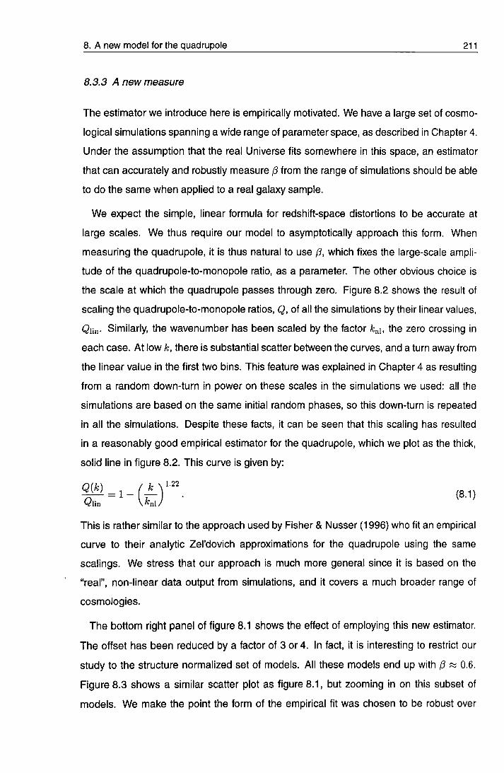
8. A new model for the quadrupole 211
8.3.3 A new measure
The estimator we introduce here is empirically motivated. We have a large set of cosmo-
logical simulations spanning a wide range of parameter space, as described in Chapter 4.
Under the assumption that the real Universe fits somewhere in this space, an estimator
that can accurately and robustly measure p from the range of simulations should be able
to do the same when applied to a real galaxy sample.
We expect the simple, linear formula for redshift-space distortions to be accurate at
large scales. We thus require our model to asymptotically approach this form. When
measuring the quadrupole, it is thus natural to use p, which fixes the large-scale ampli
tude of the quadrupole-to-monopole ratio, as a parameter. The other obvious choice is
the scale at which the quadrupole passes through zero. Figure 8.2 shows the result of
scaling the quadrupole-to-monopole ratios, Q, of all the simulations by their linear values,
Q i i n . Similarly, the wavenumber has been scaled by the factor fcni, the zero crossing in
each case. At low k, there is substantial scatter between the curves, and a turn away from
the linear value in the first two bins. This feature was explained in Chapter 4 as resulting
from a random down-turn in power on these scales in the simulations we used: all the
simulations are based on the same initial random phases, so this down-turn is repeated
in all the simulations. Despite these facts, it can be seen that this scaling has resulted
in a reasonably good empirical estimator for the quadrupole, which we plot as the thick,
solid line in figure 8.2. This curve is given by:
« * > = l - f A V " . (8.1) Qlin \knl.
This is rather similar to the approach used by Fisher & Nusser (1996) who fit an empirical
curve to their analytic Zel'dovich approximations for the quadrupole using the same
scalings. We stress that our approach is much more general since it is based on the
"real", non-linear data output from simulations, and it covers a much broader range of
cosmologies.
The bottom right panel of figure 8.1 shows the effect of employing this new estimator.
The offset has been reduced by a factor of 3 or 4. In fact, it is interesting to restrict our
study to the structure normalized set of models. All these models end up with p ^ 0.6.
Figure 8.3 shows a similar scatter plot as figure 8.1, but zooming in on this subset of
models. We make the point the form of the empirical fit was chosen to be robust over

8. A new model for the quadrupole 212
0.5
0
-0.5
Tm—m—I—r—r
J I L I I I I
0 0.2 0.4 0.6 0.8 1.2
Figure 8.2: The scaled quadrupole-to-monopole ratio for all the simulations and bias models described
In Chapter 4. The y-axis is scaled to the expected, linear theory value of Q, the x-axis is scaled to the
zero-crossing scale of the quadrupole, feni.

8. A new model for the quadrupole 213
0 . 5 0 . 5 5 0 . 6 0 . 6 5 0 . 7 0 . 5 0 . 5 5 0 . 6 0 . 6 5 0 . 7
( i i 0 . 5
0 . 3
0 . 7
0 . 6
0 . 5
0 . 4
0 . 3 h
( ^ - ^ i r u e ) = - 0 - 1 4 2
a= 0 . 0 4 1
I I I I I I I I I I I I M I I I I I I I I 1
Pairwise
( ^ - / ^ i r u e ) = - 0 . 1 0 7 a= 0 . 0 4 6
I I I I I I I I I I I I I I I I I f I I I I
I I I I I I I I I I I I I I I I I I I I J I I J I I i.
E x p o n e n t i a l
( / ? -^t .ue> = - 0 . 1 2 5
0 = 0 . 0 4 4
M I I I I I I I I I I M I I M
New model
( ^ - ^ t r u e > = - 0 . 0 3 5 (7= 0 . 0 5
I I I I I I I I I r I I I I I I I I I I I I I I I I
0 . 7
0 . 6
0 . 5
0 . 4
0 . 3
0 . 7
0 . 6
0 . 5
0 .4
0 , 3
0 . 5 0 . 5 5 0 . 6 0 . 6 5 0 . 7
^6
0 . 5 0 , 5 5 0 . 6 0 . 6 5 0 . 7
Figure 8.3: The same as figure 8.1, but including only the structure normalized simulations. These all have
(3 « 0.6, enabling us to zoom in on this area of parameter-space. Bias prescriptions have the same point
type as in figure 8.1, model 1 (stars), 2 (crosses), 3 (circles), 4 (open squares), 5 (solid triangles), 6 (open
triangles), and 7 (solid squares).

8. A new model for the quadrupole 214
a very wide range of cosmological parameters. If one requires a fit to only a particular sub-class of models, an even less biased estimator could be defined.
8.3.4 Scatter in the relationship
There are two sources of scatter in the curves we have looked at (figures 8.1 and 8.3):
• Bias model. Different prescriptions for biasing the galaxy catalogues result in sys
tematically different best-fit values of p, even though they are constrained to have the
same values of crf^', and hence ^ s - This is demonstrated in figures 8.4 and 8.5.
• Random. The simulations are of finite volume, and thus do not completely measure
the power spectrum. This causes a random scatter. The process by which the
simulations are biased involves the random (Poisson) sampling of the density field
to create a galaxy field, and this stochastic effect also causes estimates of p to scatter
around their mean value. This random scatter is shown in figure 8.6.
As well as reducing the systematic offset caused by using a poorly fitting model for the
distortions, we would also like to use a statistic that minimizes the internal scatter from
these sources.
The conventional method for describing the bias factor, b, is by the ratio of as in the
galaxy and the mass fields. In the approximation that both power spectra have the
same shape, or at least the same shape on scales that contribute to the fluctuations
in %h~^ Mpc spheres, this is equivalent to a boost in the galaxy power spectrum nor
malization by a factor I? relative to the mass spectrum. Most physical prescriptions for
galaxy formation, in contrast, result in a bias that is to some extent scale dependent
(Mann, Peacock, & Heavens 1998). For example, the large scale galaxy distribution may
have a constant bias, but this may be reduced in clusters where the number density is
sufficiently high that a significant amount of merging has occurred.
In figures 8.4 and 8.5 we show the four simulations that have the widest range of biasing
schemes. The E3S simulations have been biased using all seven schemes described in
Chapter 4, and the L3S and 04S cosmologies have been biased using six out of the
seven. The left hand panels show the scatter of Pf,i with p^. As can be seen, for any
one simulation, most of the biasing prescriptions result in the same values of p^: not
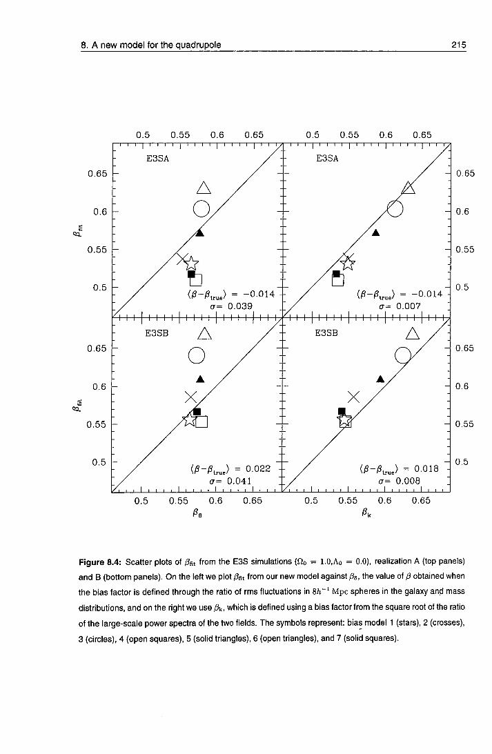
8. A new mode l for the quadrupo le 215
0 . 6 5
0 .6
5a.
0 . 5 5
0 .5
0 . 6 5
0 ,6
0 .55
0 .5 h
0 .5 0 . 5 5 0 .6 n—I—I—I—n—I—I—I—1—I—I—I—I—r
E3SA
< ^ - ^ t r u . ) = - 0 0 1 4 (7= 0 . 0 3 9
I I I I I I I I I I I I I I I I
(^ - /3 t .ue) = 0 . 0 2 2 t7= 0 . 0 4 1 (T= 0 ,008
0.5 0 ,55 0.6 0 .65 T—I—I—I—I—I—I—I—i—I—I—i—I—I—I—I—I—I—i—I—r
E3SA
(/3-/3irue) = - 0 0 1 4 a= 0 . 007
I I I I I I I I I I I I I I M I I I I I I
0 .65
0.6
0 .55
0.5
0 .65
0,6
0 ,55
0,5
0 .5 0 .55 0 .6 0 .65
^8
Figure 8.4: Scatter plots of /3fit from the E3S simulations (Qo = l.O.Ao = 0.0), realization A (top panels)
and B (bottom panels). On the left we plot /3fit from our new model against I3&, the value of 0 obtained when
the bias factor is defined through the ratio of rms fluctuations in 8/i~' Mpc spheres in the galaxy and mass
distributions, and on the right we use /3k, which is defined using a bias factor from the square root of the ratio
of the large-scale power spectra of the two fields. The symbols represent: bias model 1 (stars), 2 (crosses),
3 (circles), 4 (open squares), 5 (solid triangles), 6 (open triangles), and 7 (solid squares).

8. A new mode l for the quadrupo le 216
0.45 0.5 0.55 0.6 0.65 0.45 0.5 0.55 0.6 0.65
0.65
0.55 h
^ 0.65
H 0.6
H 0.55
0.45
0.65
H 0,45
0.65
(P-KJ = - 0 . 0 6 a= 0.05
iP-^rJ = - 0 069 (T= 0.054
0.45 0.5 0.55 0.6 0.65 0.45 0.5 0.55 0.6 0.65
0.55 h H 0.55
0.5
0.45 h H 0.45
Figure 8.5: The same as figure 8.4, but for the L3S (fio = 0.3,Ao = 0.7) and 04S (Qo = 0.4, Ao ^ 0.0)
simulations.

8. A new mode l for the quadrupo le 217
really surpr is ing since most of them were fixed to reproduce clustering on these scales.
There is, however, a significant scatter in the values of ^ f i t for these different biases. In
order to el iminate this scatter, on the right hand panel in each case we plot Pf^ against
/3k, where /3k is obta ined using the bias factor derived from the ratio Pga\ik)/Pmass{f^) at a
f ixed value of k. Ideally, we would like to use the smallest value of k possible, to reflect
the asymptot ic value of the bias. In practice, we f ind that the large uncertainty in the
power spect rum at large scales, caused by the small number of modes to average over,
produces its own scatter in the deduced bias. We f ind the value of k that minimizes the
scatter '\s k = 0.07272hMpc~^. Use of /3k rather than has a dramatic effect on the
scatter of the different models, pull ing them much closer to the (3 = /3fit line. The scatter
is reduced by a factor of five in the ESS models and around two in the \ovj-n models.
0.6
0 .58
^= 0 . 5 6
0 . 5 4
0 . 5 2
0 . 5 2 0 . 5 4 0 .56 0 .58 0.6 0 .52 0 .54 0 .56 0 .58 0.6 T—I I I r
M o d e l 1 M o d e l 1
(/S-/Strue) = - 0 0 0 3 a= 0 . 0 1 8
( / 3 - / ? i r J - 0 .013 - I CT= 0 .018
I I I I I I I I I I I . I I I I I I 1
0.58
0.56
0 .54
0 .52
0 . 5 2 0 . 5 4 0 . 5 6 0 .58 0.6 0 .52 0 .54 0 .56 0 .58 0.6
Figure 8.6: The scatter of /3fit for the ten independent E3S simulations with bias model 1. This scatter thus
reflects the intrinsic random scatter between simulations with different initial phases and different Poisson
sampling to obtain the galaxy distribution.
In f igure 8.6 we look at true random scatter by comparing the values of /3 from the ten
independent E3S simulat ions biased with model 1. This represents the intrinsic scatter.
We see that changing the definition of Ptme has no effect in this case. The resultant
scatter of around 3% is thus the lowest uncertainty we could place on /3 by measuring it

8. A new model for the quadrupole 218
f rom one of the simulat ions. In the next section, we will use these methods to analyse p
f rom the mock catalogues. Since the mocks have been constructed from the simulations,
they contain no extra information, and there is no way of determining /3 more accurately.
8.4 Appl icat ion to mock cata logues
We now at tempt to apply this model for the velocity dispersion directly to mock catalogues,
as if they were real datasets. The problems of deal ing with the survey window function
in terms of its effect on the quadrupole itself and on the error on this quantity have
been d iscussed in Chapter 7. Here, we will compare the est imated uncertainty on /?
der ived previously with an est imate from measuring ^ in ten mock surveys drawn from
independent A/-body simulations. We choose to apply the technique to the 2dF South
Galact ic slice in an J o = 1. structure normalized model .
8.4.1 A consistent approach
For the compar ison to be worthwhi le, we must take pains to ensure that the implemen
tation of the two different methods is as similar as possible. There are several key
considerat ions that must be dealt wi th.
• T h e distant observe r approximation. As noted in Chapter 7, the linear theory
formal ism of Kaiser (1987) is applicable only when the redshift-space density field
can be approximated as a sum of plane waves, so it will not work for surveys of large
opening angle where this criterion is not met. Whilst there do exist methods of dealing
with wide angle surveys in one go by expanding the density into spherical harmonics
(Heavens & Taylor 1995), we do not concern ourselves with those here. Rather, we
split the survey up into separate angular bins with relatively small opening angle, and
treat each one with the plane parallel approximation. For the 2dF SGP geometry the
decl inat ion range is 15°. It thus seems reasonable to pick a right ascension range for
our angular bins of comparable extent. The azimuthal extent of the South Galactic
strip is w 90° cos 30° = 78°. We split the survey into three bins each spanning 26°
in right ascension. Note that there are pairs of galaxies that span adjacent bins
but still have opening angle less than the 26° bin width. To avoid throwing this data
away, we also include the two overlapping bins. The effect of a finite opening angle

8. A new mode l for the quadrupo le 219
on the est imated value of ^ has been studied by Cole, Fisher, & Weinberg (1995). From their f igure 8 it is clear that a 26° opening angle should only result in a one percent underest imate of the quadrupole-to-monopole ratio of the power spectrum. Since Q\m{P) is approximately linear over a reasonable range of /3, this introduces negligible systematic error. We thus perform our analysis for five bins of angular extent ^ 26° x 15° and average the resulting power spectrum estimates. The method of random realizations descr ibed in Chapter 7 is not affected by the distant observer approximat ion, but to make the treatment equivalent, we also split the survey into the same five angular bins. The bins sample a density field from the the same initial phases, and the results are combined incoherently, as described for the NGP and SGP in sect ion 7.6.3.
• Power at d iscre te k va lues . Our mock 2dF catalogues have been drawn from N-
body simulat ions that have been carried out on a finite, periodic grid. When the
initial d isplacements are appl ied to the dark matter particles, power is given to the
density f ield only at modes that are at discrete wavenumbers, integer multiples of
the fundamenta l mode of the simulation cube. On small scales, non-linear evolution
between the modes will result in the effective " leakage" of power from these modes.
On large scales, this will not be the case, and to use a box for the Fourier analysis that
is not equal to the the size of the original simulation cube will result in the sampling
of modes that do not have a well def ined amplitude. We thus restrict our analysis
to a cube that has the length as the original simulation, L B O X = 345.6/i-^ Mpc (see
sect ion 4.7) .
• Non-l inear mode coupl ing. In the simulations, as in reality, gravitational instability
causes non-l inear evolution of the density field such that it is no longer a good ap
proximation to assume there is no "cross-talk" between nearby modes. Correlations
are thus introduced between the modes on top of those caused by the convolution
with the survey window funct ion. On the largest scales, this result is expected to be
negligible in compar ison to the smoothing introduced by the window function, since
the modes are still in the linear regime. As we extend to smaller scales, the effect
of the w indow funct ion in correlating nearby modes is constant: see figure 7.6. The
non-l inear behaviour gets stronger at smaller scales, so eventually the effects must
become comparable, and on yet smaller scales the coupl ing effect will dominate.

8. A new mode l for the quadrupo le 220
Prel iminary work on this topic (Meiksin & White 1999) suggests that it could be an issue on the scales (below the zero-crossing) that we consider, but the extent of the problem is highly dependent on the ampli tude of the power spectrum used. The effect is likely to be even worse in redshift space than in a real-space N-body simulation, since virial velocit ies stretch out physically small non-l inear structures (clusters), inevitably spreading information that may be localized in real-A;-space over a range of scales in redshift-A;-space. We make no attempt to introduce non-linear coupling into the random phase method of Chapter 7, which we have shown to be largely model-independent.
• T h e z e r o - c r o s s i n g s c a l e . The velocity dispersion in the simulations is such that
kni « 0 . 3 / i M p c " ^ We model the same zero-crossing in the model power spectrum
used to obtain the mode ampli tudes by using a painwise exponential model for the
velocity distr ibution with dispersion = 500km s " ^
8.4.2 The true error
Having made the two methods as equivalent as possible, in advance of the analysis we
now consider reasons why the errors derived on the clustering using these techniques,
even if they agree with each other, may not accurately reflect the true error on (3 from a
redshift su rvey
• Fundamenta l wavelength. Related to the point about discrete wavenumbers made
above, we note that by restricting the wavenumbers examined, we also limit the use
fulness of the survey for studying large-scale modes, because there is no wavelength
longer than L B O X - In order to again make the two treatments identical, we will also
apply the random phase method to a box of the same size. Note that, especially in the
case of a large survey with volume much greater than the size of this cube, this will not
accurately reflect the real ability to measure the power spectrum on large scales, and
will hence lead to an over-prediction of the uncertainty on parameters like /3 which rely
on long-wavelength information to pin them down. In the next section we will assess
the size of this effect by compar ing the random phase method appl ied to a grid of
LBOX = 345.6/ i -^ Mpc with results f rom a much larger cube.

8. A new mode l for the quadrupo le 221^
• T h e distant observe r approximation. As mentioned above, we combine our angular bins incoherently, ie. we do not measure power picked out by pairs of separation greater than 2 6 ° . If the method of spherical harmonic decomposit ion, or indeed any other technique that does not rely on the plane-parallel expansion, can be applied to the data set in the same way, there is no need for this caution, and the value of (3 will be measured to rather greater accuracy Assuming this is the case, we will quantify the size of this improvement by compar ing the error from the random phase method appl ied to the five bins with the same technique appl ied exactly as in Chapter 7, ie. to the whole 2dF South Galactic strip in one go.
• T h e z e r o - c r o s s i n g s c a l e . As pointed out in Chapter 7, real galaxy catalogues have
general ly found rather smaller velocity dispersions than the ones measured from N-
body simulat ions. This will again push the zero-crossing of the quadrupole out to
higher k, giving a wider range of scales for which there is a reliable model of the effect
of the non-linearity. Again , this increase in accuracy can be anticipated by using the
random phase method with a more observationally realistic velocity dispersion.
• Redshi f t to phys ica l coordinates. The conversion from redshift to true distance
depends on the evolution of the expansion factor, which is a function of the geometry
of space-t ime, ie. dependent on Q.Q and AQ. Using the wrong values of these quantities
in the coordinate transform will result in a bias in the anisotropy of the power spectrum.
It is this bias that results in the so-called "cosmological" redshift-space distortions
investigated by Nakamura, Matsubara, & Suto (1998). This is, in general, only a
signif icant effect at redshifts comparable to unity; at low z, the translation is linear and
not sensit ive to the cosmology The magnitude of the bias will have to be assessed
when deal ing with the real catalogues, since they do have appreciable depths. For
this t reatment we simply use the known value of QQ = 1 from the simulations to make
the conversion, el iminating this bias.
8.4.3 The expected error
In this sect ion we apply the formal ism of the previous chapter to estimate how well we
should be able to measure cosmological parameters from the 2dF South Galactic strip.
As ment ioned above, we use a model power spectrum with = 500km s"^ to accurately
model the zero-crossing of the quadrupole. Our standard model has ^ = 0.55, which

8. A new mode l for the quadrupo le 222
is the value we expect to obtain f rom the simulations, as demonstrated in figure 8.6. W h e n we perform our analysis on a grid of LBOX = 345.6h~^ Mpc, the same size as the fundamenta l cube of the simulat ions, we f ind an expected, 1-a error on /3 of 18%. As far as possible, we have made this analysis consistent with the analysis of the "real" mock catalogues presented below. If we perform the analysis using a larger cube^ we find the error sl ightly reduced, to 15%. The reduction is minimal, as the window function for one angular division of the survey has a width comparable to the spacing of the modes on the fundamenta l gr id. There is thus little to be gained in increasing the resolution.
This is for the survey split up as descr ibed above. Assuming the spherical harmonic
method preserves all information, we can simulate this by running the model without
splitt ing into angular bins. The resultant error on 13 will be lower because we can use
more pairs at w ide angular separat ion to probe the long-wavelength modes. We find an
expected error of 11% for the case where we combine a larger box-size with use of the
whole survey.
8.4.4 The measured PS
In f igure 8.7 w e plot the monopole power spectra and quadrupole-to-monopole ratios
measured f rom the ten independent A/-body mock catalogues. It can be seen that the
mocks are general ly in good agreement with each other, but that there is a considerable
degree of scatter between the realizations, especially on large scales. As we predicted in
sect ion 7.5, Q{k) is substantial ly less wel l-determined than the monopole power.
We use a two-parameter least squares fit to obtain values of /3 and kni from each
of the ten mock catalogues. This fit employs the covariance matrix found using the
random realization method of Chapter 7. The model used in the fit is that described
in sect ion 8.3.3, which was found to be an unbiased estimator of (3 for the full simulation
cubes f rom which the catalogues have been drawn. In the full simulation cubes, we
used the method of multiple ZeI'dovich runs to measure the expected error on Q{k) as a
funct ion of scale. Effectively, then, we had a covariance matrix that had all off-diagonal
e lements set to zero. Here, we need to deal with correlations between modes due to the
^ We use a 3x fundamental cube, ie. L B O X = 1036.8/i~^ Mpc, larger than the limiting radial distance of
the volume limited sample considered.

8. A new model for the quadrupole 223
3 . 5
0 . 5 h
1.5 - 1 - 0 . 5
L o g i o [ k ( h M p c - i ) ;
Figure 8.7: Power spectra, Pik), and quadrupole-to-monopole ratios, Q{k), for the ten independent mock
2dF catalogues, each constructed from simulations with the same cosmology and bias prescription.

8. A new mode l for the quadrupo le . 224
survey w indow funct ion, and to model this we use the non-diagonal covariance matrix obta ined in the previous section with the method of multiple random realizations.
We measure the average value of p over the ten simulations, and the standard deviation
between the est imates. We f ind Pa,y - 0.493 ± 0.173. Note that the standard error on the
mean , since we have ten realizations, is 0 .173 / \ / l 0 = 0.055. The measured mean is
approximately 1-a discrepant from the true value (/? « 0.55, from figure 8.6), and so our
model is not signif icantly b iased. The scatter on p, however, is around 35% of the mean;
this is far in excess of the 18% error we expect from the previous section. We now address
the quest ion of the discrepancy between the two estimates.
Figure 8.8 shows the fractional error on P{k) the absolute error on Q{k) as a function
of scale. We compare the variance we get from the ten independent realizations with
the "expected" relationship f rom applying the random phase method to the same survey
geometry. The correspondence between the two methods is clear; the random phase
method has not under-predicted the degree of uncertainty on the distortion of each
individual mode.
We conclude that the reason for underestimating the error must be that there exist
ser ious correlat ions between the data points in addition to those due to the shape of the
survey w indow funct ion, which we have taken into account. If the correlations do not
come f rom the convolution with the window function, and they are not modelled by the
l inear t reatment of the random phase method, they must be caused by non-linear effects
that invalidate our use of a Gaussian density field. It was pointed out in section 8.4.1
that non-l inear evolution of the small-scale density modes introduces coupling between
them, which w e fail to take into account in using the random phase method, but which is
implicit in the N-body method which has fol lowed the evolution of these modes accurately
It will be seen f rom figure 3.2 that the dimensionless power spectrum from the Oo = 10 ,
structure normal ized simulation has an ampli tude of around lO*^-^ at the zero-crossing of
the quadrupole, which occurs at around k = 0.3. Given that the bias factor on these
scales is 6 « 1.8, the value of the mass power spectrum ampli tude at the zero-crossing
is 10°-^/62, approximately unity. Thus, the approximation that the modes are uncorrelated
wh ich , as shown in Appendix A, is true only when the ampli tudes are much smaller than
unity, is broken, and we should not be surprised that some mode-coupl ing has occurred.

8. A new model for the quadrupo le 225
• 0 . 5
o
o b
O
- 1 . 5
0
- 0 . 5
o
- 1
"T 1 i 1 1 1 1 1 1 i i 1 1 i r
_i I I L
- 2 1.5 - 1 - 0 . 5
L o g i o [ k ( h M p c - i ) ;
0
Figure 8.8: Fractional error on the power spectrum (upper panel) and absolute error on the
quadrupole-to-monopole ratio (lower panel). The solid line is from the variance between then ten inde
pendent mock catalogue realizations of the survey, the dotted line is from applying the random phase
technique of Chapter 7. To both curves we have Poisson errorbars to the points using the relation that
the standard deviation of the scatter is given by ass = (Ts/y/2{N - 1), where CTS is the measured scatter from
N realizations (Barlow 1989).

8. A new mode l for the quadrupo le 226
Figure 8.9: Covariance matrix from then ten indpendent mock catalogues. We have smoothed with a boxcar
smoothing of width three cells. We have also normalized, as in figure 7.6, such that the \k - k'\ =0 modes
have unit variance.
In figure 8.9 we show a similar covariance matrix to that in figure 7.6, only this one
has been calculated from the ten independent mock catalogues. The use of only ten
realizations, as opposed to the one hundred used in the random realization method,
introduces noise in estimates of the covariance; we have removed some of this noise by
smoothing the matrix in two dimensions, simply to make the effect of non-linearities more
visually obvious. The decrease of the signal over the noise is quite clear as we progress
to smaller scales (towards the bottom right-hand corner of the figure).
Quantifying the extent of this effect is a far harder task than showing it is significant. Just
as we use one hundred random realizations to obtain the covariance matrix introduced
by the survey window function, Meiksin & White (1999) use one hundred A/-body simu
lations to examine the extent of correlations between the modes. This is an extremely
time consuming job, and it is difficult to see how this could ever be practically used in

8. A new mode l for the quadrupo le 227
an iterative way to est imate the strength of the coupl ing. The ampli tude of the power spect rum, which has general ly been irrelevant to us since it drops out of the quadrupole-to-monopole ratio, is now an important additional factor in determining the strength of the effect. Meiksin & Whi te also introduce a faster procedure of using repeated Zel'dovich approximat ion runs to achieve the same goal, but they f ind that this method underestimates the correlat ions since shell-crossing occurs, and key sources of non-linearity, ie. galaxy clusters, cannot be model led accurately
8.5 C o n c l u s i o n s
Are we left to conclude, then, that the 2dF survey will not be able to measure p much
more accurately than 3 5 % ? If the coupling between modes is significant, developing a
model that can follow the quadrupole-to-monopole ratio out to higher wavenumber is of
little use. There are diminishing returns, since the modes are more and more correlated
as we progress to smaller scales.
We have al ready seen that the width of the 2dF window function is such that using a
longer box length is broadly irrelevant. We do, however, note that, if there is less to be
ga ined in pushing to smaller scales, the shot-noise on these scales is less relevant. We
could then choose to select a deeper volume limited sample that will determine longer
wavelength modes rather better, with a narrower window function, at the expense of
more noise on small scales. Alternatively we could use the whole magnitude limited
sample with an FKP min imum variance weighting scheme to optimize measurements of
the power spect rum at extremely large scales.
8.5.1 Reducing non-linearities
In the random realizations method, we have assumed a convenient form for the net effect
of non-l inear velocity dispersion on the power spectrum. Whilst this is, on aggregate,
a val id approach, in a real survey or an A/-body simulation this is not how non-linearity
comes about ; the coupl ing between fc-modes is a local effect in r-space, it takes place
inside part icular non-l inear structures, ie. rich clusters. In these volumes, mode coupling
is extremely strong. As pointed out in Chapter 6, if we can somehow excise these regions
f rom our t reatment, we could not only create a better behaved, more linear quadrupole-

8. A new mode l for the quadrupo le 228
to -monopole ratio, but have an even more dramatic effect in lessening the correlations between modes on these scales. This could be achieved by the identifying and removing the signal f rom clusters, as descr ibed in Chapter 6, or perhaps by performing the distort ion analysis in r -space, by looking at the correlation function ^(cr ,7r) . The spatially localized effect can be removed as it involves close transverse pairs.
8.5.2 Future surveys
It may prove difficult to deal with clusters accurately since identifying them robustly in
redshift space with a select ion function is a complex issue (Moore, Frenk, & White 1993).
If these diff iculties cannot be overcome, then we may have to turn to larger surveys to
accurately measure p. Large-scale modes are at a premium, because:
• The w indow funct ion convolution is less significant if the volume is large.
• The redshif t-space distort ions are more close to their linear theory values.
• Non-l inear mode-coupl ing will not be significant.
The f inding of Heavens & Taylor (1997) that "width is better than depth" implies that
a wider angle survey like the SDSS may be more efficient, even for a subsam-
ple that conta ined the same volume as 2dR This strategy also lessens the poten
tial contaminat ion f rom evolut ionary effects and cosmological redshift-space distortions
(Ballinger, Peacock, & Heavens 1996; Matsubara & Suto 1996).
Finally, given the diminished relevance of the shot-noise if substantial correlations
exist o n smal l scales, a high number density of galaxies is not relevant. There is little
to be lost, then, in a sparse sampl ing strategy Heavens & Taylor (1997) find that the
opt imum sampl ing fract ion, / , is given by f P = 500/ i"^ Mpc^, where P is the power at
the wavelengths of greatest interest. In the standard model , outl ined in Chapter 2, we
expect to see the power spectrum turn over to the Harrison-Zel'dovich regime. Thus the
power will decrease at the largest scales. To measure the very longest modes, sparse
sampl ing is therefore not useful, but, referring to figure 2.5, it can be sen that the galaxy
power spect rum is a long way f rom zero at the longest scales probed by the APM survey
To really constrain the power spectrum in three dimensions at the scale probed by COSE,
8. A new mode l for the quadrupo le 229
we shou ld opt imize our estimation for P « 2000h~^ Mpc^ The desirable characteristics of a survey specif ically designed to measure /3 and nothing else might be:
• Large vo lume, to minimize convolution effects and non-linearity.
• Wide angular coverage, like PSCz, or 6dF, to measure large-scale power accurately
and avoid contaminat ion by evolutionary effects.
• Sparse sampl ing at a rate of roughly one-in-four, to measure long wavelength modes
with max imum eff ic iency
• Sharp ly peaked select ion funct ion, such that it is efficient for constructing a volume-
l imited sample.
R e f e r e n c e s
BallingerW. E., Peacock J. A., Heavens A. F, 1996, MNRAS, 282, 877
Barlow R. J., 1989, Statistics: a guide to the use of statistical methods in the physical sciences, Manchester
physics series. Wiley
Cole S., Fisher K. B., Weinberg D. H., 1995, MNRAS, 275, 515
Fisher K. B., Nusser A., 1996, MNRAS, 279, L1
Heavens A. F., Taylor A. N., 1995, MNRAS, 275, 483
Heavens A. F, Taylor A. N., 1997, MNRAS, 290, 456
Kaiser N., 1987, MNRAS, 227,1
Mann R. G., Peacock J. A., Heavens A. F, 1998, MNRAS, 293, 209
Matsubara T , Suto Y , 1996, ApJ, 470,1
Meiksin A., White M., 1999, MNRAS, submitted, astro-ph/9812129
Moore B., Frenk C. S., White S. D. M., 1993, MNRAS, 261, 827
Nakamura T T , Matsubara T , Suto Y., 1998, ApJ, 494,13
Peacock J. A., Dodds S. J., 1994, MNRAS, 267,1020

Chapter 9
Conclusions and further work
THE ARGUMENT We summarize the conclusions of the preceding chapter, and
outline some directions for future work to take.
The focus of this thesis has been to develop techniques to estimate fundamental cos
mological quanti t ies f rom redshift surveys, especially f rom the ongoing Anglo-Australian
2dF, and the US Sloan Digital Sky Survey projects. These two surveys, the most ambi
t ious ever in the area of large-scale structure, will open up a new era of high precision
measurements in cosmology In particular, the large volumes they probe will enable us,
for the first t ime, to directly compare the clustering of galaxies with the amplitude of the
m a s s f luctuat ions on the scales measured by COBE. The relationship between these two
is fundamenta l to our understanding of galaxy formation.
In order to fully anticipate the arrival of such high quality data as the new surveys
will provide, the use of mock catalogues that roughly mimic the selection functions and
likely cluster ing of the real data is crucial. The suite of mocks we present in Chapter 4
is enormous ly useful for this, but is still restricted in many ways. A key future goal is
to incorporate semi-analyt ic models (SAMs) for galaxy formation. SAMs are a powerful
method for producing "realistic" galaxies with types, magnitudes, colours etc., without
recourse to ultra-high resolution N-body simulation. They thus enable us to create big
s imulat ions that sample large-scale modes of the power spectrum, contain fair samples of
clusters, and simultaneously contain a physically motivated bias between the galaxy and
mass f luctuations. Ideally, we would like to increase the volumes beyond even those used
in our catalogues, avoiding potential problems that arise due to periodicity and lack of k-
space resolution that we discuss in Chapter 8. As discussed in Chapter 4, using large
simulat ions like the Hubble volume as the source for our mocks allows us to incorporate

9. Conc lus ions and fur ther work 231^
the effects of evolution very simply, since the simulation is output along the observer's light cone. This will be especially useful for modelling the deep surveys such as VIRMOS and DEEP, discussed in Chapter 1, that will be sensitive evolutionary probes.
The incorporation of non-cosmological effects in our catalogues has been illustrated
in Chapter 5 where we examine the effect of Galactic dust on the clustering signal in
the SDSS. It will be of great interest to extend this treatment to the APM catalogue, and
hence the 2dF, and retrospectively the Stromlo-APM to see if this was at all biased.
Other planned or current uses for the mock catalogues include:
• Looking at cosmetic problems in the real catalogues, eg. errors due to the finite
spacing of fibres.
• Studying the cosmological redshift-space distortions that arise when the wrong cos
mology is used to convert the catalogue from redshift- to real-space.
• Calculating at what level the new catalogues will be able to discriminate against a
fractal distribution of clustering, ie. large-scale departures from homogeneity.
One of the chief statistics we have employed has been the quadrupole-to-monopole
ratio of the redshift-space power spectrum. This quantity is especially useful because, in
the regimes considered, it is not directly sensitive to the amplitude or shape of the power
spectrum. We have demonstrated in Chapter 6, by comparison with N-body results,
that existing models for the redshift-space distortions, especially as measured via the
quadrupole estimator, are inaccurate and can lead to substantial bias if applied to a large
dataset. The exponential and Gaussian models for non-linear velocity dispersion do not
generally replicate the shape of the curve on large scales, and the Zel'dovich approxima
tion breaks down if there is a high velocity dispersion or a significant bias. In Chapter 8
we have extended this treatment to a much larger sample of different cosmologies and
shown that, of the simple analytic forms for the correction to the power spectrum, the one
that matches most closely is that of a painwise exponential. We find from our simulations
that this still provides a biased estimate of the /3-parameter, and introduce our own, purely
empirical relationship for the non-linear correction as a function of scale, which is shown
to be unbiased, ie. the systematic differences are less than the intrinsic scatter.
The importance of accurate error estimation cannot be over-stressed. Scientific re
sults are meaningless without it, since comparisons cannot be made between different

9. Conc lus ions and fur ther work 232
datasets without a reliable estimate of the relative accuracy of each. Our technique, of using repeated realizations of Gaussian random fields for the density, is outlined in Chapter 7. The comparison with our mock catalogues in Chapter 8 serves to confirm the validity of this treatment, demonstrating that it provides an accurate assessment of the error on derived parameters due to the finite volume contained within a given survey geometry. We consider that this technique will be a useful tool in optimizing the design of future galaxy redshift surveys.
On the whole, the immediate results of applying this treatment to the new generation
of surveys are encouraging; but it transpires that a simple application to the data will not
be able to constrain the power spectrum, especially on large scales, as accurately as we
would wish, and errors on the key parameter ^ are significantly larger than anticipated.
However, in Chapter 6 we applied one method in particular to our A/-body simulations that
was effective at removing much of the non-linear signal from the quadrupole estimator.
This is the method of cluster collapse, which prevents these highly non-linear structures
from contributing to the power spectrum and hence washing out the linear signal. We
have high hopes for this method, but it remains to make a detailed study of its application
to real surveys conducted in redshift-space. The ability to define cluster membership here
is complicated by the smearing caused by the radial velocities within the clusters, and by
errors in the selection function which is estimated from the dataset itself. Developing
optimal methods for choosing the parameters of an anisotropic friends-of-friends search,
and assessing the biases that may result from it, is another potential application of our
mock catalogues.
A further possible refinement is to include non-linear effects in the covariance matrix
used in fitting a model to the data. This introduces a further degree of complexity as
these effects are sensitive to the amplitude of the underlying mass power spectrum, and
currently they can only be measured by repeated A/-body simulation. It is not unlikely
however, that further study will produce a simple empirical model for the degree of
correlation between two modes as a function of scale and a^^. This would be very
easy to include in our treatment, by convolving the covariance matrix we obtain from the
survey geometry effect with that which arises from non-linear coupling.
The final conclusion then is that, to really constrain cosmological parameters, we must
probe long wavelengths accurately, or refine techniques for removing small-scale non-

9. Conc lus ions and fur ther work 233
linearities from the data. These methods must be further developed and tested before being applied to data from the new generation of redshift surveys currently in progress.

Appendix A
Linear theory
T H E A R G U M E N T We present the derivation of the linear theory for the
growth of density perturbations which is the keystone of much of the work
in this thesis.
A.I Introduction
Throughout this work, we have used the power spectrum of density fluctuations as an
important probe of the cosmological parameters. In this appendix we briefly outline the
steps in deriving the linear growth of fluctuations with time.
A.2 Three equations
The whole of linear theory is based on three simple equations that are familiar from all
branches of physics:
• First, the continuity equation, which simply states that the rate of change of density in
a box is proportional to the rate of flow of matter out of it, in the absence of sources or
sinks,
|e + v . ( p v ) = 0 (A.I)
• Next, the Euler equation relates the rate of change of momentum in a fluid to the
potential gradient,
^ + (v .V)v = -V(j> (A.2)

A. Linear theory 235
• Lastly, Poisson's equation relates the second derivative of the gravitational potential to
the underlying density.
(A.3)
A.3 Comoving co-ordinates
We define a physical co-ordinate, r, such that r = a(i)x, where x is the co-moving co
ordinate. The physical velocity, v, is thus v = r = ax + ax. This represents the Hubble
expansion velocity with peculiar velocity superimposed. The co-moving peculiar velocity
is u = X . We begin this derivation by transforming the three equations above into co-
moving co-ordinates. As r ^ x,
V, a{t)
The chain rule for partial differentials states:
d d dx d dt r dt -
X ' 'di r dx
Now, from our definition of x.
ax
dt
so
d_ dt
a a = - r ^ = - X - ,
d_ dt
- - x V a
We will also employ the vector calculus identity:
V.((/)v) = 0V.V + v.V(j!>.
We define density fluctuations by
p(x,t) = § [ l + ^(x,t)].
(A.4)
(A.5)
(A.6)
(A.7)
(A.8)
(A.9)
These relations (equations A.4, A.7, A.8) are all we need to transform the continuity
equation (A.1) into comoving co-ordinates:
d5 dt
+ V .u + V.((5u) = 0 . (A.10)

A. Linear theory 236
Similarly for Euler's equation (A.2),
— + 2 - U + U V . U = 1-—- (A.11) at a a
Under a Friedmann-Robertson-Walker metric with no cosmological constant, conserva
tion of energy implies a = -GM/a?. Using the Poisson equation, we can write
V . ^ = 3 ^ = 4 . G p = - ^ . (A.12)
Here we have rewritten the potential as the sum of an averaged and a perturbed compo
nent, 0 = 0 + 0. Integrating both sides of the previous equation, we obtain
^ = - ^ . (A.13)
Substituting this value into equation A.11 yields
— + 2 - U + U V .u = ^ at a a
+ 2 " u + u(V.u) = - ^ . (A.14)
For the Poisson equation (A.3), we obtain
V20 a2
AnGpS. (A. 15)
A.4 Fourier space
In order to deal with the evolution of individual Fourier modes of the overdensity field, we
Fourier transform the three real space equations (A. 10, A.14, A. 15) into k-space. Any
field, 6, in real space can be written in terms of its Fourier components,
^(x) = ^ 0 k e x p ( - i k . x ) (A. 16) k
We use this relation to expand the cross-terms in equations A.10 and A.14,
/ ^ V.(u5) = V. 5 ] ^ 4 i e x p ( - i k i . x ) ^ U k 2 e x p ( - z k 2 . x )
\ ki k2
= ^ - i ( k i + k2)<5ki exp(-?(ki + k2).x) ki k2
= ^ ^ —ik(5k'Uk-k'exp(—ik.x) (A.17) k k'

A. Linear theory 237
Similarly,
u(V.u) = ^ U k i e x p ( - i k i . x ) ^ « k 2 . U k 2 e x p ( - i k 2 . x )
ki k2
ki k2 = 5 Z Z l ^ " k - k ' - ( k - k ' ) u k / e x p ( - i k . x ) . (A. 18)
k k'
If we Fourier transform equations A.10, A.14, and A.15, and substitute these results,
we obtain:
from the continuity equation
dt ^-ik.Uk-J2i^k'k.Uk-k'=0, (A.19)
k'
• from the Euler equation
^ + 2\k - E^^k'-i^ - k')ufc-.' = (A.20) ot a r j 0,
and from the Poisson equation.
^ = - 4 . G 4 . (A ,21 ,
These formulae are the Fourier-space analogues of the three equations we started with.
If we restrict ourselves to the linear regime where the fields have values much less than
unity, we can discard the summation terms in the above equations since they contain
products of two fields. Since the cross-terms have been thrown out, we have effectively
removed the coupling between modes with different wavenumber, and the modes will
evolve independently of each other.
A.5 Solutions
Keeping just the linear theory terms, we differentiate equation A.19 with respect to time
to get
Sk - ik.xik = 0. (A.22)
Now, combining the other two equations, A.20 and A.21, to eliminate ^,
. . . 2 ( ^ ) u . = - 4 „ G p f = -3*(5)| (A.23,

A. Linear theory 238
Multiply this equation by -ik,
-ik.Uk = 2i (^^^ k.Ufc - 3 (^^^ 4 . (A.24)
Substitute this result into equation A.22
4 + 2 i Q ) k . u , - 3 ( ^ ) j f c = 0. (A.25)
Finally from equation A.I 9, substitute ik.Uk = h
h + 2(-)Sk-3(-)s,=0. (A.26) \ a j \ a j
This is the general second-order differential equation for the linear evolution of the over-
density field, Sk-
In the special case of an Einstein-de Sitter Universe, a oc f^^, so
^ = V i and ^ = - | i - ^ (A.27) a 3 a 9
Looking for power-law solutions, 5 oc f", we obtain
6k = Akt'/' + Bkt-\ (A.28)
It can thus be seen that perturbations in the density field are superpositions of growing
and decaying states.
A.6 The peculiar velocity field
For the general case where the growing mode of the density field dominates, Sk =
AkD{t), we use the continuity equation (A.I9) to first order,
ik.uk = ^ = 6k^ = SkHf, (A.29)
where we define / = D/DH. Dividing by ik gives:
u , = -pkHf. (A.30)

A. L inear theory 239
Taking the inverse Fourier transform of this result gives us a relation between the peculiar velocity of a particle and its initial position, q:
u(q) = - H f - ^ J2 exp(-ik.q) (A.31)
This equation can then be integrated to calculate the displacement of particles from their
initial positions.
d(q,t) = fui<i)dt Jo
= | l E § ^ ^ - P ( - k . q ) . (A.32)
These final two equations describe the Zel'dovich approximation used in our simula
tions to give particles initial displacements and velocities from a set of Fourier amplitudes
Ak.
A.7 Redshift-space distortions
Under linear theory it is possible to derive a simple equation for the effect of the peculiar
velocity field on the observed clustering as measured by the power spectrum in redshift-
space (Kaiser 1987; Cole, Fisher, & Weinberg 1994).
p ^ ( s ) = / ( r ) Hr
1 ^ dU{r) (A.33) Hdr
The first factor comes from the effect of the peculiar velocity on the cross-sectional area
of the volume in question, the second from the expansion or compression in the radial
direction. Making the assumption of a distant observer sets the first term to unity, and in
the limit that \dU/dr\ < H, the radial term is well approximated by a first-order expansion,
and
/ ( s ) = / ( r ) ( l - i ^ ) . (A.34,
now, p/p = {1 + 6), so
l + S%s) = [l + 6^{v)](l-^^'^ (A.35)
Making the further assumption that j J^ c 1, this leads to
5^is) = S ^ r ) - ^ f . (A.36)

A. L inear theory 240
Now, the peculiar velocity field is given by equation A.31 above. This holds when Ak
is a perturbation in the mass density field. For a perturbation in the galaxy density field,
under the assumption of linear bias (js^' = M"^^), f{Qo) is replaced by /? = f{Q.o)/b.
The radial component of the velocity field is:
C/(r) = u(r).f = - H P j ^ ^ exp(-ik.r), (A.37)
where fx is the angle between the wave-vector and the line of sight. Thus
= -HI3f?5r (A.38)
Inserting this result into equation A.36 leads to
5\s)^5^{T){l+l3f?) (A.39)
This is the linear theory result for the effect of redshift-space distortions used extensively
in this thesis.
References
Cole S., Fisher K. B., Weinberg D. H., 1994, UmkS, 267, 785
Kaiser N., 1987, MNRAS, 227,1

Appendix B
Analytic Zel'dovich
approximation
T H E A R G U M E N T . We present the analytic derivation for the redshift-space
distortion to the power spectrum under the assumption of the Zei'dovich
approximation for particle displacements. We show that a first-order ex
pansion of the resulting expression produces the linear theory formula.
We also give some insight into numerical methods for computing the full
integral.
B.1 Introduction
The Zel'dovich approximation has been used to calculate quasi-linear redshift-space
distortions by (Fisher & Nusser 1996; Taylor & Hamilton 1996). Fisher & Nusser present
the initial steps in such a calculation. Here we present the full calculation up to the
point where numerical methods must be used. We also confirm that the linear theory
expression for the distortion can be obtained by making a first order expansion of the ZA
equation.
B.2 The calculation
The transformation between real-space coordinates (x) and redshift-space coordinates
(s) is described by the mapping
S = X + ( v . l ) l , (B.1)

B. Analytic Zel'dovich approximation 242
where v is the particle velocity and 1 the line of sight vector. The Zel'dovich approximation
maps particles at initial positions q to new positions x such that x = q+t , where t = / " ^ v .
So, we can combine the two mappings with
s = q + t + fit.l)l = q + Mt. (B.2)
The original density field is assumed to be uniform, p{q) = po, so density fluctuations
come about purely from this mapping. Thus,
= J d^qdois - (q + Mt)] - 1, (B.3)
where 6^ is the Dirac delta function. Fourier transforming equation B.3 leads to
5 = J dh6'{s)exp{{k.s)
= i^j d^sexp(ik.s) j d^qSols - {q +Mt)]j - j d^sexp{ik.s)
= J d^qexp[ik.{q + Mt)] - j d^qexp(jk.q)
= Jd^qexp{ik.q)[exv{ik.Mt) - 1]. (B.4)
For A; 0 we can ignore the the - 1 , so from now on we only consider non-zero k.
The expectation value of the product of the amplitudes of two Fourier modes is given
by:
{SuSk') = J d^q(i^q'exp[i(k.q - k'.q')](exp[?(k.A^t - k'.A^t')]) (B.5)
we substitute for q' with r = q' - q,
(5k(5k') = j d^qdhexp[i{k.q - k'.q - k'.r)](exp[i(k..Mt - k'.^tt')])
= Id\exp[iik - k').q] jd\expi-ik'.r)(exp[i{k.Mt - k'..Mt')])
= 6D{k - k') I d^rexp{-ik'.r){exp[i{k.Mt - k'.Mt')]) (B.6)
The integration over q is possible only if the expectation value in the integrand is inde
pendent of q. This result will be shown in equation B.I5. Now, the power spectrum is
defined by
(Mk') = (27r)^<5c(k-k')P^(k) (B.7)

B. Analytic Zel'dovich approximation 243
So
p^(k) = J (exp[2(k.A^t-k.A^t')])exp(-ik.r)d^ (B.8)
B.3 Evaluating the expectation value
Define a vector r = {ti,t2,t3,t[,t'2,t'^) or, in more compact notation, ( t , t ' ) . Then
P r ( r ) = e x p — i - V ^ X (27r)3|a|
(B.9)
where Q"^ is a matrix describing the covariance of the components of the displacement
vectors t and t ' , ie.
{hh) {ht2) . . . {ht[) ... iht's)
(i2*l)
• • • {t'A) J
\ t [ h ) {t[t2) {t[t^) ^
, C = (t'^h) {t'2t2) {t'^h)
^{fstl) {t'^t2) {t'^h) )
Now define another 6-vector, K = [kM, -k!M), so that
(B.10)
IC.T^k.Mt-k'.Mt'. (B.11)
Then
(exp(i/C.r)) = I P r ( r ) exp{ilC.r)(fr (B.12)
For a multivariate Gaussian, we can find the expectation value by completing the square
in the same way as in the one-dimensional case:
{expiilC.r)) = | e x p -]^{rG-^-iK.G){g-^T-iGK)
KG''1C\
X exp - •
= exp - • (B.13)

B. Analytic Zel'dovich approximation 244
Now,
(kM -k'M ) X
= kM -k'M X
C Co
Mk
-Mk'
CoMk - CMk'
yCMk - CoMk'
= kMCoMk - kMCMk' - k'MCMk + k'MCoMk'.
We are considering k = k', so
{expiiJC.T)) = exp[kA^(C - Co)Mk]
and
P"(k) = Jexp[kM{C -Co)Mk]exp{-ik.r)d\.
(B.14)
(B.15)
(B.16)
Equation 8.16 is the key result of this appendix. The rest of this work is concerned with
putting this expression into a form that can be dealt with numerically
Choosing the z-ax\s as the line of sight, the matrix M is given by:
M =
1
V
(B.17)
0 0
0 1 0
0 0 i + p j
It has been shown by Gorski (1998) that the displacement field correlation matrix, C, can
be expressed as:
Cij = 6ijCs,{r,t) + rifj[C,,{r,t) - C^ir,t)] (B.18)
where
joik'r) jiik'r)
k'r dk'.
Also note that C/^{0,t) = Cj_iO,t), implying that djiO)
functions,
G+ = Cx - Cx(0)
G- = C// - C j . ,
(B.19)
5ijC±{0,t). If we define new
(B.20)

B. Analytic Zerdovich approximation 245
then,
^G+ + xxG- xyG- xzG- ^
C-CQ= yxG- G++yyG- yzG-
^ zxG- zyG- G+ + ZZG-J
where, in spherical co-ordinates,
x — sm{6) cos(0)
y = sin(^)sin(0)
z = cos{6).
(B.21)
(B.22)
Given the vector k = {k^, ky,k,), Mk = {k^.ky, {l^-p)k^), we can reduce the dimension
ality of the problem by considering the symmetry between directions perpendicular to the
line of sight, in other words we are free to set ky to zero. Thus
kM{C-CQ)Mk = hfc^ {l+p)k G+ + xxG- xzG-
zxG- G+ + zzG-
(
1 (1
- kl\G^ + xxG-] + 2k^k,[\ -h /3)xiG_ + kl{\ + /3)2[G+ + zzG-\ (B.23)
B.4 Doing it numerically
To evaluate the power spectrum, equation B.16 shows that we will need to Fourier trans
form the exponential of equation B.23. The function is obviously real, and, by considering
the effect of a rotation in the Q direction, it will be seen that it is also even.
Under Q
cos{9)
sm{0)
So, XX
zz
xz
- cos{e)
- s\n{e)
XX
zz
xz
(B.24)
This means that the Fourier transform is also real, so we only need to use the real part of
the complex exponential when transforming.
exp(ik.r) —> cos(k.r) = cos[r{kxX -f k^z)] (B.25)

B. Analytic Zel'dovich approximation 246
So, we are left needing to perform the integration
r2-K p+l roo . P'{k) = j ^ cos[r[k^x + k^z)] exp [kl[G^ + xxG-] + 2k^k,{l + P)xzG- +
P,{l+P)^[G++zzG-]) r^drdcos9d<p (B.26)
As a preliminary measure, we tabulate the G+ and G- terms on a logarithmic scale in
r, since they are well-behaved functions and it is much quicker to use a look-up table
than to calculate them every time. We proceed with the integration using the Numerical
Recipes (Press eta l . 1992) QROMB routine to implement a Romberg integration of the
inner integral over 0 for given k, r, p,. We then turn to the integral over p. The cosine
term oscillates in p with frequency kr. We thus break the integral up into 2n/kr sections,
use QROMB to evaluate each one separately, and sum up. For the outer integral, we
use QROMB to integrate this function over one oscillation of the cosine term in r-. We
pass the output value to the E U L S U M routine which uses Euler's method to find the sum
of an alternating divergent series. We repeat with subsequent oscillations until the sum
converges.
All that remains is to integrate this function over the angle between wave-vector and line
of sight for every value of k we are interested in, to obtain the quadrupole-to-monopole
ratio.
B.5 A clieck: linear theory from the ZA
In order to show that we have obtained the correct expression for the integral, we
show how the linear theory of redshift-space distortions can be obtained directly from
equation B.16. Assuming that the exponent in this equation is small, we can make the
expansion exp(rc) = l + x.
For clarity, we now split the integral up into three parts and treat each separately.
B.5.1 thep = 0 term
First, we collect the terms of zeroth order in f3.
kl[G+ + xxG-] + 2k^k,xzG- + kl[G+ + zzGJ\ = k^p^G^ + k^G- (B.27)

B. Analyt ic Zel 'dov ich approx imat ion 247
Integrating this function over cp, we obtain
P^{k) = jexpi-ikrn){G^ + fi^G+)r^drdn.
We now use the identities
Jexp{-ikrfi)dn = 2jo{kr) and Jexp{-ikrn)iJ,'^dn = 2 jo{kr) ^-^^^^^^
to show that
P^{k) = 4irk'^ J r'^dr
kr
G-joikr) + G+jo{kr) 2G+h{kr)
kr
From the definitions of the C's in equation B.20, we can write
G - + G + = C / / - C i ( 0 )
From equation B.I 9 we also have a convenient definition for Cj.(0),
^^^^)-ji^2jnk')'-^dk'sN\Xhc = Q
Substituting into equation B.30, we obtain:
87rA;2 /• , . f , \ 2ji{k'r)jo{kr) jo{kr)ji{cr)
k'r cr ^ , 2jo{k'r)h{kr) Qh{k'r)nikr) +Jo{k r)jo{kr) +
(B.28)
(B.29)
(B.30)
(B.31)
(B.32)
kr • k'rkr J ^^'^^^
We now employ the Bessel function identities that will be stated section B.6 to show that,
for the five terms in the square bracket in the previous equation,
• if A; > k', the fourth and fifth terms cancel, and the first term is equal to zero;
• if < k', the first and fifth terms cancel, and the fourth term is equal to zero;
• the second term is zero if A; > c, which it always is since c = 0 and we do not consider
the A; = 0 mode;
• the value of the third term is f
Only the third term, therefore, contributes to the integral, and we have:
= P'ik) (B.34)

B. Analyt ic Zel 'dov ich approx imat ion 248
B.5.2 Co-ordinate transform
Having got this part, we now turn to the first and second order terms in /3. The 0^ term
gives
P^{k) = j exp{-ikrn){k'^,G- + k^JzG+)r'^drdcos9d(t). (B.35)
This time the azimuthal integral is not trivial. The integration is over the angle between
the vector k and the co-ordinate system, Okr- the unit vectors x,z are defined in terms
of the angle between k a nd the line of sight. We must therefore employ a co-ordinate
transform,
Thus, f = Ukrk^ +s\n9kT cos(j)krk'^ -f sin^^r sin^fcrA;^, and
This transformation then implies
I ^^#/=r = 27r + - l y s i n e , , -
(B.36)
(B.37)
2 '^z^x J - - 2 / ) ^x^z rZ-K / xzdcpkr = 27r
./o
We can thus expand equation B.35 to obtain
(k) = 27r I expi-ikrfi) klG- + ^ {^l''kl + \ k l { l - /i^))
(B.38)
^2 r ^ d r d^ (B.39)
Making the same substitutions and expansions as in the previous section, we find that,
again, all the terms except one cancel, and we are left with
(B.40)
We are left with the first order term in p. This is twice the second order term, plus a
component such that
^({k) = 2 /P' ' (A;) -1-2 jexp{ikrn)ka:k,xzG-r^drdnd(f>. (B.41)

B. Analyt ic Zel 'dov ich approx imat ion 249
When this is expanded as above, there is again only one term that does not cancel,
resulting in:
Plik) ^ P'-(A;)[2/ + 2^2(1 - /x^)] - P'{k)2f,' (B.42)
We thus see that
P'{k) = P'{k){l + 2pt? + ; 9 V ) = - P ' C ^ ) ! ! + ,2x2 (B.43)
This is the result of linear theory as described in Appendix A. It is clear that our expression
thus reduces to the linear theory result in a first order approximation.
B.6 Bessel functions
To perform the linear theory calculations in section B.5, we must use some identities for
spherical Bessel functions.
B. 6.1 Regular Bessel functions
Bessel functions are defined by the equation
^ ~ , t ^ o r ( p + i ) r ( p + n + i ) \2) (B.44)
We quote without proof the following expressions for integrals over combinations of
Bessel functions from Watson 1922.
Jn{at)Jn{bt)j = dt J _
2n X <
/ Jn{at)Jn-libt)dt = 1 X JO
6"a-" for a > 6
1 a = b
a " 6 - " a < 6
^n- lg -n for o > b
6-1/2 a = b
0 a<b
(B.45)
dia - b) / Jn{at)Jn{bt)tdt = ^— Jo 0,
(B.46)
(B.47)

B. Analyt ic Zel 'dov ich approx imat ion 250
B.6.2 Spherical Bessel functions
Spherical Bessel functions are related to their cylindrical counterparts by
jn{x) - y^4+l/2(a;)-
The above identities therefore become:
/ jn{at)jn{bt)dt Jo
TT 1 2 2n-|-1
X <
6"a-"-i for a > 6
6-1 a = b
a"6-"-i a < b
(B.48)
(B.49)
roo Tj-jn{at)jn-l{bt)tdt=-X
^n-l^-n-l for a > 6
6 -2 /2 a = b
0 a < 6
f Jo
jn{at)in{bt)t^dt = -2^^. _ Tr6{a-b) 2 a2
(B.50)
(B.51)
References
Fisher K. B., Nusser A., 1996, MNRAS, 279, LI
GorskI K., 1988, ApJ, 332, L7
Press W. H., Teukolsky S. A., Vetterling W. T , Flannery B. P., 1992, Numerical Recipes In FORTRAN, 2nd
edition. Cambridge University Press, Cambridge
Taylor A. N., Hamilton A. J . S. , 1996, MNRAS, 282, 767
Watson G. N., 1922, A treatise on the theory of Bessel functions. Cambridge University Press
Appendix C
The dispersion model:
multipole formulae
T H E A R G U M E N T We present the results of the correction to the linear
theory power spectrum moments due to peculiar velocities using Gaussian,
exponential and pain/vise exponential forms for the distribution of velocities.
These formulae are presented as the output from the MAPLE computer
program.
C.1 Introduction
In Chapters 6, 7, and 8, we use models of non-linear velocity dispersion to extend the
linear theory of redshift-space distortions into the quasi-linear regime. In this Appendix
we present the formulae used in this analysis to obtain the redshift-space correction
factors, Pf/Po, for the multipoles of order / = 0,2,4. Results are given for all three of the
commonly assumed peculiar velocity distributions, ie. Gaussian, exponential and painwise
exponential. Beyond the monopole term, the results are tedious to calculate by hand, and
we resort to the M A P L E computer program to aid in book-keeping. For convenience, we
present the results as the output from the M A P L E worksheet used in the calculations, with
some notes added for clarity.
C.2 Definitions
First, we define the linear theory result from Kasler,
> L : = ( m u ) - > ( l + b e t a * m u * 2 ) ~ 2 ;
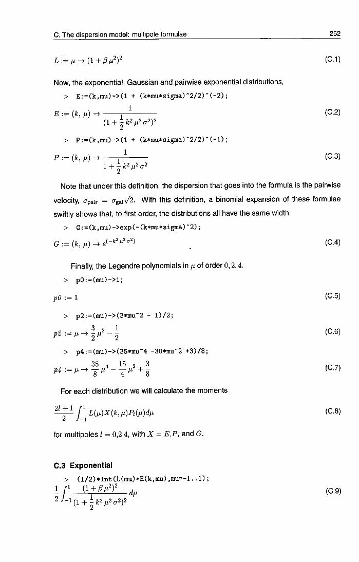
C. The d ispers ion mode l : mult ipole formulae 252
L : = M ^ ( 1 + / 3 ^ Y (C . I )
Now, the exponential, Gaussian and painwise exponential distributions,
> E : = ( k , m u ) - > ( 1 + ( k * m u * s i g m a ) " 2 / 2 ) " ( - 2 ) ;
E [k, /x) ~ (C .2)
(1 + - A ; V 2 ^ 2 P
> P : = ( k , m u ) - > ( 1 + ( k * m u * s i g m a ) " 2 / 2 ) * ( - l ) ;
P := {k, /i) ^ (C.3) 1 + ^k^lJi^a^
Note that under this definition, the dispersion that goes into the formula is the pairwise
velocity, cjpair = cTgaiv^. With this definition, a binomial expansion of these formulae
swiftly shows that, to first order, the distributions all have the same width.
> G : = ( k , m u ) - > e x p ( - ( k * m u * s i g m a ) " 2 ) ;
G:=(A; , Ai)-^e(-'=''^'<^') _ (C .4)
Finally, the Legendre polynomials in fi of order 0 , 2 , 4 .
> p O : = ( m u ) - > l ;
pO := 1 (C.5)
> p 2 : = ( m u ) - > ( 3 * m u * 2 - l ) / 2 ;
P S : = M ^ ^ M ' - ^ (C.6)
> p 4 : = ( m u ) - > ( 3 5 * r a u " 4 - 3 0 * m u " 2 + 3 ) / 8 ;
W : = / . - > f / - + ^ (C.7)
For each distribution we will calculate the moments
j\{n)X{k,,j.)Pi{ij)dii (C .8)
for multipoles / = 0,2,4, with X = E,P, and G.
C.3 Exponential > ( l / 2 ) * I n t ( L ( m u ) * E ( k , m u ) , m u = - l . . 1 ) ;
^l±iji^i, (C.9)

C. T h e d ispers ion mode l : mult ipole formulae 253
> ( l / 2 ) * i n t ( L ( m u ) * E ( k , m u ) , m u = - l . . 1 ) ;
( 2 4 ^ 2 ^ ^ 8 0 2 ^ 3 _^ 2 -t- 2 \ / 2 % 1 k^ a" - I - \ / 2 % 1 k^ - 24/^2 ^ /2 % 1
- 12 ^2 ^ % 1 ^2 2 _ 8 ^3 ^3 ^ 8 ^ % 1 ^2 ^2 ^ 4 ^ 2 % 1 k" a " ) /(2A;5 CT^
(2 + i t2^2))
% 1 : = a r c t a n ( J f c ( T ^ )
> ( 5 / 2 ) * I n t ( L ( m u ) * E ( k , m u ) * p 2 ( m u ) , m u = - l . . 1 ) ;
5 l ( l + / 3 ; . 2 ) 2 ( 3 2 _ 1 ^
1 / ( C I O )
> ( 5 / 2 ) * i n t ( L ( m u ) * E ( k , m u ) * p 2 ( m u ) , m u = - l . . 1 ) ;
I{-144 \ / 2 % 1 A;2 a2 - 80 v /2 % 1 A;" - f 144 /? (T^ + 56 ;5 - 104 /32 A;3
-t- 144/32 ^2 2 ^ J2/32 v ^ % l A;" a ' ' - 240^02 ^c r - 2 k'^ + 240/J^ ^ % 1
+ 4V2%lk^a^-V2%lk^a^-12k^a^ + l2V2%lk^a'^-4pV2%lk^a^) /{k^
(2 + A;2a2))
% 1 : = a r c t a n ( ^ A ; a \ / 2 )
> ( 9 / 2 ) * I n t ( L ( m u ) * E ( k , m u ) * p 4 ( i n u ) , m u = - l . . 1 ) ;
(C.11) 9 ^1 ( l + / 3 M T ( f + o / 1
(H -^ ib2 ; i 2^2)2
> ( 9 / 2 ) * i n t ( L ( m u ) * E ( k , m u ) * p 4 ( m u ) , m u = - l . . 1 ) ;
- - ^ ( - 1 8 3 2 ^ 2 ^5 5 ^ 952/3 A: ^ 1 5 2 0 v /2 % 1 A; + 2520 \ / 2 % 1 fc^ a " I D
- 16800 /? V2 % 1 A;2 2 - 2232 /? ^ 2 % 1 A; - 36 /3 \ / 2 % 1 A; a * - 9 % 1 k^°
+ 1 8 9 6 0 p ' ^ V 2 % l k^ a2 - 12720(5 k'^ + 108/^^ \ / 2 % 1 A;
- I -162 \ / 2 % 1 A ; V * -h 3816 0^ ^%\A;" a ' ' - 150400^ k^ - 2520 A; - 23520 /J^ a
- I - 16800 pk^a^- 18 A; - 1200 A; cr^ + 9 9 2 0 1 3 k ^ a ^ + 23520 \/2 % 1 ) / ( A ^ cr^
(2 + A:2a2))
% 1 : = a r c t a i i ( J A ; a \ / 2 )

C. T h e d ispers ion mode l : mult ipole formulae 254
C.4 Gaussian > ( l / 2 ) * I n t ( L ( m u ) * G ( k , m u ) * p O ( m u ) , m u = - l . . 1 ) ;
i | \ l + ^ / i 2 ) 2 e ( - ^ ^ ^ ^ - ^ ) d M (C.12)
> ( l / 2 ) * i n t ( L ( m u ) * G ( k , m u ) * p O ( m u ) , m u = - l . . 1 ) ;
il ^AFerf (A a) k' a' e^'' '^'^ - f3 k'a'+ ]-k'a'P V^e r f (A; a) e^'' <^')
4 8 '
> ( 5 / 2 ) * I n t ( L ( m u ) * G ( k , m u ) * p 2 ( m u ) , m u = - l . . 1 ) ;
\f_{l + P ^ ' ? e ^ - ' ' ^ ' ' ' ' ^ { \ l ^ ' - \ ) d t . (C.13)
> ( 5 / 2 ) * i n t ( L ( m u ) * G ( k , m u ) * p 2 ( m u ) , m u = - l . . 1 ) ;
5(_ ^ ^5 ^ 5 + 3 ^ ej.f ^ ) ^4 ^ 4 .2) _ 1 y^g^f ^ ) ^6 ^6 <r ) _ ^ ^ 5 _ 9 ^ ^3 ^ 3
+ I ^2 ^ 2 ^ ^ e r f (A; a) e^'^' < ') - ^ fc^ /? ^/^erf (A; a) e^'' "'^ _ i ^ 2 ^5 ^ 5 _ 3 ^ 2 ^3 ^3 8 4 z 2
_ 1 | ^ 2 ^ ^ + 45 ^ 2 ^ ^ ^ ^ ^ ^ ^ ( , . ,2) _ 3 ^ 2 ;^2 ^ 2 y ^ , ^ f a) e ' ^ <^ ))e(-'=^ ' ^) /(/=^ a^) 16 32 l b '
> ( 9 / 2 ) * I n t ( L ( m u ) * G ( k , m u ) * p 4 ( m u ) , m u = - l . . 1 ) ;
9
2
> ( 9 / 2 ) * i n t ( L ( m u ) * G ( k , m u ) * p 4 ( m u ) , m u = - l . . 1 ) ;
£ ( 1 + P,?f e(-'' / _ 1 ^ ^ 2 ^ ^ ) (C.14)
( - ^ Ac-* ^ ^ e r f ( A ; a) e^ ^ + A: /3 ^^erf(A; a) e ^
- ^ erf (A; a) k' e^^' + erf (A: a) k' a' e^>^' '^'^-9pk'a'
+ ^k^<^'p V ^ e r f (A; a) e^^' '^') + ^ V^e r f (fc a) k' a' e^^' -10^ a' ~—0^ k^ a'
+ ^ A; erf (A; a) e ^ - ^ _ 4725 ^ ^3 , 3
C.5 Pairwise exponential
> ( l / 2 ) * I n t ( L ( m u ) * P ( k , m u ) * p O ( m u ) , m u = - i . . 1 ) ;
l / ' J i l ^ r f . (C .15 )

C. T h e d ispers ion mode l : mult ipole formulae 255
> ( l / 2 ) * i n t ( L ( m u ) * P ( k , m u ) * p O ( m u ) , m u = - l . . 1 ) ;
1(2/3'^ k^ + 12pk^ - 1213'^ ka + 3V2arctan( J A;cr \ ^ ) A;" a ' '
- 1 2 / 3 \ / 2 a r c t a n ( ^ A; a V ^ ) A;2 cr2 + 12p'^ \ ^ a r c t a n ( ^ kaV2)) /{k^ a^)
> ( 5 / 2 ) * I n t ( L ( m u ) * P ( k , m u ) * p 2 ( m u ) , m u = - l . . 1 ) ;
U r-^ (C.16)
> ( 5 / 2 ) * i n t ( L ( m u ) * P ( k , i n u ) * p 2 ( m u ) , m u = - l . . 1 ) ;
^ (8 /32 A;^ cr^ -I- 360 /32 A; a - 15 V 2 % 1 A;^ + 90 A;^ - 90 ^ / 2 % 1 A;* a " 6
+ 60 /3 % 1 A;^ cr^ -I- 360 ;5 % 1 A;2 a'^ - 360 pk^a^- 60 p'^ V2%1 k^
-360fV2%l) /{k'^a^)
%1 := a r c t a n ( i A ; C T \ / 2 )
> ( 9 / 2 ) * I n t ( L ( m u ) * P ( k , m u ) * p 4 ( m u ) , m u = - l . . 1 ) ;
2 ^ - 1 1 + 1^2^2^2
> ( 9 / 2 ) * i n t ( L ( m u ) * P ( k , m u ) * p 4 ( m u ) , m u = - l . . 1 ) ;
^ ( - 4 2 0 k^ + 1680/3 A; - 110 A; + UOpk^ a^-36pV2 % 1 A: 8
- f 36 /32 7 2 % 1 A;* a ' ' -h 9 \ / 2 % 1 A;« - 1680 ^2 a + 1680 ^2 ^ % 1
- 1680 V 2 % 1 A;2 (T2 - f 420 % 1 A; - 440 /32 k^ + 720 /32 v /2 % 1 A;2
+ 180V2%lk^a^- 720l3V2%lk'^a'^) /{k^a^)
%1 := a r c t a n ( ^ A ; a v / 2 )
(C.17)

References
Abbreviations
MNRAS; Monthly Notices of the Royal Astronomical Society
ApJ; The Astrophysical Journal
ApJ Lett; The Astrophysical Journal Letters
ApJ Supp; The Astrophysical Journal Supplement
AJ; The Astronomical Journal
A&A; Astronomy & Astrophysics
A&A Supp; Astronomy & Astrophysics Supplement
ARA&A; Annual Review of Astronomy & Astrophysics
Ap&SS; Astrophysics and Space Science
References
ArpH. , 1999, A&A, 341, L5
Bagia J. S., 1998, MNRAS, 299, 417
Ballinger W. E., Heavens A. F, Taylor A. N., 1995, MNRAS, 276, L59
Ballinger W. E., Peacock J. A., Heavens A. F, 1996, MNRAS, 282, 877
Bardeen J., Bond J., Kaiser N., Szalay A., 1986, ApJ, 304,15
Barlow R. J., 1989, Statistics: a guide to the use of statistical methods in the physical
sciences, Manchester physics series. Wiley
Barrow J. D., Magueijo J., 1999, Physics Letters B, in press, astro-ph/9811072
Baugh C. M., 1996, MNRAS, 280, 267

References 257
Baugh C. M., Efstathiou G., 1993, MNRAS, 265,145
Baugh C. M., Efstathiou G., 1994, MNRAS, 267, 323
Baugh C. M., Gaztanaga E., Efstathiou G., 1995, MNRAS, 275,1049
Bean A. J., Ellis R. S., Shanks T, Efstathiou G., Peterson B. A., 1983, MNRAS, 205, 605
Benson A. J., Cole S., Baugh C. M., Frenk C. S., Lacey C. G., 1999, MNRAS
Bertin E., Dennefeld M., 1997, A&A, 317, 43
Bond J., Efstathiou G., 1991, Phys. Lett. B, 265, 245
Bond J. R., Kaiser N., Cole S., Efstathiou G., 1991, ApJ, 379, 440
Bouchet F. R., Colombi S., HIvon E., Juszklewicz R., 1995, A&A, 296, 575
Boulanger F., Perault M., 1988, ApJ, 330, 964
Bower R. G., Coles R, Frenk C. S., White S. D. M., 1993, ApJ, 405, 403
Bromley B. C , Warren M. S., Zurek W. H., 1997, ApJ, 475, 414
Burstein D., Heiles C , 1978, ApJ, 225, 40
Burstein D., Heiles C , 1982, AJ, 87,1165
Burstein D., McDonald L. H., 1975, AJ, 80,17
Canavezes A. et al., 1998, MNRAS, 297, 777
Carlberg R. G., Couchman H. M. R, Thomas R A., 1990, ApJ Lett, 352, L29
Carlberg R. G., Yee H. K. C , Ellingson E., 1997, ApJ, 478, 462
Carlberg R. G. et al., 1998, In Large Scale Structure in the Universe, Royal Society
Discussion Meeting, March 1998
Cen R., Ostriker J. R, 1992, ApJ, 399, 331
Cen R., Ostriker J. R, 1993, ApJ, 417, 415
Chaboyer B., Demarque R, Kernan R J., Krauss L. M., 1996, Science, 271, 957
Cheng E. S. et al., 1997, ApJ Lett, 488, L59
Cole S., 1997, MNRAS, 286, 38
Cole S., Fisher K. B., Weinberg D. H., 1994, MNRAS, 267, 785
Cole S., Fisher K. B., Weinberg D. H., 1995, MNRAS, 275, 515
Cole S., Weinberg D. H., Frenk C. S., Ratra B., 1997, MNRAS, 289, 37
Colless M., 1995, The 2df galaxy redshift survey,
http://msowww.anu.edu.aurheron/Colless/colless.html
Colless M., Ellis R. S., Taylor K., Hook R. N., 1990, MNRAS, 244, 408
Couchman H. M. R, 1991, ApJ, 368, 23
da Costa L. N. et al., 1994, ApJ, 424,1

References 258
da Costa L. N. et al., 1988, ApJ, 327, 544
da Costa L. N., Vogeley M. S., Geller M. J., Huchra J. R, Park C , 1994, ApJ Lett, 437, LI
Davis M., Efstathiou G., Frenk C. S., White S. D. M., 1985, ApJ, 292, 371
Davis M., Faber S. M., 1998, astro-ph/9810489. Preprint
Davis M., Peebles R J. E., 1983, ApJ, 267, 465
Dekel A., 1998, in Wide Field Surveys in Cosmology, 14th lAP meeting held May 1998,
Paris. Editions Frontieres., p. 47
Efstathiou G., Bond J. R., White S. D. M., 1992, MNRAS, 258,1
Efstathiou G., Davis M., White S. D. M., Frenk C. S., 1985, ApJS, 57, 241
Efstathiou G., Sutherland W. J., Maddox S. J., 1990, Nature, 348, 705
Eisenstein D. J., Hu W., 1998, ApJ, 496, 605
Eke V. R., Cole S., Frenk C. S., 1996, MNRAS, 282, 263
Eke V. R., Cole S., Frenk C. S., Henry J. R, 1998, MNRAS, 298,1145
Epchtein N. et al., 1994, Ap&SS, 217, 3
Faber S. M., 1973, ApJ, 179, 731
Fan Z. H., Bardeen J. M., 1994, American Astronomical Society Meeting, 184, 6206
Feldman H. A., Kaiser N., Peacock J. A., 1994, ApJ, 426,23
Ferreira R G., Magueijo J., Gorski K. M., 1998, ApJ Lett, 503, LI
Fisher K. B., 1992, Ph.D. thesis, AA (California Univ.)
Fisher K. B., 1995, ApJ, 448, 494
Fisher K. B., Davis M., Strauss M. A., Yahil A., Huchra J. R, 1994, MNRAS, 267, 927
Fisher K. B., Nusser A., 1996, MNRAS, 279, LI
Frenk C. S., Evrard A. E., White S. D. M., Summers R J., 1996, ApJ, 472, 460
Gardner J. P., Sharpies R. M., Frenk C. S., Carrasco B. E., 1997, ApJ Lett, 480, L99
Geller M. J., De Lapparent V., Kurtz M. J., 1984, ApJ Lett, 287, L55
Geller M. J., Huchra J. R, 1989, Science, 246, 897
Giovanelli R., Haynes M. R, 1991, ARA&A, 29, 499
Gorski K., 1988, ApJ, 332, L7
Governato R, Baugh C. M., Frenk C. S., Cole S., Lacey C. G., Quinn T, Stadel J., 1998,
Nature, 392, 359
Gregory S. A., Thompson L. A., 1978, ApJ, 222, 784
Groth E. J., Peebles R J. E., 1977, ApJ, 217, 385

References 259
Gunn J. E., Weinberg D. H., 1995, in proceedings of the 35th Herstmonceux workshop.
Cambridge University Press, Cambridge, astro-ph/9412080
Hamilton A. J. S., 1993, ApJ Letters, 406, 47
Hamilton A. J. S., 1997, astro-ph/9708102
Hamilton A. J. S., Kumar R, Lu E., Matthews A., 1991, ApJ Lett, 374, LI
Hancock S., Gutierrez C. M., Davies R. D., Lasenby A. N., Rocha G., Rebolo R., Watson
R. A., Tegmark M., 1997, MNRAS, 289, 505
Heavens A. F, Taylor A. N., 1995, MNRAS, 275, 483
Heavens A. F, Taylor A. N., 1997, MNRAS, 290,456
Heiles C , 1975, A&A Supp, 20, 37
Heiles C , 1976, ApJ, 204, 379
Henry J. R, Arnaud K. A., 1991, ApJ, 372, 410
Heydon-Dumbleton N. H., Collins C. A., Macgillivray H. T , 1989, MNRAS, 238, 379
Hilditch R. W., Hill G., Barnes J. V., 1976, MNRAS, 176,175
Hubble E., 1929, Proc N.A.S., 15,168
Huchra J. E. et al., 1992, in Center for Astrophysic Redshift catalog, 1992 version.
Huchra J. E., Davis M., Latham D., Tonry J., 1983, ApJS, 52, 89
Humason M. L , 1931, ApJ, 74, 35
Humason M. L , Mayall N. U., Bandage A. R., 1956, AJ, 61, 97
Jackson J. C , 1972, MNRAS, 156, IP
Jain B., Mo H. J., White S. D. M., 1995, MNRAS, 276, L25
Jenkins A. et al., 1998, ApJ, 499, 20
Jimenez R., Padoan R, 1998, ApJ, 498, 704
Jones L. R., Fong R., Shanks T, Ellis R. S., Peterson B. A., 1991, MNRAS, 249, 481
Kaiser N., 1987, MNRAS, 227,1
Kantor F. W., 1977, Information Mechanics. Wiley, New York
Kantor F W., 1999, International Journal of Theoretical Physics, accepted,
astro-ph/9812444
Katz N., Hernquist L., Weinberg D. H., 1992, ApJ Lett, 399, LI09
Kauffmann G., Nusser A., Steinmetz M., 1997, MNRAS, 286, 795
Kauffmann G., White S., Guiderdoni B., 1993, MNRAS, 264, 201
Kay S. T , Bower R. G., 1998, MNRAS, in press, astro-ph/9807240
Kirshner R. R, Oemler J., A., Schechter R L, 1978, AJ, 83,1549

References 260
Kirshner R. R, Oemler J., A., Schechter R L., Shectman S. A., 1981, ApJ Lett, 248, L57
Kogut A., Banday A. J., Bennett C. L., Gorski K. M., Hinshaw G., Smoot G. R, Wright
E. L , 1996, ApJ Lett, 464, L29
Kolb E. W., Turner M. S., 1990, The early universe. Addison-Wesley
Kristian J., Minkowski R., 1972, in Sandage A., Sandage M., Kristian J., ed, Galaxies in
the Universe. University of Chicago press
Lawrence C. R., Lange A. E., 1997, American Astronomical Society Meeting, 191, 4120
Lin H., Kirshner R. R, Shectman S. A., Landy S. D., Oemler A., Tucker D. L., Schechter
R L , 1996, ApJ, 471,617
Loveday J., Efstathiou G., MaddoxS. J., Peterson B. A., 1996, ApJ, 468,1
Loveday J., Efstathiou G., Peterson B. A., Maddox S. J., 1992a, ApJ Lett, 400, L43
Loveday J., Peterson B. A., Efstathiou G., Maddox S. J., 1992b, ApJ, 390, 338
LucyL. B., 1974, AJ, 79, 745
Maddox S. J., Efstathiou G., Sutherland W. J., 1996, MNRAS, 283,1227
Maddox S. J., Efstathiou G., Sutherland W. J., Loveday J., 1990a, MNRAS, 243, 692
Maddox S. J., Efstathiou G., Sutherland W. J., Loveday J., 1990b, MNRAS, 242, 43P
Mann R. G., Peacock J. A., Heavens A. F, 1998, MNRAS, 293, 209
Matsubara T., Suto Y, 1996, ApJ, 470,1
Meiksin A., White M., 1999, MNRAS, submitted, astro-ph/9812129
Melott A. L., Pellman T. E., Shandarin S. F, 1994, MNRAS, 269, 626
Metcalfe N., Shanks T , Fong R., Jones L. R., 1991, MNRAS, 249, 498
Mo H. J., Jing Y R, Borner G., 1997, MNRAS, 286, 979
Moore B., Frenk C. S., White S. D. M., 1993, MNRAS, 261, 827
Nakamura T. T , Matsubara T , Suto Y, 1998, ApJ, 494, 13
Netterfield C. B., Devlin M. J., Jarolik N., Page L., Wollack E. J., 1997, ApJ, 474, 47
Nichol R. C , Collins C. A., 1993, MNRAS, 265, 867
Pahre M. A., Djorgovski S. G., De Carvalho R. R., 1996, ApJ Lett, 456, L79
Park C , Vogeley M. S., Geller M. J., Huchra J. R, 1994, ApJ, 431, 569
Peacock J. A., Dodds S. J., 1994, MNRAS, 267,1020
Peacock J. A., Dodds S. J., 1996, MNRAS, 280, LI 9
Peebles P. J. E., 1980, The large-scale structure of the universe. Princeton University
Press, Princeton, N.J.
Peebles R J. E., 1981, ApJ, 248, 885
References 261
Peebles R J. E., 1993, Principles of Physical Cosmology. Princeton University Press, Princeton
Perlmutter S. et al., 1999, ApJ, in press, astro-ph/9812133
Philips L. A., Turner E. L., 1998, ApJ, submitted, astro-ph/9802352
Pound R. v., Rebka G. A., 1959, Phys. Rev. Lett., 3, 439
Press W. H., Schechter R, 1974, ApJ, 187, 425
Press W. H., Teukolsky S. A., Vetterling W. T, Flannery B. R, 1992, Numerical Recipes
in FORTRAN, 2nd edition. Cambridge University Press, Cambridge
Ratcliffe A., Shanks T , Broadbent A., Parker Q. A., Watson F G., Gates A. R, Fong R.,
Collins C. A., 1996, MNRAS, 281, L47
Ratcliffe A., Shanks T , Parker Q. A., Fong R., 1998b, MNRAS, 293,197
Ratcliffe A., Shanks T , Parker Q. A., Fong R., 1998a, MNRAS, 296,191
Renzini A. et al., 1996, ApJ Lett, 465, L23
Rowan-Robinson M. etal . , 1990, MNRAS, 247, 1
Rugers M., Hogan C. J., 1996, ApJ Lett, 459, LI
Salaris M., Degl'Innocenti S., Weiss A., 1997, ApJ, 484, 986
Sandage A., Tammann G., 1987, in Carnegie Institution of Washington Publication,
Washington: Carnegie Institution, 1987, 2nd ed.
Santiago B. X., Strauss M. A., Lahav O., Davis M., Dressier A., Huchra J. R, 1995, ApJ,
446, 457
Sargent W. W., Turner E. L., 1977, ApJ, 212, L3
Saunders W. et al., 1994, in Proceedings of the 35th Herstmonceux workshop.
Cambridge University Press, Cambridge
Schechter R, 1976, ApJ, 203, 297
Scherrer R. J., Weinberg D. H., 1998, ApJ, 504, 607
Schlegel D. J., Finkbeiner D. P., Davis M., 1998, in Wide Field Surveys in Cosmology,
eds. S. Colombi and Y. Mellier
Schlegel D. J., Finkbeiner D. R, Davis M., 1998, ApJ, 500, 525
Schmidt B. R et al., 1998, ApJ, 507,46
Seljak U., Zaidarriaga M., 1996, ApJ, 469, 437
Shane C. D., Wirtanen C. A., 1967, Pub. Lick Obs., 22, 1
Shectman S. A., Landy S. D., Oemler A., Tucker D. L., Lin H., Kirshner R. R, Schechter
R L , 1996, ApJ, 470, 172

References 262
Smoot G. F et al., 1992, ApJ Lett, 396, LI
Smoot G. F, Gorenstein M. V., Muller R. A., 1977, Physical Review Letters, 39, 898
Soifer B. T , Sanders D. B., Madore B. R, NeugebauerG., Danielson G. E., Elias J. H.,
Lonsdale C. J., Rice W. L., 1987, ApJ, 320, 238
Stark A. A., Gammie C. F, Wilson R. W., Bally J., Linke R. A., Heiles C , Hunwitz M.,
1992, ApJ Supp, 79, 77
Steigman G., 1976, ARA&A, 14, 339
Strauss M. A., Davis M., Yahil A., Huchra J. R, 1990, ApJ, 361, 49
Strauss M. A., Huchra J. R, Davis M., Yahil A., Fisher K. B., Tonry J., 1992, ApJ Supp,
83, 29
Strauss M. A., Willick J. A., 1996, Physics Reports, 261, 271
Stuart A., 1987, Kendall's Advanced theory of statistics, 5th ed. Vol.1: Distribution
theory. Charles Griffin, London
Sugiyama N., 1995, ApJ Supp, 100, 281
Summers R J., Davis M., Evrard A. E., 1995, ApJ, 454,1
Sunyaev R. A., Zel'dovich Y. B., 1972, Comm. Astrophys. Space Phys., 4,173
Sylos Labini F, Montuori M., 1998, A&A, 331, 809
Tadros H. et al., 1998, in Large Scale Structure: Tracks and Traces. Proceedings of the
12th Potsdam Cosmology Workshop, September 1997. Eds. V. Mueller, S.
Gottloeber, J.R Muecket, J. Wambsganss. World Scientific, p. 221
Tadros H., Efstathiou G., 1995, MNRAS, 276, 45
Tanvir N., Shanks T , Ferguson H., Robinson D., 1995, Nature, 377, 27
Taylor A. N., Hamilton A. J. S., 1996, MNRAS, 282, 767
Tegmark M., 1996, in Dark matter in the universe: Proc. Enrico Fermi, Course CXXXII,
astro-ph/9511148
Tormen G., Bertschinger E., 1996, ApJ, 472,14
Trumpler R. J., 1930, Lick Observatory Bulletin, 420,154
Tully R. B., Fisher J. R., 1987, in Cambridge: University Press, 1987
Tytler D., Fan X.-M., Buries S., 1996, Nature, 381, 207
Walker T R, Steigman G., Kang H.-S., Schramm D. M., Olive K. A., 1991, ApJ, 376, 51
Wasserburg G. J., Papanastassiou D. A., Tera F, Huneke J. C , 1977, Royal Society of
London Philosophical Transactions Series, 285, 7

References 263
Watson G. N., 1922, A treatise on the theory of Bessel functions. Cambridge University Press
Weinberg D. H., Cole S., 1992, MNRAS, 259, 652
Wheelock S. L. et a!., 1994, IRAS sky survey atlas: Explanatory supplement. JPL
publication 94-11
White M., Bunn E., 1996, ApJ, 460,1071
White M., Bunn E. F, 1995, ApJ, 450, 477
White S. D. M., 1996, in Schaeffer R., ed, Cosmology and large scale structure : Les
Houches, session LX, 1-28 August 1993. Elsevier Science, Amsterdam,
astro-ph/9410043
White S. D. M., Efstathiou G., Frenk C. S., 1993, IVINRAS, 262,1023
White S. D. M., Frenk C. S., Davis M., Efstathiou G., 1987, ApJ, 313, 505
Yee H. K. C, Ellingson E., Carlberg R. G., 1996, ApJS, 102, 269
Zaroubi S., Hoffman Y, 1996, ApJ, 462, 25
ZeI'dovich Y B., 1970, A&A, 5, 84
ZeI'dovich Y B., 1972, MNRAS, 160, IP
Zucca E. et al., 1996, Astrophysics Letters and Communications, 33, 99
Zucca E. et al., 1997, A&A, 326, 477