Durham E-Theses Decentralised Optimisation and Control in ...
155
• • •
Transcript of Durham E-Theses Decentralised Optimisation and Control in ...
Durham E-Theses
Decentralised Optimisation and Control in Electrical
Power Systems
LOUKARAKIS, EMMANOUIL
How to cite:
LOUKARAKIS, EMMANOUIL (2016) Decentralised Optimisation and Control in Electrical Power
Systems, Durham theses, Durham University. Available at Durham E-Theses Online:http://etheses.dur.ac.uk/11601/
Use policy
The full-text may be used and/or reproduced, and given to third parties in any format or medium, without prior permission orcharge, for personal research or study, educational, or not-for-pro�t purposes provided that:
• a full bibliographic reference is made to the original source
• a link is made to the metadata record in Durham E-Theses
• the full-text is not changed in any way
The full-text must not be sold in any format or medium without the formal permission of the copyright holders.
Please consult the full Durham E-Theses policy for further details.

Academic Support O�ce, Durham University, University O�ce, Old Elvet, Durham DH1 3HPe-mail: [email protected] Tel: +44 0191 334 6107
http://etheses.dur.ac.uk
2
Decentralised Optimisation & Control
in Electrical Power Systems
by
Emmanouil Loukarakis
A dissertation submitted for the degree of
Doctor of Philosophy in Engineering
School of Engineering & Computing Sciences
Durham University
2015


i
Abstract
Emerging smart-grid-enabling technologies will allow an unprecedented degree of observability
and control at all levels in a power system. Combined with flexible demand devices (e.g. electric
vehicles or various household appliances), increased distributed generation, and the potential
development of small scale distributed storage, they could allow procuring energy at minimum
cost and environmental impact. That however presupposes real-time coordination of demand of
individual households and industries down at the distribution level, with generation and
renewables at the transmission level. In turn this implies the need to solve energy management
problems of a much larger scale compared to the one we currently solve today. This of course
raises significant computational and communications challenges.
The need for an answer to these problems is reflected in today’s power systems literature where
a significant number of papers cover subjects such as generation and/or demand management at
both transmission and/or distribution, electric vehicle charging, voltage control devices setting,
etc. The methods used are centralized or decentralized, handling continuous and/or discrete
controls, approximate or exact, and incorporate a wide range of problem formulations. All these
papers tackle aspects of the same problem, i.e. the close to real-time determination of operating
set-points for all controllable devices available in a power system. Yet, a consensus regarding the
associated formulation and time-scale of application has not been reached. Of course, given the
large scale of the problem, decentralization is unavoidably part of the solution. In this work we
explore the existing and developing trends in energy management and place them into perspective
through a complete framework that allows optimizing energy usage at all levels in a power
system.

iii
Contents
1 Introduction & Scope ......................................................................................................................... 1
1.1 Point of Reference ........................................................................................................................ 1
1.2 Identifying the Problem ................................................................................................................ 2
1.3 Distributed & Decentralized Solutions ........................................................................................... 4
1.4 Avoiding Commitment ................................................................................................................. 5
1.4.1 Aggregator Bidding ............................................................................................................... 6
1.4.2 Unit Commitment Formulations ............................................................................................ 7
1.5 Closer to Real-Time ...................................................................................................................... 8
1.6 Contributions & Structure ............................................................................................................. 9
2 Optimal Power Flow ..........................................................................................................................13
2.1 Problem Perspective ....................................................................................................................13
2.2 Modelling Power Systems Devices ...............................................................................................13
2.2.1 Sequences Reference Frame ................................................................................................14
2.2.2 Overhead Lines Impedance ..................................................................................................15
2.2.3 Transformers .......................................................................................................................16
2.2.4 Phase Configurations & Generic Device Model .....................................................................18
2.3 Optimal Power Flow Standard Formulation .................................................................................19
2.4 Branch Flow Model (Radial Networks Only) .................................................................................21
2.5 DC Load Flow (Transmission Only) ...............................................................................................22
2.6 Convex Relaxations .....................................................................................................................23
2.6.1 Semi Definite Programming .................................................................................................23
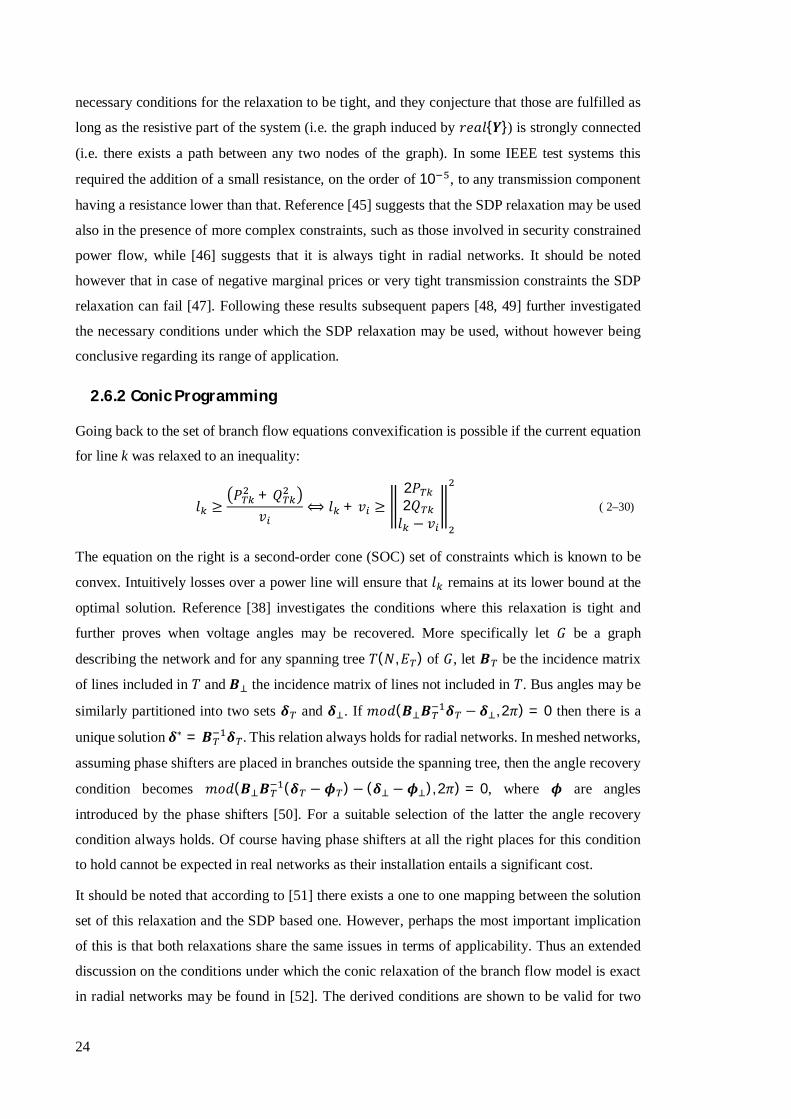
2.6.2 Conic Programming..............................................................................................................24
2.7 Unbalanced Optimal Power Flow Generic Formulation ................................................................25
2.8 Current Injection Approximations (Distribution Only) ...................................................................28
2.8.1 Current Approximation Approach for Unbalanced Networks ................................................28
2.9 Mathematical Programming for OPF ...........................................................................................31
2.9.1 Penalty Methods..................................................................................................................32
2.9.2 Sequential Programming Methods .......................................................................................33
iv
2.9.3 Interior Point Methods (IPM) ............................................................................................... 34
2.9.4 Trust-Region Methods ......................................................................................................... 36
2.9.5 Implementation Considerations........................................................................................... 37
2.10 Conclusions & Further Questions ............................................................................................... 40
3 Decentralized Optimal Power Flow ................................................................................................... 43
3.1 Problem Statement..................................................................................................................... 43
3.2 Decomposition Structure ............................................................................................................ 43
3.2.1 Distributed Optimization Underlying Principle ..................................................................... 44
3.2.2 Decomposition Schemes ..................................................................................................... 44
3.2.3 Spectral Partitioning ............................................................................................................ 46
3.2.4 k-Means Clustering.............................................................................................................. 47
3.3 Decomposition Methods ............................................................................................................. 47
3.3.1 Dantzig-Wolfe Decomposition ............................................................................................. 47
3.3.2 Benders Decomposition ...................................................................................................... 49
3.3.3 Lagrangian Relaxation (LR)................................................................................................... 49
3.3.4 Alternating Direction Method of Multipliers (ADMM) .......................................................... 54
3.3.5 Predictor Corrector Proximal Multipliers Method (PCPM) .................................................... 56
3.3.6 Adaptive Proximal Decomposition Method (APDM) ............................................................. 57
3.3.7 Auxiliary Problem Principle (APP)......................................................................................... 58
3.3.8 Optimality Condition Decomposition (OCD) ......................................................................... 59
3.3.9 Other Approaches ............................................................................................................... 61
3.4 Results and Discussion ................................................................................................................ 62
3.4.1 Decomposition Example ...................................................................................................... 63
3.4.2 Parameter Selection ............................................................................................................ 64
3.4.3 Effects of System Size .......................................................................................................... 66
3.4.4 Value of Aggregation ........................................................................................................... 67
3.4.5 Convergence Considerations ............................................................................................... 70
3.5 Conclusions & Further Questions................................................................................................. 70
4 Extended Economic Dispatch ............................................................................................................ 73
4.1 Extended Economic Dispatch ...................................................................................................... 73
4.1.1 Network Constraints............................................................................................................ 75
4.1.2 Generation Constraints ....................................................................................................... 75
4.1.3 Demand Constraints ............................................................................................................ 75
4.1.4 Coupling Constraints ........................................................................................................... 77
v
4.2 Economic Dispatch Simplifications ...............................................................................................78
4.2.1 Market Aggregator Structure ...............................................................................................79
4.2.2 Decentralized Solution .........................................................................................................80
4.2.3 Microgrid Operator Subproblems .........................................................................................81
4.2.4 Microgrid Level Aggregation ................................................................................................82
4.2.5 An Indicative Example ..........................................................................................................84
4.3 Results and Discussion ................................................................................................................86
4.3.1 Base Test Case .....................................................................................................................86
4.3.2 Time-wise Scalability ............................................................................................................88
4.3.3 Network Scalability & Implementation Challenges................................................................89
4.3.4 Coordination ........................................................................................................................90
4.4 Conclusions & Further Questions .................................................................................................90
5 Microgrid Dispatch ............................................................................................................................93
5.1 Problem Perspective ....................................................................................................................93
5.2 Microgrid Controls ......................................................................................................................93
5.2.1 Pure Control ........................................................................................................................94
5.2.2 Centralized Energy Management – Network Unconstrained .................................................95
5.2.3 Centralized Energy Management – Network Constrained .....................................................97
5.2.4 Decentralized Perspective ....................................................................................................99
5.2.5 Concluding Remarks .......................................................................................................... 102
5.3 Utility Functions for Demand ..................................................................................................... 103
5.4 Problem Formulation ................................................................................................................ 104
5.5 Solving for the Continuous Controls ........................................................................................... 106
5.6 Integer Programming for OPF ................................................................................................... 109
5.6.1 Branch & Bound (BB) ......................................................................................................... 109
5.6.2 Cutting Planes .................................................................................................................... 111
5.6.3 Feasibility Heuristics .......................................................................................................... 111
5.6.4 Improvement Heuristics ..................................................................................................... 113
5.6.5 Other Approaches .............................................................................................................. 114
5.6.6 Modified Penalty-Based Method ........................................................................................ 115
5.7 Conclusions & Further Questions ............................................................................................... 116
6 Conclusions ..................................................................................................................................... 119
6.1 A Brief Summary ....................................................................................................................... 119

vi
6.2 Further Improvements & Extensions ......................................................................................... 120
7 References ...................................................................................................................................... 123
vii
Abbreviations & Mathematical Conventions
The following table summarizes abbreviations commonly used throughout the text, along
with the page where they are first explained:
DSO Distribution System Operator 41
ED Economic Dispatch 1
EV Electric Vehicle 2
LR Lagrangian Relaxation 45
MD Microgrid Dispatch 84
MO Microgrid Operator 41
OPF Optimal Power Flow 13
TSO Transmission System Operator 40
UC Unit Commitment 1
Furthermore, the following conventions apply in all mathematical equations (the variable
name ‘z’ is used as an example):
퐳 Bold font indicates a vector or matrix.
푧 Italics indicate a scalar.
퐳( , ) Indicates element (푥,푦) of matrix 퐳
퐳 Transpose of matrix 퐳
푧{ } Indicates a scalar (could also be a matrix or a function) associated with element x.
‖퐳‖ Indicates the squared Euclidean norm: for a 푛푥1 vector that is ∑ 퐳( )∈[ , ]
푑푖푎푔{퐳} Indicates a diagonal matrix whose diagonal elements are the elements of vector 퐳.
Σ(퐳) Indicates the sum of all elements of vector 퐳.


ix
Statement of Copyright
The copyright of this thesis rests with the author. No quotation from it should be published
without the author’s prior written consent and information derived from it should be
acknowledged.


xi
Acknowledgements
Good people make a good university and in that respect I feel that Durham is one of the best. This
is something that definitely helped make the bad aspects of a PhD more bearable, and the good
even better.
I would like to thank both my supervisors Janusz Bialek and Chris Dent for their support and
advice. Far beyond their help in academic matters, they made me feel welcome in Durham and
exposed me to numerous opportunities which helped my professional development. For that I am
particularly grateful. Of course I won’t forget the numerous dinners, and most importantly one on
Christmas ’13. It was definitely one of the best I had in UK, but to some extent remains a source
of disappointment, as I have consistently failed to reproduce that apple-crumble.
I would also like to thank friends and colleagues in my office who in their different ways made
my experience in Durham unique and memorable: Sean Norris, Mustafa Elsherif, Peter Wyllie,
Hongbo Shao, Donatella Zappala, Meng Xu, Terry Ho, Amy Wilson and Chiara Bordin.
I am also particularly grateful to Varvara Alimisi, as well as Ivan Castro and Cristina Gallego for
being patient with me these past three years and the many great times we had together. Thanks to
them life in UK has been much, much better.
Finally, I would especially like to thank my family for supporting and encouraging me throughout
this endeavour. Without them this would not have been possible.


xiii
List of Publications
Journal papers
[1] E. Loukarakis, C. Dent, J. Bialek, “Decentralized Multi-Period Economic Dispatch for Real-Time Flexible Demand Management,” IEEE Transactions Power Systems, *in press*
[2] E. Loukarakis, J. Bialek, C. Dent, “Investigation of Maximum Possible OPF Problem Decomposition Degree for Decentralized Energy Markets,” IEEE Transactions Power Systems, vol. 30, no. 5, pp. 2566-2578, 2015
Conference papers
[3] E. Loukarakis, J. Bialek, C. Dent, “A General Framework for Decentralized Trading in Electricity Markets,” IREP Bulk Power System Dynamics and Control Symposium, Rethymnon, Greece, 25-30 August 2013
[4] E. Loukarakis, C. Dent, “Distribution System Optimization for Real-Time Generation and Flexible Demand Management,” accepted in Power Systems Computation Conference, Genoa, Italy, 19-24 June 2016
Under review
[5] E. Loukarakis, C. Dent, “Decentralized Optimization & Control in Electrical Power Systems,” invited book chapter submission in Smarter Energy: From Smart Metering to the Smart Grid, IET

1
1 Introduction & Scope
The advent of smart grids along with the future need for managing efficiently a large number of flexible devices at the end-user level, has led to an increased interest in energy management applications in power systems. This in turn brought attention to decentralized methods for solving the potential problems associated with: 1) the significant computational and communications burden implied for centralized solutions; and 2) certain social aspects related to privacy of information and allowing energy usage decisions to remain with the end-user. However, the actual practical necessity and scope of application of decentralized approaches in power systems energy management remains quite obscure. In this chapter we set our general perspective on the subject and provide an overview of relevant problems and questions.
1.1 Point of Reference
Electrical power systems are operated today in a highly efficient manner using a largely
centralized structure. The latter consists of three basic successive mechanisms [1, 2] which control
the power system state at any point in time:
Unit Commitment (UC): a centralized mixed-integer optimization problem, covering a time
period of several hours, which determines the operating status of large conventional generators.
This is typically solved up to a day ahead of real-time, to account for the fact that large generators
may require several hours to start-up or shut-down [1, 3]. It should be noted however that
different versions of this problem may be solved closer to real-time for the specific purpose of
scheduling smaller fast-start generators.
Economic Dispatch (ED): a centralized non-linear and non-convex optimization problem,
covering a short period in time [4]. While in practice there may be a number of discrete devices
involved (e.g. capacitor banks or transformers), ED is commonly assumed in research literature
to involve only continuous constraints and controls [5]. It is solved several minutes ahead of
real-time and its purpose is determining the operating points of all controllable devices in the
system. Within this work we assume ED in its basic form to be a single time-step optimisation
problem, which includes transmission level network constraints.
Fast local controls: these involve the controllers of individual devices acting instantly based
on local signals of frequency or voltage. Their set-points and operation mode would typically be
determined through the ED mechanism. This could be considered as a decentralized control
scheme which unavoidably has to remain so, as the quickly evolving system dynamics do not

2
allow time for any coordination between individual devices. Note that some coordination is still
achieved through appropriate off-line tuning of device controller parameters.
Overall the above structure strikes a good balance between management of uncertainty and
individual problems solution speed and is supported by an appropriate market framework [6, 7].
UC and ED are the energy management mechanisms which try to achieve optimal (in terms of
economic efficiency and reliability) operation, while the fast local controls are there to ensure
system stability. This work focuses on the technical / engineering aspects of optimal energy
management problems, rather than issues related with fast controls and stability or the design of
the associated markets. Given that the above structure has been performing quite well for several
decades now, our starting question is whether or not, any change to it, or any push towards
decentralized approaches is at all necessary.
1.2 Identifying the Problem
The answer to the question above may become clear through a simple comparison between the
power system’s structure at present and its expected structure in the future. The changes are
evident on Fig.1-1. The centralized solution of relevant optimization problems in UC and ED is
still an active research area and there is no apparent consensus regarding their exact formulation
[3, 5]. In any case however, both UC and ED are about optimizing the operation of a mix of large-
scale conventional and renewable generation, subject to transmission network constraints, given
aggregate demand estimates at the transmission node level. As such the distribution networks or
individual end-user devices have never been considered in detail. This was a reasonable approach
given that end-users have been largely inflexible in their energy requirements, and as a
consequence, distribution networks were built to cover any foreseeable amount of demand. As a
result, their constraints in terms of energy management could simply be ignored. However, recent
trends in power system literature envision a high number of flexible demand devices – e.g. electric
vehicles (EVs) [8], small-scale storage [9], or simply controllable versions of today's appliances
[10] – in the near future.
The most dominant characteristic of flexible devices in terms of energy management is their time-
linking characteristics, i.e. instead of meeting a power requirement at a given instance of time (as
with today’s inflexible demand), energy requirements have to be met over a period of time. In
addition, most of these devices will be connected at the distribution level. These considerations
raise three basic issues which are not fully addressed through current energy management
mechanisms:
1. Demand coordination over time: Towards achieving efficient operation the use of these
flexible devices at the distribution level has to be coordinated with generation at the transmission
level, e.g. shift demand to hours when energy is cheap (either due to the fact that demand was
3
in the first place low, or due to increased renewable energy availability). However, this is not
covered by today’s formulations, where ED has at most a very limited look-ahead period in time
[4]. At the same time UC, which does optimize over long periods of time, is typically solved far
in advance and might not fully allow micromanaging individual devices.
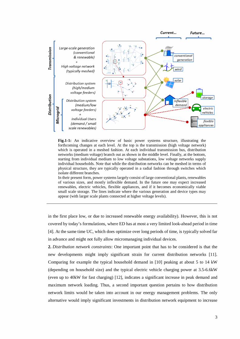
2. Distribution network constraints: One important point that has to be considered is that the
new developments might imply significant strain for current distribution networks [11].
Comparing for example the typical household demand in [10] peaking at about 5 to 14 kW
(depending on household size) and the typical electric vehicle charging power at 3.5-6.6kW
(even up to 40kW for fast charging) [12], indicates a significant increase in peak demand and
maximum network loading. Thus, a second important question pertains to how distribution
network limits would be taken into account in our energy management problems. The only
alternative would imply significant investments in distribution network equipment to increase
Fig.1-1: An indicative overview of basic power systems structure, illustrating the forthcoming changes at each level. At the top is the transmission (high voltage network) which is operated in a meshed fashion. At each individual transmission bus, distribution networks (medium voltage) branch out as shown in the middle level. Finally, at the bottom, starting from individual medium to low voltage substations, low voltage networks supply individual households. Note that while the distribution networks can be meshed in terms of physical structure, they are typically operated in a radial fashion through switches which isolate different branches. In their present form, power systems largely consist of large conventional plants, renewables of various sizes, and mostly inflexible demand. In the future one may expect increased renewables, electric vehicles, flexible appliances, and if it becomes economically viable small scale storage. The lines indicate where the various generation and device types may appear (with larger scale plants connected at higher voltage levels).

4
capacity. This again is something that traditionally has never been considered in either UC or
ED.
3. Controls assignment: One further evident question is when would a system operator assign
and adjust set-points or control modes to these new flexible devices. The nature of the control
or market signals that would be exchanged between them would also need to be clarified.
Without question, the basic energy management structure (presented in the previous section)
should evolve to account for these three issues. Only then would procurement of energy at the
minimum possible cost and environmental impact be possible. As such a change in the way UC
and ED problems are formulated and solved is unavoidable. Of course the most straightforward
solution would be to simply extend their formulations to include the requirements and limitations
of each individual device and network component. This however implies optimization problems
of a particularly large scale and three new issues would come to replace the ones solved, i.e.:
1. Tractability: these new problems might not be tractable through centralized methods, i.e. their
solution time may not be fast enough for the result to be of use for power system operations.
2. Communications: a centralized solution would require one operator communicating every few
seconds with millions of devices. It is uncertain whether a sufficiently fast and reliable solution
in terms of communications infrastructure is possible at a reasonable cost.
3. Privacy: while this is a rather subjective issue, sending a full schedule of one’s use of energy
and private activities, might be a problem for some individuals. The same is true with respect to
passing full control of the devices (e.g. an electric vehicle) one owns to one central operator.
These three points indicate the need for highly parallelizable and potentially decentralized
solution methods.
1.3 Distributed & Decentralized Solutions
When it comes to optimisation problem tractability – or in other words solution speed – there are
three possibilities for improvements: simplifying the problem, improving the solver, or
parallelizing the necessary computations [13]. The latter is something to be pursued on several
levels, e.g. the parallel execution of basic numerical operations in a processor (a core part of
modern computing systems), or the parallel solution of algebraic problems within the solver by
exploiting the structure of the associated mathematical method, or the parallel solution of parts of
the original problem by exploiting its structure. This latter higher level parallelization of the
problem solution is of interest in this work. It involves breaking apart the original problem into a
set of smaller subproblems and coordinating iteratively their solution through an appropriate
mathematical decomposition approach. The latter achieves this coordination in a way that is
mathematically proven to converge to the optimum of the original problem (global if the problem
is convex, possibly local if the problem is non-convex). Depending on how the coordination of
5
the subproblems is achieved the solution may be centralized or decentralized. In the following we
refer to problem solutions as:
distributed: a solution approach which rather than handling the whole problem at once,
decomposes it into smaller ones, and iteratively coordinates their solution to convergence;
centralized: a solution which is not distributed, or even if it is and subproblems are solved in
a distributed manner (e.g. in separate computing systems), coordination is achieved via
communication with one central controller;
decentralized: a distributed solution where there is no need for a central controller and
coordination is achieved through the communication between individual subproblems.
One further distinction could be made between synchronous and asynchronous methods.
synchronous: a distributed solution which requires that subproblem updates wait at specific
points for the arrival of certain data;
asynchronous: a distributed solution which performs subproblem updates and transmits
relevant information as soon as changes to subproblem parameters are registered. These methods
require a more rigorous assessment of their convergence properties.
Independently of whether or not a solution approach is decentralized, a distributed method should
in general be able to cope equally well with tractability problems. However, as will be discussed
in the following chapters, fully decentralized solutions may have reduced communication
infrastructure requirements, and depending on the transmitted information type, they may also
alleviate any privacy issues. Note that decentralized solutions are applicable in continuous
optimisation problems. For mixed integer problems, while distributed solutions are possible, some
sort of centralized control is typically necessary to reach a good quality solution.
1.4 Avoiding Commitment
In contrast to ED and its limited look-ahead period, UC could readily accommodate flexible
demand characteristics (e.g. scheduling an electric vehicle or storage unit over time) given its
typical multi-period formulation. However, one associated difficulty is that UC is characterized
by significant uncertainty. It is also a fact that UC is already a challenging mixed integer problem
when the objective is to schedule a few (relative to the number of small-scale flexible devices)
slow-to-start generators. Incorporating the constraints of individual devices or attempting to
include the details of distribution networks, would not only make the problem extremely large,
but it would also probably be of little practical value. This is due to the fact that it is unlikely that
demand at the end-user level could be reliably forecasted. This in turn implies that any control
decisions made for devices at the distribution level are also unlikely to be actually used, as they
would have to be validated and possibly changed closer to real-time. Consequently, aggregate
6
demand models appear to be a better option: e.g. trying to determine a schedule at hour 10 of the
following day of an EV with 0.5 probability of being connected might not be very meaningful,
whereas trying to schedule the aggregate consumption of a 100 such EVs (due to the much smaller
associated uncertainty) is more likely to give an answer of practical value. This conclusion is in
agreement with approaches published in recent relevant literature (e.g. [14, 15, 16]) which in
essence attempt to do the same thing, i.e. build appropriate reduced-order models for a collection
of flexible devices (most commonly EVs). The latter are assumed to be managed by a single
entity, the aggregator.
Overall, given the involved uncertainty, individual devices and distribution networks may not be
meaningfully optimized in the UC time-frame and full coordination to the individual device level
is not possible. Nevertheless, UC can definitely enable a certain degree of demand coordination
over time with generation, through the use of aggregate models. In addition, as will become clear
in the following, UC (currently being the only real-world optimization problem coordinating
devices over time in power systems) can provide some insight into uncertainty management and
model reduction approaches for large scale problems. In the following we briefly review how
device flexibility is managed within this particular problem.
1.4.1 Aggregator Bidding
In cases where the aggregators are participating as independent entities in the market, managing
on their own the uncertainty to which they are exposed, a reduced-order model is essentially built
through the process of constructing energy bids (i.e. roughly speaking prices vs. power curves).
For example, in [17] a simplified approach is presented for constructing bids for an EV
aggregator. Given that the relevant optimization problem when considering each individual
electric vehicle for all possible future scenarios would be intractable, the vehicles are grouped in
three basic categories, based on their expected way of charging (e.g. EVs charging on one of three
pre-agreed periods). The aggregator builds a forecast for each category and solves an optimization
problem that attempts to minimize costs and expected deviation penalties (i.e. differences of
power dispatched in ED compared to power initially scheduled in UC). A similar approach of
grouping vehicles, this time based on similarities in their usage patterns, is proposed in [18] where
the aggregator participation in a day-ahead market (including regulation services) is taken into
account through a linear programming formulation. Monte-Carlo simulation is used to generate
scenarios for electric vehicles and management of uncertainty is done through a point-estimate
method.
A scenario based approach is also used in [19], but without any sort of scenario reduction. The
aggregator simply generates a given number of scenarios by sampling distributions for all EV
parameters (e.g. connection time and state of charge) and given forecasts for the energy prices
7
solves a two-stage optimization problem. Detailed battery charging characteristics are considered,
i.e. a dependency between maximum power and state of charge (assuming Li-Ion batteries), and
represented through additional linear constraints. However, it is unclear what improvement this
offers compared to simpler approaches. Note that optimization control variables are associated
with each scenario and each electric vehicle scheduling realization, thus resulting in a particularly
large problem.
Reference [16] proposes a deterministic multi-period discrete optimization model for EV
charging which is solved via dynamic programming. It also considers vehicle participation in
regulation markets and provides some insight into the economic viability of electric vehicles. The
scheduling and dispatch problems for EVs are formulated and solved separately, with the
aggregator trying to buffer the errors in terms of EVs behaviour during the dispatch process. In
[20] the aggregator submits an inflexible energy bid as well as a flexible energy bid for regulation
services. The bid is derived based on a stochastic dynamic programming approximation. It is
assumed that the aggregator has knowledge of the resulting probability distribution of energy and
regulation prices. EVs are grouped based on their departure times and a penalty is applied if a
vehicle departs without being charged at the desired level.
Finally, [21] studies the participation of EVs combined with storage in forward and balancing
energy markets including the provision of regulation. Each vehicle is assumed to provide
information regarding its energy requirements and charging time as soon as it is connected. Point-
estimates are used for uncertain quantities and a generic discrete model is used for EVs. The
resulting mixed integer programming problem is solved using a heuristic based on a linear
programming relaxation.
The papers referenced above are indicative of the research currently being carried out in terms of
managing flexible demand within UC, and apparently there is an abundance of methods to do it.
At this point it is possible to make two interesting observations. The first is that managing
uncertainty locally at the aggregator level (through the submission of aggregate bids or other
aggregate models) appears to be a common enough and sensible approach which can greatly
simplify the UC problem’s solution. The second relates to the simple fact that, as may be expected,
the aggregation process presupposes an additional dispatch step for individual devices closer to
real-time. These are ideas that could also be transferred to the ED time-frame.
1.4.2 Unit Commitment Formulations
The output model of the methods above may be directly included within the UC formulation for
which appear to be three basic approaches [22]: deterministic, which uses point estimates for the
uncertain parameters; stochastic, which uses a reduced set of scenarios; and interval, which uses
a further reduced scenario set (i.e. a central forecast and upper and lower bounds on it). An

8
example of a deterministic formulation with flexible demand is [23] where an EV fleet is modelled
as a single equivalent vehicle based on the expected values of its constraints. Of course, due to
the lack of any detail in the representation of uncertainty, the downside of such deterministic
approaches is that the resulting schedule can be too conservative or even insufficient at certain
times within a day. To a certain degree, this may be countered through the use of rolling horizon
approaches as e.g. in [24]. In terms of stochastic optimization approaches, reference [25] follows
a scenario reduction approach for the day-ahead UC problem. First an arbitrary number (4000) of
scenarios for wind generation, energy prices and imbalance prices (i.e. prices that market
participants pay for deviating in real-time from their promised operating points). The these are
reduced to a predetermined number (3) based on method presented in [26]. EVs are assigned to
one of 50 driving profiles. The proposed formulation maximizes expected profits over that final
set of scenarios (33). However, no discussion is offered regarding the effect of the selected
scenario generation / reduction approach on the solution. In all papers mentioned in this section,
centralized (often branch & bound based) methods are used for the various problems solution.
While current literature is inconclusive in regards to what UC formulation should be used and
what flexible demand models within it would be adequately good for practical purposes, there
does not appear to be a particularly strong motivation to move towards decentralized solutions of
the corresponding optimization problem. The reason is that in terms of scale this particular
problem might not need to change at all. In addition, as will be discussed in the following chapters,
solving to optimality integer and/or stochastic programming problems through distributed
approaches is very hard to do. As a consequence, the most drastic changes in energy management
may be expected to come within the time-frame of economic dispatch.
1.5 Closer to Real-Time
Following the observations of the preceding section, several issues associated with the upcoming
flexible devices will have to be solved in the economic dispatch time-frame. The ED problem
itself has to grow in scale and scope, and this is where decentralized optimization approaches
might prove a useful tool. Consequently, this work focuses on the ED time-frame, i.e. a limited
period (a few minutes) ahead of real-time. During that time, operating set-points of individual
controllable system devices have to be obtained in a coordinated fashion, through the solution of
appropriately formulated optimization problems. The problems that we are dealing with in the
present work may be summarized in the following questions:
1. How should ED change to account for the impact of flexible demand?
2. To what extend is it reasonable to manage distribution constraints within ED?
3. How would flexible demand at the low voltage level be managed and represented in ED?

9
4. To what extent is it feasible to solve the ED problem in its current form in a decentralized
manner within the allowed ED time-frame?
5. How would one optimize operations and manage individual devices at the distribution level?
6. How far can decentralization be pushed within an energy market? In other words, can the ED
solution be decomposed down to the individual node, or even down to the individual energy user
connected at each node?
7. What would a practical decentralized solution look like?
8. How would a decentralized solution integrate with other power systems energy management
and control mechanisms?
The first five questions essentially relate to the formulation of the problem and any auxiliary
mechanisms which might be required. The last three relate to the applicability of
distributed/decentralized methods in solving the problem. Hints towards the answers may be
found in the UC related approaches discussed above, but also a large body of power systems
literature where papers formulate and solve a variety of energy management optimization
problems. However, these often lack a clear scope and time-frame of application as they are not
clearly associated with the time-frames and subsequent operational decisions corresponding to
either UC or ED.
Regarding our UC observations, while to a certain extent the concept of aggregation could be
transferred to ED, there are three significant differences: 1) this is the last system-wide
optimization being carried out before real-time and any sub-transmission or distribution
limitations would have to be taken into account here; 2) for the same reason this is when individual
devices have to be assigned operation modes / set-points; 3) the available time for the problem
solution is much more limited. In the same sense, while UC formulation principles could be
applied towards an appropriate ED formulation, not all of them would really be applicable here.
Regarding the generic energy management literature mentioned above, due to its sheer size, it
would be of little value to attempt to reference it here. These papers are reviewed throughout the
following chapters where the information they offer is relevant to the problem at hand.
1.6 Contributions & Structure
The current energy management structure as described in the preceding discussions is
summarized on Fig. 1-2. Given that the real challenge in energy management at the time frame
of interest (i.e. that of ED) is optimizing subject to the network constraints, our starting point is
the most fundamental of power system optimization problems: optimal power flow (OPF). In
Chapter 2 different formulations for the optimal power flow problem are investigated, placing
particular emphasis on the representation of network constraints. Different centralized solution
approaches proposed in current literature are briefly reviewed and we conclude with reference

10
formulations of our own for both balanced (transmission level) and unbalanced (distribution level)
conditions. With regards to relevant contributions:
• We introduce a new fast approximate approach for solving problems at the distribution level,
based on appropriate voltage reference frame transformations. The method yields accurate results
and appears to be suitable for close to real-time optimization.
As may be expected a natural prerequisite to any decentralized solution is a distributed solution
to the optimal power flow itself. Therefore, in Chapter 3 we review mathematical methods
suitable for decomposing optimization problems to a set of smaller subproblems. These are then
solved iteratively in a coordinated manner until they converge to the optimum of the original
problem. We focus on the fundamental question of how far we could go with decentralizing the
solution of the optimal power flow problem, using the formulations presented in Chapter 2. The
relevant research contributions may be summarized in the following:
• We investigate through extensive simulations the decentralized solutions convergence
performance in non-convex OPF problem formulations in several test systems of size ranging
Fig.1-2: A schematic of the basis of energy management in today’s power systems emphasizing the ‘technical’ outputs of the various optimization processes (indicated by green colour). Each individual stage is supported by a corresponding market. Given the uncertainty associated with the UC time-frame the most critical changes in terms of flexible demand management would have to happen in the ED time-frame. Note that the right side of this figure has been on purpose been left blanc. This figure is extended over the following chapters, gradually developing to the energy management framework that constitutes a major contribution of this work.

11
from 24-buses to 707-buses (a simplified representation of the UK network). The presented results
are based on an augmented Lagrangian decomposition method (ADMM) and relate its parameters
to characteristics of the OPF problem.
• We investigate different degrees of problem decomposition, down to the individual bus level,
combined with decomposition of demand and generation connected at a given bus. Different
decomposition structures are also compared. The results provide significant insight in the
scalability of such decentralized approaches.
• Through the introduction of aggregators and the idea of combining different decomposition
algorithms, we illustrate how it would be possible to improve performance and achieve improved
scalability when decomposing the problem in terms of users.
Overall the points above also provide several hints regarding a possible decentralized operations
structure in power systems and the challenges that the latter entails. The next step is using these
insights to bring the optimal power flow into context, i.e. solve an actual energy management
problem: that of economic dispatch. Thus, in Chapter 4 we build upon the results of Chapter 3
and propose a decentralized solution for an extended formulation of the economic dispatch
problem. Furthermore, we identify its relation with other energy management mechanisms and
real-time controls. The relevant research contributions include:
• A multi-period economic dispatch formulation which takes into consideration distribution
network constraints and related stochastic aspects. Based on current forward market practices and
practical considerations, appropriate simplifications are proposed to enable the problem’s timely
solution.
• A decentralized solution structure based on stochastic elements of the economic dispatch
problem, incorporating appropriate aggregate models of electric vehicle demand for use at points
where accurate forecasts are not possible.
One of our observations as part of the solution to economic dispatch was that, unavoidably, it is
not possible, or even meaningful, to include every single constraint and device in it. Thus we
identify the need for an additional mechanism managing individual devices at the distribution
level or as we prefer to call it microgrid level. Thus in Chapter 5 we review and discuss approaches
suitable for a microgrid dispatch problem and propose a trust-region based optimization solution.
The proposed method is suitable for managing the large number of small individual devices at the
distribution level and utilizes formulations and solution approaches first described in Chapter 2.
The main functions of this chapter are:
• Providing a comprehensive review of distribution control problems as well as of methods for
their solution with emphasis on a variety of integer programming techniques.
12
• Extending the approximate method proposed in Chapter 2 for distribution level optimization
problems, to account for discrete controls such as transformer taps and various end-user devices.
Overall this work presents a general framework for flexible demand management and reference
solutions for the ensuing network-constrained optimization problems. Chapter 6 provides a
relevant summary, as well as a discussion on possible extensions and further research possibilities
which could bring the presented framework closer to practical application.

13
2 Optimal Power Flow
Optimal power flow (OPF) – i.e. the single time instance optimization of generators output subject to network constraints – is a fundamental part of any power systems optimization problem. In its standard form the set of network constraints is non-linear and non-convex, which may imply that any mathematical optimization algorithm could converge to a local optimum or might have difficulties in converging. This chapter discusses possible alternative formulations in terms of network constraints and briefly reviews mathematical programming methods suitable for the solution of the problem.
2.1 Problem Perspective
Before going further, we have to point out that OPF, in its standard form typically refers to the
transmission system side. Its purpose is optimizing the operating generators output in the system,
given the aggregate demand estimate in all system buses, subject to network constraints.
Transmission networks are meshed as may be seen on the example of Fig.2-1. In addition to the
constraints describing the physical operating characteristics of the network, practical OPF
formulations typically also involve contingency constraints [27]. The latter try to ensure that it
would be possible to serve the demand, with minimum possible curtailments, in case a number of
contingencies happen. However, in this work we focus on the base version of the problem, without
the security considerations. The reason is that intuitively, the base OPF problem by itself should
provide sufficient insight regarding a possible structure for flexible demand and distribution
network constraints management. Additional constraints (such as the contingency ones) may be
later directly incorporated into that structure. This will become evident through the results
presented in the following chapters.
2.2 Modelling Power Systems Devices
Before moving into optimization problems themselves, or formulating the problems on a system-
wide scale, it is helpful to go through some basic steady-state modelling considerations with
respect to individual power systems devices. This should allow a better understanding of the
power flow equations and offer a clearer association with practice. Note that in power systems,
the concept of voltage angles reference frame transformations is of fundamental importance, as
in many cases it allows simpler and clearer models for many devices. One such transformation is
that of symmetrical components which is presented in the immediately following subsection. Note
14
that all voltage and current quantities are phasors, i.e. vectors where the frequency (50 Hz)
component has been removed, and whose real part is proportional to the magnitude of the actual
sinusoidal quantity. Power quantities correspond to average values over a period (1/50 sec). In
this chapter we provide a quick description of models corresponding to the most basic power
system network components. These should help provide a basic idea of how power flow
constraints relate to individual devices, and illustrate the relation and differences between
transmission and distribution level constraints. A more complete description of power systems
components modelling may be found e.g. in [2, 28].
2.2.1 Sequences Reference Frame
The underlying concept behind the sequence reference frame is that any set of three-phase
voltages or currents may be written as the sum of two balanced ac systems (of opposite phase
sequence) and one unidirectional (for all phases) component, i.e.:
푉푉푉
=1 1 11 푎 푎1 푎 푎
푉푉푉
( 2–1)
Where 푎 = 푒 / . The inverse transform would be:
푉푉푉
=13
1 1 11 푎 푎1 푎 푎
푉푉푉
( 2–2)
An appropriate transformation has to be carried out for individual system components, i.e.:
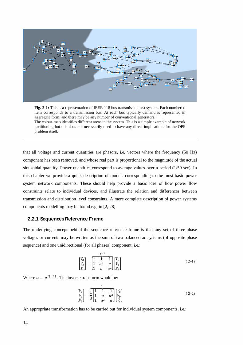
Fig. 2-1: This is a representation of IEEE-118 bus transmission test system. Each numbered item corresponds to a transmission bus. At each bus typically demand is represented in aggregate form, and there may be any number of conventional generators. The colour-map identifies different areas in the system. This is a simple example of network partitioning but this does not necessarily need to have any direct implications for the OPF problem itself.

15
푉 = 푧 퐼 ↔ 푇푉 = 푇푧 푇 푇퐼 ( 2–3)
Finally, as far as power is concerned:
푆 = 푉 퐼∗ = 푉 (푇 ) (푇 )∗퐼∗ = 3푉 퐼∗ ( 2–4)
As will be seen in the following sections, if a device is built to be symmetrical in terms of the
three phases, this transform can significantly simplify the equations that describe the device. Note
that symmetry in terms of voltage implies voltages of equal magnitude in each phase, with the
relative phase angle difference between phases being 120°.
2.2.2 Overhead Lines Impedance
The typical low voltage distribution line consists of 4 conductors / cables. For each individual
conductor resistance is an inherent frequency-dependent characteristic, while inductance depends
on the geometry of the conductors’ placement. In complex matrix notation, based on Fig. 2-2 the
following relation stands:
⎣⎢⎢⎢⎡Δ푉Δ푉Δ푉Δ푉 ⎦
⎥⎥⎥⎤
=
푧 푧 푧 푧푧 푧 푧 푧푧 푧 푧 푧푧 푧 푧 푧
퐼퐼퐼퐼
( 2–5)
For e.g. underground cable systems more equations would be required to account for the multiple
neutral wires. Under the assumption that the ground resistance between the two ends of the line
is negligible then 푉 ≈ 푉 = 0 and consequently 퐼 = −푧 (푧 퐼 + 푧 퐼 + 푧 퐼 ).
Substituting this into the above equations results in:
Δ푉Δ푉Δ푉
=
⎣⎢⎢⎢⎡ 푧 − 푧 − 푧 −
푧 − 푧 − 푧 −
푧 − 푧 − 푧 − ⎦⎥⎥⎥⎤ 퐼퐼퐼
( 2–6)
This is known as Kron’s reduction [28]. If the line is transposed then all diagonal elements are
equal (푧 ) and so are the off-diagonal elements (푧 ). Applying the symmetrical components
transform under this assumption yields:
Δ푉Δ푉Δ푉
=푧 + 2푧 0 0
0 푧 − 푧 00 0 푧 − 푧
퐼퐼퐼
( 2–7)
In case only positive and zero sequence resistances are known for a line, the approximate
primitive impedance model (2-6) may be derived by working backwards from (2-7). For unequal
diagonal and off-diagonal components in (2-6) the off-diagonal elements in (2-7) would be non-
zero. In distribution networks, given the limited length and fixed geometry this is often the case.
On the contrary, at the transmission level the opposite is always assumed to be true. Note that
16
typical generating systems in normal operation may be assumed to produce voltage in the positive
sequence only. Furthermore, all three-phase devices (generators, motors, transformers, etc.) are
built to be symmetrical, i.e. they introduce no coupling between sequences. If we were to assume
that the load is also balanced (e.g. a set of equal resistances connected to ground), then it should
be clear form (2-7) that the currents in zero and negative sequence would be equal to 0. This is a
common assumption when solving problems at the transmission level, and as such when writing
the network equations one needs only consider the positive sequence part.
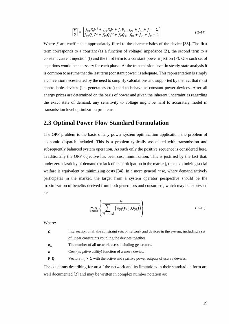
2.2.3 Transformers
Let us assume the general 3-phase unconnected transformer case as seen on Fig. 2-3. The
associated equations excluding dynamics in a per unit system with base voltage ratio that of the
transformer voltage ratio (tap effect included) are [29]:
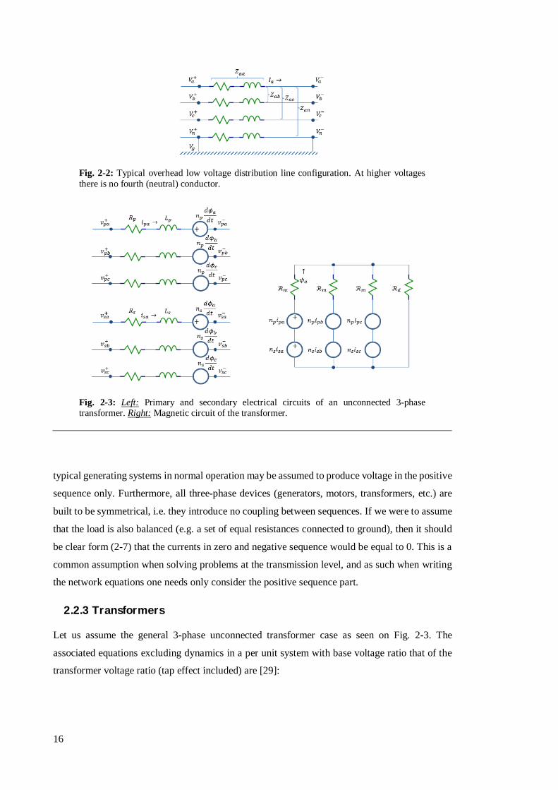
Fig. 2-2: Typical overhead low voltage distribution line configuration. At higher voltages there is no fourth (neutral) conductor.
Fig. 2-3: Left: Primary and secondary electrical circuits of an unconnected 3-phase transformer. Right: Magnetic circuit of the transformer.

17
⎣⎢⎢⎢⎢⎢⎢⎢⎢⎡Δ푉Δ푉Δ푉Δ푉Δ푉Δ푉
000 ⎦
⎥⎥⎥⎥⎥⎥⎥⎥⎤
=
⎣⎢⎢⎢⎢⎢⎢⎢⎢⎡푧 0 0 0 0 0 푗휔 0 00 푧 0 0 0 0 0 푗휔 00 0 푧 0 0 0 0 0 푗휔0 0 0 푧 0 0 푗휔 0 00 0 0 0 푧 0 0 푗휔 00 0 0 0 0 푧 0 0 푗휔−1 0 0 −1 0 0 ℛ + ℛ ℛ ℛ0 −1 0 0 −1 0 ℛ ℛ +ℛ ℛ0 0 −1 0 0 −1 ℛ ℛ ℛ + ℛ ⎦
⎥⎥⎥⎥⎥⎥⎥⎥⎤
⎣⎢⎢⎢⎢⎢⎢⎢⎢⎡푖푖푖푖푖푖휓휓휓 ⎦⎥⎥⎥⎥⎥⎥⎥⎥⎤
( 2–8)
Where:
푧 , 푧 Primary and secondary circuit impedance (resistance and leakage inductance).
휓 Magnetic flux.
ℛ Magnetic reluctance. For a transformer bank ℛ = 0 while for a five-legged transformer
ℛ = 푅 .
Applying the symmetrical components transform yields:
⎣⎢⎢⎢⎢⎢⎢⎢⎢⎡Δ푉Δ푉Δ푉Δ푉Δ푉Δ푉
000 ⎦
⎥⎥⎥⎥⎥⎥⎥⎥⎤
=
⎣⎢⎢⎢⎢⎢⎢⎢⎢⎡푧 0 0 0 0 0 푗휔 0 00 푧 0 0 0 0 0 푗휔 00 0 푧 0 0 0 0 0 푗휔0 0 0 푧 0 0 푗휔 0 00 0 0 0 푧 0 0 푗휔 00 0 0 0 0 푧 0 0 푗휔−1 0 0 −1 0 0 ℛ + 3ℛ 0 00 −1 0 0 −1 0 0 ℛ 00 0 −1 0 0 −1 0 0 ℛ ⎦
⎥⎥⎥⎥⎥⎥⎥⎥⎤
⎣⎢⎢⎢⎢⎢⎢⎢⎢⎡푖푖푖푖푖푖휓휓휓 ⎦⎥⎥⎥⎥⎥⎥⎥⎥⎤
( 2–9)
Eliminating the magnetic flux equations yields:
⎣⎢⎢⎢⎢⎢⎡Δ푉Δ푉Δ푉Δ푉Δ푉Δ푉 ⎦
⎥⎥⎥⎥⎥⎤
=
⎣⎢⎢⎢⎢⎢⎢⎢⎢⎢⎢⎢⎢⎡푧 +
푗휔ℛ + 3ℛ 0 0
푗휔ℛ + 3ℛ 0 0
0 푧 +푗휔ℛ 0 0
푗휔ℛ 0
0 0 푧 +푗휔ℛ 0 0
푗휔ℛ
푗휔ℛ + 3ℛ 0 0 푧 +
푗휔ℛ + 3ℛ 0 0
0푗휔ℛ 0 0 푧 +
푗휔ℛ 0
0 0푗휔ℛ 0 0 푧 +
푗휔ℛ ⎦
⎥⎥⎥⎥⎥⎥⎥⎥⎥⎥⎥⎥⎤
⎣⎢⎢⎢⎢⎢⎡퐼퐼퐼퐼퐼퐼 ⎦⎥⎥⎥⎥⎥⎤
( 2–10)
Given that the leakage impedances are very small compared to the impedance representing the
magnetic circuit they may be placed on the same side and replaced by 푦 = 푧 + 푧 . Considering
also that typically ℛ ≈ 0 one may write:

18
⎣⎢⎢⎢⎢⎢⎡퐼퐼퐼퐼퐼퐼 ⎦⎥⎥⎥⎥⎥⎤
=
⎣⎢⎢⎢⎢⎢⎡푦 0 0 −푦 0 00 푦 0 0 −푦 00 0 푦 0 0 −푦
−푦 0 0 푦 +3ℛ푗휔 0 0
0 −푦 0 0 푦 00 0 −푦 0 0 푦 ⎦
⎥⎥⎥⎥⎥⎤
⎣⎢⎢⎢⎢⎢⎡Δ푉Δ푉Δ푉Δ푉Δ푉Δ푉 ⎦
⎥⎥⎥⎥⎥⎤
( 2–11)
Note that this last equation does not account for the connections between the windings. Further
details may be found in [30]. One further assumption can be that ℛ ≈ 0, due to the fact that
under normal operating conditions any associated leakage currents would be very small compared
to the current fed to the load or a short-circuit. It should be noted however that for wye - grounded
wye connections this approximation would result in underestimating the zero sequence current
[29]. Nevertheless, in practice more often than not distribution transformer connections are
grounded wye – delta. Note that an off-nominal tap position could be represented by the same set
of equations by substituting Δ푉 by 푛 Δ푉 and 퐼 by 퐼 /푛 , where 푛 the off-
nominal tap ratio. An alternative approach would be using pi-equivalent models as in [31].
2.2.4 Phase Configurations & Generic Device Model
When it comes to single-phase devices things are simple, as there are typically two connectors
carrying power: phase and neutral. However, considering the individual circuit corresponding to
any three-phase device (e.g. the transformer of Fig. 2-3) then there are several possibilities in
terms of connection. The most common ones are the wye and delta configurations which establish
the following relations between the phase circuit current and voltage in the device (designated
with the index d) and the actual phase current injection and voltage in the network (designated
with the index i):
푉 ,푉 ,푉 ,
=1 0 00 1 00 0 1
푉 ,푉 ,푉 ,
,퐼 ,퐼 ,퐼 ,
=1 0 00 1 00 0 1
퐼 ,퐼 ,퐼 ,
푤푦푒 푐표푛푛푒푐푡푖표푛 ( 2–12)
푉 ,푉 ,푉 ,
=1 −1 00 1 −1−1 0 1
푉 ,푉 ,푉 ,
,퐼 ,퐼 ,퐼 ,
=1 0 −1−1 1 00 −1 1
퐼 ,퐼 ,퐼 ,
푑푒푙푡푎 푐표푛푛푒푐푡푖표푛 ( 2–13)
These equations have to be incorporated in the impedance / admittance matrix representing each
device.
Regarding the end-user devices themselves different equations would represent different devices
(e.g. lighting or induction motors). However more often than not, the exact nature of the connected
devices is not typically known. Even if it is actually known, the exact models may be overly
complex for optimization or simulation applications. A model commonly used and assumed to be
sufficiently accurate for any device (or set of devices) would be the ZIP representation [32]:
19
푃푄 =
푓 푃 푉 + 푓 푃 푉 + 푓 푃 ; 푓 + 푓 + 푓 = 1푓 푄 푉 + 푓 푄 푉 + 푓 푄 ; 푓 + 푓 + 푓 = 1 ( 2–14)
Where 푓 are coefficients appropriately fitted to the characteristics of the device [33]. The first
term corresponds to a constant (as a function of voltage) impedance (Z), the second term to a
constant current injection (I) and the third term to a constant power injection (P). One such set of
equations would be necessary for each phase. At the transmission level in steady-state analysis it
is common to assume that the last term (constant power) is adequate. This representation is simply
a convention necessitated by the need to simplify calculations and supported by the fact that most
controllable devices (i.e. generators etc.) tend to behave as constant power devices. After all
energy prices are determined on the basis of power and given the inherent uncertainties regarding
the exact state of demand, any sensitivity to voltage might be hard to accurately model in
transmission level optimization problems.
2.3 Optimal Power Flow Standard Formulation
The OPF problem is the basis of any power system optimization application, the problem of
economic dispatch included. This is a problem typically associated with transmission and
subsequently balanced system operation. As such only the positive sequence is considered here.
Traditionally the OPF objective has been cost minimization. This is justified by the fact that,
under zero elasticity of demand (or lack of its participation in the market), then maximizing social
welfare is equivalent to minimizing costs [34]. In a more general case, where demand actively
participates in the market, the target from a system operator perspective should be the
maximization of benefits derived from both generators and consumers, which may be expressed
as:
min[퐏;퐐]∈푪
푢{ } 퐏( ),퐐( )∈{ ,..., }
( 2–15)
Where:
푪 Intersection of all the constraint sets of network and devices in the system, including a set
of linear constraints coupling the devices together.
푛 The number of all network users including generators.
푢 Cost (negative utility) function of a user / device.
퐏,퐐 Vectors 푛 × 1 with the active and reactive power outputs of users / devices.
The equations describing for area i the network and its limitations in their standard ac form are
well documented [2] and may be written in complex number notation as:

20
퐶 { } =
⎩⎨
⎧퐒 { } = 푑푖푎푔 퐕{ } 퐘{ }퐕{ }∗
퐕{ } ≤ 퐕{ } ≤ 퐕{ }
퐘 { }퐕{ } ≤ 퐈 { } ⎭⎬
⎫ 푖 ∈ [1,푛 ] ( 2–16)
퐘{ }( , ) =
⎩⎪⎨
⎪⎧ −
1푟 + 푗푥 : 푖푓 푙 ≠ 푗
1푟 + 푗푥 +
푗푏2
∈[ , ]
: 푖푓 푙 = 푗 푙, 푗 ∈ [1,푛 ] ( 2–17)
퐘 { }( , ) =
⎩⎨
⎧1
푟 + 푗푥 : 푖푓 푙푖푛푒 푙 푠푡푎푟푡푠 푓푟표푚 푏푢푠 푗
−1푟 + 푗푥 : 푖푓 푙푖푛푒 푙 푒푛푑푠 표푛 푏푢푠 푗
푙 ∈ [1,푛 ], 푗 ∈ [1,푛 ] ( 2–18)
Where:
푛 The number of all network buses in the area.
푛 The number of all network areas.
푛 The number of all lines in the area.
푟 ,푥 Line resistance and inductance.
푟 ,푥 ,푏 Total resistance, inductance and admittance between buses i and j.
푽( ) Complex voltages 푛 × 1 vector. The voltages may be represented either in polar
(퐕( ) = 퐕( ) 푒 ∠퐕( ) ) or rectangular (퐕( ) = 푟푒푎푙 퐕( ) + 푗 ∙ 푖푚푎푔 퐕( ) form.
푺 ( ) Apparent power injection 푛 × 1 vector.
푰 ( ) Lines maximum current capacities 푛 × 1 vector.
The equations in (2-16) describe respectively the power balance constraints, voltage constraints
and line capacity constraints. Note that it is quite common to represent the latter in terms of
transferred power. However, placing the constraint on line current simplifies calculations and it
is closer to the actual physical constraints in the system (i.e. current is the quantity directly
associated with the thermal limitations of the conductors; transferred power may be alternatively
used on the assumption of a given voltage value at the end of the line). The above equations,
group together the positive sequence constraints of the form (2-7) for all network components.
The next subset of typical constraints is that of demand or generation:
퐶 / { } =
⎩⎪⎨
⎪⎧ 푢{ } = 푐 { }퐏( ) + 푐 { }퐏( )
퐏( ) ≤ 퐏( ) ≤ 퐏( )
푄{ } ≤ 퐐( ) ≤ 푄{ } 표푟 퐐( ) = 푓 { } 퐏( ) ⎭⎪⎬
⎪⎫
푖 ∈ [1,푛 ] ( 2–19)
Where:
푐 , 푐 Variable costs coefficients for generators. For demand 푐 = 0, 푐 > 0 and equal to the
value a client associates with energy use. It can be thought of as an equivalent to the value
of lost load (VOLL) which is assumed to be about 100 times the value of energy at peak
demand.

21
푓 Function of reactive power as a function of active power. For e.g. demand operating at a
fixed power factor this is simply a linear function. For devices where reactive power is
independently controlled from active power, this function does not apply and only
reactive power limits are taken into account.
Finally, the linear set of constraints coupling network and devices together may be described as:
퐶 = {퐂 퐔 = 0,퐂 퐔 = 0,퐂 퐔 = 0} ( 2–20)
The vectors 푈 ,푈 ,푈 are derived from the concatenation of 퐏( ) and 푟푒푎푙 퐒 ( ) , 퐐( ) and
푖푚푎푔 퐒 ( ) , and 퐕( ) respectively. Matrices 퐂 ,퐂 have elements of 1, 0, -1 establishing variables
equality at the coupling nodes.
2.4 Branch Flow Model (Radial Networks Only)
Transmission networks are typically meshed (i.e. some nodes may be connected through more
than one path), while distribution networks typically have a tree/radial structure (i.e. any two
nodes are connected through exactly one path). If the network has a radial structure, it is possible
to use a different set of equations, i.e. the branch flow model initially proposed in [35]. Assuming
balanced operation for any line from bus i to j, for the power 푇 and 푇 drawn from the two ends
of the line we have:
푇 + 푇 = (푟 + 푗푥) |퐼| ( 2–21)
With 푇 = 푇 + 푗푇 for the voltages we have the following equation:
푉 = 푉 − 푧퐼 = 푉 − 푧푇∗
푉∗ ⇒ 푉푉 = ||푉 | − 푧푇∗| ⇒
⇒ |푉 | |푉 | = |푉 | − 2|푉 | 푟푇 + 푥푇 + (푟 + 푥 ) 푇 + 푇 ( 2–22)
This effectively removes the bus voltage angle from the equations. Note that as indicated in [36,
37] only one of the voltage magnitude solutions to this quadratic voltage drop equation can be
within the range allowed by typical voltage constraints. Furthermore, as reference [38] proves,
there always exists an inverse projection that allows the recovery of voltage angles for radial
networks. Generalising the overall equations of the network may be written as:
퐶 =
⎩⎪⎨
⎪⎧
퐒 = 퐘 퐓−퐘 퐓− 풀 풍퐘 − 퐘 풗 = −2 푑푖푎푔{풓}퐓 + 푑푖푎푔{풙}퐓 + 푑푖푎푔{풛}풍
퐘 풗 ∙ 푑푖푎푔{풍} = |퐓|ퟐ
풗 ≤ 풗 ≤ 풗풍 ≤ 풍 ⎭
⎪⎬
⎪⎫
( 2–23)
Where:
풍 A 푛 × 1 vector of squared line current magnitude.
풗 A 푛 × 1 vector of squared bus voltage magnitude.

22
퐓 A 푛 × 1 vector of line power flows.
The two first equations in the constraint set (2-23) are simply (2-21) and (2-22) respectively
written for the whole network. While this form offers a clearer representation of line flows, due
to the third constraint, power flow equations are still non-convex and they do not appear to directly
offer any significant benefit compared to the initial ac formulation. As such in this work the
constraint set in (2-2) is preferred to (2-9).
2.5 DC Load Flow (Transmission Only)
The full AC equations may be significantly simplified under the following assumptions [2]:
Bus voltages are assumed to be equal to 1 푝.푢. and the equations related to reactive power are
neglected.
Branch resistances are much smaller than branch reactances and may be neglected. Shunt
reactances to the ground may also be neglected.
Voltage angle differences between two connected buses are assumed to be small and as a
consequence 푠푖푛훿 ≈ 훿 − 훿 and 푐표푠훿 ≈ 1.
The apparent power transferred between buses 푖 and 푗 through transmission line 푘 is equal to:
푆 = 푉푉 − 푉 ∗
푍∗ = 푉푒푉푒 − 푉푍 푒 =
1푍 푉 푒 − 푉푉 푒 ( 2–24)
Consequently, under the aforementioned assumptions the real power is given by:
Re 푆 =1푍 푉 푐표푠(휃 )−푉푉푐표푠 휃 + 훿 ≈
훿 − 훿푍 ( 2–25)
This yields a linear set of power balance equations of the following form:
퐏 = 퐁훅 ( 2–26)
Where:
훅 A 푛 × 1 bus angles vector.
퐁 The simplified bus admittance matrix. Where 1/퐁( , ) = 1 푦⁄ = ∑(푗푥 ),푘 ∈ 푁 → , and
퐁( , ) = −∑ 퐁( ),.., .
This simplified set of equations cannot be used in cases where voltage and reactive power play a
defining role. Also the second assumption is not valid for distribution networks due to their high
푟/푥 ratio. However, it gives an adequately good representation of active power flows in the
system, while offering a significant reduction in computational cost. Furthermore, these
constraints are obviously convex.
The above formulation may be easily extended to take transmission losses into account. Losses
over a transmission line may be approximated based on the following equation [39]:
23
푃 , = 푆 − 푆 =푐표푠(휃 )푍 푉 + 푉 − 2푉푉푐표푠 훿 ≈
≈2푟푍 1− 푐표푠 훿 ≈
4푟푥 푠푖푛
훿2 ≈ 푟 Re 푆
( 2–27)
These losses may be distributed equally to each of the connected buses as indicated in [40]. An
iterative approach to take losses into account, as well as a comparison with AC OPF with respect
to calculated marginal prices may be found in [41]. The comparison indicates that in case the two
methods identify a different marginal unit due to the approximation error, then the marginal costs
differences can be significant. Note that with loses included the resulting problem becomes again
non-convex though still easier to solve than the full AC problem.
The fact that there is no way to represent voltages in DC OPF implies that it is probably unsuitable
for any application at the distribution level. On the transmission level while similar models could
appear as part of a decoupled load-flow formulation, by itself there is little value to using this
model, unless one can be certain that: 1) voltages are not a problem; 2) in terms of marginal prices
the approximation of losses is acceptable. In any case we still opt to use the original set of (2.2)
rather than this formulation.
2.6 Convex Relaxations
As mentioned the set 퐶 is non-convex. This implies that in the corresponding optimization
problem exist local minima and depending on the starting point of the optimization algorithm
different solutions could be reached. The following subsections present various convex
relaxations of the initial problem and discuss their applicability.
2.6.1 Semi Definite Programming
A reformulation of the OPF problem into a semi definite programming (SDP) form seems to have
first been made in [42], while a more concise description of the approach may be found in [43,
44]. The underlying concept is that if 풆 , … ,풆 the basis vectors of ℝ , then the power balance
equations at any given node may be written as:
푆( ) = 푡푟푎푐푒 퐘퐞 퐞 퐖 , 푖 ∈ 푁 ( 2–28)
With the additional constraints:
퐖 ≽ 0, 푟푎푛푘{퐖} = 1 ( 2–29)
The sign ≽ indicates that 퐖 is a positive semi-definite matrix (i.e. its eigenvalues are all non-
negative). Under the constraints (2-29) there is a unique decomposition 퐖 = 퐕퐕 . However, the
rank constraint makes the problem non-convex, and subsequently a convex relaxation may be
reached by simply dropping this constraint. The authors in the aforementioned papers derive
24
necessary conditions for the relaxation to be tight, and they conjecture that those are fulfilled as
long as the resistive part of the system (i.e. the graph induced by 푟푒푎푙{풀}) is strongly connected
(i.e. there exists a path between any two nodes of the graph). In some IEEE test systems this
required the addition of a small resistance, on the order of 10 , to any transmission component
having a resistance lower than that. Reference [45] suggests that the SDP relaxation may be used
also in the presence of more complex constraints, such as those involved in security constrained
power flow, while [46] suggests that it is always tight in radial networks. It should be noted
however that in case of negative marginal prices or very tight transmission constraints the SDP
relaxation can fail [47]. Following these results subsequent papers [48, 49] further investigated
the necessary conditions under which the SDP relaxation may be used, without however being
conclusive regarding its range of application.
2.6.2 Conic Programming
Going back to the set of branch flow equations convexification is possible if the current equation
for line k was relaxed to an inequality:
푙 ≥푃 + 푄
푣⟺ 푙 + 푣 ≥
2푃2푄푙 − 푣
( 2–30)
The equation on the right is a second-order cone (SOC) set of constraints which is known to be
convex. Intuitively losses over a power line will ensure that 푙 remains at its lower bound at the
optimal solution. Reference [38] investigates the conditions where this relaxation is tight and
further proves when voltage angles may be recovered. More specifically let 퐺 be a graph
describing the network and for any spanning tree 푇(푁,퐸 ) of 퐺, let 푩 be the incidence matrix
of lines included in 푇 and 푩 the incidence matrix of lines not included in 푇. Bus angles may be
similarly partitioned into two sets 휹 and 휹 . If 푚표푑(푩 푩 휹 − 휹 , 2휋) = 0 then there is a
unique solution 휹∗ = 푩 휹 . This relation always holds for radial networks. In meshed networks,
assuming phase shifters are placed in branches outside the spanning tree, then the angle recovery
condition becomes 푚표푑(푩 푩 (휹 − 흓 ) − (휹 − 흓 ), 2휋) = 0, where 흓 are angles
introduced by the phase shifters [50]. For a suitable selection of the latter the angle recovery
condition always holds. Of course having phase shifters at all the right places for this condition
to hold cannot be expected in real networks as their installation entails a significant cost.
It should be noted that according to [51] there exists a one to one mapping between the solution
set of this relaxation and the SDP based one. However, perhaps the most important implication
of this is that both relaxations share the same issues in terms of applicability. Thus an extended
discussion on the conditions under which the conic relaxation of the branch flow model is exact
in radial networks may be found in [52]. The derived conditions are shown to be valid for two
25
real distribution networks. However, these conditions would have to be checked for each
particular network and general applicability should not be taken for granted. Another conic
relaxation approach for distribution networks may also be found in [53, 54] however these appear
to be rather restrictive in terms of problem formulation.
While convex relaxations represent a very interesting mathematical work in power systems they
are still at an early stage of development. At the time of writing it was not deemed as a good idea
to use such models as: 1) they require certain conditions to be fulfilled in order to work which are
not fully clarified in current literature; 2) even when they work the computational burden is
typically much higher than that involved in solving the original non-convex model through e.g.
an interior point method. The standard ac formulation still appears to be the better option. Further
information regarding the SDP and SOC relaxations, as well as the relation between them, may
also be found in [55].
2.7 Unbalanced Optimal Power Flow Generic Formulation
In contrast to transmission which may be assumed to be always operating in a balanced manner
(i.e. same amplitude of voltage and current in all three phases), distribution networks are almost
always unbalanced. As such, especially when considering electric vehicles which could represent
significant single phase loads, optimizing the network considering a full unbalanced load flow
might be a requirement. As discussed earlier, in terms of constraints modelling there are two
possibilities: 1) express the constraints in the 3-phase reference frame; 2) convert the 3-phase
equations into the so-called sequence reference frame. As shown earlier, the sequence
transformation effectively replaces the 3-phase quantities by three equivalent ones, which for fully
balanced devices and systems may be solved independently. For unbalanced systems the result is
usually a sparser constraints representation. Due to this fact a number of papers advocate the use
of symmetrical components [56] or attempt to exploit the sequence components structure [57] in
order to achieve faster solutions for power flow problems. However, when it comes to optimal
power flow, available references are more limited, and what the ideal formulation is remains
unclear.
In terms of OPF a number of papers use sequence components, e.g. [58] which proposes a multi-
objective chance constrained optimization model for distribution networks. In terms of network
equations, the paper states that due to the weak coupling sequences may be independently solved.
This would be imprecise however when a significant number of unbalanced loads is present. The
same comment applies to [59], which focuses on voltage-converter interfaced generation – this is
represented simply by a voltage source in the positive sequence and zero resistance in the
remaining sequences.
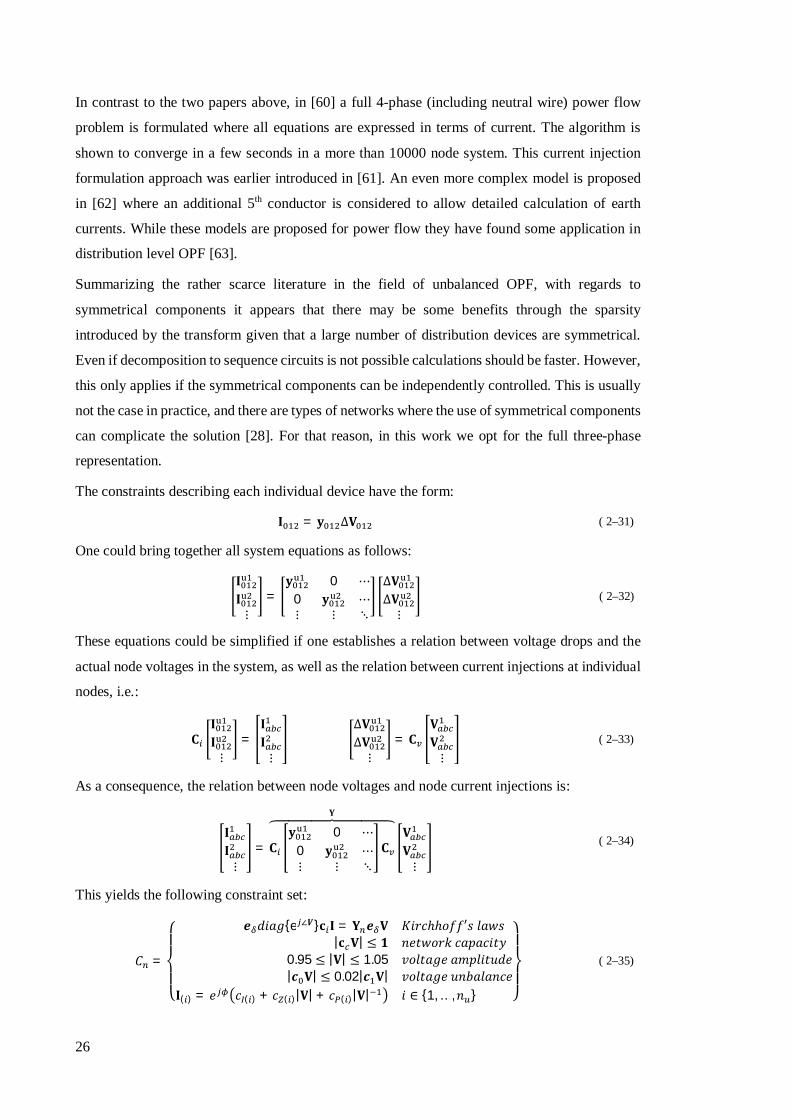
26
In contrast to the two papers above, in [60] a full 4-phase (including neutral wire) power flow
problem is formulated where all equations are expressed in terms of current. The algorithm is
shown to converge in a few seconds in a more than 10000 node system. This current injection
formulation approach was earlier introduced in [61]. An even more complex model is proposed
in [62] where an additional 5th conductor is considered to allow detailed calculation of earth
currents. While these models are proposed for power flow they have found some application in
distribution level OPF [63].
Summarizing the rather scarce literature in the field of unbalanced OPF, with regards to
symmetrical components it appears that there may be some benefits through the sparsity
introduced by the transform given that a large number of distribution devices are symmetrical.
Even if decomposition to sequence circuits is not possible calculations should be faster. However,
this only applies if the symmetrical components can be independently controlled. This is usually
not the case in practice, and there are types of networks where the use of symmetrical components
can complicate the solution [28]. For that reason, in this work we opt for the full three-phase
representation.
The constraints describing each individual device have the form:
퐈 = 퐲 Δ퐕 ( 2–31)
One could bring together all system equations as follows:
퐈퐈⋮
=퐲 0 ⋯
0 퐲 ⋯⋮ ⋮ ⋱
Δ퐕Δ퐕⋮
( 2–32)
These equations could be simplified if one establishes a relation between voltage drops and the
actual node voltages in the system, as well as the relation between current injections at individual
nodes, i.e.:
퐂퐈퐈⋮
=퐈퐈⋮
Δ퐕Δ퐕⋮
= 퐂퐕퐕⋮
( 2–33)
As a consequence, the relation between node voltages and node current injections is:
퐈퐈⋮
= 퐂퐲 0 ⋯
0 퐲 ⋯⋮ ⋮ ⋱
퐂
퐘
퐕퐕⋮
( 2–34)
This yields the following constraint set:
퐶 =
⎩⎪⎨
⎪⎧ 풆 푑푖푎푔{e ∠푽}퐜 퐈 = 퐘 풆 퐕 퐾푖푟푐ℎℎ표푓푓′푠 푙푎푤푠
|퐜 퐕| ≤ ퟏ 푛푒푡푤표푟푘 푐푎푝푎푐푖푡푦0.95 ≤ |퐕| ≤ 1.05 푣표푙푡푎푔푒 푎푚푝푙푖푡푢푑푒|풄 퐕| ≤ 0.02|풄 퐕| 푣표푙푡푎푔푒 푢푛푏푎푙푎푛푐푒
퐈( ) = 푒 푐 ( ) + 푐 ( )|퐕| + 푐 ( )|퐕| 푖 ∈ {1, … ,푛 } ⎭⎪⎬
⎪⎫
( 2–35)
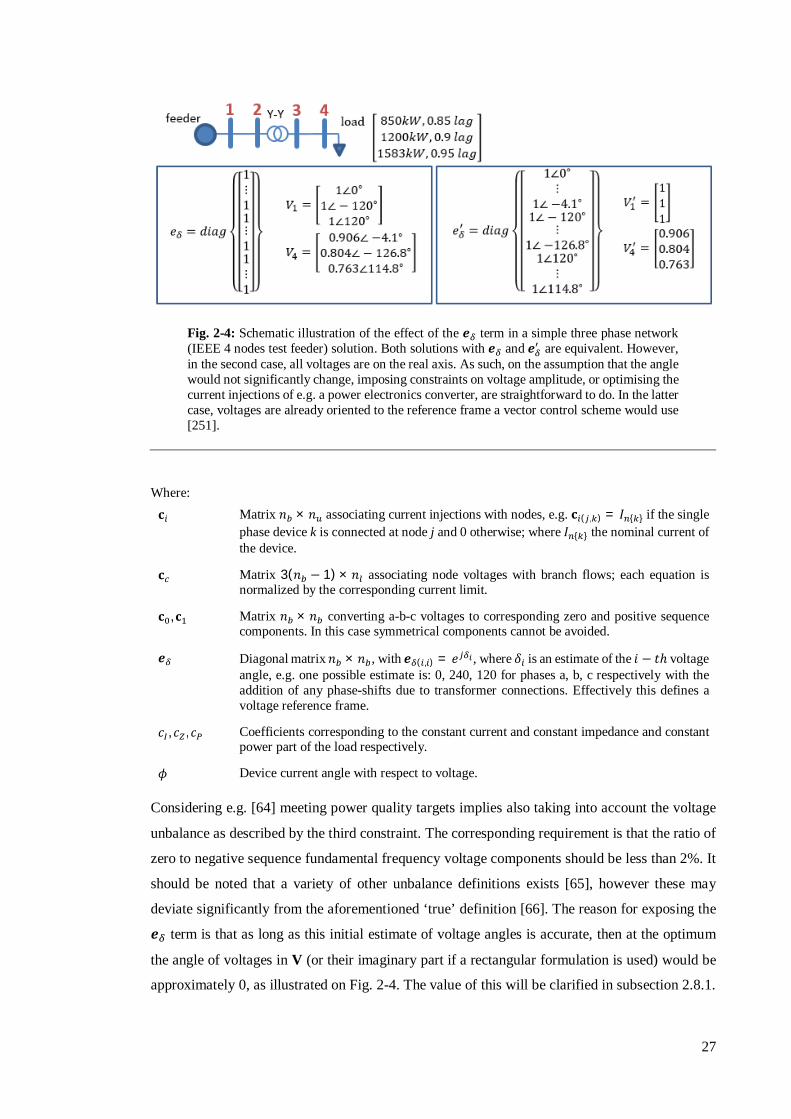
27
Where: 퐜 Matrix 푛 × 푛 associating current injections with nodes, e.g. 퐜 ( , ) = 퐼 { } if the single
phase device k is connected at node j and 0 otherwise; where 퐼 { } the nominal current of the device.
퐜 Matrix 3(푛 − 1) × 푛 associating node voltages with branch flows; each equation is normalized by the corresponding current limit.
퐜 , 퐜 Matrix 푛 × 푛 converting a-b-c voltages to corresponding zero and positive sequence components. In this case symmetrical components cannot be avoided.
풆 Diagonal matrix 푛 × 푛 , with 풆 ( , ) = 푒 , where 훿 is an estimate of the 푖 − 푡ℎ voltage angle, e.g. one possible estimate is: 0, 240, 120 for phases a, b, c respectively with the addition of any phase-shifts due to transformer connections. Effectively this defines a voltage reference frame.
푐 , 푐 , 푐 Coefficients corresponding to the constant current and constant impedance and constant power part of the load respectively.
휙 Device current angle with respect to voltage.
Considering e.g. [64] meeting power quality targets implies also taking into account the voltage
unbalance as described by the third constraint. The corresponding requirement is that the ratio of
zero to negative sequence fundamental frequency voltage components should be less than 2%. It
should be noted that a variety of other unbalance definitions exists [65], however these may
deviate significantly from the aforementioned ‘true’ definition [66]. The reason for exposing the
풆 term is that as long as this initial estimate of voltage angles is accurate, then at the optimum
the angle of voltages in V (or their imaginary part if a rectangular formulation is used) would be
approximately 0, as illustrated on Fig. 2-4. The value of this will be clarified in subsection 2.8.1.
Fig. 2-4: Schematic illustration of the effect of the 풆 term in a simple three phase network (IEEE 4 nodes test feeder) solution. Both solutions with 풆 and 풆 are equivalent. However, in the second case, all voltages are on the real axis. As such, on the assumption that the angle would not significantly change, imposing constraints on voltage amplitude, or optimising the current injections of e.g. a power electronics converter, are straightforward to do. In the latter case, voltages are already oriented to the reference frame a vector control scheme would use [251].

28
2.8 Current Injection Approximations (Distribution Only)
Considering a balanced network, let us now calculate the current corresponding to this load with
푉 = |푉 + 푗푉 | under the assumption that 푉 ≈ 푉 :
퐼 =푃 − 푗푄푉 − 푗푉 =
푓 푃 − 푗푓 푄푉 − 푗푉 푉 +
푓 푃 − 푗푓 푄푉 − 푗푉 푉 +
푓 푃 − 푗푓 푄푉 − 푗푉 ≈
≈ 푓 푃 − 푗푓 푄 (푉 + 푗푉 ) + 푓 푃 − 푗푓 푄 +푓 푃 − 푗푓 푄
푉
( 2–36)
This assumption is also followed in [67] which focuses on the distribution level, dropping
however the constant power term. Subsequently the power flow equations may be written as:
퐶 =퐈 + 퐘∗(퐕풓 − 푗퐕풊) = 퐘∗(퐕풓 − 푗퐕풊)
퐕 ≤ 퐕풓 ≤ 퐕−퐈 ≤ 퐘 퐈 ≤ 퐈
( 2–37)
Assuming that only the current injection part is variable then the optimal power flow constraints
are significantly simplified.
Reference [68] also uses a current injection based formulation for the network and presents a
systematic approach to linearize the models for both loads and amplitude constraints using
rectangular coordinates for voltage. Disjunctive inequality constraints are used to represent load
controls, which are generally assumed to be discrete in nature. Overall the presented approach
yields a mixed integer linear programming problem of increased complexity, but suitable for most
optimization applications in distribution networks.
Modelling demand accurately in terms of power is perhaps of fundamental importance when
working within the context of an energy market where all payments are carried out on the basis
of power injections. However, when discussing about distribution networks at a level where
individuals are not exposed to a market, then this is not necessary. It is a fact after all that constant
power models used at the transmission level do not adequately model low voltage demand.
Overall a sensible approach could be to simply use the most mathematically simple model that
adequately captures the current-voltage relationship of any given connected device. Effectively if
all demand could be modelled as a current injection then the power flow constraints would be
convex.
2.8.1 Current Approximation Approach for Unbalanced Networks
The above assumption of a constant angle for voltage in terms of nodal current injections can
significantly simplify (2-35). However, it would unavoidably introduce an error (depending on
the angle) in terms of power output and potentially voltage. In this work we propose a novel
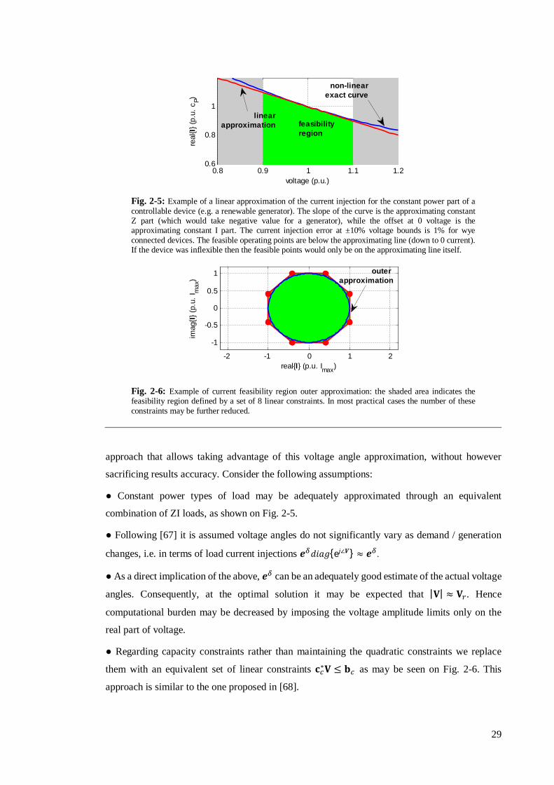
29
approach that allows taking advantage of this voltage angle approximation, without however
sacrificing results accuracy. Consider the following assumptions:
● Constant power types of load may be adequately approximated through an equivalent
combination of ZI loads, as shown on Fig. 2-5.
● Following [67] it is assumed voltage angles do not significantly vary as demand / generation
changes, i.e. in terms of load current injections 풆 푑푖푎푔{e푗∠푽} ≈ 풆 .
● As a direct implication of the above, 풆 can be an adequately good estimate of the actual voltage
angles. Consequently, at the optimal solution it may be expected that |퐕| ≈ 퐕 . Hence
computational burden may be decreased by imposing the voltage amplitude limits only on the
real part of voltage.
● Regarding capacity constraints rather than maintaining the quadratic constraints we replace
them with an equivalent set of linear constraints 퐜∗퐕 ≤ 퐛 as may be seen on Fig. 2-6. This
approach is similar to the one proposed in [68].
Fig. 2-5: Example of a linear approximation of the current injection for the constant power part of a controllable device (e.g. a renewable generator). The slope of the curve is the approximating constant Z part (which would take negative value for a generator), while the offset at 0 voltage is the approximating constant I part. The current injection error at ±10% voltage bounds is 1% for wye connected devices. The feasible operating points are below the approximating line (down to 0 current). If the device was inflexible then the feasible points would only be on the approximating line itself.
Fig. 2-6: Example of current feasibility region outer approximation: the shaded area indicates the feasibility region defined by a set of 8 linear constraints. In most practical cases the number of these constraints may be further reduced.
0.8 0.9 1 1.1 1.20.6
0.8
1
voltage (p.u.)re
al{I}
(p.u
. cP)
non-linearexact curve
linearapproximation feasibility
region
-2 -1 0 1 2
-1
-0.5
0
0.5
1
real{I} (p.u. Imax)
imag
{I} (p
.u. I
max
)
outer approximation
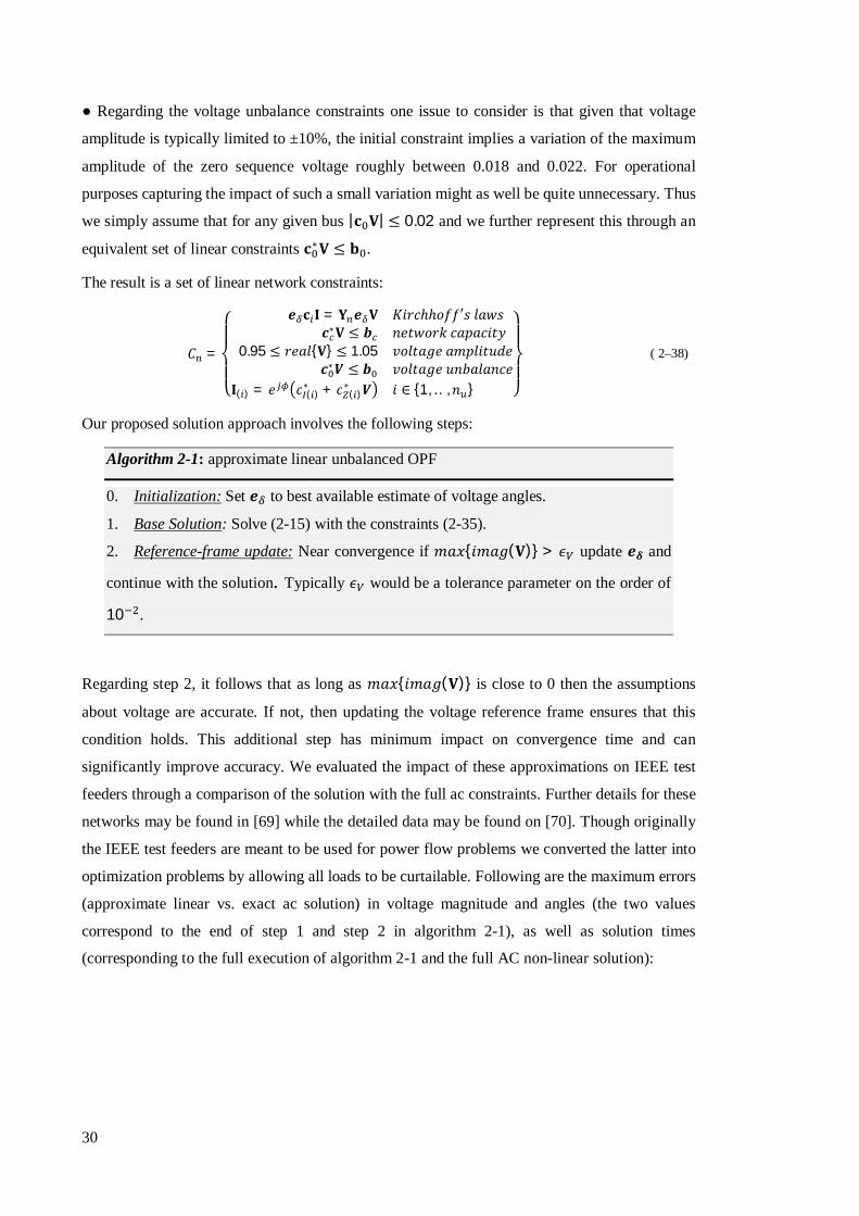
30
● Regarding the voltage unbalance constraints one issue to consider is that given that voltage
amplitude is typically limited to ±10%, the initial constraint implies a variation of the maximum
amplitude of the zero sequence voltage roughly between 0.018 and 0.022. For operational
purposes capturing the impact of such a small variation might as well be quite unnecessary. Thus
we simply assume that for any given bus |퐜 퐕| ≤ 0.02 and we further represent this through an
equivalent set of linear constraints 퐜∗퐕 ≤ 퐛 .
The result is a set of linear network constraints:
퐶 =
⎩⎪⎨
⎪⎧ 풆 퐜 퐈 = 퐘 풆 퐕 퐾푖푟푐ℎℎ표푓푓′푠 푙푎푤푠
풄∗퐕 ≤ 풃 푛푒푡푤표푟푘 푐푎푝푎푐푖푡푦0.95 ≤ 푟푒푎푙{퐕} ≤ 1.05 푣표푙푡푎푔푒 푎푚푝푙푖푡푢푑푒
풄∗푽 ≤ 풃 푣표푙푡푎푔푒 푢푛푏푎푙푎푛푐푒퐈( ) = 푒 푐 ( )
∗ + 푐 ( )∗ 푽 푖 ∈ {1, … , 푛 } ⎭
⎪⎬
⎪⎫
( 2–38)
Our proposed solution approach involves the following steps:
Algorithm 2-1: approximate linear unbalanced OPF
0. Initialization: Set 풆 to best available estimate of voltage angles.
1. Base Solution: Solve (2-15) with the constraints (2-35).
2. Reference-frame update: Near convergence if 푚푎푥{푖푚푎푔(퐕)} > 휖 update 풆휹 and
continue with the solution. Typically 휖 would be a tolerance parameter on the order of
10 .
Regarding step 2, it follows that as long as 푚푎푥{푖푚푎푔(퐕)} is close to 0 then the assumptions
about voltage are accurate. If not, then updating the voltage reference frame ensures that this
condition holds. This additional step has minimum impact on convergence time and can
significantly improve accuracy. We evaluated the impact of these approximations on IEEE test
feeders through a comparison of the solution with the full ac constraints. Further details for these
networks may be found in [69] while the detailed data may be found on [70]. Though originally
the IEEE test feeders are meant to be used for power flow problems we converted the latter into
optimization problems by allowing all loads to be curtailable. Following are the maximum errors
(approximate linear vs. exact ac solution) in voltage magnitude and angles (the two values
correspond to the end of step 1 and step 2 in algorithm 2-1), as well as solution times
(corresponding to the full execution of algorithm 2-1 and the full AC non-linear solution):
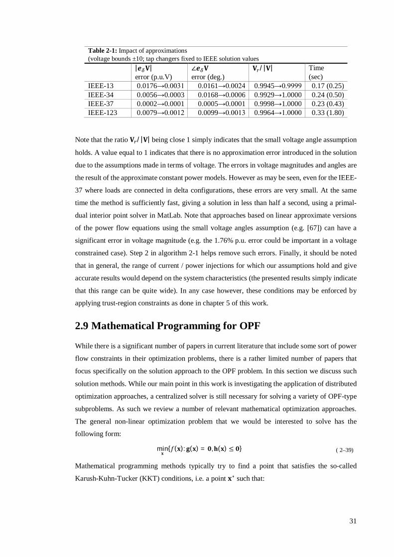
31
Table 2-1: Impact of approximations (voltage bounds ±10; tap changers fixed to IEEE solution values |풆 퐕|
error (p.u.V) ∠풆 퐕 error (deg.)
퐕 /|퐕| Time (sec)
IEEE-13 0.0176→0.0031 0.0161→0.0024 0.9945→0.9999 0.17 (0.25) IEEE-34 0.0056→0.0003 0.0168→0.0006 0.9929→1.0000 0.24 (0.50) IEEE-37 0.0002→0.0001 0.0005→0.0001 0.9998→1.0000 0.23 (0.43) IEEE-123 0.0079→0.0012 0.0099→0.0013 0.9964→1.0000 0.33 (1.80)
Note that the ratio 퐕 /|퐕| being close 1 simply indicates that the small voltage angle assumption
holds. A value equal to 1 indicates that there is no approximation error introduced in the solution
due to the assumptions made in terms of voltage. The errors in voltage magnitudes and angles are
the result of the approximate constant power models. However as may be seen, even for the IEEE-
37 where loads are connected in delta configurations, these errors are very small. At the same
time the method is sufficiently fast, giving a solution in less than half a second, using a primal-
dual interior point solver in MatLab. Note that approaches based on linear approximate versions
of the power flow equations using the small voltage angles assumption (e.g. [67]) can have a
significant error in voltage magnitude (e.g. the 1.76% p.u. error could be important in a voltage
constrained case). Step 2 in algorithm 2-1 helps remove such errors. Finally, it should be noted
that in general, the range of current / power injections for which our assumptions hold and give
accurate results would depend on the system characteristics (the presented results simply indicate
that this range can be quite wide). In any case however, these conditions may be enforced by
applying trust-region constraints as done in chapter 5 of this work.
2.9 Mathematical Programming for OPF
While there is a significant number of papers in current literature that include some sort of power
flow constraints in their optimization problems, there is a rather limited number of papers that
focus specifically on the solution approach to the OPF problem. In this section we discuss such
solution methods. While our main point in this work is investigating the application of distributed
optimization approaches, a centralized solver is still necessary for solving a variety of OPF-type
subproblems. As such we review a number of relevant mathematical optimization approaches.
The general non-linear optimization problem that we would be interested to solve has the
following form:
min퐱
{푓(퐱): 퐠(퐱) = ퟎ,퐡(퐱) ≤ ퟎ} ( 2–39)
Mathematical programming methods typically try to find a point that satisfies the so-called
Karush-Kuhn-Tucker (KKT) conditions, i.e. a point 퐱∗ such that:
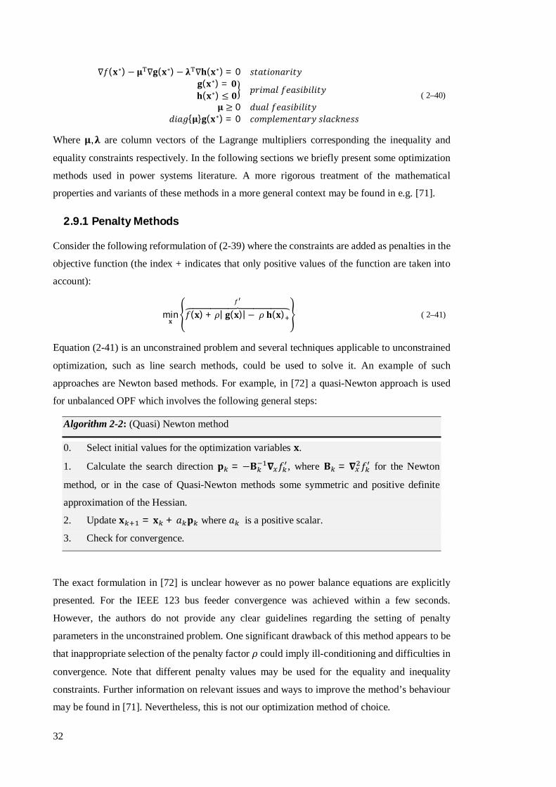
32
∇푓(퐱∗)− 훍 ∇퐠(퐱∗)− 훌 ∇퐡(퐱∗) = 0 푠푡푎푡푖표푛푎푟푖푡푦퐠(퐱∗) = ퟎ퐡(퐱∗) ≤ ퟎ 푝푟푖푚푎푙 푓푒푎푠푖푏푖푙푖푡푦
훍 ≥ 0 푑푢푎푙 푓푒푎푠푖푏푖푙푖푡푦푑푖푎푔{훍}퐠(퐱∗) = 0 푐표푚푝푙푒푚푒푛푡푎푟푦 푠푙푎푐푘푛푒푠푠
( 2–40)
Where 훍,훌 are column vectors of the Lagrange multipliers corresponding the inequality and
equality constraints respectively. In the following sections we briefly present some optimization
methods used in power systems literature. A more rigorous treatment of the mathematical
properties and variants of these methods in a more general context may be found in e.g. [71].
2.9.1 Penalty Methods
Consider the following reformulation of (2-39) where the constraints are added as penalties in the
objective function (the index + indicates that only positive values of the function are taken into
account):
min퐱
푓(퐱) + 휌| 퐠(퐱)|− 휌 퐡(퐱) ( 2–41)
Equation (2-41) is an unconstrained problem and several techniques applicable to unconstrained
optimization, such as line search methods, could be used to solve it. An example of such
approaches are Newton based methods. For example, in [72] a quasi-Newton approach is used
for unbalanced OPF which involves the following general steps:
Algorithm 2-2: (Quasi) Newton method
0. Select initial values for the optimization variables 퐱.
1. Calculate the search direction 퐩 = −퐁 훁 푓 , where 퐁 = 훁 푓 for the Newton
method, or in the case of Quasi-Newton methods some symmetric and positive definite
approximation of the Hessian.
2. Update 퐱 = 퐱 + 푎 퐩 where 푎 is a positive scalar.
3. Check for convergence.
The exact formulation in [72] is unclear however as no power balance equations are explicitly
presented. For the IEEE 123 bus feeder convergence was achieved within a few seconds.
However, the authors do not provide any clear guidelines regarding the setting of penalty
parameters in the unconstrained problem. One significant drawback of this method appears to be
that inappropriate selection of the penalty factor 휌 could imply ill-conditioning and difficulties in
convergence. Note that different penalty values may be used for the equality and inequality
constraints. Further information on relevant issues and ways to improve the method’s behaviour
may be found in [71]. Nevertheless, this is not our optimization method of choice.

33
2.9.2 Sequential Programming Methods
Sequential (or successive) programming methods solve the initial non-linear problem by going
through a series of approximate optimization subproblems (typically linear or quadratic) [73].
The reasoning behind these methods is that it can be much easier to solve these approximate
subproblems, as well as manage efficiently inequality constraints, from one iteration to the next.
As an example, linear approximations have been commonly used in various forms in the OPF
problem. If iterated with an AC power flow potentially it would be possible to achieve an exact
solution [74], e.g. through the following steps:
Algorithm 2-3: sequential linear programming
0. Select an initial operating point 퐱 , set 푘 = 0.
1. Linearize the AC equations around the given point and solve the ensuing linear
programming problem, i.e.: min퐱
∇퐱 푓(퐱):∇퐱 퐠(퐱) = ퟎ,∇퐱 퐡(퐱) ≤ ퟎ
2. If converged stop, else set 푘 = 푘 + 1 and go back to step 1.
Reference [75] however hints at one basic drawback of the sequential linearization techniques
applied to OPF problems. When optimization variables are allowed to vary over a wide range,
they might result in solutions which are not effectively supported by the next iteration, i.e. for
large control actions and line flow changes it might be that the current linear model is no longer
sufficiently accurate. Thus, especially in terms of loss minimization, appropriately adjusting the
range within which controls are allowed to move is of great importance. Furthermore, given that
linear problem solutions are always at the bounds, establishing convergence conditions is not
straightforward. These considerations are not however clarified in the aforementioned work.
Some further information regarding the step size selection may be found in [76].
An alternative is proposed in reference [77] in the form of a sequential quadratic programming
(SQP) technique which is summarized in the following:
Algorithm 2-4: sequential quadratic programming
0. Select initial values for the optimization variables.
1. Linearize the KKT conditions around the current point. The linearized equations may
be interpreted as the KKT conditions of an equivalent quadratic programming problem.
2. Solve the quadratic programming problem, e.g. using an interior point method
(described in the following section) and update the optimization variables values.
3. If converged stop, else go back to step 1.

34
The authors claim a reduced computational burden, but they do not provide a direct comparison
with any other optimization algorithms. Further general information on SQP methods may be
found in [71].
2.9.3 Interior Point Methods (IPM)
The idea behind this class of algorithms is that instead of to solving (2-39) directly, one could
solve instead a sequence of equality constrained problems of the form:
min퐱
{푓(퐱) − 훾∑푙푛(퐳): 퐠(퐱) = ퟎ,퐡(퐱) + 퐳 = ퟎ} ( 2–42)
This may be done using e.g. the following method [78]:
Algorithm 2-5: non-linear Primal-Dual Interior Point method
0. Select initial values for the optimization variables 퐱,훌,훍 > ퟎ, 퐳 > ퟎ.
1. Select a value for the perturbation parameter 훾.
2. Compute variables search direction by solving a single Newton iteration for the KKT
conditions of (2-41).
3. Determine update step length and update optimization variables.
4. If KKT conditions of (2-39) are satisfied, then the algorithm has converged; else go
back to step 1.
It should be clear that variables should be initialized so that the inequality constraints for 흁, 풛 are
satisfied. As long as eventually 훾 → 0 then the solution converges to the solution of (2-39). Hence
훾 should be updated in such a way that it converges to zero as the variables converge to their
optimal values. One update rule that works adequately appears to be [79]:
훾 = 0.1퐳 흁푛 ( 2–43)
Where 푛 is the number of inequality constraints. Note that at the optimum either 퐳 or 훍 should
be zero, hence the aforementioned condition is satisfied.
As far as the search direction is concerned the Lagrangian of (2.21) may be written as follows:
ℒ = 푓(퐱) + 훌 퐠(퐱) + 훍 (퐡(퐱) + 퐳)− 훾∑푙푛(퐳) ( 2–44)
And let:
ℒ 퐱 = ∇퐱푓(퐱) + 훌 ∇퐱퐠(퐱) + 훍 ∇퐱퐡(퐱) ( 2–45)
ℒ 퐱 = ∇퐱퐱푓(퐱) + ∇퐱 훌 ∇퐱퐠(퐱) + 훍 ∇퐱퐡(퐱) ( 2–46)
The necessary optimality conditions for this problem then are:

35
ℒ 퐱
푑푖푎푔(훍)퐳 − 훾퐠
퐡 + 퐳
= ퟎ ( 2–47)
Assuming the Newton method was used for the solution a single iteration would entail:
⎣⎢⎢⎡ℒ 퐱 ퟎ (∇퐱퐠) (∇퐱퐡)푻
ퟎ 푑푖푎푔(훍) ퟎ 푑푖푎푔(퐳)∇퐱퐠 ퟎ ퟎ ퟎ∇퐱퐡 ퟏ ퟎ ퟎ ⎦
⎥⎥⎤ Δ퐱Δ퐳Δ훌Δ훍
= −
ℒ 퐱
푑푖푎푔(훍)퐳 − 훾퐠
퐡 + 퐳
( 2–48)
These equations may be further simplified by solving the 2nd and 4th row for:
Δ퐳 = −퐡− 퐳 − (∇퐱퐡)Δ퐱 ( 2–49)
Δ훍 = −훍 + 푑푖푎푔 (퐳)(훾 − 푑푖푎푔(훍)Δ퐳) ( 2–50)
Substituting into the remaining equations we get:
ℒ 퐱 + (∇퐱퐡)푻푑푖푎푔 (퐳)푑푖푎푔(훍)(∇퐱퐡) (∇퐱퐠)∇퐱퐠 ퟎ
Δ퐱Δ훌 =
− ℒ + (∇퐱퐡)푻푑푖푎푔 (퐳)(훾 + 푑푖푎푔(훍)퐡)퐠
( 2–51)
The solution of these equations yields the search direction.
In terms of step length, the only requirement is that inequality constraints should not be violated.
Consequently, the update step length is limited as follows:
푎 = min 0.9995 min퐳
−퐳Δ퐳 , 1
푎 = min 0.9995 min훍
−훍Δ훍 , 1
→
퐱 = 퐱 + 푎 Δ퐱퐳 = 퐳 + 푎 Δ퐳훌 = 훌 + 푎 Δ훌훍 = 훍 + 푎 Δ훍
( 2–52)
The algorithm terminates if the change in variables is below a certain tolerance. A similar
algorithm is also used in [80], where convergence times for a variety of interior point solvers and
systems are presented. Standard MatLab solvers (i.e. the interior point and sequential quadratic
programming methods supported by the fmincon function) fail on IEEE-118 bus systems and
higher. Based on our experience these issues were related to approximation errors in the Hessian
matrix. Analytical derivatives greatly improve the performance of the method. Nevertheless,
computational times increase significantly, up to several minutes for very large systems. It seems
unlikely that any interior point solver would be able to manage together transmission and
distribution network constraints in a sufficiently fast manner.
Another point of interest is made in [81] where it is shown that near the optimum of the OPF
problem taking full Newton steps according to (2-50) may result in oscillatory behaviour rather
than convergence. As that paper suggests, these issues may be easily resolved by appropriately
reducing the step length.
Overall, as indicated in [82], IPM methods have been quite popular approaches for solving OPF
problems in current literature. In [83] a primal-dual barrier based IPM is used to optimize

36
available reactive power in a transmission network. In earlier works linear IPM methods were
used e.g. in [84], which uses a successive linearization approach to solving the OPF problem, and
[85] which solves an approximate linear version of the OPF problem. In more recent papers a
variety of non-linear IPM variants are investigated. In [86] the non-linear IPM described above is
modified through a predictor-corrector approach. A similar approach is used also in [87] for
solving OPF with the presented results indicating improved performance over the standard IPM
method. In [88] a variety of non-linear IPM based algorithms are presented as an appealing
approach for the OPF solution, namely: pure primal-dual; predictor-corrector; and multiple
centrality correction IPM. The algorithms are tested in systems of up to 300 buses and are shown
to converge within a few seconds, with the multiple centrality IPM performing slightly better than
the others. In [89] the predictor-corrector IPM is used to solve a maximum loadability type of
problem, and also in [90] where different OPF formulations (in polar and rectangular coordinates)
are tested giving similar results. Reference [91] proposes an approach that combines predictor-
corrector IPM and multiple-centrality-correction IPM. The results indicate improved performance
both in terms of time and successful convergence in cases where other methods failed. Another
IPM variant may be found in [92] where the Newton step formulation is modified in such a way
that non-negativity constraints with respect to slack variables have to be satisfied. The underlying
idea is that these slack variables may be replaced by suitable positive functions. However, it
appears that the parameters of the latter have to be appropriately selected and the overall
performance of that method does not appear to be better than the standard IPM.
2.9.4 Trust-Region Methods
Trust region methods by themselves are not really a separate class of optimization algorithms for
non-linear programming. They simply represent a different way in deriving the step an
optimization algorithm takes at each iteration and may be used instead of the line search
techniques discussed in the previous sub-sections [71]. Trust region methods for constrained
problems involve the following general steps:
Algorithm 2-6: generic trust-region method for constrained optimization
0. Define an initial trust region size Δ and initialize 퐱.
1. Derive an appropriate approximation m of the initial optimization problem (2-39);
solve m:‖Δ퐱‖ ≤ Δ
2. Determine if the step can be accepted. If yes update 퐱 and go to step 3, else adjust the
trust region and go back to step 1.
3. If converged stop, else go back to step 1.

37
At step 1 the approximation m could be, e.g. the penalty based formulation used in algorithm 2-
2 or the linear or quadratic subproblem of the sequential methods. In terms of the trust region
definition any norm may be used, but the Euclidean is the most common. It should also be clear
that step 2 (i.e. the process through which a step is accepted and the determination of the trust
region size) can have a significant impact on the convergence speed of such algorithms. Further
relevant information may found in [93].
An example of trust region methods application in power systems may be found in reference [94].
Considering an equality constrained only problem similar to (2-39), the proposed approach
involves the following basic steps:
Algorithm 2-7: trust-region method for OPF
0. Select initial values for the optimization variables 퐱 , define a trust region Δ and set
푘 = 0.
1. Solve the vertical subproblem: 퐮 = min퐝
퐠 + ∇퐱 퐠 퐝 :퐝 ∈ Δ . This
subproblem attempts to find an update to 퐱 within the trust region that minimizes the
constraints residuals squared Euclidean norm.
2. Compute the final update by solving the horizontal subproblem: 퐱 = min퐝
푓 +
∇퐱 푓퐝 + 0.5퐝 ∇퐱 ∇퐱 푓 퐝: ∇퐱 퐠 퐝 = ∇퐱 퐠푇퐮 +1,퐝 ∈ Δ . This subproblem looks
for an update to 퐱 that minimizes the objective function yet makes as much progress as u
towards satisfying the equality constraints.
3. Calculate a merit function value (which includes the objective function value and a
penalty for constraints violations) to determine whether the step is accepted.
4. If converged stop, else update 퐱, adjust the trust region, set 푘 = 푘 + 1 and go back to
step 1.
The authors in [94] use the infinity norm, rather than the Euclidean norm, to avoid introducing
non-linear constraints. IPM methods are used for the solution of the subproblems and an
appropriate heuristic for updating the trust region. It is also claimed that while slower, the trust-
region based approach is a more robust than other non-linear programming methods, and can
succeed in cases where standard interior point methods fail.
2.9.5 Implementation Considerations
It is a fact that it is hard to match the efficiency of today’s commercial optimisation solvers (e.g.
AIMMS, Express, etc.), especially in large scale optimisation problems. However, this work
focuses on distributed solutions of various optimisation problems. As will be discussed and
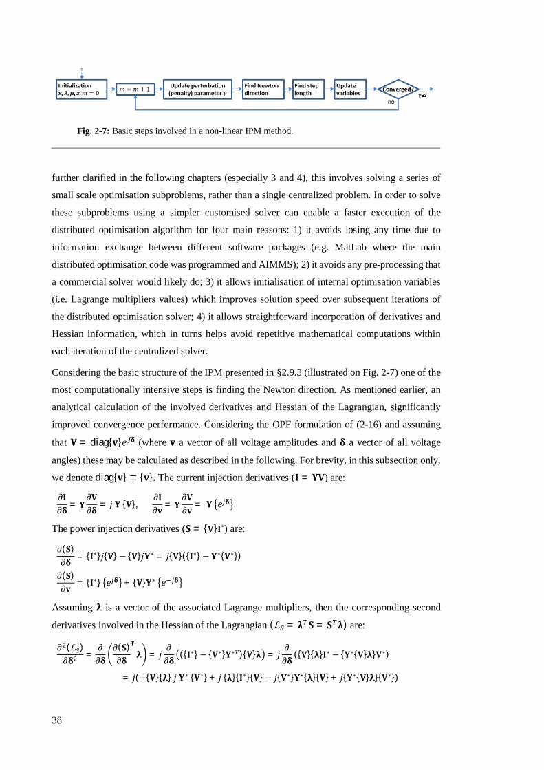
38
further clarified in the following chapters (especially 3 and 4), this involves solving a series of
small scale optimisation subproblems, rather than a single centralized problem. In order to solve
these subproblems using a simpler customised solver can enable a faster execution of the
distributed optimisation algorithm for four main reasons: 1) it avoids losing any time due to
information exchange between different software packages (e.g. MatLab where the main
distributed optimisation code was programmed and AIMMS); 2) it avoids any pre-processing that
a commercial solver would likely do; 3) it allows initialisation of internal optimisation variables
(i.e. Lagrange multipliers values) which improves solution speed over subsequent iterations of
the distributed optimisation solver; 4) it allows straightforward incorporation of derivatives and
Hessian information, which in turns helps avoid repetitive mathematical computations within
each iteration of the centralized solver.
Considering the basic structure of the IPM presented in §2.9.3 (illustrated on Fig. 2-7) one of the
most computationally intensive steps is finding the Newton direction. As mentioned earlier, an
analytical calculation of the involved derivatives and Hessian of the Lagrangian, significantly
improved convergence performance. Considering the OPF formulation of (2-16) and assuming
that 퐕 = diag{퐯}푒 훅 (where 퐯 a vector of all voltage amplitudes and 훅 a vector of all voltage
angles) these may be calculated as described in the following. For brevity, in this subsection only,
we denote diag{퐯} ≡ {퐯}. The current injection derivatives (퐈 = 퐘퐕) are:
휕퐈휕훅 = 퐘
휕퐕휕훅 = 푗 퐘 {퐕},
휕퐈휕퐯 = 퐘
휕퐕휕퐯 = 퐘 푒푗훅
The power injection derivatives (퐒 = {퐕}퐈∗) are:
휕(퐒)휕훅 = {퐈∗}푗{퐕} − {퐕}푗퐘∗ = 푗{퐕}({퐈∗} − 퐘∗{퐕∗})
휕(퐒)휕퐯 = {퐈∗} 푒푗훅 + {퐕}퐘∗ 푒−푗훅
Assuming 훌 is a vector of the associated Lagrange multipliers, then the corresponding second
derivatives involved in the Hessian of the Lagrangian (ℒ = 훌 퐒 = 퐒 훌) are:
휕 (ℒ )휕훅 =
휕휕훅
휕(퐒)휕훅
퐓
훌 = 푗휕휕훅
({퐈∗}− {퐕∗}퐘∗ ){퐕}훌 = 푗휕휕훅
({퐕}{훌}퐈∗ − {퐘∗{퐕}훌}퐕∗)
= 푗(−{퐕}{훌} 푗 퐘∗ {퐕∗} + 푗 {훌}{퐈∗}{퐕}− 푗{퐕∗}퐘∗{훌}{퐕} + 푗{퐘∗{퐕}훌}{퐕∗})
Fig. 2-7: Basic steps involved in a non-linear IPM method.

39
휕 (ℒ )휕퐯휕훅 =
휕휕퐯
휕(퐒)휕훅
퐓
훌 = 푗휕휕퐯
({퐕}{훌}퐈∗ − {퐘∗{퐕}훌}퐕∗)
= 푗 {훌}{퐈∗} 푒 훅 + {퐕}{훌}퐘∗ 푒 훅 − {퐕∗}퐘∗{훌} 푒 훅 − {퐘∗{퐕}훌} 푒 훅
휕 (ℒ )휕퐯 =
휕휕퐯
휕(퐒)휕퐯
퐓
훌 =휕휕퐯
{퐈∗} 푒 훅 + 푒 훅 퐘∗{퐕} 훌 =휕휕퐯 푒 훅 {훌}퐈∗ + 푒 훅 퐘∗푻{훌}퐕
= 푒 훅 {훌}퐘∗ 푒 훅 + 푒 훅 퐘∗{훌} 푒 훅
휕 (ℒ )휕훅휕퐯 =
휕휕훅
휕(퐒)휕퐯
퐓
훌 =휕휕훅 푒 훅 {훌}퐈∗ + 푒 훅 퐘∗{훌}퐕
= 푗 {퐈∗}{훌} 푒 훅 − 푒 훅 {훌}퐘∗{퐕∗} + 푒 훅 퐘∗{훌}{퐕}− {퐘∗{훌}퐕} 푒 훅
=휕 (ℒ )휕퐯휕훅
Regarding the line currents (퐈 = 퐘 퐕):
휕퐈휕훅 = 푗 퐘 {퐕},
휕퐈풕휕퐯 = 퐘 푒푗훅
Assuming 훍 is a vector of the associated Lagrange multipliers, then the second derivatives
involved in the Hessian of the Lagrangian ℒ = 훍 퐈 = 훍 퐈 are:
휕 ℒ퐼푡휕훅 =
휕휕훅
(푗{퐕}풀퐓훍) = −{풀퐓훍}{퐕}
휕 ℒ퐼푡휕퐯휕훅 =
휕휕퐯
(푗{퐕}풀 훍) = 푗{풀퐓훍} 푒 훅
휕 ℒ퐼푡휕퐯 =
휕휕퐯 푒푗훅 풀 훍 = 0
휕 ℒ퐼푡휕훅휕퐯 =
휕휕훅 푒푗훅 풀 훍 = 푗{풀퐓훍} 푒 훅
The derivatives associated to the remaining (linear) terms involved in the constraints are easy to
calculate, thus we do not discuss them further here.
Some convergence examples using the IPM and the analytical derivatives described above may
be seen on Fig. 2-8. Our customised solver was validated through convergence results
comparisons (in terms of optimisation decision variables and Lagrange multipliers values) with
the MatLab fmincon function, the ipopt of the MatPower package, and for base IEEE test cases
OPF problems, with a corresponding formulation in AIMMS. In all tested cases the same optimal
points were found. However, we would like to stress that in terms of convergence time, we do not
make any claim that our customised solver performs better than the others in isolated centralized
problems. After all the development of a centralized solver is beyond the scope of this work.
Nevertheless, due to the reasons discussed above, our implementation gave faster results when
applied within the distributed optimisation procedures described in Chapters 3 and 4.
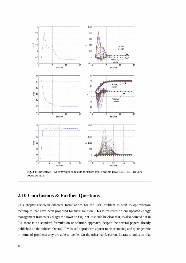
40
2.10 Conclusions & Further Questions
This chapter reviewed different formulations for the OPF problem as well as optimization
techniques that have been proposed for their solution. This is reflected on our updated energy
management framework diagram shown on Fig. 2-9. It should be clear that, as also pointed out in
[5], there is no standard formulation or solution approach, despite the several papers already
published on the subject. Overall IPM based approaches appear to be promising and quite generic
in terms of problems they are able to tackle. On the other hand, current literature indicates that
Fig. 2-8: Indicative IPM convergence results for (from top to bottom row) IEEE-24, 118, 300 nodes systems.
0 5 10 156
6.5
7
7.5
8
8.5
9
iteration
cost
0 5 10 15-200
0
200
400
600
800
1000
iteration
activepower
reactivepower
0 5 10 1512
13
14
15
16
17
18
iteration
cost
0 5 10 15-80
-60
-40
-20
0
20
40
60
iteration
reactivepower
activepower
0 5 10 15 2045
50
55
60
65
70
75
iteration
cost
0 5 10 15 20-500
0
500
1000
1500
2000
2500
iteration

41
sequential or trust-region based methods are more robust but slower compared to IPM for small
to medium scale problems. There is also a slight implication that they might be closer to what
power industry would use [95].
In terms of network constraints formulation, at the transmission level we opt to use the standard
ac formulation given that there are no clear guarantees that any of the proposed alternatives might
perform better. In terms of optimization problems centralized solution approach, we implemented
and use a basic form of the primal-dual interior point method. The reason is that it is faster than
its trust-region counterparts and given that we are interested in solving the smaller scale problems
generated through mathematical decomposition approaches it is expected to perform adequately
well. In hindsight that was the case and we did not encounter any problems with the solution of
any of our small-scale problems (i.e. those involved in the methods presented in the following
chapters). We do however revisit (in chapter 5) the sequential programming / trust-region type of
approach in the context of an OPF solution at the distribution level. The reason is that due to the
fact that networks at that level are unbalanced and the number of controls significantly large and
often discrete, the ensuing optimization problems would still be of a relatively large scale. As
Fig. 2-9: The updated energy management schematic. There is a wide variety of algorithms which could potentially solve OPF problems (Interior-Point, Trust-Region or Sequential Linear Programming). However, as the problem scale increases convergence can become more difficult or altogether fail, while for the most robust OPF approaches including distribution constraints would imply a significant increase in computational time. Note that distribution networks are not currently optimized and as such the relevant formulations and solution approaches are not yet incorporated into ED. This link will be established in a following chapter.

42
such the reliability and speed offered by the linear or quadratic subproblems formulations in
sequential programming methods is of interest. In addition, such approaches would allow us to
take advantage of the approximate linear unbalanced OPF formulation. As will be discussed in a
later chapter this can actually be an effective way to solve distribution level optimization
problems.
Closing, while the optimization algorithms discussed above could find application within the ED
problem, scalability is always an issue. It would be doubtful, even in the most basic OPF
formulation, whether convergence could be achieved in reasonable time when the constraints of
a large number of controllable loads, and both transmission and distribution level are included.
Nevertheless, it reasonable to ask whether or not it would be possible to develop specialized
highly efficient centralized solvers which could deal with this very large scale problem. However,
even if that were the case, it would presuppose that it is possible to establish a fast and reliable
communications infrastructure which could handle the communications burden of transmitting
the required information to / from that centralized solver. As such in the following we focus on
the opposite question of whether or not it would be possible to implement a decentralized solution
approach.
43
3 Decentralized Optimal Power Flow
This chapter investigates how the standard optimal power flow problem could be solved in a decentralized manner. More specifically it focuses on the balanced (transmission level) form of the problem and the following questions: 1) what are appropriate mathematical decomposition methods; 2) what is the decomposition structure (i.e. how would the original problem be divided into subproblems); 3) to what extent is decentralization possible.
3.1 Problem Statement
The basic formulation for OPF in balanced transmission systems was presented in the previous
chapter. This comes with the following starting assumptions:
A1. We consider a simplified version of the OPF problem in that contingency and reserve
constraints are not taken into account.
A2. We assume that no time-linkages exist with the future or prior states of the optimization
variables, or if any such linkages exist they may be potentially represented through terms in the
objective function.
A3. Prior to the balancing market a forward market has been cleared. Based on that, conventional
generators have set their operating status (on/off) and as such we do not deal with the associated
cost non-convexities.
A4. The problem is assumed to be solved at fixed intervals (e.g. 10-20 min) relatively close to
real-time. On one hand this implies that the solution has to be given within that interval, on the
other that all constraints and variables may be considered to be deterministic.
A5. We assume that all available controls and decisions (e.g. generation output or load
curtailments) are continuous.
A6. We do not consider distribution network constraints on the assumption that the networks
are designed in such a way that they can meet maximum demand without any problem.
3.2 Decomposition Structure
This section addresses two basic questions: a) how to determine the subsets into which the set 퐶
in (2-15) will be decomposed to (i.e. the subproblems), and b) how to perform the decomposition
assuming the desired subsets are known. Each subproblem attempts to maximize the economic
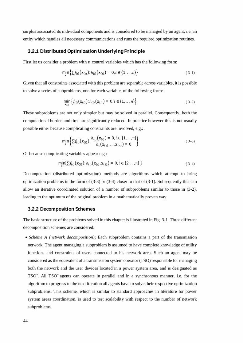
44
surplus associated its individual components and is considered to be managed by an agent, i.e. an
entity which handles all necessary communications and runs the required optimization routines.
3.2.1 Distributed Optimization Underlying Principle
First let us consider a problem with 푛 control variables which has the following form:
min퐱
∑푓{ } 퐱( ) :ℎ{ } 퐱( ) = 0, 푖 ∈ {1, … ,푛} ( 3–1)
Given that all constraints associated with this problem are separable across variables, it is possible
to solve a series of subproblems, one for each variable, of the following form:
min퐱( )
푓{ } 퐱( ) :ℎ{ } 퐱( ) = 0, 푖 ∈ {1, … , 푛} ( 3–2)
These subproblems are not only simpler but may be solved in parallel. Consequently, both the
computational burden and time are significantly reduced. In practice however this is not usually
possible either because complicating constraints are involved, e.g.:
min퐱
∑푓{ } 퐱( ) :ℎ{ } 퐱( ) = 0, 푖 ∈ {1, … ,푛}ℎ 퐱( ), … , 퐱( ) = 0
( 3–3)
Or because complicating variables appear e.g.:
min퐱
∑푓{ } 퐱( ) :ℎ{ } 퐱( ),퐱( ) = 0, 푖 ∈ {2, … , 푛} ( 3–4)
Decomposition (distributed optimization) methods are algorithms which attempt to bring
optimization problems in the form of (3-3) or (3-4) closer to that of (3-1). Subsequently this can
allow an iterative coordinated solution of a number of subproblems similar to those in (3-2),
leading to the optimum of the original problem in a mathematically proven way.
3.2.2 Decomposition Schemes
The basic structure of the problems solved in this chapter is illustrated in Fig. 3-1. Three different
decomposition schemes are considered:
Scheme A (network decomposition): Each subproblem contains a part of the transmission
network. The agent managing a subproblem is assumed to have complete knowledge of utility
functions and constraints of users connected to his network area. Such an agent may be
considered as the equivalent of a transmission system operator (TSO) responsible for managing
both the network and the user devices located in a power system area, and is designated as
TSO*. All TSO* agents can operate in parallel and in a synchronous manner, i.e. for the
algorithm to progress to the next iteration all agents have to solve their respective optimization
subproblems. This scheme, which is similar to standard approaches in literature for power
system areas coordination, is used to test scalability with respect to the number of network
subproblems.

45
Scheme B (network and user decomposition): The power system is decomposed
simultaneously to network areas and individual network user blocks. For each network area a
TSO agent manages the corresponding subset of transmission constraints (2-16) (note that in
contrast with the TSO* agents, the TSO problem no longer contains any user/device constraints
as these are now handled independently of the network). A set of network users, represented
by constraints similar to (2-19), is managed by a microgrid operator (MO). An MO agent would
in practice represent any number of nearby located users (at the extremes it could represent a
single user or all the users at a specific bus), and would have to deal with the peculiarities of
end user equipment and demands (e.g. communication issues, unexpected requests etc.). Again
all agents can work in parallel. This scheme is used to test scalability with respect to the
disaggregation of network users.
Scheme C (network and user decomposition with user aggregation): This is a two-step
decomposition scheme used to test the effects of aggregation with respect to network users.
First the initial problem is decomposed to TSO subproblems (as in scheme B) and bus
aggregator subproblems. These bus aggregators could be considered the equivalent of a
distribution system operator (DSO). Each bus aggregator subproblem (designated as DSO*)
contains the objectives and constraints of all users supplied through a specific bus. Then each
DSO* subproblem is further decomposed to individual MO subproblems and an aggregator
subproblem (designated as DSO) which effectively sums up the MO agents response, thus
limiting communications and computational requirements for TSO agents. This scheme is used
Fig.3-1: Left: A typical transmission network schematic (IEEE-24 nodes test system). The network is assumed to be separated into four control areas. Right: Tested decomposition schemes and sample illustration of generated subproblems interrelations. Each block represents a subproblem / agent and each line indicates a required bidirectional communications link.

46
to test the effects of aggregation with respect to network users. Intuitively this is also the
scheme that might be closer to what could eventually be applied in practice, as aggregators are
often thought of as a necessary part of demand management [96, 97].
These three schemes effectively represent all possible sensible decomposition structures in the
typical OPF problem. The only other possibility would be an approach akin to scheme C with
even more decomposition steps/layers. However, there does not appear to be a clear justification
for pursuing such a solution and it would no longer have any direct association with the physical
power system structure. Note that as seen on Fig.3-1 in all decomposition schemes the network
may be divided in separate areas. In case such a division is not readily available, it may be
obtained through a variety of network partitioning methods [98], such as the spectral partitioning
method discussed in the following subsections.
3.2.3 Spectral Partitioning
One approach to partitioning a graph (such as a power network) is using the so called spectral
methods. Such methods base their results on the eigenvectors of the Laplacian matrix of a graph's
connectivity matrix. For a given set of points (in our case network buses) 푥{ }, … , 푥{ } that need
to be clustered in 푘 subsets a basic spectral clustering algorithm involves the following steps [99]:
Algorithm 3-1: spectral partitioning
1. Form an 푛 × 푛 matrix 퐀 based on some distance metric whose elements indicate a
relation between given points.
2. Define the matrix 퐃 = 푑푖푎푔 ∑ 퐀( , )∈{ ,…, } , … ,∑ 퐀( , )∈{ ,…, } and calculate the
normalized Laplacian of 퐀 which is equal to 퐋 = 퐃 . 퐀퐃 . .
3. Find the eigenvalues and eigenvectors of 퐋 . Let 퐕 be a 푛푥푘 matrix derived by the
concatenation of the eigenvectors corresponding to the 푘 smallest eigenvalues.
4. Form the matrix 퐕 by normalizing each of 퐕's rows to have unit length.
5. Treating each row of 퐕 as a point in ℝ assign them into 푘 clusters using a suitable
algorithm. One of the most commonly used is the k-means algorithm described in the
following subsection.
6. Assign a point 푥{ } to cluster 푗 if row 푖 of the matrix 퐕 was assigned to cluster 푗.
In the particular case of power systems analysis the matrix 퐀 may be set to be equal to the bus
admittance matrix which effectively implies that the partitioning results become independent of
the operating state of the system. Further information may be found in [100].
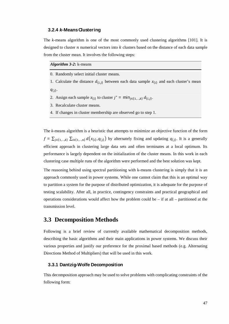
47
3.2.4 k-Means Clustering
The k-means algorithm is one of the most commonly used clustering algorithms [101]. It is
designed to cluster 푛 numerical vectors into 푘 clusters based on the distance of each data sample
from the cluster mean. It involves the following steps:
Algorithm 3-2: k-means
0. Randomly select initial cluster means.
1. Calculate the distance 푑{ , } between each data sample 푥{ } and each cluster’s mean
푞{ }.
2. Assign each sample 푥{ } to cluster 푗∗ = min ∈{ ,…, } 푑{ , }.
3. Recalculate cluster means.
4. If changes in cluster membership are observed go to step 1.
The k-means algorithm is a heuristic that attempts to minimize an objective function of the form
푓 = ∑ ∑ 푑 푥{ },푞{ }∈{ ,…, }∈{ ,…, } by alternately fixing and updating 푞{ }. It is a generally
efficient approach in clustering large data sets and often terminates at a local optimum. Its
performance is largely dependent on the initialization of the cluster means. In this work in each
clustering case multiple runs of the algorithm were performed and the best solution was kept.
The reasoning behind using spectral partitioning with k-means clustering is simply that it is an
approach commonly used in power systems. While one cannot claim that this is an optimal way
to partition a system for the purpose of distributed optimization, it is adequate for the purpose of
testing scalability. After all, in practice, contingency constraints and practical geographical and
operations considerations would affect how the problem could be – if at all – partitioned at the
transmission level.
3.3 Decomposition Methods
Following is a brief review of currently available mathematical decomposition methods,
describing the basic algorithms and their main applications in power systems. We discuss their
various properties and justify our preference for the proximal based methods (e.g. Alternating
Directions Method of Multipliers) that will be used in this work.
3.3.1 Dantzig-Wolfe Decomposition
This decomposition approach may be used to solve problems with complicating constraints of the
following form:
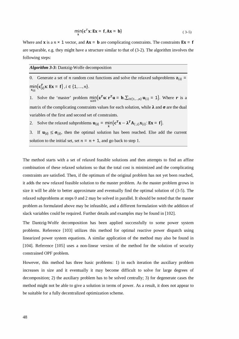
48
min퐱
{퐜 퐱:퐄퐱 = 퐟,퐀퐱 = 퐛} ( 3–5)
Where and 퐱 is a 푛 × 1 vector, and 퐀퐱 = 퐛 are complicating constraints. The constraints 퐄퐱 = 퐟
are separable, e.g. they might have a structure similar to that of (3-2). The algorithm involves the
following steps:
Algorithm 3-3: Dantzig-Wolfe decomposition
0. Generate a set of 푛 random cost functions and solve the relaxed subproblems 퐳(풊) =
min퐱{풊}
퐜{풊}푻 퐱:퐄퐱 = 퐟 , 푖 ∈ {1, … ,푛}.
1. Solve the ‘master’ problem min 퐳푻퐮: 퐫푻퐮 = 퐛,∑ 퐮( )∈{ ,…, } = 1 . Where 풓 is a
matrix of the complicating constraints values for each solution, while 훌 and 훔 are the dual
variables of the first and second set of constraints.
2. Solve the relaxed subproblems 퐮{풊} = min퐱
퐜푻퐱 − 훌휯퐀(:, )퐱{ }: 퐄퐱 = 퐟 .
3. If 퐮{풊} ≤ 훔{풊}, then the optimal solution has been reached. Else add the current
solution to the initial set, set 푛 = 푛 + 1, and go back to step 1.
The method starts with a set of relaxed feasible solutions and then attempts to find an affine
combination of these relaxed solutions so that the total cost is minimized and the complicating
constraints are satisfied. Then, if the optimum of the original problem has not yet been reached,
it adds the new relaxed feasible solution to the master problem. As the master problem grows in
size it will be able to better approximate and eventually find the optimal solution of (3-5). The
relaxed subproblems at steps 0 and 2 may be solved in parallel. It should be noted that the master
problem as formulated above may be infeasible, and a different formulation with the addition of
slack variables could be required. Further details and examples may be found in [102].
The Dantzig-Wolfe decomposition has been applied successfully to some power system
problems. Reference [103] utilizes this method for optimal reactive power dispatch using
linearized power system equations. A similar application of the method may also be found in
[104]. Reference [105] uses a non-linear version of the method for the solution of security
constrained OPF problem.
However, this method has three basic problems: 1) in each iteration the auxiliary problem
increases in size and it eventually it may become difficult to solve for large degrees of
decomposition; 2) the auxiliary problem has to be solved centrally; 3) for degenerate cases the
method might not be able to give a solution in terms of power. As a result, it does not appear to
be suitable for a fully decentralized optimization scheme.
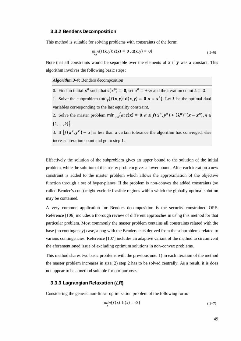
49
3.3.2 Benders Decomposition
This method is suitable for solving problems with constraints of the form:
푚푖푛퐱,퐲
{푓(퐱, 퐲):퐜(퐱) = ퟎ ,퐝(퐱,퐲) = ퟎ} ( 3–6)
Note that all constraints would be separable over the elements of 퐱 if 퐲 was a constant. This
algorithm involves the following basic steps:
Algorithm 3-4: Benders decomposition
0. Find an initial 퐱 such that 퐜(퐱 ) = ퟎ, set 푎 = +∞ and the iteration count 푘 = 0.
1. Solve the subproblem min퐲{푓(퐱, 퐲):퐝(퐱, 퐲) = ퟎ,퐱 = 퐱 }. Let 훌 be the optimal dual
variables corresponding to the last equality constraint.
2. Solve the master problem min ,퐱 훼: 퐜(퐱) = ퟎ,훼 ≥ 풇(풙 ,풚 ) + (훌 ) (풙 − 풙 ),푛 ∈
{1, … ,푘} .
3. If 푓 퐱 , 퐲 − 훼 is less than a certain tolerance the algorithm has converged, else
increase iteration count and go to step 1.
Effectively the solution of the subproblem gives an upper bound to the solution of the initial
problem, while the solution of the master problem gives a lower bound. After each iteration a new
constraint is added to the master problem which allows the approximation of the objective
function through a set of hyper-planes. If the problem is non-convex the added constraints (so
called Bender’s cuts) might exclude feasible regions within which the globally optimal solution
may be contained.
A very common application for Benders decomposition is the security constrained OPF.
Reference [106] includes a thorough review of different approaches in using this method for that
particular problem. Most commonly the master problem contains all constraints related with the
base (no contingency) case, along with the Benders cuts derived from the subproblems related to
various contingencies. Reference [107] includes an adaptive variant of the method to circumvent
the aforementioned issue of excluding optimum solutions in non-convex problems.
This method shares two basic problems with the previous one: 1) in each iteration of the method
the master problem increases in size; 2) step 2 has to be solved centrally. As a result, it is does
not appear to be a method suitable for our purposes.
3.3.3 Lagrangian Relaxation (LR)
Considering the generic non-linear optimization problem of the following form:
푚푖푛퐱
{푓(퐱):퐡(퐱) = ퟎ } ( 3–7)
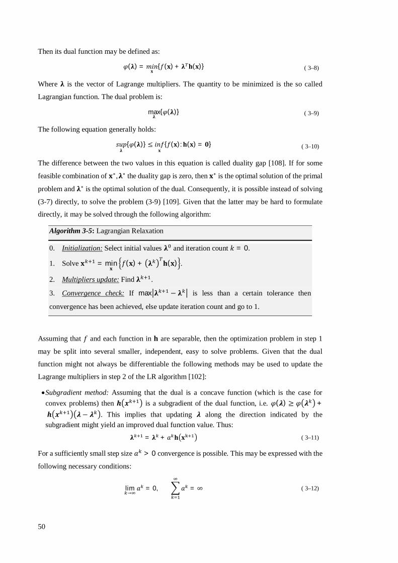
50
Then its dual function may be defined as:
휑(훌) = 푚푖푛퐱
{푓(퐱) + 훌 퐡(퐱)} ( 3–8)
Where 훌 is the vector of Lagrange multipliers. The quantity to be minimized is the so called
Lagrangian function. The dual problem is:
max훌
{휑(훌)} ( 3–9)
The following equation generally holds:
푠푢푝훌
{휑(훌)} ≤ 푖푛푓퐱
{푓(퐱):퐡(퐱) = ퟎ} ( 3–10)
The difference between the two values in this equation is called duality gap [108]. If for some
feasible combination of 퐱∗,훌∗ the duality gap is zero, then 퐱∗ is the optimal solution of the primal
problem and 훌∗ is the optimal solution of the dual. Consequently, it is possible instead of solving
(3-7) directly, to solve the problem (3-9) [109]. Given that the latter may be hard to formulate
directly, it may be solved through the following algorithm:
Algorithm 3-5: Lagrangian Relaxation
0. Initialization: Select initial values 훌 and iteration count 푘 = 0.
1. Solve 퐱 = min퐱
푓(퐱) + 훌 퐡(퐱) .
2. Multipliers update: Find 훌 .
3. Convergence check: If max 훌 − 훌 is less than a certain tolerance then
convergence has been achieved, else update iteration count and go to 1.
Assuming that 푓 and each function in 퐡 are separable, then the optimization problem in step 1
may be split into several smaller, independent, easy to solve problems. Given that the dual
function might not always be differentiable the following methods may be used to update the
Lagrange multipliers in step 2 of the LR algorithm [102]:
Subgradient method: Assuming that the dual is a concave function (which is the case for convex problems) then 풉 풙 is a subgradient of the dual function, i.e. 휑(흀) ≥ 휑 흀 + 풉 풙 흀− 흀 . This implies that updating 흀 along the direction indicated by the subgradient might yield an improved dual function value. Thus:
훌 = 훌 + 푎 퐡 퐱 ( 3–11)
For a sufficiently small step size 푎 > 0 convergence is possible. This may be expressed with the
following necessary conditions:
lim→
푎 = 0, 푎 = ∞ ( 3–12)
51
Intuitively (3-12) implies that while 푎 should decrease as the iteration count increases, it should
never become zero. In that case, it follows from (3-11) that the Lagrange multipliers would not
be updated and the algorithm would stop prematurely. While this method is very simple to
implement, a standard approach for setting the step size does not seem to be available. At the
same time the selection of this parameter can have a significant impact on convergence.
Cutting Plane method: In order to determine multiplier updates this approach requires the solution of the following optimization subproblem:
max,흀
푧: 푧 ≤ 휑(훌 ) + 퐡(풙 ) (훌− 훌 ), 푖 ∈ {1, … ,푘} ( 3–13)
This approach essentially attempts to reconstruct the dual function using a set of subgradients.
While it can lead to faster convergence compared to the subgradient method, the size of the
optimization problem increases significantly with the number of iterations. In addition, the
problem (3-13) requires to be centrally solved, and as such it does not easily allow for fully
decentralized solutions.
Bundle method: This method involves solving (3-13) with an additional penalty term in the
objective function of the form 푎 흀 − 휣 , where 휣 is the so called centre of gravity which
has to be suitably updated in every iteration. The method is a variant of the cutting plane
approach but it requires careful tuning of the additional parameters in order to be efficient.
Trust region method: This is another variant of the cutting plane method. Its basic difference
is that it uses only a limited set of the closest hyper-planes to the solution of interest and as a
result the problem size remains constant. Bounds on the values of Lagrange multipliers may be
dynamically updated. Again the decomposability of the relevant problem is an issue.
Overall, possibly due to its simplicity, LR has been a quite popular method in power systems. In
[110] LR with a subgradient based update is used to solve a simplified unit commitment problem.
Only a global power balance constraint is considered and commitment problems of individual
units are solved using dynamic programming. The paper also illustrates the inability of
subgradient based LR to converge when similar units exist in the system. In such cases the price
(i.e. Lagrange multiplier) signal given through this decomposition approach is not adequate. As a
result, the use of a heuristic by the system operator would be necessary, but then the optimality
of the solution would be in question. For example, in [111] a few simple rules are combined with
the standard LR approach for the solution of the unit commitment problem: a) The start-up cost
normalized by the number of operating hours is added to the hourly variable cost to determine
whether or not a unit turns on. This is used instead of dynamic programming. b) Depending on
their type certain units (e.g. base units) are ignored by the heuristic. c) Units with similar
characteristics are committed as a group and then decommitted one by one as long as demand and
reserve requirements are satisfied. d) Committed units are sorted in terms of cost and are turned
off or substituted by other units by checking each in turn. A similar approach is followed in [112]

52
where a variety of empirical rules are used for updating the Lagrange multipliers depending on
whether or not reserve and active power balance constraints are satisfied. It should be clear
however that heuristics such as this require centralized control.
Reference [113] discusses the formulation of LR subproblems when reserve constraints are
included in the initial OPF, based on DC equations. The algorithm is tested on a simple 6 unit
system. Reference [114] uses the LR approach with a subgradient method for the decomposition
of an OPF problem, which is separated into three subproblems. Each subproblem / area is a copy
of the IEEE RTS. The method is shown to converge within a few tens of iterations to accurate
results. However, this may not be necessarily expected for the general case. The good
convergence might mostly have to do with the fact that the tie-line flows between areas did not
have a significant effect on the system Lagrange multiplier values.
Reference [115] focuses in solving the dual of a relaxed mixed-integer unit commitment problem.
The transmission system is not explicitly modelled and only two constraints, regarding reserve
requirements and global power balance, are included. The method used is LR with a trust region
based update of multipliers and indicates improved convergence compared to other updating
techniques.
In [116] the full AC single period optimal power flow is solved. A 5 bus system is used and
decomposition to the individual generator / demand block is performed. The transmission system
problem is solved as a single problem. Convergence is achieved in less than 20 iterations. A
central entity is responsible for the exchange of Lagrange multiplier information. It uses a Newton
method to update the associated Lagrange multipliers. The required derivatives for the Newton
step can be calculated based on market players’ previous responses.
In [117] the LR is coupled with cutting plane methods for multiplier updates. Tests are carried
out in a 6 bus system including a number of 4000 network user subproblems. Two different
cutting plane approaches are compared in terms of convergence performance.
Reference [118] uses an LR scheme with a subgradient method to solve a power system demand
management problem. The paper recognizes the inefficiency of this approach’s convergence in
non-strongly-convex problems. It proposes a simple heuristic which limits the maximum power
consumption per hour for individual consumers. While this problem might solve the issue of
demand allocation in the forward market (as long as the demand involves continuous functions),
it is not clear how it affects the generators commitment problem. Furthermore, the overall
optimization problem has to be solved for a variety of limit values and the optimal solution has
to be selected among them. This is bound to increase the computational burden, and brings up the
question of how to determine this set of limit values. The second part of this work [119] applies
the method in a test case based on the UK system, including electric vehicles and thermal loads.
Transmission constraints are not considered however and the reported low numbers of iterations

53
to convergence might be misleading given that the multipliers initial values appear to be set very
close to the actual solution. Finally, in [120] a quite similar approach is used including DC power
flow equations. The test system is a 16 bus representation of the UK network. No results on the
number of iterations to convergence are reported.
In [121] a decentralized trading scheme based on LR is proposed. The authors recognize the fact
that due to the generators’ cost non-convexities a market equilibrium might not exist. The
proposed solution is the force the so called ‘convexifying market rule’ to surpass this problem. A
market is said to operate under this rule as long as the trial price – response pairs may be extended
to a monotone incremental cost (or monotone decreasing incremental benefit) function. How
actually a market clearing strategy using this rule would work however is not clarified.
Overall, LR yields simple easily coordinated subproblems. However, there are three issues with
this method: 1) in its basic form with subgradient multiplier updates it has poor convergence
performance if the subproblem objective functions are not strongly convex (an example may be
seen on Fig. 3-2); 2) in any of its improved forms degenerate solutions can be an issue as even if
Lagrange multipliers converge, power might not; 3) improved methods for Lagrange multiplier
updates typically imply centralized solutions of the Lagrange multiplier update problem. As a
consequence, LR does not fully satisfy our requirements for a decentralized solution method.
The convergence issues identified above (also illustrated with a simpler example in [122]) may
be resolved by considering an augmented form of the Lagrangian, i.e.:
ℒ (퐱,훌) = 푓(퐱) + 훌 퐡(퐱) +휌2‖퐡(퐱)‖ ( 3–14)
Where 휌 is a penalty factor, which should be sufficiently small so that the problem does not
become ill conditioned [109, 123]. At the optimal point the last term is equal to zero and as a
result has no impact on the final solution of the problem. However, it makes the problem strongly
convex (at least in a region around the optimum) with respect to x and due to this fact offers
improved convergence. The disadvantage of the augmented Lagrangian is that (3-14) is no longer
Fig. 3-2: Simple example illustrating the performance of LR in IEEE-24 test system (split into three areas) with subgradient updates of Lagrange multipliers. This oscillatory behaviour is rather typical of the method and careful tuning would be required to achieve acceptable convergence results.
0 100 200 300 400 500-20
0
20
40
60
iteration
LMP
(£/M
Wh)
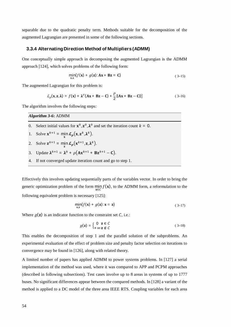
54
separable due to the quadratic penalty term. Methods suitable for the decomposition of the
augmented Lagrangian are presented in some of the following sections.
3.3.4 Alternating Direction Method of Multipliers (ADMM)
One conceptually simple approach in decomposing the augmented Lagrangian is the ADMM
approach [124], which solves problems of the following form:
min퐱,퐳
{푓(퐱) + 푔(퐳):퐀퐱+ 퐁퐳 = 퐂} ( 3–15)
The augmented Lagrangian for this problem is:
ℒ (퐱, 퐳,훌) = 푓(퐱) + 훌 (퐀퐱+ 퐁퐳− 퐂) +휌2‖퐀퐱 + 퐁퐳 − 퐂‖ ( 3–16)
The algorithm involves the following steps:
Algorithm 3-6: ADMM
0. Select initial values for 퐱 , 퐳 ,훌 and set the iteration count 푘 = 0.
1. Solve 퐱 = min퐱퓛흆 퐱, 퐳 ,훌 .
2. Solve 퐳 = min퐳퓛흆 퐱 , 퐳,훌 .
3. Update 훌 = 훌 + 휌 퐀퐱 + 퐁퐳 − 퐂 .
4. If not converged update iteration count and go to step 1.
Effectively this involves updating sequentially parts of the variables vector. In order to bring the
generic optimization problem of the form min퐱∈
푓(퐱), to the ADMM form, a reformulation to the
following equivalent problem is necessary [125]:
min퐱,퐳
{푓(퐱) + 푔(퐳): 퐱 = 퐳} ( 3–17)
Where 푔(퐳) is an indicator function to the constraint set 퐶, i.e.:
푔(퐳) = 0+∞
퐳 ∈ 퐶퐳 ∉ 퐶 ( 3–18)
This enables the decomposition of step 1 and the parallel solution of the subproblems. An
experimental evaluation of the effect of problem size and penalty factor selection on iterations to
convergence may be found in [126], along with related theory.
A limited number of papers has applied ADMM to power systems problems. In [127] a serial
implementation of the method was used, where it was compared to APP and PCPM approaches
(described in following subsections). Test cases involve up to 8 areas in systems of up to 1777
buses. No significant differences appear between the compared methods. In [128] a variant of the
method is applied to a DC model of the three area IEEE RTS. Coupling variables for each area

55
subproblem are fixed to the value of their previous iteration, instead of performing the
minimization of step 2. A mathematical proof of convergence in this case is not provided however.
Another application of the method may be found in [129] where the initial problem is decomposed
down to the individual component level. Tests are carried out in randomly generated networks of
up to 3 ∙ 10 buses. The scaling results indicated by the authors look impressive, however
Kirchhoff’s laws are not taken into account. Reference [130] uses the ADMM method for the
decomposition of a semi-definite formulation of the unbalanced OPF problem in distribution
networks. For a 37 node network partitioned in 4 areas, convergence is shown to be achieved in
about 100 iterations.
In the case of the ADMM method the initial OPF problem takes the form:
min퐳,퐔∈
{푓 (퐏,퐐) + 푔(퐳): 퐳 = 퐔 } ( 3–19)
Where 푔 is an indicator function to the linear coupling constraints set 퐶 of equation (2-20) and
퐔 a vector of variables involved in 퐶 . The augmented Lagrangian becomes then equal to:
ℒ (퐔,퐳,훌 ) = 푓 (퐔) + 푔(퐳) + 훌 (퐔 − 퐳) +휌2‖퐔 − 퐳‖ ( 3–20)
The ADMM equations then become:
퐔 = argmin퐔∈ /
푓 (퐔) + (훌 ) 퐔 +휌2‖퐔 − 퐳 ‖ ( 3–21)
퐳 = Π {퐔 − 퐳} ( 3–22)
훌 = 훌 + 휌(퐔 − 퐳 ) ( 3–23)
Where Π is the Euclidian projection on the set 퐶 . These equations presuppose that the initial
values for the Lagrange multipliers are selected so that (훌 ) 퐳 = 0 ∀ {퐳 :퐡 퐳 = 0}. For
example, let us consider the constraint 푃 + 푃 = 0 and corresponding auxiliary variables
퐳( ), 퐳( ). Let 훌 ( ),훌 ( ) be the Lagrange multipliers corresponding to the constraints 퐳( ) =
푃 , 퐳( ) = 푃 and assume their initial values are selected so that 훌 ( ) = 훌 ( ). It follows from
(3-21) that 퐳( ) = −퐳( ) = 푧 and also:
푧 = min 훌 ( )푧 − 훌 ( )푧 + (푃 − 푧) + (푃 + 푧) ⇒
⇒ (푃 − 푧 ) − (푃 + 푧 ) = 0 → 푧 = (푃 − 푃 ) 2⁄ ( 3–24)
From (3-22) we then have:
훌 ( ) = 훌 ( ) + 휌(푃 − (푃 − 푃 ) 2⁄ ) = 훌 ( ) + 휌 (푃 + 푃 ) 2⁄
훌 ( ) = 훌 ( ) + 휌(푃 + (푃 − 푃 ) 2⁄ ) = 훌 ( ) + 휌 (푃 + 푃 ) 2⁄ ( 3–25)
Consequently 훌 ( ) = 훌 ( ). This result is valid for any duplicated variable. Thus for any iteration
훌 퐳 = 0. Note that the optimization subproblems and multiplier update steps are fully

56
decomposable, with the only requirement being the exchange of information between the
subproblems which are coupled by this constraint.
According to [125] necessary and sufficient conditions for convergence are primal and dual
feasibility, i.e. 퐫 = 퐳 − 퐔 = 0 and ∇푓 + 훌 퐔 = 0, with the quantity 퐬 = 휌 퐳 − 퐳
being indicative of the latter. Thus a typical requirement for convergence could be 퐫 ≤ 휖
and 퐬 ≤ 휖 , where 휖 , 휖 positive tolerance values (e.g. on the order of 10 ). Typically,
the primal residual equation would correspond to power and voltage variables equalities and
directly relates to the updates in Lagrange multipliers themselves. In a typical OPF problem if the
multipliers do not significantly vary from one iteration to the next, the change in 퐳 may also be
expected to be small and in most cases checking the primal residuals might be adequate.
3.3.5 Predictor Corrector Proximal Multipliers Method (PCPM)
The ADMM method is actually a member of one larger family of decomposition methods who
are based on the so called proximal method of multipliers [131, 13]. The latter instead of directly
solving the generic optimization problem min퐱∈
푓(퐱), reaches the solution through the iterative
process:
퐱 = min퐱∈
푓(퐱) +1
2푐‖퐱 − 퐱 ‖ ( 3–26)
The LR method may be applied to this problem [132] to enable a parallelizable solution. The
penalty term if sufficiently large (i.e. 푐 is sufficiently small) will effectively limit how much 퐱
changes over subsequent iterations. This should help achieve smooth convergence (i.e. limit
Lagrange multipliers oscillations over subsequent iterations) and resolve any degeneracy issues
(i.e. even for linear objective functions there will be a unique solution for subproblems as a
function of price or Lagrange multiplier value). A variant of this method appears in [133] where
the PCPM algorithm is presented. The method solves problems similar to (3-15) with a modified
objective function as in (3-25), and involves the following steps:
Algorithm 3-7: PCPM
0. Select initial values for 퐱 , 퐳 ,훌 and set the iteration count 푘 = 0.
1. Update predictors 퐩 = 훌 + 휌 퐀퐱 − 퐁퐳 .
2. Solve 퐱 = min퐱퓛흆 퐱, 퐳 ,퐩 .
3. Solve 퐳풌 ퟏ = min퐳퓛흆 퐱 , 퐳,퐩 .
4. Update 훌 = 훌 + 휌 퐀퐱 − 퐁퐳 .
5. If variables values do not significantly change, convergence is achieved. Otherwise
go back to step 2.
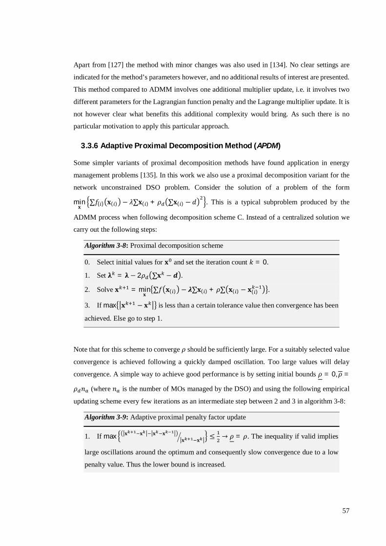
57
Apart from [127] the method with minor changes was also used in [134]. No clear settings are
indicated for the method’s parameters however, and no additional results of interest are presented.
This method compared to ADMM involves one additional multiplier update, i.e. it involves two
different parameters for the Lagrangian function penalty and the Lagrange multiplier update. It is
not however clear what benefits this additional complexity would bring. As such there is no
particular motivation to apply this particular approach.
3.3.6 Adaptive Proximal Decomposition Method (APDM)
Some simpler variants of proximal decomposition methods have found application in energy
management problems [135]. In this work we also use a proximal decomposition variant for the
network unconstrained DSO problem. Consider the solution of a problem of the form
min퐱
∑푓{ } 퐱( ) − 휆∑퐱( ) + 휌 ∑퐱( ) − 푑 . This is a typical subproblem produced by the
ADMM process when following decomposition scheme C. Instead of a centralized solution we
carry out the following steps:
Algorithm 3-8: Proximal decomposition scheme
0. Select initial values for 퐱 and set the iteration count 푘 = 0.
1. Set 훌 = 훌 − 2휌 ∑퐱 − 풅 .
2. Solve 퐱 = min퐱
∑푓 퐱( ) − 흀∑퐱( ) + 휌∑ 퐱( ) − 퐱( ) .
3. If max 퐱 − 퐱 is less than a certain tolerance value then convergence has been
achieved. Else go to step 1.
Note that for this scheme to converge 휌 should be sufficiently large. For a suitably selected value
convergence is achieved following a quickly damped oscillation. Too large values will delay
convergence. A simple way to achieve good performance is by setting initial bounds 휌 = 0,휌 =
휌 푛 (where 푛 is the number of MOs managed by the DSO) and using the following empirical
updating scheme every few iterations as an intermediate step between 2 and 3 in algorithm 3-8:
Algorithm 3-9: Adaptive proximal penalty factor update
1. If max 퐱 퐱 퐱 퐱퐱 퐱 ≤ → 휌 = 휌. The inequality if valid implies
large oscillations around the optimum and consequently slow convergence due to a low
penalty value. Thus the lower bound is increased.
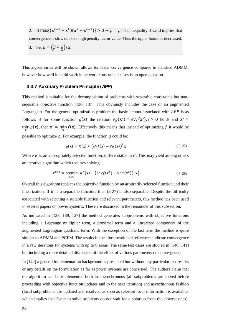
58
2. If max 퐱 − 퐱 퐱 − 퐱 ≥ 0 → 휌 = 휌. The inequality if valid implies that
convergence is slow due to a high penalty factor value. Thus the upper bound is decreased.
3. Set 휌 = 휌 + 휌 /2.
This algorithm as will be shown allows for faster convergence compared to standard ADMM,
however how well it could work in network constrained cases is an open question.
3.3.7 Auxiliary Problem Principle (APP)
This method is suitable for the decomposition of problems with separable constraints but non-
separable objective function [136, 137]. This obviously includes the case of an augmented
Lagrangian. For the generic optimization problem the basic lemma associated with 퐴푃푃 is as
follows: if for some function 푔(퐱) the relation ∇푔(퐱∗) = 휖∇푓(퐱∗), 휖 > 0 holds and 퐱∗ =
min퐱푔(퐱), then 퐱∗ = min
퐱푓(퐱). Effectively this means that instead of optimizing 푓 it would be
possible to optimize 푔. For example, the function 푔 could be:
푔(퐱) = 퐾(퐱) + 휖∇푓(퐱) − ∇퐾(퐱) 퐱 ( 3–27)
Where 퐾 is an appropriately selected function, differentiable in 퐶. This may yield among others
an iterative algorithm which requires solving:
퐱 = argmin풙∈
퐾 (퐱) + 휖 ∇푓(퐱 )− ∇퐾 (퐱 ) 퐱 ( 3–28)
Overall this algorithm replaces the objective function by an arbitrarily selected function and their
linearization. If 퐾 is a separable function, then (3-27) is also separable. Despite the difficulty
associated with selecting a suitable function and relevant parameters, this method has been used
in several papers on power systems. These are discussed in the remainder of this subsection.
As indicated in [138, 139, 127] the method generates subproblems with objective functions
including a Lagrange multiplier term, a proximal term and a linearized component of the
augmented Lagrangian quadratic term. With the exception of the last term the method is quite
similar to ADMM and PCPM. The results in the aforementioned references indicate convergence
in a few iterations for systems with up to 8 areas. The same test cases are studied in [140, 141]
but including a more detailed discussion of the effect of various parameters on convergence.
In [142] a general implementation background is presented but without any particular test results
or any details on the formulation as far as power systems are concerned. The authors claim that
the algorithm can be implemented both in a synchronous (all subproblems are solved before
proceeding with objective function updates and to the next iteration) and asynchronous fashion
(local subproblems are updated and resolved as soon as relevant local information is available,
which implies that faster to solve problems do not wait for a solution from the slowest ones).
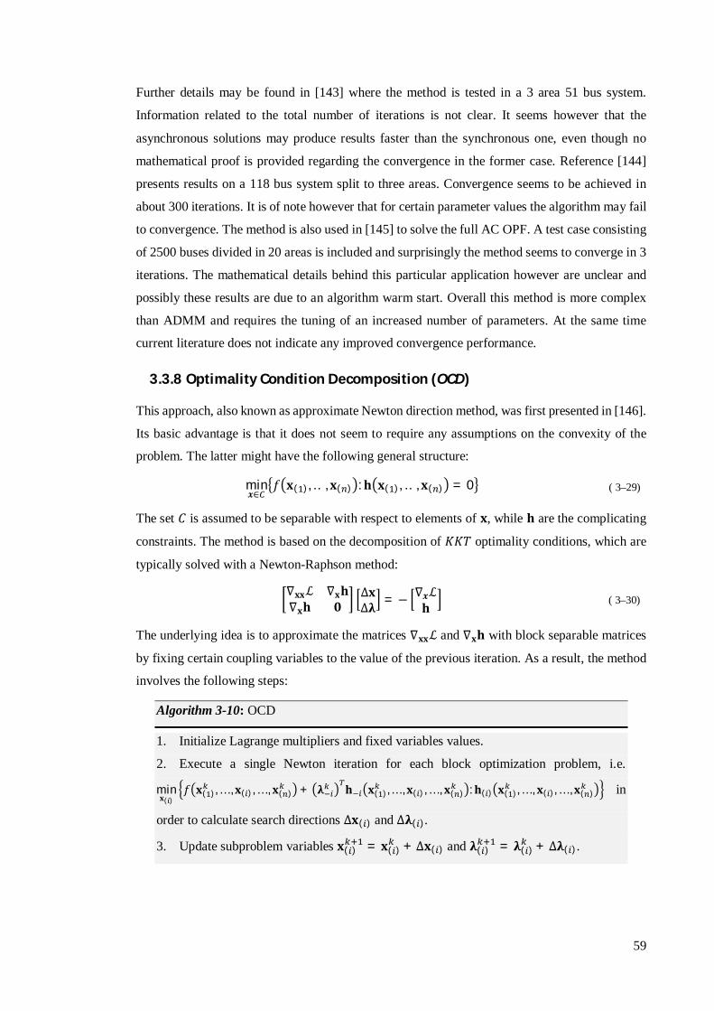
59
Further details may be found in [143] where the method is tested in a 3 area 51 bus system.
Information related to the total number of iterations is not clear. It seems however that the
asynchronous solutions may produce results faster than the synchronous one, even though no
mathematical proof is provided regarding the convergence in the former case. Reference [144]
presents results on a 118 bus system split to three areas. Convergence seems to be achieved in
about 300 iterations. It is of note however that for certain parameter values the algorithm may fail
to convergence. The method is also used in [145] to solve the full AC OPF. A test case consisting
of 2500 buses divided in 20 areas is included and surprisingly the method seems to converge in 3
iterations. The mathematical details behind this particular application however are unclear and
possibly these results are due to an algorithm warm start. Overall this method is more complex
than ADMM and requires the tuning of an increased number of parameters. At the same time
current literature does not indicate any improved convergence performance.
3.3.8 Optimality Condition Decomposition (OCD)
This approach, also known as approximate Newton direction method, was first presented in [146].
Its basic advantage is that it does not seem to require any assumptions on the convexity of the
problem. The latter might have the following general structure:
min풙∈
푓 퐱( ), … , 퐱( ) :퐡 퐱( ), … , 퐱( ) = 0 ( 3–29)
The set 퐶 is assumed to be separable with respect to elements of 퐱, while 퐡 are the complicating
constraints. The method is based on the decomposition of 퐾퐾푇 optimality conditions, which are
typically solved with a Newton-Raphson method:
∇퐱퐱ℒ ∇퐱퐡∇퐱퐡 ퟎ
Δ퐱Δ훌 = − ∇풙ℒ
퐡 ( 3–30)
The underlying idea is to approximate the matrices ∇퐱퐱ℒ and ∇퐱퐡 with block separable matrices
by fixing certain coupling variables to the value of the previous iteration. As a result, the method
involves the following steps:
Algorithm 3-10: OCD
1. Initialize Lagrange multipliers and fixed variables values.
2. Execute a single Newton iteration for each block optimization problem, i.e.
min퐱( )
푓 퐱( ), … ,퐱( ) , … , 퐱( ) + 훌 퐡 퐱( ), … ,퐱( ) , … , 퐱( ) :퐡( ) 퐱( ), … , 퐱( ), … ,퐱( ) in
order to calculate search directions Δ퐱( ) and Δ훌( ).
3. Update subproblem variables 퐱( ) = 퐱( ) + Δ퐱( ) and 훌( ) = 훌( ) + Δ훌( ).

60
4. If the variables variation over a number of consecutive iterations is less than a
specified tolerance, then the algorithm has converged. Otherwise increase iteration count
and go to step 1.
The individual optimization subproblems may also be solved to optimality [147]. One basic issue
is that due to the fixed variables these subproblems may be infeasible. Consequently, a barrier
method should be used to solve them. Furthermore, for the algorithm to converge, the solution of
(3-29) should be well defined, and if 퐊 the actual Jacobian and 퐊 its block separable
approximation then 휌 퐈 − 퐊 퐊 ≤ 1. Where 휌 denotes the spectral radius of the corresponding
matrix. In case this condition does not hold then some preconditioning method may be used,
which should adjust the variables and multiplier updates to suitable values.
The OCD method has been successfully applied in power systems multi-area OPF. In [148] the
method is applied to a variety of test systems of up to 708 systems, separated in up to 6 areas. The
algorithm is shown to converge within a few tens of iterations.
Reference [149] combines this approach with DC load flow equations, carrying out tests in
systems of up to 6 areas. In [150] further discusses some implementation considerations of this
approach. Finally, [151] extends the method to full AC equations. Convergence seems to be
achieved in a few tens of iterations, however the significant effect of tolerance values used to
check convergence is also illustrated.
In [152] the OCD method is extended and applied in a power system decomposed to several
overlapping areas. The latter are selected independently of each other based on the control effects
of various FACTS devices (i.e. power electronics based devices that enhance system
controllability). This particular extension however does not seem to hold any interest for
electricity markets.
Results in [153] seem to indicate faster convergence for this method compared to LR based
approaches for small degrees of decomposition. A technique for improving the convergence of
the latter is presented, based on a master-slave principle, but no mathematical proof of
convergence is provided. Finally, [154] proposes an asynchronous implementation of the OCD
method applied to DC equations. The method is tested in the three area IEEE RTS system, and is
shown to converge faster than the synchronous implementation.
Despite the potentially better performance of OCD compared to dual decomposition techniques
this method does not appear to be such a good candidate for decentralized OPF solutions.
Evaluating whether or not the convergence criterion holds, and performing the required
preconditioning, might not be easy in a decentralized context. Furthermore, its convergence speed
for large degrees of decomposition would also need to be investigated.
61
3.3.9 Other Approaches
One popular term used often in power system papers is that of multi-agent systems. This is not
unexpected given the rather loose definition of what an agent can be, i.e. a computer system
situated in some environment that is capable of autonomous action to meet its design objectives
[155]. As a matter of fact, the distributed optimization methods presented above may be
considered the basis of a multi-agent system, where an agent is associated with each subproblem.
However, more often than not, papers which emphasize the multi-agent systems aspects do so in
order to lend further theoretical foundations to their proposed heuristic solutions.
As an indicative example, reference [156] proposes an agent based system with a set of heuristic
rules for load balancing in the system, which is implemented in JADE (a Java based programming
framework for the development of agent-based applications). The proposed set of rules is
applicable on radial networks and involves selection of generation sources or demand to shed
based on a priority list. While the presented results indicate fast solution times, there are no
guarantees with regards to the optimality of the solution, and communications delays do not seem
to have been taken into account.
Another approach is proposed in [157] where a max-sum based algorithm is used to optimize
generation in a micro grid. A simplified DC network representation is used and the objective is
minimization of emission costs. It should be noted however that the proposed algorithm has
proven convergence only on radial networks and thus is not suitable for distributed OPF.
Reference [158] uses a consensus-based information discovery approach to determine power
imbalance in the system, information which is utilized for determining load shedding. This
concept may be easily extended to estimate a market clearing price. Such an extension is detailed
in [159] and for a 14 bus test system its results are compared to a standard subgradient LR method.
Though both approaches converge at the same optimal solution, there do not seem to be
significant benefits in the consensus method. Furthermore, it does not seem to allow the inclusion
of network constraints.
A different approach based on bi-level programming is proposed in [160]. At the higher level the
transmission system including an approximate representation of electric vehicle / demand
aggregators is optimized. At the lower level, each individual aggregator solves an optimization
problem that determines individual vehicle schedules while including a penalty for deviations
from the higher level optimization problem solution. It should be noted that this is not exactly a
full decomposition method, as the higher level problem includes some representation of the lower
level problem. In addition, performance of the method in terms of both optimality and speed is
dependent on the method’s parameters.

62
3.4 Results and Discussion
The method of choice in this work is ADMM. For each of the proposed decomposition schemes
an algorithmic flowchart may be seen on Fig. 3-3. ADMM was preferred over other augmented
Lagrangian based methods due to the fact that only a single parameter requires tuning, and yields
a relatively simple, easily decomposable multiplier update step. It was also preferred over the
OCD approach due to the fact that the latter is based on an approximation of the Jacobian derived
from KKT conditions and may require appropriate preconditioning to ensure convergence. This
is especially important in large degrees of decomposition (e.g. down to the individual device or
node level) where the approximation is much coarser. Checking whether the necessary
Fig. 3-3: Flowcharts for the decentralized solution for each of the decomposition schemes and indicative illustration of information exchange between different types of agents within a single iteration. Initialization would typically use the values of 훌, 퐳 of the last algorithm run. Regarding the information exchanges the iteration count is passed in order to facilitate agent synchronization. For purposes of error checking 훌 values could also be periodically transmitted. It should be noted that all schemes use synchronous implementation of the methods where at each iteration all subproblems have to be solved and relevant information collected, before progressing to the next. Note that schemes A and B use only ADMM. Scheme C uses ADMM at the transmission level, and the APDM method for the DSO subproblems.
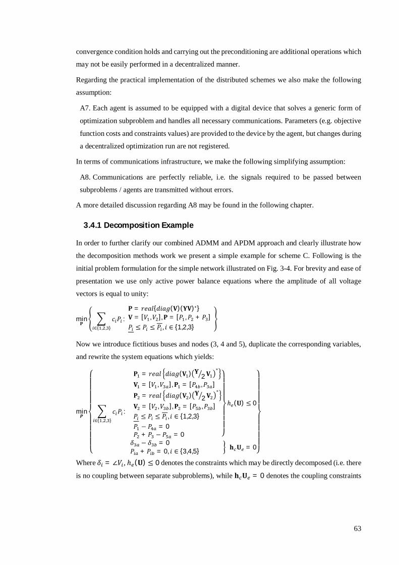
63
convergence condition holds and carrying out the preconditioning are additional operations which
may not be easily performed in a decentralized manner.
Regarding the practical implementation of the distributed schemes we also make the following
assumption:
A7. Each agent is assumed to be equipped with a digital device that solves a generic form of
optimization subproblem and handles all necessary communications. Parameters (e.g. objective
function costs and constraints values) are provided to the device by the agent, but changes during
a decentralized optimization run are not registered.
In terms of communications infrastructure, we make the following simplifying assumption:
A8. Communications are perfectly reliable, i.e. the signals required to be passed between
subproblems / agents are transmitted without errors.
A more detailed discussion regarding A8 may be found in the following chapter.
3.4.1 Decomposition Example
In order to further clarify our combined ADMM and APDM approach and clearly illustrate how
the decomposition methods work we present a simple example for scheme C. Following is the
initial problem formulation for the simple network illustrated on Fig. 3-4. For brevity and ease of
presentation we use only active power balance equations where the amplitude of all voltage
vectors is equal to unity:
min퐏
푐 푃∈{ , , }
: 퐏 = 푟푒푎푙{푑푖푎푔(퐕)(퐘퐕)∗}퐕 = [푉 ,푉 ],퐏 = [푃 ,푃 + 푃 ] 푃 ≤ 푃 ≤ 푃 , 푖 ∈ {1,2,3}
Now we introduce fictitious buses and nodes (3, 4 and 5), duplicate the corresponding variables,
and rewrite the system equations which yields:
min푷
⎩⎪⎪⎪⎪⎨
⎪⎪⎪⎪⎧
푐 푃∈{ , , }
:
퐏 = 푟푒푎푙 푑푖푎푔(퐕 ) 퐘2퐕
∗
퐕 = [푉 ,푉 ],퐏 = [푃 ,푃 ]퐏 = 푟푒푎푙 푑푖푎푔(퐕 ) 퐘
2퐕∗
퐕 = [푉 ,푉 ],퐏 = [푃 ,푃 ]푃 ≤ 푃 ≤ 푃 , 푖 ∈ {1,2,3}푃 − 푃 = 0푃 + 푃 − 푃 = 0 ⎭
⎪⎪⎪⎬
⎪⎪⎪⎫
ℎ (퐔) ≤ 0
훿 − 훿 = 0푃 + 푃 = 0, 푖 ∈ {3,4,5} 퐡 퐔 = 0⎭
⎪⎪⎪⎪⎬
⎪⎪⎪⎪⎫
Where 훿 = ∠푉 , ℎ (퐔) ≤ 0 denotes the constraints which may be directly decomposed (i.e. there
is no coupling between separate subproblems), while 퐡 퐔 = 0 denotes the coupling constraints
64
(퐔 is the vector of variables involved in these constraints). With 퐳 = [푃 ,푃 , … , 훿 ,훿 ]
based on (3-21) for ADMM iteration k we get two TSO subproblems, e.g.:
min
⎩⎪⎨
⎪⎧−훌 ( )푃 − 훌 ( )푃 − 훌 ( )훿
+휌2 푃 − 퐳( ) + 푃 − 퐳( ) + 훿 − 퐳( ) :
퐏 = 푟푒푎푙 푑푖푎푔(퐕 ) 퐘2퐕
∗
퐕 = [푉 ,푉 ],퐏 = [푃 ,푃 ] ⎭⎪⎬
⎪⎫
In addition, we have the subproblem of the generator:
min 푐 푃 − 훌 ( )푃 +휌2 푃 − 퐳( ) : 푃 ≤ 푃 ≤ 푃
푃 − 푃 = 0
And the DSO* subproblem:
min
⎩⎪⎨
⎪⎧푐 푃 + 푐 푃 − 훌 ( )푃 +
휌2 푃 − 퐳( ) :
푃 ≤ 푃 ≤ 푃
푃 ≤ 푃 ≤ 푃푃 + 푃 − 푃 = 0 ⎭
⎪⎬
⎪⎫
This subproblem is further decomposed using the APDM algorithm, yielding for iteration l two
MO subproblems based on Algorithm 3-8 (step 2), e.g.:
min 푐 푃 − 휆 푃 +휌2
(푃 − 푃 ) :푃 ≤ 푃 ≤ 푃
And in addition the DSO price update equation based on Algorithm 3-8 (step 1):
휆 = 훌 ( ) + 휌 푃 − 퐳( ) 푎푛푑 푃 + 푃 − 푃 = 0
This completes the description of all possible types of subproblems involved. The test cases
presented in the following section are similar in form, but further extended to include voltage
amplitudes and reactive power constraints.
3.4.2 Parameter Selection
The applied distributed optimization method has two parameters which affect convergence. The
first is the penalty factor 휌 and the second the convergence tolerance 휀. Regarding the effect of 휌
on convergence it may be seen from (3-20) for very low values the method nearly degenerates
into basic Lagrangian Relaxation. This implies that for non-strongly-convex objective functions
Fig. 3-4: Simple decomposition example.
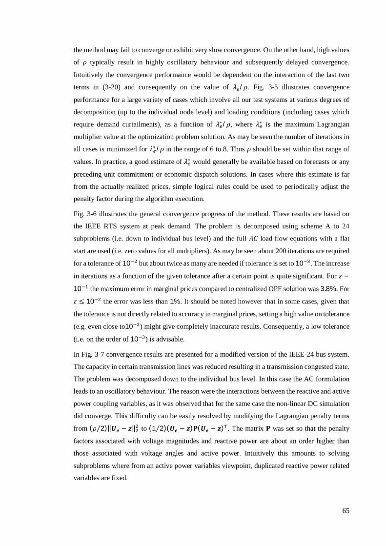
65
the method may fail to converge or exhibit very slow convergence. On the other hand, high values
of 휌 typically result in highly oscillatory behaviour and subsequently delayed convergence.
Intuitively the convergence performance would be dependent on the interaction of the last two
terms in (3-20) and consequently on the value of 휆 /휌. Fig. 3-5 illustrates convergence
performance for a large variety of cases which involve all our test systems at various degrees of
decomposition (up to the individual node level) and loading conditions (including cases which
require demand curtailments), as a function of 휆∗/휌, where 휆∗ is the maximum Lagrangian
multiplier value at the optimization problem solution. As may be seen the number of iterations in
all cases is minimized for 휆∗/휌 in the range of 6 to 8. Thus 휌 should be set within that range of
values. In practice, a good estimate of 휆∗ would generally be available based on forecasts or any
preceding unit commitment or economic dispatch solutions. In cases where this estimate is far
from the actually realized prices, simple logical rules could be used to periodically adjust the
penalty factor during the algorithm execution.
Fig. 3-6 illustrates the general convergence progress of the method. These results are based on
the IEEE RTS system at peak demand. The problem is decomposed using scheme A to 24
subproblems (i.e. down to individual bus level) and the full 퐴퐶 load flow equations with a flat
start are used (i.e. zero values for all multipliers). As may be seen about 200 iterations are required
for a tolerance of 10 but about twice as many are needed if tolerance is set to 10 . The increase
in iterations as a function of the given tolerance after a certain point is quite significant. For 휀 =
10 the maximum error in marginal prices compared to centralized OPF solution was 3.8%. For
휀 ≤ 10 the error was less than 1%. It should be noted however that in some cases, given that
the tolerance is not directly related to accuracy in marginal prices, setting a high value on tolerance
(e.g. even close to10 ) might give completely inaccurate results. Consequently, a low tolerance
(i.e. on the order of 10 ) is advisable.
In Fig. 3-7 convergence results are presented for a modified version of the IEEE-24 bus system.
The capacity in certain transmission lines was reduced resulting in a transmission congested state.
The problem was decomposed down to the individual bus level. In this case the AC formulation
leads to an oscillatory behaviour. The reason were the interactions between the reactive and active
power coupling variables, as it was observed that for the same case the non-linear DC simulation
did converge. This difficulty can be easily resolved by modifying the Lagrangian penalty terms
from (휌 2⁄ )‖푼풆 − 풛‖ to (1 2⁄ )(푼풆 − 풛)횸(푼풆 − 풛) . The matrix 횸 was set so that the penalty
factors associated with voltage magnitudes and reactive power are about an order higher than
those associated with voltage angles and active power. Intuitively this amounts to solving
subproblems where from an active power variables viewpoint, duplicated reactive power related
variables are fixed.

66
3.4.3 Effects of System Size
In this set of tests two non-convex cases are tested: a full AC and a non-linear DC type of
formulation derived by simply setting voltages to unity. The test systems include the IEEE-24,
57, 118, 300 test systems (data available on [161]) and a 707 buses system resembling the UK
network (data made available through personal communication with professor Janusz Bialek).
For the latter there are no reactive power data available. Each test system was decomposed to an
increasing number of subproblems. While this degree of decomposition might not seem to be of
practical interest, its theoretical investigation is, as a single bus could be thought of as an area
which could actually contain many more nodes and subsystems. Fig. 3-8 shows the results when
using the full AC equations, while the results with nonlinear DC equations are presented in Fig.
3-9. As may be expected, as the number of agents / subproblems increases, the number of
iterations to convergence also tends to increase. It is of note that each system scales differently,
Fig. 3-5: Effect of penalty factor on iterations to convergence for a tolerance 휀 ≤ 10 with fixed 휌.
Fig. 3-6: Effect of convergence tolerance value on iterations for a penalty factor 휌 = 10.
Fig. 3-7: Convergence in a congested case with uniform (left) and non-uniform (right) penalty factors.
0 5 10 15 20 25 300
500
1000
1500
e* /
itera
tions
0 200 400 600 800
0
20
40
60
iteration
mar
gina
l pric
e (m
.u./M
Wh)
<10-3 <10-4<10-2<10-1
0 2000 40000
20
40
60
80
100
iteration
mar
gina
l pric
e (m
.u./M
Wh)
0 2000 40000
20
40
60
80
100
iteration
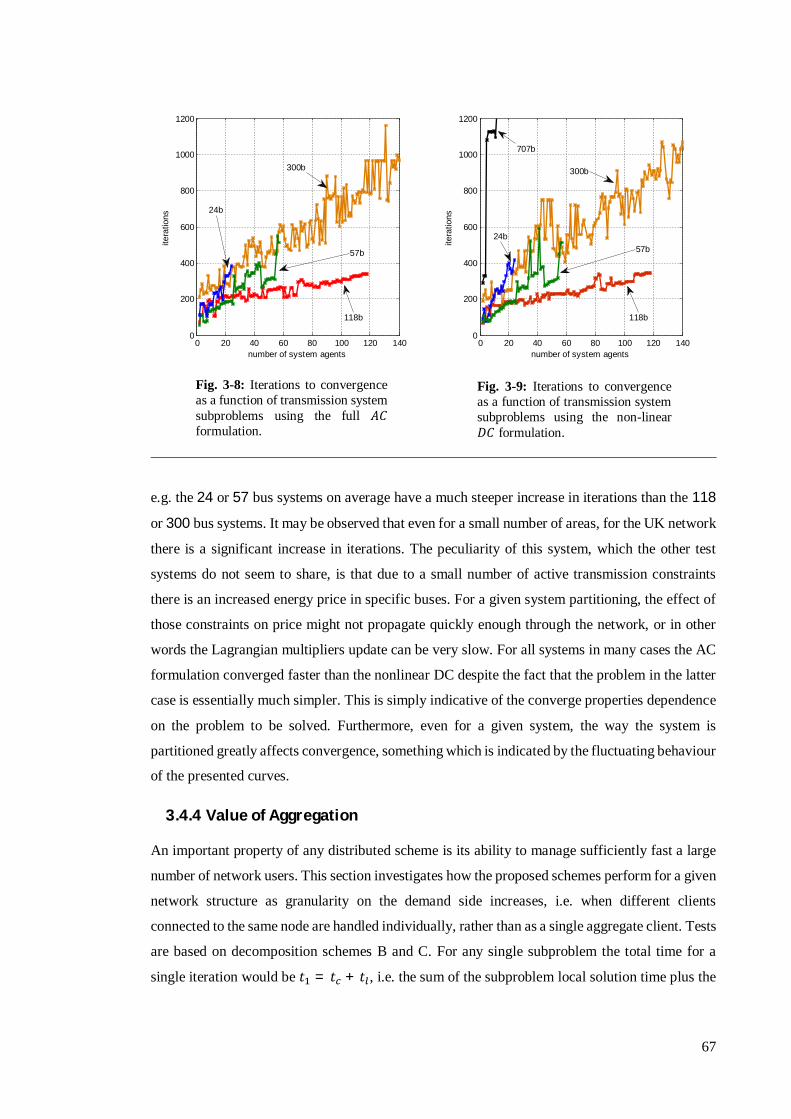
67
e.g. the 24 or 57 bus systems on average have a much steeper increase in iterations than the 118
or 300 bus systems. It may be observed that even for a small number of areas, for the UK network
there is a significant increase in iterations. The peculiarity of this system, which the other test
systems do not seem to share, is that due to a small number of active transmission constraints
there is an increased energy price in specific buses. For a given system partitioning, the effect of
those constraints on price might not propagate quickly enough through the network, or in other
words the Lagrangian multipliers update can be very slow. For all systems in many cases the AC
formulation converged faster than the nonlinear DC despite the fact that the problem in the latter
case is essentially much simpler. This is simply indicative of the converge properties dependence
on the problem to be solved. Furthermore, even for a given system, the way the system is
partitioned greatly affects convergence, something which is indicated by the fluctuating behaviour
of the presented curves.
3.4.4 Value of Aggregation
An important property of any distributed scheme is its ability to manage sufficiently fast a large
number of network users. This section investigates how the proposed schemes perform for a given
network structure as granularity on the demand side increases, i.e. when different clients
connected to the same node are handled individually, rather than as a single aggregate client. Tests
are based on decomposition schemes B and C. For any single subproblem the total time for a
single iteration would be 푡 = 푡 + 푡 , i.e. the sum of the subproblem local solution time plus the
Fig. 3-8: Iterations to convergence as a function of transmission system subproblems using the full 퐴퐶 formulation.
Fig. 3-9: Iterations to convergence as a function of transmission system subproblems using the non-linear 퐷퐶 formulation.
0 20 40 60 80 100 120 1400
200
400
600
800
1000
1200
number of system agents
itera
tions
24b
300b
118b
57b
0 20 40 60 80 100 120 1400
200
400
600
800
1000
1200
number of system agents
itera
tions
707b
300b
24b57b
118b

68
communications latency time (time required for sending the information to another agent). The
total execution time for scheme B and C may be given by the following relations:
푡 = ∑ max 푡 ( ), 푡 ( ) … , 푡 ( ), 푡 ( ), … ( 3–31)
푡 = ∑ max 푡 ( ), 푡 ( ) … , 푡 ( ∗), 푡 ( ∗), … ( 3–32)
푡 ( ∗) = ∑ max 푡 ( ), 푡 ( ), … + 푡 ( ) ( 3–33)
The operator Σ denotes summation over all iterations. Currently there is no fully fledged
communications standard for the smart grid, and as such it is difficult to predict latency values.
Therefore, in the examples that follow, we assume for all subproblems 푡 = 0.1푠. This may be
considered to represent the maximum latency time expected to be observed. In the following
paragraphs we investigate the comparative performance of the two decomposition schemes
assuming a single TSO agent. Our test results are illustrated in Fig. 3-10 and involve the
disaggregation of demand to an increasing number of MO problems by randomly breaking down
the initial demand blocks. Parameters for the decomposition algorithms were set based on the
guidelines of the previous sections.
Case 1 (IEEE RTS 24bus system – base data): In this case the TSO subproblem is small in size
and solved fast. The solution of DSO* subproblems takes typically longer. For a fixed penalty
factor value, iterations for scheme B increase roughly linearly. To a certain extent this may
be expected as due to the smaller demand block sizes, primal residuals tend to be smaller and
consequently so are the Lagrangian multiplier updates. On the other hand, the performance of
scheme C is roughly independent of the number of clients as the iterations remain constant.
This is due to two reasons: 1) independently of the degree of demand disaggregation iterations
at the TSO level remain constant; 2) the proximal decomposition algorithm is close in
principle to a price-based decomposition and thanks to its adaptive penalty update scheme is
not significantly affected by the number of subproblems. For small degrees of user
disaggregation scheme B performs better as it does not involve the additional round of
communications required for the solution of DSO* subproblems. For high degrees of
decomposition scheme C outperforms scheme B.
Case 2 (IEEE RTS 24bus system – contingency): In this case a few generators are assumed to
be on outage due to a fault. Demand curtailments are required and as such demand sets the
price. This implies strong interactions between MO subproblems during convergence which
could make the proximal algorithm convergence more difficult. While some increase may be
observed in terms of total time for scheme C, convergence time is much better than scheme
B. It should be noted that compared to the previous case convergence time is also increased.
This is typical behaviour of ADMM when it has to converge to a particularly high price (in
this case the VOLL associated with users). The reason for this, is that the difference in power
schedules between the TSO and MOs determined by the solution of (3-21), would typically

69
be limited by the power constraints involved in the associated subproblems. This power
difference however has to be used in the Lagrange multiplier update in (3-23). Depending on
the penalty factor value, a significant number of iterations might be required to converge, if
the optimum Lagrange multiplier value is far from the initial point.
Case 3 (IEEE 300bus system – base data): This case differs from the first in that the TSO
problem is much larger and its solution takes longer. In this case DSO* subproblems are faster
to solve, thus the number of TSO-level iterations determines the overall convergence time.
As may be seen scheme C practically outperforms scheme B in every case.
It should be noted that in all the above test cases the linear increase in iterations for scheme B
actually represents a worst case performance, as convergence could be potentially improved
through a suitable modification of the ADMM penalty factors. However, this could be challenging
to do for different operating cases in a system without affecting the TSO-level iterations. For large
systems this is particularly important as a larger number of iterations at that level directly implies
an increased convergence time. In addition, it should be noted that a more complex and accurate
latency model would probably reinforce our conclusions as the communications burden for
scheme B is generally higher than that of scheme C. This would also be the case if the results
were to be produced using different solvers or equipment (in this case an Intel Core i5-2500
3.3Ghz, with 4GB of RAM was used).
It is well-known that aggregators are considered to be a fundamental part of the future smart grid
[96]. The way these are organized and the algorithms they utilize will have a significant impact
on the convergence speed of any decentralized power system operation scheme. Given that the
point of delivery of energy in a power system does matter, a collection of microgrids combined
with distribution network aggregators could be the natural basis for decentralized power systems
operations in the future. As it is, our results indicate that this is indeed an efficient decomposition
structure from a distributed optimization perspective, where increased granularity in demand does
not necessarily imply slower convergence.
Fig. 3-10: Time to convergence for three different test cases for decomposition schemes B and C. As may be seen scheme C consistently outperforms scheme B as the degree of disaggregation increases.
0 500 1000 15000
5
10
15
conv
erge
nce
time
(min
)
0 500 1000 15000
5
10
15
number of MO agents0 2000 4000 6000 8000
0
5
10
15scheme Bscheme C
300b-normal24b-normal 24b-contingency

70
3.4.5 Convergence Considerations
ADMM has been proven to converge only for convex problems, whereas the OPF problem is a
non-linear and non-convex one. As reference [125] points out, convergence for non-convex cases
cannot be guaranteed. The results presented in Fig. 3-6 are indicative of this fact. On the other
hand, for a suitable selection of penalty factors, the method always converged. In terms of
optimality, again as [125] points out, the method should be considered as a local optimization
method, and as such its performance is dependent on the initial conditions. This however does not
imply any worse performance than centralized methods [162]. This was also verified through our
simulation results, where the solution of both centralized (interior point method based) and
distributed (ADMM-based) approaches was the essentially the same. Overall, while a
mathematical convergence proof cannot be provided for the general non-convex case, our
extensive simulation results indicate that ADMM can work reliably for the OPF problem,
independently of its formulation. Of course, if the recent efforts in convexifying the OPF problem
(as discussed in the previous chapter) find general application then any such convergence issues
would be obsolete.
Another question of interest is convergence performance in degenerate cases. As indicated in
[163] there are two common types of degeneracy in the OPF problem, related to controls and
constraints. Control degenerate cases were included in our test set (e.g. load curtailment cases
where multiple demand blocks at a single bus were marginal at the same time). This type of
degeneracy is resolved through the quadratic terms included in the subproblems and convergence
can be ensured. On the other hand, constraint degenerate cases were not involved in our tests.
Such cases are difficult to identify but could appear on more complex formulations of the problem
with more complex market rules. Relevant investigation could be a direction for future research.
3.5 Conclusions & Further Questions
The results of this chapter may again be summarized in the updated energy management
schematic shown on Fig. 3-11. Compared to Fig. 2-5 the centralized economic dispatch approach
has been replaced by our two-level hierarchical decentralized approach to OPF. While only
limited degrees of network decomposition appear to be feasible, through this structure a
significant degree of users disaggregation is possible. This in turn would allow considering in
detail the latter’s individual constraints and objectives.
While the presented results regarding network decomposition apply in both transmission and
distribution networks (or a combination of both) It should be noted that in this chapter we have
not yet explicitly discussed where and how distribution network constraints would be represented

71
in their full detail, and we have not yet covered the time-coupling aspects of demand. These are
questions that will be answered in the following chapter.
Fig. 3-11: The updated schematic from chapter 2. Microgrids are a new structural element in the energy management problem.

73
4 Extended Economic Dispatch
This chapter extends the optimal power flow formulation to account for the distribution network constraints and incorporate the time-linkages of flexible demand, while associating it with the economic dispatch problem. This gives a quite specific perspective on how distributed optimization methods fit in power systems operation.
4.1 Extended Economic Dispatch
Economic dispatch is the basic mechanism used to determine close to real-time the operating set-
points of all controllable devices connected in the power system in an economically efficient way.
In its traditional form, the OPF formulation presented in chapter 2 forms its basis. However, that
is not adequate when deferrable demand is taken into account. The value of energy purchased by
an EV or storage unit now, depends on the price of energy in the future, which is typically
determined by the large generating units located at the transmission level. As [164] has shown,
insufficient coordination between demand shifting decisions and generation scheduling can result
in increased energy price volatility. In addition, the increased flexible demand (mainly in the form
of EVs), will put considerable strain on existing power distribution infrastructure. If that demand
is properly managed while taking into account distribution grid limitations, then investments
could be deferred giving significant financial benefits. As a consequence, the balancing market
(with the associated economic dispatch problem) should not only determine the price and optimal
amount of energy trades for the current time-step (as it currently does) but also provide a good
indication of the demand shifting impact on the value of energy in the near future. Furthermore,
it would have to incorporate the constraints and peculiarities of distribution networks.
The reasoning of the aforementioned paragraph leads to two basic considerations: 1) in order to
account for the time-linkages of flexible demand (and generator ramp rates) optimization has to
be carried over a time-period comparable to the time an individual flexible device (e.g. an EV) is
available to be controlled (e.g. 8-14 hours); 2) over such a period of time there will be uncertainty
related to a variety of factors such as: the output of renewable generation; power required by
inflexible demand; energy requirements as well as arrival and departure times of EVs. Thus, a
comprehensive way to describe our problem would be through a multi-period stochastic
programming formulation, where uncertainty is modelled through a set of scenarios describing
possible system states:
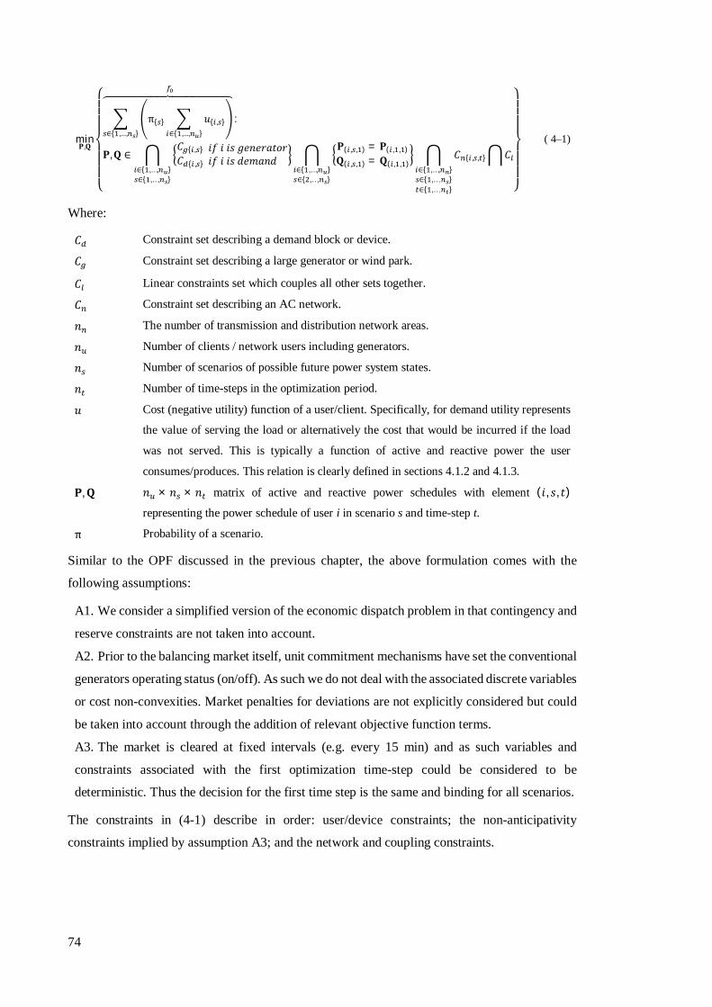
74
min퐏,퐐
⎩⎪⎪⎪⎨
⎪⎪⎪⎧
π{ } 푢{ , }∈{ ,..., }∈{ ,..., }
:
퐏,퐐 ∈퐶 { , }퐶 { , }
푖푓 푖 푖푠 푔푒푛푒푟푎푡표푟푖푓 푖 푖푠 푑푒푚푎푛푑
∈{ ,…, }∈{ ,…, }
퐏( , , ) = 퐏( , , )퐐( , , ) = 퐐( , , )
∈{ ,…, }∈{ ,…, }
퐶 { , , }∈{ ,…, }∈{ ,…, }∈{ ,…, }
퐶
⎭⎪⎪⎪⎬
⎪⎪⎪⎫
( 4–1)
Where:
퐶 Constraint set describing a demand block or device.
퐶 Constraint set describing a large generator or wind park.
퐶 Linear constraints set which couples all other sets together.
퐶 Constraint set describing an AC network.
푛 The number of transmission and distribution network areas.
푛 Number of clients / network users including generators.
푛 Number of scenarios of possible future power system states.
푛 Number of time-steps in the optimization period.
푢 Cost (negative utility) function of a user/client. Specifically, for demand utility represents
the value of serving the load or alternatively the cost that would be incurred if the load
was not served. This is typically a function of active and reactive power the user
consumes/produces. This relation is clearly defined in sections 4.1.2 and 4.1.3.
퐏,퐐 푛 × 푛 × 푛 matrix of active and reactive power schedules with element (푖, 푠, 푡)
representing the power schedule of user i in scenario s and time-step t.
π Probability of a scenario.
Similar to the OPF discussed in the previous chapter, the above formulation comes with the
following assumptions:
A1. We consider a simplified version of the economic dispatch problem in that contingency and
reserve constraints are not taken into account.
A2. Prior to the balancing market itself, unit commitment mechanisms have set the conventional
generators operating status (on/off). As such we do not deal with the associated discrete variables
or cost non-convexities. Market penalties for deviations are not explicitly considered but could
be taken into account through the addition of relevant objective function terms.
A3. The market is cleared at fixed intervals (e.g. every 15 min) and as such variables and
constraints associated with the first optimization time-step could be considered to be
deterministic. Thus the decision for the first time step is the same and binding for all scenarios.
The constraints in (4-1) describe in order: user/device constraints; the non-anticipativity
constraints implied by assumption A3; and the network and coupling constraints.

75
4.1.1 Network Constraints
We assume that the network is separated to areas. A single area may represent part of the
transmission and/or distribution network. The most straightforward way to describe an arbitrary
ac network is through the standard set of ac constraints (in complex numbers notation):
퐶 { , , } =
⎩⎨
⎧퐒 { , , } = 푑푖푎푔 퐕{ , , } 퐘{ }퐕{ , , }∗
퐕{ } ≤ 퐕{ , , } ≤ 퐕{ }
퐘 { }퐕{ , , } ≤ 퐈 { } ⎭⎬
⎫ ( 4–2)
Where:
푛 The number of buses/nodes in the network.
퐒 Bus apparent power injection 푛 × 1 vector.
퐈 Line current limit vector.
퐕 Bus voltages 푛 × 1 vector. 퐕 and 퐕 denote the upper and lower bounds on voltage
magnitude respectively.
퐘,퐘 Bus admittance and line flow admittance matrix respectively.
The equations describe in order: bus power balance; voltage magnitude constraints; line capacity
constraints.
4.1.2 Generation Constraints
For a generating unit the relevant constraints are described by the following set of equations:
퐶 { , } =
⎩⎪⎪⎨
⎪⎪⎧ 푢{ , } = 푐 { }퐏( , , ) + 푐 { }퐏( , , )
∈[ , ]
푃{ , , } ≤ 퐏( , , ) ≤ 푃{ , , } ∀ 푡 ∈ {1, … , 푛 }
푄{ } ≤ 퐐( , , ) ≤ 푄{ } ∀ 푡 ∈ {1, … ,푛 }
푃 { , } ≤ 퐏( , , ) −퐏( , , ) ≤ 푃 { , } ∀ 푡 ∈ {2, … , 푛 }⎭⎪⎪⎬
⎪⎪⎫
( 4–3)
Where:
푐 , 푐 Active power variable cost coefficients. In power systems literature these are typically
assumed to be quadratic (further information may be found in [165]). However, this is not
restrictive in our formulation and any other function may be used instead. Additional
utility terms could be added relating to reactive power provision.
푃 Ramp rate limits.
For a conventional generator power limits are the same for any value of the index s. For a
renewable generator the lower bound is zero, the upper bound varies following a given forecast
error distribution (e.g. [166]), while the ramp rate-constraint is redundant.
4.1.3 Demand Constraints
For user-level demand / devices the constraints are:

76
퐶 { , } =
⎩⎪⎪⎨
⎪⎪⎧푢{ , } = max 푐 { } 퐸{ , , } −퐸 { , , } , 0
∈[ , ]
푃{ , , } ≤ 퐏( , , ) ≤ 푃{ , , } ∀ 푡 ∈ {1, … ,푛 }
퐸{ , , } = 퐸{ , , } + 푐 퐏( , , ) ∀ 푡 ∈ {1, … ,푛 }퐸{ , } ≤ 퐸{ , , } ≤ 퐸{ , } ∀ 푡 ∈ {1, … ,푛 }
퐐( , , ) = 퐏( , , ) 푡푎푛휙 ∀ 푡 ∈ {1, … , 푛 } ⎭⎪⎪⎬
⎪⎪⎫
( 4–4)
Where:
푐 The cost of shedding demand (value of lost load).
푐 Factor accounting for energy conversion losses.
휙 Angle between active and reactive power.
퐸 Energy stored at the end of a time step. We assume that 퐸{ , , }=0 and that the energy
bounds have been appropriately shifted.
퐸 Energy target at a given time step. Note that by definition demand is negative, thus the
utility function penalizes cases where energy consumed is less than the desired.
In this work we consider the following types of demand / devices which are adequately modelled
by the above equations:
Inflexible demand: The upper power bound would be 0, and the lower would vary in different
scenarios following a certain forecast error. Energy bounds are redundant, while 퐸 { , , } =
∑ 푃{ , , }∈[ , ] and 0 for all other time steps.
Small scale renewables: These are simply assumed to be negative demand (i.e. 0 lower bound
on power and 푐 = 0)
Electric vehicles: For an EV 퐸 represents the energy requirements for travelling purposes.
Power bounds are set to 0 if the vehicle is not connected. Typical probability distributions for
vehicle connection / disconnection times and energy requirements may be found e.g. in [167].
We do not model self-discharge energy losses for battery systems as these typically amount to
less than 5% during the first 24h [168], and are unlikely to affect a system-wide optimization
results. Based on [169, 170] we assume that the majority of EVs operate in a unidirectional
manner.
The reasoning behind focusing on these particular devices is that their combined use would likely
be the main cause of issues with respect to distribution network operation. However, there is a
number of other types of demand that have their own role to play in energy management such as:
storage (battery based storage is actually covered by the above), household wet appliances,
heating systems, industrial processes, etc. Modelling the flexibility of each individual type of
device/demand is a considerable task that goes beyond the purposes of this work. However our
formulation and solution approach are generic and it is easy to add additional constraint sets or
modify existing ones.
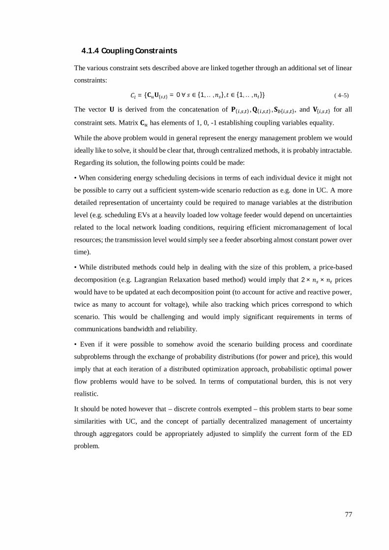
77
4.1.4 Coupling Constraints
The various constraint sets described above are linked together through an additional set of linear
constraints:
퐶 = {퐂 퐔{ , } = 0 ∀ 푠 ∈ {1, … ,푛 }, 푡 ∈ {1, … ,푛 }} ( 4–5)
The vector 퐔 is derived from the concatenation of 퐏( , , ),퐐( , , ), 퐒 { , , }, and 퐕{ , , } for all
constraint sets. Matrix 퐂 has elements of 1, 0, -1 establishing coupling variables equality.
While the above problem would in general represent the energy management problem we would
ideally like to solve, it should be clear that, through centralized methods, it is probably intractable.
Regarding its solution, the following points could be made:
• When considering energy scheduling decisions in terms of each individual device it might not
be possible to carry out a sufficient system-wide scenario reduction as e.g. done in UC. A more
detailed representation of uncertainty could be required to manage variables at the distribution
level (e.g. scheduling EVs at a heavily loaded low voltage feeder would depend on uncertainties
related to the local network loading conditions, requiring efficient micromanagement of local
resources; the transmission level would simply see a feeder absorbing almost constant power over
time).
• While distributed methods could help in dealing with the size of this problem, a price-based
decomposition (e.g. Lagrangian Relaxation based method) would imply that 2 × 푛 × 푛 prices
would have to be updated at each decomposition point (to account for active and reactive power,
twice as many to account for voltage), while also tracking which prices correspond to which
scenario. This would be challenging and would imply significant requirements in terms of
communications bandwidth and reliability.
• Even if it were possible to somehow avoid the scenario building process and coordinate
subproblems through the exchange of probability distributions (for power and price), this would
imply that at each iteration of a distributed optimization approach, probabilistic optimal power
flow problems would have to be solved. In terms of computational burden, this is not very
realistic.
It should be noted however that – discrete controls exempted – this problem starts to bear some
similarities with UC, and the concept of partially decentralized management of uncertainty
through aggregators could be appropriately adjusted to simplify the current form of the ED
problem.
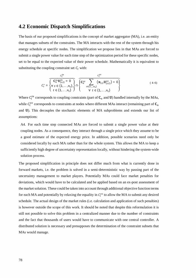
78
4.2 Economic Dispatch Simplifications
The basis of our proposed simplifications is the concept of market aggregator (MA), i.e. an entity
that manages subsets of the constraints. The MA interacts with the rest of the system through his
energy schedule at specific nodes. The simplification we propose lies in that MAs are forced to
submit a single power value for each time step of the optimization period for these specific nodes,
set to be equal to the expected value of their power schedule. Mathematically it is equivalent to
substituting the coupling constraint set 퐶 with:
퐶∗ =퐂 퐔{ , } = 0
∀ 푠 ∈ {1, … ,푛 },푡 ∈ {1, … , 푛 }
∩퐂 훑( )퐔{ , }
∈{ ,..., }
= 0
∀ 푡 ∈ {1, … , 푛 }
( 4–6)
Where 퐶 corresponds to coupling constraints (part of 퐂 and 퐔) handled internally by the MAs,
while 퐶 corresponds to constraints at nodes where different MAs interact (remaining part of 퐂
and 퐔). This decouples the stochastic elements of MA subproblems and extends our list of
assumptions:
A4. For each time step connected MAs are forced to submit a single power value at their
coupling nodes. As a consequence, they interact through a single price which they assume to be
a good estimate of the expected energy price. In addition, possible scenarios need only be
considered locally by each MA rather than for the whole system. This allows the MA to keep a
sufficiently high degree of uncertainty representation locally, without hindering the system-wide
solution process.
The proposed simplification in principle does not differ much from what is currently done in
forward markets, i.e. the problem is solved in a semi-deterministic way by passing part of the
uncertainty management to market players. Potentially MAs could face market penalties for
deviations, which would have to be calculated and be applied based on an ex-post assessment of
the market solution. These could be taken into account through additional objective function terms
for each MA and potentially by relaxing the equality in 퐶 to allow the MA to submit any desired
schedule. The actual design of the market rules (i.e. calculation and application of such penalties)
is however outside the scope of this work. It should be noted that despite this reformulation it is
still not possible to solve this problem in a centralized manner due to the number of constraints
and the fact that thousands of users would have to communicate with one central controller. A
distributed solution is necessary and presupposes the determination of the constraint subsets that
MAs would manage.

79
4.2.1 Market Aggregator Structure
The overall multi-period problem structure may be visualized on the table-like structure of Fig.
4-1. As may be observed the problem has a hierarchical structure which is indicative of how it
should be decomposed and of the interrelations between the generated subproblems. First a
number of MAs would be managing parts of the transmission system. As such we have the
transmission system operator (푀퐴 ) type of subproblems which manage subsets of the
transmission constraints. Linked with them are the problems of distribution system operators
(푀퐴 ) managing parts of the distribution network at a specific bus, and the problems of
independent large generators (푀퐴 ). At an even lower level one could find a small number of
medium voltage nodes and/or all users at a low voltage feeder managed by a microgrid operator
(푀퐴 ). The initial optimization problem may be decomposed into these general types of
subproblems. At this point we further extend the assumptions regarding our solution approach:
A5. Each MA is equipped with a digital device which solves a generic subproblem formulation
(as described in the next section) and handles the necessary communications with the rest of the
system. Constraint parameters values and forecasts are provided by the user / aggregator but
changes are not possible during an optimization run.
Fig. 4-1: Left: Schematic representation of involved constraint sets. Each block represents a constraint set. The columns and rows correspond to time-steps and constraint set type respectively. There is a third dimension to this table as multiple copies of the same constraint type may exist (indicated by blocks piled on top of each other). Each arrow-line indicates coupling between sets (part of 퐶 ). Note that blocks with time-linkage constraints, e.g. flexible demand (퐶 ), cover multiple columns. For the illustrated example there exist three copies of 퐶 for each time-step at the transmission level. The constraint set of area 1 is linked with the distribution constraints of buses 2 and 4, the generators at bus 2 and the other two transmission area constraint sets. The distribution network constraint set of bus 4 is in turn linked with various low voltage network constraint sets and the individual users. Right: Schematic representation of the underlying decomposition structure. Each block represents a market aggregator and arrow-lines indicate coupling and required bi-directional communications links.

80
A6. The size of an MO is such that the uncertainty regarding its expected power schedule can
be reasonably small. From a market perspective this size could be indirectly determined through
imposed penalties for deviations. Following [171] we assume that marginal pricing is also
applied to 푀푂s.
4.2.2 Decentralized Solution
With respect to the decomposition structure at the transmission level the following observations
may be made:
• As the analysis of distributed solutions for the OPF problem indicates, for large degrees of
decomposition especially in certain congested or contingent cases convergence can be slow [172].
In addition, contingency constraints typically involved in ED are not necessarily easy to
decompose. Thus it can be expected that at this level decomposition would be limited to a rather
small number of areas implying that TSO subproblems would remain computationally intensive.
• Following the above, it is of interest to limit as much as possible iterations at this level (i.e.
number of TSO problems that have to be solved). However, these are bound to increase with
increasing disaggregation (i.e. larger number of MOs) [172]. At the same time however it is also
of interest to disaggregate demand and represent it in as much detail as reasonably possible, given
that ED is the last attempt to coordinate resources system-wide in an economically optimal way.
Any dispatch / control mechanisms that follow would have to act locally and as a consequence
cannot possibly be optimal in that same sense.
As a consequence, we will retain here the two level decomposition structure introduced in the
previous chapter. This would give four types of subproblems. For each 푀퐴 we have the
following subproblem:
min퐱풂
훌 : 퐱 :
+ 휌‖퐱 : − 퐳 ‖
:퐱 ∈ 퐶 { , , } ∩ 퐶 :
∗ ∀ 푠 ∈ {1, … ,푛 }, 푡 ∈ {1, … ,푛 } ( 4–7)
The index ‘a’ indicates subsets of variables and sets managed by the aggregator. For each 푀퐴
we have:
min퐱풂
푓 : (퐱 )
+ 훌 : 퐱 :
+ 휌‖퐱 : − 퐳 ‖
:퐱 ∈ 퐶 { , } ∩ 퐶 :
∗ ∀ 푠 ∈ {1, … ,푛 } ( 4–8)
For each 푀퐴 we have:
min풙
⎩⎪⎪⎨
⎪⎪⎧
훌 : 퐱 :
+ 휌‖퐱 : − 퐳 ‖
+
+ 훌 : 퐱 :
+ 휌 ‖퐱 : − 퐳 ‖
:퐱 ∈ 퐶 { , , } ∩ 퐶 :
∗ ∀ 푠 ∈ {1, … ,푛 }, 푡 ∈ {1, … ,푛 }⎭⎪⎪⎬
⎪⎪⎫
( 4–9)
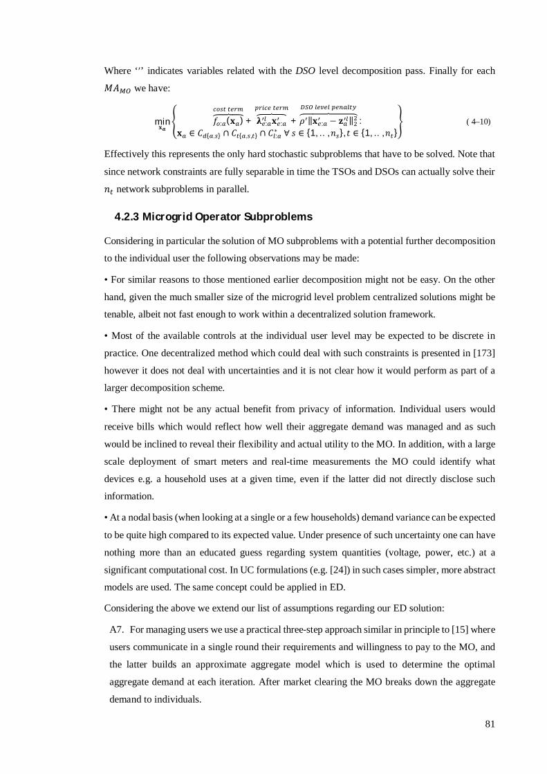
81
Where ‘′’ indicates variables related with the DSO level decomposition pass. Finally for each
푀퐴 we have:
min퐱풂
푓 : (퐱 )
+ 훌 : 퐱 :
+ 휌 ‖퐱 : − 퐳 ‖
:퐱 ∈ 퐶 { , } ∩ 퐶 { , , } ∩ 퐶 :
∗ ∀ 푠 ∈ {1, … ,푛 }, 푡 ∈ {1, … ,푛 } ( 4–10)
Effectively this represents the only hard stochastic subproblems that have to be solved. Note that
since network constraints are fully separable in time the TSOs and DSOs can actually solve their
푛 network subproblems in parallel.
4.2.3 Microgrid Operator Subproblems
Considering in particular the solution of MO subproblems with a potential further decomposition
to the individual user the following observations may be made:
• For similar reasons to those mentioned earlier decomposition might not be easy. On the other
hand, given the much smaller size of the microgrid level problem centralized solutions might be
tenable, albeit not fast enough to work within a decentralized solution framework.
• Most of the available controls at the individual user level may be expected to be discrete in
practice. One decentralized method which could deal with such constraints is presented in [173]
however it does not deal with uncertainties and it is not clear how it would perform as part of a
larger decomposition scheme.
• There might not be any actual benefit from privacy of information. Individual users would
receive bills which would reflect how well their aggregate demand was managed and as such
would be inclined to reveal their flexibility and actual utility to the MO. In addition, with a large
scale deployment of smart meters and real-time measurements the MO could identify what
devices e.g. a household uses at a given time, even if the latter did not directly disclose such
information.
• At a nodal basis (when looking at a single or a few households) demand variance can be expected
to be quite high compared to its expected value. Under presence of such uncertainty one can have
nothing more than an educated guess regarding system quantities (voltage, power, etc.) at a
significant computational cost. In UC formulations (e.g. [24]) in such cases simpler, more abstract
models are used. The same concept could be applied in ED.
Considering the above we extend our list of assumptions regarding our ED solution:
A7. For managing users we use a practical three-step approach similar in principle to [15] where
users communicate in a single round their requirements and willingness to pay to the MO, and
the latter builds an approximate aggregate model which is used to determine the optimal
aggregate demand at each iteration. After market clearing the MO breaks down the aggregate
demand to individuals.
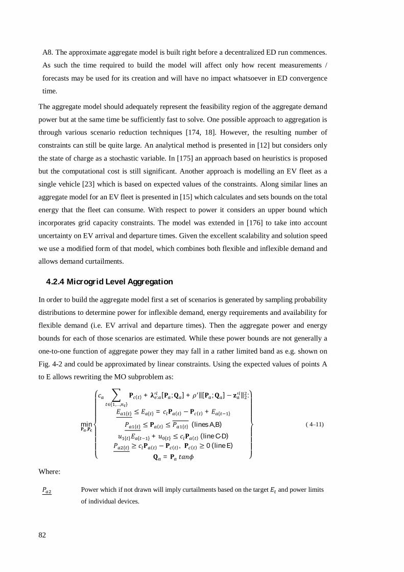
82
A8. The approximate aggregate model is built right before a decentralized ED run commences.
As such the time required to build the model will affect only how recent measurements /
forecasts may be used for its creation and will have no impact whatsoever in ED convergence
time.
The aggregate model should adequately represent the feasibility region of the aggregate demand
power but at the same time be sufficiently fast to solve. One possible approach to aggregation is
through various scenario reduction techniques [174, 18]. However, the resulting number of
constraints can still be quite large. An analytical method is presented in [12] but considers only
the state of charge as a stochastic variable. In [175] an approach based on heuristics is proposed
but the computational cost is still significant. Another approach is modelling an EV fleet as a
single vehicle [23] which is based on expected values of the constraints. Along similar lines an
aggregate model for an EV fleet is presented in [15] which calculates and sets bounds on the total
energy that the fleet can consume. With respect to power it considers an upper bound which
incorporates grid capacity constraints. The model was extended in [176] to take into account
uncertainty on EV arrival and departure times. Given the excellent scalability and solution speed
we use a modified form of that model, which combines both flexible and inflexible demand and
allows demand curtailments.
4.2.4 Microgrid Level Aggregation
In order to build the aggregate model first a set of scenarios is generated by sampling probability
distributions to determine power for inflexible demand, energy requirements and availability for
flexible demand (i.e. EV arrival and departure times). Then the aggregate power and energy
bounds for each of those scenarios are estimated. While these power bounds are not generally a
one-to-one function of aggregate power they may fall in a rather limited band as e.g. shown on
Fig. 4-2 and could be approximated by linear constraints. Using the expected values of points A
to E allows rewriting the MO subproblem as:
min퐏 ,퐏퐜
⎩⎪⎪⎪⎨
⎪⎪⎪⎧푐 퐏 ( )
∈{ ,…, }
+ 훌 : [퐏 ;퐐 ] + 휌 ‖[퐏 ;퐐 ]− 퐳 ‖ :
퐸 { } ≤ 퐸 { } = 푐 퐏 ( ) −퐏 ( ) + 퐸 { }
푃 { } ≤ 퐏 ( ) ≤ 푃 { } (lines A,B)
푢 { }퐸 { } + 푢 { } ≤ 푐 퐏 ( ) (line C-D)푃 { } ≥ 푐 퐏 ( ) − 퐏 ( ), 퐏 ( ) ≥ 0 (line E)
퐐 = 퐏 푡푎푛휙 ⎭⎪⎪⎪⎬
⎪⎪⎪⎫
( 4–11)
Where:
푃 Power which if not drawn will imply curtailments based on the target 퐸 and power limits
of individual devices.
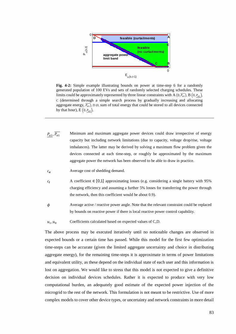
83
푃 , 푃 Minimum and maximum aggregate power devices could draw irrespective of energy
capacity but including network limitations (due to capacity, voltage drop/rise, voltage
imbalances). The latter may be derived by solving a maximum flow problem given the
devices connected at each time-step, or roughly be approximated by the maximum
aggregate power the network has been observed to be able to draw in practice.
푐풂 Average cost of shedding demand.
푐풍 A coefficient ∈ [0,1] approximating losses (e.g. considering a single battery with 95%
charging efficiency and assuming a further 5% losses for transferring the power through
the network, then this coefficient would be about 0.9).
휙 Average active / reactive power angle. Note that the relevant constraint could be replaced
by bounds on reactive power if there is local reactive power control capability.
푢 ,푢 Coefficients calculated based on expected values of C,D.
The above process may be executed iteratively until no noticeable changes are observed in
expected bounds or a certain time has passed. While this model for the first few optimization
time-steps can be accurate (given the limited aggregate uncertainty and choice in distributing
aggregate energy), for the remaining time-steps it is approximate in terms of power limitations
and equivalent utility, as these depend on the individual state of each user and this information is
lost on aggregation. We would like to stress that this model is not expected to give a definitive
decision on individual devices schedules. Rather it is expected to produce with very low
computational burden, an adequately good estimate of the expected power injection of the
microgrid to the rest of the network. This formulation is not meant to be restrictive. Use of more
complex models to cover other device types, or uncertainty and network constraints in more detail
Fig. 4-2: Simple example illustrating bounds on power at time-step 6 for a randomly generated population of 100 EVs and sets of randomly selected charging schedules. These limits could be approximately represented by three linear constraints with A 0, 푃 , B 0, 푃 ,
C (determined through a simple search process by gradually increasing and allocating aggregate energy, 푃 , D (0, sum of total energy that could be stored to all devices connected by that hour), E 0,푃 .
0
0
E{s,t-1}
P
{s,t} feasible
(no curtailments)
feasible (curtailments)
BC
E
D A
aggregate power limit band
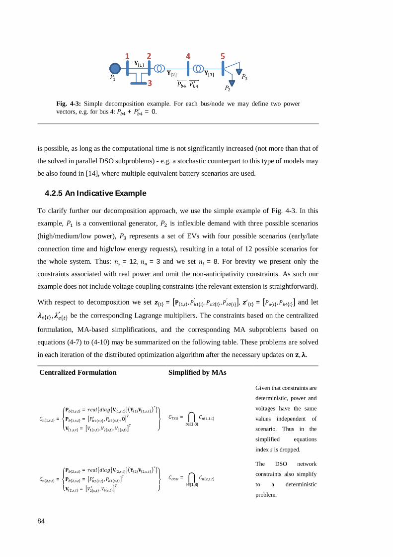
84
is possible, as long as the computational time is not significantly increased (not more than that of
the solved in parallel DSO subproblems) - e.g. a stochastic counterpart to this type of models may
be also found in [14], where multiple equivalent battery scenarios are used.
4.2.5 An Indicative Example
To clarify further our decomposition approach, we use the simple example of Fig. 4-3. In this
example, 푃 is a conventional generator, 푃 is inflexible demand with three possible scenarios
(high/medium/low power), 푃 represents a set of EVs with four possible scenarios (early/late
connection time and high/low energy requests), resulting in a total of 12 possible scenarios for
the whole system. Thus: 푛 = 12, 푛 = 3 and we set 푛 = 8. For brevity we present only the
constraints associated with real power and omit the non-anticipativity constraints. As such our
example does not include voltage coupling constraints (the relevant extension is straightforward).
With respect to decomposition we set 풛{ } = 퐏(1,푡),푃푏1{푡}′ ,푃푏2{푡},푃푏2{푡}
′ , 풛 { } = 푃푎{푡},푃푏4{푡} and let
흀 { },흀 { } be the corresponding Lagrange multipliers. The constraints based on the centralized
formulation, MA-based simplifications, and the corresponding MA subproblems based on
equations (4-7) to (4-10) may be summarized on the following table. These problems are solved
in each iteration of the distributed optimization algorithm after the necessary updates on 퐳,훌.
Centralized Formulation Simplified by MAs
퐶 { , , } =
⎩⎨
⎧퐏 { , , } = 푟푒푎푙 푑푖푎푔 퐕{ , , } 퐘{ }퐕{ , , }∗
퐏 { , , } = 푃 { , },푃 { , }, 0
퐕{ , , } = 푉 { , },푉 { , },푉 { , } ⎭⎬
⎫ 퐶 = 퐶 { , , }
푡∈[1,8]
Given that constraints are
deterministic, power and
voltages have the same
values independent of
scenario. Thus in the
simplified equations
index s is dropped.
퐶 { , , } =
⎩⎨
⎧퐏 { , , } = 푟푒푎푙 푑푖푎푔 퐕{ , , } 퐘{ }퐕{ , , }∗
퐏 { , , } = 푃 { , },푃 { , }
퐕{ , , } = 푉 { , },푉 { , } ⎭⎬
⎫ 퐶 = 퐶 { , , }
푡∈[1,8]
The DSO network
constraints also simplify
to a deterministic
problem.
Fig. 4-3: Simple decomposition example. For each bus/node we may define two power vectors, e.g. for bus 4: 푃 + 푃 = 0.

85
퐶 { , } =
⎩⎪⎨
⎪⎧푢{ , } = 푐 { }퐏( , , ) + 푐 { }퐏( , , )
∈[ , ]
푃{ } ≤ 퐏( , , ) ≤ 푃{ }
푃 { } ≤ 퐏( , , ) − 퐏( , , ) ≤ 푃 { } ⎭⎪⎬
⎪⎫
퐶 = 퐶 { , }
These are the constraints
of the generator. They too
become deterministic.
퐶 { , , } =
⎩⎨
⎧퐏 { , , } = 푟푒푎푙 푑푖푎푔 퐕{ , , } 퐘{ }퐕{ , , }∗
퐏 { , , } = 퐏 { , },퐏 { , }
퐕{ , , } = 퐕 { , },퐕 { , } ⎭⎬
⎫
퐶 { , } =푢{ , } = 푐 { } 퐏( , , )
∈[ , ]푃{ , , } ≤ 퐏( , , ) ≤ 0
퐶 { , } =푢{ , } = max 푐 { } 퐸{ , , } − 퐸 { , } , 0푃( , , ) ≤ 퐏( , , ) ≤ 0 퐸{ , } ≤ 퐸{ , , } = 퐸{ , , } + 푐 퐏( , , )
퐶 =
⎩⎪⎪⎪⎪⎨
⎪⎪⎪⎪⎧푃 { } = 훑( )
∈[1,12]
푃 { , }
퐶 { , , }푡∈[1,8]푠∈[1,12]
퐶 { , }푠∈[1,12]
퐶 { , }푠∈[1,12] ⎭
⎪⎪⎪⎪⎬
⎪⎪⎪⎪⎫
The constraints of the low
voltage network and the
two demand devices
combine into the
constraints of the MO.
This is still a stochastic
problem and the MO
interacts with the rest of
the network through 푃 .
Coupled with 퐶 these
would correspond to the
푀퐴∗ type of problem.
퐶 =
⎩⎪⎨
⎪⎧
⎣⎢⎢⎢⎡퐏( , , ) − 푆 { , }퐏( , , ) + 퐏( , , ) − 푃 { , }
푃 { , } + 푃 { , }
푃 { , } + 푃 { , } ⎦⎥⎥⎥⎤
= ퟎ
⎭⎪⎬
⎪⎫
퐶 =
⎩⎪⎨
⎪⎧
⎣⎢⎢⎢⎡퐏( , ) − 푃 { }푃 { } − 푃 { }
푃 { } + 푃 { }
푃 { } + 푃 { }⎦⎥⎥⎥⎤
= 0
⎭⎪⎬
⎪⎫
퐶 = 퐏( , , ) + 퐏( , , ) − 푃 { , } = 0
The coupling constraints
may be written as two
sets: 퐶 which is used in
the decomposition and
퐶 which is handled
internally by the MO.
Decomposition Subproblems
min퐱풂{ }≡ { }
{ }
훌 { }( ),훌 { }( ) 퐱 { } +
휌 퐱 { } − 퐳{ }( ),퐳{ }( )
: 퐱 ∈ 퐶∈{ ,…, }
TSO subproblem
based on (4-7)
min퐱풂{ }≡퐏( , )
푢{ , }(퐱 )
+ 훌 { }( )퐱 { }
+ 휌 퐱 { } − 퐳{ }( )
∈[ , ]
:퐱 ∈ 퐶 IG subproblem
based on (4-8)
min퐱 { }≡ { }
{ }
⎩⎪⎨
⎪⎧
⎝
⎜⎜⎜⎛ 훌 { }( )퐱 ( )
+ 휌 퐱 ( ) − 퐳{ }( )
+훌 { }( )퐱 ( )
+ 휌 퐱 ( ) − 퐳{ }( )
⎠
⎟⎟⎟⎞
∈{ ,…, }
:퐱 ∈ 퐶
⎭⎪⎬
⎪⎫
DSO subproblem
based on (4-9)
min퐱풂{ }≡[ { }]
⎩⎪⎨
⎪⎧
푢{ , } + 푢{ , }∈{ ,..., }
+
⎝
⎜⎛ 훌 { }( )퐱 { }
+휌 퐱 { } − 퐳{ }( )
⎠
⎟⎞
∈{ ,…, }
: 퐱 ∈ 퐶 ∩ 퐶
⎭⎪⎬
⎪⎫
MO subproblem
based on (4-10) –
may instead be
approximated based
on (4-11)
These types of subproblems (but extended with voltage constraints) are involved in the larger
scale examples presented in the following section.

86
4.3 Results and Discussion
Following are a series of tests which provide some insight regarding the workings of the proposed
approach and particularly convergence speed.
4.3.1 Base Test Case
Our test system is a slightly modified version of the RBTS 6 bus system, which is the only IEEE
test system that includes distribution network (data and schematics may be found in [177]). The
transmission network operates at 230kV (we used an 100MVA base for calculations at this level),
while the distribution network involves 33kV and 11kV feeders (where we used a 1MVA base
for calculations). Regarding our test case:
We assume that approximately 6kW of peak demand correspond to a residential user, 30% of
whom own an EV, 30% of which are connected at the start of the optimization period. The
maximum EV charging power is assumed to be 6.6kW [12] while the battery size is assumed to
be 50푘푊ℎ. The resulting demand with the addition of EVs if left uncontrolled would create
congestion or significant voltage drops at the distribution level. However, if controlled the
existing network is sufficient for meeting requirements in terms of energy without curtailments.
The optimization period is divided into 12, 1h time-steps, which is assumed to be an adequate
look-ahead period for managing EVs. The time-step length could of course be selected to be
smaller or vary depending on the distance from the first time-step.
In order to illustrate the ability of the method to coordinate TSO subproblems the transmission
network was separated into 3 areas as seen on Fig. 4-1. The demand at each distribution node is
managed by an MO aggregator. This is not restrictive however; the demand at a node could have
been managed by multiple MOs or multiple nodes could have been managed by one MO. In
general, assuming aggregate models are used, as the number of MOs decreases, convergence
speed may be expected to increase (fewer iterations at the distribution level), but the quality of
modelling detail in terms of devices and distribution network would be worse. In practice the
relation between distribution nodes and MO aggregators is uncertainty dependent. Investigating
this relation based on actual measurements would be a subject of particular interest. As it is our
test case involves: 3 TSOs, 181 MOs and 5 DSOs. Building the aggregate models took less than
1 min for each MO.
Stochastic inflexible demand forecast errors are assumed to follow a uniform distribution (ud).
For an EV not connected at the first time-step truncated normal distributions (tnd) are used. The
selected parameters are:
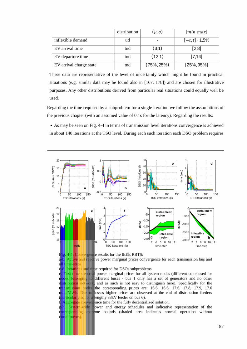
87
distribution (휇,휎) [푚푖푛,푚푎푥]
inflexible demand ud - [−푡, 푡] ∙ 1.5%
EV arrival time tnd (3,1) [2,8]
EV departure time tnd (12,1) [7,14]
EV arrival charge state tnd (75%, 25%) [25%, 95%]
These data are representative of the level of uncertainty which might be found in practical
situations (e.g. similar data may be found also in [167, 178]) and are chosen for illustrative
purposes. Any other distributions derived from particular real situations could equally well be
used.
Regarding the time required by a subproblem for a single iteration we follow the assumptions of
the previous chapter (with an assumed value of 0.1s for the latency). Regarding the results:
As may be seen on Fig. 4-4 in terms of transmission level iterations convergence is achieved
in about 140 iterations at the TSO level. During each such iteration each DSO problem requires
Fig. 4-4: Convergence results for the IEEE RBTS: a-b. Active and reactive power marginal prices convergence for each transmission bus and all time-steps. c-d. Iterations and time required for DSOs subproblems. e. First time-step real power marginal prices for all system nodes (different color used for nodes belonging to different buses - bus 1 only has a set of generators and no other distribution network, and as such is not easy to distinguish here). Specifically for the transmission nodes the corresponding prices are: 16.6, 16.6, 17.6, 17.8, 17.9, 17.6 m.u./MWh. Due to losses higher prices are observed at the end of distribution feeders (particularly so for a lengthy 33kV feeder on bus 6). f. Aggregate convergence time for the fully decentralized solution. g-h. System-wide power and energy schedules and indicative representation of the corresponding extreme bounds (shaded area indicates normal operation without curtailments).
0 50 100 1500
5
10
15
20
pric
e (m
.u./M
Wh)
TSO iterations (k)0 50 100 150
-0.5
0
0.5
1
pric
e (m
.u./M
Var
h)
TSO iterations (k)
a b0 50 100 150
0
2
4
6
8
time
(sec
)
TSO iterations (k)0 50 100 150
0
10
20
30
40
50
DSO
iter
atio
ns (l
)
TSO iterations (k)
dc
1 29415
16
17
18
19
20
node
pric
e (m
.u./M
Wh)
0 50 100 1500
1
2
3
4
time
(min
)
TSO iterations (k)
e f
2 4 6 8 10 12-250
-200
-150
-100
-50
0
time-step
(MW
)
2 4 6 8 10 12-2000
-1500
-1000
-500
0
(MW
h)
time-step
curtailmentregion
curtailmentregion
hginfeasibleregion
infeasibleregion

88
its own number of iterations. Note that the latter as the optimization progresses tend to decrease
thanks to the fact that the TSO level marginal prices stabilize near their optimal values, while
the DSO subproblems have the good initial points provided by the previous TSO level iteration.
The system involves 6 transmission buses and 286 distribution nodes. This means about 7k
power balance and 3.5k line capacity constraints. The constraints number for MO subproblems
would be on the order of 17k. Despite the small size of the system the resulting problem is large.
The results indicate the ability of the proposed scheme to coordinate energy management within
a time frame (in this case less than 4min) acceptable for market applications. As may be seen
the first optimization time step corresponds to a time of high demand with domestic consumption
near its peak. The flexible part of demand is shifted towards later hours. The end result is a rather
flat price and demand profile.
It should be noted that the time to convergence could potentially be improved if instead of a flat
start (i.e. 휆 = 푧 = 0) the simulation was initialized based on a solution of the previous time-
step. More efficient implementations of the used optimization algorithms are also possible than
our current ones (done in MatLab). For the optimization subproblems we used closed-form
solutions if possible, and a primal-dual barrier interior point algorithm. The simulations were run
on an Intel Core i5-2500 3.3Ghz, with 4GB of RAM. The iterative nature of this distributed solution
could allow for improved constraint management heuristics which would remove inequality
constraints that are not expected to become active in the subproblems, thus reducing
computational burden.
4.3.2 Time-wise Scalability
In this section we investigate the impact of look-ahead period in terms of convergence. Based on
the RBTS 6 bus test case a series of simulations were performed with a gradually decreasing
number of time-steps. The results may be seen on Fig. 4-5. The differences in convergence time
and iterations are due to the fact that, as the time-steps number changes, these are effectively
different optimization problems with slightly different solutions. Nevertheless, the changes in
Fig. 4-5: Effect of number of time-steps 푛 on convergence speed.
6 8 10 120
50
100
150
200
nt
TSO
iter
atio
ns (k
)
6 8 10 120
1
2
3
4
nt
time
(min
)

89
time are not significant. The reason is that MO subproblems (which increase in size) are solved
in parallel with the more computationally intensive DSO network subproblems which do not
change in scale (network subproblems for the new time-steps are solved in parallel with the
existing ones). The results indicate that it is possible to increase the number of time-steps without
any negative impact on convergence time.
4.3.3 Network Scalability & Implementation Challenges
In this section we try to gain some insight with respect to scalability in terms of network size.
Unfortunately, data describing a large network including both transmission and distribution were
not available. Therefore, we set up an additional test case based on the IEEE 118 bus network
(base data available on [161]). We retained the transmission level system data as is, and we added
distribution data as copies of the RBTS feeders, e.g. for the 118 system bus 59 (277MW), three
copies of the RBTS bus 3 distribution feeders (85MW) were added with inflexible demand
slightly scaled to give the total of 277MW. This yielded a problem with a total of 1024 distribution
nodes, i.e. about 4 times larger than our base test case. In all other respects (e.g. EV penetration)
the test case was constructed in a similar fashion with the base case. With respect to
decomposition structure: the transmission network was considered as a single area/subproblem;
for buses with large distribution networks, sets of feeders were considered as separate
subproblems (e.g. for the previously mentioned bus 59 three equivalent DSO subproblems were
Fig.4-6: Convergence results for the modified IEEE-118 bus network: a-b. Active and reactive power marginal prices convergence. c. Iterations required for DSO subproblems. d. Aggregate convergence time for the fully decentralized solution.
0 100 2000
20
40
60
pric
e (m
.u./M
Wh)
TSO iterations (k)0 100 200
-1.5
-1
-0.5
0
0.5
1
pric
e (m
.u./M
Var
h)
TSO iterations (k)
a b
0 100 2000
2
4
6
time
(min
)
TSO iterations (k)0 100 200
0
10
20
30
40
50
DS
O it
erat
ions
(l)
TSO iterations (k)
c d

90
created) giving a total of 102 DSOs and 731 MOs. As may be seen on Fig. 4-6 convergence is
achieved in about 5.5 min. This increase in time was due to the slightly increased number of
iterations required at both the transmission and distribution level, and also the larger size of certain
subproblems.
Unavoidably when one moves to even larger systems, as the solution time of the network
subproblems increases, so will the overall convergence time. Based on the presented results the
proposed method appears to be applicable to small or medium sized systems. To determine its
applicability on larger systems further testing is required considering that:
If the communications delays are ignored (i.e. latency is set to 0) then the solution time for
the RBTS-6 and IEEE-118 reduces to about 1 and 2 minutes respectively. Further investigation
into communications structures and modelling expected delays realistically is an important issue,
as is the directly related subject of efficient implementation (in software & hardware) of the
optimization subproblems solvers.
Investigating what are the most efficient distributed solution methods, especially at the
distribution level (potentially exploiting their radial structure), is also an important subject.
Decomposing a very large transmission network into even a small number of areas could
imply a much faster solution of TSO level subproblems, despite an increase in terms of
iterations. However, the inclusion of security constraints and investigating efficient methods for
their decomposition are key issues.
Overall, the presented approach serves as the basic solution concept. Several extensions are
required before a full practical application can be implemented.
4.3.4 Coordination
As pointed out in A1 ED presupposes coordination with UC mechanisms. In addition, the fact
that we cannot have a definitive decision regarding individual microgrid level devices schedules
as part of our overall ED solution, implies that an additional microgrid dispatch (MD) mechanism
is required. The latter should operate at a time resolution much faster than that of ED, and should
be capable satisfying user requirements, handling microgrid network constraints in their full
detail, while following the ED solution as closely as possible. A wide variety of methods have
been proposed in the literature (e.g. [173, 63, 179, 180]) which could be suitably adapted to serve
this purpose.
4.4 Conclusions & Further Questions
The overall energy framework we envision in this work is illustrated in Fig. 4-7. Electricity
markets (through UC and ED) are there to achieve coordination over time and utility
maximization across the whole network; dispatch at the microgrid level will be there to follow
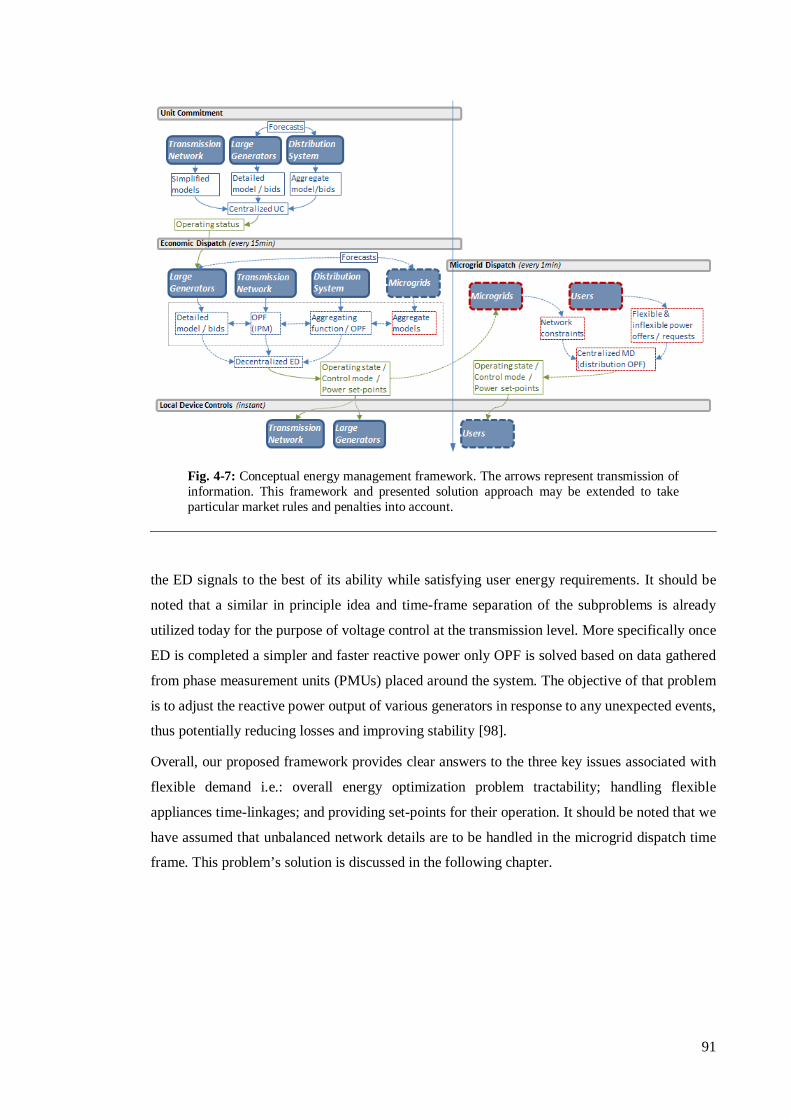
91
the ED signals to the best of its ability while satisfying user energy requirements. It should be
noted that a similar in principle idea and time-frame separation of the subproblems is already
utilized today for the purpose of voltage control at the transmission level. More specifically once
ED is completed a simpler and faster reactive power only OPF is solved based on data gathered
from phase measurement units (PMUs) placed around the system. The objective of that problem
is to adjust the reactive power output of various generators in response to any unexpected events,
thus potentially reducing losses and improving stability [98].
Overall, our proposed framework provides clear answers to the three key issues associated with
flexible demand i.e.: overall energy optimization problem tractability; handling flexible
appliances time-linkages; and providing set-points for their operation. It should be noted that we
have assumed that unbalanced network details are to be handled in the microgrid dispatch time
frame. This problem’s solution is discussed in the following chapter.
Fig. 4-7: Conceptual energy management framework. The arrows represent transmission of information. This framework and presented solution approach may be extended to take particular market rules and penalties into account.

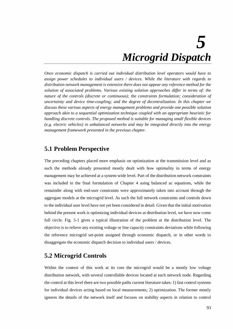
93
5 Microgrid Dispatch
Once economic dispatch is carried out individual distribution level operators would have to assign power schedules to individual users / devices. While the literature with regards to distribution network management is extensive there does not appear any reference method for the solution of associated problems. Various existing solution approaches differ in terms of: the nature of the controls (discrete or continuous); the constraints formulation; consideration of uncertainty and device time-coupling; and the degree of decentralization. In this chapter we discuss these various aspects of energy management problems and provide one possible solution approach akin to a sequential optimization technique coupled with an appropriate heuristic for handling discrete controls. The proposed method is suitable for managing small flexible devices (e.g. electric vehicles) in unbalanced networks and may be integrated directly into the energy management framework presented in the previous chapter.
5.1 Problem Perspective
The preceding chapters placed more emphasis on optimization at the transmission level and as
such the methods already presented mostly dealt with how optimality in terms of energy
management may be achieved at a system-wide level. Part of the distribution network constraints
was included in the final formulation of Chapter 4 using balanced ac equations, while the
remainder along with end-user constraints were approximately taken into account through the
aggregate models at the microgrid level. As such the full network constraints and controls down
to the individual user level have not yet been considered in detail. Given that the initial motivation
behind the present work is optimizing individual devices at distribution level, we have now come
full circle. Fig. 5-1 gives a typical illustration of the problem at the distribution level. The
objective is to relieve any existing voltage or line capacity constraints deviations while following
the reference microgrid set-point assigned through economic dispatch, or in other words to
disaggregate the economic dispatch decision to individual users / devices.
5.2 Microgrid Controls
Within the context of this work at its core the microgrid would be a mostly low voltage
distribution network, with several controllable devices located at each network node. Regarding
the control at this level there are two possible paths current literature takes: 1) fast control systems
for individual devices acting based on local measurements; 2) optimization. The former mostly
ignores the details of the network itself and focuses on stability aspects in relation to control
94
parameters setting of individual devices. The latter either solves complete optimization problems
ahead of time, or uses some continuously executing distributed solution approach. While fast
controls and optimization normally belong to different time frames, depending on how often the
microgrid level optimization subproblem is solved, it could be possible to entirely dispose of the
traditional local measurement based control approach for certain devices and just optimize them
along with the rest of the microgrid. Following is a brief overview of relevant literature along
with a description of the various approaches used.
5.2.1 Pure Control
In terms of fast controls acting on local information (i.e. voltage or frequency measurements),
literature may be further categorized in to two groups. The first deals with frequency or voltage
control in isolated systems, placing particular emphasis on stability. The second relates to the
more traditional transformer tap voltage control approaches in distribution networks.
Several papers discuss various aspects of stability in microgrids (i.e. distribution networks), as
when a significant number of devices respond to a frequency or voltage signal, dynamic stability
may be an issue. For example [181] focuses on the individual frequency and voltage controls of
distributed generation and provides relevant models. An important point however is that the
authors identify the need for a central controller for determining load sharing among DG units
Fig. 5-1: An indicative illustration about what the microgrid dispatch problem is about. The figure illustrates the IEEE-123 nodes distribution test feeder which in the context of this work we consider as a microgrid. Numbered items correspond to system nodes, while circles correspond to transformers or voltage regulators. Each node may have any number of devices connected in any possible configuration. The colour-map is associated with voltage (large deviations from 1p.u. in red, closer to 1 p.u. green). This corresponds to a case with high EV penetration, assuming the latter are left uncontrolled. The network is connected to transmission through node 149 (located bottom left).
95
and maintaining power quality and required stability margins, i.e. the equivalent of the microgrid
dispatch mechanism. Reference [182] follows similar lines focusing on individual local controls.
In a more traditional context, where only transformer tap controls are available, reference [183]
proposes a solution which is based on an approximate network model. The underlying principle
is that following various transformer actions, measurements taken can be used to estimate the
Thevenin equivalent of the low-voltage side circuit. Subsequently that model could be used to
determine the tap operations. Note that this paper does not appear to necessarily refer to
distribution level transformers only. A similar in principle approach is also proposed in [184] for
controlling photovoltaic generators in order to prevent overvoltage, as well as in [185]. While
these approaches are relevant to traditional tap-changer control practices, they do not quite fit in
coordinated energy management schemes, which could instead concurrently optimize all involved
control variables based on a predetermined system model.
While the above hardly cover published work on these areas, they are representative enough to
make two basic points. First, certain traditional methods to voltage control, while important by
today’s standards, could be irrelevant in a ‘smarter’ network where optimality is pursued through
device coordination. Second, especially when it comes to managing demand, it is very important
in terms of use of available controls to differentiate between optimal energy management and
system support in contingency cases. The former relates to the procurement of requested energy
and sufficient control margins (i.e. operating the device at such a power set-point that its output
may be adjusted up or down as necessary in the future); the latter makes use of the aforementioned
control margins by responding to local signals (e.g. frequency) which may exhibit very fast
changes. It should be clear that these two functions have to be served in two significantly different
time scales.
5.2.2 Centralized Energy Management – Network Unconstrained
A significant number of papers look into the optimal scheduling of flexible demand devices (most
commonly electric vehicles) without any consideration of the ac network constrains, other than
possibly a capacity limit on the aggregate demand. This yields a rather simple, yet still quite large
optimization problem, which due to the lack of network limitations, is amenable to a wide range
of algorithms and solution approaches.
Reference [186] proposes the idea of defining a preferred operating point for individual EVs. This
may be determined through a variety of simplified ‘smart’ algorithms (which may be actually
suboptimal), or through a continuous multi-period (profit maximizing) optimization carried out
by the aggregator. A total of 3 different formulations are presented that seem to prioritize charging
either based on expected prices, or state of charge, or expected demand. Overall the need or actual
benefit for all these proposed formulations is not quite clear.

96
Reference [187] makes an interesting contribution by considering both scheduling and dispatch.
A linear programming based approach is proposed for the scheduling time frame and a heuristic
for the dispatch. Note however that it does not consider system-wide coordination - it rather uses
price forecasts. In terms of dispatch a simple ranking scheme is used which assigns demand to
slots by looking only at EVs which have already arrived. The proposed heuristic is capable of
handling both continuous and discrete variables.
Reference [188] again supports the hierarchical control concept of the microgrid and formulates
an optimization problem that includes bidding from demand. However, in many respects the
proposed approach appears to be oversimplified, given that once more a simple priority list is
used for scheduling individual devices. A ranking heuristic to determine demand scheduling in
real-time applications is also proposed in [189]. This heuristic assigns quadratic utility functions
to individual devices, yielding a single time-step quadratic programming problem.
Reference [190] considers a variety of both continuous and integer controls in a multi-period
formulation using point-estimates for uncertain quantities and a heuristic to determine allocation
of reserves. The exact time frame of application of this control and its connection with the rest of
the power system is not clear. A similar approach is followed in [191] which proposes a multi-
period mixed integer formulation for managing day-ahead scheduling of a smart grid, using a
particle swarm optimization method for its solution. A mixed integer linear programming
formulation is also proposed in [192] to schedule EVs at the aggregator level. The objective
function includes a penalty for unserved demand, the cost of energy to the aggregator and a term
for losses or operational costs due to energy exchanges within the network. The time-frame of
application is yet again not clear.
Reference [193] for the purpose of managing EVs in grid-connected microgrids uses continuous
variables for individual EV states, within a multi-period deterministic formulation. Again this is
of limited practical value as it does not consider distribution constraints and coordination with the
markets. A similar model is presented for cases where the microgrid is islanded and load shedding
is required, which assigns an energy value to each EV based on fuzzy rules and their current state
of charge. A more refined continuous optimization approach appears in [12]. A lognormal
distribution is assumed to adequately describe individual vehicle daily energy requirements.
Based on the central limit theorem the paper suggests that for a large number of vehicles the
charging requirements may be expected to follow a normal distribution. The objective of the
derived quadratic programming problem is minimization of demand variance over a day, with a
control variable being the percentage of EVs which would start charging at a specific hour.
However, the paper does not consider any stochastic variables other than energy requirements
themselves and the approach does not appear to be easily extensible.

97
Reference [194] proposes a rolling horizon optimization formulation for EVs. This involves
typical charging constraints with the inclusion of battery lifetime penalties in the objective
function. No network constraints are included and costs are assumed to follow a quadratic
function. While the proposed approach appears to be of little interest, the paper identifies potential
tractability issues and the difficulties associated with management of uncertainty.
Reference [195] presents an algorithm to facilitate charging subject to given scheduling
obligations. First the authors solve a 5 day ahead scheduling problem to determine demand
requirements. To reduce the dimensions of the problem vehicles are clustered into fleets. The
solution of this problem generates prices for each of the EV clusters. When a new vehicle plugs-
in its charging is scheduled based on these prices. However, it should be noted that the scheduling
obligations appear in the form of a capacity cap, rather than actual market penalties.
In [196] a method is proposed for coordinated voltage control in a distribution network that
proposes a quite complex heuristic based on a ‘beliefs’ and ‘intentions’ agent based framework.
This involves the exchange of a series of voltage measurement values between closely located
agents, which eventually allow each agent to form an estimate of the network state, and
subsequently make a control decision. The overall approach appears to be unnecessarily
complicated.
While there are several different methods appearing to deal with EV energy management, none
of them is essentially complete. The reason for this is not only due to the fact that they do not take
into account network constraints, but they also do not consider coordination with the transmission
level and do not specify their time-frame of application. As such this body of work does not appear
to lead to any definitive direction towards the solution of the microgrid level optimization and
control problem.
5.2.3 Centralized Energy Management – Network Constrained
A much more challenging optimization problem arises when network constraints are actually
taken into account. As already discussed in Chapter 2 of this work, there is a variety of options in
terms of how these constraints are represented. This is reflected in relevant literature which adds
to the existing exact mathematical models a number of arbitrary, rough approximations.
Reference [197] once again indicates the requirement for a hierarchical control structure for the
microgrid with the slowest of those controls optimizing active and reactive power set-points. This
paper focuses on storage device control which may be assumed to operate in a continuous manner,
using standard non-linear power flow equations, with the objective being the minimization of
energy imports. The paper uses dynamic programming to solve the corresponding deterministic
multi-period optimization problem.

98
In [198] an energy management approach is proposed where the distribution system operator
attempts to determine the right prices for the system through the solution of a single-time-step
optimization problem. It is assumed however that the DSO can predict the consumers’ response
to the given price signals. Given the uncertainty involved at this level and the fact that this is
actually a scheme involving communications between individual users and the system operator,
this approach appears to be of limited practical interest.
In [199] a real time optimal power flow approach is suggested for managing renewable generation
in a medium voltage distribution network. From a theoretical perspective there is nothing
particularly new here, however an interesting point is the use of a last-in-first-out logic in
determining the objective function for the optimal power flow problem. This is a continuous
variables optimization approach, with standard balanced ac power flow constraints. A variant of
this scheme appears in [200] which instead of non-linear programming uses a constraint
satisfaction approach. Beyond the fact that this alternative approach handles integer controls only,
there do not appear to be any clear benefits to it. The authors improve upon this scheme in [201]
by extending the formulation to a multi-period one but without any specific mention about how
uncertainty is modelled.
In [202] a centralized losses minimization problem is formulated for EV scheduling, and proceeds
to compare the results of a deterministic quadratic and a stochastic formulation. The proposed
approaches are suitable for handling continuous variables only and appear to include an
approximate representation of network constraints. Uncertainty is considered in the form of a
predetermined number of scenarios without however providing sufficient justification for this
particular choice. For the stochastic formulation a dynamic programming technique is used but
no specific information regarding solution times is provided.
Reference [203] proposes a continuous variables formulation, using approximate convex network
models, which minimizes demand variance and in turn losses. The approach appears to be of
limited practical value as it is unclear how it could be extended to overall cost minimization. An
approximate formulation is also used in [180] in the form of a current-based DC approximate
formulation for the system including voltage drop and phase unbalance. The latter is considered
in terms of phase load deviation from the average node load, rather than in percentage of the
negative sequence voltage component. This approach gives a linear programming problem
however the proposed model, while accurate perhaps for limited length networks, is unlikely to
prove accurate for larger cases.
Reference [204] proposes an algorithm for optimizing EV charging in low voltage networks so
that system voltage and thermal constraints are taken into account. This iterative centralized
algorithm is based on a linearized unbalanced load flow. The linearization uses sensitivities which
are calculated based on the network solution prior to the connection of EVs. The selection of
99
objective function is somewhat peculiar, as it tries to maximize total power delivered within a
given time period. An interesting point to note is that the paper proposes state of charge based
utility functions in order to balance out the fact that demand closer to the feeder will tend to be
satisfied faster due to lower losses. A similar in principle approach had also been used the authors
in [205] and it was compared with a basic distributed control scheme where each vehicle manages
its energy consumption based on local voltage and conductor capacity limitations. However, the
details about how the latter works and considerations regarding its stability were not adequately
discussed.
Reference [206] proposes a deterministic mixed integer linear programming formulation for
scheduling EV charging at the distribution level in a day-ahead context, assuming fixed energy
prices for each time slot. However, it uses a DC power flow formulation – presumably solving
individually all three phases – which can have significant errors. To counter this error, the authors
added an arbitrary parameter in the line capacity constraints to ensure the results were on the safe
side. The latter, while not a bad idea, appears to be poorly executed. It is of interest though that a
DC approximation is also used in [171], as part of the proposed solution for the same problem. In
this case a continuous multi-period formulation is proposed, assuming exact forecasts regarding
energy prices at the transmission level and any demand at the distribution network level.
Finally, reference [207] proposes a simple algorithm for determining power set-points for
distributed generation based on calculated sensitivities. However, it is not particularly clear how
well the proposed scheme performs in terms of coordination of demand of several different
generators. This approach accounts for both continuous and discrete controls, considering a
linearized version of the power flow equations.
While the mathematics behind the various approaches mentioned above are certainly more
interesting compared to the network unconstrained approaches, overall there is nothing conclusive
about the current literature. The limitations of individual methods in terms of problem scale are
not clear, hence there is also no clear indication with regards to what formulation should be ideally
used. It is also unclear what the practical challenges are expected to be, and the time-frame of
application for these solutions is typically not specified.
5.2.4 Decentralized Perspective
In terms of energy management at the distribution level decentralized methods have recently
become quite popular. The vast majority of relevant papers however uses simplified network
unconstrained forms of the problem. In [208] a basic distributed agent-based power management
scheme is proposed where each agent optimizes his own operation assuming a fixed grid energy
price. The mechanism for agent cooperation is not particularly sophisticated however and does
not seem suitable for problems of larger scale, or in cases where a mathematically optimal solution
100
is of interest. Reference [209] proposes an auction mechanism based on a so-called symmetric
assignment algorithm for managing energy within a microgrid. The overall model is however
quite simplistic, takes no account of network constraints or time-linkages, and there does not
appear to be a way to extend it to include these considerations.
In [210] a seemingly decentralized voltage control by distributed generators scheme is proposed.
The scheme is based on linearized power flow equations and the simple reasoning that the
generator with the highest sensitivity should respond first. The scheme involves each generator
estimating locally its sensitivity, broadcasting this information to a central agent, who responds
with an estimate of the amount of reactive power required by each generator.
Dynamic programming (DP) as a means for stochastic control in the smart grid was presented in
quite general terms in [211]. A more specific relevant approach is proposed in [212] where the
authors use two distributed optimization heuristics, both with dynamic programming origins, for
managing flexible users. The first heuristic is quite similar to LR where user subproblems are
simply solved via dynamic programming. The second method is based on a DP variant called Q-
learning approach, which allows to a certain degree the combination of stochastic characteristics
of different users. Both approaches seem to have comparable convergence characteristics and are
shown to be close to optimal. In any case, the Bellman equation seems to provide a basis for
decomposing the problem in terms of time.
In [213] a bi-level programming structure for solving a single time-step network unconstrained
energy management problem is proposed, where the microgrid aggregator sends demand
information to a central production unit and receives back price information. The mathematical
background and the actual value of the proposed scheme are rather unclear.
Proximal decomposition methods similar to the one used in a previous chapter are also quite
popular in the EV management problem. A variant is proposed in [214] where each player has
knowledge of the utility function and the power schedules of other players. Subsequently he
optimizes his potential benefits (including the proximal term) with the assumption that other
players’ schedules remain fixed. This algorithm is proved to converge to a Nash equilibrium for
a suitable selection of the proximal term penalty factor. Quite a similar approach is proposed in
[215]. For a test case with 10 users / subproblems convergence is achieved within 20-30 iterations.
Another proximal method variant used in [216]. This reference also involves a detailed analysis
on the marginal price signal used in this scheme, but the point behind this analysis is not entirely
clear. Note that the methods in the above papers handle deterministic problems with continuous
variables only, and have not been proven to work with the full network constraints.
Reference [217] instead of a proximal term, penalizes the deviation of an EV charging strategy
for the average behaviour of the EV fleet. This approach is proven to converge to a Nash
equilibrium. However, it is not clear how devices of a different type could be incorporated into
101
this approach and as such its use is rather limited. Some latency values are also mentioned in the
experiments carried out as a part of this work (60푚푠 between aggregator and EV, 500푚푠 between
aggregator and agent at HV/MV substation). However, the related communications infrastructure
is not explained in detail and as a consequence it is not clear how close in practice these values
are. A similar approach is used in [218]. It should also be noted that this algorithm does not
necessarily fully converge at a globally optimal point in the case where the EV population is
heterogenous (i.e. different charging times and characteristics among various vehicles). This is a
disadvantage that the previously mentioned methods do not have and as such this algorithm is of
no further interest. Despite this fact a similar approach is also used in [219].
Another variant of the proximal penalty schemes may be found in [220]. In that paper individual
devices are allowed to reside in discrete states. In their optimization subproblems a penalty term
is introduced which actually penalizes big scheduling changes from one iteration to the next. For
a set of 100 users the algorithm is shown to converge within a few tens of iterations. In principle
this algorithm can handle both continuous and discrete variables but does not appear to take into
account any network constraints or any associated uncertainties. As may be expected this
algorithm is a heuristic and care should be taken when selecting the penalty factor as it may yield
results far from the optimum.
Reference [221] proposes an ADMM based solution to the EV charging problem. While charging
power is initially assumed to take discrete values, all discrete variables are relaxed into
continuous. Furthermore, a utility function dependent on state of charge and time to go is used.
Regarding convergence, it is assumed that only a certain number of iterations are allowed. It is of
note that the proposed structure involves a series of sub-aggregators (MOs) and one central
aggregator (DSO) essentially for the purpose of managing the discrete nature of the controls.
Overall what is proposed is a method which approximately considers discrete controls through
the aggregators themselves but does not consider network constraints and the various sources of
uncertainty. Note that the solution is decentralized only as far as the continuous relaxation is
concerned. The ADMM approach is also used in [222], albeit in a much simpler problem
formulation which involves continuous controls only. Note that this paper reports very fast
convergence (i.e. within 10-20 iterations), but this is probably a direct result of the assumed highly
convex energy cost function. An even more simplified formulation is used in [223], this time
solved via LR. In terms of network constraints, the paper considers only a single capacity
constraint, and only expected energy prices are used which are not affected by the EV scheduling.
Reference [224] proposes an LR based scheme for coordinating devices schedules where the
distribution system operator broadcasts and updates prices. The proposed method solves a
deterministic problem, is able to handle continuous variables only, and does not appear to include
any network constraints. The authors additionally consider the effect of lost messages between

102
the residential smart meters and the operator, showing that the algorithm still converges in near
optimal solutions.
In [225] a consensus based algorithm is proposed for EV charging. This approach however is
applicable to continuous variables problems only and cannot possibly take into account any
network constraints. In terms of papers that do take into account network constraints reference
[226] uses a semi-definite programming formulation coupled with a Lagrangian Relaxation based
scheme. This is a single-time step optimization focusing on controlling voltage through any
available distributed energy sources. This approach is in principle similar to [130], which however
considers the full 3-phase unbalanced power flow.
5.2.5 Concluding Remarks
Overall, with respect to the developing trend of using decentralized approaches and a possible
dilemma between which type of method should be preferred, there are two points to be made.
First, determining operating set-points for individual devices presupposes the knowledge of both
the network and individual device status. It would be unrealistic to assume that individual users
will be given access to full information of the distribution network. As such for both centralized
and decentralized solutions, all relevant information will always go through one central entity (i.e.
the DSO or MO) who could respectively provide directly the solution or coordinate individual
responses (e.g. by broadcasting suitable price signals). As such there is no apparent benefit in
terms of reliability if a decentralized approach is selected. At the same time privacy of energy use
on the individual user level when usage information is measured is purely an illusion. Second, an
important difference between a centralized and a decentralized approach is that the former would
require only one round of communications (one for receiving user requirements / measurements
and one for broadcasting results), while the latter would require one round for each iteration until
convergence. As such a decentralized approach would imply much larger requirements in terms
of communications.
It is a fact that distribution networks have never been optimized in real-time as transmission
typically is, and microgrids are a relatively new concept. As such there is no reference problem
formulation. In turn, given the lack of clear problem definition and identification of its most
important parameters, as a research area, distribution and the concept of smart grids provide a
fertile ground for the application of a wide range of methods. However, their supporting problem
formulation, and as a consequence some of the methods themselves, can be of little practical
value.
In terms of decentralized methods, it is worth pointing out that, only a very limited number of
papers take into account network constraints (e.g. [130]) and fewer still consider the discrete
nature of certain controls [173]. Achieving optimality in this sort of problem in a decentralized
103
fashion is not easily accomplished. In addition, with respect to approximate continuously
executing decentralized energy management methods, it is unclear how they would work along
with any faster individual device controls intended to cope with contingencies (related e.g. to
frequency or voltage) – unless of course there are no such controls. Based also on the
considerations of the previous paragraph it is reasonable to assume that at the microgrid level, as
long as the scale of the problem is manageable, a centralized solution would probably be
preferable. Consequently, in the following we focus on centralized optimization approaches
which should be able to incorporate discrete control decisions.
5.3 Utility Functions for Demand
In the general case, both the value of the high penalty typically set for not serving the demand and
the actual utility gained from supplying it, are hard to define clearly. The potential availability of
a large number of similar controllable devices in a small network implies that if losses are not
taken into account any relevant optimization formulation can have an infinite number of possible
solutions. On the other hand, if losses are considered, end node customers will always be the last
ones to be served and the first ones to be curtailed if necessary. The idea of using appropriately
selected utility functions to induce a unique solution or a fair allocation of resources, or simply
allow the implementation of certain control or optimization techniques has been discussed in
several papers.
One such class of papers is based on similar concepts used in telecommunications. Reference
[227] proposes a logarithmic function of the form 푢 = 푤 log(푃) where 푤 represents the user’s
willingness to pay. Using such a utility function is said to lead to proportional fairness among
network users, i.e. a Nash equilibrium where the energy each user consumes at equilibrium is
proportional to 푤. The reasoning behind this approach is based on rate control applied to
communication networks as proposed in [228]. This logarithmic function appears again in [229]
and also in [230]. In the latter the decentralized approach is assumed to run continuously and the
schedule updates are directly applied, rather than applied once after the algorithm’s convergence.
In terms of more centralized approaches [205] proposes scaling of EV utility functions based on
their state of charge so that it is ensured that end-node customers get served. A much more
elaborate utility function is used in [231]. A quadratic function for EVs is used, which depends
on the state-of-charge and every other parameter possibly related to the vehicle battery charging
requirements.
A common characteristic of all the above papers is that they use single time-step problem
formulations. In that case the modified utility functions could allow to take into account in an
indirect approximate way the requirements of demand over time. An additional benefit of course
could be a strongly convex objective function for the overall problem, which would imply

104
improved convergence for any applied distributed solutions. It should be noted that within the
context of a multi-period formulation the value of modified utility functions could be hard to
justify, especially when a solution that satisfies all user requirements exists.
5.4 Problem Formulation
Based on the considerations of the previous chapters and our developed framework, in this chapter
we formulate and solve the microgrid dispatch problem based on the following assumptions:
A1. Dispatch at the microgrid/distribution level has the objective to assign power set-points to
individual devices while satisfying user requirements, and following as close as possible the
microgrid-system power exchange levels promised in the last economic dispatch solution. As
such the time available for solving the microgrid dispatch problem should be less than the time-
resolution of solving the economic dispatch problem.
A2. The microgrid operator utilizes sufficiently accurate models in terms of aggregate power for
its participation in energy markets. As such possible deviations from the market position in
future time-steps need not be considered within the microgrid dispatch problem.
A3. We opt to use the three-phase reference frame assuming that in terms of energy management
any return (neutral conductor / earth) currents are not of interest. As such Kron’s reduction is
carried out where applicable.
A4. The problem of network reconfiguration, if it were of interest for a given network, would
be solved on a different time scale. The reasoning is that this is a problem of significant
complexity involving also protection considerations. At the same time, it is unlikely that the
network operator would allow a significant number of switching actions during a day.
A5. Rather than formulating a multi-period MD problem a single time-step formulation is used
on the assumption that the impact of the device time-linkage characteristics has been
adequately considered through the aggregate models used in during ED. As such following the
microgrid aggregate set-points provided by the ED solution is sufficient. To ensure that end-
node users are served in all possible cases, we scale their utility functions based on their state-
of-charge or electrical distance.
The downside of assumption A5 would be slightly increased losses compared to the case where
a multi-period formulation would be used. However, the computational burden of such
approaches can be significant. As such our overall optimization problem may be written as:
min퐬,퐬
⎩⎪⎨
⎪⎧ 푢 { }
∈
+ 푐 |푃 − 푃 | ∶
퐶퐶 ( )퐶 ( )
푖푓 푑푒푣푖푐푒 푖 푖푠 푖푛푓푙푒푥푖푏푙푒푖푓 푑푒푣푖푐푒 푖 푖푠 푓푙푒푥푖푏푙푒
∈ ⎭⎪⎬
⎪⎫
( 5–1)

105
퐶 =
⎩⎪⎨
⎪⎧풆 푑푖푎푔{∠퐕}퐜 퐈 = 퐈
퐈 = 퐘 (퐬 )풆 퐕 퐾푖푟푐ℎℎ표푓푓′푠 푙푎푤푠
|퐜 퐕| ≤ ퟏ 푛푒푡푤표푟푘 푐푎푝푎푐푖푡푦0.95 ≤ |퐕| ≤ 1.05 푣표푙푡푎푔푒 푎푚푝푙푖푡푢푑푒|풄 퐕| ≤ 0.02|풄 퐕| 푣표푙푡푎푔푒 푢푛푏푎푙푎푛푐푒⎭
⎪⎬
⎪⎫
( 5–2)
퐶 { } =푢 { } = 푐 { } 1− 퐬( )
퐈( ) = 퐬( , )푒 푐 { } + 푐 { }|퐕| + 푐 { }|퐕|퐬( ) ∈ {0,1}
( 5–3)
퐶 { } =
⎩⎪⎨
⎪⎧푢 { } = 푐 { }퐬( , )|퐕|퐈( ) = 퐬( ) + 푗퐬( )
푐 { }|퐕| ≤ 퐬( ) ≤ 푐 { }|퐕|푐 { }|퐕| ≤ 퐬( ) ≤ 푐 { }|퐕| ⎭
⎪⎬
⎪⎫
( 5–4)
Where:
푁 Set of 푛 devices / users currently connected in system.
푁 Set of the 푛 nodes in the system.
퐬 Device / user operating status vector.
퐬 Voltage regulators tap position.
푢 Cost function (negative utility) for individual device / user power or energy requirements.
푐 Penalty associated with deviation from market schedule.
푃 Power injection of the microgrid to the power system.
푃 Power injection of the microgrid to the power system as a result of the MO participation in energy markets (i.e. unit commitment, economic dispatch mechanisms). Note that with 푃 = 0 and 푐 ≪ VOLL, the above is reduced to a standard loss / power minimization problem.
퐘 Nodal admittance matrix: this is a function of 퐬 .
퐕 Complex node voltages 푛 × 1 vector in the a-b-c reference frame. The bounds in this case are set at ±5% which is typical for medium voltage networks. For low voltage networks these may be further increased to ±10%. Voltage is expressed in rectangular coordinates, i.e. 퐕 = 퐕 + 푗퐕 .
퐈 Complex current injection 푛 × 1vector of devices at a reference frame aligned to the voltage angle of the device.
퐜 Matrix 푛 × 푛 associating current injections with nodes, e.g. 퐜 ( , ) = 퐼 { } if the single phase device k is connected at node j and 0 otherwise; where 퐼 { } the nominal current of the device.
퐜 Matrix 3(푛 − 1) × 푛 associating node voltages with branch flows; each equation is normalized by the corresponding current limit.
퐜 , 퐜 Matrix 푛 × 푛 converting a-b-c voltages to corresponding zero and positive sequence components.
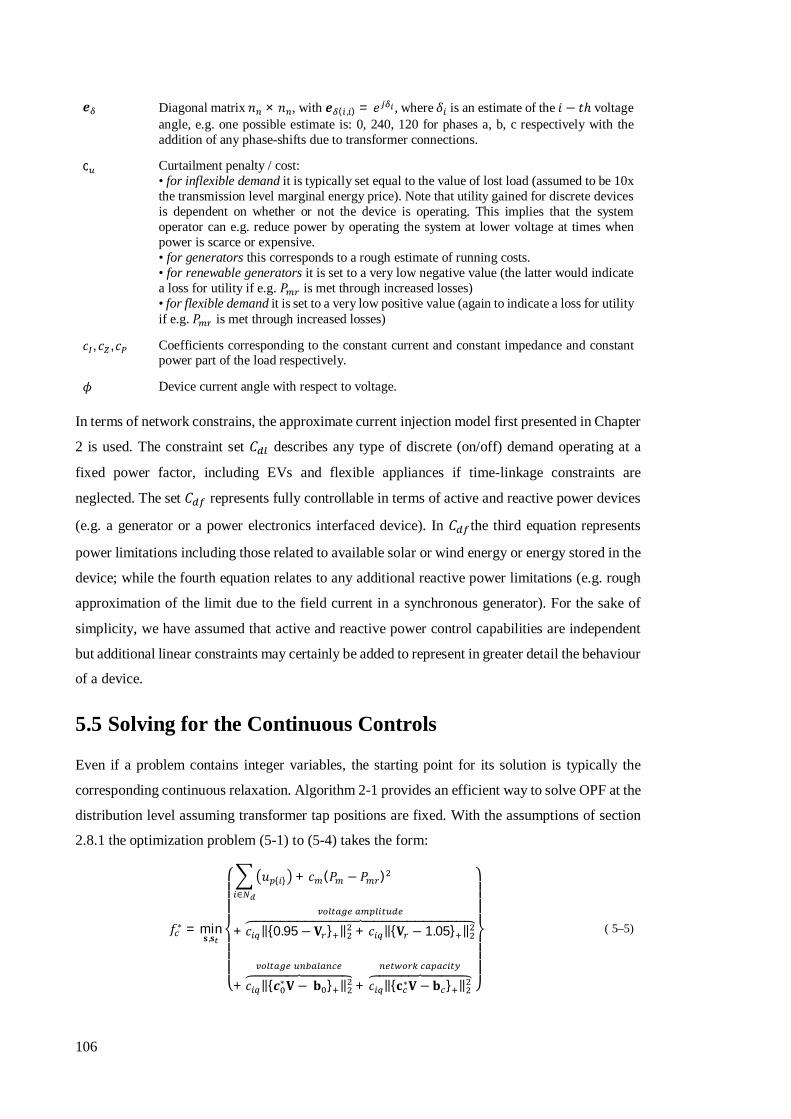
106
풆 Diagonal matrix 푛 × 푛 , with 풆 ( , ) = 푒 , where 훿 is an estimate of the 푖 − 푡ℎ voltage angle, e.g. one possible estimate is: 0, 240, 120 for phases a, b, c respectively with the addition of any phase-shifts due to transformer connections.
c Curtailment penalty / cost: • for inflexible demand it is typically set equal to the value of lost load (assumed to be 10x the transmission level marginal energy price). Note that utility gained for discrete devices is dependent on whether or not the device is operating. This implies that the system operator can e.g. reduce power by operating the system at lower voltage at times when power is scarce or expensive. • for generators this corresponds to a rough estimate of running costs. • for renewable generators it is set to a very low negative value (the latter would indicate a loss for utility if e.g. 푃 is met through increased losses) • for flexible demand it is set to a very low positive value (again to indicate a loss for utility if e.g. 푃 is met through increased losses)
푐 , 푐 , 푐 Coefficients corresponding to the constant current and constant impedance and constant power part of the load respectively.
휙 Device current angle with respect to voltage.
In terms of network constrains, the approximate current injection model first presented in Chapter
2 is used. The constraint set 퐶 describes any type of discrete (on/off) demand operating at a
fixed power factor, including EVs and flexible appliances if time-linkage constraints are
neglected. The set 퐶 represents fully controllable in terms of active and reactive power devices
(e.g. a generator or a power electronics interfaced device). In 퐶 the third equation represents
power limitations including those related to available solar or wind energy or energy stored in the
device; while the fourth equation relates to any additional reactive power limitations (e.g. rough
approximation of the limit due to the field current in a synchronous generator). For the sake of
simplicity, we have assumed that active and reactive power control capabilities are independent
but additional linear constraints may certainly be added to represent in greater detail the behaviour
of a device.
5.5 Solving for the Continuous Controls
Even if a problem contains integer variables, the starting point for its solution is typically the
corresponding continuous relaxation. Algorithm 2-1 provides an efficient way to solve OPF at the
distribution level assuming transformer tap positions are fixed. With the assumptions of section
2.8.1 the optimization problem (5-1) to (5-4) takes the form:
푓∗ = min퐬,퐬
⎩⎪⎪⎪⎨
⎪⎪⎪⎧ 푢 { }
∈
+ 푐 (푃 − 푃 )
+ 푐 ‖{0.95−퐕 } ‖ + 푐 ‖{퐕 − 1.05} ‖
+ 푐 ‖{풄∗퐕 − 퐛 } ‖
+ 푐 ‖{퐜∗퐕 − 퐛 } ‖
⎭⎪⎪⎪⎬
⎪⎪⎪⎫
( 5–5)
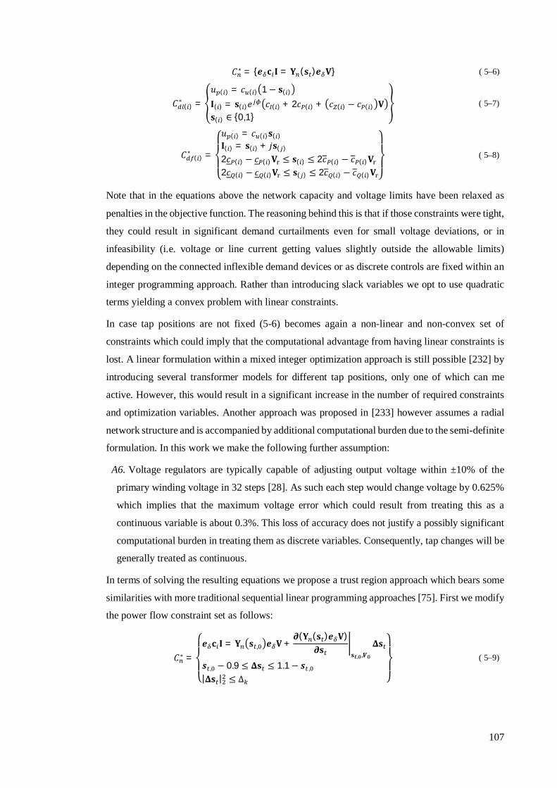
107
퐶∗ = {풆 퐜 퐈 = 퐘 (퐬 )풆 퐕} ( 5–6)
퐶 ( )∗ =
푢 ( ) = 푐 ( ) 1− 퐬( )
퐈( ) = 퐬( )푒 푐 ( ) + 2푐 ( ) + 푐 ( ) − 푐 ( ) 퐕퐬( ) ∈ {0,1}
( 5–7)
퐶 ( )∗ =
⎩⎪⎨
⎪⎧푢 ( ) = 푐 ( )퐬( )퐈( ) = 퐬( ) + 푗퐬( )
2푐 ( ) − 푐 ( )퐕 ≤ 퐬( ) ≤ 2푐 ( ) − 푐 ( )퐕2푐 ( ) − 푐 ( )퐕 ≤ 퐬( ) ≤ 2푐 ( ) − 푐 ( )퐕 ⎭
⎪⎬
⎪⎫
( 5–8)
Note that in the equations above the network capacity and voltage limits have been relaxed as
penalties in the objective function. The reasoning behind this is that if those constraints were tight,
they could result in significant demand curtailments even for small voltage deviations, or in
infeasibility (i.e. voltage or line current getting values slightly outside the allowable limits)
depending on the connected inflexible demand devices or as discrete controls are fixed within an
integer programming approach. Rather than introducing slack variables we opt to use quadratic
terms yielding a convex problem with linear constraints.
In case tap positions are not fixed (5-6) becomes again a non-linear and non-convex set of
constraints which could imply that the computational advantage from having linear constraints is
lost. A linear formulation within a mixed integer optimization approach is still possible [232] by
introducing several transformer models for different tap positions, only one of which can me
active. However, this would result in a significant increase in the number of required constraints
and optimization variables. Another approach was proposed in [233] however assumes a radial
network structure and is accompanied by additional computational burden due to the semi-definite
formulation. In this work we make the following further assumption:
A6. Voltage regulators are typically capable of adjusting output voltage within ±10% of the
primary winding voltage in 32 steps [28]. As such each step would change voltage by 0.625%
which implies that the maximum voltage error which could result from treating this as a
continuous variable is about 0.3%. This loss of accuracy does not justify a possibly significant
computational burden in treating them as discrete variables. Consequently, tap changes will be
generally treated as continuous.
In terms of solving the resulting equations we propose a trust region approach which bears some
similarities with more traditional sequential linear programming approaches [75]. First we modify
the power flow constraint set as follows:
퐶∗ =
⎩⎪⎨
⎪⎧풆 퐜 퐈 = 퐘 퐬 , 풆 퐕+
흏(퐘 (퐬 )풆 퐕)흏퐬 퐬 , ,푽
횫퐬
풔 , − 0.9 ≤ 횫퐬 ≤ 1.1− 풔 ,|횫퐬 | ≤ Δ ⎭
⎪⎬
⎪⎫
( 5–9)

108
Where 횫퐬 = 퐬 − 퐬 , . This linear approximation especially in terms of minimization of losses
will only be accurate for a limited range of tap changes around 퐬 , , as such a trust-region has to
be established. This is the role of the third constraint. Our solution algorithm 2-1 is then modified
as follows:
Algorithm 5-1: Trust-region based OPF
0. Initialization: Set 푒 to best available estimate of voltage angles and taps position s ; and set 푐 = 10 . Solve (5-5) with fixed tap values subject to (5-6) to (5-8). Let this most current OPF solution be denoted as 푃 . 1. Tap update: Update 푒 from 푃 and solve (5-5) subject to (5-7) to (5-9). Let this solution be denoted as 푃 . 2. Convergence check: If |Δs | ≤ 휖 then the algorithm has converged, else go to next step. 3. Tap update check: Update 푒 and s from 푃 ; solve an ac power flow and estimate the objective function value of (5-5). Let this solution be denoted as 푃 . If 푓∗| <푓∗| then set 푃 = 푃 and go to step 1, else go to step 4. 4. Trust-region update: Set Δ = 0.5 min{max|Δs | }. 5. Reference-frame update: If for 푃 푚푎푥{푖푚푎푔(V)} > 휖 , update 푒 from 푃 and update 푃 (similar to O1-step 2). Go back to step 1.
The reasoning behind applying the trust-region approach to the approximate formulation, rather
than using an exact linearization, is that this significantly simplifies any considerations related to
the trust-region itself (i.e. the trust region needs to be defined based only on similarly scaled tap
change variables). A notable advantage is also that issues related to feasibility in terms of voltage
constraints, as e.g. in [94], are not a concern. To test the method’s performance, we use the same
IEEE distribution feeders test cases of Chapter 2, with the only difference being that taps are now
optimized. The results are summarized in the following table.
Table 5-1: Performance of algorithm 5-1 and tap-changers approximation errors: (voltage bounds ±10; tap are optimized for power minimization) Solution
time (sec) Iterations Max. tap
rounding error Power
reduction IEEE-13 0.32 5 0.0029 -3.78% IEEE-34 0.89 4 0.0038 -5.16% IEEE-37 0.49 4 0.0030 -8.03% IEEE-123 2.62 16 0.0031 -4.42%
The following points are of interest:
• Given that our formulation includes constant impedance devices the total demand is actually
reduced compared to the base case through the action of the tap-changers which reduce voltage
at the load (losses do not significantly vary and remain slightly above 3%).
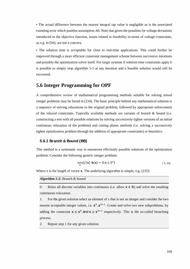
109
• The actual difference between the nearest integral tap value is negligible as is the associated
rounding error which justifies assumption A6. Note that given the penalties for voltage deviations
introduced in the objective function, issues related to feasibility in terms of voltage constraints,
as e.g. in [94], are not a concern.
• The solution time is acceptable for close to real-time applications. This could further be
improved through a more efficient constraint management scheme between successive iterations
and possibly the optimization solver itself. For larger systems if solution time constraints apply it
is possible to simply stop algorithm 5-1 at any iteration and a feasible solution would still be
recovered.
5.6 Integer Programming for OPF
A comprehensive review of mathematical programming methods suitable for solving mixed
integer problems may be found in [234]. The basic principle behind any mathematical solution is
a sequence of solving relaxations to the original problem, followed by appropriate enforcement
of the relaxed constraints. Typically available methods are variants of branch & bound (i.e.
constructing a tree with all possible solutions by solving successively tighter versions of an initial
continuous relaxation of the problem) and cutting planes methods (i.e. solving a successively
tighter optimization problem through the addition of appropriate constraints) or heuristics.
5.6.1 Branch & Bound (BB)
This method is a systematic way to enumerate efficiently possible solutions of the optimization
problem. Consider the following generic integer problem:
푚푖푛퐱
{푓(퐱):퐡(퐱) = 0,퐱 ∈ ℤ } ( 5–10)
Where n is the length of vector x. The underlying algorithm is simple, e.g. [235]:
Algorithm 5-2: Branch & bound
0. Relax all discrete variables into continuous (i.e. allow 퐱 ∈ ℝ) and solve the resulting
continuous relaxation.
1. For the given solution select an element of x that is not an integer and consider the two
nearest acceptable integer values, i.e. 퐱 ,퐱 . Create and solve two new subproblems, by
adding the constraint 퐱 ≤ 퐱 and 퐱 ≥ 퐱 respectively. This is the so-called branching
process.
2. Repeat step 1 for any given solution.
110
This process generates a tree with each node being a solution to some form of continuous
relaxation of the initial problem. It should be clear that if any node yields an infeasible problem
then that node may be ignored and no further branching is required. The same is true if a node
yields an objective function value that is higher than that of any known feasible solution to the
original problem. The reason is that, as a particular node’s problem is further constrained to reach
an (integer) feasible solution, its objective function value will only increase. Overall, the
performance of the branch and bound method depends upon three important factors: the solution
speed of individual continuous relaxations; the tree generation or branching selection process;
and the ability to find quickly an initial feasible solution to the problem as this would allow
pruning early-on certain branches of the tree.
If certain discrete variables are meant to take discrete values which differ little from one another,
solving the continuous relaxation and fixing these into the closest integer values could actually
produce the optimal solution. For example, reference [236] in terms of tap-changer controls
suggests solving simply a continuous relaxation and then fixing the taps to the nearest position.
The authors claim that the effect of discretization is negligible, based on their results on a 1500-
bus transmission network. This is in accord with out selected approach to handling tap-controls
as presented above.
There are certain papers which formulate and solve mixed integer problems to optimality (or
imply the use of a BB method through commercial packages). For example, [237] is focused on
the control of small microgrids considering both discrete and continuous controls of generation
(conventional and photovoltaic) and demand in a multi-period mixed integer programming
formulation which involves a single power balance constraint based on point-estimates for
uncertain quantities. The solution appears fast enough to apply in a rolling horizon fashion,
however it only has to deal with a limited number of discrete variables (e.g. there is just one diesel
generator).
A more solid mathematical formulation for the distribution voltage control problem may be found
in [238]. The proposed formulation corresponds to a mixed integer problem which minimizes the
weighted deviation of control means with respect to current values (decision variables include
switches for network reconfiguration). The formulation uses non-linear forms of balanced ac
equations looking at a single period in time. The problem is centrally solved using the BB method,
which as stated is able to find a feasible solution within a few 10s of seconds, but might require
significant time (>600s) to reach the optimum. Note that in this problem the decision variables
are again rather limited to a few capacitor banks and a number of reconfiguration switches.

111
5.6.2 Cutting Planes
This class of methods iteratively introduces linear constraints (cuts) in the continuous relaxation
original problem. These cuts are intended to exclude non-integral optimal points from the feasible
set of the modified relaxation, eventually restricting the remaining optimal points to an integer
points. The cutting planes method can be very efficient when used within a branch and bound
approach [239]. It should be noted that these cuts are easier to generate for linear programming
problems. In OPF types of problems a cutting planes approach is used in [240], which involves
the following three basic steps:
Algorithm 5-3: Cutting planes for discrete OPF
0. Solve a continuous relaxation of the initial problem;
1. Linearize the problem at that initial feasible point;
2. Solve the linearized problem through an IPM. If the discrete variables do not take
feasible values then find the corresponding Gomory cut, and resolve the relaxation with these
additional constraints.
The authors of [240] indicate that in case the linearized problem is degenerate or has multiple
optimal solutions it might not be possible to generate the aforementioned cuts, but propose a
suitable workaround.
5.6.3 Feasibility Heuristics
One popular approach for finding a feasible integer solution is the so-called feasibility pump
proposed in [241]. Considering the generic problem (5-10) the method involves the following
simple steps:
Algorithm 5-4: Feasibility Pump
1. Given an integer point x∗ solve the continuous relaxation of the initial problem
minimizing instead the L1 norm from the given integer point, i.e. |x − x∗|. If the norm is
equal to 0 then a feasible solution has been found, else go to step 2.
2. Round the result to the nearest integer, update x∗ to that value and go back to step 1.
The underlying idea behind the method is that two (hopefully converging) trajectories are
generated: one that satisfies the constraint feasibility and another which satisfies the integral
requirements. However, there is a possibility that the method can enter a cycle when the rounded
solution of step 2 is equal to the initial integer point at the start of step 1. In that case one possibility
is a random perturbation of the integer point.
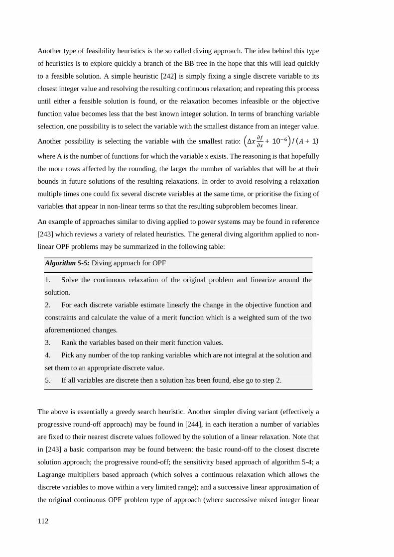
112
Another type of feasibility heuristics is the so called diving approach. The idea behind this type
of heuristics is to explore quickly a branch of the BB tree in the hope that this will lead quickly
to a feasible solution. A simple heuristic [242] is simply fixing a single discrete variable to its
closest integer value and resolving the resulting continuous relaxation; and repeating this process
until either a feasible solution is found, or the relaxation becomes infeasible or the objective
function value becomes less that the best known integer solution. In terms of branching variable
selection, one possibility is to select the variable with the smallest distance from an integer value.
Another possibility is selecting the variable with the smallest ratio: Δ푥 + 10 /(퐴 + 1)
where A is the number of functions for which the variable x exists. The reasoning is that hopefully
the more rows affected by the rounding, the larger the number of variables that will be at their
bounds in future solutions of the resulting relaxations. In order to avoid resolving a relaxation
multiple times one could fix several discrete variables at the same time, or prioritise the fixing of
variables that appear in non-linear terms so that the resulting subproblem becomes linear.
An example of approaches similar to diving applied to power systems may be found in reference
[243] which reviews a variety of related heuristics. The general diving algorithm applied to non-
linear OPF problems may be summarized in the following table:
Algorithm 5-5: Diving approach for OPF
1. Solve the continuous relaxation of the original problem and linearize around the
solution.
2. For each discrete variable estimate linearly the change in the objective function and
constraints and calculate the value of a merit function which is a weighted sum of the two
aforementioned changes.
3. Rank the variables based on their merit function values.
4. Pick any number of the top ranking variables which are not integral at the solution and
set them to an appropriate discrete value.
5. If all variables are discrete then a solution has been found, else go to step 2.
The above is essentially a greedy search heuristic. Another simpler diving variant (effectively a
progressive round-off approach) may be found in [244], in each iteration a number of variables
are fixed to their nearest discrete values followed by the solution of a linear relaxation. Note that
in [243] a basic comparison may be found between: the basic round-off to the closest discrete
solution approach; the progressive round-off; the sensitivity based approach of algorithm 5-4; a
Lagrange multipliers based approach (which solves a continuous relaxation which allows the
discrete variables to move within a very limited range); and a successive linear approximation of
the original continuous OPF problem type of approach (where successive mixed integer linear
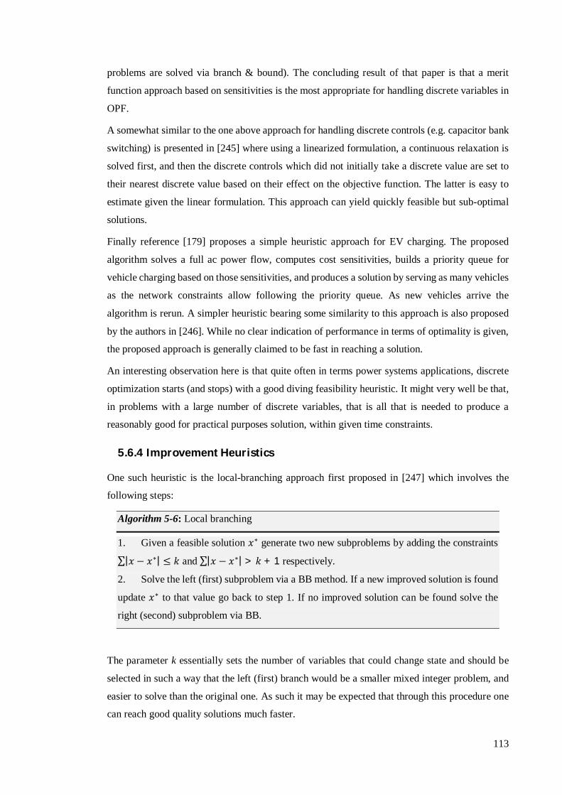
113
problems are solved via branch & bound). The concluding result of that paper is that a merit
function approach based on sensitivities is the most appropriate for handling discrete variables in
OPF.
A somewhat similar to the one above approach for handling discrete controls (e.g. capacitor bank
switching) is presented in [245] where using a linearized formulation, a continuous relaxation is
solved first, and then the discrete controls which did not initially take a discrete value are set to
their nearest discrete value based on their effect on the objective function. The latter is easy to
estimate given the linear formulation. This approach can yield quickly feasible but sub-optimal
solutions.
Finally reference [179] proposes a simple heuristic approach for EV charging. The proposed
algorithm solves a full ac power flow, computes cost sensitivities, builds a priority queue for
vehicle charging based on those sensitivities, and produces a solution by serving as many vehicles
as the network constraints allow following the priority queue. As new vehicles arrive the
algorithm is rerun. A simpler heuristic bearing some similarity to this approach is also proposed
by the authors in [246]. While no clear indication of performance in terms of optimality is given,
the proposed approach is generally claimed to be fast in reaching a solution.
An interesting observation here is that quite often in terms power systems applications, discrete
optimization starts (and stops) with a good diving feasibility heuristic. It might very well be that,
in problems with a large number of discrete variables, that is all that is needed to produce a
reasonably good for practical purposes solution, within given time constraints.
5.6.4 Improvement Heuristics
One such heuristic is the local-branching approach first proposed in [247] which involves the
following steps:
Algorithm 5-6: Local branching
1. Given a feasible solution 푥∗ generate two new subproblems by adding the constraints
∑|푥 − 푥∗| ≤ 푘 and ∑|푥 − 푥∗| > 푘 + 1 respectively.
2. Solve the left (first) subproblem via a BB method. If a new improved solution is found
update 푥∗ to that value go back to step 1. If no improved solution can be found solve the
right (second) subproblem via BB.
The parameter k essentially sets the number of variables that could change state and should be
selected in such a way that the left (first) branch would be a smaller mixed integer problem, and
easier to solve than the original one. As such it may be expected that through this procedure one
can reach good quality solutions much faster.
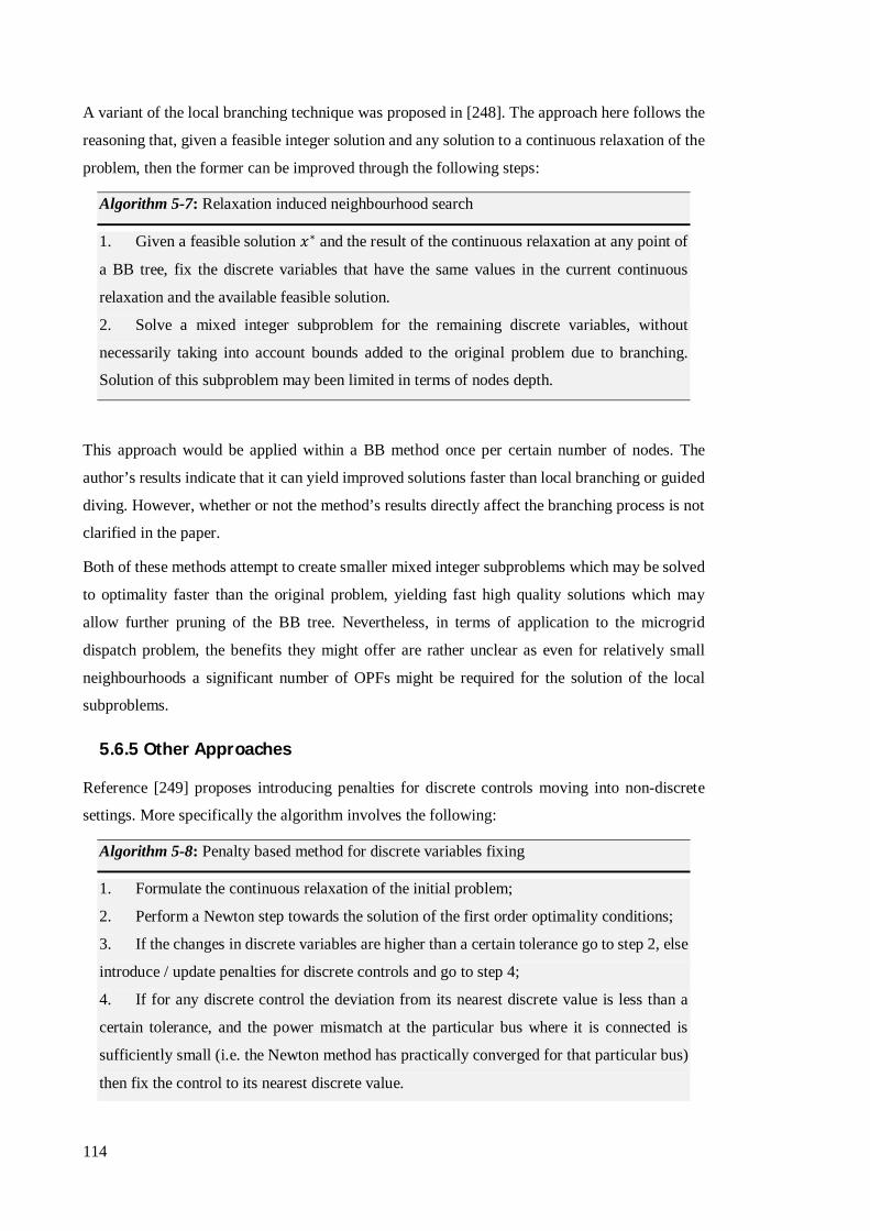
114
A variant of the local branching technique was proposed in [248]. The approach here follows the
reasoning that, given a feasible integer solution and any solution to a continuous relaxation of the
problem, then the former can be improved through the following steps:
Algorithm 5-7: Relaxation induced neighbourhood search
1. Given a feasible solution 푥∗ and the result of the continuous relaxation at any point of
a BB tree, fix the discrete variables that have the same values in the current continuous
relaxation and the available feasible solution.
2. Solve a mixed integer subproblem for the remaining discrete variables, without
necessarily taking into account bounds added to the original problem due to branching.
Solution of this subproblem may been limited in terms of nodes depth.
This approach would be applied within a BB method once per certain number of nodes. The
author’s results indicate that it can yield improved solutions faster than local branching or guided
diving. However, whether or not the method’s results directly affect the branching process is not
clarified in the paper.
Both of these methods attempt to create smaller mixed integer subproblems which may be solved
to optimality faster than the original problem, yielding fast high quality solutions which may
allow further pruning of the BB tree. Nevertheless, in terms of application to the microgrid
dispatch problem, the benefits they might offer are rather unclear as even for relatively small
neighbourhoods a significant number of OPFs might be required for the solution of the local
subproblems.
5.6.5 Other Approaches
Reference [249] proposes introducing penalties for discrete controls moving into non-discrete
settings. More specifically the algorithm involves the following:
Algorithm 5-8: Penalty based method for discrete variables fixing
1. Formulate the continuous relaxation of the initial problem;
2. Perform a Newton step towards the solution of the first order optimality conditions;
3. If the changes in discrete variables are higher than a certain tolerance go to step 2, else
introduce / update penalties for discrete controls and go to step 4;
4. If for any discrete control the deviation from its nearest discrete value is less than a
certain tolerance, and the power mismatch at the particular bus where it is connected is
sufficiently small (i.e. the Newton method has practically converged for that particular bus)
then fix the control to its nearest discrete value.
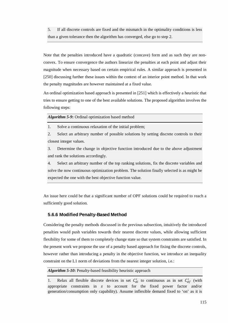
115
5. If all discrete controls are fixed and the mismatch in the optimality conditions is less
than a given tolerance then the algorithm has converged, else go to step 2.
Note that the penalties introduced have a quadratic (concave) form and as such they are non-
convex. To ensure convergence the authors linearize the penalties at each point and adjust their
magnitude when necessary based on certain empirical rules. A similar approach is presented in
[250] discussing further these issues within the context of an interior point method. In that work
the penalty magnitudes are however maintained at a fixed value.
An ordinal optimization based approach is presented in [251] which is effectively a heuristic that
tries to ensure getting to one of the best available solutions. The proposed algorithm involves the
following steps:
Algorithm 5-9: Ordinal optimization based method
1. Solve a continuous relaxation of the initial problem;
2. Select an arbitrary number of possible solutions by setting discrete controls to their
closest integer values.
3. Determine the change in objective function introduced due to the above adjustment
and rank the solutions accordingly.
4. Select an arbitrary number of the top ranking solutions, fix the discrete variables and
solve the now continuous optimization problem. The solution finally selected is as might be
expected the one with the best objective function value.
An issue here could be that a significant number of OPF solutions could be required to reach a
sufficiently good solution.
5.6.6 Modified Penalty-Based Method
Considering the penalty methods discussed in the previous subsection, intuitively the introduced
penalties would push variables towards their nearest discrete values, while allowing sufficient
flexibility for some of them to completely change state so that system constraints are satisfied. In
the present work we propose the use of a penalty based approach for fixing the discrete controls,
however rather than introducing a penalty in the objective function, we introduce an inequality
constraint on the L1 norm of deviations from the nearest integer solution, i.e.:
Algorithm 5-10: Penalty-based feasibility heuristic approach
1. Relax all flexible discrete devices in set 퐶∗ to continuous as in set 퐶∗ (with appropriate constraints in 푠 to account for the fixed power factor and/or generation/consumption only capability). Assume inflexible demand fixed to ‘on’ as it is

116
reasonable to assume that the network is designed to serve it. Solve the resulting approximate OPF using O2. If there are voltage violations, then also relax inflexible demand and repeat the solution. 2. Let 푥∗ denote the solution of this problem with respect to the discrete variables, 푥∗ the nearest integer solution and let Δ푥 = |푥∗ − 푥∗|. Resolve the relaxed problem using algorithm O2 with the additional constraint |푥 − 푥∗| ≤ 휌Δ푥, where 0 < 휌 ≤ 1. 3. Update 푥∗, Δ푥. If Δ푥 ≤ 휀 then a feasible solution has been found, else go back to 1.
The reasoning behind our approach is that a penalty in the objective function would either be too
small (as such it would have little impact on the outcome) or significantly large (as such it would
directly force the solution to the nearest integer). On the contrary the inequality constraint should
force the variables to which the solution is less sensitive to, to their nearest discrete values, while
allowing for the remaining to change state so that there is no significant deviation in terms of
objective function value. The parameter 휌 may be used to adjust the expected convergence speed
(i.e. a lower value would imply less iterations but possibly less optimal solution).
Our test cases involve modified versions of IEEE test feeders, where we have introduced at each
node one EV per 6kW of demand (assuming this is the average household consumption), set 푃
at 1.5 times the original feeder demand (i.e. not all EVs can be covered at the current time step)
and 휌 = 0.4. The following table summarizes the test results:
Table 5-2: Performance of algorithm 5-10 Tap controls
number Added EVs
number Solution
time (sec) IEEE-13 3 592 7.7 IEEE-34 9 316 4.3 IEEE-37 3 409 4.9 IEEE-123 9 623 14.9
The cases studied were characterized by a large number of discrete controls of small individual
size. As such the discrete solution was generally close to the initial continuous relaxation. Of
course for problems where a limited number of large controls is also available, then the proposed
method could be used as a local search in a branch and bound algorithm at the nodes of which the
large controls are fixed to discrete values. Typically, given that this problem is assumed to be
solved every few minutes, a good initial point would generally be available. With this taken into
account the presented solution times could be significantly shorter.
5.7 Conclusions & Further Questions
The overall changes in our framework our summarized in Fig.5-2, and effectively relate to the
centralized solution approach of the microgrid problem. It should be noted that in terms of integer
device controls our approach is essentially a heuristic and cannot guarantee the actual optimum.

117
Nevertheless, most current literature appears to indicate that for real-time applications a full
branch & bound solution might be untenable. Especially if a large number of discrete device
controls is involved. Furthermore, given the uncertainty that is prevalent in distribution (i.e.
network parameters, exact power drawn from individual devices) an exact optimal solution in
terms of losses might be of little practical interest. Losses at distribution may be a problem of
infrastructure rather than energy management. As such, a reliable heuristic that guarantees a
‘good’ feasible solution in whatever time is available might be all that is needed here. After all,
that is also a fundamental component of any branch & bound method that looks for the actual
optimum.
Fig.5-2: Conceptual energy management framework. The arrows represent transmission of information. This framework and presented solution approach may be extended to take particular market rules and penalties into account.

119
6 Conclusions
The work presented in the previous subsections constitutes a first step towards building an energy management framework for future energy networks with significant flexible resources penetration and an extensive integrated telecommunications infrastructure. But there are several more questions that need to be answered. The following paragraphs provide an overview of the presented work and identify what needs to be done next.
6.1 A Brief Summary
The major contribution of this work is the development of a novel general framework that
addresses the two basic shortcomings of today’s energy management mechanisms: 1) managing
flexible devices (such as EVs, etc.) located at any level in the power system and coordinating
them over time; 2) optimizing energy management in the system subject to distribution network
constraints. An important and perhaps most distinctive characteristic of our approach is that each
ensuing optimization problem is clearly associated with a specific scope and time-frame of
application. The proposed framework consists of two basic close to real-time mechanisms /
optimization problems: an extended Economic Dispatch and a newly formulated Microgrid
Dispatch. Within each of these mechanisms, through the proposed formulations and solution
approaches, several smaller research contributions arise from the present work. More specifically,
within the context of ED:
(Chapter 3) One fully parallelizable distributed optimization technique (ADMM) has been applied to the solution of the optimal power flow, which to our knowledge had not been used before in the full ac problem. (Chapter 3) The ADMM method is one of the most promising distributed optimization
techniques for decentralized solution purposes and quite representative of a larger class of relevant methods. The investigation carried out with regards to the extent to which decentralization can be pushed, both in terms of network decomposition and user disaggregation provides insight into how these methods work and how they could be used. (Chapter 3) Different decomposition structures for the centralized problem were investigated
and a two-level decomposition scheme was proposed for decentralized operations in the power system. This would allow combining different optimization techniques based on the characteristics of each subproblem, and could significantly improve convergence. (Chapter 4) A new multi-period formulation for the economic dispatch problem was proposed
based on the uncertainty associated with each node (or sets of nodes) in the system. Within this context we redefined the concept of the microgrid as a collection of devices / part of the network for which a reasonably accurate power injection forecast is feasible.
120
Furthermore, with respect to the MD mechanism:
(Chapter 2) We propose a novel formulation and solution approach for optimal power flow problems on unbalanced ac networks. This approach is based on the observation that voltage angles in such networks are typically small, and uses a number of appropriate voltage reference frame transformations to ensure accurate results. (Chapter 5) We build a trust-region based approach to further optimize tap changing positions.
This iterative approach solves a series of convex, largely linearly constrained, subproblems compared to the non-linear original problem. (Chapter 5) We propose a simple penalty based approach for determining discrete controls
settings. This approach is efficient when dealing with problems where a large number of small discrete controls are available, and as such the optimal integral solution may be expected to be quite close to that of the continuous relaxation.
Overall our framework may also be summarized in the algorithmic flowcharts of Fig.6-1. As may
be seen apart from the general contributions mentioned above several other issues were involved
and investigated, namely: the formulation of balanced ac network constraints; representation of
unbalanced ac network constraints and relevant power quality requirements; mathematical
methods for the centralized solution of optimal power flow problems; and mathematical methods
for integer problems. In their full detail these are all subjects with much research potential.
As it stands our framework puts the application of decentralized methods in power systems into
perspective, and provides a basic reference formulation and solution to the optimization problems
associated with close to real-time energy management. The presented results throughout this work
appear promising in terms of a possible practical application of such an approach. However, as
we discuss in the following, several more steps need to be taken towards that goal.
6.2 Further Improvements & Extensions
The flowcharts of Fig.6-1 illustrate the problems solved as part of this work, but also indicate
improvements that could be made. Following is a list of the latter along with a brief explanation:
Modelling aggregate microgrid flexibility (1): The model we presented in Chapter 4 is one
practical approach for modelling this flexibility when considering mainly renewables and
unidirectional EVs. But an extension would be required to take into account any smart household
appliances, storage, or any other flexible devices.
Network partitioning for optimization (2): In this work we used a spectral partitioning
approach in order to split the network, but it may be that for the purpose of distributed
computations more efficient approaches are available. This however might be a question of
mostly academic interest.
Contingency constraints (2): Practical transmission-level optimisation problems typically
include an additional set of constraints which ensure safe system operation in case of a component
outage. This presupposes identifying a subset of important (problematic) contingencies and

121
extending the OPF formulation to account for the actions that need to be taken if these occur. This
would lead to an even larger transmission network subproblems which would need to be
efficiently solved, but also make any attempt at network decomposition much harder.
Constraint management (3), (4), (5), (6): Given that decentralized approaches are iterative
techniques, introducing a more efficient management of active constraints within these
subproblems could greatly improve computational efficiency.
Auxiliary services (reserves) (3), (4), (5), (6): Apart from reactive power, another quantity
that is of interest in OPF problems is reserves, i.e. how much power a device could additionally
supply (or withdraw) from the network in case that is urgently needed (either due to demand /
renewables variations or certain faults). This is one additional parameter that could be
incorporated into the decentralized framework.
Communications reliability & delays (7), (9): This is an important question that has not been
considered in detail. As it should be clear from the preceding chapters, communications latency
Fig.6-1: Algorithmic flowcharts summarizing the parts involved in our proposed energy management framework (top) and the interior point method developed and used for the solution of the vast majority of optimization subproblems in this work (bottom). The numbers indicate smaller individual problems.

122
can have a big impact in the viability of any decentralized scheme. Modelling more accurately
the associated delays and evaluating their impact is a subject of particular interest.
Managing microgrid uncertainty (1), (11): Uncertainty in our scheme is managed in two
steps: when building the aggregate flexibility model, and when formulating the microgrid
dispatch problem. However, one aspect that has not been fully explored in this work is how these
two different formulations interact.
Improving the trust-region mechanism (13), (14), (16): Within this work we use the interior
point method for most individual subproblems. However, it may be that other algorithms could
perform better in these types of problems, e.g. by taking better advantage of a warm-start. In
addition, instead of solving a second exact subproblem for evaluation of the tap updates, there
might be an approximate calculation that could be used to speed up solution times.
Solving for discrete controls (17): The simple penalty approach proposed here will work
effectively with problems where a variety of smaller discrete controls contribute to the solution,
as in the cases tested. However, if a number of high impact controls were available then this
approach might not necessarily produce the best possible solution and alternative methods might
have to be investigated. However relevant testing requires adequately good real-world test cases.
Improving the interior-point solver: While this general purpose solver works adequately well,
how it could be improved is an important consideration. Given the vast number of individual
subproblems that have to be solved even a small improvement here, could mean a significant
improvement for the overall scheme convergence time.
These summarize several considerations which could help towards getting the proposed
framework closer to practical application. Of course the hardware part for its implementation is
an open question by itself. Once all possible improvements on the power systems side have been
made, the scope of the present work may be directly extended beyond power systems in their
classical form, i.e. towards larger scale optimization problems integrating also other types of
energy systems.

123
7 References
[1] Z. Zhu, Optimization of Power System Operation, IEEE - Wiley, 2009.
[2] P. Kundur, Power System Stability and Control, McGraw-Hill, 1994.
[3] Q. P. Zheng, J. Wang and A. L. Liu, “Stochastic Optimization for Unit Commitment - A Review,” IEEE Trans. Power Systems, vol. 30, no. 4, pp. 1913-1924, 2015.
[4] GE Energy, “Review of Industry Practice and Experience in the Integration of Wind and Solar Generation,” November 2012. [Online]. Available: http://www.pjm.com.
[5] M. B. Cain, R. P. O'Neill and A. Castillo, “History of Optimal Power Flow and Formulations,” 2012. [Online]. Available: http://www.ferc.gov/.
[6] S. Stoft, Power System Economics, IEEE Press & Wiley-Interscience, 2002.
[7] M. Shahidehpour, H. Yamin and Z. Li, Market Operations in Electric Power Systems, IEEE Press & Wiley-Interscience, 2002.
[8] R. Leou, C. Su and C. Lu, “Stochastic analyses of electric vehicle charging impacts on distribution network,” IEEE Trans. Power Systems, vol. 29, no. 3, pp. 1055-1063, 2014.
[9] S. Nykamp, M. D. C. Bosman, A. Molderink, J. L. Hurink and G. J. M. Smit, “Value of storage in distribution grids - Competition or cooperation of stakeholders,” IEEE Trans. Smart Grid, vol. 4, no. 3, pp. 1361-1370, 2013.
[10] M. Pipattanasomporn, M. Kuzlu, S. Rahman and Y. Teklu, “Load Profiles of Selected Major Household Appliances and Their Demand Response Opportunities,” IEEE Trans. Smart Grid, vol. 5, no. 2, pp. 742-750, 2014.
[11] L. P. Fernandez, T. G. S. Roman, R. Cossent, C. M. Domingo and P. Frias, “Assessment of the Impact of Plug-in Electric Vehicles on Distribution Networks,” IEEE Trans. Power Systems, vol. 26, no. 1, pp. 206-213, 2011.
[12] P. Zhang, K. Qian, C. Zhou, B. G. Stewart and D. M. Hepburn, “A Methodology for Optimization of Power Systems Demand Due to Electric Vehicle Charging Load,” IEEE Trans. Power Systems, vol. 27, no. 3, pp. 1628-1636, 2012.
[13] D. P. Bertsekas and J. N. Tsitsiklis, Parallel and Distributed Computation: Numerical Methods, Athena Scientific, 1997.
[14] M. G. Vaya and G. Andersson, “Optimal Bidding Strategy of a Plug-In Electric Vehicle Aggregator in Day-Ahead Electricity Markets Under Uncertainty,” IEEE Trans. Power Systems, vol. 30, no. 5, pp. 2375-2385, 2015.
[15] S. Vandael, B. Claessens, M. Hommelberg, T. Holvoet and G. Deconinck, “A Scalable Three-Step Approach for Demand Side Management of Plug-in Hybrid Vehicles,” IEEE Trans. Smart Grid, vol. 4, no. 2, pp. 720-728, 2013.

124
[16] N. Rotering and M. Ilic, “Optimal Charge Control of Plug-In Hybrid Electric Vehicles in Deregulated Electricity Markets,” IEEE Trans. Power Systems, vol. 26, no. 3, pp. 1021-1029, 2011.
[17] R. J. Bessa, M. A. Matos, F. J. Soares and J. A. P. Lopes, “Optimized Bidding of a EV Aggregation Agent in the Electricity Market,” IEEE Trans. Smart Grid, vol. 3, no. 1, pp. 443-452, 2012.
[18] M. Pantos, “Exploitation of Electric-Drive Vehicles in Electricity Markets,” IEEE Trans. Power Systems, vol. 27, no. 2, pp. 682-694, 2012.
[19] S. I. Vagropoulos and A. G. Bakirtzis, “Optimal Bidding Strategy for Electric Vehicle Aggregators in Electricity Markets,” IEEE Trans. Power Systems, vol. 28, no. 4, pp. 4031-4041, 2014.
[20] J. M. Foster and M. C. Caramanis, “Optimal Power Market Participation of Plug-In Electric Vehicles Pooled by Distribution Feeder,” IEEE Trans. Power Systems, vol. 28, no. 3, pp. 2065-2076, 2013.
[21] C. Jin, J. Tang and P. Ghosh, “Optimizing Electric Vehicle Charging With Energy Storage in the Electricity Market,” IEEE Trans. Smart Grid, vol. 28, no. 3, pp. 2065-2076, 2013.
[22] Y. Dvorkin, H. Pandzic, M. A. Ortega-Vazquez and D. S. Kirschen, “A Hybrid Stochastic/Interval Approach to Transmission-Constrained Unit Commitment,” IEEE Trans. Power Systems, vol. 30, no. 2, pp. 621-631, 2015.
[23] M. A. Ortega-Vazquez, F. Bouffard and V. Silva, “Electric Vehicle Aggregator/System Operator Coordination for Charging Scheduling and Services Procurement,” IEEE Trans. Power Systems, vol. 28, no. 2, pp. 1806-1815, 2013.
[24] E. A. Bakirtzis, P. N. Biskas, D. P. Labridis and A. G. Bakirtzis, “Multiple Time Resolution Unit Commitment for Short-Term Operations Scheduling Under High Renewable Penetration,” IEEE Trans. Power Systems, vol. 29, no. 1, pp. 149-159, 2014.
[25] A. T. Al-Alwami and E. Sortomme, “Coordinating Vehicle-to-Grid Services With Energy Trading,” IEEE Trans. Smart Grid, vol. 3, no. 1, pp. 453-458, 2012.
[26] H. Heitsch and W. Romisch, “Scenario redution algorithms in stochastic programming,” Comput. Optim. Appl., vol. 24, no. 2, pp. 187-206, 2003.
[27] O. Alsac and B. Stott, “Optimal Load Flow with Steady-State Security,” IEEE Trans. Power Apparatus and Systems, vol. 93, no. 3, pp. 745-751, 1974.
[28] W. H. Kersting, Distribution System Modeling and Analysis, CRC Press, 2002.
[29] F. Corcoles, L. Sainz, J. Pedra, J. Sanchez-Navarro and M. Salichs, “Three-phase transformer modelling for unbalanced conditions - Part I: core modelling and introductory examples,” IET Electr. Power Appl., vol. 2, no. 2, pp. 99-112, 2008.
[30] F. Corcoles, L. Sainz, J. Pedra, J. Sanchez-Navarro and M. Salichs, “Three-phase transformer modelling for unbalanced conditions - Part II: general formulation,” IET Electric Power Applications, vol. 3, no. 1, pp. 19-39, 2007.
[31] L. R. Araujo, D. R. R. Penido, S. Carneiro and J. L. R. Pereira, “A Three-Phase Optimal Power-Flow Algorithm to Mitigate Voltage Unbalance,” IEEE Trans. Power Delivery, vol. 28, no. 4, pp. 2394-2402, 2013.
[32] T. Cutsem and C. Vournas, Voltage Stability of Electric Power Systems, Kluwer Academic Publishers, 1998.
[33] A. Bokhari, A. Alkan, R. Dogan, M. Diaz-Aguilo, F. Leon, D. Czarkowski, Z. Zabar, L. Birenbaum, A. Noel and R. E. Uosef, “Experimental Determination of the ZIP Coefficients for Modern

125
Residential, Commercial, and Industrial Loads,” IEEE Trans. Power Delivery, vol. 29, no. 3, pp. 1372-1381, 2014.
[34] D. Kirschen and G. Strbak, Fundamentals of Power Systems Economics, Wiley, 2004.
[35] M. E. Baran and F. F. Wu, “Optimal Capacitor Placement on Radial Distribution Systems,” IEEE Trans. Power Delivery, vol. 4, no. 1, pp. 725-734, 1989.
[36] H. D. Chiang and M. E. Baran, “On the Existence and Uniqueness of Load Flow Solution for Radial Distribution Power Networks,” IEEE Trans. Circuits and Systems, vol. 37, no. 3, pp. 410-416, 1990.
[37] R. G. Cespedes, “New Method for the Analysis of Distribution Networks,” IEEE Trans. Power Delivery, vol. 5, no. 1, pp. 391-396, 1990.
[38] M. Farivar and S. H. Low, “Branch Flow Model: Relaxations and Convexification - Part I,” IEEE Trans. Power Systems, vol. 28, no. 3, pp. 2554-2564, 2013.
[39] Y.-C. Chang, W.-T. Yang and C.-C. Liu, “A New Method for Calculating Loss Coefficients,” IEEE Trans. Power Systems, vol. 9, no. 3, pp. 1665-1671, Aug. 1994.
[40] A. K. Kazerooni and J. Mutale, “Transmission Network Planning Under Security and Environmental Constraints,” IEEE Trans. Power Systems, vol. 25, no. 2, pp. 1169-1178, May 2010.
[41] F. Li and R. Bo, “DCOPF-Based LMP Simulation: Algorithm, Comparison with ACOPF, and Sensitivity,” IEEE Trans. Power Systems, vol. 22, no. 4, pp. 1475-1485, 2007.
[42] X. Bai, H. Wei, K. Fujisawa and Y. Wang, “Semidefinite Programming for Optimal Power Flow Problems,” Electrical Power and Energy Systems, vol. 30, no. 6-7, pp. 383-392, 2008.
[43] J. Lavaei and S. H. Low, “Convexification of Optimal Power Flow Problem,” in 48th Allerton Conference on Communications, Control & Computing, Allerton, USA, 2010.
[44] J. Lavaei and S. H. Low, “Zero Duality Gap in Optimal Power Flow Problem,” IEEE Trans. on Power Systems, vol. 27, no. 1, pp. 92-107, 2012.
[45] J. Lavaei, “Zero Duality Gap for Classical OPF Problem Convexifies Fundamental Nonlinear Power Problems,” in American Control Conference, San Francisco, USA, 2011.
[46] S. Bose, D. F. Gayme, S. Low and K. M. Chandy, “Optimal Power Flow Over Tree Networks,” in 49th Annual Allerton Conference on Communication, Control & Computing, Monticello, USA, 2011.
[47] B. C. Lesieutre, D. K. Molzahn, A. R. Borden and C. L. DeMarco, “Examining the Limits of the Application fo Semidefinite Programming to Power Flow Problems,” in 49th Annual Allerton Conference on Communication, Control & Computing, Monticello, USA, 2011.
[48] J. Lavaei, D. Tse and B. Zhang, “Geometry of Power Flows and Optimization in Distribution Networks,” IEEE Trans. Power Systems, vol. 29, no. 2, pp. 572-583, 2014.
[49] R. Madani, S. Sojoudi and J. Lavaei, “Convex Relaxation for Optimal Power Flow Problem: Mesh Networks,” IEEE Trans. Power Systems, vol. 30, no. 1, pp. 199-211, 2015.
[50] M. Farivar and S. H. Low, “Branch Flow Model: Relaxations and Convexification - Part II,” IEEE Trans. Power Systems, vol. 28, no. 3, pp. 2565-2572, 2013.
[51] B. Subhonmesh, S. H. Low and K. M. Chandy, “Equivalence of Branch Flow and Bus Injection Models,” in 50th Annual Allerton Conference on Communication, Control & Computing, Monticello, USA, 2012.
[52] N. Li, L. Chen and S. Low, “Exact Convex Relaxation for Radial Networks Using Branch Flow Models,” in IEEE International Conference in Smart Grid Communications, Tainan, Taiwan, 2012.
126
[53] R. A. Jabr, “Radial Distribution Load Flow Using Conic Programming,” IEEE Trans. Power Systems, vol. 21, no. 3, pp. 1458-1459, 2006.
[54] R. A. Jabr, “Optimal Power Flow Using an Extended Conic Quadratic Formulation,” IEEE Trans. Power Systems, vol. 23, no. 3, pp. 1000-1008, 2008.
[55] J. A. Taylor, Convex optimisation of power systems, Cambridge University Press, 2015.
[56] C. S. Cheng and D. Shirmohammadi, “A Three-Phase Power Flow Method for Real-Time Distribution System Analysis,” IEEE Trans. Power Systems, vol. 10, no. 2, pp. 671-679, 1995.
[57] M. Abdel-Akher, K. M. Nor and A. H. A. Rashid, “Improved Three-Phase Power-Flow Methods Using Sequence Components,” IEEE Trans. Power Systems, vol. 20, no. 3, pp. 1389-1397, 2005.
[58] Y. Cao, Y. Tan, C. Li and C. Rehtanz, “Chance-Constrained Optimization-Based Unbalanced Optimal Power Flow for Radial Distribution Networks,” IEEE Trans. Power Delivery, vol. 28, no. 3, pp. 1855-1864, 2013.
[59] M. Z. Kamh and R. Iravani, “Unbalanced Model and Power-Flow Analysis of Microgrids and Active Distribution Systems,” IEEE Trans. Power Delivery, vol. 25, no. 4, pp. 2851-2858, 2010.
[60] D. R. R. Penido, L. R. Araujo, S. Carneiro, J. L. R. Pereira and P. A. N. Garcia, “Three-phase Power Flow Based on Four-Conductor Current Injection Method for Unbalanced Distribution Networks,” IEEE Trans. Power Systems, vol. 23, no. 2, pp. 494-503, 2008.
[61] P. A. N. Garcia, J. L. R. Pereira, S. Carneiro, V. M. Costa and N. Martins, “Three-phase power flow calculations using the current injection method,” IEEE Trans. Power Systems, vol. 15, no. 2, pp. 508-514, 2000.
[62] R. M. Ciric, A. P. Feltrin and L. F. Ochoa, “Power Flow in Four-Wire Distribution Networks - General Approach,” IEEE Trans. Power Systems, vol. 18, no. 4, pp. 1283-1290, 2003.
[63] A. O'Connell, D. Flynn and A. Keane, “Rolling Multi-Period Optimization to Control Electric Vehicle Charging in Distribution Networks,” IEEE Trans. Power Systems, vol. 29, no. 1, pp. 340-348, 2014.
[64] CENELEC Std. EN-50160, “Voltage characteristics of electricity supplied by public electricity networks,” 2010.
[65] P. Pillay and M. Manyage, “Definitions of Voltage Unbalance,” IEEE Power Engineering Review, vol. 21, no. 5, pp. 49-51, 2001.
[66] M. H. J. Bollen, “Definitions of Voltage Unbalance,” IEEE Power Engineering Review, vol. 22, no. 11, pp. 49-50, 2002.
[67] J. R. Marti, H. Ahmadi and L. Bashualdo, “Linear Power-Flow Formulation Based on a Voltage-Dependent Load Model,” IEEE Trans. Power Delivery, vol. 28, no. 3, pp. 1682-1690, 2013.
[68] R. S. Ferreira, C. L. T. Borges and M. V. F. Pereira, “A Flexible Mixed-Integer Linear Programming Approach to the AC Optimal Power Flow in Distribution,” IEEE Trans. Power Systems, vol. 29, no. 5, pp. 2447-2459, 2014.
[69] W. H. Kersting, “Radial distribution test feeders,” IEEE Trans. Power Systems, vol. 6, no. 3, pp. 975-985, 1991.
[70] “Distribution Test Feeders,” [Online]. Available: http://ewh.ieee.org/soc/pes/dsacom/testfeeders/index.html.
[71] J. Nocedal and S. J. Wright, Numerical Optimization, Springer, 2006.
127
[72] S. Bruno, S. Lamonaca, G. Rotondo, U. Stecchi and M. LaScala, “Unbalanced Three-Phase Optimal Power Flow for Smart Grids,” IEEE Trans. Industrial Electronics, vol. 58, no. 10, pp. 4504-4513, 2011.
[73] F. Palacios-Gomez, L. Lasdon and M. Engquist, “Nonlinear optimization by successive linear programming,” Management Science, vol. 28, no. 10, pp. 1106-1120, 1982.
[74] B. Stott and J. L. Marinho, “Linear Programming for Power System Network Security Applications,” IEEE Trans. Power Apparatus & Systems, vol. 98, no. 3, pp. 837-848, 1979.
[75] O. Alsac, J. Bright, M. Prais and B. Stott, “Further Developments in LP-Based Optimal Power Flow,” IEEE Trans. Power Systems, vol. 5, no. 3, pp. 697-711, 1990.
[76] C. Campaigne, P. A. Lipka, M. Pirnia, R. P. O'Neill and S. Oren, “Testing Step-Size Limits for Solving the Linearized Current Voltage AC Optimal Power Flow,” 2013. [Online]. Available: http://www.ferc.gov/.
[77] I. M. Nejdawi, K. A. Clements and P. W. Davis, “An Efficient Interior Point Methods for Sequential Quadratic Programming Optimal Power Flow,” IEEE Trans. Power Systems, vol. 15, no. 4, pp. 1179-1183, 2000.
[78] S. Boyd and L. Vandenberghe, Convex Optimization, Cambridge University Press, 2004.
[79] R. J. Vanderbei and D. F. Shanno, “An interior-point algorithm for nonconvex nonlinear programming,” Computational Optimization and Applications, vol. 13, no. 1, pp. 231-252, 1999.
[80] R. D. Zimmerman, C. E. Murillo-Sanchez and R. J. Thomas, “MATPOWER: Steady-state operations, planning, and analysis tools for power systems research and education,” IEEE Trans. Power Systems, vol. 26, no. 1, pp. 12-19, 2011.
[81] H. Wang, C. E. Murillo-Sanchez, R. D. Zimmerman and R. J. Thomas, “On Computational Issues of Market-Based Optimal Power Flow,” IEEE Trans. Power Systems, vol. 22, no. 3, pp. 1185-1193, 2007.
[82] V. H. Quintana, G. L. Torres and J. Medina-Palomo, “Interior-point methods and their applications to power systems: A classification of publications and software codes,” IEEE Trans. Power Systems, vol. 15, no. 1, pp. 170-176, 2000.
[83] S. Granville, “Optimal reactive dispatch through interior point methods,” IEEE Trans. Power Systems, vol. 9, no. 1, pp. 136-146, 1994.
[84] X. Yan and H. Quintana, “An infeasible interior-point algorithm for optimal power-flow problems,” Electric Power Systems Research, vol. 39, no. 1, pp. 39-46, 1996.
[85] C. N. Lu and M. R. Unum, “Network constrained security control using an interior point algorithm,” IEEE Trans. Power Systems, vol. 8, no. 3, pp. 1068-1076, 1993.
[86] X. Yan and V. H. Quintana, “Improving an Interior-Point-Based OPF by dynamic adjustments of step sizes and tolerances,” IEEE Trans. Power Systems, vol. 14, no. 2, pp. 709-717, 1999.
[87] Y. Wu, A. S. Debs and R. E. Marsten, “A direct nonlinear Predictor-Corrector Primal-Dual Interior Point algorithm for optimal power flows,” IEEE Trans. Power Systems, vol. 9, no. 2, pp. 876-883, 1994.
[88] F. Capitanescu, M. Glavic, D. Ernst and L. Wehenkel, “Interior-point based algorithms for the solution of optimal power flow problems,” Electric Power Systems Research, vol. 77, no. 5, pp. 508-517, 2007.
128
[89] G. D. Irisarri, X. Wang, J. Tong and S. Mokhtari, “Maximum loadability of power systems using interior point non-linear optimization method,” IEEE Trans. Power Systems, vol. 12, no. 1, pp. 162-172, 1997.
[90] G. L. Torres and V. H. Quintana, “An interior-point method for nonlinear optimal power flow using voltage rectangular coordinates,” IEEE Trans. Power Systems, vol. 13, no. 4, pp. 1211-1218, 1998.
[91] M. J. Rider, C. A. Castro, M. F. Bedrinana and A. V. Garcia, “Towards a fast and robust interior point method for power system applications,” IEE Proc. Gener. Transm. Distrib., vol. 151, no. 5, pp. 575-581, 2004.
[92] G. Tognola and R. Bacher, “Unlimited point algorithm for OPF problems,” IEEE Trans. Power Systems, vol. 14, no. 3, pp. 1046-1054, 1999.
[93] Y. Yuan, “Recent advances in trust region algorithms,” Mathematical Programming, vol. 151, no. 1, pp. 249-281, 2015.
[94] A. A. Sousa, G. L. Torres and C. A. Canizares, “Robust Optimal Power Flow Solution Using Trust Region and Interior-Point Methods,” IEEE Trans. Power Systems, vol. 26, no. 2, pp. 487-499, 2011.
[95] A. Castillo and R. P. O'Neill, “Survey of Approaches to Solving the ACOPF,” 2013. [Online]. Available: http://www.ferc.gov.
[96] C. Guille and G. Gross, “A Conceptual Framework for the Vehicle-to-Grid Implementation,” Energy Policy, vol. 37, no. 11, pp. 4379-4390, 2009.
[97] J. A. P. Lopes, F. J. Soares and P. M. R. Almeida, “Integration of Electric Vehicles in the Electric Power System,” IEEE Proceedings, vol. 99, no. 1, pp. 168-183, 2011.
[98] V. Alimisis and P. C. Taylor, “Zoning Evaluation for Improved Coordinated Automatic Voltage Control,” IEEE Trans. Power Systems, vol. 30, no. 5, pp. 2736-2746, 2015.
[99] A. Y. Ng, M. I. Jordan and Y. Weiss, “On Spectral Clustering: Analysis and an Algorithm,” in Neural Information Processing Systems (NIPS), Vancouver, Canada, 2001.
[100] R. S. Garcia, M. Fennelly, S. Norris, N. Wright, G. Niblo, J. Brodzki and J. Bialek, “Hierarchical Spectral Clustering of Power Grids,” IEEE Trans. Power Systems, vol. 29, no. 5, pp. 2229-2237, 2014.
[101] G. Gan, C. Ma and J. Wu, Data Clustering: Theory, Algorithms and Applications, SIAM, 2007.
[102] A. J. Conejo, E. Castillo, R. Minguez and R. Garcia-Bertrand, Decomposition Techniques in Mathematical Programming: Engineering and Science Applications, Springer, 2006.
[103] J. C. Lopez, M. Granada and J. R. S. Mantovani, “Multi area Decentralized Optimal VAr Planning Using the Dantzig-Wolfe Decomposition Principle,” in IEEE Transmission and Distribution Conference and Exposition (T&D-LA), Sao Paulo, Brazil, 2010.
[104] N. Deeb and S. M. Shahidehpour, “Linear Reactive Power Optimization in a Large Power Network Using the Decomposition Approach,” IEEE Trans. Power Systems, vol. 5, no. 2, pp. 428-438, 1990.
[105] M. Aganagic and S. Mokhtari, “Security Constrained Economic Dispatch Using Nonlinear Dantzig-Wolfe Decomposition,” IEEE Trans. Power Systems, vol. 12, no. 1, pp. 105-112, 1997.
[106] S. Cvijic and J. Xiong, “Security Constrained Unit Commitment and Economic Dispatch Through Benders Decomposition: A Comparative Study,” in IEEE Power and Energy Society General Meeting, San Diego, USA, 2011.

129
[107] D. Phan and J. Kalagnanam, “Distributed Methods for Solving the Security Constrained Optimal Power Flow Problem,” in IEEE Innovative Smart Grid Technologies (ISGT), Washington, USA, 2012.
[108] C. Lemarechal, “The Omnipresence of Lagrange,” Annals of Operation Research, vol. 153, no. 1, pp. 9-27, 2007.
[109] D. P. Bertsekas, Nonlinear Programming, Athena Scientific, 1999.
[110] S. Dekrajangpetch, G. B. Sheble and A. J. Conejo, “Auction Implementation Problems Using Lagrangian Relaxation,” IEEE Trans. Power Systems, vol. 14, no. 1, pp. 82-88, 1999.
[111] W. Ongsakul and N. Petcharaks, “Unit Commitment by Enhanced Adaptive Lagrangian Relaxation,” IEEE Trans. Power Systems, vol. 19, no. 1, pp. 620-628, 2004.
[112] A. Merlin and P. Sandrin, “A New Method for Unit Commitment at Electricite De France,” IEEE Trans. Power Apparatus & Systems, vol. 102, no. 5, pp. 1218-1225, 1983.
[113] A. G. Bakirtzis, “Joint Energy and Reserve Dispatch in a Competitive Pool Using Lagrangian Relaxation,” IEEE Power Engineering Review, vol. 18, no. 11, pp. 60-62, 1998.
[114] A. J. Conejo and J. A. Aguado, “Multi Area Coordinated Decentralized DC Optimal Power Flow,” IEEE Transactions on Power Systems, vol. 13, no. 4, pp. 1272-1278, Nov. 1998.
[115] N. J. Redondo and A. J. Conejo, “Short-Term Hydro-Thermal Coordination by Lagrangian Relaxation: Solution of the Dual Problem,” IEEE Trans. Power Systems, vol. 14, no. 1, pp. 89-95, 1999.
[116] A. L. Motto, F. D. Galiana, A. J. Conejo and M. Huneault, “On Walrasian Equilibrium for Pool-Based Markets,” IEEE Trans. Power Systems, vol. 17, no. 3, pp. 774-781, 2002.
[117] N. Gatsis and G. B. Giannakis, “Decomposition Algorithms for Market Clearing With Large-Scale Demand Response,” IEEE Trans. Smart Grid, vol. 4, no. 4, pp. 1976-1987, 2013.
[118] D. Papadaskalopoulos and G. Strbac, “Decentralized Participation of Flexible Demand in Electricity Markets - Part I: Market Mechanism,” IEEE Trans. Power Systems, vol. 28, no. 4, pp. 3658-3666, 2013.
[119] D. Papadaskalopoulos, G. Strbac, P. Mancarella, M. Aunedi and V. Stanojevic, “Decentralized Participation of Flexible Demand in Electricity Markets - Part II: Application With Electric Vehicles and Heat Pump Systems,” IEEE Trans. Power Systems, vol. 28, no. 4, pp. 3667-3674, 2013.
[120] D. Papadaskalopoulos and G. Strbac, “Decentralized Participation of Electric Vehicles in Network Constrained Market Operation,” in Innovative Smart Grid Technologies (ISGT), Berlin, Germany, 2012.
[121] F. D. Galiana, A. L. Motto, A. J. Conejo and M. Huneault, “Decentralized Nodal-Price Self-Dispatch and Unit Commitment,” in Next Generation of Electric Power Unit Commitment Models, Kluwer, 2001, pp. 271-292.
[122] J. Batut and A. Renaud, “Daily Generation Scheduling Optimization with Transmission Constraints: A New Class of Algorithms,” Trans. Power Systems, vol. 7, no. 3, pp. 982-989, 1992.
[123] D. P. Bertsekas, Constrained Optimization and Lagrange Multiplier Methods, Athena Scientific, 1996.
[124] J. Eckstein, “Parallel Alternating Direction Multiplier Decomposition of Convex Programs,” Journal of Optimization Theory and Applications, vol. 80, no. 1, pp. 39-62, 1994.

130
[125] S. Boyd, N. Parikh, E. Chu, B. Peleato and J. Eckstein, “Distributed Optimization and Statistical Learning via the Alternating Direction Method of Multipliers,” Foundations and Trends in Machine Learning, vol. 3, no. 1, pp. 1-122, 2010.
[126] M. Fukushima, “Application of the Alternating Direction Method of Multipliers to Separable Convex Programming Problems,” Computational Optimization and Applications, vol. 1, no. 1, pp. 93-111, 1992.
[127] B. H. Kim and R. Baldick, “A Comparison of Distributed Optimal Power Flow Algorithms,” IEEE Trans. Power Systems, vol. 15, no. 2, pp. 599-604, May 2000.
[128] X. Wang, Y. H. Song and Q. Lu, “Lagrangian Decomposition Approach to Active Power Congestion Management Across Interconnected Regions,” IEE Proc. Generation, Transmisssion and Distribution, vol. 148, no. 5, pp. 497-503, 2001.
[129] M. Kraning, E. Chu, J. Lavaei and S. Boyd, “Message Passing for Dynamic Network Energy Management,” Foundations and Trends in Optimization, vol. 1, no. 2, pp. 70-122, 2013.
[130] E. D. Anese, H. Zhu and G. B. Giannakis, “Distributed Optimal Power Flow for Smart Grids,” IEEE Trans. Smart Grid, vol. 4, no. 3, pp. 1464-1475, 2013.
[131] R. T. Rockafellar, “Monotone Operators and the Proximal Point Algorithm,” SIAM Journal of Control and Optimization, vol. 14, no. 5, pp. 877-897, 1976.
[132] R. T. Rockafellar, “Augmented Lagrangians and Applications of the Proximal Point Algorithm in Convex Programming,” Mathematics of Operations Research, vol. 1, no. 2, pp. 97-116, 1976.
[133] G. Chen and M. Teboulle, “A Proximal Based Decomposition Method for Convex Minimization Problems,” Mathematical Programming, vol. 64, no. 1-3, pp. 81-101, 1994.
[134] B. H. Kim, “An Efficient Implementation of Decentralized Optimal Power Flow,” Journal of Electrical Engineering & Technology, vol. 2, no. 3, pp. 335-341, 2007.
[135] L. Gan, U. Topcu and S. H. Low, “Optimal Decentralized Protocol for Electric Vehicle Charging,” IEEE Trans. Power Systems, vol. 28, no. 2, pp. 940-951, 2013.
[136] G. Cohen, “Optimization by Decomposition and Coordination: A Unified Approach,” IEEE Trans. Automatic Control, vol. 23, no. 2, pp. 222-232, April 1978.
[137] G. Cohen, “Auxiliary Problem Principle and Decomposition of Optimization Problems,” Journal of Optimization Theory and Applications, vol. 32, no. 3, pp. 277-305, Nov. 1980.
[138] B. H. Kim and R. Baldick, “Coarse-Grained Distributed Optimal Power Flow,” IEEE Trans. on Power Systems, vol. 12, no. 2, pp. 932-939, May 1997.
[139] R. Baldick, B. H. Kim, C. Chase and Y. Luo, “A Fast Distributed Implementation of Optimal Power Flow,” IEEE Trans. Power Systems, vol. 14, no. 3, pp. 858-864, Aug. 1999.
[140] D. Hur, J. K. Park and B. Kim, “Evaluation of Convergence Rate in the Auxiliary Problem Principle for Distributed Optimal Power Flow,” IEE Generation, Transmission and Distribution, vol. 149, no. 5, pp. 525-532, 2002.
[141] D. Hur, J. K. Park and B. H. Kim, “On the Convergence Rate Improvement of Mathematical Decomposition Technique on Distributed Optimal Power Flow,” Electrical Power and Energy Systems, vol. 25, no. 1, pp. 31-39, 2003.
[142] J. Contreras, A. Losi, M. Russo and F. F. Wu, “DistOpt: A Software Framework for Modeling and Evaluating Optimization Problem Solutions in Distributed Environments,” Journal of Parallel and Distributed Computing, vol. 60, no. 6, pp. 741-763, June 2000.

131
[143] J. Contreras, A. Losi, M. Russo and F. F. Wu, “Simulation and Evaluation of Optimization Problem Solutions in Distributed Energy Management Systems,” IEEE Trans. Power Systems, vol. 17, no. 1, pp. 57-61, 2002.
[144] A. Losi and M. Russo, “On the Application of the Auxiliary Problem Principle,” Journal of Optimization Theory and Applications, vol. 117, no. 2, pp. 377-396, May 2003.
[145] M. Costley and S. Grijalva, “Efficient Distributed OPF for Decentralized Power System Operation and Electricity Markets,” in Innovative Smart Grid Technologies (ISGT), Washington, USA, 2012.
[146] F. J. Nogales, F. J. Prieto and A. J. Conejo, “Multi-Area AC Optimal Power Flow: A New Decomposition Approach,” in Power Systems Computation Conference (PSCC), Trondheim, Norway, 1999.
[147] A. J. Conejo, F. J. Nogales and F. J. Prieto, “A Decomposition Procedure Based on Approximate Newton Directions,” Mathematical Programming, vol. 93, no. 3, pp. 495-515, Dec. 2002.
[148] F. J. Nogales, F. J. Prieto and A. J. Conejo, “A Decomposition Methodology Applied to the Multi-Area Optimal Power Flow Problem,” Annals of Operations Research, vol. 120, no. 1, pp. 99-116, 2003.
[149] A. Bakirtzis and P. N. Biskas, “A Decentralized Solution to the DC OPF of Interconnected Power Systems,” IEEE Trans. on Power Systems, vol. 18, no. 3, pp. 1007-1013, Aug. 2003.
[150] P. N. Biskas, A. G. Bakirtzis, N. I. Macheras and N. K. Pasialis, “A Decentralized Implementation of DC Optimal Power Flow on a Network of Computers,” IEEE Trans. Power Systems, vol. 20, no. 1, pp. 25-33, Feb. 2005.
[151] P. N. Biskas and A. G. Bakirtzis, “Decentralised OPF of Large Multiarea Power Systems,” IEE Proc. Generation, Transmission & Distribution, vol. 153, no. 1, pp. 99-105, 2006.
[152] G. H. Glanzmann and G. Andersson, “Decentralized Optimal Power Flow Control for Overlapping Areas in Power Systems,” IEEE Trans. Power Systems, vol. 24, no. 1, pp. 327-336, Feb. 2009.
[153] M. Arnold, S. Knopfli and G. Andersson, “Improvement of OPF Decomposition Methods Applied to Multi Area Power Systems,” in IEEE PowerTech, Lausanne, Switzerland, 2007.
[154] A. Huang, S. K. Joo, K. B. Song, J. H. Kim and K. Lee, “Asynchronous Decentralized Method for Interconnected Electricity Markets,” Electrical Power & Energy Systems, vol. 30, no. 4, pp. 283-290, 2008.
[155] M. Wooldridge, An Introduction to Multiagent Systems, Wiley, 2002.
[156] F. Ren, M. Zhang and D. Sutanto, “Multi-Agent Solution to Distribution System Management by Considering Distributed Generation,” IEEE Trans. Power Systems, vol. 28, no. 2, pp. 1442-1451, 2013.
[157] S. Miller, S. D. Ramchurn and A. Rogers, “Optimal Decentralized Dispatch of Embedded Generation in the Smart Grid,” in International Conference on Autonomous Agents and Multiagent Systems (AAMAS), Valencia, Spain, 2012.
[158] Y. Xu, W. Liu and J. Gong, “Stable Multi-Agent-Based Load Shedding Algorithm for Power Systems,” IEEE Trans. Power Systems, vol. 26, no. 4, pp. 2006-2014, 2011.
[159] S. Yang, S. Tan and J. X. Xu, “Consensus Based Approach for Economic Dispatch Problem in Smart Grid,” IEEE Trans. Power Systems, vol. 28, no. 4, pp. 4416-4426, 2013.
[160] W. Yao, J. Zhao, F. Wen, Y. Xue and G. Ledwich, “A Hierarchical Decomposition Approach for Coordinated Dispatch of Plug-in Electric Vehicles,” IEEE Trans. Power Systems, vol. 28, no. 3, pp. 2768-2778, 2013.

132
[161] “Power Systems Test Case Archive,” University of Washington, [Online]. Available: http://www.ee.washington.edu/research/pstca/.
[162] T. Erseghe, “Distributed Optimal Power Flow Using ADMM,” IEEE Trans. Power Systems, vol. 29, no. 5, pp. 2370-2380, 2014.
[163] B. Stott and O. Alsac, “Optimal Power Flow - Basic Requirements for Real-Life Problems and their Solutions,” http://www.ieee.hr/_download/repository/Stott-Alsac-OPF-White-Paper.pdf.
[164] M. Roozbehani, M. A. Dahleh and S. Mitter, “Volatility of Power Grids Under Real-Time Pricing,” IEEE Trans. Power Systems, vol. 27, no. 4, pp. 1926-1940, 2012.
[165] A. J. Wood and B. F. Wollenberg, Power generation, operation, and control, John Wiley & Sons, 1984.
[166] A. Fabbri, T. G. S. Roman, J. R. Abbad and V. H. M. Quezada, “Assessment of the Cost Associated With Wind Generation Prediction Errors in a Liberalized Electricity Market,” IEEE Trans. Power Systems, vol. 20, no. 3, pp. 1440-1446, 2005.
[167] M. Alizadeh, A. Scaglione, J. Davies and K. S. Kurani, “A Scalable Stochastic Model for the Electricity Demand of Electric and Plug-In Hybrid Vehicles,” IEEE Trans. Smart Grid, vol. 5, no. 2, pp. 848-860, 2014.
[168] P. Concha, M. Lafoz, P. Velez and J. R. Arribas, “Energy Storage Systems for Electric Vehicles: Performance Comparison Based on a Simple Equivalent Circuit and Experimental Tests,” in World Electric Vehicle Symposium and Exhibition, Barcelona, Spain, 2013.
[169] M. A. Fasugba and P. T. Krein, “Cost benefits and vehicle-to-grid regulation services of unidirectional charging of electric vehicles,” in IEEE Energy Conversion Congress and Exposition, Phoenix, AZ, 17-22 Sept, 2011.
[170] G. Stoeckl and R. Witzmann, “Analysis of the potential of unidirectional and bidirectional price controlled charging strategies,” in CIRED 22nd International Conference on Electricity Distribution, Stockholm, Sweden, 10-13 June, 2013.
[171] R. Li, Q. Wu and S. S. Oren, “Distribution Locational Marginal Pricing for Optimal Electric Vehicle Charging Management,” IEEE Trans. Power Systems, vol. 29, no. 1, pp. 203-211, 2014.
[172] E. Loukarakis, J. W. Bialek and C. J. Dent, “Investigation of Maximum Possible OPF Problem Decomposition Degree for Decentralized Energy Markets,” IEEE Trans. Power Systems, vol. 30, no. 5, pp. 2566-2578, 2015.
[173] D. Papadaskalopoulos, D. Pudjianto and G. Strbac, “Decentralized coordination of microgrids with flexible demand and energy storage,” IEEE Trans. Sustainable Energy, vol. 5, no. 4, pp. 1406-1414, 2014.
[174] A. Papavasiliou and S. S. Oren, “Large-Scale Integration of Deferrable Demand and Renewable Energy Sources,” IEEE Trans. Power Systems, vol. 29, no. 1, pp. 489-499, 2014.
[175] J. Zheng, X. Wang, K. Men, C. Zhu and S. Zhu, “Aggregation Model-Based Optimization for Electric Vehicle Charging Strategy,” IEEE Trans. Smart Grid, vol. 4, no. 2, pp. 1058-1066, 2013.
[176] F. Ruelens, S. Vandael, W. Leterme, B. J. Claessens, T. Holvoet and R. Belmans, “Demand Side Management of Electric Vehicles with Uncertainty on Arrival and Departure Times,” in IEEE Innovative Smart Grid Technologies (ISGT) Europe, Berlin, DE, 2013.
[177] R. Billinton and S. Jonnavithula, “A Test System for Teaching Overall Power System Reliability Assessment,” IEEE Trans. Power Systems, vol. 11, no. 4, pp. 160-1676, 1996.

133
[178] S. I. Vagropoulos and A. G. Bakirtzis, “Optimal Bidding Strategy for Electric Vehicle Aggregators in Electricity Markets,” IEEE Trans. Power Systems, vol. 28, no. 4, pp. 4031-4041, 2013.
[179] S. Deilami, A. S. Masoum, P. S. Moses and M. A. S. Masoum, “Real-Time Coordination of Plug-In Electric Vehicles Charging in Smart Grids to Minimize Power Losses and Improve Voltage Profile,” IEEE Trans. Smart Grid, vol. 2, no. 3, pp. 456-467, 2011.
[180] J. Hoog, T. Alpcan, M. Brazil, D. A. Thomas and I. Mareels, “Optimal Charging of Electric Vehicles Taking Distribution Network Constraints Into Account,” IEEE Trans. Power Systems, vol. 30, no. 1, pp. 365-375, 2015.
[181] F. Katiraei and M. R. Iravani, “Power Management Strategies for a Microgrid with Multiple Distributed Generation Units,” IEEE Trans. Power Systems, vol. 21, no. 4, pp. 1821-1831, 2006.
[182] S. M. Ashabani and Y. A. I. Mohamed, “New Family of Microgrid Control and Management Strategies in Smart Distribution Grids - Analysis, Comparison and Testing,” IEEE Trans. Power Systems, vol. 29, no. 5, pp. 2257-2269, 2014.
[183] M. Bahadornejad and N. K. C. Nair, “Intelligent Control of On-Load Tap Changing Transformer,” IEEE Trans. Smart Grid, vol. 5, no. 5, pp. 2255-2263, 2014.
[184] Y. Wang, P. Zhang, W. Li, W. Xiao and A. Abdollahi, “Online Overvoltage Prevention Control of Photovoltaic Generators in Microgrids,” IEEE Trans. Smart Grid, vol. 3, no. 4, pp. 2071-2078, 2012.
[185] N. Yorino, Y. Zoka, M. Watanabe and T. Kurushima, “An Optimal Autonomous Decentralized Control Method for Voltage Control Devices by Using a Multi-Agent System,” IEEE Trans. Power Systems, vol. 30, no. 5, pp. 2225-2233, 2015.
[186] E. Sortomme and M. A. El-Sharkawi, “Optimal Charging Strategies for Unidirectional Vehicle-to-Grid,” IEEE Trans. Smart Grid, vol. 2, no. 1, pp. 131-138, 2011.
[187] D. Wu, D. C. Aliprantis and L. Ying, “Load Scheduling and Dispach for Aggregators of Plug-In Electric Vehicles,” IEEE Trans. Smart Grid, vol. 3, no. 1, pp. 368-376, 2012.
[188] A. G. Tsikalakis and N. D. Hatziargyriou, “Centralized Control for Optimizing Microgrids Operation,” IEEE Trans. Energy Conversion, vol. 23, no. 1, pp. 241-248, 2008.
[189] F. Milano and O. Hersent, “Optimal Load Management With Inclusion of Electric Vehicles and Distributed Energy Resources,” IEEE Trans. Smart Grid, vol. 5, no. 2, pp. 662-672, 2014.
[190] Q. Jiang, M. Xue and G. Geng, “Energy Management of Microgrid in Grid-Connected and Stand-Alone Modes,” IEEE Trans. Power Systems, vol. 28, no. 3, pp. 3380-3389, 2013.
[191] Z. Ziadi, S. Taira, M. Oshiro and T. Funabashi, “Optimal Power Scheduling for Smart Grids Considering Controllable Loads and High Penetration of Photovoltaic Generation,” IEEE Trans. Smart Grid, vol. 5, no. 5, pp. 2350-2359, 2014.
[192] P. Sanchez-Martin, G. Sanchez and G. Morales-Espana, “Direct Load Control Decision Model for Aggregated EV Charging Points,” IEEE Trans. Power Systems, vol. 27, no. 3, pp. 1577-1584, 2012.
[193] M. Zhang and J. Chen, “The Energy Management and Optimized Operation of Electric Vehicles Based on Microgrid,” IEEE Trans. Power Delivery, vol. 29, no. 3, pp. 1427-1435, 2014.
[194] Y. He, B. Venkatesh and L. Guan, “Optimal Scheduling for Charging and Discharging of Electric Vehicles,” IEEE Trans. Smart Grid, vol. 3, no. 3, pp. 1095-1105, 2012.
[195] N. Taheri, R. Entriken and Y. Ye, “A Dynamic Algorithm for Facilitated Charging of Plug-In Electric Vehicles,” IEEE Trans. Smart Grid, vol. 4, no. 4, pp. 1772-1779, 2013.
134
[196] H. E. Z. Farag and E. F. El-Saadany, “A Novel Cooperative Protocol for Distributed Voltage Control in Active Distribution Systems,” IEEE Trans. Power Systems, vol. 28, no. 2, pp. 1645-1656, 2013.
[197] Y. Levron, J. M. Guerrero and Y. Beck, “Optimal Power Flow in Microgrids With Energy Storage,” IEEE Trans. Power Systems, vol. 28, no. 3, pp. 3226-3234, 2013.
[198] E. F. Bompard and B. Han, “Market-Based Control in Emerging Distribution System Operation,” IEEE Trans. Power Delivery, vol. 28, no. 4, pp. 2373-2382, 2013.
[199] M. J. Dolan, E. M. Davidson, I. Kockar, G. W. Ault and S. D. J. McArthur, “Distribution Power Flow Management Utilizing an Online Optimal Power Flow Technique,” IEEE Trans. Power Systems, vol. 27, no. 2, pp. 790-799, 2012.
[200] M. J. Dolan, E. M. Davidson, G. W. Ault, K. R. W. Bell and S. D. J. McArthur, “Distribution Power Flow Management Utilizing an Online Constraint Programming Method,” IEEE Trans. Smart Grid, vol. 4, no. 2, pp. 798-805, 2013.
[201] S. Gill, I. Kockar and G. W. Ault, “Dynamic Optimal Power Flow for Active Distribution Networks,” IEEE Trans. Power Systems, vol. 29, no. 1, pp. 121-131, 2014.
[202] K. Clement-Nyns, E. Haesen and J. Driesen, “The Impact of Charging Plug-In Hybrid Electric Vehicles on a Residential Distribution Grid,” IEEE Trans. Power Systems, vol. 25, no. 1, pp. 371-380, 2010.
[203] E. Sortomme, M. M. Hindi, S. D. MacPherson and S. S. Venkata, “Coordinated Charging of Plug-In Hybrid Electric Vehicles to Minimize Distribution System Losses,” IEEE Trans. Smart Grid, vol. 2, no. 1, pp. 198-205, 2011.
[204] P. Richardson, D. Flynn and A. Keane, “Optimal Charging of Electric Vehicles in Low-Voltage Distribution Systems,” IEEE Trans. Power Systems, vol. 27, no. 1, pp. 268-279, 2012.
[205] P. Richardson, D. Flynn and A. Keane, “Local Versus Centralized Charging Strategies for Electric Vehicles in Low Voltage Distribution Systems,” IEEE Trans. Smart Grid, vol. 3, no. 2, pp. 1020-1028, 2012.
[206] L. Hua, J. Wang and C. Zhou, “Adaptive Electric Vehicle Charging Coordination on Distribution Network,” IEEE Trans. Smart Grid, vol. 5, no. 6, pp. 2666-2675, 2014.
[207] T. Sansawatt, L. F. Ochoa and G. P. Harrison, “Smart Decentralized Control of DG for Voltage and Thermal Constraint Management,” IEEE Trans. Power Systems, vol. 27, no. 3, pp. 1637-1645, 2012.
[208] C. M. Colson and M. H. Nehrir, “Comprehensive Real-Time Microgrid Power Management and Control With Distributed Agents,” IEEE Trans. Smart Grid, vol. 4, no. 1, pp. 617-627, 2013.
[209] A. L. Dimeas and N. D. Hatziargyriou, “Operation of a Multiagent System for Microgrid Control,” IEEE Trans. Power Systems, vol. 20, no. 3, pp. 1447-1455, 2005.
[210] M. E. Baran and I. M. El-Markabi, “A Multiagent-Based Dispatching Scheme for Distributed Generators for Voltage Support on Distribution Feeders,” IEEE Trans. Power Systems, vol. 22, no. 1, pp. 52-59, 2007.
[211] R. N. Anderson, A. Boulanger, W. B. Powell and W. Scott, “Adaptive Stochastic Control for the Smart Grid,” IEEE Proceedings, vol. 99, no. 6, pp. 1098-1115, 2011.
[212] Y. Liang, L. He, X. Cao and Z. J. Shen, “Stochastic Control for Smart Grid Users with Flexible Demand,” IEEE Trans. Smart Grid, vol. 4, no. 4, pp. 2296-2308, 2013.
[213] G. E. Asimakopoulou, A. L. Dimeas and N. D. Hatziargyriou, “Leader-Follower Strategies for Energy Management of Multi-Microgrids,” IEEE Trans. Smart Grid, vol. 4, no. 4, pp. 1909-1916, 2013.

135
[214] I. Atzeni, L. G. Ordonez, G. Scutari, D. P. Palomar and J. R. Fonollosa, “Demand-Side Management via Distributed Energy Generation and Storage Optimization,” IEEE Trans. Smart Grid, vol. 4, no. 2, pp. 866-876, 2013.
[215] A. H. Mohsenian-Rad, V. W. S. Wong, J. Jatskevich, R. Schober and A. Leon-Garcia, “Autonomous Demand-Side Management Based on Game-Theoretic Energy Consumption Scheduling for the Future Smart Grid,” IEEE Trans. Smart Grid, vol. 1, no. 3, pp. 320-331, 2010.
[216] X. Xi and R. Sioshansi, “Using Price-Based Signals to Control Plug-in Electric Vehicle Fleet Charging,” IEEE Trans. Smart Grid, vol. 5, no. 3, pp. 1451-1464, 2014.
[217] E. L. Karfopoulos and N. D. Hatziargyriou, “A Multi-Agent System for Controlled Charging of a Large Population of Electric Vehicles,” IEEE Trans. Power Systems, vol. 28, no. 2, pp. 1196-1204, 2013.
[218] Z. Ma, D. S. Callaway and I. A. Hiskens, “Decentralized Charging Control of Large Populations of Plug-in Electric Vehicles,” IEEE Trans. Control Systems Technology, vol. 21, no. 1, pp. 67-78, 2013.
[219] M. H. K. Tushar, C. Assi, M. Maier and M. F. Uddin, “Smart Microgrids: Optimal Joint Scheduling for Electric Vehicles and Home Appliances,” IEEE Trans. Smart Grid, vol. 5, no. 1, pp. 239-250, 2014.
[220] P. Chavali, P. Yang and A. Nehorai, “A Distributed Algorithm of Appliance Scheduling for Home Energy Management System,” IEEE Trans. Smart Grid, vol. 5, no. 1, pp. 282-290, 2014.
[221] C. K. Wen, J. C. Chen, J. H. Teng and P. Ting, “Decentralized Plug-in Electric Vehicle Charging Selection Algorithm in Power Systems,” IEEE Trans. Smart Grid, vol. 3, no. 4, pp. 1779-1789, 2012.
[222] Z. Tan, P. Yang and A. Nehorai, “An Optimal and Distributed Demand Response Strategy With Electric Vehicles in the Smart Grid,” IEEE Trans. Smart Grid, vol. 5, no. 2, pp. 861-869, 2014.
[223] J. Hu, S. You, M. Lind and J. Ostergaard, “Coordinated Charging of Electric Vehicles for Congestion Prevention in the Distribution Grid,” IEEE Trans. Smart Grid, vol. 5, no. 2, pp. 703-711, 2014.
[224] N. Gatsis and G. B. Giannakis, “Residential Load Control: Distributed Scheduling and Convergence With Lost AMI Messages,” IEEE Trans. Smart Grid, vol. 3, no. 2, pp. 770-786, 2012.
[225] Y. Xu, “Optimal distributed charging rate control of plug-in electric vehicles for demand management,” IEEE Trans. Power Systems, vol. 30, no. 3, pp. 1536-1545, 2015.
[226] B. Zhang, A. Y. S. Lam, A. D. Dominguez-Garcia and D. Tse, “An Optimal and Distributed Method for Voltage Regulation in Power Distribution Systems,” IEEE Trans. Power Systems, vol. 30, no. 4, pp. 1714-1726, 2015.
[227] Z. Fan, “A Distributed Demand Response Algorithm and Its Application to PHEV Charging in Smart Grids,” IEEE Trans. Smart Grid, vol. 3, no. 3, pp. 1280-1290, 2012.
[228] F. P. Kelly, A. K. Maulloo and D. K. H. Tan, “Rate Control for Communication Networks: Shadow Prices, Proportional Fairness and Stability,” Journal of Operational Research Society, vol. 49, no. 3, pp. 237-252, 1998.
[229] Q. R. Hamid and J. A. Barria, “Distributed Recharging Rate Control for Energy Demand Management of Electric Vehicles,” IEEE Trans. Power Systems, vol. 28, no. 3, pp. 2688-2699, 2013.

136
[230] O. Ardakanian, S. Keshav and C. Rosenberg, “Real-Time Distributed Control for Smart Electric Vehicle Chargers: From a Static to a Dynamic Study,” IEEE Trans. Smart Grid, vol. 5, no. 5, pp. 2295-2305, 2014.
[231] M. D. Galus, R. A. Waraich, K. S. F. Noembrini, G. Georges, K. Boulouchos, K. W. Axhausen and G. Andersson, “Integrating Power Systems, Transport Systems and Vehicle Technology for Electric Mobility Impact Assessment and Efficient Control,” IEEE Trans. Smart Grid, vol. 3, no. 2, pp. 934-949, 2012.
[232] A. Borghetti, F. Napolitano and C. A. Nucci, “Volt/Var Optimization of Unbalanced Distribution Feeders via Mixed Integer Linear Programming,” in PSCC (Power Systems Computation Conference), Wroclaw, Poland, 2014.
[233] B. A. Robbins, H. Zhu and A. D. Dominguez-Garcia, “Optimal Tap Setting of Voltage Regulation Transformers in Unbalanced Distribution Systems,” IEEE Trans. Power Systems (in print).
[234] P. Belotti, C. Kirches, S. Leyffer, J. Linderoth, J. Luedtke and A. Mahajan, “Mixed-integer nonlinear optimization,” Acta Numerica, vol. 22, pp. 1-131, 2013.
[235] R. J. Dakin, “A tree-search algorithm for mixed integer programming problems,” Computer Journal, vol. 8, no. 3, pp. 250-255, 1965.
[236] A. D. Papalexopoulos, C. F. Imparato and F. F. Wu, “Large-scale optimal power flow: Effects of initialization, decoupling & discretization,” IEEE Trans. Power Systems, vol. 4, no. 2, pp. 748-759, 1989.
[237] R. Palma-Behnke, C. Benavides, F. Lanas, B. Severino, L. Reyes, J. Llanos and D. Saez, “A Microgrid Energy Management System Based on the Rolling Horizon Strategy,” IEEE Trans. Smart Grid, vol. 4, no. 2, pp. 996-1006, 2013.
[238] F. Capitanescu, I. Bilibin and E. R. Ramos, “A Comprehensive Centralized Approach for Voltage Constraints Management in Active Distribution Grid,” IEEE Trans. Power Systems, vol. 29, no. 2, pp. 933-942, 2014.
[239] G. Cornuejols, “Valid inequalities for mixed integer linear programs,” Mathematical Programming, vol. 112, no. 1, pp. 3-44, 2008.
[240] L. Liu, X. Wang, X. Ding and H. Chen, “A robust approach to optimal power flow with discrete variables,” IEEE Trans. Power Systems, vol. 24, no. 3, pp. 1182-1190, 2009.
[241] M. Fischetti, F. Glover and A. Lodi, “The feasibility pump,” Mathematical Programming, vol. 104, no. 1, pp. 91-104, 2005.
[242] P. Bonami and J. O. M. Goncalves, “Heuristics for convex mixed integer nonlinear programs,” Computational Optimization and Applications, vol. 51, no. 2, pp. 729-747, 2012.
[243] F. Capitanescu and L. Wehenkel, “Sensitivity-Based Approaches for Handling Discrete Variables in Optimal Power Flow Computations,” IEEE Trans. Power Systems, vol. 25, no. 4, pp. 1780-1789, 2010.
[244] K. Karoui, L. Platbrood, H. Crisciu and R. A. Waltz, “New large-scale security constrained optimal power flow program using a new interior point algorithm,” in Internaltional Conference on European Electricity Market (EEM), Lisboa, Portugal, 2008.
[245] A. G. Bakirtzis and A. P. S. Meliopoulos, “Incorporation of switching operations in power system corrective control computations,” IEEE Trans. Power Systems, vol. 2, no. 3, pp. 669-675, 1987.
[246] A. S. Masoum, S. Deilami, P. S. Moses, M. A. S. Masoum and A. Abu-Siada, “Smart Load Management of Plug-In Electric Vehicles in Distribution and Residential Networks with Charging

137
Stations for Peak Shaving and Loss Minimization Considering Voltage Regulation,” IET Generation, Transmission & Distribution, vol. 5, no. 8, pp. 877-888, 2011.
[247] M. Fischetti and A. Lodi, “Local Branching,” Mathematical Programming, vol. 98, no. 1-3, pp. 23-47, 2003.
[248] E. Danna, E. Rothberg and C. Pape, “Exploring relaxation induced neighborhoods to improve MIP solutions,” Mathematical Programming, vol. 102, no. 1, pp. 71-90, 2005.
[249] W. E. Liu, A. D. Papalexopoulos and W. F. Tinney, “Discrete controls in a Newton optimal power flow,” IEEE Trans. Power Systems, vol. 7, no. 4, pp. 1509-1518, 1992.
[250] M. Liu, S. K. Tso and Y. Cheng, “An extended nonlinear Primal-Dual Interior Point algorithm for reactive-power optimization of large-scale power systems with discrete control variables,” IEEE Trans. Power Systems, vol. 17, no. 4, pp. 982-991, 2002.
[251] S. Lin, Y. Ho and C. Lin, “An ordinal optimization theory-based algorithgm for solving the optimal power flow problem with discrete control variables,” IEEE Trans. Power Systems, vol. 19, no. 1, pp. 276-286, 2004.
[252] I. Boldea and S. A. Nasar, Vector control of AC drives, CRC Press, 1992.