Durability of GFRP Composites under Harsh Environments ...
133
Graduate Theses, Dissertations, and Problem Reports 2018 Durability of GFRP Composites under Harsh Environments: Effect Durability of GFRP Composites under Harsh Environments: Effect of pH and Temperature of pH and Temperature Maria Martinez de Lahidalga de Lorenzo Follow this and additional works at: https://researchrepository.wvu.edu/etd Recommended Citation Recommended Citation de Lahidalga de Lorenzo, Maria Martinez, "Durability of GFRP Composites under Harsh Environments: Effect of pH and Temperature" (2018). Graduate Theses, Dissertations, and Problem Reports. 7076. https://researchrepository.wvu.edu/etd/7076 This Thesis is protected by copyright and/or related rights. It has been brought to you by the The Research Repository @ WVU with permission from the rights-holder(s). You are free to use this Thesis in any way that is permitted by the copyright and related rights legislation that applies to your use. For other uses you must obtain permission from the rights-holder(s) directly, unless additional rights are indicated by a Creative Commons license in the record and/ or on the work itself. This Thesis has been accepted for inclusion in WVU Graduate Theses, Dissertations, and Problem Reports collection by an authorized administrator of The Research Repository @ WVU. For more information, please contact [email protected].
Transcript of Durability of GFRP Composites under Harsh Environments ...

Graduate Theses, Dissertations, and Problem Reports
2018
Durability of GFRP Composites under Harsh Environments: Effect Durability of GFRP Composites under Harsh Environments: Effect
of pH and Temperature of pH and Temperature
Maria Martinez de Lahidalga de Lorenzo
Follow this and additional works at: https://researchrepository.wvu.edu/etd
Recommended Citation Recommended Citation de Lahidalga de Lorenzo, Maria Martinez, "Durability of GFRP Composites under Harsh Environments: Effect of pH and Temperature" (2018). Graduate Theses, Dissertations, and Problem Reports. 7076. https://researchrepository.wvu.edu/etd/7076
This Thesis is protected by copyright and/or related rights. It has been brought to you by the The Research Repository @ WVU with permission from the rights-holder(s). You are free to use this Thesis in any way that is permitted by the copyright and related rights legislation that applies to your use. For other uses you must obtain permission from the rights-holder(s) directly, unless additional rights are indicated by a Creative Commons license in the record and/ or on the work itself. This Thesis has been accepted for inclusion in WVU Graduate Theses, Dissertations, and Problem Reports collection by an authorized administrator of The Research Repository @ WVU. For more information, please contact [email protected].

Durability of GFRP composites under harsh environments:
Effect of pH and Temperature
Maria Martinez de Lahidalga de Lorenzo
Thesis submitted to the
College of Engineering and Mineral Resources at
West Virginia University in
partial fulfillment of the requirements
for the degree of
Master of Science
in
Civil Engineering
Hota V.S. GangaRao, PhD, Chair
Ruifeng Liang, PhD
Rakesh K. Gupta, PhD
Sushant Agarwal, PhD
Department of Civil and Environmental Engineering
Morgantown, West Virginia
2018
Keywords: Durability, Composites, FRP, Aging, pH, Temperature
Copyright 2018 Maria Martinez de Lahidalga de Lorenzo

ABSTRACT
Durability of GFRP composites under harsh environment:
Effect of pH and Temperature
Maria Martinez de Lahidalga de Lorenzo
In recent years, demand for Fiber Reinforced Polymer (FRP) Composites as a substitute of
conventional materials has increased because of certain inherent advantages of FRPs over
conventional materials such as concrete or steel. However, FRPs are also susceptible to
degradation under both physical and chemical aging. To evaluate glass FRP composites aging
behavior under harsh environments in a cost-effective manner, accelerated aging data are obtained
under controlled lab environments, in short duration, to perform a correlation with data from
naturally aged samples. Following the time-temperature superposition principle, the mechanical
response in the field in a span of time of 75 to 100 years can be extrapolated to obtain the long-
term degradation curves and strength reduction factors for design purposes.
In this work, a comprehensive literature review was performed to collect accelerated and
natural aging data for glass fiber reinforced composites. Various methodologies were employed to
normalize the data accounting for diversity in methods and materials so that the aging trends can
be compared. To perform the aging correlation between the lab and field data, the Arrhenius type
relationship was employed to extrapolate the data using the room temperature as reference
temperature and to calculate activation energies.
Vinyl-ester was observed to have higher strength retention than Polyester in the majority
of the scenarios evaluated in this study. In relation to mechanical properties, interlaminar shear
strength yielded higher degradation in shorter periods of time and thus, it seems to be the
controlling factor in determining the durability of GFRPs. Another dramatic strength reduction is
noted in the lab under extreme alkaline environments in short duration which also shows much
lower activation energy. Linear as well as nonlinear Arrhenius type relationships were evaluated
and concluded that linear relationship provided more accuracy to determine the aging factors.

iii
“Dame un punto de apoyo y moveré el mundo” -Arquímides
A Mamá, Papá y Manu.
Gracias.

iv
ACKNOWLEDGEMENTS
I would like to extend much gratitude to Dr. Hota GangaRao for offering me the
opportunity of attending graduate school at WVU. Thanks to his guidance and wisdom I have been
able to complete this work and develop critical thinking. I would also like to thank Dr. Sushant
Agarwal for his continuous support and help during the whole process of my research, your help
has been indispensable for completing this project. Gratitude given to Dr. Rakesh Gupta for his
insight in the durability issues and his valuable contribution to my work. I also wish to thank Dr.
Ruifeng Liang for serving on my committee and helping me while working at CFC. I would like
to extend thank to all the professors at WVU and back in UPM for giving me the foundation for a
successful career pursuing my passion for Civil Engineering.
Gracias a todas aquellas personas que aun estando a miles de kilómetros de distancia me
han estado apoyando en cada paso del camino. Aquellas que siempre han estado presentes, Sophia,
Sandra, Alba, Oihane y Ana. A Miriam por ser un apoyo al que siempre puedo volver, eskerrik
asko. A los que un día me adoptaron e hicieron de Madrid mi casa. A mi familia del Chami, Julia,
Irene, Marta, Raquel, Chaves, Ceci, Paula y Sara. Y a mi familia de caminos, Marta, Pablo A.,
Mar, Sara, Gonzalo, Andrés, Juan, Pablo C., Maria y Mery. Sin todos vosotros no podría haber
llegado hasta aquí, gracias por apoyarme tanto a nivel personal como profesional.
Ben Imes and John Harper, my dear colleagues and great friends, thank you for helping me
during these 21 months, for encouraging my work and guiding me along this experience that was
grad school. I am going to deeply miss our time together. GO LAVENDER! Thanks to Neeraj for
being one of my strongest supports in the hard times of grad school, and being the main constant
while all my time in Morgantown. To Jack Prömmel for giving me always the positive side of
things when I was truly struggling and showing me that problems are always smaller than what we
make them. To my dear friends for being able to put the most sincere of smiles in my heart,
Elizabeth, Charis, Emily, Bettina, Hannah, Zach, Andrew and Ben.
To my dear Victor. Thank you for all the encouragement that you have given me during
the times in which I have been struggling the most. You have been one of the strongest support
during this last year of grad school and in the process of getting this thesis done. Your love,
understanding and eternal patience have been key in my succeeding.
A mi familia, a los que están y a los que les hubiese gustado estar, por sufrir conmigo el
año que estuvimos sin vernos y apoyarme desde la distancia. Ante todo gracias a mis padres, Elena
y Rafa, y a Manu. Gracias por vuestro apoyo incondicional, por todas las palabras de ánimo en los
momentos duros de estos dos años. Os debo todo lo que tengo y esto es para vosotros.

v
TABLE OF CONTENTS
ABSTRACT .................................................................................................................................... ii
ACKNOWLEDGEMENTS ........................................................................................................... iv
TABLE OF CONTENTS ................................................................................................................ v
TABLE OF FIGURES .................................................................................................................... x
TABLE OF TABLES ................................................................................................................... xii
CHAPTER 1 INTRODUCTION ............................................................................................. 1
1.1 Objectives ......................................................................................................................... 2
1.2 Followed procedure and structure of the document ........................................................ 3
1.3 Need for accelerated aging research ............................................................................... 3
CHAPTER 2 LITERATURE REVIEW .................................................................................. 5
2.1 Constituent materials of FRP specimens ......................................................................... 6
2.1.1 Glass fibers................................................................................................................ 6
2.1.2 Thermoset matrices ................................................................................................... 6
2.2 Aging factors over FRP composites ................................................................................. 7
2.2.1 pH .............................................................................................................................. 7
2.2.2 Temperature ............................................................................................................ 10
2.3 Aging prediction models of FRP composites ................................................................. 14
2.3.1 Arrhenius Principle ................................................................................................. 15

vi
2.3.2 Non-Arrhenius behavior ......................................................................................... 17
2.4 Strength reduction factors “ ” for environmental conditions ..................................... 19
2.5 Conclusion ...................................................................................................................... 21
CHAPTER 3 DATA COLLECTION .................................................................................... 22
3.1 Accelerated aging data................................................................................................... 22
3.1.1 Organization of the database ................................................................................... 22
3.1.2 Correction for post-curing....................................................................................... 24
3.2 Natural aging data ......................................................................................................... 25
3.3 Normalization of the accelerated aging data ................................................................. 26
3.3.1 The effect of Fiber Volume Fraction on the strength of the FRP samples ............. 27
3.3.2 The effect of the coupon thickness on the strength of the FRP samples ................ 29
3.4 Presentation of the prorated data .................................................................................. 35
CHAPTER 4 METHODOLOGY FOR CORRELATION BETWEEN ACCELERATED
AND NATURAL AGING ............................................................................................................ 37
4.1 Accelerated aging methodology ..................................................................................... 37
4.1.1 Limitations of the approach .................................................................................... 44
4.2 Arrhenius plots ............................................................................................................... 44
4.3 Activation energy............................................................................................................ 45
4.4 Conclusions .................................................................................................................... 48
CHAPTER 5 TIME-TEMPERATURE SUPERPOSITION ................................................. 50

vii
5.1 Time-temperature stress superposition principle ........................................................... 50
5.2 Time shift factors ............................................................................................................ 51
5.2.1 Time shift factors vs. temperature .......................................................................... 51
5.2.2 TSF -temperature relationship ................................................................................ 55
5.2.3 Time Shift Factors vs. pH ....................................................................................... 58
5.3 Shift of the accelerated aging data for long term degradation trends ........................... 58
CHAPTER 6 ANALYSIS OF THE CORRELATION BETWEEN FIELD AND
ACCELERATED AGING DATA ................................................................................................ 63
CHAPTER 7 CONCLUSIONS AND RECOMMENDATIONS .......................................... 72
7.1 Summary ......................................................................................................................... 72
7.2 Conclusions .................................................................................................................... 74
7.3 Limitations of the research ............................................................................................. 77
7.4 Recommendations........................................................................................................... 78
7.5 Recommendation for test procedures ............................................................................. 78
7.5.1 Recommendation for accelerated aging testing ...................................................... 79
7.5.2 Recommendation for natural aging testing ............................................................. 80
REFERENCES ............................................................................................................................. 82
APPENDIX A. PRORATED DATA ............................................................................................ 88
A.1 Vinyl-Ester ...................................................................................................................... 90
A.1.1 Interlaminar shear strength ..................................................................................... 90

viii
A.1.2 Tensile strength ....................................................................................................... 91
A.1.3 Flexural strength ..................................................................................................... 92
A.2 Polyester ......................................................................................................................... 93
A.2.1 Interlaminar shear strength ..................................................................................... 93
A.2.2 Tensile strength ....................................................................................................... 94
A.2.3 Flexural strength ..................................................................................................... 94
APPENDIX B FIELD DATA .................................................................................................. 96
B.1 Flexural data .................................................................................................................. 96
B.2 Tensile strength .............................................................................................................. 98
B.3 Interlaminar Shear Strength .......................................................................................... 99
APPENDIX C ARRHENIUS PLOTS ................................................................................... 101
C.1 Vinyl-ester Arrhenius plots .......................................................................................... 101
C.1.1 Tensile Strength (TS) ............................................................................................ 101
C.1.2 Flexural Strength (FS)........................................................................................... 103
C.1.3 Interlaminar Shear Strength (ILSS) ...................................................................... 104
C.2 Polyester Arrhenius plots ............................................................................................. 105
C.2.1 Tensile Strength (TS) ............................................................................................ 105
C.2.2 Flexural Strength (FS)........................................................................................... 106
C.2.3 Interlaminar Shear Strength (ILSS) ...................................................................... 107
APPENDIX D TIME SHIFT FACTOR-TEMPERATURE RELATIONSHIPS .................. 109

ix
APPENDIX E ACCELERATED SHIFTED DATA FOR LONG TERM DEGRADATION
TRENDS 113

x
TABLE OF FIGURES
Figure 2-1- Comparison of percent retention of tensile strength of composite aged in different
solutions at RT (Kajorncheappunngam, 1999) ............................................................................... 9
Figure 2-2-Performance of GFRP bars under elevated temperatures. (a) Tensile strength, (b)
Failure strain and (c) Tensile modulus (Alsayed, 2012). .............................................................. 12
Figure 2-3-Average mechanical properties of GFRP bar specimens tested under different
temperatures: (a)Tensile strength, (b)Shear strength, (c) Flexural strength and (d) Tensile Modulus
(Robert, Wang, Cousin, & Benmokrane, 2010)............................................................................ 13
Figure 2-4- Example of an Arrhenius plot for temperature- and time-dependent strength retention.
(GangaRao, 2006) ......................................................................................................................... 16
Figure 2-5 Example of curve fitting with two degradation process following a non-Arrhenius type
relationship (Celina, Gillen, & Assink, 2005) .............................................................................. 18
Figure 3-1- Example of Post curing correction............................................................................. 25
Figure 3-2- Variation of Young’s Modulus with volume fraction (Mini, Lakshmanan, Mathew, &
Mukundan, 2012). ......................................................................................................................... 28
Figure 3-3- Parabolic tensile stress-strain relations assumed. (Wei-Pin, 1990) ........................... 30
Figure 3-4-Distribution of bending stress along the section of a specimen .................................. 31
Figure 3-5- Shear stress distribution on a rectangular section. ..................................................... 33
Figure 3-6- Shear stress distribution in a circular section............................................................. 34
Figure 3-7- Degradation of Interlaminar Shear Strength for Vinyl-ester under alkaline
environments ................................................................................................................................. 36
Figure 3-8-Degradation of Interlaminar Shear Strength for Polyester under alkaline environments
....................................................................................................................................................... 36

xi
Figure 4-1- Strength retention of aged FRP at different temperatures ......................................... 40
Figure 4-2-An Arrhenius plot for temperature- and time-dependent strength retention .............. 41
Figure 4-3- Normalized time displacement curve (Arrhenius plot) relative to a reference
temperature ................................................................................................................................... 42
Figure 4-4-Normalized time displacement curve (Arrhenius plot) with natural weathering data
(GangaRao, Taly, & Vijay, 2006). ................................................................................................ 43
Figure 4-5-Example of pH effect in the deviation of the Arrhenius plots .................................... 45
Figure 4-6- Activation Energy of a reaction ................................................................................. 45
Figure 4-7-Activation energy in the Arrhenius plot ..................................................................... 46
Figure 5-1- Construction of a master curve for the stress relaxation modulus at 25°C reference
temperature (Strobl, 1997) ............................................................................................................ 51
Figure 5-2 TSF versus temperature relationship for Vinyl-ester under interlaminar shear strength
....................................................................................................................................................... 56
Figure 5-3 TSF versus temperature relationship for Polyester under interlaminar shear strength 56
Figure 5-4-Degradation curves for accelerated aging data related to Vinyl-Ester ....................... 61
Figure 5-5-Degradation curves for accelerated aging data related to Polyester ........................... 62
Figure 6-1 Accelerated and natural aged samples degradation plots for vinyl-ester under neutral
pH .................................................................................................................................................. 67
Figure 6-2 Predictions for naturally aged data using accelerated aging data and time shift factors
for vinyl-ester under neutral pH .................................................................................................... 68
xii
TABLE OF TABLES
Table 2-1 Environmental reduction factor for various fibers and exposure conditions (440.1R-06,
2006) ............................................................................................................................................. 20
Table 3-1- Organization of database ............................................................................................. 23
Table 3-2 Field aging degradation curves ..................................................................................... 26
Table 3-3- Effect of the thickness of the sample in the strength of the material .......................... 34
Table 4-1- Activation Energy values for the different aging processed ....................................... 47
Table 5-1 Example to obtain Time Shift Factors for Vinyl-ester under Interlaminar Shear Strength
and Alkaline pH (T2: 25°C-temperature of reference, T3:45°C, T4:60°C) ................................. 52
Table 5-2- Time Shift Factors for acceleratedly aged samples coming from lab controlled
environments ................................................................................................................................. 54
Table 5-3- TSF vs Temperature Relationship for samples coming from lab controlled
environments ................................................................................................................................. 57
Table 5-4- Degradation curves for accelerated aging data coming from lab controlled
environments, for different resins, mechanical properties and pH environments ........................ 60
Table 6-1 Field and Accelerated aging degradation curves for Glass reinforced Vinyl-ester in
Neutral pH and Room Temperature conditions ............................................................................ 64
Table 6-2 TSF for the accelerated aged and field data correlation ............................................... 66
Table 6-3 Estimated strength retention in the field for Vinyl-ester and neutral pH after correlation
between acceleratedly and naturally aged data ............................................................................. 71
Table 6-4 Estimated strength reduction factors for Vinyl-ester under neutral pH and a 100 year
design service life ......................................................................................................................... 71

xiii
Table 7-1 Strength reduction factors for Vinyl-ester under neutral pH and a 100 year design service
life ................................................................................................................................................. 76

1
CHAPTER 1 INTRODUCTION
Fiber reinforced polymer (FRP) composites are susceptible to degradation under both physical
and chemical aging. To encourage broader applications of FRP composites in infrastructure
systems, an understanding of their chemo-thermo-mechanical responses, including durability
(aging) under harsh environments and sustained load, is essential to ensure economical design.
Implications of the aging factors are; reduced bonding between the fibers and matrix, oxidation,
chain secessions, hydrolysis and possible total structural failure to a certain extent. Data collections
in different research studies usually provide wide ranges of strength/ stiffness vs. time plots
indicating a reduction trend in mechanical properties. For a wide variety of polymer composites
accelerated aging tests have been performed by many researchers in the past to predict the
durability behavior and service life, observing mostly asymptotic behaviors for the different
mechanical properties.
The asymptotic behavior of strength with time essentially follows an Arrhenius type
degradation. The Arrhenius approach uses activation energy as the focus of aging study, and is
commonly observed in terms of number of years of service life of FRP materials; hence durability
responses are correlated with an Arrhenius approach. This approach has certain limitations and
needs some modification for service life predictions of polymer composites, especially under
combined thermal, moisture, pH and sustained load effects. The main objective of this research is
to arrive at resistance (knock-down) factors under several thermo-mechanical and environmental
conditions varying pH and temperature.

2
1.1 Objectives
The basic conditions that any structural design must satisfy are the serviceability and
ultimate strength/stiffness limit states. For a good design, the ultimate strength (forces/stresses)
and deformation must be less than the design resistance values. Depending on the functionality of
a FRP structure, any structural design must consider the effects of different chemical and
environmental responses of the constituent materials with reference to pH, temperature, creep, fire,
fatigue, impact, etc. To quantify these effects, the structural design should include factors affecting
the strength/stiffness and deformations (i.e. deflections, rotations, twist, etc).
Following the Load and Resistance Factor Design (LRFD) based specifications, the nominal
resistance and stiffness values for design are obtained by multiplying the initial values with knock-
down factors (which are generally <1) in order to consider the effects of the surrounding field
environment, as presented in Equation 1-1.
𝑅𝑛 = 𝜑 ∙ 𝑅 (1-1)
The absence of knock-down factors for pH, creep, fatigue, temperature and others is holding
back further implementation of FRP composites in civil infrastructure. These factors are
established through several laboratory based test responses of structural components and
corresponding field evaluations with references to service life. It is the objective of the research
herein, to obtain these factors based on the effect of pH and temperature values for Glass Fiber
Reinforced Polymer (GFRP) composites.

3
1.2 Followed procedure and structure of the document
In order to achieve the objective of this research project, the process is as follows:
1st. Data collection under different environments
2nd. Data correlation & standardization of accelerated aged data
3rd. Development of Arrhenius plots & Time Shift Factors
4th. Shift of the accelerating aging data
5th. Calibration of Accelerated vs. Natural aging data
6th. Development of formulas for degradation factors & Strength Resistance Factors
Following this introductory chapter, a critical review of the literature is presented in Chapter
2. In Chapter 3, the data collection and correlation for the different environments is presented in
detail together with the Arrhenius plots. Followed by the development of the methodology
employed to correlate the accelerated and naturally aged data in Chapter 4. The Time-Temperature
Superposition principle and the concept and meaning of Activation Energy are presented in
Chapter 5, as well as the shift of the accelerated data and the longer degradation trends. Chapter 6
showcases the calibration of accelerated and natural aging data, and the determination of knock-
down factors.
1.3 Need for accelerated aging research
Contemporary civil engineering structures are designed to be both durable and sustainable,
lasting for long periods of time ranging from 75 to 100 years of service life. To obtain the strength
reduction factors for design purposes, the performance behavior of constituent materials and their

4
bond behavior over the long term is required. The same can be said for GFRP composites. The
primary difference between new materials, such as composites, compared to conventional ones,
i.e. concrete or steel, is the lack of information related to their performance over 75 to 100 year
period.
In order to promote the implementation and subsequently increase the appeal of these new
and advanced materials in civil engineering, their behavior when exposed to different
environments is required. Obtaining natural degradation data involves considerable investment in
both time and capital. To reduce costs and obtain an accurate approximation of the real behavior
of FRP materials in the field, several experiments are conducted in controlled lab environments.
These lab environments are harsher than the field environments inducing structural/material
degradations, i.e. higher temperatures, different pH values and others. As a result, higher
degradations in a shorter period of time are exhibited in comparison to naturally aged specimens,
allowing for a posterior correlation between lab and field data. Applying this durability evaluation
method allows for cost-effective research as the data of several months of acceleratedly aged
samples and several years of naturally aged samples are recorded, for correlation. The central idea
of this approach is that a good approximation of the performance of FRP composites under
different environments may be obtained so that degradation rates can be established and design
knock-down factors accurately evaluated from field data.

5
CHAPTER 2 LITERATURE REVIEW
The durability of a material is defined as “its ability to resist cracking, oxidation, chemical
degradation, delamination, wear, and/or the effects of foreign object damage for a specified period
of time under specified environmental conditions” (Dutta, 2001). How the fiber-reinforced
polymers (FRP) experience degradation has become an important issue for the applications of
these materials in the civil infrastructure system.
The application of GFRPs in civil engineering structures is gradually being taken as a good
alternative to conventional materials, especially in harsh environments. This becomes apparent
when using steel as reinforcement of concrete structures as it is subjected to a high alkaline
environment of pH values around 13 stemming from the cement. For this reason, loss of strengths
in steel can be major concern when determining the service life of a structures’ reinforcement
(Almusallam, 2001).
FRP composites are based on high strength fibers in a matrix that provides favorable bonding
between the fibers. “Both fibers and matrix retain their physical and chemical identities, yet they
produce a combination of properties that cannot be achieved with either of the constituents acting
alone” (Mallick, 2007). In general, the fibers carry the load applied on the material whereas the
resins dissipate loads to the fiber network thru interlaminar shear. This maintains the bonding
between the two components of the material, maintains the fibers orientation, softens the fiber, and
most importantly protects the fibers from damaging environmental conditions such as humidity
and high temperature (Mallick, 2007).

6
Having the matrix act as a protective core and also as a binder to fibers ensures that fibers are
less exposed to external environments and therefore their degradation less severe. This makes the
rate of degradation of FRP components less likely compared to the degradation rates of reinforcing
steel (Park, 2012). As fibers do not degrade under the infrastructure service environments, the FRP
materials would be able to carry mechanical load since the properties are controlled by the fibers
(440.1R-06, 2006). The different degradations of the materials under several environments are
developed later in the chapter.
2.1 Constituent materials of FRP specimens
2.1.1 Glass fibers
Glass fiber reinforcements are the component of the material that provide the strength and
stiffness to the FRP elements. In addition, glass fibers are used as reinforcements in composites
due to their low electrical and thermal conductivity, magnetic neutrality, hardness and non-
corrosive properties. However, their elastic modulus is usually lower than the modulus presented
by conventional reinforcements such as steel. In comparison with steel, the glass fibers are more
flexible, lighter and inexpensive (Chen, 2007) (Barbero, 1998). The commonly used glass fibers
are E-, S- and AR- fibers. All the fibers are similar in stiffness, but present a huge variability in
their strength and degradation rates under the different environments.
2.1.2 Thermoset matrices
The matrix, binding reinforcement in a composite creates the load transfer thru shear within
the structural element. Matrices protect fibers from environmental conditioning and reduce the
abrasion of fibers, and also for processing convenience. Polymers are the most widely used

7
matrices because they offer many benefits in terms of manufacturing and are cost-effective, as they
do not require complex tools. Other properties such as the low viscosity of the thermoset resins
grants the manufacturer relative freedom with regards to shape, allowing for a wide variety of
aesthetic designs.
The mechanical properties of the polymers vary substantially in terms of the temperature
to which they are subjected and the loading rate. It is important to note that the temperature at
which polymers change from hard and brittle nature to soft and tough and such phase change, is
referred to as glass transition temperature (Tg). Accordingly, the temperatures at which the
structural elements are exposed should be far from this magnitude as the strength within this
temperature decreases about five times lower than that experienced at lower temperatures (Chen,
2007). With this in mind, selecting the appropriate resin is a crucial step for processing and also
for attaining certain design levels of thermo-mechanical properties. Conventional thermoset resins
used in civil infrastructures are polyester, vinyl-ester and epoxy resins.
2.2 Aging factors over FRP composites
When studying the durability of FRP composites, many different environmental agents
affecting the material can be studied; moisture uptake, sustained stress, pH and temperature
variations and UV radiation are the most common. For the purpose of this study only pH and
temperature variations will be analyzed.
2.2.1 pH
The variation in pH exposure of a FRP composite severely affects the interfacial bonding
strength between the fiber and the matrix (Kajorncheappunngam, 1999). The lowest amount of

8
susceptible linkages in the matrix-fiber interface is desired when GFRP composites are exposed to
reactive environments. If partial linkage collapse is unavoidable, then a higher concentration of
linkages are preferred. For example, by analyzing two types of chemical bonds in GFRP’s Vijay
1999 indicates how siloxane linkages between glass and a coupling agent, and within the coupling
agent ester linkages between polymer resins and anhydride-hardened epoxies, are susceptible to
bond breakage and therefore lead to higher rate of bond degradation (Vijay, 1999;
Kajorncheappunngam, Gupta, & GangaRao, 2002).
2.2.1.1 Acidic solutions
FRP composite specimens subjected to acidic environments usually present multiple cracks
in the matrix, resulting in resin flaking and fiber damage. Several researchers have shown that fiber
reinforced polymers under an extremely acidic solution present a higher degradation rate than the
one under extremely alkaline environments (Figure 2-1) (Wang, GangaRao, Liang, & Liu, 2015).
However, in composites for civil engineering applications, it is less likely to find an
extreme acidic environment, but more probable to find materials subjected to marine environments
in which pH values range from 4 to 6. In cases of composites under saline water, the degradation
is less severe than in acidic or alkaline mediums, as presented in Figure 2-1 (Kajorncheappunngam
S. , 1999; Kajorncheappunngam, Gupta, & GangaRao, 2002).

9
Figure 2-1- Comparison of percent retention of tensile strength of composite aged in different solutions at RT
(Kajorncheappunngam, 1999)
2.2.1.2 Alkaline solutions
Alkaline environments not only attack the matrix but also the glass fibers (Wang,
GangaRao, Liang, & Liu, 2015). Due to the non-metallic nature of the glass fibers, they do not
corrode under chloride environments. Therefore, when discussing the degradation of fibers, the
focus lies on alkaline or acidic solutions and high moisture environments with the most critical
degradation witnessed under alkaline solutions (Nkurunziza, Debaiky, Cousin, & Benmokrane,
2005)
One of the principal degradation processes that glass fibers suffer is the Alkali Silica
Reaction (ASR); the attack of the fibers is a product of the dissolution of silica (SiO2) by the
alkaline ion (OH-). The reaction of silica in glass and alkali solution causes hydrolysis, dissolution
and leaching. Alkaline hydrolysis occurs when the OH- ions react with ester bonds which are the

10
weakest component of the polymer’s chemical structure (Wang, GangaRao, Liang, & Liu, 2015;
Yilmaz & Glasser, 1991; Nkurunziza, Debaiky, Cousin, & Benmokrane, 2005).
Under alkaline environments, the bond in between the coupling agent and the fiber’s
surface is weakened and destabilized. With the diffusion of moisture and alkalis through the
material, the bond is gradually destroyed. This loss of bonding causes serious damage to the
interface as its strength is directly related to the amount of coupling agent remaining in the material
(Nkurunziza, Debaiky, Cousin, & Benmokrane, 2005).
Many researchers have demonstrated that the different strengths of materials (i.e. tensile,
flexure and shear) decreased dramatically over time when subjected to high concentrations of
alkaline solution, whereas the modulus of elasticity of GFRP specimens maintains practically
constant (Wang, GangaRao, Liang, & Liu, 2015). As a result, the behavior under alkaline
environments is worse than that under acidic environments. The degradation of different
mechanical properties of materials under pH variations mainly focused on alkaline environments.
This is a critical point of study in the area of civil engineering and the application of FRP’s, as
alkaline environments experience the greatest degradation around its reinforcing structural
elements. For example, the pores on the concrete – with pH values ranging from 11 to 13.5,
accumulate bleeding water while curing and this constituted a flow of interstitial alkaline solution.
2.2.2 Temperature
The different components of GFRP composites exhibit distinctive behaviors under the
effect of temperature.
11
2.2.2.1 High Temperatures
Even though fibers are known to be temperature resistant and can retain most of their
strength and stiffness at high temperatures, most polymer matrices are susceptible to these
environments. When temperatures surpass or border around 20°C below the glass transition
temperature (Tg), the strength of the resin drastically decreases. At these temperatures, matrices
can arrive to plasticization, melting or pyrolysis. The loss of strength in the matrix leads to a more
susceptible material as the load transfer could be affected, causing an increase in the degradation
rate. In the case of the temperature of exposure exceeding the ignition point of the resin, the
bonding element may no longer provide protection to the fiber surfaces, leading to a major decrease
in the mechanical behavior of the material and a shortening of its service life (Bank, Gentry,
Thompson, & Russell, 2003; Wang, GangaRao, Liang, & Liu, 2015).
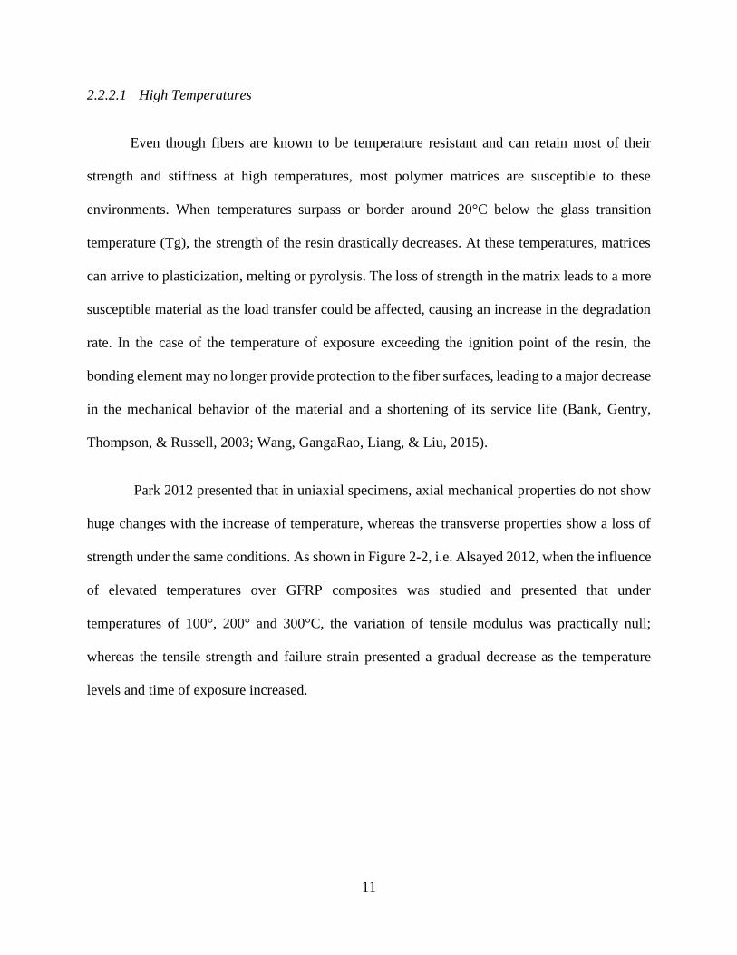
Park 2012 presented that in uniaxial specimens, axial mechanical properties do not show
huge changes with the increase of temperature, whereas the transverse properties show a loss of
strength under the same conditions. As shown in Figure 2-2, i.e. Alsayed 2012, when the influence
of elevated temperatures over GFRP composites was studied and presented that under
temperatures of 100°, 200° and 300°C, the variation of tensile modulus was practically null;
whereas the tensile strength and failure strain presented a gradual decrease as the temperature
levels and time of exposure increased.

12
Figure 2-2-Performance of GFRP bars under elevated temperatures. (a) Tensile strength, (b) Failure strain
and (c) Tensile modulus (Alsayed, 2012).
2.2.2.2 Low temperatures and freeze-thaw cycles
Degradation rates of FRP composites under low temperatures are less than those under high
temperature environments. Nonetheless, cold temperatures and freeze-thaw (FT) cycling can affect
FRP composites due to a differential thermal expansion between the polymeric matrix and the
fiber reinforcements, possibly resulting in a deterioration of the fiber-matrix interface (Wang,
GangaRao, Liang, & Liu, 2015).

13
Robert et al. 2010 test data showcased increased values in their mechanical properties
(tensile, shear and flexural strengths) when the temperature decreased, as presented in Figure 2-3.
This phenomenon occurred due to the increase of stiffness in the amorphous polymer matrix under
low temperatures. The flexural modulus of elasticity appeared to be stable in temperatures between
-40° to +50°C.
(a) (b)
(c) (d)
Figure 2-3-Average mechanical properties of GFRP bar specimens tested under different temperatures:
(a)Tensile strength, (b)Shear strength, (c) Flexural strength and (d) Tensile Modulus (Robert, Wang, Cousin,
& Benmokrane, 2010)

14
When FRPs are subjected to freezing temperatures along with mechanical properties
variations, additional micro-cracks are appreciated in the specimens. This can lead to an increase
in water absorption when temperatures raise. Also, the expansion of water, present in the FRP
structure when subjected to freezing temperatures, can cause the growth of cracks and finally lead
to debonding in the fiber-matrix interface (Wang, GangaRao, Liang, & Liu, 2015).
2.3 Aging prediction models of FRP composites
As stated in GangaRao et al. 2006 and presented in previous sections of this chapter, the rate of
degradation in polymer composites depends on various factors such as:
The chemical and physical structure of polymers
Additives and modifiers
Moisture
Sustained stress or pressure
Temperature
Physical and chemical aging
Etc.
Different environmental exposures as well as the combination of factors mentioned above
show different degradation models. Several degradation models are presented in the literature, but
for the purpose of this research only two have been studied. Both of them are presented in the
following sections and results from following the Arrhenius equation (2-1).

15
2.3.1 Arrhenius Principle
The fundamental assumption behind using the Arrhenius principle is that degradation is
dominated by a mechanism that does not change with time, but degradation rates vary by
temperature. Whereas the degradation mechanism does not change during exposure with neither
time nor temperature. This principle is used to obtain or extrapolate the long-term behavior and
service life prediction of a material following the Arrhenius Equation (2-1), by using the
temperature dependence of the polymer subjected to environmental aging at different temperature
levels (Celina, Gillen, & Assink, 2005) (GangaRao, 2006) (Silva, da Fonseca, & Biscaia, 2014).
𝑘 = 𝐴 ∙ exp (−𝐸𝑎𝑅 ∙ 𝑇
) 𝑜𝑟 ln 𝑘 = ln 𝐴 +−𝐸𝑎𝑅 ∙ 𝑇
(2-1)
In relation to Equation 2-1, the Arrhenius extrapolations are based on the assumption that
the reaction rate 𝑘 controls the degradation process which is proportional to exp (−𝐸𝑎
𝑅∙𝑇), where 𝐸𝑎
is the Arrhenius activation energy, 𝑅 the gas constant (8.314 J/mol-K), 𝑇 the absolute temperature
and 𝐴 the pre exponential factor. Consequently, a plot in a log scale of the reaction rate (k) or the
degradation times (1/k) is expected to show a straight line variation as shown in Figure 2-4 (Celina,
Gillen, & Assink, 2005).

16
Figure 2-4- Example of an Arrhenius plot for temperature- and time-dependent strength retention.
(GangaRao, 2006)
For the extrapolation of long-term behavior, assuming that the Arrhenius time-temperature
relationship is valid for all the temperatures of the tested range, the determination of a time shift
factor (TSF) is needed, as presented in Equation 2-2 where T1 is the temperature chosen as
reference and the T0 the aging temperature of the data which is being shifted.
𝑇𝑆𝐹 = 𝑒𝑥𝑝 [𝐸𝑎
𝑅(1
𝑇0−1
𝑇1)] (2-2)
Although the TSF presented in Equation 2-2 is the most common form in which Arrhenius
type relationships are found, other research studies (i.e. Zou et al. 2011) have presented a variation
of the Arrhenius type relationship in which the TSF variation is presented in terms of the pH of
the solution, as shown in Equation 2-3, where pHr is the pH taken as reference and pH is the pH
1000
100
10
1
3 3.25 3.5 3.75
Tim
e to
reac
h se
lect
ed F
RP s
tren
gth
valu
e (d
ays)
1/T (x103)0K-1
Θ
Θ
Θ
Θ
Θ
Θ
Θ
Θ
Θ
Θ
Θ
ΘΘ
Θ
Θ
Θ
Θ
Θ
Θ
Θ
Θ
Θ
Θ
ΘΘ
Θ

17
of the environment of the aged data that is being shifted. Further details on the Time-Superposition
Principle and the shifts for long term performance will be developed in Chapters 4, 5 and 6.
𝑇𝑆𝐹 = exp[𝐴 ∙ (10−𝑝𝐻 − 10−𝑝𝐻𝑟)] (2-3)
2.3.2 Non-Arrhenius behavior
The accelerated data prevalent in the literature ranges from several months up to a year,
with instances stretching over several years, but a longer extrapolation is needed to obtain actual
degradation formulas. This limited availability of experimental data is the key weakness in the
Arrhenius principle (Celina, Gillen, & Assink, 2005). Optimal data would include curves that
showcase degradations during several decades of a material’s service-life, highlighting the
limitations within the Arrhenius procedure and its applicability to various projects. This argument
is strengthened when several instances of the linear approximation of the Arrhenius plot (Figure
2-4) showed a tendency to produce a curvature in the degradation plot. This occurs when subjected
to several aging agents when different Ea’s, or a variation of the activation energy to create
degradation reactions comes into picture in the degradation process (Celina, Gillen, & Assink,
2005).
The non-Arrhenius behavior is shown as a combination of two or more independent
reactions with individual and independent degradation rates. The different degradation rates are
presented as a curvature change as a function of different reactions from pH, temperature, etc. This
effect is shown as a change in the constant A on the Arrhenius equation to a function of the
simultaneous process taking place (Equation 2-4). The problem when establishing the non-

18
Arrhenius type relationship, is to determine the exact point of curvature change; as well as
determining the function followed by the changing of the constant A.
𝑘 = 𝑓(𝑥) ∙ exp (−𝐸𝑎𝑅 ∙ 𝑇
) 𝑜𝑟 ln 𝑘 = 𝑔(𝑥) +−𝐸𝑎𝑅 ∙ 𝑇
(2-4)
As presented in Equation 2-5, the variation of the Arrhenius type relationship could also
be represented by establishing a function of the various external agents for the activation energy.
Maintaining A as a constant, as presented in the original Arrhenius equation.
𝑘 = 𝐴 ∙ exp (
−𝐸𝑎(𝑥)
𝑅 ∙ 𝑇) 𝑜𝑟 ln 𝑘 = 𝐴 +
−𝐸𝑎(𝑥)
𝑅 ∙ 𝑇
(2-5)
In Figure 2-5, an example presented in Celina et al. (2005) is shown, it can be observed the
double curvature presented coming from two different degradation processes.
Figure 2-5 Example of curve fitting with two degradation process following a non-Arrhenius type relationship
(Celina, Gillen, & Assink, 2005)

19
2.4 Strength reduction factors “ ” for environmental conditions
Civil engineering structures are generally designed for service life of 75 to 100 years.
However, any material used in the design does not maintain the same mechanical properties during
the service life; therefore, it is important to know the degradation rate of materials with time and
the performance rate of the different elements. For FRP elements, determination of degradation
rate becomes a problem as the knowledge on degradation is limited.
The initial characteristics of a material’s properties and specifications are given by
manufacturers without taking into account the long-term effects from environmental exposure.
Due to degradation, the properties of the composite materials must be modified (reduced) to factors
in different types and levels of environmental effect; these factors are referred as knock down or
strength reduction factors, showcasing the retained strength of the specimens for the service life
period.
Obtaining the strength reduction factors is one of the main efforts of ongoing durability
research. The primary issue is gathering data from all the different experimental studies and
categorizing them by design specifications as every researcher applies different test methodologies
due to a lack of durability test standards. When using the same test methodologies, there are huge
variations in the resin type, fiber type, fiber architecture or manufacturing process; characteristics
that may create variations in the strength of the tested specimens (Wang, GangaRao, Liang, & Liu,
2015).

20
For example, as presented in ACI440.1R-06 the design equation for tensile strength is:
𝑓𝑓𝑢 = 𝐶𝐸𝑓𝑓𝑢∗ (2-6)
where
𝑓𝑓𝑢 = design tensile strength of FRP, considering reductions for service environment
𝐶𝐸 = environmental reduction factor, given in Table 2-1 for various fiber type and
exposure conditions
𝑓𝑓𝑢∗ = guaranteed tensile strength of an FRP bar defined as the mean tensile strength of
a sample of test specimens minus three times the standard deviation (𝑓𝑓𝑢∗ = 𝑓𝑢,𝑎𝑣𝑒 − 3𝜎).
Table 2-1 Environmental reduction factor for various fibers and exposure conditions (440.1R-06, 2006)
The design modulus of elasticity as well as that given by the manufacturer is assumed to be
constant. Usually the reduction factors, 𝐶𝐸, are conservative values adopted as a consensus of the
American Concrete Institute (ACI) Committee. The temperature is considered in these values, but
under the assumption that the FRP composite elements are not subjected to a temperature higher
than the glass transition temperature (Tg).

21
Many experts on the subject consider the current codes and values to be conservative, and
therefore consider it necessary that further research adopts a more accurate approach to evaluate
the degradation of the materials.
2.5 Conclusion
The Arrhenius principle was assumed to be the right path to follow when studying the
degradation and durability of FRP composites as the behavior presented by specimens is generally
a logarithmic decay. In this research study, glass reinforced thermosets are studied under different
environments of pH and temperature.
The degradation sets collected from the literature are presented partially in Chapter 3 and
completely in Appendix A and B. In the sets of data, this study will show how the different
temperature and pH levels affect the degradation to the studied materials for tensile, flexure and
interlaminar shear strengths. Highly alkaline environments (pH≈13) are the pH environments of
extreme concern due to the exposure of composites to concrete environments when applied in civil
infrastructure.
22
CHAPTER 3 DATA COLLECTION
In this chapter, the procedure for existing data collection is developed. In addition, different
data correlations are suggested for a more homogeneous source of information. Data collection is
fundamental to this study. The author lacked adequate time to obtain the data of her own in the
lab, therefore the data presented, stems from data available in the literature.
Most of the data comes from previous research studies on durability at West Virginia
University (WVU), as well as other external sources. The only restriction being that the test data
would not be influenced by any external agent other than pH and Temperature.
3.1 Accelerated aging data
3.1.1 Organization of the database
All the accelerated data collected for this study was gathered and organized in a database for
all the different evaluated environments. The general data collection is formed by 196 sets of
degradation curves lasting up to a time period of 18 months. Each of these sets represents 1 to 7
replications and the majority represent asymptotic behavior.
Given the various sources from which the data was obtained, and the many ways in which the
raw content was presented, all the data gathered in this study was converted to percentage of
strength retention of the tested samples. Several test samples witnessed an increase of strength in
the beginning of the aging process. This increase of strength in the initial months has been assumed
to be a result of post curing issues; the correction for these cases is presented in section 3.1.2.
23
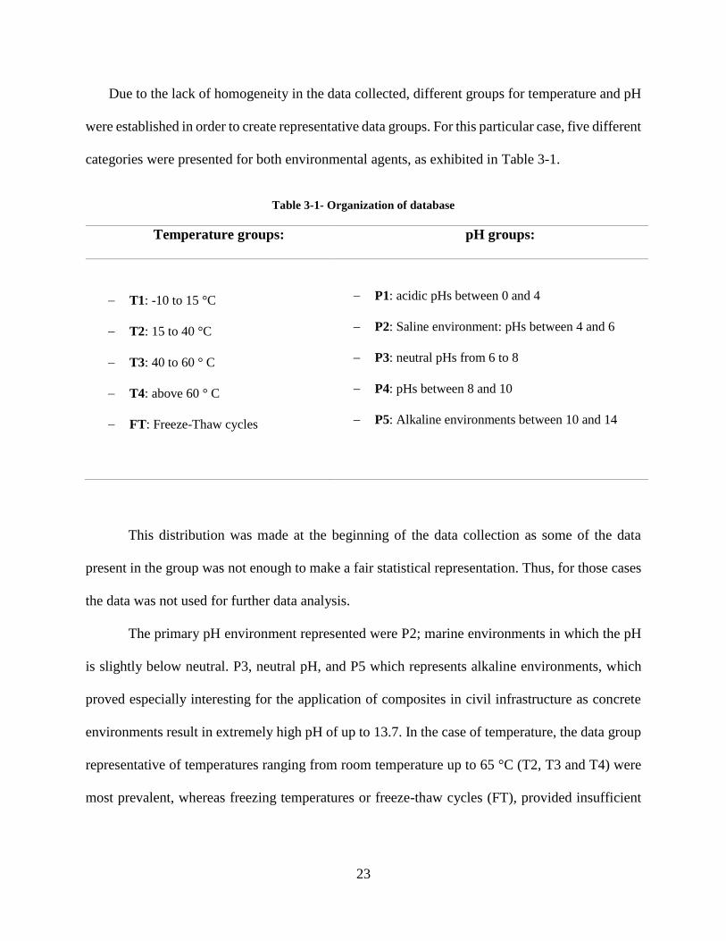
Due to the lack of homogeneity in the data collected, different groups for temperature and pH
were established in order to create representative data groups. For this particular case, five different
categories were presented for both environmental agents, as exhibited in Table 3-1.
Table 3-1- Organization of database
Temperature groups: pH groups:
T1: -10 to 15 °C
T2: 15 to 40 °C
T3: 40 to 60 ° C
T4: above 60 ° C
FT: Freeze-Thaw cycles
P1: acidic pHs between 0 and 4
P2: Saline environment: pHs between 4 and 6
P3: neutral pHs from 6 to 8
P4: pHs between 8 and 10
P5: Alkaline environments between 10 and 14
This distribution was made at the beginning of the data collection as some of the data
present in the group was not enough to make a fair statistical representation. Thus, for those cases
the data was not used for further data analysis.
The primary pH environment represented were P2; marine environments in which the pH
is slightly below neutral. P3, neutral pH, and P5 which represents alkaline environments, which
proved especially interesting for the application of composites in civil infrastructure as concrete
environments result in extremely high pH of up to 13.7. In the case of temperature, the data group
representative of temperatures ranging from room temperature up to 65 °C (T2, T3 and T4) were
most prevalent, whereas freezing temperatures or freeze-thaw cycles (FT), provided insufficient

24
data for the use of this study. The data sets of special concern are presented at the end of this
chapter, but all the collected data is presented in Appendix A.
3.1.2 Correction for post-curing
Curing of resin plays a critical role in the determination of mechanical and chemical properties
of the material. For thermosets, the curing process is an irreversible reaction which is initiated by
heat. In this reaction, the formation of cross links results in a material that is thermally and
mechanically stable (Kumar, et al., 2015).
Since the maximum mechanical properties are achieved when the material has completely
cured, it is possible for the mechanical properties to increase while aging. This is due to the fact
that specimens are not always completely cured at the onset of aging. This test procedure requires
data exhibiting post-curing to be corrected. If the mechanical properties are observed to increase
during aging, this is an indication that the sample has not yet fully cured. The aging process does
not cause these properties to improve. Therefore, data for samples demonstrating increased
strength during aging were adjusted to account for post-curing effects.
In order to make the correction, the maximum strength was determined. The time of the
maximum strength was then established as t0. The data prior to time t0 was then neglected. This
correction is based on the assumption that the aging process does not affect the continuation of
curing up to time t0, at which maximum strength is achieved. An example of a correction in a
sample showing post-curing can be seen in Figure 3-1. Where the max strength was determined to
be 102.5 percent of the initial strength. This strength was achieved after 3 weeks of aging. Thus,
the 3 week time period is taken as t0, and 102.5 percent is taken as the actual 100 percent.

25
Figure 3-1- Example of Post curing correction
3.2 Natural aging data
The collection of naturally aged data was one of the biggest concerns in achieving the
objective of this project. The main limitation when collecting the data, as mentioned before, was
the fact that the samples could not be subjected to any other environmental agent apart from pH
and/or temperature. Within the literature, the bulk of the data available was affected by other
environmental effects, mainly sustained stress as they were samples coming from structures that
had been in service for several years.
The leading source of data for this section stemmed from a previous research conducted at
the Constructed Facilities Center (CFC) at WVU, Dittenber, Gangarao, & Liang, (2016). The
problem with this being that when trying to obtain the strength retention percentages, several
sources (mainly sources external to WVU) did not indicate the initial strength of the material. The
data for which the initial strength was not provided was neglected for the posterior correlation with
the data obtained from lab controlled environments.
85
90
95
100
105
0 2 4 6 8 10
Str
ength
(%
)
time (weeks)
Original data Post curing Correction

26
Another issue emerged when some of the samples showed an increase in the strength of the
aged data, presumably stemming from post-curing problems, as commented before. Considering
the fact that only two points of degradation trends were indicated in the source, there was not an
option to calculate when the post curing reached its maximum and thus, the post-curing correction
presented in section 3.1.2 cannot be applied.
The collected field data is presented in Appendix B and as summary of the obtained data the
degradation curves in Table 3-2.
Table 3-2 Field aging degradation curves
Field degradation curve
Flexural strength y = -3.458ln(x) + 104.14
Tensile strength y = -2.52ln(x) + 102.66
Interlaminar Shear strength y = -4.762ln(x) + 100.39
3.3 Normalization of the accelerated aging data
The data collected lacks homogeneity in terms of the physical characteristics of the
specimens tested. To make up for this inconvenience, a correction on the data obtained in the lab
tests is required. Different corrections could be done in terms of different characteristics of the
manufactured coupons, however in this study only two corrections were made. On the one hand,
different equations were developed for the effect of thickness of the samples and the main
mechanical properties while on the other hand, the effect of the Fiber Volume Fraction (FVF).
Both are extensively developed in sections 3.3.1 and 3.3.2.
For the collected data, the prorating made with a thickness of 1 cm (0.4”) and a FVF of 50
percent.

27
3.3.1 The effect of Fiber Volume Fraction on the strength of the FRP samples
Fiber volume fraction (FVF) is defined as the percentage of the total volume taken by fibers
in a cured fiber reinforced polymer composite. This is a fundamental factor when calculating the
mechanical properties of the material, such as strength or stiffness. An increase of these properties
usually improves the mechanical behavior up to a certain maximum percentage of FVF. Beyond
the max FVF percentage, properties degrade due to inadequate bonding between the fibers and the
polymeric matrix (Siva, 2013).
As stated earlier, the fibers of the FRP composites are assumed to be the major carrier of its
strength, whereas the resin keeps fibers bonded together and provides continuity to the finished
composite. The increase of fiber volume fraction in a composite improves its stiffness and FVF
percent variation changes thermo-mechanical properties. In Figure 3-2, it can be seen how stiffness
keeps increasing as the FVF increases up to certain limit. This increase is approximately linear
until a maximum threshold is reached where it can be seen that the material does not get stiffer
regardless of a higher FVF. However, decrease in the stiffness is found with an increase of the
fiber volume fraction due to inadequate fiber wet-out and lack of adequate shear transfer. This
decrease can be related to a reduction in the bond strength between the resin and fibers (Mini,
Lakshmanan, Mathew, & Mukundan, 2012).

28
Figure 3-2- Variation of Young’s Modulus with volume fraction (Mini, Lakshmanan, Mathew, & Mukundan,
2012).
The strength prediction and correlation with the FVF results were more complicated than
the stiffness (modulus) prediction. Different sources had different statements for the effect of FVF
within the various mechanical properties, and thus the information available was not consistent in
terms of the conditions or characteristics of the samples. In Siva, (2013) ILSS and TS were shown
to increase practically linearly up to 42 percent of FVF. In this research project the strength of the
material was assumed to increase linearly with the FVF. As in Mallick, 2007, assuming that the
fibers in the composite lamina are arranged in a square array, the maximum fiber volume fraction
that can be packed in the arrangement is 78.5%. The maximum FVF presented in the colected data
is a 72%, therefore all the correlated specimens were under the limit at which the mechanical
properties start to decrease.
The correction of the data sets in terms of FVF was made as in Equation 3-1.
𝜎𝑐𝑜𝑟 = 𝜎𝑔𝑖𝑣𝑒𝑛 ∙𝐹𝑉𝐹𝑐𝑜𝑟𝐹𝑉𝐹𝑔𝑖𝑣𝑒𝑛
(3-1)

29
Represented in the formula above:
𝜎𝑐𝑜𝑟 ∶ Strength resulting from prorated conditions
𝜎𝑔𝑖𝑣𝑒𝑛 ∶ Strength given from test results
𝐹𝑉𝐹𝑐𝑜𝑟 ∶ Fiber volume fraction to which the correlation needs to be done
𝐹𝑉𝐹𝑔𝑖𝑣𝑒𝑛 ∶ Fiber volume fraction of the tested samples
3.3.2 The effect of the coupon thickness on the strength of the FRP samples
The theories proposed by Wei-Pin, (1990) have been used for obtaining the influence of
composite thickness on the coupons or bars with both the tensile and bending strengths of the
specimens. A theory has been created for interlaminar shear strength based on the principles
mentioned above with special emphasis on shear lag phenomenon.
It is necessary to clarify that the behavior and responses of composites are complicated to
compute because of different failure modes that the samples may experience under different loads.
Hence a large body of experimental data is needed to validate assumptions and to develop an
accurate prediction theory, as well as for evaluating the process response.
3.3.2.1 Tensile strength
Wei-Pin, (1990) developed a simple relationship between the specimen diameter and the
ultimate tensile strength. The mechanics of materials approach was used in his proposed model,
using three assumptions, given as follows:
i. FRP composite fails when the tensile strain reaches the ultimate fiber strain.
ii. First fiber failure is treated as global failure for design purposes.

30
iii. Strain distribution is parabolic and axisymmetric across the cross-section. The distribution
varies depending on the values of two constants “a” and “b” to be determined with
boundary conditions and experimental data.
𝜀𝑡 = 𝑎 ∙ 𝑟2 + 𝑏 (3-2)
Figure 3-3- Parabolic tensile stress-strain relations assumed. (Wei-Pin, 1990)
Assuming a constant transverse Young’s Modulus along the specimen and that the
maximum value of strain happens in the extreme fibers of a specimen. The tensile strength
distribution ends up being:
𝜎𝑧 =𝐸𝑡2(𝑎𝑅2 + 2𝑏) (3-3)
𝑎 =(𝜀𝑢 − 𝑏)
𝑅2 (3-4)
𝜎𝑧 =𝐸𝑡2(𝜀𝑢 + 𝑏) (3-5)
31
As shown in the equations above, the tensile strength for both circular and rectangular
section coupons result in a linear relationship in terms of the thicknesses of the sample. Leaving
the tensile strengths of the FRP composite to be calculated in terms of “b”. Further details of this
derivation can be found in Wei-Pin’s dissertation (Wei-Pin, 1990).
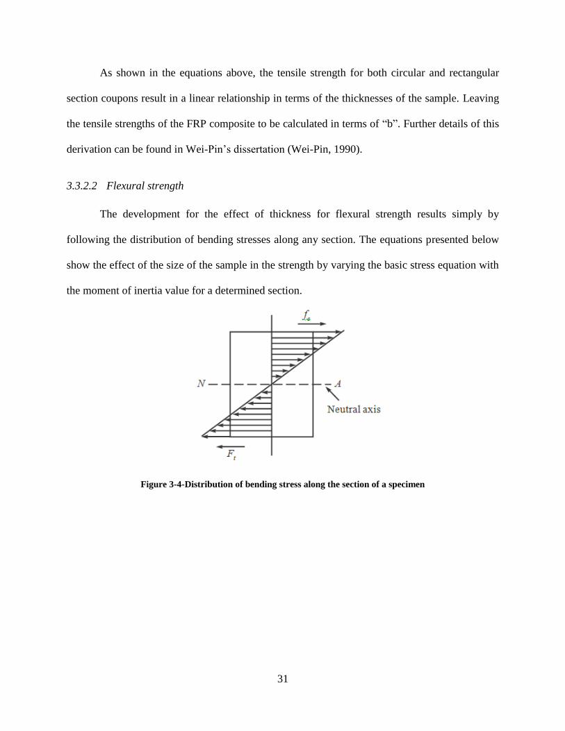
3.3.2.2 Flexural strength
The development for the effect of thickness for flexural strength results simply by
following the distribution of bending stresses along any section. The equations presented below
show the effect of the size of the sample in the strength by varying the basic stress equation with
the moment of inertia value for a determined section.
Figure 3-4-Distribution of bending stress along the section of a specimen

32
RECTANGULAR SECTION CIRCULAR SECTION
𝜎 =𝑀 ∙ 𝑦
𝐼=6 ∙ 𝑀
𝑏 ∙ ℎ2
𝑦 =ℎ
2 ; 𝐼 =
𝑏 ∙ ℎ3
12
(3-6)
𝜎 =𝑀 ∙ 𝑦
𝐼=4 ∙ 𝑀
𝜋 ∙ 𝑟3
𝑦 = 𝑟 ; 𝐼 =𝜋 ∙ 𝑟4
4
(3-7)
In the equations above it is shown how the rectangular section has a parabolic relation (h2),
whereas for the circular section a cubic correction is made.
3.3.2.3 Interlaminar shear strength
For the case of interlaminar shear strength, the three assumptions made for tensile strength
will be taken into account, assuming the FRP composites are transversally isotropic or orthotropic
materials.
{
𝜎𝑥𝑥𝜎𝑦𝑦𝜎𝑧𝑧𝜏𝑥𝑦𝜏𝑥𝑧𝜏𝑦𝑧}
=
[ 𝐶1̅1 𝐶1̅2 𝐶1̅3𝐶2̅1 𝐶2̅2 𝐶2̅3𝐶3̅1 𝐶3̅2 𝐶3̅3
𝐶1̅4 𝐶1̅5 𝐶1̅6𝐶2̅4 𝐶2̅5 𝐶2̅6𝐶3̅4 𝐶3̅5 𝐶3̅6
𝐶4̅1 𝐶4̅2 𝐶4̅3𝐶5̅1 𝐶5̅2 𝐶5̅3𝐶6̅1 𝐶6̅2 𝐶6̅3
𝐶4̅4 𝐶4̅5 𝐶4̅6𝐶4̅5 𝐶5̅5 𝐶5̅6𝐶4̅6 𝐶6̅5 𝐶6̅6]
{
𝜀𝑥𝑥𝜀𝑦𝑦𝜀𝑧𝑧𝛾𝑥𝑦𝛾𝑥𝑧𝛾𝑦𝑧}
(3-8)
𝐼𝐿𝑆𝑆 = 𝜏𝑥𝑧 = 𝐶1̅5 ∙ 𝜀𝑥𝑥 + 𝐶5̅2 ∙ 𝜀𝑦𝑦 + 𝐶5̅3 ∙ 𝜀𝑧𝑧 + 𝐶4̅5 ∙ 𝛾𝑥𝑦 + 𝐶5̅5 ∙ 𝛾𝑥𝑧 + 𝐶5̅6 ∙ 𝛾𝑦𝑧 (3-9)
From the transversely isotropic condition: 𝐶1̅5 = 𝐶5̅2 = 𝐶5̅3 = 𝐶4̅5 = 𝐶5̅6 = 0

33
𝐶5̅5 = 𝐺12 =𝐸1
2 ∙ (1 + 𝜗12) (3-10)
𝜏𝑥𝑧 =𝐸1
2 ∙ (1 + 𝜗12)∙ 𝛾𝑥𝑧 (3-11)
The distribution of the shear stresses are parabolically distributed along the section of the
specimen.
𝛾𝑥𝑧 = 𝑎 ∙ 𝑟2 + 𝑏 ∙ 𝑟 + 𝑐 (3-12)
Figure 3-5- Shear stress distribution on a rectangular section.
Mallick, (2007), indicates what the maximum shear stress value achieved in the center of
a cross section under bending is:
𝜏𝑥𝑧 =3 ∙ 𝑃
4 ∙ 𝑏 ∙ ℎ (3-13)
The equation above shows a linear relation between the maximum strength of the specimen
and the thickness.

34
Figure 3-6- Shear stress distribution in a circular section.
𝜏 =4 ∙ 𝜋
3 ∙ 𝜋 ∙ 𝑅2 (3-14)
On the other hand, and as shown in Figure 3-6, the relation between the maximum strength
of the specimen and the bar diameter is parabolic.
3.3.2.4 Summary
In Table 3-3, the equations to account for the effect of the thickness of the tested specimens
in the strength of the materials are presented.
Table 3-3- Effect of the thickness of the sample in the strength of the material
Tensile Flexure Interlaminar Shear
Circular Section
(Bars)
𝜎𝑐𝑜𝑟𝑟 = 𝜎𝑔𝑖𝑣𝑒𝑛𝑟𝑐𝑜𝑟𝑟𝑟𝑔𝑖𝑣𝑒𝑛
𝜎𝑐𝑜𝑟𝑟 = 𝜎𝑔𝑖𝑣𝑒𝑛 (𝑟𝑔𝑖𝑣𝑒𝑛
𝑟𝑐𝑜𝑟𝑟)3
𝜏𝑐𝑜𝑟𝑟 = 𝜏𝑔𝑖𝑣𝑒𝑛 (𝑟𝑔𝑖𝑣𝑒𝑛
𝑟𝑐𝑜𝑟𝑟)2
Rectangular
Section
𝜎𝑐𝑜𝑟𝑟 = 𝜎𝑔𝑖𝑣𝑒𝑛𝑡𝑐𝑜𝑟𝑟𝑡𝑔𝑖𝑣𝑒𝑛
𝜎𝑐𝑜𝑟𝑟 = 𝜎𝑔𝑖𝑣𝑒𝑛 (𝑡𝑔𝑖𝑣𝑒𝑛
𝑡𝑐𝑜𝑟𝑟)2
𝜏𝑐𝑜𝑟𝑟 = 𝜏𝑔𝑖𝑣𝑒𝑛𝑡𝑔𝑖𝑣𝑒𝑛
𝑡𝑐𝑜𝑟𝑟

35
3.4 Presentation of the prorated data
After the post-curing, thickness and Fiber Volume Fraction corrections were made to all data
sets, the average of the prorated data for the different degradation times was plotted as shown in
the Figures 3-7 and 3-8. In these plots the degradation under different temperatures for a certain
material, mechanical property and pH group can be seen. All the plots are presented in Appendix
A, at this point only the most relevant plots are presented in Figures 3-7 and 3-8. In these figures,
the degradation plots of Interlaminar Shear Strength for Vinyl-ester and Polyester under alkaline
environments are presented. From all the cases studied these two are the ones showing the most
concerning behavior as they present an early dramatic decrease of the materials’ interlaminar shear
strength under the alkaline environment.
It may be noted that these plots display varying degradation patterns, but as in many other
research studies the polyester shows a higher degradation than vinyl-ester. Also, it can be seen in
the figures below that the higher the temperature to which the samples are subjected the higher the
degradation is; a behavior exhibited in the majority of all studies in degradation.
The main concern when achieving this result is the fact that the most common use of GFRPs
in civil infrastructure is reinforcing bars embedded in concrete (which produces a strong alkaline
environment), many of these bars are to a certain extent subjected to shear forces, which lab tests
indicate that under room temperature, the FRP composites experience a reduction of approximately
50-60% in strength for the first 3-4 months of accelerated aging.
In following chapters, how this behavior translates to a longer period of time will be
evaluated by using the time-temperature superposition principle. Correlating with the natural aged
specimens data, the strength reduction factors are obtained following the procedure presented in
Chapter 4.

36
Figure 3-7- Degradation of Interlaminar Shear Strength for Vinyl-ester under alkaline environments
Figure 3-8-Degradation of Interlaminar Shear Strength for Polyester under alkaline environments
0
10
20
30
40
50
60
70
80
90
100
0 50 100 150 200 250 300 350 400 450
ILS
S(%
)
Time(days)
T2
T3
T4
0.00
10.00
20.00
30.00
40.00
50.00
60.00
70.00
80.00
90.00
100.00
0 100 200 300 400 500
ILS
S (
%)
Time (days)
T2
T3
T4

37
CHAPTER 4 METHODOLOGY FOR CORRELATION
BETWEEN ACCELERATED AND NATURAL AGING
In previous chapters, the need for accelerated aging data was addressed and the data available
in the literature was presented. To increase the implementation of new materials, it is necessary to
know the service and aging behavior in the field. For performance durability understanding,
accelerated aging tests were performed under controlled lab environments by many researches. In
this chapter, a methodology is presented to correlate the different environments created in the lab
and the limited data obtained from the field. The correlation is made by applying the Arrhenius
type relationship and following the Time-Temperature superposition principle, and a set procedure
developed herein presented in Chapter 5.
In this research, time dependent stresses at different temperatures for different pH
environments (Saline, Neutral and Alkaline environments) were taken in order to correlate the
accelerated aging data to that of the naturally aged data. The process followed is outlined in Section
4.1.
4.1 Accelerated aging methodology
In addition to recording material behavior under varying chemical and environmental
conditions, resistance factors and degradation curves of different materials are needed as the
composite age under service conditions. It is crucial to understand long-term aging trends and a
range of values of the strength of a material under different conditions. The service life of a
structural element fundamentally determines the service life and performance of a structure.

38
Furthermore, the service life based conditions should be closely examined as they impact the
structural performance. However, as FRP composites are relatively new, a vast amount of data
which covers long term field performance are not yet available in order to establish the strength
reduction factors. To overcome this limitation, an approximate simulation of the lifetime of the
material was established by using lab based accelerated aging techniques. By evaluation of the lab
based simulation, it is possible to simulate field (longer-term) performance of GFRP composites.
The accelerated aging tests mentioned above consist of subjecting the different structural
elements to different levels of temperature and pH solutions for establishing material property
degradation under different conditions. Several lab tests run by other researches [Cabral‐Fonseca,
Correia, Rodrigues, & Branco, 2012; Chen, Davalos, & Ray, 2006; Chin, 2001; Dejke & Tepfers,
2001; Grammatikos, et al., 2016; Hammami & Al‐Ghuilani, 2004; Kajorncheappunngam, 1999;
Karbhari, 2004; Kim, Park, You, & Moon, 2008; Marru, et al., 2014; Rivera, 2002; Robert, Wang,
Cousin, & Benmokrane, 2010; Sen, Mullins, & Salem, 2002; Shi, Zhu, & Wu, 2011; Sonawala,
1996; Vijay P. , 1999; Wang, GangaRao, Liang, & Liu, 2015; Won, Lee, Kim, Jang, & Lee, 2008]
at different time periods measuring the desired mechanical properties and obtaining the
degradation curves for different environments are evaluated. The accelerated aging data is
processed and correlated to naturally aged data. This complete process is done by following the
principles established by Litherland, 1981 and Vijay, 1999 whose principles are summarized in
the steps below:
1. Test specimens need to be prepared for different environments from where the accelerated
aging data is going to be extracted after lab based aging of FRP composites. Usually these
environments are more aggressive compared to in-service structural elements. The factors

39
considered for this research are different variations in pH values, temperature and their
combinations.
2. The prepared specimens are tested and evaluated for different mechanical properties.
Typically, testing is done in previously established time intervals, the time periods in
between each testing should be more frequent at the beginning and could be expanded in
time in later experiments.
This research is based on data available in the literature. Therefore, as presented in Chapter 3,
the data was collected and prorated to meet an arbitrary sample.
3. After collecting the data from literature, the degradation curves for different environments
are created. For these degradation curves, the strength loss has been presented in percentage
of ratio of stress to failure of aged sample to the original stress to failure (strength retention)
versus the time for the different environments. Plots are usually non-linear, typically
presented as logarithmic or asymptotic degradation with the time, as shown in Figure 4-1.
In addition, it is exhibited that the degradation is faster and more severe as the temperature
increases (GangaRao, Taly, & Vijay, 2006).
These plots are obtained after following the process presented in chapter 3. Different
degradation sets after corrections were made (post curing, effect of FVF and the thickness of the
specimen) and are presented in Appendix A, in which it can be seen that the majority of data sets
displayed asymptotic behavior.

40
Figure 4-1- Strength retention of aged FRP at different temperatures
4. Following an Arrhenius type relationship, a replot of the degradation curves is required.
This replotting method transforms the logarithmic curves into linear curves. For each of
the strength retention values (90%, 80%, 70%, etc.), a straight line was fitted for the
logarithm of the time needed to reach that particular strength retention versus the inverse
of temperature. Normalization of Arrhenius plots provides an overall image of the relative
acceleration of the loss of mechanical properties at different temperatures/degradation rate
(GangaRao, Taly, & Vijay, 2006). Lines are, generally, parallel for a perfect strength
degradation-temperature relationship but that may not be the case in normal practice.
As presented in Figure 4-2, the data is plotted with time on the vertical-axis and the
inverse of temperature on the horizontal-axis.
0.00
20.00
40.00
60.00
80.00
100.00
0 100 200 300 400 500
stre
gnth
ret
enti
on
(%)
Time (days)
25°C
45°C
60°C

41
Figure 4-2-An Arrhenius plot for temperature- and time-dependent strength retention
Normalization of the curves plotted in
5. Figure 4-2Normalization of the curves plotted in Figure 4-2, into a single curve. The
normalization is made along the vertical axis relative to a reference temperature. The
normalization procedure starts by selecting the reference temperature (t0). In this research,
room temperature (RT=25°C) was chosen as the reference temperature.
Once the reference temperature is chosen, the time shift factors are obtained to
create the normalized time displacement curve relative to the reference temperature as
shown in Figure 4-3, resulting in longer-term degradation curves of the data obtained from
the lab. Following Equation 4-1, the Time Shift Factors (TSF) are obtained as a ratio of the
degradation time under certain temperatures over the degradation time (up to the same
Strength Retention) under the temperature of reference (Silva, da Fonseca, & Biscaia,
2014; GangaRao H. V., 2006).
10
100
1000
10000
2.9 3 3.1 3.2 3.3 3.4 3.5 3.6
Tim
e to
rea
ch s
elec
ted
FR
P s
tren
gth
val
ue
(day
s)
1/T(x10^3) °K^-1
90%
80%
70%
60%

42
The degradation times for each of the strength retention levels (90%, 80%, 70%,
etc.), are obtained from the degradation curves presented in Figure 4-1. TSF can also be
obtained as a ratio of the slopes presented by Arrhenius plots, resulting in a more tedious
process and less accurate approximation the curves obtained from the lab data are,
generally, not exactly parallel so the variation of the variable “A” in the Arrhenius equation
would need to be taken into account, leading to a slight variation of the results.
Figure 4-3- Normalized time displacement curve (Arrhenius plot) relative to a reference temperature
After arriving to this stage and obtaining the normalized time-displacement curves
relative to the temperature of reference (also referred to as the longer term degradation
curve for the accelerated aging data under the reference temperature), the work of the
accelerated aging data is completed and ready to correlate with the field data, as presented
below.
1
1.2
1.4
1.6
1.8
2
2.2
2.4
2.6
2.8
2.9 3 3.1 3.2 3.3 3.4
TS
F
1/Temperature*1000(°K-1)
𝑇𝑆𝐹 =
𝑡1
𝑡2= 𝑒
𝐸𝑎𝑅(1𝑇2−1𝑇1) (4-1)

43
6. Finally, with the shifted plots obtained previously, the natural aging data correlation can
be made. A similar normalization to that in the various temperatures presented in steps 4
through 6 is made between the accelerated aging data at room temperature and the naturally
aged samples. A good example is presented in Figure 4-4. It should be noted that not
enough data points may be available for naturally aged data under various temperatures. A
calibration with naturally aged data will be necessary to accurately predict strength
reduction under long-term field conditioning.
Using the normalized/calibrated plots, the objective is to predict the loss of mechanical
properties over the natural weathering process. Ideally, prediction for a range in between 10 and
100 years of natural aging is desired to obtain a reliable degradation plot and strength reduction
factors for design purposes. Having such a long period of degradation time from a field degradation
is neither practical nor cost-effective. By following the procedure above, having a shorter field
100
10
1
0.1
3 3.25 3.5 3.75
Tim
e sh
ift r
elat
ive
to t
ime
at a
ref
eren
ce t
emp.
(day
s)
1/T (x103)0K-1
Θ
Θ
Θ
Θ
ΘΘ
Θ
Δ Natuarlly weathered FRPΘ Accelerarted-aged FRP
Δ
Δ
Δ
Δ
Δ
Figure 4-4-Normalized time displacement curve (Arrhenius plot) with natural weathering data (GangaRao,
Taly, & Vijay, 2006).

44
degradation data and correlating it with the data aged in the lab, the long term degradation can be
extrapolated cost-effectively and with less time constraints.
4.1.1 Limitations of the approach
The limitation of this method, is the fact that only one environmental effect is taken into
account to correlate the data. This temperature is taken as the basis of the normalization process
setting aside other effects such as the pH of the solution used for, accelerated aging moisture
absorption, sustained stress to which the structural components could be subjected to or any other
agent that could age a GFRP element (Vijay, 1999).
4.2 Arrhenius plots
Normalize Arrhenius plot provides an overall curve of relative loss of accelerated strength
or stiffness at different temperatures, as shown in Figure 4-2. As noted earlier, the principal
assumption when applying the Arrhenius principle is the degradation mechanism of the materials
which does not change with time, but changes with temperature only. In other words, the behavior
of materials in the long term has one dominant degradation mechanism, i.e. temperature in this
case. Due to this assumption, all temperature regression curves should be presented approximately
parallel, with similar slopes. Otherwise the degradation mechanism is also temperature dependent
(Silva, da Fonseca, & Biscaia, 2014).
As presented in Appendix C, most plots present a good parallel behavior with reference to
temperature. But a few cases have been exhibiting deviation from linear and parallel behavior,
which could be related to the fact that there is pH acting on the temperature exposure (sole variation
as assumed originally), causing deviation to ideal (linear) degradation response to temperature.
Such effect is shown with an example in Figure 4-5, where it is seen that the fit to parallel lines to

45
the neutral pH is consistent whereas for alkaline environments at lower degradations, the strength
retention curves are parallel. At higher degradations however a slight increase in slopes of these
curves are observed.
Figure 4-5-Example of pH effect in the deviation of the Arrhenius plots
4.3 Activation energy
Activation Energy (Ea) is known as the difference between the reactant and the transition
state. In other words, the energy level that the reactants need in order for a reaction to occur.
Figure 4-6- Activation Energy of a reaction
10
100
1000
10000
2.8 3 3.2 3.4 3.6
Tim
e to
rea
ch s
elec
ted
FR
P s
tren
gth
val
ue
(day
s)
1/T(x10^3) °K^-1
VE-ILSS-NEUTRAL PH
10
100
1000
2.8 3 3.2 3.4 3.6Tim
e to
rea
ch s
elec
ted
FR
P s
tren
gth
val
ue
(day
s)1/T(x10^3) °K^-1
VE-ILSS-Alkaline Environment
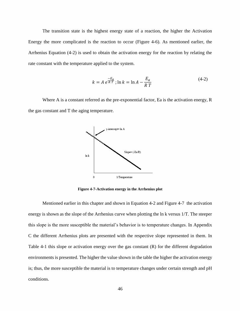
46
The transition state is the highest energy state of a reaction, the higher the Activation
Energy the more complicated is the reaction to occur (Figure 4-6). As mentioned earlier, the
Arrhenius Equation (4-2) is used to obtain the activation energy for the reaction by relating the
rate constant with the temperature applied to the system.
𝑘 = 𝐴 𝑒
−𝐸𝑎𝑅 𝑇 ; ln 𝑘 = ln 𝐴 −
𝐸𝑎𝑅 𝑇
(4-2)
Where A is a constant referred as the pre-exponential factor, Ea is the activation energy, R
the gas constant and T the aging temperature.
Figure 4-7-Activation energy in the Arrhenius plot
Mentioned earlier in this chapter and shown in Equation 4-2 and Figure 4-7 the activation
energy is shown as the slope of the Arrhenius curve when plotting the ln k versus 1/T. The steeper
this slope is the more susceptible the material’s behavior is to temperature changes. In Appendix
C the different Arrhenius plots are presented with the respective slope represented in them. In
Table 4-1 this slope or activation energy over the gas constant (R) for the different degradation
environments is presented. The higher the value shown in the table the higher the activation energy
is; thus, the more susceptible the material is to temperature changes under certain strength and pH
conditions.

47
Table 4-1- Activation Energy values for the different aging processed
Resin Strength pH -Ea/R
VE Tensile
Strength
Neutral pH -0.241
Saline pH (4-6) -0.636
Alkaline (pH=13) 1.301
PE Tensile
Strength
Neutral pH -1.247
Saline pH (4-6) 1.049
Alkaline (pH=13) -
VE Flexure
Strength
Neutral pH -1.139
Saline pH (4-6) 5.178
Alkaline (pH=13) -
PE Flexure
Strength
Neutral pH 0.062
Saline pH (4-6) 2.414
Alkaline (pH=13) -
VE
Interlaminar
Shear
Strength
Neutral pH 4.583
Saline pH (4-6) 5.327
Alkaline (pH=13) 1.983
PE
Interlaminar
Shear
Strength
Neutral pH 2.637
Saline pH (4-6) 0.414
Alkaline (pH=13) 0.964
The lower the activation energy values are, lower temperature is needed for the degradation
to occur, wherein the time shift factor is less dependent on temperature. For higher activation
energy values the time shift factors are more dependent on temperature and the temperature
required for degradation is higher than that at lower values of Ea. The results presented in Table
4-1 are not totally consistent with the theory behind. The results for Interlaminar Shear Strength
(ILSS) are presenting the most accurate fit to the theory, being neutral pH the environment at

48
which the highest activation energy is presented. Thus, for developing the degradation under
neutral environment, the temperature required is the highest between the studied environments
(saline, alkaline and neutral pHs). On the other hand, for alkaline environments it is observed that
half the activation energy is required compared to the neutral environments, showing that the
presence of the alkalinity in the environment could be helping the degradation to happen at lower
temperatures.
When comparing between the behavior of Vinyl-ester (VE) and Polyester (PE) in ILSS, VE
showcases higher values of activation energy than PE. Meaning that, at same temperature, the
degradation is less likely to happen in VE than in PE, consistent results with those presented in
Chapter 3 and Appendix A.
The values for activation energy can be used to determine predominant failure mechanisms
under various environments. While models for these predictions have not yet been employed, these
failure modes can be determined through comparison of the durability behavior between neat resin
coupons and reinforced polymers. This comparison is needed under the assumption of the
degradation of GFRP composites being predominantly due to degradation of the matrix or the
fiber-matrix interface and not due to degradation of the reinforcing fibers.
4.4 Conclusions
The methodology adopted in the research has been presented. The different steps are
presented for obtaining long term extrapolation of the behavior of FRP materials in the field by
correlating the acceleratedly aged data obtained in the lab in several months, with the sparsely
available data from the field over several years. This full process is developed in more detail with
the data obtained from the literature in Chapters 5, 6 and Appendices C and E .

49
In the following chapter, a relationship is obtained between temperature and pH to which
the materials were exposed and the Time Shift Factors, closely related to the activation energy. By
establishing this relationship in case of having other test data, a quick shift of the new data could
be made, avoiding the tedious process presented in Chapter 4.

50
CHAPTER 5 TIME-TEMPERATURE SUPERPOSITION
Most durability studies take place in controlled laboratory environments where the
specimens are subjected to different controlled temperatures, allowing researchers to obtain a long-
term degradation of subjected specimens in a relatively short period of time by using the Time-
Temperature Superposition (TTS) principle. Such a principle, developed earlier by many authors
(i.e. Van Gurp, 1998; GangaRao et al, 2006) has been elaborated in this chapter.
5.1 Time-temperature stress superposition principle
The Time-Temperature Superposition (TTS) principle is predominantly used to establish the
behavior of materials under different mechanical properties for longer periods of time than the
time used to obtain the original data obtained from the lab. By shifting the behavior of the samples
at different temperatures to a referenced temperature, an extrapolation of the degradation plots can
be obtained (Van Gurp, 1998). For example, by performing accelerated aging test in the span of
18 months in the lab under different environments and applying the TTS principle, up to 45 years
of degradation in the field can be extrapolated.
The strength retention and other properties, i.e. stress relaxation modulus (Figure 5-1), of a
polymer composite measured over time under a certain temperature, may be used to relate
approximately the behavior of a material’s properties under other temperatures. This principle is
generally known as the Time-Temperature Superposition principle and is employed to correlate or
calibrate naturally aged results of FRPs at ambient temperatures with results from acceleratedly
aged specimens (GangaRao, Taly, & Vijay, 2006), implying that the behavior at one temperature
can be related to that at another temperature by a change in the time-scale only (Ward, 2004).

51
This principle is only applicable under the conditions in which the materials are stable and
those that do not change the rheological measurements. For example, the TTS is not applicable for
temperatures around the glass transition temperature of the polymers (Van Gurp, 1998).
Figure 5-1- Construction of a master curve for the stress relaxation modulus at 25°C reference temperature
(Strobl, 1997)
5.2 Time shift factors
Time shift factors (TSF) allow one to normalize the degradation rates of specimens under
different environmental into a single time-scale. After the TSF is obtained, the activation energy
is calculated and the regression curves can be applied to predict strength retention for natural aging
conditions.
5.2.1 Time shift factors vs. temperature
By using an Arrhenius type relationship in the degradation trends in terms of temperature,
and as found in Silva el at. 2014 “the time shift factor (TSF) is defined as the ratio between the

52
times required for a certain decrease in a mechanical property at two different temperatures”, as
shown in Equation 5-1.
𝑇𝑆𝐹 =𝑡1𝑡2=𝐴 ∙ 𝑒
𝐸𝑎𝑅(1𝑇2)
𝐴 ∙ 𝑒𝐸𝑎𝑅(1𝑇1)= 𝑒
𝐸𝑎𝑅(1𝑇2−1𝑇1) (5-1)
Represented in the equation above, t1 is the time it takes to achieve certain degradation at
temperature T1, and t2 is the time to arrive to that same degradation at T2 (where T2 is the
temperature of reference).
Table 5-1 Example to obtain Time Shift Factors for Vinyl-ester under Interlaminar Shear Strength and
Alkaline pH (T2: 25°C-temperature of reference, T3:45°C, T4:60°C)
Degradation times (days) Time shift factors
T2 T3 T4
T2 T3 T4
90% 20 12 11.25 TSF 90% 1 1.67 1.78
80% 40 20 22.5 TSF 80% 1 2 1.78
70% 60 35 33.75 TSF 70% 1 1.71 1.78
60% 85 50 45 TSF 60% 1 1.7 1.89
50% 150 60 56.25 TSF 50% 1 2.5 2.67
40% 300 75 67.5 TSF 40% 1 4 4.44
TSF (Average) 1 2.263 2.389
In Table 5-1, an example to explain how to obtain the TSF is presented using Equation 5-
1. Firstly, the time of degradation for each strength retention level (90%, 80%, 70%, etc.) is
extracted from the degradation plots (Appendix A). Using Equation 5-1, TSF for each strength
retention level is defined by the ratios of time “t1” at certain temperature to achieve the strength
retention level over that time “t2” at the temperature of reference to arrive to that same strength
retention level (i.e. 90% ,80% ,70% , etc.). The TSF values presented in Table 5-2 are the averages

53
of the TSF for all the different strength retention levels for acceleratedly aged specimens. The
average TSF value shown as TSF (Average) is used to extrapolate plots for another temperature to
the reference temperature.
The room temperature (25°C) was taken as reference of temperature for this research,
therefore the TSF for that temperature remains constant in every case, as unity. Given that at higher
temperatures (always remaining under the glass transition temperature to apply the TTS principle)
the degradation rates are higher, the TSF theoretically increase with temperature. The fact that
degradation increases with temperature leads to TSFs greater than one (>1) when temperature is
higher than the reference. However, the results obtained are not always consistent with this TTS
theory. In some of the TSFs presented in Table 5-2 it can be observed that certain values are below
unity which means that the degradation at that temperature is less than at the temperature of
reference. Given that the temperature of reference is the lowest temperature presented the fact that
the degradation is faster under 25°C would not follow the theory behind. Varied reasonings could
explain the numbers exhibited in Table 5-2. For example, the effect of pH is not taken into account
when applying the Time-Temperature Superposition principle. However, the aging effect of pH
levels (to which the samples are subjected to) could explain the disparity of results to some extent.
In addition, variations in the manufacturing processes may also affect the test data. Studies used
in this report did not provide enough details about the manufacturing process employed, which
also led to a wide-spread variation of the strength retention during the accelerated aging process.

54
Table 5-2- Time Shift Factors for acceleratedly aged samples coming from lab controlled environments
Resin Strength pH
Time Shift Factors
T=298ºK T=318ºK T=333ºK
VE
Tensile
Strength
Neutral pH 1.0 0.3 0.9
Saline pH (4-6) 1.0 - 0.9
Alkaline(pH=13) 1.0 - 10.4
PE
Tensile
Strength
Neutral pH 1.0 1.2 1.4
Saline pH (4-6) 1.0 1.4 0.6
Alkaline(pH=13) - - -
EX
Tensile
Strength
Neutral pH - - -
Saline pH (4-6)) 1.0 1.2 1.7
Alkaline(pH=13) 1.0 1.2 3.0
VE
Flexural
Strength
Neutral pH 1.0 2.4 6.5
Saline pH (4-6) 1.0 1.3 0.6
Alkaline(pH=13) - - -
PE
Flexural
Strength
Neutral pH 1.0 1.0 0.8
Saline pH (4-6) 1.0 2.2 0.9
Alkaline(pH=13) - - -
VE
Interlaminar
Shear
Strength
Neutral pH 1.0 3.5 6.6
Saline pH (4-6) 1.0 2.4 5.1
Alkaline(pH=13) 1.0 2.3 2.4
PE
Interlaminar
Shear
Strength
Neutral pH 1.0 1.1 1.2
Saline pH (4-6) 1.0 1.9 2.6
Alkaline(pH=13) 1.0 1.5 1.7
55
5.2.2 TSF -temperature relationship
It is important to obtain the relationships between TSF and temperature in order to obtain
time shift factors to avoid the tedious process of obtaining Arrhenius plots. It is observed that the
relationship between the TSF and the inverse of temperature (1/T) should fit in an exponential
relationship. The obtained equations for the TSF versus Temperature relationships are presented
in Table 5-3 and the plots shown in Appendix D. In these plots, it is noticed that the R2 values exist
as two extremes: either values above 90 percent (i.e. polyester under tensile strength and neutral
pH, vinyl-ester under flexure and neutral pH, and both vinyl-ester and polyester under shear and
all pH variations) or almost null values (i.e. vinyl-ester under tensile strength and both neutral and
saline pHs or polyester under flexural strength and saline pH). Showing that the relationship
between TSF and Temperature is either highly accurate fitting in an exponential curve or highly
inaccurate. Correcting these values is difficult due to the narrow range of data available for
obtaining these relationships.
Overall the best fits were obtained for Interlaminar Shear Strength (ILSS) related time shift
factors, as presented in Figures 5-2 and 5-3 .

56
Figure 5-3 TSF versus temperature relationship for Polyester under interlaminar shear strength
y = 3.9678e-0.409x
R² = 0.9623y = 9903.6e-2.736x
R² = 0.9936
y = -1.8945x + 7.3915
R² = 0.9537
0
0.5
1
1.5
2
2.5
3
2.95 3 3.05 3.1 3.15 3.2 3.25 3.3 3.35 3.4
TS
F
1/Temperature*1000(°K-1)
TSF vs T° PE-ILSS
Neutral pH Lower pH (4-6)Alkaline (pH=13) Expon. (Neutral pH)Expon. (Lower pH (4-6)) Linear (Alkaline (pH=13))
y = 8E+07e-5.413x
R² = 0.9953
y = 5E+06e-4.597x
R² = 0.9943
y = 6173.4e-2.578x
R² = 0.879
0
1
2
3
4
5
6
7
8
2.95 3 3.05 3.1 3.15 3.2 3.25 3.3 3.35 3.4
TS
F
1/Temperature*1000(°K-1)
TSF vs T° VE-ILSS
Neutral pH Lower pH (4-6)Alkaline (pH=13) Expon. (Lower pH (4-6))Expon. (Alkaline (pH=13))
Figure 5-2 TSF versus temperature relationship for Vinyl-ester under interlaminar shear strength

57
Table 5-3- TSF vs Temperature Relationship for samples coming from lab controlled environments
Resin Strength pH TSF vs T relationship
(y=TSF & x=1/T*1000)
VE Tensile
Strength
Neutral pH y = 0.055e0.7733x
R² = 0.0409
Saline pH (4-6) y = 0.3068e0.3177x
R² = 0.0482
Alkaline (pH=13)
y = 5E+09e-6.644x
R² = 1
(only two data points)
PE Tensile
Strength
Neutral pH y= 24.987e-0.964x
R² = 0.9562
Saline pH (4-6) y = 0.0181e1.2449x
R² = 0.2721
Alkaline (pH=13) -
VE Flexural
Strength
Neutral pH y = 4E+07e-5.224x
R² = 0.9806
Saline pH (4-6) y = 0.0323e1.0634x
R² = 0.2893
Alkaline (pH=13) -
PE Flexural
Strength
Neutral pH y = 0.1251e0.6308x
R² = 0.6465
Saline pH (4-6) y = -0.2227x + 2.0776
R² = 0.003
Alkaline (pH=13) -
VE Interlaminar
Shear
Strength
Neutral pH y = 8E+07e-5.413x
R² = 0.9953
Saline pH (4-6) y = 5E+06e-4.597x
R² = 0.9943
Alkaline (pH=13) y = 6173.4e-2.578x
R² = 0.879
PE Interlaminar
Shear
Strength
Neutral pH y = 3.9678e-0.409x
R² = 0.9623
Saline pH (4-6) y = 9903.6e-2.736x
R² = 0.9936
Alkaline (pH=13) y = -1.8945x + 7.3915
R² = 0.9537

58
5.2.3 Time Shift Factors vs. pH
As presented in section 5.2.1, the effect of pH is perceived to have certain influence when
obtaining the relationship between time shift factor and temperature. However, this influence is
complicated to formulate because of the overlapping influences of different temperatures and
acidity/alkalinity of solutions.
For this study, the shift in terms of pH was not performed as the degradation under saline,
alkaline and neutral environments were studied, separately. In the case where the accelerated data
needs to be shifted in terms of pH effect, Equation (5-2) may be helpful which uses neutral pH
(=7) as a reference.
𝑎𝑝𝐻 = 𝑎0𝑇 [1 −𝑎𝑏𝑠|7 − 𝑝𝐻|
7] 𝑒𝑥𝑝 [
−∆𝐸𝑅 (1 −
𝑎𝑏𝑠|7 − 𝑝𝐻|7 )
𝑇] (5-2)
5.3 Shift of the accelerated aging data for long term degradation trends
Using the time-temperature superposition principle, the prorated data presented in Chapter
3 was shifted (normalized) to obtain a longer time base as compared to those obtained from the
lab. The increase of the duration of the new degradation trends is computed as a multiplication of
TSF with the original data sets (Equation 5-3).
𝑡𝑠ℎ𝑖𝑓𝑡 = 𝑡𝑜𝑟𝑖𝑔𝑖𝑛𝑎𝑙 ∙ 𝑇𝑆𝐹 (5-3)
All shifted data sets are presented in Appendix E, representing the degradation curves as
shown in Table 5-4. These degradation curves indicate a logarithmic degradation showing different

59
values for the coefficient of determination (R2). Maximum values of R2 are desired for the
degradation curves, though originally some of the values presented were as low as 20 percent.
After in depth evaluation of the degradation data, some of the points were assumed to be bad test
data. After neglecting the defective data, a minimum R2 value of 43 percent was found, with an
average R2 value of 68 percent.
In Figures 5-4 and 5-5, the plots of degradation curves are presented for vinyl-ester and
polyester respectively. Both polyester and vinyl-ester show similar behavior under normal
condition. With regards to the extreme environments (dramatic degradation), the strength retention
of Vinyl-ester is higher. As previously stated in this report, Interlaminar Shear Strength (ILSS) is
showing the highest degradation rate; as can be noted in the degradation plots presented in Table
5-4 and Figures 5-4 and 5-5. In Figures 5-4 and 5-5 the graphic representation of the degradation
curves is presented, to have the whole scatter of obtained data refer to Appendix E. For vinyl-ester,
the most detrimental values of ILSS degradation under alkaline environment, indicating a strength
retention as low as 26 percent after conditioning for 1.5 years in the lab. Similarly, ILSS
degradation for polyester under alkaline environment has the most dramatic strength reduction -
presenting a strength retention of 17 percent after conditioning for 1.5 years in the lab.
The results presented may seem dramatic, but it is important to note that accelerated aging
is not a direct representation of the behavior of the material in the field. Without a correlation (as
given in Chapter 6) between the acceleratedly and naturally aged data, it is difficult to have a good
grasp of aging behavior in the field applications.

60
Table 5-4- Degradation curves for accelerated aging data coming from lab controlled environments, for
different resins, mechanical properties and pH environments
Resin, Mechanical Property & Environment Degradation curve
VE-FS
Saline Env. y = -2.398ln(x) + 89.67
R² = 0.6544
Neutral Env. y = -3.088ln(x) + 96.623
R² = 0.6682
Alkaline Env. y = -5.183ln(x) + 95.696
R² = 0.9099
PE-FS
Saline Env. y = -2.411ln(x) + 98.388
R² = 0.7599
Neutral Env. y = -3.024ln(x) + 91.418
R² = 0.5147
Alkaline Env. y = -10.99ln(x) + 95.82
R² = 0.7949
VE-ILSS
Saline Env. y = -3.218ln(x) + 95.007
R² = 0.453
Neutral Env. y = -3.075ln(x) + 93.477
R² = 0.4599
Alkaline Env. y = -15.24ln(x) + 122.38
R² = 0.8978
PE-ILSS
Saline Env. y = -5.021ln(x) + 95.084
R² = 0.4324
Neutral Env. y = -6.992ln(x) + 83.9
R² = 0.654
Alkaline Env. y = -11.4ln(x) + 89.288
R² = 0.9389
VE-TS
Saline Env. y = -5.243ln(x) + 94.317
R² = 0.7358
Neutral Env. y = -3.485ln(x) + 87.566
R² = 0.6805
pH:8-10 y = -4.292ln(x) + 101.69
R² = 0.8403
Alkaline Env. y = -5.435ln(x) + 93.573
R² = 0.6142
PE-TS
Saline Env. y = -3.094ln(x) + 94.634
R² = 0.5934
Neutral Env. y = -3.704ln(x) + 90.273
R² = 0.6149

61
Figure 5-4-Degradation curves for accelerated aging data related to Vinyl-Ester
0 50 100 150 200 250
0
10
20
30
40
50
60
70
80
90
100
time (days)
Ste
ngth
ret
enti
on (
%)
VINYL-ESTER
ACCELERATION AGED DATA Degradation Curves
VE-FS-SALINE VE-FS-NEUTRAL VE-FS-ALAKINE
VE-ILSS-SALINE VE-ILSS-NEUTRAL VE-ILSS-ALKALINE
VE-TS-SALINE VE-TS-NEUTRAL VE-TS-PH=8-10
VE-TS-ALKALINE

62
Figure 5-5-Degradation curves for accelerated aging data related to Polyester
0 50 100 150 200 250
0
10
20
30
40
50
60
70
80
90
100
time (days)
Ste
ngth
ret
enti
on (
%)
POLYESTER
ACCELERATION AGED DATA Degradation Curves
PE-FS-SALINE PE-FS-NEUTRAL PE-FS-ALKALINEPE-ILSS-SALINE PE-ILSS-NEUTRAL PE-ILSS-ALKALINEPE-TS-SALINE PE-TS-NEUTRAL

63
CHAPTER 6 ANALYSIS OF THE CORRELATION BETWEEN
FIELD AND ACCELERATED AGING DATA
Ideally, one would like to use aging data of FRP composites obtained from accelerated aging
experiments to predict degradation behavior of naturally aged components because of time and
cost factors. Validity of this approach can be examined by comparing data obtained from testing
the field samples with the predictions made from accelerated aging experiments and analysis.
Though plenty of accelerated aging data is available as presented in previous chapters,
obtaining the field or naturally aged data are the major issues, as majority of the field aged samples
stem from structures in service. As one can imagine, aging conditions for in-service structures can
be significantly different from accelerated aging conditions. For example, in-service structures are
subjected to certain amount of sustained stress and occasionally, UV radiation as a result of
exposure to the Sun and undergo temperature and humidity cycling with the changes in weather.
In contrast, for accelerated aging tests reported here, temperature, pH and humidity were carefully
controlled and kept constant while sustained stress and UV exposure were absent. Therefore, most
of the data available in the literature could not be used to correlate field data with lab data for this
study. Only useful field data was obtained from Dittenber et al., 2016 where mechanical properties
were evaluated after 5 to 22 years of aging. These data are exclusively for glass reinforced vinyl-
ester under an environment with neutral pH and room temperature. Furthermore, only two points
of data on time scale - one fresh samples and other after several years of aging are available as
shown in Appendix B. Data during the early part of aging process are not available which are most
useful for performing time-temperature shift analysis. Nonetheless, this data was used to develop
degradation curves for naturally aged composite samples. Figure 6-1 shows degradation curves for

64
lab and field data. Table 6-1 shows corresponding logarithmic expressions relating % retention to
aging time in days. As one can see that there is poor correspondence between the accelerated and
naturally aged behavior. This can be expected since the data under field aging (natural) is
extremely limited and as has been shown in previous chapters, the accelerated aging data has lot
of spread in values particularly under longer time exposures.
Table 6-1 Field and Accelerated aging degradation curves for Glass reinforced Vinyl-ester in Neutral pH and
Room Temperature conditions
Field degradation curve* Accelerated aging curves
Flexural strength y = -3.458ln(x) + 104.14 y = -3.088ln(x) + 96.623
Tensile strength y = -2.52ln(x) + 102.66 y = -3.485ln(x) + 87.566
Interlaminar Shear strength y = -4.762ln(x) + 100.39 y = -3.075ln(x) + 93.477
*only two data points are used
However, to correlate the accelerated and field aging presented above, a similar procedure as
that used to correlate the accelerated aging data based on Time-Temperature Superposition (TTS)
principle can be utilized. As presented in Table 6-1, the degradation curves can be represented by
semi-logarithmic expressions relating % retention with aging times in days. Thus, it can be
proposed that similar expressions as represented by Equations 6-1 and 6-3 can be used to express
degradation curves for field and lab environments, respectively, assuming that theoretically at the
beginning of aging (t = 0 days) the strength retained by the GFRP samples is total (𝜎𝑟𝑒𝑡𝑒𝑛𝑡𝑖𝑜𝑛 =
100%). Then in Equation 6-5, the TSF for these correlations is defined as the time taken by a
specimen in the field to achieve a determined strength retention level (Equation 6-2), over the time

65
it would take the same sample to arrive to that same strength retention level under accelerated
aging (Equation 6-4).
For naturally aged data:
𝜎𝑛𝑎𝑡 = 𝑎 ln(𝑡𝑖𝑚𝑒𝑛𝑎𝑡) + 𝑏 ln(𝑡𝑖𝑚𝑒) + 𝑏 (6-1)
or, 𝑡𝑖𝑚𝑒𝑛𝑎𝑡 = 𝐴 exp (𝜎𝑛𝑎𝑡−𝑏
𝑎) (6-2)
For acceleratedly aged data:
𝜎𝑎𝑐𝑐 = 𝑐 ln(𝑡𝑖𝑚𝑒𝑎𝑐𝑐) + 𝑑 ln(𝑡𝑖𝑚𝑒) + 𝑑 (6-3)
or, 𝑡𝑖𝑚𝑒𝑎𝑐𝑐 = 𝐴 exp (𝜎𝑎𝑐𝑐−𝑑
𝑐) (6-4)
𝑇𝑆𝐹 =
𝑡𝑛𝑎𝑡𝑢𝑟𝑎𝑙𝑡𝑎𝑐𝑐𝑒𝑙𝑒𝑟𝑎𝑡𝑒𝑑
(6-5)
Now two different approaches are presented to obtain the TSF to correlate accelerated with
naturally aging of GFRP specimens. In the first approach the exact values retrieved from the
degradation equations are used. In the equation presented in Table 6-1 “b” and “d” (constants of
the logarithmic equation for the natural and accelerated aging curves, respectively) are not 100,
but suffered a slight variation due to the data obtained from the literature and the applied
corrections. In second approach, an approximation where the theoretical values of “b” and “d”
(𝑏 = 𝑑 = 100 %) are taken. An expression for TSF can be obtained by combining equations 6-

66
1to 6-5which is given as Equation 6-6. Equation 6-6 can be further simplified to Equation 6-7 if b
and d are taken to be 100.The comparison between the TSF for the two approximations is presented
in Table 6-2. It can be seen that the approximation is reasonably close to the exact values, with a
maximum variation of 9.6 percent.
𝑇𝑆𝐹 =𝑡𝑛𝑎𝑡𝑢𝑟𝑎𝑙
𝑡𝑎𝑐𝑐𝑒𝑙𝑒𝑟𝑎𝑡𝑒𝑑=exp (
𝑦 − 𝑏𝑎 )
exp (𝑦 − 𝑑𝑐 )
= exp (𝑎𝑑 − 𝑐𝑏 + 𝑦 (𝑐 − 𝑎)
𝑎𝑐)
(6-6)
𝑇𝑆𝐹 ≅ exp (
(𝑦 − 𝑏) (𝑐 − 𝑎)
𝑎𝑐) (6-7)
Table 6-2 TSF for the accelerated aged and field data correlation
Approximation Exact
Strength
Retention (%) ILSS FS TS ILSS FS TS
Tim
e S
hif
t F
act
ors
100 1.0 1.0 1.0 1.1 1.0 1.0
90 3.2 1.4 3.0 3.5 1.4 3.1
80 10.0 2.0 9.0 11.1 2.0 9.2
70 2.8 2.9
Average 4.7 1.8 4.3 5.2 1.8 4.4

67
60
65
70
75
80
85
90
95
100
0 100 200 300 400 500 600 700 800
Str
enght
Ret
enti
on (
%)
Time (days)
Acc. vs. Nat. aged data for
Vinyl-ester in Neutral pH
VE-TS-lab VE-ILSS-lab VE-FS-lab
VE-FS Acc VE-ILSS Acc VE-TS Acc
VE-FS Field VE-ILSS Field VE-TS Field
Figure 6-1 Accelerated and natural aged samples degradation plots for vinyl-ester under neutral pH

68
Figure 6-2 Predictions for naturally aged data using accelerated aging data and time shift factors for vinyl-ester under neutral pH
60
65
70
75
80
85
90
95
100
0 100 200 300 400 500 600 700 800
Str
enght
Ret
enti
on (
%)
Time (days)
Acc. vs. Nat. aged data correlation for
Vinyl-ester in Neutral pH
VE-FS Natural Long Term VE-ILSS Natural Long Term VE-TS Natural Long Term

69
Degradation vs time curves using the approach previously presented are shown in Figure
6-2 by correlating natural aging data with acceleratedly aged data, previously presented in Table
6-1 and Figure 6-1. It should be noted that this data is applicable only for long-term degradation
of glass reinforced vinyl-ester composites under neutral pH and room temperature and must be
used as an example of applicability of the proposed approach.
Equations 6-1 and 6-4 can be combined to obtain Equation 6-8 which shows that the
strength retention under natural aging follows the same trend with respect to time as the accelerated
aging samples but at a different time scale, where the time under natural degradation equals to TSF
multiplied by accelerated aging time as expressed in Equation 6-9.
𝜎𝑛𝑎𝑡 = 𝑎𝑎𝑐𝑐 ln(𝑇𝑆𝐹 𝑡𝑖𝑚𝑒 𝑎𝑐𝑐) + 𝑏𝑎𝑐𝑐 = 𝑎𝑎𝑐𝑐 ln(𝑇𝑆𝐹 𝑡𝑖𝑚𝑒 𝑎𝑐𝑐) + 100 (6-8)
𝑡𝑛𝑎𝑡 = 𝑇𝑆𝐹 𝑡𝑎𝑐𝑐 (6-9)
However, it can be noted that the TSF obtained and presented in Table 6-2 appear to be
smaller than the values normally presented in literature for the correlation between acceleratedly
and naturally aged samples. From the TSF values obtained, it may be said that a day of accelerated
aging in the lab corresponds to 1.8 to 4.7 days of degradation in the field. In some research studies
(for example, Vijay, 1999) TSF values as high as 30 are exhibited. This implies that undergoing
18 months of exposure in lab under controlled environments (as the ones presented in this research)
would lead to an extrapolation of 85 months (7 years) of degradation in the field for a TSF of 4.7.
Whereas using TSFs ≈30, 540 months (45 years) of degradation in the field could be extrapolated
with the same amount of data from the lab.

70
The major limitation in relating the long term natural degradation from field data to
accelerated aging laboratory data is that: accuracy in obtaining the time shift factors at early
periods of exposure to pH or temperature and consequent degradation cannot be obtained due to
the lack of detailed data available from the naturally aged samples in their early service life. For
example, the field data obtained from the tested samples in the study by Dittenber et al 2016, the
second data point was recorded after 12 years of aging where the specimens would have arrived at
the plateau zone of the semi-logarithmic curve, but the degradation curve during the early years is
missing but which is most crucial for determining the time shift factors for the correlation. For
more accurate results, property measurements during natural aging tests should be conducted more
often during the initial aging stage as the degradation rates are generally higher and the degradation
rates plateau out as time advances. A recommended testing procedure is presented in section 7.5
showing recommended testing times. Having the data of the degradation at early aging in a natural
environment will allow us to obtain a better correlation with the accelerated aging data so that
better prediction about the TSF can be made.
With only two data points for natural aging and the correlation presented in this chapter,
the strength retentions obtained for the long-term field data are as presented in Table 6-3. For a
100 year design service life, the strength retention presented by vinyl-ester samples under neutral
pH is of 66 percent for flexural strength, 63 percent for interlaminar shear strength and 58 percent
for tensile strength. Without taking into account the statistical variability of the data and the fact
that the correlation is made only from two data points of natural aging, the strength reduction
factors to calculate the design nominal strength (Equation 6-10) are presented in Table 6-4.
𝜑 ∙ 𝑅 ≥ 𝛾 ∙ 𝑄 (6-10)

71
Table 6-3 Estimated strength retention in the field for Vinyl-ester and neutral pH after correlation between
acceleratedly and naturally aged data
Strength retention in the field (%)
time
(years) VE-FS VE-ILSS VE-TS
5 75 72 69
10 73 70 66
25 70 67 63
50 68 65 61
75 67 63 59
100 66 63 58
Table 6-4 Estimated strength reduction factors for Vinyl-ester under neutral pH and a 100 year design
service life
Strength Reduction
Factor “φ”
Flexural Strength 0.65
Interlaminar Shear
Strength 0.60
Tensile Strength 0.58
From the analysis above it can be concluded that there is a critical need for the collection
of more natural aging data particularly during the early stages of aging to develop better
correlations and validate the TSF approach. Additional limitations and needs are identified in
Chapter 7.
72
CHAPTER 7 CONCLUSIONS AND RECOMMENDATIONS
7.1 Summary
With the constant evolution of technology, new and advanced materials such as Fiber
Reinforced Polymer (FRP) composites are continuously being developed as structural materials
and systems. In recent years, the demand to substitute conventional construction materials such as
steel or concrete with more advances in materials has grown, for both the new construction and
rehabilitation. This growth is a product of the improved thermomechanical characteristics that
composite materials offer compared to conventional counterparts. Nonetheless, FRP composites
are also susceptible to degradation under both physical and chemical aging. For the increased
implementation of these materials in design, it is important to enhance knowledge base (behavior,
aging, design, etc.) of FRP composites so that they withstand at least 75 to 100 years of service
life.
For a more optimal research of the behavior of FRPs under harsh environments, several tests
were conducted after weathering in lab controlled environments under different temperatures and
pH solutions. Following the proposed correlation between the acceleratedly aged samples in the
lab with data originating from field conditioned samples, a procedure to establish long-term
degradation trend(s) is suggested. The method employed to obtain the correlation proposed in this
thesis was presented first in Litherland et al. (1981) and Vijay (1999).
Firstly, the data was collected for both accelreatedly and naturally aged samples. In the case
of this research due to time constraints, data was extracted from the literature, corrections were
applied (post-curing issues, effect of the Fiber Volume Fraction (FVF) and thickness of the coupon
on strength retention of the tested specimens) and data was prorated to a 50% FVF and a 0.5 cm

73
thick sample. Data was collected for vinyl-ester and polyester resins reinfoced with glass fibers
and under tensile strength (TS) , flexural strength (FS) and intelaminar shear strength (ILSS). ILSS
was shown to be the most dramatic mechanical property of degradation under aging. In terms of
environments, the extreme alkaline environment showed the biggest decrease in strength at early
ages between the pH environmetns (saline, neutral and alkaline solutions) that have been evaluated
under this study. The drastic loss in strength produced under alkaline environment creates
concerning results as concrete is commonly used in civil structures. The pore water present in
concrete while curing may give pH values up to 13.5 weakening the composites used as
reinforcement within concrete structures.
With respect to field data, collecting naturally aged data proved a major issue due to
limitations of the research. The primary limitation imposed by the research when collecting
naturally aged data was the samples not to be subjected to effects other than pH and/or temperature.
Most of the available data in the literature for naturally aged specimens presented were of
structures in service, thus involving sustained stress; which became a burden when gathering data
from the field.
After all the data was collected and evaluated, the acceleratedly aged data was correlated in
terms of the temperature of reference in order to obtain a longer-term degradation plot. This
correlation was made by the Time-Temperature Superposition principle following the Arrhenius
equation, obtaining Time Shift Factors and shifting the acceleratedly aged data according to the
room temperature (25°C) chosen as temperature of reference.
A similar process was employed to correlate the field and lab data. Using the field data as
reference, the data from the lab resulted in a extrapolation of the long-term behavior of the studied
materials in the field. Lack of data for the short-term naturally aged samples led to an inaccurate

74
result of the Time Shift Factors for the correlation between the data from the fiel and data coming
from lab tests.
A main consideration for future studies, is the collection of natural data as it is needed to
aquire an accurate view of the extrapolation of the lab data in relation to the real behavior in the
field. In addition, the determination of the strength reduction factors include the statistical
variability of the results in order to make this research applicable in the design codes and standards.
7.2 Conclusions
Upon studying the durability behaviors of GFRP composites under harsh environments (pH
and Temperature) for their broader application in civil infrastructure, following conclusions are
drawn:
1. The Arrhenius type relationship is chosen as the best model to represent the degradation
behavior of GFRP composites, as their degradation curves exhibit an asymptotical
shapes with time.
2. Non-Arrhenius type relationships is not observed. When making the shifting in terms of
pH groups, a slight tendency to a variation form the linear Arrhenius might be observed.
This trend was not developed further or established to evaluate the fit to a non-Arrhenius
relationship.
3. In the available acceleratedly aged data, vinylester is shown to retain its original strength
better than polyester under harsh environments.
4. Interlaminar shear strength presents the most dramatic decrease in strength retention
from all mechanical properties observed.

75
5. For the majority of accelerated aging specimens, extreme alkaline pH solutions are
shown to be the most concerning environments when conditioning GFRP composites.
6. For all the conditionings, stiffness was assumed to stay nearly constant over the aging
periods.
7. Good parallel fits were shown for the Arrhenius plots, witnessing a slight deviation of
this parallel behavior at higher degradations for high pHs. Representing a possible
influence of pH apart from the influence of temperature at higher degradations and end
of the aging process.
8. To obtain the failure mechanism of the GFRP composites under various environments,
following the assumption that failure corresponds to degradation of the matrix and/or
the fiber-matrix interface, the activation energy values obtained and presented in
Chapter 4 would need to be compared to activation energy values of neat polymers under
the same circumstances.
9. Room temperature (25°C) was adopted as the reference temperature to the accelerated
aging superposition and extrapolation of longer degradation curves.
10. Time shift factors (TSF) show an increase with an elevation of the conditioning
temperature. TSF values as high as 10 were observed for acceleratedly aged data
correlations.
11. With the narrow data available in the literature for natural aging, only the correlation for
Vinyl-ester under neutral pH was conducted. This correlation held maximum TSF
values of approximately five, which was considered to be an extremely low value. The
lack of natural weathering at early degradation renders the obtained values as inaccurate.

76
12. Further data collection is needed for a successful completion of obtaining the strength
reduction factors for design purposes.
13. The procedure presented in Chapter 4 resulted in a good approximation to develop the
longer-term degradation for accelerated aging data, obtaining up to ten times longer
degradations for the accelerated aged specimens by the exposure to higher temperatures.
On the other hand, the methodology to correlate the field and the lab data did not work
as expected due to the limitations of field data. Regardless of the quality of the field data
the procedure produces a good simulation of the long-term behavior of the GFRP
composites in the field.
14. Under the strong limitations (Section 7.3) under which this research was conducted, the
confidence level of the results is strong for not having performed the lab testing. With
all the data collected from the literature, the long term accelerated degradation curves
fit to a logarithmic equation to R2 from 43% up to 94%.
15. Considering only two data points for the field behavior and after correlating them to the
data obtained in the lab, the strength reduction factors obtained for glass reinforced
Vinyl-ester under neutral pH are presented in Table 7-1.
Table 7-1 Strength reduction factors for Vinyl-ester under neutral pH and a 100 year design service life
Strength Reduction
Factor “φ”
Flexural
Strength 0.65
Interlaminar
Shear Strength 0.60
Tensile Strength 0.58

77
16. The confidence level presented for the obtained strength reduction factors is not as good
as it would be desired to be presented in design codes and standards. To improve the
reliability of these values higher volume of naturally aged data is required.
7.3 Limitations of the research
The major limitation for this study was the time constraints which necessitated conducting
the study with data collected from the literature. In certain instances, the reporting of all the testing
conditions, geometry or characteristics of the specimens were not as complete as they would have
been if directly obtained by the interested party or the author in this case.
With the data collected primarily from external sources to WVU, this narrowed the
information available about the tested specimens from majority of the studies. There were also
gaps in information relating to the manufacturing of the samples. Because of this, the influence of
the manufacturing process on the specimens was not considered for the degradation study, which
could have led to instances of data variability found in some of the results.
A similar issue to the manufacturing is founded in relation to stiffness. Due to a lack of
information in the majority of the sources on documenting the stiffness of the samples tested, the
influence of the stiffness variable has not been taken into account.
All of the above presented issues, may lead to non-exact representation of the true values
and could be one of the reasons as to why some of the results obtained, present slight deviations
of the expected values.

78
7.4 Recommendations
With the objective of achieving a complete analysis on the durability of FRP composite
research, special attention should be placed on the gathering of more naturally aged data. As noted
previously, the lack of field data concerning the implementation of composites without sustained
stress, exposes on of the weaknesses in this research study.
Several in progress studies at West Virginia University aim to provide a complete view of
the durability of composites and their application in civil infrastructure, improving the overall
implementation of FRPs. For broader understanding of material aging, different environmental
factors (i.e. freeze-thaw cycles, moisture absorption, UV radiation, sustained stress, etc.) and their
effect on aging should be accounted for both the experimental and theoretical studies. Together
with the different environmental effects, also other materials should be taken to study. In this
research, two types of thermoset matrices (vinyl-ester and polyester) reinforced with glass fibers
were evaluated. However, all thermoset materials should be investigated, ranging from thermosets
to thermoplastics and the behavior of other fiber reinforcements such as carbon or natural fibers.
Strength reduction Phi “φ” factors need to be determined to ensure reliability of design of
fiber reinforced polymer composite materials in civil structures. The procedure to obtain these “φ”
factors is presented in Appendix F.
7.5 Recommendation for test procedures
As addressed along the document, non-consistency in the elaboration of the tests has been a
burden all along the process of the durability study. For both, the lab controlled and the testing for
naturally aged samples, frequency at which tests are made needs to be higher in the early

79
degradation and can be slowed at later stages of the aging process. Different testing rates are
recommended for the two aging methods as presented in the subsections 7.5.1 and 7.5.2.
7.5.1 Recommendation for accelerated aging testing
In the results presented in Appendix A it is observed that the accelerated aged specimens
exhibit a substantial decrease of strength in the first 30 to 60 days of aging, achieving at that time
the plateau zone for the degradation rate. Under this case scenario, the testing timing does not
necessarily need to be extended as much as 18 months, but it would be preferable to concentrate
the testing efforts in the initial period of aging while the variability on the degradation rate is
relatively high.
That said the testing times recommended during the aging process are as follows:
Controlled samples at 0 days of aging to establish the reference of 100% of strength
retention of the tested specimens.
To have a close follow up of the high drop in strength retention in the beginning of
degradation process the testing times recommended are 1, 4, 7, 14, 21, 30, 45 and
60 days of aging.
After arriving to the plateau zone of degradation rate it is convenient to have some
test to ensure that the strength retention of the tested specimens remains relatively
constant. Test at 90, 150, 210 and 300 days of aging are recommended. If the
behavior is showing a clear constant strength retention at 150 days of aging, the last
two testing times could be disregarded.
WVU-CFC is currently taking this testing procedure to ensure that with a close monitoring
of the initial 30 to 60 days of degradation, a good grasp of the degradation behavior of GFRP
composites can be obtained.

80
7.5.2 Recommendation for natural aging testing
For the case of naturally aged samples, the process is similar but with the testing expanded
in longer periods of time. The main difference with the lab controlled environment is that the
knowledge of the behavior of the degradation pattern presented by GFRP specimens under natural
aging is basic, therefore it is complicated to determine the approximate time at which the plateau
zone of degradation rates is achieved.
Given that the point at which the degradation rates slows down is not accurately known,
the testing for naturally aged specimens needs to be performed at a more constant frequency. The
recommended testing timings are as follows:
Controlled samples at 0 days of aging to establish the reference of 100% of strength
retention of the tested specimens.
As previously presented for the specimens aged in lab controlled environments, the
testing frequency needs to be higher at initial stages of degradation and slowed
down when the recorded strength retention values are approximately constant.
During the first months of aging the recommendation would be to test after 1, 3, 6,
10, 14, 20, 30, 50 and 70 weeks of aging, obtaining a track of the strength retention
over the first 1.5 years.
Following the high testing frequency of the initial degradation, the testing rate can
be slowed down to get strength retention values after 3, 6, 10, 15 and 20 years of
aging. If further data is considered to be needed every 10 years a control test can be
performed to ensure the arrival to the plateau zone of the degradation rates.
For the case of specimens aged under natural environment conditions, the determination of
the time at which the plateau zone of degradation rates needs to be closely followed to ensure that
81
after 1.5 years this behavior has already been adopted. The testing timing can vary if the researcher
considers that further information is needed to determine the arrival to the constant strength
retention.

82
REFERENCES
440.1R-06, A. (2006). Guide for the design and construction of concrete reinforced with FRP
bars. Farmington Hills (MI): American Concrete Institute.
Almusallam, A. A. (2001). Effect of degree of corrosion on the properties of reinforcing steel bars.
Construction and Building Materials (pp. 361-368). Dhahran (Saudi Arabia): Elsevier.
Alsayed, S. A.-S.-G. (2012). Performance of glass fiber reinforced polymer bars under elevated
temperatures. Composites Part B: Engineering, 2265-2271.
Bank, L. C., Gentry, T. R., & Barkatt, A. (1995). Accelerated test methods to determine the long-
term behavior of FRP composite structures: environmental effects. Journal of Reinforced
Platic Composites , 559-587.
Bank, L. C., Gentry, T. R., Thompson, B. P., & Russell, J. S. (2003). A model specification for
FRP composites for civil engineering structures. Construction Building Materials, 405-
437.
Barbero, E. J. (1998). Introduction to Composite Materials Design . Philadelphia (PA): Taylor &
Francis, Inc. .
Cabral‐Fonseca, S., Correia, J., Rodrigues, M., & Branco, F. (2012). Artificial accelerated ageing
of GFRP pultruded profiles made of polyester and vinylester resins: characterisation of
physical–chemical and mechanical damage. Strain , 162-173.
Celina, M., Gillen, K. T., & Assink, R. (2005). Accelerated aging and lifetime prediction: review
of non-Arrhenius behaviour due to two competing processes. Polymer Degradation and
Stability, 395-404.
CEN, E. (2004). Eurocode 1-Actions Of Structures-Part 1-7: General Actions: Accidental Actions.
Brussels: European Committee for Standardization.

83
Chen, Y. (2007). Accelerated ageing tests and long-term prediction models for durability of FRP
bars in concrete. PhD dissertation : West Virginia University.
Chen, Y., Davalos, J. F., & Ray, I. (2006). Durability prediction for GFRP reinforcing bars using
short-term data of accelerated aging tests. Journal of Composites for Construction , 279-
286.
Chin, J. W., Hughes, W. L., & Signor, A. (2001). Elevated temperature aging of glass fiber
reinforced vinyl ester and isophthalic polyester composites in water, salt water, and
concrete pore solution. American Society for Composites, 16th technical conference, (pp.
1-12).
Dejke, V., & Tepfers, R. (2001). Durability and service life prediction of GFRP for concrete
reinforcement. Conf. on Fiber-Reinforced Plastics for Reinforced Concrete (pp. 505-516).
London: Thomas Telford.
Dittenber, D. B., Gangarao, H. V., & Liang, R. (2016). Durability and life cycle performance of
pultruded and infused FRPs for infrastructure: Baseline aging effects on mechanical
properties. Morgantown (WV).
Dutta, P. K. (2001). Durability Issues of Composites in Cold Regions. Polymer Composites II:
Composites Applications in Infrastructure Renewal and Economic Development, 125.
GangaRao, H. V. (2006). Reinforced concrete design with FRP composites. CRC Press.
GangaRao, H. V., Taly, N., & Vijay, P. V. (2006). Reinforced concrete design with FRP
composites. CRC Press.
Grammatikos, S. A., Evernden, M., Mitchels, J., Zafari, B., Mottram, J. T., & Papanicolaou, G. C.
(2016). On the response to hygrothermal aging of pultruded FRPs used in the civil
engineering sector. Materials & Design , 283-295.

84
Hammami, A., & Al‐Ghuilani, N. (2004). Durability and environmental degradation of glass‐
vinylester composites. Journal of Polymer Composites , 609-616.
Kajorncheappunngam, S. (1999). The effects of environmental aging on the durability of
glass/epoxy composites. PhD dissertation : West Virginia University.
Kajorncheappunngam, S., Gupta, R. K., & GangaRao, H. V. (2002). Effect of aging environment
on degradation of glass-reinforced epoxy. Journal of composites for construction, 61-69.
Karbhari, V. (2004). E-Glass/Vinylester composites in aqueous environments: effects on short-
beam shear strength. Journal of Composites for Construction , 148-156.
Keller, T., Theodorou, N. A., Vassilopoulos, A. P., & De Castro, J. (2015). Effect of Natural
Weathering on Durability of Pultruded Glass Fiber–Reinforced Bridge and Building
Structures. Journal of Composites for Construction , 04015025.
Kim, H.-Y., Park, Y.-H., You, Y.-J., & Moon, C.-K. (2008). Short-term durability test for GFRP
rods under various environmental conditions. Composite Structures, 37-47.
Kumar, D., Shukla, M., Mahato, K., Rathore, D., Prusty, R., & Ray, B. (2015). Effect of post-
curing on thermal and mechanical behavior of GFRP composites. IOP Conference Series:
Materials Science and Engineering (p. 012012). Rourkela, India: IOP Publishing Ltd.
Mallick, P. K. (2007). Fiber-reinforced composites: materials, manufacturing, and design. CRC
press.
Marru, P., Latane, V., Puja, C., Vikas, K., Kumar, P., & Neogi, S. (2014). Lifetime estimation of
glass reinforced epoxy pipes in acidic and alkaline environment using accelerated test
methodology. Fibers and Polymers, 1935-1940.

85
Maxwell, A., Broughton, W., Dean, G., & Sims, G. (2005). Review of accelerated ageing methods
and lifetime prediction techniques for polymeric materials. NPL Report DEPC MPR, 16-
22.
Mini, K., Lakshmanan, M., Mathew, L., & Mukundan, M. (2012). Effect of fibre volume fraction
on fatigue behaviour of glass fibre reinforced composite. Fatigue & Fracture of
Engineering Materials & Structures, 194-209.
Nkurunziza, G., Debaiky, A., Cousin, P., & Benmokrane, B. (2005). Durability of GFRP bars: A
critical review of the literature. rogress in structural engineering and materials, 194-209.
Park, Y. (2012). Long-Term Performance of GFRP Reinforced Concrete Beams and Bars
Subjected to Aggressive Environments. PhD dissertation : West Virginia University.
Rivera, J. &. (2002). Cold-temperature and simultaneous aqueous environment related degradation
of carbon/vinylester composites. Composites Part B: Engineering, 17-24.
Robert, M., Wang, P., Cousin, P., & Benmokrane, B. (2010). Temperature as an accelerating factor
for long-term durability testing of FRPs: Should there be any limitations? Journal of
Composites for Construction , 361-367.
Sen, R., Mullins, G., & Salem, T. (2002). Durability of E-Glass/Vinylester Reinforcement in. ACI
Structures Journal .
Shi, J., Zhu, H., & Wu, Z. (2011). Durability of wet lay-up FRP composites and their epoxy reins
in alkaline environment. 4th International symposium on innovation & sustainability of
structures in civil engineering, (pp. 1129-1135). Xiamen (China).
Silva, M. A. (2007). Aging of GFRP laminates and confinement of concrete columns. Composite
Structures , 97-106.
86
Silva, M. A., da Fonseca, B. S., & Biscaia, H. (2014). On estimates of durability of FRP based on
accelerated tests. Composite Structures , 377-387.
Siva, W. S. (2013). Effect of fiber volume fraction on the mechanical properties of coconut
sheath/USP composite. Journal of Manufacturing Engineering, 60-63.
Sonawala, S. P. (1996). Degradation kinetics of glass-reinforced polyesters in chemical
environments. Journal of materials science, 4745-4756.
Strobl, G. (1997). The Physics of Polymers. NY: Springer.
Van Gurp, M. &. (1998). Time-temperature superposition for polymeric blends. Rheology Bulletin
, 5-8.
Vijay, P. (1999). Aging and design of concrete members reinforced with GFRP bars. PhD
dissertation : West Virginia University.
Wang, J., GangaRao, H., Liang, R., & Liu, W. (2015). Durability and prediction models of fiber-
reinforced polymer composites under various environmental conditions: A critical review.
Journal of Reinforced Plastic & Composites, 179-211.
Ward, I. M. (2004). An introduction to the mechanical properties of solid polymers. Chichester
(UK): John Wiley & Sons Ltd.; John Wiley & Sons, Inc.
Wei-Pin, W. (1990). Thermomechanical Properties of Fiber Reinforced Plastic (FRP) Bars. PhD
Dissertation : West Virginia Unvieristy .
Won, J.-P., Lee, S.-J., Kim, Y.-J., Jang, C.-I., & Lee, S.-W. (2008). The effect of exposure to
alkaline solution and water on the strength–porosity relationship of GFRP rebar.
Composites Part B: Engineering, 764-772.
Yilmaz, V., & Glasser, F. (1991). Reaction of alkali-resistant glass fibres with cement. I, Review,
assessment, and microscopy. Glass technology, 91-98.

87
Zhou, J. C. (2011). Durability and service life prediction of GFRP bars embedded in concrete
under acid environment. Nuclear Engineering and Design,, 4095-4102.
88
APPENDIX A. PRORATED DATA
The collected data from the literature is presented in this appendix. The presented data has
been previously corrected in terms of post-curing, effect on strength on FVF and thickness of the
samples, as indicated in Chapter 3. The data available in the literature was prorated to a sample of
50% FVF and 0.5 cm thick. The presented plots are a result for the different collected samples
under the conditions specified in the title of each Figure. The plots are presented in function of
different temperatures for a certain matrix, mechanic property and pH.
The terms used in the Figures presented are described in Table A- 1, for referring the resin
type used in each graph, Vinyl-ester is referred as “VE” and Polyester as “PE”.
Table A- 1 Notation for terms presented in the degradation plots
Mechanical
Property notation Temperature notation pH notation
ILSS: Interlaminar
Shear Strength
TS: Tensile Strength
FS: Flexure Strength
T1: -10 to 15 °C
T2: 15 to 40 °C
T3: 40 to 60 ° C
T4: above 60 ° C
P1: acidic pHs between 0 and 4
P2: Saline environments, pHs
between 4 and 6
P3: neutral pHs from 6 to 8
P4: pHs between 8 and 10
P5: Alkaline environments
between 10 and 14
The sources from which the data have been obtained are as follows:
1. (Cabral‐Fonseca, Correia, Rodrigues, & Branco, 2012)
2. (Chen, Davalos, & Ray, 2006)
3. (Chin, Hughes, & Signor, 2001)
4. (Dejke & Tepfers, 2001)

89
5. (Grammatikos, et al., 2016)
6. (Hammami & Al‐Ghuilani, 2004)
7. (Kajorncheappunngam, 1999)
8. (Karbhari, 2004)
9. (Kim, Park, You, & Moon, 2008)
10. (Marru, et al., 2014)
11. (Rivera, 2002)
12. (Robert, Wang, Cousin, & Benmokrane, 2010)
13. (Sen, Mullins, & Salem, 2002)
14. (Shi, Zhu, & Wu, 2011)
15. (Sonawala, 1996)
16. (Vijay, 1999)
17. (Wang, GangaRao, Liang, & Liu, 2015)
18. (Won, Lee, Kim, Jang, & Lee, 2008)
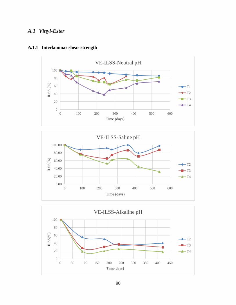
90
A.1 Vinyl-Ester
A.1.1 Interlaminar shear strength
0
20
40
60
80
100
0 100 200 300 400 500 600
ILS
S (
%)
Time (days)
VE-ILSS-Neutral pH
T1
T2
T3
T4
0.00
20.00
40.00
60.00
80.00
100.00
0 100 200 300 400 500 600
ILS
S(%
)
Time (days)
VE-ILSS-Saline pH
T2
T3
T4
0
20
40
60
80
100
0 50 100 150 200 250 300 350 400 450
ILS
S(%
)
Time(days)
VE-ILSS-Alkaline pH
T2
T3
T4

91
A.1.2 Tensile strength
0.00
20.00
40.00
60.00
80.00
100.00
0 20 40 60 80 100 120 140 160
TS
(%
)
Time (days)
VE-TS-Neutral pH
T2
T3
T4
0.00
20.00
40.00
60.00
80.00
100.00
0 50 100 150 200 250
TS
(%
)
Time (days)
VE-TS-Saline pH
T2
T3
T4
0.00
20.00
40.00
60.00
80.00
100.00
0 100 200 300 400 500 600
TS
(%
)
Time (days)
VE-TS-Alkaline pH
T2
T3
T4

92
A.1.3 Flexural strength
0.00
20.00
40.00
60.00
80.00
100.00
0 100 200 300 400 500 600
FS
(%
)
Time (days)
VE-FS-Neutral pH
T2
T3
T4
0.00
20.00
40.00
60.00
80.00
100.00
0 100 200 300 400 500 600
FS
(%
)
Time (days)
VE-FS-Saline pH
T2
T3
T4

93
A.2 Polyester
A.2.1 Interlaminar shear strength
0.00
20.00
40.00
60.00
80.00
100.00
0 100 200 300 400 500 600
ILS
S (
%)
Time (days)
PE-ILSS-Neutral pH
T2
T3
T4
0.00
20.00
40.00
60.00
80.00
100.00
0 100 200 300 400 500 600
ILS
S (
%)
Time (days)
PE-ILSS-Saline pH
T2
T3
T4
0.00
20.00
40.00
60.00
80.00
100.00
0 100 200 300 400 500
ILS
S (
%)
Time (days)
PE-ILSS-Alkaline pH
T2
T3
T4

94
A.2.2 Tensile strength
A.2.3 Flexural strength
0
20
40
60
80
100
120
0 50 100 150 200 250 300 350 400
TS
(%
)
Time (days)
PE-TS-Neutral pH
T2
T3
T4
0.00
20.00
40.00
60.00
80.00
100.00
0 100 200 300 400 500 600
TS
(%
)
Time (days)
PE-TS-Saline pH
T2
T3
T4
0.00
20.00
40.00
60.00
80.00
100.00
0 100 200 300 400 500 600
FS
(%
)
Time (days)
PE-FS-Neutral pH
T2
T3
T4

95
.
0.00
20.00
40.00
60.00
80.00
100.00
0 100 200 300 400 500 600
FS
(%
)
Time (days)
PE-FS-Saline pH
T2
T3
T4

96
APPENDIX B FIELD DATA
The available data for naturally aged data is presented in this Appendix. Under the limitations
presented by the research for this research, the narrow data for field weathering samples resulted
for Vinyl-ester under neutral pH.
#SAMPLE THICKNESS
(in)
YEAR OF
MANUFACTURING
AGE
(years)
AGE
(months)
1 0.212 1993 21 252
2 0.252 1992 22 264
3 0.254 2004 10 120
4 0.26 2002 12 144
5 0.374 2002 12 144
6 0.22 2002 12 144
7 0.126 2005 9 108
8 0.219 2002 12 144
9 0.246 2005 9 108
10 0.375 1995 19 228
11 0.431 2004 10 120
12 0.143 2003 11 132
13 0.308 2009 5 60
14 0.375 2009 5 60
B.1 Flexural data
Sample
# FVF t0
TIME
(months)
Original
strength
Aged
strength
%Origina
l %Aged Notes
1 38.2 0 252
39.29 Missing original str
2 45.4 0 264
55.06 Missing original str
2 web 38.7 0 264
53.48 Missing original str
3 45.2 0 120
54.5 Missing original str
3 web 49.1 0 120 66.1 60.96 100 92.223
3 web/
trans
49.1 0 120
17.65 Missing original str
4 44.4 0 144 59.9 61.83 100 103.22 Post Curing. Data
neglected
4
web/tran
s
40.7 0 144 21.9 22.16 100 101.18 Post Curing. Data
neglected
5 52.7 0 144 51.61 47.37 100 91.784

97
5 web 45.7 0 144 43.69 45.44 100 104.00 Post Curing. Data
neglected
6 43.3 0 144 81.7 40.54 100 49.620
7 47.6 0 108
57.54 Missing original str
8 39.4 0 144 53.86 39.77 100 73.83958
4
9 44.8 0 108 67.5 70.05 100 103.77 Post Curing. Data
neglected
9 web 49.7 0 108 72.2 84.77 100 117.40 Post Curing. Data
neglected
10 37.8 0 228
46.63 Missing original str
10 web 37.9 0 228
47.08 Missing original str
10 web
/trans
37.9 0 228
14.01 Missing original str
11 53.9 0 120 38.2 45.14 100 118.16 Post Curing. Data
neglected
12 sun
side
43.9 0 132 66.82 49.05 100 73.406
12 earth
side
43.9 0 132 66.82 48.02 100 71.864
13 46.3 0 60
55.82 Missing original str
13 trans 46.3 0 60
9.53 Missing original str
14 38.7 0 60
28.27 Missing original str
14 web 39.6 0 60
229.31 Missing original str
14web
/trans
39.6 0 60
14.42 Missing original str
15 43.3
51.27 Missing original str
y = -3.458ln(x) + 104.14
R² = 0.3047
1 10 100 1000 10000
0
20
40
60
80
100
120
TIME (days)
Fle
xura
l S
rt (
% o
f th
e o
rigin
al)
Natural Aging for Flexural streength VE

98
B.2 Tensile strength
Sample # FVF t0 TIME
(months)
Original
strength
Aged
strength
%Original %Aged Notes
1 38.2 0 264 36.11 59.64 100 165 Post Curing. Data
neglected
2 45.4 0 120 37.78 59.18 100 157 Post Curing. Data
neglected
2 web 38.7 0 120 34.15 39.49 100 116 Post Curing. Data
neglected
3 45.2 0 144 53.7 40.48 100 75
3 web 49.1 0 144 53.7 47.75 100 89
4 44.4 0 144 41.7 42.81 100 103 Post Curing. Data
neglected
5 web 45.7 0 144 39.38 35.03 100 89
6 43.3 0 144 63.41 52.69 100 83
7 47.6 0 108 - 65.31 Missing original str
8 39.4 0 144 59.98 48.3 100 81
9 44.8 0 108 54.8 67.84 100 124 Post Curing. Data
neglected
9 web 49.7 0 108 60 72.41 100 121 Post Curing. Data
neglected
10 37.8 0 228 - 36.87 Missing original str
10 web 37.9 0 228 - 33.14 Missing original str
11 53.9 0 120 38.4 40.54 100 106 Post Curing. Data
neglected
12 sun side 43.9 0 132 45.6 36.26 100 80
12 earth
side
43.9 0 132 45.6 34.15 100 75
13 46.3 0 60 - 56.08 Missing original str
13 trans 46.3 0 60 - 4.78 Missing original str
14 38.7 0 60 - 30.45 Missing original str
14 web 39.6 0 60 - 29.35 Missing original str
14web/trans 39.6 0 60 - 38.6 Missing original str

99
B.3 Interlaminar Shear Strength
Sample # FVF t0 TIME
(months)
Original
strength
Aged
strength
%Original %Aged Notes
1 38.2 0 264 - 4237 Missing original str
1 transverse 38.2 0 264 - 1859 Missing original str
2 45.4 0 120 - 3330 Missing original str
2 web 38.7 0 120 - 2615 Missing original str
2 web/trans
- 1946 Missing original str
3 45.2 0 144 8177 5049 100 61.74
3 web 49.1 0 144 8177 5003 100 61.18
3 web/trans 49.1 0 144 - 2829 Missing original str
4 44.4 0 144 5230 4339 100 82.96 *
4 transverse
- 2814 Missing original str
4 web/trans 40.7 0 144 - 2389 Missing original str
5 52.7 0 144 8366 3778 100 45.15
5 web 45.7 0 144 5284 3335 100 63.11
5 web/trans
- 3084 Missing original str
6 43.3 0 108 5509 4172 100 75.73
6 trans
- 2417 Missing original str
7 47.6 0 144 - 5148 Missing original str
7 trans
- 1939 Missing original str
8 39.4 0 108 7310 4338 100 59.34
8 trans
- 2172 Missing original str
9 44.8 0 228 5040 4502 100 89.32 *.
y = -2.52ln(x) + 102.66
R² = 0.5898
1 10 100 1000 10000
0
20
40
60
80
100
120
TIME (days)
Ten
sile
str
ength
(%
of
the
ori
gin
al)
Natural Aging for Tensile str VE

100
9 web 49.7 0 228 4690 4950 100 105.54371 Post Curing. Data
neglected
9 web/ trans
- 2507 Missing original str
10 37.8 0 120 - 4239 Missing original str
10 web 37.9 0 120 - 2638 Missing original str
10 web/trans 37.9 0 120 - 19331 Missing original str
11 53.9 0 132 4287 3906 100 91.11 *
11 trans
- 3118 Missing original str
12 sun side 43.9 0 60 - 4176 Missing original str
12 sun trans
- 4029 Missing original str
12 earth side 43.9 0 60 - 3661 Missing original str
12 earth trans
- 4498 Missing original str
13 46.3 0 60 - 3205 Missing original str
13 transverse 46.3 0 60 - 1409 Missing original str
14 38.7 0 0 - 2551 Missing original str
14 web 39.6 0 0 - 2677 Missing original str
14web/trans 39.6 0 0 - 1736 Missing original str
15 43.3
- 4332 Missing original str
* Post curing could be assumed as the data is out of average and in the rest of strength post curing happened
y = -4.762ln(x) + 100.39
R² = 0.7507
1 10 100 1000 10000
0
20
40
60
80
100
120
TIME (DAYS)
Shea
r S
tr (
% o
f th
e o
rigin
al)
Natural aging for shear str VE

101
APPENDIX C ARRHENIUS PLOTS
As mentioned in Chapter 4, the Arrhenius plots obtained from the previously presented
degradation plots is shown in this Appendix.
C.1 Vinyl-ester Arrhenius plots
C.1.1 Tensile Strength (TS)
y = 264.3e-0.341x
y = 163.46e-0.132x
y = 267.57e-0.065x
10
100
1000
2.9 3 3.1 3.2 3.3 3.4 3.5 3.6
Tim
e to
rea
ch s
elec
ted
FR
P s
tren
gth
val
ue
(day
s)
1/T(x10^3) °K^-1
VE-TS-SALINE PH
90% 80% 70%
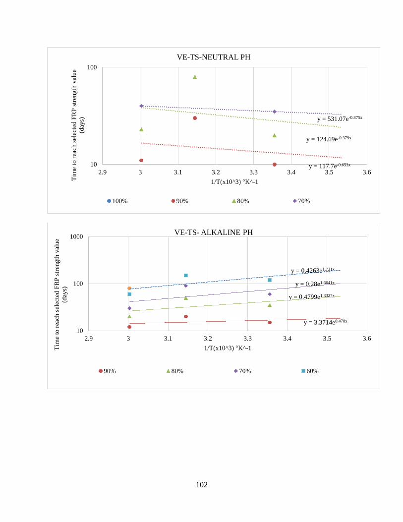
102
y = 117.7e-0.653x
y = 531.07e-0.875x
y = 124.69e-0.379x
10
100
2.9 3 3.1 3.2 3.3 3.4 3.5 3.6
Tim
e to
rea
ch s
elec
ted
FR
P s
tren
gth
val
ue
(day
s)
1/T(x10^3) °K^-1
VE-TS-NEUTRAL PH
100% 90% 80% 70%
y = 3.3714e0.478x
y = 0.4799e1.3327x
y = 0.28e1.6641x
y = 0.4263e1.731x
10
100
1000
2.9 3 3.1 3.2 3.3 3.4 3.5 3.6
Tim
e to
rea
ch s
elec
ted
FR
P s
tren
gth
val
ue
(day
s)
1/T(x10^3) °K^-1
VE-TS- ALKALINE PH
90% 80% 70% 60%

103
C.1.2 Flexural Strength (FS)
y = 11793e-1.813x
y = 447.03e-0.465x
1
10
100
1000
2.9 3 3.1 3.2 3.3 3.4 3.5 3.6Tim
e to
rea
ch s
elec
ted
FR
P s
tren
gth
val
ue
(day
s)
1/T(x10^3) °K^-1
VE-FS-SALINE PH
90% 80% 70%
y = 6E-07e5.5496x
y = 2E-05e4.8059x
10
100
1000
2.9 3 3.1 3.2 3.3 3.4 3.5 3.6
Tim
e to
rea
ch s
elec
ted
FR
P s
tren
gth
val
ue
(day
s)
1/T(x10^3) °K^-1
VE-FS-NEUTRAL PH
90% 80% 70% 60%

104
C.1.3 Interlaminar Shear Strength (ILSS)
y = 2E-05e4.8603x
y = 0.0002e4.3055x
10
100
1000
2.9 3 3.1 3.2 3.3 3.4 3.5 3.6
Tim
e to
rea
ch s
elec
ted
FR
P s
tren
gth
val
ue
(day
s)
1/T(x10^3) °K^-1
VE-ILSS-SALINE PH
90% 80% 70% 60% 50% 40% 30%
y = 5E-05e4.541x
y = 9E-06e5.2267x
y = 4E-06e5.6371x
y = 3E-06e5.9036x
10
100
1000
10000
2.9 3 3.1 3.2 3.3 3.4 3.5 3.6
Tim
e to
rea
ch s
elec
ted
FR
P s
tren
gth
val
ue
(day
s)
1/T(x10^3) °K^-1
VE-ILSS-NEUTRAL PH
90% 80% 70% 60% 50% 40%

105
C.2 Polyester Arrhenius plots
C.2.1 Tensile Strength (TS)
y = 0.0654e1.6925x
y = 0.0995e1.7594x
y = 0.188e1.7028x
y = 0.1599e1.8583x
y = 0.0081e2.9018x
y = 1E-04e4.4105xy = 9E-05e4.5489x
10
100
1000
2.9 3 3.1 3.2 3.3 3.4 3.5 3.6
Tim
e to
rea
ch s
elec
ted
FR
P s
tren
gth
val
ue
(day
s)
1/T(x10^3) °K^-1
VE-ILSS- ALKALINE PH
90% 80% 70% 60% 50% 40% 30% 20%
y = 2671.2e-1.187x
y = 6937e-1.306x
1
10
100
1000
2.9 3 3.1 3.2 3.3 3.4 3.5 3.6Tim
e to
rea
ch s
elec
ted
FR
P s
tren
gth
val
ue
(day
s)
1/T(x10^3) °K^-1
PE-TS-SALINE PH
90% 80% 70%

106
C.2.2 Flexural Strength (FS)
y = 1.4313e0.7911x
y = 1.3866e1.1275x
y = 2.0958e1.2871x
10
100
1000
2.9 3 3.1 3.2 3.3 3.4 3.5 3.6Tim
e to
rea
ch s
elec
ted
FR
P s
tren
gth
val
ue
(day
s)
1/T(x10^3) °K^-1
PE-TS-NEUTRAL PH
100% 90% 80% 70% 60% 50%
y = 71.557e0.0619x
1
10
100
1000
2.9 3 3.1 3.2 3.3 3.4 3.5 3.6Tim
e to
rea
ch s
elec
ted
FR
P s
tren
gth
val
ue
(day
s)
1/T(x10^3) °K^-1
PE-FS-SALINE PH
90% 80%

107
C.2.3 Interlaminar Shear Strength (ILSS)
y = 439.6e-0.631x
y = 9E-06e5.4584x
10
100
1000
10000
2.9 3 3.1 3.2 3.3 3.4 3.5 3.6
Tim
e to
rea
ch s
elec
ted
FR
P s
tren
gth
val
ue
(day
s)
1/T(x10^3) °K^-1
PE-FS-NEUTRAL PH
90% 80% 70%
y = 0.0289e2.2186x
y = 0.0023e3.177x
y = 0.0399e2.3754x
10
100
2.9 3 3.1 3.2 3.3 3.4 3.5 3.6
Tim
e to
rea
ch s
elec
ted
FR
P s
tren
gth
val
ue
(day
s)
1/T(x10^3) °K^-1
PE-ILSS-SALINE PH
90% 80% 70% 60% 50% 40%

108
y = 1.2343e0.9892x
y = 13.052e0.3228x
y = 19.847e0.221x
y = 30.345e0.1243x
y = 0.1838e1.9752x
10
100
2.9 3 3.1 3.2 3.3 3.4 3.5 3.6
Tim
e to
rea
ch s
elec
ted
FR
P s
tren
gth
val
ue
(day
s)
1/T(x10^3) °K^-1
PE-ILSS-NEUTRAL PH
90% 80% 70% 60% 50% 40%
y = 0.3261e1.1424x
y = 1.496e0.8601x
y = 2.2886e0.846x
y = 1.8982e0.9982x
y = 2.6121e0.9753x
y = 1.679e1.18xy = 9.6424e0.7438x
10
100
2.9 3 3.1 3.2 3.3 3.4 3.5 3.6
Tim
e to
rea
ch s
elec
ted
FR
P s
tren
gth
val
ue
(day
s)
1/T(x10^3) °K^-1
PE-ILSS- ALKALINE PH
90% 80% 70% 60% 50% 40% 30% 20%

109
APPENDIX D TIME SHIFT FACTOR-TEMPERATURE
RELATIONSHIPS
To be able to get time shift factors to different temperatures and be able to extrapolate the
TSF related to different temperatures the relationship between TSF and temperature was obtained
and presented as can be seen in the figures below.
y = 0.055e0.7733x
R² = 0.0409y = 0.3068e0.3177x
R² = 0.0482
y = 5E+09e-6.644x
R² = 1
0
2
4
6
8
10
12
2.95 3 3.05 3.1 3.15 3.2 3.25 3.3 3.35 3.4
TS
F
1/Temperature(°K-1)
TSF vs T° VE-TS
Neutral pH Lower pH (4-6)Alkaline (pH=13) Expon. (Lower pH (4-6))Expon. (Alkaline (pH=13))

110
y = 24.987e-0.964x
R² = 0.9562y = 0.0181e1.2449x
R² = 0.2721
0
0.2
0.4
0.6
0.8
1
1.2
1.4
1.6
2.95 3 3.05 3.1 3.15 3.2 3.25 3.3 3.35 3.4
TS
F
1/Temperature(°K-1)
TSF vs T° PE-TS
Neutral pH Lower pH (4-6)
Expon. (Lower pH (4-6))
y = -1.8898x + 7.2948
R² = 0.9164y = -5.3045x + 18.537
R² = 0.7305
0
0.5
1
1.5
2
2.5
3
3.5
2.95 3 3.05 3.1 3.15 3.2 3.25 3.3 3.35 3.4
TS
F
1/Temperature(°K-1)
TSF vs T° EX-TS
Lower pH (4-6) Alkaline (pH=13)
Linear (Lower pH (4-6)) Linear (Alkaline (pH=13))

111
y = 4E+07e-5.224x
R² = 0.9806y = 0.0323e1.0634x
R² = 0.2893
0
1
2
3
4
5
6
7
2.95 3 3.05 3.1 3.15 3.2 3.25 3.3 3.35 3.4
TS
F
1/Temperature(°K-1)
TSF vs T° VE-FS
Neutral pH Lower pH (4-6)
Expon. (Neutral pH) Expon. (Lower pH (4-6))
y = 0.1251e0.6308x
R² = 0.6465y = -0.2227x + 2.0776
R² = 0.003
0
0.5
1
1.5
2
2.5
2.95 3 3.05 3.1 3.15 3.2 3.25 3.3 3.35 3.4
TS
F
1/Temperature(°K-1)
TSF vs T° PE-FS
Neutral pH Lower pH (4-6)
Expon. (Neutral pH) Linear (Lower pH (4-6))
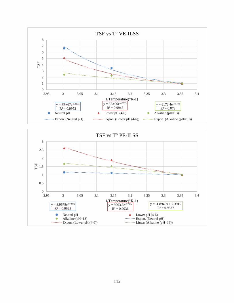
112
y = 8E+07e-5.413x
R² = 0.9953
y = 5E+06e-4.597x
R² = 0.9943y = 6173.4e-2.578x
R² = 0.879
0
1
2
3
4
5
6
7
8
2.95 3 3.05 3.1 3.15 3.2 3.25 3.3 3.35 3.4
TS
F
1/Temperature(°K-1)
TSF vs T° VE-ILSS
Neutral pH Lower pH (4-6) Alkaline (pH=13)
Expon. (Neutral pH) Expon. (Lower pH (4-6)) Expon. (Alkaline (pH=13))
y = 3.9678e-0.409x
R² = 0.9623y = 9903.6e-2.736x
R² = 0.9936
y = -1.8945x + 7.3915
R² = 0.9537
0
0.5
1
1.5
2
2.5
3
2.95 3 3.05 3.1 3.15 3.2 3.25 3.3 3.35 3.4
TS
F
1/Temperature(°K-1)
TSF vs T° PE-ILSS
Neutral pH Lower pH (4-6)Alkaline (pH=13) Expon. (Neutral pH)Expon. (Lower pH (4-6)) Linear (Alkaline (pH=13))

113
APPENDIX E ACCELERATED SHIFTED DATA FOR LONG
TERM DEGRADATION TRENDS
After obtaining the Time Shift Factors for the different cases presented in Chapter 5, a longer-
term degradation curves are extrapolated for the acceleratedly aged samples and presented in this
Appendix.
y = -3.088ln(x) + 96.623
R² = 0.6682
y = -2.398ln(x) + 89.67
R² = 0.6544
y = -5.183ln(x) + 95.696
R² = 0.9099
0
20
40
60
80
100
120
0 500 1000 1500 2000 2500 3000 3500 4000
FS
(%)
Time (days)
VE-FS-Shifted data-Corrected
p3 p2 p5
Log. (p3) Log. (p2) Log. (p5)

114
y = -3.024ln(x) + 91.418
R² = 0.5147
y = -2.411ln(x) + 98.388
R² = 0.7599
y = -10.99ln(x) + 95.82
R² = 0.79490.00
20.00
40.00
60.00
80.00
100.00
120.00
0 100 200 300 400 500 600 700
FS
(%
)
Time (days)
PE-FS -Shifted data-Corrected
P3 P2 P5
Log. (P3) Log. (P2) Log. (P5)
y = -3.075ln(x) + 93.477
R² = 0.4599
y = -3.218ln(x) + 95.007
R² = 0.453
y = -15.24ln(x) + 122.38
R² = 0.89780
20
40
60
80
100
120
0 500 1000 1500 2000 2500 3000 3500 4000
ILS
S (
%)
Time (days)
VE-ILSS-Shifted data-Corrected
P3 P2 P5
Log. (P3) Log. (P2) Log. (P5)

115
y = -6.992ln(x) + 83.9
R² = 0.654
y = -5.021ln(x) + 95.084
R² = 0.4324
y = -11.4ln(x) + 89.288
R² = 0.9389
0
20
40
60
80
100
120
0 200 400 600 800 1000 1200 1400 1600
ILS
S (
%)
Time (days)
PE-ILSS-Shifted data-Corrected
p3 p2 p5
Log. (p3) Log. (p2) Log. (p5)
y = -3.485ln(x) + 87.566
R² = 0.6805
y = -5.243ln(x) + 94.317
R² = 0.7358
y = -4.292ln(x) + 101.69
R² = 0.8403
y = -5.435ln(x) + 93.573
R² = 0.61420
20
40
60
80
100
120
0 100 200 300 400 500 600 700 800 900 1000
TS
(%)
Time (days)
VE-TS-Shifted data-Corrected
p3 p2 p4 p5
Log. (p3 ) Log. (p2 ) Log. (p4) Log. (p5)
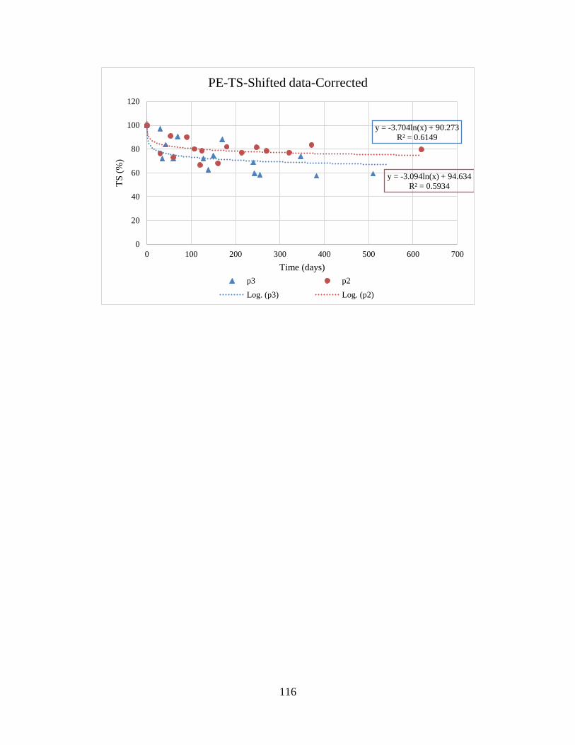
116
y = -3.704ln(x) + 90.273
R² = 0.6149
y = -3.094ln(x) + 94.634
R² = 0.5934
0
20
40
60
80
100
120
0 100 200 300 400 500 600 700
TS
(%
)
Time (days)
PE-TS-Shifted data-Corrected
p3 p2
Log. (p3) Log. (p2)
117
APPENDIX F .DETERMINATION OF STRENGTH
REDUCTION FACTORS “φ”
Ongoing research at West Virginia University (WVU) indicates the process used to determine
the strength reduction factors Phi “φ” in design codes, which is based on reliability indices of
probabilistic approaches. Determining these factors involves the adoption of the “probability of
failure” criterion under the different circumstances.
The “probability of failure” criterion suggests that in practice, the occurrence and
consequences of accident can be associated with certain risk level, which is stablished in the design
codes and standards. A zero-risk level is unlikely to be reached, thus a residual risk level needs to
be determined by a combination of cost, safety and public reaction resulting from failures (CEN,
2004).
In previous codes, the deterministic methods were used to compute the different factors of
safety which often resulted in non-uniform probability of failures.
The structural reliability method attempts to select a 𝜑 factor for the structural design strength
“𝑅” that will provide an appropriate and uniform probability of failure when the structural element
is subjected to the 𝑄 load effect, as can be seen in Equation F-1.
𝜑 ∙ 𝑅 ≥ 𝛾 ∙ 𝑄 (F-1)
The modification factor,𝛾, has already been tabulated in most of the Load and Resistance
Factor Design (LRFD) codes, so the main interest falls back onto obtaining the 𝜑 factor for
structural components made of materials different from the conventional, as FRP composites.
The method to determine the 𝜑 factors is as follows:

118
1. Select the reliability index β. Most of the codes in the United States and Canada
have adopted an acceptable reliability index of 3.5 or higher. This index is a
theoretical value for probability of failure of approximately 1 in 5,000.
2. Develop probability density functions of the material properties used to compute
“R” using the data from lab tests or the given by the manufacturer. Instead of
developing the probability density functions for each design parameters, mean
values, bias factors and standard deviation are used.
3. Select the common design situation (span length, loading, environment, member
size, etc.) in which 𝜑 factor will be used. Some parameters are assumed to be
constant, whereas others could be variable in the probability density functions. For
example, the span length of the structure is assumed to be a precise parameter
whereas the yield strength (Fy) or a distributed load (w) are assumed to be variable.
4. Write the reduced limit state design equation in terms of the variables. Compute
mean values and standard deviations for the variables. For example:
𝐺(𝑤, 𝐹𝑦) = 𝜑 ∙ 𝑅 − 𝛾 ∙ 𝑄 (F-2)
5. Select a trial value for 𝜑. 1.0 is a good reference point to be able to compute a
nominal value of β, leaving the reduced limit state equation in terms of the
variables. Continuing with the previous example, where a1 and a2 are computed
constants:
𝐺(𝑤, 𝐹𝑦) = 𝑎1 ∙ 𝐹𝑦 − 𝑎2 ∙ 𝑤 (F-3)

119
6. Having obtained the mean value (μ) and standard deviation (σ) of the different
parameters, compute the nominal β and compare it to the target value. In simplistic
form, it can be computed as:
𝛽 =
𝑎1 ∙ μ(𝐹𝑦) − 𝑎2 ∙ μ(𝑤)
√𝑎1 ∙ σ(𝐹𝑦)2 − 𝑎2 ∙ σ(𝑤)2
(F-4)
7. Adjust 𝜑 doing an iterative process of steps 5 and 6 until obtaining a 𝛽 close to the
objective.
8. For the different cases repeat steps 3 to 7 and obtain the corresponding values of 𝜑
for each one.
9. Select a conservative value of 𝜑.
The obtained strength reduction “𝜑” factors account for the statistical variability of the
strength values along the designed service life, or 75 to 100 years. The available values for the 𝜑
factors are considered to be conservative by many experts. By following the process presented in
this thesis, an overall view of the different durability researches is given in order to obtain more
rational values for the strength reduction factors for design purposes. To have the most accurate
approximation to the optimal phi factors the maximum available data is needed, either of
accelerated data or naturally aged samples.