Durability of Adhesive Joints Subjected To - Virginia Tech

1

Durability of Adhesive Joints Subjected

To Environmental Stress

by

Emmett P. O’Brien

Dissertation for Doctor of Philosophy

in

Chemical Engineering

Virginia Polytechnic Institute and State University

Blacksburg, Virginia 24060

Committee Chair: Thomas C. Ward

Committee Members:

Dr. Richey Davis

Dr. David Dillard

Dr. Eva Marand

Dr. Ravi Saraf

August 28, 2003

Key Words: polymer, adhesion, environmental degradation, epoxy, water, interface, durability, diffusion,

shaft-loaded blister test, sub-critical crack growth, electrochemical impedance spectroscopy (EIS),

dielectric spectroscopy, ink

2

Title: Durability of Adhesive Joints Subjected to Environmental Stress

Author: Emmett P. O’Brien

Abstract

Environmental stresses arising from temperature and moisture changes, and/or other aggressive

fluid ingressions can degrade the mechanical properties of the adhesive, as well as the integrity

of an adhesive interface with a substrate. Therefore such disruptions can significantly reduce the

lifetime and durability of an adhesive joint.1-4 In this research, the durability of certain epoxy

adhesive joints and coatings were characterized using a fracture mechanics approach and also by

constant frequency impedance spectroscopy.

The shaft-loaded blister test (SLBT) was utilized to measure the strain energy release rate

(G) or adhesive fracture energy of a pressure sensitive adhesive tape. In this study, support for

the value of the SLBT fracture mechanics approach was obtained. The SLBT was then used to

investigate the effects of relative humidity on a model epoxy bonded to silicon oxide. Lastly, the

effects of water and temperature on the adhesion of a commercial filled epoxy bonded to silicon

oxide was characterized and interpreted.

A novel impedance sensor for investigating adhesion was developed in a collaborative

effort between Virginia Tech and Hewlett-Packard. Utilizing the technique of constant frequency

impedance spectroscopy, the distribution and transport of fluids at the interface of adhesive joints

was measured. A broad spectrum of adhesives was tested. In addition, the effects of hygroscopic

cycling on the durability of adhesive coatings were measured for the commercial filled epoxy

using the device. Lastly, recommended modifications of the experimental set-up with the new

sensor are proposed to improve the technique.

iii

Acknowledgements

I would like to sincerely thank the following people. You have made the time at Virginia Tech

well spent.

Dr. Ward, thank you for all your advice and support throughout the years (personal and

professional) and giving me the opportunity to obtain a Ph.D. Thank you for giving our group the

intellectual freedom and resources to pursue our own scientific interests. Thank you opportunity

to attend numerous conferences, visit interesting places, and meet many important people in

industry.

My committee members: Dr. Richey Davis, Dr. David A. Dillard, Dr. Eva Marand and Dr. Ravi

Saraf for their tough questions, valuable suggestions and even more valuable time.

I would like to particularly thank David A. Dillard for teaching me about adhesives and

adhesives research from a both a practical and fundamental standpoint. Thank you for guiding

me through fracture mechanics and giving me the chance to earn a living at breaking things.

Thank you also for introducing me to many people in the adhesives industry and for the

opportunity to network in places like Yosemite, CA.

Thanks to all my friends and professional colleagues, especially Sandra Case who graduated

right before me and showed me the way. Thanks to Amy Eichstadt for keeping my shoes. Thank

you Rob Jensen for mentoring me in the embryonic stage of graduate school. Thanks to Dave

Porter for teaching me to rig stuff up. Thanks to Taigyoo Park for introducing me to the SLBT.

Corey Reed and Jeremy Lizotte for several championships. Thanks to everyone else: Kermit

Kwan, Jennifer Robertson, Ojin Kwan, Chitra Subraminiam, Jaime Kalista, Hailing Yang,

Kalpana Viswanathan, Ron Defelice, Mitch and Brenda Jackson, Mike Bortner, Eric Scribben,

Scott Trenor, Jeremy Lizotte, Lee Williams, The Hunsuckers, Matt O’Sickey, Dave Godshall,

Chris Robertson, Martha McCaann, Bradford Carmen, Doug Crowson, Anders DiBiccari, Holly

Grammer, and Derek and Kelly.

iv

I would like to thank every one in the Hewlett-Packard project including Dr. John G. Dillard, Dr.

James. E. McGrath, Sumitra Subraminian, Johnny Yu, Sankar, Hitendra Singh, Shu Guo, David

Xu, and Zuo Sun. I would like to thank the folks at Hewlett-Packard: Thank you Paul Reboa and

Thomas Lindner for great project management and the numerous hefe-weizens. Thank you

Marshall Field, Dan Pullen, and David Markel for design and production of the impedance

sensors. Thank you Jim McKinnel for the numerous tutorials on electrical engineering. Thanks to

Josh Smith for his big brain. Despite what people say, you are not really a jackass. Thanks to

Brad Benson. Thanks to Ellen Chappell.

Thanks to the Center for Adhesive and Sealant Science: Dr James P. Wightman, Tammy Jo

Hiner, and Linda Haney. Thanks to the Adhesive and Sealant Council and all the great people

that I have met through the ASC. Great folks like Malinda Armstrong, Wendy Yanis, Dave

Jackson, Rick Barry, Robert Lefelar, Jim Sorg, Kay Peters, Norman Pfeifer, Darrel Bryant, Rick

Jihnston, Dwight Lynch The guys from Franklin International Adhesives: Mark Vrana, Larry

Owen, Larry Gwin, Matt McGreery, Chusk Shuster, Dale and Evan Williams. The folks at

Adhesives Research Incorporated: Ranjit Malik and Brian Harkins.

Thank you, Professor J. E. “Big Jim” McGrath for all your help, friendship, and nights at the

Karaoke bar. Thanks to Professors Judy Riffle and Alan Esker. Thanks to the friends and folks at

TA Instruments: Gary Mann and Steve Aubuchon. Thanks to the following SURPs: Kevin

Doyle, Stefan Adreev, and Wes. Thank you Michael Vick and Corey Moore. Thanks to all my

undergrad friends: Ray and Tammy, Kirrukk, Kollman, Hinett, Rich, Castello, Sujan, Maharshi,

Guarav, Raindeer, Ceasar, Cindy, and Laura. Thanks to Millie Ryan, Laurie Good, and Esther

Brann who were always so nice and willing to lend an ear or a cup of coffee. Thanks to Frank

Cromer for hanging out and letting me use the sputter coater. Thanks to Jim Coulter for his

electrical engineering tutorials and to Travis for helping with computer woes. Thanks to Al

Shultz, Dr. Garth Wilkes, Diane Cannaday, Dr. William Conger, and Diane Patty. Thanks to the

Physics Machine Shop rednecks: Scott, John, Melvin, Melvin’s cousin and even Fred (O.D.B.).

Thanks to Jane for keeping our lab tidy. Thanks to the boys in Boulder, Co. and Aaron

v

Campbell. Thanks to people in Dart League, early morning tailgaters, and NASCAR people.

Thanks to the late Francis VanDamme.

I have saved thanking the most important people in my life for last. I would like to thank my

mom, Esperanza R. O’Brien for all her love and support over the years. Mom, I finally got a real

job. Thank you, my wife, Kristen W. O’Brien for your love, good times, and improving my

writing skills. Thank you to all of Kristen’s family for being such great people and raising such a

special woman.

Good luck to all the new graduate students, you will need it.

vi

Table of Contents

DURABILITY OF ADHESIVE JOINTS SUBJECTED TO ENVIRONMENTAL STRESS ..............................1

1 INTRODUCTION..............................................................................................................................................1

2 BACKGROUND ON ENVIRONMENTAL DEGRADATION OF ADHESIVE JOINTS AND

COATINGS..................................................................................................................................................................3

2.1 FACTORS THAT INFLUENCE WATER TRANSPORT AND SUBSEQUENT ADHESION LOSS ................................3

2.2 GENERAL TRENDS REGARDING LOSS OF ADHESION ...................................................................................4

2.3 HYPOTHESIS AND MECHANISM FOR LOSS OF ADHESION BY WATER...........................................................5

2.3.1 Water Accumulation at the Interface .....................................................................................................5

2.3.2 The Heterogeneous Nature of Adhesive Bond: Water Transport and Accumulation.............................7

2.3.3 Osmotic Forces and Lateral Growth by Continued Condensation and Blistering ................................7

2.3.4 Physisorption of Water at the Interface .................................................................................................8

2.4 METHODS TO INCREASE THE LIFETIME OF ADHESIVE BONDS .....................................................................8

2.5 DIFFUSION IN POLYMERS AND ADHESIVE JOINTS......................................................................................10

2.5.1 Fickian Diffusion .................................................................................................................................10

2.5.2 Non-Fickian Diffusion .........................................................................................................................12

2.5.3 Interfacial Diffusion and Diffusion in Adhesive Joints ........................................................................13

2.5.4 Diffusion in Epoxies.............................................................................................................................15

3 ADHESIVE STUDIES USING THE SHAFT-LOADED BLISTER TEST................................................17

3.1 INTRODUCTION..........................................................................................................................................17

3.2 STRAIN ENERGY RELEASE RATES OF A PRESSURE SENSITIVE ADHESIVE TAPE MEASURED BY THE SHAFT-

LOADED BLISTER TEST............................................................................................................................................18

3.2.1 Abstract................................................................................................................................................18

3.2.2 Introduction to Adhesive Testing of Thin Coatings..............................................................................19

3.2.3 Shaft-Loaded Blister Test Theory ........................................................................................................24

3.2.4 Experimental........................................................................................................................................28

vii

3.2.5 Results and Discussion ........................................................................................................................29

3.2.6 Effects of Fluids at the Interface..........................................................................................................38

3.2.7 Conclusions..........................................................................................................................................40

3.2.8 Appendix: Experimental compliance calibration.................................................................................41

3.2.9 Figures.................................................................................................................................................46

3.3 MOISTURE DEGRADATION OF EPOXY ADHESIVE BONDS MEASURED BY THE SHAFT-LOADED BLISTER

TEST 61

3.3.1 Abstract................................................................................................................................................61

3.3.2 Introduction .........................................................................................................................................61

3.3.3 Experimental........................................................................................................................................63


3.3.5 Conclusion ...........................................................................................................................................67

3.3.6 Figures.................................................................................................................................................68

3.4 ENVIRONMENTAL STUDIES OF ADHESIVE BONDS USING THE SUB-CRITICAL SHAFT-LOADED BLISTER

TEST 71

3.4.1 Abstract................................................................................................................................................71

3.4.2 Introduction .........................................................................................................................................71

3.4.3 Experimental........................................................................................................................................76


3.4.5 Summary ..............................................................................................................................................88

3.4.6 Figures.................................................................................................................................................90

3.4.7 Appendix: Measuring Diffusion Coefficients .......................................................................................99

4 INVESTIGATION OF THE DURABILITY OF ADHESIVE JOINTS AND COATINGS USING

CONSTANT FREQUENCY IMPEDANCE SPECTROSCOPY ........................................................................101

4.1 INTRODUCTION........................................................................................................................................101

4.2 BACKGROUND ON IMPEDANCE SPECTROSCOPY.......................................................................................103

4.2.1 Constant Frequency Impedance Measurements ................................................................................104

4.2.2 The Relationship between Capacitance and Fluid Concentration.....................................................105

viii

4.2.3 Estimating the Area of Debonding.....................................................................................................108

4.2.4 Figures...............................................................................................................................................110

4.3 A NOVEL IMPEDANCE SENSOR DESIGN FOR MEASURING THE DISTRIBUTION AND TRANSPORT OF FLUIDS

IN ADHESIVE JOINTS..............................................................................................................................................111

4.3.1 Abstract..............................................................................................................................................111

4.3.2 Introduction .......................................................................................................................................111

4.3.3 Experimental......................................................................................................................................113

4.3.4 Results and Discussion ......................................................................................................................116

4.3.5 Summary ............................................................................................................................................117

4.3.6 Figures...............................................................................................................................................119

4.4 DIFFUSION OF WATER AND SUBSEQUENT DEBONDING OF A PSA TAPE ..................................................125

4.4.1 Abstract..............................................................................................................................................125

4.4.2 Materials and Experimental ..............................................................................................................125

4.4.3 Results................................................................................................................................................125

4.4.4 Conclusion .........................................................................................................................................126

4.4.5 Figures...............................................................................................................................................127

4.5 INTERFACIAL DIFFUSION OF AGGRESSIVE FLUIDS INTO EPOXY ADHESIVE JOINTS AND COATINGS

MEASURED BY CONSTANT FREQUENCY IMPEDANCE SPECTROSCOPY ...................................................................128

4.5.1 Abstract..............................................................................................................................................128

4.5.2 Research Objectives...........................................................................................................................128

4.5.3 Experimental......................................................................................................................................129


4.5.5 Conclusions........................................................................................................................................137

4.5.6 Figures...............................................................................................................................................139

4.6 MOISTURE DIFFUSION FROM THE EDGE IN BONDED UV CURABLE PRESSURE SENSITIVE ADHESIVES

MEASURED BY CONSTANT FREQUENCY IMPEDANCE SPECTROSCOPY ...................................................................146

4.6.1 Abstract..............................................................................................................................................146

4.6.2 Experimental......................................................................................................................................146

ix


4.6.4 Conclusions........................................................................................................................................152

4.6.5 Figures...............................................................................................................................................153

4.7 DURABILITY OF ADHESIVE COATINGS SUBJECTED TO HYGROSCOPIC CYCLING MEASURED BY CONSTANT

FREQUENCY IMPEDANCE SPECTROSCOPY..............................................................................................................160

4.7.1 Abstract..............................................................................................................................................160

4.7.2 Introduction .......................................................................................................................................161

4.7.3 Experimental......................................................................................................................................165


4.7.5 Summary ............................................................................................................................................182

4.7.6 Figures...............................................................................................................................................184

4.8 RECOMMENDATIONS AND MODIFICATIONS FOR CONSTANT FREQUENCY INTERFACIAL IMPEDANCE

SPECTROSCOPY......................................................................................................................................................197

4.8.1 Abstract..............................................................................................................................................197

4.8.2 Sources of Signal Noise .....................................................................................................................197

4.8.3 Recommended Modifications .............................................................................................................197

5 CONCLUDING REMARKS.........................................................................................................................200

6 REFERENCES: .............................................................................................................................................201

x

Table of Figures

FIGURE 3-1 SCHEMATIC OF THE PULL-OFF TEST ...........................................................................................................46

FIGURE 3-2 SCHEMATIC OF THE SHAFT-LOADED BLISTER TEST....................................................................................46

FIGURE 3-3 STRESS-STRAIN CURVE FOR KAPTON® PSA..............................................................................................47

FIGURE 3-4 SCHEMATIC OF THE EXPERIMENTAL SET-UP OF THE SHAFT LOADED BLISTER TEST ....................................48

FIGURE 3-5 SCHEMATIC OF VIEW OF BLISTER RADIUS PROPAGATION ..........................................................................49

FIGURE 3-6 LOAD (P) VS. CENTRAL SHAFT DISPLACEMENT (W0) FOR N = 1, 2 AND 4.....................................................50

FIGURE 3-7 DEBONDING RADIUS (A) VS. CENTRAL SHAFT DISPLACEMENT (W0) FOR N = 1, 2 AND 4 ..............................51

FIGURE 3-8 SCHEMATIC OF THE ACTUAL BLISTER PROFILE...........................................................................................52

FIGURE 3-9 LOADING AND UNLOADING CYCLES FOR KAPTON® PSA TAPE BONDED TO POLISHED ALUMINUM. THE

LOADING PORTION OF THE CURVE IS SHOWN IN FILLED SYMBOLS AND THE UNLOADING PORTION IS SHOWN IN

UNFILLED SYMBOLS. ...........................................................................................................................................53

FIGURE 3-10 PLOT OF THE FINAL LOAD PMAX OF EACH CYCLE VS. W0 FOR KAPTON® PSA TAPE BONDED TO POLISHED

ALUMINUM..........................................................................................................................................................54

FIGURE 3-11 PLOT OF EFFECTIVE MEMBRANE STRESS AS A FUNCTION OF CRACK LENGTH (A) AND R............................55

FIGURE 3-12 PLOTS OF PREDICTED SCALING LAWS BASED ON LOAD, HYBRID, AND DISPLACEMENT EQUATIONS..........56

FIGURE 3-13 LOAD (P) VS. CENTRAL SHAFT DISPLACEMENT (W0), AND CRACK LENGTH (A) VS. CENTRAL SHAFT

DISPLACEMENT CURVES (W0), FOR KAPTON® PSA TAPE BONDED TO TEFLON (N = 1).........................................57

FIGURE 3-14 SCHEMATIC OF THE EXPERIMENTAL SET-UP USED TO MAKE IN-SITU MEASURE OF LIQUID INFLUENCE THE

STRAIN ENERGY RELEASE RATE ..........................................................................................................................58

FIGURE 3-15 LOAD (P) VS. CENTRAL SHAFT DISPLACEMENT (W0) FOR VARIOUS CONCENTRATIONS OF METHANOL IN

WATER (0, 40, 60, 80, 100 WT. %).......................................................................................................................59

FIGURE 3-16 LINEARIZED PLOT OF EQUATION 7, P A2 VS. W03 FOR N = 1(□), 2 (О), AND 4 (◊) ........................................60

FIGURE 3-17.SCHEMATIC OF THE SHAFT-LOADED BLISTER TEST ..................................................................................68

FIGURE 3-18 SCHEMATIC OF SHAFT-LOADED BLISTER TEST SPECIMEN.........................................................................68

FIGURE 3-19 SUCCESSIVE LOAD AS A FUNCTION OF CENTRAL SHAFT DISPLACEMENT CURVES FOR 98% RELATIVE

HUMIDITY. THE FILLED IN SYMBOLS ARE THE LOADING CURVES AND THE UNFILLED SYMBOLS ARE THE

UNLOADING CURVES. ..........................................................................................................................................69

xi

FIGURE 3-20. LOAD VS. BLISTER RADIUS FOR 98% RELATIVE HUMIDITY......................................................................70

FIGURE 3-21. SUMMARY OF STRAIN ENERGY RELEASE RATES G (J/M2) VS. RELATIVE HUMIDITY FOR CRITICAL SLBT 70

FIGURE 3-22. SCHEMATIC OF V-G CURVE ILLUSTRATING THREE REGION OF CRACK GROWTH ......................................90

FIGURE 3-23. SCHEMATIC OF TYPICAL BEHAVIOR AS THE CHEMICAL ACTIVITY CHANGES 121.......................................90

FIGURE 3-24 SCHEMATIC OF THE FLUID RESERVOIR FORMED BETWEEN THE ADHESIVE MEMBRANE AND SUBSTRATE..91

FIGURE 3-25 SCHEMATIC OF THE SUB-CRITICAL SHAFT-LOADED BLISTER TEST SPECIMEN. ..........................................91

FIGURE 3-26 PHOTOGRAPH OF L4 ADHESIVE BLISTER SPECIMEN..................................................................................92

FIGURE 3-27 PHOTOGRAPH OF SUB-CRITICAL SHAFT-LOADED BLISTER TEST SPECIMENS IN OVEN ENVIRONMENT. ......93

FIGURE 3-28 SLBT CRACK VELOCITY (M/S) AS A FUNCTION OF CRACK DRIVING ENERGY, G, (J/M2) AND RELATIVE

HUMIDITY (25°C). THE ADHESIVE IS THE MODEL EPOXY.....................................................................................94

FIGURE 3-29 THE CRACK VELOCITY OF REGION II AS A FUNCTION OF RELATIVE HUMIDITY (25°C). THE ADHESIVE IS

THE MODEL EPOXY..............................................................................................................................................94

FIGURE 3-30 SLBT CRACK VELOCITY (M/S) AS A FUNCTION OF CRACK DRIVING ENERGY, G, (J/M2) AND TEMPERATURE.

THE ENVIRONMENT IS WATER AND THE ADHESIVE IS THE L4 EPOXY...................................................................95

FIGURE 3-31 ARRHENIUS PLOT OF THE L4 ADHESIVE PLATEAU VELOCITY EXPOSED TO WATER AT 60, 70, AND 80°C..96

FIGURE 3-32 ARRHENIUS PLOT OF THE L4 ADHESIVE THRESHOLD VALUE OF G EXPOSED TO WATER AT 60, 70, AND

80°C. ..................................................................................................................................................................96

FIGURE 3-33 THE NORMALIZED PERCENT MASS UPTAKE AS A FUNCTION OF THE SQUARE ROOT OF TIME (SECONDS)

NORMALIZED BY THE SAMPLE THICKNESS FOR EACH TEMPERATURE. THE ADHESIVE IS THE L4 EPOXY. .............97

FIGURE 3-34 THE PERCENT MASS UPTAKE AS A FUNCTION OF THE SQUARE ROOT OF TIME (SECONDS) NORMALIZED BY

THE SAMPLE THICKNESS AND FOR EACH TEMPERATURE. THE ADHESIVE IS THE L4 EPOXY. ................................98

FIGURE 3-35 ARRHENIUS PLOT OF THE TEMPERATURE DEPENDENCE OF THE DIFFUSION COEFFICIENT OF WATER IN THE

L4 EPOXY............................................................................................................................................................98

FIGURE 4-1. SCHEMATIC OF THE EXPECTED CAPACITANCE AS A FUNCTION OF EXPOSURE TIME OBTAINED FROM

SINGLE-FREQUENCY IMPEDANCE SPECTROSCOPY. ............................................................................................110

FIGURE 4-2. SCHEMATIC OF THE TIME TO FAILURE DETERMINED GRAPHICALLY FROM THE RESISTANCE AS A FUNCTION

OF TIME OBTAINED FROM SINGLE-FREQUENCY IMPEDANCE SPECTROSCOPY. ....................................................110

xii

FIGURE 4-3 SCHEMATIC (NOT SHOWN TO SCALE) OF THE IIS SENSOR. THE CONTACT PADS ARE LABELED 1 THROUGH

10. ....................................................................................................................................................................119

FIGURE 4-4 PHOTOGRAPH OF THE IIS SENSOR. ...........................................................................................................120

FIGURE 4-5 SCHEMATIC OF THE EXPERIMENTAL SET-UP OF THE SENSOR AND ENVIRONMENTAL CHAMBER. THE PATH

OF DIFFUSION IS SHOWN WITH THE ARROWS......................................................................................................121

FIGURE 4-6 SCHEMATIC OF THE SIDE-VIEW OF THE BONDED PSA TAPE ILLUSTRATING THE PATH OF DIFFUSION OF

ACETONE...........................................................................................................................................................122

FIGURE 4-7 INITIAL REGION (UP TO TWO HOURS) OF THE NORMALIZED CAPACITANCE AS A FUNCTION OF EXPOSURE

TIME (HOURS) FOR DIFFERENT VALUES OF X......................................................................................................123

FIGURE 4-8 THE CONCENTRATION PROFILE OBTAINED FROM IIS SENSOR...................................................................124

FIGURE 4-9. CAPACITANCE AS A FUNCTION OF EXPOSURE TIME FOR THE QUILL PRESSURE SENSITIVE ADHESIVE TAPE IN

WATER. .............................................................................................................................................................127

FIGURE 4-10 SCHEMATIC OF ADHESIVE SANDWICH SPECIMEN....................................................................................139

FIGURE 4-11 SCHEMATIC OF THE ADHESIVE SANDWICH SPECIMEN WITH GLASS SHIM. ...............................................139

FIGURE 4-12 THE CAPACITANCE AS A FUNCTION OF EXPOSURE TIME (DAYS) FOR THE L4 ADHESIVE SANDWICH

SPECIMENS TYPE 1 SAMPLE 1 EXPOSED TO 0.1 M NAOH..................................................................................140


SPECIMENS TYPE 1 SAMPLE 2 EXPOSED TO 0.1 M NAOH..................................................................................140

FIGURE 4-14 NORMALIZED CONCENTRATION (C*) AS A FUNCTION OF NORMALIZED DISTANCE FROM THE EDGE (X / L).

X / L = 1 IS THE EDGE AND X / L = 0 IS THE CENTER OF THE SENSOR. THIS IS FOR THE SAMPLE WITHOUT A SHIM,

WHERE L = 5.0 MM. THE VERTICAL DASHED LINES REPRESENT THE VALUE OF X THAT EACH PAIR OF PADS

MEASURES FOR PADS 1-10 (X / L = 0.91), 2-9, 3-8, 4-7, AND 5-6 (X / L = .56). ...................................................141


SPECIMENS TYPE 2 SAMPLE 1 EXPOSED TO 0.1 M NAOH. THE SURFACE WAS TREATED WITH RELEASE AGENT.

.........................................................................................................................................................................142


SPECIMENS TYPE 2 SAMPLE 2 EXPOSED TO 0.1 M NAOH. THE SURFACE WAS TREATED WITH RELEASE AGENT.

.........................................................................................................................................................................142

xiii

FIGURE 4-17 NORMALIZED CONCENTRATION (C*) AS A FUNCTION OF NORMALIZED DISTANCE FROM THE EDGE (X / L).

X / L = 1 IS THE EDGE AND X / L = 0 IS THE CENTER OF THE SENSOR. THIS IS FOR THE SAMPLE WITH A SHIM,

WHERE L = 2.5 MM. THE VERTICAL DASHED LINES REPRESENT THE VALUE OF X THAT EACH PAIR OF PADS

MEASURES FOR PADS 1-10 (X / L = 0.91), 2-9, 3-8, 4-7, AND 5-6 (X / L = .56). ...................................................143


SPECIMENS TYPE 3 SAMPLE 1 EXPOSED TO 0.1 M NAOH. THE SAMPLE WAS EQUIPPED WITH A SHIM. ..............144


SPECIMENS TYPE 3 SAMPLE 2 EXPOSED TO 0.1 M NAOH. THE SAMPLE WAS EQUIPPED WITH A SHIM. ..............144

FIGURE 4-20 THE CAPACITANCE AS A FUNCTION OF EXPOSURE TIME (DAYS) FOR THE L4 ADHESIVE COATINGS TYPE 4

SAMPLE 1 EXPOSED TO 0.1 M NAOH................................................................................................................145

FIGURE 4-21 THE CAPACITANCE AS A FUNCTION OF EXPOSURE TIME (DAYS) FOR THE L4 ADHESIVE COATINGS TYPE 4

SAMPLE 2 EXPOSED TO 0.1 M NAOH................................................................................................................145

FIGURE 4-22 SCHEMATIC OF THE PROFILE VIEW OF THE ADHESIVE WITH THE PET BACKING BONDED TO THE SENSOR.

THE PATHS OF DIFFUSION ARE ILLUSTRATED WITH THE RED ARROWS...............................................................153

FIGURE 4-23 SCHEMATIC OF THE PROFILE VIEW OF THE ADHESIVE WITH THE GLASS BACKING BONDED TO THE SENSOR.

THE PATH OF DIFFUSION IS ILLUSTRATED WITH THE RED ARROWS. ...................................................................153

FIGURE 4-24 THE MEASURED CAPCITANCE (PF) AS FUNCTION OF EXPOSURE TIME (DAYS) FOR THE ARIA ADHESIVE

WITH THE PET BACKING IN 60°C WATER. .........................................................................................................154

FIGURE 4-25 THE MEASURED CAPCITANCE (PF) AS FUNCTION OF EXPOSURE TIME (DAYS) FOR THE ARIA ADHESIVE

WITH THE PET BACKING IN 60°C WATER. THE FIRST FEW HOURS ARE SHOWN TO ILLUSTRATE THE LAG TIME

NECESSARY FOR THE FLUID TO DIFFUSE TO THE SENSOR SURFACE. ...................................................................154

FIGURE 4-26 THE MEASURED CAPACITANCE (PF) AS FUNCTION OF EXPOSURE TIME (DAYS) FOR THE ARIA ADHESIVE

WITH THE PET BACKING IN 60°C 100% RELATIVE HUMIDITY...........................................................................155


WITH THE GLASS BACKING IN 60°C WATER.......................................................................................................155

FIGURE 4-28 THE MEASURED RESISTANCE (OHMS) AS FUNCTION OF EXPOSURE TIME (DAYS) FOR THE ARIA ADHESIVE

WITH THE GLASS BACKING IN 60°C WATER.......................................................................................................156

xiv


WITH THE GLASS BACKING IN 60°C 100% RELATIVE HUMIDITY........................................................................156

FIGURE 4-30 THE MEASURED RESISTANCE (OHMS) AS FUNCTION OF EXPOSURE TIME (DAYS) FOR THE ARIA ADHESIVE

WITH THE GLASS BACKING IN 60°C 100% RELATIVE HUMIDITY........................................................................157

FIGURE 4-31 THE MEASURED CAPACITANCE (PF) AS FUNCTION OF EXPOSURE TIME (DAYS) FOR THE ARI 480-52-A NO

UV CURE (SAMPLE 1) .......................................................................................................................................157

FIGURE 4-32 THE MEASURED CAPACITANCE (PF) AS FUNCTION OF EXPOSURE TIME (DAYS) FOR THE ARI 480-52-A NO

UV CURE (SAMPLE 2) .......................................................................................................................................158

FIGURE 4-33 THE MEASURED CAPACITANCE (PF) AS FUNCTION OF EXPOSURE TIME (DAYS) FOR THE ARI 480-52-A

HIGH UV CURE (SAMPLE 1). .............................................................................................................................158

FIGURE 4-34 THE MEASURED CAPACITANCE (PF) AS FUNCTION OF EXPOSURE TIME (DAYS) FOR THE ARI 480-52-A

HIGH UV CURE (SAMPLE 2). .............................................................................................................................159

FIGURE 4-35 SCHEMATIC (NOT TO SCALE) OF THE HIGH SURFACE ENERGY SUBSTRATE (SHOWN IN TOP) AND THE LOW

SURFACE ENERGY SUBSTRATE (SHOWN IN BOTTOM) .........................................................................................184

FIGURE 4-36 CHANGE IN CAPACITANCE AS A FUNCTION OF EXPOSURE TIME FOR DIFFERENT VALUES OF X. THIS DATA

WAS OBTAINED FROM THE FIRST CYCLE AND ILLUSTRATES A CHANGE IN CAPACITANCE OF APPROXIMATELY 1 PF,

ATTRIBUTABLE TO FLUID ABSORPTION..............................................................................................................185

FIGURE 4-37 CHANGE IN CAPACITANCE AS A FUNCTION OF EXPOSURE TIME FOR DIFFERENT VALUES OF X. THIS DATA

WAS OBTAINED FROM THE SECOND CYCLE AND ILLUSTRATES A CHANGE IN CAPACITANCE OF APPROXIMATELY

1000 PF, ATTRIBUTABLE TO FLUID ABSORPTION AT DEBONDED AREAS OF THE SENSOR....................................185

FIGURE 4-38 THE CHANGE IN CAPACITANCE DUE TO FLUID ABSORPTION PLOTTED ON A LOG SCALE AS A FUNCTION OF

THE DISTANCE FROM THE EDGE OF THE SENSOR, X, FOR DIFFERENT EXPOSURE CYCLES. THIS FOR A 30 MICRON

COATING EXPOSED TO THE CHINOOK MAGENTA INK VEHICLE...........................................................................186

FIGURE 4-39 THE NUMBER OF CYCLES UNTIL FAILURE AS A FUNCTION OF COATING THICKNESS FOR THE 60°C

DISTILLED WATER ENVIRONMENT. ....................................................................................................................187

FIGURE 4-40 THE NUMBER OF CYCLE UNTIL FAILURE AS A FUNCTION OF COATING THICKNESS FOR THE 60°C 1 M

SULFURIC ACID ENVIRONMENT. ........................................................................................................................188

xv

FIGURE 4-41 THE APPARENT CRACK LENGTH (MM) AS A FUNCTION OF EXPOSURE CYCLES. THIS FOR COATINGS LESS

THAN 50 MICRONS BONDED TO THE SILCON CARBIDE SURFACE AND EXPOSED TO THE SULFURIC ACID SOLUTION.

.........................................................................................................................................................................189


THAN 50 MICRONS BONDED TO THE SILCON OXIDE AND GOLD SURFACE AND EXPOSED TO THE SULFURIC ACID

SOLUTION..........................................................................................................................................................190

FIGURE 4-43 THE NUMBER OF CYCLE UNTIL FAILURE AS A FUNCTION OF COATING THICKNESS FOR THE 60°C 0.1 M

NAOH ENVIRONMENT. .....................................................................................................................................191

FIGURE 4-44 THE NUMBER OF CYCLE UNTIL FAILURE AS A FUNCTION OF COATING THICKNESS FOR THE 60°C CYAN 1

INK VEHICLE ENVIRONMENT. ............................................................................................................................192


THAN 50 MICRONS BONDED TO THE SILCON CARBIDE SURFACE AND EXPOSED TO THE CYAN 1 INK VEHICLE. ...192


THAN 50 MICRONS BONDED TO THE SILCON OXIDE AND GOLD SURFACE AND EXPOSED TO THE CYAN 1 INK

VEHICLE............................................................................................................................................................193

FIGURE 4-47 THE NUMBER OF CYCLE UNTIL FAILURE AS A FUNCTION OF COATING THICKNESS FOR THE 60°C CHINOOK

MAGENTA INK VEHICLE ENVIRONMENT. ...........................................................................................................194


THAN 50 MICRONS BONDED TO THE SILCON CARBIDE SURFACE AND EXPOSED TO THE CHINOOK MAGENTA INK

VEHICLE............................................................................................................................................................195


THAN 50 MICRONS BONDED TO THE SILCON OXIDE AND GOLD SURFACE AND EXPOSED TO THE CHINOOK

MAGENTA INK VEHICLE. ...................................................................................................................................196

xvi

Table of Tables

TABLE 3-1 APPLIED STRAIN ENERGY RELEASE RATES (J/M2) FOR N = 1, 2, AND 4 ON ALUMINUM CALCULATED FROM

THE LOAD, HYBRID, AND DISPLACEMENT EQUATIONS AND (EH)UTM....................................................................31

TABLE 3-2 APPLIED STRAIN ENERGY RELEASE RATES (J/M2) CALCULATED FROM ALTERNATIVE TEST GEOMETRIES (N =

1). .......................................................................................................................................................................36

TABLE 3-3 APPLIED STRAIN ENERGY RELEASE RATES (J/M2) FOR KAPTON® PSA TAPE BONDED TO TEFLON®, N = 1,

CALCULATED FROM THE LOAD, HYBRID, AND DISPLACEMENT EQUATIONS AND (EH)UTM....................................37


USING ALTERNATIVE TEST GEOMETRIES..............................................................................................................37

TABLE 3-5 APPLIED STRAIN ENERGY RELEASE RATES (J/M2) CALCULATED FROM HYBRID EQUATION FOR KAPTON®

PSA TAPE (N = 1) WITH VARIOUS CONCENTRATIONS OF METHANOL IN WATER (0, 40, 60, 80, 100 WT. %) AND

(EH)UTM ..............................................................................................................................................................39

TABLE 3-6 FILM TENSILE RIGIDITY DETERMINED FROM ASTM D-882-91: (EH)UTM, AND FROM EQUATION 3: (EH)EFF,

AS WELL AS THE NUMBER OF SAMPLES TESTED ...................................................................................................42

TABLE 3-7 APPLIED STRAIN ENERGY RELEASE RATES (J/M2) FOR N = 1, 2, AND 4 ON ALUMINUM CALCULATED FROM

THE LOAD, HYBRID, AND DISPLACEMENT EQUATIONS AND THE EFFECTIVE TENSILE RIGIDITY: (EH)EFF................43


CALCULATED FROM THE LOAD, HYBRID, AND DISPLACEMENT EQUATIONS AND THE EFFECTIVE MODULUS: (EH)EFF

...........................................................................................................................................................................45

TABLE 3-9 THE PLATEAU VELOCITY, V*, AS A FUNCTION OF RELATIVE HUMIDITY FOR THE MODEL EPOXY-SILICON

OXIDE ADHESIVE SYSTEM....................................................................................................................................82

TABLE 3-10 THE THRESHOLD VALUE OF G AS FUNCTION OF RELATIVE HUMIDITY FOR THE MODEL EPOXY-SILICON

OXIDE ADHESIVE SYSTEM....................................................................................................................................83

TABLE 3-11 THE PLATEAU VELOCITY, V*, AS A FUNCTION OF TEMPERATURE FOR THE L4-SILICON OXIDE ADHESIVE

SYSTEM IN WATER...............................................................................................................................................85

TABLE 3-12 THE THRESHOLD VALUE OF G AS FUNCTION OF TEMPERATURE FOR THE L4 EPOXY-SILICON OXIDE

ADHESIVE SYSTEM EXPOSED TO WATER. .............................................................................................................86

xvii

TABLE 3-13 THE AVERAGE DIFFUSION COEFFICIENT, D, OF WATER IN THE L4 EPOXY AS A FUNCTION OF TEMPERATURE.

A SINGLE STANDARD DEVIATION IS ALSO LISTED................................................................................................87

TABLE 3-14 THE AVERAGE EQUILIBRIUM MOISTURE SATURATION LEVEL, M∞, OF WATER IN THE L4 EPOXY AS A

FUNCTION OF TEMPERATURE. A SINGLE STANDARD DEVIATION IS ALSO LISTED. ................................................87

TABLE 4-1 THE VALUE OF X MEASURED BY EACH PAIR OF PADS. THE DEVIATION IS +/- 0.15 MM. ..............................115

TABLE 4-2 THE NUMBER OF SAMPLES TESTED AS A FUNCTION OF COATING THICKNESS AND SENSOR SURFACE

CHEMISTRY. THE FLUID ENVIRONMENT IS WATER.............................................................................................173

TABLE 4-3 THE NUMBER OF CYCLES UNTIL FAILURE AS A FUNCTION OF COATING THICKNESS AND SUBSTRATE SURFACE

CHEMISTRY. THE FLUID ENVIRONMENT IS WATER. THE AVERAGE AND A SINGLE STANDARD DEVIATION ARE

LISTED. .............................................................................................................................................................174

TABLE 4-4 THE TIME TO SATURATION AS A FUNCTION OF COATING THICKNESS FOR THE L4 ADHESIVE AT 60°C WATER.

.........................................................................................................................................................................175

TABLE 4-5 THE NUMBER OF SAMPLES TESTED AS A FUNCTION OF COATING THICKNESS AND SENSOR SURFACE

CHEMISTRY. THE FLUID ENVIRONMENT IS 0.1 M SULFURIC ACID. .....................................................................177


CHEMISTRY FOR THE 0.1 M SULFURIC ACID ENVIRONMENT. THE AVERAGE AND A SINGLE STANDARD DEVIATION

ARE SHOWN.......................................................................................................................................................177

TABLE 4-7 THE NUMBER OF SAMPLES TESTED FOR THE RANGE OF COATING THICKNESS FOR EACH SURFACE

CHEMISTRY. ......................................................................................................................................................179


CHEMISTRY FOR THE CYAN 1 INK VEHICLE ENVIRONMENT. THE AVERAGE AND A SINGLE STANDARD DEVIATION

ARE SHOWN.......................................................................................................................................................180

TABLE 4-9 THE NUMBER OF SAMPLES TESTED AS A FUNCTION OF COATING THICKNESS AND SURFACE CHEMISTRY. THE

FLUID ENVIRONMENT IS CHINOOK MAGENTA INK VEHICLE................................................................................181

TABLE 4-10 THE NUMBER OF CYCLES UNTIL FAILURE AS A FUNCTION OF COATING THICKNESS AND SUBSTRATE

SURFACE CHEMISTRY FOR THE CHINOOK MAGENTA INK VEHICLE ENVIRONMENT. THE AVERAGE AND A SINGLE

STANDARD DEVIATION ARE SHOWN. .................................................................................................................181

1

1 INTRODUCTION

The lifetime of adhesive joints, coatings, and polymer composites can be significantly reduced

by environmental stresses arising from temperature, moisture, and/or other aggressive fluids

effects.1-3 Although absorbed fluids may plasticize and induce relaxation in the adhesive and

swell the adhesive, leading to a loss of mechanical properties, degradation of the interface is the

primary reason for failure of many adhesive joints.5 This work, will address one of the most

fundamental problems in the adhesive and composite industry- the loss of adhesive bond strength

resulting from fluid ingression at, or near, the interface.

Water is regarded by many to be an ubiquitous agent in the degradation process of

adhesive bonds.1-3 Moisture affects nearly all adhesive applications because water is always

present in the atmosphere, is readily absorbed and is aggressive toward displacement of physical

bonds. The presence of moisture and other aggressive fluids such as solvent and oils are a

particular concern in more hostile conditions such as in offshore structures, submersibles,

aircrafts, and highway infrastructures.6 Adhesive bond degradation due to moisture and other

fluids is also an enormous concern in the microelectronics components such as those found in

ink jet printer cartridges. There are numerous epoxy interfaces found in the microelectronics

components of ink jet printer cartridges. These adhesive interfaces lie in contact with aggressive

inks at elevated temperatures (~ 60°C) and are also subject to thermal cycling. In general, the

primary component of ink is water7 but may also contain other aggressive agents such as salts,

dyes, and surfactants. Moreover, inks can have a wide range of pH values which present special

challenges.

2

Epoxies are also utilized in printed circuit boards (PCB) as the polymer matrix for the

layered glass fiber composite structure. They are also used as encapsulates and underfill to

increase the durability of the device by acting as both a structural reinforcement and as a sealant,

providing a physical barrier to moisture and other fluids. A number of interfaces involving

epoxies can be found in a typical ink jet printer, as mentioned above, such as the

epoxy/passivation layer, epoxy/silicon dioxide, epoxy/metal, epoxy/PCB, and epoxy/solder

interfaces. Over time, environmental factors can lead to failure at these epoxy/substrate

interfaces. Adhesive bond degradation can also be accelerated by residual stresses formed by

bonding materials with dissimilar coefficients of thermal expansion8-11 as well as thermal and

hygroscopic cycling.12

This current research investigates the effects of environmental degradation on adhesion

by utilizing a fracture mechanics approach and constant frequency interfacial impedance

spectroscopy. The shaft-loaded blister test (SLBT) was used to measure the applied strain energy

release rate of a pressure sensitive adhesive and an epoxy adhesive. The SLBT was also modified

for measuring the sub-critical fracture behavior of epoxy adhesives. A novel impedance sensor

design was developed in a collaborative effort between Virginia Tech and Hewlett-Packard Co.

Utilizing the technique of constant frequency impedance spectroscopy, the distribution and

transport of fluids at the interface of adhesive joints was measured. We study the diffusion of

fluids into several types of adhesives and also use the technique to investigate the effects of

hygroscopic cycling.

3

2 BACKGROUND ON ENVIRONMENTAL DEGRADATION OF

ADHESIVE JOINTS AND COATINGS

Water is typically regarded to be ubiquitous in the degradation processes of many adhesive joints

and coatings.1-3,13 Water may plasticize and induce relaxation in the adhesive14, swell the

adhesive, and therefore degrade the mechanical properties of the adhesive. Water can also lead

unwanted chemical reactions in the adhesive15 as well as the formation of cracks and crazes.16,17

In most incidences, eventual degradation of the interface is the primary reason for failure of an

adhesive joint.5 This literature review surveys the general trends in environmental failure of

adhesives but will focus largely on the effects of water, since water is the major component of

the environmental exposure of interest here.

2.1 Factors That Influence Water Transport and Subsequent

Adhesion Loss

The basic factors which affect the rate of water transport and the corresponding loss of adhesion

in coatings are listed by Leidheiser and Funke 18 as:

1. time of exposure

2. effect of the substrate

3. effects of type of coating

4. effect of temperature

From the work of Leidhesiser and Funke and from a survey of the literature regarding

environmental degradation of adhesives it is clear that there are some general trends. However,

these trends are far from conclusive given the diversity of adhesive systems (adhesive, substrate,

4

and interface) and exposure conditions (temperature and fluid), and the possible interactions

among the parameters.

This above list is incomplete in that the stress level, cyclic loading, cyclic temperature,

and cyclic fluid exposure are not included. In addition, if this list is expanded to encompass all

relevant fluids, then chemical factors (including but not limited to) such as acidity or basicity,

solubility, vapor pressure, and composition should also be of concern.

2.2 General Trends Regarding Loss of Adhesion

In general, the rate of loss of adhesion of thin films to a substrate is dependent upon the rate at

which water permeates through the coating to the interface.18 However, there are many cases

where no relationship is observed between the permeation and loss of adhesion. In these

instances we would expect the time to failure to be greater than the time for saturation of the

adhesive. Gao and Weitsman studied composites exposed to sea water for three years and

showed that the time of exposure and durability were related.19 Under such prolonged conditions

it is likely that adhesive degradation is a result of a slowly progressing chemical reaction in the

bulk adhesive and/or interface.6 In this situation, the interfacial chemistry is controlled by the

adhesive, substrate, and surface preparation with the latter two playing an important role in the

durability of the adhesive joint.18,20 In general, the substrate has only a nominal effect on the

permeation of water. However, there are cases where differences were detected in the

permeability, as well as the measured mass uptake, between free-standing non-bonded specimens

and adhered films. In general, as the temperature is increased, adhesion loss occurs more rapidly

(also see ref 3). There may be cases where evaporative loss and an increase in fracture toughness

of the bulk adhesive may offset the effect of temperature. With this brief background in mind, it

is clear that there is a broad range of behavior regarding adhesive durability. Furthermore, there

5

are few generalizations regarding adhesive behavior with the exception that increasing the

temperature tends to speeds up adhesion loss.

2.3 Hypothesis and Mechanism for Loss of Adhesion by Water

Leidheiser and Funke have hypothesized that the debonding process occurs by the following: 18

1. Formation at the substrate/adhesive interface of a continuous or discontinuous water

film several to many molecular layers in thickness.

2. Water moving through the adhesive by diffusion through the polymer matrix or

through capillaries or pores in the adhesive.

3. A driving force for directional water transport through the coating to the interface by

diffusion (under a concentration gradient). Osmotic force, temperature differences and

chemisorption or physisorption at the interface lead to accumulation of water or fluids at

the interface.

4. Water accumulation at the interface is attributable to the presence of non-bonded areas.

5. Local water volume growing laterally by the continued condensation of water

molecules under driving forces outlined in (3). Lateral growth is permitted by the stresses

caused by water condensation.

Although the process and mechanisms of adhesive failure by exposure to moisture and

temperature are complex, the general hypothesis proposed by Leidheiser and Funke can

adequately describe many adhesive failures. Details of each mechanism follow.

2.3.1 Water Accumulation at the Interface

There is a great body of evidence supporting the accumulation of water at the interface/surface.18

The most convincing are based on absorption studies on metal oxides, where it was noted that

6

there is strong dependence on the amount of absorbed water and relative humidity. Funke and

Haagen noted that coatings absorb more water than non-bonded films due to significant

condensation at the interface.21 Nguyen et al. and Linnossier et al. observed accumulated water

at the interface of coatings bonded to SiO2-Si substrates utilizing Fourier transform infrared-

multiple internal reflection (FTIR-MIR).3,22 Bowden and Throssell 4 found that on aluminum,

iron, and SiO2 surfaces, these layer can be up to 20 molecular layers thick at ambient

temperatures and humidity. Takahashi used ac impedance spectroscopy to show that at a relative

humidity of 80% the interfacial capacitance increased abruptly, suggesting the formation of

water clusters in the bulk and at the interfacial region.23,24 Using neutron reflectivity, Wu et al.

measured the concentration of D2O at a polyimide-silicon wafer interface and found that the

deuterated water concentration at the interface was 17% (by volume) compared to 2-3% in the

bulk polyimide adhesive.25 Kent et al. used neutron reflectivity to study the absorption of water

at a molybdenum/polyurethane interface.26 They observed a large concentration (> 80%) of

deuterated water at the interface attributable to debonding. Kent and co-workers also employed

neutron reflectivity to investigate water absorption at the interface between an bisphenol-A

epoxy and silicon surface modified with a silane coupling agents (SCA).27,28 An excess in the

concentration of D2O at the interface compared to the bulk adhesive was noted, as well as a

gradient in the moisture content at the interface. They also detected changes in the moisture

absorption behavior of the epoxy adhesive associated with the presence of the SCA. The

discontinuous distribution of water is evident according to Leidheiser and Funke by the presence

of small isolated water-filled blisters and can be attributed to the heterogeneous morphology of

the substrate and adhesive (on a local scale.). Blistering will be discussed in greater detail later.

7

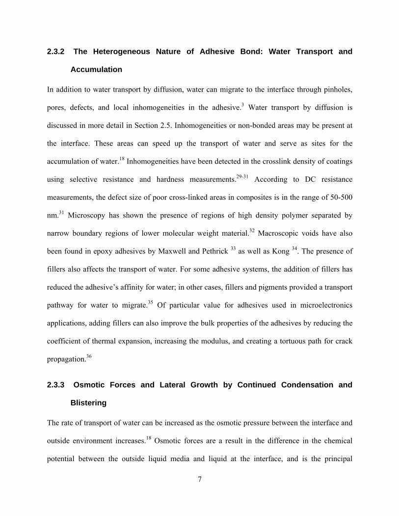
2.3.2 The Heterogeneous Nature of Adhesive Bond: Water Transport and

Accumulation

In addition to water transport by diffusion, water can migrate to the interface through pinholes,

pores, defects, and local inhomogeneities in the adhesive.3 Water transport by diffusion is

discussed in more detail in Section 2.5. Inhomogeneities or non-bonded areas may be present at

the interface. These areas can speed up the transport of water and serve as sites for the

accumulation of water.18 Inhomogeneities have been detected in the crosslink density of coatings

using selective resistance and hardness measurements.29-31 According to DC resistance

measurements, the defect size of poor cross-linked areas in composites is in the range of 50-500

nm.31 Microscopy has shown the presence of regions of high density polymer separated by

narrow boundary regions of lower molecular weight material.32 Macroscopic voids have also

been found in epoxy adhesives by Maxwell and Pethrick 33 as well as Kong 34. The presence of

fillers also affects the transport of water. For some adhesive systems, the addition of fillers has

reduced the adhesive’s affinity for water; in other cases, fillers and pigments provided a transport

pathway for water to migrate.35 Of particular value for adhesives used in microelectronics

applications, adding fillers can also improve the bulk properties of the adhesives by reducing the

coefficient of thermal expansion, increasing the modulus, and creating a tortuous path for crack

propagation.36

2.3.3 Osmotic Forces and Lateral Growth by Continued Condensation and

Blistering

The rate of transport of water can be increased as the osmotic pressure between the interface and

outside environment increases.18 Osmotic forces are a result in the difference in the chemical

potential between the outside liquid media and liquid at the interface, and is the principal

8

mechansim for blistering in coatings.3,37 Osmotic pressure and subsequent blistering is promoted

by the presence of hydrophilic sites or salts which decreases the equilibrium vapor pressure and

promotes condensation.38 Early work by Kittleberger and Elm showed that water penetration

through an alkyd coating was a function of osmotic pressure.39 Work by Perera and Heertjes, and

Kinsella and Mayne showed for a variety of polymer coatings that water diffused by an osmotic

pressure gradient. 29,40 Van der Meer-Lerk and Heertjes observed that even if these differences in

activity were small, blisters would continue to grow, the implication being that even minute

amounts of contaminants at the surface can result in blistering. 41 The formation of water clusters

can accelerate the blistering process by absorbing ionic species from the adhesive or substrate,

further increasing osmotic pressure.37

2.3.4 Physisorption of Water at the Interface

It is accepted that when water reaches the interface between an adhesive and an untreated high-

energy substrate, the adhesive bonds attributable to secondary molecular interactions (van der

Waals, hydrogen), are disrupted immediately.3 Furthermore, the work of adhesion between the

polymer and a high energy substrate, in the presence of water, is negative. In other words, the

force between the two adherends becomes repulsive. However, it should be noted that when

covalent bonding, interdiffusion, and/or mechanical interlocking are present, the work of

adhesion can not be used to explain adhesive failure.

2.4 Methods to Increase the Lifetime of Adhesive Bonds

From the above evidence, if adhesion forces are attributable to only secondary or van der Waals

forces, then adhesion strength will be poor in the presence of water. Moreover, the problem is

9

exacerbated by temperature. Two general strategies are suggested to improve the durability of

adhesive joints:13

1. Preventing water from reaching the interface in sufficient quantity

2. Improving the durability of the interface itself

Selection of the appropriate adhesive or chemical modification of the adhesive can reduce the

permeability and diffusivity of water into the adhesive joint. Because water transport in the bulk

is strongly related to free volume, the absorption of water may be reduced by introducing

crystallinity or by increasing the crosslink density, both of which lower free volume. Water

permeation can be reduced by decreasing the polymer’s affinity for water; for example, by

reduction of the number of polar or hydrophilic groups. In addition, water absorption may be

reduced by adding fillers to the polymer which may effectively act as a barrier to moisture

intrusion.

For metals substrates, inhibitors may be added to retard the hydration of oxide layers at

the adhesive-substrate interface. For glass and metals, silane coupling agents are used as a

primer, forming a hydrophobic poly(siloxane) network on the surface of the substrate.42 An

exceptional review of the role of silane coupling agents on epoxy adhesion can be found in the

work of Whittle et al.43 As referenced earlier, moisture resistance can be improved if covalent

bonds, interdiffusion, and/or mechanical interlocking are present at the interface. Surface

roughening can also increase the surface energy of the substrate, providing a longer path of

diffusion for the water to travel along the interface, and promoting mechanical interlocking in

some cases. Following the arguments of Leidheiser and Funke, to improve adhesive durability, a

suitable strategy would be to reduce the number of non-bonded areas, which may act as a

nucleus for further debonding. This is supported by a conversation with Professor Henry

10

Shreiber.44 He suggested that to improve adhesive durability, the number of covalent bonds at the

interface should be increased. This would effectively reduce the space at the interface for water

to reside, as well as require a hydrolysis reaction for debonding. Limiting the presence of water

at the interface slows down the process of corrosion, hydrolysis, and other mechanisms of joint

degradation. Therefore we might expect a correlation between dry adhesion and the durability of

adhesive joints in aggressive environments.

2.5 Diffusion in Polymers and Adhesive Joints

2.5.1 Fickian Diffusion

The diffusion of a penetrant (either a fluid or gas) through many materials can be modeled using

Fick’s second law of diffusion (typically referred to as simply Fick’s Law):

Equation 2-1 2

2

xCD

tC

∂∂

=∂∂

where C is the concentration (g cm-3) of penetrant or absorbed fluid, t is time (seconds) and x is

position (cm) and D is the diffusion coefficient or diffusivity of the penetrant in the polymer.45

The diffusion coefficient is characteristic of the rate of a penetrant transport for a specific

penetrant-host material combination. Fickian diffusion is an ideal case that assumes the

absorption process is independent of concentration and temperature. The diffusion takes place by

random jumps (or random walk) of the penetrant molecule in the polymer with little interaction

with the polymer matrix. In this case, the rate of relaxation of the polymer matrix is faster than

the rate of penetrant diffusion. Fickian diffusion is more common in rubbery materials that have

flexibility and mobility, larger free volumes, and have relatively fast relaxation times. In glassy

materials the rate of relaxation of the host matrix is much slower than the absorption process. In

11

this case, deviation from ideal Fickian diffusion, or even “non-Fickian” diffusion (see below)

may occur and Fick’s second law is no longer applicable.

The most common method for characterizing absorption processes and calculating the

diffusion coefficient is by a mass-uptake experiment. In most mass-uptake experiments, the

mass-gain of penetrant as a function of exposure time of a thin free-standing film is measured

using a mass balance. These data can then be fit to Fick’s second law provided an equilibrium

mass-uptake value is reached. Leidheiser and Funke 18 and Nguyen et al. 3 point out that for

coatings and composite materials, more relevant mass-uptake results should use the coating or

composite itself, rather than a free-standing film of the same material.

For a free polymer film of thickness 2L with a uniform initial concentration (C0) and the

surface is kept at a uniform concentration (CS), the solution to Fick’s Law in terms of

concentration is 45:

Equation 2-2 ⎟⎠⎞

⎜⎝⎛ +

⎥⎦

⎤⎢⎣

⎡ +−

+−

−=−− ∑

∞

= Lxn

LtnD

nCCCtxC

n

n

S 2)12(cos

4)12(exp

12)1(41

),(0

2

22

0

0 πππ

where C(x,t) is the concentration of penetrant in the polymer at any time t and distance x. The

solution to Fick’s Law can be put in terms of the average mass of the substance diffusing in the

polymer by integrating Equation 2-2 across the thickness 2L of the free polymer film.46 Note that

the expression for the concentration as a function time and distance for diffusion in a bilayer film

can be found in the work of McKnight and Gillespie.47

The relative mass uptake Mt /M∞ can be expressed as:

Equation 2-3 ∑∞

=∞⎥⎦

⎤⎢⎣

⎡ +−

+−=

02

22

22 4)12(exp

)12(181

n

t

LtnD

nMM π

π

12

Where Mt is the mass of absorbed fluid at any time t and M∞ is the equilibrium or final mass of

absorbed fluid. The relative mass uptake is the scaled average water concentration; a fraction

ranging from zero at t = 0, to one at t = ∞.

2.5.2 Non-Fickian Diffusion

It is not unexpected to observe non-Fickian behavior with glassy polymers. A prominent feature

of non-Fickian diffusion is that there is no characteristic equilibrium (long time) mass-uptake

value (M∞). There are two general cases of non-Fickian diffusion: two-stage absorption and Case

II diffusion. Two-stage absorption is typical for polymers that exhibit structural relaxation

induced by the adsorption of the penetrant.48 In this case, the relative mass uptake curve is

composed of two stages, an initial fast Fickian absorption, followed by a slow non-Fickian

absorption that on the typical time scale of an experiment, never asymptotes. In some cases, such

as in epoxies and other polymers, water will absorb in two stages, but for different reasons than

mentioned previously: the first stage entails an interaction with a specific binding site

(sometimes referred to as bound water), followed by a second stage association in a liquid like

structure (sometimes referred to as non-bound water).49 Case II is another form of non-Fickian

diffusion characterized by a step-like concentration profile with a sharp diffusion front. In this

model, the diffusion occurs faster in the swollen material and the relative mass uptake appears

linear with time. Note that for Fickian diffusion, the relative mass uptake appears linear with the

square-root of time. Solutions of the relative mass uptake as a function of time for two-stage

absorption 48,50,51 as well as Case II 52 can be found in the literature.

If however, dramatic changes in the relative mass uptake are observed, then this

indicative of damage to the adhesive. A large mass loss may often be attributable to leaching of

13

the adhesive. A large mass gain in composites or adhesive coatings would be indicative of fluid

accumulation at the interface of the matrix, the filler or between the adhesive and substrate.

Although Fickian behavior is not typically observed in glassy materials, there are cases

where glassy polymers behave like porous materials and take on Fickian behavior - diffusion of

penetrant into free spaces in the polymer being responsible.46 Two stage absorption has also been

observed in epoxies presumably due to the formation of microcracks and crazes.1,2

2.5.3 Interfacial Diffusion and Diffusion in Adhesive Joints

A review of the available literature on interfacial diffusion reveals that, in general, the rate of

interfacial diffusion, or the presence of fluid at the interface becomes more critical to the lifetime

of the adhesive joint as the strength of the adhesive interface decreases. For adhesives bonded to

high energy substrates, and in the presence of water, this is especially true. For “weak”

interfaces, where secondary bonds forces dominate the adhesion, failure occurs almost

immediately as water contacts the interface. It is possible for water to be present in the bulk and

interface of the adhesive yet the integrity of the adhesive bond can be preserved if the interface is

“strong”. This is the case where covalent bonds are present. For strong interfaces, the role of

interfacial diffusion becomes less important and the rate limiting step for failure becomes the

chemical reaction at the interface. Davis et al., utilizing the technique of electrochemical

impedance spectroscopy, observed this behavior in epoxies bonded to aluminum with surface

preparations that resulted in either a weak or strong interface.18,20 They observed that the rate of

crack growth was slow for strong interfaces, but for weak interfaces crack growth was detected

almost immediately as moisture appeared at the interface and resulted in a fast rate of crack

growth.

14

Diffusion into adhesive joints was studied by Zanni-Deffarges and Shanahan by

comparing the calculated diffusion rates between non-bonded adhesive specimens and bonded

adhesive joints.53 They observed that the diffusion coefficient of the adhesive joint was greater

than that of the bulk adhesive. They conclude that the diffusion rate at the interface was greater

than in the bulk adhesive and hypothesize the phenomena of “capillary diffusion” where (at the

diffusion front) the higher surface energy of the dry adhesive effectively “pulls” moisture along

the interface. Furthermore, they mention the effect of adhesive shrinkage at a constrained

interface may result in dilation of the adhesive near the interface.

Nyugen et al. 54 and Linossier et al. 22 have also compared diffusion rates between bulk

specimens and adhesive joints using Fourier transform infrared spectroscopy in the multiple

internal reflection mode (FTIR-MIR). They detected significant diffusion at the interface for

poorly adhered adhesive systems where adhesion forces are governed by secondary interactions.

Vine et al. 55 studied the moisture uptake of an epoxy bonded to aluminum adherends

with various surface treatments. They observed faster diffusion in three-layer sandwich

specimens than predicted, based on mass-uptake experiments performed on bulk diffusion

specimens. They attributed this behavior to the presence of micro-cavities in the adhesive layer

and site work by Nyugen et al., Zanni-Deffarges and Shanahan, and Linnosier et al. as evidence

for diffusion at the interface as possibly faster than in the bulk.

The label “interfacial impedance spectroscopy” was coined by Takahashi and Sullivan to

refer to impedance measurements made at the surface or interfacial region of a coated

substrate.23,24 They detected changes in the frequency dependent complex impedance (Z*)

associated with the accumulation of moisture at the interface resulting from adhesive debonding.

15

They estimate that the size of the aqueous film to be at least 1 nm thick. However, from their

studies, information about the rate of moisture absorption at the interface was very limited.

2.5.4 Diffusion in Epoxies

2.5.4.1 Moisture Diffusion in Epoxies

Moisture diffusion in epoxies and other polymers is associated to the availability of molecular-

sized holes within the polymer and the polymer-water affinity.56 Water molecules in epoxies and

polymers can also be classified as either unbound or bound as discussed above.56 Unbound water

resides in the free-volume of the polymer and this does not cause dimensional changes in the

polymer. Bound water interacts with the polymer via hydrogen bonding and can result in

swelling and plasticization of the polymer. Therefore, unbound water is associated with the first

stage of two-step diffusion and bound water is associated with the non-Fickian second stage of

two-step diffusion.

It is generally accepted that moisture diffusion in many polymers is strongly correlated to

the free volume.57,58 This appears to not be the case in epoxies. Soles and coworkers found in

amine cured resins no correlation between the topology (nanovoid size and total volume of

nanovoids) and moisture transport.59 Although they found that moisture traveled through the

epoxy and gained access to hydrogen bonds via the nanovoids, it appears the nanopores do not

appear to be rate limiting. They point to local scale motions in the glassy state associated with

the β–relaxation as the rate-limiting step for moisture transport.

2.5.4.2 Water as a Plasticizer

A great deal of information has been accumulated on the role of water in epoxies, specifically the

diglycidyl ether of bisphenol A (DGEBA). In general, water can be viewed as “an efficient

16

homogeneous plasticizer that depresses the glass transition of the polymer”.60 However, given

the highly polar nature of water, plasticization of water can not be treated as a simple

superposition of the individual response of the polymer matrix and diluent. Controversy

surrounds the nature of site specific interactions between the absorbed water and the hydrogen

bonds of the host epoxy matrix. Banks and Ellis proposed that plasticization is attributable to an

increase in segmental motion and the disruption of hydrogen bonding network in the epoxy.61

Jelinski et al. have shown the contrary using NMR; while recognizing site specific interactions,

at room temperature there is likely no disruption of the hydrogen-bonding network, and that

water acts simply as a plasticizer.62 Furthermore, at ambient temperatures and above the average

thermal energy of the system can exceed the energy due to local polarization, reducing the

likelihood of site-specific interactions.60 Recently, additional NMR work by Luo and co-workers

have shown that, although moisture reduces the glass transition temperature of epoxies, the

presence of moisture has no effect on polymer mobility at temperatures below the glass transition

temperature.63

17

3 ADHESIVE STUDIES USING THE SHAFT-LOADED

BLISTER TEST

3.1 Introduction

The shaft-loaded blister test (SLBT) was used to characterize the strain energy release rate (also

commonly referred to as the adhesive fracture energy), G, of adhesive coatings. This research is

divided into the following sections:

1. Measuring the applied strain energy release rate of a pressure sensitive adhesive tape

and investigating the fracture mechanics model.64

2. Measuring the applied strain energy release rate of a model epoxy36 bonded to quartz

as function of relative humidity.

3. Adapting the SLBT for sub-critical fracture testing. The sub-critical fracture behavior

of the model epoxy bonded to silicon wafers substrates as a function of relative humidity

was measured. The sub-critical fracture behavior of a commercial filled epoxy (L4)

bonded to silicon wafers in water as a function of temperature was also investigated.

18

3.2 Strain Energy Release Rates of a Pressure Sensitive Adhesive

Tape Measured by the Shaft-Loaded Blister Test

(The Journal of Adhesion, 79: 69-97, 2003)

3.2.1 Abstract

The elastic solution to the shaft-loaded blister test (SLBT) was adopted to measure the applied

strain energy release rate (G) of Kapton® pressure sensitive adhesive (PSA) tape bonded to a

rigid substrate. The substrates used were either aluminum or Teflon®, a high-energy surface and

low-energy surface, respectively. The values of G were calculated from three different equations:

(1) load-based, (2) hybrid, and (3) displacement-based. An experimental compliance calibration

was utilized to measure the film’s effective tensile rigidity (Eh)eff, the results of which are

presented in an appendix. Plastic deformation at the contact area of the shaft tip and adhesive

results in an overestimated displacement (w0) (relative to the elastic model) leading to

disagreement among the values of G calculated. Estimation of the effective membrane stress in

the film, (Neff), as well as the reasonable agreement between the value of (Eh) determined from a

stress-strain experiment and the compliance calibration suggest that, in spite of the plastic

deformation, the assumption of linear elasticity in the crack growth region, and hence the validity

of the model, is reasonable. The compliance calibration has been shown to improve the

agreement among the values of G calculated from the three equations. Using the load-based

equation, the assumed “correct” value of G may be obtained for a thin adhesive coating

independent of the film’s stiffness even in the presence of plastic deformation at the shaft tip.

Comparing the value of G obtained by a pull-off test and the 90° peel test for a single ply

indicates that the value of G obtained by the SLBT is of reasonable magnitude, being less than

19

that obtained by the more firmly established pull-off test, and also that undesirable plastic

deformation is reduced relative to the 90° peel test. An experimental configuration for studying

the effects of liquids on the fracture energy has been demonstrated for the SLBT. This study

indicates that the SLBT is an attractive and convenient test method for measuring the strain

energy release rate of adhesive films, because of the insensitivity of the load-based equation to

the coating stiffness, plus the independence of the value of G on the plastic deformation at the

shaft tip, and the reduced plastic deformation at the crack front relative to the 90° peel.

Key words: strain energy release rate, pressure sensitive adhesive tapes, shaft-loaded blister test,

pull-off test, peel test, plastic deformation, environmental degradation, Kapton®

3.2.2 Introduction to Adhesive Testing of Thin Coatings

3.2.2.1 The Peel Test and Pull-off Test

Measuring the adhesion of many important thin coatings is difficult given their small load-

bearing capacity, associated with the thinness, and their relatively strong adhesion.65 These

conditions often lead to the film rupturing before debonding can occur. Even if film rupturing is

absent and delamination is successful, significant film plastic deformation may result. In this

case, calculations of the fracture toughness of the adhesive bond, or the applied strain energy

release rate (G), may not reflect the intrinsic adhesion strength due to the additional energy

consumed by the bending and stretching of the adhesive coating. For example, Kim et al has

reported that measured peel forces may be one hundred times greater than the actual adhesion

strength.66

20

Thin adhesive coatings are commonly and conveniently tested using the peel test. For a

linear elastic coating of large tensile stiffness and small bending stiffness, the strain energy

release rate can be expressed as follows 67:

Equation 3-1 ( )θcos1−=bPG

where b is the width of the film, P is the load, and θ is the angle between the peel arm and the

substrate. In practice, the peel force also depends on plastic dissipation within the coating, which

is a function of the angle (or geometry) and stiffness and/or thickness of the peel arm along with

the resulting stresses generated during bending and stretching the film. As a consequence,

Equation 3-1 has no utility beyond comparing the adhesion of nominally identical films loaded in

identical fashion.68 Gent and Kaang have observed higher strain energy release rates obtained

from the 180° peel test relative to the 90° peel test due to larger bending stresses.69 Conversely,

at small peel angles significant energy is stored due to the tensile stresses and stretching of the

film. Gent and Kaang suggest using an angle of 45° and limiting the tensile strain to below 10-

15%; under their conditions, less than a 20% increase in the peel force resulted compared to the

extrapolated intrinsic adhesive strength.

Film rupture during peel testing can occur not only from the high stresses generated but

also from the use of mechanical grips. A typical solution is to employ a backing or reinforcement

layer to strengthen the adhesive coating; however, the additional reinforcement can change the

stiffness of the peel arm and the subsequent peel force. Gent and Hamed showed that for very

thin films of Mylar®, which yield substantially during peeling, as the adhesive coating thickness

increased, the peel force also rises due to an increase in the strain energy.70 However, a further

increase in the thickness showed that the peel forces were reduced as the stiffness of the film

21

increased. This latter effect was attributable to an increase in film yield stress, and a reduction in

bending stresses, which is consistent with what was shown by Kim et al.66 A critical thickness

was observed beyond which no further change in the peel force was observed as the thickness

was increased.

Given that the peel force and corresponding value of G depend on the energy consumed

during plastic deformation of the adhesive, efforts have been made to determine an intrinsic

adhesive fracture energy by considering the energy dissipated during tensile deformation and

bending of the peel arm, in addition to the energy stored in the peel arm. Kinloch et al. utilized

this approach to calculate Ga, a ‘geometry independent’ parameter, independent of the peel angle

and thickness of the adhesive.71 Moidu et al. developed an analytic approach to determine the

plastic deformation in the adhesive and also studied the effects of adhesive constitutive

properties and peel angle. 72,73

Ideally, for thin coatings an adhesion test should reduce the above discussed misleading

effects of the angle and stiffness of the peel arm, reduce plastic deformation, and eliminate the

use of mechanical grips. In addition, a procedure for reinforcing the film without significantly

affecting the measured peel force would be beneficial. A test that, in general, meets these

requirements is the pull-off test 74, or V-peel test 75, illustrated in Figure 3-1. In this experiment,

to initiate debonding, a force is applied by a pin placed perpendicular to and in the center of a

strip of coating. From the peel force and angle of debond the strain energy release rate can be

determined from Equation 3-2.

Equation 3-2 b

PG θ83

=

22

Gent and Kaang showed that the value of Gc obtained from the pull-off test was independent of

the film stiffness.74 The value of Gc was also significantly less than that obtained by the 90° peel

test due to the small angle of deflection between the peel arm and substrate (< 25°), which led to

a decrease in the plastic deformation arising to bending stresses.

3.2.2.2 Blister Tests

Another broad category of tests that eliminates the use of grips and reduces plastic deformation

due to bending (due to the small angle between the peel arm and substrate) are the blister tests.

Blister specimens consist of a thin film adhered to a substrate that has a hole in its center. The

development of the first blister test is credited to Dannenburg.76 However, not until the work of

Williams was the circular blister geometry adopted.77 In the standard or pressurized circular

blister test, either a liquid or gas is pressurized through the hole against the underside of the

coating until a blister crack is formed. The strain energy release rate can be calculated from the

relationship between the pressure, blister radius, and blister height. Similar to the pull-off test, it

has been shown that the strain energy release rate for the blister test is independent of the

stiffness of the film and specimen geometry.78 However, a disadvantage of the standard blister is

that the strain energy release rate increases as the blister radius increases, which could lead to

uncontrolled catastrophic debonding.79 To circumvent the problem of uncontrolled failure, a

constant strain energy release rate test, the “constrained blister” was proposed by Napolitano et

al. 80 and Chang et al. 81. Allen and Senturia proposed an island blister test to reduce stresses on

the film, enabling high strain energy release rates at relatively low pressures; however, a

drawback of the island blister is that uncontrolled debonding can still occur.82,83 Dillard and Bao

extended this to an additional constant strain energy release rate test, the peninsula blister.84 Wan

23

also developed a blister test that eliminates catastrophic debonding by utilizing a fixed amount of

the pressurizing gas, where the increase in pressure is driven thermally.85,86

3.2.2.3 Blister Tests for Environmental Studies

The blister test geometry also has a number of advantages when used for testing adhesives

subjected to environmental stress (time, temperature, and fluid). Specimens where the adhesive

is sandwiched between two impermeable adherends expose only an edge to the environment,

increasing the time necessary to saturate the adhesive and degrade the interface. Open face

specimens such as peel specimens can considerably reduce the exposure time before deleterious

effects of the environment are observed.87,88 However, the interfacial degradation may be more

pronounced at the sample edge, which can produce misleading results. For such environmental

degradation tests, blister specimens have several advantages: 1) the pressurizing medium can be

the degrading fluid of choice, 2) the blister axisymmetric geometry eliminates edge effects, and

3) direct exposure or diffusion of the fluid occurs perpendicular to the debond front.

3.2.2.4 Shaft-Loaded Blister Test

In this research, we explore the shaft-loaded blister test (SLBT), which utilizes the controlled

displacement of a spherically capped shaft, driven by a universal testing machine (UTM), as an

alternative to applying fluid or gas media. Malyshev 89 was the first to explore this test geometry

and derived the strain energy release rate for a pure bending plate boundary condition. Wan and

Mai developed an analytic solution to derive the strain energy release rate for a pure stretching

elastic film in a conical geometry and provided additional analysis that accounts for plastic

yielding at the contact area of the shaft tip.90 This elastic solution was adopted to measure the

adhesion of nylon to aluminum.91 Wan analyzed the transition from a bending plate to a

24

stretching membrane condition in the shaft-loaded blister test geometry.92 Wan and Liao

adopted the shaft-loaded blister test for measuring the constitutive properties of thin films from

the load vs. displacement data prior to debonding.93 In addition, delamination under cyclic

loading conditions was studied using the shaft-loaded blister test.94

Utilizing the elastic analytic model proposed by Wan and Mai90, we have adopted the

shaft-loaded blister test in order to investigate the adhesion of Kapton® pressure sensitive

adhesive tape bonded to a rigid substrate. The substrates reported here is either a low-energy

surface (Teflon®), or a substrate with a high-energy surface (aluminum). The model was tested

and the effects of film plastic deformation were probed by examining the value of G calculated

from three different equations, which will be termed: (1) load-based, (2) hybrid, and (3)

displacement-based. The effect of changing the stiffness of the coating while keeping the actual

interfacial adhesion constant was investigated by varying the number of plies of PSA tape

bonded to the aluminum substrate. The strain energy release rates obtained by the SLBT for a

single ply film are compared to the more conventional pull-off test and 90° peel test. An

experimental compliance calibration method for in-situ measurement of the film mechanical

properties was also obtained based upon blister crack growth data, and in order to preserve the

continuity of the paper, is discussed in an appendix. The great utility of the shaft-loaded blister

test in environmental exposure testing was demonstrated for several fluids and described below.

3.2.3 Shaft-Loaded Blister Test Theory

In this proposal, we explore the shaft-loaded blister test shown in Figure 3-2. The analytical

solution to the shaft-loaded blister by Wan and Mai90 is based largely on three assumptions: 1)

that the film undergoes pure elastic stretching in the radial and tangential directions, or in other

words, no that there is no contribution to the stiffness from bending, 2) the load is approximated

25

as a point load, which results in a conical blister profile, and 3) the angle between the adhesive

and substrate is shallow (less than 25°). Based on these assumptions Wan and Mai first arrive at

the following relation:

Equation 3-3 30

eff2

4)( wEhPa ⎟

⎠⎞

⎜⎝⎛=π

where a is the radius of debonding, w0 is the central shaft displacement, P is the load, E is the

Young’s tensile modulus, and h is the thickness of the backing. Collectively, (Eh) is commonly

referred to as the film’s tensile rigidity, which defines the film stiffness. (Eh)eff is the effective

tensile rigidity determined from a compliance calibration. Equation 3-3 is modified from the

original work of Wan and Mai- we take the liberty of replacing (Eh) with (Eh)eff, and also utilize

equation 3 to carry out a compliance calibration. The results from application of Equation 3-3 are

presented and discussed in the Appendix of this section.

Utilizing Equation 3-3 and an energy balance derived from linear elastic fracture

mechanics, Wan and Mai arrive at the following three expressions for the strain energy release

rate:

Equation 3-4 3/43/1

4161

⎟⎠⎞

⎜⎝⎛

⎟⎠⎞

⎜⎝⎛=

aP

EhG

π

Equation 3-5 2

02

1⎟⎟⎠

⎞⎜⎜⎝

⎛=

wP

EhG

π

Equation 3-6 4

0

16⎟⎠⎞

⎜⎝⎛=

awEhG

26

During stable crack growth a, w0, and P are predicted to increase linearly. From the slope of

either P vs. a, P vs. w0, or w0 vs. a, the value of G can be calculated from Equation 3-4, Equation

3-5, and Equation 3-6 respectively. Examination of these three equations reveals that the value of

G calculated from Equation 3-4 depends strongly on the measured load (P), and the G calculated

from Equation 3-6 depends strongly on the measured displacement (w0). The debond radius (a) is

eliminated from Equation 3-5 a hybrid form involving both load and displacement. As a

consequence Equation 3-4, Equation 3-5, and Equation 3-6 are referred to as the load-based,

hybrid, and displacement-based equations, respectively.

The film tensile rigidity (Eh) can be determined from either an independent stress-strain

experiment or from a compliance calibration with the SLBT fixture. The initial linear

relationship of the stress–strain experiment yields the Young’s modulus, E. For the PSA tape

used in our research, the area and stress are calculated based only on the thickness of the backing

(Kapton®), not the soft adhesive layer. The tensile rigidity calculated as described from the

stress-strain data is denoted as (Eh)UTM. On the other hand, if the adhesive system closely

follows the assumptions of the analytic model, then fitting the experimental data to Equation 3-3

allows a compliance calibration which will then independently determine the effective film

tensile rigidity (Eh)eff. We note that a plot of P a2 vs. w03 should yield a straight line with a slope

equal to π (Eh)eff / 4. For several reasons this effective tensile rigidity (Eh)eff may be more

representative of the adhesive film’s mechanical properties than the film tensile rigidity

determined from the Young’s modulus and the film thickness, (Eh)UTM. Most importantly, the

effective tensile rigidity (Eh)eff can account for such effects as the difference in loading between

the uniaxial stress-strain experiment and the biaxial stress the film experiences in the actual

blister test configuration. In addition, the effects of the Poisson ratio, shear loading, anisotropy,

27

as well as the co-existence of bending and stretching stresses may be significant and could be

accounted for by the (Eh)eff method. Overall, this technique is similar to the compliance method

often adopted for the double cantilever beam specimen.95

To estimate the stress in the adhesive film, the effective membrane stress (Neff), is given

by Wan and Mai as:

Equation 3-7

2/122/1

eff 43log)(⎥⎥⎦

⎤

⎢⎢⎣

⎡+⎟

⎠⎞

⎜⎝⎛=

raGEhN

where r is the radial distance from the center of the blister. Membrane stress is defined as the

stress multiplied by the film thickness, therefore Neff is not a “true” stress in the strict sense (load

per unit cross sectional area), but rather a force per unit width. Neff is composed only of the radial

and tangential stress components of the film, and ignores stresses due to bending, which may or

may not be significant. If Neff ≥ σy h, where σy is the adhesive yield strength, then membrane

yielding is predicted to occur. Examination of Equation 3-7 reveals that in the limit of r → 0, the

effective stress approaches infinity; thus, in the center of the blister we expect deviations from

simple elastic response. However, application of Equation 3-4, Equation 3-5, and Equation 3-6

requires that the assumption of linear elasticity hold true at the crack front, where r = a and Neff =

(3G(Eh) / 4)1/2. In the event that Neff ≥ σy h at the crack front, the elastic blister equations are

invalid. The solution for the case of a thin film experiencing plastic deformation in an inner

annulus and an elastic outer annulus has been developed also by Wan and Mai, but is not

discussed here.

28

3.2.4 Experimental

3.2.4.1 Materials

The PSA tape utilized in the experiments is Kapton® polyimide film tape with a total thickness

of 63.5 µm (2.5 mils). The PSA tape is a bilayer system consisting of a Kapton® backing, which

has a thickness of 25.4 µm (1 mil), and a pressure sensitive silicone-based thermosetting

adhesive, which has a thickness of 38.1 µm (1.5 mils). The base polymer used in silicone-based

PSAs is polydimethylsiloxane (PDMS)96 which has a glass transition at –125°C. The PSA tape

was bonded to either aluminum or Teflon®, a high energy and low energy surface, respectively.

The surface energies of Al2O3 and Teflon® are 574 and 19.1 mJ/m2, respectively.97 The

aluminum surface was treated with a caustic solution and rinsed with acetone prior to application

of the PSA tape. The Teflon® surface was also rinsed with acetone prior to application of the

PSA tape. The tensile modulus (E) of the Kapton® tape, calculated from ASTM D-882-91 using

the sample cross-sectional area based on the backing thickness, is roughly 3.05 +/- 0.06 GPa.

The stress-strain curve for the PSA tape is shown in Figure 3-3, and the yield strength σy was

calculated as 120 +/- 6 MPa using a bimoduli approximation.

3.2.4.2 Technique

A 0.8 cm diameter hole was bored into the aluminum and Teflon® substrates. The PSA tape

dimensions were 2.54 x 2.54 cm square. A ball-bearing 0.7 cm in diameter is mounted on the

shaft tip. The bonded PSA tape was attached face down in a rigid fixture. During the experiment,

a mirror and a transparent ruler were used to observe the debond radius with a video camera. To

account for the parallax error, a small correction was necessary. A schematic of the visual image

as seen through the video camera is shown in Figure 3-5. The load (P) and displacement (w0)

29

were recorded by the UTM and the shaft displacement rate was 0.1 mm/sec. The tests were

conducted at room temperature. This experiment is mechanically much simpler than the

pressurized blister test since the mechanically driven shaft eliminates the use of a pump, pressure

gauge, and valves. For the aluminum substrate, samples consisted of stacked, bonded, Kapton®

PSA tape either 1, 2, or 4 plies thick. The number of stacked films is designated as n. As a result,

the film thickness (h), based on the backing, is equal to 25.4 µm multiplied by n. A single ply

only was tested for the Teflon® substrate. The only criterion each sample must meet for

acceptable analysis is that the debond must occur roughly axisymmetrically. For comparison, the

strain energy release rate for a single ply of Kapton® PSA tape was also measured by the pull-

off test and the 90° peel test. For the pull-off test, G was calculated from Equation 3-2. For the

90° peel test, G was calculated from equation 1, which in this case simplifies to Equation 3-8.

Equation 3-8 bPG =

3.2.5 Results and Discussion

3.2.5.1 Aluminum Substrate

3.2.5.1.1 Shaft-Loaded Blister Test

The load (P) vs. shaft displacement (w0) curves obtained directly from the UTM are shown in

Figure 3-6 for n = 1, 2, and 4. There are three regions of interest: Region I, the pre-debonding

region at the beginning of the test where the blister begins to form, Region II, the stable crack

growth region where the crack begins to propagate once a critical load is reached (P*) and the

slope of P vs. w0 becomes linear, and Region III, where edge effects occur and the load begins to

decrease as the film debonds completely from the substrate. From the slope of P vs. w0 in the

30

stable crack growth Region II, the value of G may be determined using the hybrid equation

(Equation 3-5).

The debond radius (a) vs. shaft displacement (w0) data are shown in Figure 3-7 for n = 1,

2, and 4. From the slope of these lines, G may be determined using the displacement-based

equation (equation 6). During stable crack growth the relationship of the load (P) and crack

length (a) is also linear, but is not shown. From the slope of the load (P) vs. debond radius (a)

plot, G may be determined using the load-based equation (equation 4). As mentioned by Wan

and Mai, the non-zero intercept observed in Figure 3-6 and Figure 3-7 is a result of the finite

contact area between the shaft tip and adhesive film.

For n = 1, 9 samples were tested. For the n = 2 and 4 specimens we tested 4 and 3

samples, respectively, because fewer samples met the criteria of axisymmetric debonding. We

noted that as the thickness increased, the debond radius tended to be less symmetric and the

blister shape became roughly square, probably due to anisotropy in the film and to the increase in

the stiffness of the film. This effect was most noticeable in the n = 4 case. Evidence for the

anisotropy of the Kapton® backing can be found in an article by Park et al.98

Utilizing (Eh)UTM, the resulting calculated average values of G, determined from the

load-based, hybrid, and displacement-based equations, are presented in Table 3-1 for n = 1, 2,

and 4. For the load-based equation, the calculated values of G for different plies are in good

agreement. The hybrid and displacement-based equation both show good agreement when n = 1

and 2 but not for n = 4. G values from the displacement-based calculation are significantly larger

than those obtained by either the load-based or hybrid equation.

31

Table 3-1 Applied strain energy release rates (J/m2) for n = 1, 2, and 4 on aluminum calculated

from the load, hybrid, and displacement equations and (Eh)UTM

n Load (P/a) Hybrid (P/w0) Displacement (w0/a)

1 33.4 +/- 3.6 31.9 +/- 3.1 45.8 +/- 10.4

2 35.0 +/- 7.7 33.9 +/- 5.2 44.8 +/- 9.6

4 31.0 +/- 2.2 24.2 +/- 1.5 62.4 +/- 11.1

The discrepancy between the values of G calculated by either the load-based, hybrid

equation, or displacement-based equation is largely associated with the (visible) plastic

deformation at the contact zone between the shaft tip and PSA tape, where the stresses are

highest. Equations 3-6 are based on an elastic, conical blister profile (Figure 3-2); however, the

actual blister shape resembles that shown in Figure 3-8. As a result, the measured w0 is larger

than the theoretical, elastic, w0. This difference is especially significant in the displacement-

based equation where w0 is in the numerator and is raised to the 4th power. Error in w0 is less

significant in the hybrid equation where w0 is in the denominator and is raised to the 2nd power.

As a consequence, the value of G determined from the displacement-based equation is

significantly larger than the value of G calculated from the load-based or hybrid equation. In

contrast, the value of G obtained by the load-based equation, having no w0 term, is independent

of plastic deformation of the film around the shaft tip.

A visible dimple remaining in the PSA tape at the contact region of the shaft tip after

testing is evidence that significant localized plastic deformation or permanent set has occurred

during testing. Additional evidence that significant permanent set has occurred was also gathered

from the loading and unloading cycles, which were repeated six times. The area of contact

32

between the shaft tip and adhesive film was coated with chalk to reduce effects of the adhesive

film adhering to shaft tip. The substrate used for this experiment was polished aluminum, which

is different than the aluminum treated with caustic solution that was used in the previous

experiments. Although the adhesion strength is larger (≈71 J/m2) for this substrate than that of

the caustic solution treated aluminum surfaces (≈35 J/m2), the salient features of the loading and

unloading cycles are most probably similar. Figure 3-9displays the resulting graph of the load

(P) vs. displacement (w0) for each cycle. Each cycle displays an initial loading region (Region I)

followed by a brief zone of crack propagation (Region II) where the blister radius increased

approximately 0.5 – 1 mm. For each cycle, the characteristic signature of plastic deformation is

evident where the displacement does not immediately return to the origin once the load is

removed. Examination of Figure 3-9 shows that with each cycle, there is a progressive increase

in the amount of permanent set. The critical displacement (w0), where the load first begins to

rise, corresponding to the point where the shaft tip contacts the film, increases with each

subsequent cycle. However, during unloading when the shaft tip returns to zero displacement, the

PSA tape may partially re-adhere to the substrate. This can result in the load increasing

prematurely. It is therefore more meaningful to look at the value of displacement when the load

is completely removed as an indication of the permanent set that occurs. The final and maximum

load (PMax) of each cycle vs. the displacement when the load is completely removed is shown in

Figure 3-10. Figure 3-10 also shows that net amount of film yielding increases, which each

subsequent loading cycle; however, the rate at which yielding increases slows. Taken

collectively, the debonding regions (Region II) of each cycle appear to overlap in the same

fashion as expected for a single P vs. w0 curve in which a specimen is loaded in a typical fashion.

33

The inaccurate value of w0 (relative to the pure elastic case) and the resulting

disagreement between the values of G, obtained by Equation 3-4, Equation 3-5, and Equation

3-6, may raise questions about the validity of the basic assumption of linear elasticity for the

SLBT. To examine this, plots of Neff vs. r for different values of a were constructed as suggested

by Equation 3-7for n = 1, 2, and 4. As an example, the resulting plot for n = 1 is shown in Figure

3-11. We assume that if Neff ≥ σp h then plastic deformation occurs. The resulting plots reveals

that plastic deformation is predicted solely at the contact zone of the shaft tip (r ≤ 0.1 mm for n =

1), and that no plastic deformation (attributable to radial and tangential stresses) is predicted to

occur at the crack front ( r = a). These results suggest that the assumption of linear elasticity is

valid, if bending stresses are ignored.

Evidence of the adhesive-substrate system deviating from the assumptions of the model is

observed for the multiple stacked tape, where n = 4. As shown earlier, the effects of plastic

deformation here seem to be more pronounced; the value of G is either smaller or larger when

calculated from the hybrid and displacement based equation, respectively. This is unexpected,

given that the stiffer film should plastically deform the least, therefore plastic deformation is

probably not the most significant reason for the discrepancy. An alternative explanation is that

for n = 4 the adhesive system does not follow the assumptions of the model as closely as in the n

= 1 and 2 case. The thicker structure should result in the adhesive behaving more like a bending

plate and less like a stretching membrane. In addition, significant shear forces between the

stacked plies are possibly playing a role. This shear effect may contribute significantly given that

the four layered structure of Kapton® is interspersed with the soft PSA, and would reduce the

effective stiffness of the film. As mentioned earlier, the deviation from the model is supported by

the visual observation that increasing the film stiffness and anisotropy may cause the blister to be

34

less circular and adopt a square or non-symmetric debond pattern. However, when employing the

load-based equation, the similarity between the n = 4 case and the model is close enough to

obtain values of G close to those for to n = 1 and 2.

Rearrangement of the load-based, hybrid and displacement-based equations shows that

the slopes of (P / a), (P / w0) and (a / w0) plots should linearly scale with the variables h1/4, h1/2,

and h1/4 or n1/4, n1/2, and n1/4 respectively. Plots of such graphs using average slopes obtained

from the group of samples are shown in Figure 3-12. The error bars represent one standard

deviation. For the load-based equation, the predicted scaling behavior is followed, albeit the

relationship is not perfect. For the hybrid and displacement-based equation, the graphs show that

for n = 4 the scaling law fails, a result which may be attributable to reasons outlined previously.

The assumption of linear elasticity and hence the validity of the model is supported by

calculations of Neff. In addition, the agreement among the values of G obtained from the load-

based equation for n = 1, 2, and 4 (independent of the film stiffness) is further evidence

supporting the approach of Wan and Mai. It is not unexpected that the value of G obtained by

hybrid and displacement based equations do not agree with that obtained by the load based

equation given the plastic deformation at the shaft tip, unaccounted for by the elastic solution. If

we accept that plastic deformation is confined to the area at the shaft tip, and linear elasticity is a

valid assumption at the crack front (r = a), then we can assume that the load and blister radius

are in equilibrium and that the value of G obtained by the load-based equation is independent of

film yielding near the shaft tip and provides good values of G. This is confirmed by the

consistency of the values of G calculated using this method.

35

3.2.5.1.2 Alternative test geometries

The values of G for a single ply (n = 1) PSA tape which were obtained from alternative

test geometries (the pull-off test and the 90° peel test) are shown in Table 3-2. The tests were

performed at the identical crack propagation rate as that of the SLBT (10 mm/minute) in order to

reduce the viscoelastic differences at the crack tip. The value of G determined from the pull-off

test was of the same order of magnitude as that obtained using the SLBT when employing the

hybrid equation. The value of G determined from the 90° peel test was an order of magnitude

greater than these, probably due to plastic deformation of the tape, which may originate from the

bending stresses associated with the large angle of deflection between the peel arm and substrate.

These observations support our contention that the value of G obtained by the SLBT is valid, and

an especially attractive alternative to the 90° peel test. Similar to other low angle adhesion tests,

the SLBT may produce values of G that more closely reflect the intrinsic adhesion strength of an

adhesive system than do the high angle 90° and 180° peel counterparts. Both the pull-off test and

SLBT share similar angles of debonding (for n = 1), roughly 14° and 16° (estimated from θ =

arctan (w0 / a)), respectively, and so large differences in the localized stress at the crack front are

not expected. Although there may also be significant bending stresses associated with the SLBT,

given the similar angle of debonding between the SLBT and pull-off test, any bending stresses if

they are significant, may be similar in magnitude. Given the similarity between the pull-off test

and SLBT, and how well established the pull-off test is, further supports the utility of the SLBT.

36

Table 3-2 Applied strain energy release rates (J/m2) calculated from alternative test geometries

(n = 1).

Load based SLBT Pull-off Test 90° Peel Test

33 +/- 4 45 +/- 1 141 +/- 7

The assumption that the angle of debonding be less than 25°, used to derive the SLBT

model, is satisfied. Furthermore, this angle appears to be constant given the linear relationship

between the displacement (w0) and debond radius (a). It is also of interest to mention that the

SLBT, peel test, and pull-off test are all constant angle adhesion tests, and so they share the

characteristic of self-similarity, and a value of G that is independent of the crack length or length

of the peel arm.

3.2.5.2 Teflon® Substrate

3.2.5.2.1 Shaft-loaded blister test

Load (P) vs. displacement (w0), and crack length (a) vs. displacement curves (w0) were also

generated for a single ply (n = 1) of the PSA adhering to a low surface energy Teflon® substrate,

shown in Figure 3-13. Seven samples were tested. The resulting average values of G are listed in

Table 3-3; there, as expected for such a low surface energy substrate, the values are low.

Utilizing (Eh)UTM, the effects of plastic deformation are notable in this adhesive system; the

average values of G obtained by the hybrid and displacement-based equations were smaller and

larger, respectively, relative to the load-based equation. However, the value of G calculated by

the load-based and the hybrid equation agree within one standard deviation.

37

Table 3-3 Applied strain energy release rates (J/m2) for Kapton® PSA tape bonded to Teflon®,

n = 1, calculated from the load, hybrid, and displacement equations and (Eh)UTM

Load (P/a) Hybrid (P/w0) Displacement (w0/a)

17.6 +/- 3.4 15.5 +/- 1.5 21.8 +/- 4.2

3.2.5.2.2 Alternative Test Geometries

The value of G obtained from the pull-off and 90° peel tests from Teflon®, with equal crack

propagation rates, were approximately 60% greater than those found by the SLBT, see Table 3-4.

The agreement between the pull-off and 90° peel test is excellent. These results in conjunction

with the values of G obtained by the pull-off test for aluminum, suggest that the fracture energies

obtained by the SLBT, will be slightly less than obtained by the pull-off test. The agreement

between the pull-off and 90° peel suggests that plastic deformation of the peel arm due to

bending is reduced for the Teflon® - Kapton® combination. In sharp contrast, if the PSA tape is

adhered strongly (e.g., the aluminum substrate), the bending of the peel arm causes significant

plastic deformation when using the 90° peel geometry. Similar results were observed by Gent

and Kaang 74 for adhesives with weak interfacial adhesion. More significant discrepancy could

result as the film yield strength decreased or as the interfacial adhesion strength increased.

Table 3-4 Applied strain energy release rates (J/m2) for Kapton® PSA tape bonded to Teflon®,

n = 1, using alternative test geometries

Load based SLBT Pull-off Test 90° Peel Test

18 +/- 3 27 +/- 1 26 +/- 3

38

3.2.6 Effects of Fluids at the Interface

The effect of fluid added directly to the interfacial region during crack propagation was

investigated and is reported in terms of changes in of the applied strain energy release rate. For

these experiments, the reservoir between the PSA tape and aluminum substrate was filled with a

mixture of methanol and water, and the load was immediately applied. The reservoir eliminates

experimental difficulties associated with the complete fluid submersion of an adhesive specimen.

The methanol concentration was varied from 0, 40, 60, 80, to 100 wt. %. Tests were conducted at

room temperature. A schematic of the experimental configuration is shown in Figure 3-14. The

load (P) vs. displacement (w0) curves are shown in Figure 3-15. Table 3-5 lists the G values,

calculated using the hybrid equation and the (Eh)UTM, and P* for the respective methanol

concentrations. Good agreement between the value of G calculated from load-based and hybrid

equations and (Eh)UTM, for n = 1 and 2 bonded to aluminum, was noted. The presence of water (0

% methanol concentration) increased the value of G, or at least within reasonable error did not

have any measurable effect on the value of G. Furthermore, as the concentration of methanol

increases, the critical load where debonding begins (P*), and the slope of the P vs. w0 plot

decreases.

39

Table 3-5 Applied strain energy release rates (J/m2) calculated from hybrid equation for

Kapton® PSA tape (n = 1) with various concentrations of methanol in water (0, 40, 60, 80, 100

wt. %) and (Eh)UTM

methanol concentration G (J/m2) P* (N)

dry 36 9.6

0 % 38.3 8.7

40 % 31.6 8.7

60 % 29.3 6.7

80 % 27.8 5.2

100 % 6.9 0.1

Our results are similar to those obtained by Chaudhury and Whitesides for the adhesion

of PDMS surfaces in contact with mixtures of methanol and water.99 Utilizing the JKR model

and Young’s equation, they observed that the adhesion of PDMS surfaces in the presence of a

high surface energy fluid (γ = 72.94 at 20°C 100), water, was higher than in air. The work of

adhesion for PDMS was determined to be 43.6 mJ/m2 and 74 mJ/m2 in air and in water,

respectively. In the presence of a low surface energy fluid (γ = 22.5 at 20°C 100), methanol, the

adhesion of PDMS surfaces decreased to 6 mJ/m2. The observed reduction in adhesion strength

is attributable to the absorption of fluids on the surface; therefore, the lower the surface energy of

the fluid, the more readily the fluid can wet the surface and disrupt the bonds between the

adhesive and substrate.

40

3.2.7 Conclusions

We investigated the SLBT for its applicability in determining adhesive fracture energy of tapes

adhering to rigid substrates. Plastic deformation at the contact area of the shaft tip resulted in an

overestimated displacement, w0 (relative to the elastic model), resulting in discrepancy among

the values of G calculated by the load-based, hybrid, and displacement-based equations.

Estimation of the effective membrane stress (Neff) in the film suggests that, in spite of the plastic

deformation, the assumption of linear elasticity in the crack growth region, and hence the validity

of the model, seem reasonable.

As discussed in the appendix, a compliance calibration has been adopted to measure

(Eh)eff, which agrees reasonably well with (Eh)UTM in cases of one or two plies of tape. For more

layers of tape, the disagreement between (Eh)eff and (Eh)UTM is roughly 20%, but is not

unexpected given the large stiffness and multi-layered structure. The compliance calibration has

been shown to improve the agreement between the value of G among the load-based, hybrid, and

displacement-based equations, however this appears to be an artifact of the error in w0.

Using the load-based equation accurate values of G were obtained for a thin adhesive

coating independent of the film’s stiffness, even with plastic deformation at the shaft tip. The

insensitivity of this load-based equation to the film stiffness suggests the compliance calibration

is unnecessary. Comparing the value of G also obtained by a pull-off test and a 90° peel test for a

single ply suggests that our value of G obtained by the SLBT, although of reasonable magnitude,

is smaller than that obtained by the more firmly established pull-off test, and also that the plastic

deformation is reduced relative to the 90° peel test, presumably due to the low angle of

deflection between the peel arm and substrate. An experimental configuration for studying the

effects of liquids on the fracture energy has been demonstrated. This study indicates that the

41

SLBT, because of the insensitivity of the load-based equation to the coating stiffness, the

independence of the value of G on the plastic deformation at the shaft tip, and the reduced plastic

deformation at the crack front relative to the 90° peel is an attractive and convenient test method

for measuring the strain energy release rate of adhesive films. Because the value of G is

independent of the film stiffness, the SLBT could be advantageous for testing fragile thin films

that could benefit from the addition of a reinforcement layer.

3.2.8 Appendix: Experimental compliance calibration

3.2.8.1 Aluminum Substrate

An experimental compliance calibration was performed by fitting the experimental data to

equation 3. As predicted, the relation between P a2 vs. w03 (Figure 3-16) was linear and, from the

slope of the line, the effective film tensile rigidity (Eh)eff was calculated. A comparison of this

average (Eh)eff and the independently obtained (Eh)UTM is shown in Table 3-6. In all cases (n = 1,

2, and 4) the average (Eh)eff is less than the (Eh)UTM. For n = 1 the average (Eh)eff is about 9%

less than (Eh)UTM. The agreement is best for n = 2, the difference between the average (Eh)eff and

(Eh)UTM is 3%. The disagreement between (Eh)UTM and (Eh)eff for n = 4, about 20%, is not

unreasonable given the departure from the assumptions of the Wan’s model, attributable to

reasons discussed earlier: increased stiffness, anisotropy, and the multi-layered structure.

42

Table 3-6 Film tensile rigidity determined from ASTM D-882-91: (Eh)UTM, and from equation

3: (Eh)eff, as well as the number of samples tested

n (Eh)UTM N/m (Eh)eff N/m

1 77,500 70,600+/-6,300

2 154,900 150,800+/-11,600

4 309,800 252,100+/-17,200

Utilizing (Eh)eff, the average values of G, determined from the load-based, hybrid, and

displacement-based equations were calculated and are listed in Table 3-7 for n = 1, 2, and 4.

Using (Eh)eff , we note good agreement of G values between the load-based and hybrid equation

(Table III) irrespective of the number of plies. The disagreement observed when utilizing the

displacement-based equation is attributed to the plastic deformation and was discussed earlier. A

comparison of Table 3-1 and Table 3-7 reveals no significant difference between the values of G

measured using (Eh)UTM and (Eh)eff. However, more consistency was obtained when the

compliance calibration was utilized. When a compliance calibration was carried out for n = 2

virtually no difference in G values was observed, because of the small difference between

(Eh)UTM and (Eh)eff.

43

Table 3-7 Applied strain energy release rates (J/m2) for n = 1, 2, and 4 on aluminum calculated

from the load, hybrid, and displacement equations and the effective tensile rigidity: (Eh)eff

n Load (P/a) Hybrid (P/w0) Displacement (w0/a)

1 34.7 +/- 4.2 35.1 +/- 4.5 40.7 +/- 6.9

2 35.3 +/- 7.7 34.7 +/- 2.9 43.5 +/- 9.3

4 33.3 +/- 2.9 29.8 +/- 2.7 50.3 +/- 5.4

A larger value of w0, relative to the pure elastic case, will effect the value of (Eh)eff,

obtained by fitting the experimental data to Equation 3-3. Examination of Equation 3-3 reveals

that (Eh)eff ∝ w0-3. Therefore, the displacement, w0, which is overestimated if there is plastic

deformation would result in a calculated (Eh)eff which is less than that predicted in the case of a

purely elastic response. However, the effects of plastic deformation and the multi-layered

structure of the PSA tape would also effectively reduce the stiffness of the film and contribute to

the observation that (Eh)eff is less than (Eh)UTM. The ambiguities associated with the discrepancy

in w0 are also exacerbated by the similar and strong dependence of the value of G on both w0 and

(Eh) in the hybrid and displacement-based equations. Examination of the hybrid equation and

displacement-based equation reveals that G ∝ (Eh)-1 w0-2, and G ∝ (Eh) w0

4, respectively. The

load-based equation is less sensitive to the value of (Eh) relative to the hybrid and displacement-

based equation because G ∝ (Eh)-1/3. Because of the relative difference between the values of

(Eh)eff and (Eh)UTM, utilizing (Eh)eff rather than (Eh)UTM resulted in increasing the value of G

obtained by the hybrid equation and decreasing the value of G obtained by displacement-based

equation. The net effect is that the apparent results of plastic deformation are offset by a

corresponding reduction in the value of (Eh). This produced more consistent results when (Eh)eff

44

was incorporated into the calculations. This might lead to the conclusion that (Eh)eff better

describes the stiffness of the film and more closely reflects the mechanical propeties of the film

in the SLBT loading conditions as compared to (Eh)UTM. However, given the dependency on the

overestimated displacement, it is unlikely that the value of (Eh)eff truly reflects the mechanical

properties of the film loaded in the SLBT geometry, but is an artifact of the error in w0. In any

case, the linear fit of the experimental data to Equation 3-3, and the reasonable agreement

between (Eh)eff and (Eh)UTM (especially for n = 2) support the validity of Wan’s model and the

assumption of linear elasticity.

3.2.8.2 Teflon® Substrate

By fitting the experimental data to Equation 3-3an average (Eh)eff was calculated as 64,700 ±

7,100 N/m, approximately 17% less than (Eh)UTM. Using the experimental compliance

calibration, the average value of G was in good agreement among all three equations (Table 3-8).

Again, this is probably a result of the strong dependence of G on both (Eh) and w0 for the hybrid

and displacement equation, or it could be that (Eh)eff more closely reflects the mechanical

properties of the adhesive loaded in the SLBT conditions. If indeed (Eh)eff is reasonable, the

good agreement would not be unexpected given that the Teflon-PSA tape system complies well

with the assumptions of the model: namely, 1) the reduced bending stresses attributable to the

small thickness (single ply), and 2) the reduced interfacial adhesion strength, which reduces

stress and/or plastic deformation in the adhesive.

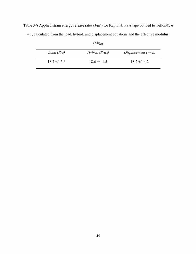
45

Table 3-8 Applied strain energy release rates (J/m2) for Kapton® PSA tape bonded to Teflon®, n

= 1, calculated from the load, hybrid, and displacement equations and the effective modulus:

(Eh)eff

Load (P/a) Hybrid (P/w0) Displacement (w0/a)

18.7 +/- 3.6 18.6 +/- 1.5 18.2 +/- 4.2

46

3.2.9 Figures

θ

P

substrate

adhesive film

Figure 3-1 Schematic of the pull-off test

P

w0

2a

hadhesive film

shaftsubstrate

P

w0

2a

hadhesive film

shaftsubstrate

Figure 3-2 Schematic of the shaft-loaded blister test

47

0

50

100

150

200

0 10 20 30 40 50 60Strain (%)

Stre

ss (M

Pa) σy

Figure 3-3 Stress-strain curve for Kapton® PSA

48

stand

shaft

adhesive film

video camera

mirror

transparent ruler

Figure 3-4 Schematic of the experimental set-up of the shaft loaded blister test

49

substrate adhesive film

ruler

Figure 3-5 Schematic of view of blister radius propagation

50

0

5

10

15

20

25

30

0 1 2 3 4

w 0 ( mm)

P (

N)

n = 1n = 2n = 4

0

5

10

15

20

25

30

0 1 2 3 4

w 0 ( mm)

P (

N)

n = 1n = 2n = 4

n = 1n = 2n = 4

n = 1n = 2n = 4

Figure 3-6 Load (P) vs. central shaft displacement (w0) for n = 1, 2 and 4

51

0

3

6

9

12

15

0 1 2 3 4

w 0 (mm)

a (m

m)

n = 1n = 2n = 4

Figure 3-7 Debonding radius (a) vs. central shaft displacement (w0) for n = 1, 2 and 4

52

P

wPlasticwElastic

area of plasticdeformation

Figure 3-8 Schematic of the actual blister profile

53

0

5

10

15

20

25

30

0 1 2 3 4

w 0 (mm)

P (N

)

Figure 3-9 Loading and unloading cycles for Kapton® PSA tape bonded to polished aluminum.

The loading portion of the curve is shown in filled symbols and the unloading portion is shown

in unfilled symbols.

54

0

5

10

15

20

25

30

0 0.5 1 1.5 2 2.5

w 0 (mm)

PM

ax (N

)

Figure 3-10 Plot of the final load PMax of each cycle vs. w0 for Kapton® PSA tape bonded to

polished aluminum.

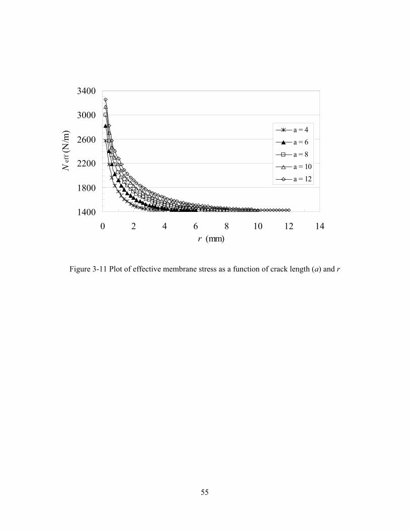
55

1400

1800

2200

2600

3000

3400

0 2 4 6 8 10 12 14r (mm)

Nef

f (N

/m) a = 4

a = 6a = 8a = 10a = 12

Figure 3-11 Plot of effective membrane stress as a function of crack length (a) and r

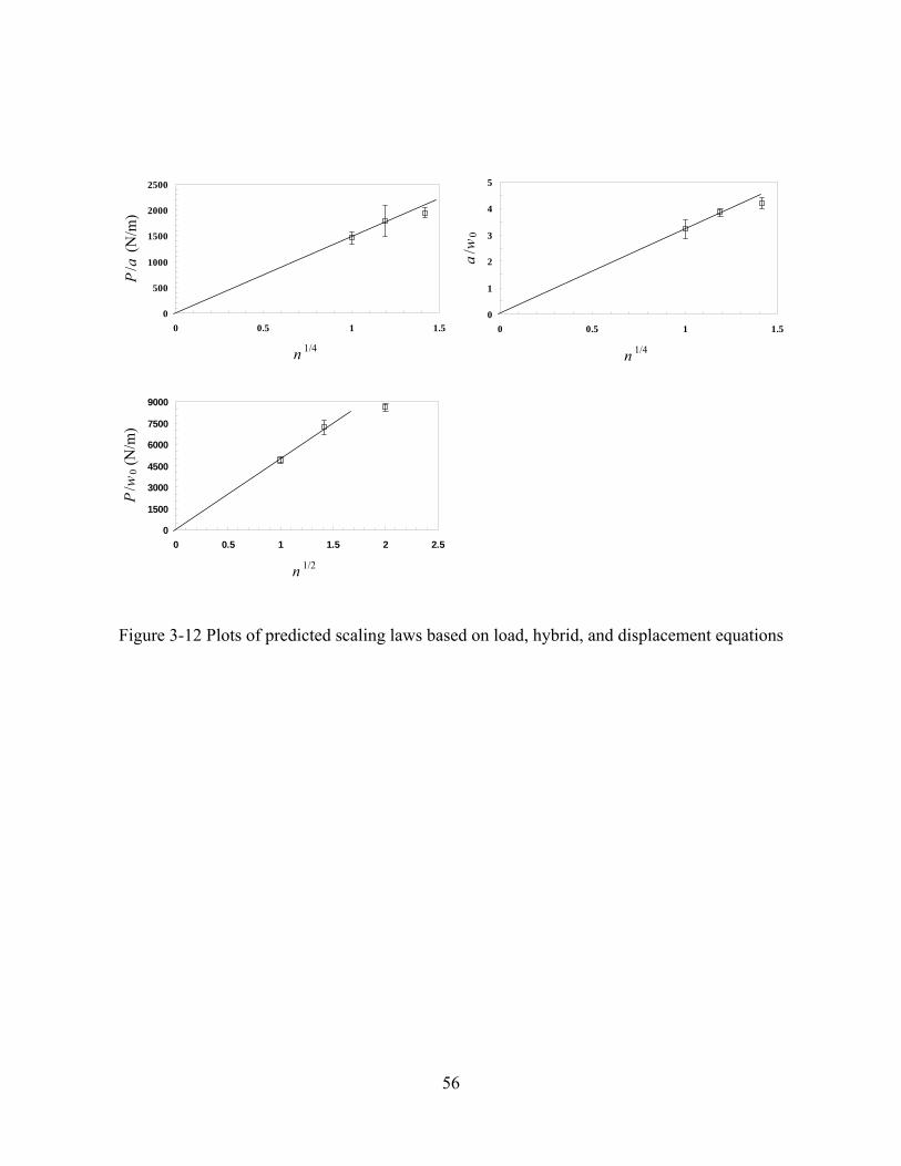
56

0

500

1000

1500

2000

2500

0 0.5 1 1.5

n 1/4

P/a

(N/m

)

0

1

2

3

4

5

0 0.5 1 1.5

n 1/4

a/w

0

0

1500

3000

4500

6000

7500

9000

0 0.5 1 1.5 2 2.5

n 1/2

P/w

0 (N

/m)

Figure 3-12 Plots of predicted scaling laws based on load, hybrid, and displacement equations

57

0

2

4

6

8

10

12

0 1 2 3 4w 0 (mm)

a (m

m)

0

2

4

6

8

10

12

0 1 2 3 4w 0 (mm)

P (N

)

Figure 3-13 Load (P) vs. central shaft displacement (w0), and crack length (a) vs. central shaft

displacement curves (w0), for Kapton® PSA tape bonded to Teflon (n = 1)

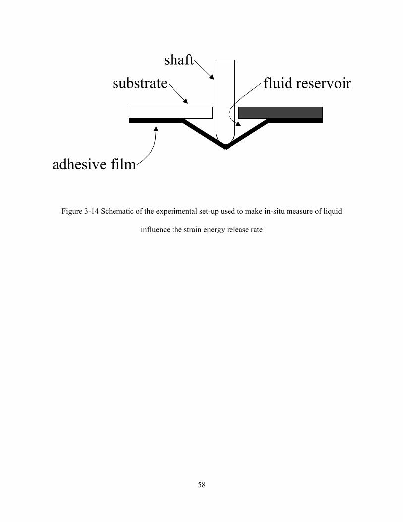
58

adhesive film

shaftsubstrate fluid reservoir

Figure 3-14 Schematic of the experimental set-up used to make in-situ measure of liquid

influence the strain energy release rate

59

0

5

10

15

20

0 1 2 3 4

w 0 (mm)

P (N

)

unexposedwater40%60%80%100%

Figure 3-15 Load (P) vs. central shaft displacement (w0) for various concentrations of methanol

in water (0, 40, 60, 80, 100 wt. %)

60

0

4

8

12

16

20

24

0 1 2 3 4 5

w 03 x 108 (m3)

Pa2 x

104 (m

3 /N)

n = 1n = 2n = 4

Figure 3-16 Linearized plot of equation 7, P a2 vs. w03 for n = 1(□), 2 (о), and 4 (◊)

61

3.3 Moisture Degradation of Epoxy Adhesive Bonds Measured by the

Shaft-Loaded Blister Test

3.3.1 Abstract

In this study, the shaft-loaded blister test was determined to be a relatively simple and convenient

method for characterizing the degradation of adhesive bonds due to moisture exposure. An

experimental sample for this shaft-loaded blister test was developed using reinforcing layers of

Kapton® film. Moreover, the procedure for measuring the blister radius and corresponding

adhesive fracture energy has been greatly simplified by eliminating the need for a video image

recording system. The advantages and disadvantages of the shaft-loaded blister test (SLBT) were

illustrated by studying the effect of relative humidity on the adhesion between a model epoxy

and a quartz substrate. This work has provided further evidence of a critical relative humidity

level for adhesion loss that has been observed in many epoxy systems.

3.3.2 Introduction

3.3.2.1 Critical Relative Humidity for Adhesion Loss

Water is often regarded as the primary agent in the reduction of service life and reliability of

adhesive joints and composites.1-3,101-103 Moisture affects nearly all adhesives performance

because water is ubiquitous in the atmosphere and has a substantial affinity for both organic and

inorganic materials. A class of adhesives that is particularly sensitive to moisture includes the

epoxies. Characteristic of many epoxy – substrate systems is a dramatic loss of adhesion strength

during environmental exposure above a critical relative humidity level.102-111 A typical value of

62

this critical relative humidity level is near 70%, thus limiting the number of applications for these

adhesives.

The mechanism of adhesion loss at a critical relative humidity is the subject of much

speculation. The dramatic reduction in adhesion strength has been attributed to both physical and

chemical changes resulting from moisture absorption in either the bulk of the adhesive or at the

interface between the adhesive and substrate. Brewis et al.108 and Cognard et al.111 proposed that

degradation of the interface is the basic cause for loss of adhesion strength. They suggest that

bonds attributable to secondary forces at the interface are broken up by moisture, hydration of

the oxide surface, and/or water condensation due to lowering of the vapor pressure by the

presence of salt impurities at the interface. Lefebvre and coworkers present the most recent and

detailed study of the critical relative humidity for adhesion loss.102,109 In contrast to Brewis et al.

and Cognard et al., Lefebvre and coworkers conclude that the changes in the bulk properties of

the epoxy adhesive are responsible for the observed onset of adhesion loss at a critical relative

humidity. They reported that the solubility, or mass of absorbed water, as a function of relative

humidity increased abruptly at the critical relative humidity. Similar results led Gledhill et al.103

to propose a critical water concentration in the bulk adhesive for adhesion loss to occur.

Furthermore, the work of Lefebvre and coworkers suggests that capillary condensation, water

condensation on water-soluble impurities, and the depression of the glass transition, are not

responsible for the observed adhesion loss. They proposed that inter-chain hydrogen bonds are

broken by absorption of water. Molecular simulations supported their hypothesis that water

displaced the hydrogen bond network. However, results obtained by Karasz and co-workers60

contradict the hypothesis that inter-chain hydrogen bonds are broken by absorption of water.

Using nuclear magnetic resonance, Karasz and co-workers have shown in epoxies based on the

63

diglycidyl ether of bisphenol A (DGEBA) that no disruption of the hydrogen-bonding network

occurs at room temperature in the hydrated epoxy resin.

3.3.2.2 Research Goal

In this research we explore the shaft-loaded blister test (SLBT).64,90,93,112-114 The experiment

utilizes the controlled displacement of a spherically capped shaft driven by a universal testing

machine (UTM) as an alternative to driving blister growth by applying a fluid or gas media

(Figure 3-17). As discussed in Section 3.2.2 the shaft-loaded blister test has a number of

advantages for environmental testing of adhesives. The advantages and disadvantages of the

SLBT will be highlighted by studying the effect of relative humidity on the adhesion between a

model epoxy and a quartz substrate. This work also provides further evidence of a critical

relative humidity level for adhesion loss that is observed in many epoxy systems.

3.3.3 Experimental

3.3.3.1 Materials

The model epoxy system is Epon 862 bisphenol-f resin (Shell Chemical Corporation) mixed with

10 parts hundred resin (phr) of 1,4-butanediol (added to increase the solubility of the curing

agent) and cured with 3 phr of 4-methyl-2-phenylimidazole.115 The model epoxy was cured for

one hour at 130°C. More details can be found in the dissertation of Case.36 The model epoxy was

bonded to a quartz substrate approximately 3.6 x 3.6 cm2 (1.5 x 1.5 inches square) with a 0.8 cm

(0.31”) diameter hole drilled in the center.

64

3.3.3.2 Blister Test Specimen Preparation

The quartz substrates were boiled in 98 M sulfuric acid for one hour at approximately 150°C to

remove any organic contaminants on the surface. The substrates were then rinsed in deionized

water to remove any trace of sulfuric acid on the surface. A pre-crack was fabricated by placing a

3/8” diameter piece of Kapton® PSA tape (acrylic PSA) over the hole in the center of the quartz

substrate. The Kapton® PSA tape consists of a 25 micron (1 mil) thick Kapton® backing and a

37.5 micron (1.5 mil) thick acrylic pressure sensitive adhesive. The Kapton® PSA tape also

provided additional mechanical reinforcement to the thin epoxy film at the highly stresses

contact area between the coating and shaft-tip. The un-cured model epoxy was coated on to the

quartz substrate. A 50 micron (2 mil) thick piece of Kapton® film was then placed on top of the

epoxy coating. The Kapton® film acts as a mechanical reinforcing layer for the epoxy coating.

The resulting adhesive coating is therefore a composite of the model epoxy, Kapton® PSA tape

and Kapton® film. A schematic of the test specimen is shown in Figure 3-18. The sample was

then cured in a convection oven. The resulting epoxy film was between 50 and 100 microns (2

and 4 mils) thick. Samples were conditioned at constant relative humidity (8, 29, 42, 71, or 98%)

for 3 days at room temperature; long enough for the adhesive to be saturated. The relative

humidity was controlled using saturated salt solutions.116 After environmental exposure the

samples were immediately tested at room temperature at ambient relative humidity (~50%).

Three samples were tested for each relative humidity.

3.3.3.3 Determination of the Adhesive Fracture Energy

The adhesive fracture energy, G, can be calculated from the relationship between the blister

radius, a, and load, P, using Equation 3-9.90

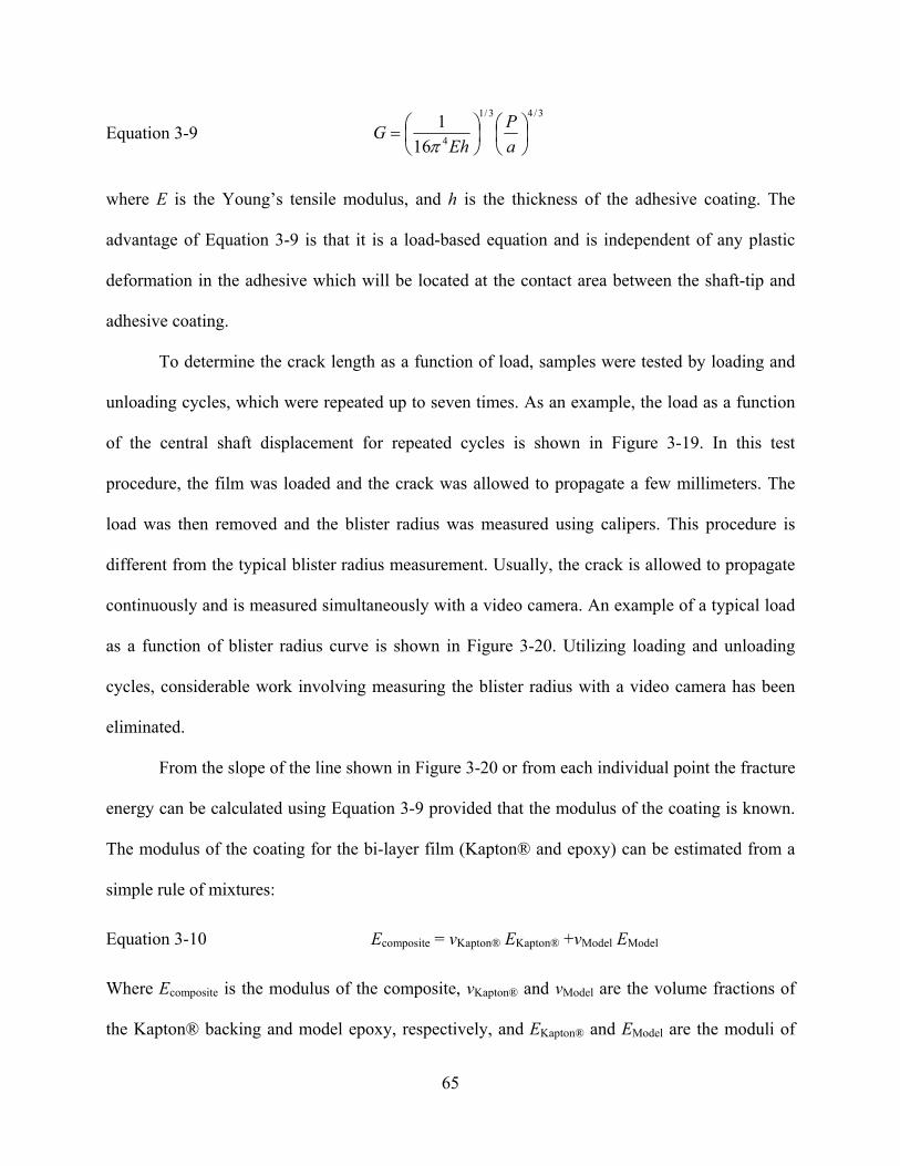
65

Equation 3-9 3/43/1

4161

⎟⎠⎞

⎜⎝⎛

⎟⎠⎞

⎜⎝⎛=

aP

EhG

π

where E is the Young’s tensile modulus, and h is the thickness of the adhesive coating. The

advantage of Equation 3-9 is that it is a load-based equation and is independent of any plastic

deformation in the adhesive which will be located at the contact area between the shaft-tip and

adhesive coating.

To determine the crack length as a function of load, samples were tested by loading and

unloading cycles, which were repeated up to seven times. As an example, the load as a function

of the central shaft displacement for repeated cycles is shown in Figure 3-19. In this test

procedure, the film was loaded and the crack was allowed to propagate a few millimeters. The

load was then removed and the blister radius was measured using calipers. This procedure is

different from the typical blister radius measurement. Usually, the crack is allowed to propagate

continuously and is measured simultaneously with a video camera. An example of a typical load

as a function of blister radius curve is shown in Figure 3-20. Utilizing loading and unloading

cycles, considerable work involving measuring the blister radius with a video camera has been

eliminated.

From the slope of the line shown in Figure 3-20 or from each individual point the fracture

energy can be calculated using Equation 3-9 provided that the modulus of the coating is known.

The modulus of the coating for the bi-layer film (Kapton® and epoxy) can be estimated from a

simple rule of mixtures:

Equation 3-10 Ecomposite = vKapton® EKapton® +vModel EModel

Where Ecomposite is the modulus of the composite, vKapton® and vModel are the volume fractions of

the Kapton® backing and model epoxy, respectively, and EKapton® and EModel are the moduli of

66

the Kapton® backing and model epoxy, respectively. The Kapton® PSA tape is ignored because

it is used only during crack initiation. The modulus of Kapton® is approximately 6 GPa.117 The

modulus of the model epoxy is approximately 2.5 GPa. An additional advantage of Equation 3-9

is that it is fairly insensitive to the value of the modulus of the film. Note the modulus of the film

is lies in the denominator and is raised to the 1/3 power in Equation 3-9. This also reduces any

error introduced by not knowing the change in modulus as a function relative humidity.


The resulting adhesive fracture energies calculated from the load-based equation as a function of

relative humidity are shown in Figure 3-21. At 8, 29, and 42% relative humidity the film ruptures

before debond growth occurs according to Figure 3-21. Also at 71% and 98% relative humidity,

the adhesive interface is degraded sufficiently for crack propagation to occur. The resulting strain

energy release rates were 163 +/- 27 and 111 +/- 27 J/m2 for 71% and 98% relative humidity

respectively. Although the average strain energy release rate of the 98% humidity sample is less

than the 71% as expected, the difference is not substantial if the standard deviation is considered.

These results, which show a dramatic loss of adhesion at 70% relative humidity, are consistent

with a critical relative humidity level for adhesion loss.102-111

Despite the axisymmetric geometry, short saturation time, and relatively simple sample

preparation and test procedure, the shaft-loaded blister test has some shortcomings. As illustrated

in this study, the adhesive film can rupture before debonding can occur. This is attributable to the

large stresses generated within the film near the contact area between the film and shaft tip.

Significant, visible plastic deformation at the contact area may still arise even if film rupture

does not occur and crack propagation takes place. However, if plastic deformation is confined

solely to the center of the blister and not at the crack tip, the fracture mechanics analysis remains

67

valid.64 Plastic deformation and film rupture is a common problem of many adhesive coating test

methods, and is associated with their small load-bearing capacity, their thinness, and their

relatively strong adhesion.79 For these reasons the SLBT is most suitable to environmental

testing where the adhesive interface has been substantially degraded. A decrease in interface

toughness reduces the applied stresses on the adhesive coating during the fracture process.

Utilizing a higher strength material for the backing, such as a metal, could provide enough

reinforcement to produce crack growth at lower values of relative humidity, rather than film

rupture. An alternative means for preventing film rupture would be to reduce the applied load,

and therefore the stress on the film. This strategy is employed in sub-critical fracture experiments

which are discussed in detail in Section 3.4.

3.3.5 Conclusion

The SLBT was demonstrated to be a simple and informative method for characterizing the

degradation of adhesive bonds due to environmental stress. These results illustrate the benefits

and shortcomings of the SLBT, suggesting that this test method is most suitable to environmental

testing of specimens where the adhesive fracture energy has been substantially reduced.

Moreover, this study has also provided an additional example of a critical relative humidity for

adhesion loss which has been previously observed in many epoxy systems.

68

3.3.6 Figures

P

w0

2a

hadhesive film

shaftsubstrate

P

w0

2a

hadhesive film

shaftsubstrate

Figure 3-17.Schematic of the shaft-loaded blister test

substrate

Model epoxy (50-100 µm)

Kapton® film (50 µm)

Kapton® PSA pre-crack P

Figure 3-18 Schematic of shaft-loaded blister test specimen

69

-20

0

20

40

60

80

100

120

0 1 2 3 4 5

w 0 (mm)

P (N

)

Figure 3-19 Successive load as a function of central shaft displacement curves for 98% relative

humidity. The filled in symbols are the loading curves and the unfilled symbols are the unloading

curves.

70

y = 6.6518xR2 = 0.9484

0

20

40

60

80

100

120

0 2 4 6 8 10 12 14 16 18

a (mm)

P (N

)

Figure 3-20. Load vs. blister radius for 98% relative humidity

0

50

100

150

200

250

0 20 40 60 80 100

relative humidity (%)

G (J

/m2 )

film

rupt

ure

film

rupt

ure

film

rupt

ure

0

50

100

150

200

250

0 20 40 60 80 100

relative humidity (%)

G (J

/m2 )

film

rupt

ure

film

rupt

ure

film

rupt

ure

Figure 3-21. Summary of strain energy release rates G (J/m2) vs. relative humidity for critical

SLBT

71

3.4 Environmental Studies of Adhesive Bonds Using the Sub-critical

Shaft-Loaded Blister Test

3.4.1 Abstract

The shaft-loaded blister test has been adopted for sub-critical fracture testing. Two different

epoxy adhesives and environments were investigated. In both cases, the epoxy adhesive was

bonded to a silicon wafer which had a silicon oxide surface. The adhesion of a model epoxy as a

function of relative humidity (42, 71, and 98%) at room temperature was investigated. In

addition, the sub-critical fracture behavior of a commercial filled epoxy, designated as L4, and

exposed to water as function of temperature (60, 70, and 80°C), was also investigated. These

results were correlated to the bulk (non-bonded) adhesive diffusion behavior. This research

suggests that the constant-load sub-critical shaft-loaded blister test is a new and valuable

technique for studying the effects of the environmental degradation on adhesive joints and

coatings. Given the great difficulty in testing thin, strongly adhered coatings and films, this

technique is particularly attractive.

3.4.2 Introduction

3.4.2.1 Sub-Critical Adhesion Testing

Sub-critical adhesion testing is of practical interest to engineers because it explores adhesive

debonding in a range of crack velocities and applied strain energy release rates, G, which are

significantly less than required for catastrophic failure. Sub-critical adhesion testing therefore

more closely resembles the failures observed in the actual application or service of the adhesive.

In these more realistic situations, degradation and failure takes place over long periods of time.

72

In such cases, crack growth can be driven by small applied loads generated by residual stresses,

thermomechanical cycling, and mechanical or vibrational loading.8 Furthermore, sub-critical

testing reduces the ambiguity associated with the measured adhesion energy dependence in crack

velocity, which is associated with viscoelastic effects at the crack tip.

Sub-critical adhesion measurements can be carried out at any temperature and in the

presence or absence of moisture or other environmental fluid. The results are typically presented

in the form of the average crack velocity, v (da/dt) (m/s), as a function of the applied strain

energy release rate (G) or crack driving energy (J/m2). A schematic of a typical v-G curve is

shown in Figure 3-22 (taken from Gurumurthy et al 118). When comparing different

environmental conditions and adhesive systems at a constant velocity, the applied crack driving

energy decreases as the aggressiveness of the environment or chemical activity increases. Figure

3-22 illustrates three regions typically found in a v-G curve, where changes in slope indicate a

change in the rate limiting step for crack advancement.8,119,120 Region III is associated with

critical fracture events and for classic fracture of bulk glasses is independent of the environment.

Region II depends strongly on the environment, little on the crack driving energy, and is

characteristic of fracture where diffusion of the penetrant or environmental fluid to the crack tip

is the rate limiting step to crack advance. Region I is characteristic of low crack velocities and

low applied crack driving energies. For bulk fracture of glasses in Region I, crack growth was

found to be controlled by bond rupture and healing, the ratio of the two governed by the crack

driving energy.121 Furthermore, the crack velocity in Region I is also controlled by the stress-

activated chemical reaction of the penetrant with the bonds at the crack tip.118 At crack velocities

below Region I there exists a threshold value of crack driving energy, GTh, below which no crack

propagation is observed.

73

The v-G curve can adopt several different shapes that are characteristic of the mechanism

of interfacial degradation. Lane et al. observed two characteristic shapes of the v-G curve as the

temperature is increased or as the chemical activity increases, shown in Figure 3-23 121. In the

first case (left graph of Figure 3-23), as the chemical activity is increased, GTh and region II shift

to smaller applied crack driving energies, which Lane et al attribute to a stress-dependent

chemical reaction at the crack debond tip. In the second case (right graph of Figure 3-23), as the

chemical activity is increased the plateau region (region II and corresponding value of v*)

increases and a decrease in the GTh (region I) is not observed. Lane et al indicate that this is

consistent with a steric hindrance mechanism where the crack tip is less than a size of the

penetrant species.

Gurumurthy et al. 118 observed for an epoxy-polyimide interface, as the moisture content

was kept constant and the temperature increased, there was an decrease in both v* and GTh,

which is consistent with a stress and temperature dependent chemical reaction at the crack tip.

Although not shown, alternatively, the v-G curve may also take on the shape of a backwards

letter “C” where the applied crack driving energy goes through a maximum. This behavior is

attributable to viscoelastic effects.

Sub-critical fracture testing can be used to predict the durability of adhesive joints.

Curley et al made theoretical predictions of the fatigue lifetime of adhesive joints based on

mechanical fatigue data.122 Fatigue data measures the rate of crack growth per cycle (da/dN),

rather than rate of growth per second (da/dt), as a function of crack driving energy. The

approaches developed in fatigue (da/dN) can therefore be extended to v-G experiments (da/dt).

In the approach of Curley et al, lifetime predictions were made by modeling the (da/dN) vs. G

74

curve and then calculating the number of cycles until failure based on an initial flaw size and the

applied stress in the joint.

Traditionally, sub-critical fracture tests specimens have been the laminated beam type

where the adhesive is bonded to rectangular rigid adherends. Examples of the laminated beam

type experiments are the double cleavage drilled compression specimen123, four-point flexure

samples124, double cantilever beam wedge test106, and the asymmetric double cantilever beam

test118. The advantages of laminated beam type specimens are: 1) the adhesive is loaded

elastically away from the crack tip, 2) high strain energy release rates are obtainable, 3) the

fracture mechanics models are well understood, and 4) the specimens are often self-loading. For

the double cantilever beam wedge test, the strain energy release rate decreases as a function of

1/a4 yielding a wide range of values of G which can rapidly approach a threshold value. The

disadvantages of all these tests are that they may require sophisticated experimental set-up to

measure the crack length (video camera, acoustic methods, or electrical). Also the time for fluid

saturation of the adhesive may be long because the adhesive is sandwiched between two

impermeable substrates and only edge diffusion into the adhesive may occur.

With respect to the laminated beam type specimens, the advantages of the shaft-loaded

blister test is that the time to saturation is reduced considerably because it is an open face coating

allowing diffusion through the top of the coating rather than edge diffusion. In addition, the

specimen geometry is axisymmetric, which reduces any misleading edge effects caused by

degradation of the interface away from the crack tip. The disadvantages of the shaft-loaded

blister test are that the facture mechanics models have not been studied as extensively as the

laminated beam specimens; and, like most coatings tests, the value of the strain energy release

rates is limited by the film’s mechanical strength. In the case where the film strength is low or if

75

the intrinsic interfacial toughness is high, film rupture can occur, as was observed in the previous

study. Furthermore, the strain energy release rate decreases as a function of 1/a1/3 yielding a

narrow range of values of G that slowly approach a threshold value. Several other disadvantages

exist which we will discuss later.

3.4.2.2 Residual Stress Effects in Critical and Sub-Critical Experiments

Residual stresses can affect the fracture energy of an adhesive if, during debonding, these

stresses change.125 For the peel test and blister test tensile residual stresses reduce the energy

release rate. Conversely, compressive stresses increase the energy release rate. Note that for dry

polymeric adhesives bonded to low coefficient of thermal expansion silicon substrates, these

stresses are tensile. However, due to exposure to elevated temperatures and the absorption of

water, the state of stress in the SLBT specimens is unknown. Allen and Senturia have pointed out

that the energy balance for a blister test does not need to consider residual stress (tensile),

because as long as the edges of the film are attached to the substrate the residual stresses are not

relieved.82 This is also the general case for thin-layer laminated beam specimens, where the

adhesive remains adhered and the strain energy stored in the layer due to residual stress is not

released.126 Furthermore, Allen and Senturia note that in the pressurized blister test at large

pressures the effects of residual stress are overwhelmed by the stresses generated in the film

during testing. However, in the pressurized blister test the residual stress effects the load

deflection behavior. Thus, when utilizing the critical debond pressure; the value of G was less

than expected because of the extra contribution to debonding by residual stresses. Wan and

coworkers studied the load-deflection behavior of the blister test and provide a comprehensive

list of existing work on residual stresses in blister tests.127

76

3.4.3 Experimental

3.4.3.1 Materials

3.4.3.1.1 L4 commercial filled epoxy

L4 is a commercial, filled (21% by weight) epoxy adhesive manufactured by Loctite and

obtained from Hewlett-Packard Co. The L4 epoxy is cured at 140°C for thirty minutes. The glass

transition temperature is 110°C. The modulus is approximately 4 GPa. Details of the material

properties can be found elsewhere.36 A coating thickness on average of 100 +/- 20 microns was

used for the L4 specimens. Distilled water at temperatures of 60, 70, and 80°C was used as the

environmental fluid. Mass uptake experiments were performed also at 60, 70, and 80°C.

3.4.3.1.2 Model Epoxy and Relative Humidity

A description of the model epoxy adhesive can be found in Section 3.3.3.1. Details of the model

epoxy can also be found in the work of Case and Ward.36,115 coating thickness on average of 75

+/- 25 microns was used for the model epoxy specimens. The entire SLBT specimen was paced

in a large glass vessel and conditioned at constant relative humidity (42, 71, or 98%) at room

temperature. The relative humidity was controlled using saturated salt solutions.116

3.4.3.1.3 Silicon Wafer Substrate

The substrate used in this study was a 152.4 mm (6” inch) diameter silicon wafer with a 10 nm

thick thermally grown layer of silicon oxide. These wafers were supplied by the Hewlett-Packard

Comapny.

77

3.4.3.2 Sample Preparation of Constant Load Sub-Critical SLBT Specimens

Two types of self-loaded SLBT specimens were used in this study. Specimens were self-loaded

by suspending a known mass from the center of the blister. The first type of specimen was used

in the model epoxy study where the specimen was completely immersed in the humid

environment. The second type of specimen was used in the L4 adhesive study. Although the

sample must also be self loaded, the sample is not completely immersed in the fluid

environment. In this case, the fluid is confined solely in the fluid reservoir formed by the

adhesive and substrate (see Figure 3-24).

3.4.3.2.1 Preparation of Adhesive Coating and Substrate

A hole approximately 12.5 mm in diameter is fabricated in the center of the silicon wafer using a

diamond coated drill bit and a Dremel® tool. Extreme care must be taken when drilling the

brittle wafers. The wafer is then rinsed with IPA and blown dry with ultra-high purity nitrogen

gas. The hole in the wafer is then covered with a 19 mm (3/4 inch) diameter piece of Kapton®

PSA tape (acrylic based adhesive). The Kapton® tape serves two purposes: 1) it forms a pre-

crack for the crack to initiate and 2) acts as an additional mechanical reinforcement layer for the

adhesive in the vicinity where the load is suspended. The wafer is coated with epoxy adhesive

using a pneumatically driven doctor blade. A 152.4 x 152.4 mm (6” x 6”) square piece of

Kapton® (50 microns thick) is carefully applied on the wafer to avoid disrupting the adhesive

and the formation of air bubbles. The coated wafer (with Kapton®) is then cured and removed

from the oven and is placed in a dessicator to slowly cool down (approximately 30 minutes).

78

3.4.3.2.2 Preparation of Model Epoxy Self-Loaded SLBT Specimen (No Self-Contained Fluid

Environment)

To develop a sub-critical blister test specimen the sample must be self-loading. Also, the

integrity of the thin adhesive coating must be maintained and the sample must be exposed to the

fluid in this experiment. To fabricate a simple self-loading constant load SLBT specimen a hole

is punched in the coating that can accommodate a 2.54 mm (or 4/40”) stainless steel machine

screw. The machine screw acts as the fastener from which to suspend the load (via a flexible

copper wire). The punched hole containing the screw is sealed with a room temperature cure

epoxy (Devcon 2-ton Epoxy). A photograph of this type of self loading specimen with the

applied adhesive, Kapton® reinforcement layer, and attached screw is shown in Figure 3-26. The

entire specimen with the suspended weight was then set in the environmental chamber. The

entire adhesive is exposed to the moist environment during testing and is saturated.

3.4.3.2.3 Preparation of L4 Self-Loading SLBT Specimen with Self-Contained Fluid

Environment

The L4 adhesive SLBT specimens require a self-contained fluid environment shown

schematically in Figure 3-25. The self-contained environment is necessary to minimize the space

occupied by the wafers in the convection oven. The self-loaded sample described in the prior

section can be modified using a pair of o-rings, a Teflon® sheet, a steel sheet and some clamps.

As shown in Figure 3-25 the fluid reservoir is formed by the blister and substrate and sealed with

a rigid top-piece sheet of steel or aluminum and two silicon rubber o-rings: a center (smaller) o-

ring and an outer (larger) o-ring. Between the o-rings and the steel is a thin piece of Teflon®

film which acts as a barrier and curbs any chemical reaction which may occur between the metal

79

sheet and water. Pressure on the o-ring is achieved using Kant-twist® c-clamps. Given the

brittleness of the wafer it is important to use delicate c-clamps to avoid damaging the wafer. The

o-rings and Teflon® are cleaned with isopropyl alcohol to provide an excellent seal. To ensure

that there is no difference in pressure between the blister and outside environment (a vacuum), a

small vent is utilized. The vent is a syringe needle that has been inserted into the outer o-ring

creating a passage for gas to travel from the fluid reservoir to the outside atmosphere. The center

(smaller) o-ring has a large cut to allow for the free passage of water and gas inside the fluid

reservoir. A significant disadvantage of this experimental set-up is the inevitable evaporation and

small coating thickness that facilitates fluid loss by permeation. Because of these factors, it is

difficult to test volatile fluids such as the ink vehicles supplied by Hewlett-Packard.

3.4.3.3 General Procedure and Analysis for Sub-Critical Blister Testing

3.4.3.3.1 Model Epoxy

As mentioned previously, the loaded model epoxy specimens are placed entirely in a constant

relative humidity environment. Samples are removed periodically to measure the blister radius as

a function of time. The blister radius is measured with calipers.

3.4.3.3.2 L4 Adhesive

The reservoir is filled with distilled water up to the top level of the o-rings and sealed up. The

entire set up can be then placed in the convection oven. A photograph of the L4 specimens in a

convection oven is shown in Figure 3-27. Samples are removed periodically to measure the

blister radius as a function of time. After measuring the crack length, the fluid reservoir is topped

off with water.

80

3.4.3.3.3 Analysis

Using the load-based equation (Equation 3-11), from the load, P, and blister radius, a, the crack

driving energy, G, can be calculated.

Equation 3-11 3/43/1

4161

⎟⎠⎞

⎜⎝⎛

⎟⎠⎞

⎜⎝⎛=

aP

EhG

π

The blister radius is measured periodically with a micrometer as function of time. Two or three

micrometer measurements are utilized to calculate the average blister radius. These were used to

determine the average crack velocity v or (da/dt). The crack velocity is expressed in units of m/s.

The modulus of the coating for the bi-layer film (Kapton® and epoxy adhesive) can be

estimated from a simple rule of mixtures:

Equation 3-12 Ecomposite = vKapton® EKapton® +vEpoxy EEpoxy

Where Ecomposite is the modulus of the composite, vKapton® and vEpoxy are the volume fractions of

the Kapton® backing and epoxy, respectively, and EKapton® and EEpoxy are the moduli of the

Kapton® backing and epoxy, respectively. The modulus of Kapton® is approximately 6 GPa.117

Because the film tensile rigidity (Eh) is in the denominator of equation Equation 3-11 and is also

raised to the 1/3 power, the expression for the crack driving energy is relatively insensitive to the

value of (Eh). The advantage is that the value of G is insensitive to the numerical values of the

modulus and thickness which are a function of the temperature and fluid content.

3.4.3.4 Mass Uptake Experiments

Diffusion coefficients, D, and equilibrium moisture saturation level, M∞, of water in the L4

adhesive as a function of temperature were obtained by traditional mass uptake experiments.

Mass uptake specimens had dimensions of 10 mm x 50 mm x 0.5 mm and were cured in silicone

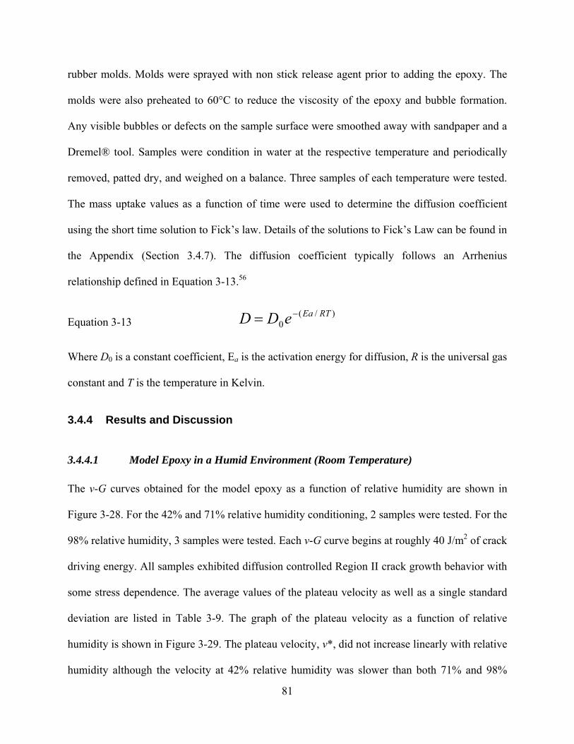
81

rubber molds. Molds were sprayed with non stick release agent prior to adding the epoxy. The

molds were also preheated to 60°C to reduce the viscosity of the epoxy and bubble formation.

Any visible bubbles or defects on the sample surface were smoothed away with sandpaper and a

Dremel® tool. Samples were condition in water at the respective temperature and periodically

removed, patted dry, and weighed on a balance. Three samples of each temperature were tested.

The mass uptake values as a function of time were used to determine the diffusion coefficient

using the short time solution to Fick’s law. Details of the solutions to Fick’s Law can be found in

the Appendix (Section 3.4.7). The diffusion coefficient typically follows an Arrhenius

relationship defined in Equation 3-13.56

Equation 3-13 )/(

0RTEaeDD −=

Where D0 is a constant coefficient, Ea is the activation energy for diffusion, R is the universal gas

constant and T is the temperature in Kelvin.


3.4.4.1 Model Epoxy in a Humid Environment (Room Temperature)

The v-G curves obtained for the model epoxy as a function of relative humidity are shown in

Figure 3-28. For the 42% and 71% relative humidity conditioning, 2 samples were tested. For the

98% relative humidity, 3 samples were tested. Each v-G curve begins at roughly 40 J/m2 of crack

driving energy. All samples exhibited diffusion controlled Region II crack growth behavior with

some stress dependence. The average values of the plateau velocity as well as a single standard

deviation are listed in Table 3-9. The graph of the plateau velocity as a function of relative

humidity is shown in Figure 3-29. The plateau velocity, v*, did not increase linearly with relative

humidity although the velocity at 42% relative humidity was slower than both 71% and 98%

82

relative humidity. This is in contrast to model proposed by Wiederhorn128 for Region II crack

growth of glass in moist air. Weiderhorn showed that the plateau velocity is linearly dependent

on the relative humidity which agrees well with what has been observed in the literature124,129.

Table 3-9 The plateau velocity, v*, as a function of relative humidity for the model epoxy-silicon

oxide adhesive system

42 % rh 71% rh 98% rh

Average v* (m/s) 1.6 x 10-9 3.6 x 10-9 3.3 x 10-9

Standard Deviation 7.2 x 10-10 3.0 x 10-10 1.9 x 10-9

The average and single standard deviation of the threshold values of G as function of

relative humidity are listed in Table 3-10. The results in Table 3-10 show that the threshold

values of G are similar for 71% and 98% relative humidity. Moreover, the threshold value of G

for 42% relative humidity is significantly higher than either the 71 or 98% relative humidity

cases. The independence of the threshold value of G on relative humidity was unexpected. The

threshold value of G is theoretically dependent on the partial pressure of water and has been

confirmed experimentally.124,129 The sub-critical SLBT may not be sensitive enough to detect

any significant differences between the 71% and 98% relative humidity conditioning. This

postulate is plausible, given the similarity between the values of G measured by the traditional

SLBT method (Section 3.3) and the experimental uncertainty. The experimental uncertainty is

discussed in the next section. In addition, condensation at the crack tip would negate any relative

humidity differences and would also lead to similar threshold value of G observed for 71% and

98% relative humidity.

83

Table 3-10 The threshold value of G as function of relative humidity for the model epoxy-silicon

oxide adhesive system.

42 % rh 71% rh 98% rh

Average GTh (J/m2) 25.2 10.2 11.5

Standard Deviation 4.9 2.1 2.6

Error is introduced in the calculation of the values of ,G, and crack velocity ,v, that are

associated with measuring the blister radius, a. The error associated with measuring the blister

radius with the micrometer is approximately ± 0.2 – 0.3 millimeters. In addition, the blister may

not be entirely symmetric. In the most extreme cases, the difference between two measurements

of the same blister radius was 0.5 mm. The error attributable to the blister radius measurement

depends on the magnitude of the value of G and crack velocity. Values of G that ranged between

20-50 J/m2 had a small error ranging from ± 1-2 J/m2. Values of G that ranged between 1 - 20

J/m2 had an error between ± 0.1 – 0.5 J/m2. Crack velocities on the order of 10-8 and 10-9 m/s had

errors on the order of a ± 10%, which was much less than the inherent scatter of the experiment.

The error was significant for crack velocities approaching 10-10 m/s or less; however, at these

crack velocities the experimental limit of the measurement is being rapidly approached and these

cracks appear to arrest.

The sub-critical results of the model epoxy-silicon oxide wafer adhesive system can be

compared to the results of the model epoxy-quartz adhesive system (Section 3.3). The quartz

substrate and silicon wafer substrate are expected to have similar surfaces given that they both

are silicon oxide. In the model epoxy-quartz experiments, evidence was presented that suggested

there was a critical level of relative humidity where adhesion loss occurred. At a relative

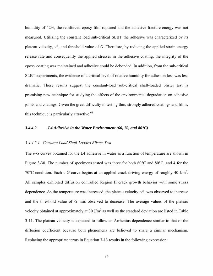
84

humidity of 42%, the reinforced epoxy film ruptured and the adhesive fracture energy was not

measured. Utilizing the constant load sub-critical SLBT the adhesive was characterized by its

plateau velocity, v*, and threshold value of G. Therefore, by reducing the applied strain energy

release rate and consequently the applied stresses in the adhesive coating, the integrity of the

epoxy coating was maintained and adhesive could be debonded. In addition, from the sub-critical

SLBT experiments, the evidence of a critical level of relative humidity for adhesion loss was less

dramatic. These results suggest the constant-load sub-critical shaft-loaded blister test is

promising new technique for studying the effects of the environmental degradation on adhesive

joints and coatings. Given the great difficulty in testing thin, strongly adhered coatings and films,

this technique is particularly attractive.65

3.4.4.2 L4 Adhesive in the Water Environment (60, 70, and 80°C)

3.4.4.2.1 Constant Load Shaft-Loaded Blister Test

The v-G curves obtained for the L4 adhesive in water as a function of temperature are shown in

Figure 3-30. The number of specimens tested was three for both 60°C and 80°C, and 4 for the

70°C condition. Each v-G curve begins at an applied crack driving energy of roughly 40 J/m2.

All samples exhibited diffusion controlled Region II crack growth behavior with some stress

dependence. As the temperature was increased, the plateau velocity, v*, was observed to increase

and the threshold value of G was observed to decrease. The average values of the plateau

velocity obtained at approximately at 30 J/m2 as well as the standard deviation are listed in Table

3-11. The plateau velocity is expected to follow an Arrhenius dependence similar to that of the

diffusion coefficient because both phenomena are believed to share a similar mechanism.

Replacing the appropriate terms in Equation 3-13 results in the following expression:

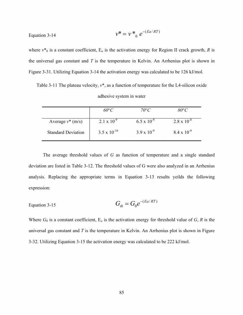
85

Equation 3-14 )/(

0** RTEaevv −=

where v*0 is a constant coefficient, Ea is the activation energy for Region II crack growth, R is

the universal gas constant and T is the temperature in Kelvin. An Arrhenius plot is shown in

Figure 3-31. Utilizing Equation 3-14 the activation energy was calculated to be 126 kJ/mol.

Table 3-11 The plateau velocity, v*, as a function of temperature for the L4-silicon oxide

adhesive system in water

60°C 70°C 80°C

Average v* (m/s) 2.1 x 10-9 6.5 x 10-9 2.8 x 10-8


The average threshold values of G as function of temperature and a single standard

deviation are listed in Table 3-12. The threshold values of G were also analyzed in an Arrhenius

analysis. Replacing the appropriate terms in Equation 3-13 results yeilds the following

expression:

Equation 3-15 )/(

0RTEa

th eGG −=

Where G0 is a constant coefficient, Ea is the activation energy for threshold value of G, R is the

universal gas constant and T is the temperature in Kelvin. An Arrhenius plot is shown in Figure

3-32. Utilizing Equation 3-15 the activation energy was calculated to be 222 kJ/mol.

86

Table 3-12 The threshold value of G as function of temperature for the L4 epoxy-silicon oxide

adhesive system exposed to water.

60°C 70°C 80°C

Average GTh (J/m2) 19.5 6 0.2

Standard Deviation 1 1 0.1

3.4.4.2.2 Bulk Diffusion Measurement

The diffusion coefficient, D, and equilibrium moisture saturation level, Msat, of water in the bulk

(non-bonded) L4 adhesive as a function of temperature were obtained by mass uptake

experiments. The temperature dependence of the absorption behavior and the diffusion

controlled Region II behavior of the sub-critical SLBT were compared. These results were also

used to predict the moisture content of L4 adhesive joints and coatings used in the impedance

studies. A graph of the normalized percent moisture uptake as a function of the square root of

time (seconds) normalized by the sample thickness for each temperature is shown Figure 3-33.

Only the initial Fickian stage of diffusion is shown in Figure 3-33. The L4 epoxy exhibits two-

stage or non-Fickian diffusion at all tested temperatures, which is characteristic of many epoxy

systems. The graph of the percent moisture uptake as a function of the square root of time

(seconds) normalized by the sample thickness for each temperature is shown in Figure 3-34.

Figure 3-34 illustrates the non-Fickian behavior observed for all three temperatures. The

diffusion coefficient and equilibrium moisture saturation level as a function of temperature are

listed in Table 3-13 and Table 3-14 respectively. As the temperature is increased, the diffusivity

87

increases. The equilibrium moisture saturation level appears to be independent of the

temperature.

Table 3-13 The average diffusion coefficient, D, of water in the L4 epoxy as a function of

temperature. A single standard deviation is also listed.

60°C 70°C 80°C

Average D (cm2/s) 1.3 x 10-8 2.2 x 10-8 3.8 x 10-8


Table 3-14 The average equilibrium moisture saturation level, M∞, of water in the L4 epoxy as a

function of temperature. A single standard deviation is also listed.

60°C 70°C 80°C

Average %M∞ (grams) 2.5 2.6 2.5

Standard Deviation 0.1 0.1 0.1

3.4.4.2.3 Discussion of Activation Energies

The Arrhenius plot of the diffusion coefficient is shown in Figure 3-35. The calculated activation

energy for the diffusion process is 53 J/mol. This value falls in the expected range of activation

energies for moisture diffusion into epoxy adhesives, which typically range between 30 – 50

kJ/mol59. The activation energies for the plateau velocity and threshold value of G are 126 J/mol

and 222 J/mol, respectively. These values are an order of magnitude greater than the activation

energy for diffusion. This is not unexpected given that both the plateau velocity and threshold

value of G depend not only on the rate of transport of fluid to the crack tip but also on the

88

applied stress. The dependence of the Region II crack velocity and threshold value of G on the

applied stress is evident from the slope of the v-G curve. The idea that rate limiting step for the

Region II crack growth that is not diffusion controlled is supported by the sub-critical SLBT

relative humidity study of the model epoxy as well as and preliminary results in 2003 from Singh

and Dillard at Virginia Tech.

In the model epoxy adhesive SLBT study, the specimens were stored long term in the

moist environment and are therefore entirely saturated with moisture. As a consequence,

moisture was always present near the crack tip. Effectively, the process of diffusion of moisture

to the crack tip has been “turned off”. Nevertheless, Region II diffusion controlled crack growth

was observed despite the fact the adhesive was saturated. This suggests that Region II behavior is

not solely dependent on diffusion, but depends also on stress. Similar, unpublished, results were

obtained by Singh and Dillard (Virginia Tech, 2003) who studied sub-critical fracture of the L4

epoxy in fluid environments using the wedge test. They observed similar v-G curves between

samples that were saturated with fluid before testing and samples that were not preconditioned.

.

3.4.5 Summary

The shaft-loaded blister test was adopted for sub-critical fracture testing by applying a self-

loading mechanism whereby a mass is suspended from the center of the inverted blister. The

adhesion of the model epoxy to silicon oxide as function of relative humidity (42, 71, and 98%)

at room temperature was characterized. Notably, the adhesion at low humidity (42%) was

measured, where the traditional SLBT was unsatisfactory. An Arrhenius analysis of the L4

epoxy and the sub-critical fracture behavior of the saturated model epoxy adhesive suggest that

the Region II behavior is not solely dependent on the diffusion of fluid to the crack tip. These

89

results suggest the constant-load sub-critical shaft-loaded blister test is promising as a new

technique for studying the effects of the environmental degradation on adhesive joints and

coatings. In particular, the application of the sub-critical SLBT technique for testing adhesive

coatings is promising given their typical experimental difficulties.

90

3.4.6 Figures

Log

Cra

ck V

eloc

ity, v

(m/s

)

Crack Driving Energy, G (J/m2)

I

II

III

GTh

Log

Cra

ck V

eloc

ity, v

(m/s

)


I

II

III

Log

Cra

ck V

eloc

ity, v

(m/s

)


I

II

III

GTh

Figure 3-22. Schematic of v-G curve illustrating three region of crack growth

Increasedchemical activity

Cra

ck V

eloc

ity, v

(m/s

)



Cra

ck V

eloc

ity, v

(m/s

)


Cra

ck V

eloc

ity, v

(m/s

)


Increasedchemical activityC

rack

Vel

ocity

, v(m

/s)



Figure 3-23. Schematic of typical behavior as the chemical activity changes.

91

Fluid reservoirFluid reservoir

Figure 3-24 Schematic of the fluid reservoir formed between the adhesive membrane and

substrate.

weight

Vent

Fluid reservoirP P

P P

4/40” screw

wire

Nut and washer

Epoxy sealant

Steel squarelined withTeflon®

wafer substrate Adhesive film

O-ring

weight

Vent

Fluid reservoirP P

P P

4/40” screw

wire

Nut and washer

Epoxy sealant

Steel squarelined withTeflon®

wafer substrate Adhesive film

O-ring

Figure 3-25 Schematic of the sub-critical shaft-loaded blister test specimen.

92

Figure 3-26 Photograph of L4 adhesive blister specimen.

93

Figure 3-27 Photograph of sub-critical shaft-loaded blister test specimens in oven environment.

94

Figure 3-28 SLBT crack velocity (m/s) as a function of crack driving energy, G, (J/m2) and

relative humidity (25°C). The adhesive is the model epoxy.

1.0E-09

1.0E-08

0% 20% 40% 60% 80% 100% 120%

relative humidity

plat

eau

velo

city

, v*

(m/s)

Figure 3-29 The crack velocity of Region II as a function of relative humidity (25°C). The

adhesive is the model epoxy.

1.E-11

1.E-10

1.E-09

1.E-08

1.E-07

1.0

crac

k ve

loci

ty, d

a/d

t (m

/s)

10.0 100.0


42% rh71% rh98% rh

3.0

95

1.E-11

1.E-10

1.E-09

1.E-08

1.E-07

0.1 1.0 10.0 100.0 1000.0

crack driving energy, G (J/m2)

crac

k ve

loci

ty da

/dt

(m/s

) 60°C70°C80°C

Figure 3-30 SLBT crack velocity (m/s) as a function of crack driving energy, G, (J/m2) and

temperature. The environment is water and the adhesive is the L4 epoxy.

96

1.00E-09

1.00E-08

1.00E-07

2.800 2.850 2.900 2.950 3.000 3.050

1000 / T(K)

Log

v* (m

/s)

Figure 3-31 Arrhenius plot of the L4 adhesive plateau velocity exposed to water at 60, 70, and

80°C.

0.1

1

10

100

2.800 2.850 2.900 2.950 3.000 3.050

1000 / T(K)

Log G

(J/m

2 )

Figure 3-32 Arrhenius plot of the L4 adhesive threshold value of G exposed to water at 60, 70,

and 80°C.

97

0

0.2

0.4

0.6

0.8

1

1.2

0 2000 4000 6000 8000 10000

time (seconds)1/2 / thickness (cm)

M /

Meq

60°C70°C80°C

Figure 3-33 The normalized percent mass uptake as a function of the square root of time

(seconds) normalized by the sample thickness for each temperature. The adhesive is the L4

epoxy.

98

0

0.5

1

1.5

2

2.5

3

0 5000 10000 15000 20000

time (seconds)1/2 / thickness (cm)

M % 60°C

70°C80°C

Figure 3-34 The percent mass uptake as a function of the square root of time (seconds)

normalized by the sample thickness and for each temperature. The adhesive is the L4 epoxy.

-8-7.9-7.8-7.7-7.6-7.5-7.4-7.3

2.800 2.850 2.900 2.950 3.000 3.050

1000 / T(K)

Log

D (c

m2 /s

)

Figure 3-35 Arrhenius plot of the temperature dependence of the diffusion coefficient of water in

the L4 epoxy.

99

3.4.7 Appendix: Measuring Diffusion Coefficients

3.4.7.1 Solutions to Fick’s Law of Diffusion

Characteristic of ideal Fickian diffusion is that at short times the initial relative mass uptake is a

linear function of √t and that with time, an equilibrium or final value M∞ is obtained. If indeed

this is the case, there are several approximate solutions to Fick’s law which can be written in

terms of the capacitance of the film and used to solve for the diffusion coefficient and or

concentration (Cp,t)as a function of time t and distance x. For a coating, where the polymer is

insulated on one side, the coating thickness is L.

Utilizing the short time approximation (Mt/M∞ ≤ 0.5), the diffusion coefficient D can be

calculated by equation 10 using the linear portion of the relative mass uptake vs. of √t curve.

Equation 3-16 πtD

LMM 2

=∞

If there is limiting data at short times (M/M∞ ≤ 0.5) then the long time solution may be utilized

(equation 11).

Equation 3-17 2

2

2 48ln1ln

LtD

MM π

π−⎟

⎠⎞

⎜⎝⎛=⎟⎟

⎠

⎞⎜⎜⎝

⎛−

∞

)

In addition, the diffusion coefficient may be calculated by measurement of the half time (t0.5)

where the relative mass fraction is equal to 0.5 then

Equation 3-18 5.0

24*04919.0t

LD =

Furthermore, the time for a material to attain 99.9% of its maximum possible fluid is:130

100

Equation 3-19 D

Ltsat

2467.0 ⋅=

.

101

4 INVESTIGATION OF THE DURABILITY OF ADHESIVE

JOINTS AND COATINGS USING CONSTANT FREQUENCY

IMPEDANCE SPECTROSCOPY

4.1 Introduction

Given the deleterious effects of fluids on adhesion, it is of great interest to know the transport

rate and relative concentration of fluid at an adhesive interface. Utilizing constant frequency

interfacial impedance spectroscopy (IIS) and a novel interdigitated electrode sensor design,

changes in the concentration of absorbed fluid near the interface as a function of exposure time

were correlated to the measured capacitance. These novel IIS sensors measure the impedance of

mapped areas of the sensor defined with respect to the free edge of the coating. Consequently,

these sensors can be used to measure the distribution and transport of fluids at the interface. This

research is divided into the following sections:

1. The design and utility of the IIS sensor are demonstrated by studying the diffusion of

acetone into a pressure sensitive adhesive tape bonded to the sensor.131

2. The capability to measure debonding of an adhesive is demonstrated using a pressure

sensitive adhesive tape exposed to water.

3. The diffusion of an extremely aggressive fluid into a commercial filled epoxy was

studied.

102

4. The diffusion of moisture into UV curable pressure sensitive adhesives was studied.

5. The effects of hygroscopic cycling on the commercial filled epoxy as a function of

fluid environment, surface chemistry, and coating thickness was investigated

6. Sources of signal noise and recommended experimental set-up modifications are

discussed.

103

4.2 Background on Impedance Spectroscopy

Impedance spectroscopy is one of several techniques that belong to a broad class of polymer

characterization methods that are based on measuring a materials response to an electrical

excitation. Impedance spectroscopy, dielectric spectroscopy, microdielectrometry, dielectric

relaxation spectroscopy, and dielectric thermal analysis are all essentially the same technique and

only differ by name and emphasis of observables. These techniques have been used to elucidate

molecular relaxations 132,133, monitor in real time changes in the chemical and physical state in

polymers brought about by crystallization 134 and cure 135, measure fluid diffusion into polymers

136, measure the moisture content of adhesive joints 137,138, and monitor the integrity of the

adhesive joints and coatings 20,138,139.

The impedance Z* or Z(jω), is defined as the total opposition a component offers to the

flow of an alternating current at a given frequency.140 The impedance Z(jω) can be expressed as:

Equation 4-1 Z(jω) = Z′ + jZ″

where Z′ and Z″ are the real and imaginary parts of the impedance, or in-phase and out-of phase

components, respectively. The real part of impedance is equal to the resistance (R), and the

capacitance (C) is related to the imaginary part of the impedance:

Equation 4-2 fC

Zπ21

=′′

Therefore, the impedance is made up of both a capacitive and resistive component. The terms

impedance and capacitance will be used interchangeably in this work.

104

4.2.1 Constant Frequency Impedance Measurements

For qualitative information about the evolution of coating properties as a function of exposure

time to a fluid environment, single or constant frequency impedance measurements can be

utilized.141,142 Because the true coating resistance and capacitance are frequency dependent, more

quantitative results may be obtained by exploring a wide range of frequencies (101 to 106 Hz)

and by fitting the impedance to physically relevant equivalent circuits.143 However, this current

investigation utilizes a single frequency due to the limitations of the testing device. In a constant

frequency experiment, the capacitance and resistance are measured as a function of time of

exposure. The capacitance increases due to increase in the average permittivity of the medium as

fluid is absorbed into the polymer. The resistance decreases due to the ionic or conductive nature

of the absorbed fluid and dissolved ionic species. Alternatively, the impedance of the coating can

be measured before and after exposure to test for the occurrence of irreversible damage.143 This

is the technique employed in the present research to measure the effects of hygroscopic cycling.

For many adhesive coatings, four regions of a graph of the coating capacitance as a

function of exposure time can be distinguished (Figure 4-1).139 Region I corresponds to an

induction period where the fluid must ingress across the thickness of the coating until the fluid

reaches the polymer/electrode interface. At the interface the change in capacitance resulting from

the presence of the fluid can be detected.

In Region II, once the presence of the fluid is detected at the electrode interface, the

concentration of absorbed fluid and capacitance continues to increase. If the adhesive coating

exhibits Fickian diffusion, a linear relationship between the capacitance and t ½ is predicted.

In Region III the polymer is saturated with the fluid. If the adhesive coating exhibits

Fickian diffusion, the values of capacitance and resistance will reach a plateau. If, however, the

105

adhesive coating exhibits non-Fickian diffusion, typical for glassy polymers, the adhesive

coating will exhibit an indefinite uptake of fluid. Under such circumstances, a constant or

equilibrium value of capacitance or resistance will not be observed. For the Fickian case, from

Regions II and III the diffusion coefficient can be obtained using any of several solutions for

Fick’s second law.

Region IV is the final region; there, a rapid rise in capacitance and a rapid decrease in

resistance are observed, corresponding to failure or debonding of the adhesive. The rapid rise or

fall in measured values is attributable to an accumulation of fluid at the interface of the coating

and displacement of the adhesive bonds immediately located next to the electrode interface.

Sekine proposed a method of evaluation based on the changes in the values of resistance of

an adhesive coating.144 The time when the resistance of the adhesive coating suddenly drops is

defined as the breaking time tb. The time when the resistance of the adhesive coating reaches the

value of resistance of the substrate in contact with the fluid is defined as ts. The values of tb and ts

can be used as measures of the apparent lifetime t′ of the adhesive (see Figure 4-2).

4.2.2 The Relationship between Capacitance and Fluid Concentration

Determining the diffusivity of a fluid utilizing capacitance data has been reviewed by Wind and

Lenderink.57 Capacitance data has been used extensively to measure the diffusivity of water in

polymers largely due to the high sensitivity of the polymers dielectric constant to changes in the

volume of absorbed water. The dielectric constant of the coating will change significantly as the

polymer absorbs water because the dielectric constant of polymers is small (ε ~ 3-8) compared

to water (ε ~ 80). The dielectric constant of the wet polymer can be estimated if the water and

polymer are treated as two separate individual phases having appropriate volume fractions. If we

ignore the presence of incorporated air in the polymer and assume the value the dielectric

106

constant of absorbed water is roughly the same as free water, the dielectric constant of the wet

polymer may be described by a rule of mixtures (an effective medium theory):

Equation 4-3 f (εavg) = (1 - φ) f (εcoating) + φ f (εwater)

where f is the function characteristic of the mixing law, εavg is the dielectric constant of the wet

polymer, φ is the volume fraction of absorbed water, εcoating is the dielectric constant of the

coating and εwater is the dielectric constant of water. For a stratified material the following

functions may be appropriate:

parallel to the electric field: f (εavg) = ε

perpendicular to the electric field: f (εavg) = 1 / ε

For the case of a isotropic distribution of water in the polymer, Brasher and Kingsbury proposed

the following empirical mixing laws for polymers absorbing water:145

Brasher and Kingsbury: f (εavg) = log (ε)

More complex models include the Rayleigh function and the effective medium approximation

(EMA).57

The capacitance and permittivity, for an ideal capacitor, are related by the following

expression:

Equation 4-4 ε = C / Q

where Q is a geometric factor. For an ideal parallel plate capacitor, the constant, Q is:

Equation 4-5 Q = ε0 A/d

107

where ε0 is the permittivity of free space, A is the surface area of a single plate, and d is the plate

spacing or dielectric thickness.

Note that the change in permittivity or capacitance is proportional to the change in

volume fraction or concentration of fluid according to the above equations. For water polymer

mixtures, the increase in permittivity and water concentration is proportional to the number of

water dipoles present in the system.146,147

The most widely used empirical function that relates the capacitance to the volume

fraction of water in coatings is that of Brasher and Kingsbury, which reduces to:

Equation 4-6 )80log(

))(log()( coatingC

tC

t =φ

Where:

φ(t): the volume fraction of water at time t

C(t): the measured capacitance of the mixture of the polymer coating and water at time t

Ccoating: the measured capacitance of the dry polymer coating at t = 0

The assumptions of the Brasher-Kingsbury equation (Equation 4-6) are:139

1. The change in capacitance is entirely due to the permeation of water into the film.

2. The water uptake does not cause the coating to swell.

3. The water is distributed homogeneously in the coating.

4. The permittivity of water is constant and equal to 80.

5. No polar solvent is present in the coating.

6. The values of capacitance of the coating can be expressed by Equation 4-4 and

Equation 4-5.

7. The volume fraction penetrated by water remains relatively small.

108

This list is a useful as a general guideline of the assumptions used in the application of any of the

rule of mixtures or effective medium theories.

According to Fodor and Hill, for interdigitated structures the field decays at large

distances (z < L / π), where z is the distance above the sensor surface and L is the line spacing.148

For the IIS sensor electrode geometry (L = 72 microns) the field is expected to exponentially

decay 23 microns above the surface. Despite this relatively large distance, interdigitated

electrodes are regarded to be a local measurement of the capacitance at the surface and therefore

of the concentration of fluid (C) near the surface of the sensor. Furthermore, the capacitance is

not a measurement of the average mass of absorbed fluid (M) in the adhesive. Therefore, in an

approach similar to that utilized by Day et al 136, Equation 2-2 can be expressed in terms of the

capacitance.


⎜⎝⎛ +

⎥⎦

⎤⎢⎣

⎡ +−

+−

−=−− ∑

∞

==

=

Lxn

LtnD

nCCCC

n

n

tf

tt

2)12(cos

4)12(exp

12)1(41

02

22

0

0 πππ

where C t is the permittivity at any time t, Ct=0 is the initial permittivity of the polymer film and

Cf is the permittivity at the surface after equilibrium or the final permittivity at any point after

equilibrium.

4.2.3 Estimating the Area of Debonding

The double layer capacitance measured at the surface of coated specimens can be used to

estimate the area of delamination.145,149,150 This double layer capacitance is due to condensed

water at the surface of the electrode and can be estimated from the frequency dependent

impedance data. The delaminated area, Ad, can be calculated from the following expression

(Equation 4-8):

109

Equation 4-8 Ad = Cd / Cd0

Where Cd is the double layer capacitance and Cd0 is the double layer capacitance of the uncoated

metal. In this research we employ a similar technique to measure an apparent crack length in an

epoxy coating as discussed in Section 4.7.

110

4.2.4 Figures

I II

IIIIV

time

C0

Capacitance

∫∫

∫∫

I II

IIIIV

time

C0

Capacitance

∫∫

∫∫

Figure 4-1. Schematic of the expected capacitance as a function of exposure time obtained from

single-frequency impedance spectroscopy.

t t′

tb

R

t t′

tsR

t t′

tb

R

t t′

tsR

Figure 4-2. Schematic of the time to failure determined graphically from the resistance as a

function of time obtained from single-frequency impedance spectroscopy.

111

4.3 A Novel Impedance Sensor Design for Measuring the Distribution

and Transport of Fluids in Adhesive Joints

(International Journal of Adhesion & Adhesives, 23: 335-338, 2003)

4.3.1 Abstract

Given the deleterious effects of fluids on adhesion, it is of great interest to know the transport

rate and concentration of fluid at an adhesive interface. Utilizing constant frequency interfacial

impedance spectroscopy (IIS) and a novel interdigitated electrode sensor design, changes in the

concentration of absorbed fluid near the interface as a function of exposure time were correlated

to the measured capacitance. These novel IIS sensors measure the impedance of mapped areas of

the sensor defined with respect to the free edge of the coating. Consequently, these sensors can

be used to measure the distribution and transport of fluids at the interface. We report results

obtained for the absorption of acetone into a pressure sensitive adhesive (PSA) tape with an

aluminum foil backing bonded to the sensor. Because the backing is impermeable, diffusion was

confined parallel to the bond plane. We demonstrate that the IIS technique is capable of detecting

changes in the relative concentration of a fluid diffusing into an adhesive joint as a function of

exposure time and with respect to the exposed free edge of the sensor.

4.3.2 Introduction

In this research the technique of interfacial impedance spectroscopy and a novel impedance

sensor design has been used in order to obtain detailed measurements of the distribution and

transport of fluids at an interface.

Bulk diffusion into adhesive joints has been studied considerably 151, however little work

has focused on diffusion at adhesive interfaces, largely because of the limitations of experimental

112

techniques. Mass uptake experiments are a convenient method to study fluid absorption in

adhesives. This method has been used to study interfacial diffusion by comparing the relative

rates of diffusion from non-bonded or free-standing films with diffusion into the actual adhesive

joint.53,152 A disadvantage of mass uptake experiments is that the method does not provide any

direct evidence of the concentration of fluid at the interface.

Additional techniques exist for measuring fluid absorption at adhesive interfaces. Fourier

transform infrared spectroscopy in the multiple internal reflection mode (FTIR-MIR) is an

available technique for studying diffusion at the interface. FTIR-MIR has provided direct

evidence of water accumulation, and therefore adhesive debonding, at the interface.22,153 The

technique of neutron reflectivity has also shown that the concentration of absorbed fluid can be

significantly greater at the interface than in the bulk adhesive.25-28

We utilize the technique of interfacial impedance spectroscopy to study fluid absorption

at the interface of adhesive joints. The label, interfacial impedance spectroscopy was coined by

Takahashi and Sullivan 23,24 to refer to impedance measurements made at the interface of a

coated substrate. They detected changes in the impedance attributable to adhesive debonding and

the accumulation of moisture at the interface, although, limited information about the distribution

and transport of moisture at the interface was obtained.

Our research builds on this limited body of work concerning diffusion at the interface of

adhesive joints. We have measured the interfacial diffusion process of acetone into a bonded

pressure sensitive adhesive tape by employing the technique of interfacial impedance

spectroscopy (IIS) and a novel interdigitated electrode sensor design.

113

4.3.3 Experimental

Interfacial impedance spectroscopy (IIS) detects changes in the capacitance (C) and resistance

(R) at the IIS sensor surface resulting from fluid absorption. The change in concentration (or

volume fraction) of absorbed fluid in the adhesive is proportional to the observed changes in

capacitance.139

The IIS sensor was manufactured by Hewlett-Packard Co. and is shown schematically in

Figure 4-3 and as a photograph in Figure 4-4. The size of the sensor is 10 mm x 30 mm x 0.068

mm. The IIS sensor is a series of 15 conductive gold traces supported on a silicon wafer having a

100 Å silicon oxide surface layer. These traces are patterned into a grid and arranged in parallel

with respect to the free edge of a silicon wafer substrate. The interdigitated gold traces act as

parallel plate capacitors on the surface of the wafer, where the dielectric medium (in this case,

the adhesive) resides in the trenches formed by two or more adjacent traces. Individual gold

traces are 75 microns wide and rise 1.26 microns off the silicon oxide surface. The traces are

composed of a 60 nm bottom layer of tantalum and 1200 nm top layer of gold. The traces are

separated by 72 microns. Because the traces lie on the surface, detected impedance changes

reflect the concentration change and diffusion processes that occur near the surface or at the

interfacial region.

Note that in experiments described in the next sections, the sensors just described were

modified with additional surface layers of silicon nitride (SiN) and silicon carbide (SiC). Details

of the SiC/SiN surface sensor are discussed later.

Individual traces or pairs of traces are connected to 10 individual gold pads that connect

to a Hewlett-Packard HP4285A impedance analyzer. The impedance analyzer measures the

capacitance and resistance as a function of frequency. As shown in Figure 4-3 (and Figure 4-4),

114

the gold pads are labeled 1 through 10. Two gold traces are connected to each gold pad, 1

through 5. A single gold trace is connected to each gold pad, 6 through 10. The capacitance can

be measured between any two pads provided they are connected to any adjacent set of gold

traces. For example, the capacitance can be measured from the pair of pads 1 and 10. In this case,

the single gold trace from pad 10 lies between the two gold traces connected to pad 1, which

forms the interdigitated electrode structure. From this arrangement, the sensors are unique in

that they make it possible to map the impedance of specific areas of the sensor defined with

respect to the free edge of the sensor. The impedance can be measured from the following pairs

of pads, listed in order from the nearest to the most remote from the edge of the sensor: pairs 1-

10, 1-2, 2-9, 2-3, 3-8, 3-4, 4-7, 4-5, and 5-6. From the aforementioned pair of pads, the

impedance can be obtained as a function of x, the distance from the free edge of the sensor. The

value of x ranges from x = 0 mm at the free edge of the specimen to x = 5 mm at the center of the

specimen. The values of x measured by each pair of pads, based on the distance between the free

edge of the sensor and the center of the working set of gold traces, are listed below in Table 4-1.

The deviation associated with each value of x is 0.15 mm. The deviation is based on the width of

the working set of traces.

115

Table 4-1 The value of x measured by each pair of pads. The deviation is +/- 0.15 mm.

Pair of pads x (mm)

1-10 0.44

1-2 0.66

2-9 0.89

2-3 1.11

3-8 1.33

3-4 1.55

4-7 1.77

4-5 1.99

5-6 2.20

The frequency used in these experiments was 1 MHz. Measurements below a frequency

of 1 MHz had significant scatter. The automated measurement for each pair of pads was obtained

using an Agilent 34970A switchbox. Shielded coaxial cables were used between the switchbox

and the impedance analyzer. The IIS sensor was placed into a 14 pin edge card connector

mounted to a custom board which connects to 10 twisted parallel wires, one for each pad. The

length of the wire between the switchbox and the die is approximately 0.6 meters in length.

A schematic of the environmental chamber is shown in Figure 4-5. A small glass bottle

(approximately 40 mL) was utilized as the fluid reservoir. The sensor is partially submerged in

the fluid reservoir and is fixed in place in by a plastic lid fabricated with a silicon rubber top. The

silicon rubber top has a slit which acts as a soft holding clamp that the sensor passes partly

through. The sensor contact pads sit above the silicon rubber top and the coated interdigitated

116

gold traces lie below in the sealed chamber formed by the lid and vial. Evaporation was slow and

no appreciable reduction in the acetone level was noticeable after a week.

The PSA tape is manufactured by Compac Industries, Inc. (manufacturer part number

807). The backing is 51 microns thick aluminum foil with a 31 microns thick acrylic pressure

sensitive adhesive. The surface of each sensor was washed with isopropyl alcohol and then

blown dry with nitrogen prior to applying the pressure sensitive adhesive tape. Tests were

conducted at room temperature using acetone as the liquid.


Shown in Figure 4-5 is the environmental chamber with the PSA tape adhered to the sensor. The

path of diffusion of the acetone into the PSA tape is illustrated with several arrows. The path of

diffusion is also illustrated in a schematic of the side-view of the edge of the specimen, shown in

Figure 4-6. Because the backing is impermeable, the source and maximum concentration of

acetone are at the sensor edge, and the confined path of diffusion is parallel to the bondline.

Therefore, the acetone diffusion begins at the edge of the PSA tape and sensor. The acetone then

proceeds toward the center of the bonded PSA tape and sensor, and across each gold trace.

Changes in the capacitance, due to fluid absorption, are detected at the sensor surface.

The initial value of the capacitance and resistance obtained from each pair of pads is

different because each trace has a slightly different geometry. In order to make comparisons

among the different pairs of pads, the capacitance was normalized according to the following

expression:

Equation 4-9 (C – C0) / (Cf – C0)

where C is the capacitance at a value of x and exposure time, and C0 and Cf are the initial and

final capacitance respectively at the particular value of x. Equation 4-9 is based on treating the

117

volume fractions of fluid and adhesive as two independent layers aligned parallel to the applied

electric field. A perpendicular layer model and the Brasher-Kingsbury model 145 were also

employed. The resulting normalized capacitance as a function of exposure time data were

essentially identical for all three models.

Figure 4-7 shows the normalized capacitance as a function of exposure time, up to 2

hours. The final capacitance was obtained after 60 hours of exposure. For clarity, only data from

the pair of contact pads 1-10, 2-9, 3-8, 4-7, and 5-6 are shown. Figure 4-7 illustrates that the rate

of change in capacitance resulting from absorption of the acetone occurs faster in regions closer

to the edge of the specimen. Figure 4-7 also shows the initial region of the normalized

capacitance as a function of exposure time and illustrates a “lag” time necessary for the acetone

to traverse across the sensor from the free edge to the respective pair of contact pads. If we

assume the capacitance is a linear function of absorbed fluid, the normalized capacitance and

normalized concentration are equivalent. From the data in Figure 4-7, the concentration profile

of the acetone near the interface in the bonded PSA tape was determined. The concentration

profile, shown in Figure 4-8, is the normalized concentration as a function of the distance from

the edge of the specimen, x, for different values of exposure time. The absorption behavior of

acetone into the PSA was clearly non-Fickian. This was not unexpected given that the PSA

absorbs acetone readily and has poor cohesive strength, resulting in significant swelling and

some loss of mass.

4.3.5 Summary

The absorption of acetone at room temperature into an adhered PSA tape was measured by

applying the techniques of impedance spectroscopy and utilizing a unique interdigitated

electrode sensor design. This study suggests these novel sensors are applicable for the study of

118

interfacial diffusion processes, and could be extended to other coatings or adhesives in a variety

of environments.

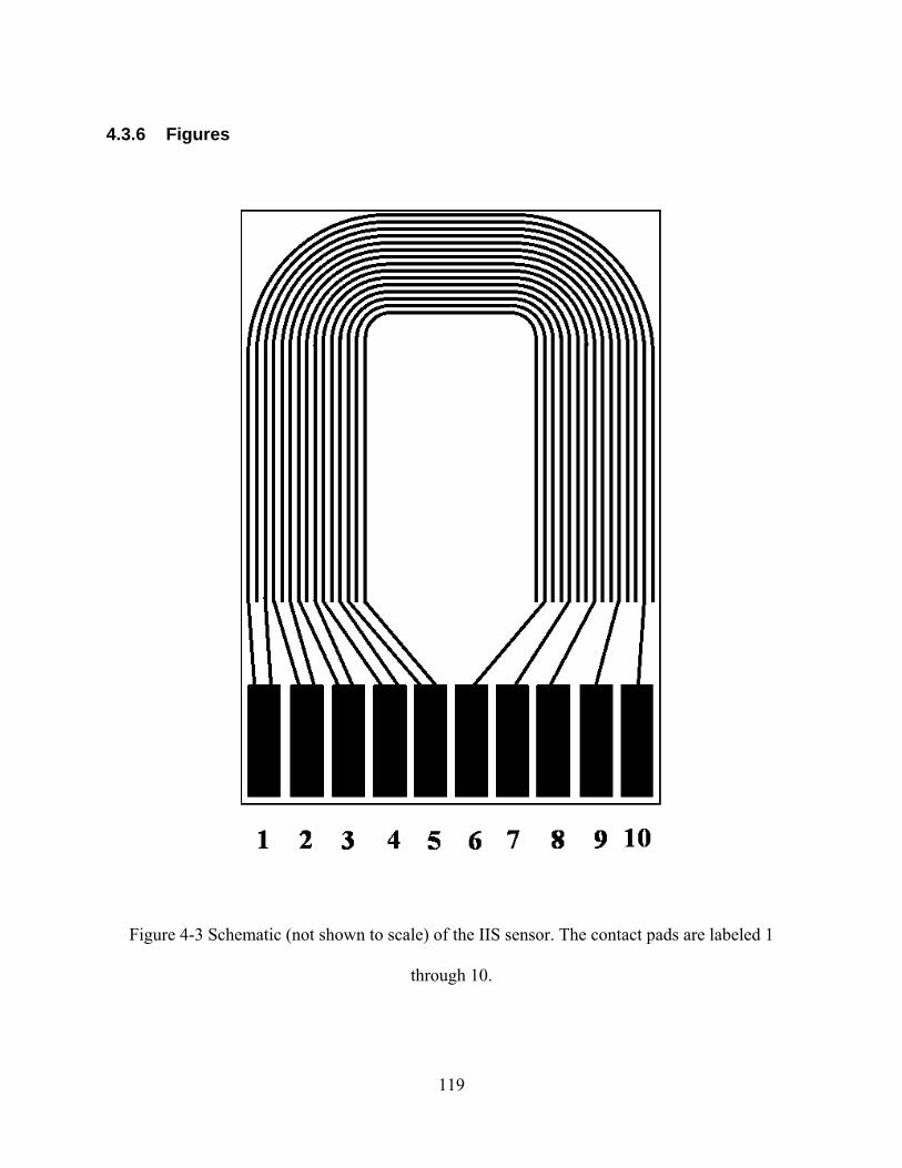
119

4.3.6 Figures

Figure 4-3 Schematic (not shown to scale) of the IIS sensor. The contact pads are labeled 1

through 10.

120

Figure 4-4 Photograph of the IIS sensor.

121

Figure 4-5 Schematic of the experimental set-up of the sensor and environmental chamber. The

path of diffusion is shown with the arrows.

122

51 µm thick Al foil backing31 µm thick PSA

diffusionfrom edge

sensor substrate

1 110

gold tracesfrom pads 1 & 10

(closest to free edge)

free edgeof sensor

Figure 4-6 Schematic of the side-view of the bonded PSA tape illustrating the path of diffusion

of acetone.

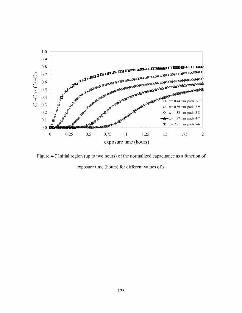
123

0.0

0.1

0.2

0.3

0.4

0.5

0.6

0.7

0.8

0.9

1.0

0 0.25 0.5 0.75 1 1.25 1.5 1.75 2

exposure time (hours)

C -C

0 / C

f -C

0

x = 0.44 mm, pads 1-10x = 0.89 mm, pads 2-9x = 1.33 mm, pads 3-8x = 1.77 mm, pads 4-7x = 2.21 mm, pads 5-6

Figure 4-7 Initial region (up to two hours) of the normalized capacitance as a function of

exposure time (hours) for different values of x.

124

0.0

0.2

0.4

0.6

0.8

1.0

0 0.5 1 1.5 2 2.5

distance from edge x (mm)

C -C

0 / C

f -C

0

56 hours12 hours6 hours4 hours2 hours1 hour45 min30 min10 min5 min t = 0

Figure 4-8 The concentration profile obtained from IIS sensor.

125

4.4 Diffusion of Water and Subsequent Debonding of a PSA Tape

4.4.1 Abstract

The effects of water absorption in a pressure sensitive adhesive tape were obtained using

interfacial impedance spectroscopy and a novel senor design described in other sections. The

results show characteristic behavior expected for adhesive debonding of coatings as a function of

environmental exposure time.

4.4.2 Materials and Experimental

The pressure sensitive adhesive tape used in this study is the “Quill Invisible Mending Tape”.

The PSA tape was exposed to water at room temperature. According to the manufacturer, the

pressure sensitive adhesive is acrylic based.

The novel IIS sensors used in this study can measure the impedance or capacitance of

mapped areas of the sensor defined with respect to the free edge of the coated sensor. Details of

the technique and experimental set-up can be found in Section 4.3 and in ref 125. The test

frequency was 1000 kHz. The substrate was the homogeneous low surface energy substrate. The

sensor was manufactured by taking the existing SiOx/Au/Ta energy substrate and depositing a

250 nm layer of silicon nitride and then a 135 nm layer of silicon carbide. To prepare the surface

of the substrate, they were first rinsed with HPLC grade isopropyl alcohol and then blown dry

with ultra-high purity nitrogen gas.

4.4.3 Results

The capacitance as a function of time is shown in Figure 4-9. After an initial region characteristic

of fluid diffusion into an adhesive coating, there is a significant increase in the capacitance at

126

approximately 15 hours. The dramatic increase in capacitance is attributable to a significant

increase in the concentration of fluid at the sensor interface resulting from the PSA tape

debonding. These results are similar to the expected results for an adhesive coating exhibiting

debonding (Figure 4-1). However, the characteristic lag time necessary for the fluid to migrate

across the surface to the respective pair of pads was not observed. This unexpected behavior is

either an artifact of the experimental set-up or, if these results truly reflect diffusion at the

interface, suggests that the fluid migrated instantly across the surface. Similar results were also

obtained for the diffusion of acetone into the aluminum foil PSA tape bonded to the SiN/SiC

surfaces. Nevertheless, these results illustrate that the sensor is capable of measuring adhesive

debonding. Adhesive failure is believed to occur from degradation of the interface and also due

to stress relaxation in the PSA tape backing. Stress relaxation caused the backing to shrink and

curl at the edges resulting in the tape lifting off the substrate.

4.4.4 Conclusion

The results of exposure of a PSA tape to water prove that the sensor is capable of measuring

adhesive debonding. Furthermore, the observed behavior follows similar trends that have been

observed by other researchers using single-frequency impedance spectroscopy.

127

4.4.5 Figures

1.50E-10

1.60E-10

1.70E-10

1.80E-10

1.90E-10

2.00E-10

2.10E-10

0 4 8 12 16 20 24

time (hours)

capa

cita

nce

(far

ads)

2.10E-10

2.20E-10

2.30E-10

2.40E-10

2.50E-10

2.60E-10

2.70E-10

capa

cita

nce

(far

ads)

x = 0.44 mmx = 0.89 mmx = 1.33 mmx = 1.77 mmx = 2.21 mm

debonding, t

Figure 4-9. Capacitance as a function of exposure time for the Quill pressure sensitive adhesive

tape in water.

128

4.5 Interfacial Diffusion of Aggressive Fluids into Epoxy Adhesive

Joints and Coatings Measured by Constant Frequency

Impedance Spectroscopy

4.5.1 Abstract

The diffusion of 0.1 M solution of NaOH into the commercial L4 epoxy adhesive joints and

coatings at 60°C was measured by constant frequency interfacial impedance spectroscopy and a

novel impedance sensor design described elsewhere. Several test specimens were investigated: 1)

the L4 adhesive sandwiched between two sensor substrates, 2) the L4 adhesive sandwiched

between two sensor substrates which have been coated with release agent, 3) the L4 adhesive

sandwiched between two sensor substrates that have been fabricated with a shim, and 4) the L4

adhesive coated on the sensor substrate approximately 50 microns thick (no sandwich). This

work suggest that the L4 adhesive interface is relatively durable and that differences in the

diffusivity between the bulk, non-bonded adhesive and the bonded adhesive can not be

distinguished using the current experimental set-up.

4.5.2 Research Objectives

The objective of this set of experiments was to address some fundamental questions regarding

the degradation of glassy adhesive joints by environmental stress (exposure to temperature and

fluid). Is fluid diffusion at the interface of an adhesive joint faster than fluid diffusion occurring

in the bulk adhesive? Which fluid chemistries promote interfacial diffusion and/or bulk

diffusion? Is the bulk diffusion coefficient a good indicator of the fluid’s aggressiveness and

mobility at an interface or adhesive joint? To attempt to answer these questions, the technique of

129

constant frequency interfacial impedance spectroscopy and a novel impedance sensor design

were used to try to measure the diffusion of 0.1 M NaOH into bonded epoxy adhesive

specimens. These novel IIS sensors measure the impedance of mapped areas of the sensor

defined with respect to the free edge of the coating. Consequently, these sensors can be used to

measure the distribution and transport of fluids at the interface. The adhesive was bonded

between two impermeable substrates (the sensors) to form a sandwich specimen geometry. In

such a geometry, because the backing is impermeable, fluid can enter the adhesive joint only

from the edges. From the edges, the fluid can diffuse in either the bulk adhesive material, along

the interface, or both. To determine the relative contribution to diffusion from the bulk and

interface, the relative rate of diffusion of fluid at the interface of the adhesive joints measured by

IIS could be compared to diffusion in bulk non-bonded adhesives. The study of the diffusion of

0.1 M NaOH is a worst case scenario. This fluid is water based, aggressive towards the interface,

and has a stronger impedance signal than pure water.

4.5.3 Experimental

4.5.3.1 Materials

The adhesive that was used in these experiments was a commercial filled epoxy known as the L4

adhesive. Details about the adhesive can be found in Section 3.4.3.1. The adhesive coating was

exposed to 0.1 M NaOH solution. The exposure temperature was 60° C. The high surface energy

sensor, which is mostly SiO and Au, was used as the substrate. Details of the sensor can be found

in Section 4.3 and also in the work of O’Brien et al.131

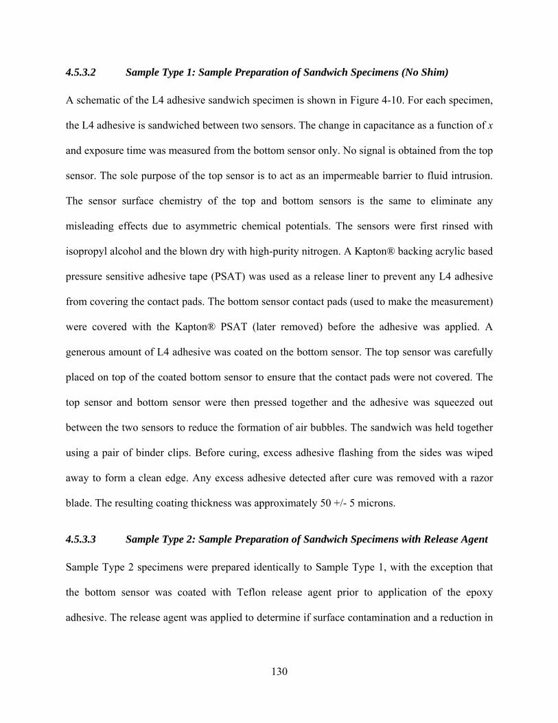
130

4.5.3.2 Sample Type 1: Sample Preparation of Sandwich Specimens (No Shim)

A schematic of the L4 adhesive sandwich specimen is shown in Figure 4-10. For each specimen,

the L4 adhesive is sandwiched between two sensors. The change in capacitance as a function of x

and exposure time was measured from the bottom sensor only. No signal is obtained from the top

sensor. The sole purpose of the top sensor is to act as an impermeable barrier to fluid intrusion.

The sensor surface chemistry of the top and bottom sensors is the same to eliminate any

misleading effects due to asymmetric chemical potentials. The sensors were first rinsed with

isopropyl alcohol and the blown dry with high-purity nitrogen. A Kapton® backing acrylic based

pressure sensitive adhesive tape (PSAT) was used as a release liner to prevent any L4 adhesive

from covering the contact pads. The bottom sensor contact pads (used to make the measurement)

were covered with the Kapton® PSAT (later removed) before the adhesive was applied. A

generous amount of L4 adhesive was coated on the bottom sensor. The top sensor was carefully

placed on top of the coated bottom sensor to ensure that the contact pads were not covered. The

top sensor and bottom sensor were then pressed together and the adhesive was squeezed out

between the two sensors to reduce the formation of air bubbles. The sandwich was held together

using a pair of binder clips. Before curing, excess adhesive flashing from the sides was wiped

away to form a clean edge. Any excess adhesive detected after cure was removed with a razor

blade. The resulting coating thickness was approximately 50 +/- 5 microns.

4.5.3.3 Sample Type 2: Sample Preparation of Sandwich Specimens with Release Agent

Sample Type 2 specimens were prepared identically to Sample Type 1, with the exception that

the bottom sensor was coated with Teflon release agent prior to application of the epoxy

adhesive. The release agent was applied to determine if surface contamination and a reduction in

131

the fracture resistance of the interface had any effect on the interfacial diffusion behavior in the

sandwich specimens.

4.5.3.4 Sample Type 3: Sample Preparation of Sandwich Specimens with Shim

Specimens fabricated with a glass shim in the center were also tested. A schematic of the side

view of a sandwich specimen with the glass shim is shown in Figure 4-11. A glass shim was

added to the center of the sandwich specimen to reduce the path of diffusion by half, from 5 mm

to 2.5 mm. The shim is approximately 4.75 mm wide, 20 mm long and 0.15 mm thick. The glass

shim occupies volume that would normally be filled with adhesive and any absorbed fluid. Note

that in the center of the sensor, from x = 2.5 - 5.0 mm, there are no conductive gold traces. The

glass shim is fastened to the bottom substrate in the correct center position by a small amount of

L4 adhesive which was pre-cured at 60°C for 30 minutes. The sample was then prepared

identically to Specimen Type 1.

4.5.3.5 Sample Type 4: Preparation of Adhesive Coatings

L4 adhesive applied to the sensor using a pneumatically driven doctor blade fabricated by

Hewlett-Packard. The resulting coating thickness was approximately 50 microns. The surface

was prepared identically to Specimen Type 1.

4.5.3.6 Constant Frequency Interfacial Impedance Spectroscopy

Details of the technique and experimental set-up can be found in Section 4.3 and also in the

International Journal of Adhesion and Adhesives131. The test frequency was 400 kHz. The

number of tested specimens for each condition was two and the exposure time was 30 days.

132

4.5.3.7 Concentration Profile

The normalized concentration (C*) of fluid as a function of exposure time in the adhesive joint

can be modeled using any of the several equations arising from Fick’s second law. For the

bonded L4 epoxy system, solutions to Fick’s Law do not account for the residual stress in the

joint, the change in stress state due to moisture absorption in the adhesive, or the non-Fickian

diffusion. For a semi-infinite planar interface, where x ≥ 0 at the interface, the concentration as a

function of distance from the specimen edge, x, and time, t, is expressed in Equation 4-10:52

Equation 4-10 ⎟⎟⎠

⎞⎜⎜⎝

⎛−=

−−

Dtxerf

CCCtxC

f 21

),(

0

0

where erf is the error function, D is the diffusion coefficient, C(x, t) is the concentration as a

function of distance from the edge, x , and exposure time, t, C0 is uniform initial concentration,

and Cf is the equilibrium concentration. Equation 4-10 may be applied to the measured

capacitance as a function of x and t because the concentration of fluid and capacitance are

expected to be proportional to one another. In this case the normalized concentration can be

replaced by the normalized capacitance.

Alternatively, the concentration profile in a polymer or adhesive joint of thickness, 2L, or

a coating of thickness L can be modeled using a solution to Fick’s law shown in Equation 4-11.45


⎜⎝⎛ +

⎥⎦

⎤⎢⎣

⎡ +−

+−

−=−− ∑

∞

= Lxn

LtnD

nCCCtxC

n

n

f 2)12(cos

4)12(exp

12)1(41

),(0

2

22

0

0 πππ

From either Equation 4-10 or Equation 4-11 the concentration profile as function of

exposure time and x can be calculated. The calculated concentration profile obtained from Fick’s

law can be compared to the concentration profile obtained from the capacitance data. To

determine the concentration profile from the capacitance date, the time to saturation and initial

133

and final capacitance values must be measured. By comparing the two concentration profiles, the

diffusivity, D, can be estimated.


4.5.4.1 Sample Type 1: Sandwich Specimens (No Shim)

The measured capacitance as a function of x and exposure time for samples 1 and 2 are shown in

Figure 4-12 and Figure 4-13 respectively. Recall that a value of x = 0 corresponds to the free

edge of the sensor. Qualitatively, the capacitance signal from the graphs show that the

capacitance increases with exposure time as expected. The change in the capacitance and the rate

of change of capacitance appear greater for smaller values of x. In addition, identical peaks and

valleys in the capacitance appear for all values of x. Theses peaks and valleys are suspected to be

noise and are not due to a change in concentration of fluid. To effectively model the diffusion

into the sandwich specimen, the change in capacitance and time to saturation must be known.

Unfortunately, these parameters are nearly impossible to quantify because of the substantial

noise in the data. As a result, no qualitative diffusion measurements were made. However, some

qualitative conclusions were made from these experiments.

The data obtained after 30 days of exposure suggests that the fluid concentration at the

surface is relatively low - lower than in any of the pressure sensitive adhesives tested (Section

4.3 and 4.6), and lower than L4 adhesive coatings damaged by hygroscopic cycling (Section

4.7). Under these test parameters, the concentration was low enough that the surface was not

significantly damaged to cause debonding (and the subsequent large change in capacitance).

Furthermore, the concentration is low enough that the change in capacitance due to fluid

absorption at the surface is not enough to overwhelm the signal-to-noise ratio.

134

The signal-to-noise ratio of the experiment is poor because the change in the capacitance

due to fluid absorption is small, on the order of 1 pF. This value was obtained from experiments

of thin L4 coatings where saturation was reached after only several hours (see Section 4.7). At

short experimental times, the effects of the poor signal-to-noise ratio are reduced because there is

less time for the baseline to change. The path of diffusion in the sandwich specimens is long (5

mm) and the time to 99% saturation of the adhesive in the sandwich specimen is approximately

440 days. Therefore, the 1 pF change in capacitance is spread out over a long period of time. As

shown in Figure 4-12 and Figure 4-13 the capacitance signal is susceptible to small but

misleading changes in the signal and baseline.

The expected concentration profile for diffusion of 0.1 M NaOH in the L4 adhesive at

60°C for the sandwich specimen (no shim, L = 5 mm) was calculated using Equation 4-11 based

on the diffusivity, D, of distilled water. The resulting concentration profile is shown in Figure

4-14. The concentration measured at x = 0.44, 0.89, 1.33, 1.77, and 2.21 are marked with dashed

vertical lines. The time for 80% of saturation (in concentration) at the outermost pair of pads

(pads 1-10, x = 0.44 mm) is approximately 25 days. After reaching 80% concentration,

additional increases in concentration were slow. Therefore, after 30 days of exposure, the signal

from the pad pair 1-10 is expected to reach roughly the maximum capacitance value. An

exposure time of 30 days therefore represents the expected minimum time necessary to obtain

the maximum capacitance change at x = 0.44 mm.

The signal-to-noise ratio can be improved by either increasing the mass of fluid absorbed

in the bulk and the surface or by decreasing the time-to-saturation. For most polymers, the

equilibrium mass of fluid absorbed can be increased by raising the exposure temperature.

However, the operating temperature of the instrument is already at a maximum. To decrease the

135

time-to-saturation, either the temperature can be increased or the path of diffusion can be

reduced. The path of diffusion was reduced by occupying a significant volume of the sandwich

specimen with a shim. Results from sandwich specimens that incorporate a shim are discussed in

a later section. Alternatively, the concentration of fluid at the surface could be increased by

reducing the toughness of the interface and making the adhesive susceptible to debonding.

4.5.4.2 Sample Type 2: Sandwich Specimens with Release Agent

The measured capacitance as a function of x and exposure time for samples 1 and 2 are shown in

Figure 4-15 and Figure 4-16 respectively. The results are similar to the samples without release

agent (Sample Type 1). The change in capacitance and time-to-saturation as a function of x can

not be quantified. In fact, the results from the release agent treated samples are more difficult to

quantify than the non-treated samples. The result from sample 1, shown in Figure 4-15, suggests

that despite degradation of the interface by the release agent, the epoxy still appears to remain

bonded to the surface. However, the result from sample 2, shown in Figure 4-16, shows that after

24 days the capacitance increases dramatically, suggesting that the adhesive has debonded up to

0.44 mm from the edge of the sensor.

4.5.4.3 Sample Type 3: Sandwich Specimens with Shim

The time to 99.9% saturation has been reduced from approximately 7 months to approximately 2

months by incorporating a spacer or shim in the sandwich specimen. The estimated concentration

profile for this specimen is shown in Figure 4-17. Examination of Figure 4-17 reveals that after

30 days of exposure the relative concentration is 80% or greater for x = 0.44 and 0.89 mm. In

contrast, in the Sample Type 3 specimens, after 30 days the relative concentration is 80% or

136

greater only for x = 0.44. Therefore, by using the spacer, the time to saturation has been reduced

and the instrument sensitivity has been increased.

The results from these experiments are shown in Figure 4-18 and Figure 4-19, where the

measured capacitance as a function of x and exposure time for sample 1 and 2, respectively, have

been graphed. Similar to the Sample Type 1 and 2, the results are difficult to quantify, despite the

significant reduction in the diffusion path length.

4.5.4.4 Sample Type 4: Adhesive Coating

Graphs of capacitance as a function of exposure time for the L4 coatings for samples 1 and 2 are

shown in Figure 4-20 and Figure 4-21, respectively. Examination of Figure 4-20 and Figure 4-21

reveals a dramatic change in capacitance after several days of exposure. This dramatic change in

capacitance is due to adhesive debonding an accumulation of fluid at the sensor surface. For the

adhesive coating, saturation was reached after only 1.4 hours. This experiment suggests that after

only several days of exposure to 0.1 M NaOH, the interface is significantly degraded in order to

result in coating delamination.

4.5.4.5 Discussion of Durability of Sandwich Specimens

In light of the results from the exposed adhesive coating (Section 4.5.4.4), the durability of the

sandwich specimens may be discussed. The durability of the L4 sandwich specimens is likely

attributable to the stress state of the adhesive sandwiched between the two impermeable

substrates. Abdel Wahab and coworkers studied the change in stress due to moisture diffusion in

epoxy adhesives bonded between aluminum.154 Using finite element analysis they report the

stress state in the adhesive at different exposure times. Of interest is their result after 6 weeks of

exposure where the normalized concentration in the adhesive they studied is similar to our

137

system after 30 days of exposure. Abdel Wahab and coworkers report that the peak peel stress is

reduced at the edge due to swelling and a reduction in modulus. In addition, changes in the

direction of shear stress and a reduction in the peak plastic strain were predicted. As a result,

they expected no reduction in joint strength, which agreed with their experimental adhesion

measurements of single lap joints. In contrast, the tested coatings exhibited debonding once the

crack driving energy due to residual stress exceeded the interfacial toughness. This published

work provides an additional example that coatings are typically less durable than adhesives

sandwiched between two substrates. These experimental results suggests that an interesting

future experiment would be to measure the diffusion of an aggressive fluid into an adhesive layer

sandwiched between the sensor and a flexible, yet impermeable backing, with good chemical

resistance (e.g tantalum film).

4.5.5 Conclusions

Constant frequency interfacial impedance spectroscopy was utilized to investigate the diffusion

of 0.1 M NaOH into bonded L4 epoxy adhesive sandwich joints and coatings. A number of

conclusions have been made that are unique to this adhesive system, but have wider implications.

For the sandwich specimens, the sensitivity of the instrument and sensors was not sufficient to

determine the change in capacitance or time to saturation, two important diffusion parameters,

within a reasonable error. The sandwich adhesive bond appears durable and, within the

sensitivity of the instrument, does not appear to have any fluid accumulation or debonding. In

contrast, the adhesive coating exhibited delamination after only several days of exposure. This

work provides an additional example that coatings are typically less durable than adhesives

sandwiched between two substrates. These results suggest that the experimental set-up must be

modified in order to obtain enough sensitivity to detect the migration of fluids into durable

138

structural adhesive joints. Recommendations for improving the resolution of the instrument are

discussed in Section 0.

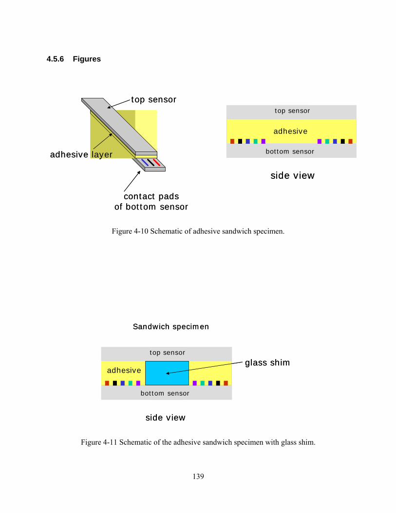
139

4.5.6 Figures

adhesive

bottom sensor

top sensor

contact padsof bottom sensor

adhesive layer

top sensor

side view

adhesive

bottom sensor

top sensor

contact padsof bottom sensor

adhesive layer

top sensor

side view

Figure 4-10 Schematic of adhesive sandwich specimen.

Sandwich specimen

adhesive

bottom sensor

top sensor

side view

glass shim

Sandwich specimen

adhesive

bottom sensor

top sensor

side view

glass shim

Figure 4-11 Schematic of the adhesive sandwich specimen with glass shim.

140

1.470E-10

1.475E-10

1.480E-10

1.485E-10

1.490E-10

0 5 10 15 20 25 30 35

exposure time (days)

capa

cita

nce

(fara

ds)

1.365E-10

1.370E-10

1.375E-10

1.380E-10

1.385E-10

x = 0.89 mm, pads 2:9x = 1.33 mm, pads 3:8x = 1.77 mm, pads 4:7x = 0.44 mm, pads 1:10

Figure 4-12 The capacitance as a function of exposure time (days) for the L4 adhesive sandwich

specimens Type 1 Sample 1 exposed to 0.1 M NaOH.

1.45E-10

1.46E-10

1.47E-10

1.48E-10

1.49E-10

1.50E-10

1.51E-10

1.52E-10

0 5 10 15 20 25 30 35


capa

cita

nce

(far

ads)

1.703E-10

1.708E-10

1.713E-10

1.718E-10

1.723E-10

1.728E-10

x = 0.44 mm, pads 1:10x = 0.89 mm, pads 2:9x = 1.33 mm, pads 3:8x = 1.77 mm, pads 4:7x = 2.21 mm, pads 5:6

1.45E-10

1.46E-10

1.47E-10

1.48E-10

1.49E-10

1.50E-10

1.51E-10

1.52E-10

0 5 10 15 20 25 30 35


capa

cita

nce

(far

ads)

1.703E-10

1.708E-10

1.713E-10

1.718E-10

1.723E-10

1.728E-10



specimens Type 1 Sample 2 exposed to 0.1 M NaOH.

141

0.0

0.2

0.4

0.6

0.8

1.0

0.50.60.70.80.91

x / L

C*

1 day11 days22 days31 days44 days

0.0

0.2

0.4

0.6

0.8

1.0

0.50.60.70.80.91

x / L

C*

1 day11 days22 days31 days44 days

Figure 4-14 Normalized concentration (C*) as a function of normalized distance from the edge (x

/ L). x / L = 1 is the edge and x / L = 0 is the center of the sensor. This is for the sample without a

shim, where L = 5.0 mm. The vertical dashed lines represent the value of x that each pair of pads

measures for pads 1-10 (x / L = 0.91), 2-9, 3-8, 4-7, and 5-6 (x / L = .56).

142

1.38E-10

1.39E-10

1.40E-10

1.41E-10

1.42E-10

0 5 10 15 20 25 30 35

time (days)

capa

cita

nce

(Far

ads)

1.57E-10

1.58E-10

1.59E-10

1.60E-10

1.61E-10



specimens Type 2 Sample 1 exposed to 0.1 M NaOH. The surface was treated with release agent.

1.41E-10

1.42E-10

1.43E-10

1.44E-10

1.45E-10

1.46E-10

1.47E-10

0 5 10 15 20 25 30 35


capa

cita

nce

(fara

ds)

1.60E-10

1.61E-10

1.62E-10

1.63E-10

1.64E-10

1.65E-10

1.66E-10



specimens Type 2 Sample 2 exposed to 0.1 M NaOH. The surface was treated with release agent.

143

0

0.2

0.4

0.6

0.8

1

00.20.40.60.81

x / L

C*

7 hours3 days6 days8 days11 days17 days27 days55 days

0

0.2

0.4

0.6

0.8

1

00.20.40.60.81

x / L

C*

7 hours3 days6 days8 days11 days17 days27 days55 days

Figure 4-17 Normalized concentration (C*) as a function of normalized distance from the edge (x

/ L). x / L = 1 is the edge and x / L = 0 is the center of the sensor. This is for the sample with a

shim, where L = 2.5 mm. The vertical dashed lines represent the value of x that each pair of pads

measures for pads 1-10 (x / L = 0.91), 2-9, 3-8, 4-7, and 5-6 (x / L = .56).

144

1.460E-10

1.465E-10

1.470E-10

1.475E-10

1.480E-10

1.485E-10

1.490E-10

0 5 10 15 20 25 30 35


capa

cita

nce

(far

ads)



specimens Type 3 Sample 1 exposed to 0.1 M NaOH. The sample was equipped with a shim.

1.465E-10

1.470E-10

1.475E-10

1.480E-10

1.485E-10

1.490E-10

0 5 10 15 20 25 30 35


capa

cita

nce

(far

ads)



specimens Type 3 Sample 2 exposed to 0.1 M NaOH. The sample was equipped with a shim.

145

-2.0E-10

-1.0E-10

0.0E+00

1.0E-10

2.0E-10

3.0E-10

4.0E-10

0 1 2 3 4 5 6


capa

cita

nce

(fara

ds)


Figure 4-20 The capacitance as a function of exposure time (days) for the L4 adhesive coatings

Type 4 Sample 1 exposed to 0.1 M NaOH.

1.3E-10

1.8E-10

2.3E-10

2.8E-10

3.3E-10

0 1 2 3 4 5 6 7


capa

cita

nce

(fara

ds)


Figure 4-21 The capacitance as a function of exposure time (days) for the L4 adhesive coatings

Type 4 Sample 2 exposed to 0.1 M NaOH.

146

4.6 Moisture Diffusion from the Edge in Bonded UV Curable Pressure

Sensitive Adhesives Measured by Constant Frequency

Impedance Spectroscopy

4.6.1 Abstract

Moisture diffusion into a series of UV curable pressure sensitive adhesives was measured using

constant frequency interfacial impedance spectroscopy and a novel impedance sensor design.

Adhesives Research Incorporated of Glen Rock, Pennsylvania supplied and fabricated the

samples. Either a permeable poly(ethylene terephthalate) backing or an impermeable glass

backing was used to control the path of diffusion into the bonded adhesive. Several different

types of adhesives were tested. Samples were conditioned in either 60° water or in 60°C 100%

relative humidity environments. This work illustrates the wide variety of diffusion behaviors of

bonded adhesives and demonstrates the utility of the IIS technique as an effective tool for

screening adhesive formulations.

4.6.2 Experimental

4.6.2.1 General Adhesive Description and Sample Preparation

The adhesives used in this study were manufactured by Adhesives Research Incorporated. The

details of the structure are proprietary. However, the adhesives are UV curable and are epoxy

based. Acrylate groups provide the necessary groups to make the adhesive UV curable. The

uncured adhesive is tacky and will fibrillate readily when stretched.

Samples were prepared at Adhesive Research Incorporated. The high surface energy

sensor substrates (SiO/Au) were utilized in this research. The sensor surfaces were prepared by

147

first rinsing with isopropyl alcohol and then blow-drying the sensor with high-purity nitrogen.

The PSA adhesive film initially has two transfer liner layers on either side of the film to facilitate

handling. A single liner was removed and the adhesive was carefully applied to the sensor so that

no bubbles are formed. The second transfer layer was removed and either the glass or

poly(ethylene terephthalate) (PET) backing was applied. The adhesives were 63.5 microns (2.5

mils) thick and the PET liner was 50.8 microns (2.0 mils thick).The glass backing was carefully

applied to ensure no air bubbles were formed. The specimen was then placed in an oven at 65 °C

for 1-2 minutes to soften the adhesive and promote wetting. Some specimens were not subjected

to the 65 °C oven step. The specimen is then hand pressed and exposed to UV dose to cure. Note

some samples were uncured. Bonded specimens were then immediately stored in dessicant.

4.6.2.2 Experimental

The adhesive formulation is denoted as ARiA (ARi id# 480-52-A). ARiA was tested under

several conditions where the effects of the backing properties, the state of water, sample

preparation (and consequently the interfacial toughness) and cure were investigated. The samples

are desiganted:

1. ARiA (no 65 °C step) PET backing in 60 °C liquid water

2. ARiA (no 65 °C step) PET backing in 60 °C water vapor

3. ARiA (no 65 °C step) Glass backing in 60 °C liquid water

4. ARiA (no 65 °C step) Glass backing in 60 °C water vapor

5. ARiA (with 65 °C step) no cure, Glass backing in 60 °C water vapor

6. ARiA (with 65 °C step) cured, Glass backing in 60 °C water vapor

148

For these samples, “no 65” denotes that the during the sample fabrication process, specimens

were not exposed to the 65°C oven for 1-2 minutes. Exposure of the sample to the 65 °C step

improved adhesion.

To control the path of diffusion into the bonded adhesive, either a permeable PET

backing (Figure 4-22) or an impermeable glass backing were utilized (Figure 4-23). As shown in

Figure 4-22, the PET backing allows for moisture transport through the top of the PET backing

and adhesive in the direction of the interface and also from the edge of the sensor. Note that the

path of diffusion is much shorter, and therefore faster, through the top of the bonded adhesive

than from the edge of the sensor. The impermeable glass backing controls the path of diffusion

so that fluid enters the adhesive from the edge of the sensor only and results in the highest

concentration of fluid at the sensor edge. Unfortunately, the bulk diffusion behavior of the

adhesive could not be accurately measured. Therefore, the moisture diffusion behavior

determined from IIS could not be correlated to bulk diffusion in the adhesive.


4.6.3.1 ARiA (no 65 °C) PET Backing in 60 °C Liquid Water

A graph of the capacitance as a function of x and exposure time is shown in Figure 4-24 for

ARiA (no 65 °C) PET backing in 60°C liquid water. The capacitance changes for each value of x

are essentially the same value. This suggests that the diffusion of water to the electrode interface

is predominantly though the top of the backing and that diffusion from the edge is not

significant. Additional evidence suggesting diffusion from the edge is not significant comes from

the graph of the capacitance as a function of x and exposure time for the first few hours, shown

in Figure 4-25. The necessary lag time for the water to diffuse through the film to the surface and

149

begin to accumulate is apparent in Figure 4-25. This lag time is independent on the distance from

the edge of the sensor, x. Also of interest is the change in capacitance is positive up to

approximately 3.5 hours and negative following that time. The dramatic change in slope after

approximately 3.5 days does not necessarily mean the adhesive has been saturated. The change

in slope is likely due to a change in the phase angle brought about by a large fluid concentration.

4.6.3.2 ARiA (no 65 °C) PET Backing in 60 °C Water Vapor

The graph of the capacitance as a function of x and exposure time is shown in Figure 4-26 for

ARiA (no 65 °C) PET backing in 60 °C water vapor. For this adhesive (ARiA no 65 °C PET

backing), the shape of the capacitance curve was essentially the same as for the 60°C liquid

water and water vapor condition. The time when the capacitance dramatically changes slope was

approximately 4.5 days. In addition, the magnitude of the change in capacitance observed for

samples exposed to 60°C relative humidity was much less than in the 60°C water. The difference

in the change in capacitance is probably not due to a different concentrations of water at the

sensor surface because the time to saturation were similar and because there was no theoretical

difference between the water transport mechanism for liquid water and water vapor.155

Additional samples are needed to determine the reproducibility and error of these experiments.

Note that it would be advantageous to use water vapor when studying the absorption of water

into adhesives, since this would eliminate any misleading effects caused by liquid water

evaporation.

4.6.3.3 ARiA (no 65 °C) Glass Backing in 60°C Liquid Water

The graph of the capacitance as a function of x and exposure time is shown in Figure 4-27 for

ARiA (no 65 °C) Glass backing in 60 °C liquid water. As expected, the change in capacitance

150

was greater closer to the edge of the sensor and there was also a lag time necessary for the fluid

to diffuse from the edge and across the sensor surface. These trends are more easily observed in

the graph of the resistance as a function of x and exposure time is shown in Figure 4-28. After

roughly 20 to 25 days the adhesive was saturated up to a value of x = 1.77 mm.

4.6.3.4 ARiA (no 65 °C) Glass Backing in 60 °C Water Vapor

A graph of the capacitance as a function of x and exposure time is shown in Figure 4-29 for

ARiA (no 65 °C) Glass backing in 60 °C water vapor. Also a plot of the resistance as a function

of x and exposure time is shown in Figure 4-30. Again, the expected trends in capacitance and

resistance were observed. After roughly 20 to 25 days the adhesive was saturated up to a value of

x = 1.77 mm. The large change in capacitance, visible lag time and saturation time from the

ARiA (no 65 °C) adhesive with a glass backing (liquid and vapor water) indicate that moisture

diffuses into the ARiA at larger concentrations relative to the epoxy adhesives studied in Section

4.5. As discussed previously, moisture diffusion into the bonded PSA could occur from the either

the interface, the bulk, or from both sources.

4.6.3.5 ARiA (With 65 °C) no Cure Glass Backing in 60 °C Water Vapor

The uncured (no UV exposure) ARiA adhesive formulation with a glass backing was exposed to

60°C water vapor. Here, the sample underwent the 65 °C step for 1-2 minutes. The sample was

exposed for approximately 10 days. Two samples were tested to demonstrate the repeatability of

the experiment. The measured capacitance as a function of x and exposure time for samples 1

and 2 are shown in Figure 4-33 and Figure 4-32, respectively. In sample 1, the uncured adhesive

exhibited a peak in the capacitance after only 6 hours for all values of x. In sample 2, the uncured

adhesive exhibited a peak in the capacitance after only 8 hours for all values of x. In both

151

samples, a small lag time (up to 2 hours) necessary for the moisture to migrate from the edge of

the specimen was observed. The similar behavior between sample 1 and 2 illustrates the

repeatability of the experiments. No significant difference in the lag time or peak in capacitance

was observed for different values of x. This suggests that the fluid rapidly migrates across the

sensor surface and that moisture transport from the interface must be significant. If diffusion

occurred predominantly in the bulk and from the edge of the specimen, then a lag time would

have been observed. The data suggest that the uncured adhesive is not durable and that moisture

diffused into the adhesive rapidly (less than several days). Comparing the cured and uncured

systems strongly suggest that curing the adhesive is essential to increasing the durability.

4.6.3.6 ARiA (With 65°C) Cured with Glass Backing in 60 °C Water Vapor

The measured capacitance as a function of x and exposure time is shown in Figure 4-33 and

Figure 4-34, respectively. The UV cured samples exhibited a minimal change in capacitance of

approximately 1 – 2 pico-farads. Both samples exhibited a greater change in capacitance and a

peak in the capacitance values of x = 0.44 and 0.89 mm. This result and others indicate that these

experiments have good repeatability. Furthermore, these results suggest that the change in

capacitance at these values of x is likely to have a physical meaning and is not just a result of

noise in the data. We can speculate that the increase in capacitance at the edge of the specimen is

due to greater swelling and a greater concentration of moisture at the edge than in the center of

the specimen. A large jump in the capacitance is observed in sample 1 and 2 after 8 days of

exposure; however, it is unclear if the increase is due to noise or a real physical event in this

case. This relatively small change in capacitance at the center of the specimen is similar in

magnitude to the tested L4 epoxy adhesives exposed to the aggressive fluid (Section 4.5). The

similar behavior with the L4 epoxy adhesives suggests the UV cured PSA may be as effective as

152

the epoxy. Comparing the results from the ARiA adhesive with and without the 65 °C step,

indicates that significant more durability is imparted on the sample when the 65 °C step was

employed, presumable due to better wetting and a corresponding increase in the interfacial

toughness. Both conditions (with and without the 65 °C step) utilize the same adhesive and

therefore have similar bulk (non-bonded) adhesive diffusion rates. Differences in the diffusion

behavior detected by IIS are therefore a result of differences in the interface. These experiments

show that the sensor can distinguish differences in the interface durability. The two extremes of

moisture absorption behavior have been measured. In the case of poor durability (AriA UV no

cure and AriA cured no 65 °C step), changes in capacitance indicate a significant contribution to

diffusion from the interface. In the case of good durability (L4 adhesive and AriA cured with the

65 °C step), changes in capacitance due to fluid absorption are small and the capacitance signal

is subject to noise.

4.6.4 Conclusions

A wide variety of diffusion behavior has been illustrated by studying several different types of

UV curable pressures sensitive adhesives. Utilizing constant frequency IIS, differences were

observed among samples with different paths of diffusion into the bonded adhesive, state of cure,

and interfacial toughness. Most importantly is the dramatic difference in diffusion behavior

between relatively non-durable adhesives and durable adhesives. For non-durable adhesives,

changes in capacitance indicate a significant contribution to diffusion from the interface. For

durable adhesives, changes in capacitance due to fluid absorption are relatively small and the

capacitance signal is subject to noise.

153

4.6.5 Figures

Diffusionfrom edge

sensor substrate

UV PSA

PET Backing

Diffusion through PET film

Figure 4-22 Schematic of the profile view of the adhesive with the PET backing bonded to the

sensor. The paths of diffusion are illustrated with the red arrows.

Diffusionfrom edge

sensor substrate

UV PSA

Glass Backing

Glass is impermeable

Figure 4-23 Schematic of the profile view of the adhesive with the glass backing bonded to the

sensor. The path of diffusion is illustrated with the red arrows.

154

0E+00

1E-10

2E-10

3E-10

4E-10

5E-10

6E-10

7E-10

8E-10

0 5 10 15 20 25 30 35


capa

cita

nce

(fara

ds)


-

Figure 4-24 The measured capcitance (pF) as function of exposure time (days) for the AriA

adhesive with the PET backing in 60°C water.

0E+00

1E-10

2E-10

3E-10

4E-10

5E-10

6E-10

7E-10

8E-10

0 1 2 3 4 5


capa

cita

nce

(fara

ds)


-

Figure 4-25 The measured capcitance (pF) as function of exposure time (days) for the AriA

adhesive with the PET backing in 60°C water. The first few hours are shown to illustrate the lag

time necessary for the fluid to diffuse to the sensor surface.

155

1.2E-10

1.4E-10

1.6E-10

1.8E-10

2.0E-10

2.2E-10

0 5 10 15 20 25 30 35


capa

cita

nce

(fara

ds)


Figure 4-26 The measured capacitance (pF) as function of exposure time (days) for the AriA

adhesive with the PET backing in 60°C 100% relative humidity.

1.3E-10

1.4E-10

1.5E-10

1.6E-10

1.7E-10

1.8E-10

1.9E-10

0 5 10 15 20 25 30 35


capa

cita

nce

(fara

ds)



adhesive with the glass backing in 60°C water.

156

0.0E+00

2.0E+04

4.0E+04

6.0E+04

8.0E+04

1.0E+05

1.2E+05

0 5 10 15 20 25 30 35


resis

tanc

e (o

hms)


Figure 4-28 The measured resistance (ohms) as function of exposure time (days) for the AriA

adhesive with the glass backing in 60°C water.

1.4E-10

1.6E-10

1.8E-10

2.0E-10

2.2E-10

0 5 10 15 20 25 30 35


capa

cita

nce

(fara

ds)



adhesive with the glass backing in 60°C 100% relative humidity.

157

0E+00

2E+04

4E+04

6E+04

8E+04

1E+05

0 5 10 15 20 25 30 35


resis

tanc

e (o

hms)


Figure 4-30 The measured resistance (ohms) as function of exposure time (days) for the AriA

adhesive with the glass backing in 60°C 100% relative humidity.

1.45E-10

1.50E-10

1.55E-10

1.60E-10

1.65E-10

1.70E-10

1.75E-10

0 2 4 6 8 10 12


capa

cita

nce

(Far

ads)


Figure 4-31 The measured capacitance (pF) as function of exposure time (days) for the ARi 480-

52-A No UV cure (Sample 1)

158

1.49E-10

1.51E-10

1.53E-10

1.55E-10

1.57E-10

1.59E-10

0 2 4 6 8 10


capa

cita

nce

(fara

ds) x = 0.44 mm, pads 1:10

x = 0.89 mm, pads 2:9x = 1.33 mm, pads 3:8x = 1.77 mm, pads 4:7


52-A No UV cure (Sample 2)

1.39E-10

1.40E-10

1.41E-10

1.42E-10

1.43E-10

1.44E-10

1.45E-10

1.46E-10

1.47E-10

0 2 4 6 8 10 12


capa

cita

nce

(fara

ds)

1.940E-10

1.945E-10

1.950E-10

1.955E-10

1.960E-10

1.965E-10

1.970E-10

1.975E-10

1.980E-10x = 0.44 mm, pads 1:10x = 1.33 mm, pads 3:8x = 1.77 mm, pads 4:7x = 0.66 mm, pads 1-2


52-A High UV cure (Sample 1).

159

1.46E-10

1.48E-10

1.50E-10

1.52E-10

1.54E-10

1.56E-10

0 2 4 6 8 10 12 14 16


capa

cita

nce

(fara

ds)



52-A High UV cure (Sample 2).

160

4.7 Durability of Adhesive Coatings Subjected to Hygroscopic

Cycling Measured by Constant Frequency Impedance

Spectroscopy

4.7.1 Abstract

The technique of constant frequency interfacial impedance spectroscopy (IIS) coupled with a

novel interdigitated electrode sensor design were used to investigate the effects of hygroscopic

cycling on the durability of epoxy adhesive coatings. Using IIS enabled measurement of the

change in capacitance resulting from fluid absorption as a function of the distance from the edge

of the sensor, x, and the number of exposure cycles. This information was utilized to determine

the number of cycles required to initiate adhesive failure and also the “apparent crack length”

growth rates of the failure as a function of the number of exposure cycles. During a single cycle

the coated specimens were first exposed to fluid at 60°C for 24 hours, then cooled to room

temperature in the fluid environment for 30 minutes, and then dried in a dessicator (~ 5 %

relative humidity) for an additional 24 hours. It is in the last stage of the cycle, during the drying

step, that the adhesive coatings debonded. Evidence for adhesive debonding was evident from

large changes in the capacitance resulting from interfacial displacement of the adhesive and the

large concentration of fluid at the substrate sensor surface. The number of cycles until failure

was determined as a function of coating thickness, fluid environment, and sensor surface

chemistry.

161

4.7.2 Introduction

4.7.2.1 Residual Stresses in Adhesive Joints

Internal residual stresses can significantly affect the durability of adhesives and composites 8-11.

These stresses can cause adhesive failure by leading to the formation of cracks 11 which tend to

initiate at bimaterial interface corners or edges.156,157 Residual stress in adhesives joints and

coatings can originate from processing or solidification of the adhesive. Heating or cooling

where there is a difference in the coefficient of thermal expansion (CTE) between the adhesive

and substrate lead to such stresses, as do the absorption of moisture and other fluids.11,158,159

Internal residual stresses in adhesive coatings can either be contractive or expansive in nature.160

Contractive internal stresses impart a tensile stress on the coating and develop from volume

shrinkage typical of coating formation and/or thermal contractive stresses. Volume shrinkage

during coating formation can result from either cure shrinkage or from solvent loss, or a

combination of the two. Contractive stresses in adhesives arise from the CTE mismatch between

the substrate and adhesive coating described above. The usual case is where the CTE of the

substrate (O ~ 1-10 for glasses) is less than the CTE of the polymer (O ~ 60 - 100). Under such

conditions, if the stresses are (equal) biaxial, the residual stress σr in the coating (or sandwich

specimen) can be estimated from the following expression:126,161,162

Equation 4-12 TEr ∆∆

−−= α

νσ

)1(

where E is the modulus of the coating, ∆α = αa - αs is the difference between the linear

coefficient of thermal expansion of the adhesive coating αa and substrate αs, ∆T = T – TSFT is the

difference between the temperature of the adhesive T and the stress free temperature TSFT, and v

is the Poisson ratio of the adhesive coating (typically ca. 0.4 for an epoxy). The stress free

162

temperature is near the glass transition of the adhesive; however, the stress free temperature can

vary by as much as 40°C because of differences in cooling the adhesive (quench vs. slow

cool).163 Based on a stress singularity approach, Lefebvre and co-workers predicted that with

high glass transition materials, where (Tcure - TSFT ) ~ 200, under unfavorable conditions (high

modulus, high CTE, poor adhesion) residual stresses can initiate debonding at interface corners,

where cracks tend to initiate.156,157

Crack initiation at the edge of an adhesive bond is exacerbated at interface corners where

the coating shear stresses due to CTE mismatch are at a maximum. These shear stresses decrease

away from the edge and are zero in the center of the coating.162 The tensile residual stresses, on

the other hand is zero at the edges and at a maximum in the center of the adhesive joint. In the

work of Humfield and Dillard12, crack initiation at the edge of adhesive joints was attributed to

shear and peeling stresses at the interface edge resulting from residual stresses. These residual

stresses were generated by adhesive shrinkage during cure and the discussed difference in CTE

between the adhesive and substrate. They suggested that crack growth will tend to occur at lower

temperatures when the residual stresses and strain energy release rate are highest.12

Although the residual stress is independent (as Equation 4-12 reveals) of the coating

thickness, the strain energy release rate G or crack driving energy is proportional to the film

thickness h and is expressed in Equation 4-13.126,162

Equation 4-13 E

hZG r )1(2 υσ −

=

where Z is equal to 1.028 during crack initiation and 0.5 for steady state crack growth.

Furthermore, a critical thickness hc is predicted above which debonding is predicted to occur 162:

Equation 4-14 )1(

12 υσ −

Γ=

r

cc

EZ

h

163

where Γc is the debonding energy or toughness of the interface.

Volume expansion of the coating by swelling with water and/or other fluids, or an

increase in temperature can cause the internal stresses to be compressive.160 Similar to residual

stresses cased by CTE mismatch, the residual stress due to swelling can be expressed as:

Equation 4-15 swellingrE εν

σ)1( −

−=

where εswelling is the strain induced by swelling or absorption of the penetrant. The value of εswelling

can be expressed in terms of a linear hygroscopic expansion coefficient that is a function of

temperature 161:

Equation 4-16 TEr ∆∆

−−= β

νσ

)1(

where ∆β = βa - βs is the difference between the linear hygroscopic expansion coefficient of the

adhesive coating, βa, and of the substrate, βs, and ∆T = T – T is the temperature difference.

Alternatively, the value of εswelling can be expressed in terms of a linear hygroscopic expansion

coefficient that is a function of absorbed mass:162

Equation 4-17 MEr ∆∆

−−= β

νσ

)1(

where ∆M is the change in absorbed mass. Vanlandingham et al. found that for epoxy resins

cured with amines that the value of β was 0.22 mm per mm per wt% and also found reductions in

Tg ranging from 5 – 20 °C.56

It should also be noted that stresses influence the absorption of moisture. Yaniv and Ishai

showed that for epoxies the maximum amount of absorbed moisture is not stress dependent;

164

however, in tension the diffusion rate increased and in compression the diffusion rate was

reduced.164

It is relevant to note Weitsman’s results for an adhesive constrained between two rigid

adherends, which apply to an adhesive undergoing expansion due to either elevated temperature

or moisture absorption.165 Weitsman showed that during the initial stage of the swelling process:

1) the resulting normal stresses are compressive at the edge of the joint, 2) there is a peak tensile

stress at a place slightly inside the interface, and 3) the stress is zero far away from the edge. For

the fully saturated (equilibrium) condition, the normal tensile stresses are at a maximum at the

edge of the joint. For thin films the stresses were found to be slightly compressive away from

edge, similar to the stress state in a peel test geometry. Furthermore, during the drying process

of an initially swollen adhesive similar peel stresses can be generated at the edge.

4.7.2.2 Thermal and Hygroscopic Cycling of Adhesive Joints and Coatings

Thermal cycling can also dramatically reduce the lifetime of an adhesive bond. Humfeld and

Dillard describe the mechanism for adhesive failure due to thermal cycling.12 They propose that

residual stresses are built up with each cycle until the available strain energy release rate is large

enough to initiate debonding. Residual stress build up is caused by three factors: structural

changes occurring at elevated temperature due to expansion of the adhesive, the accompanying

increase in molecular mobility, and the relaxation of the resulting compressive stresses. The

resulting structural changes in the adhesive are then frozen into the adhesive upon cooling. With

each cycle, hey found structural changes cause the adhesive to shrink, leading to a build up of

residual stresses.

Hygroscopic cycling or changing the content of absorbed moisture or other fluids can

produce the same effect as temperature cycling.12 This is because both increasing the temperature

165

and the fluid content of the adhesive are processes that cause an increase the volume of the

adhesive and also increase frequency and amplitude of molecular motions in the polymer chains.

Fluid desorption produces a similar effect as decreasing the temperature by reducing the

adhesive volume and slowing down molecular motions. The effects of cycling and subsequent

adhesive failure may be more dramatic if the temperature and fluid content are reduced

simultaneously. Fluid absorption can also make the adhesive more susceptible to the deleterious

effects of residual stress by changing the chemistry of the interface, by reducing the toughness of

the interface, or by migration to the interface to form a weak boundary layer.

In addition to the changes in structure by temperature and hygroscopic cycling, physical

aging can also induce harmful structural changes in adhesives. Physical aging is the phenomenon

associated with conformational changes of the polymer chain backbone leading to a reduction in

free volume and a change in structure that occurs below the glass transition temperature.166

Physical aging can lead to adverse effects such as an increase in density and elastic modulus and

a reduction in the impact strength, fracture toughness, and rate of creep and stress relaxation.

4.7.3 Experimental

4.7.3.1 Constant Frequency Interfacial Impedance Spectroscopy

The novel IIS sensors used in this study can measure the impedance or capacitance of mapped

areas of the sensor defined with respect to the free edge of the coated sensor. Details of the

technique and experimental set-up can be found in Section 4.3 and also in the International

Journal of Adhesion and Adhesives.131 The test frequency was 400 kHz in the work described in

this section. Using the technique of constant frequency IIS and the novel sensor design we have

measured the change in capacitance as a function of the distance from the edge of the sensor, x,

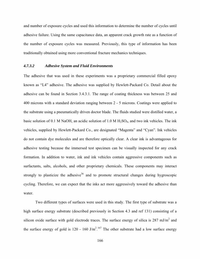
166

and number of exposure cycles and used this information to determine the number of cycles until

adhesive failure. Using the same capacitance data, an apparent crack growth rate as a function of

the number of exposure cycles was measured. Previously, this type of information has been

traditionally obtained using more conventional fracture mechanics techniques.

4.7.3.2 Adhesive System and Fluid Environments

The adhesive that was used in these experiments was a proprietary commercial filled epoxy

known as “L4” adhesive. The adhesive was supplied by Hewlett-Packard Co. Detail about the

adhesive can be found in Section 3.4.3.1. The range of coating thickness was between 25 and

400 microns with a standard deviation ranging between 2 - 5 microns. Coatings were applied to

the substrate using a pneumatically driven doctor blade. The fluids studied were distilled water, a

basic solution of 0.1 M NaOH, an acidic solution of 1.0 M H2SO4, and two ink vehicles. The ink

vehicles, supplied by Hewlett-Packard Co., are designated “Magenta” and “Cyan”. Ink vehicles

do not contain dye molecules and are therefore optically clear. A clear ink is advantageous for

adhesive testing because the immersed test specimen can be visually inspected for any crack

formation. In addition to water, ink and ink vehicles contain aggressive components such as

surfactants, salts, alcohols, and other proprietary chemicals. These components may interact

strongly to plasticize the adhesive36 and to promote structural changes during hygroscopic

cycling. Therefore, we can expect that the inks act more aggressively toward the adhesive than

water.

Two different types of surfaces were used in this study. The first type of substrate was a

high surface energy substrate (described previously in Section 4.3 and ref 131) consisting of a

silicon oxide surface with gold electrode traces. The surface energy of silica is 287 mJ/m2 and

the surface energy of gold is 120 - 160 J/m2.167 The other substrate had a low surface energy

167

consisting mostly of silicon carbide and some silicon nitride. The surface free energy of silicon

carbide is 35 – 60 J/m2 168. The sensor was manufactured by taking the existing high surface

energy substrate and depositing a 250 nm layer of silicon nitride followed by a 135 nm layer of

silicon carbide. A schematic of the high and low surface energy substrate sensors are shown in

Figure 4-35. To prepare the surface of the substrate, they were first rinsed with HPLC grade

isopropyl alcohol and then blown dry with ultra-high purity nitrogen gas. The L4 adhesive was

applied immediately thereafter, cured at 140°C for 30 minutes and cooled slowly (approximately

30 minutes) to room temperature. Coated sensors were stored in a dessicator (5% relative

humidity) prior to testing.

4.7.3.3 Description of Environmental Cycles

The cycle used in this study can be divided into three stages:

Stage 1. 15 minute preheat in 60°C air followed by immersion in 60°C fluid environment for 24

hours.

Stage 2. Cooling from 60°C to room temperature in fluid environment (approximately 30

minutes).

Stage 3. Drying of the adhesive coating at 5% relative humidity for 24 hours.

In the initial stage the dry epoxy coated sensor is placed in the convection oven to equilibrate at

60°C for approximately 15 minutes. The adhesive coating is then immersed in the fluid

environment at 60°C. During this initial stage, the capacitance is recorded as a function of

exposure time. Exposure to the fluid environment is approximately 24 hours. It should be

emphasized that the change in capacitance is measured only during the fluid exposure step (stage

168

1). In the second stage, the adhesive (still immersed in the fluid environment) is removed from

the oven and allowed to cool off to room temperature (approximately 20°C). This step takes

approximately 30 minutes, and eliminates any thermal shock to the adhesive coating which

would accelerate the failure process. As pointed out by Humfield and Dillard, faster changes in

temperature increase the rate of stress development and the magnitude of stress, and therefore

reduce adhesive bond life.12 In the third stage, the adhesive coating is dried in a dessicator (~ 5%

relative humidity) for 24 hours. In this last stage, significant debonding is believed to take place.

4.7.3.4 Common Features of the Adhesive Debonding Measurements: Failure Criteria

and Apparent Crack Length

4.7.3.4.1 Capacitance Changes Due to Fluid Absorption in an Undamaged Coating

Using the technique of constant frequency IIS and the novel impedance sensor design, data was

obtained on the change in capacitance as a function of the distance from the edge of the sensor, x,

and the number of exposure cycles. The absorbed volume of fluid at the sensor surface is

proportional to the measured change in capacitance. In undamaged coatings the change in

capacitance due to fluid absorption is roughly 1 pF (pico-Farad) for both the low and high

surface energy sensors. The change in capacitance is the difference between the capacitance

measured after 24 hours of fluid exposure and the initial dry capacitance (t = 0 hours). Figure

4-36 illustrates the change in capacitance as a function of exposure time typically observed

during the initial cycle.

4.7.3.4.2 Capacitance Changes Due to Fluid Absorption in an Damaged Coating

In the event of adhesive debonding, a dramatic increase in capacitance is detected due to

displacement of the adhesive from the substrate surface and an accumulation of fluid at the

169

sensor surface. For the epoxy adhesive and fluids studied, debonding occurs during the final

stage of the cycle in the dessicator. Evidence for adhesive debonding during this drying process

is obtained from the change in capacitance measured in the subsequent cycle as the coated sensor

is immersed in the fluid environment. As an example, Figure 4-37 illustrates the dramatic change

in capacitance for adhesive coatings that have debonded in the drying stage of the previous cycle.

Figure 4-37 shows that the capacitance continues to rise dramatically for up to several

hours. This observation suggests that either further crack growth occurs in the fluid exposure

step, or that this is simply a result of additional fluid diffusion. Nonetheless, the most significant

damage is believed to have has occurred in the previous cycle.

For each cycle, the change in capacitance due to fluid absorption and/or debonding as a

function of x can be determined from graphs similar to Figure 4-36 and Figure 4-37. The data

from each cycle can then be plotted collectively as shown in Figure 4-38. The change in

capacitance as a function of x and number of cycles for the Magenta ink vehicle is displayed in

Figure 4-38. For clarity, the capacitance is plotted on a log scale Figure 4-38.

4.7.3.4.3 Values of the Change in Capacitance

The change in capacitance observed in a damaged coating is depends on several factors such as

the concentration of fluid at the surface, the total area of debonding, the fluid chemistry, surface

of the sensor (SiO2/Au vs. SiC/SiN) and the specific pair of connection pads (or value of x) from

which the measurement was made. These many factors, and others not discussed, significantly

affect the capacitance measurements and make it difficult to obtain qualitative information about

the actual concentration of fluid at the sensor surface. The change in capacitance due to the

presence of fluid at a debonded region of the sensor surface can be as large as 1000 pF for the

low surface energy (SiC/SiN) sensor. For the high surface energy (SiO/Au) sensor, with the

170

exception of a distilled water environment, the change in capacitance due to adhesive debonding

is positive at low concentrations while at high concentration the change in capacitance is

negative. Therefore adhesive coatings bonded to the high surface energy sensor exhibited a

negative capacitance if complete coating debonding has occurred. This effect is due to the highly

ionic nature of the non-water fluids which can cause a large change in the detected phase angle

of the complex impedance.

4.7.3.4.4 The Minimum Change in Capacitance Suggesting Adhesive Failure; Apparent Crack

Length

Using the novel impedance sensor design, the capacitance can be measured as a function of

location from the edge of the bond, x. Because the change in capacitance is roughly proportional

to the change in concentration of fluid at the surface, damaged regions of the adhesive also can

be detected as a function of x. As expected, crack initiation always started at the free edge of the

coated sensor (x = 0 mm) and crack growth was always in the direction toward the center of the

sensor. If such a crack has advanced in the coated sensor from the edge, then it is expected that

the change in capacitance will be large in the debonded regions and low in the bonded regions.

For several reasons explained below, a change in capacitance exceeding a value of 10 pF is

indicative of adhesive failure. Conversely, a change of less than 10 pF suggests that the adhesive

coating is undamaged. Therefore, if the crack has advanced 1.33 mm, then for values of x less

than or equal to 1.33 we expect a change in capacitance greater than 10 pF. For the inner section

of the senor where x > 1.33 mm, we would observe a change in capacitance less than 10 pF.

171

4.7.3.4.5 Justification for the Failure Criteria

As suggested previously, a measured change in capacitance of 10 pF or greater is believed to

indicate that significant debonding has occurred at that particular value of x. Also mentioned

previously, the change in capacitance due to fluid absorption in an undamaged coating is roughly

1 pF. A value of 1 pF agrees well with rough estimates based on the rules of mixtures (Section

4.2.2) for an epoxy adhesive absorbing 1 - 2 wt% of fluid in the bulk. Based on the same

calculation, a change of 10 pF corresponds to an epoxy adhesive absorbing 15 wt% of fluid.

Assuming a typical number such that the adhesive absorbs roughly 2.5 wt% in fluid at

equilibrium in the bulk, any amount exceeding this indicates a surplus of fluid most likely due to

debonding and displacement of the adhesive by the fluid. Therefore, 10 pF and an absorption of

15 wt% of fluid is a conservative estimate of the change in capacitance indicating damage to the

coating.

Utilizing a value greater than 10 pF also ensures that the change in capacitance is due to

the presence of the fluid and not to other outside or uncontrollable sources of capacitance

changes. The most prevalent source of noise is the unavoidable change in capacitance due to

changing the contact pressure and position of the sensor within the fixture. The change due to

this effect is roughly 2 – 4 pF.

Changes in capacitance less than 10 pF also appear to be reversible in some cases.

Several examples were found where the capacitance changed by as much as 8 pF during a cycle,

whereas on the subsequent cycle exhibited a change in capacitance of only 1 – 2 pF. In addition,

samples that have exhibited a change in capacitance greater than 10 pF were visually inspected -

it was confirmed that these adhesive coatings had areas of debonding.

172

4.7.3.4.6 Defining an Apparent Crack

The measured crack length is “apparent” because the capacitance measurements are a global

average of the damage to the sensor. Crack formation may not be entirely symmetric around the

edge of the sensor and debonding may have occurred at capacitance changes less than (or greater

than) 10 pF. In many cases the crack growth was observed visually to be non-uniform. In

addition, the change in capacitance can vary due to variation in the concentration of fluid at the

surface and the total area of debonding, as well as differences in fluid chemistry and the specific

pair of pads from which the measurement was taken. Hence an apparent crack is detected while

its location has some uncertainty.

4.7.3.4.7 Cycles Until Failure

Assessment of the degree of damage to the adhesive incurred from the drying process is made

during the subsequent cycle. Therefore when referring to the number of cycles until failure, the

specific reference is to the number of cycles until failure is observed or detected by the change in

capacitance.


4.7.4.1 Effect of Water

The graph of the number of cycles until failure as a function of coating thickness for both the low

and high surface energy sensors is shown in Figure 4-39. For the purpose of discussion,

specimens have been categorized based on the thickness of the coating: 1) less than 50 microns,

2) between 50 – 150 microns and 3) greater than 150 microns. The number of samples tested is

listed in Table 4-2. The number of cycles until failure in Figure 4-37 has been categorized

173

according to the coating thickness and shown in Table 4-3. Coatings adhered to both substrate

chemical types and less than 50 microns and did not exhibit any crack initiation or growth for as

many as 20 cycles. For samples with a thickness in the range of 50 – 150 microns, the number of

cycles until failure was 11.3 +/- 2.1, identical for both substrate surface chemistries. For samples

with a thickness greater than 150 microns, the number of cycles until failure was 4.0 +/- 1.0 and

4.7 +/- 1.5 for the high and low surface energy substrates, respectively. These results support the

idea that decreasing the thickness of the coating improves adhesive durability by reducing the

crack driving energy attributable to residual stresses.

Table 4-2 The number of samples tested as a function of coating thickness and sensor surface

chemistry. The fluid environment is water.

Coating Thickness

(microns) SiO/Au Surface SiC/SiN Surface

< 50 2 2

50 - 150 3 3

> 150 3 3

174

Table 4-3 The number of cycles until failure as a function of coating thickness and substrate

surface chemistry. The fluid environment is water. The average and a single standard deviation

are listed.

Coating Thickness


< 50 Greater than 20 Greater than 20

50 - 150 11.3 +/- 2.1 11.3 +/- 2.1

> 150 4.0 +/- 1.0 4.7 +/- 1.5

The numbers of cycles until failure of both the low and high surface energy sensors were

similar. This is not surprising, given that adhesion for both surfaces can be attributed to forces

resulting from secondary bonds (hydrogen-bonds, van der Waal’s, etc.). Therefore, both

substrates may be subject to similar adhesive failure mechanisms. For samples less than 50

microns, the build up of residual stresses was not enough to increase the available strain energy

to cause debonding despite the degradation of the interface that may have occurred. This

behavior is in sharp contrast to samples with a coating thickness greater than 50 microns which

failed catastrophically. To be clear, catastrophic failure is defined by the initiation and formation

of a crack 2.2 mm in length, the maximum detectable value of x (obtained from the innermost

pair of contact pads). Failure is presumably attributable to residual stress build up increasing the

available strain energy such that it exceeds the interfacial toughness. The catastrophic adhesive

failure is also different than what is observed for other environmental fluids where crack initiated

occurred at the sensor edge and crack growth occurred over a period of many cycles in the

direction of the center of the sample.

175

For water at 60°C, the respective time to saturation as a function of coating thickness is

shown in Table 4-4. The time to saturation (99.9%) was calculated from Equation 4-18130,169 and

a diffusion coefficient of 1.3 x 10-8 cm2/s.36

Equation 4-18 D

Ltsat

2467.0 ⋅=

Where L is the coating thickness and D is the diffusion coefficient. The results listed in Table 4-4

show that the 50 micron coatings are saturated within a few hours. Coatings approximately 250

microns in thickness are not saturated on the first cycle. Saturation may or may not occur on a

subsequent cycle(s) if the fluid begins to accumulate in the adhesive. The time to saturation for

the other fluids has not been measured. However, similar diffusion coefficients are expected

because the major component of each fluid is water.

Table 4-4 The time to saturation as a function of coating thickness for the L4 adhesive at 60°C

water.

Coating Thickness

(microns)

Time To Saturation

(hours)

50 1.5

100 5.5

150 12

200 22

250 34

300 49

176

4.7.4.2 Effect of 0.1 M Sulfuric Acid

The number of cycles until failure as a function of coating thickness and sensor surface

chemistry for the 60°C 0.1 M sulfuric acid environment is shown in Figure 4-40. The number of

samples tested is listed in Table 4-5. The average number of cycles until failure as function of

coating thickness and surface chemistry are listed in Table 4-6. As expected, the acidic

environment is more aggressive than the distilled water environment. Again, no difference in the

number of cycles until failure between the low and high surface energy sensors was observable.

The dependence of the durability on coating thickness was also less pronounced than for the

specimens exposed to water.

In contrast to samples exposed to the water environment, adhesive failure for the acidic

samples was not catastrophic. For samples with a range of coating thickness less than 50

microns, the graphs of the apparent crack length as a function of the number of exposure cycles

are shown in Figure 4-41 and Figure 4-42, for the low and high energy surfaces, respectively. In

each case, 2 cycles are required to initiate crack growth that begins from the free edge of the

sensor. Once the crack growth has been initiated, the crack grows at a rate of 1.1 mm/cycle and

0.8 +/- 0.4 mm/cycle for the low and high surface energy sensors, respectively.

177

Table 4-5 The number of samples tested as a function of coating thickness and sensor surface

chemistry. The fluid environment is 0.1 M sulfuric acid.

Coating Thickness


< 50 2 2

50 - 150 2 3

> 150 2 2


surface chemistry for the 0.1 M sulfuric acid environment. The average and a single standard

deviation are shown.

Coating Thickness


< 50 5.0 +/- 1.4 4.0 +/- 0.0

50 - 150 2.5 +/- 0.7 2.3 +/- 0.6

> 150 2.5 +/- 0.7 2.0 +/- 0.0

4.7.4.3 Effect of 1.0 M NaOH

The number of cycles until failure as a function of coating thickness and surface chemistry for

the 60°C 1.0 M NaOH environment is shown in Figure 4-43. The number of samples tested for

each coating thickness range and surface was two. These results show that for the entire range of

178

coating thicknesses, the adhesive coating fails catastrophically after only 2 cycles. This is clearly

the most aggressive of the five tested fluids. No difference between the low and high surface

energy sensors was observable. The aggressiveness of the fluid may be attributable to hydrolysis

of the epoxy-substrate bond near the interface, or to an actual etching of the substrate.

All adhesive coatings, independent of the thickness, failed catastrophically after the

drying stage of the first cycle. In contrast to the other fluid environments, reducing the thickness

below 50 microns does not reduce the energy available for crack growth to extend the life of the

adhesive coating in the NaOH environment. The adhesive coatings greater than 250 microns

which are predicted to not saturate (see Table 4-4) also fail catastrophically after the drying stage

of the first cycle. This suggests that the adhesive does not need to be saturated for the interface to

be degraded substantially. This is consistent with the idea that concentration in the adhesive only

needs to exceed a critical concentration to degrade the interface. An additional mechanism for

adhesive failure that would not require the adhesive to be saturated could be due to degradation

of the adhesive at the edge of the specimen. At the edge of the specimen, the diffusion path is

short and the concentration of fluid is high. At the edge, the bulk adhesive and interface can be

degraded enough to cause crack initiation. Once the crack is initiated, the adhesive can fail

catastrophically if the residual stress and the coating thickness are large enough. An alternative

and less substantiated is that the fluid diffuses rapidly at the interface into the adhesive joint and

degrades the adhesive joint much faster than expected.

4.7.4.4 Effect of Cyan Ink Vehicle


the 60°C Cyan ink vehicle environment is shown in Figure 4-44. The number of samples tested

is shown in Table 4-7. The average number of cycles until failure as function of coating

179

thickness and surface chemistry are listed in Table 4-8. For adhesive coatings greater than 50

microns, catastrophic failure occurs after only 2 cycles. No difference between the low and high

surface energy sensors was observable. These results show that by reducing the coating thickness

below 50 microns, the lifetime of the adhesive joint may be extended beyond two cycles.

Furthermore, these results also suggest that Cyan is more aggressive than either water or acid,

but not as aggressive as the basic solution. For the Cyan ink vehicle, adhesive failure was not

catastrophic. The graphs of the apparent crack length as a function of the number of exposure

cycles are shown in Figure 4-45 and Figure 4-46 for both the low and high energy surface

substrates respectively. The crack growth rate determined from IIS is 0.9 +/- 0.3 mm/cycle and

1.0 +/- 0.2 mm/cycle for the low and high surface energy substrates, respectively.

Table 4-7 The number of samples tested for the range of coating thickness for each surface

chemistry.

Coating Thickness


< 50 4 4

50 - 150 4 3

> 150 2 2

180


surface chemistry for the Cyan ink vehicle environment. The average and a single standard


Coating Thickness


< 50 3.5 +/- 0.6 3.5 +/- 0.6

50 - 150 2.0 +/- 0.0 2.0 +/- 0.0

> 150 2.0 +/- 0.7 2.0 +/- 0.0

4.7.4.5 Effect of Magenta Ink Vehicle


the 60°C Magenta ink vehicle environment is shown in Figure 4-47. The number of samples

tested as function of coating thickness and surface chemistry is shown in Table 4-9. The average

number of cycles until failure as function of coating thickness and surface chemistry are listed in

Table 4-10. Coatings of 50 microns or less tend to be more durable than coatings with a greater

thickness. Thin coatings (< 50 microns) bonded to the low energy SiC/SiN surface had a greater

durability than the high energy SiO/Au surface. The Magenta ink vehicle is the only fluid where

differences between the two surface chemistries were observed; however, these differences are

observed only for coatings less than 50 micron. The low surface energy sensor appears more

durable than the high surface energy sensor. This phenomenon may be fundamentally similar to

the increase in adhesion energy for two low energy surfaces (like the epoxy and substrate) in the

presence of high surface energy fluid like water. The graphs of the apparent crack length as a

181

function of the number of exposure cycles are shown in Figure 4-48 and Figure 4-49 for the low

and high energy surface chemistries, respectively. The rate of apparent crack growth determined

by IIS was 0.4 +/- 0.1 and 1.0 +/- 0.2 mm/cycle for the low and high surface energy surface

substrate respectively.

Table 4-9 The number of samples tested as a function of coating thickness and surface chemistry.

The fluid environment is Magenta ink vehicle.

Coating Thickness


< 50 3 3

50 - 150 3 2

> 150 2 3


surface chemistry for the Magenta ink vehicle environment. The average and a single standard


Coating Thickness


< 50 3.3 +/- 0.6 6.33 +/- 0.6

50 - 150 2.0 +/- 0.0 2.0 +/- 0.0

> 150 2.0 +/- 0.0 2.0 +/- 0.0

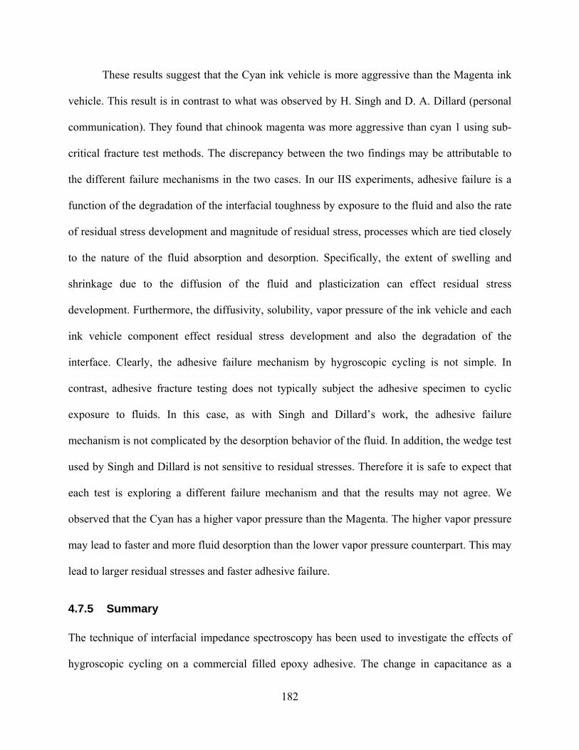
182

These results suggest that the Cyan ink vehicle is more aggressive than the Magenta ink

vehicle. This result is in contrast to what was observed by H. Singh and D. A. Dillard (personal

communication). They found that chinook magenta was more aggressive than cyan 1 using sub-

critical fracture test methods. The discrepancy between the two findings may be attributable to

the different failure mechanisms in the two cases. In our IIS experiments, adhesive failure is a

function of the degradation of the interfacial toughness by exposure to the fluid and also the rate

of residual stress development and magnitude of residual stress, processes which are tied closely

to the nature of the fluid absorption and desorption. Specifically, the extent of swelling and

shrinkage due to the diffusion of the fluid and plasticization can effect residual stress

development. Furthermore, the diffusivity, solubility, vapor pressure of the ink vehicle and each

ink vehicle component effect residual stress development and also the degradation of the

interface. Clearly, the adhesive failure mechanism by hygroscopic cycling is not simple. In

contrast, adhesive fracture testing does not typically subject the adhesive specimen to cyclic

exposure to fluids. In this case, as with Singh and Dillard’s work, the adhesive failure

mechanism is not complicated by the desorption behavior of the fluid. In addition, the wedge test

used by Singh and Dillard is not sensitive to residual stresses. Therefore it is safe to expect that

each test is exploring a different failure mechanism and that the results may not agree. We

observed that the Cyan has a higher vapor pressure than the Magenta. The higher vapor pressure

may lead to faster and more fluid desorption than the lower vapor pressure counterpart. This may

lead to larger residual stresses and faster adhesive failure.

4.7.5 Summary

The technique of interfacial impedance spectroscopy has been used to investigate the effects of

hygroscopic cycling on a commercial filled epoxy adhesive. The change in capacitance as a

183

function of x was measured to study adhesive durability as a function of coating thickness, fluid

environment, and surface chemistry.

Several observations are put forth as a result of the experiments.

1. The durability of the adhesive coatings is improved by reducing the adhesive coating

thickness, presumably due to a reduction in the available energy for crack growth from residual

stress.

2. Experimental evidence supports the general observation that adhesive cracks tend to initiate at

free edges. Furthermore, crack initiation occurred in the drying stage of cyclic environmental

swelling and drying.

3. Constant frequency impedance spectroscopy and a novel senor design were successfully used

to determine the number of cycles until failure and the rate of apparent crack length growth as a

function of the number of exposure cycles.

184

4.7.6 Figures

Silicon Wafer Substrate

1.2 µm Gold traces Silicon oxide0.06 µm Tantalum


0.135 µm SiC0.25 µm SiN

Deposit

*Not to scale


1.2 µm Gold traces Silicon oxide0.06 µm Tantalum


0.135 µm SiC0.25 µm SiN

Deposit

*Not to scale

Figure 4-35 Schematic (not to scale) of the high surface energy substrate (shown in top) and the

low surface energy substrate (shown in bottom)

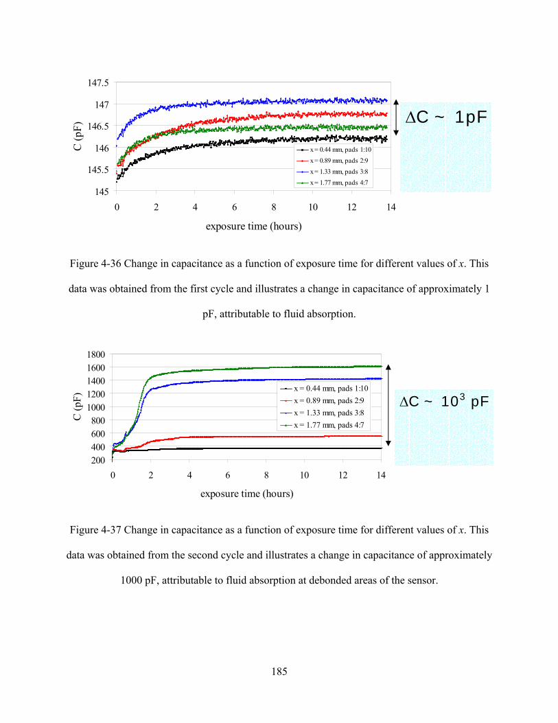
185

Figure 4-36 Change in capacitance as a function of exposure time for different values of x. This

data was obtained from the first cycle and illustrates a change in capacitance of approximately 1

pF, attributable to fluid absorption.

Figure 4-37 Change in capacitance as a function of exposure time for different values of x. This

data was obtained from the second cycle and illustrates a change in capacitance of approximately

1000 pF, attributable to fluid absorption at debonded areas of the sensor.

145

145.5

146

146.5

147

147.5

0 2 4 6 8 10 12 14


C (p

F)


∆C ~ 1pF

200400600800

10001200140016001800

0 2 4 6 8 10 12 14


C (p

F)


∆C ~ 103 pF

186

0.1

1

10

100

1000

0 0.5 1 1.5 2 2.5

x (mm)

Log

[del

ta C

]

cycle 1cycle 2cycle 3cycle 4cycle 5cycle 6cycle 7cycle 8cycle 9cycle 10

Figure 4-38 The change in capacitance due to fluid absorption plotted on a log scale as a

function of the distance from the edge of the sensor, x, for different exposure cycles. This

for a 30 micron coating exposed to the Magenta ink vehicle.

187

0

5

10

15

20

25

0 50 100 150 200 250 300

coating thickness (microns)

# of

cyc

les

SiO/Au surfaceSiC/SiN surface

Figure 4-39 The number of cycles until failure as a function of coating thickness for the 60°C

distilled water environment.

188

01234567

0 50 100 150 200 250


# of

cyc

les SiO/Au surface

SiC/SiN surface

Figure 4-40 The number of cycle until failure as a function of coating thickness for the 60°C 1 M

sulfuric acid environment.

189

00.5

11.5

22.5

3

0 1 2 3 4 5

Cycles

appa

rent

cra

ck le

ngth

(mm

) sample 1sample 2

Figure 4-41 The apparent crack length (mm) as a function of exposure cycles. This for coatings

less than 50 microns bonded to the silcon carbide surface and exposed to the sulfuric acid

solution.

190

0

0.5

11.5

2

2.5

0 1 2 3 4 5 6 7

Cycles

appa

rent

cra

ck le

ngth

(mm

) sample 1sample 2


less than 50 microns bonded to the silcon oxide and gold surface and exposed to the sulfuric acid

solution.

191

0

1

2

3

0 100 200 300 400


# of

cyc

les


Figure 4-43 The number of cycle until failure as a function of coating thickness for the 60°C 0.1

M NaOH environment.

192

0

1

2

3

4

5

0 100 200 300 400


# of

cyc

les


Figure 4-44 The number of cycle until failure as a function of coating thickness for the 60°C

Cyan ink vehicle environment.

00.5

11.5

22.5

3

0 1 2 3 4 5

Cycles

appa

rent

cra

ck le

ngth

(mm

) sample 1sample 2sample 3sample 4


less than 50 microns bonded to the silcon carbide surface and exposed to the Cyan ink vehicle.

193

00.5

11.5

22.5

3

0 1 2 3 4 5

Cycles

appa

rent

cra

ck le

ngth

(mm

)

sample 1sample 2sample 3


less than 50 microns bonded to the silcon oxide and gold surface and exposed to the Cyan ink

vehicle.

194

012345678

0 100 200 300 400


# of

cyc

les


Figure 4-47 The number of cycle until failure as a function of coating thickness for the 60°C

Magenta ink vehicle environment.

195

00.5

11.5

22.5

3

0 1 2 3 4 5 6 7 8

Cycles

appa

rent

cra

ck le

ngth

(mm

)

sample 1sample 2sample 3


less than 50 microns bonded to the silcon carbide surface and exposed to the Magenta ink

vehicle.

196

00.5

11.5

22.5

3

0 1 2 3 4 5

Cycles

appa

rent

cra

ck le

ngth

(mm

)sample 1sample 2sample 3


less than 50 microns bonded to the silcon oxide and gold surface and exposed to the Magenta ink

vehicle.

197

4.8 Recommendations and Modifications for Constant Frequency

Interfacial Impedance Spectroscopy

4.8.1 Abstract

Modifications are recommended to achieve the full potential of the novel sensor design for

interfacial impedance spectroscopy and in the experimental set-up for the study of diffusion in

adhesive joints. In addition, some experimental details are discussed for any future investigators.

4.8.2 Sources of Signal Noise

There are many sources of noise in the experiment. The most prevalent and serious is the

constant change in temperature of the experimental equipment outside the oven. To a lesser

extent, the activity of persons and other instruments in the room is also a source. The noise in the

capacitance signal was found to closely follow changes in the temperature. The activity of the

room also followed the temperature fluctuations and therefore can not be ruled out as a possible

source of error. Most importantly, opening and closing the oven door should be avoided. The

first recommendation would be to reduce temperature changes by containing the switch box,

impedance analyzer, and oven in a controlled temperature environment.

4.8.3 Recommended Modifications

The twisted cables of the connectors should be replaced with shielded coaxial cables. This

should significantly reduce any noise in the data as well as reduce the difference in the initial

capacitance among the different pairs of contact pads.

Several modifications to the sensor design are recommended to improve the sensitivity of

the instrument. The modifications are based on the work of Senturia and Garverick who designed

198

an interdigitated impedance sensor with built-in amplification that is sensitive at frequencies as

low as 1 Hz. In addition, they utilize a second or reference transistor so that the response of the

sensor to background effects that are not of interest can be cancelled out. In the literature, they

refer to the technique as “microdielectrometry”. A detailed description of the sensor which

includes the circuit diagrams can be found in ref 170, 171, and 172.170,171,172 This

microdielectrometry device was utilized to study the cure of two epoxy systems173 and as a

humidity sensor.174

The ability to test a large number of specimens without monopolizing the instrument for

one would be an ideal situation. This could be accomplished by conditioning the samples in a

separate environment and then periodically removing the samples for testing. A reproducible

signal would be a prerequisite. One obstacle to creating a reproducible signal is creating a virtual

identical low resistance, reproducible contact between the fixture and sensor contact pads. A new

contact device could be fabricated which would likely involve a clamp or pressure contact and

would move away from the spring set-up in the current fixtures.

The basic sensor geometry could be modified in several ways. To increase the

capacitance, the conductive traces could be made longer and the space between the traces could

be reduced. An example in the literature has the conductive traces as small as 8 microns wide

with an 8 micron spacing.174 In addition, the region in the center of the sensor where no traces

are present should be eliminated. This region effectively increases the diffusion path length by a

factor of two and substantially increases the time to saturation by a factor of four.

The available frequency range of the instrument is limited and spans only over 3 decades,

ranging from a minimum of 75 kHz to a maximum of 10 MHz. The choice of the test frequency

is based on two factors. As the frequency is decreased, the impedance signal becomes more

199

sensitive to water and the baseline quality is reduced. Equation 4-19 illustrates how the

frequency is related to the capacitance and resistance:

Equation 4-19 π2EfIC

∆∆

=

where ∆I is the complex sinusoidal current measurement, ∆E is the complex sinusoidal voltage

(usually the input signal),and f is the applied frequency. This relation suggests as the frequency

is decreased the instrument sensitivity (the ratio of the output signal to input signal) must

increase proportionally.142

A wide range of frequencies would provide quantitative information into the underlying

mechanism of diffusion and fluids at the interface of adhesive joints. Unlike the qualitative

information yielded by constant frequency testing, multi-frequency impedance spectroscopy can

be used to distinguish absorbed water and condensed water, as well as other phenomena. To

obtain this information, an equivalent circuit model is used to fit the impedance data as a

function of frequency data.139

200

5 CONCLUDING REMARKS

The durability of adhesive joints was characterized using the shaft-loaded blister test and a novel

impedance sensor design. The SLBT was demonstrated to be a simple and convenient method

for characterizing the environmental degradation of adhesive bonds. The traditional SLBT was

adapted to constant-load sub-critical fracture testing. The plateau velocity and threshold value of

G were shown to be not solely controlled by bulk diffusion of fluids into the adhesive. The

capability of the sensor was demonstrated by measuring the diffusion the diffusion of acetone

parallel to the bondline into a PSA tape.

Diffusion of moisture into durable adhesives can not be quantified due to the limited

sensitivity of the current experimental set-up. The technique of IIS was demonstrated to be

sensitive to the interfacial toughness of UV curable pressure sensitive adhesives. Moreover, this

sensor was shown to be an invaluable tool in quantifying the effects of hygroscopic cycling and

was used to measure the rate of apparent crack growth in adhesive coatings.

This research has provided additional evidence of the harmful effects of moisture,

temperature, hydroscopic cycling and has provided the adhesives industry two new and useful

test methods for adhesive evaluation.

201

6 REFERENCES:

(1) Kinloch, A. J. Adhesion and Adhesives: Science and Technology; Chapman and Hall: New York, 1987.

(2) Dickstein, P. A.; Spelt, J. K.; Sinclair, A. N.; Bushlin, Y. Materials Evaluation 1991, 1498-1515.

(3) Nguyen, T.; Byrd, E.; Bentz, D. Journal of Adhesion 1995, 48, 169-194. (4) Bowden, F. P.; Throssell, W. R. Nature 1957, 167, 601. (5) Kinloch, A. J. Journal of Adhesion 1979, 10, 193-219. (6) Weitsman, Y. J. Mechanics of Time Dependent Materials 2000, 4, 107-126. (7) Reboa, P. F., Personal Communication (8) Kook, S. Y.; Dauskardt, R. H. Journal of Applied Physics 2002, 91, 1293-1303. (9) Piens, M.; DeDeurwaerder, H. Progress in Organic Coatings 2001, 43, 18-24. (10) Clyne, T. W. Key Engineering Materials 1996, 116-117, 307-330. (11) Sato, K. Progress in Organic Coatings 1980, 8, 143-160. (12) Humfeld Jr, G. R.; Dillard, D. A. Journal of Adhesion 1998, 65, 277-306. (13) Sung, N. H. (14) McBreirty, V. J.; Keely, C. M.; Coyle, F. M.; H., X.; K., V. J. Faraday Discussions 1996,

103, 255-268. (15) Antoon, M. K.; Koenig, J. L. Journal of Polymer Science: Polymer Physics Ed 1981, 19,

197-212. (16) Apicella, A.; Nicolais, L.; Astarita, G.; Orioli, E. Polymer 1979, 20, 1143-1148. (17) Diamant, Y.; Marom, G.; Broutman, L. J. Journal of Applied Polymer Science 1981, 26,

3015-3025. (18) Leidheiser, H.; Funke, W. Journal of Oil Colour Chemists' Association 1987, 5. (19) Gao, J.; Weitsman, Y. J. University of Tennesse Report MAES 98-4.0-CM 1998. (20) Davis, G. D.; Krebs, L. A.; Drzal, L. T.; Rich, M. J.; Askeland, P. Journal of Adhesion

2000, 72, 335-358. (21) Funke, W.; Haagen, H. Ind. Eng. Chem.Prod. Res. Dev. 1978, 17, 50. (22) Linnossier, I.; Gaillard, F.; Romand, M.; Nguyen, T. Journal of Adhesion 1999, 70, 221-

239. (23) Takahashi, K. M.; Sullivan, T. M. J. Appl. Phys. 1989, 66, 3192. (24) Takahashi, K. M. J. Appl. Phys. 1990, 67, 3419. (25) Wu, W. L.; Orts, W. J.; Majkrzak, J.; Hunston, D. L. Polymer Science and Engineering

1995, 35, 1000-1004. (26) Kent, M. S.; Smith, G. S.; Baker, S. M.; Nyitray, A.; Browning, J.; Moore, G.; Hua, D.,

W. Journal of Materials Science 1996, 31, 927-937. (27) Kent, M. S.; McNamara, W. F.; Fein, D. B.; Domier, L. A.; Wong, A. P. Y. Journal of

Adhesion 1999, 69, 121-138. (28) Kent, M. S.; McNamara, W. F.; Baca, P. M.; Wright, W.; Domier, L. A.; Wong, A. P. Y.;

Wu, W. L. Journal of Adhesion 1999, 69, 139-163. (29) Kinsella, E. M.; Mayne, J. E. O. Br. Polym. 1969, 1, 173. (30) Mayne, J. E. O.; Scantlebury, J. D. Br. Polym. 1970, 2, 240. (31) Lekatou, A.; Qian, Y.; Faidi, S. E.; Lyon, S. B.; Islam, N.; Newman, R. C. Proc.

Materials Research Soc. Symp. 1993, 12, 1263.

202

(32) Cuthrell, R. E. Journal of Applied Polymer Science 1968, 12, 1263. (33) Maxwell, I. D.; Pethrick, R. A. Journal of Applied Polymer Science 1983, 28, 2363. (34) Kong, E. S. W. Proc. Org. Coat. Appl. Polym. Sci. 1983, 48, 727. (35) Funke, W.; Zorll, U.; Murphy, B. G. K. J. Paint Technol. 1969, 41, 210. (36) Case, S. L.; Ward, T. C. In Department of Chemistry; Virginia Polytechnic and State

University: Blacksburg, VA, 2003. (37) Tu, Y.; Spelt, J. K. Journal of Adhesion 2000, 72, 359-372. (38) Funke, W. Progress in Organic Coatings 1981, 9, 29. (39) Kittelberger, W. W.; Elm, A. C. Ind. Eng. Chem.Prod. Res. Dev. 1946, 38, 695. (40) Perera, D. Y.; Heertjes, P. M. Journal of Oil Colour Chemists' Association 1971, 54, 546. (41) vanderMeer-Lerk, L. A.; Heertjes, P. M. Journal of Oil Colour Chemists' Association

1975, 58, 79. (42) Pleudemann, E. P. Silanes; Plenum Press, 1982. (43) Whittle, B. R.; Whittle, J. D.; Ellis, B.; Hand, R. J.; Short, R. D. Journal of Adhesion

2001, 77, 1-24. (44) Shreiber, H. P., 2001, Chemical Engineering Department, Ecole Polytechnique,

Montreal, Canada (45) Crank, J. J. The Mathematics of Diffusion; Clarendon Press: Oxford, 1956. (46) Shen, C. H.; Springer, G. S. J. Composite Materials 1976, 10, 2-20. (47) McKnight, S. H.; Gillespie, J. W. J. Journal of Applied Polymer Science 1997, 64, 1971-

1985. (48) Berens, A. R.; Hopfenberg, H. B. Polymer 1978, 19, 489. (49) McBrierty, V. J.; Martin, S. J.; Karasz, F. E. Journal of molecular liquids 1999, 80, 179-

205. (50) Long, F. A.; Richman, D. Journal of the American Chemical Society 1960, 82, 513. (51) Tsotsis, T. K.; Weitsman, Y. Journal of Materials Science Letters 1994, 13, 1635-1636. (52) Crank, J. The Mathematics of Diffusion; Oxford University Press: Oxford, 1975. (53) Zanni-Deffarges, M. P.; Shanahan, M. E. R. International Journal of Adhesion and

Adhesives 1995, 15, 137-142. (54) Nyugen, T.; Byrd, E.; Bentz, D.; Lin, C. Progress in Organic Coatings 1996, 27, 181. (55) Vine, K.; Cawley, P.; Kinloch, A. J. Journal of Adhesion 2001, 77, 125-161. (56) Vanlandingham, M. R.; Eduljee, R. F.; Gillespie, J. W. J. Journal of Applied Polymer

Science 1999, 71, 787-798. (57) Wind, M. M.; Lenderink, H. J. W. Prog. Org. Coat. 1996, 28, 239-250. (58) Lefebvre, D. R.; Dillard, D. A.; Ward, T. C. Journal of Adhesion 1989, 27, 1-18. (59) Soles, C. L.; Yee, A. F. Journal of Polymer Science, Part B: Polymer Physics 2000, 38,

792-802. (60) McBrierty, V. J.; Martin, S. J.; Karasz, F. E. Journal of Molecular Liquids 1999, 80, 179-

205. (61) Banks, L.; Ellis, B. Polymer Bulletin 1979, 1, 377-382. (62) Jelinski, L. W.; Dumais, J. J.; Cholli, A. L.; Ellis, T. S.; Karasz, F. E. Macromolecules

1985, 18, 1091-1095. (63) Luo, S.; Leisen, J.; Wong, C. P. Journal of Applied Polymer Science 2002, 85, 1-8. (64) O'Brien, E. P.; Ward, T. C.; Guo, S.; Dillard, D. A. Journal of Adhesion 2003, 79, 69-97. (65) Lai, Y. H.; Dillard, D. A. Journal of Adhesion Science and Technology 1994, 8, 663-678. (66) Kim, J.; Kim, K. S.; Kim, Y. H. J. Adhesion Sci. Technol. 1989, 3, 175-187.

203

(67) Kendall, K. J. of Physics D 1971, 4, 1186-1195. (68) Thouless, M. D.; Jensen, H. M. J. Adhesion 1992, 38, 185-197. (69) Gent, A. N.; Kaang, S. J. Journal of Adhesion 1987, 24, 173-181. (70) Gent, A. N.; Hamed, G. R. Journal of Applied Polymer Science 1977, 21, 2817-2831. (71) Kinloch, A. J.; Lau, C. C.; Williams, J. G. International Journal of Fracture 1994, 66,

45-70. (72) Moidu, A. K.; Sinclair, A. N.; Spelt, J. K. Journal of Testing and Evaluation 1995, 23,

241-253. (73) Moidu, A. K.; Sinclair, A. N.; Spelt, J. K. Journal of Testing and Evaluation 1998, 26,

247-254. (74) Gent, A. N.; Kaang, S. J. Appl. Polym. Sci. 1986, 32, 4689-4700. (75) Wan, K. T. Journal of Adhesion 1999, 70, 197-207. (76) Dannenburg, H. J. Appl. Polym. Sci. 1961, 5, 125-134. (77) Williams, M. L. J. Adhesion 1972, 4, 307. (78) Gent, A. N.; Lewandowski, L. H. J. Appl. Polym. Sci. 1987, 33, 1597. (79) Lai, Y. H.; Dillard, D. A. J. Adhesion Sci. Technol. 1994, 8, 663-678. (80) Napolitano, J.; Chudnovsky, A.; Moet, A., J. J. Adhesion Sci. Technol. 1988, 2. (81) Chang, Y. S.; Lai, Y. H.; Dillard, D. A. J. Adhesion 1989, 27, 197-211. (82) Allen, M. G.; Senturia, S. D. J. Adhesion 1988, 25, 303-315. (83) Allen, M. G.; Senturia, S. D. 1989, 29, 219-231. (84) Dillard, D. A.; Bao, Y. J. Adhesion 1991, 63, 253-271. (85) Wan, K. T.; Breach, C. D., J. Adhesion, 66, 183-202 (1998). J. Adhesion 1998, 66, 183-

202. (86) Wan, K. T. Int. J. Adhesion & Adhesives 2000, 20, 141-143. (87) Tsunou, C.; Sproat, E. A.; Lai, Y. H.; Shephard, N. E.; Dillard, D. A. J. Adhesion 1997,

60, 153-162. (88) Moidu, A. K.; Sinclair, A. N.; Spelt, J. K. J. Adhesion 1998, 65, 239-257. (89) Malyshev, B. M.; Salganik, R. L. Int. J. of Fracture Mechanics 1965, 1, 114-128. (90) Wan, K. T.; Mai, Y. W. Int. J. of Fracture Mechanics 1995, 74, 181-197. (91) Wan, K. T.; DiPrima, A.; Ye, L.; Mai, Y. W. J. of Matl. Sci. 1996, 31, 2109-2116. (92) Wan, K. T. J. Adhesion 1999, 70, 209-219. (93) Wan, K. T.; Liao, K. Thin Solid Films 1999, 352, 167-172. (94) Liao, K.; Wan, K. T. Journal of Composite Technology and Research 2001, 23, 15-20. (95) Blackman, B.; Dear, J. P.; Kinloch, A. J.; Osiyemi, S., J. Mater. Sci. Lett.,10, 253 (1991).

J. Mater. Sci. Lett. 1991, 10, 253. (96) Pocius, A. V. Adhesion and Adhesives Technology; Hanser/Gardner Publications, Inc.:

Cincinnati, 1997. (97) Kinloch, A. J. Adhesion and Adhesives: Science and Technology; Chapman and Hall:

New York, 1987. (98) Park, T.; Dillard, D. A.; Ward, T. C. J. Polym. Sci. Part B-Polym. Phys. 2000, 38, 3222-

3229. (99) Chaudhury, M. K.; Whitesides, G. M., Langmuir, 7, 1013-1025 (1991). Langmuir 1991,

7, 1013-1025. (100) Adamson, A. W.; John Wiley and Sons, Inc.: New York), pp 41 (1990), 1990; p 41. (101) Herr, D. E.; Nikolic, N. A.; Schultz, R. A. High Performance Polymers 2001, 13, 79-100.

204

(102) Lefebvre, D. R.; Elliker, P. R.; Takahashi, K. M.; Raju, V. R. Journal of Adhesion Science Technology 2000, 14, 925-937.

(103) Gledhill, R. A.; Kinloch, A. J.; Shaw, S. J. Journal of Adhesion 1980, 11, 3-15. (104) Walker, P. Off. Dig. 1965, 1561. (105) Brewis, D. M.; Comyn, J.; Cope, B. C.; Maloney, A. C. Polymer 1980, 21, 1477. (106) Cognard, J. International Journal of Adhesion and Adhesives 1988, 8, 93. (107) Kawasaki, T.; Motoie, K.; Kamata, H.; Miura, T.; Arakita, Y. Journal of the Society of

Materials Science (Japan) 1990, 39, 1292. (108) Brewis, D. M.; Comyn, J.; Raval, A. K.; Kinloch, A. J. International Journal of Adhesion

and Adhesives 1990, 10, 247-253. (109) Lefebvre, D. R.; Takahashi, K. M.; Muller, A. J.; Raju, V. R. Journal of Adhesion

Science Technology 1991, 5, 201-227. (110) Bowditch, M. R.; Hiscock, D.; Moth, D. A. International Journal of Adhesion and

Adhesives 1992, 12, 164. (111) Cognard, J. Journal of Adhesion 1994, 47, 83. (112) Malyshev, B. M.; Salganik, R. L. International Journal of Fracture Mechanics 1965, 1,

114-128. (113) Wan, K. T.; DiPrima, A.; Ye, L.; Mai, Y. W. Journal of Materials Science 1996, 31,

2109-2116. (114) Wan, K. T. Journal of Adhesion 1999, 70, 209-219. (115) Henderson, S. L.; Ward, T. C. Journal of Adhesion 2003, 79, TBA. (116) Weast, R. C.; Astle, M. J., Eds. CRC Handbook of Chemistry and Physics, 60th ed.; CRC

Press Inc.: Boca Raton, 1980. (117) Eichstadt, A. E. In Material Science and Engineering; Virginia Tech: Blacksburg, 2002. (118) Gurumurthy, C. K.; Kramer, E. J.; Hui, C. Y. International Journal of Fracture 2001,

109, 1-28. (119) Weiderhorn, S. M.; Fuller Jr, E. R.; Thomson, R. Met. Sci. 1980, 14, 450-458. (120) Lawn, B. R. J. Mats. Sci. 1975, 18, 469-480. (121) Lane, M. W.; Snodgrass, J. M.; Dauskardt, R. H. Microelectronics Reliability 2001, 41,

1615-1624. (122) Curley, A. J.; Jethwa, J. K.; Kinloch, A. J.; Taylor, A. C. Journal of Adhesion 1998, 66,

39-59. (123) Ritter, J. E.; Huseinovic, A. Journal of Electronic Packaging 2001, 123, 401-404. (124) Lane, M. W.; Snodgrass, J. M.; Dauskardt, R. H. Microelectronics Reliability 2001, 41,

1615-1624. (125) Thouless, M. D.; Jensen, H. M. Journal of Adhesion Science and Technology 1994, 8,

579-589. (126) J. W. Hutchinson, Z. S. Advances in Applied Mechanics 1992, 29, 63-191. (127) Wan, K. T.; Guo, S.; Dillard, D. A. Thin Solid Films 2003, 425, 150-162. (128) Wiederhorn, S. M. Journal of the American Ceramics Society 1967, 50, 407. (129) Gurumurthy, C. K.; Kramer, E. J.; Hui, C. Y. International Journal of Fracture 2001,

109, 1-28. (130) Shen, C. H.; Springer, G. S. Journal of Composite Materials 1976, 10, 2-20. (131) O'Brien, E. P.; Reboa, P. F.; Field, M.; Pullen, D.; Markel, D.; Ward, T. C. International

Journal of Adhesion and Adhesives 2003, 23, 335-338. (132) Hedvig, P. Dielectric Spectroscopy of Polymers; John Wiley and Sons: New York, 1977.

205

(133) McCrum, N. G.; Read, B. E.; Williams, G. Anelastic and Dielectric Effects in Polymeric Solids; John Wiley and Sons: New York, 1967.

(134) D'Amore, A.; Kenny, J. M.; Nicolais, L.; Tucci, V. Polymer Engineering Science 1990, 30, 314.

(135) Senturia, S. D.; Sheppard, N. F. Advances in Polymer Science 1986, 80, 1. (136) Day, D. R.; Shepard, D. D.; Craven, K. J. Polymer Engineering and Science 1992, 32,

524-528. (137) Nairn, B. J.; Dickstein, P. A.; Plausinis, D. J.; Spelt, J. K. J. Adhesion 1995, 48, 121-136. (138) Affrossman, S.; Banks, W. M.; Hayward, D.; Pethrick, R. A. Proc. Instn. Mech. Engrs.

Part C 2000, 214, 87-102. (139) Rammelt, U.; Reinhard, G. Progress in Organic Coatings 1992, 21, 205-226. (140) Company, H., 5950-3000 ed.; Hewlett-Packard Company: USA, 1994. (141) Rammelt, U.; Reinhard, G. Progress in Organic Coatings 1992, 21, 205-226. (142) Murray, J. N. Progress in Organic Coatings 1997, 31, 255-264. (143) VanWesting, E. P. M.; Ferrari, G. M.; Wit, J. H. W. D. Corrosion Science 1994, 36, 957-

977. (144) Sekine, I. Progress in Organic Coatings 1997, 31, 73-80. (145) Brasher, D. M.; Kingsbury, A. H. Journal of Applied Chemistry 1954, 4, 62. (146) Aldrich, P. D.; Thurow, S. K.; McKennon, M. J.; Lyssy, M. E. Polymer 1987, 28, 2289. (147) Pathmanathan, K.; Johari, G. P. Polymer 1988, 29, 303. (148) Fodor, J.; Hill, D. A. Macromolecules 1992, 25, 3511-3520. (149) Amiruden, A.; Thierry, D. Progress in Organic Coatings 1995, 26, 1-28. (150) McIntyre, J. M.; Pham, H. Q. Progress in Organic Coatings 1996, 27, 201-207. (151) vanderWel, G. K.; Adan, O. C. G. Prog. Org. Coat. 1999, 37, 1-14. (152) Vine, K.; Cawley, P.; Kinloch, A. J. Journal of Adhesion 2001, 77, 125-161. (153) Nguyen, T.; Byrd, E.; Bentz, D.; Lin, C. Progress in Organic Coatings 1996, 27, 181. (154) AbdelWahab, M. M.; Crocombe, A. D.; Beevers, A.; Ebtehaj, K. International Journal of

Adhesion and Adhesives 2002, 22, 61-73. (155) Hulden, M.; Hansen, C. M. Progress in Organic Coatings 1985, 13, 171-194. (156) Lefebvre, D. R.; Dillard, D. A. Journal of Adhesion 1999, 70, 119-138. (157) Lefebvre, D. R.; Dillard, D. A.; Dillard, J. G. Journal of Adhesion 1999, 70, 139-154. (158) Francis, L. F.; McCormick, A. V.; Vaessen, D. M.; Payne, J. A. Journal of Materials

Science 2002, 37, 4717-4731. (159) Parera, D. Y. Progress in Organic Coatings 1996, 28, 21-23. (160) Funke, W.; Negele, O. Progress in Organic Coatings 1996, 28, 285-289. (161) Perera, D. Y.; Eynde, D. V. Journal of Coatings Technology 1987, 59, 55-63. (162) Dillard, D. A., 2001. (163) T. Park, D. A. D. to be published. (164) Yaniv; Ishai. Polymer Engineering and Science 1987, 27. (165) Weitsman, Y. J. Composite Materials 1977, 11, 378. (166) Cowie, J. M.; Harris, G. S.; McEwan, I. Journal of Polymer Science, Polymer Physics

1997, 35, 1107. (167) Kinloch, A. J. In Adhesion and Adhesives: Science and Technology; Chapman and Hall:

New York, 1987; pp 26-34. (168) Emig, G.; Popovska, N.; Edie, D. D.; Rhee, B. Carbon 1995, 33, 779-782.

206

(169) Springer, G. S., Ed. Environmental Effects on Composite Materials; Technomic Publishing Company: Westport, 1981.

(170) Senturia, S. D.; Garverick, S. L.: United States Patent # 4,423,371, 1983. (171) Garverick, S. L.; Senturia, S. D. IEEE Transaction on Electron Devices 1982, ED-29, 90-

94. (172) Sheppard, N. F.; Day, D. R.; Lee, H. L.; Senturia, S. D. Sensors and Actuators 1982, 2,

263-274. (173) Senturia, S. D.; Sheppard, N. F. J.; Lee, H. L.; Day, D. R. Journal of Adhesion 1982, 15,

69-90. (174) Jachowicz, R. S.; Senturia, S. D. Sensors and Actuators 1981/82, 2, 171-186.

207

Vita

Emmett O’Brien was born, but was not raised, in Beirut, Lebanon in 1971. He is an American.

He is trying to get a job at NIST through the University of Connecticut, but is experiencing a

quagmire of red tape and dropped balls. Today he learned an important life lesson: Do not trust

an expert, unless you are sure that he or she is indeed an expert. He is also very busy at the time

of this writing.

Durability of Adhesive Joints Subjected To - Virginia Tech

Documents

Transcript of Durability of Adhesive Joints Subjected To - Virginia Tech