DUOPOLY - London School of Economicsdarp.lse.ac.uk/presentations/MP2Book/OUP/Duopoly.pdf · Frank...

Frank Cowell: Duopoly

DUOPOLYMICROECONOMICSPrinciples and AnalysisFrank Cowell

July 2017 1

Almost essentialMonopoly

Useful, but optionalGame Theory: Strategy and Equilibrium

Prerequisites


Overview

July 2017 2

Background

Price competition

Quantitycompetition

Assessment

Duopoly

How the basic elements of the firm and of game theory are used


Basic ingredients Two firms:

• issue of entry is not considered• but monopoly could be a special limiting case

Profit maximisationQuantities or prices?

• there’s nothing within the model to determine which “weapon” is used• it’s determined a priori• highlights artificiality of the approach

Simple market situation:• there is a known demand curve• single, homogeneous product

July 2017 3


ReactionWe deal with “competition amongst the few” Each actor has to take into account what others doA simple way to do this: the reaction function Based on the idea of “best response”

• we can extend this idea • in the case where more than one possible reaction to a particular action• it is then known as a reaction correspondence

We will see how this works:• where reaction is in terms of prices• where reaction is in terms of quantities

July 2017 4


Overview

July 2017 5

Background

Price competition

Quantitycompetition

Assessment

Duopoly

Introduction to a simple simultaneous move price-setting problem

Price Competition


Competing by price Simplest version of model:

• there is a market for a single, homogeneous good• firms announce prices• each firm does not know the other’s announcement when making its own

Total output is determined by demand• determinate market demand curve• known to the firms

Division of output amongst the firms determined by market “rules” Take a specific case with a clear-cut solution

July 2017 6


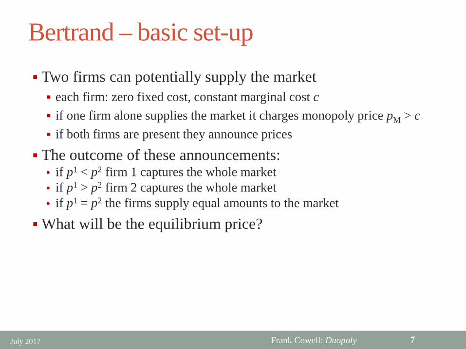
Bertrand – basic set-up Two firms can potentially supply the market each firm: zero fixed cost, constant marginal cost c if one firm alone supplies the market it charges monopoly price pM > c if both firms are present they announce prices

The outcome of these announcements:• if p1 < p2 firm 1 captures the whole market• if p1 > p2 firm 2 captures the whole market• if p1 = p2 the firms supply equal amounts to the market

What will be the equilibrium price?

July 2017 7


Bertrand – best response? Consider firm 1’s response to firm 2 If firm 2 foolishly sets a price p2 above pM then it sells zero output

• firm 1 can safely set monopoly price pM

If firm 2 sets p2 above c but less than or equal to pM then:• firm 1 can “undercut” and capture the market• firm 1 sets p1 = p2 − δ, where δ >0• firm 1’s profit always increases if δ is made smaller• but to capture the market the discount δ must be positive!• so strictly speaking there’s no best response for firm 1

If firm 2 sets price equal to c then firm 1 cannot undercut• firm 1 also sets price equal to c

If firm 2 sets a price below c it would make a loss• firm 1 would be crazy to match this price• if firm 1 sets p1 = c at least it won’t make a loss

Let’s look at the diagram

July 2017 8


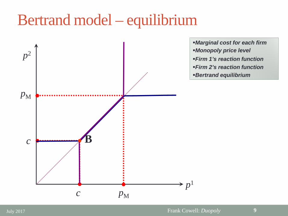
Bertrand model – equilibrium

July 2017 9

p2

c

c

p1

pM

pM

Firm 1’s reaction functionMonopoly price levelMarginal cost for each firm

Firm 2’s reaction functionBertrand equilibrium

B


Bertrand − assessment Using “natural tools” – prices Yields a remarkable conclusion

• mimics the outcome of perfect competition• price = MC

But it is based on a special case• neglects some important practical features• fixed costs• product diversity• capacity constraints

Outcome of price-competition models usually sensitive to these

July 2017 10


Overview

July 2017 11

Background

Price competition

Quantitycompetition

Assessment

Duopoly

The link with monopoly and an introduction to two simple “competitive” paradigms

•Collusion•The Cournot model•Leader-Follower


Quantity modelsNow take output quantity as the firms’ choice variable Price is determined by the market once total quantity is known:

• an auctioneer?

Three important possibilities:1. Collusion:

• competition is an illusion• monopoly by another name• but a useful reference point for other cases

2. Simultaneous-move competing in quantities:• complementary approach to the Bertrand-price model

3. Leader-follower (sequential) competing in quantities

July 2017 12


Collusion – basic set-up Two firms agree to maximise joint profits

• what they can make by acting as though they were a single firm• essentially a monopoly with two plants

They also agree on a rule for dividing the profits• could be (but need not be) equal shares

In principle these two issues are separate

July 2017 13


The profit frontier To show what is possible for the firms

• draw the profit frontier

Show the possible combination of profits for the two firms• given demand conditions• given cost function

Distinguish two cases1. where cash transfers between the firms are not possible2. where cash transfers are possible

July 2017 14


Frontier – non-transferable profits

July 2017 15

Π1

Π2 Constant returns to scaleDRTS (1): MC always rising

IRTS (fixed cost and constant MC)

Take case of identical firms

DRTS (2): capacity constraints


Frontier – transferable profits

July 2017 16

Π1

Π2Now suppose firms can make “side-payments”Increasing returns to scale (without transfers)

Profits if everything were produced by firm 1

ΠM

Profits if everything were produced by firm 2

•

•ΠM

The profit frontier if transfers are possibleJoint-profit maximisation with equal shares

ΠJ

ΠJ

Side payments mean profits can be transferred between firms

Cash transfers “convexify” the set of attainable profits


Collusion – simple model

July 2017 17

Take the special case of the “linear” model where marginal costs are identical:

c1 = c2 = c Will both firms produce a positive output?

1. if unlimited output is possible then only one firm needs to incur the fixed cost • in other words a true monopoly

2. but if there are capacity constraints then both firms may need to produce• both firms incur fixed costs

We examine both cases – capacity constraints first


If both firms are active total profit is[a – bq] q – [C0

1 + C02 + cq]

Maximising this, we get the FOC:a – 2bq – c = 0

Which gives equilibrium quantity and price: a – c a + c

q = –––– ; p = ––––2b 2 So maximised profits are:

[a – c]2ΠM = ––––– – [C0

1 + C02 ] 4b

Now assume the firms are identical: C01 = C0

2 = C0 Given equal division of profits each firm’s payoff is

[a – c]2ΠJ = ––––– – C08b

Collusion: capacity constraints

July 2017 18


Collusion: no capacity constraints

July 2017 19

With no capacity limits and constant marginal costs• seems to be no reason for both firms to be active

Only need to incur one lot of fixed costs C0• C0 is the smaller of the two firms’ fixed costs• previous analysis only needs slight tweaking• modify formula for PJ by replacing C0 with ½C0

But is the division of the profits still implementable?


Overview

July 2017 20

Background

Price competition

Quantitycompetition

Assessment

Duopoly

Simultaneous move “competition” in quantities



Cournot – basic set-up Two firms

• assumed to be profit-maximisers• each is fully described by its cost function

Price of output determined by demand• determinate market demand curve• known to both firms

Each chooses the quantity of output• single homogeneous output• neither firm knows the other’s decision when making its own

Each firm makes an assumption about the other’s decision• firm 1 assumes firm 2’s output to be given number• likewise for firm 2

How do we find an equilibrium?

July 2017 21


Cournot – model setup Two firms labelled f = 1,2 Firm f produces output qf

So total output is: • q = q1 + q2

Market price is given by:• p = p (q)

Firm f has cost function Cf(·) So profit for firm f is:

• p(q) qf – Cf(qf ) Each firm’s profit depends on the other firm’s output

• (because p depends on total q)

July 2017 22


Cournot – firm’s maximisation Firm 1’s problem is to choose q1 so as to maximiseΠ1(q1; q2) := p (q1 + q2) q1 – C1 (q1)

Differentiate Π1 to find FOC:∂Π1(q1; q2)

————— = pq(q1 + q2) q1 + p(q1 + q2) – Cq1(q1)

∂ q1

• for an interior solution this is zero Solving, we find q1 as a function of q2

This gives us 1’s reaction function, χ1 :q1 = χ1 (q2)

Let’s look at it graphically

July 2017 23


Cournot – the reaction function

July 2017 24

q1

q2

χ1(·)

•• Π1(q1; q2) = const

Π1(q1; q2) = const

Π1(q1; q2) = const

q0

Firm 1’s choice given that 2 chooses output q0

•

Firm 1’s Iso-profit curvesAssuming 2’s output constant at q0

firm 1 maximises profit

The reaction function

If 2’s output were constant at a higher level 2’s output at a yet higher level


χ1(·) encapsulates profit-maximisation by firm 1 Gives firm’s reaction 1 to fixed output level of competitor:

• q1 = χ1 (q2)

Of course firm 2’s problem is solved in the same way We get q2 as a function of q1 :

• q2 = χ2 (q1)

Treat the above as a pair of simultaneous equations Solution is a pair of numbers (qC

1 , qC2)

• So we have qC1 = χ1(χ2(qC

1)) for firm 1• and qC

2 = χ2(χ1(qC2)) for firm 2

This gives the Cournot-Nash equilibrium outputs

Cournot – solving the model

July 2017 25


Cournot-Nash equilibrium (1)

July 2017 26

q1

q2

χ2(·)

Firm 2’s Iso-profit curvesIf 1’s output is q0 ……firm 2 maximises profit

Firm 2’s reaction function

•• •

Repeat at higher levels of 1’s output

Π2(q2; q1) = constΠ1(q2; q1) = const

Π2(q2; q1) = const

q0

Firm 2’s choice given that 1 chooses output q0

χ1(·) Combine with firm ’s reaction function“Consistent conjectures”

C


q1

q2

χ2(·)

χ1(·)

0

(qC, qC)1 2

(qJ, qJ)1 2

Cournot-Nash equilibrium (2)

July 2017 27

Firm 2’s Iso-profit curves

Firm 2’s reaction functionCournot-Nash equilibrium


Firm 1’s reaction function

Outputs with higher profits for both firmsJoint profit-maximising solution


The Cournot-Nash equilibrium

July 2017 28

Why “Cournot-Nash” ? It is the general form of Cournot’s (1838) solution It also is the Nash equilibrium of a simple quantity game:

• players are the two firms• moves are simultaneous• strategies are actions – the choice of output levels• functions give the best-response of each firm to the other’s

strategy (action)

To see more, take a simplified example


Cournot – a “linear” example Take the case where the inverse demand function is:

p = β0 – βqAnd the cost function for f is given by:

Cf(qf ) = C0f + cf qf

So profits for firm f are:[β0 – βq ] qf – [C0

f + cf qf ] Suppose firm 1’s profits are Π Then, rearranging, the iso-profit curve for firm 1 is:

β0 – c1 C01 + Π

q2 = ——— – q1 – ————β β q1

July 2017 29


{ }

Cournot – solving the linear example Firm 1’s profits are given by Π1(q1; q2) = [β0 – βq] q1 – [C0

1 + c1q1]

So, choose q1 so as to maximise this Differentiating we get:

∂Π1(q1; q2) ————— = – 2βq1 + β0 – βq2 – c1

∂ q1

FOC for an interior solution (q1 > 0) sets this equal to zero Doing this and rearranging, we get the reaction function:

β0 – c1

q1 = max —— – ½ q2 , 02β

July 2017 30


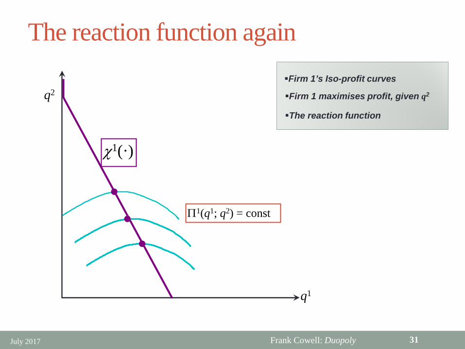
The reaction function again

July 2017 31

q1

q2

χ1(·)


Firm 1 maximises profit, given q2

The reaction function

••

•Π1(q1; q2) = const


Finding Cournot-Nash equilibrium

July 2017 32

Assume output of both firm 1 and firm 2 is positive Reaction functions of the firms, χ1(·), χ2(·) are given by:

a – c1 a – c2q1 = –––– – ½q2 ; q2 = –––– – ½q1

2b 2b Substitute from χ2 into χ1:

1 a – c1 ┌ a – c2 1 ┐

qC = –––– – ½ │ –––– – ½qC │ 2b └ 2b ┘

Solving this we get the Cournot-Nash output for firm 1:1 a + c2 – 2c1

qC = ––––––––––3b By symmetry get the Cournot-Nash output for firm 2:

2 a + c1 – 2c2 qC = ––––––––––3b


Take the case where the firms are identical• useful but very special

Use the previous formula for the Cournot-Nash outputs1 a + c2 – 2c1

2 a + c1 – 2c2 qC = –––––––––– ; qC = ––––––––––3b 3b

Put c1 = c2 = c. Then we find qC1 = qC

2 = qC where a – c

qC = ––––––3b From the demand curve the price in this case is ⅓[a+2c] Profits are

[a – c]2ΠC = –––––– – C09b

Cournot – identical firms

July 2017 33

Reminder


C

Symmetric Cournot

July 2017 34

q1

q2

qC

qC

χ2(·)

χ1(·)

A case with identical firmsFirm 1’s reaction to firm 2

The Cournot-Nash equilibriumFirm 2’s reaction to firm 1


Cournot − assessment Cournot-Nash outcome straightforward

• usually have continuous reaction functions

Apparently “suboptimal” from the selfish point of view of the firms• could get higher profits for all firms by collusion

Unsatisfactory aspect is that price emerges as a “by-product”• contrast with Bertrand model

Absence of time in the model may be unsatisfactory

July 2017 35


Overview

July 2017 36

Background

Price competition

Quantitycompetition

Assessment

Duopoly

Sequential “competition” in quantities



Leader-Follower – basic set-up Two firms choose the quantity of output

• single homogeneous output

Both firms know the market demand curve But firm 1 is able to choose first

• It announces an output level

Firm 2 then moves, knowing the announced output of firm 1 Firm 1 knows the reaction function of firm 2 So it can use firm 2’s reaction as a “menu” for choosing its own

output

July 2017 37


Firm 1 (the leader) knows firm 2’s reaction• if firm 1 produces q1 then firm 2 produces c2(q1)

Firm 1 uses χ2 as a feasibility constraint for its own action Building in this constraint, firm 1’s profits are given by

p(q1 + χ2(q1)) q1 – C1 (q1) In the “linear” case firm 2’s reaction function is

a – c2q2 = –––– – ½q1

2b So firm 1’s profits are

[a – b [q1 + [a – c2]/2b – ½q1]]q1 – [C01 + c1q1]

Leader-follower – model

July 2017 38

Reminder


Solving the leader-follower model

July 2017 39

Simplifying the expression for firm 1’s profits we have: ½ [a + c2 – bq1] q1 – [C0

1 + c1q1] The FOC for maximising this is:

½ [a + c2] – bq1 – c1 = 0 Solving for q1 we get:

1 a + c2 – 2c1 qS = ––––––––––2b

Using 2’s reaction function to find q2 we get:2 a + 2c1 – 3c2

qS = ––––––––––4b


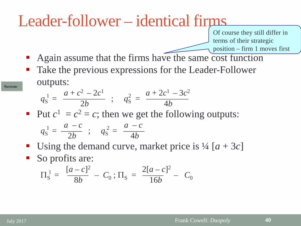
Leader-follower – identical firms

July 2017 40

Again assume that the firms have the same cost function Take the previous expressions for the Leader-Follower

outputs:1 a + c2 – 2c1

2 a + 2c1 – 3c2 qS = –––––––––– ; qS = ––––––––––2b 4b

Put c1 = c2 = c; then we get the following outputs:1 a – c 2 a – c

qS = ––––– ; qS = –––––2b 4b Using the demand curve, market price is ¼ [a + 3c] So profits are:

1 [a – c]2 2[a – c]2 ΠS = ––––– – C0 ; ΠS = ––––– – C08b 16b

Reminder

Of course they still differ in terms of their strategic position – firm 1 moves first


qS1

C

Leader-Follower

July 2017 41

q1

q2

qS2 S

Firm 1’s Iso-profit curvesFirm 2’s reaction to firm 1Firm 1 takes this as an opportunity setand maximises profit hereFirm 2 follows suit

Leader has higher output (and follower less) than in Cournot-Nash “S” stands for von Stackelberg

χ2(·)


Overview

July 2017 42

Background

Price competition

Quantitycompetition

Assessment

Duopoly

How the simple price- and quantity-models compare


Comparing the models The price-competition model may seem more “natural” But the outcome (p = MC) is surely at variance with everyday

experience To evaluate the quantity-based models we need to:

• compare the quantity outcomes of the three versions• compare the profits attained in each case

July 2017 43


J

qM

C S

Output under different regimes

July 2017 44

qM

qCqJ

qC

qJ

q1

q2

Joint-profit maximisation with equal outputs

Reaction curves for the two firms

Cournot-Nash equilibrium

Leader-follower (Stackelberg) equilibrium


Profits under different regimes

July 2017 45

Π1

Π2

ΠM•

•ΠM

Joint-profit maximisation with equal shares

ΠJ

ΠJ

Attainable set with transferable profits

• J• .

C

Profits at Cournot-Nash equilibriumProfits in leader-follower (Stackelberg) equilibrium

• S

Cournot and leader-follower models yield profit levels inside the frontier


What next? Introduce the possibility of entryGeneral models of oligopolyDynamic versions of Cournot competition

July 2017 46

DUOPOLY - London School of Economicsdarp.lse.ac.uk/presentations/MP2Book/OUP/Duopoly.pdf · Frank...

Documents

Transcript of DUOPOLY - London School of Economicsdarp.lse.ac.uk/presentations/MP2Book/OUP/Duopoly.pdf · Frank...