Ductility and Failure Modes of Single Reinforced Concrete...
24
Ductility and Failure Modes of Single Reinforced Concrete Columns Hiromichi Yoshikawa 1 and Toshiaki Miyagi 2 Key Words: seismic capacity design, reinforced concrete column, failure modes, deformational ductility, flexural failure, shear failure, shear failure after flexural yielding, shear-degrading curve, nonlinear dynamic analysis, random deformation history 1 Dept. of Civil Engrg., Musashi Inst. of Tech., Tokyo, Japan. 2 Inst. of Tech., Tokyu Construction Co., Sagamihara-City, Japan.
Transcript of Ductility and Failure Modes of Single Reinforced Concrete...

Ductility and Failure Modes of Single Reinforced Concrete Columns
Hiromichi Yoshikawa1 and Toshiaki Miyagi2
Key Words:
seismic capacity design, reinforced concrete column,
failure modes, deformational ductility, flexural failure, shear failure, shear failure after flexural yielding, shear-degrading curve, nonlinear dynamic analysis, random deformation history
1 Dept. of Civil Engrg., Musashi Inst. of Tech., Tokyo, Japan. 2 Inst. of Tech., Tokyu Construction Co., Sagamihara-City, Japan.
Ductility and Failure Modes
of Single Reinforced Concrete Columns
Hiromichi Yoshikawa3 and Toshiaki Miyagi4
Abstract
The main purpose of the seismic analysis of structures is to assess the level of risk
associated with loss of serviceability, restorability and collapse. With regard to a reinforced
concrete bridge column, it is extremely important to identify failure modes and to qualify the
deformational ductility from the point of the capacity design methodology (Paulay and
Priestley (1992)).
In this paper, types of failures of single reinforced concrete columns are classified as
flexural failure, shear failure after yielding of longitudinal reinforcement, and shear failure.
Procedures to determine failure modes are presented by comparing δ−P curve (push-over
behavior) and the degrading capacity of shear strength along the deformational history.
Nonlinear dynamic analysis is also carried out for reinforced concrete columns
3 Dept. of Civil Engrg., Musashi Inst. of Tech., Tokyo, Japan. 4 Inst. of Tech., Tokyu Construction Co., Sagamihara-City, Japan.

subjected to the recorded time history of strong seismic actions. The shear-degrading curve
proposed by Priestley et al. (1996) is extended to a case of random deformation history to
cope with actual seismic excitation. The proposed method is compared with data of
experimental works and numerical simulations are carried out.
Introduction
Seismic capacity of a substructure supporting superstructure is examined
by comparing response values (load or deformation) by earthquake motion with its strength or ductility in many cases. For example, comparison of response
deformation and ductility performance of a structural system is a typical technique of seismic capacity assessment. Both these works are usually performed separately during a design procedure. However, this is not considered to be a rational method, especially in cases where seismic actions and structural ductility
are affected to each other during a strong earthquake. When considering reinforced concrete structures, it is important to clearly
define a failure mode and to appropriately assess the seismic capacity for each
failure mode. Flexural failure and shear failure for reinforced concrete bridge columns can be easily judged. However, a failure mode in-between these (“shear failure after flexural yielding”) is still open to question and often become critical in seismic design (AIJ Design Guidelines (1990), An and Maekawa (1998)).
In this study, three failure modes of a single reinforced concrete column
are defined, and identification methods in static analyses and assessment methods for ductility factors are proposed. Furthermore, comparison with test results and
numerical simulations were performed. A particular discussion focuses on a degradation model of shear strength accompanying large repeated deformation far beyond the yield point of the main reinforcement.
The degradation shear model in dynamic random response is proposed and dynamic nonlinear analyses by spring mass model of a single degree-of-freedom are carried out. The degradation process of structural members during the time history is assessed based on an amount of damage accumulated, then

determination of failure/non-failure as well as failure modes are made, and finally the maximum response displacement is computed. Numerical simulations for
actual bridges were performed, which offer useful and interesting information.
Classification of Failure Modes of Single Reinforced Concrete Columns
Now we consider the classification and definition of failure modes of single type of reinforced concrete bridge column subjected to large cyclic deformation. We firstly consider increased cyclic tests of displacement control
type as shown in Figure 1, and define yδ at the displacement when longitudinal
reinforcement yields and muδ at the displacement of ultimate flexural failure on
the envelope curve ( δ−P curve).
The shear strength is, on the other hand, gradually reduced due to large cyclic deformation beyond the displacement of yielding of the main reinforcement. The shear strength are thus denoted as:
yoV : initial shear strength
ykV : degrading shear strength due to cyclic loading

Figure 1. upper: Cyclic Behavior of Single Reinforced Concrete Column, lower: Classification of Failure Modes
Now that the failure modes can be defined according to the intersecting
relationship between the δ−P curve and the degrading shear capacity envelope (Priestley et al. (1996)). This is
A) Shear failure: Shear failure occurs before the main reinforcement yields B) Shear failure after flexural yielding: Shear failure occurs after the main reinforcement yielding
C) Flexural failure: The δ−P curve and the degrading shear capacity envelope do not intersect till reaching the ultimate flexural point ( muδδ = ).
Photo 1. exhibits examples of test specimens failed in each of these failure
displacement δ
load
P
longitudinalreinforcementyielded
ductilityfcctor
1 μmu
ultimate
(B) shear failure after yilding
δy δmu
P
δy δmu
(A) shear failure
degradation ofshear strength curve
envelope curve(P- δ curve)
(C) flexural failure
δy δmu

modes. The type A failure is caused when an excessive quantity of the main reinforcement is arranged or when a quant ity of lateral reinforcement is
insufficient, and it has been pointed out that this failure type extremely deteriorates seismic performance. On the other hand, the type C failure means that shear failure does not occur under any excessive input of earthquake motion, and that full ductile performance is maintained. The type B failure (flexural shear
failure) located between those types shows the limited ductile shear strength leading to being critical concerning seismic design.
When we define a member ductility ratio µ as δµ = / yδ , the three
failure types defined in Figure 1 are classified as follows:
A) shear failure : 1<µ B) shear failure after yielding : muµµ <<1
(1) C) flexural failure : muµµ=
shear failure(C05) shear failure after yielding(C10) flexural
failure(C20)
Photo 1. Test Examples for Three Failure Modes (Hattori et al. 1998)

Static Nonlinear Analysis and Shear Strength
Deformational Analysis
We will perform deformational analyses of single reinforced columns to
obtain δ−P curves. The lateral displacement δ includes contributions of
flexural deformation flexδ , shear deformation shearδ and rotating displacement
pulloutδ caused by pulling out the main reinforcement at the column base. Namely,
pulloutshearflex δδδδ ++= (2)
As analytical conditions for materials, a model was applied as the concrete
constitutive law in which a confining effect by lateral reinforcement is reflected, and the constitutive law of longitudinal reinforcement was assumed to be the tri- linear type model. Shear deformation shearδ was neglected in the present study.
We assumed that plastic hinge is formed in the zone from the column base to 1.0d (d is an effective height of column cross-section). The rotating displacement
pulloutδ caused by pulling out the main reinforcement was calculated by applying
the conventional equation.
Shear Strength by Modified Truss Analogy
The well-known modified truss analogy was applied for the calculation of
shear strength in this study. This means that shear strength is obtained by summing shear strength by lateral reinforcement sV and strength of concrete shear resisting mechanisms cV (for example, JSCE Specification (1996)). In this
paper, the following expressions are used to consider initial shear strength and degrading shear strength separately.

initial shear strength : 00 csy VVV +=
(3-a)
degrading shear strength due to cyclic loading: cksyk VVV +=
(3-b)
The shear strength by lateral reinforcement sV is calculated based on the truss
analogy by the following equation:
szfAV wyws /cotθ=
(4)
In which wA is the total area of shear reinforcement arranged in spacing
s , and θ is a compressive strut angle.
It has been pointed out that the reduction of shear strength accompanying
cyclic excessive deformation is caused by degradation of the component of concrete contribution 0cV . The symbol ckV is used as the strength in the
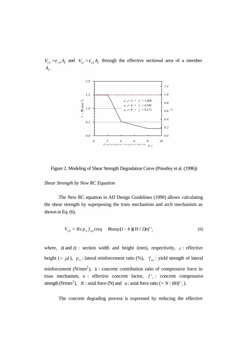
degradation process. Here we introduce the degradation curve proposed by Priestley et al. (1996) as shown in Figure 2.
In Figure 2, the left vertical axis represents the shear strength cτ , the right
vertical axis the shear degradation factor ζ obtained by dividing shear strength
ckV by the initial shear strength 0cV . The initial value of this degradation factor
ζ is equal to 1, and 1<ζ for the larger deformation which is expressed such that )( dµζζ = . Thus, the relationship between the initial shear strength 0cτ and the degrading shear strength ckτ as well as between 0cV and ckV are simply
written as
0cck VV ζ= , 0cck ζττ = (5)
In Eq. (5), both of shear strengths 0cV and 0cτ can be related such as
ecc AV 00 τ= and eckck AV τ= through the effective sectional area of a member
eA .
Figure 2. Modeling of Shear Strength Degradation Curve (Priestley et al. (1996))
Shear Strength by New RC Equation
The New RC equation in AIJ Design Guidelines (1990) allows calculating the shear strength by superposing the truss mechanism and arch mechanism as
shown in Eq. (6).
cwywy fHBfpzBV ')/)(( νβθθ 21tancot0 −+= (6)
where, B and H : section width and height (mm), respectively, z : effective
height ( jd= ), wp : lateral reinforcement ratio (%), wyf : yield strength of lateral
reinforcement (N/mm2), β : concrete contribution ratio of compressive force in truss mechanism, ν : effective concrete factor, cf ' : concrete compressive strength (N/mm2), N : axial force (N) and n : axial force ratio ( cBHfN '/= ).
The concrete degrading process is expressed by reducing the effective
0.0
0.5
1.0
1.5
2.0
0 2 4 6 8 10d i s p l a c e m e n t r e s p o n s e f a c t o r μd
τc(
N/m
m2 )
0.0
0.2
0.4
0.6
0.8
1.0
1.2
ζ
μd= 2 → ζ= 1.000
μd= 4 → ζ= 0.345
μd= 8 → ζ= 0.172
concrete factor ν and an angle of concrete compressive struts in the truss
mechanism as a single function of rotating angle pR in the plastic hinge zone of
column base. This proposed formula reflects the new theoretical consideration to be proven by a wide range of experimental database). Comparison with Test Results and Numerical Simulation
Comparison with Test Results
In order to verify the validity of this proposed technique, we compare
analytical results with loading test results using three specimens referred to as C05, C10 and C20 (Hattori et al. (1998)). Each specimen having cross-sectional dimensions of 320 mm×320 mm and a shear span ratio of 4.05 were designed to
arrange reinforcements for the above-mentioned three types of failure mode (see
Photo 1 again). The analytical result of specimen C05 by the proposed method shows that
deformational behavior is quite similar to the test result and predicted the shear
failure identical to the test. The analytical results of specimen C10 using two shear strength degradation curves intersected nearly at the same points on δ−P envelop curve, and coincided with the failure mode of the test results (shear failure after flexural yielding). The analysis of specimen C20 shows that both of
the shear degrading curves do not intersect with δ−P curve and the failure mode is assessed to be of the flexural failure.
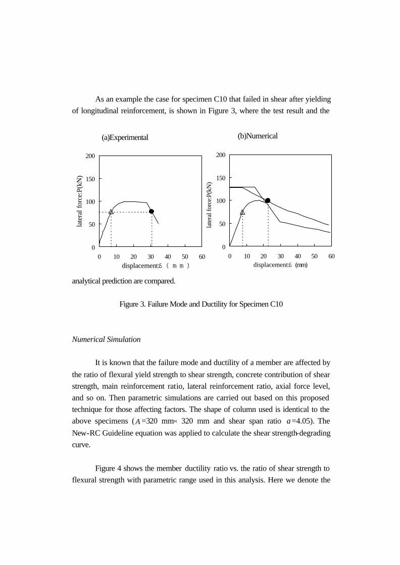
As an example the case for specimen C10 that failed in shear after yielding of longitudinal reinforcement, is shown in Figure 3, where the test result and the
analytical prediction are compared.
Figure 3. Failure Mode and Ductility for Specimen C10
Numerical Simulation
It is known that the failure mode and ductility of a member are affected by
the ratio of flexural yield strength to shear strength, concrete contribution of shear strength, main reinforcement ratio, lateral reinforcement ratio, axial force level, and so on. Then parametric simulations are carried out based on this proposed technique for those affecting factors. The shape of column used is identical to the above specimens (A =320 mm×320 mm and shear span ratio a=4.05). The
New-RC Guideline equation was applied to calculate the shear strength-degrading curve.
Figure 4 shows the member ductility ratio vs. the ratio of shear strength to flexural strength with parametric range used in this analysis. Here we denote the
(a)Experimental
0
50
100
150
200
0 10 20 30 40 50 60displacement:δ(mm)
late
ral f
orce
:P(k
N)
(b)Numerical
0
50
100
150
200
0 10 20 30 40 50 60displacement:δ(mm)
late
ral f
orce
:P(k
N)

ratio of shear strength to flexural strength as muy VV /0 (flexural capacity muV of
column obtained by dividing the ultimate flexural moment muM at the column
base by the shear span a ). It can be seen that the failure mode shifts from flexural to shear mode and ductility factor of columns decreases, as the ratio of shear strength to flexural strength becomes smaller.
From this figure, it may be suggested that each failure mode can be
approximately estimated by the ratio of shear strength to flexural strength in such a way that
Shear failure: ratio of shear strength to flexural strength<0.8 Shear failure after yielding of longitudinal reinforcement:
0.8<ratio of shear strength to flexural strength<1.5
Flexural failure: 1.5<ratio of shear strength to flexural strength
Figure 5 illustrates relationship among the main reinforcement ratio, the lateral reinforcement ratio and the member ductility factor for two axial force
levels. This figure implies that with increase of the axial force applied to the member, its ductility factor becomes lower and the failure mode tends to shift from the flexural to the shear mode.

(a)σo/f’c=0 (b) σ
o/f’c=0.2
Figure 5. Evaluation of Failure Modes and Ductility Ratios for Two Axial Level
in Relation of Main/Shear Reinforcement Ratio
Failure and Shear Degradation in Dynamic Random Process Classification of Failure Modes in Random Process
Now we consider an expansion of the proposed method to random response of concrete columns subjected to a seismic load shown in Figure 6, illustrating dynamic nonlinear response. FIGURE 6 schematically depicts the time history response for (a) curvature at column base, (b) lateral force acting on the
column base and (c) lateral displacement at column top. Figure (b) describes that
0.80.6
0.40.2
0.020.04
0.060.08
2
4
6
8
10
shear reinf. ratio : pw・fwy/f'cducti
lity
fa
cto
r :
μ
main
reinf.
ratio
: ps
・fsy
/f'c
0.80.6
0.40.2
0.020.04
0.060.08
2
4
6
8
10
shear reinf. ratio : pw・fwy/f'c
ductility
factor
:
μ
main
rein
f. ra
tio
: ps・
fsy/
f'c
0.2 0.3 0.4 0.5 0.6 0.7 0.8 0.90.01
0.02
0.03
0.04
0.05
0.06
0.07
0.08
main reinf. ratio : ps・fsy/f'c
shea
r re
inf. r
atio
: p
w・f
wy/
f'c
0.2 0.3 0.4 0.5 0.6 0.7 0.8 0.90.01
0.02
0.03
0.04
0.05
0.06
0.07
0.08
main reinf. ratio : ps・fsy/f'c
shea
r re
inf. r
atio
: p
w・f
wy/
f'c

the damage at the base, where curvature at base exceeds the displacement of the main reinforcement yielding, results in gradual reduction of shear strength and
finally shear failure occurs at the time when the peak amplitude of the lateral force exceeds the shear strength (shear failure after flexural yield). On the other hand, Figure (c) indicates that flexural failure may occur because lateral displacement δ reaches the ultimate flexural displacement muδ .
(a)
(b)
(c)
Figure 6. (a) Curvature at Column Base, (b) Lateral Force Acting on Column Base and (c) Lateral Displacement at Column Top in Time History
Response
curv
atur
e at
colu
mn
base
time
disp
lace
men
t at
colu
mn
top
flexural failure
+δmu
Vy1 Vy0
Vy2
degrading shear strength :Vyk(t)
shear failure
V(t)
late
ral f
orce
+φy
-φy
-δmu
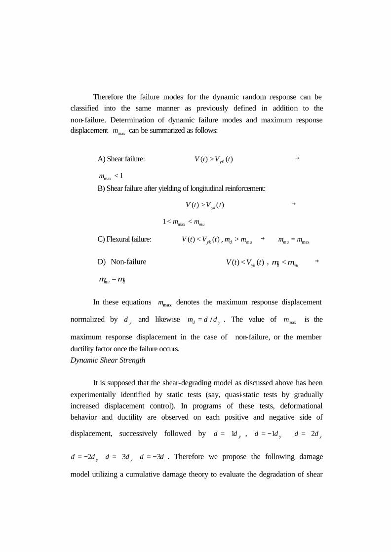
Therefore the failure modes for the dynamic random response can be classified into the same manner as previously defined in addition to the
non-failure. Determination of dynamic failure modes and maximum response displacement maxµ can be summarized as follows:
A) Shear failure: )()( 0 tVtV y> →
1max <µ
B) Shear failure after yielding of longitudinal reinforcement:
)()( tVtV yk> →
muµµ << max1
C) Flexural failure: )()( tVtV yk< , mud µµ > → maxµµ =mu
D) Non-failure )()( tVtV yk< , mud µµ < →
dmu µµ =
In these equations maxµ denotes the maximum response displacement
normalized by yδ and likewise yd δδµ /= . The value of maxµ is the
maximum response displacement in the case of non-failure, or the member
ductility factor once the failure occurs. Dynamic Shear Strength
It is supposed that the shear-degrading model as discussed above has been
experimentally identified by static tests (say, quasi-static tests by gradually increased displacement control). In programs of these tests, deformational behavior and ductility are observed on each positive and negative side of
displacement, successively followed by yδδ 1+= , yδδ 1−= yδδ 2+=
yδδ 2−= yδδ 3+= δδ 3−= . Therefore we propose the following damage
model utilizing a cumulative damage theory to evaluate the degradation of shear

strength during the dynamic random process. As shown in Figure 7, a factorξ is newly introduced in order to express
the degradation of shear strength when a column is damaged by a single attack in earthquake wave. The original degrading factor ζ shown in Figure 2 is modified
by multiplying a factor m in the form
2<dµ : 1=ξ
42 <≤ dµ : 1655.03275.0 ++−= mm dµξ
84 <≤ dµ : 1518.004325.0 +−−= mm dµξ
dµ≤8 : 1828.0 +−= dmµξ (7)
The modification factor m is supposed to be in a range of 10 << m , and
),( dm µξξ = is referred to as the degrading factor due to a single attack, which is different from the standard degrading curve )( dµξξ = . Here in the present paper,
the factor m is assumed to be 0.5 as a constant value through the degradation process.
By sequentially numbering suffix i for large deformation amplitude δ
(here in this study yδδ 2|| > ) as ki ,...,3,2,1= and designating as kξξξξ ,...,,, 321 ,
the following equation of sequential multiplication leads to the factor kς .
∏=
==k
iikk
1321 ... ξξξξξζ
(8)
During seismic motion concrete contributions of shear strength ckckV τ,
are updated using the degrading factor kζ obtained from Eq. (8).
μ

Figure 7. Degradation Factors for (a) Increased Displacement Control
and (b) Random Response Displacement
Nonlinear Dynamic Analysis
Dynamic Failure Analysis of Bridge Columns
In this section numerical simulation is performed on a single type of bridge column that was heavily damaged in the Hyogo-Ken Nambu Earthquake. Specifications of cross-sections and calculated properties of members used for simulation are listed in Table 1. Three members are designated as
time
+4
1
+4δy
+3δy +2δy
0 1
ζ,ξ
μ
1
m
ζ=ζ(μ)
μ
ζ
ξ i=1
2
3 1
μ
2
time
3
ζ
+4
-2 -4
0
μ
-2 -4
0
0 1
(a)
(b)
i=1,2,3・・・,k:sequential peak number
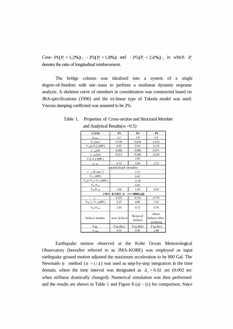
Case- %).( 211 =tPP , - %).( 813 =tPP and - %).( 425 =tPP , in which tP
denotes the ratio of longitudinal reinforcement.
The bridge column was idealized into a system of a single
degree-of- freedom with one-mass to perform a nonlinear dynamic response analysis. A skeleton curve of members in consideration was constructed based on
JRA-specifications (1996) and the tri- linear type of Takeda model was used. Viscous damping coefficient was assumed to be 2%.
Table 1. Properties of Cross-section and Structural Member
and Analytical Results(m =0.5)
Earthquake motion observed at the Kobe Ocean Meteorological
Observatory (hereafter referred to as JMA-KOBE) was employed as input earthquake ground motion adjusted the maximum acceleration to be 800 Gal. The Newmark- β method ( 4/1=β ) was used as step-by-step integration in the time domain, where the time interval was designated as 02.0=∆ t sec (0.002 sec
when stiffness drastically changed). Numerical simulation was then performed and the results are shown in Table 1 and Figure 8 (a) - (c) for comparison. Since
CASE P1 P3 P5p t(%) 1.2 1.8 2.4
T y (sec) 0.749 0.630 0.553V mu[=Pu] (MN ) 6.91 9.54 12.35
δy (m) 0.066 0.068 0.071
δmu (m) 0.312 0.268 0.224
V s[=S s] (MN )
μmu 4.72 3.94 3.15
τco (N /mm2)
Vco (MN )
Vyo[=V co+V s ] (MN )
Vco/V yo
Vyo/V mu 1.66 1.20 0.93
ζ 0.553 0.514 0.775Vck=ζV co (MN ) 5.23 4.86 7.32
Fig. Fig.8(a) Fig.8(b) Fig.8(c)μmax 4.31 3.94 2.68
failure modes non failure flexuralfailure
shearfailure after
yielding
11.45
0.83
Vyk/V mu 1.05 0.72 0.76
J M A - K O B E (α max=800Gal)
2.00
a n a l y t i c a l r e s u l t s
9.45
1.51

μμ
μ
the seismic input data is based on the Hyogo-Ken Nambu Earthquake, the extremely large excitation has completed in the first 20 sec., and that the failure or non-failure was determined during the time of 5=t ~10 sec in all cases.
Case-P1 of Figure 8 shows that several large deformations over 2=dµ
lead to reducing the shear degrading factor up to 558.0=kζ , however neither shear failure nor flexural failure occurred after all (non-failure: 31.4max =µ ). On
the other hand, Case-P3 in Figure (b) illustrates that lateral displacement reached the ultimate flexural ductility at the time of the initial large deformation ( mud µµ = ), causing a flexural failure ( =maxµ 3.94). It is interesting to see that the
degrading shear strength and the response lateral force intersected in the same amplitude. Case-P5 in Figure (c) implies a typical shear failure after flexural damage. Although the response displacement dµ was not large and then the
degradation of shear strength was limited to 783.0=kζ , the shear failure was
initiated when 16.9=t sec due to excessively large lateral force V (shear failure after flexural yielding: 67.2max =µ ).
In this manner, differences in dynamic failure modes and maximum
response displacements are clearly recognized because of the difference of static and dynamic character istics accompanying the difference of amount of the longitudinal reinforcement, though the earthquake excitation and the structural configuration are identical. It is also found in these three cases that ratios of shear
strength to flexural strength muy VV /0 are getting small in order of P1, P3 and P5
(see TABLE 1), and then the failure mode shifted from non-failure ( 31.4max =µ ),
flexural failure ( 943.max =µ ), and shear failure ( 67.2max =µ ).
Ratio of shear strength to flexural strength is expected to be useful to
determine the failure mode in the dynamic analysis. These analytical results mean that while the increase of longitudinal reinforcement improves the static loading
capacity, the dynamic seismic capacity may be sometimes affected adversely. It may be concluded that the columns analyzed are to be high strength but low seismic capacity.

TIME(sec)
V(V(
TIME(sec)
V(
(a)CASE-P1: (μmax=4.31) (b) CASE-P3: (μmax=3.94) (c)CASE-P5: (μmax=2.68) non-failure flexural failure shear failure after yielding
Figure 8. Time History Response of Lateral Displacement (upper) and Lateral Force (lower) under JMA-KOBE
( 800max =α Gal)
Numerical Simulation
Next we again employed earthquake motion of JMA-KOBE 1995, in which the maximum acceleration varied from 500 to 900 Gal and the contribution
sV due to the lateral reinforcement changed as 0.5,...,5.1,0.1,5.0,01.0=sV MN
so as to carry out nonlinear parametric dynamic analyses. Figure 9 and Figure 10 are examples of parametric simulations, taking focus on the degradation process of shear strength in time-histories
Figure 9 shows the degrading process of concrete contribution by the
6
4
2
0
-2
-4
-6
15
10
5
0
-5
-10
-15
μmu=3.94 μmu=4.72 μmu=3.15
no intersect
V(t)
flexural failure
t=6.50sec
t=6.52sec
degradation of shear strength Vyk(t)
V(t)
time (sec)
degradation of shear strength Vyk(t)
late
ral f
orce
V
disp
lace
men
tμd
no intersect
time (sec)
no intersect
shear failure after yielding

degrading factors ζ and ξ in 321 ,,=i , and the degrading process of concrete contribution (shear strength: ckV and shear strength: ckτ ) of the shear strength can be examined. It was found that the number of the large deformation for dµ 2≥ and the finally obtained kζ depend on the characteristics of the earthquake input motion as well as the structure configuration.
Figure 10 shows the degrading shear strength ckτ taking the maximum
ground acceleration as a parameter. It was found that, as the maximum input acceleration ( maxα : indicated in the figure) increases, the column causes the more damage to become the lower shear strength ckτ .
(a) (b)
Figure 9. (a) Relationship of Response Displacement and Degradation Factors kξ
and kζ , and (b) Response Displacement in The Time History
0
1
2
3
4
5
00.51ζ,ξ
μd
ξζ
JMA-KOBE(P3, αmax =800Gal )
0 5 10 15 20
time(sec)
i=1
3
2

Figure 10. Comparison of Degrading Shear Strength ckτ and Maximum
Deformation Response ratio dµ [ 2/27' mmNf c = → 2/51.1 mmNco =τ ]
Conclusions
Through the discussions so far we summarize the conclusion of this paper as follows:
Failure modes for a single reinforced concrete column were classified into three types: shear failure, shear failure after flexural yielding and flexural failure. It is especially difficult to model the shear failure after flexural yielding which has been discussed from the viewpoint of seismic design procedure. The modified
truss analogy incorporating concrete degrading models proposed by Priestley and New RC equation from AIJ Design Guidelines were utilized to predict the degrading process up to the shear failure.
Comparison of this proposed technique with the results of static loading tests using three specimens (increased displacement control test) indicated generally good agreement concerning the failure mode and displacement ductility. The analytical results by parametric simulation suggested usefulness of the ratio
of shear strength to flexural strength.
In order to apply this analytical technique to random responses of a
0.0
0.5
1.0
1.5
2.0
0 2 4 6 8 10μd
τc (N
/mm
2)
500Gal
600 700
800
ξ
ζ

column subjected to a seismic load, the concrete degrading model proposed by Priestley was modified in terms of the cumulative damage model. Furthermore, a
dynamic nonlinear response analysis was performed using one mass and single-degree-of- freedom model under recorded seismic action. Reduction of shear strength is updated in the time history, and it became possible to judge either failure or non-failure and to calculate the maximum displacement.
When maximum input acceleration was, for instance, 800max =α Gal,
degrading strength ckτ got lowered to 0.6 - 0.8 N/mm2 whereas initial shear
strength coτ of concrete was 1.5 N/mm2. On the other hand, the shear strength
ckτ for seismic design in the current Japanese specifications (JRA Specification
and JSCE Seismic Code) is approximately 0.3 - 0.5 N/mm2, which is found to be a more conservative value.
In this modeling, however, the more adequate determination of the factor is necessary, which has been examined in our laboratory by experimental works as well as by the analytical consideration.
Further numerical simulations, taking the quantity of main reinforcement, quantity of
lateral reinforcement, types of earthquakes and maximum acceleration as parameters, for
actual reinforcement concrete bridge columns need to be performed to obtain more
comprehensive numerical information.
References
An, X. and Maekawa, K. (1998). “Shear Resistance and Ductility of RC Columns after Yield
of Main Reinforcement.” Journal of Materials, Concrete Structures and Pavements, JSCE,
No.585/V-38, 233-247.
Architectural Institute of Japan (1990). Design guidelines for earthquake resistant reinforced
concrete buildings based on ultimate strength concept, Japan. (In Japanese)
Hattori, H., Miyagi, T., Masuda, Y., Iketani, K. and Yoshikawa, H. (1998). “Evaluation of
Failure Mode and Ductility of Reinforced Concrete Columns.” The 10th Japan Earthquake
Engineering Symposium, Proceedings Vol. 2, 2157-2162. (In Japanese)
Japan Society of Civil Engineers (1996). Standard specification for concrete structures,
Seismic Design, JSCE. (In Japanese)
Japan Road Association (1996). Specification for highway bridges, Part V:
Earthquake-resistant design. (In Japanese)
Paulay, T. and Priestley, M.J.N. (1992). Seismic Design of Reinforced Concrete and Masonry
Buildings, John Wiley & Sons.
Priestley, M.J.N., Seible, F., and Calvi. G.M. (1996). Seismic Design and Retrofit of Bridges,
John Wiley & Sons.