Institute for International Integration Studies

IIIS Discussion Paper

No.252 / June 2008

House Prices and Economic Risks - Are irish HouseholdsRational?

Dirk G. BaurDublin City University - Business School

Conor McKeating Dublin City University - Business School

IIIS Discussion Paper No. 252

House Prices and Economic Risks – Are Irish Households Rational? Dirk G. Baur Conor McKeating Disclaimer Any opinions expressed here are those of the author(s) and not those of the IIIS. All works posted here are owned and copyrighted by the author(s). Papers may only be downloaded for personal use only.

House Prices and Economic Risks -

Are Irish Households Rational?

Dirk G. Baur1

& Conor McKeating2

Dublin City University – Business School

First version: May 2008

Abstract

This study analyzes the evolution of house prices in Ireland and investigates the question of whether

Irish households are overexposed to certain economic risks rendering the decision to buy a house too

risky and hence irrational. We use a simple theoretical framework to demonstrate the investment

options of a typical household and derive the risk factors associated with the purchase of a house with

respect to other types of investment.

Irish households hold the majority of their investments in property, specifically in their own houses.

The empirical results illustrate that this wealth is exposed to inflation, interest rate changes and the

business cycle. This exposure, while not problematic in times of low interest rates, moderate inflation

and economic expansion, amplifies the risk to the value of households’ investments if inflation

increases, interest rates rise or the economy is in recession. We argue that the adoption of the euro has

increased this risk because interest rates are exogenous to the Irish economy which could lead to a

situation of deteriorating economic conditions and rising interest rates..

Our findings indicate that Irish households potentially underestimate the risk of buying a house.

Viewing the purchase of a house as a risky investment could help reduce private debt in the future.

JEL classification: D14, E30, E44

Keywords: house prices, economic risk, household investment decisions

1 Corresponding author. Address: DCU, Collins Avenue, Glasnevin, Dublin 9, Ireland, email: dirk.baur@dcu.ie 2 email: conor.mckeating@dcu.ie We thank Niels Schulze for helpful comments and conversations.

Introduction

In 1999, Ireland, along with 10 other members of the European Union, adopted the new single

European currency, the euro. Interest rates would now be set by the ECB, in accordance with

conditions in the euro area as a whole. Of the original members, Ireland made up 1.4% of the

euro area by GDP, and hence has very little influence over the level of official interest rates3.

Prior to adoption of the euro, the Irish Central Bank was forced to cut official interest rates by 3%

to bring Irish rates in line with those in Germany. However, this meant cutting rates aggressively

in a booming economy4 and gave rise to concerns about fuelling domestic inflation.

While consumer prices increased rapidly in the following 12 months, worries about domestic

inflation receded as price levels moderated thereafter (see Figure 1). However, lower interest

rates have come in tandem with an increase in personal debt. In 2005, Ireland had the second

highest GNP per capita5 in the OECD, but also the second highest level of mortgage debt per

capita6 (OECD 2006b). These debt levels mean Irish households are overly exposed to interest

rates, at a time when a concerted tightening cycle by the ECB has left many Irish households with

a sharply reduced disposable income and has put pressure on consumer spending, the property

market and with it tax receipts and the government’s fiscal situation.

From December 1999 to September 2007, private sector credit grew by 340% and household

mortgage debt by 389%. Much of this additional borrowed money has been invested in housing.

National Irish Bank (2008) showed Irish households have 67% of their investment portfolio in

property, of which 49% is in their own homes. This has been a highly profitable strategy when

house prices increased, but has exposure to interest rates, inflation and the business cycle at a

time when all are moving in directions which are unfavourable to Irish households. While

inflation and the business cycle have domestic drivers, interest rates are now an exogenous

variable in the Irish economy. The current issues in the credit markets did not precede the

downturn in the Irish housing market, but have brought into focus the unbalanced nature of Irish

household investment.

3 At December 2007, this figure was 2.1% 4 Real GNP growth in the period 1995-1998 averaged 8.1% per annum (Reuters Ecowin) 5 second to Luxembourg as of 2005 6 second to New Zealand as of 2005

2

Literature Review

In the period 1995-2005, real Irish house prices increased by over 200%, the largest increase in

the period in the OECD (OECD 2006a). Both the duration and the magnitude of real price

increases are unprecedented for Ireland and have coincided with the longest sustained period of

economic growth in Ireland’s history, with GNP increasing from 47.0bn to 135.7bn euros in the

same period (Reuters Ecowin), an average annual growth rate of 10.6%. However, in recent

years, the drivers of Irish GNP growth have switched from exports and FDI to consumption and

rising property valuations leaving Irish households’ investment portfolios overexposed to

property, primarily through their own homes. Private sector credit grew by 340% from December

1999 to September 2007. In the same period, household mortgage debt rose by 389%.

Stevenson (2008) suggested that Irish house prices were justified by economic fundamentals up

to 2003, with the exception of the period 1999-2000 where prices were judged to have exceeded

those warranted by fundamentals. He also highlighted Ireland’s unique experience in having

strong growth in the 1990s followed by a period of negative real interest rates as a key driver for

the housing market in this period. Roche (2001) forecast that prices would continue to rise as long

as interest rates were kept low in the euro area – and indeed the next tightening cycle in euro area

interest rates did not commence until November 2005; 15 months before the Irish housing market

reached its peak level in February 2007 (permanent tsb index).

McQuinn (2004) used quarterly data to develop a model of Irish house prices, decomposed into

fundamental and non-fundamental. He found that in 2002 house prices were justified by

fundamentals, similar to Stevenson’s finding.

From September 2003, when the Stevenson study ended, until their peak in February 2007, Irish

house prices increased by a further 38%. This time period was characterised by increasing

competition and liberalization in the mortgage lending market, with several new entrants to the

market, increasing mortgage terms and loan-to-value ratios combined with continuing low real

interest rates to drive mortgage lending growth. From September 2003 to September 2007,

3

household mortgage finance grew from 50.5bn to 120.5bn euros, increasing at an average annual

rate of 29.0%. (Reuters Ecowin7).

By 2007, studies were beginning to show Irish housing investment had the pattern of a

speculative bubble. Kelly & Menton (2007) introduced figures on buy-to-let mortgages and found

that they accounted for 25% of outstanding Irish mortgage lending – 3 times the proportion for

the UK, which has a similar institutional structure to Ireland in its housing market. They also

pointed to survey evidence that buy-to-let investors consist mostly of individual investors, who

may be less able to weather a downturn in the market due to a smaller capital base. The Central

Bank and Financial Services Authority of Ireland (2006) found capital gains are a large element

of expected returns for property investors, and that returns would be negative for many investors

if prices did not increase. Both these findings support the contention that Irish property investors

were depending on further price appreciation to make profits on their investment, increasing the

risk of the investment. This supports the findings of Case & Shiller (2003) that, during a bubble,

homebuyers will buy a home which is normally too expensive in the expectation of future price

increases, and will also save less, expecting their house to accumulate capital gains to

compensate.

McQuinn & O’Reilly (2006) developed a model that determined Irish house prices in terms of the

amount available for borrowing, and in a follow-up paper in 2007 found a direct relationship

between credit availability and house prices, which was also found by Fitzpatrick and McQuinn

(2007). Now it seemed as if Irish house prices were no longer driven by fundamentals but by

cheap credit, and Irish property investors were not accounting for risk correctly, but behaving as

if further price gains were guaranteed.

What are the risks involved in investing in Irish property? Quite apart from the degree of leverage

taken on by Irish mortgage holders, housing as an investment class is risky in its own right,

having exposure to several macroeconomic variables which may not be being accounted for by

Irish investors.

Firstly, many studies have found a positive correlation between house prices and the business

cycle. Ahearne et al. (2005) found real house prices are pro-cyclical and in addition that house

price booms are typically preceded by periods of loose monetary policy. Co-movement of

property prices and the business cycle also imply that banks’ losses on mortgage lending are 7 The figures are obtained from Domestic Finance – Deposits, Lending and Loans – Consumer Credit in

Ecowin.

4

likely to be correlated with losses in other lines of business. These findings become particularly

relevant for Ireland when we consider the interest rate path following the introduction of the euro

in 1999 and the increasing importance of property to the Irish economy – in 2006 82% of new

investment in the economy was property-related (CBFSAI 2007). Iacoviello & Minetti (2003)

also found that not only does financial liberalisation directly spur house prices, but it can also

increase the sensitivity of the housing market to monetary policy. The IMF (2008) found that,

while real house prices lag the output gap in most countries, this position is reversed for Ireland

with real house prices leading the output gap by 4-8 quarters, emphasising the risk to the Irish real

economy of a sustained house price deflationary episode. The same study also found that the real

residential investment comprised 12% of GDP in Ireland, the highest in the sample, compared to

a long-run average for developed economies of 6.5%.

Borio & McGuire (2004) found high correlation between housing and share prices and that house

price peaks tended to occur in the wake of economic upturn, and were exacerbated by credit

shocks. Crucially, once the housing market peak had past, the relationship with equity markets

was not strong, and the housing market downturn was driven solely by the dynamics of its

previous expansion.

When considering housing as an investment class, we should consider the possibility of an

investment in housing being a hedge against inflation. Huang & Hudson-Wilson (2007), Bond &

Seiler (1998) and Anari & Kolari (2002) found residential real estate a significant hedge against

expected and unexpected inflation, However, Hoesli et al (1997) found stocks offer a better hedge

against unexpected inflation than property in a study of the U.K., which has a similar mortgage

market structure to Ireland.

In summary, the literature shows that Irish house prices are exhibiting the behaviour of a

speculative bubble, with price increases being driven by credit growth and investors requiring

high amounts of leverage and relying upon capital gains to get positive returns from their

investment. In addition, the literature shows positive correlation between residential property and

the business cycle, with the IMF study in particular suggesting residential property investment is

a major driver of Irish GDP.

Let us highlight some distinctive aspects of the situation in Ireland. Firstly, there is the degree of

the increase in house prices, and of private sector debt. Ireland since 1999 has been a member of

the euro area and as such has no independent monetary policy and has fiscal policy constrained

5

by the Maastricht criteria. Maclennan et al. (2000) found that, of the euro area countries, Ireland,

with Finland, has a markedly high response to monetary policy due to the institutional structure of

its mortgage and corporate lending markets.

This paper aims to illustrate the evolution of Irish house prices, and to better understand and

assess the risks a typical household faces from macroeconomic risk factors such as interest rates,

inflation, the business cycle and the stock market. We contribute to the literature by showing the

nature of the exposure that Irish house prices have to interest rates, inflation and the business

cycle. In addition, we develop a theoretical model to demonstrate the investment options of Irish

households. Finally, the empirical analysis uses monthly data in contrast to quarterly data used in

other studies.

The paper is structured as follows: the first section uses a simple theoretical model to demonstrate

the main determinants of a households’ decision to buy a house or to rent a house. It also presents

a formula for the optimal degree of leverage to finance a house. Section two introduces the

econometric models employed to estimate the determinants of house prices in Ireland, section

three presents the empirical results separated in a descriptive part and an econometric part.

Finally, section four summarizes the main results and concludes.

I. Theoretical Framework

In this section we provide a theoretical framework that identifies the economic risks associated

with the investment decisions of a typical household. The economic risks derived from the model

will be used as ingredients in the econometric specification.

A. Capital Allocation

We start with a basic utility function determining the capital allocation between a risky asset (or

portfolio) and a risk-free asset. The utility function U for a composite portfolio (denoted as c)

comprising a risky portfolio (asset) and a risk-free asset is given as follows:

U = E(rc) – γ σc² (1)

6

where E(rc) is the expected return of the composite portfolio C, γ is a risk aversion parameter and

σc² is the risk of the composite portfolio. The expected return of portfolio C depends on the

weight, m, assigned to the risky portfolio p and the risk-free asset f:

E(rc)= m E(rp) + (1-m) rf (2)

Hence, the utility function can also be written as

U = m E(rp) + (1-m) rf – γ σp² (3)

The utility depends on the returns of portfolio p and f, the weights assigned to these portfolios (m

and (1-m), respectively) and the risk (variance) of portfolio p and the risk aversion of the investor.

The weight m allocated to the risky portfolio would normally be between zero and one for the

representative investor. If the investor does not invest in a risky (optimally a well-diversified)

portfolio but in a house, the utility function becomes

U = m E(rh) + (1-m) rf – γ m² σh² (4)

where m and (1-m) are the weights assigned to the house and the risk-free asset, respectively. The

weights are denoted differently compared to equations 2 and 3 in order to stress that they are

determined by factors such as the purchasing price of the house and the degree of leverage

undertaken, and are thus not explicitly chosen by the household. The weight for the house is thus

discrete (0 or m) and not continuous as is m. The expected return of the house is denoted as E(rh),

and σh² is the variation of the value of the house. Note that we assume that rf is risk-free and thus

uncorrelated with the variance (risk) of the house price. In the case that rf is not risk-free which

can be assumed to be the case if the household borrows money to finance the house purchase, the

risk of buying a house is given by the sum of the house price variation, interest rate variation and

the covariance of both variables.8

If the investor does not have sufficient capital, he will hold a leveraged position with m larger

than one. For example, if an investor invests 50% of the purchase price and borrows the same,

m=2. In the extreme case of a 100% mortgage, m is infinite9.

8 The variance is σp² = m ² σh² + (1- m)² σf² + 2 m (1- m) σh,f9 Although 100% mortgages were offered to Irish borrowers from June 2005 until recently, a 100% mortgage violates the assumption of rational behaviour as housing is a risky investment.

7

Equation 4 implicitly assumes that all variables are constant or represent average numbers over a

given time period, e.g. 30 years. We relax this assumption and introduce a time-varying variance

which is a function of a number of macro factors. Variations of the house price (σ²(rh) ) are

assumed to depend on the interest rate, inflation, the business cycle and alternative investments,

e.g. the stock market. The interest rate will affect house prices by influencing the costs and the

availability of mortgages, and the business cycle will affect house prices by increasing or

decreasing the demand for houses. The role of inflation is less clear since it might increase the

demand for houses as an inflation hedge or raise interest rates rendering the purchase of a house

less profitable. Finally, alternative investment opportunities might change the relative profitability

of real estate investments hence changing the prices of these investments. The variance of house

prices can be written as follows:

σ²(rh) = f(i, π, g, ra) (5)

where i is the interest rate, π the inflation rate, g the economy’s growth rate and ra the return of

alternative investments. All variables could also be expressed with an expectations operator E( )

emphasizing their stochastic nature, that is, that their future values are uncertain.

The representative investor wants to maximize her utility by taking the derivative of equation 4

with respect to the weight invested in the risky asset. This maximization yields

m* = [E(rh)-rf)]/ γ f(i, π, g, ra) (6)

The optimal proportion of an investor’s wealth m* depends on the differential between the

expected return of the house price and the risk free rate, the risk aversion parameter and the risk

of house price variations represented by the function f. This value can be compared with the

purchasing price of the house, m. If m* is larger than m, the purchase is not optimal. In contrast,

if m* is smaller or equal to m, it is optimal to purchase the house for the price m.

Interestingly, all variables except the risk aversion parameter γ are available on a historical basis.

Therefore, we can compute m* over time by using a calibrated risk aversion parameter for

average values of m or m*. This is done in section II.

Equation 5 can also be used for an econometric model which estimates the risk of house prices by

regressing the variance of house prices (estimated with a GARCH model) on the variables

specified in equation 5. Results are presented in section III.

8

B. The Risky Portfolio - Buying or Renting?

This section aims to introduce another utility function which emphasizes the choices of the

investor or the potential house buyer. This section does not focus on capital allocation, that is,

how much a rational investor should invest in real estate or how much money a rational investor

should lend or borrow, but rather whether to invest in real estate or in other assets. In other words,

this section focuses on the choice of the risky asset or portfolio, that is, stocks, bonds,

commodities or a house.

Buying a house is an investment. This is true even though it might be seen as a necessity by

households due to a long-rooted tradition in certain countries. Renting a house is a feasible

alternative in many countries and is allowed.10 The utility associated with the decision to buy a

house instead of renting it can be represented by the following utility function:

U = p E(rh) – [λ p E(i) – rent (1+E(π))] – (1-λ) p E(ra) (7)

where p is the price of the house at the time of the purchase, λ is the degree of leverage11 and rent

denotes the average rent that would have to be paid for the house or a house resembling the

essential features of the one purchased. The expected (average) change of the house price is given

by E(rh), the expected (average) inflation is represented by E(π) and the expected (average) return

on an alternative in investment is denoted as E(ra). Equation 7 comprises three main terms. The

first term represents the absolute return of the investment in the house, the second term represents

the opportunity cost of not renting a house. If the rent is higher than the interest payments

(excluding payments on the principal), the term is positive providing a marginal benefit to the

house buyer. If, on the other hand, the rent is lower than the interest payments on the mortgage,

the house buyer faces a marginal cost associated with the purchase of the house. The third term

represents the opportunity cost of not investing in alternative assets such as stocks. The higher

that return is, the lower is the utility level of the house buyer.

If the interest payments equal the potential future rent payments, the second term is zero.

Mortgage payments are not included in the utility function since they do not determine the

decision to buy a house or, alternatively, to rent a house. If the interest payments on the mortgage

10 The attractiveness of renting a house might well depend on the rights of tenants established in national laws. Tenants’ laws vary significantly and might explain different preferences across countries. 11 The degree of leverage is λ=(m-1)/m, i.e. the percentage of the purchase price which is borrowed.

9

are smaller than potential rental payments, the difference will yield a positive marginal utility and

can be invested in payments on the principal or in alternative assets.

One could add an additional term to equation 7 representing the net utility of the benefit to live in

your own house and the cost of being financially constrained due to mortgage payments. We

assume that the two effects cancel each other out and therefore do not include such a term in

equation 7.

Equation 7 shows that the utility of a house buyer is determined by several factors whose future

values are uncertain. These factors are house price appreciation (rh) , interest rates (i), inflation (π)

and the return on a potential alternative investment (ra). These determinants influence the decision

of a typical household and are thus micro-founded. However, the obtained determinants are also

variables that are available on a macro-level providing the opportunity to relate these variables to

house price changes on a macroeconomic level.

II. Econometric Framework

This section describes the econometric framework that will be employed to assess whether Irish

households were rational. The capital allocation decision outlined above demonstrated that the

volatility of house prices as a risk measure is a variable of interest. However, both the capital

allocation decision and the choice of the risky portfolio (decision in which asset class the investor

should invest in) both stressed that the expected (average) return of the house price is a major

component per se, not only the variation of the return. We therefore analyze both the returns and

the volatility of house prices in order to determine which variables contribute to positive or

negative returns and to lower or higher fluctuations (risk) of housing investments. The variables

will be chosen based on the theoretical analysis described above and the availability of other,

potentially important variables. Descriptive statistics and regression models will further reveal the

correlation among the variables and thus demonstrate the total effect on house prices.

The basic model (implicitly derived from equation 7) is given as follows

rht = α it + β πt + γ rat + φXt + εt (8)

10

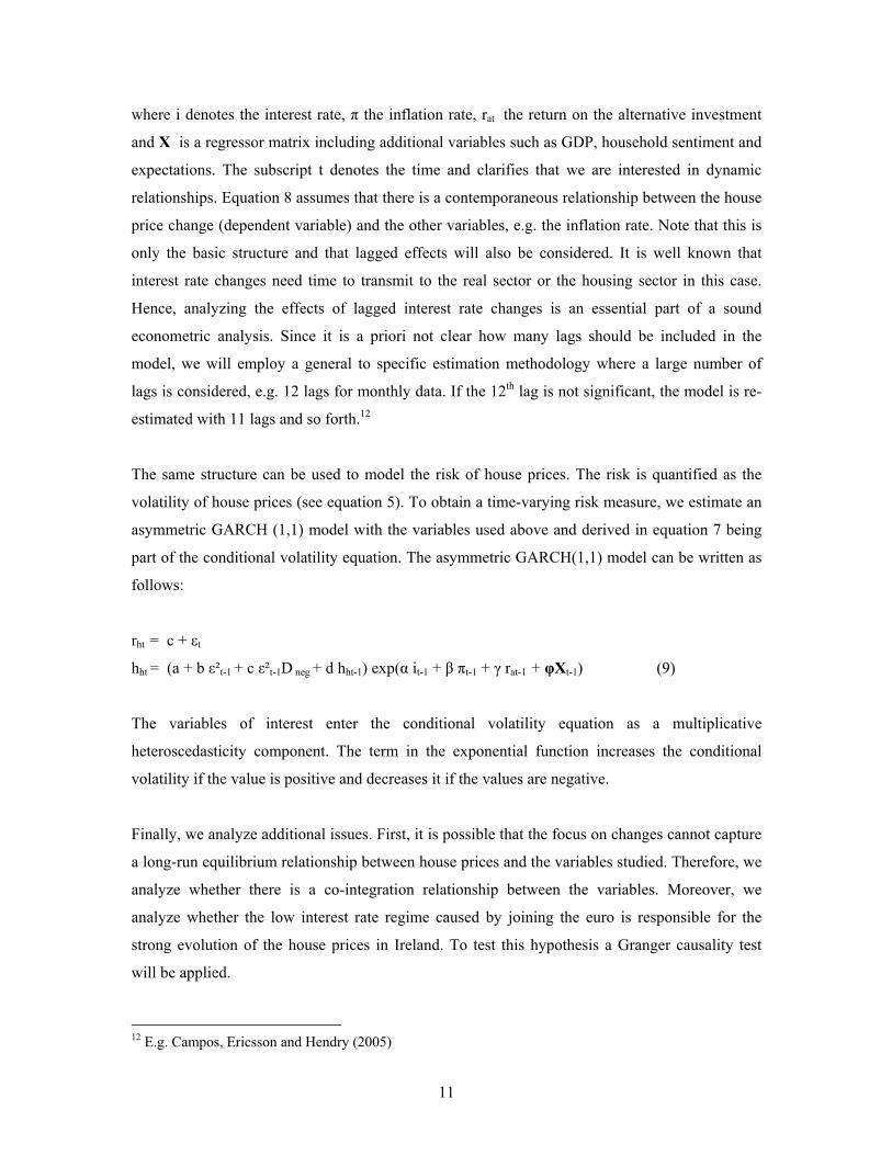
where i denotes the interest rate, π the inflation rate, rat the return on the alternative investment

and X is a regressor matrix including additional variables such as GDP, household sentiment and

expectations. The subscript t denotes the time and clarifies that we are interested in dynamic

relationships. Equation 8 assumes that there is a contemporaneous relationship between the house

price change (dependent variable) and the other variables, e.g. the inflation rate. Note that this is

only the basic structure and that lagged effects will also be considered. It is well known that

interest rate changes need time to transmit to the real sector or the housing sector in this case.

Hence, analyzing the effects of lagged interest rate changes is an essential part of a sound

econometric analysis. Since it is a priori not clear how many lags should be included in the

model, we will employ a general to specific estimation methodology where a large number of

lags is considered, e.g. 12 lags for monthly data. If the 12th lag is not significant, the model is re-

estimated with 11 lags and so forth.12

The same structure can be used to model the risk of house prices. The risk is quantified as the

volatility of house prices (see equation 5). To obtain a time-varying risk measure, we estimate an

asymmetric GARCH (1,1) model with the variables used above and derived in equation 7 being

part of the conditional volatility equation. The asymmetric GARCH(1,1) model can be written as

follows:

rht = c + εt

hht = (a + b ε²t-1 + c ε²t-1D neg + d hht-1) exp(α it-1 + β πt-1 + γ rat-1 + φXt-1) (9)

The variables of interest enter the conditional volatility equation as a multiplicative

heteroscedasticity component. The term in the exponential function increases the conditional

volatility if the value is positive and decreases it if the values are negative.

Finally, we analyze additional issues. First, it is possible that the focus on changes cannot capture

a long-run equilibrium relationship between house prices and the variables studied. Therefore, we

analyze whether there is a co-integration relationship between the variables. Moreover, we

analyze whether the low interest rate regime caused by joining the euro is responsible for the

strong evolution of the house prices in Ireland. To test this hypothesis a Granger causality test

will be applied.

12 E.g. Campos, Ericsson and Hendry (2005)

11

III. Empirical Analyses

This chapter first describes the data used for the study in section A and then presents the

estimation results in section B.

A. Descriptive Statistics

We use aggregate monthly data of Irish macroeconomic variables and survey data obtained from

Reuters Ecowin, Datastream and permanent tsb. The sample spans a time period of 12 years from

April 1996 to December 2007 yielding 141 observations per time series. Table 1 displays the

summary statistics for all variables in the data set starting with the nominal interest rate (3-month

rate), the stock market (ISEQ20), production and three different house price indices (first time

buyers, new houses and existing houses). The table also includes series based on survey data

complied by the European Commission (DGECFIN), unemployment and employment, earnings

and the consumer price index (CPI). The survey data is explained in more detail in table 1*.

Table 1 reports the mean, the standard deviation and the minimum and maximum values of the

log-changes of the variables.13 Some values are of particular interest in this study. For example,

the average interest rate change is negative for the sample period which can be attributed to the

adoption of the euro currency (see also figure 1). Moreover, while the stock market returns are

positive on average with a value of 0.0074 and a standard deviation of 0.0526, it is important to

note that the average returns of the house price indices are larger (between 0.0091 and 0.0097)

with a standard deviation around 0.01. This implies that housing investment exhibited higher

returns than stock markets at a lower risk. Finally, the average (monthly) inflation rate (cpi) is

0.0028 amounting to values around 3% per year.

Table 2 reports the unconditional correlations of the log-changes of five key macroeconomic

variables, that is, house prices (existing), the interest rate, the stock market, production, earnings

and cpi. The table shows the correlations for the full sample period and two sub-samples, a pre-

Euro sample and a post-Euro (introduction) sample. The main findings are that house prices are

negatively correlated with the other variables (except cpi) but with relatively low absolute

numbers. This pattern changes significantly for the post-Euro period for which the unconditional

correlation is positive for the interest rate, the stock market, earnings and cpi.

13 We use logarithmic changes because since in this case the coefficient estimates can be interpreted as elasticities.

12

These results show that there is a positive co-movement between house prices and interest rates,

the stock market, earnings and 12-month changes in cpi, which suggests that a house can serve as

a hedge against rising interest rates and inflation. However, despite the relatively low

correlations, it is important to stress that these results are based on unconditional correlations

which implies that they represent the isolated effect on house prices. The regression results below

will clarify that there are important differences if all variables are considered jointly and not

separately. Such a joint consideration is also consistent with the main question addressed in this

paper since a typical household is not exposed to just one economic risk but to several different

risks simultaneously.

< Insert table 1 about here >

< Insert table 2 about here >

< Insert figure 1 about here >

B. Estimation Results

This section presents the estimation results of the regression models outlined in the econometric

framework.

B1. House Price Determinants

Table 3 presents the estimation results of the regression model chosen with a general-to-specific

estimation technique. The dependent variable is the log change of the house price (existing house

price index) and the regressors are interest rates, inflation, stock market returns and production as

a proxy for the business cycle.14 The regression results show that the interest rate plays a

significant role in the determination of the house prices. Rising interest rates decrease house

prices and falling interest rates increase them. Note that there is a contemporaneous effect (-

0.0356) and lagged effects (3-month lag (0.0489) and 6-month lag (-0.0455)). The aggregate

effect is negative (-0.0322) and given by the sum of the contemporaneous effect and the lagged

effects. An alternative estimation without any lagged effects of the interest rate yields a

14 Production figures were used due to their availability on a monthly basis. GDP data is only available on a quarterly basis.

13

coefficient estimate of -0.02547. The coefficient estimate of the log-change in the consumer price

index (cpi) is negative and the effect of the returns of the stock market (ISEQ20) is positive.

However, both coefficient estimates are statistically insignificant. Finally, the effect of production

representing the business cycle appears to be the most important variable since the coefficient

estimates of the contemporaneous and lagged effects are all positive and significant. This implies

that there is a strong co-movement of house prices and the business cycle. Other variables such as

earnings or employment (see table 1 for details) were also considered but are not included in the

final model due to economically and/ or statistically insignificant coefficient estimates.

< Insert table 3 about here >

It is possible that the relationships changed with the introduction of the Euro currency. Thus, we

divide the full sample into two sub-samples. Table 4 shows the results for the period prior to the

Euro introduction in 1999 and table 5 shows the results for the period after the introduction of the

euro. Major differences for the pre-euro period are the contemporaneous negative effect of the

interest rate (no significant lagged effect), the positive and relatively large coefficient above 1.3

for inflation (cpi) though statistically insignificant and the negative relation of house prices with

the stock market (-0.1183). Finally, the coefficient estimates representing the influence of the

business cycle (production) are considerably larger in the pre-Euro era compared to the full

sample. The overall explanation of the variables, however, is similar (34% for the full period and

32% for the pre-Euro period). The results for the post-Euro period show that all variables have a

smaller absolute influence on house prices than in the pre-Euro period. The estimates are

insignificant for interest rates, inflation and the stock market and the business cycle effect is still

significant but the coefficients are clearly smaller. These results indicate that the influence and

thus exposure has changed over the years and is smaller in the post-Euro introduction era than in

the pre-Euro era. Before concluding that the Irish housing market has decoupled from the real

sector and was more driven by speculation or other factors, we further investigate the post-Euro

episode by estimating a rolling windows regression with a 36-month window length. The results

confirm the pre-Euro and post-Euro estimation results and additionally show that there is a strong

downward trend for inflation (cpi), an upward trend for the stock market and large swings around

zero for the interest rate and production. The coefficient estimates are larger than one for cpi in

the beginning of the sample and become negative in the end of the sample with values around -

0.3. The magnitude of the effects for the other variables is relatively small compared to the

estimates for cpi and range between -0.05 and +0.05.

14

It is thus appropriate to conclude that the Irish housing market has temporarily decoupled from

the business cycle and Euro zone interest rates. The negative impact of inflation on house prices

implies that inflation hurts Irish households through lower house prices and higher prices for

goods and services.

< Insert table 4 about here >

< Insert table 5 about here >

B2. House Price Volatility

This section presents estimation results that illustrate the relationship between macroeconomic

variables and the risk (volatility) of the average house price in Ireland. The estimation results are

based on equation 9 and are presented in table 6. In addition, figure 2 shows the relation of the

house price index and the estimated risk (volatility) of this index through time.

Table 6 shows that all key macroeconomic variables (interest rate, the stock market, production

and inflation (cpi)) influence the conditional volatility of the average house price. The interest

rate exhibits a negative relation with the house price index while the other variables display a

positive relation with the index. Thus, the interest rate tends to lower the conditional volatility

while the other variables tend to increase the risk of investments in the housing market. The

GARCH model estimates are significant (0.55 is the ARCH coefficient estimate and 0.53 is the

GARCH estimate) in contrast to the asymmetric component (threshold ARCH) which negative

and statistically insignificant. The relatively large coefficient estimate suggests, however, that

there is some economically significant effect implying that negative shocks increase the risk more

than positive shocks.

< Insert table 6 about here >

< Insert figure 2 about here >

B3. Calibration of Optimal Capital Allocation

This section presents the results of a calibration exercise with the objective to obtain time-varying

estimates of the average percentage amount invested in the housing sector. This figure is obtained

by using equation 6 (m* = [E(rh)-rf)]/ γ f(i, π, g, ra) ) and calibrating gamma by assuming an

15

average value (through time) for m*. The other variables are part of the data set and can thus be

used to compute a time-varying estimate for m* denoted as mt* conditional the average value for

m*. The main interest is thus not the level but the variation through time. Figures 3 and 4 present

the estimates for average values of m* equal to 1 and 0.5, respectively.

< Insert figure 3 about here >

< Insert figure 4 about here >

The figures show that there is a significant degree of variation ranging from -4 to +4 for m*=1 on

average and from -2 to +2 for m*=0.5. High values of m indicate a high degree of leverage. Not

surprisingly, periods with a relatively high m coincide with increasing house prices. A negative

value of m means an overinvestment of wealth in risk-free assets. The realizations of m can be

used as an indicator that shows changes in the average degree of borrowing or lending.

B4. Alternative Determinants

This section goes beyond the theoretical models’ variables and uses alternative variables in the

regressions. Two different models are considered. The first model re-estimates the basic

regression model but uses an alternative consumer price index comprising only alcoholic

beverages, tobacco and narcotics. The second model only considers consumer survey data (all

DGECFIN variables available) as potential regressors. The results are presented in table 7 and

show that the alternative consumer price index is positive and significant which contrasts the

findings for the commonly used CPI. Since the alternative index is only available for the last five

years of the sample, the results are based on a sub-sample of the post-Euro period. The fact that

production is not significant (contemporaneous and lags) is not counter to the findings obtained

before but only due to the restricted sample period. Note that only the last 5 years of the sample

are used in the estimation.

< Insert table 7 about here >

The second model uses all sixteen survey indicators in an initial regression and then applies the

general to specific methodology by subsequently eliminating all variables that are insignificant.

This procedure yields a specification with three variables, that is, a consumer survey based on the

economic conditions over the last 12 months, a survey on major purchases over the next 12

16

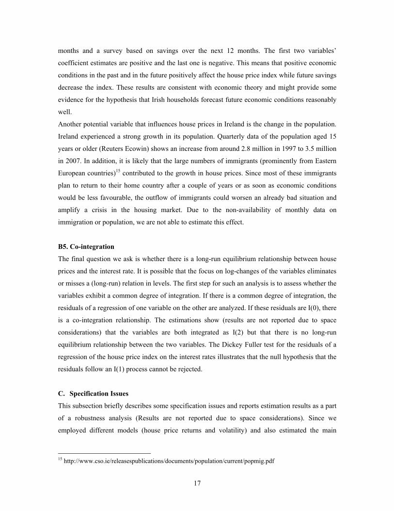
months and a survey based on savings over the next 12 months. The first two variables’

coefficient estimates are positive and the last one is negative. This means that positive economic

conditions in the past and in the future positively affect the house price index while future savings

decrease the index. These results are consistent with economic theory and might provide some

evidence for the hypothesis that Irish households forecast future economic conditions reasonably

well.

Another potential variable that influences house prices in Ireland is the change in the population.

Ireland experienced a strong growth in its population. Quarterly data of the population aged 15

years or older (Reuters Ecowin) shows an increase from around 2.8 million in 1997 to 3.5 million

in 2007. In addition, it is likely that the large numbers of immigrants (prominently from Eastern

European countries)15 contributed to the growth in house prices. Since most of these immigrants

plan to return to their home country after a couple of years or as soon as economic conditions

would be less favourable, the outflow of immigrants could worsen an already bad situation and

amplify a crisis in the housing market. Due to the non-availability of monthly data on

immigration or population, we are not able to estimate this effect.

B5. Co-integration

The final question we ask is whether there is a long-run equilibrium relationship between house

prices and the interest rate. It is possible that the focus on log-changes of the variables eliminates

or misses a (long-run) relation in levels. The first step for such an analysis is to assess whether the

variables exhibit a common degree of integration. If there is a common degree of integration, the

residuals of a regression of one variable on the other are analyzed. If these residuals are I(0), there

is a co-integration relationship. The estimations show (results are not reported due to space

considerations) that the variables are both integrated as I(2) but that there is no long-run

equilibrium relationship between the two variables. The Dickey Fuller test for the residuals of a

regression of the house price index on the interest rates illustrates that the null hypothesis that the

residuals follow an I(1) process cannot be rejected.

C. Specification Issues

This subsection briefly describes some specification issues and reports estimation results as a part

of a robustness analysis (Results are not reported due to space considerations). Since we

employed different models (house price returns and volatility) and also estimated the main

15 http://www.cso.ie/releasespublications/documents/population/current/popmig.pdf

17

models for the full sample and two (pre- and post-Euro) sub-samples including an analysis of the

last six years (table 7), the main estimation results already include basic robustness checks.

All results are based on a house price index for existing houses. If we re-estimate the model with

two alternative house price indices (new houses and first-time buyer houses), the results are

different. The major difference is in the coefficient estimates for inflation. While the coefficient is

negative for the ‘new house’-index, it is positive for the ‘first-time buyer’ house price index. The

goodness of fit (R squared) falls from 27% for the original model to 18% for the first-time buyers

and to 14% for the ‘new house’ index.

The model for the volatility of house prices (GARCH model) was also re-estimated for the two

sub-samples and the results are consistent with the findings for the main model. Finally, including

the variables also in the mean equation does not qualitatively change the results in the variance

equation.

IV. Conclusions

This study analyzed the relation of house prices with key economic variables in order to assess

the exposure of a typical Irish household to economic risks such as interest rate changes, inflation

and the business cycle. The empirical analysis of a newly compiled data set, comprising monthly

data over the last 12 years shows that investments in the Irish housing market have yielded high

returns with a relatively low level of risk compared to the Irish stock market index. The

regression results further show that house owners are negatively exposed to positive interest rate

changes, higher inflation and lower or negative growth rates of the economy. The exposure is not

problematic in times of low interest rates, moderate inflation and high economic growth but poses

severe risks to households if inflation increases, interest rates go up and economic growth slows.

We further argue that the introduction of the Euro added to the total risk since interest rates and

the business cycle can move simultaneously in unfavourable directions rendering the joint

exposure larger. If Ireland is in a low-growth regime and the major EU countries are in a high-

growth regime with increasing interest rates, Irish households might be affected by falling house

prices, higher mortgage payments and the risk of becoming unemployed.

This paper aims to raise awareness that house buyers need to consider all relevant risks involved

in the purchase of a house. It has been rational for a long time for Irish households to hold the

majority of their assets in their houses, but this is unlikely to be the case going forward, as

18

macroeconomic risk factors to which households are exposed now begin to move in unfavourable

directions.

The economic framework emphasizing the choices of rational households and the empirical

results show that the purchase of a house is risky and should not be considered as a natural form

of investment

19

References

Ahearne, A., J. Ammer, B. Doyle, L. Kole & R. Martin (2005), “House Prices and Monetary Policy: A Cross-Country Study”, International Finance Discussion Paper 841, Board of Governors of the Federal Reserve System, September Aksoy, Y., P. de Grauwe & H. Dewachter (2002), “Do asymmetries matter for European monetary policy?”, European Economic Review 46 Anari, A. & J. Kolari (2002), “House Prices and Inflation”, Real Estate Economics, Vol 30 No. 1 Bond, M. & M. Seiler (1998), “Real Estate Returns and Inflation: An Added Variable Approach”, Journal of Real Estate Research, Vol 15 No. 3 Borio, C. & P. McGuire (2004), “Twin Peaks in Equity and Housing Prices?”, BIS Quarterly Review, March Case, K. & R. Schiller (2003), “Is there a bubble in the Housing Market?”, Brookings Papers on Economic Activity, Vol 2003 No. 2 Campos, J., Ericsson, N. R. and D.F. Hendry, (2005), "General-to-Specific Modeling: An Overview and Selected Bibliography", FRB International Finance Discussion Paper No. 838 Available at SSRN: http://ssrn.com/abstract=791684 Central Bank and Financial Services Authority of Ireland (2006), “Financial Stability Report”, in Annual Report 2006 Central Bank and Financial Services Authority of Ireland (2007), “Sectoral Developments in Private-Sector Credit”, December Fitzpatrick, T. & K. McQuinn (2007), “House prices and mortgage credit: empirical evidence for Ireland”, The Manchester School, Vol 75 No. 1 Hoesli, M., B. Macgregor, G. Matysiak & N. Nanthakumaran (1997), “The Short-term Inflation-hedging Characteristics of U.K. Real Estate”, Journal of Real Estate, Finance and Economics, Vol 15 No. 1 Huang, H. & S. Hudson-Wilson (2007), “Private Commercial Real Estate Equity Returns and Inflation”, Journal of Portfolio Management, Special Real Estate Issue Iacoviello, M. & R. Minetti (2003), “Financial Liberalization and the Sensitivity of House Prices to Monetary Policy: Theory and Evidence”, The Manchester School, Vol 71 No. 1 IMF (2008), “The changing housing cycle and the implications for monetary policy”, World Economic Outlook, April Kelly, J. & A. Menton (2007), “Residential Mortgages: Borrowing for Investment”, Central Bank and Financial Services Authority of Ireland, Quarterly Bulletin 2

20

21

Maclennan, D., J. Muellbauer & M. Stephens (1998), “Asymmetries in housing and financial market institutions and EMU”, Oxford Review of Economic Policy, Vol 14 No. 3. Updated July 2000 McQuinn, K. & G. O’Reilly (2006), “Assessing the Role of Income and Interest Rates in Determining Irish House Prices”, Central Bank and Financial Services Authority of Ireland, Financial Stability Report McQuinn, K. & G. O’Reilly (2007), “A Model of Cross-Country House Prices”, Research Technical Paper, Central Bank and Financial Services Authority of Ireland, July McQuinn, K. (2004), “A Model of the Irish Housing Sector”, Research Technical Paper, Central Bank and Financial Services Authority of Ireland, April National Irish Bank (2008), “The Emerald Isle: The Wealth of Modern Ireland”, February OECD (2006a), “Recent House Price Developments: The Role of Fundamentals”, OECD Economic Outlook No. 78 OECD (2006b), “Has the Rise in Debt made Households more Vulnerable?”, OECD Economic Outlook No. 80 Rae, D. & P. van den Noord (2006), “Ireland’s housing boom: what has driven it and have priced overshot?”, OECD, Working Paper, June Roche, M. (2001), “The rise in house prices in Dublin: bubble, fad or just fundamentals”, Economic Modelling, Vol 18 Issue 2 Stevenson, S. (2008), “Modelling Housing Market Fundamentals: Empirical Evidence of Extreme Market Conditions”, Real Estate Economics, Vol 36 No. 1

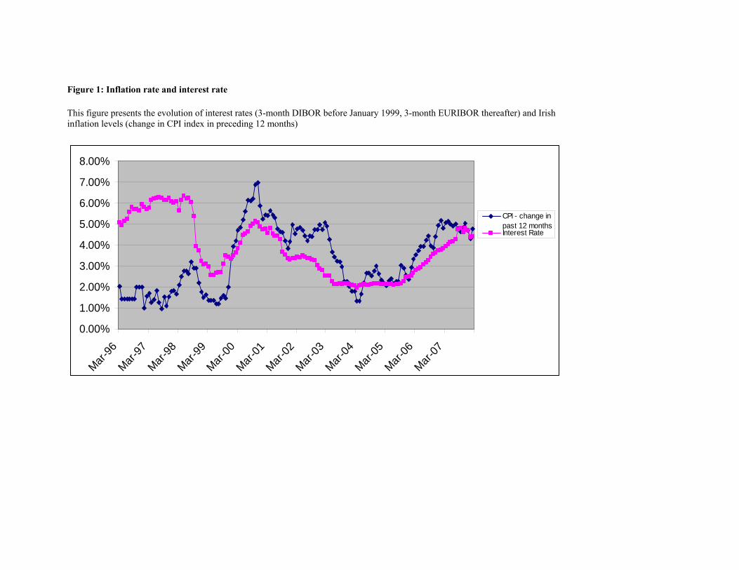
Figure 1: Inflation rate and interest rate This figure presents the evolution of interest rates (3-month DIBOR before January 1999, 3-month EURIBOR thereafter) and Irish inflation levels (change in CPI index in preceding 12 months)

0.00%

1.00%

2.00%

3.00%

4.00%

5.00%

6.00%

7.00%

8.00%

Mar-96

Mar-97

Mar-98

Mar-99

Mar-00

Mar-01

Mar-02

Mar-03

Mar-04

Mar-05

Mar-06

Mar-07

CPI - change inpast 12 monthsInterest Rate

Figure 2: Variance (GARCH estimates) of house prices The figure presents the evolution of the house price index and the estimated conditional volatility of that index.

0

20

40

60

80

100

120

140

1996

:04:00

1996

:09:00

1997

:02:00

1997

:07:00

1997

:12:00

1998

:05:00

1998

:10:00

1999

:03:00

1999

:08:00

2000

:01:00

2000

:06:00

2000

:11:00

2001

:04:00

2001

:09:00

2002

:02:00

2002

:07:00

2002

:12:00

2003

:05:00

2003

:10:00

2004

:03:00

2004

:08:00

2005

:01:00

2005

:06:00

2005

:11:00

2006

:04:00

2006

:09:00

2007

:02:00

2007

:07:00

2007

:12:00

0

0.0002

0.0004

0.0006

0.0008

0.001

0.0012

House Pricesvar_garch

23

Figure 3: Optimal investment in real estate (m*) The figure shows the time-variation of m calibrated to be one (m=1) on average based on m* = [E(rh)-rf)]/ γ f(i, π, g, ra) with monthly data.

-5

-4

-3

-2

-1

0

1

2

3

4

5

6

1996

:04:00

1996

:08:00

1996

:12:00

1997

:04:00

1997

:08:00

1997

:12:00

1998

:04:00

1998

:08:00

1998

:12:00

1999

:04:00

1999

:08:00

1999

:12:00

2000

:04:00

2000

:08:00

2000

:12:00

2001

:04:00

2001

:08:00

2001

:12:00

2002

:04:00

2002

:08:00

2002

:12:00

2003

:04:00

2003

:08:00

2003

:12:00

2004

:04:00

2004

:08:00

2004

:12:00

2005

:04:00

2005

:08:00

2005

:12:00

2006

:04:00

2006

:08:00

2006

:12:00

2007

:04:00

2007

:08:00

2007

:12:00

24

Figure 4: Optimal investment in real estate (m*) The figure shows the time-variation of m calibrated to be 0.5(m=0.5) on average based on m* = [E(rh)-rf)]/ γ f(i, π, g, ra) with monthly data:

0

20

40

60

80

100

120

140

160

1996

:04:00

1996

:09:00

1997

:02:00

1997

:07:00

1997

:12:00

1998

:05:00

1998

:10:00

1999

:03:00

1999

:08:00

2000

:01:00

2000

:06:00

2000

:11:00

2001

:04:00

2001

:09:00

2002

:02:00

2002

:07:00

2002

:12:00

2003

:05:00

2003

:10:00

2004

:03:00

2004

:08:00

2005

:01:00

2005

:06:00

2005

:11:00

2006

:04:00

2006

:09:00

2007

:02:00

2007

:07:00

2007

:12:00

-2.5

-2

-1.5

-1

-0.5

0

0.5

1

1.5

2

2.5

3

House Pricesm* (contemporaneous)

25

Table 1: Descriptive Statistics The table displays the descriptive statistics of all variables in the sample. The columns contain the number of observations, the mean, the standard deviation, the minimum and the maximum value of the variable. Variable (log-changes) Obs Mean Std. Dev. Min Max

Interest rate 141 -0.0006 0.0519 -0.3112 0.1347

Stock market 141 0.0074 0.0526 -0.1710 0.1417

Production 141 0.0068 0.0885 -0.2674 0.2033

house price first 141 0.0097 0.0105 -0.0180 0.0441

House price new 141 0.0091 0.0098 -0.0151 0.0377

House price exist 141 0.0096 0.0107 -0.0231 0.0477

dgecfin1 141 -0.0014 0.0394 -0.1034 0.0866

dgecfin2 141 1.2610 10.4226 -22.1000 18.9000

Consumer Survey1 141 -0.0035 0.0514 -0.1405 0.1194

Consumer Survey2 141 -0.0019 0.0442 -0.0938 0.1666

Consumer Survey3 141 -0.0049 0.0765 -0.2367 0.2228

cars 141 -0.0166 0.6220 -0.7847 2.9655

Unemployment (male) 141 -0.0037 0.0256 -0.0613 0.0556

Unemployment (female) 141 -0.0033 0.0547 -0.1769 0.1280

Unemployment total 141 -0.0036 0.0357 -0.1076 0.0772

Employment total 141 0.0019 0.0314 -0.0754 0.0923

Earnings 135 0.0043 0.0061 -0.0086 0.0165

cpi 141 0.0028 0.0040 -0.0086 0.0118

26

Table 1*: Indicators Indicator Description

DG ECFIN1 Economic Sentiment Economic sentiment indicator

DG ECFIN2 Consumer Surveys Confidence indicator

Consumer Surveys1 Consumer Sentiment Index (IIB Bank/ESRI)

Consumer Surveys2 Current Economic Conditions Index (IIB Bank/ESRI)

Consumer Surveys3 Consumers Expectations Index (IIB Bank/ESRI)

DG ECFIN6 Consumer Surveys Financial situation of households over last 12 months

DG ECFIN7 Consumer Surveys Financial situation of households over next 12 months

DG ECFIN8 Consumer Surveys General economic situation over last 12 months

DG ECFIN9 Consumer Surveys General economic situation over next 12 months

DG ECFIN10 Consumer Surveys Major purchases at present

DG ECFIN11 Consumer Surveys Major purchases over next 12 months

DG ECFIN12 Consumer Surveys Unemployment expectations over next 12 months

DG ECFIN13 Consumer Surveys Price trends over last 12 months

DG ECFIN14 Consumer Surveys Price trends over next 12 months

DG ECFIN15 Consumer Surveys Savings at present 12 months

DG ECFIN16 Consumer Surveys Savings over next 12 months

27

Table 2: Unconditional correlations (full sample, pre-Euro and post-Euro) The table shows the unconditional correlations between key macroeconomic variables: a house price index (existing houses), interest rate, the stock market, production, earnings and cpi. Full sample (N=135) House prices Interest

rate Stock market

Production earnings

House prices 1

Interest rate -0.0573 1

Stock market -0.0514 0.0345 1

Production -0.0085 0.03510.0153 1

Earnings -0.0752 -0.0141-0.0498 -0.0608 1

Cpi 0.0121 0.0918 -0.0578 0.2804 0.0329

Pre Euro sample (N=35) House prices Interest rate

Stock market

Production earnings

House prices 1

Interest rate -0.1542 1

Stock market -0.303 -0.0785 1

Production 0.0791 0.0633-0.2675 1

Earnings -0.3863 0.0418-0.0593 -0.069 1

Cpi 0.1151 -0.12810.1231 0.0341 0.099

Post Euro sample (N=100) House prices Interest rate

Stock market

Production earnings

House prices 1

Interest rate 0.0876 1

Stock market 0.0102 0.1389 1

Production -0.0557 0.02260.1451 1

Earnings 0.1361 -0.0176-0.0663 -0.0566 1

cpi 0.0528 0.00670.0404 0.3539 -0.0116

28

Table 3: Regression results The table presents the estimation results of a regression of the house price changes on interest rates, inflation, stock market returns and the business cycle. In order to determine the number of lags a general-to-specific estimation methodology is chosen. Coef. Std. Err t-stat.

interest -0.0356 0.0171 -2.08 **

L3. 0.0489 0.0186 2.63 ***

L6. -0.0455 0.0172 -2.65 ***

cpi -0.0955 0.2528 -0.38

stockm 0.0050 0.0162 0.31

prod 0.0231 0.0125 1.85 *

L1. 0.0359 0.0132 2.72 ***

L2. 0.0530 0.0150 3.52 ***

L3. 0.0480 0.0156 3.07 ***

L4. 0.0856 0.0162 5.3 ***

L5. 0.0935 0.0165 5.67 ***

L6. 0.0958 0.0166 5.79 ***

L7. 0.0613 0.0154 3.98 ***

L8. 0.0569 0.0145 3.92 ***

L9. 0.0393 0.0133 2.96 **

L10. 0.0244 0.0119 2.05 **

const. 0.0052 0.0013 3.9 ***

F (16,114) 3.60 ***

R squared 0.3358

29

Table 4: Regression results (pre-Euro) The table presents the estimation results of a regression of the house price changes on interest rates, inflation, stock market returns and the business cycle for the period prior to the Euro introduction (pre-Euro). In order to determine the number of lags a general-to-specific estimation methodology is chosen. Coef. Std. Err. t-stat

interest -0.0799 0.0407 -1.96 **

cpi 1.2684 1.1227 1.13

stock market -0.1183 0.0535 -2.21 *

prod 0.0191 0.0490 0.39

L1. 0.0642 0.0662 0.97

L2. 0.1125 0.0674 1.67

L3. 0.1550 0.0896 1.73

L4. 0.2468 0.0825 2.99 **

L5. 0.2262 0.0872 2.59 **

L6. 0.2045 0.0790 2.59 **

L7. 0.1399 0.0626 2.23 **

L8. 0.1435 0.0538 2.67 **

L9. 0.0775 0.0416 1.86 *

const. -0.0057 0.0088 -0.66

Number of obs. 25

F(14,10) 1.81

R squared 0.3197

30

Table 5: Regression results (post-Euro) The table presents the estimation results of a regression of the house price changes on interest rates, inflation, stock market returns and the business cycle for the period after the Euro introduction (post-Euro). In order to determine the number of lags a general-to-specific estimation methodology is chosen. Coef. Std. Err. t-stat

Interest -0.0066 0.0211 -0.31

Cpi -0.0511 0.2710 -0.19

Stock market 0.0217 0.0183 1.19

Production 0.0130 0.0135 0.96

L1. 0.0333 0.0142 2.35 **

L2. 0.0443 0.0162 2.74 ***

L3. 0.0458 0.0169 2.7 ***

L4. 0.0637 0.0180 3.53 ***

L5. 0.0731 0.0185 3.95 ***

L6. 0.0731 0.0186 3.93 ***

L7. 0.0487 0.0166 2.94 ***

L8. 0.0422 0.0157 2.68 ***

L9. 0.0331 0.0141 2.35 **

L10. 0.0212 0.0127 1.67 *

const. 0.0052 0.0013 3.86 ***

Number of obs. 106

F(14,91) 1.65 *

R squared 0.2024

31

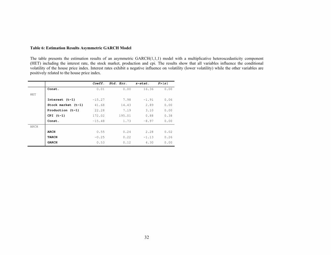
Table 6: Estimation Results Asymmetric GARCH Model The table presents the estimation results of an asymmetric GARCH(1,1,1) model with a multiplicative heteroscedasticity component (HET) including the interest rate, the stock market, production and cpi. The results show that all variables influence the conditional volatility of the house price index. Interest rates exhibit a negative influence on volatility (lower volatility) while the other variables are positively related to the house price index. Coeff. Std. Err. z-stat. P>|z|

Const. 0.01 0.00 16.36 0.00

HET

Interest (t-1) -15.27 7.98 -1.91 0.06

Stock market (t-1) 41.68 14.43 2.89 0.00

Production (t-1) 22.28 7.19 3.10 0.00

CPI (t-1) 172.02 195.01 0.88 0.38

Const. -15.48 1.73 -8.97 0.00

ARCH

ARCH 0.55 0.24 2.28 0.02

TARCH -0.25 0.22 -1.13 0.26

GARCH 0.53 0.12 4.30 0.00

32

Table 7: Alternative determinants The table presents estimation results for two models with alternative variables. Model 1 shows the regression results for an alternative consumer price index only comprising alcoholic beverages, tobacco and narcotics. Model 2 shows the regression results for consumer survey indicators. The three indicators reported are selected with a general-to-specific estimation strategy starting with 16 indices (see descriptive statistics). Model 1 Coef. Std. Err. t-stat

Interest rate -0.0656 0.0293 -2.24 **

cpi (alcoholic beverages, drugs etc.)

0.3813 0.1895 2.01 **

Stock market return 0.0398 0.0207 1.92 *

Production change 0.0036 0.0112 0.32

const. 0.0052 0.0012 4.40 ***

F(4,67) 3.06 **

R squared 0.1545

Model 2 Coef. Std. Err. t-stat

Consumer survey (economic condition over last 12 months)

0.0579 0.0346 1.68 *

Consumer survey (major purchases next over 12 months)

1.0387 0.2405 4.32 ***

Consumer survey (savings over next 12 months)

-0.4790 0.1165 -4.11 ***

const. 22.2353 2.6675 8.34 ***

F(3,137) 15.56 ***

R squared 0.2542

33

Institute for International Integration StudiesThe Sutherland Centre, Trinity College Dublin, Dublin 2, Ireland