
DUALITY THEORY FOR COMPOSITE GEOMETRIC...
166
DUALITY THEORY FOR COMPOSITE GEOMETRIC PROGRAMMING by Ya-Ping Wang B.S. Mathematics, National Tsing-Hua University, 1973 M.A. Mathematical Statistics, Wayne State University, 1979 M.S. Applied Mathematics, Carnegie Mellon University, 1982 Submitted to the Graduate Faculty of Swanson School of Engineering in partial fulfillment of the requirements for the degree of Doctor of Philosophy University of Pittsburgh 2013
Transcript of DUALITY THEORY FOR COMPOSITE GEOMETRIC...

By
[Ya-Ping Wang],
[M.A./M.S./PhD]
Submitted to the Graduate Faculty of
School of Engineering in partial fulfillment
of the requirements for the degree of
Doctor of Philosophy
University of Pittsburgh
2012
DUALITY THEORY FOR COMPOSITE GEOMETRIC PROGRAMMING
by
Ya-Ping Wang
B.S. Mathematics, National Tsing-Hua University, 1973
M.A. Mathematical Statistics, Wayne State University, 1979
M.S. Applied Mathematics, Carnegie Mellon University, 1982
Submitted to the Graduate Faculty of
Swanson School of Engineering in partial fulfillment
of the requirements for the degree of
Doctor of Philosophy
University of Pittsburgh
2013

ii
UNIVERSITY OF PITTSBURGH
SWANSON SCHOOL OF ENGINEERING
This dissertation was presented
by
Ya-Ping Wang
It was defended on
December 14, 2012
and approved by
Oleg A. Prokopyev, PhD, Associate Professor, Department of Industrial Engineering
Denis R. Saure, PhD, Assistant Professor, Department of Industrial Engineering
Zhi-Hong Mao, PhD, Associate Professor, Department of Electrical and Computer Engineering
Dissertation Director: Jayant Rajgopal, PhD, Associate Professor, Department of Industrial
Engineering

iii
Copyright © by Ya-Ping Wang
2013

iv
This research develops an alternative approach to the duality theory of the well-known
subject of Geometric Programming (GP), and uses this to then develop a duality theory for
Quadratic Geometric Programming (QGP), which is an extension of GP; it then develops a
duality theory for (convex) Composite Geometric Programming (CGP), which in turn, is a
generalization of QGP. The building block of GP is a special class of functions called
posynomials, which are summations of terms, where the logarithm of each term is a linear
function of the logarithms of its design variables. Such log-linear relationships often appear as
an empirical fit in numerous engineering applications, most notably in engineering design. At
other times, these relationships may simply follow the dictates of the laws of nature and/or
economics (Varian 1978). Many functions that describe engineering systems are posynomials
and hence GP is especially suitable for handling optimization problems involving such functions.
For instance, the so-called Machining Economics Problem (MEP) for conventional metals can be
handled successfully by GP (Tsai, 1986). The defining relationship of the tool life as a function
of machining variables such as cutting speed, depth of cut, feed rate, tool change downtime, etc.,
is typically log-linear.
However, when the logarithm of the tool life for a given alloy is a quadratic (instead of a
linear) function of the logarithms of the machining variables, GP is not able to handle this kind
of MEP (Hough, 1978; Hough and Goforth, 1981a, b, c). Jefferson and Scott (1985) introduced
DUALITY THEORY FOR COMPOSITE GEOMETRIC PROGRAMMING
Ya-Ping Wang, PhD
University of Pittsburgh, 2013

v
QGP to successfully handle the quadratic version of the MEP. They also gave primal-dual
formulations of the QGP problem, an optimality condition, and three illustrative numerical
examples of MEP (Jefferson and Scott 1985, p.144). A strong duality theorem for QGP was
later proved by Fang and Rajasekera (1987) using a dual perturbation approach and two simple
geometric inequalities.
However, more detailed duality theory for QGP and for CGP comparable to the
development for GP by Duffin, Peterson, and Zener in chapters IV and VI of their seminal text
(1967) are yet to be developed. This theory is rooted in the duality principle for ‘conjugate’ pairs
of convex functions, which translates the analysis of one optimization problem into an
equivalent, yet very different optimization problem. It allows us to view the problem from two
different angles, often with new insights and with other remarkable consequences such as
suggesting an easier solution approach. In this thesis, we extend QGP problems to the more
general CGP problems to account for the even more general log-convex (as opposed to log-
linear) relationships. The aim of this dissertation is to develop a comprehensive duality theory
for both QGP and CGP.

vi
TABLE OF CONTENTS
ACKNOWLEDGMENTS ...................................................................................................... IX
1.0 INTRODUCTION .........................................................................................................1
1.1 OPTIMIZATION PROBLEMS .......................................................................2
1.2 GP AS A SUBCLASS OF CONVEX PROGRAMS ........................................7
1.3 EXTENSIONS TO EGP, QGP, AND THEN TO CGP .................................. 15
1.4 THESIS PLAN ................................................................................................ 22
2.0 LITERATURE REVIEW ON DUALITY THEORY ................................................ 23
2.1 DUAL PROGRAM GD AND DUALITY THEORY OF GP ........................ 23
2.2 ASSESSING A DUAL APPROACH TO GP ................................................. 32
2.3 FENCHEL’S DUALITY THEORY AND GENERALIZED GEOMETRIC
INEQUALITY ................................................................................................ 35
2.4 KKT THEOREM FOR CONVEX PROGRAMS .......................................... 50
2.5 THE EXISTENCE OF A PRIMAL MINIMAL SOLUTION........................ 53
3.0 ALTERNATIVE PROOFS AND SOME REFINEMENTS OF THE DUALITY
THEOREMS OF GP ................................................................................................... 60
3.1 MAIN LEMMA OF GP .................................................................................. 62
3.2 FIRST DUALITY THEOREM OF GP.......................................................... 66
3.3 SECOND DUALITY THEOREM OF GP ..................................................... 68

vii
4.0 DUALITY THEORY OF EXPONENTIAL GP ......................................................... 74
4.1 PROBLEM FORMULATION OF EGP ........................................................ 74
4.2 COMPOSITE GEOMETRIC FUNCTION ................................................... 79
4.3 DUAL PROGRAM EGD ................................................................................ 82
4.4 MAIN LEMMA OF EGP ............................................................................... 86
4.5 FIRST AND SECOND DUALITY THEOREMS OF EGP........................... 90
5.0 DUALITY THEORY OF COMPOSITE GP ............................................................. 95
5.1 PROBLEM FORMULATIONS OF CGP AND CGD ................................... 95
5.2 MAIN LEMMA OF CGP ............................................................................. 101
5.3 FIRST AND SECOND DUALITY THEOREMS OF CGP ........................ 103
6.0 DUALITY THEORY OF QUADRATIC GP ........................................................... 106
6.1 PROBLEM FORMULATIONS OF QGP ................................................... 106
6.2 MAIN LEMMA OF QGP ............................................................................. 111
6.3 FIRST AND SECOND DUALITY THEOREMS OF QGP ........................ 115
7.0 DUALITY THEORY OF LPGP AND QGP ............................................................. 122
7.1 PROBLEM FORMULATIONS OF LPGP AND LPGD............................... 122
7.2 MAIN LEMMA OF LPGP ............................................................................ 126
7.3 FIRST AND SECOND DUALITY THEOREMS OF LPGP ....................... 127
8.0 CONCLUSION AND SOME DIRECTIONS OF FUTURE RESEARCH.............. 130
8.1 SUMMARY OF CONTRIBUTIONS ........................................................... 130
8.2 SOME DIRECTIONS FOR FUTURE RESEARCH .................................. 131
APPENDIX A. MATHEMATICAL PROOF OF SOME INEQUALITIES ....................... 133
A.1 ON STRICTLY CONVEX FUNCTIONS .................................................... 133
viii
A.2 THE AGM INEQUALITY AND THE GEOMETRIC INEQUALITY...... 137
APPENDIX B. THE STIMULANT OF THE BIRTH OF GP– ZENER’S DISCOVERY . 141
APPENDIX C. EXTENDED REAL-VALUED FUNCTIONS AND SEQUENCES .......... 145
BIBLIOGRAPHY ................................................................................................................. 151

ix
ACKNOWLEDGMENTS
In memory of my parents: Yue-Tao Wang and Yu-Guei Tian.
The fear of the LORD is the beginning of wisdom: and the knowledge of the holy is
understanding. (Proverbs 9:10)
This dissertation was done in two stages with a very painful prolonged interruption of
more than a decade in between. In the proposal stage, it was under the guidance of Dr. T.R.
Jefferson with the title: Composite Geometric Programming-Theory and Application; and later in
the actual writing stage it is under the guidance of Dr. J. Rajgopal with the current title: Duality
Theory for Composite Geometric Programming.
The author hereby expresses his sincere gratitude towards the above two advisors for
their patient advice and guidance over all these years. It was Dr. T.R. Jefferson who introduced
me to the field of Peterson’s Generalized Geometric Programming, and this dissertation was
actually inspired from a paper he coauthored with Dr. C.H. Scott on Quadratic Geometric
Programming.
Then, after a number of years, the author communicated with Dr. J. Rajgopal, who took
over as my new advisor and agreed to let me resume writing this dissertation under the current

x
title. The author gratefully appreciates his kindness and the department’s approval for giving
him this second chance.
The author appreciates the Department of Industrial Engineering of this school for the 4
year teaching assistantships he received during his first stage of Ph.D study and for occasional
tuition waievers during his second stage. He also appreciates the emergency loans during his
financial crisis at the later stage from the following friends: Dr. Jen-Luen Chu, Dr. Zengbiao Qi,
Dr. Li Zou, and Dr. Ning Zhang, and relatives: Dr. Yue Chen and Dr. Wei Tian, without which
this dissertation could not possibly be completed.
Lastly, I would like to express my thankfulness to the late Professor R.J. Duffin for
getting me interested in the prototype posynomial programming from taking an introductory
course he offered on this subject at Carnegie-Mellon University. Most of the ideas I used while
developing this duality theory were obtained from the writings of Dr. J.M. Borwein, Dr. E.L.
Peterson, and Dr. R.T. Rockafellar. The author expresses his sincere thankfulness for their
pioneering work.

1
1.0 INTRODUCTION
This dissertation develops a comprehensive duality theory for (convex) Composite
Geometric Programming (CGP) as well as Quadratic Geometric Programming (QGP). QGP is
an extension of the well-known subject of Geometric Programming (GP), while CGP is in turn, a
generalization of QGP. QGP was first introduced [Jefferson and Scott, 1985] as a means to solve
a Machining Economics Problem (MEP) where the logarithm of the tool life for a given alloy is
modeled as a quadratic function of the logarithms of machining variables such as cutting speed,
depth of cut, feed rate, tool change downtime, etc. The MEP for conventional metals can be
handled successfully by GP (Tsai, 1986), since the defining relationship is log-linear. But with
alloys, the relationship becomes log-quadratic, and GP is not able to handle this case [Hough,
1978; Hough and Goforth, 1981a,b,c]. One has to then resort to QGP [Hough and Chang, 1998].
Jefferson and Scott [1985, p.144] gave the primal-dual formulations of the QGP problem, an
optimality condition, and three illustrative numerical examples of MEP. The main duality
theorem for QGP was later proved by Fang and Rajasekera [1987] using a dual perturbation
approach and two geometric inequalities. Jefferson et al. [1990] extend QGP problems to the
more general CGP problems to account for the more general log-convex relationships, where
primal-dual formulations of the CGP problems are provided, along with an optimality condition
(Theorems 4.1 and 5.1, pp.109-113), and two prior examples [Lidor and Wilde, 1978; Beightler

2
and Phillips, 1976] to illustrate the idea of the dual solution approach. However, more detailed
duality theory for QGP and for CGP comparable to the development for traditional GP by
Duffin, Peterson, and Zener in chapters IV and VI of their seminal text [1967] has never been
developed. This theory is rooted in the duality principle for ‘conjugate’ pairs of convex
functions, which translates the analysis of one optimization problem into an equivalent, yet very
different optimization problem. It allows us to view the problem from two different angles, often
with new insights and with other remarkable consequences such as suggesting an easier solution
approach. The aim of this dissertation is to develop a comprehensive duality theory for CGP,
and for several special cases of CGP including Exponential GP (EGP), QGP and lpGP.
Additional application of CGP can be found in Scott et al. [1996]. In a straightforward
manner, CGP formulations can also be further generalized to Composite Convex Programming
(CCP) problems [Scott and Jefferson, 1991]. Equation Chapter 1 Section 1
1.1 OPTIMIZATION PROBLEMS
Optimization problems are concerned with finding the maximum or minimum of a
function subject to some set of constraints. In this dissertation, we shall adopt minimization as
the main vehicle of exposition, leaving the parallel statements for maximization as unstated
results, since maximizing a function is simply equivalent to minimizing its negative. We shall
work in the real space Rn of column n-vectors equipped with the standard inner product. By an
Optimization Problem (OP) in Rn we shall mean mathematically:

3
(1.1)
0
1
2
( )
( ) 0 (OP) ( ) 0
i
i
inf f
s.t. f , i If , i I
C
≤ ∈
= ∈ ∈
xx
xxx
where x=(x1,…,xn)t ∈Rn represents a design or decision vector, nC R⊂ is a nonempty set of
“meaningful” values for the design vector, which often takes the form of a product set
1 nC C C= × ×L , where each Cj is a closed interval in R with nonempty interior. I1 and I2 are two
disjoint finite index sets with 1 2 I I I∪ = . Each problem-defining function
: , {0}if C R i I→ ∈ ∪ is real-valued, and the inequalities 1( ) 0if , i I≤ ∈x and the equations
2( ) 0,if i I= ∈x representing design specifications or restrictions (physical, technical, financial,
etc.) are called constraints. The classification of constraints into inequality ones and equality
ones is only a matter of formality. Mathematically speaking, there is no loss of generality in
assuming that all of the constraints (if any) are of inequality type, i.e. I2=φ, as
( ) 0 ( ) 0, and - ( ) 0.i i if f f= ⇔ ≤ ≤x x x There is also clearly no loss of generality in assuming
that the objective function f0, is linear; this can be done by mnimizing a new varaible x0 and
adding the new constraint f0(x) ≤ x0 .
Problem (OP) (1.1) is concerned with seeking the infimum of the objective function 0f
over its feasible region { }1 i 2( ) 0, ; ( ) 0,iS : C f i I f i I ,= ∈ ≤ ∈ = ∈x x x 0 0inf : inf{ ( ) | }S f f x S= ∈x ,
and its set of minimizers, { }0 0 0argmin := ( ) infS Sf S f f∈ =x x , when 0infS f < ∞ . It is said to be
feasible, if S is non-empty and infeasible, if otherwise. When (OP) is feasible (S≠φ) and 0infS f =
-∞, we say that (OP) has an unbounded infimum. By convention, we define 0infS f = +∞, if (OP)

4
is infeasible (S=φ). The major issues being considered in this problem (OP) are usually arranged
into three phases: feasibility, optimality, and sensitivity [Eiselt and Sandblom, 2007, p.57]. Note
that when I1=φ, C=Rn, and all of the problem-defining functions fi, {0}i I∈ ∪ are differentiable,
(1.1) is simply a classical optimization problem, which is typically solved by the method of
Lagrange multipliers [Luenberger, 1984, p.300]. It is termed a Linear Program (LP) or a Linear
Optimization Problem, if all of the problem-defining functions fi are affine (i.e. linear plus
constant) and each Ci=[0,∞), or =(-∞,∞) :=R; and an Ordinary Convex Program (OCP), if the set
C and all of the functions fi, { } 10i I∈ ∪ , are convex, and 2,if i I∈ , are affine. In the literature, a
Convex Optimization Problem (COP) is referred to as a problem of minimizing a convex
objective function over a convex feasible region, say, S. Since the feasible region of an (OCP) is
clearly a convex set, an (OCP) is certainly a (COP); and the converse is also true: since the
condition that x S∈ is equivalent to ( ) 0Si x ≤ , where iS is the indicator function defined by
( ) 0, if ; and =+ , if Si x x S x S= ∈ ∞ ∉ . However, this kind of formulation using an indicator
function is not computationally very useful; a better formulation is to use a more tractable
convex function. For instance, suppose S is the closed convex set in R2 given by
{ }2 : ( , ) | 1, 0, 0 S x y R xy x y= ∈ ≥ ≥ ≥ . By an algebraic trick, we can derive that:
2 2
2
1, 0, 01, 0
( ) 4 ( ) , 0
( ) 4
xy x yxy x yx y x y x y
x y x y
≥ ≥ ≥⇔ ≥ + ≥
⇔ − + ≤ + + ≥
⇔ − + ≤ +
Hence { }2 ( , ) | ( , ) 0 S x y R g x y= ∈ ≤ , where 2( , ) : ( ) 4g x y x y x y= − + − − is a differentiable
convex function; whereas the indicator function iS is not differentiable.

5
In the LP case, the feasible region S is a polyhedral convex set, i.e., a set of the form
{ } nR∈ ≤x Ax b , for some matrix A and vector b, its set of minimizers, 0 arg min ( )S f∈x x , is
an exposed face of S with the form S∩H, where H =: { }0 0 ( ) , for inf ( )nSR f fα α∈ = =x x x
(Rockafellar, 1970, p.162); and in the OCP case, both the feasible region S and its set of
minimizers, S∩{ }0 ( )nR f α∈ ≤x x , are convex subsets of nR . In the next section, we shall
show that prototype GP (the Posynomial programs) can be easily identified as ordinary convex
programs.
In summary, optimization is a branch of mathematics dealing with techniques for
maximizing or minimizing an objective function subject to linear, nonlinear, and/or integer
constraints on the variables [Luenberger, 1984, p.1]. It is a rich and thriving mathematical
discipline, which has a very broad area of successful applications, most notably in engineering,
statistics, economics, and mathematics itself. To address these applications, we need to
formulate real-world problems as mathematical models such as (1.1), develop techniques
(algorithms) for solving the models, and write software that execute the algorithms on computers
based on the mathematical theory [Luenberger, 1984, p. xxxiii].
Since its inception in the early 1960's, GP has been well accepted by the engineering
community as a viable means for optimally solving a number of engineering design problems, a
task that is an important and challenging one for an engineer: the goal is to design a device or a
system that performs a given function in an optimal way, e.g. at a minimum cost, a maximum
production rate, a minimum weight, etc. Examples of engineering design cut across virtually
every major engineering discipline: electrical, mechanical, civil, chemical, and industrial. Some
good sources of early examples of GP application are: [Duffin et. al. 1967, chapter V], [Zener,

6
1971], [Beightler and Phillips, 1976, chapter 11], [Dinkel et.al. 1977], and [Wilde, 1978]. More
recently, GP has found applications in entropy optimization [Fang et.al. 1997, Scott and Fang,
2001], and in probability and statistics, finance and economics, control theory, circuit design, and
communication systems [Chiang, 2005]. Many applications of OCP to engineering problems are
also listed in Boyd and Vandenberghe, [2004].
The Simplex method for solving LP problems was developed by Dantzig in 1947. In
1972 Klee and Minty showed that its worst case performance was exponential [Dantzig and
Thapa, 1997]. However, this rarely happens in practice and the method has remained popular
because of its practical efficiency. In 1979, Khachian developed a polynomial time Ellipsoidal
algorithm, but unfortunately, it was not practically efficient. Five years later, Karmarkar [1984]
developed a practical polynomial time projective method – this in turn gave rise to interior point
methods and today, both simplex and interior point methods coexist for solving LPs. Before the
close of the last century, Nesterov and Nemirovski [1994] and Ye [1997] found that the family of
interior point methods can also be used to solve the much broader class of COP problems. This
also benefits the area of combinatorial optimization and global optimization, where COP is used
to find bounds on the optimal value, and to find approximate solutions. Nowadays, some COP
problems such as semi-definite programs and conic quadratic programs can be solved by these
new methods almost as easily as LPs [Dantzig and Thapa, 1997, p. xi]. Convex Programs are
generally much easier to solve than the non-convex ones, and a local solution is automatically a
global solution. Indeed, the computational effort required to solve them is vastly different, as
was pointed out by Ben-Tal and A. Nemirovski [2001, p. xii, p.336]:
“…Under minimal additional computability assumptions (which are satisfied in basically
all applications), a convex optimization problem is computationally tractable—the

7
computational effort required to solve the problem to a given accuracy grows moderately with
the dimensions of the problem and the required number of accuracy digits…. In contrast to this,
general-type non-convex problems are too difficult for numerical solution; the computational
effort required to solve such a problem, by the best numerical methods known, grows
prohibitively fast with the dimensions of the problem and the number of accuracy digits…”
GP problems in convex form are also solvable in polynomial time by the interior-point
methods ([Nesterov and Nemirovski, 1994, pp.229-232], [Kortanek, 1996]), and user-friendly
software for GP is available online (www.mosek.com).
1.2 GP AS A SUBCLASS OF CONVEX PROGRAMS
Notational convention: In this thesis, the notation 1 1[ ] [ , ]m tj j mx x x== = Lx shall denote a column
vector x whose jth component is xj, where the superscript t represents transpose. The
relationship x > 0 means 0,jx j> ∀ .
Below we shall define GP and look at it from the perspective of an Ordinary Convex
Program (OCP).
Posynomial Program or Prototype Geometric Program (GP) or GP in design space:
(1.2)
0inf ( )
. . ( ) 1, 1,...,(GP) ( ) 1, 1,..., 0, 1,...,
mR
k
i
j
G
s t G k pU i n n
t j m
∈
≤ =
= = + > =
%
tt
tt

8
where 1:[ ]m mj jt R== ∈t represents a design vector whose values are sought and which must be
positive in order to be meaningful; each m-variate power function
(1.3) 11
1
( ) : ... , for 1, ,iji im
maa a
i i m i jj
U C t t C t i n=
= = = …∏ %t
with positive cost coefficient Ci, and arbitrary real technological coefficient aij, is called a
posynomial term; each m-variate problem-defining function
(1.4) [ ] [ ] 1
( ) : ( ) , for 0,1,ijm
ak i i j
i k i k jG U C t k p
∈ ∈ =
= = =∑ ∑ ∏ Lt t
is called a posynomial. The LHS of each of the constraints defined by Ui(t)=1 has a single
posynomial term; this special case of a posynomial is referred to as a monomial. Thus in (GP),
one seeks to minimize a posynomial, subject to finitely many unit upper bound posynomial
inequality constraints, plus perhaps some additional monomial equality constraints. We define
I:={1,…,n}: the index set of terms in the objective posynomial and the p (posynomial)
constraints;
: {1, , }I n= …% % with n≤ n% : the index set of all terms including any in monomial constraints;
K=:{1,…,p}: the index set of the posynomial constraints;
J:={1,…,m}: the index set of design variables;
[0]={1,…,n0}, [1]={n0+1,…,n1}, …, [k]= {nk-1+1,…,nk},…,[p]={np-1+1,…,n}, where
1≤n0<n1<…<np=n: the block index subsets of the objective and each constraint
posynomial; note that for each k∈K, block [k] has size [ ] =:k k-1 kk n - n n= ∆ , and [0] has
size 0 0 :n n= ∆ , so that 0 00
pk p pk
n n n n n n=
∆ = + − = =∑ and I is thus partitioned into
[0] [1] [ ]p∪ ∪ ∪L .

9
The vector 1: ( , , )TnC C= %
% LC is called the cost vector, %A with ith row
1 : ( , , ), for 1, ,ii ima a i n= = … %La , is called the exponent matrix. The data for the program (GP)
is the matrix ( ) : ( 1)n m× +% % %A C , and the partition structure of I into the block index subsets [k].
We may partition ( )% %A C into: ˆ ˆ
A C
A Cwith ( )A C being its first n rows, and ˆ ˆ( )A C the
remaining rows. We further partition ( )A C into sub-matrices: [ ] [ ]( )
k kA C according to the
partition structure of I into [k]. The above model of GP is slightly more general than what is
commonly seen in the GP literature in that we also take into account monomial equality
constraints to make our model slightly more versatile. Without these constraints (i.e., with
, , ( ) ( )n n I I= = = % %%% A C A C ), our model is the same as that in Duffin et.al. [1967].
The basic reason for calling the treatment of such problems GP [Duffin and Peterson,
1966] is because (i) they employed a so-called geometric inequality (a simple generalization of
the well-known Arithmetic-Geometric Mean inequality) as the main tool in the proof of the
duality theory for GP, and (ii) because of its intimate connections with geometric means and with
some geometrical concepts such as orthogonality of vectors.
Clearly, program GP in its design space is a differentiable optimization problem, since
both Ui(t) and Gk(t) are differentiable with partial derivatives and gradients (column vectors)
given by:
(1.5)
[ ] [ ]
[ ] [ ]1 1 1
( )( ) ( ) ( ) 1= , & ; ( ), &
1( ) ( ) , ; ( ) ( ) ( ) ,
ij ii k iij i
i k i kj j j j j
m m m
ij iji i k ij i i
i k i kj j jj j j
a UU G Ui j a U k jt t t t t
a aU U i G a U U k
t t t
∈ ∈
∈ ∈= = =
∂ ∂ ∂∀ = = ∀ ∂ ∂ ∂
∇ = ∀ ∇ = = ∀
∑ ∑
∑ ∑
tt t t t
t t t t t

10
Using the following change of variables and parameters,
(1.6) 1( ) : ln ( ), ( ) : ln ( ), where ( , , ) , : ln , : ln , , ,ti i k k m j j i iu U g G z z z t c C i j k= = = = = ∀Lz t z t z ,
We can turn equations (1.3) and (1.4) into:
(1.7) { }[ ]
( ) , 1,..., ; and ( ) ln exp ( ) , 0,1, ,i i k ii ku c i n g u k p
∈= + = = =∑% Liz a z z z
Clearly ( )kg z is also differentiable with partial derivatives and gradient:
(1.8)
[ ]
[ ] [ ]1
( ) /( ) 1 ( ) , & ,( ) ( ) /
1 1( ) ( ) ( )( ) , .( ) ( )
k jkij i
i kj k k j
m
tk ij i i
i k i kk kj
G tg a U k jz G G t
g a U U kG G
∈
∈ ∈=
∂ ∂∂= = ∀ ∂
∇ = = ∀
∑
∑ ∑
tz tt t
z t tt t
ia
Surprisingly, the function ( ){ }[ ]( ) ln exp ( )k ii k
g u∈
= ∑z z is also convex in ( ),...,
t1 m= z zz for all k
[Duffin et. al. 1967, p.58, exercise 11(a)]. By taking logarithms of the objective function and of
both sides of each constraints and replacing the design vector t by z, (GP) (1.2) is readily turned
into the following differentiable Ordinary Convex Program (GPz) with the set C in (1.1) being
the space Rm .
GP in log-design space [Duffin et. al. 1967, p.125, exercise 5]:
(1.9)
0inf ( )
(GP ) . . ( ) 0, ˆ ˆˆ 0, 1,..., ( )
mR
k
i
g
s t g k K
c i n n
∈ ≤ ∈
+ = = + ⇔ + = %
z
z
i
z
z
a z Az c 0
where A is defined by the last n n−% rows of the exponent matrix A , and 1ˆ : ( , , )Tn nc c+= %L c . The
two programs (GPz) and (GP) are clearly equivalent. Their respective optimum solutions z*, and
t*, and respective optimum values are in one to one correspondence through the relationship
( ) ( )z= ln , , and inf GP = ln inf GP .* *j j z t j∀

11
Note that the original program (GP) is generally non-convex, but its hidden convexity can
be easily induced by the above approach.
Other convex reformulations of (GP)
Transformed Primal Program Az (Duffin et. al. 1967, p.82)
(1.10)
[0]
[ ]
inf exp( + )
( ) s.t. exp( + ) 1,
ˆ ˆˆ + = 0, = +1,..., ( + = )
m iiR
ii k
i
c
A c k K
c i n n c
∈∈
∈
≤ ∈
⇔
∑∑
%
i
z
iz
i
a z
a z
a z Az 0
where[ ]
exp( ) exp ( ), 0,1,...,i ki kc g k p
∈+ = =∑ ia z z are also convex. The above two
reformulations of (GP) both bring out its hidden convexity. A further changes of variables
=: , for 1,..., ( : )ix i n= ⇔ = %%%ia z x Az ; recall that : n m×% %A is the exponent matrix) also bring out
their hidden separability and change the programs (GPz) and Az into two other equivalent convex
programs (GPx) and Ax, respectively.
Transformed Primal Program Ax (Duffin et. al. 1967, p.167)
(1.11) [0]
[ ]
inf exp( )
( ) . . exp( ) 1 0,
ˆ ˆ ,
n i iiR
i ii k
x c
A s t x c k K∈∈
∈
+ + − ≤ ∈
∈ = −
∑∑
%%
%
x
x
x x cP
where ˆˆ : ( , ) ( , )= = = %%x x x Az Az Az , { }: | mR= ∈%Az zP is the column space of %A (also called the
primal space of the program), and x consists of the first n components of %x .

12
GP in GGP form [Peterson, 1976]
(1.12)
ˆ[0]
[ ]
ˆinf ln exp( ) ( )
( ) . . ln exp( ) 0, 1,...,
n i iiR
i ii k
x c i
GP s t x c k p
∈∈
∈
+ + + ≤ =
∈
∑∑
%%
%
x
x
x
x
- c
P
where ˆ ˆ ˆ ˆ ˆ ˆ ( ) : 0, if ; and =: , if i = = − ∞ ≠ −x x c x c
- c
, is an indicator function. This program (GPx) is
an instance of Peterson’s GGP model to which his GGP duality theory is readily applicable.
The above two programs (GPz) and (GPx) are respectively obtained from the transformed
programs Az and Ax by applying logarithmic transformations. The original duality theory for GP
as developed by Duffin and Peterson was based on the transformed primal programs Az and Ax
(without the monomial equality constraints) and their corresponding dual programs. In Chapter
2 we shall review this duality theory based on (GPz) and (GPx) instead. Program (GPx) is
equivalent to (GPz) (and hence to (GP) as well) in the following sense: If (x*, *ˆ ˆ= −x c ) and z* are
their respective optimum solutions, then x*=Az*, which is not a one to one correspondence unless
the matrix A has full column rank (i.e., A has nullity zero). Their optimum values are equal: inf
(GPx) = inf (GPz).
As a matter of convenience, in this thesis we shall simply call the important function
1( ) : ln[ exp ] :n n
n iigeo x R R
== →∑x a geometric function (also called logexp(x) in [Rockafellar
and Wets, 2004]). We will usually omit the subscript n, unless there is a danger of ambiguity.
Trivially, one has 1( ) .geo =x x This function is obviously strictly isotone: any points
in satisfy ( ) ( )nR geo geo≤ ≤1 2 1 2x x x x , and the latter equality holds only when x1 = x2. It has a
unique linearity vector (up to a scalar multiple) [Rockafellar, 1970a, Theorem 8.8], namely, the
13
sum vector 1=(1,…,1)T: ( ) ( ) , ,ngeo t geo R t R+ = + ∀ ∈ ∀ ∈x 1 x t x . So it is strictly convex on
any line that is not parallel to the vector 1. It plays a dominant role in our development of GP
duality theory based on the models (GPz) and (GPx). The composite of ( )ngeo x with any affine
function , where : , : 1n m n= + × ×x Az c A c is another convex function that is given by
1 ( ) : ( ) : mng geo R R= + →z Az c .
Thus the problem functions, ( )kg z in the above program (GPz) maybe written as
[ ] [ ] ( )k kgeo +A z c and the program itself maybe rephrased as:
(1.13) [0] [0] [ ] [ ] ˆ ˆˆ(GP ) inf ( ) . . ( ) 0, , mk k
z Rgeo s t geo k K
∈+ + ≤ ∀ ∈ + =
zA z c A z c Az c 0
where A[k] is the kth component sub-matrix of A, i.e., obtained by discarding all rows ai of A for
which i is not in [k], and the sub-vector [ ] of kc c is similarly defined. Likewise, (GPx) maybe
rephrased as:
(1.14) [0] [0] [ ] [ ]ˆ ˆ(GP ) inf ( ) ( ) . . ( ) 0, , n
k kR
geo I s t geo k K−∈+ + + ≤ ∀ ∈ ∈%% %
%x cxx c x x c x P
where [ ] [ ] , :k kk∀ =x A z is the sub-vector of x obtained by striking out all of its components xi for
which i is not in [k], and { }: | mR= ∈%Az zP .
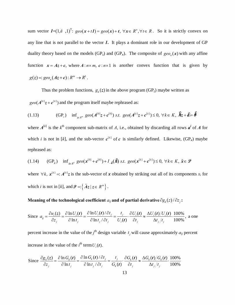
Meaning of the technological coefficient aij and of partial derivative ( ) /k jg z z∂ ∂ :
Sinceln ( ) /( ) ln ( ) ( ) ( ) ( ) 100% ,
ln ln / ( ) 100%i j ji i i i i
ijj j j j i j j j
U t tu U U U Uaz t t t U t t t
∂ ∂∂ ∂ ∂ ∆= = = = ⋅ ≈ ⋅
∂ ∂ ∂ ∂ ∂ ∆tz t t t t
t a one
percent increase in the value of the jth design variable jt will cause approximately aij percent
increase in the value of the ith term ( ).iU t
ln ( ) /( ) ln ( ) ( ) ( ) ( ) 100%Since ln ln / ( ) 100%
k j jk k k k k
j j j j k j j j
G t tg G G G Gz t t t G t t t
∂ ∂∂ ∂ ∂ ∆= = = ⋅ ≈ ⋅
∂ ∂ ∂ ∂ ∂ ∆tz t t t t
t
14
and [ ]
( ) ( ) ( ),kk ij i
i kj
g G a Uz ∈
∂= ∂
∑z t t by(1.8), a one percent increase in the value of the jth design
variable jt will cause approximately[ ]
( ) / ( ) ( ( ) / )ij i k k ji ka U G g z
∈= ∂ ∂∑ t t z percent increase in the
value of ( )kG t and approximately[ ]
( )ij ii ka U
∈∑ t absolute increase in the value of ( )kG t .
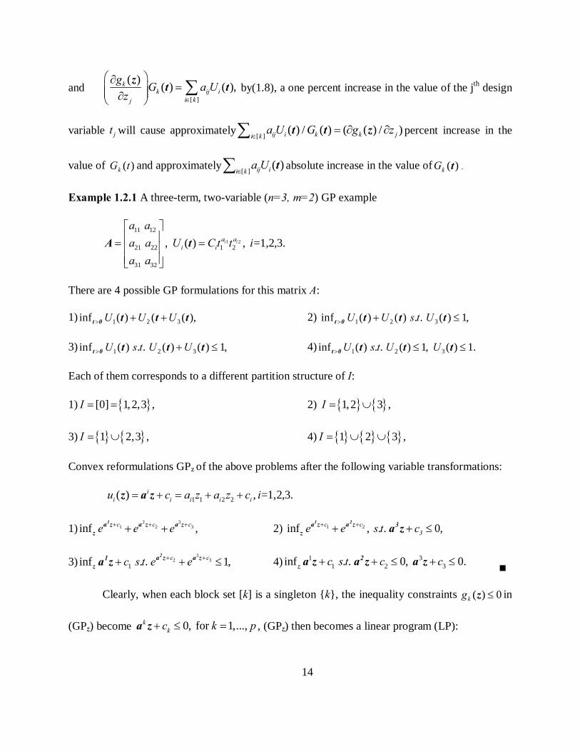
Example 1.2.1 A three-term, two-variable (n=3, m=2) GP example
1 2
11 12
21 22 1 2
31 32
, ( ) , =1,2,3.
i ia ai i
a aa a U C t t ia a
= =
A t
There are 4 possible GP formulations for this matrix A:
1) 1 2 3inf ( ) ( ( ),U U U> + +t 0 t t t 2) 1 2 3inf ( ) ( ) . . ( ) 1,U U s t U> + ≤t 0 t t t
3) 1 2 3inf ( ) . . ( ) ( ) 1,U s t U U> + ≤t 0 t t t 4) 1 2 3inf ( ) . . ( ) 1, ( ) 1.U s t U U> ≤ ≤t 0 t t t
Each of them corresponds to a different partition structure of I:
1) { }[0] 1,2,3 ,I = = 2) { } { }1,2 3 ,I = ∪
3) { } { }1 2,3 ,I = ∪ 4) { } { } { }1 2 3 ,I = ∪ ∪
Convex reformulations GPz of the above problems after the following variable transformations:
1 1 2 2 ( ) , =1,2,3.ii i i i iu c a z a z c i= + = + +z a z
1)32
31 2inf ,cc ce e e ++ ++ +1 a za z a z
z 2) 1 2inf , . . 0,c c3e e s t c+ ++ + ≤
1 2a z a z 3z a z
3)3
321inf . . 1,ccc s t e e +++ + ≤
2 a za z1z a z 4) 1 3
1 2 3inf . . 0, 0.c s t c c+ + ≤ + ≤2z a z a z a z ∎
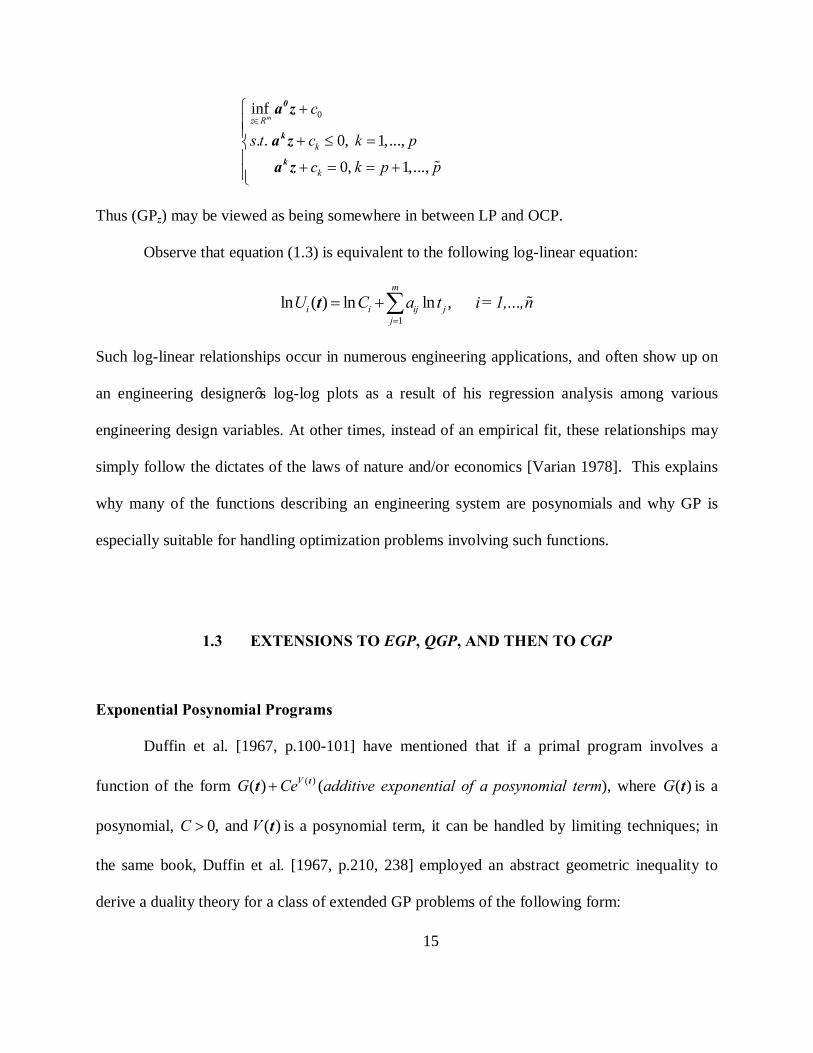
Clearly, when each block set [k] is a singleton {k}, the inequality constraints ( ) 0kg ≤z in
(GPz) become 0, for 1,...,kkc k p+ ≤ =a z , (GPz) then becomes a linear program (LP):
15
0inf
. . 0, 1,...,
0, 1,...,
mz R
k
k
c
s t c k p
c k p p
∈ + + ≤ = + = = +
%
0
k
k
a z
a za z
Thus (GPz) may be viewed as being somewhere in between LP and OCP.
Observe that equation (1.3) is equivalent to the following log-linear equation:
1
ln ( ) ln ln , m
i i ij jj
U C a t i=1,…,n=
= +∑ %t
Such log-linear relationships occur in numerous engineering applications, and often show up on
an engineering designer’s log-log plots as a result of his regression analysis among various
engineering design variables. At other times, instead of an empirical fit, these relationships may
simply follow the dictates of the laws of nature and/or economics [Varian 1978]. This explains
why many of the functions describing an engineering system are posynomials and why GP is
especially suitable for handling optimization problems involving such functions.
1.3 EXTENSIONS TO EGP, QGP, AND THEN TO CGP
Exponential Posynomial Programs
Duffin et al. [1967, p.100-101] have mentioned that if a primal program involves a
function of the form ( ) ( ) VG Ce+ tt (additive exponential of a posynomial term), where ( )G t is a
posynomial, 0, and ( )C V> t is a posynomial term, it can be handled by limiting techniques; in
the same book, Duffin et al. [1967, p.210, 238] employed an abstract geometric inequality to
derive a duality theory for a class of extended GP problems of the following form:

16
Example 1.3.1 (additive logarithm of a posynomial term)
0 10 0 0
0 11 1
, are posynomials,min ( ) ln ( ) where
, are posynomial terms . . ( ) ln ( ) 1H HH UU Us t H U
> + + ≤
t t tt t
.
Later, Lidor and Wilde [1978] treated a class of optimization problems, called Transcendental
Geometric Program (TGP), which involves posynomial-like functions whose variables may
appear also as exponents or in logarithms
(TGP) 0 inf ( ) . . ( ) 1, ,m kRG s t G k K
∈≤ ∈% %
0<tt t
where
(1.15) '[ ]( ) ( ) exp , ' , and are realsk i l lli k l
G U D t l J D∈
= ⋅ ∈ ∑ ∑% t t ,
viz., some exponential factor of a linear signomial may be multiplied to certain posynomial terms.
[Lidor, 1975] reported that the dual of the above program models chemical equilibrium problems
for non-ideal systems. The dual model they derived has the primal variables also appear in the
orthogonality conditions and thus these constraints are no longer linear and its objective value
also does not serve as a lower bound for the primal objective value, thus loses most of the
attractiveness of a dual program.
Replacing the linear signomial factors in the above model with posynomials, we get a
partial extension of the above model, which we call Exponential Posynomial Programs (EPP),
whose problem functions are of the form:
(1.16) [ ]
( ) : ( ) exp ( ) ,k i li k lG U V
∈ = ⋅ ∑ ∑t t t%
where ( ) , 0ljbl l j lj J
V D t D∈
= >∏t . Following Lidor’s terminology, we shall also call such a
function posynential. With the positivity assumption on the coefficients lD , we can easily
transform this program into a convex one:

17
(EPP)z 0 inf ( ) . . ( ) 0, m kR
g s t g k K∈
≤ ∀ ∈% %z
z z ,
with
(1.17) ( ){ }[ ]ˆ( ) : ln ( ) ln exp exp , ,i
k k i li k lg G c d k K
∈ = = + + ∈ ∑ ∑%% lz t a z b z +
where : lnl ld D= and lb is the lth row of the matrix [ ]ljB b= . We are able to derive in this thesis
a duality theory for EPP that is as powerful as the one for posynomial programs. Recall that the
problem functions ( )kg z in a posynomial program (GP)z are composites of the geometric
function ( ) ln( )ixgeo e= ∑x with affine functions iic+a z that are the log of the posynomial terms
( )iU t . Now, if we add to those affine functions a sum of exponential functions
( )exp lld∑ lb z + of the log of some other posynomial terms ln ( )lV t , we get the problem
functions for (EPP)z. This new class of programs opens a door to new area of applications such
as maximum likelihood point estimation for normal probability distribution and for some other
distributions.
Note that, upon exponentiating each of its problem functions, the above Example 1.3.1 is
equivalent to an (EPP) problem.
0 1( ) ( )10 0 1 min ( ) . . e ( ) 1H HU e s t U e−
> ⋅ ⋅ ≤t tt t t
Quadratic Posynomial Programs
The extension from GP to QGP was also prompted by a need arising from real world
applications. As noted above, the building block of GP is the posynomial term Ui(t), which is
equivalent to a log-linear relationship. In the study of Machining Economics Problem (MEP),
there is a well-known empirical tool life equation in posynomial form:

18
(1.18) 1
jm
aj
jT C t
=
= ∏
originally formulated by F.W. Taylor [1907], based on the assumption that the logarithm of the
machine tool life T is linear in the logarithms of the machining variables tj such as cutting speed,
depth of cut, feed, etc., viz.,
(1.19) 1
ln ln ln .m
j jj
T C a t=
= +∑
Using this (extended) Taylor formula, the MEP can be formulated and solved as a GP. Hough
and Goforth [1981b] hold that GP is one of the most straightforward techniques for solving the
constrained MEP, and it gives the most insight into the problem; however, this kind of
formulation of MEP had been met with limited acceptance and use by industry, mainly due to the
inaccuracy of Taylor’s tool-life equation (1.18) for some combinations of machine tools and
materials. This inaccuracy is partially attributable to the inadequacy of the linear logarithmic
assumption (1.19) for some types of MEP, (see, for example, Colding [1959, 1969]; [Colding
and Konig, 1971]; [Wu, 1964]). To correct this, they suggested adopting instead a quadratic
logarithmic assumption,
(1.20) 12
1 1 1ln ln ln ln ln
m m m
j j jl j lj j l
T C a t q t t= = =
= + +∑ ∑∑
which, after exponentiation, leads to a more accurate Colding and Wu type tool-life equation:
(1.21) 1 12 21 1
ln ln
1 1 1
m mjl l j jl lj l l
m m mq t a q ta
j j jj j j
T C t t C t= =+
= = =
∑ ∑= ⋅ =∏ ∏ ∏

19
They reported that this change increased the usage of MEP by industry. In his Ph.D. dissertation,
Hough [1978] named any finite sum of terms such as (1.21) a Quadratic Posylognomials (QPL)
and studied the following (QPL) optimization problem:
(QPL) 0 1 inf ( ) . . ( ) 1, , with =[ ] ,mm
k j jRG s t G k K t =∈
≤ ∈% %0<t
t t t
with
(1.22) 12 1
ln
[ ] [ ] 1ˆ ( ) ( ) : , .
m iij jl ll
m a q tk i i ji k i k j
G U C t k K+ =
∈ ∈ =∑= = ∀ ∈∑ ∑ ∏% %t t
The problem functions of a (QPL) are posynomial-like, except that the exponents of certain
design variables in some QPL terms ( )iU% t has an added linear function of the ln 'lt s to the usual
constants aij. Obviously, then the log of a QPL term is a quadratic function of the logarithms of
the design variables:
1 12 21 1
ln ( ) ( ln ) ln ,m m i i ii i ij jl l j ij l
U c a q t t c Q= =
= + + = + < >∑ ∑t a z + z z% ,
where [ ] , and = lni ijl m m j jQ q z t×= . Therefore a (QPL) problem can be equivalently formulated
in the z variables as:
0( ) inf ( ) . . ( ) 0, mz kR
QPL g s t g k K∈
≤ ∀ ∈% %z
z z ,
with
(1.23) { }12[ ]
ˆ( ) : ln ( ) ln exp[ , ] , ,ik k ii k
g G c k K∈
= = < > + + ∈∑%% iz t z Q z a z
which are composites of the geometric function with quadratic functions in the z variables. Of
course, if each of the above matrices iQ is symmetric and positive semi-definite (p.s.d.), (QPL)z
is a differentiable convex program, so this formulation (QPL)z is better than its predecessor
(QPL), since the hidden convexity is brought out in the p.s.d. case.

20
In practice, many nonlinear empirical formulas used in engineering optimization are
developed assuming a linear logarithmic relationship. Sometimes, a quadratic logarithmic
relationship may be more appropriate. Therefore, QPL can have applications to areas other than
MEP. When each set [k] in (1.23) is a singleton {k}, 12
ˆ( ) , , k kk kg c k K= < > + + ∀ ∈% z z Q z a z , the
corresponding model becomes a Quadratically Constrained Quadratic Program (QCQP).
Hough found that this (QPL) problem cannot be transformed into a GP problem, and
hence a second order logarithmic MEP, although more accurate, can no longer take advantage of
the powerful techniques and niceties of a GP approach. Attempting to remedy this, Hough and
Goforth [1981a,b,c] extended the theory of GP somewhat, but almost all of the niceties of a GP
approach were lost in their theory, as the authors themselves pointed out [Hough and Goforth,
1981b]:
“The QPL theory is not as powerful or as clean as the posynomial case due to the
nonlinearities and the fact that the primal variables appear in the dual (program).”
Jefferson and Scott [1985] proceeded to factor each Qi as ( )t=i i i Q B B , where Bi is a
ir m× matrix with full row rank, so 21 1 12 2 2 , ( ) || ||t t= < >=i i i iz Q z z B B z B z , where || ||⋅ is the
Euclidean norm in irR . Thus the problem functions in (QPL)z become:
(1.24) { }212[ ]
ˆ( ) ln exp || || , i ik ii k
g c k K∈
= + + ∈ ∑% z B z a z ,
which are better than those in (1.23), because more linearity is brought out. By applying
Peterson’s GGP principle to the variables-separated version of this model, they gave a
corresponding dual model and a set of optimality conditions.

21
Let us illustrate the above formulation by a very simple example.
Example 1.3.2 [Fang and Rajasekera, 1987]
12
50ln 1 10 1 2 1 1 2
1/21 1 2
inf ( )( ) ,
. . ( ) 0.01 1,
t
RG t t t t t
QPLs t G t t
− −
∈ = ⋅ +
= + ≤
%0<t
t
t
This is a (QPL) problem, since the log of its first term has a quadratic term 2 11
1 250 ,z = < >z Q z
with [ ] [ ]1 1 1 1 1 1 2 21 1 112 2 2
1010 0 10 0
0
100 0( ) , so , || || (10 )
0 0TQ B B B z = = = = < >= =
z,Q z B z . ∎
Composite Posynomial Programs (A unified model for both EPP and QPL)
The problem functions for (QPL)z (1.23) and for (EPP)z (1.17) are respectively:
{ }12[ ]
ln exp ,iii k
c∈
+ + < > ∑ ia z z Q z and ( ){ }[ ]
ln exp expii li k l
c d∈
+ + ∑ ∑ la z b z +
An obvious extension to both EPP and QPL models is to use a general convex function
: mi R R→h as the last term in the above expression to obtain more general problem functions
(1.25) { }[ ] ( ) : ln exp[ ( )]i
k i ii kg c
∈= + +∑z a z h z%
for the resultant Composite Posynomial Program (CPP)z
(CPP)z
0inf ( ) . . ( ) 0, m kR
g s t g k K∈
≤ ∀ ∈% %z
z z ,

22
1.4 THESIS PLAN
The intended research here is to develop for EPP, QPP, and CPP a unified basic duality theory
which is in parallel with those basic duality theorems of GP contained in Chapter 4 of [Duffin et
al., 1967].
These have 3 major elements:
a) The main lemma of GP, which is the basis for proving all other duality theorems,
b) The first duality theorem of GP, which asserts the existence of a dual optimal solution
under mild conditions on the primal problem, and
c) The second duality theorem of GP, which asserts the existence of a primal optimal
solution under mild conditions on the dual problem.

23
2.0 LITERATURE REVIEW ON DUALITY THEORY
Duality theory is essential for establishing optimality conditions, for performing
sensitivity (post-optimality) analysis. It also provides insight into the optimization problem and
a meaningful economic interpretation of the model. It infers about the relationships between the
primal and the dual optimal objective values. The importance of LP duality was first emphasized
by [Dantzig, 1965, Chapter 6], and that of Conic duality for Convex Programs (reformulated in
conic form so that the potential reduction interior-point methods would apply) by [Nesterov and
Nemirovski, 1994, Section 4.2] and by [Ben-Tal and Nemirovski, 2001, Lecture 2].
The celebrated duality theory of LP developed by [Gale-Kuhn-Tucker, 1951] has served
as a model for all subsequent developments in more general settings. The first such extension by
Fenchel to convex programs without explicit (nonlinear) constraints can be found in
[Rockafellar, 1970, Section 31]. The duality theory of GP is somewhere in between the duality
theories of LP and of OCP. Equation Chapter 2 Section 1
2.1 DUAL PROGRAM GD AND DUALITY THEORY OF GP
In this section we shall review the duality theory for the GP problems studied by Duffin
and Peterson [1966]. These problems are stated below and they belong to a special case of our

24
earlier GP model (1.2) in Section 1.2 under the assumption that , ,n n I I= = %% and [ ] [ ]= % %A C A C ,
i.e., no monomial equality constraints are considered.
Primal posynomial program (GP)
(GP) { }0inf ( ) . . ( ) 1, : 1, ,m k
RG s t G k K p
∈≤ ∈ =
<tt t L
0, where ( )kG t are as given in (1.4).
As a special case of (1.9) we have
An equivalent convex reformulation of (GP)
(GP)z
0inf ( ) . . ( ) 0, m kR
g s t g k K∈
≤ ∀ ∈z
z z , where ( )kg z are as given in
Error! Reference source not found., and
1=ln ( ) ln ln , [ ] , = ln , : ln ,mi i i ij j j j j j i ij J
c U C a t z z t c C=∈+ = + = =∑ia z t z and ia =ith row of A.
Likewise, as a special case of (1.14) we have
A GGP formulation of GP
(2.1) (GP)x 0 0 inf ( ) . . ( ) 0, ,n
k k
Rgeo s t geo k K
∈+ + ≤ ∀ ∈ ∈
xx c x c x P ,
where { } | m nR R= ∈ ⊂Az zP is the column space of A, [ ] [ ][ ] , =: , [ ]k ki i k i i i kx x i I c∈ ∈= ∈ =ix a z, c ,
and [ ]
( ) : ln[ exp ] : knkii k
geo x R R∈
= →∑x is the geometric function (also called logexp(x))
defined in Section 1.2.
So one has
{ }[ ]( ) ln exp( ) ( ) ln ( )k k
i i k ki kgeo x c g G
∈+ = + = =∑x c z t
The variables in ( )k kgeo +x c are separated for different ˆk K∈ .
[Duffin and Peterson, 1966] defined the dual program GD for the primal program GP as
follows (note that each primal term iU is assigned a dual variable iδ ):

25
Dual posynomial program (GD) under the convention that 00=1.
(2.2) (GD)
( )ˆ [ ]
0
1
[ ]
sup ( ) : (Dual function)
. . 0, , 1 (normality condition)
0, (orthogonality conditions)
where : ,
i
ni k ik K i k
R
in
ij ii
k ii k
V C
s t i I
a j J
δλ δ
δ λ
δ
λ δ
∈ ∈∈
=
∈
=
≥ ∀ ∈ =
= ∀ ∈
= ∀
∏ ∏
∑
∑
δδ
ˆ .k K
∈
Observe that ( )1 1
( ) 0i k
pn
i i ki k
V C δ λδ λ= =
= >∏ ∏δ for all ≥ 0δ . We set ( )sup GD 0= , if (GD)
is infeasible.
The meaning of the orthogonality conditions in (GD)
In vector form, they are expressed as:
0, j j J⋅ = ∀ ∈a δ , where ja is the jth column of the matrix A,
and in matrix form:
( ( ) = )T i Tii I
A δ∈
= ⇔ ⊥ ⇔ ∑δ 0 δ a 0P .
So these orthogonality conditions may be summarized as
( )⊥∈δ D = P .
Thus the orthogonality conditions in (GD) can be obtained simply by taking the orthogonal
complement of the primal space P in (GP)x. Moreover,
(2.3) 0, ,⋅ = ∀ ∈ ∀ ∈x δ x δP D
The space D is also called the dual space of the program (GD).

26
The dimension of the dual feasible set (= nR+ ∩ ∩D normality hyperplane, called dual flat)
is termed the degree of difficulty of the dual program (GD) in the geometric programming
literature. This number is dd=n-m-1, when A is of full column rank m.
The concavity of the log-dual function in (GD) [Duffin et al. 1967, p. 121]
The log-dual function
(2.4) ( )0 [ ] 1 1
( ) : ln ( ) ln / ( ln ) lnp pn
i i k i i i i k kk i k i k
v V C cδ λ δ δ δ λ λ= ∈ = =
= = = − + ∑ ∑ ∑ ∑δ δ
is concave on its domain of definition.
Thus the dual program (GD) is equivalent to an ordinary convex program. Note that
min ( ) max ( ) max ( ) min1/ ( )v v V V− ⇔ ⇔ ⇔δ δ δ δ ,
and that ( ) 1 / ( ) vV e−= δδ is convex. Unlike the primal problem, the log-dual function ( )v δ is not
differentiable. In fact, it is not even continuous, since its domain has an empty interior due to the
normality condition. Its partial derivatives exist only when 0iδ > :
(2.5) ln 1, [0]( )ln ln , [ ], K
i i
i i ki
c ivc i k k
δδ λδ
− − ∀ ∈∂= − + ∀ ∈ ∈∂
δ
In general, the λk’s in (GD) are treated as dependent variables, and the dual objective V(δ)
as a function of δ alone. Computationally, [Dembo, 1978a, p.232] feels this is a very bad
practice, as it obstructs the design of efficient and numerically stable software for (GD). He
holds that for computational purposes, both the λk’s and δi’s should be regarded as independent
variables, and thus the log-dual v(�, �) becomes a separable function.
Observe that the term coefficients Ci and the exponents aij in (GD) are separated in that
the former appear only in the objective and the latter only in the (linear) constraints; whereas in

27
(GP) they are scattered all over the terms ( )iU t of the functions ( ).kG t In summary, through the
use of (GD), one can recover 3 exploitable structures: linearity, separability, and convexity
which are originally hidden in the (GP) model. The founders of GP first pointed out these
unique advantageous features.
Basic duality theorems of GP
These have three major components:
0) The main lemma of GP, which is the basis for proving all other duality theorems,
1) The first duality theorem of GP, which asserts the existence of a dual optimal solution
under mild assumption on the primal problem, and
2) The second duality theorem of GP, which asserts the existence of a primal optimal
solution under mild assumption on the dual problem.
Duffin and Peterson [1966] first developed a duality theory for posynomial GP based on
a so-called geometric inequality, which is the only machinery needed to derive the dual program
GD and to establish the main lemma of GP. This key lemma provided weak and incipient
duality relationships between the primal and the dual GP programs.
The Geometric Inequality
It is a slight generalization of the classical arithmetic mean−geometric mean (AGM)
inequality. This AGM inequality is stated and proved in any book on inequalities, e.g.
[Beckenbach and Bellman, 1965], and [Hardy, Littlewood, and Polya, 1952, pp.17-18]. Its strict
version is equivalent to the strict convexity of the exponential function exp x, and also equivalent
to the strict concavity of the logarithmic function ln x. For easy reference, we list below some
forms of the AGM inequality and the geometric inequality, and provide proofs in Appendix A.2.
28
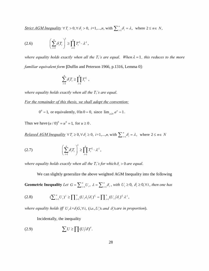
Strict AGM Inequality 1
0, 0, =1,..., , with , where 2 ,ni i ii
T i n n Nδ δ λ=
∀ > ∀ > = ≤ ∈∑
(2.6) 1 1
i
nn
i i ii i
T Tλ
δ λδ λ= =
≥ ⋅ ∑ ∏ ,
where equality holds exactly when all the Ti’s are equal. When 1λ = , this reduces to the more
familiar equivalent form [Duffin and Peterson 1966, p.1316, Lemma 0]:
1 1
i
nn
i i ii i
T T δδ= =
≥∑ ∏ ,
where equality holds exactly when all the Ti’s are equal.
For the remainder of this thesis, we shall adopt the convention:
00 0 1, or equivalently, 0 ln 0 0, since lim 1a
a a↓= = = .
Thus we have 0 0( / 0) 1, for 0u u u= = ≥ .
Relaxed AGM Inequality 1
0, 0, =1,..., with , where 2ni i ii
T i n, n Nδ δ λ=
∀ ≥ ∀ ≥ = ≤ ∈∑
(2.7) 1 1
i
nn
i i ii i
T Tλ
δ λδ λ= =
≥ ⋅ ∑ ∏ ,
where equality holds exactly when all the Ti’s for which 0iδ > are equal.
We can slightly generalize the above weighted AGM Inequality into the following
Geometric Inequality Let1 1
, n ni ii i
G U λ δ= =
= =∑ ∑ , with 0, 0,i iU iδ≥ ≥ ∀ , then one has
(2.8) 1 1 1
( ) ( ) ( ) ,i in nn
i i i i ii i iU U Uδ δλ λλ δ δ λ
= = =≥ =∑ ∏ ∏
where equality holds iff = , , ( . ., 's 'si i i iU G i i e U andλ δ δ∀ are in proportion).
Incidentally, the inequality
(2.9) ( ) .U U δδ≥∑ ∏

29
that appears on the front cover of the first textbook on GP [Duffin et. al. 1967] is the special case
(omitting indexes) of the above formula(2.8) for 1λ = .
The original version of this inequality [Duffin and Peterson 1966, p.1316, Lemma 1]
requires that 0,iU i> ∀ . Under this assumption, by setting ,ixiU e i= ∀ , taking logarithm of its
two sides and rearranging terms, one obtains an equivalent form of (2.8) [Duffin et. al. 1967]:
(2.10) ( ) ln( / ) ( ) ln lni i i igeo geoλ δ δ λ λ δ δ λ λ+ = + − ≥ ⋅∑ ∑x x x δ ,
where ( ) : ln( )ixgeo e= ∑x , as was already defined in section 1.2, and by our convention,
ln( / ) ( | ), when =0i i iδ δ λ λ=∑ δ 0 . This inequality becomes an equality iff ( / ) ,ix
i G e iδ λ= ∀ .
Lemma 2.1.0 (Main Lemma of GP) If t is feasible for primal program (GP) and δ is feasible for
dual program (GD), then
0 ( ) ( ).G V≥t δ
Moreover, under the same conditions 0 ( ) ( ),G V=t δ if, and only if, the following set of
extremality conditions holds:
(2.11) 0( ) ( ) , [0] (1)( ), [ ], (2)
ii
k i
U G iU i k k K
δλ
∈= ∈ ∀ ∈
t tt
in which case t is optimal for primal program (GP) and δ is optimal for dual program (GD).
A primal geometric program (GP) is said to be superconsistent if
. . ( ) 1, .ks t G k K∃ > < ∀ ∈t 0 t The original Lagrangian for (GP) is defined to be the function
0( , ) : ( ) [ ( ) 1], defined for in and m po k kk K
L G G R Rµ +∈= + − > ∈∑t μ t t t 0 μ ,
A saddle point of the original Lagrangian ( , )oL t μ is a point ( )t', μ' that satisfies:
0
max ( ', ) ( ', ') min ( , ')o o oL L L>≥
= =t 0μ
t μ t μ t μ

30
Theorem 2.1.1 (First Duality Theorem of GP): Suppose that the primal program (GP) is
superconsistent and has a minimum solution t’, then there exists a Lagrange multiplier vector
pR+∈μ' for t' such that ( )t', μ' forms a saddle point for ( , )oL t μ , and the dual program (GD)
also has a maximum solution 'δ with 0' : '/ ( )G=λ μ t' such that
0min(GP) ( ') ( ') max(GD)G V= = =t δ
Moreover, each pair of primal and dual optimal solution ( )t',δ' satisfies
(2.12) ' '
' ' '
( ), [0]( )
, [ ], , and 0i
ii k k
V iU
i k k Kδ
δ λ λ
∈= ∈ ∈ >
t'δ
A dual program (GD) is said to be canonical if there exists a positive vector δ > 0 in the
dual space D. One can also assume without loss of generality that this dual vector δ is feasible.
Theorem 2.1.2 (Second Duality Theorem of GP): Suppose that primal program (GP) is
consistent and dual program (GD) is canonical. Then primal program (GP) has a minimum
solution t’.
Let us use an example to show why sometimes it is easier to solve a primal GP through
its dual GD without the need of calculating derivatives.
Example 2.1.1 A two-term, one-variable (n=2, m=1) GP example
1 21 20
inf a a
tC t C t−
>+ , where all parameters: 1 2 1 2, , ,C C a a are positive.
Solution The dual program is
2
1 21 2sup 1 2R
C C
δ
δ δ
δ δ+∈
s.t. 1 2 1 δ δ+ = ; 1 1 2 2- 0a aδ δ+ =

31
The exponent matrix and a unique dual solution are given (respectively) by
1
2
aa
−
and 1 2 1 2
2 1 1 2
/ ( ) / ( )a a aa a a
δδ
+ = +
From the extremality condition(2.11) (1), we see that
* *1 1* *2 2
( )( )
UU
δδ
=tt
, thus 1 2( )2 1
1 2
a aa C ta C
− += , 1 2 1 1
2 2
a a C atC a
+ = , so 1 2
1
* 1 1
2 2
a aC atC a
+ =
.
This example has an application to a simple inventory control problem [Nahmias, 1989,
p.147-148]. Consider 1
0inf ( ) / 2 ,Q
G Q K Q hQ cλ λ−
>= + + where C1=Kλ, C2=h/2, a1=a2=1,
λc=constant, so the economic order quantity (EOQ) is
* 2 /Q K hλ= . ∎
According to Peterson [2001a], the birth of GP occurred in Pittsburgh in 1961 at
Westinghouse R&D, when Zener [1961] discovered a simple formula for the minimum value of
a posynomial cost function whose number of terms exceeds the number of design variables by
just one. Zener’s approach was initially based on Fermat’s principle in calculus, namely, set the
first partial derivatives to zero and solve; however, instead of solving directly for these design
variables, he associated with each term a new variable representing its relative contribution in the
total cost function, and solved the problem completely in this zero degree of difficulty case—we
give a detailed description of his approach in Appendix B.

32
2.2 ASSESSING A DUAL APPROACH TO GP
In this section, we list the advantages and disadvantages of a GP dual approach.
Dual to Primal conversion of optimum solutions
When there is perfect duality, taking logarithms of both sides of equation (2.12) gives
(2.13) ( )1
ln( ( )), i [0]ln , i [ ], for which 0
mi
ij j ij i k k
Va z c
k k Kδδ λ λ=
∈+ = ∈ ∈ >∑
δ
where ic :=lnCi, i=1,…,n and zj:=lntj, j=1,…,m.
The niceties of a GP dual approach
1. The primal problem generally has highly nonlinear constraints even in its convex form (GPz),
whereas the dual problem has only linear constraints. This is a clear advantage, since linear
constraints are much easier to handle than are nonlinear constraints in developing numerical
methods for solving optimization problems.
2. The above advantage becomes more apparent when one is to solve large-scale GP problems,
because the often present sparsity structure of the exponent matrix A can be handled more
directly in (GD) than in (GP).
3. The dual problem, just like the primal one, is also a convex program.
4. The dual to primal conversion only involves solving a system of linear equations(2.13),
which is computationally easy. This is possible as long as there are enough indices k for
which 0kλ > in(2.13).

33
The drawbacks of a GP dual approach
1. The log-dual objective function1 1
( ) ( ln ) lnn pi i i k ki k
v cδ δ λ λ= =
= − +∑ ∑δ is only differentiable
at points where 0> δ , since ( ) / , as 0i iv δ δ +∂ ∂ → +∞ →δ . So if the optimum dual solution
has some zero components, any gradient-based numerical code may fail to find this optimum
solution.
2. There may not be enough indices k such that 0kλ > in order to solve for z in(2.13) (this
happens when there are too many primal forced constraints in GP being slack at optimum),
and solving the subsidiary problems may be cumbersome.
Some remedies for a GP dual approach
1. Fang et.al. [1988] implemented a well-controlled dual perturbation method for (GP)
which guarantees to overcome the non-differentiability difficulty and the dual-to-primal
conversion is via solving a simple LP.
2. Rajgopal and Bricker [2002] also proposed a generalized LP algorithm for (GP) which
avoids all of the computational difficulties mentioned above.
Sensitivity (or Marginal) Analysis of the Optimum Objective Value in GP
The optimum solutions to (GP) and to its dual (GD) each provide sensitivity information
of the optimum value to the parameter changes. To see this, we perturb each problem function
( )kG t by dividing it by a positive amount Bk (with B0=1), the corresponding log-dual objective
becomes:
(2.14) ( )0 [ ] 1 1
( ) ln / ( ln ) (ln ),p pn
i i k i k i i i k k kk i k i k
v C B c bδ λ δ δ δ λ λ= ∈ = =
= = − + − ∑∑ ∑ ∑δ

34
(where : lnk kb B= ) while subject to the same dual constraints as before [Dembo, 1982, p.3]. We
define the log-dual Lagrangian function [Dembo, 1978b, p.334]:
0 0 0 1 1( , , ) : ( ) ( 1) ( )m n
ij i jj il z v z a zλ δ
= == + − + ∑ ∑zδ δ
which is simply equal to ( )v δ at any dual feasible point δ. Now suppose that z* and (δ*, λ*) are
respectively optimum solutions to the perturbed pair of GP problems and there is no duality gap.
Then in the neighborhood of optimum solution satisfying some conditions specified in
[Dembo, 1982, pp.7-8, pp.15-16, Table 3], we have
(2.15)
* * * *0 0
* * * * * * * *0 0 1 1
1 1
( ) ( ) ( , , )
( ln ) (ln ) ( 1) ( )pn m n
i i i k k k ij i jj ii k
g v l z
c b z a zδ δ λ λ λ δ= =
= =
= =
= − + − + − +∑ ∑ ∑ ∑
*z zδ δ
.
(2.16) * * *
* * * *0 0 0( ) ( ) ( ), , i k i ji k ij
g g g zc b a
δ λ δ∂ ∂ ∂= = − =
∂ ∂ ∂z z z
This information provides a quick estimate of the changes in optimum value of (GP),
should there be a slight change in the parameter values:
• If the right hand side of the constraint ( )k kG B≤t increases by 1%, the minimum value of
(GP) will decrease by about *kλ %; if the term coefficient Ci increases by 1%, the
minimum value of (GP) will increase by about *iδ %; and if the exponent aij increases by 1
(and * 1jt > ), the minimum value of (GP) will increase by about * *i jzδ %. In practice, the
exponents are usually fixed by the laws of nature and/or economics.
• If, for a fixed k, all term coefficients Ci, i∈[k], increase by 1%, the value of *( )kG t also
obviously increases by 1%. By the first formula in(2.16), the minimum value of (GP)

35
should increase by about * *[ ] i ki k
δ λ∈
=∑ %. This is trivially confirmed, if k=0, since *0 1.λ =
For k>0, we argue as follows:
* *(1.01) ( ) ( ) / (1.01) (0.99)k k k k kG B G B B≤ ⇔ ≤ ≈t t
(by a first order Taylor approximation: 1(1 ) 1 , for 0x x x−+ ≈ − ≈ ). Then by the second
formula in(2.16), decreasing Bk by 1% will cause the minimum value of (GP) increase by
about *kλ %. This shows coherence between the first two formulae in(2.16). A similar
result also holds between the first and the third formulae: Increasing the exponent aij by 1
amounts to multiplying the ith term coefficient Ci by *jt , or equivalently, to adding ci by *
jz
* *since ln( )i j i jC t c z= + , which, according to the first formula in(2.16), will in turn gives
about * *i jzδ % increase in the minimum value of (GP).
2.3 FENCHEL’S DUALITY THEORY AND GENERALIZED GEOMETRIC
INEQUALITY
In the previous two sections we have briefly reviewed the basic duality theory for the
prototype GP. Our aim in this thesis is to establish similar basic duality theories for the extended
GP cases. We have seen that the dual objective of GD and the main lemma can be derived solely
by applying the geometric inequality(2.8). However, in section 1.3, we have also noted that this
same approach was not successful for the EGP and QGP cases. In order to develop useful dual
programs and the main lemma for these extended GP cases, we need to, first of all, assign
additional dual variables to each second tier posynomial term in the primal program, and then

36
utilize generalized geometric inequalities instead of just geometric inequality. In fact, even for
the prototype GP, it is still beneficial to look at its duality theory from the perspective of
Fenchel’s conjugate transform. Specifically, the dual objective of (GD) is the exponential of the
negative of the conjugate transform of the Lagrangian of the primal program (GP)x, and the
main lemma can be derived from the conjugate inequality for this Lagrangian and its conjugate
transform. We shall see this after we prove Lemma 3.0. In this section we will first introduce
Fenchel’s conjugate transform that transforms an extended-real-valued function : nf R R→ ,
where : { } [ , ]R R= ∪ ±∞ = −∞ +∞ , into another function of the same type. We often find it more
convenient to work with functions of this sort when dealing with optimization and conjugate
duality. Below we use two examples to explain why.
Following (1.1), we consider an inequality-constrained program (P):
(2.17) (P) 0inf { ( ) | ( ) 0, , } : inf( ),n kx Rf x f x k K x C P
∈≤ ∈ ∈ =
where ˆ{1, , }, , : , : {0} ,nkK p C R f C R k K K= φ ≠ ⊂ → ∀ ∈ = ∪L and the feasible set S is defined
via { }: ( ) 0, kS C f k K= ∈ ≤ ∀ ∈x x .
Note that if we define iS to be the indicator of S, then this program (P) can be identified with its
objective function 0: Sf f i= + in the sense that inf(P) = infS f0 = inf f, and argmin(P) = argminS f0
= argmn f. This function f is from nR to ( , ]−∞ +∞ . Another example is the optimal value (or
perturbation) function of (P):
(2.18) 10( ) : inf { ( ) | ( ) , , }, for : [ ]n
kk k k px R
v f x f x b k K x C b =∈
= ≤ ∈ ∈ =b b .
This function v is from to [ , ]pR −∞ +∞ .
Extended-real line R and extended-real-valued functions on nR : some terminology

37
Just like the real line R , the extended real line R , is also a linearly (or totally) ordered set:
any two elements x and y in Rare comparable, i.e. either or x y y x≤ ≤ . It is also equipped with
2 additional conventions:
1. ∞ − ∞ = ∞ = −∞ + ∞ (Inf-addition rule). 2. 0 ( ) 0 ( ) 0⋅ ±∞ = = ±∞ ⋅ .
The first rule is not symmetric, because we orient toward minimization. The implications of
these rules are listed in Appendix C. Unlike in R , every subset C in Rhas in Ra supremum
supC and an infimum inf C . (Caution: inf and sup -φ = ∞ φ = ∞ , so that inf sup !φ > φ ).
In general, we use the capital letter F to denote the effective domain dom f of a function
: nf R R→ , that is, { }dom := | ( )nF f x R f x= ∈ < ∞ , and we shall call f proper if it is never -∞
and F ≠ φ , and improper if otherwise. So a proper function f is finite-valued on F ≠ φ but =∞
elsewhere, and an improper one is somewhere -∞ or everywhere + ∞. For instance, the support
function of C defined by { }( ) ( | ) : sup | CS y S y C y x x C= = ⋅ ∈ for any set C in nR , and the
indicator function of , CC i are both proper, when C is nonempty. When C is empty, however,
they are both improper, , i Sφ φ≡ ∞ ≡ −∞ . The objective function f of the above program (P) is
improper exactly when program (P) is inconsistent, i.e. f S≡ ∞ ⇔ = φ , and its perturbation
function v is improper: ( )v = −∞b when (P) has an unbounded infimum for some perturbation
vector b. Proper functions are our central concern, but improper ones such as the above
examples do arise indirectly and hence cannot be ruled out from our consideration. The sum of
two proper functions f and g is proper exactly when F G∩ ≠ φ , or else f g+ ≡ ∞ . For a function
: nf R R→ , we also define

38
the epigraph of f, { } epi : ( , ) | ( )nf x R R f xα α= ∈ × ≤ ,
the strict epigraph of f, { } epi : ( , ) | ( )s nf x R R f xα α= ∈ × < ,
the hypograph of f, { } hpo : ( , ) | ( )nf x R R f xα α= ∈ × ≥ ,
the strict hypograph of f, { } hpo : ( , ) | ( )s nf x R R f xα α= ∈ × > ,
the (lower) level set of f, { }: | ( ) nf x R f xα α≤ = ∈ ≤ , which corresponds to a ‘horizontal
cross section’ of epi f, and other similar level sets such as ,f fα α< = , etc. For example, the level
set of the objective function f of the above program (P) (2.17) is
(2.19) 0 00 1 pf C f f fα α≤ ≤ ≤ ≤= ∩ ∩ ∩ ∩L
The Minkowski sum of any two sets C, D in Rn is the set : { | , }C D x y x C y D+ = + ∈ ∈ ,
and the multiple of C by a scalar t in R is the set : { | }, ( 1)tC tx x C C C= ∈ − = − . The Cartesian
product of two sets ,n mC R D R⊂ ⊂ is denoted (C, D). We will simply write ( , ) for ( ,{ })C y C y
and likewise, if n=m, for { }C y C y+ + . Clearly, ( )t C D tC tD+ = + , but for any scalars r and s,
one generally has ( )r s C rC sC+ ⊂ + only, the reverse inclusion may fail as is evidenced by the
set C={-1,1}and scalars r=s=1. Note that 0 C D C D∈ − ⇔ ∩ ≠ φ , and
0 0C x x C x C∈ − ⇔ ∈ − ⇔ ∈ .
A set C is convex if (1 ) , (0,1)t C tC C t− + ⊂ ∀ ∈ (the reverse inclusion trivially holds).
The sum, scalar multiple, and arbitrary intersection of convex sets are again convex sets. For a
convex set C and non-negative scalars 0, 0, ( )r s r s C rC sC≥ ≥ + = + , thus C+ C =2C, C+ 2C
=3C, etc.; if, in addition 0 , then 0C r s rC sC∈ ≥ ≥ ⇒ ⊃ . A set C is a cone if 0 , andC∈
, 0tC C t⊂ ∀ > . A set K is a convex cone if it is both a cone and a convex set. For a nonempty

39
set K, this condition is equivalent to ,R K R K K+ ++ ⊂ and also to , R K K K K K+ ⊂ + ⊂ , where
R+ denotes the set of all non-negative reals.
A function : nf R R→ is convex if for all points 0 1,x x in F and scalar t in (0, 1), f and
0 1: (1 )tx t x tx= − + satisfies Jensen’s inequality:
(2.20) 0 1( ) (1 ) ( ) ( )tf x t f x tf x≤ − + .
f is concave if its negative –f is convex. The (lower) level sets and f fα α≤ < , epigraphs epi f and
strict-epigraphs epis f of a convex function f are convex. A function : nh R R→ is positively
homogeneous (ph) if h satisfies
0 , ( ) ( ), , 0H h tx th x x H t∈ = ∀ ∈ ∀ > . (Thus (0) 0 or -h = ∞ )
It is sublinear if in addition
0 1 0 1 0 1( ) ( ) ( ), ,h x x h x h x x x H+ ≤ + ∀ ∈ (Subadditivity)
Equivalently, a sublinear function is one which is both ph and convex. As an example, the
support function of any subset C is sublinear.
It is easy to show that a function : nf R R→ is convex (respectively: ph, sublinear) iff
its epigraph epi f is a convex set (respectively: a cone, a convex cone) in nR R× .
We denote ri (S) the relative interior of any set S in nR .
Proposition 2.3.0 [Rockafellar, 1970, Theorem 7.2] If a convex function : nf R R→ is
somewhere −∞ , it is everywhere −∞ on the relative interior of its domain ri (F); hence a convex
function that is somewhere finite on ri (F) must be proper.
Proposition 2.3.1 (convexity in composition) [Rockafellar and Wets, 2004, Exercise 2.20 (c)]
Suppose (F,G): Rn→Rm×Rl is a mapping (where m≥0, l≥0) such that each of the m components of

40
F is a convex function and each of the l components of G is an affine function, and
: m lh R R R× → is a convex function that is nondecreasing in its first m components. Then the
composite function ( ) : ( ( ), ( )) : nf x h F x G x R R= → is convex. (In particular, if
0, ( ) ( ( ))l f x h F x= = , and if 0, ( ) ( ( ))m f x h G x= = .
Lower semicontinuity of a function
A function : nf R R→ is continuous at x if | | 0 ( ) ( )y x f y f x− → ⇒ → . The lower and
upper limits of f at x are respectively defined by
(2.21) | | 00 | |
( ) lim inf ( ) : sup inf ( ), ( ) lim sup ( ) : inf sup ( )y x y x t tt y x y x t
f x f y f y f x f y f y→ − ≤ >> → − ≤
= = = = .
Clearly, one has ( ) ( ) ( ), at any , , and , for - .f x f x f x x f g f g g f≤ ≤ = − = − = We say f is
lower semicontinous (lsc) at x if ( ) ( )f x f x= , upper semicontinous (usc) at x if ( ) ( )f x f x= . It
can be shown that f is continuous at x iff f is both lsc and usc at x iff both f and –f are lsc (or usc)
at x. If we let { }( ; ) : | with ( )i iL f x R x x f xα α= ∈ ∃ → → , then ( ) and ( )f x f x are respectively
the smallest and largest element in the set ( ; )L f x and
(2.22) { } { }( ), ( ), ( ) ( ; ) [ ( ), ( )] : | ( ) ( )f x f x f x L f x f x f x R f x f xα α⊂ ⊂ = ∈ ≤ ≤ .
(Semi-) continuity on nR means the property holds everywhere in nR . Lower semicontinuity on
nR can be characterized as follows:
Proposition 2.3.2 The following properties of a function : nf R R→ are equivalent:
(a) f is lsc on nR ;
(b) epi f is closed in nR R× ;
(c) f α≤ is closed is , nR Rα∀ ∈ .

41
For instance, the support function of any subset C is lsc; and in the program (P)(2.17), if the set
C is closed, and all the problem functions ˆ,kf k K∈ are lsc, then (2.19) shows the objective
function f for program (P) is also lsc.
The closure, interior, and complement of a set S of nR are respectively denoted by cl S,
int S, and SC. For any function : nf R R→ , one has cl (epi f) = [int (hpo f)] C = epi ( f )
[Rockafellar and Wets, 2004, Exercise 1.13]. This condition implies that the lower limit function
f is the largest lsc function g not exceeding f, also called the lower semi-continuous hull or the
(lower) closure of f, and is denoted by cl f; thus
( ) cl epi epi(cl ), and cl ( ) ( ) liminf ( )y x
f f f x f x f y→
= = =
Proposition 2.3.3 Let : nf R R→ be any function. If f is improper, so is cl f; if f is proper
convex, so is cl f. [Rockafellar, 1970, Theorem 7.4]
The (closed) convex hull, (cl) con f of a function f is defined to be the largest (lsc) convex
function g not exceeding f. Clearly:
cl con {cl , con }f f f f≤ ≤ .
For any lsc convex (respectively, lsc, convex) function g, g f≤ is equivalent to cl con g f≤
(respectively, cl f, con f).
A key duality result in convex and variational analysis is the following
Theorem 2.3.4 (envelope representation of convex sets and convex functions) [Rockafellar and
Wets, 2004, theorem 6.20 and 8.13]
1). A nonempty closed convex set in nR is the intersection of its supporting half-spaces, hence is
the intersection of a family of closed half-spaces.

42
2). An lsc proper convex function : nf R R→ is the pointwise supremum of its affine supports,
hence is the pointwise supremum of a family of affine functions.
Remark An immediate consequence of this, in view of Proposition 2.3.3, is that any proper
convex function must have at least one affine support, and hence one affine minorant.
Fenchel’s Conjugate Inequality for a Function and its Conjugate Transform
The (Fenchel) conjugate of any function : nf R R→ is another function * : nf R R→
(2.23) *, , ,( ) : sup [ ( )] sup { ( ) | ( ) }, where ( ) :x x x xf y y x f x l y f x l y x yα α αα α= ⋅ − = ≤ = ⋅ −
Hence *,( , ) epi
epi epi xx ff l αα ∈
= ∩ , and
{ } { },epi ( , ) | ( , ) | ( , 1) ( , )nxl y R R x y y x yα β α β β β α= ∈ × ⋅ − ≤ = − ⋅ ≤
The latter sets are closed half-spaces. So *epi f is a closed convex set and f* is an lsc convex
function. It may be improper due to 2 reasons:
(2.24) ( )*
*
a) is somewhere hence everywhere , and this happens exactly when .
b) is everywhere , and this happens exactly when has no affine minorant, as
f f
f f
− ∞ ≡ ∞
∞
(2.25) ( )*,( ), ( ) : ( ),yf y y x f x x f x y x l x xββ β β≥ ⇔ ≥ ⋅ − ∀ ⇔ ≥ ⋅ − = ∀
e.g. the proper function ( ) | |, f x x x R= − ∀ ∈ has no affine minorant and *f ≡ ∞ .
Proposition 2.3.5 For any function : nf R R→ , one has
(2.26) * * * *(cl ) (con ) (cl con )f f f f= = =
Proof Since an affine function is lsc convex, it minorizes f iff it minorizes any one of these 3
functions: cl f, con f, cl con f. The above equation then follows from (2.25) . ∎

43
The conjugate of the indicator function iC of any set C in nR is the support function SC of
C. When C is a cone, then C CS i −= , and the barrier cone of C, domC CB S= equals its polar cone,
C− . The conjugate of the geometric function, ( ) ln( )ixgeo e= ∑x , is the entropy function
( ) : ln , if 0, 1i i i ient y y y y= ≥ =∑ ∑y , and := ∞ if otherwise (Where 0 ln 0 0= ). Trivially, one
has *(0) inff f− = . So inf (0)geo ent= − = −∞ and this can be approached by letting ix → −∞
in geo(x) for each i. The mapping *f f→ is called the (Legendre-) Fenchel transform. It is
obviously order-reversing * * f g f g≤ ⇒ ≥ .
The following result is an analogue of proposition 2.3.3.
Proposition 2.3.6 Let : nf R R→ be any function. If f is improper, so is f*; if f is proper
convex, so is f*. [Rockafellar, 1970, Theorem 12.2]
Proof The first part is easy. For the second part, if f is proper convex, the remark following
Theorem 2.3.4 shows that f has at least one affine minorant, hence by (2.24) (b), f* is not
everywhere ∞ ; on the other hand, since f is not everywhere ∞ , by (2.24) (a), f* is never −∞ . Thus
f* is also proper. ∎
The subdifferential (or set of subgradients) of a proper function f at a point x is the set
(2.27) { }( ) : | , ( ) ( ), nf x y R y z x f z f x z F∂ = ∈ ⟨ − ⟩ ≤ − ∀ ∈
This is clearly a closed convex set, which is empty when x F∉ ; when nonempty, it consists of
the gradients y of all affine supports *, ( ) ( )z y z x f x y z f y→< − ⟩ + = ⋅ − for f at x (see
Proposition 2.3.8 below). The domain of the multifunction ( )x f x→ ∂ is the set
{ } dom : | ( ) nf x R f x∂ = ∈ ∂ ≠ ∅ , over which the function f is said to be sub-differentiable, which

44
means geometrically that the set epi f has a non-vertical supporting hyperplane at the point
( )( ),x f x . A proper convex function f with x F∈ is differentiable at x iff ( )f x∂ is a singleton,
namely, { ( )}f x∇ [Rockafellar, 1970, Theorem 25.1], in which case f has a unique affine support:
( ), ( )z f x z x f x→< ∇ − ⟩ + for f at x, whose graph is the non-vertical tangent hyperplane to the
set epi f at the point ( )( ),x f x .
For example, the proper convex function ( ) : , for 0; and : , for 0f x x x x= − ≥ = +∞ < has
subdifferential 12
( ) , for 0; and { }, for 0x
f x x x∂ = ∅ ≤ = − > ; The proper non-convex function
( ) : | | , for 0; and : 1, for 0g x x x x= ≠ = − = has subdifferential ( ) {sgn }, for 0g x x x∂ = ≠ ; and =
[ 1,1], for 0x− = ; The indicator function iC has subdifferential at any point x in C,
{ }( ) | , 0, ( ) : ( )nC Ci x y R y z x z C C x N x−∂ = ∈ ⟨ − ⟩ ≤ ∀ ∈ = − = , the normal cone to C at x.
It is often critical to tell if a subgradient set is non-empty.
Proposition 2.3.7 [ibid, Theorem 23.4] For any proper convex function : nf R R→ , the
subgradient set ( )f x∂ is non-empty if x ∈ ri(F), non-empty and bounded iff int x F∈ . Hence
one has ri dom F f F⊂ ∂ ⊂ .
Trivially, for any proper function f finite at x, one has 0 ( ) arg minf x x f∈∂ ⇔ ∈ . More
generally, one has ( ) arg min [ ( ) ]zy f x x f z y z∈ ∂ ⇔ ∈ − ⋅ . This is because
Proposition 2.3.8 For any function : nf R R→ , there holds the inequality
(2.28) * *( ) ( ) , ,f x f y x y x F y F+ ≥ ⋅ ∀ ∈ ∈ (Fenchel’s conjugate inequality)
When f is proper, finite at x, equality holds iff ( ) iff arg max [ ( )]zy f x x y z f z∈∂ ∈ ⋅ − .
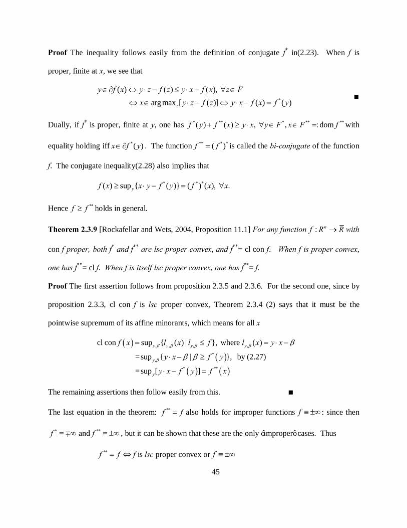
45
Proof The inequality follows easily from the definition of conjugate f* in(2.23). When f is
proper, finite at x, we see that
*
( ) ( ) ( ), arg max [ ( )] ( ) ( )z
y f x y z f z y x f x z Fx y z f z y x f x f y
∈∂ ⇔ ⋅ − ≤ ⋅ − ∀ ∈
⇔ ∈ ⋅ − ⇔ ⋅ − = ∎
Dually, if f* is proper, finite at y, one has * ** * ** **( ) ( ) , , : dom f y f x y x y F x F f+ ≥ ⋅ ∀ ∈ ∈ = with
equality holding iff *( )x f y∈∂ . The function ** * *( )f f= is called the bi-conjugate of the function
f. The conjugate inequality(2.28) also implies that
* * *( ) sup { ( )} ( ) ( ), .yf x x y f y f x x≥ ⋅ − = ∀
Hence ** f f≥ holds in general.
Theorem 2.3.9 [Rockafellar and Wets, 2004, Proposition 11.1] For any function : nf R R→ with
con f proper, both f* and f** are lsc proper convex, and f**= cl con f. When f is proper convex,
one has f**= cl f. When f is itself lsc proper convex, one has f**= f.
Proof The first assertion follows from proposition 2.3.5 and 2.3.6. For the second one, since by
proposition 2.3.3, cl con f is lsc proper convex, Theorem 2.3.4 (2) says that it must be the
pointwise supremum of its affine minorants, which means for all x
( )( )
( ) ( )
, , , ,
*,
* **
cl con sup { ( ) | }, where ( )
=sup { | }, by (2.27)
=sup [ ]
y y y y
y
y
f x l x l f l x y x
y x f y
y x f y f x
β β β β
β
β
β β
= ≤ = ⋅ −
⋅ − ≥
⋅ − =
The remaining assertions then follow easily from this. ∎
The last equation in the theorem: ** f f= also holds for improper functions f ≡ ±∞ : since then
* ** and f f≡ ∞ ≡ ±∞∓ , but it can be shown that these are the only ‘improper’ cases. Thus
** f f= ⇔ f is lsc proper convex or f ≡ ±∞

46
A function for which this equation holds is also called closed convex. For proper convex
functions closedness is equivalent to lower semi-continuity.
Theorem 2.3.10 [Rockafellar and Wets, 2004, Proposition 11.3] For any lsc proper convex
function f, one has
(2.29)
* 1 * 1
*
*
*
) ( ) and ( )b) ( ) ( )) ( ) argmax { ( )},
d) ( ) argmax { ( )}z
w
a f f f fy f x x f y
c f y y z f zf x x w f w
− −∂ = ∂ ∂ = ∂
∈ ∂ ⇔ ∈∂
∂ = ⋅ −
∂ = ⋅ −
For example, the function ( )geo x , being finite convex, is clearly lsc proper convex, has its
conjugate equal to the lsc proper convex function ( )ent δ , and the conjugate of which is then
( )geo x . The conjugate inequality relating this pair of functions is:
ln( ) ln ( ln( ) ln( / ))i i ix x xi i i i i ie x e eδ δ δ δ δ+ ≥ ⇔ ≥∑ ∑ ∑ ∑ ∑ ,
which is equivalent to the original geometric inequality (2.9), ( ) ii i iU U δδ≥∑ ∏ , (where
,ixiU e i= ∀ ). The condition for equality is ( ), . . / , , with i ix x
if i e e G i G eδ= ∇ = ∀ = ∑xδ .
The dual cone of any set S in nR is the closed convex cone
{ }: | 0, .nS y R y x x S+ = ∈ ⋅ ≥ ∀ ∈ When K itself is a closed convex cone, one has K K++ = .
Fenchel’s dual pair of conic programs
For any proper function f on Rn and any cone K in Rn, Fenchel’s conic program (P) and its dual
program (D) are respectively given by
(2.30) (P) inf{ ( ) | }p f x x F K= ∈ ∩ (D) * *inf{ ( ) | }d f y y F K += − ∈ ∩ ,

47
where p, d ∈[-∞, +∞], F and F* are the respective effective domains of f and f* (actually, F and
F* can both be omitted from the above formulation). If in addition, f and K are both closed
convex, the dual program of (D) is then (P); hence the formulation becomes completely
symmetric. The following result is immediate.
Lemma 2.3.11 (Main Lemma of Fenchel’s conic dual programs) Under the above setting
(2.30), one has * * ( ) ( ), , f x f y x F K y F K +≥ − ∀ ∈ ∀ ∈∩ ∩ ,
with equality holding if and only if ( )y f x∈∂ , and 0x y⋅ = , in which case x is optimal for
primal problem (P) and y is optimal for dual problem (D). Thus p ≥ d is always satisfied.
Theorem 2.3.12 (Fenchel’s Conic Duality Theorem) [Rockafellar, 1970, Theorem 31.4]
Assume that in the above setting(2.30), f and K are both convex.
a) If - , ri ( ) ri ( ) , p and F K then p d> ∞ ≠ ∅ =∩ , and d is attained.
b) If, furthermore, f and K are both closed, * , ri ( ) ri ( ) , d and F K then p d+< +∞ ≠ ∅ =∩ ,
and p is attained.
In general, x and y satisfy
* *( ) inf sup ( )K Kf x f f f y+= = − = −
if, and only if
( ), , , 0y f x x K y K x y+∈∂ ∈ ∈ ⋅ = .
The hypotheses ri ( ) ri ( )F K ≠ ∅∩ in (a) and * ri ( ) ri ( )F K + ≠ ∅∩ in (b) are commonly called
Fenchel’s hypothesis for the primal problem (P) and the dual problem (D), respectively. If either
of these conditions hold, and f and K are both closed, then p d= .

48
As an easy consequence of this, one has the following corollary:
Corollary 2.3.13 (Fenchel-Rockafellar’s Duality Theorem) [Rockafellar, 1970, Corollary
31.2.1] For any functions 1 2 : , :n mf R R f R R→ → , and a linear map : n mA R R→ , let ,p d R∈
be optimal values defined by the pair of programs below:
1 2inf [ ( ) ( )]nx Rp f x f Ax
∈= +
* *1 2inf [ ( ) ( )]m
Ty Rd f A y f y∈
= − − + .
These values satisfy p d≥ . If, furthermore, f1 and f2 are proper convex and satisfy the condition
(2.31) 1 2ri ( ) . . ri ( )x F s t Ax F∃ ∈ ∈ , (Fenchel’s hypothesis)
and - , p then p d> ∞ = , and d is attained.
This hypothesis is equivalent to the condition 11 2 ri ( ) ri ( )F A F− ≠ ∅∩ , which implies that
1
1 2 1 2ri ( ) , where dom , :F F F A F f f f f A−≠ ∅ = ∩ = = + o .
A special case of this result is obtained, when n m= and A is the identity map.
Corollary 2.3.14 (Fenchel’s Duality Theorem) [Rockafellar, 1970, Theorem 31.1] For any
functions 1 2 , : nf f R R→ , let ,p d R∈ be optimal values defined by the pair of programs below:
1 2inf [ ( ) ( )]nx Rp f x f x
∈= +
* *1 2inf [ ( ) ( )]ny Rd f y f y
∈= − − + .
These values satisfy p d≥ . If, furthermore, f1 and f2 are proper convex and satisfy the condition
(2.32) 1 2ri ( ) ri ( )x F F∃ ∈ ∩ ,
and - , then p p d> ∞ = and d is attained.
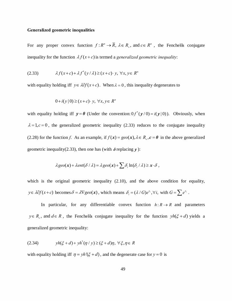
49
Generalized geometric inequalities
For any proper convex function : , , and n nf R R R c Rλ +→ ∈ ∈ , the Fenchel’s conjugate
inequality for the function ( )f x cλ + is termed a generalized geometric inequality:
(2.33) *( ) ( / ) ( ) , , nf x c f y x c y x y Rλ λ λ+ + ≥ + ⋅ ∀ ∈
with equality holding iff ( )y f x cλ∈ ∂ + . When 0λ = , this inequality degenerates to
0 ( | 0) ( ) , , ni y x c y x y R+ ≥ + ⋅ ∀ ∈
with equality holding iff =y 0 (Under the convention: *0 ( / 0) ( | 0)f i=y y ). Obviously, when
1, 0cλ = = , the generalized geometric inequality (2.33) reduces to the conjugate inequality
(2.28) for the function f. As an example, if ( ) ( ), ,f geo Rλ += ∈ =x x c 0 in the above generalized
geometric inequality(2.33), then one has (with δ replacing y ):
( ) ( / ) ( ) ln( / )i igeo ent geoλ λ λ λ δ δ λ+ = + ≥ ⋅∑x x xδ δ ,
which is the original geometric inequality (2.10), and the above condition for equality,
( )y f x cλ∈ ∂ + becomes ( )geoλ= ∇ xδ , which means ( / ) , , with i ix xi G e i G eδ λ= ∀ = ∑ .
In particular, for any differentiable convex function :h R R→ and parameters
, and y R d R+∈ ∈ , the Fenchel’s conjugate inequality for the function ( )yh dξ + yields a
generalized geometric inequality:
(2.34) *( ) ( / ) ( ) , ,yh d yh y d Rξ η ξ η ξ η+ + ≥ + ∀ ∈
with equality holding iff '( )yh dη ξ= + , and the degenerate case for 0y = is

50
0 ( | 0) ( ) , ,i d Rη ξ η ξ η+ ≥ + ∀ ∈
with equality holding iff 0η = (Under the convention: *0 ( / 0) ( | 0)h iη η= ).
2.4 KKT THEOREM FOR CONVEX PROGRAMS
In order to derive the first duality theorems for GP and for its extensions, we need to
apply the Karush-Kuhn-Tucker (KKT) theorem to the convex formulations of the various
extensions of GP. Let us consider in this section an (inequality-constrained) ordinary convex
program (CP)
(2.35) (CP) inf { ( ) | ( ) 0}F f∈ ≤x x g x
where 1( ) [ ( )]mi ig ==g x x , the functions 1 2, , ,..., : n
mf g g g R R→ are proper convex and satisfy
dom dom ,i iF f g G i= ⊂ = ∀ , { }| ( ) 0S F= ∈ ≤x g x is its feasible set. The perturbation
function : mv R R→ of (CP) is convex, where
(2.36) ( ) : inf { ( ) | ( ) }, .mFv f R∈= ≤ ∀ ∈xb x g x b b
This function is an antitone ( ) ( )v v≤ ⇒ ≥b u b u . Clearly, ( ) inf(CP) iff v S= < ∞ ≠ φ0 .
The function ( , ) : ( ) ( ) : ( , ]n mL x f x g x R Rλ λ += + ⋅ × → −∞ +∞ is the Lagrangian function of (CP).
For each fixed mRλ +∈ , it is a proper convex function in x with domain F. A vector mRλ ∈ is a
Lagrange multiplier vector for a point x F∈ if
(1) 0, ( ) 0, ( ) 0g x g xλ λ≥ ≤ ⋅ = and
(2) arg min ( , )xx L x λ∈ , i.e. x minimizes the function ( , ) over nL Rλ⋅ .

51
If, in addition the convex functions 1 2, , ,..., mf g g g are actually differentiable at x , then condition
(2) is equivalent to the gradient equation:
(2)’1
( ) ( ) 0mi ii
f x g xλ=
∇ + ∇ =∑ .
A vector pair ( , ) with , 0x x Fλ λ∈ ≥ is a saddle-point of the Lagrangian L and the
corresponding value ( , )L x λ a saddle-value of L if ( , ) ( , ) ( , ), L x L x L xλ λ λ≤ ≤ ∀x∈F, ∀λ∈
.mR+
Clearly, ( , ) with , 0x x Fλ λ∈ ≥ is a saddle-point of L iff λ is a Lagrange multiplier vector for x .
Theorem 2.4.1 (Lagrangian sufficient condition) If, in a convex program (CP) (2.35), a point
x F∈ has a Lagrange multiplier vector, say,λ then x is an optimal solution to (CP).
Proof This vector x is clearly feasible, i.e. S∈x . Moreover,
, ( ) 0 ( ) 0
( ) ( ) ( ) ( , ) ( , ) ( )S x F x g x
f f g x L x L x fλλ λ λ
∈ ⇒ ∈ ≤ ⇒ ⋅ ≤
⇒ ≥ + ⋅ = ≥ =
x gx x x
Hence x is optimal for (CP). ∎
Note this result actually does not depend on convexity.
We can summarize the above relationships to establish the following characterizations.
Theorem 2.4.2 For a differentiable convex program (CP)(2.35) where all the problem functions
are differentiable, its Lagrangian L, a vector mRλ ∈ , and a point x F∈ , the following three
conditions are equivalent:
1) The vectorλ is a Lagrange multiplier vector for x
2) The vector pair ( , )x λ forms a saddle-point of L

52
3) The vector pair ( , )x λ satisfies the following Karush-Kuhn-Tucker (KKT) optimality
conditions for (CP):
(a) 0, ( ) 0, ( ) 0g x g xλ λ≥ ≤ ⋅ =
(b) 1
( ) ( ) 0mi ii
f x g xλ=
∇ + ∇ =∑ .
Proof Show the implications 1) 2) 3) 1)⇒ ⇒ ⇒ are true. ∎
We say the convex program (CP) (2.35) satisfies a regularity condition known as the
Slater constraint qualification (Slater CQ) if ˆ ˆ s.t. ( ) 0, 1, 2,...,ix F g x i m∃ ∈ < ∀ = . This condition
means that int dom v∈0 . The following theorem, a central result in the study of convex
programs, tells us when a Lagrange multiplier vector exists for a solution to a convex program.
Theorem 2.4.3 (A Lagrange multiplier theorem: Lagrangian necessary conditions). [Borwein
and Lewis, 2006, Theorem 3.2.8] Suppose that the convex program (CP) (2.35) satisfies Slater
CQ and has an optimal solution x . Then the set of all Lagrange multiplier vectors for x is a
non-empty compact convex subset of mR+ .
Proof Since ( ) ( )v f=0 x is finite and int dom v∈0 , the convex value function v is proper
(Proposition 2.3.3), and the set ( )v∂ 0 is a non-empty compact convex subset of mR (Proposition
2.3.4). Let λ be any vector in ( )v−∂ 0 . Then it must satisfy
(2.37) ( ) ( ) ( ) , mf v v R= ≤ + ⋅ ∀ ∈x 0 b λ b b .
Since ( ) ( ), mv v R+≤ ∀ ∈b 0 b , this, together with (2.37) implies that
( ) ( ) ( ) , 0 , m m mv v v R R R+ + +≤ + ⋅ ≤ + ⋅ ∀ ∈ ⇒ ≤ ⋅ ∀ ∈ ⇒ ∈0 b λ b 0 λ b b λ b b λ .
Note that ( ( )) ( ), v g f F≤ ∀ ∈x x x . This and (2.37) with ( ), g F= ∈b x x implies that

53
(2.38) ( ) ( ( )) ( ) ( ) ( ) ( , ), f v g g f g L F≤ + ⋅ ≤ + ⋅ = ∀ ∈x x λ x x λ x x λ x
In particular, when =x x , this implies that 0 ( ) ( ) 0g g≤ ⋅ ⇒ ⋅ =λ x λ x , as 0, ( ) 0g≥ ≤λ x .
It then follows from (2.38) that ( , ) ( ) ( , ), nL f L R= ≤ ∀ ∈x λ x x λ x , and we see that λ a Lagrange
multiplier vector for x . ∎
Theorem 2.4.4 (Karush-Kuhn-Tucker theorem) [Rockafellar, 1970, Corollary 28.3.1] For a
differentiable convex program (CP) (2.35) satisfying Slater CQ, its Lagrangian L, and a vector
nx R∈ , the following conditions are equivalent:
1) x is an optimal solution to (CP).
2) There exists a vector mRλ ∈ such that ( , )x λ forms a saddle-point of L.
3) There exists a vector mRλ ∈ such that ( , )x λ satisfies the KKT conditions for (CP):
(a) 0, ( ) 0, ( ) 0g x g xλ λ≥ ≤ ⋅ = (b) 1
( ) ( ) 0mi ii
f x g xλ=
∇ + ∇ =∑ .
2.5 THE EXISTENCE OF A PRIMAL MINIMAL SOLUTION
A function : nf R R→ is (lower) level-bounded if its level sets f α≤ are bounded α∀ ∈ R , i.e.
| | ( )x f x→ ∞ ⇒ → ∞ . Note that
(2.39) , R f f fα β β
β α β α
α ≤ < ≤
> >
∀ ∈ = =∩ ∩ .
In particular, if f is a proper function, inf fα = < ∞ then the minimum set, argmin f = f fα α= ≤=
is the intersection of a nonempty family of nested (i.e. '' f fβ ββ β ≤ ≤≤ ⇒ ⊂ ) non-empty level

54
sets f β≤ which are compact if f is also lsc and level-bounded. This minimum set must be non-
empty, according to Cantor’s intersection theorem in real analysis.
Theorem 2.5.1 (Attainment of a minimum) [Rockafellar and Wets, 2004, 1.9] Suppose
: nf R R→ is lsc, proper, and level-bounded. Then inf f is finite and the set argmin f is
nonempty and compact.
The functions we are going to deal with in CGP problems are finite-valued convex, hence
they are lsc proper convex, with closed convex level sets whose bounded-ness property are
equivalent to the lack of direction of recession. In nR space, a non-zero vector d is a direction of
recession of a non-empty set C if the ray set { }: | x R d x td t R+ ++ = + ∈ is contained in C for all x
in C. We define the (global) recession cone of C, CR to be the set { }| nd R C R d C+∈ + ⊂ and
the horizon cone of C, C∞ to be the unique set S with cl (0, ) (0, ), where : (1, )nK R S K R C+∩ = = .
Below we let {0,1,2,...}Z+ = and \{0} (0, )R R++ += = +∞ .
Theorem 2.5.2 For any non-empty set C in nR , the recession cone { | , 0}C xC tR x C t−= ∈ >∩ is a
convex cone, the horizon cone { }| , 0 with n i ii iC d R x C t t x d∞ += ∈ ∃ ∈ → → is a closed cone,
and they satisfy:
'1 , 0, ( ) , , (0, )=cl \ (1,cl )C C C CtR K C t R R x C x C C K R C∞ ∞ ∞++⊂ ⊂ ∀ > ⊂ ⊂ ∀ ∈
where
{ } { } { }
{ } { }' '
0
: ( ) | | | ,
( ) : | | ( ) ,
Cx C
C xC Ct
t
K C x d C d C d C Z d C d x Z d C x C
R x d x R d C d x Z d C and R x is a cone x C
+ +∈
−+ +
>
= − = + ⊂ = + ⊂ ⊂ + ⊂ ∀ ∈
= = + ⊂ ⊂ + ⊂ ∀ ∈
∩
∩
When C ≠ φ is a closed convex set, these sets coincide into a closed convex cone

55
(2.40) ' ( ), C C CR K C R x x C∞= = = ∀ ∈ .
If, furthermore, C∈0 then '
0( )C C CR K C R C
λλ∞
>= = = =0 ∩ .
Note that ' 1
0( )C C Ct
x C tR R x K
∈ >= =∩ ∩ and that{ }| ,d x Z d C C x C∞
++ ⊂ ⊂ ∀ ∈
Corollary 2.5.3 For any family of closed convex sets { | }iC i I∈ with non-empty intersection,
: ii I
C C∈
= ≠ ∅∩ one has ii I
C C∞ ∞
∈= ∩ .
Theorem 2.5.4 In nR space, a set C is bounded iff { } :C∞ = =0 O , a closed convex set C ≠ φ is
bounded iff { } | C d x R d C x C∞+= + ⊂ = ∀ ∈O, , i.e. no and with d x C x R d C+∃ ≠ ∈ + ⊂0 .
Definition 2.5.5 For any lsc proper convex function f its recession (or horizon) function f ∞ is
given by
(2.41) [ ] [ ]1 1
0( ) : sup ( ) ( ) lim ( ) ( ) , if t ttt
f d f x td f x f x td f x x F∞
→∞>= + − = + − ∈
In particular,
(2.42) 10
( ) lim ( ) lim ( / ), if 0ttf d f td f d F
λλ λ∞
→∞ ↓= = ∈
Moreover, if f is also ph, f f∞ = , e.g. for any nonempty convex set C, the function SC is lsc
proper sublinear, hence C CS S∞ = . If f has bounded domain F, then for any nonzero d, the ray set
x td+ for large t will eventually leave F , hence 0f i∞ = , e.g. since the entropy function
( )*ent geo= has bounded domain { }: | 1 n Tn R+∆ = ∈ =y 1 y (the unit simplex), 0ent i∞ =
Proposition 2.5.6 (A simple rule) Let : nf R R→ be an lsc proper convex function,
: , , :n mA n m b R g R R× ∈ → be defined by ( ) : ( )g z f Az b= + with domain 1: ( )G A F b−= − ≠ φ .

56
Then g is also lsc proper convex with its recession function given by
( ) ( ) [( ) ]g d f Ad f Ad b∞ ∞ ∞ ∞= = + , where 1 1( ) [( ) ] [ ]i n ni i
∞ ∞= == = =i iAd + b a d + b a d Ad .
Proof g is clearly proper convex, it is also lsc [Rockafellar and Wets, 2004, 1.40 (a)]. If z G∈ ,
then Az b F+ ∈ and
[ ] [ ]1 1( ) lim ( ) ( ) lim ( ) ( ) ( )t tt tg d g z td g z f Az b tAd f Az b f Ad∞ ∞
→∞ →∞= + − = + + − + = ∎
Our knowledge about horizon function can help us calculate the horizon cone of level sets and
epigraph of an lsc proper convex function.
Theorem 2.5.7 Let : nf R R→ be any lsc proper convex function, then
(2.43) 0( ) ( ) ( ) ( ) (epi ) epi a f f b f fα≤ ∞ ∞ ≤ ∞ ∞= = .
Hence the minimum set argmin f is non-empty and bounded iff 0 ( ) 0no d such that f d∞∃ ≠ ≤ ,
and the recession function f ∞ is lsc proper sublinear.
Proof (a) ( , )α α∀ ∈ +∞ , where inf fα = < ∞ , the level sets f α≤ are non-empty closed convex,
hence by (2.40) one has
10
( ) , 0, if ( ) , 0, if ( ) ( ) ( ), 0, if ( ) sup [ ( ) ( )] 0, if t t
d f x td f t x ff x td t f xf x td f x t x Ff d f x td f x x F
α α α
α α
≤ ∞ ≤ ≤
∞>
∈ ⇔ + ∈ ∀ > ∈⇔ + ≤ ∀ > ≤⇔ + ≤ ∀ > ∈
⇔ = + − ≤ ∈
So 0( ) ( ) , ( , )f fα α α≤ ∞ ∞ ≤= ∀ ∈ +∞
(b) Since f is lsc proper convex, epi f is non-empty closed convex, hence by (2.40) one has
( , ) (epi ) ( , ) epi , 0, if ( , ) epi ( ) , 0, if ( ) ( ) ( ), 0, if ( ) s
d f x td t f t x ff x td t t f xf x td t f x t x Ff d
µ α µ αµ α αµ
∞
∞
∈ ⇔ + + ∈ ∀ > ∈⇔ + − ≤ ∀ > ≤⇔ + − ≤ ∀ > ∈
⇔ = 10up [ ( ) ( )] , if t t f x td f x x Fµ> + − ≤ ∈

57
So (epi ) epi f f∞ ∞= is a closed convex cone, f ∞ is lsc proper sublinear, and the rest
are obvious. ∎
In the above theorem, the closed convex cone 0( )f ∞ ≤ is called the recession cone of f,
whose nonzero vectors are called directions of recession of f. The following is an important
duality result. For example, for the function 2( ) 1f x x= + , since 0 F∈ ,
2 21 ( ) lim 1 | |ttf d t d d∞
→∞= + = , the recession cone of f is 0| |d ≤ = O , so f is level-bounded and its
minimum set is non-empty and bounded, namely {0}. Indeed, we have the level sets
2 21, 1 all nonempty and bounded, 1f α α α α≤ = − − + − ∀ ≥
, and 1arg min {0}f f ≤= = .
Theorem 2.5.8 (horizon functions as support functions) [Rockafellar, 1970, Theorem 13.3] Let
: nf R R→ be a proper convex function, then
1) *Ff S∞ = , and * 0( ) ( )f F∞ ≤ −= (recession cone of f* = polar cone of F)
2) if f is also lsc, then *Ff S∞ = , and 0 *( ) ( )f F∞ ≤ −= (recession cone of f = polar cone of F*)
Proof (1) By (2.23) we have *,( , ) epi
epi epi xx ff l αα ∈
= ≠ ∅∩ , since *f is proper. Then by
Corollary 2.5.3 we have: *,( , ) epi
(epi ) (epi )xx ff l αα
∞ ∞
∈= ∩
and then by (2.43) (b), *, ,0( , ) epi ( , ) epi
epi epi epi x xx f x ff l lαα α
∞ ∞
∈ ∈= =∩ ∩
which means *, ( ) sup{ | ( , ) epi } sup{ | } ( )Fd f d x d x f x d x F S dα∞∀ = ⋅ ∈ = ⋅ ∈ = ,
Hence we have *Ff S∞ = , and { }* 0 0( ) ( ) | sup 0n
F x Ff S y R y x F∞ ≤ ≤ −∈= = ∈ ⋅ ≤ =
(2) If f is also lsc, then apply (1) to f* and the result follows. ∎

58
For instance, if f is the affine function on nR , , ( )al x a xβ β= ⋅ − , then
** * *
0( ) ( ) , ( ) ( ), { }, ( ) ( ) ( ), na FF
f y i y f d a d S d F a f d i d S d F Rβ ∞ ∞= + = ⋅ = = = = = .
Since the geometric function geo has domain *0, n
FF R ent geo S i∞ ∞= = = = .
Corollary 2.5.9 Let C be a nonempty convex set, then
1) 0, C C CS S S C∞ ≤ −= = , (recession cone of CS = polar cone of C)
2) if C is also closed, then ( )CC B∞ −= , (recession cone of C = polar cone of barrier cone
of C)
Proof Apply this theorem to the function Cf i= . ∎
Theorem 2.5.10 (dual properties of minimization) [Rockafellar, 1970, Theorem 27.1] Let
: nf R R→ be any lsc proper convex function. Then
a) *inf (0)f f= − . Thus f is bounded below iff *0 F∈
b) argmin f *(0)f= ∂ . Thus inf f is attained iff * 0 dom f∈ ∂ . This is implied by *0 ri F∈ .
c) argmin f is non-empty and bounded iff *0 int F∈ iff f has no directions of recession.
d) argmin f { }x= iff *f is differentiable at 0 and
*(0)f x∇ = .
The problem setting
We now consider an inequality-constrained convex program (CP) where the index set
ˆ{1, , }, : {0}K p K K= = ∪L , each function ˆ, kf k K∀ ∈ is an lsc proper convex function,
(2.44) (CP) 0 0inf { ( ) | , ( ) 0, } : infn kx Rf x x F f x k K f
∈∈ ≤ ∀ ∈ =
where 0 Sf f i= + is the objective function of this program (CP), 0 0dom F f= , and the feasible set
is { }0 ( ) 0, kS F f k K= ∈ ≤ ∀ ∈x x . We assume that S ≠ ∅ so that for α sufficiently large, the

59
level set of f, 0 00 1 pf f f fα α≤ ≤ ≤ ≤= ∩ ∩ ∩L is non-empty and closed convex, and the function f is
also lsc proper convex. The direction of recession of the objective function f shall be called the
direction of recession of the program (CP), which as the following theorem shows, is the
direction of recession common to all the problem functions in (CP).
Theorem 2.5.11 In the above consistent convex program (CP)(2.44), the recession cone of its
objective function f is
(2.45) { }0 ˆ( ) | ( ) 0, nkf d R f d k K∞ ≤ ∞= ∈ ≤ ∀ ∈ .
Hence the direction of recession of the objective function f is the direction of recession common
to all the problem functions fk in (CP), and the minimum set of the program (CP) is non-empty
and bounded iff the system ˆ( ) 0, kf d k K∞ ≤ ∈ has no non-trivial solution in d, which means that
program (CP) has no directions of recession.
Proof Since for α sufficiently large, the recession cone of f is
0 0 00 1
0 00 1
0 0 00 1
( ) ( ) ( ) , by (2.45) (a)
=( ) ( ) ( ) , by Corollary 2.5.3
=( ) ( ) ( ) , by (2.45) (a)
p
p
p
f f f f f
f f f
f f f
α α
α
∞ ≤ ≤ ∞ ≤ ≤ ≤ ∞
≤ ∞ ≤ ∞ ≤ ∞
∞ ≤ ∞ ≤ ∞ ≤
= = ∩ ∩ ∩
∩ ∩ ∩
∩ ∩ ∩
L
L
L
{ }ˆ = | ( ) 0, nkd R f d k K∞∈ ≤ ∀ ∈
Hence the direction of recession of the objective function f is the direction of recession common
to all the problem functions fk in (CP). The minimum set of program (CP) is non-empty and
bounded ⟺ f is level-bounded ⟺ the recession cone of f is a zero cone
⟺ the system ˆ( ) 0, kf d k K∞ ≤ ∈ has no non-trivial solution in d
⟺ there are no direction of recession common to all problem functions of (CP).
⟺ Program (CP) has no direction of recession. ∎

60
3.0 ALTERNATIVE PROOFS AND SOME REFINEMENTS OF THE DUALITY
THEOREMS OF GP
Since the method we are going to use to derive the basic duality theories for the exponential,
quadratic, lp, and composite (posynomial) GP are significantly different from existing methods in
the literature used for posynomial GP, it seems appropriate to test our method on posynomial GP
first to confirm its validity, and also to familiarize the readers with this new approach for the
subsequent rather complicated extended GP models in the later chapters. Equation Chapter 3 Section 1
CONVEXITY PROPERTY OF 1
( ) : ln[ exp ] :n nii
geo x R R=
= →∑x
First note that geo(x) is a finite-valued function with inf geo(x) =− ∞ and sup geo(x) =+∞.
Fact 3.1 (A variant of Holder’s inequality) [Hardy, et.al. 1952, pp.21-22] Given positive weights
0, 0, 1,α β α β> > + = and two sets of non-negative numbers U 0, V 0,i i≥ ≥ one has
(3.1) 1 1 1U ( U ) ( )n n n
i i i ii i iV Vα β α β
= = =≤∑ ∑ ∑
where ‘=’ holds exactly when1 1
( ) ( U ), ,n ni i i ii i
U V V i= =
= ∀∑ ∑ namely, the sum of the geometric
means is not greater than the geometric mean of the sums, with’=’ holding if and only if the two
sets of numbers are in proportion.
Proof When one of the sums1 1
: U or :n ni ii i
U V V= =
= =∑ ∑ equals zero, the inequality trivially
holds as an identity: 0=0. Otherwise, we can divide both sides by U Vα β and show that

61
1 1
1n n
i i i i
i i
U V U VU V U V
α β
α β α β= =
≤ + = + = ∑ ∑ ,
by AGM inequality, then (3.1) follows. Clearly, equality holds iff Ui/U=Vi /V, for all i, which
means, UiV=Vi U, for all i. ∎
The convexity of geometric functions geo(x) is an easy consequence of the above inequality.
Fact 3.2 The geometric function 1
( ) : ln[ exp ]nn ii
geo x x=
= ∑ is convex on nR , specifically
(3.2) ( ) ( ) ( ), , , 0, 0, 1,nn n ngeo x y geo x geo y x y Rα β α β α β α β+ ≤ + ∀ ∈ ∀ > > + =
with equality holding iff , 1, where 1=(1, ,1)t nt R y x t R∃ ∈ = + ∈L . (So it is not strictly convex)
Proof Setting , ,i ix yi iU e V e i= = ∀ in (3.1) yields
( ) ( )1 1 1 1( ) ( ) ( )i i i i i i
n n n nx y x y x yi i i i
e e e e eα β
α βα β += = = =
= ≤∑ ∑ ∑ ∑ .
Take logarithms of both sides of the above, (3.2) follows. Moreover, equality holds iff the two
sets of numbers and i ix ye e are in proportion: 0, , ,i iy xT e Te i∃ > = ∀ or equivalently,
( ln ), 1, where 1=(1, ,1)t nt T y x t R∃ = = + ∈L . ∎
Fact 3.3 (Faithful convexity of the function geo) [Rockafellar, 1970b] If geo(x) is affine on any
line segment L { }[ , ] : ( ) | [0,1]x y x r y x r= + − ∈ joining two points x and y, it is affine on the line
extending that segment: { }( , ) : ( ) |L x y x r y x r R= + − ∈ .
Proof If geo(x) is affine on [x, y], then by this proposition, (3.2) must hold as equality and y
=x+t1, for some real t. We readily see that along the line { }( , ) : ( 1) |L x y x r t r R= + ∈ , geo(x) is
affine with slope t:
(3.3) ( ( 1)) ( ) , ,geo x r t geo x rt r t R+ = + ∀ ∈ ∎

62
This proposition says: The function geo(x) is affine along any line in the direction of the sum
vector 1= (1,…, 1)T, yet it is strictly convex along lines in any other direction. Thus the function
geo(x) has linearity 1 and rank n-1 [Rockafellar 1970, p.70]. It is also strictly isotone: any
points 1 2x x≤ in Rn satisfy 1 2 ( ) ( )geo x geo x≤ with equality holding iff 1 2 x x= .
3.1 MAIN LEMMA OF GP
The GGP formulation of (GP) in the variables =: ix i I∈ia z, is
(3.4) (GP)x 0 0 inf ( ) . . ( ) 0, , n
k kR
geo s t geo k K∈
+ + ≤ ∀ ∈ ∈x
x c x c x P ,
where ia is the ith row of the exponent matrix A, { } | mR= ∈Az zP is the column space of A, kx is
the sub-vector of x obtained by deleting all of its components xi for which i is not in [k], and
{ }[ ]( ) ln exp( )k k
i ii kgeo x c
∈+ = +∑x c is convex by Fact 3.2. Of course, we have
ˆ( ) ( ) ln ( ),k kk kgeo g G k K+ = = ∀ ∈x c z t . The associated dual program (GD) is given below with
each dual variable iδ corresponding to a primal term iU .
Dual posynomial program (GD) under the convention that 00=1.

63
(3.5) (GD)
( )
( )
ˆ [ ]
1 1
0
1
[ ]
sup ( ) :
. . 1,
0,
ˆwhere : , .
i
n
i k
i k ik K i kR
pn
i i ki k
n
ij ii
k ii k
V C
C
s t
a j J
k K
δ
δ λ
λ δ
δ λ
λ
δ
λ δ
+∈ ∈
∈
= =
=
∈
= = ⋅
= = ∈
= ∈
∏ ∏
∏ ∏
∑
∑
δδ
We now provide an alternative proof for the main lemma of (GP) (cf proof of Lemma 2.0).
Lemma 3.1.0 (Main Lemma of GP) If t is feasible for primal program (GP) and δ is feasible
for dual program (GD), then
0 ( ) ( ).G V≥t δ
Moreover, under the same conditions 0 ( ) ( ),G V=t δ if, and only if, one of the following two sets
of equivalent conditions holds:
(3.6) { }
( ) 1, , (a)( ) ( ), [ ] (b), 0
kk
i k k i
G k KG U i k k K
λ
δ λ
= ∀ ∈
= ∀ ∈ ∀ ∈ ∪
tt t
(Extremality condition 1)
(3.7) 0( ) ( ) , [0] (c)( ), [ ], (d),
ii
k i
U G iU i k k K
δλ
∈= ∈ ∀ ∈
t tt
(Extremality condition 2)
in which case t is optimal for primal program (GP) and δ is optimal for dual program (GD).
(Recall from Lemma 2.1.0 that the above two sets of extremality conditions are equivalent.)
Proof: Assume that t is feasible for primal program (GP) and δ for dual program (GD), then the
transformed variables , with = , = ln , , i j jA x z t j J i I= ∈ ∈ix z a z are feasible for (GP)x, thus we
have ( ) 0, , and 0, k kkgeo k K k Kλ+ ≤ ∀ ∈ ∈ ≥ ∀ ∈x c x P, , so that by (2.3), 0⋅ =x δ and
(3.8) 0 0 0 01
( ) ( ) ( )p k kkk
geo geo geoλ=
+ ≥ + + +∑x c x c x c .

64
Applying the generalized geometric inequality (2.33) to each function ˆ( ), ,k kk geo k Kλ + ∈x c
with λ0=1 yields
(3.9) ( )
( )[ ] [ ]
[ ] [ ]
( ) ln / ( )
ˆ = ln / ,
k kk i i k i i ii k i k
i i k i i ii k i k
geo x c
C x k K
λ δ δ λ δ
δ λ δ δ∈ ∈
∈ ∈
+ ≥ − + +
+ ∀ ∈
∑ ∑∑ ∑
x c
where equality holds iff ( )k k kk geoλ= ∇ +x cδ , i.e., ( ( ) / ( )), [ ].i k i kU G i kδ λ= ∀ ∈t t
Summing over all these inequalities yields
(3.10) ( )
( )0 0 [ ] 0 [ ]
0 [ ]
( ) ln /
= ln / ln ( ), 0
p p pk kk i i k i i ik k i k k i k
pi i k ik i k
geo C x
C V
λ δ λ δ δ
δ λ δ
= = ∈ = ∈
= ∈
+ ≥ +
= ⋅ =
∑ ∑ ∑ ∑ ∑∑ ∑
x c
x δ∵δ.
Combining inequalities (3.8) and (3.10) shows
(3.11) ( )0 00 0 [ ]
( ) ( ) ln / ln ( )p pk kk i i k ik k i k
geo geo C Vλ δ λ δ= = ∈
+ ≥ + ≥ =∑ ∑ ∑x c x c δ
Hence 0 0( ) ln ( )geo V+ ≥x c δ with equality holding iff the two inequalities (3.8) and (3.9) both
hold as equalities, which means complementary slackness conditions ( ) 0,k kk geo k Kλ + = ∀ ∈x c
as well as the gradient (or proportionality) conditions ˆ( ) ( ), [ ], i k k iG U i k k Kδ λ= ∀ ∈ ∀ ∈t t must
hold true. Exponentiating the far two sides of inequality (3.11) and the above complementary
slackness conditions, one obtains 0 ( ) ( )G V≥t δ with equality holding iff the Extremality
condition 1 hold true. ∎
In (3.10), the function on the left is the Lagrangian of the primal program (GP)x
given by 0 01
( ) ( )p k kkk
geo geoλ=
+ + +∑x c x c , and the negative of its conjugate is the last
expression, namely ( )0 [ ]ln / ln ( )p
i i k ik i kC Vδ λ δ
= ∈=∑ ∑ δ . Thus the dual objective ( )V δ of (GD)
is the exponential of the negative of the conjugate of the Lagrangian of the primal program

65
(GP)x. We have actually proved the main lemma of (GP) by the conjugate inequality for the
Lagrangian of (GP)x and its conjugate. We shall see that this same principle also works for
(CGP).
It follows from this lemma that we always have ( ) ( ) inf GP sup GD 0∞ ≥ ≥ ≥ . If (GP)
and (GD) are both feasible, and inf (GP) = sup (GD), we say there is no duality gap between
these two programs. One way to show this is to prove that 0, , , s.t. Tε∀ > ∃ ∈ ∈ ∆t δ
0 ( ) ( ) ,G V ε− ≤t δ where T and ∆ are the feasible sets for the programs (GP) and (GD),
respectively. If, in addition, the two optimum values are both attained, i.e. min (GP) = max (GD),
we say perfect duality holds. In this case, if an optimum solution for one program can be easily
converted to an optimum solution for the other program, then the two programs (GP) and (GD)
may be deemed equivalent in this sense. The duality theory for GP attempts to find the
conditions under which the above desirable outcomes would result, so that it is possible to solve
the primal through its dual. This is referred to as a GP dual approach.
EXAMPLE 3.1.1 (Maximum Likelihood Estimator of a Bernoulli Parameter) [Ross, 2004,
p.231] Suppose that n independent trials, each of which is a success with probability p, are
performed. What is the maximum likelihood estimator of p?
Solution The likelihood function to be maximized is
1, 1( , | ) (1 ) , with , 0 or 1,nk n k
n i iif x x p p p k x x i−
== − = = ∀∑L
This can be formulated as a three-term, two-variable (n=3, m=2) GP example:
1
( , ) 0inf s.t. 1k k n
p qf p q p q− − −
>= + ≤

66
* *1
1
2
3
The exponent matrix and a unique dual solution is =
1 1 0
0 1
p q nk k n
kn k
δ λδδδ
− − −
,
From extremality condition 2, i.e., (3.7) (d), we see that
*
*2 1*1
ˆ, so n
iXk p pn n
δλ
= = = ∑ . ∎
The following corollary is immediate from the main lemma of GP.
Weak Duality Theorem of GP
i) Always, ( ) ( ) inf GP sup GD 0.∞ ≥ ≥ ≥
ii) When (GP) is feasible, ( ) ( )inf GP sup GD .∞ > ≥
i.e. if sup(GD)=∞ , (GP) is infeasible.
iii) When (GD) is feasible, ( ) ( )inf GP sup GD 0.≥ >
i.e. if inf (GP)=0 , (GD) is infeasible.
iv) When (GP) and (GD) are both feasible, ( ) ( ) inf GP sup GD 0.∞ > ≥ >
3.2 FIRST DUALITY THEOREM OF GP
In this section we shall work with the (GP)z formulation in the variables := ln , j jz t j J∈
(GP)z
0inf ( ) . . ( ) 0, m kR
g s t g k K∈
≤ ∀ ∈z
z z

67
where 1( , , )mz z=z L and { }[ ]( ) : ln ( ) ln exp[ ] = ( )i k k
k k ii kg G c geo
∈= = + +∑z t a z A z c is convex by
Proposition 2.3.1 and Fact 3.2. The Lagrangian for this differentiable convex program (GP)z is
0( , ) : ( ) ( ), , .p mk kk K
l g g R Rλ +∈= + ∀ ∈ ∈∑z z z zλ λ
Theorem 3.2.1 (cf Theorem 2.1.1) (First Duality Theorem of GP) Suppose that primal
program (GP) is superconsistent. Then the following 3 conditions are equivalent:
1) t’ is a minimal solution to (GP).
2) There exists a vector ' pR+∈λ for z′ (where z′= ln t′) such that ( ', ')z λ forms a saddle
point of ( , )l z λ .
3) There exists a vector ' pR+∈λ for z’ (where z’= ln t’) such that ( ', ')z λ satisfies the KKT
conditions for (GP)z:
' '
' '0ˆ
( ) 0, ( ) 0, ( ) 0,
( ) ( , ') ( ) , 1k k k k
z k kk K
a g g k K
b l g where
λ λ
λ λ∈
≥ ≤ = ∀ ∈
∇ = ∇ = =∑z' z'
z' z' 0λ
in which case the set of all such vectors 'λ is a non-empty compact convex subset of pR+ ,
and the dual program (GD) also has a maximum solution 'δ such that
0min(GP) ( ') ( ') max(GD)G V= = =t δ (Perfect duality)
Moreover, each pair of primal and dual optimal solution ( )t',δ' satisfies
(3.12) ' '
' ' '
( ), [0]( )
, [ ], , and 0i
ii k k
V iU
i k k K
δ
δ λ λ
∈= ∈ ∈ >
t'δ
Proof: By assumption, the differentiable convex program (GP)z satisfies the Slater CQ. Hence
by KKT Theorem (Theorem 2.4.4), the above conditions 1) through 3) are equivalent and

68
therefore, by Theorem 2.4.3 the set of all such vectors 'λ is a non-empty compact convex subset
of pR+ , and conditions (a) and (b) in 3) hold. We note that
Condition (b)'
'
ˆ ˆ [ ]
( ) 0, ( ) 0, ( )
k kk ij i
i kk K k Kj k
g j J a U j Jz G
λλ∈∈ ∈
∂⇒ = ∀ ∈ ⇒ = ∀ ∈
∂∑ ∑ ∑z' t't'
, by (1.8)
If we define ' ' ˆ( ) / ( ) 0, [ ],i k i kU G i k k Kδ λ= ≥ ∀ ∈ ∀ ∈t' t' in the above, we have the orthogonality
condition in (GD): ' '
ˆ [ ]0, .ij i ij i
i k i Ik K
a a j Jδ δ∈ ∈∈
= = ∀ ∈∑ ∑ ∑
Condition (a)'
( ) 1, kkG k Kλ⇒ = ∀ ∈t' , this is condition (a) in the extremality condition 1 (3.6) for
main lemma of (GP), and the condition (b) in (3.6) is clearly true by our definition of 'δ . Lastly,
we see that ' ' '
[ ] [ ]
ˆ[ ( ) / ( )] , i k i k ki k i k
U G k Kδ λ λ∈ ∈
= = ∀ ∈∑ ∑ t' t' . We have thus defined a dual feasible
solution δ′ which, together with the minimal solution t′, satisfies the extremality condition 1 in
(3.6). Hence by main lemma of (GP), this δ′ is a maximal solution satisfying
0min(GP) ( ') ( ') max(GD)G V= = =t δ
Since (3.6) and (3.7) are equivalent, and the latter condition implies(3.12). ∎
Obviously, our Theorem 3.1 has a stronger conclusion than that of Theorem 2.1.
3.3 SECOND DUALITY THEOREM OF GP
To prove the second duality theorem of (GP) we will apply Theorem 2.5.10 to (GP)z which fits
into the problem setting (2.44), because all of the problem functions ( )kg =z
{ }[ ]ln exp[ ] = ( )i k k
ii kc geo
∈+ +∑ a z A z c are finite convex on Rm. Hence they are lsc proper

69
convex. Thus we need to compute the recession functions kg∞ for all of the problem functions gk,
and that leads us to the computation of geo∞ , as ( ) ( )kkg geo∞ ∞=d A d by Proposition 2.5.6 and by
the fact that ( )= ( )k kkg geo +z A z c .
Recession function of geo (x)
Since geo(x) is finite-valued convex with 0 in the domain, it is lsc proper convex and we
can apply (2.42) to compute its recession function:
(3.13) ( )0
1lim ( / ) lim ( )t
geo geo geo ttλ
λ λ∞
↓ ↑∞= =d d d
We define the max function max : nR R→ by maxn(x) =: 1maxni ix= for 1( , , ) n
nx x x R= ∈L (The
subscript n can usually be omitted). This function is clearly finite sublinear, hence it is lsc and
proper. It is also an isotone: any points 1 2x x≤ in Rn satisfy max(x1) ≤ max(x2), and is not strictly
convex (since max (tx) =t max (x), for all t≥ 0).
Fact 3.4 (recession function of geometric function geo) The non-smooth function maxn (x) can be
approximated uniformly, to any accuracy, by a smooth function (�⋆geon) (x) = :λgeon (x/λ):
(3.14) ( )0 sup [ geo / max ( )] ln , 0x n nx x nλ λ λ λ≤ − ≤ ∀ > .
(3.15) ( )geo max( ),x x x∞ = ∀
Proof Let maxn(x) =xk. Then 1
k i knx x xe e ne≤ ≤∑ and thus ( ) lnk n kx geo x x n≤ ≤ + , which implies
(3.16) 0 ( ) max ( ) ln , n ngeo x x n x≤ − ≤ ∀
Homogenize this and we get(3.14). Let λ↓0in(3.14), then ( )/ max ( ),n ngeo x xλ λ → uniformly,
so (3.15) follows by(3.13). ∎

70
An alternative proof of (3.15)
Since *geo ent= with domain *nF = ∆ (the unit simplex), one has by Theorem 2.5.8
{ }{ }
( ) ( ) sup | 1, , a knapsack problem
= inf | , 1, , , by LP duality theory max( )
n
T n
i
geo S R
d i nλ λ
∞∆ += = ⋅ = ∈
≥ ∀ =
=
d d d y 1 y y
dL ∎
Since ( )= ( )k kkg geo +z A z c , by Proposition 2.5.6 we have ( ) ( ) max( )k k
kg geo∞ ∞= =d A d A d .
A theorem of the alternatives from linear programming duality theory
Of the following two linear systems exactly one has a solution (where A is an n by m matrix):
(I) Find z with 0 0A≠ ≤z (II) Find y with 0, 0TA> =y y
Recall that program (GD) is canonical if system (II) has a solution with A being its exponent
matrix.
Theorem 3.3.1 (cf Theorem 2.1.2) (Second Duality Theorem of GP) Suppose that primal
program (GP) is consistent. Then the minimum set of program (GP)z is non-empty and bounded
iff dual program (GD) is canonical, in which case program (GP) has a minimum solution t’.
Obviously, this theorem is stronger than the original second duality theorem of GP (Theorem
2.2), and it also includes its converse.
Proof By assumption, program (GP)z is also consistent. Now
ˆ ˆ( ) 0, max( ) 0, ˆ ,
ˆ 0, [ ], 0,
kk
k
g k K k K
k K
i k k Ki I
∞ ≤ ∈ ⇔ ≤ ∈
⇔ ≤ ∈
⇔ ≤ ∈ ∈
⇔ ≤ ∈ ⇔ ≤
i
i
d A d
A d 0
a da d Ad 0
Since A is of full column rank, it is one-to-one, hence 0 0≠ ⇒ ≠d Ad . Therefore by Theorem
2.5.10, one has

71
The minimum set of program (GP)z is non-empty and bounded
⇔ The system ˆ( ) 0, kg d k K∞ ≤ ∈ has no non-trivial solution in d
no with 0 0d Ad⇔ ∃ ≠ ≤ , i.e. system (I) above has no solution
⇔ System (II) above has a solution
⇔ Program (GD) is canonical
In this case, program (GP) must have a minimum solution t’. ∎
The original second duality theorem (Theorem 2.2) has been refined by the original authors:
Theorem 3.3.2 (Strong Duality Theorem of GP) [Duffin et.al 1967, p.173, Theorem 1(ii)]
If dual program (GD) is canonical and has a finite positive supremum, then primal program
(GP) has a minimum solution 't closing the duality gap:
0 ( ) min( ) sup( )G GP GD= =t'
Compared to Theorem 2.2, the assumption of this theorem is weaker, since by the weak duality
theorem of GP (iv) the condition that primal program (GP) is consistent and dual program (GD)
is canonical implies the condition that dual program (GD) is canonical and has a finite positive
supremum. The conclusion of this theorem is also much stronger, because it also says that there
is no duality gap between (GP) and (GD).
On the other hand, since we have shown in Fact 3.3 that the geometric function is
faithfully convex, Theorem 3 of [Rockafellar, 1970b] implies the following refinement of the
first and second duality theorems (Theorem 2.1 and 2.2).
Theorem 3.3.3 If primal program (GP) is consistent, then
inf( ) sup( ) 0GP GD∞ > = ≥ .

72
Moreover, if (GP) is superconsistent and if the common value in the above equation is positive,
then (GD) has a maximal solution.
On the other hand, if dual program (GD) is canonical, then
inf( ) sup( ) 0GP GD∞ ≥ = > .
Moreover, if the common value in the above equation is finite, then (GP) has a minimal solution.
(The second part of this theorem is a rephrase of Theorem 3.4).
Corollary 3.3.4 If primal program (GP) is consistent and dual program (GD) is canonical, then
(GP) has a minimal solution and
min( ) sup( ) 0GP GD∞ > = > .
Moreover, if (GP) is superconsistent, then (GD) also has a maximal solution, hence
min( ) max( )GP GD= , and both are attained. (Perfect duality)
We can also use Theorem 2.5.7 to prove some side facts.
Fact 3.5 [Rockafellar, 1970a, p.68]. The vector y≠ 0 is a direction of recession for the function
geo(x), iff one of the following equivalent conditions holds
0) y≤ 0.
1) The half-line :{ | 0}H x ty t= + ≥ is contained in a level set :{ | ( ) }geo x geo xα α≤ = ≤ .
2) The function geo (x) is bounded above on the half-line :{ | 0}H x ty t= + ≥ .
3) The function geo(x) is non-increasing on the line :{ | }L x ty t R= + ∈ .
Fact 3.6 [Rockafellar, 1970a, p.69]. Along any direction y≠ 0 the function geo(x) is not constant
on the line :{ | }L x ty t R= + ∈ . Equivalently put:
1) The line :{ | }L x ty t R= + ∈ is not contained in any level set :{ | ( ) }geo x geo xα α≤ = ≤ .
2) The function geo(x) is unbounded above on the line :{ | }L x ty t R= + ∈ .

73
Fact 3.7 [Rockafellar, 1970a, p.70]. The vector y≠ 0 is an affine direction for the function geo(x)
with slope β iff y=�1.

74
4.0 DUALITY THEORY OF EXPONENTIAL GP
Exponential Geometric Program (EGP) has many applications as we shall point out later
in this chapter. A partial special case of this, called Transcendental Geometric Program [Lidor
and Wilde, 1978] was reported to have its dual modeling chemical equilibrium problems for non-
ideal systems [Lidor, 1975]. An EGP problem arises, when, in a posynomial program, some
posynomial term, say, ( )iU t is multiplied by an exponential factor of another posynomial,
exp ( )iE t , where ( ) : ( )i ll iE V
∈< >= ∑t t and ( )lV t are posynomial terms.Equation Chapter (Next) Section 1
4.1 PROBLEM FORMULATION OF EGP
The problem formulation of an EGP is:
Primal EGP problem
(EGP) 0inf ( ) . . ( ) 1, ,m kRG s t G k K
∈≤ ∈% %
0<tt t
where
(4.1) [ ]ˆ( ) : ( ) exp ( ) , : {0}
( ) , and ( ) , are posynomial termsij lj
k i li k l i
a bi i j l l jj J j J
G U V k K K
U C t V D t∈ ∈< >
∈ ∈
= ⋅ ∈ =
= =
∑ ∑∏ ∏
t t t
t t
% ∪,

75
Alternatively put:
(4.2) [ ]
( ) : ( ), ( ) : ( ) exp ( ), ( ) : ( )k i i i i i li k l iG U U U E E V
∈ ∈< >= = ⋅ =∑ ∑t t t t t t t% % %
For easy reference, we call ( )iE t a second tier posynomial whose terms ( )lV t are said to be
associated with the first tier term ( )iU t , ( )iU t% a posynential term, and ( )kG t% a posynential
function. The index sets i< > will be explained below.
In this program, the index sets I, J, K and the partition of I into subsets [k] are the same as
those for GP in section 2.1. We assume that i I∀ ∈ the posynomial ( )iE t consists of ir second tier
posynomial terms, where | |ir i= < > =size of , 0, with 0 indicating thati ii r r i< > ≥ = < >= φ and
( )iE t is non-existent. Let 1 nr r r= +…+ .
If 0,r > we define a new index set {1, , }L r= L corresponding to an ordered-list of
second tier posynomial terms 1 , , rV VL , whose exponents also form a second tier exponent
matrix [ ] :ljB b r m= × , together with A, they constitute the (composite) exponent matrix� = ����
for this program. The set L also has a sequential partition
1 2L n=< > ∪ < > ∪ ∪ < >L ,
where 1< > consists of the first 1r integers from L, 2< > the next 2r integers, and so forth, n< >
the last nr integers. The data for this program is the ( ) ( 1)n r m+ × + matrix ������ and the
partition structures of I and L, where ln , , ln , i i l lc C i I d D l L= ∈ = ∈ .
The elements of i< > can also be explicitly listed. Indeed, if Sk=: r1+…rk, ∀k∈I, and
S0=0, then Sn=r, ri=Si – Si-1, and
(4.3) { } { } { }1 1 11 1, , , , 1, , , , 1, ,i i n nS i S S n S S− −< >= < >= + < >= +L L L L L

76
Let { }: | ,I i I i+ = ∈ < >≠ φ then , and ii I i IL i r r+ +∈ ∈
= ∪ < > = ∑ .
[ ]
For \ , , ( ) 0, ( ) ( )
For [ ] \ (i.e. [ ] ), ( ) ( ) : ( )i i i
k i ki k
i I I i E U U
k I I k I G U G
+
+ +∈
∈ < >= φ = =
⊂ ∩ = φ = =∑%
%t t t
t t t
If 0, then , , r L i i I= = φ < >= φ ∀ ∈ , program (EGP) reduces to a posynomial program
(GP), which we shall call the underlying GP of this (EGP). This is the same (GP) as we would
obtain, if we set the second tier exponent matrix B to zero, i.e. set 0r = . Since ( ) 0iE ≥t , one has
( ) ( ), ( ) ( ), and inf( ) inf( )i i k kU U G G EGP GP≥ ≥ ≥t t t t%%
Let us illustrate this model with some examples.
Example 4.1.1 An EGP (with n=4, r=3)
1 2
3
0 0 1 2
1 3 4
min ( )
. . ( ) 1
V V
V
G U U e
s t G U e U
+> = +
= + ≤
%
%t t
t, where 1 4
1 3
, , are the first tier posynomial terms, , are the second tier posynomial terms
U UV V
LL
1 , 2 {1,2}, 3 {3}, and 4< >= φ < >= < >= < >= φ . The composite exponent matrix is of order 7 by
m, where m = the number of design variables, and the degree of difficulty is 6-m. ∎
Example 4.1.2 When the objective function to be minimized is a posynomial multiplied by an
exponential factor of another posynomial, e.g.
( ) ( )[0] 0min ( ) exp ( )i li l
U V> ∈ ∈< >⋅∑ ∑t 0 t t , with m = the dimension of t.
This can be modeled as an EPP:
( )( )
00 0( , )
1 10 [0]
min exp ( ) 1 | [0] |, | 0 |, where
degree of difficulty | [0] | | 0 | 1 s.t. ( ) 1
llt
ii
t V n rd mt U
∈< >>
−∈
⋅ = + = < > = + < > − −≤
∑
∑t 0
t
t ∎
Caution: This problem also has an equivalent EPP formulation:

77
( )[0] 0min ( ) exp ( ) , where | [0] |, | [0] | | 0 |i li l
U V n r> ∈ ∈< > ⋅ = = ⋅ < > ∑ ∑t t t0 ,
but the degree of difficulty 2 | [0] | | [0] | | 0 | 1d m= + ⋅ < > − − could be much higher than 1 d .
Since in the variables =: ln , , , i l
i lc dj j i lz t j J U e V e+ +∈ = =a z b z , where : lnl ld D= ,
and lb is the lth row of the matrix B, the problem functions of program (EGP) are:
( )[ ] [ ]( ) ( ) exp ( ) exp expi
k i l i li k l i i k l iG U V c d
∈ ∈< > ∈ ∈< > = ⋅ = + + ∑ ∑ ∑ ∑ lt t t a z b z +% .
We therefore have a
Convex reformulation of (EGP) in the variables z
(EGP)z 0 inf ( ) . . ( ) 0, m kR
g s t g k K∈
≤ ∀ ∈% %z
z z ,
where each problem function
(4.4) ( ){ }[ ]ˆ( ) : ln ( ) ln exp exp , ,i
k k i li k l ig G c d k K
∈ ∈< > = = + + ∈ ∑ ∑ lz t a z b z +%%
is a composite of the convex geometric function geo with a mapping : , | [ ] |knmkR R n k→ =
whose components
( )exp , [ ]ii ll i
c d i k∈< >
+ + ∀ ∈∑ la z b z + ,
are clearly convex in z,. Hence by proposition 2.3.1 ( )kg z% is convex.
In terms of the new variables
( , ) , with , , =: , =: n ri lR R x i I l Lξ∈ × = ∈ ∈i lx ξ x = Az ξ Bz a z, b z, ,
the problem functions ( )kg z% can be written in form where the variables are separated over
different ˆk K∈ :
(4.5) ( ){ }[ ]( ) ln exp exp =: ( ).k i i l l ki k l i
g x c d gξ∈ ∈< >
= + + ∑ ∑% %z + x,ξ

78
GGP formulation of (EGP) in the variables ( , )x ξ
(EGP)x,� 0( )
inf ( ) . . ( ) 0, , ( )n r kR
g s t g k K+∈
≤ ∀ ∈ ∈x,
x,ξ x,ξ x,ξ% %ξ
P ,
where P is called the primal space of this program, and is the column space of the composite
exponent matrix � = ����, and the variables in the convex problem functions ( )kg x,ξ% are
separated for different ˆk K∈ .
The notation ( ) ( )k kg g=x,ξ z% % that we used in the last equation was inadequate, since
( ) ≠x,ξ z . This is because we do not yet have a proper name for the function
{ }1ln exp expn
i li l ix ξ
= ∈< > + ∑ ∑ in ( , )x ξ variables, but in next section we will remedy this by
defining this function as composite geometric function, and show that it plays a role in CGP
similar to that of the geometric function geo in GP. Specifically, recall that we can describe the
problem functions in (GP)x , { }[ ]ln exp( )i ii k
x c∈
+∑ as ( )k kgeo +x c , express the conjugate of the
Lagrangian of the primal program (GP)x in terms of the conjugate of the function geo, and
express the recession functions of the problem functions ( )kg z in (GP)z in terms of that of the
function geo. In the next section we shall do a similar thing for the composite GP.

79
4.2 COMPOSITE GEOMETRIC FUNCTION
Let us call the function { }1ln exp expn
i li l ix ξ
= ∈< > + ∑ ∑ an exponential geometric
function, and more generally, the function { }1ln exp ( )n
i l li l ix h ξ
= ∈< > + ∑ ∑ a composite
geometric function, and denote them ( , ),geo% x ξ with ( , )x ξ in ( , ),n rR R where for each
{1, , }, ll L r h∈ = L is a given differentiable and strictly convex function: R R→ . This function
geo% is clearly differentiable and convex. Each index set i< > has | |ir i= < > elements and they
form a sequential partition of L: 1 2L n=< > ∪ < > ∪ ∪ < >L such that 1< > consists of the first
1r integers from L, 2< > the next 2r integers, and so forth, n< > the last nr integers. We also let
{ } {1, , }, : |I n I i I i+= = ∈ < >≠ φL . Of course, we have , .ii I i IL i r r+ +∈ ∈
= ∪ < > = ∑ To simplify
our notation, we shall also denote the function ( ), l ll ih i Iξ +
∈< >∀ ∈∑ by ( ),i
iH ξ where
[ ] iril l i Rξ ∈< >= ∈ξ . For \ , ii I I H+∈ is regarded as zero. Then we define a mapping
: by ( ) : ( ) .r n ii i I
H R R H H∈
→ = ξ ξ We can now give this function a more formal definition.
Definition 4.2.1 The composite geometric function : ( , )n rgeo R R R→% with each lh being a given
differentiable strictly convex function: R R→ is defined by
(4.6) { }1( , ) : [ ( )] ln exp ( )n
i l li l igeo geo H x h ξ
= ∈< > = + = + ∑ ∑x ξ x ξ%
An exponential geometric function is a special case of this function when ( ) exp ,l l lh l Lξ ξ= ∀ ∈ .
The problem functions ( , )kg x ξ% in (EGP)x,ξ (4.5) can now be described as
(4.7) [ ] [ ]( , ) ( , ) with exp, ,k k k kk lg geo h l L= + + = ∀ ∈x ξ x c ξ d% %

80
where [ ] ( )[ ] [ ]
[ ] , ( ) :k i r ki k ii k
R r k r∈ ∈= ∈ = ∑ξ ξ and [ ]kd is similarly defined.
Proposition 4.2.2 (conjugate of a composite geometric function): The conjugate
* : ( , )n rgeo R R R→% of the function : ( , )n rgeo R R R→% is given by
(4.8) *
* ln ( / ), if ( , )=
, otherwisei i i l l i ni I i I l i
y y y h ygeo
η+∈ ∈ ∈< > + ∈ ∆
+∞
∑ ∑ ∑ yy% η
under the convention that *0ln 0 0, 0 ( / 0) ( | 0)l l land h iη η= = , where n∆ = the unit simplex in .nR
Moreover, under the same convention, for 0, ( , ) ( , )n rR Rλ ≥ ∈c d the conjugate of the function
( , )geoλ + +x c ξ d% is given by
(4.9) *ln( / ) ( / ) , if
, otherwisei i i i l l i l l ni I i I l i
y y C y h y dλ η η λ+∈ ∈ ∈< > + − ∈ ∆
+∞
∑ ∑ ∑ y
Note that in both equations the second summation term is a sublinear function in ( , )y η , and the
first equation is a special case of the second when 1, and ( , ) ( , )λ = =c d 0 0 .
Proof: The conjugate of ( , )geo x ξ% is:
{ }
{ }
*
( , )
*
*
( , ) sup ( , ) ( , ) [ ( )]
= sup sup [ ( )] [ ( )] ( )
= ( ) sup ( )
= ln ( | ) ( /
i i ii i
i Ii
i i n i ii I
geo geo H
H geo H H
geo y H
y y i y H
+∈
∈
= ⋅ − +
+ ⋅ − + + ⋅ − ⋅
+ ⋅ −
+ ∆ +
∑
∑
x ξ
ξ x
ξ
y x ξ y x ξ
x ξ y x ξ ξ y ξ
y ξ ξ
y
% η η
η
η
η
*
)
ln ( / ), if =
, otherwise
ii I
i i i l l i ni I i I l i
y
y y y h yη
+
+
∈
∈ ∈ ∈< > + ∈ ∆
+∞
∑
∑ ∑ ∑ y
The conjugate of ( , )geoλ + +x c ξ d% is:

81
*
*
*
( / , / )
[ln( / ) ] ( / ) , if
, otherwise
ln( / ) ( / ) , if
, otherwise
i i i i l l i l l ni I i I l i
i i i i l l i l l ni I i I l i
geo
y y c y h y d
y y C y h y d
λ λ λ
λ η η λ
λ η η λ
+
+
∈ ∈ ∈< >
∈ ∈ ∈< >
− ⋅ − ⋅
− + − ∈ ∆ = +∞
+ − ∈ ∆ = +∞
∑ ∑ ∑
∑ ∑ ∑
y c y d
y
y
% η η
∎
Corollary 4.2.3 The conjugate *( , )geo y% η of the exponential geometric function ( , ) :geo =% x ξ
{ }1ln exp expn
i li l ix ξ
= ∈< > + ∑ ∑ is
(4.10) ln ln( / ), , ,
, otherwise i i l l i n l ii I i I l i
y y ey if y R l i i Iη η η++
+∈ ∈ ∈< > + ∈ ∆ ∈ ∀ ∈< > ∀ ∈
+∞
∑ ∑ ∑ y ,
where 0 ln 0 0= . Moreover, for 0, ( , ) ( , )n rR Rλ ≥ ∈c d the conjugate of the function
( , )geoλ + +x c ξ d% is
(4.11) ln( / ) ln( / ), , , ,
, otherwisei i i l l l i n l ii I i I l i
y y C eD y if y R l i i Iλ η η λ η++
+∈ ∈ ∈< > + ∈ ∆ ∈ ∀ ∈< > ∀ ∈
+∞
∑ ∑ ∑ y
Proof For * *( ) , ( ) ln( / ) ( | ), ( / ) ln( / ) ( | ), 0h e h e i R yh y ey i yR yξξ η η η η η η η η+ += = + = + ∀ ≥ , so
by (4.8) the conjugate *( , )geo y% η of ( , )geo x ξ% is:
ln ln( / ), , ,
, otherwise i i l l i n l ii I i I l i
y y ey if y R l i i Iη η η++
+∈ ∈ ∈< > + ∈ ∆ ∈ ∀ ∈< > ∀ ∈
+∞
∑ ∑ ∑ y ,
And by (4.9) the conjugate of ( , )geoλ + +x c ξ d% is:
ln( / ) ln( / ), , , ,
, otherwisei i i l l l i n l ii I i I l i
y y C eD y if y R l i i Iλ η η λ η++
+∈ ∈ ∈< > + ∈ ∆ ∈ ∀ ∈< > ∀ ∈
+∞
∑ ∑ ∑ y
∎

82
4.3 DUAL PROGRAM EGD
In the dual program (EGD) for (EGP), there is a dual variable iy that corresponds to each
first tier posynential term ( )iU t% , just as in the posynomial GP case. Additionally, there is also a
second tier dual variable lη that corresponds to each second tier posynomial term ( )lV t . We
will denote 1 1 [ ] , [ ]n ri n l ry R Rη= ∈ = ∈y η . The dual program is given by:
(4.12) (EGD) *sup ( , ) : exp[ ( , )]
. . ( , ) =dual space of (EGD)V l
s tλ = −
∈
y yy
%% η ηη D
where *( )lλ y,η% is the conjugate of the Lagrangian ( , ) ( ; )l lλ =x ξ x,ξ% % λ of(EGP)x,ξ and : ⊥=D P =
null space of MT, that is, ( , )y η must satisfy T TA B+ =y 0η . In vector form, they can be
expressed as 0, j j j J⋅ + ⋅ = ∀ ∈a y b η , where ,j ja b are the jth columns of the matrix A and B,
respectively. In scalar form, this means: 1 1
0, n r
ij i lj li l
a y b j Jη= =
+ = ∀ ∈∑ ∑ (orthogonality conditions)
Proposition 4.3.1 The dual objective of (EGD) is
(4.13) 0[ ]
( , ) ( ) ,
ˆ if , , , 1, , and satisfy
(*) 0 0, , otherwise, its value is 0.
l
l i
l ii I l
i ki k
i l
D yV V e
y k K
y l i i I
ηβ
η
λ λ
η
+ ∈< >∈
∈
+
= ⋅ ⋅
≥ = ∀ ∈ = ≥
= ⇒ = ∀ ∈< > ∀ ∈
∏ ∏
∑0 0
% y y
y
η
η
ˆ [ ]where ( ) ,
iy
i kl
l Li kk K i
CVyλ β η
∈∈∈
= =
∑∏∏y .
Proof: By(4.7) the Lagrangian of (EGP)x,� is:

83
[ ] [ ]0ˆ( ; ) ( , ), with 1k k k k
kk Kl geoλ λ
∈= + + =∑x,ξ x c ξ d% %λ
By (4.11) its conjugate is
*ˆ [ ] [ ]
ˆ [ ]
( ) ln( / ) ln( / )
ln( / ) ln( / ),
i i i k l l l ik K i k i k l i
i i i k l l l ik K i k i I l i
l y y C eD y
y y C eD y
λ λ η η
λ η η
+
+
∈ ∈ ∈ ∈< >
∈ ∈ ∈ ∈< >
= + = +
∑ ∑ ∑ ∑∑ ∑ ∑ ∑
y,η%
0[ ]ˆif , , , 1,
and satisfy (*) 0 0, , ( )otherwise, its value is .
i ki k
i l l i
y k K
y l i i I y R
λ λ
η η∈
++
≥ = ∀ ∈ = ≥
= ⇒ = ∀ ∈< > ∀ ∈ ∈
∞
∑y 0 0
∵
η
Therefore, the dual objective of (EGD) is
*
ˆ [ ]
( , ) exp[ ( , )] exp ln( / )
( ) ,
i
l
y
i kl l l i
l ii kk K i Ii
l il
l Ll ii I l
CV l eD yy
D yV e
λ
ηβ
λ η η
β ηη
+
+
∈< >∈∈ ∈
∈∈< >∈
= − = ⋅ −
= ⋅ ⋅ =
∑ ∑∏∏
∑∏ ∏
y y
y
%%
∵
η η
0[ ]
ˆ if , , , 1, , and satisfy
(*) 0 0, , otherwise, its value is 0.
i ki k
i l
y k K
y l i i I
λ λ
η∈
+
≥ = ∀ ∈ = ≥
= ⇒ = ∀ ∈< > ∀ ∈
∑y 0 0η
∎
Thus the dual program (EGD) can be elaborated as
Dual EGP problem (Under the convention that 00 1= )

84
(4.14) (EGD)
ˆ( ) ( , ) [ ]
0
1 1
sup ( , ) :
. . 1, (Normality Condition)
0, (Orthogonality
i l
n r
y
i k l i
R R i k l ik K i Ii l
n r
ij i lj li l
C D yV ey
s t
a y b j J
ηβλ
ηλ
η
+∈ ∈ ∈< >∈ ∈
= =
= ⋅ ⋅
=
+ = ∈
∏∏ ∏ ∏
∑ ∑
%y,η
y η
[ ]
Conditions)
0, , 0, ,
(*) 0 0, , ˆ where : , , : =
i l
i l
k i li k l L
y i I l Ly l i i I
y k K
η
η
λ β η
+
∈ ∈
≥ ∀ ∈ ≥ ∀ ∈ = ⇒ = ∀ ∈< > ∀ ∈ = ∀ ∈
∑ ∑
Alternatively put:
1 1 1( , ) = , where : ,
i l
k i
y pn ri l
k i i ll ii Ii l
C DV y e i Iy
ηλ β βλ β η
η +
+
∈< >∈
⋅ ⋅ = ∈
∑∏ ∏ ∏ ∏% ηy
Of course, = ii Iβ β+∈∑ and at any feasible point ( , )y η , 0 0, i l l iβ η= ⇔ = ∀ ∈< > . The (*)
constraints are sublinear, hence potentially nonlinear, but they will be fulfilled if a pair of primal
and dual solutions ( ; , )t y η satisfy the extremality condition in(4.20) (b). Note that the second
factor of the dual objective ( , )V y η% in (4.14) is exactly similar to the first factor in that is to l iyη
in the second tier just as is to i ky λ in the first tier, and that β in the last exponential factor is the
total sum of all the second tier dual variables. For the first tier dual variables, we could similarly
define : 1i ki I k K
yα λ∈ ∈
= = +∑ ∑ . Thus if each of the cost coefficients and i lC D is discounted by a
factor of , 0< <1θ θ , then the dual function is discounted by a factor of α βθ + , (cf. Duffin et.al
[1967, p.183]). Note that
(4.15) ( , ) ( , ) 0, ( , ) , ( , )⋅ = ⋅ + ⋅ = ∀ ∈ ∀ ∈x ξ y x y ξ x ξ yη η ηP D
Concavity of the log-dual function ( , ) : ln ( , )v V=y y%% η η in any (CGD) program

85
Since the Lagrangian ( , )lλ x ξ% is finite convex in ( , ), pR+∀ ∈x ξ λ , it is lsc proper convex and so is
its dual * ( )lλ y,η% . So *( , ) ln ( , ) ( , )v V lλ= = −y y y%%% η η η is usc proper concave in ( , )y η .
In the (EGD) case, the log-dual takes the form:
(4.16) ˆ [ ]
( , ) ln ln
( ln ) ln ( ln ) ln
i k l ii l
i k l ik K i Ii l
i i i k k l l l i ii I k K l L i I
C D yv yy
y c y d y
λ η βη
λ λ η η β β
+
+
∈ ∈< >∈ ∈
∈ ∈ ∈ ∈
= + +
= − + + − + +
∑ ∑ ∑ ∑
∑ ∑ ∑ ∑
y% η
So the dual program (EGD) is equivalent to a convex program with (m+1) linear equality
constraints, a set of nonlinear constraints (*) and non-negativity restrictions on its (n+r) dual
variables and i ly η . Its degree of difficulty d, defined as the dimension of its dual flat, equals
(n+r–m–1). This is r greater than that of its underlying GD, due to the fact that its primal
program contains r more posynomial terms in the second tier and is therefore more complicated
than its underlying GP.
Observe also that in the dual program (EGD) the cost coefficients Ci and Dl only appear
in its objective and the technological coefficients aij and blj only in the constraints; whereas in the
primal program (EGP) they are scattered all over the terms ( )iU t% of the functions ( )kG t% . The
log-dual program (EGD) possesses 3 exploitable structures: concavity, partial-separability, and
linearity that are originally hidden in the (EGP) model. Obviously, these features would make
solving the primal through its dual an attractive approach, provided that the two programs have
identical optimal values and conversion of optimum solutions from dual to primal is
computationally economical. The duality theory of EGP attempts to confirm the above fact
under mild conditions.

86
It is also clear that when 0r L= ⇔ = φ , the matrix B and the vector η are not present,
and the above program readily reduces to the program dual to the underlying (GP):
(GD)
ˆ [ ] 1 1
01
[ ]
sup ( )
. . 1, and =0,
ˆ where : ,
i i
k
n
y y pni k i
kR i kk K i i
n
ij ii
k ii k
C CVy y
s t a y j J
y k K
λλ λ
λ
λ
+∈ ∈∈
=
∈
= = = ∀ ∈ = ∀ ∈
∏∏ ∏ ∏
∑
∑
yy
An observation on the relationships between inf GP, inf EGP, sup GD, and sup EGD.
Denote and T T% the feasible regions of programs (EGD) and (GD), respectively. Observe that
( , ) , and ( )= ( , ) sup ( , )=sup TT T V V V EGD∈ ⇒ ∈ ≤y y 0 y y 0 y%% % % η .
Thus one has sup sup GD EGD≤ in addition to the previous relationship inf infGP EGP≤ .
4.4 MAIN LEMMA OF EGP
Before proving this lemma, we need an additional geometric inequality which is related
to the exponential function.
Lemma 4.4.1 Under the convention that 0 0 1= , the inequality
(4.17) ( / ) 0, 0,xe e x holds xη ηη η≥ ∀ ≥ ≥ with equality holding if and only if x =η ≥ 0.
Proof: The inequality ,xe ex x≥ ∀ holds, with equality holding if, and only if, x=1. Hence
/ / 0, 0, 0xe ex xη η η≥ > ∀ > > holds, with equality holding if, and only if, x =η >0.
Raising both sides of the above inequality to the ηth power yields

87
( / ) , 0, 0,xe e x xη ηη η≥ ∀ > > with equality holding if and only if 0x η= > .
For the remaining cases:
0 or 0, the inequality is strict,0, the inequality is an equality: 1=1.
x xx
η ηη
> = > == =
∎
The Fenchel’s inequality for the function eξ and its conjugate lnη η η− is:
(4.18) ln , valid for and 0, with equality holding iff e R eξ ξη η η ξη ξ η η+ − ≥ ∈ ≥ = .
After a change of variable: x eξ= , this becomes
ln ln ln( / ) ( / ) , valid for 0 and 0,xx x x x e e x xη ηη η η η η η η η η+ − ≥ ⇔ ≥ + ⇔ ≥ > ≥
where equality holds iff ( ) 0e xξ η= = > . Since in the proof below, the x variable stands for i ly V ,
which could be zero when the dual variable 0iy = , we need to extend the inequality a little as in
Lemma 4.4.1.
Lemma 4.4.2 (Main Lemma of EGP) If t is feasible for primal program (EGP) and ( , )y η is
feasible for dual program (EGD), then 0 ( ) ( , )G V≥% %t y η
Moreover, under the same conditions, 0 ( ) ( , )G V=% %t y η if, and only if, one of the following two
sets of equivalent conditions holds:
(4.19) ( ) 1, ,
( )ˆ( ) ( ), [ ],
( ) ( ), ,
kk
i k k i
l i l
G k Ka
y G U i k k K
b y V l i i I
λ
λ
η +
= ∈
= ∈ ∈= ∈< > ∈
%
% %t
t t
t
(Extremality condition 1)
(4.20) 0( ) ( ) , [0]
( ) ( ), [ ],
( ) ( ), ,
ii
k i
l i l
U G ic y
U i k k K
d y V l i i I
λ
η +
∈= ∈ ∈
= ∈< > ∈
%%%t t
t
t (Extremality condition 2)

88
in which case t is optimal for primal program (EGP) and ( , )y η is optimal for dual program
(EGD). (Note the similarity in the above extremality conditions 2 between (d) and the second set
of equations in (c). Recall from Lemma 2.1.0 that the above conditions (a) and (c) are
equivalent.)
Proof: Let ( , ) ( , ), where = ln ,j jA B z t j J= ∀ ∈x ξ z z . Then ( , )∈x ξ P is feasible for program
(EPP)x,� and hence ( , ) ( , ) 0⋅ =x ξ y η . Applying geometric inequality (2.8) to each problem
function ( )kG t% in (EGP) (4.1) yields
(4.21) ( ) ( ) ( )
( )
0 0ˆ ˆ[ ] [ ]
ˆ [ ]
,
i ik i i i
i i l i
y y y E Ek i k i i k i i i
k K i k i k i Ik K k K
y y V xi k i i i i l
l ii k l ik K i I
G G G U y U y e U U e
C y e e U C e E V
λ λ λ
λ+
∈ ∈ ∈ ∈∈ ∈
⋅
∈< >∈ ∈< >∈ ∈
≥ ⋅ ≥ = ⋅ =
= ⋅ ⋅ = =
∏ ∏∏ ∏∏ ∏
∑∏∏ ∏ ∏
% % % % %∵
∵x y
So far, we have employed the geometric inequality as before to convert each first tier posynential
term ( )iU% t to a corresponding dual variable iy , but the last expression still involves t through
the second tier posynomial terms ( )lV t . If one simply uses this as the dual objective function, he
will get a mixed dual program, and this is the same reason why prior attempts on deriving useful
duality theories for (TGP) by [Lidor and Wilde, 1978] and for (QPL) by [Hough and Goforth,
1981a, 1981b], respectively, are not successful. One need to use a second geometric inequality to
convert the remaining second tier terms ( )lV t to corresponding dual variables lη to derive a pure
dual program (EPD) and to establish the main lemma. To this end, we apply the inequality (4.17)
(setting i lx yV= ) to the last factor in the expression in (4.21) and continue with a further lower
bound:

89
( )
( )( )
ˆ [ ]
( / )
( ) ( / )
( ) ( / ) 0
( , )
i l l
l l
l
yi k i i l l
i k l ik K i I
l i l l ll ii I
l i ll ii I
C y e e y V
V e D y e e V D e
V D y e
V
η η
η ξβ
η β
λ η
η
η
+
+
+
⋅
∈ ∈< >∈ ∈
⋅ ⋅
∈< >∈
∈< >∈
≥ ⋅ ⋅
= ⋅ ⋅ ⋅ ⋅ =
= ⋅ ⋅ ⋅ + ⋅ =
=
∏∏ ∏ ∏
∏ ∏
∏ ∏
∵
∵
%
x y
x y ξy
y x y ξ
y
η
η
η
Therefore, 0 ( ) ( , )G V≥% %t y η and equality holds iff the extremality conditions (4.19) or (4.20) are
satisfied. ∎
Instead of the above proof based on (4.17), an alternative approach based on conjugate
function theory is possible.
Alternative proof of the Main Lemma
First, note that l ldi l iyV y eξ += . Then the generalized geometric inequality (2.34) with
*0, exp ', ( ) ln ( | )y h h h i Rη η η η η +≥ = = = − + is
(4.22) ln( / ) ( ) , valid for and , 0dye y d R yξ η η η ξ η ξ η+ + − ≥ + ∈ ≥ ,
with equality holding iff dyeξη += . Applying this inequality, instead of (4.17), to the last factor
in the expression in (4.21) and continue with a further lower bound:
[ ]
( ) exp
( ) exp ( 1) ln( / )
( ) ( ) ( / ) ,
( ) ( / ) 0
(
l l
l l l
l
di
l ii I
l l l l l i ll ii I
dl i l l
l ii I
l i ll ii I
V e y e
V e d y
V e e D e y e D
V D y e
V
ξ
η η
η β
ξ η η η η
η
η
+
+
+
+
+⋅
∈< >∈
⋅
∈< >∈
⋅ ⋅
∈< >∈
∈< >∈
= ⋅ ⋅
≥ ⋅ ⋅ + + +
= ⋅ ⋅ ⋅ =
= ⋅ ⋅ ⋅ + ⋅ =
=
∏ ∏
∏ ∏
∏ ∏
∏ ∏
x y
x y
x y ξ
y
y
y
y x y ξ
y
∵
∵
%
η
η
, )η
,
and conditions for equality are ( ), , ,l ldl i i ly e yV l i i Iξη + += = ∀ ∈< > ∀ ∈t which constitute
condition (b) in (4.20). ∎

90
This main lemma clearly extends the earlier main lemma of GP.
Corollary 4.4.3 (Weak Duality Theorem for (EGP))
1) Always, inf sup 0EGP EGD∞ ≥ ≥ ≥
2) When both (EGP) and (EGD) are feasible, inf sup 0.EGP EGD∞ > ≥ >
Corollary 4.4.4 Under mild conditions one has
inf inf sup sup 0EGP GP EGD GD− = − ≥
Proof By the main lemmas for GP and for EGP, and by our previous observations, we have
sup inf inf , and sup sup infGD GP EGP GD EGD EGP≤ ≤ ≤ ≤ .
The duality theorems show that the first inequality in the first expression and the second
inequality in the second expression above are actually equalities under mild conditions. So the
conclusion follows. ∎
4.5 FIRST AND SECOND DUALITY THEOREMS OF EGP
Superconsistency for an exponential geometric program (EGP) as well as for any other
composite geometric programs (CGP) shall be the same: . . ( ) 1, .ks t G k K∃ > < ∀ ∈%t 0 t In the
convex formulation (EGP)z : 0 inf ( ) . . ( ) 0, m kR
g s t g k K∈
≤ ∀ ∈% %z
z z , each problem function
( ){ }[ ]ˆ( ) : ln ( ) ln exp exp , ,i
k k i li k l ig G c d k K
∈ ∈< > = = + + ∈ ∑ ∑ lz t a z b z +%%
has partial derivatives:
(4.23)
[ ]
( ) 1 ( ) ( ) , ( )
ki ij l lj
i k l ij k
g U a V b j Jz G ∈ ∈< >
∂ = + ∀ ∈ ∂ ∑ ∑z t t
t% %
%

91
The Lagrangian for this differentiable convex program (EGP)z is
0( , ) : ( ) ( ), , .p mk kk K
l g g R Rλ +∈= + ∀ ∈ ∈∑z z z z% % %λ λ
Theorem 4.5.1 (First Duality Theorem of EGP) Suppose that primal program (EGP) is
superconsistent. Then the following 3 conditions are equivalent:
1) t’ is a minimal solution to (EGP).
2) There exists a vector ' pR+∈λ for z, 'z (where 'z = ln 't ) such that ( ', ')z λ forms a
saddle point of ( , )l z% λ .
3) There exists a vector ' pR+∈λ for 'z (where 'z =z’= ln 't ) such that ( ', ')z λ satisfies
the KKT conditions for (EGP)z:
' '
' '0ˆ
( ) 0, ( ) 0, ( ) 0,
( ) ( , ') ( ) , 1k k k k
z k kk K
a g ' g ' k K
b l g ' where
λ λ
λ λ∈
≥ ≤ = ∀ ∈
∇ = ∇ = =∑ 0
% %% %
z z
z' zλ
in which case the set of all such vectors 'λ is a non-empty compact convex subset of pR+ , and the
dual program (EGD) also has a maximum solution ( ', ')y η such that
0min(EGP) ( ') ( ', ') max(EGD)G V= = =% %t y η (Perfect duality)
Proof By assumption, the differentiable convex program (EGP)z satisfies the Slater CQ. Hence
by KKT Theorem (Theorem 2.4.4), the above conditions 1) through 3) are equivalent and in
which case, by Theorem 2.4.3 the set of all such vectors 'λ is a non-empty compact convex
subset of pR+ , and conditions (a) and (b) in 3) hold true. We note that
Condition (b) ˆ
( ) 0, kk
k K j
g '' j Jz
λ∈
∂⇒ = ∀ ∈
∂∑ % z

92
ˆ [ ]
( ) ( ) 0, ( )k
i ij l lji k l ik K k
' U a V b j JG '
λ∈ ∈< >∈
⇒ + = ∀ ∈ ∑ ∑ ∑%
% t tt
, by (4.23).
Now we define ˆ( ) / ( ) 0, [ ], ; and ( ) 0, , i k i k l i ly ' 'U ' G ' i k k K ' y 'V ' l i i Iλ η += ≥ ∀ ∈ ∀ ∈ = ≥ ∈< > ∈%% t t t ,
then we have condition (*) in (EGD) being satisfied and
ˆ [ ] 1 1
0, n r
ij i lj l ij i lj li k l i i lk K
a y ' b ' a y ' b ' j Jη η∈ ∈< > = =∈
+ = + = ∈ ∑ ∑ ∑ ∑ ∑
This is the orthogonality condition for (EGD).
Condition (a) ( ) 1, k'kG ' k Kλ⇒ = ∀ ∈t , this is the first set of conditions in part (a) of the
extremality conditions 1 (4.19) for main lemma of (EGP) and the remaining conditions there are
trivially satisfied by our definition of ( ', ').y η Lastly, we see that[ ] [ ]
[ ( ) / ( )]i k i ki k i k
y ' 'U ' G 'λ∈ ∈
= =∑ ∑ %% t t
ˆ, k' k Kλ ∀ ∈ . So we have defined a dual feasible solution ( ', ')y η which together with 't
satisfies the extremality conditions 1 (4.19). Hence by main lemma of (EGP), this ( ', ')y η is a
maximum solution satisfying
0min(EGP) ( ') ( ', ') max(EGD)G V= = =t% % y η ∎
Next, we have a result that is very similar to Proposition 2.5.6.
Proposition 4.5.2 The recession function of the composite geometric function
( , ) [ ( )]geo geo H= +x ξ x ξ% is given by
(4.24) ( , ) max ( ) [ ( )]li ll ii I
geo x h geo Hξ∞ ∞ ∞ ∞∈< >∈
= + = + ∑x ξ x ξ%
where ( ) ( ) , and ( ) ( )l
i ii i ll ii I
H H H h ξ∞ ∞ ∞ ∞∈< >∈
= = ∑ξ ξ ξ .
Proof Since ( , ) [ ( )]geo geo H= +x ξ x ξ% , we have by (3.16) the approximation:
(4.25) 0 [ ( )] max[ ( )] ln , ( , )geo H H n≤ + − + ≤ ∀x ξ x ξ x ξ

93
Homogenizing this, we obtain
1 1 10 [ ( )] max[ ( )] ln , ( , ), 0geo s H s H s n ss s s
≤ + − + ≤ ∀ ∀ >
x ξ x ξ x ξ
Let s → ∞ , we get a uniform convergence:
1 1( , ) lim max[ ( )]= max[ lim ( )]
1 max lim ( ) = max ( )
= max ( ) max[ (
l
s s
i l l i ll i l isi I i I
ii ii I
geo H s H ss s
x h s x hs
x H H
ξ ξ
∞
→∞ →∞
∞∈< > ∈< >→∞∈ ∈
∞ ∞
∈
= + +
= + + + = +
∑ ∑
% x ξ x ξ x ξ
ξ x )] [ ( )]geo H∞ ∞= +ξ x ξ
∎
Corollary 4.5.3 The recession function of the exponential geometric function is
(4.26) ( , ) max( ) ( | )rgeo i R∞−= +x ξ x ξ%
Proof: Since the recession function of ( )h eξξ = is 10, 0
( ) lim ( | ), 0
sss
h e i Rξ ξξ ξ
ξ∞
−→∞
≤= = =+∞ >
we have by (4.24) that
( , ) max ( | ) max( ) ( | )ri ll ii I
geo x i R i Rξ∞− −∈< >∈
= + = + ∑x ξ x ξ% ∎
In (EGP)z the problem functions given by (4.4) and (4.7) are [ ] [ ]( ) ( , ),k k k kkg geo= + +% %z A z c B z d
with each exp,lh l L= ∀ ∈ , where [ ]kB consists of those rows lb of B for which , [ ]l i i k∈< > ∈ ,
and [ ]kd is similarly defined. We then have by proposition 2.5.6 and corollary 4.5.3
[ ] [ ] ( )[ ]
( ) ( , ) max( ) ( | ), where ( ) :k k k k r kk ii k
g geo i R r k r∞ ∞− ∈
= = + = ∑% %z A z B z A z B z
A theorem of the alternatives from linear programming duality theory
Of the following two linear systems exactly one has a solution (where : ( )A
M n r mB
= + ×
):

94
(I) Find z with 0 0 ≠ ≤
A
Bz (II) Find >0 with T TA B
+ =y y 0ηη
We say that program (EGD) is canonical if system (II) has a solution when M is the program’s
composite exponent matrix.
Theorem 4.5.4 (Second Duality Theorem of EGP) Suppose that primal program (EGP) is
consistent. Then the minimum set of program (EGP)z is non-empty and bounded iff dual
program (EGD) is canonical, in which case program (EGP) has a minimum solution t′.
Proof: By assumption, program (EGP)z is also consistent. The system
[ ] ( )
[ ]
ˆ ˆ( ) 0, max( ) ( | ) 0, ˆ , ,
k k r kk
k k
g k K i R k K
k K
∞−≤ ∈ ⇔ + ≤ ∈
⇔ ≤ ≤ ∈
⇔ ≤
A
B
z A z B z
A z 0 B z 0
z 0
%
,
Since M is of full column rank, it is one-to-one, hence 0 0≠ ⇒ ≠z Mz . Therefore by theorem
2.5.10, the minimum set of program (EGP)z is non-empty and bounded
⇔ The system ˆ( ) 0, kg k K∞ ≤ ∈z% has no non-trivial solution in z
no with 0 0 ⇔ ∃ ≠ ≤
A
Bz z , i.e. system (I) above has no solution
⇔ System (II) above has a solution
⇔ Program (EGD) is canonical.
In this case, program (EGP) must have a minimum solution t′. ∎
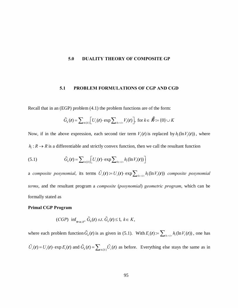
95
5.0 DUALITY THEORY OF COMPOSITE GP
5.1 PROBLEM FORMULATIONS OF CGP AND CGD
Recall that in an (EGP) problem (4.1) the problem functions are of the form:Equation Chapter 5 Section 1
[ ]
ˆ( ) ( ) exp ( ) , for : {0}k i li k l iG U V k K K
∈ ∈< > = ⋅ ∈ = ∪ ∑ ∑% t t t
Now, if in the above expression, each second tier term ( )lV t is replaced by (ln ( ))l lh V t , where
:lh R R→ is a differentiable and strictly convex function, then we call the resultant function
(5.1) [ ]
( ) ( ) exp (ln ( ))k i l li k l iG U h V
∈ ∈< > = ⋅ ∑ ∑t t t%
a composite posynomial, its terms ( ) : ( ) exp (ln ( ))i i l ll iU U h V
∈< >= ⋅ ∑t t t% composite posynomial
terms, and the resultant program a composite (posynomial) geometric program, which can be
formally stated as
Primal CGP Program
(CGP) 0 inf ( ) . . ( ) 1, ,m kRG s t G k K
∈≤ ∈% %
0<tt t
where each problem function ( )kG t% is as given in (5.1). With ( ) : (ln ( ))i l ll iE h V
∈< >= ∑t t , one has
[ ]( ) ( ) exp ( ) and ( ) ( )i i i k ii k
U U E G U∈
= ⋅ = ∑t t t t t%% % as before. Everything else stays the same as in

96
(EGP): the index sets { } { }{1,..., }, {1,..., }, 1, , , and 1, ,I n J m K p L r= = = =L L together with
their partition structures:
ˆ [ ], i Ik K i II k L i i+ ∈∈ ∈
= ∪ = ∪ < >= ∪ < >
{ }where : |I i I i+ = ∈ < >≠ φ , the sub-index sets [k] and i< > having 0 and 0k in r> ≥ number of
elements, respectively, the exponent matrixA
MB
=
, where [ ] : , [ ]:ij ljA a n m B b r m= × = × , and
the data matrixA cB d
, where ln , , ln , i i l lc C i I d D l L= ∈ = ∈ all are the same as in Chapter 4.
The only thing extra is a list of differentiable and strictly convex functions : ,lh R R l L→ ∀ ∈ . So
the problem is identifiable by an 8-tuple ( , , , , , , , )m n r p A B c d plus a list of functions: 1, , rh hL as
well as the partition structures of I and L. Clearly, the previous program (EGP) is a special case
of this program if exp,lh l L= ∀ ∈ . This generalization of (EGP) opens the door to model many
more applications. As before,
when , we regard ( ) 0, and ( ) ( )i i ii I E U U+∉ = =t t t%
when[ ]
[ ] , ( ) ( ) : ( )k i ki kk I G U G+
∈∩ = φ = =∑% t t t
When ˆ0, , , , ( ) ( ), ,k kr L i i I G G k K= = φ < >= φ ∀ ∈ = ∀ ∈% t t this reduces to a posynomial program
GP. The underlying (GP) of this (CGP) is meant to be the program when the entire list of second
tier terms ( )lV t are dropped off, i.e. when L = φ , and it is identifiable by a 5-tuple ( , , , , )m n p A c .
We shall assume here that 1 0nr r r= +…+ > so that (CGP) is not merely a GP problem.
If we take the logarithm of all problem functions in (CGP) and express them in the
logarithm of the design variables tj, we arrive at an equivalent program:

97
A convex form of (CGP) in the variables =: ln ,j jz t j J∈
(CGP)z 0 inf ( ) . . ( ) 0, m kRg s t g k K
∈≤ ∀ ∈% %
zz z ,
where the problem functions
(5.2) ( ){ }[ ]ˆ( ) : ln ( ) ln exp , i l
k k i l li k l ig G c h d k K
∈ ∈< > = = + + + ∀ ∈ ∑ ∑z t a z b z%%
are clearly differentiable (recall that , , : lni l
i lc di l l lU e V e d D+ += = =a z b z , and lb is the lth row of
the matrix B).
It is known that the composition of some posynomials with positive exponents can be
easily reformulated as a GP [Duffin et.al. pp. 96-97]. Although here the problem functions kg%
are also of composite type, these composite functions are defined on the z-space, not on the t-
space. Specifically, each kg% is a composite of the geometric function : kngeo R R→ with a
mapping : knmR R→ whose components ( ), [ ]ii l ll i
c h d i k∈< >
+ + ∀ ∈∑ la z b z + are clearly convex
in z. Hence by proposition 2.3.1 ( )kg z% is convex.
In terms of the variables , = , =: i lx i I l Lξ= ⇔ ∈ ∈i lx = Az ξ Bz a z, b z, , one has
(5.3) ( ){ } [ ] [ ][ ]
( ) ln exp ( , )k k k kk i i l l li k l i
g x c h d geoξ∈ ∈< >
= + + + = + + ∑ ∑z x c ξ d% % ,
where geo% is the composite geometric function we defined in (4.6). Thus we obtain an
equivalent form of CGP problems:
GGP form of (CGP) in the variables =: , and =: .i lx i I l Lξ∈ ∈i la z, b z,
(CGP)x,� 0 0 [0] [0] [ ] [ ]
( )inf ( , ) . . ( , ) 0, , ( )
n r
k k k k
R Rgeo s t geo k K
∈ ×+ + + + ≤ ∀ ∈ ∈
x,x c ξ d x c ξ d x,ξ% %
ξP

98
where the primal space P is the same as in (EGP): the column space of the exponent matrix M.
The variables in the problem functions [ ] [ ]( , )k k k kgeo + +x c ξ d% are also separated for different
ˆk K∈ .
Problem formulation of (CGD)
The format of dual program (CGD) is basically the same as that of the dual program
(EGD), where the dual variables and i ly η correspond to the first and second tier terms
( ) and ( )i lU Vt t% , respectively. As before 1 1 [ ] , [ ]n ri n l ry R Rη= ∈ = ∈y η , and the dual program is
also defined as:
(5.4) (CGD) *sup ( , ) : exp[ ( , )]
. . ( , ) =dual space of (CGD)V l
s tλ = −
∈
y yy
%% η ηη D
where *( )lλ y,η% is the conjugate of the Lagrangian ( , ) ( ; )l lλ =x ξ x,ξ% % λ of(CGP)x,ξ and : ⊥=D P =
null space of MT, that is, ( , )y η must satisfy T TA B+ =y 0η , or equivalently:
1 1
0, n r
ij i lj li l
a y b j Jη= =
+ = ∀ ∈∑ ∑ (Orthogonality conditions)
Proposition 5.1.1 The dual objective of (CGD) is
(5.5)
*
ˆ [ ]
0[ ]
( , ) exp ( / )
ˆif 0, , , 1, and , ,
otherwise, its value is 0,
iy
i kl l i l l i
l ii kk K i Ii
i i k l i li k
CV d y h yy
y y k K y J l i i I
λ η η
λ λ η
+ ∈< >∈∈ ∈
+∈
= ⋅ −
≥ = ∀ ∈ = ∈ ∀ ∈< > ∈
∑ ∑∏∏
∑
y% η
where, lJ is the domain interval of the conjugate function * lh .
Proof: The Lagrangian of (CGP)x,ξ is
[ ] [ ]0ˆ( ; ) ( , ), with 1k k k k
kk Kl geoλ λ
∈= + + =∑x,ξ x c ξ d% %λ

99
Its conjugate, by (4.9), is
* *ˆ [ ] [ ]
( ) ln( / ) ( / )i i i k i l l i l lk K i k i k l il y y C y h y dλ λ η η+∈ ∈ ∈ ∈< >
= + − ∑ ∑ ∑ ∑y,η% ,
0[ ]ˆif 0, , , 1, and , , ;otherwise, its value is .i i k l i li k
y y k K y J l i i Iλ λ η +∈
≥ = ∀ ∈ = ∈ ∀ ∈< > ∈ ∞∑
So the dual objective of (CGD) is
* *
ˆ [ ]
( , ) exp[ ( , )] exp ( / )iy
i kl l i l l i
l ii kk K i Ii
CV l d y h yyλλ η η
+ ∈< >∈∈ ∈
= − = ⋅ −
∑ ∑∏∏y y%% η η ,
with the above-mentioned restrictions.
∎
Thus the dual program (CGD) can be elaborated as
Dual program (CGD) (Under the convention: 0 *0 1, 0 ( / 0) ( | 0)l l lh iη η= = )
(5.6) (CGD)
*
ˆ( ) [ ]
0
1 1
sup ( , ) : exp ( / )
. . 1, (Normality Condition)
0, (
i
n r
y
i kl l i l l i
R R l ii kk K i Ii
n r
ij i lj li l
CV d y h yy
s t
a y b j J
λ η η
λ
η
+∈ × ∈< >∈∈ ∈
= =
= ⋅ −
=
+ = ∈
∑ ∑∏∏
∑ ∑
% ηy,η
y
[ ]
Orthogonality Conditions)
ˆ 0, , ,
, , (*)
i i ki k
l i l
y i I y k K
y J l i i I
λ
η∈
+
≥ ∀ ∈ = ∀ ∈
∈ ∀ ∈< > ∈
∑
The domain conditions in (*) constraints are sublinear, hence potentially nonlinear, but they will
be fulfilled if a pair of primal and dual solutions ( ; , )t y η satisfy the extremality condition to be
described in equation (5.10) (b). In particular, they imply that
(5.7) 0 0, , i ly l i i Iη += ⇒ = ∀ ∈< > ∈
The convention * 0 ( / 0) ( | 0)l l lh iη η= implies that ( , ) 0, if , . . 0, 0i lV l i s t y η= ∃ ∈< > = ≠% y η

100
As with (EGD), the underlying (GD) of this (CGD) is meant to be the program where the
second tier vector variableη , the constant vector d , and the matrix B are all absent from (CGD),
i.e. set L = φ . This program is then the geometric dual of the underlying (GP).
The dual functions ( , ) and V y V(y)% η satisfy
(5.8) *( , ) ( ) exp ( / )l l i l l il ii I
V V d y h yη η+ ∈< >∈
= ⋅ −
∑ ∑% y yη
and their respective log-dual functions ( , ) ln ( , ) and ( ) ln ( )v V v V= =%% y y y yη η satisfy:
(5.9) *( , ) ( ) ( / )l l i l l il ii I
v v d y h yη η+ ∈< >∈
= + − ∑ ∑% y yη .
As already pointed out in chapter 4, this function ( , )v% y η is usc proper and concave.
So the dual program (CGD) is also equivalent to a convex program with (m+1) linear
equality constraints and non-negativity conditions on its n dual variables iy , except for except for
those constraints in (*). Its degree of difficulty d is also defined as the number 1n r m+ − − ,
which is usually the dimension of its dual flat. This number is r greater than that of its
underlying GD, because CGP is a more complex model than its underlying GP, containing r
more posynomial terms in the second tier.
Just like the EGD case, the log-dual program of (CGD) also possesses 3 exploitable
structures: concavity, partial-separability, and linearity that are originally hidden in the (CGP)
model. Obviously, these features would make solving the primal through its dual an attractive
approach, provided that the two programs have identical optimal values and conversion of
optimum solutions from dual to primal is computationally economical. As in the precious
chapter, the duality theory of CGP attempts to confirm the above fact under mild conditions.
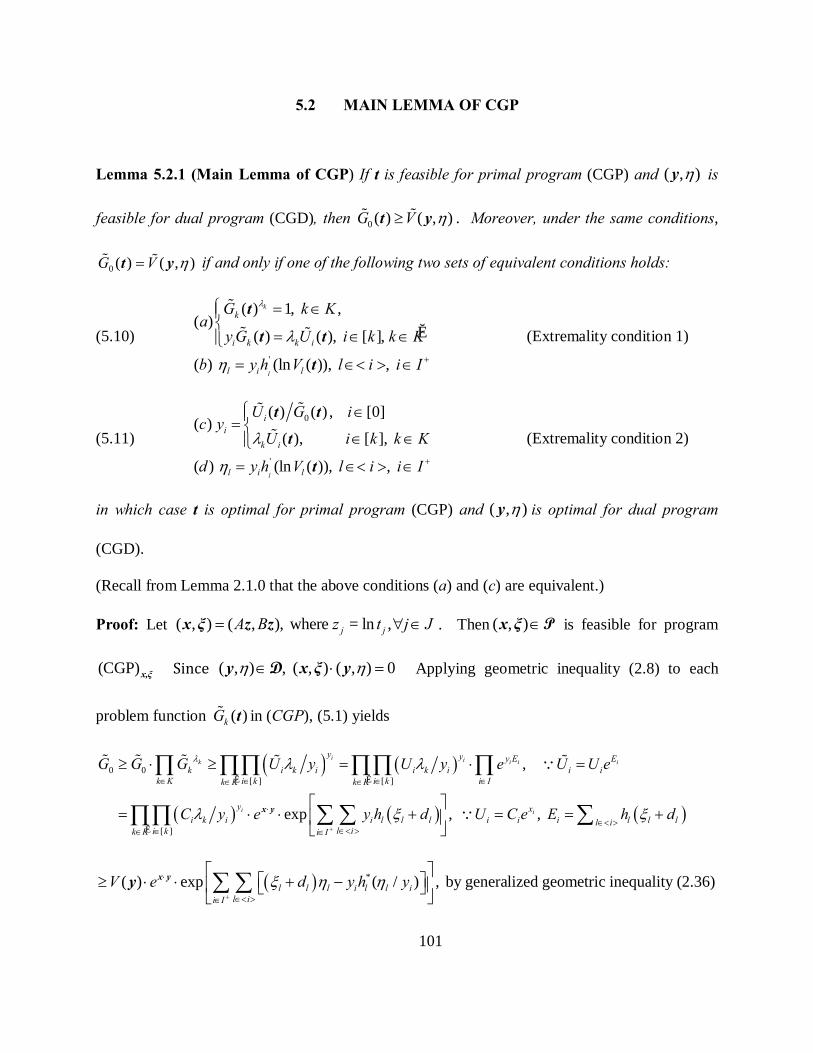
101
5.2 MAIN LEMMA OF CGP
Lemma 5.2.1 (Main Lemma of CGP) If t is feasible for primal program (CGP) and ( , )y η is
feasible for dual program (CGD), then 0 ( ) ( , )G V≥% %t y η . Moreover, under the same conditions,
0 ( ) ( , )G V=% %t y η if and only if one of the following two sets of equivalent conditions holds:
(5.10) '
( ) 1, , ( )
ˆ( ) ( ), [ ],
( ) (ln ( )), ,
k
l
k
i k k i
l i l
G k Ka
y G U i k k K
b y h V l i i I
λ
λ
η +
= ∈
= ∈ ∈= ∈< > ∈
t
t t
t
%
% % (Extremality condition 1)
(5.11) 0
'
( ) ( ) , [0] ( )
( ), [ ],
( ) (ln ( )), , l
ii
k i
l i l
U G ic y
U i k k K
d y h V l i i I
λ
η +
∈= ∈ ∈
= ∈< > ∈
t t
t
t
%%%
(Extremality condition 2)
in which case t is optimal for primal program (CGP) and ( , )y η is optimal for dual program
(CGD).
(Recall from Lemma 2.1.0 that the above conditions (a) and (c) are equivalent.)
Proof: Let ( , ) ( , ), where = ln ,j jA B z t j J= ∀ ∈x ξ z z . Then ( , )∈x ξ P is feasible for program
(CGP)x,ξ Since ( , ) , ( , ) ( , ) 0∈ ⋅ =y x ξ yη ηD Applying geometric inequality (2.8) to each
problem function ( )kG t% in (CGP), (5.1) yields
( ) ( )
( ) ( ) ( )
0 0ˆ ˆ[ ] [ ]
ˆ [ ]
,
exp , ,
i ik i i i
i i
y y y E Ek i k i i k i i i
k K i k i k i Ik K k K
y xi k i i l l l i i i l l ll i
l ii kk K i I
G G G U y U y e U U e
C y e y h d U C e E h d
λ λ λ
λ ξ ξ+
∈ ∈ ∈ ∈∈ ∈
⋅∈< >
∈< >∈∈ ∈
≥ ⋅ ≥ = ⋅ =
= ⋅ ⋅ + = = +
∏ ∏∏ ∏∏ ∏
∑ ∑ ∑∏∏
% % % % %∵
∵x y
( ) *( ) exp ( / ) , by generalized geometric inequality (2.36)l l l i l l il ii I
V e d y h yξ η η+
⋅
∈< >∈
≥ ⋅ ⋅ + −
∑ ∑x yy

102
* ( ) exp ( / )l l i l l il ii I
V e e d y h yη η+
⋅ ⋅
∈< >∈
= ⋅ ⋅ ⋅ −
∑ ∑x y ξy η
* ( ) exp ( / ) , 0
( , )
l l i l l il ii I
V d y h y
V
η η+ ∈< >∈
= ⋅ − ⋅ + ⋅ =
=
∑ ∑ ∵
%
y x y ξ
y
η
η
Therefore, 0 ( ) ( , )G V≥% %t y η and conditions for equality in the last inequality are
' ( ), , ll i l ly h d l i i Iη ξ += + ∈< > ∈ , which are the same as ' (ln ( )), ,
ll i ly h V l i i Iη += ∈< > ∈t , and
this is condition (b) of (5.10). Therefore, equality holds iff the extremality conditions (5.10) or
(5.11) are satisfied. ∎
Alternate proof Assume that we have ( , ) and ( , )∈ ∈x ξ y ηP D feasible for program(CGP)x,ξ
and (CGD), respectively, thus ( , ) ( , )⊥x ξ y η and
(5.12) 0 0 [0] [0] [ ] [ ]0ˆ( , ) ( , ) ( , ), where 1k k k k
kk Kgeo geo lλλ λ
∈+ + ≥ + + = =∑x c ξ d x c ξ d x ξ%% %
with equality holding iff [ ] [ ]( , ) 0,k k k kk geo k Kλ + + = ∀ ∈x c ξ d% .
In (CGP)x,ξ , each problem function
( ){ }[ ] [ ][ ]
ˆ( , ) ln exp ,k k k ki i l l li k l i
geo x c h d k Kξ∈ ∈< >
+ + = + + + ∀ ∈ ∑ ∑x c ξ d%
has partial derivatives:
(5.13) ' ( ) ( ) ˆ, [ (ln ( ))], , [ ],( ) ( ) l
i il
i lk k
U U h V l i i k k Kx G Gξ
∂ ∂= = ∀ ∈< > ∀ ∈ ∀ ∈ ∂ ∂
t t tt t
% %% %
Apply (2.33) to each function [ ] [ ] ˆ( , ), k k k kk geo k Kλ + + ∈x c% ξ d using (4.9) to get
(5.14) [k] [k] *
[ ] [ ]
[ ]
( , ) ln( / ) ( / )
ˆ ,
k kk i i i k i l l i l li k i k l i
i i l li k l i
geo y y C y h y d
x y k K
λ λ η η
ξ η
+∈ ∈ ∈< >
∈ ∈< >
+ + + −
≥ + ∀ ∈
∑ ∑ ∑∑ ∑
x c ξ + d%
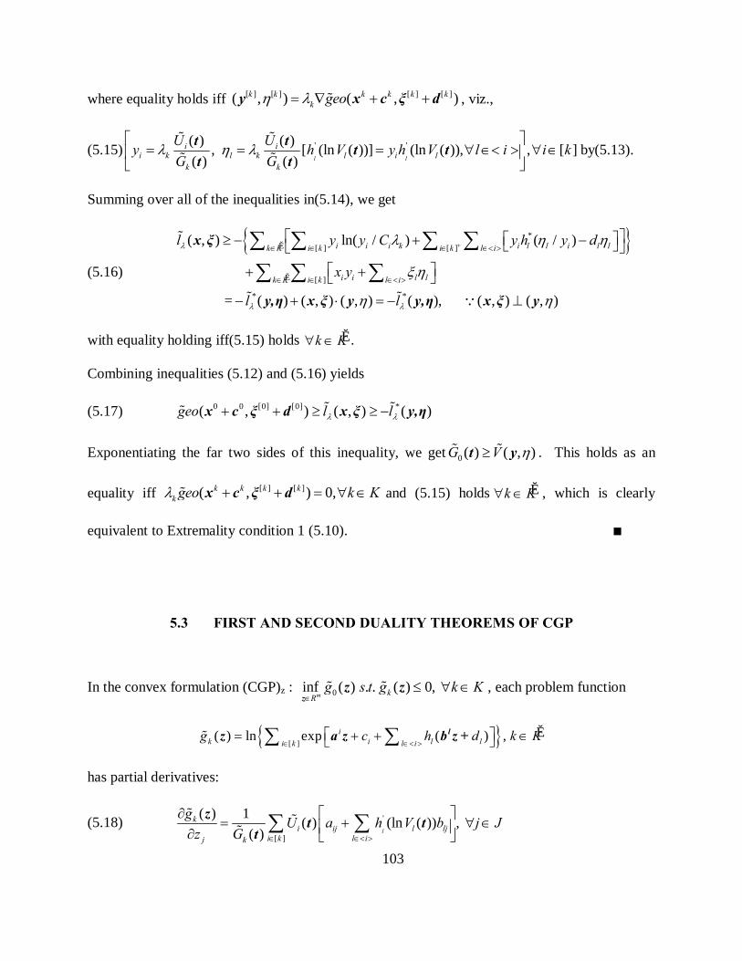
103
where equality holds iff [ ] [ ] [ ] [ ]( , ) ( , )k k k k k kk geoλ= ∇ + +%y x c ξ dη , viz.,
(5.15) ' ' ( ) ( ), [ (ln ( ))] (ln ( )), , [ ] ( ) ( ) l l
i ii k l k l i l
k k
U Uy h V y h V l i i kG G
λ η λ
= = = ∀ ∈< > ∀ ∈
t t t tt t
% %% % by(5.13).
Summing over all of the inequalities in(5.14), we get
(5.16)
{ }*ˆ [ ] [ ]
ˆ [ ]
* *
( , ) ln( / ) ( / )
= ( ) ( , ) ( , ) ( ), ( , ) ( , )
i i i k i l l i l lk K i k i k l i
i i l lk K i k l i
l y y C y h y d
x y
l l
λ
λ λ
λ η η
ξ η
+∈ ∈ ∈ ∈< >
∈ ∈ ∈< >
≥ − + −
+ +
− + ⋅ = − ⊥
∑ ∑ ∑ ∑∑ ∑ ∑
x ξ
y,η x ξ y y,η x ξ y
%
% % ∵η η
with equality holding iff(5.15) holds ˆk K∀ ∈ .
Combining inequalities (5.12) and (5.16) yields
(5.17) 0 0 [0] [0] *( , ) ( , ) ( )geo l lλ λ+ + ≥ ≥ −x c ξ d x ξ y,η% %%
Exponentiating the far two sides of this inequality, we get 0 ( ) ( , )G V≥% %t y η . This holds as an
equality iff [ ] [ ]( , ) 0,k k k kk geo k Kλ + + = ∀ ∈x c ξ d% and (5.15) holds ˆk K∀ ∈ , which is clearly
equivalent to Extremality condition 1 (5.10). ∎
5.3 FIRST AND SECOND DUALITY THEOREMS OF CGP
In the convex formulation (CGP)z : 0 inf ( ) . . ( ) 0, m kR
g s t g k K∈
≤ ∀ ∈% %z
z z , each problem function
{ }[ ]ˆ( ) ln exp ( ) , i
k i l li k l ig c h d k K
∈ ∈< > = + + ∈ ∑ ∑ lz a z b z +%
has partial derivatives:
(5.18) '
[ ]
( ) 1 ( ) (ln ( )) , ( ) l
ki ij l lj
i k l ij k
g U a h V b j Jz G ∈ ∈< >
∂ = + ∀ ∈ ∂ ∑ ∑z t t
t% %
%
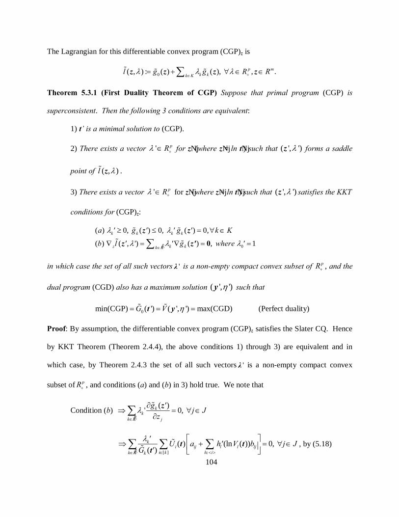
104
The Lagrangian for this differentiable convex program (CGP)z is
0( , ) : ( ) ( ), , .p mk kk K
l g g R Rλ +∈= + ∀ ∈ ∈∑z z z z% % %λ λ
Theorem 5.3.1 (First Duality Theorem of CGP) Suppose that primal program (CGP) is
superconsistent. Then the following 3 conditions are equivalent:
1) t’ is a minimal solution to (CGP).
2) There exists a vector ' pR+∈λ for z′ (where z′= ln t′) such that ( ', ')z λ forms a saddle
point of ( , )l z% λ .
3) There exists a vector ' pR+∈λ for z′ (where z′= ln t′) such that ( ', ')z λ satisfies the KKT
conditions for (CGP)z:
0ˆ
( ) 0, ( ) 0, ( ) 0,
( ) ( , ') ( ) , 1k k k k
z k kk K
a ' g ' ' g ' k K
b l ' ' g where '
λ λ
λ λ∈
≥ ≤ = ∀ ∈
∇ = ∇ = =∑ 0
% %% %
z z
z z'λ
in which case the set of all such vectors 'λ is a non-empty compact convex subset of pR+ , and the
dual program (CGD) also has a maximum solution ( ', ')y η such that
0min(CGP) ( ') ( ', ') max(CGD)G V= = =% %t y η (Perfect duality)
Proof: By assumption, the differentiable convex program (CGP)z satisfies the Slater CQ. Hence
by KKT Theorem (Theorem 2.4.4), the above conditions 1) through 3) are equivalent and in
which case, by Theorem 2.4.3 the set of all such vectors 'λ is a non-empty compact convex
subset of pR+ , and conditions (a) and (b) in 3) hold true. We note that
Condition (b) ˆ
( )' 0, kk
k K j
g ' j Jz
λ∈
∂⇒ = ∀ ∈
∂∑ % z
ˆ [ ]
( ) (ln ( )) 0, ( )k
i ij l l lji k l ik K k
' U a h' V b j JG '
λ∈ ∈< >∈
⇒ + = ∀ ∈ ∑ ∑ ∑%
% t tt
, by (5.18)

105
Now define ˆ( ) / ( ) 0, [ ], ; and (ln ( )), , .i k i k i i l ly ' 'U ' G ' i k k K ' y 'h' V ' l i i Iλ η += ≥ ∀ ∈ ∀ ∈ = ∈< > ∈%% t t t
Then condition (*) in (CGD): , , l i ly J l i i Iη +∈ ∀ ∈< > ∈ is satisfied (∵ *range ( ) dom llh' h⊂ )
and we have
ˆ [ ] 1 1
0, n r
ij i lj l ij i lj li k l i i lk K
a y ' b ' a y ' b ' j Jη η∈ ∈< > = =∈
+ = + = ∈ ∑ ∑ ∑ ∑ ∑
which are the orthogonality conditions for (CGD). It is then easy and routine to check that the
above given ( ', ')y η is a dual feasible solution, which together with t′ satisfy the extremality
condition (5.10). Therefore, by main lemma of (CGP), this ( ', ')y η is a maximum solution
satisfying 0min(CGP) ( ') ( ', ') max(CGD)G V= = =t y% % η ∎
Since in (CGP)z the problem functions are [ ] [ ]( ) ( , )k k k kkg geo= + +z A z c B z d% % ,
[ ]
[ ]( ) ( , ) max ( )
l
k kk l ii k
g geo h∞ ∞ ∞∈< >∈
= = + ∑i lz A z B z a z b z% % , by (4.24)
The directions of recession of (CGP)z are the nontrivial solutions to the system:
(5.19)
ˆ ˆ( ) 0, ( ) 0, [ ],
( ) 0,
( )
lk l ii
i
g k K h i k k K
H i I
H
∞ ∞∈< >
∞
∞
≤ ∀ ∈ ⇔ + ≤ ∀ ∈ ∀ ∈
⇔ + ≤ ∀ ∈
⇔ + ≤
∑i l
i
z a z b z
a z B zAz Bz 0
%
Since in general we do not know the exact form of the dual linear system of inequalities
to the above system (this depends on the nature of all the functions lh that are involved), we
cannot provide a general duality theorem here. We can however, supply an existence theorem.
Theorem 5.3.2 (Existence Theorem of CGP) Suppose that primal program (CGP) is
consistent. Then the minimum set of program (CGP)z is non-empty and bounded if and only if
the system ( )H ∞+ ≤Az Bz 0 has no nontrivial solutions in z.

106
6.0 DUALITY THEORY OF QUADRATIC GP
The content of the duality theory of QGP to be presented in this chapter is independent of
the material in chapters 4 and 5. However, in chapter 7, we shall present a more general and
elegant approach to the same theory but this time as a special case of the duality theory of CGP
developed in Chapter 5. In this way one can contrast the two different approaches to the same
subject.Equation Chapter (Next) Section 1
6.1 PROBLEM FORMULATIONS OF QGP
We define a quadratic geometric program (QGP) as follows: First, the index sets
{ } { }{1,..., }, {1,..., }, 1, , , and 1, ,I n J m K p L r= = = =L L together with the partition structures:
ˆ ˆ [ ][ ], i I i kk K k Ki II k L i i i+ ∈ ∈∈ ∈∈
= ∪ = ∪ < >= ∪ < > = ∪ ∪ < >
{ } { }where : | 0 |iI i I r i I i+ = ∈ > = ∈ < >≠ φ , are the same as in (EGP) (Chapter 4). Each index
subset <i> has ir (≥0) elements, { }1 1, , ,i ii S S i I−< >= + ∀ ∈L , where 1 : , and i iS r r i I= +…+ ∀ ∈
0 0S = .

107
Primal program (QGP)
(QGP) 0 inf ( ) . . ( ) 1, ,m kRG s t G k K
∈≤ ∈% %
0<tt t
with
(6.1) [ ]
212
ˆ( ) ( ), ( ) : ( ) exp ( ), ( ) ,
( ) : ln ( ), and ( ) , ,
ij
lj
ak i i i i i i ji k j J
bi l l l jl i j J
G U U U H U C t k K
H V V D t l i i I∈ ∈
+∈< > ∈
= = ⋅ = ∈
= = ∀ ∈< > ∀ ∈
∑ ∏∑ ∏
t t t t t t
t t t
% % %
For easy reference, we adopt the name given by Hough (1978) and call ( )iU t% a Quadratic
Posylognomial (QPL) term, when ( 0)ii I i r+∈ ⇔< >≠ φ ⇔ > , and call ( )kG t% a Quadratic
Posylognomial, when[ ]k I +∩ ≠ φ . The exponent matrix for this program isA
MB
=
, where
[ ] : , [ ]:ij ljA a n m B b r m= × = × . The data for this program is the ( ) ( 1)n r m+ × + matrix A cB d
and the partition structures of I and L, where ln , , ln , i i l lc C i I d D l L= ∈ = ∈ .
When , we may regard ( ) 0, and ( ) ( )i i ii I H U U+∉ = =t t t% .
When[ ]
[ ] , ( ) ( ) : ( ).k i ki kk I G U G+
∈∩ = φ = =∑% t t t
When ˆ( 0), ( ) ( ),k kI L r G G k K+ = φ ⇔ = φ ⇔ = = ∀ ∈% t t ,
then our program reduces to a posynomial program GP. By the underlying (GP) of this (QGP)
we mean the program where all of the second tier terms ( )lV t are absent ( 0)r⇔ = . Since
( ) 0iH ≥t , we have ( ) ( ), , ( ) ( ), ,i i k kU U i G G k≥ ∀ ≥ ∀%% t t t t thus inf inf .QGP GP≥ We assume here
that 1 0nr r r= +…+ > so that (QGP) is not merely a GP problem.

108
A convex form of (QGP) in the variables =: ln ,j jz t j J∈
0( ) inf ( ) . . ( ) 0, m kRQGP g s t g k K
∈≤ ∀ ∈% %z z
z z ,
where the problem functions
(6.2) { }212[ ]
ˆ( ) : ln exp | | , i lk i li k l i
g c d k K∈ ∈< >
= + + + ∈ ∑ ∑% z a z b z
are clearly convex (recall that , , : lni l
i lc di l l lU e V e d D+ += = =a z b z , and lb is the lth row of the
matrix B). These functions become those in equation (1.24), if 1, lD l L= ∀ ∈ , since
2 2|| || | |ll i∈< >
= ∑iB z b z , where lb is a row of the matrix iB . So our (QGP) model is slightly more
flexible than the (QPL) model studied by previous researchers. It is worth noting that if the
coefficient ½ that appears in the (QGP) model formula for ( )kG% t or for ( )kg% z is any other
positive constant, say ls , the program is still convertible to a QGP problem by simply multiplying
the lth row [ lldb ] of the data matrix [ ]B d by 2 ls , since ( ) ( ) 22 1
2 2l ll l l ls d s d + = + b z b z .
A GGP reformulation of (QGP) in the variables =: , =: .i lx i I l Lξ∈ ∈i la z, b z,
(QGP)x,� 0( )
inf ( ) . . ( ) 0, , ( , )n r kR
g s t g k K+∈
≤ ∀ ∈ ∈% %x,
x,ξ x,ξ x ξξ
P ,
where P (the primal space of this program) is the column space of the exponent matrix M, and
the variables in these convex problem functions
(6.3) { }212[ ]
( ) : ln exp | | ,k i i l li k l ig x c dξ
∈ ∈< > = + + + ∑ ∑x,ξ%
are separated for different ˆk K∈ .
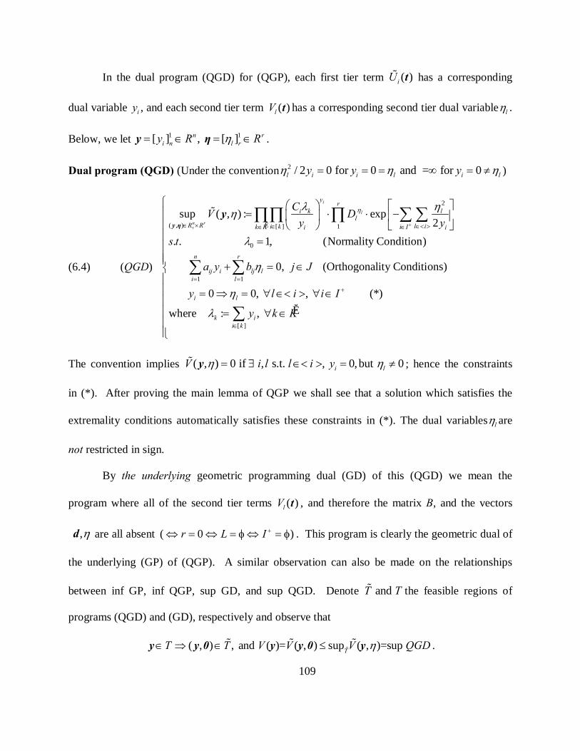
109
In the dual program (QGD) for (QGP), each first tier term ( )iU% t has a corresponding
dual variable iy , and each second tier term ( )lV t has a corresponding second tier dual variable lη .
Below, we let 1 1 [ ] , [ ]n ri n l ry R Rη= ∈ = ∈y η .
Dual program (QGD) (Under the convention 2 / 2 0 for 0 and = for 0l i i l i ly y yη η η= = = ∞ = ≠ )
(6.4) (QGD)
2
ˆ( , ) [ ] 1
0
1 1
sup ( , ) : exp 2
. . 1, (Normality Condition)
0, (Ortho
i
l
n r
y ri k l
lR R l ii kk K i Ii i
n r
ij i lj li l
CV Dy y
s t
a y b j J
ηλ η
λ
η
++∈ × ∈< >∈∈ ∈
= =
= ⋅ ⋅ −
=
+ = ∈
∑ ∑∏∏ ∏
∑ ∑
%y η
y η
[ ]
gonality Conditions)
0 0, , (*) ˆwhere : ,
i l
k ii k
y l i i I
y k K
η
λ
+
∈
= ⇒ = ∀ ∈< > ∀ ∈ = ∀ ∈
∑
The convention implies ( , ) 0 if , s.t. , 0, but 0i lV i l l i y η= ∃ ∈< > = ≠% y η ; hence the constraints
in (*). After proving the main lemma of QGP we shall see that a solution which satisfies the
extremality conditions automatically satisfies these constraints in (*). The dual variables lη are
not restricted in sign.
By the underlying geometric programming dual (GD) of this (QGD) we mean the
program where all of the second tier terms ( )lV t , and therefore the matrix B, and the vectors
,d η are all absent ( 0 )r L I +⇔ = ⇔ = φ ⇔ = φ . This program is clearly the geometric dual of
the underlying (GP) of (QGP). A similar observation can also be made on the relationships
between inf GP, inf QGP, sup GD, and sup QGD. Denote and T T% the feasible regions of
programs (QGD) and (GD), respectively and observe that
( , ) , and ( )= ( , ) sup ( , )=sup TT T V V V QGD∈ ⇒ ∈ ≤y y 0 y y 0 y%% % % η .
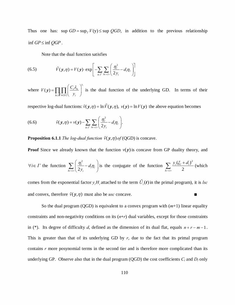
110
Thus one has: sup sup (y) sup ,TGD V QGD= ≤ in addition to the previous relationship
inf infGP QGP≤ .
Note that the dual function satisfies
(6.5) 2
( , ) ( ) exp2
ll l
l ii I i
V V dy
η η+ ∈< >∈
= ⋅ − −
∑ ∑% y yη
where ˆ [ ]
( )iy
i k
i kk K i
CVyλ
∈∈
=
∏∏y is the dual function of the underlying GD. In terms of their
respective log-dual functions: ( , ) ln ( , ), ( ) ln ( )v V v V= =%% y y y yη η the above equation becomes
(6.6) 2
( , ) ( )2
ll l
l ii I i
v v dy
η η+ ∈< >∈
= − −
∑ ∑% y yη .
Proposition 6.1.1 The log-dual function ( , )v% y η of (QGD) is concave.
Proof Since we already known that the function ( )v y is concave from GP duality theory, and
i I +∀ ∈ the function 2
2l
l ll i i
dy
η η∈< >
−
∑ is the conjugate of the function
2( )2
i l l
l i
y dξ∈< >
+∑ (which
comes from the exponential factor i iy H attached to the term ( )iU t% in the primal program), it is lsc
and convex, therefore ( , )v% y η must also be usc concave. ∎
So the dual program (QGD) is equivalent to a convex program with (m+1) linear equality
constraints and non-negativity conditions on its (n+r) dual variables, except for those constraints
in (*). Its degree of difficulty d, defined as the dimension of its dual flat, equals 1n r m+ − − .
This is greater than that of its underlying GD by r, due to the fact that its primal program
contains r more posynomial terms in the second tier and is therefore more complicated than its
underlying GP. Observe also that in the dual program (QGD) the cost coefficients Ci and Dl only

111
appear in its objective function and the technological coefficients aij and blj only in the
constraints; whereas in (QGP) they are scattered all over the terms ( )iU t% of the functions ( )kG t% .
The log-dual program (QGD) possesses 3 exploitable structures: concavity, partial-separability,
and linearity that are originally hidden in the (QGP) model. Obviously, these features would
make solving the primal through its dual an attractive approach, provided that the two programs
have identical optimal values and conversion of optimum solutions from dual to primal is not
computationally economical. The duality theory of QGP confirms the above fact under mild
conditions.
6.2 MAIN LEMMA OF QGP
Similar to the EGP case, we also need an additional geometric inequality, which is related to the
quadratic function, to prove this lemma. Fenchel’s inequality for the quadratic function 212 ξ is:
2 21 12 2 , , with equality holding iff Rξ η ξη ξ η ξ η+ ≥ ∀ ∈ = .
Fenchel’s inequality for the function 212 ( )y dξ + with 0y ≥ (under the convention:
2 / (2 ) 0 for y=0= ; and =+ for y=0yη η η= ∞ ≠ ) is:
(6.7) 2 2( ) ( ) , , , ,
2 2y d d d R y R
yξ η ξ η ξ η +
++ ≥ + ∀ ∈ ∈ ,
with equality holding iff ( ) iff / , when 0y d d y yη ξ ξ η= + + = > .
Lemma 6.2.1 (Main Lemma of QGP) If t is feasible for primal program (QGP) and ( , )y η is
feasible for dual program (QGD), then 0 ( ) ( , )G V≥t% % y η
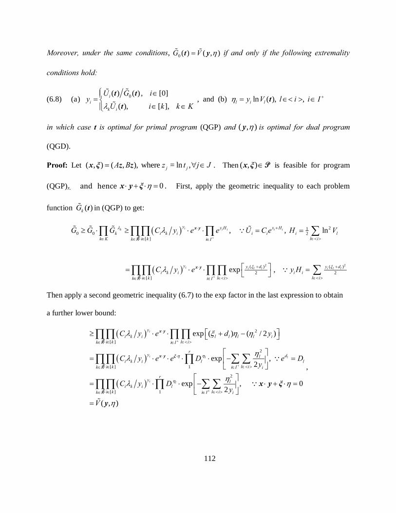
112
Moreover, under the same conditions, 0 ( ) ( , )G V=% %t y η if and only if the following extremality
conditions hold:
(6.8) 0( ) ( ) , [0] (a) , and (b) ln ( ), ,
( ), [ ], i
i l i lk i
U G iy y V l i i I
U i k k Kη
λ+
∈= = ∈< > ∈∈ ∈
%%%t t
tt
in which case t is optimal for primal program (QGP) and ( , )y η is optimal for dual program
(QGD).
Proof: Let ( , ) ( , ), where = ln ,j jA B z t j J= ∀ ∈x ξ z z . Then ( , )∈x ξ P is feasible for program
(QGP)x,� and hence 0⋅ + ⋅ =x y ξ η . First, apply the geometric inequality to each problem
function ( )kG t% in (QGP) to get:
( ) 21
0 0 2ˆ [ ]
, , ln
ik i i i iy y H x H
k i k i i i i ll ik K i kk K i I
G G G C y e e U C e H Vλ λ+
+⋅
∈< >∈ ∈∈ ∈
≥ ⋅ ≥ ⋅ ⋅ = = ∑∏ ∏∏ ∏% % % %∵x y
( )2 2( ) ( )
2 2ˆ [ ]
exp , i i l l i l ly y d y di k i i i
l ii k l ik K i I
C y e y Hξ ξλ+
+ +⋅
∈< >∈ ∈< >∈ ∈
= ⋅ ⋅ = ∑∏∏ ∏ ∏ ∵x y
Then apply a second geometric inequality (6.7) to the exp factor in the last expression to obtain
a further lower bound:
( )
( )
( )
2
ˆ [ ]
2
ˆ [ ] 1
2
ˆ [ ] 1
exp ( ) ( / 2 )
exp , 2
exp , 2
i
i l l
i l
yi k i l l l l i
i k l ik K i I
ry dl
i k i l ll ii kk K i I i
ry l
i k i ll ii kk K i I i
C y e d y
C y e e D e Dy
C y Dy
η
η
λ ξ η η
ηλ
ηλ
+
+
+
⋅
∈ ∈< >∈ ∈
⋅ ⋅
∈< >∈∈ ∈
∈< >∈∈ ∈
≥ ⋅ ⋅ + −
= ⋅ ⋅ ⋅ ⋅ − =
= ⋅ ⋅ −
∏∏ ∏ ∏
∑ ∑∏∏ ∏
∑ ∑∏∏ ∏
x y
x y ξ ∵η
0
( , )V
⋅ + ⋅ =
=
x y ξ
y
∵
%
η
η
,

113
and additional conditions for equality are ( ) ln ( ), , l i l l i ly d y V l i i Iη ξ += + = ∀ ∈< > ∈t , which
are the same as conditions (b) in the lemma(6.8). Therefore, 0 ( ) ( , )G V≥% %t y η and equality holds
iff the extremality conditions are satisfied. ∎
This main lemma clearly extends the earlier main lemma of GP.
Corollary 6.2.2 (Weak Duality Theorem for (QGP))
1) Always inf sup 0QGP QGD∞ ≥ ≥ ≥
2) When (QGP) and (QGD) are feasible, inf sup 0.QGP QGD∞ > ≥ >
Example 6.2.1 A (QGP) problem [Duffin et.al, p.214-5]
( )2 20 1 2 1 2 1 1 2 3 2 2 3 1 1 3 2 1 2min s.t. ln ln 1, where 4 / , 4 , 2 , U U V V U t t t U t t V t t V t t+ + ≤ = = = =t >
Since the constraint is equivalent to: 1 2 21 2exp ln ln 1e V V− + ≤ with 1
3 , 3 {1,2}U e−= < >= , it is
equivalent to a (QGP) problem with 3, 2, 3n r m= = = . ∎
Example 6.2.2 [Fang and Rajasekera, 1987] revisited
12
50ln 1 10 1 2 1 1 2
1/21 1 2
inf ( )( ) ,
. . ( ) 0.01 1,
t
RG t t t t t
QPLs t G t t
− −
∈ = ⋅ +
= + ≤
0%
<tt
t
In our QGP formulation, it is
( )2
2 1 110 1 2 1 1 22
1/21 1 2
inf ( ) exp ln ( )( )
. . ( ) 0.01 1, R
G t t V t tQGP
s t G t t
− −
∈ = ⋅ +
= + ≤
0%
<tt t
t
where 101 1 ( ) , 1 {1}V t= < >=t . So 4, 1, 2n r m= = = , the exponent matrix is
AM
B
=
, with
[ ]10 0B = , and A as is usual.

114
Its convex form is:
(QGP)z [ ]
2
210 1 2 1 1 22
11 1 22
inf ( ) ln exp( (10 ) ) exp( )
. . ( ) ln exp( 2ln10 ) exp( ) 0R
g z z z z z
s t g z z∈
= + + + − −
= − + + ≤
%z
z
z ∎
Dual to Primal conversion of optimum solutions
Suppose we have found an optimum solution ( , )vδ for the dual program (QGD), and want to
convert it to optimum solutions t for the primal program (QGP), believing that they have same
optimum values 0 ( ) ( , ) :G V V= =% t vδ . We can derive from (Extremality Condition 2) that
(6.9) , for [0]
( ), for [ ], , and 0
/ , and 0
ii
i k k
i ii i
V iU
i k k K
B v i I
δδ λ λ
δ δ
∈= ∈ ∈ >
= ∀ ∈ >
% t
z
Recall from that 212( ) exp{ | | }i i
i iU B c= + +% t z a z . Taking logarithms of both sides of the first set
of equations above and replacing Biz using the last equation yields
( )2
2
ln( ), for [0]| |ln , for [ ], , 0, and 02
iii
ii k i ki
V iv ci k k K
δδ λ δ λδ
∈+ + = ∈ ∈ > >a z
The last condition in (6.9) says , , if 0, /li l il i i I vδ δ∀ ∈< > ∈ > =b z .
So all optimum solutions z for (QGP)z must satisfy the following system of linear equations:
(6.10) ( )
2 2
2 21
1
ln( / ) | | / 2 for [0]
ln | | / 2 , for [ ], , 0, and 0
/ , for , s.t. 0
imi i i
ij j ij i i k i i k
m
lj j l i ij
V C v ia z
C v i k k K
b z v l i i I
δ δ
δ λ δ δ λ
δ δ
=
=
− ∈= − ∈ ∈ > >
= ∈< > ∈ >
∑
∑
Any solution z to the above system together with the given dual optimum solution ( , )vδ will
satisfy extremality condition 2 and ( ) 0, :{ | 0}k kg k K k K λ+= ∀ ∈ = ∈ >% z . If the coefficient

115
matrix of the above system has rank m, e.g., if the optimum solution ( , )vδ happens to have all
δi>0, and M has full column rank m, then the primal problem (QGP)z has a unique optimum
solution determined by the above system. If not, the optimum solutions z can still be
characterized by adjoining the equations: ( ) 0, \kg k K K +≤ ∀ ∈% z into the above system.
Observe that for the (GP) case equation (6.10) easily reduces to that of [Duffin et.al. 1967, p.
185].
6.3 FIRST AND SECOND DUALITY THEOREMS OF QGP
Just as in the case of GP, we call a QGP problem superconsistent if all of its constraints can be
satisfied strictly, i.e. there is a point t0 such that 0( ) 1kG <% t for all k in K. We define the
Lagrangian for (QGP)z: 0( , ) ( ) ( ), for , and .p mk kk K
l g g R Rλ +∈= + ∈ ∈∑% %z z z zλ λ
This corresponds to the product function we used in the proof of the main lemma for QGP
01
( , ) exp ( , ) ( ) ( ) k
p
kk
L l G G t λ
=
= = ∏% %t z tλ λ .
Similarly, the following formulae include equation as a special case.
(6.11)
[ ]
1( ) ( ) , ( ) ( )[( ) ]( )
i T i i T ii k i
i kk
u Q g U QG ∈
∇ = + ∇ = +∑ %% % %z a z z t a zt
Theorem 6.3.1 (First Duality theorem of QGP) Suppose that primal program QGP is
superconsistent. Then a point t′ is a minimum solution for (QGP) if and only if there exists a
' pRλ +∈ such that ( ', ')z λ is a saddle point of the Lagrangian ( , )l z λ (where z′= ln t′)

116
0
max ( ', ) ( ', ') min ( , ')l l l≥
= =z
z z zλ
λ λ λ ,
in which case the dual program (QGD) also has a maximum solution ( ', ')vδ such that
0min( ) ( ') ( ', ') max( )QGP G V QGD= = =% t vδ
Moreover, the set of all such λ′ and δ′ is compact.
Proof Superconsistency of (QGP) means the existence of a Slater point z0 (=ln t0) for the convex
program (QGP)z. Thus z′ is a minimum solution for (QGP)z if, and only if, there exist ' pR+∈λ
such that ( ', ')z λ form saddle point(s) for the Lagrangian (the set of all such λ′ must be
compact). This in turn implies that
' '0 ( ') ( ', 0) ( ', ') 0 ( ') 0 ( ') 0, k k k kk K
g l l g g k Kλ λ∈
= ≤ ⇒ ≤ ≤ ⇒ = ∀ ∈∑% % %z z z z zλ .
The last condition is equivalent to (a) being satisfied at t′ and �′. Setting 0 ' 1λ = , we define
( ', ')vδ using (b) and (c)
(6.12) { }' ' '( ') / ( '), [ ], 0 , and ' ', i ii k i k iU G i k k K v B i Iδ λ δ= ∀ ∈ ∈ ∪ = ∀ ∈%% t t z .
The solution ( ', ')vδ thus constructed satisfies the extremality condition 1. We continue to show
that it is also dual feasible. From the previous equation it is clear that
{ } ' ' ' ' ' '[ ]
0 , = , 0, [ ], if 0; and 0, [ ], if 0i k i k i ki kk K i k i kδ λ δ λ δ λ
∈∀ ∈ > ∀ ∈ > = ∀ ∈ =∑∪
So the set of all such �′ is also compact. Since ( ', ') min ( , ')z
l l=z zλ λ and
'0( , ') ( ) ( )k kk K
l g gλ∈
= + ∑% %z z zλ is a differentiable convex function in z, we should have
( ', ') 0zl∇ =z λ , that is
''
0 0 [ ]
0 ( ') ( ')[( ) ( ) ']( ')
p pi T i T ik
k k ik k i kk
g U B BG t
λλ= = ∈
= ∇ = +∑ ∑ ∑ %% %z t a z , by equation (6.11)

117
'
0 [ ]
[( ) ( ) ']p
i T i T ii
k i kB
= ∈
= +∑ ∑ a vδ , by equation (6.12)
Hence ' ' 0T TA B+ =vδ , by equation (i)
So by lemma 4.3, ( ', ')vδ is an optimum solution for the dual program (QGD) and it satisfies
0min( ) ( ') ( ', ') max( )QGP G V QGD= = =% t vδ ∎
So we see that the orthogonally condition in the constraints of (QGD) is equivalent to the partial
gradient w.r.t. to z of the Lagrangian l(z,λ) of the primal program (QGP)z being equal to zero.
The above theorem is slightly more detailed than the earlier result in [Duffin et.al, 1967, p.80].
In addition, we have also provided a partial converse to this first duality theorem. The above
proof also suggests the following.
Primal to Dual conversion of optimum solutions
Suppose we have found an optimum solution t′ for the primal program (QGP), and want to
convert it to optimum solutions ( ', ')vδ for the dual program (QGD), believing that they have the
same optimum values 0 ( ') ( ', ') :G V V= =% t vδ . First, we need to find the optimum Lagrange
multipliers λ′, and this can be done by solving the following linear system
0'
( ') ( ')k kk K
g gλ∈
∇ = −∇∑ % %z z for 0, ' :{ | ( ') 0}k kk K k K gλ ≥ ∈ = ∈ =% z and set 0, \ 'k k K Kλ = ∀ ∈ .
Specifically, we are to solve for kλ :
(6.13)
1
' [ ] [0]( ')[ '] ( ')[ '],
0, ', where ' ', and column of .
i i i ik i ij j i ij j
k K i k i
i i i th ik j
U t a u V U t a j J
k K B j B
λ
λ
−
∈ ∈ ∈
+ ⋅ = − + ⋅ ∀ ∈
≥ ∀ ∈ = =
∑ ∑ ∑% %b b u
u z b
This system has m equations in at most p nonnegative variables, and can be easily solved by any
method that finds a starting solution to an LP program. Once this is done, ( ', ')vδ is readily

118
available from (6.12). Observe that for the (GP) case equation easily specializes to that of
[Duffin et.al. 1967, p. 186].
We say that a dual program QGD is canonical, if it has a feasible solution ( , )vδ with δ>0.
The following fact is obvious.
Lemma 6.3.2 If a uni-variate function ( ) 2: , 0f x ax bx c with a= + + ≥ , is bounded above 0x∀ ≥ ,
then 0, 0a b= ≤ .
Theorem 6.3.3 (Second Duality theorem of QGP) Suppose that primal program QGP is
consistent and dual program QGD is canonical. Then the minimum set of (QGP)x,u is nonempty
compact. The minimum set of (QGP)z is also nonempty compact, provided that M is of full
column rank.
Proof Suppose that primal program (QGP)x,u has a recession direction, that is, a nonzero vector
(x, u) in � such that all of its problem functions [ ] [ ] 212[ ]
( , ) ln exp( | | )k k ik i ii k
g x u c x u∈
= + + ∑
are bounded above on the half-line {(0,0) ( , ) | 0}t x u t+ ≥ , say, by a real b. Then
{ }[ ] [ ] 2 212[ ]
( , ) ln exp( | | ) , 0, 0k k ik i ii k
g tx tu c tx t u b t k K∈
= + + ≤ ∀ ≥ ∀ ∈ ∪ ∑
Hence by equation (3.16)
{ }2 212( ) : | | , 0, [ ], 0i
i i it c tx t u b t i k k Kφ = + + ≤ ∀ ≥ ∀ ∈ ∀ ∈ ∪
By Lemma 4.6, one must have 0, 0, 0, 0iiu x i I u x= ≤ ∀ ∈ ⇒ = ≤ and this x is nonzero.
However, since the dual program (QGD) is canonical, it has a feasible solution ( , ) ∈vδ � with
δ>0. It follows that 0 ( , ) ( , ) 0= ⋅ = ⋅ <x u δ v x δ , a contradiction. Hence primal program (QGP)x,u
has no recession direction, and its optimum solution set is a nonempty compact subset of �. If

119
M is of full column rank, since ( , ) M=x u z , the optimum solution set of (QGP)z is also a
nonempty compact set in mR . ∎
So we see that the existence of a feasible solution ( , )δ v with δ>0 in (QGD) prevents the primal
program (QGP)x,u from having a recession direction: a vector ( , )x u in � with 0 , ≠ ≤ =0 0x u .
We shall show that the converse of this is also true. Note that this theorem is more detailed than
that of [Duffin et.al, 1967, p.81].
We now state a classical result, due to [Tucker, 1956], which is more general than that of
[Duffin et.al, 1967, p.20, p.168].
Proposition 6.3.4 (Existence of Tucker solutions) Of the two dual systems of homogeneous
linear relations:
I. 0, 0A B≤ =z z II. 0, 0T TA B v+ = ≥y y
there exist a pair of solutions z* and (y*, v*) such that y*-Az*>0 (component-wise).
By this proposition, if (QGD) is not canonical, y* must have some zero component, say, * 0iy = ,
then x*= Az* has a negative component * 0ix < . This gives rise to a recession direction in
(QGP)x,u: a vector (x*, 0) in � with * * 0, and 0ix x≤ < . For this direction, consider the ith term in
(QGP)x,u over the ray (half-line) ( , ) ( *,0) ( *, ), 0x u s x x sx u s+ = + ≥ starting from any feasible
point (x, u)
(6.14) * * 2 *12( , ) exp( | | ) ( , ) (exp ) 0, as .i i i s
i i i i i i i i iU x sx u c x sx u U x u x s+ = + + + = ⋅ → → ∞% %
And for all terms:
(6.15) *
* **
( , ), 0, if 0( , ) ( , ) (exp )
( , ), 0, if 0
ii i ii i s
i i i i i i ii i i
U x u s xU x sx u U x u x
U x u s x
< ∀ > <+ = ⋅ = ∀ > =
%% %
%

120
That is, over this ray the ith term in (QGP)x,u can be driven to zero without causing any other
terms to increase. Consequently, over this ray the problem function ( )kG t% containing this term
will strictly decrease, while all other problem functions stay non-increasing and hence maintain
feasibility. We call such a term vanishing term. If it appears in the objective function, the
primal infimum clearly cannot be attained; if it only appears in a constraint function, the
minimum set of the primal problem, if non-empty, must contain the above ray, in view of (6.15),
and hence is unbounded. In any case, we have shown that if (QGD) is not canonical, the
minimum set of (QGP)x,u is either empty or unbounded.
Theorem 6.3.5 (Converse of the Second Duality theorem of QGP) Suppose that primal program
QGP is consistent and dual program QGD is not canonical. Then the minimum set of (QGP)x,u
is not nonempty and bounded, i.e., it is either empty or unbounded.
The above result already holds in the GP case [Abrams, 1975].
Classification of QGP Problems
By proposition 4.8, ( )iU% t is a vanishing term if and only if 0iδ = , whenever ( , )δ v is a
feasible solution of (QGD). In this case, we call iδ a null variable, and the pair of programs
(QGP)x,u and (QGD) degenerate. Degenerate programs are just the opposite of canonical
programs. They have vanishing term(s) in the primal problem and null variable(s) in the dual
problem. When every term in the primal objective is a vanishing term, we call such a program
totally degenerate. Its primal program, if consistent, must have unbounded infimum, and its dual
program must be infeasible, because all of its dual variables in [0] are null and hence cannot
satisfy the normality condition: 0 1λ = . Properties of these programs are particularly simple. If a
degenerate program is not totally degenerate, i.e., at least one objective term is not a vanishing

121
term, it is called mildly degenerate. Such a program can be reduced to a canonical program by
dropping all of its vanishing terms in the primal problem and deleting all of its null variables in
the dual problem. It is clear that this reduction procedure will not affect the value of its dual
objective function, nor its dual feasibility. On the primal side, however, things are not so simple,
and this is where the concept of sub-consistency comes into play. However, we do not explore
further in this direction here. We end this section by pointing out a strong version of Theorem
4.7.
Theorem 6.3.6 (Strong version of Second Duality theorem of QGP) Suppose that dual program
(QGD) is canonical and has a finite positive supremum. Then primal program (QGP) has a
minimum solution t* such that
( ) ( )0 ( ) min supG QGP QGD= =% t * .
That this theorem is stronger than Theorem 4.7 is because its assumption “(QGD) is canonical
and has a finite positive supremum” is weaker than the previous assumption “primal program
QGP is consistent and dual program QGD is canonical” by the main lemma of QGP. This
theorem was first proved by [Fang and Rajasekera, 1987].

122
7.0 DUALITY THEORY OF lPGP AND QGP
In this chapter we consider an important branch of (CGP), viz., (lpGP), which arises when
each function lh is defined by 1 ( ) | | with 1,l
l
pl l l lph p l Lξ ξ= > ∀ ∈ . Of course, when each 2lp =
this program becomes a (QGP) program.Equation Chapter 7 Section 1
7.1 PROBLEM FORMULATIONS OF lPGP AND lPGD
Primal program (lpGP)
(lpGP) 0 inf ( ) . . ( ) 1, ,m kRG s t G k K
∈≤ ∈% %
0<tt t
with
(7.1) 1[ ]
( ) : ( ) exp | ln ( ) | l
l
pk i lpi k l i
G U V∈ ∈< >
= ⋅ ∑ ∑t t t%
where 1, ,lp l i i I +> ∀ ∈< > ∀ ∈ .
Primal program (QGP)
(QGP) 0 inf ( ) . . ( ) 1, ,m kRG s t G k K
∈≤ ∈% %
0<tt t
with
(7.2) 212[ ]
( ) : ( ) exp | ln ( ) |k i li k l iG U V
∈ ∈< > = ⋅ ∑ ∑t t t%
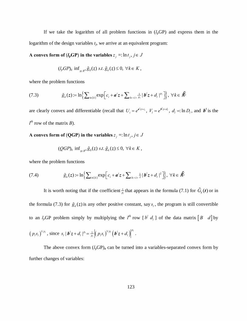
123
If we take the logarithm of all problem functions in (lpGP) and express them in the
logarithm of the design variables tj, we arrive at an equivalent program:
A convex form of (lpGP) in the variables =: ln ,j jz t j J∈
(lpGP)z 0 inf ( ) . . ( ) 0, m kRg s t g k K
∈≤ ∀ ∈% %
zz z ,
where the problem functions
(7.3) { }1[ ]
ˆ( ) : ln exp | | , l
l
pi lk i lpi k l i
g c d k K∈ ∈< >
= + + + ∀ ∈ ∑ ∑z a z b z%
are clearly convex and differentiable (recall that , , : lni l
i lc di l l lU e V e d D+ += = =a z b z , and lb is the
lth row of the matrix B).
A convex form of (QGP) in the variables =: ln ,j jz t j J∈
(QGP)z 0 inf ( ) . . ( ) 0, m kRg s t g k K
∈≤ ∀ ∈% %
zz z ,
where the problem functions
(7.4) { }212[ ]
ˆ( ) : ln exp | | , i lk i li k l i
g c d k K∈ ∈< >
= + + + ∀ ∈ ∑ ∑z a z b z%
It is worth noting that if the coefficient 1lp that appears in the formula (7.1) for ( )kG% t or in
the formula (7.3) for ( )kg% z is any other positive constant, say ls , the program is still convertible
to an lpGP problem simply by multiplying the lth row [ llb d ] of the data matrix [ ]B d by
( )1/ lpl lp s , since ( ) ( )1/1| |
lll
l
pppl ll l l l lps d p s d+ = +b z b z .
The above convex form (lpGP)z can be turned into a variables-separated convex form by
further changes of variables:
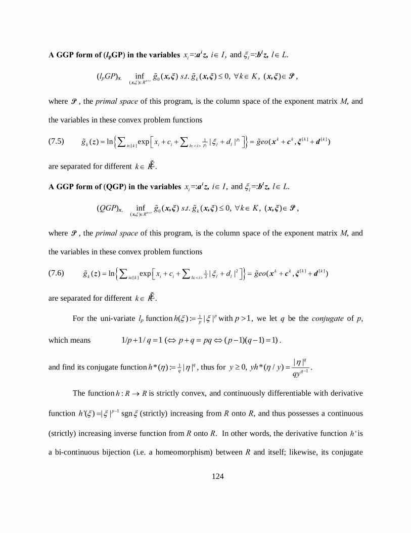
124
A GGP form of (lpGP) in the variables =: , and =: .i lx i I l Lξ∈ ∈i la z, b z,
(lpGP)x,� 0( )
inf ( ) . . ( ) 0, , ( )n r kR
g s t g k K+∈
≤ ∀ ∈ ∈x,
x,ξ x,ξ x,ξ% %ξ
P ,
where P , the primal space of this program, is the column space of the exponent matrix M, and
the variables in these convex problem functions
(7.5) { } [ ] [ ]1[ ]
( ) ln exp | | ( , )l
l
p k k k kk i i l lpi k l i
g x c d geoξ∈ ∈< >
= + + + = + + ∑ ∑z x c ξ d% %
are separated for different ˆk K∈ .
A GGP form of (QGP) in the variables =: , and =: .i lx i I l Lξ∈ ∈i la z, b z,
(QGP)x,� 0( )
inf ( ) . . ( ) 0, , ( )n r kR
g s t g k K+∈
≤ ∀ ∈ ∈x,
x,ξ x,ξ x,ξ% %ξ
P ,
where P , the primal space of this program, is the column space of the exponent matrix M, and
the variables in these convex problem functions
(7.6) { }2 [ ] [ ]12[ ]
( ) ln exp | | ( , )k k k kk i i l li k l i
g x c d geoξ∈ ∈< >
= + + + = + + ∑ ∑z x c ξ d% %
are separated for different ˆk K∈ .
For the uni-variate lp function 1( ) : | |pph ξ ξ= with 1p > , we let q be the conjugate of p,
which means 1/ 1/ 1 ( ( 1)( 1) 1)p q p q pq p q+ = ⇔ + = ⇔ − − = .
and find its conjugate function 1*( ) : | |qqh η η= , thus for 1
| |0, *( / )q
qy yh yqyηη −≥ =
.
The function :h R R→ is strictly convex, and continuously differentiable with derivative
function 1'( ) | | sgnph ξ ξ ξ−= (strictly) increasing from R onto R, and thus possesses a continuous
(strictly) increasing inverse function from R onto R. In other words, the derivative function 'h is
a bi-continuous bijection (i.e. a homeomorphism) between R and itself; likewise, its conjugate

125
function * :h R R→ , being a function of the same type as h with 1q > , and its derivative function
1* '( ) | | sgnqh η η η−= have exactly the same properties mentioned above. This pair of functions h
and h* of course are lsc, proper convex. They satisfy a conjugate inequality:
(7.7) 1 1| | | | , ,p qp q Rξ η ξη ξ η+ ≥ ∀ ∈
where equality holds exactly when one of the following 3 equivalent conditions holds true:
(7.8)
1
1
( ) '( ) | | sgn( ) * '( ) | | sgn( ) | | | |
p
q
p q
a hb hc
η ξ ξ ξξ η η ηξη ξ η
−
−
= =
= =
= =
Since ( ) ( ), ' and *'a b h h⇔ are each other’s inverse functions.
From (5.6) we can derive
Dual program (lpGD) (Convention: 1| | /( ) 0 for 0 and = for 0l lq ql l i i l i lq y y yη η η− = = = ∞ = ≠ )
(7.9) (lpGD)
1ˆ( ) [ ]
0
1
| |sup ( , ) : exp
. . 1, (Normality Condition)
0,
il
ln r
y qi k l
l l qR R l ii kk K i Ii l i
r
ij i lj li l
CV dy q y
s t
a y b j J
λ ηη
λ
η
+−
∈ × ∈< >∈∈ ∈
=
= ⋅ −
=
+ = ∈
∑ ∑∏∏
∑
y,η
% y η
1
[ ]
(Orthogonality Conditions)
ˆ 0, , ,
0 0, , (*)
n
i i ki k
i l
y i I y k K
y l i i I
λ
η
=
∈
+
≥ ∀ ∈ = ∀ ∈
= ⇒ = ∀ ∈< > ∀ ∈
∑
∑
Dual program (QGD) (Convention: 2| | /(2 ) 0 for 0 and = for 0l i i l i ly y yη η η= = = ∞ = ≠ )
(7.10) (QGD)
2
ˆ( ) [ ]
| |sup ( , ) : exp 2
. . exactly the same constraints as in the above (l GD)
i
n r
y
i k ll l
R R l ii kk K i Ii i
p
CV dy y
s t
λ ηη+∈ × ∈< >∈∈ ∈
= ⋅ −
∑ ∑∏∏y,η
% y η

126
7.2 MAIN LEMMA OF lPGP
The main lemma of (lpGP) follows from the main lemma of CGP (Lemma 5.2.1).
Lemma 7.2.1 (Main Lemma of lpGP) If t is feasible for primal program (lpGP) and ( , )y η is
feasible for dual program (lpGD), then 0 ( ) ( , )G V≥% %t y η
Moreover, under the same conditions, 0 ( ) ( , )G V=% %t y η if, and only if, one of the following two
sets of equivalent conditions holds:
(7.11) 1
( ) 1, , ( )
ˆ( ) ( ), [ ],
( ) | ln ( ) | sgn(ln ( ) ), ,
k
l
k
i k k i
pl i l l
G k Ka
y G U i k k K
b y V V l i i I
λ
λ
η − +
= ∈
= ∈ ∈= ∈< > ∈
t
t t
t t
%
% %
(Extremality condition 1)
(7.12) 0
1
( ) ( ), [0] ( )
( ), [ ],
( ) | ln ( ) | sgn(ln ( ) ), , l
ii
k i
pl i l l
U G ic y
U i k k K
d y V V l i i I
λ
η − +
∈= ∈ ∈
= ∈< > ∈
t t
t
t t
%%
%
(Extremality condition 2)
(Condition (b) is equivalent to 1( ) ' ln ( ) sgn | / | , if 0, , lql l l i ib V y y l i i Iη η − += ⋅ > ∀ ∈< > ∈t ) in
which case t is optimal for primal program (lpGP) and ( , )y η is optimal for dual program
(lpGD). (Recall from Lemma 2.1.0 that the above conditions (a) and (c) are equivalent.)
Lemma 7.2.2 (Main Lemma of QGP) If t is feasible for primal program (QGP) and ( , )y η is
feasible for dual program (QGD), then 0 ( ) ( , )G V≥% %t y η
Moreover, under the same conditions, 0 ( ) ( , )G V=% %t y η if and only if one of the following two sets
of equivalent conditions holds:

127
(7.13) ( ) 1, ,
( )ˆ( ) ( ), [ ],
( ) ln ( ) , ,
kk
i k k i
l i l
G k Ka
y G U i k k K
b y V l i i I
λ
λ
η +
= ∈
= ∈ ∈= ∈< > ∈
t
t t
t
%
% %
(Extremality condition 1)
(7.14) 0( ) ( ) , [0]
( ) ( ), [ ],
( ) ln ( ), ,
ii
k i
l i l
U G ic y
U i k k K
d y V l i i I
λ
η +
∈= ∈ ∈
= ∈< > ∈
t tt
t
%%%
(Extremality condition 2)
(Condition (b) is equivalent to ( ) ' ln ( ) / , if 0, , l l i ib V y y l i i Iη += > ∀ ∈< > ∈t ) in which case t is
optimal for primal program (QGP) and ( , )y η is optimal for dual program (QGD). (Recall from
Lemma 2.1.0 that the above conditions (a) and (c) are equivalent.)
Corollary 7.2.3 (Weak Duality Theorem for (lpGP))
3) Always inf sup 0p pl GP l GD∞ ≥ ≥ ≥
4) When (lpGP) and (lpGD) are feasible, inf sup 0.p pl GP l GD∞ > ≥ >
Corollary 7.2.4 (Weak Duality Theorem for (QGP))
5) Always inf sup 0QGP QGD∞ ≥ ≥ ≥
6) When (QGP) and (QGD) are feasible, inf sup 0.QGP QGD∞ > ≥ >
7.3 FIRST AND SECOND DUALITY THEOREMS OF lPGP
The first duality theorem of (lpGP) follows from the First Duality Theorem of CGP (Theorem
5.3.1). The statement for the first duality theorem of (QGP) is almost exactly the same, so it is
not repeated here.

128
Theorem 7.3.1 (First Duality Theorem of lpGP) Suppose that primal program (lpGP) is
superconsistent. Then the following 3 conditions are equivalent:
1) t’ is a minimal solution to (lpGP).
2) There exists a vector ' pR+∈λ for z’ (where z’= ln t’) such that ( ', ')z λ forms a saddle
point of ( , )l z% λ .
3) There exists a vector ' pR+∈λ for z’ (where z’= ln t’) such that ( ', ')z λ satisfies the
KKT conditions for (lpGP)z:
' '
' '0ˆ
( ) 0, ( ) 0, ( ) 0,
( ) ( , ') ( ) , 1k k k k
z k kk K
a g g k K
b l g where
λ λ
λ λ∈
≥ ≤ = ∀ ∈
∇ = ∇ = =∑z' z'
z' z'
% %% % 0λ
in which case the set of all such vectors 'λ is a non-empty compact convex subset of pR+ , and the
dual program (lpGD) also has a maximum solution ( ', ')y η such that
p 0 pmin( GP) ( ') ( ', ') max( GD)l G V l= = =% %t y η (Perfect duality)
A theorem of the alternatives from linear programming duality theory
Of the following two linear systems exactly one has a solution (where : ( )AM n r mB
= + × ):
(I) Find z with 0 0, 0≠ ≤ =Az Bz (II) Find with , and T TA B
> + =y y 0 y 0η η
We say that program (lpGD) is canonical if system (II) has a solution when M is the program’s
composite exponent matrix.
Theorem 7.3.2 (Second Duality Theorem of lpGP) Suppose that primal program (lpGP) is
consistent. Then the minimum set of program (lpGP)z is non-empty and bounded if and only if its
dual program (lpGD) is canonical.

129
Proof By assumption, program (lpGP)z is consistent. For the function 1( ) | | with 1pph pξ ξ= > ,
one has 1 10( ) lim | | ( )p p
psh s iξ ξ ξ∞ −
→∞= = . Thus
[ ]0[ ]
( ) max ( ) max( ) ( )k kk l ii k
g i i∞∈< >∈
= + = + ∑i l0z a z b z A z B z%
and system (5.19) becomes
[ ]ˆ ˆ( ) 0, max( ) 0, ,
,
k kkg k K k K∞ ≤ ∀ ∈ ⇔ ≤ = ∀ ∈
⇔ ≤ =
z A z B z 0Az 0 Bz 0
%
Since M is of full column rank, it is one-to-one, hence 0 0≠ ⇒ ≠z Mz . Therefore by theorem
2.5.10,
The minimum set of program (lpGP)z is non-empty and bounded
⇔ The system ˆ( ) 0, kg k K∞ ≤ ∈z% has no non-trivial solution in z
⇔ System (I) above has no solution
⇔ System (II) above has a solution, i.e. program (lpGD) is canonical ∎
Theorem 7.3.3 (Second Duality Theorem of QGP) Suppose that primal program (QGP) is
consistent. Then the minimum set of program (QGP)z is non-empty and bounded if and only if its
dual program (QGD) is canonical.

130
8.0 CONCLUSION AND SOME DIRECTIONS OF FUTURE RESEARCH
In this chapter we summarize the contributions of this research and suggest some directions for
future work.
8.1 SUMMARY OF CONTRIBUTIONS
In this thesis, the traditional GP models have been extended to the more general
Exponential GP models, and then to the even more general Composite GP models. The latter
generalization includes (QGP), (lpGP) and (EGP) as important special cases. It was also shown
that all of these are special cases of Peterson’s GGP models, for which only a Main Lemma is
available, and First and Second duality theorem are not defined or proved.
For the Main Lemma, multiple direct proofs have been provided, with a second set of
equivalent Extremality Conditions in each extended case.
For the First duality theorem, it was shown that a superconsistent primal program (CGP)
has a minimal solution 't if, and only if, there exists a vector ' pR+∈λ such that ( ', ')z λ forms a
saddle point of the Lagrangian ( , )l z% λ and if, and only if, it satisfies the KKT conditions for
(CGP)z. It was also shown that in this case the set of all such Lagrange multiplier vectors λ is a

131
non-empty compact convex subset of pR+ , whereas the original theorem is a “If…then” statement
and merely showed the existence of λ for the (GP) case.
For the Second duality theorem, it was shown that for the important special cases of
(QGP), (lpGP) and (EGP), the minimum set of a consistent primal program is non-empty and
bounded if, and only if, its dual program is canonical, whereas the original theorem merely
showed the existence of a primal solution for the (GP) case, when its dual program is canonical.
For the Sensitivity Analysis of the extended GP model, it was shown that for an optimal
solution *z of (CGP)z, the following constitiute the sensitivity information:
* * ** * *0 0 0
* ** * * *0 0
( ) ( ) ( ), , ,
( ) ( ), , where ln
i l ki l k
i j l j k kij lj
g g gyc d b
g gy z z b Ba b
η λ
η
∂ ∂ ∂= = = −
∂ ∂ ∂
∂ ∂= = =
∂ ∂
% % %
% %
z z z
z z,
where kB is the new right hand side replacing 1 for the kth constraint in (CGP).
A computational procedure for the ‘Dual to primal conversion’ of optimal solutions,
when there is no duality gap, i.e. 0( ) ( , )G V= y% %t η was also derived.
8.2 SOME DIRECTIONS FOR FUTURE RESEARCH
The first extension would be to prove a strong version of the First Duality Theorem of
(CGP): If a primal program (CGP) is superconsistent and has a finite infimum, then the dual
program (CGD) has a maximum solution ( ', ')y η such that inf(CGP) max(CGD) ( ', ')V= = % y η .

132
Following this one could explore the Second duality theorem: The minimum set of a
consistent primal program is non-empty and bounded if and only if its dual program is
canonical, to see if it holds for other branches of CGP. So far, it is only shown to hold for
(EGP), (QGP), and (lpGP). On the other hand, it might be possible to show for the last three
cases that, if the dual program is canonical and has a finite positive supremum, then a primal
minimum solution exists and there is no duality gap.
Finally, it is worth searching for more examples of practical applications of (CGP), and
developing computational algorithms exploiting the duality theory.

133
APPENDIX A
MATHEMATICAL PROOFS OF SOME INEQUALITIES
Geometric Programming duality hinges upon a so-called geometric inequality, which is a slight
generalization of the classical (weighted) arithmetic-geometric mean (AGM) inequality, whose
strict version is equivalent to the strict convexity of the exponential function exp x and to the
strict concavity of the logarithmic function ln x.
A.1 ON STRICTLY CONVEX FUNCTIONS
We say a real-valued function f on a non-empty convex set nC R⊂ is strictly convex on C if
, (0,1), [(1 ) ] (1 ) ( ) ( )x y C t f t x ty t f x tf y∀ ≠ ∈ ∀ ∈ − + < − + , (Rockafellar, 1970, p.253). A
function g is strictly concave on C, if –g is strictly convex on C (i.e. if the above defining
inequality holds in reverse direction). Strict convexity is essentially a 1-dimensional property;
behavior with respect to line segments is all that matters. A function f is strictly convex if and
only if (iff) it is strictly convex relative to every line.
Proposition 1 A real-valued function f on a non-empty convex set C is strictly convex on C iff
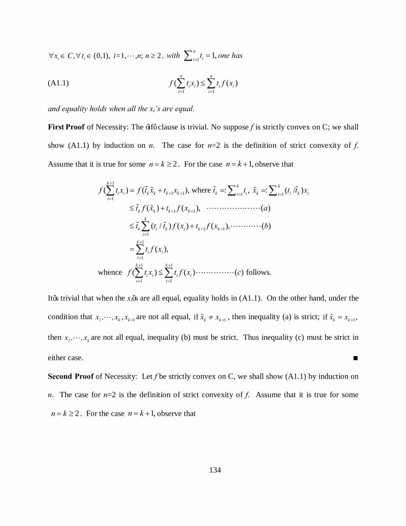
134
, (0,1), =1, , ; 2i ix C t i n n∀ ∈ ∀ ∈ ≥L , with1
1,nii
t=
=∑ one has
(A1.1) 1 1
( ) ( )n n
i i i ii i
f t x t f x= =
≤∑ ∑
and equality holds when all the xi’s are equal.
First Proof of Necessity: The ‘if’ clause is trivial. No suppose f is strictly convex on C; we shall
show (A1.1) by induction on n. The case for n=2 is the definition of strict convexity of f.
Assume that it is true for some 2n k= ≥ . For the case 1,n k= + observe that
1
1 1 1 11
1 1
1 11
( ) ( ), where : , : ( / )
( ) ( ), ( )
( / ) ( ) ( ), ( )
k k ki i k k k k k i k i k ii i
i
k k k k
k
k i k i k ki
i
f t x f t x t x t t x t t x
t f x t f x a
t t t f x t f x b
t
+
+ + = ==
+ +
+ +=
= + = =
≤ +
≤ +
=
∑ ∑ ∑
∑
% % %% %
% % LLLLLLL
% % LLLL
1
11 1
1 1
( ),
whence ( ) ( ) ( ) follows.
k
ii
k k
i i i ii i
f x
f t x t f x c
+
=
+ +
= =
≤
∑
∑ ∑ LLLLL
It’s trivial that when the xi’s are all equal, equality holds in (A1.1). On the other hand, under the
condition that 1 ,1 k kx , ,x x +L are not all equal, 1if k kx x +≠% , then inequality (a) is strict; 1if ,k kx x +=%
then 1 kx , ,xL are not all equal, inequality (b) must be strict. Thus inequality (c) must be strict in
either case. ∎
Second Proof of Necessity: Let f be strictly convex on C, we shall show (A1.1) by induction on
n. The case for n=2 is the definition of strict convexity of f. Assume that it is true for some
2n k= ≥ . For the case 1,n k= + observe that

135
1 1
1 1 11 1
1
1 11
( ) ( ), where : , : ( ) /
( ) ( ), with equality holding iff ... =
( ) [( ) ( ) (k
k
k k
i i i i k k k k k k k k k k ki i
k
i i k k k ki
t ti i k ks
f t x f t x s y s t t y t x t x s
t f x s f y x x y
t f x s f x
+ −
+ + += =
−
−=
= + = + = +
≤ + = =
≤ + +
∑ ∑
∑
11
1 11
1
1
) ( )], with equality holding iff
( ),
k
k
k
k k ksi
k
i ii
f x x x
t f x
+
−
+ +=
+
=
=
=
∑
∑
1 1
1 11 1
whence ( ) ( ) follows, and equality holds iff ... = .k k
i i i i k ki i
f t x t f x x x x+ +
+= =
≤ = =∑ ∑
1 1 1 1 1 1(since ... = , and ... = )k k k k k k kx x y x x x x x x− + − += = = ⇔ = = = ∎
If we relax the weight requirements in the above proposition from 0it > to 0iδ ≥ , then
the strict convexity of f can be rephrased as follows. A real-valued function f defined on a non-
empty convex set nC R⊂ is strictly convex iff , 0, 1, , ,i ix C i nδ∀ ∈ ∀ ≥ = L with1
1,nii
δ=
=∑
where 2 n N≤ ∈ , one has
1 1( ) ( ),
n n
i i i ii i
f x f xδ δ= =
≤∑ ∑
and equality holds exactly when all the xi’s for which 0iδ > are equal. Geometrically, this
implies that if { }1,1 : co , ,n
i i nix x x xδ
== ∈ …∑ the convex hull of a set of n distinct points 1, , nx x… ,
but x is not any of the generating points 1, , nx x… , then x is in the convex hull of a set of at least
two distinct points among 1, , nx x… , and 1
( ) ( )n
i ii
f x f xδ=
< ∑ [Duffin et.al. 1967, p. 56, exercise
2(a)].
It is easy to identify strictly convex functions when they are also differentiable
[Rockafellar and Wets, 2004, p.46].

136
Theorem 2 (1-dimensional derivative tests). For a differentiable function f on an open interval
I R⊂ , each of the following conditions is equivalent to f being strictly convex on I:
(a) f′ is increasing on I: any points 0 1x x< in I satisfy 0 1 ' ( ) '( ).f x f x<
(b) ( ) ( ) '( )( ), , with .f y f x f x y x x y I x y− > − ∀ ∈ ≠
The following condition is only sufficient, but not necessary for f being strictly convex (The
strictly convex function f(x) =x4, on R with ''(0) 0f = serves as a counter-example.)
(c) ''( ) 0, f x x I> ∀ ∈ (Assuming twice differentiability).
Example 1
• ( ) axf x e= is strictly convex on R when 0.a ≠
• ( ) ln( )f x bx= is strictly concave on (0,∞) when 0.b >
• strictly convex, if 1 0. (e.g. , 1 / )
( ) on (0, ) is strictly concave, if 0 1. (e.g. )
r r or r x x xf x x
r x
> <= ∞ < <
Solution. Since 1 ( 1)ln increasing on (0, ), if 1 0.'( ) is
decreasing on (0, ), if 0 1.r r x r or r
f x rx rer
− − ∞ > <= = ∞ < <
∎
Example 2 [Duffin et.al. 1967, p. 56, exercise 2(b)]
, , ,x y z R∀ ∈2 2 21 1 1
2 3 6 2 3 6ln( )y x y zx z e e e+ + < + + , unless x=y=z.
Solution Since the function2
( ) : tf t e= has second derivative2 2''( ) 2 (1 2 ) 0, ,tf t e t t= + > ∀ it is
strictly convex; hence , , ,x y z R∀ ∈2 2 22 1 1 1
2 3 6 2 3 6 exp( )y x y zx z e e e+ + < + + , unless x=y=z; i.e.
2 2 21 1 1
2 3 6 2 3 6 ln( )y x y zx z e e e+ + < + + , unless x=y=z. ∎

137
For any two functions f and g we define their maximum and minimum as follows:
( )( ) : max[ ( ), ( )], ( )( ) : min[ ( ), ( )]f g x f x g x f g x f x g x∨ = ∧ =
Theorem 3 If f and g are strictly convex, so is f ∨g.
A.2 THE AGM INEQUALITY AND THE GEOMETRIC INEQUALITY
The classical inequality relating the arithmetic mean to the geometric is stated and proved in any
book on inequalities, e.g. [Beckenbach and Bellman, 1965], and [Hardy, Littlewood, and Polya,
1952, pp.17-18]. We show below that the strict version of this classical (weighted) AGM
inequality is actually equivalent to the strict convexity of the exponential function exp x and to
the strict concavity of the logarithmic function ln x.
Theorem 3 (Strict AGM Inequality)
10, 0, , with , where 2 ,n
i i iiT i = 1, ,n n Nδ δ λ
=∀ > ∀ > = ≤ ∈∑L
1 1
i
nn
i i ii i
T Tλ
δ λδ λ= =
≥ ⋅ ∑ ∏ ,
where equality holds exactly when all the Ti’s are equal. When 1λ = , this reduces to the more
familiar equivalent form [Duffin and Peterson 1966, p.1316, Lemma 0]:
1 1
i
nn
i i ii i
T T δδ= =
≥∑ ∏ ,
where equality holds exactly when all the Ti’s are equal.
Proof The convexity of the exponential function xe applied to the points lni ix T= with weights
/i it δ λ= means:

138
1 1
/
1 11 1
1 1 exp( ln ) exp(ln )
1 i i
n n
i i i ii i
n nn n
i i i i i ii ii i
T T
T T T Tλ
δ λ δ λ
δ δλ λ
δ λ δλ
= =
= == =
≤
⇔ ≤ ⇔ ⋅ ≤
∑ ∑
∑ ∑∏ ∏.
The concavity of the logarithmic function ln x applied to the points i ix T= with weights /i it δ λ=
means:
1 1
/
1 11 1
1 1
1i i
n n
i i i ii i
n nn n
i i i i i ii ii i
ln T lnT
T T T Tλ
δ λ δ λ
δ δλ λ
δ δ λλ
= =
= == =
≥
⇔ ≥ ⇔ ≥ ⋅
∑ ∑
∑ ∑∏ ∏
The condition for equality in both cases is the same: all the Ti’s are equal. ∎
Remark If the assumption 0iT > in the above theorem is relaxed to 0iT ≥ , the conclusion still
holds. Furthermore, one can also relax the assumption 0iδ > to 0iδ ≥ and obtain:
Theorem 4 (Relaxed AGM Inequality)
10, 0, , 2n
i i iiT i = 1, ,n, with where n Nδ δ λ
=∀ ≥ ∀ ≥ = ≤ ∈∑L
1 1
i
nn
i i ii i
T Tλ
δ λδ λ= =
≥ ⋅ ∑ ∏ ,
where equality holds exactly when all the Ti’s for which 0iδ > are equal. For 1λ = , this reduces
to the more familiar form:
1 1
i
nn
i i ii i
T T δδ= =
≥∑ ∏

139
Convention: Since 0lim 1,aa a↓ = we define 00 1= , and thus 0 0( / 0) 1, for 0u u u= = ≥ .
Proof: (Case 1) When 0,λ = { }0, : 1,..., ,i i I nδ = ∀ ∈ = and the inequality holds trivially as “1=1”,
and the condition for equality also holds trivially since there is no positive iδ .
(Case 2) When 0,λ > by applying Theorem 3 and the above remark to the index set
{ } : 0iI i I δ+ = ∈ > ≠ φ , one obtains
1 1
i i
nn
i i i i i ii ii I i I
T T T Tλλ
δ δλ λδ δ λ λ+ += =∈ ∈
= ≥ ⋅ = ⋅
∑ ∑ ∏ ∏
Thus the desired inequality follows. The condition for equality is: all the Ti’s for which
(i.e., 0)ii I δ+∈ > are equal. ∎
We can slightly generalize the above weighted AGM Inequality to obtain the following
Theorem 5 (Geometric Inequality)
0, 0, =1, , ,i iU i nδ∀ ≥ ∀ ≥ L with1 1
, ,n ni ii i
U G δ λ= =
= =∑ ∑ one has
1 1
( ) ( ) inn
i i ii iU U δλ λλ δ
= =≥ ⋅∑ ∏
where equality holds iff = , 1, ,i iU G i nλ δ ∀ = L ,i.e., iff 's and 's i iU δ are in proportion.
When 1λ = , this becomes
1 1( ) .i
nni i ii i
U U δδ= =
≥∑ ∏
Note: The original version in [Duffin and Peterson 1966, p.1316, Lemma 1] requires 0,iU i> ∀ .
Proof: (Case 1) When 0,λ = { }0, : 1,..., ,i i I nδ = ∀ ∈ = and the inequality holds trivially as “1=1”,
and the condition for equality also holds trivially as “0=0”.
(Case 2) When 0,λ > define { } : 0iI i I δ+ = ∈ > ≠ φ , and : ,i i iT U i Iδ += ∀ ∈ . Observe that

140
, by (1.16),
= ( ) ( )
i
i i
i i i i ii I i I i I i I
i i i ii Ii I
U U T T
U U
λ λλδ λ
δ δλ λ
δ λ
δ λ δ λ
+ + +
+
∈ ∈ ∈ ∈
∈∈
≥ = ≥ ⋅
⋅ = ⋅
∑ ∑ ∑ ∏
∏ ∏
Hence, one has ( ) ii i i
i I i I
U Uλ
δ λδ λ∈ ∈
≥ ⋅ ∑ ∏ and this is an equality iff
=0, = , = , , since >0.
, i i i
i ii
U i I U T i IT U G i I
G TT T T i Iδ
λ δ λλ
+
+
∀ ∉ ∀ ∈ ⇔ ∃ → ⇔ ∀ ∈ =∃ → = ∀ ∈
∎

141
APPENDIX B
THE STIMULANT OF THE BIRTH OF GP – ZENER’S DISCOVERY
The root of GP lies in some rudimentary work by Zener (1961) for optimizing a posynomial. He
first observed the following fact.
Lemma 1 Let t* be a local minimum (or local maximum) point of the posynomial ( )G t . Then the
following linear system
(B1.1) 1
1
0, 1, , (Orthogonality conditions)
1, (Normality condition)
n
ij ii
n
ii
a j mδ
δ
=
=
= ∀ = =
∑
∑
L
has a positive solution, namely, *δ defined by
(B1.2) * * *: ( ) / ( ), i iU t G t iδ = ∀ .
Together, t* and *δ satisfy:
(B1.3) *
* * **
1
( ) ( ), where ( ) :in
i
i i
CG t V Vδ
δ δδ=
= =
∏
and
(B1.4) * * *
*
1
( ) ( )( ) ( ), i=1, , . (dual-to-primal converson)m
i iij j
j i i
U t Va lnt ln ln nC C
δ δ=
= = ∀∑ L

142
Proof 1) The orthogonality condition is simply a necessary condition for local optimality of
*( )G t at * t (It is in fact also a sufficient condition for global minimality, since optimizing a
posynomial ( )G t amounts to optimizing a certain convex function ( )g z ):
* ** **
* *1 1
( )( ) ( ) 0 0 0, by (1.1.5) 0, 1, , ,( ) ( )
n nj ij i
ij ii ij j
t a U tG t G t a j mt t G t G t
δ= =
∂ ∂= ⇒ ⋅ = ⇒ = ⇒ = ∀ =
∂ ∂ ∑ ∑ L
It can be written more compactly in matrix form as * 0tA δ = , and geometrically, this means the
vector *δ is orthogonal to all the columns of the matrix A. The normality condition is obvious
from the definition of *δ . This proves (B1.1).
2) (B1.3) follows from (B1.1):
* *
***
1
*** * * * *
* *1 1 1 1 1 1
( )( ) [ ( )] ( ) ( ) ( ) ( )
ni i
ij iiiji i
n n n n m m aai i
j ji i i i j ji i
U t CG t G t t V t Vδ
δ δδ
δ δ δδ δ
=
= = = = = =
∑ = = = ⋅ = ⋅ =
∏ ∏ ∏ ∏ ∏ ∏
3) (B1.4) follows from the definitions of * * ( ), i iU t δ and (B1.3). ∎
In essence, Zener discovered that at an optimizing point t* for ( )G t , the vector δ*
defined in Theorem 1 is a positive solution to system (B1.1) and together with t*, satisfy (B1.3)
and (B1.4). Conversely, a positive solution to (1) does not necessarily satisfy (0) for any given
t*, and hence does not necessarily satisfy (2) and (3). A later duality result (Main Lemma for
Unconstrained GP) by Duffin showed that for a positive vector t*, and a nonnegative solution δ*
to (1), (0) and (2) are actually equivalent. However, when n=m+1 and the linear system (1) is
non-singular, it has a unique solution, and if it happens to be positive, it must be the solution
defined by (0), and hence must satisfy (2) and (3). Thus Zener found the optimum value ( *)G t
may be expressed by a simple formula (2) in this special case n-m-1=0, and the optimizing point
t* may also be calculated by solving another system of linear equations (3), whose solution is

143
unique iff A has full column rank (this is certainly the case if the system (1) is non-singular). In
GP literature the number, n-m-1, is called the degree of difficulty of the GP problem.
There is one linear relation among the equations in (3), though. To see this, we first write
(3) in matrix form Az=b*, where A=(aij), lnj jz t= , ( )* *: ln / *i i ib C vδ= + , and v*=: *ln ( )V δ , then
any solution δ* given by (1) satisfies
* * * * * * *1 1
0 0, and ln( / ) ( ) * * * 0.n nti i i ii i
Az A z z b C v v vδ δ δ δ δ δ= =
⋅ = ⋅ = ⋅ = ⋅ = + = − + =∑ ∑Thus * *( ) 0,Az bδ ⋅ − = for a nonzero δ*,which means at least one linear equation is a
consequence of the remaining linear equations.
Remarkably, the optimum value G(t*) was found in (2) before the optimizing point t*
was determined in (3) (On one rare occasion when n=2, m=1, however, this order can be
reversed, as we see in Chapter 2.) It is also obvious that in this case the relative contribution *iδ
of each term does not depend on the cost coefficients Ci, since δ* is uniquely determined by the
matrix A alone.
Let’s illustrate Zener’s procedure with a three-term two-variable unconstrained GP:
Example 1 0 1 2 3inf ( ) ( ) ( ),t U t U t U t> + + where 1 21 2( ) , i=1,2,3.i ia a
i iU t C t t=
1) In the following, define 1 2 3, ,D D D , where ( , )D ⋅ ⋅ denotes the determinant function of row
vectors,
21 31 31 112 3 3 11 21 31 2 11 31
22 32 32 1222 32 12 32
1 1 1 1 1 1
0 ( , ), 0 ( , ),
0 0
a a a aD a a D a a D a a D a a
a a a aa a a a
= = = = = =
11 21 1 23 11 21 11 21 31 1 2 3
12 2212 22 12 22 32
1 1 1 1 1 1
0 ( , ),
0
a aD a a D a a D a a a D D D
a aa a a a a
= = = = = + +

144
We assume that all Di>0 orall Di<0 so that, by Cramer’s rule, the following system
1 2 3
11 1 21 2 31 3
12 1 22 2 32 3
1 0
0a a aa a a
δ δ δδ δ δδ δ δ
+ + = + + = + + =
has a unique solution * 1 2 3( , , ) 0D D DD
δ = >
2) Compute the dual function value *( )V δ which equals the minimum value * ( )G t
*3 3 3
* * * **
1 1 1
: ( ) ( ) : :
DD iii DD
i
i i iD
i i iDi i
C C CG G t V D VD
δ
δδ= = =
= = = = = =
∏ ∏ ∏
Calculate * * * * / , and : ln( / ), 1,2,3.i i i i iU DV D x U C i= = ∀ =
3) * * *
11 1 12 2 1
* * *21 1 22 2 2
z + zSolve
z + z
a a xa a x
=
=
to get ( )* *1 12 11 1* * * * * *
1 2 22 1 12 2 11 2 21 1* *3 32 22 21 2
1 1( , ) , ,
x a a xz z a x a x a x a x
D Dx a a x
= = − −
and3 322 12 21 11
* * * *22 1 12 2 3 11 2 21 1 3
1/ 1/* * * *
( )/ ( )/* * 1 2 1 21 2
1 2 1 2
( , ) ( , ) ,
D Da a a aa x a x D a x a x D U U U Ut t e e
C C C C
− −
− − = =
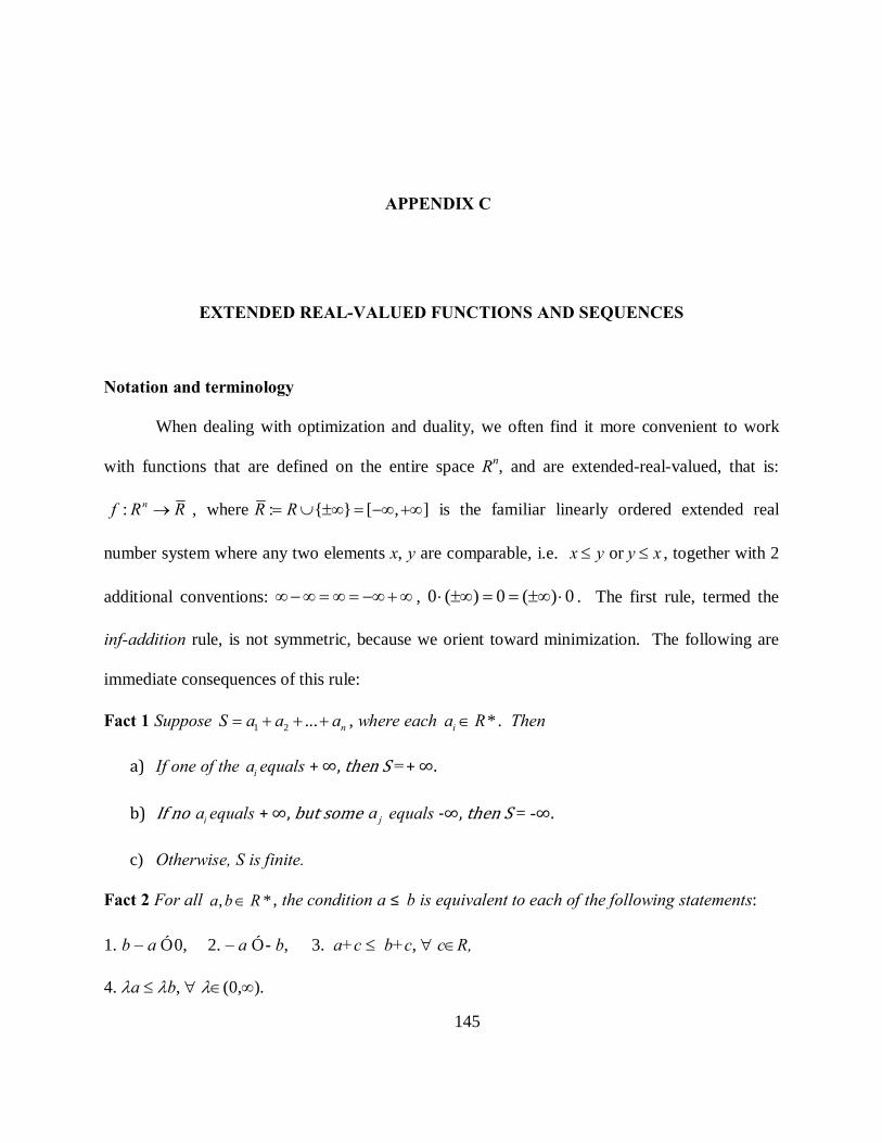
145
APPENDIX C
EXTENDED REAL-VALUED FUNCTIONS AND SEQUENCES
Notation and terminology
When dealing with optimization and duality, we often find it more convenient to work
with functions that are defined on the entire space Rn, and are extended-real-valued, that is:
: nf R R→ , where : { } [ , ]R R= ∪ ±∞ = −∞ +∞ is the familiar linearly ordered extended real
number system where any two elements x, y are comparable, i.e. or x y y x≤ ≤ , together with 2
additional conventions: ∞ − ∞ = ∞ = −∞ + ∞ , 0 ( ) 0 ( ) 0⋅ ±∞ = = ±∞ ⋅ . The first rule, termed the
inf-addition rule, is not symmetric, because we orient toward minimization. The following are
immediate consequences of this rule:
Fact 1 Suppose 1 2 ... nS a a a= + + + , where each *ia R∈ . Then
a) If one of the ia equals + ∞,then S =+ ∞.
b) If no ia equals + ∞,but some ja equals -∞, then S = -∞.
c) Otherwise, S is finite.
Fact 2 For all , *a b R∈ , the condition a ≤ b is equivalent to each of the following statements:
1. b – a ≥ 0, 2. – a ≥ - b, 3. a+c ≤ b+c, ∀ c∈R,
4. λa ≤ λb, ∀ λ∈(0,∞).

146
Note that for c= ± ∞, c - c is not 0, but equals + ∞.

147
Max and Min
A number a in R* is said to be a lower bound for a subset C in R*, if
, a x x C≤ ∀ ∈ . The infimum of C is the greatest lower bound (glb) for C. By this definition,
−∞ is a lower bound for any subset C in R*, and any number a in R* is a lower bound for the
empty set φ, so inf φ = +∞.
Fact 3 For any subset C of R*,
inf( \{ }) inf inf( { })C C C∞ = = ∪ ∞ .
We say that a set C in R* is bounded below if it has a finite lower bound. For example, C is not
bounded below if C− ∞ ∈ . The set C is bounded if it is both bounded below and above.
Fact 4 For any subset C of R*,
a) inf { }C iff C= ∞ ⊂ ∞ b) inf C = −∞ iff C is not bounded below
c) inf C is finite iff C is bounded below and C∩R≠∞.
For any function : *nf R R→ and any subset A of R*, the effective domain of f is
{ }dom : | ( )nF f x R f x= = ∈ < ∞ , the infimum of f over A is =inf : inf ( )A f f Aα = , and the
minimum set of f over A is { } arg min : | ( )Af x A F f x α= ∈ ∩ = . By Fact 3 above, we have
Fact 5 For any function : *nf R R→ and any subset A of R*,
{ } inf inf ( ) inf ( ) | , ( )A f f A F f x x A f x= ∩ = ∈ < ∞ .
We say that a function f is bounded below on a set A if its image set f (A) is bounded below. For
example, f is not bounded below on A if ( )f x = −∞ for some x in A. The function f is bounded
on A if its image set f (A) is bounded. By Fact 4 above, we have
Fact 6 For any function : *nf R R→ and any subset A of *,R
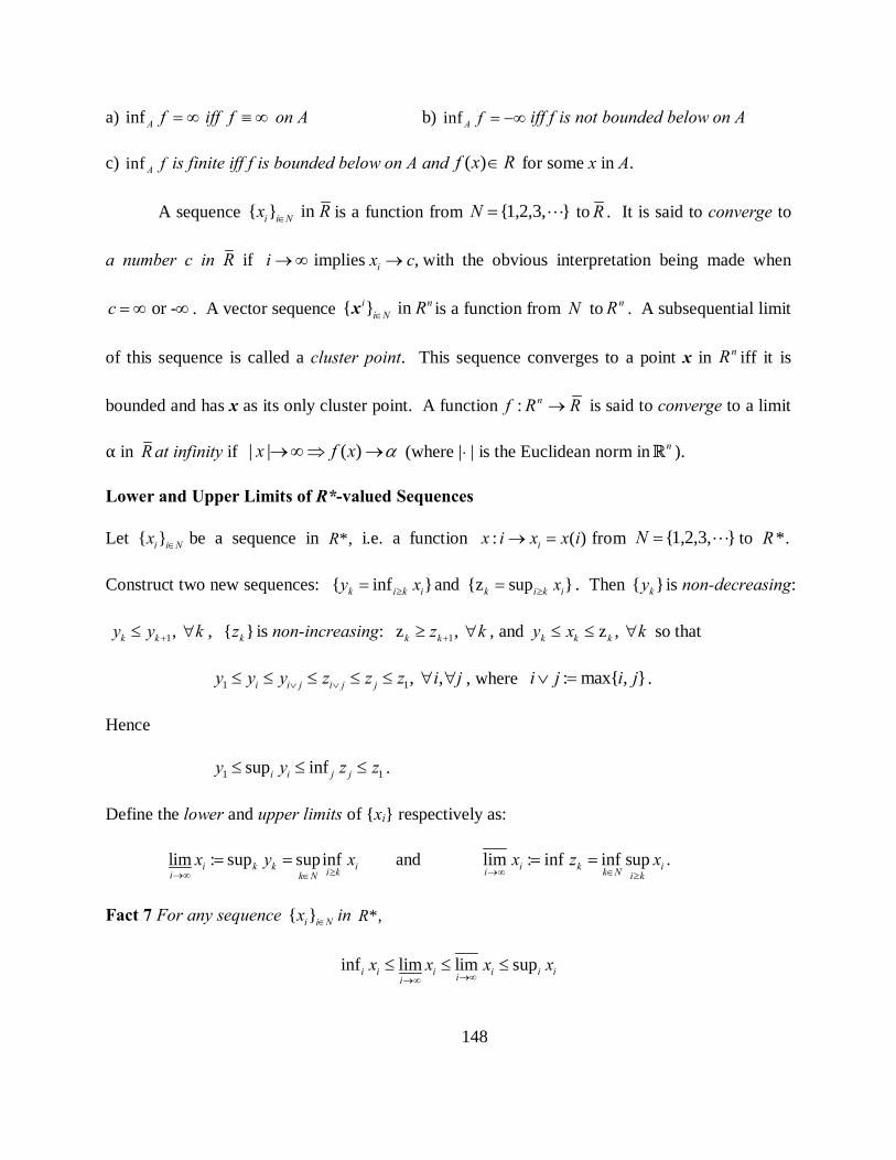
148
a) inf A f iff f= ∞ ≡ ∞ on A b) inf A f = −∞ iff f is not bounded below on A
c) inf A f is finite iff f is bounded below on A and ( )f x R∈ for some x in A.
A sequence { } in i i Nx R∈ is a function from {1,2,3, }N = L to R . It is said to converge to
a number c in R if implies ,ii x c→ ∞ → with the obvious interpretation being made when
or -c = ∞ ∞ . A vector sequence { } in i ni N R∈x is a function from N to nR . A subsequential limit
of this sequence is called a cluster point. This sequence converges to a point x in nR iff it is
bounded and has x as its only cluster point. A function : nf R R→ is said to converge to a limit
α in R at infinity if | | ( )x f x α→ ∞ ⇒ → (where | ⋅ | is the Euclidean norm in nR ).
Lower and Upper Limits of R*-valued Sequences
Let { }i i Nx ∈ be a sequence in *,R i.e. a function : ( )ix i x x i→ = from {1,2,3, }N = L to *.R
Construct two new sequences: { inf }k i k iy x≥= and {z sup }k i k ix≥= . Then { }ky is non-decreasing:
1 , k ky y k+≤ ∀ , { }kz is non-increasing: 1 z , k kz k+≥ ∀ , and z , k k ky x k≤ ≤ ∀ so that
1 1, ,i i j i j jy y y z z z i j∨ ∨≤ ≤ ≤ ≤ ≤ ∀ ∀ , where : max{ , }i j i j∨ = .
Hence
1 1sup infi i j jy y z z≤ ≤ ≤ .
Define the lower and upper limits of {xi} respectively as:
lim : sup supinfi k k ii ki k Nx y x
≥→∞ ∈= = and lim : inf inf supi k ii k N i k
x z x→∞ ∈ ≥
= = .
Fact 7 For any sequence { }i i Nx ∈ in *,R
inf lim lim supi i i i i iiix x x x
→∞→∞≤ ≤ ≤
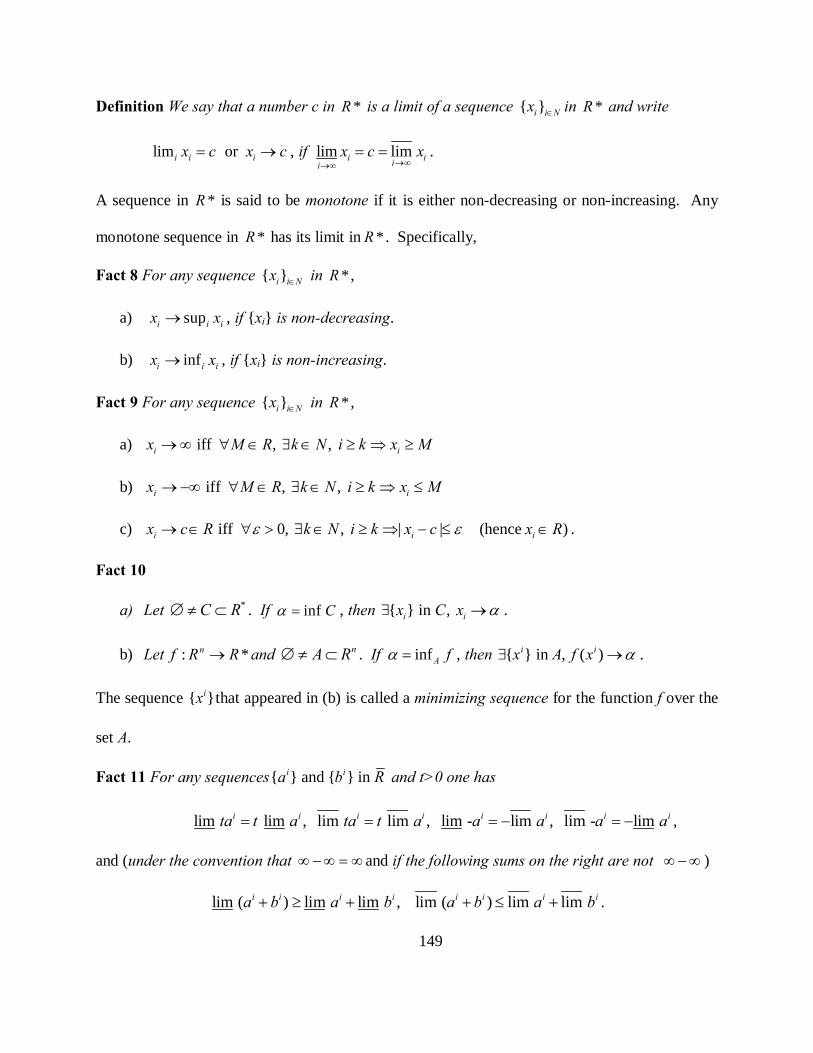
149
Definition We say that a number c in *R is a limit of a sequence { }i i Nx ∈ in *R and write
lim or i i ix c x c= → , if lim lim i iiix c x
→∞→∞= = .
A sequence in *R is said to be monotone if it is either non-decreasing or non-increasing. Any
monotone sequence in *R has its limit in *R . Specifically,
Fact 8 For any sequence { }i i Nx ∈ in *R ,
a) supi i ix x→ , if {xi} is non-decreasing.
b) infi i ix x→ , if {xi} is non-increasing.
Fact 9 For any sequence { }i i Nx ∈ in *R ,
a) iff , , i ix M R k N i k x M→ ∞ ∀ ∈ ∃ ∈ ≥ ⇒ ≥
b) iff , , i ix M R k N i k x M→ −∞ ∀ ∈ ∃ ∈ ≥ ⇒ ≤
c) iff 0, , | | (hence )i i ix c R k N i k x c x Rε ε→ ∈ ∀ > ∃ ∈ ≥ ⇒ − ≤ ∈ .
Fact 10
a) Let * C R∅ ≠ ⊂ . If inf Cα = , then { } in , i ix C x α∃ → .
b) Let : *nf R R→ and nA R∅ ≠ ⊂ . If infA fα = , then { } in , ( )i ix A f x α∃ → .
The sequence { }ix that appeared in (b) is called a minimizing sequence for the function f over the
set A.
Fact 11 For any sequences{ } and { } in i ia b R and t>0 one has
lim lim , lim lim , lim - lim , lim - lim i i i i i i i ita t a ta t a a a a a= = = − = − ,
and (under the convention that ∞ − ∞ = ∞ and if the following sums on the right are not ∞ − ∞ )
lim ( ) lim lim , lim ( ) lim lim i i i i i i i ia b a b a b a b+ ≥ + + ≤ + .

150
Fact 12 For any sequence { } in ii Na R∈ the set of all of its cluster points,
( ) Lim a : { | a subsequence a }ikRα α= ∈ ∃ → , is a closed set in R with ( ) lim min Lim aia = ,
and ( ) lim max Lim aia = . Moreover, ia Rα→ ∈ if and only if Lim (a) = {α}, in which case
lim lim i ia a α= = .

151
BIBLIOGRAPHY
1. Abrams, R.A. [1975], Projections of Convex Programs with Unattained Infima SIAM J. Control, Vol. 13, 3, pp. 706-718.
2. ---[1976], Consistency, Super-consistency, and Dual Degeneracy in Posynomial Geometric Programming, Operations Research, Vol. 24, No. 2, pp.325-335.
3. Avriel, M. (Ed) [1980], Advances in Geometric Programming, Plenum Press, New York and London.
4. Avriel, M., Rijckaert, M.J. and Wilde, D.J. (Eds.) [1973], Optimization and Design, The Impact of Optimization Theory on Engineering Design, Prentice Hall, Englewood Cliffs, New Jersey, pp.3-6.
5. Beckenbach, E.F. and Bellman R.[1965], Inequalities, 2nd revised printing, Springer-Verlag.
6. Beightler, C. S. and Phillips, D. T. [1976], Applied Geometric Programming, John Wiley, New York.
7. Ben-Tal and A. Nemirovski [2001], Lectures on Modern Convex Optimization: Analysis, Algorithms, and Engineering Applications, xii, MPS/SIAM Series on Optimization.
8. Berberian, S.K. [1999], Fundamentals of Real Analysis, Springer-Verlag New York, Inc.
9. Berkovitz, L.D. [2002], Convexity and Optimization in Rn, John Wiley & Sons, Inc., New York, NY.
10. Bertsekas, D.P. [2009], Convex Optimization Theory, Athena Scientific.
11. Bertsekas, D.P., Nedic, A., Ozdaglar, A.E. [2003], Convex Analysis and Optimization, Athena Scientific.
12. Borwein, J.M., and Lewis, A.S. [2006], Convex Analysis and Nonlinear Optimization, 2e, Canadian Mathematical Society.
13. Boyd and Vandenberghe [2004], Convex Optimization, Cambridge University Press.

152
14. Boyd, S., Kim, S.-J., Vandenberghe, L., and Hassibi, A. [2007], A tutorial on geometric programming, Optimization and Engineering, Vol. 8, No.1/March, pp. 67-127. http://www.springerlink.com/content/9941458381562w82/
15. Bronshtein, I.N.; Semendyayev, K.A.; Musiol, G.; Muehling, H. [2004], Handbook of Mathematics, 4th edition, Springer – Verlag. (p.623-624)
16. Chiang, M [2005]. Geometric programming for communication systems, Foundations and Trends in Communications and Information Theory, vol. 2, no. 1-2, pp. 1-154.
17. Colding, B.N. and Konig, W. [1971], Validity of the Taylor Equation in Metal Cutting, Annals of the CIRP, Vol.19, pp.793-812.
18. Colding, B.N. [1959], A 3-dimensional Tool-Life Equation-Machining Economics, Transactions ASME, B 81, pp.239-250.
19. Colding, B.N. [1969], Machining Economics and Industrial Data Manuals, Annals of the CIRP, Vol.17, pp.279-288.
20. Cover, T.M., and Thomas, J., Elements of Information Theory, New York, Wiley, 1991.
21. Dantzig, G.B. [1963], Linear programming and extensions, Princeton University Press, Princeton, N.J.
22. Dantzig, George B. and Thapa, M.N. [1997] Linear Programming 1: Introduction.http://site.ebrary.com/lib/pitt/docDetail.action?docID=10015675, Springer-Verlag, NY.
23. Dantzig, G.B. and Thapa, M.N. [2003] Linear programming 2: Theory and Extensions, New York, Springer.
24. Dembo, R.S. [1978a], Current state of the art of algorithms and computer software for geometric programming, Advances in Geometric Programming, JOTA, pp.27-261.
25. ----- [1978b], Dual to Primal Conversion in Geometric Programming, Advances in Geometric Programming, JOTA, pp. 333-342.
26. ----- [1982], Sensitivity Analysis in Geometric Programming, JOTA, 37, No. 1, May.
27. Dinkel, J.J., Kochenberger, G.A., and Wong, S.N. [1977], Entropy Optimization and Geometric Programming, Environment and Planning, Vol. 9, pp. 419-427.
28. Duffin, R. J. [1962a], Dual programs and minimum cost, SIAM J. Appl. Math., 10, pp.119.
29. ----- [1962b], Cost minimization problems treated by geometric means, ORSA J., 10, pp.668-675.
153
30. Duffin, R. J. and Peterson, E. L. [1966], Duality theory for geometric programming, SIAM J. Appl. Math., 14, pp.1307-1349.
31. Duffin, R. J., Peterson, E. L. and Zener C. [1967], Geometric Programming - Theory and Application, John Wiley, New York.
32. Eiselt, H.A. and Sandblom, C.-L. [2007] Linear Programming and its Applications, Springer-Verlag Berlin Heidelberg.
33. Fang, S.C., and Rajasekera, J.R. [1987], A perturbational approach to the main duality theorem of quadratic geometric programming, Zeitschrift fur Operations Research, Series A (Theorie), 31 (3), pp. 103-118.
34. Fang, S.C., Peterson, E.L., and Rajasekera, J.R.[1988], Controlled Dual Perturbations for Posynomial Programs, European Journal of Operational Research, 35-1 (1988), pp.111 – 117.
35. Fang, S.C., Rajasekera, J.R., Tsao, H.-S.J., Entropy Optimization and Mathematical Programming, Kluwer Academic Publishers, 1997.
36. Gale, D., Kuhn, H.W. and Tucker, A. W. [1951], Linear programming and the theory of games, Activity Analysis of Production and Allocation (T. C. Koopmans, Editor), Wiley, New York, pp.317-329.
37. Goh, C.J., and Yang, X.Q. [2002], Duality in Optimization and Variational Inequalities, Taylor and Francis.
38. Hardy, G.H., Littlewood, J.E., and Polya, G., Inequalities, Cambridge University Press, 1952.
39. Hiriart-Urruty, J-B, and Lemarechal, C. [1966a], Convex Analysis and Minimization Algorithms I, Springer-Verlag.
40. ----- [1966b], Convex Analysis and Minimization Algorithms II, Springer-Verlag.
41. Hough, C.L. [1978], Optimization of the Second Order Logarithmic Machining Economics Problem by Extended Geometric Programming, Ph.D. Dissertation, Texas A & M University.
42. Hough, C.L., Jr. and Goforth, R.E. [1981a], Quadratic Posylognomials: an Extension of Posynomial Geometric Programming, AIIE Transactions, Vol.13, No. 1, pp.47-54.
43. ----- [1981b], Optimization of the Second Order Logarithmic Machining Economics Problem by Extended Geometric Programming, Part I: Unconstrained, AIIE Transactions, Vol.13, No.2, pp.151-159.

154
44. ----- [1981c], Optimization of the Second Order Logarithmic Machining Economics Problem by Extended Geometric Programming: Part II: Posynomial Constraints, AIIE Transactions, Vol.13, No.3, pp.234-242.
45. Hough, C.L., Jr., and Chang, Y. [1998], Theory and general case (Constrained Cutting Rate-Tool Life Characteristics Curve, part 1), Journal of Manufacturing Science and Engineering, 120.n1: 156(4).
46. Jefferson, T. R. and Scott, C. H. [1985], Quadratic Geometric Programming with Application to Machining Economics, Mathematical Programming, Vol. 31, pp.137-152.
47. Jefferson, T.R., Wang, Y.P., and Scott, C.H. [1990], Composite geometric programming, Journal of Optimization Theory and Applications, pp. 101-18.
48. Karmarkar N. [1984], A new polynomial time algorithm for linear programming, Combinatorica, 4(4):373-395.
49. Kortanek, K.O., Xu, X., and Ye, Y., An Infeasible Interior-Point Algorithm for Solving Primal and Dual Geometric Programs, Mathematical Programming, Vol. 76, pp. 155-181, 1996.
50. Kuhn, H.W. [1956], Solvability and Consistency for Linear Equations and Inequalities, The American Mathematical Monthly 63, No. 4, 217– 232.
51. Kuhn, H.W. and Tucker, A.W. [1950], Nonlinear Programming, in J. Neyman (ed.), Proceedings of the 2nd Berkeley Symposium on Mathematical Statistics and Probability, University of California Press, Berkeley, California, 481– 492.
52. Lidor, G., Chemical Equilibrium Problems Treated by Geometric and Transcendental Programming, Stanford University, Technical Report No. 75-8, Department of Operations Research, 1975.
53. Lidor, G. and Wilde, D.J. [1978], Transcendental geometric programs, Journal of Optimization Theory and Applications, 1978-0926:1, pp.77-96.
54. Luenberger, D. G. [1984], Linear and Nonlinear Programming, 2e, Addison-Wesley.
55. Nahmias, S. [1993], Production and Operations Analysis, 2e, Irwin.
56. Nesterov Y. and A. Nemirovski [1994], Interior-point Polynomial Algorithms in Convex Programming, SIAM, Philadelphia.
57. Peressini, A.L., Sullivan, F.E., Uhl, J.J., Jr. [1988], The Mathematics of Nonlinear Programming, Springer-Verlag.
58. Peterson, E.L. [1970], Symmetric duality for generalized unconstrained geometric programming, SIAM J. of Applied. Math., 19, pp.487-526.

155
59. ----- [1976], Geometric Programming - A Survey, SIAM Review, Vol.18, pp.1-51.
60. ----- [2001a], The Origins of Geometric Programming, pp.15-19, Annals of Operations Research, Vol. 105, No. 1-4.
61. -----[2001b], The fundamental relations between geometric programming duality, parametric programming duality, and ordinary Lagrangian duality, pp.109-153, Annals of Operations Research, Vol. 105, No. 1-4.
62. Rajgopal, J. and Bricker, D.L. [1992] On Subsidiary Problems in Geometric Programming, European Journal of Operational Research, 63, 102-113.
63. ----- [2002] Solving Posynomial Geometric Programming Problems via Generalized Linear Programming, Computational Optimization and Applications, 21, 95-109.
64. Rockafellar, R. T [1970a], Convex Analysis, Princeton, N.J., Princeton University Press.
65. ----- [1970b], Some convex programs whose duals are linearly constrained, Nonlinear Programming, J. B. Rosen and O. L. Mangasarian (eds.), Academic Press, 1970, 293-322.
66. ----- [1971], Ordinary convex programs without a duality gap, J. Opt. Theory Appl. 7 (1971), 143-148.
67. Rockafellar, R.T. and Wets, R.J-B. [2004], VARIATIONAL ANALYSIS, Grundlehren der Mathematischen Wissenschaften 317, Springer-Verlag 1997 (733 pages). Second printing 2004, third printing 2009. Corrections/additions: to the first (incorporated in the second), to the second (incorporated in the third), and to the third (ongoing).
68. Ross, M. S., Introduction to Probability and Statistics for Engineers and Scientists, 3e, Elsevier, Academic Press, 2004.
69. Scott, C.H., and Fang, S.C.(Eds.), Geometric Programming, Entropy Optimization and Generalizations, Special issue on Annals of Operations Research, Vol. 105, No. 1-4, July 2001.
70. Scott, C.H., and Jefferson, T.R. [1991], Composite convex programs, International J. Systems Sci., Vol. 22, No.12, 2691-2696.
71. Scott, C.H., Jefferson, T.R., and Lee, A [1996]. Stochastic tool management via composite geometric programming, Optimization, pp.59-74.
72. Stoer, J. and Witzgall, C. [1970], Convexity and Optimization in Finite Dimensions I, Springer-Verlag Berlin.

156
73. Taylor, F.W. [1907], On the Art of Cutting Metals, Transactions of the American Society of Mechanical Engineers (ASME), Vol. 28.
74. Terlaky, T. [1985], On lp Programming, European Journal of Operational Research 22, 70-100.
75. Tsai, P.F [1986], An optimization algorithm and economic analysis for a constrained machining model. Ph.D. dissertation. West Virginia University, Morgantown, West Virginia.
76. Tucker, A.W.[1956], Dual systems of homogeneous linear relations, in: H.W. Kuhn and A.W. Tucker (eds.), Linear Inequalities and Relate Systems, Princeton University Press, NJ.
77. Varian, Hal R. [1978], Microeconomic Analysis, W.W. Norton and Cowman, Inc., New York.
78. Wilde, D. J., Globally Optimal Design, John Wiley, New York, 1978.
79. Wu, S.M. [1964], Tool life Testing by Response Surface Methodology - Parts 1 and 2, Transactions ASME, B 86, pp.105-116.
80. [2002] www.mosek.com, MOSEK Optimization toolbox.
81. Ye, Y. [1997] Interior Point Algorithms: Theory and Analysis, John Wiley, New York.
82. Yeung, R.W. [2002], A First Course in Information Theory, Springer, USA.
83. Zener, C. [1961], A mathematical aid in optimizing engineering designs, Proc. Nat. Acad. Sci. U.S.A., 47, pp.537-539.
84. ----- [1962], A further mathematical aid in optimizing engineering designs, Proc. Nat. Acad. Sci. U.S.A., 48, pp.518-522.
85. ----- [1971], Engineering Design by Geometric Programming, John Wiley, NY.


![Geometric Langlands From Six Dimensions …0905.2720v1 [hep-th] 17 May 2009 Geometric Langlands From Six Dimensions Edward Witten Abstract. Geometric Langlands duality is usually formulated](https://static.fdocuments.in/doc/165x107/5ad364397f8b9a05208dea0d/geometric-langlands-from-six-dimensions-09052720v1-hep-th-17-may-2009-geometric.jpg)
