Single Axis Solar Tracker for Maximizing Power Production ...
Dual-Axis Solar Tracker · A Dual-Axis Solar Tracker with a 22.9m (75ft) by 8.23m (27ft) panel was...
169
i Authors Myo Thaw Melanie Li Sing How Keywords Solar Tracker Dual-Axis Dual-Axis Solar Tracker: Functional Model Realization and Full-Scale Simulations
Transcript of Dual-Axis Solar Tracker · A Dual-Axis Solar Tracker with a 22.9m (75ft) by 8.23m (27ft) panel was...

i
Authors
Myo Thaw Melanie Li Sing How
Keywords
Solar Tracker Dual-Axis
Dual-Axis Solar Tracker:
Functional Model Realization and Full-Scale Simulations

ii
Dual-Axis Solar Tracker: Functional Model Realization and Full-Scale Simulations
A Major Qualifying Project Report
submitted to the Faculty of
WORCESTER POLYTECHNIC INSTITUTE
in partial fulfillment of the requirements for the
Degree of Bachelor of Science
by
Myo Thaw and
Melanie Li Sing How
Other members: Dante Johnson-Hoyte and Dante Rossi
Date: April 25 2013
Sponsored by French Development Enterprises
Submitted to: Professor Alexander Emanuel, Advisor, WPI Professor Stephen S. Nestinger, Advisor, WPI
This report represents the work of four WPI undergraduate students submitted to the faculty as evidence of completion of a degree requirement. WPI routinely publishes these reports on its website without editorial or peer review.
iii
EXECUTIVE SUMMARY
Solar tracking is a technology aimed to improve the power output, especially for photovoltaic
solar panels. The French Development Enterprises (FDE) has patented a Dual-Axis Solar
Tracking System 444 (STS 444) capable of withstanding wind loads of 89.4 m/s (200 mph) and
snow loads of 200 kg/m2 (45 lb/ft2). This project analyzed the full-scale Dual-Axis Solar Tracker
System 444 under critical weather conditions and realized a small-scale functional model for
demonstration purposes. Force and stress analyses were carried out on the STS 444 analytically
and simulated in ANSYS Fluent. The data were experimentally verified using a wind tunnel with
a reduced scale prototype. The maximum drag occurred at 80° tilt and measured 1.95 MN. The
maximum lift occurred at 50° tilt and measured 5.54 MN. Using structural steel for the solar
tracker construction material, the maximum simulated stress occurred in the horizontal beams of
the frame support structure and measured 880 MPa. The maximum torque required by the linear
actuator for snow removal was obtained at different angular velocities of the panel rotation. The
functional model was designed to be representative of the STS 444 with maximum polar and
azimuthal angles of 80° and 360°, respectively. The functional model was made transportable
with a size envelope of 1.60 m by 0.80 m by 0.27 m. Light, load and wind sensors were
integrated to the functional model to detect simulated weather conditions. Mathematical models
of the static and dynamic motion of the functional model were developed to make necessary
design changes and to find the right motor and actuator to provide the desired tracking motions.

iv
ABSTRACT
A Dual-Axis Solar Tracker with a 22.9m (75ft) by 8.23m (27ft) panel was analyzed under
critical weather conditions. Analytical and simulated force and stress analyses were conducted
for maximum wind loads of 89.4 m/s (200 mph) and maximum snow loads of 200 kg/m2
(45lb/ft2). The results were verified by wind tunnel experiments using a reduced scale prototype
yielding an expected full-scale drag and lift of 2.33 MN (0.524 × 10⁶ lbf) and 5.11 M N (1.15 ×
106 lbf) respectively. For demonstration purposes, a small scale functional model of the tracker
was designed with a maximum polar and azimuthal angle of 80° and 360° respectively. Light,
panel load and wind sensors were integrated into the functional model to detect simulated
weather conditions. Static and dynamic mathematical models of the functional model were
developed for component selection and to control the tracking motion. The final tracking
resolution was as low as 0.3° for the rotation in polar axis.

v
ACKNOWLEDGEMENTS
We would like to thank our sponsor, Mr. William French and his company French Development
Enterprises for giving us the opportunity to work on this project and learn extensively from a
real-life application. We would like to deeply thank our advisors, Professor Alexander Emanuel
and Professor Stephen S. Nestinger, whom without their time, patience and wisdom would not have
made this project such an enriching and memorable experience. It was truly a privilege to be
mentored by them.
We also would like to thank Tom Agelotti and Patrick Morrison from the WPI ECE shop, WPI
machine shop, Anthony Begins for helping us with the aluminum welding, and Professor David
Olinger and Professor Simon Evans with the wind tunnel.
vi
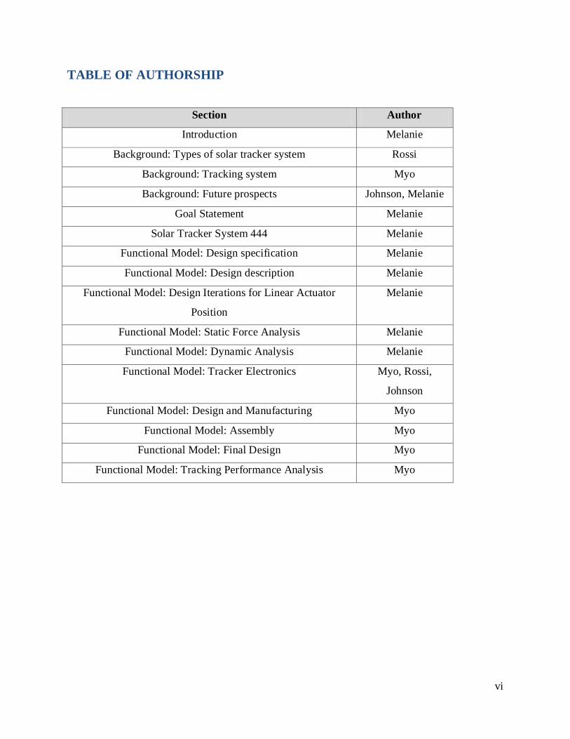
TABLE OF AUTHORSHIP
Section Author
Introduction Melanie
Background: Types of solar tracker system Rossi
Background: Tracking system Myo
Background: Future prospects Johnson, Melanie
Goal Statement Melanie
Solar Tracker System 444 Melanie
Functional Model: Design specification Melanie
Functional Model: Design description Melanie
Functional Model: Design Iterations for Linear Actuator
Position
Melanie
Functional Model: Static Force Analysis Melanie
Functional Model: Dynamic Analysis Melanie
Functional Model: Tracker Electronics Myo, Rossi,
Johnson
Functional Model: Design and Manufacturing Myo
Functional Model: Assembly Myo
Functional Model: Final Design Myo
Functional Model: Tracking Performance Analysis Myo

vii
LIST OF FIGURES
Figure 1: Graph of maximum power output for different kinds of PV trackers 6............................. 2 Figure 2: Graph of measured power output of a panel against angle of incidence .......................... 4 Figure 3: Stationary PV panel orientation 9 ........................................................................................ 4 Figure 4: Earth's axis tilt/orbital path affecting solar angle ............................................................... 5 Figure 5: A horizontal type single-axis tracker................................................................................... 6 Figure 6: A horizontal type single-axis tracker................................................................................... 6 Figure 7: A standard dual-axis tracker ................................................................................................ 7 Figure 8: Flow chart of wind drag analysis comparison between three different methods ........... 12 Figure 9: Forces acting on PV panel at an angle θ where FD and FL are the drag and lift ........... 13 Figure 10: Side view of rapid prototyped reduced scale model at 1:90 scaling ratio .................... 18 Figure 11: Second iteration for the prototype with modification made to the parts ....................... 19 Figure 12: Fixture set-up for the prototype in the wind tunnel to measure drag and lift ............... 20 Figure 13: Force transducer ............................................................................................................... 21 Figure 14: Force probe (left) designed to measure drag moments and lift force. .......................... 21 Figure 15: Schematic section of the prototype in the wind tunnel .................................................. 22 Figure 16: Calibration set-up for the force transducer configuration .............................................. 23 Figure 17: Calibration set-up for the force transducer configuration .............................................. 23 Figure 18: Slot joint to allow for both rotation and translation ....................................................... 24 Figure 19: Streamline representation of the CFD analysis on the symmetry face. ........................ 26 Figure 20: Graph of Drag coefficient against polar angle................................................................ 28 Figure 21: Graph of lift coefficient against polar angle. .................................................................. 29 Figure 22: Graph of corrected drag and lift against polar angle for full scale STS444 ................. 30 Figure 23: Ratio of corrected drag and lift against polar angle ....................................................... 30 Figure 24: Von Mises stress contour graph on the symmetry of the full scale STS444 ................ 32 Figure 25: Safety factor contour graph on the frame part of the full scale STS444....................... 33 Figure 26: Pressure distribution on STS 444 for laminar flow ........................................................ 35 Figure 27: Pressure distribution on STS 444 for turbulent flow...................................................... 35 Figure 28: Schematic of the snow sliding off the rotating panel as a single rigid body ................ 39 Figure 29: Solar tracker assembly showing all parts and constraint type for snow simulation ..... 43 Figure 30: Separation measurement taken between the edge of the snow and panel..................... 44 Figure 31: Separation distance against polar angle ......................................................................... 45 Figure 32: Graph of snow load exerted on panel against polar angle ............................................. 45 Figure 33: Graph of reaction torque at the pin joint O against polar angle. ................................... 46 Figure 34: Graph of torque applied by snow sliding off the panel against polar angle. ................ 47 Figure 35: Graph of resultant torque at pin joint O against polar angle .......................................... 47 Figure 36: Graph of maximum torque against removal time for snow to completely be towed ... 48 Figure 37: Schematic of infinitely long four-bar linkage ................................................................. 52 Figure 38: Side view of iteration 1 with x and y .............................................................................. 54

viii
Figure 39: Graph of y (f(x), g(x)…k(x)) against x distance from center O .................................... 55 Figure 40: Side view of iteration 1 with x and y. ............................................................................. 56 Figure 41: Graph of transmission angle against polar angle. ........................................................... 57 Figure 42: Schematic of the Six-bar mechanism .............................................................................. 58 Figure 43: Lengths of Four-bar “PV_Four-bar” mechanism as calculated in Linkages program. 59 Figure 44: Transmission angle µ2 ...................................................................................................... 59 Figure 45: Model of the six-bar mechanism. .................................................................................... 60 Figure 46: Graph of transmission angle μ1 against polar angle ...................................................... 61 Figure 47: Static reaction forces at connection y .............................................................................. 62 Figure 48: FBD of the four-bar linkage used for the velocity analysis ........................................... 64 Figure 49: Graph of angular velocity ω2 point C against polar angle. ............................................ 65 Figure 50: The functional model modeled in CAD .......................................................................... 66 Figure 51: Graph of polar angle against time ................................................................................... 66 Figure 52: Graph of Angular velocity against polar angle. .............................................................. 67 Figure 53: Graph of Angular acceleration against polar angle ........................................................ 68 Figure 54: Graph of torque (connection between linear actuator and panel) against polar angle . 69 Figure 55: Graph of power required against polar angle ................................................................. 71 Figure 56: Overall tracker electrical system ..................................................................................... 74 Figure 57: SST 175-72M solar panel 22............................................................................................. 75 Figure 58: Experiment setup to compare three types of light sensors ............................................. 76 Figure 59: Voltage divider circuit for the LDRs............................................................................... 76 Figure 60: Voltage output of the PV, LDR and LED with change in degree of light source ........ 77 Figure 61: Using a pair of LDRs as light sensor............................................................................... 77 Figure 62: Error output depending on angle β .................................................................................. 78 Figure 63: Light sensor....................................................................................................................... 79 Figure 64: Operation of the solar sensor ........................................................................................... 80 Figure 65: Piezo vibration sensor ...................................................................................................... 81 Figure 66: Voltage Output vs. Deflection ......................................................................................... 81 Figure 67: ALD110800APCL (ID vs. VDS) .................................................................................... 82 Figure 68: MOSFET Connection for Wind Sensor .......................................................................... 82 Figure 69: Thermal anemometer........................................................................................................ 83 Figure 70: Load sensor ....................................................................................................................... 84 Figure 71: Load sensor output resistance .......................................................................................... 84 Figure 72: Load sensor output voltage .............................................................................................. 85 Figure 73: FSR 406 Force resistive sensor ....................................................................................... 86 Figure 74: ServoCity 6-12V DC 6” stroke linear actuator 20 ........................................................... 86 Figure 75: AM Equipment 214 Series Gearhead Motor 23 .............................................................. 87 Figure 76: Overview design of the functional model ....................................................................... 88 Figure 77: Two vertical cross beams and the center beam connected to the panel ........................ 89 Figure 78: Two tower beams connected to the cross beams ............................................................ 89
ix
Figure 79: Cross section view of the connection .............................................................................. 90 Figure 80: Base legs ........................................................................................................................... 91 Figure 81: Base legs with the turntable attached .............................................................................. 91 Figure 82: Gears assembly inside the base ....................................................................................... 92 Figure 83: Base module assembled ................................................................................................... 92 Figure 84: Attaching the panel and base module.............................................................................. 93 Figure 85: Transportation mode ........................................................................................................ 94 Figure 86: Transporting the tracker ................................................................................................... 94 Figure 89: Assembling the tracker ..................................................................................................... 94 Figure 88: Functional model features ................................................................................................ 95 Figure 89: Functional model at low-drag position ........................................................................... 95 Figure 90: Tracking performance experiment setup......................................................................... 96 Figure 91: Tracking resolution........................................................................................................... 96 Figure 92: Top view of STS444 with dimensions in meters............................................................ 98 Figure 93: Side view of STS444 with dimensions in meters. .......................................................... 98 Figure 94: Front view of STS444 with dimensions in meters. ........................................................ 99 Figure 95: Side View Contour lines of wind velocity coming from inlet. .................................... 100 Figure 96: Project Schematic for the CFD and static structural analysis ...................................... 103 Figure 97: Meshing set-up in ANSYS FLUENT for the fluid box around the STS444. ............. 104 Figure 98: View of the meshing sizing and inflation. .................................................................... 105 Figure 99: Parameters for standard k – ω model in FLUENT set up for CFD analysis. ............. 106 Figure 100: Velocity magnitude, turbulent intensity and turbulent length scale. ......................... 107 Figure 101: The Solution Initialization was computed from the Inlet conditions. ....................... 108 Figure 102: Contour plots representation of the CFD analysis on the symmetry ........................ 108 Figure 103: Meshing sizing and inflation parameters used on the STS444 in Static Structural . 109 Figure 104: View of the 105162 elements on the STS444 symmetry........................................... 109 Figure 105: View of the pressure imported from the CFD analysis onto the STS444................. 110 Figure 106: Resultant reaction force acting on the base of STS444 at wind flow of 89.4 ms-1 . 111 Figure 107: Von Mises stresses on the STS444 ranging from....................................................... 111 Figure 108: Safety factor on the STS444 ranging from 0.284 (red) to 15. ................................... 112 Figure 109: CAD model of the drag and lift fixture used in the wind tunnel testing ................... 115 Figure 110: FBD of the snow sliding along the rotating panel ...................................................... 120 Figure 111: Separation r(θ) against polar angle of the panel ......................................................... 121 Figure 113: Separation distance against time (left) and separation distance against polar angle 124 Figure 114: Schematic of the defined variables of the collector and frame support assembly. .. 129 Figure 115: Calculation sheet and plot of horizontal distance f(x) against x ............................... 130

x
LIST OF TABLES
Table 1: Typical Drag coefficients based on reference area and corresponding drag force .......... 14 Table 2: Corresponding analytical drag and lift coefficients for different polar angle of panel ... 15 Table 3: Parameters and corresponding values for determining Reynolds number ....................... 16 Table 4: Parameters for scaled model ............................................................................................... 18 Table 5: Corresponding experimental drag and lift coefficient for incremental polar angles ....... 24 Table 6: Corresponding simulated drag and lift coefficient for the reduced scale prototype ........ 26 Table 7: Parameters for the reduced prototype and full scale model in the CFD modeling .......... 27 Table 8: Corrected Drag against lift force (ANSYS – real open space one without gap) ............. 27 Table 9: Maximum Von Mises stress based on different polar angles ........................................... 31 Table 10: Terms and definitions of the variables used to derive the differential equation. ........... 40 Table 11: Maximum torque, angle at maximum torque, angle of slip and time ............................. 48 Table 12: Stroke lengths range and product xy for available linear actuator from ServoCity20 .... 54 Table 13: Parameters in the selection of the type of mechanism..................................................... 63 Table 14: Definitions and values for the terms used in deriving the initial linear actuator power 70 Table 15: Definitions and values of the variables used to derive gear power ................................ 72 Table 16: Information about the SST 175-72M panel 22 .................................................................. 75 Table 17: Information about the ServoCity linear actuator ............................................................. 86 Table 18: Information about the AM Equipment 214 Series Gearhead Motor 23 .......................... 87 Table 19: Sum of individual drag owing to the surfaces in direct contact .................................... 102 Table 20: Maximum CL, scaling factor and velocity of wind used for the parameters. ............... 113 Table 21: Typical values obtained during experimental drag with calibration ............................ 117 Table 22: Typical values obtained during experimental lift with calibration ............................... 118 Table 23: List of time for half cycle, total time to slide and corrected time ................................. 123 Table 24: Term and corresponding values used in the determination of magnitude of load ....... 124 Table 25: Terms and definition used to find optimum position of the linear actuator ................. 126 Table 26: Definition of variable terms used to calculate the optimum position ........................... 128 Table 27: List of the different transmission angles for two solutions obtained. ........................... 132 Table 28: Definitions and values for the parameters used in the derivation of reaction forces...137 Table 29: Reaction forces, relation to one another and corresponding mathematical equation.. 138 Table 30: Equation to find mass moment of inertia for individual parts of functional model .... 140 Table 31: Mass moment of Inertia for individual parts in the functional model .......................... 141

xi
TABLE OF CONTENT
EXECUTIVE SUMMARY................................................................................................................ iii ABSTRACT ......................................................................................................................................... iv
ACKNOWLEDGEMENTS ................................................................................................................. v
TABLE OF AUTHORSHIP ............................................................................................................... vi LIST OF FIGURES ............................................................................................................................vii
LIST OF TABLES................................................................................................................................ x
TABLE OF CONTENT ...................................................................................................................... xi 1. INTRODUCTION.................................................................................................................... 1
2. BACKGROUND ...................................................................................................................... 3
2.1. Types of solar tracker systems .......................................................................................... 5
2.1.1. Single-axis Tracker .................................................................................................... 5
2.1.2. Dual-axis Tracker ....................................................................................................... 6
2.2. Tracking system ................................................................................................................. 7
2.2.1. Passive Tracking ........................................................................................................ 7
2.2.2. Active Tracking .......................................................................................................... 7
2.3. Future prospects ................................................................................................................. 8
2.3.1. Efficiency ................................................................................................................... 8
2.3.2. Reliability ................................................................................................................... 8
2.3.3. Investment Capital and Pay Back ............................................................................. 9
2.3.4. Feasibility ................................................................................................................... 9
3. GOAL STATEMENT ............................................................................................................ 10
4. SOLAR TRACKER SYSTEM 444 ...................................................................................... 11
4.1. Wind load analysis........................................................................................................... 11
4.1.1. Analytical Approach ................................................................................................ 13
4.1.2. Wind Tunnel Testing ............................................................................................... 15
4.1.3. Simulated Approach ................................................................................................ 25
4.1.4. Results....................................................................................................................... 27
4.1.5. Discussion................................................................................................................. 34
4.1.6. Summary................................................................................................................... 37
4.2. Snow Load Analysis ........................................................................................................ 38

xii
4.2.1. Background .............................................................................................................. 38
4.2.2. Snow Torque Profile ................................................................................................ 39
4.2.3. Mechanism Analysis ................................................................................................ 43
4.2.4. Results and Discussion ............................................................................................ 44
4.2.5. Summary................................................................................................................... 49
4.3. Conclusions and Recommendations ............................................................................... 49
5. FUNCTIONAL MODEL....................................................................................................... 51
5.1. Design Specifications ...................................................................................................... 51
5.2. Design Description .......................................................................................................... 52
5.2.1. System Kinematics................................................................................................... 52
5.2.2. Linear actuator positioning ...................................................................................... 52
5.3. Design Iterations for Linear Actuator Positioning ........................................................ 54
5.3.1. Design Iteration 1 ..................................................................................................... 54
5.3.2. Design Iteration 2 ..................................................................................................... 56
5.3.3. Design Iteration 3 ..................................................................................................... 58
5.4. Static Force Analysis ....................................................................................................... 61
5.4.1. Design Iteration 1 ..................................................................................................... 61
5.4.2. Design iteration 2 ..................................................................................................... 62
5.4.3. Design Iteration 3 ..................................................................................................... 62
5.4.4. Selection of linear actuator mechanism .................................................................. 62
5.5. Dynamic Analysis............................................................................................................ 63
5.5.1. Velocity Analysis of the four-bar linkage .............................................................. 63
5.5.2. Power Analysis......................................................................................................... 70
5.5.3. State equation for the system motion...................................................................... 72
5.6. Tracker Electronics .......................................................................................................... 73
5.6.1. Panel.......................................................................................................................... 74
5.6.2. Light sensor .............................................................................................................. 76
5.6.3. Wind sensor .............................................................................................................. 80
5.6.4. Load sensor............................................................................................................... 83
5.6.5. Linear Actuator ........................................................................................................ 86
5.6.6. DC Motor.................................................................................................................. 87

xiii
5.7. Design and Manufacturing .............................................................................................. 88
5.7.1. Panel Assembly ........................................................................................................ 88
5.7.2. Base Assembly ......................................................................................................... 90
5.8. Assembly .......................................................................................................................... 92
5.9. Final design ...................................................................................................................... 95
5.10. Tracking Performance Analysis .................................................................................. 96
5.11. Conclusion .................................................................................................................... 97
APPENDIX A ..................................................................................................................................... 98
APPENDIX B ................................................................................................................................... 100
APPENDIX C ................................................................................................................................... 103
APPENDIX D ................................................................................................................................... 113
APPENDIX E ................................................................................................................................... 115
APPENDIX F.................................................................................................................................... 116
APPENDIX G ................................................................................................................................... 119
APPENDIX H ................................................................................................................................... 126
APPENDIX I..................................................................................................................................... 128
APPENDIX J .................................................................................................................................... 133
APPENDIX K ................................................................................................................................... 140
APPENDIX L ................................................................................................................................... 142
APPENDIX M .................................................................................................................................. 146
APPENDIX N ................................................................................................................................... 148
REFERENCES ................................................................................................................................. 155

1
1. INTRODUCTION
Solar power is the fastest growing means of renewable energy production. Globally, the grid-
connected solar capacity increased on average by 60% annually from 2004 to 2009 according to
the National Center for Policy Analysis 1. Yet solar energy only contributed 0.18% 2 of the total
energy produced in the United States in 2011. Of many types of solar energy, the photovoltaic
(PV) solar cell technology, has only improved by 0.10% of its total US energy contribution from
2010 to 2011 3. However, future of PV solar technologies is promising considering favorable
location and continued federal tax subsidies 1 as well as state renewable standard protocol 4. With
the continued trend in decreasing cost of PV panels and government subsidies, PV solar energy
might become cost competitive in the next 10 years (subsidy-free), for commercial installations
while utility-scale installations might take longer 1. The August 2010 White House report, on the
other hand, predicted that PV solar power will reach grid parity by 2015.
One way to increase the energy collected from the PV panels is by tracking the sun. Novel Dual-
Axis solar trackers allow precise control of the polar and azimuth angle of the panel, allowing
the panel to always be perpendicular to the sunlight. Tracking the sun can potentially double the
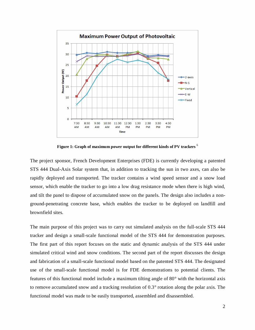
energy output of a fixed PV solar system 5. Figure 1 compared the power output of four different
kinds of tracker (dual-axis, North-South, vertical, East-West) to the power output of a fixed
panel 6. Figure 1 indicates an increase of output power gain up to 43.87%, 37.53%, 34.43% and
15.69% for the dual-axes, east–west, vertical and north–south trackers, respectively, as compared
with the fixed mounted panel. The dual-axis trackers produce the maximum power compare to
other types of trackers.
2
Figure 1: Graph of maximum power output for different kinds of PV trackers 6
The project sponsor, French Development Enterprises (FDE) is currently developing a patented
STS 444 Dual-Axis Solar system that, in addition to tracking the sun in two axes, can also be
rapidly deployed and transported. The tracker contains a wind speed sensor and a snow load
sensor, which enable the tracker to go into a low drag resistance mode when there is high wind,
and tilt the panel to dispose of accumulated snow on the panels. The design also includes a non-
ground-penetrating concrete base, which enables the tracker to be deployed on landfill and
brownfield sites.
The main purpose of this project was to carry out simulated analysis on the full-scale STS 444
tracker and design a small-scale functional model of the STS 444 for demonstration purposes.
The first part of this report focuses on the static and dynamic analysis of the STS 444 under
simulated critical wind and snow conditions. The second part of the report discusses the design
and fabrication of a small-scale functional model based on the patented STS 444. The designated
use of the small-scale functional model is for FDE demonstrations to potential clients. The
features of this functional model include a maximum tilting angle of 80° with the horizontal axis
to remove accumulated snow and a tracking resolution of 0.3° rotation along the polar axis. The
functional model was made to be easily transported, assembled and disassembled.
3
2. BACKGROUND
The power output of a solar panel depends on the efficiency of the solar cell and the intensity of
light falling on the cell. The efficiency depends on cell technology, which determines the price
of the solar panel and the power output per square area.
The type of cell commercially in use today is the crystalline silicon cell, which is around
13%~20% efficient. Standard Test Conditions (STC) of 1,000 W/m2 solar irradiance and 25°C
PV module temperature are used for testing PV cells. So for a cell that is 20% efficient, it
produces 200 W of usable power per meter square.
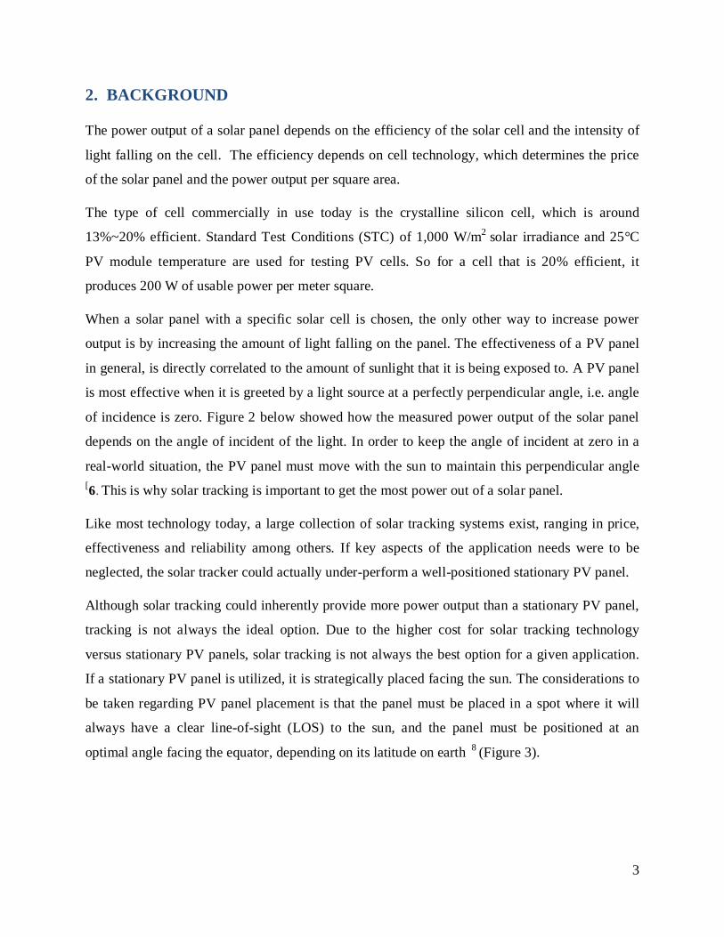
When a solar panel with a specific solar cell is chosen, the only other way to increase power
output is by increasing the amount of light falling on the panel. The effectiveness of a PV panel
in general, is directly correlated to the amount of sunlight that it is being exposed to. A PV panel
is most effective when it is greeted by a light source at a perfectly perpendicular angle, i.e. angle
of incidence is zero. Figure 2 below showed how the measured power output of the solar panel
depends on the angle of incident of the light. In order to keep the angle of incident at zero in a
real-world situation, the PV panel must move with the sun to maintain this perpendicular angle [6. This is why solar tracking is important to get the most power out of a solar panel.
Like most technology today, a large collection of solar tracking systems exist, ranging in price,
effectiveness and reliability among others. If key aspects of the application needs were to be
neglected, the solar tracker could actually under-perform a well-positioned stationary PV panel.
Although solar tracking could inherently provide more power output than a stationary PV panel,
tracking is not always the ideal option. Due to the higher cost for solar tracking technology
versus stationary PV panels, solar tracking is not always the best option for a given application.
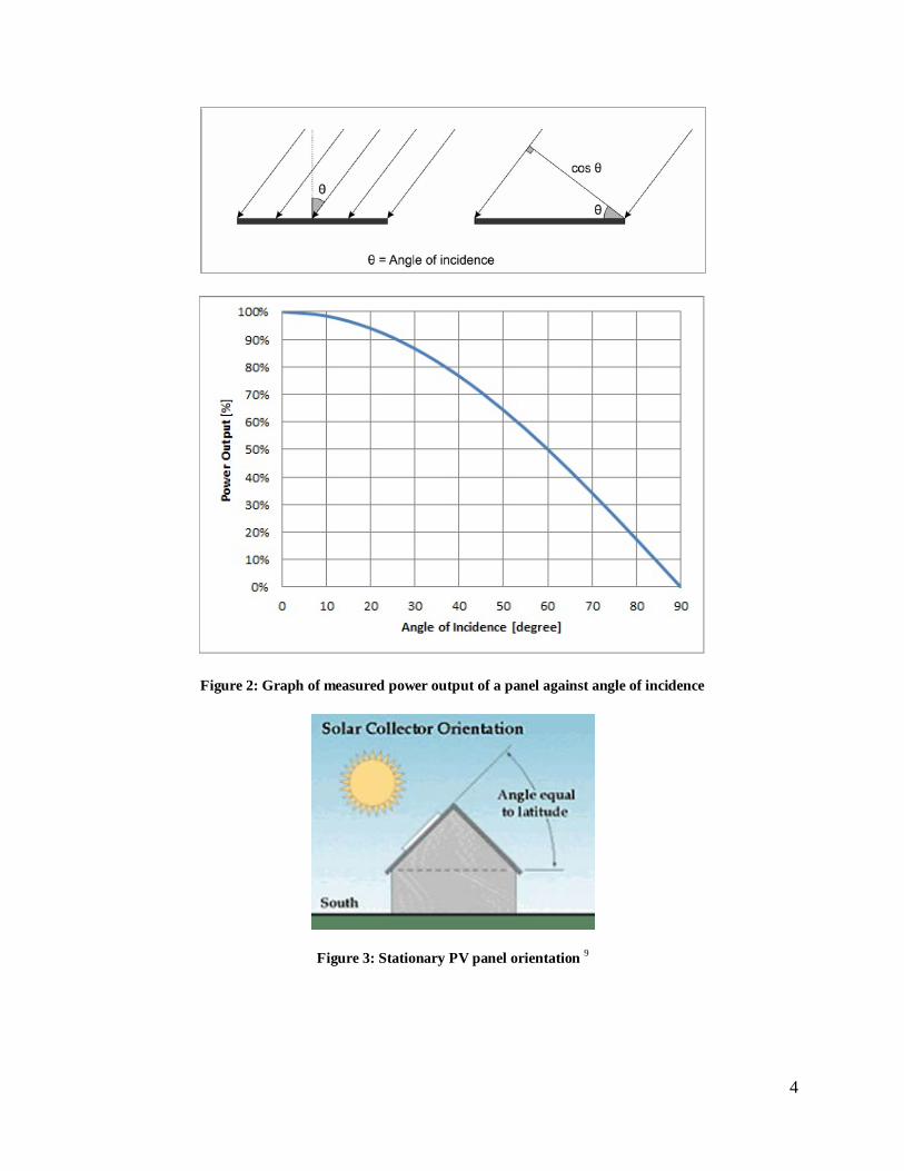
If a stationary PV panel is utilized, it is strategically placed facing the sun. The considerations to
be taken regarding PV panel placement is that the panel must be placed in a spot where it will
always have a clear line-of-sight (LOS) to the sun, and the panel must be positioned at an
optimal angle facing the equator, depending on its latitude on earth 8 (Figure 3).
4
Figure 2: Graph of measured power output of a panel against angle of incidence
Figure 3: Stationary PV panel orientation 9
5
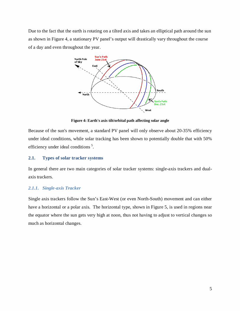
Due to the fact that the earth is rotating on a tilted axis and takes an elliptical path around the sun
as shown in Figure 4, a stationary PV panel’s output will drastically vary throughout the course
of a day and even throughout the year.
Figure 4: Earth's axis tilt/orbital path affecting solar angle
Because of the sun's movement, a standard PV panel will only observe about 20-35% efficiency
under ideal conditions, while solar tracking has been shown to potentially double that with 50%
efficiency under ideal conditions 5.
2.1. Types of solar tracker systems
In general there are two main categories of solar tracker systems: single-axis trackers and dual-
axis trackers.
2.1.1. Single-axis Tracker
Single axis trackers follow the Sun’s East-West (or even North-South) movement and can either
have a horizontal or a polar axis. The horizontal type, shown in Figure 5, is used in regions near
the equator where the sun gets very high at noon, thus not having to adjust to vertical changes so
much as horizontal changes.

6
Figure 5: A horizontal type single-axis tracker
The polar type single-axis trackers, shown in Figure 6, is used in high latitudes where the sun
does not get very high, but where summer days can be longer, thus using the fact that vertical
movement does not have to be compensated for as much as horizontal movement. Polar type
single-axis trackers are good for regions near the north or south poles 10.
Figure 6: A horizontal type single-axis tracker
2.1.2. Dual-axis Tracker
Two-axis or dual-axis trackers, shown in Figure 7, follow the sun’s movement irrespective of the
axis of rotation. Dual-axis solar trackers have both a horizontal and a vertical axis and thus they
can track the sun's apparent motion in the sky, no matter where it is positioned on earth. Having
dual-axis motion maximizes the total power output by keeping the panels in direct sunlight
longer than single-axis trackers or stationary panels 9,10.

7
Figure 7: A standard dual-axis tracker
2.2. Tracking system
Solar tracking system can be classified into two main types: passive tracking and active tracking.
2.2.1. Passive Tracking
Passive trackers use compressed gas to move the tracker. Depending on the angle of sunlight
with the gas containers, a difference in gas pressure is created. This moves the tracker until it
gets to an equilibrium position. The advantage of passive tracker is that the tracking system does
not require a controller. But passive trackers are slow in response and are vulnerable to wind
gusts.
2.2.2. Active Tracking
Active tracking uses an electromechanical system to position the solar tracker to keep the panel
perpendicular to the sun. Trackers that use sensors to track the sun’s position input data into the
controller unit, which drives the motors and actuators to position the tracker. There are trackers
that use a solar map. Depending on the location, a solar map gives information on where the sun
is at different times of day throughout the year. Trackers that use a solar map do not need sensors
to track the sun. Some trackers use both sensors and a solar map. During sunny weather, the
sensors would be used to track the sun. During cloudy conditions, the information from the solar
map would be used. It is important to track the sun even in cloudy conditions since solar panels
can still produce produces energy under those conditions.

8
2.3. Future prospects
The debate on solar energy production is a controversial one with concern about the efficiency,
reliability and, above all, the commercial feasibility pertaining to the investment cost and grid
parity of the system. Government subsidies have encouraged research and development of PV
solar system as the alternative to natural gas which is the biggest competitor in the production of
electricity. However, skeptics are still dubious about solar power potential. In the limit that solar
power may take another century to be the sole provider of electricity for the whole world, there
are great expectations that it will be able to provide for more than the 0.2% energy contribution 2.
2.3.1. Efficiency
The efficiency of a dual-axis PV solar system, under ideal conditions, is 20-35% higher than
fixed PV solar systems. However, Mousazadeh et al. found that solar tracking could potentially
double the efficiency under ideal conditions 5. With sunlight variations due to the earth rotation
and cloud cover, the average electrical power obtainable over a year would be about 20% of its
peak wattage 5. Another published article conducted in Jordan have reported increases in power
gain of up to 43.87% in dual-axis tracking as compared to 15.69% for North-South tracking 6.
Despite the fact that solar cells can last 20 to 25 years, output power is reported to decline by
approximately 0.5% per year, even with periodic maintenance. This implies that by the end of 20
years they will only produce, at max, 80% of their rated capacity which will amount to only 16%
of their peak wattage under ideal conditions 1.
2.3.2. Reliability
One of the biggest advantages of the conversion of solar energy to electricity via photovoltaic
means is the autonomy of each solar panel collector 11. Most solar panels are connected in
parallel so that in the event of a defective panel, it will not affect the other panels and can be
easily replaced without affecting the whole connected system.
Despite the long-term benefits of solar energy, the biggest problems remain the low energy
generation and the energy storage ability.

9
2.3.3. Investment Capital and Pay Back
Currently, subsidized solar energy costs between $0.22 per kilowatt-hour and $0.30 per kilowatt-
hour, according to independent analyses. By contrast, the average cost of electricity nationwide
is expected to remain roughly $0.11 per kilowatt-hour through 2015 1. The cost for at home
installation is estimated at around $5,000 11 and it is difficult to determine the exact time for pay
back considering the declining performance of the PV cells and other factors such as economic
inflation.
2.3.4. Feasibility
The most important concern for investing in solar energy production is the time required for the
subsidies to remain in place for these systems to be autonomously profitable and feasible. The
fact that the price point of grid parity depends on a number of variables such as the amount of
sunlight an area receives, the orientation of the solar array, whether the solar arrays are fixed or
track the sun, construction costs and financing options, resulted in significance difference in
breakeven costs by more than a factor of 10 1. Nevertheless, grid disparity was reached in Hawaii
where the average price for electricity was $0.41 1, 12. Arizona is another location which receives
abundant sunlight and where grid parity would have been reached if not for its limited
transmission access and low electricity prices 1.
Despite these economic factors as well as practical concerns, solar power could become the most
important power source if the technology catches up to increase the efficiency of the
photovoltaic collection and the means by which the energy is collected.

10
3. GOAL STATEMENT
This project had two main goals as specified by the sponsor:
(i) To conduct wind and snow load analyses on the STS 444 to determine the maximum
force and stress acting on the system at different panel polar angles.
(ii) To design and build a small-scale functional prototype to demonstrate tracking abilities of
the STS 444. The sponsor would be using this model to showcase to its future customers.
11
4. SOLAR TRACKER SYSTEM 444
The STS 444 is a second generation dual-axis solar tracker under development by FDE. The
analyses completed in this report were accomplished using a model based on preliminary
blueprints of the STS 444 provided by FDE with rough dimension estimates.
The following sections provide detailed discussion on the wind and snow load analyses using the
full-scale STS 444 model. Data were compared via non-dimensional values for ease of
application to similar systems.
4.1. Wind load analysis
Of all the loads that solar tracker systems are subjected to, wind load is the most important as it
is responsible for the largest loading forces that vary in all direction and can cause mechanical
damage due to resonance. In this report, only the most critical configurations of the STS 444 will
be analyzed against a specified one-directional wind velocity of 89.4 ms-1 (200mph).
The forces acting on the STS 444 were calculated using three approaches: analytical, simulated
and experimental methods (Figure 8). Estimate of forces were obtained from the full scale STS
444 and used to find the scaling factor for the experimental wind tunnel testing. The same
conditions used in the wind tunnel were simulated to compare with the experimental data. Once
validated, correction was made on the simulation for the full scale STS 444. Force data were
collected at different tilt angle θ as shown in Figure 9 of the PV collector and compared for the
three different approaches.. A good analysis is one in which the three approaches – analytical,
simulated and experimental - yield relatively close values.
12
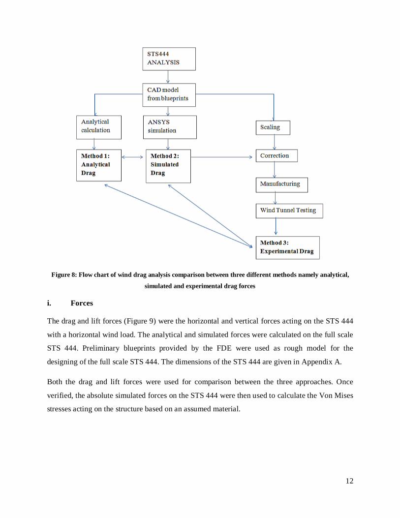
Figure 8: Flow chart of wind drag analysis comparison between three different methods namely analytical,
simulated and experimental drag forces
i. Forces
The drag and lift forces (Figure 9) were the horizontal and vertical forces acting on the STS 444
with a horizontal wind load. The analytical and simulated forces were calculated on the full scale
STS 444. Preliminary blueprints provided by the FDE were used as rough model for the
designing of the full scale STS 444. The dimensions of the STS 444 are given in Appendix A.
Both the drag and lift forces were used for comparison between the three approaches. Once
verified, the absolute simulated forces on the STS 444 were then used to calculate the Von Mises
stresses acting on the structure based on an assumed material.
13
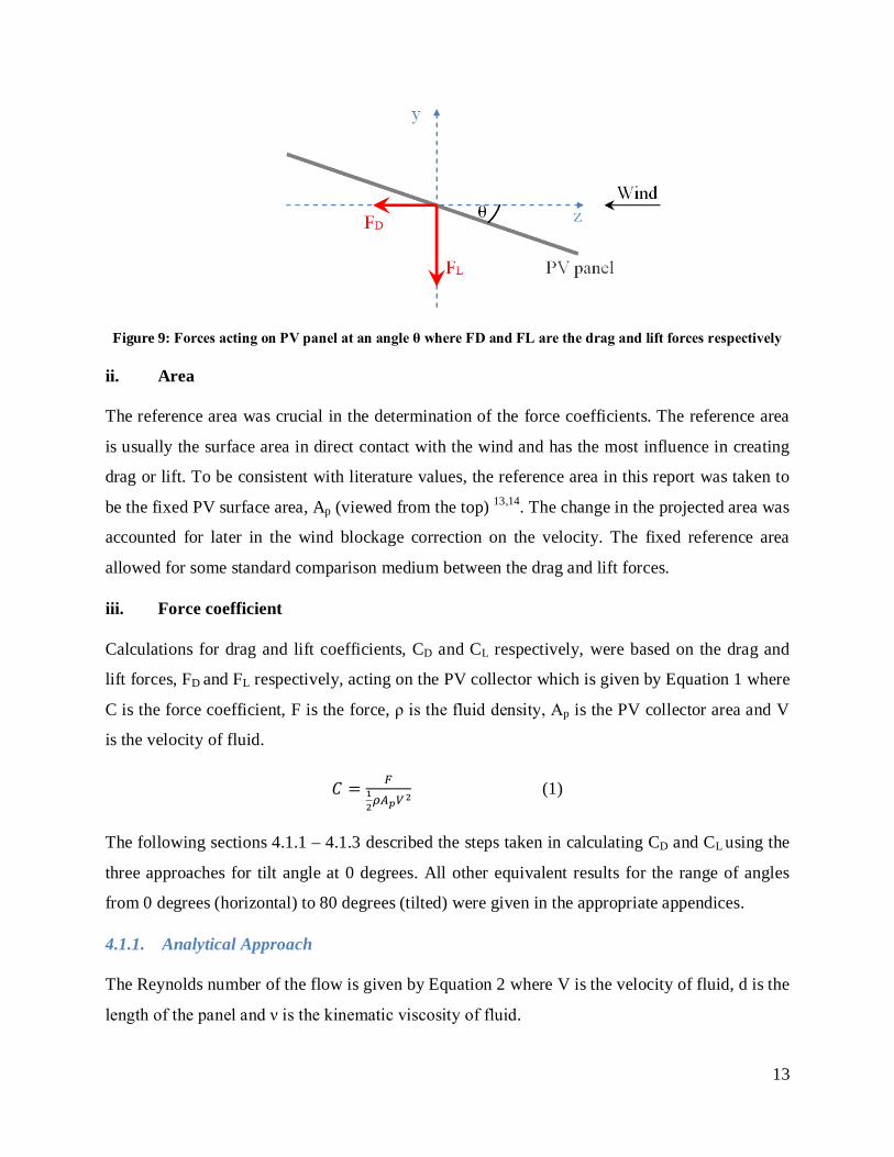
Figure 9: Forces acting on PV panel at an angle θ where FD and FL are the drag and lift forces respectively
ii. Area
The reference area was crucial in the determination of the force coefficients. The reference area
is usually the surface area in direct contact with the wind and has the most influence in creating
drag or lift. To be consistent with literature values, the reference area in this report was taken to
be the fixed PV surface area, Ap (viewed from the top) 13,14. The change in the projected area was
accounted for later in the wind blockage correction on the velocity. The fixed reference area
allowed for some standard comparison medium between the drag and lift forces.
iii. Force coefficient
Calculations for drag and lift coefficients, CD and CL respectively, were based on the drag and
lift forces, FD and FL respectively, acting on the PV collector which is given by Equation 1 where
C is the force coefficient, F is the force, ρ is the fluid density, Ap is the PV collector area and V
is the velocity of fluid.
𝐶 = 𝐹12𝜌𝐴𝑝𝑉
2 (1)
The following sections 4.1.1 – 4.1.3 described the steps taken in calculating CD and CL using the
three approaches for tilt angle at 0 degrees. All other equivalent results for the range of angles
from 0 degrees (horizontal) to 80 degrees (tilted) were given in the appropriate appendices.
4.1.1. Analytical Approach
The Reynolds number of the flow is given by Equation 2 where V is the velocity of fluid, d is the
length of the panel and ν is the kinematic viscosity of fluid.

14
𝑅𝑒 = 𝑉𝑑𝜈
(2)
The Reynolds number given V = 89.4 ms-1, d = 22.86 m and ν = 1.57 x 10⁻⁵ Pa.s along the length
of the PV collector was calculated to be 1.3 × 10⁸. This indicated that the general flow was fully
turbulent.
Table 1 shows the drag forces broken down by parts considered to contribute to total drag forces as calculated in Appendix B.
Table 1: Typical Drag coefficients based on reference area and corresponding drag force for each part in the
STS444 for angle at 0 degree
Part CD based on CD FD (105 N)
PV collector Platform area 0.00215 0.0383
Horizontal beams x2 Frontal area 2.1 0.0066
Frame support x2 Frontal area ~ 1.8 0.1320
Rectangular turntable Platform area 0.00744 0.0050
Gear Circular cylinder ~ 2.2 0.1512
Base Frontal area ~ 1.2 0.7707
Total Analytical Force 1.104
For air density ρ, PV collector area Ap and velocity V of air at 1.184 kg.m-3, 188.1 m2 and 89.4
ms-1 respectively, analytical CD were determined to be 0.124 at polar angle θ of 0 degree.
Calculated analytical drag could vary as much as + 10000N from estimation of individual CD, so
that final CD for the STS 444 could vary by + 0.01.
Lift forces, FL, are more complicated to calculate and require solving the boundary layer
differential equation. A simplified estimate of the lift was obtained using Equation 3 which is the
vertical component of the drag.
𝐹𝐿 = 𝐹𝐷𝑡𝑎𝑛𝜃
(3)
CD and CL were calculated for each increment polar angle θ of 10 degrees from 0 – 80 degrees
tilt angle and listed in are listed in Table 2.
15
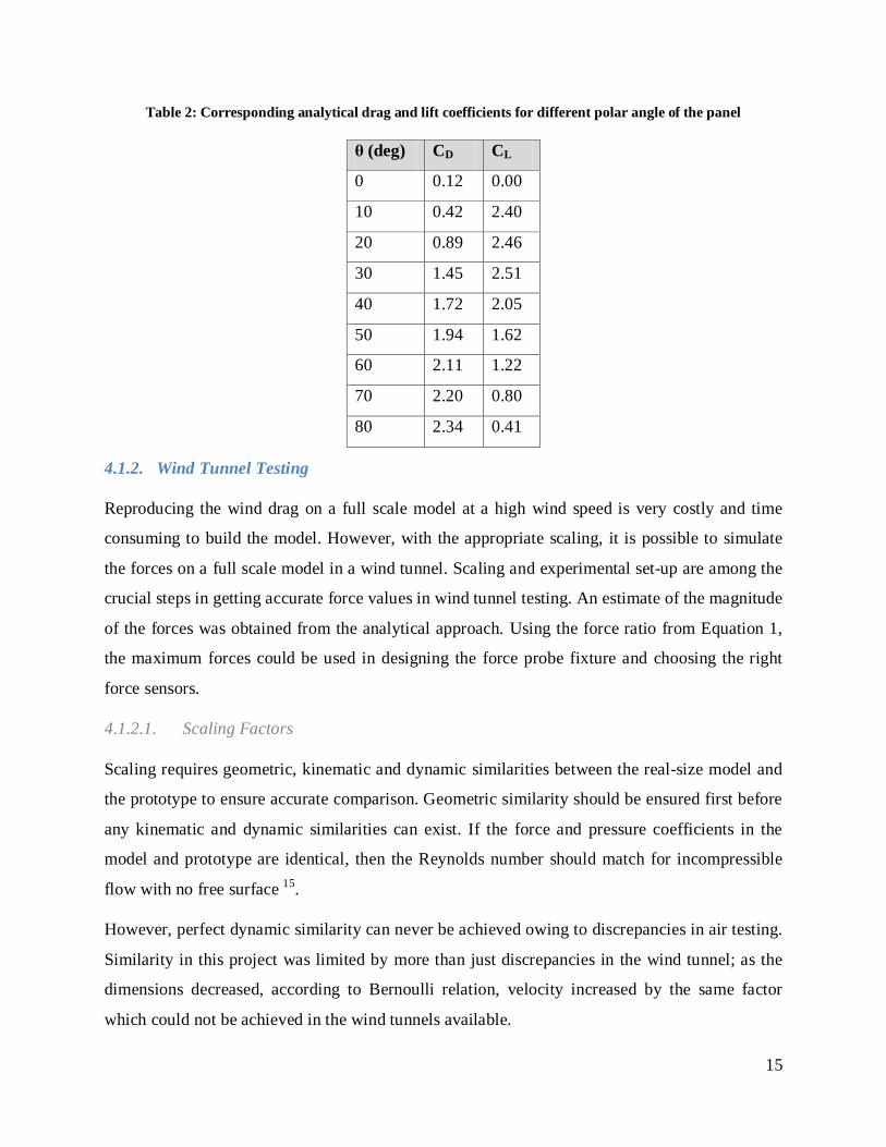
Table 2: Corresponding analytical drag and lift coefficients for different polar angle of the panel
θ (deg) CD CL
0 0.12 0.00
10 0.42 2.40
20 0.89 2.46
30 1.45 2.51
40 1.72 2.05
50 1.94 1.62
60 2.11 1.22
70 2.20 0.80
80 2.34 0.41
4.1.2. Wind Tunnel Testing
Reproducing the wind drag on a full scale model at a high wind speed is very costly and time
consuming to build the model. However, with the appropriate scaling, it is possible to simulate
the forces on a full scale model in a wind tunnel. Scaling and experimental set-up are among the
crucial steps in getting accurate force values in wind tunnel testing. An estimate of the magnitude
of the forces was obtained from the analytical approach. Using the force ratio from Equation 1,
the maximum forces could be used in designing the force probe fixture and choosing the right
force sensors.
4.1.2.1. Scaling Factors
Scaling requires geometric, kinematic and dynamic similarities between the real-size model and
the prototype to ensure accurate comparison. Geometric similarity should be ensured first before
any kinematic and dynamic similarities can exist. If the force and pressure coefficients in the
model and prototype are identical, then the Reynolds number should match for incompressible
flow with no free surface 15.
However, perfect dynamic similarity can never be achieved owing to discrepancies in air testing.
Similarity in this project was limited by more than just discrepancies in the wind tunnel; as the
dimensions decreased, according to Bernoulli relation, velocity increased by the same factor
which could not be achieved in the wind tunnels available.

16
The Reynolds number along both the width and length of the PV collector was calculated to be
completely turbulent as listed in Table 3.
Table 3: Parameters and corresponding values for determining Reynolds number on the panel of the full
scale STS 444
Parameters Definition Value
dL (length) (m) Length of PV collector 22.86
dW (width) (m) Width of the PV collector 8.230
V* (ms-1) Maximum wind velocity 89.4
𝜈 (m2s-1) (25 C) Kinematic viscosity (x 10-5) 1.57
ReL Reynolds number (along length) (x108) 1.30
ReW Reynolds number (along width) (x107) 4.70
*1 mph = 0.447 m/s
4.1.2.2. Scaling Methods
There are three methods to determine the scaling factor of a model in wind tunnel testing: Reynolds number, force ratio and blockage factor.
i. Reynolds number:
For low wind velocity (< 200mph), compressibility effects are negligible. This means that
viscosity effects which are equivalent to the Reynolds number become more relevant than the
Mach number.
Since Reynolds number along both length and width are fully turbulent, trying to keep the
Reynolds number for the scaled model consistent with the Reynolds number for the full scale
model is very difficult at such high value. The resulting velocity for the reduced scale model
would be too high to reproduce. It could only be ensured that the final flow for the reduced
prototype is turbulent.
ii. Force ratio:
By using analytical and simulated analysis to get an estimate of the resulting drag and moment at
the base of the model, CD and CL can be calculated using Equation 2.
17
The panel area Ap is consistently used in all the calculations and the corresponding scaling factor is determined.
iii. Blockage factor:
By using analytical and simulated analysis, an estimate of the resulting drag and moment at the
base of the model was found. The aspect ratio of the model surface area perpendicular to the
wind flow and the cross-sectional area of the wind tunnel was calculated. Based on blockage
correction a scaling factor was determined.
Among the many blockage correction methodologies available are those of Glauert, Maskell,
Ashill & Keating, Hensel, Hackett-Wilsden and Sorensen & Mikkelsen.
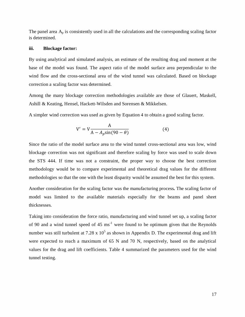
A simpler wind correction was used as given by Equation 4 to obtain a good scaling factor.
V′ = VA
A − 𝐴𝑝sin (90 − 𝜃) (4)
Since the ratio of the model surface area to the wind tunnel cross-sectional area was low, wind
blockage correction was not significant and therefore scaling by force was used to scale down
the STS 444. If time was not a constraint, the proper way to choose the best correction
methodology would be to compare experimental and theoretical drag values for the different
methodologies so that the one with the least disparity would be assumed the best for this system.
Another consideration for the scaling factor was the manufacturing process. The scaling factor of
model was limited to the available materials especially for the beams and panel sheet
thicknesses.
Taking into consideration the force ratio, manufacturing and wind tunnel set up, a scaling factor
of 90 and a wind tunnel speed of 45 ms-1 were found to be optimum given that the Reynolds
number was still turbulent at 7.28 x 10⁵ as shown in Appendix D. The experimental drag and lift
were expected to reach a maximum of 65 N and 70 N, respectively, based on the analytical
values for the drag and lift coefficients. Table 4 summarized the parameters used for the wind
tunnel testing.

18
Table 4: Parameters for scaled model
Parameters Value
Scaling factor 90
Wind tunnel datum Velocity (ms-1) 45
Reynolds number (PV collector) (x 105) 7.28
Estimated max Drag at the base (N) 65
Estimated max Lift at the base (N) 70
4.1.2.3. Scale Model Design and Fabrication
i. Reduced scale model
The reduced scale prototype was based mostly on the design model used for the analytical
analysis given in Appendix A.
The first iteration was that of a rigid rapid prototyped body (Figure 10) which had no degrees of
freedom and with the panel at the default horizontal position. The support beams were removed
and replaced by a flat sheet through which the panel could be screwed in while keeping the
surface area hit by the wind consistent with the real scale model. A support was added at the
bottom of the base through which the force probe would be secured (Figure 10).
Figure 10: Side view of rapid prototyped reduced scale model at 1:90 scaling ratio
The next iteration was fabricated completely out of a combination of Aluminum sheet for the
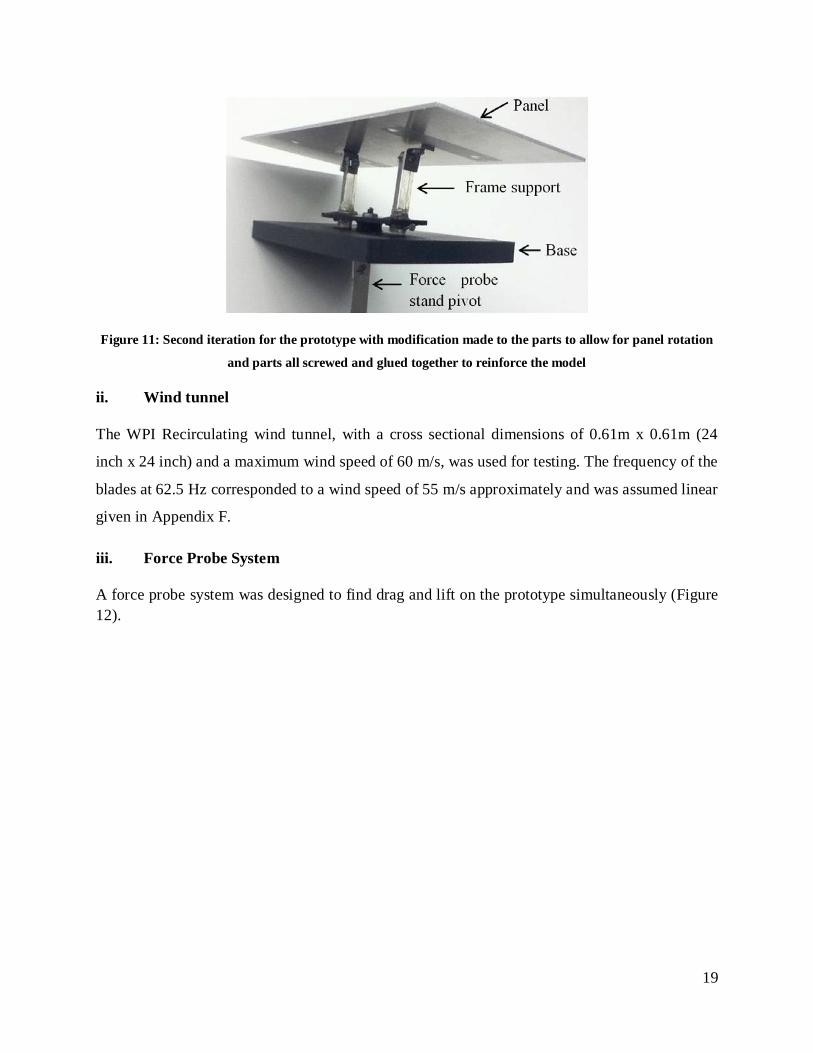
panel, acrylic for frame support and rapid prototyping for more complex parts (Figure 11). This
second prototype was made to be able to vary the polar angle of the panel and find the
corresponding drag and lift exerted at the base. The prototype was assembled with screws and
glue at appropriate places.
19
Figure 11: Second iteration for the prototype with modification made to the parts to allow for panel rotation
and parts all screwed and glued together to reinforce the model
ii. Wind tunnel
The WPI Recirculating wind tunnel, with a cross sectional dimensions of 0.61m x 0.61m (24
inch x 24 inch) and a maximum wind speed of 60 m/s, was used for testing. The frequency of the
blades at 62.5 Hz corresponded to a wind speed of 55 m/s approximately and was assumed linear
given in Appendix F.
iii. Force Probe System
A force probe system was designed to find drag and lift on the prototype simultaneously (Figure 12).
20
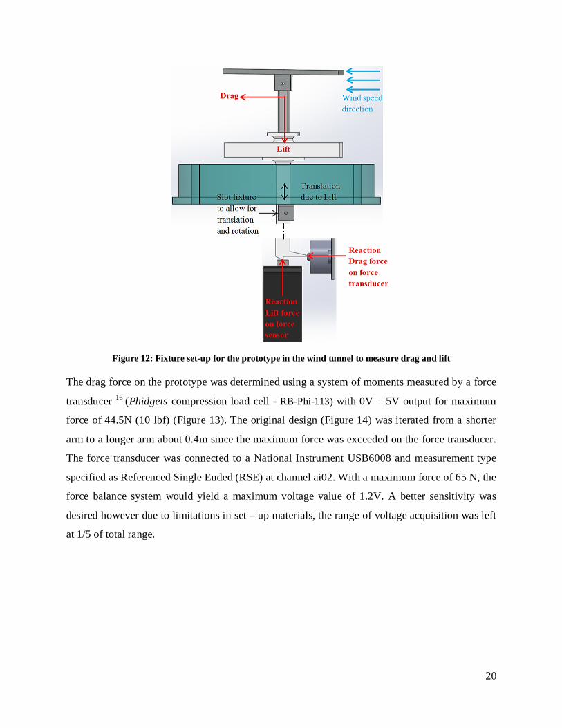
Figure 12: Fixture set-up for the prototype in the wind tunnel to measure drag and lift
The drag force on the prototype was determined using a system of moments measured by a force
transducer 16 (Phidgets compression load cell - RB-Phi-113) with 0V – 5V output for maximum
force of 44.5N (10 lbf) (Figure 13). The original design (Figure 14) was iterated from a shorter
arm to a longer arm about 0.4m since the maximum force was exceeded on the force transducer.
The force transducer was connected to a National Instrument USB6008 and measurement type
specified as Referenced Single Ended (RSE) at channel ai02. With a maximum force of 65 N, the
force balance system would yield a maximum voltage value of 1.2V. A better sensitivity was
desired however due to limitations in set – up materials, the range of voltage acquisition was left
at 1/5 of total range.
21
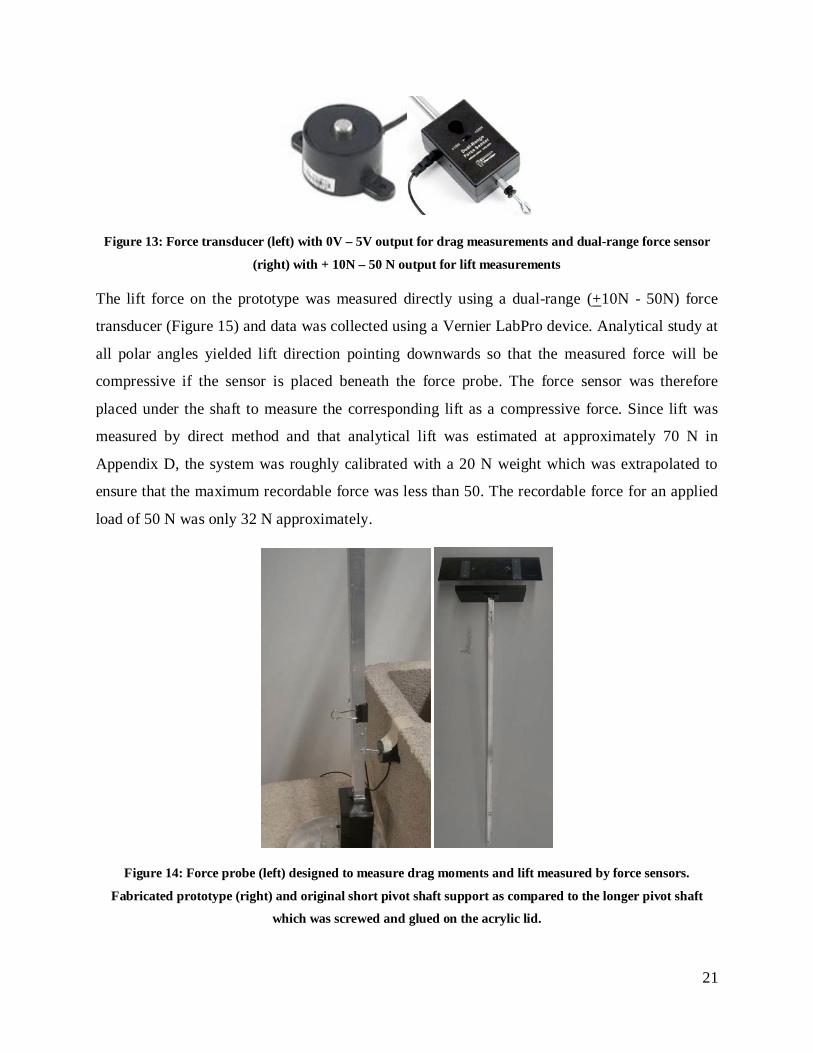
Figure 13: Force transducer (left) with 0V – 5V output for drag measurements and dual-range force sensor
(right) with + 10N – 50 N output for lift measurements
The lift force on the prototype was measured directly using a dual-range (+10N - 50N) force
transducer (Figure 15) and data was collected using a Vernier LabPro device. Analytical study at
all polar angles yielded lift direction pointing downwards so that the measured force will be
compressive if the sensor is placed beneath the force probe. The force sensor was therefore
placed under the shaft to measure the corresponding lift as a compressive force. Since lift was
measured by direct method and that analytical lift was estimated at approximately 70 N in
Appendix D, the system was roughly calibrated with a 20 N weight which was extrapolated to
ensure that the maximum recordable force was less than 50. The recordable force for an applied
load of 50 N was only 32 N approximately.
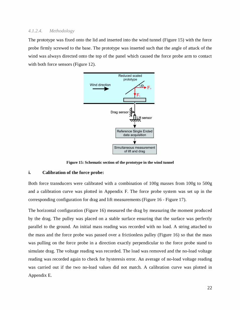
Figure 14: Force probe (left) designed to measure drag moments and lift measured by force sensors.
Fabricated prototype (right) and original short pivot shaft support as compared to the longer pivot shaft
which was screwed and glued on the acrylic lid.
22
4.1.2.4. Methodology
The prototype was fixed onto the lid and inserted into the wind tunnel (Figure 15) with the force
probe firmly screwed to the base. The prototype was inserted such that the angle of attack of the
wind was always directed onto the top of the panel which caused the force probe arm to contact
with both force sensors (Figure 12).
Figure 15: Schematic section of the prototype in the wind tunnel
i. Calibration of the force probe:
Both force transducers were calibrated with a combination of 100g masses from 100g to 500g
and a calibration curve was plotted in Appendix F. The force probe system was set up in the
corresponding configuration for drag and lift measurements (Figure 16 - Figure 17).
The horizontal configuration (Figure 16) measured the drag by measuring the moment produced
by the drag. The pulley was placed on a stable surface ensuring that the surface was perfectly
parallel to the ground. An initial mass reading was recorded with no load. A string attached to
the mass and the force probe was passed over a frictionless pulley (Figure 16) so that the mass
was pulling on the force probe in a direction exactly perpendicular to the force probe stand to
simulate drag. The voltage reading was recorded. The load was removed and the no-load voltage
reading was recorded again to check for hysteresis error. An average of no-load voltage reading
was carried out if the two no-load values did not match. A calibration curve was plotted in
Appendix E.

23
Figure 16: Calibration set-up for the force transducer configuration with mass pulling perpendicularly to the
pivot stand to simulate drag
The vertical configuration (Figure 17) allowed for lift measurement alone since drag produced a
moment and lift produced a translational displacement assumed to pass directly through the
pivot. Therefore by restricting the rotation of the arm and allowing only for translation, the lift
component can be measured (in this case the rotation restriction was provided by the force
transducer measuring drag simultaneously). Since the distances moved are minimal, the
rotational motion could be neglected so that translational motion is possible.
Figure 17: Calibration set-up for the force transducer configuration with mass pushing perpendicularly down
on the pivot stand to simulate lift
To calibrate the lift measurement configuration, the masses will be pushing parallel to the force
probe pivot in a downward direction (Figure 17). It was ensured that the force probe was initially
in contact with the force transducer and that the pivot was found slightly in the middle of the slot
to allow for displacement down (Figure 18). Therefore the initial no-load error reading on the
force sensor for the lift will be that of the weight of the prototype.
Drag

24
Figure 18: Slot joint to allow for both rotation and translation caused by the drag and lift respectively. Pivot
is placed in the middle of the slot to allow space for some displacement downwards
ii. Drag and lift measurements:
Without disturbing the set up configuration after calibration, the polar angle of the panel was
adjusted and an initial no-load reading was recorded for both force sensors. The wind tunnel was
tuned at a frequency of 52. 1 Hz corresponding to approximately 45 ms-1 based on the wind
tunnel calibration in Appendix E. The wind flow took about 1 minute to stabilize. The voltage
and force readings were taken when the readings stabilized. A final no-load voltage reading was
recorded to check for hysteresis. The actual drag and lift were found from the calibration curve.
The polar angle θ was increased an increment of 10 degrees from 0 – 80 degrees (Figure 17) and
corresponding drag and lift measured for each angle. A simplified version wind blockage
correction given by Equation 4 was applied to the wind flow to find the drag and lift coefficients.
4.1.2.5. Results & Discussion
Typical experimental drag and lift values were listed in Appendix F. Experimental CD and CL
were listed in Table 5.
Table 5: Corresponding experimental drag and lift coefficient for incremental polar angles
θ (deg) CD CL 0 0.202 0.113 10 0.408 0.489 20 0.694 0.723 30 0.985 0.793 40 1.140 0.818 50 1.470 0.940 60 1.640 0.942 70 1.82 0.947 80 2.42 0.956
25
Experimental CD increased as θ increased. This relation was expected considering that the
surface area in facing the wind increased which would increase the resultant force acting on the
panel. CL however increased at a decreasing rate to reach almost a constant value.
The limitations of the set-up included a gap between the base and the bottom floor with spaces
where the pivot probe passed through which also caused air to escape. Owing to the high forces
bending occurred in some of the fixture components and screws which caused the whole
prototype system to be slightly tilted. This introduced a systematic error for all the values of θ. In
addition, at higher values of θ, slight tilting was causing the prototype to rotate around the
vertical axis about the pivot which was very difficult to control at such high forces acting on the
system.
4.1.3. Simulated Approach
There were two steps involved in the simulation:
(i) Conduct simulation based on the reduced prototype with exactly the same set-up and
conditions as the wind tunnel experiment. The simulated data was validated with the
experimental data.
(ii) Conduct simulation on the full scale STS 444 with real-life conditions and obtain more
realistic values of the forces acting on the system
The resultant force acting on the prototype was simulated using ANSYS workbench. The wind
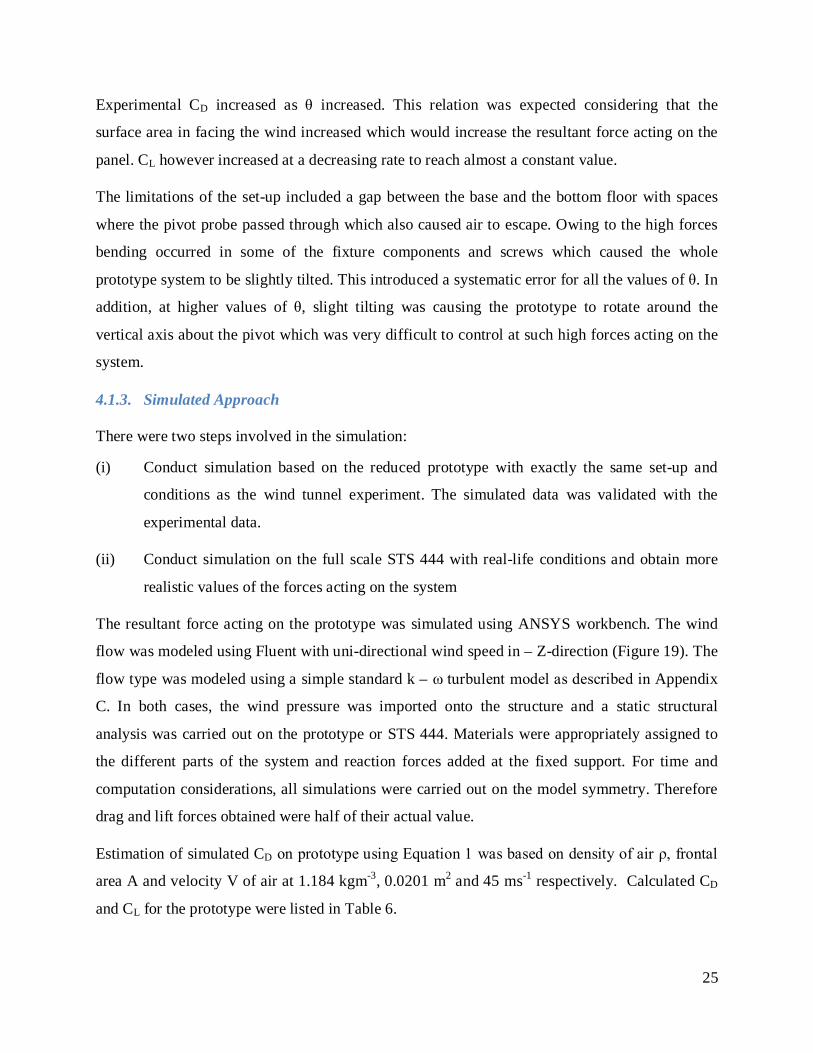
flow was modeled using Fluent with uni-directional wind speed in – Z-direction (Figure 19). The
flow type was modeled using a simple standard k – ω turbulent model as described in Appendix
C. In both cases, the wind pressure was imported onto the structure and a static structural
analysis was carried out on the prototype or STS 444. Materials were appropriately assigned to
the different parts of the system and reaction forces added at the fixed support. For time and
computation considerations, all simulations were carried out on the model symmetry. Therefore
drag and lift forces obtained were half of their actual value.
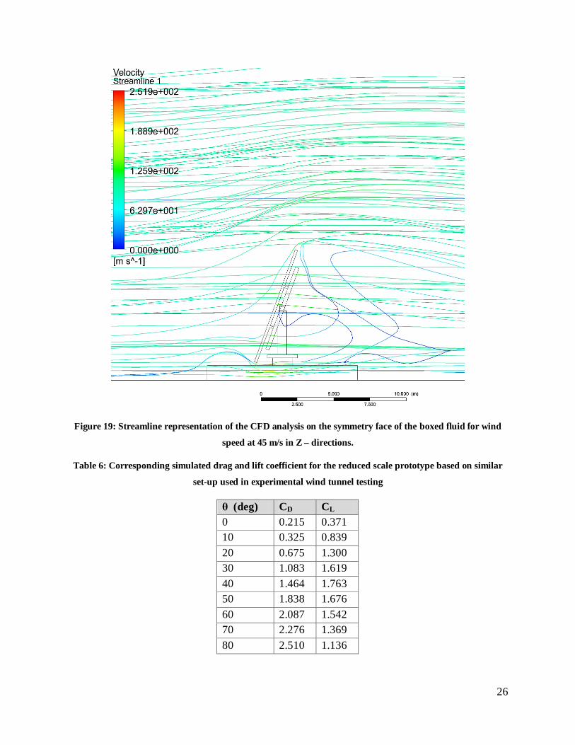
Estimation of simulated CD on prototype using Equation 1 was based on density of air ρ, frontal
area A and velocity V of air at 1.184 kgm-3, 0.0201 m2 and 45 ms-1 respectively. Calculated CD
and CL for the prototype were listed in Table 6.
26
Figure 19: Streamline representation of the CFD analysis on the symmetry face of the boxed fluid for wind
speed at 45 m/s in Z – directions.
Table 6: Corresponding simulated drag and lift coefficient for the reduced scale prototype based on similar
set-up used in experimental wind tunnel testing
θ (deg) CD CL 0 0.215 0.371 10 0.325 0.839 20 0.675 1.300 30 1.083 1.619 40 1.464 1.763 50 1.838 1.676 60 2.087 1.542 70 2.276 1.369 80 2.510 1.136
27
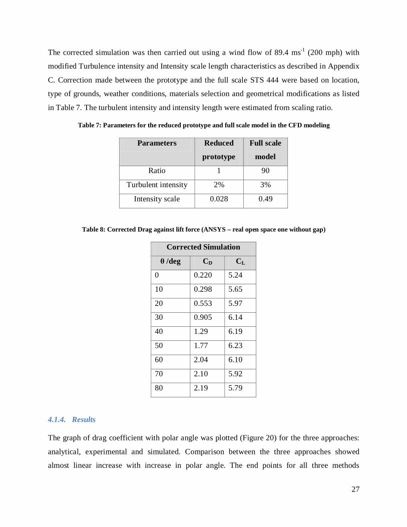
The corrected simulation was then carried out using a wind flow of 89.4 ms-1 (200 mph) with
modified Turbulence intensity and Intensity scale length characteristics as described in Appendix
C. Correction made between the prototype and the full scale STS 444 were based on location,
type of grounds, weather conditions, materials selection and geometrical modifications as listed
in Table 7. The turbulent intensity and intensity length were estimated from scaling ratio.
Table 7: Parameters for the reduced prototype and full scale model in the CFD modeling
Parameters Reduced
prototype
Full scale
model
Ratio 1 90
Turbulent intensity 2% 3%
Intensity scale 0.028 0.49
Table 8: Corrected Drag against lift force (ANSYS – real open space one without gap)
Corrected Simulation
θ /deg CD CL
0 0.220 5.24
10 0.298 5.65
20 0.553 5.97
30 0.905 6.14
40 1.29 6.19
50 1.77 6.23
60 2.04 6.10
70 2.10 5.92
80 2.19 5.79
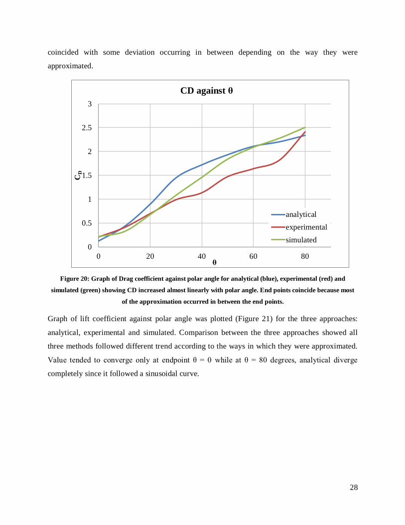
4.1.4. Results
The graph of drag coefficient with polar angle was plotted (Figure 20) for the three approaches:
analytical, experimental and simulated. Comparison between the three approaches showed
almost linear increase with increase in polar angle. The end points for all three methods
28
coincided with some deviation occurring in between depending on the way they were
approximated.
Figure 20: Graph of Drag coefficient against polar angle for analytical (blue), experimental (red) and
simulated (green) showing CD increased almost linearly with polar angle. End points coincide because most
of the approximation occurred in between the end points.
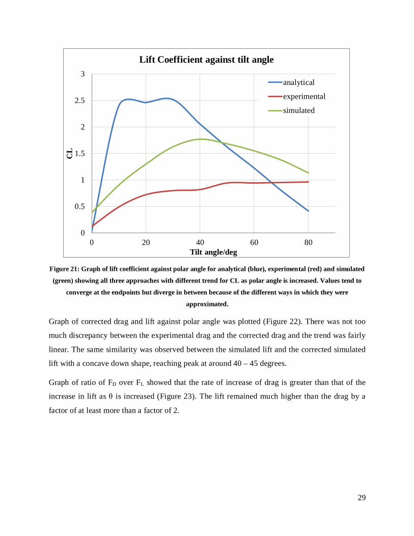
Graph of lift coefficient against polar angle was plotted (Figure 21) for the three approaches:
analytical, experimental and simulated. Comparison between the three approaches showed all
three methods followed different trend according to the ways in which they were approximated.
Value tended to converge only at endpoint θ = 0 while at θ = 80 degrees, analytical diverge
completely since it followed a sinusoidal curve.
0
0.5
1
1.5
2
2.5
3
0 20 40 60 80
CD
θ
CD against θ
analyticalexperimentalsimulated
29
Figure 21: Graph of lift coefficient against polar angle for analytical (blue), experimental (red) and simulated
(green) showing all three approaches with different trend for CL as polar angle is increased. Values tend to
converge at the endpoints but diverge in between because of the different ways in which they were
approximated.
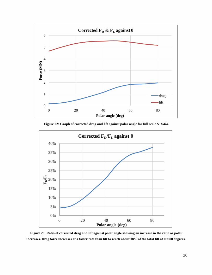
Graph of corrected drag and lift against polar angle was plotted (Figure 22). There was not too
much discrepancy between the experimental drag and the corrected drag and the trend was fairly
linear. The same similarity was observed between the simulated lift and the corrected simulated
lift with a concave down shape, reaching peak at around 40 – 45 degrees.
Graph of ratio of FD over FL showed that the rate of increase of drag is greater than that of the
increase in lift as θ is increased (Figure 23). The lift remained much higher than the drag by a
factor of at least more than a factor of 2.
0
0.5
1
1.5
2
2.5
3
0 20 40 60 80
CL
Tilt angle/deg
Lift Coefficient against tilt angle
analytical
experimental
simulated
30
Figure 22: Graph of corrected drag and lift against polar angle for full scale STS444
Figure 23: Ratio of corrected drag and lift against polar angle showing an increase in the ratio as polar
increases. Drag force increases at a faster rate than lift to reach about 38% of the total lift at θ = 80 degrees.
0
1
2
3
4
5
6
0 20 40 60 80
Forc
e (M
N)
Polar angle (deg)
Corrected FD & FL against θ
drag
lift
0%
5%
10%
15%
20%
25%
30%
35%
40%
0 20 40 60 80
F D/F
L
Polar angle (deg)
Corrected FD/FL against θ

31
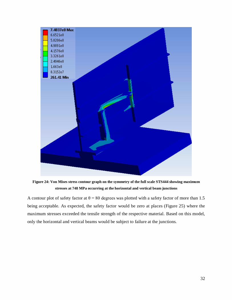
Maximum Von mises stresses (Figure 24) were applied on the simulated system with the
appropriate material assigned to the different parts: concrete to the base, steel to the frame and
aluminum to the panel. Maximum stresses were observed to occur on the steel beams at the
horizontal and vertical beam junctions. Maximum stresses for different polar angles were listed
in Table 9 and followed an increasing trend as polar angle was increase. For a tensile strength of
250 MPa for steel, all the maximum stresses exceed this value by far which indicated failure of
the beams at those locations of maximum stresses.
Table 9: Maximum Von Mises stress based on different polar angles occurring mostly on the horizontal and
vertical beams
θ (deg) Max stress (MPa)
0 266
10 504
20 623
30 707
40 780
50 799
60 755
70 881
80 748
32
Figure 24: Von Mises stress contour graph on the symmetry of the full scale STS444 showing maximum
stresses at 748 MPa occurring at the horizontal and vertical beam junctions
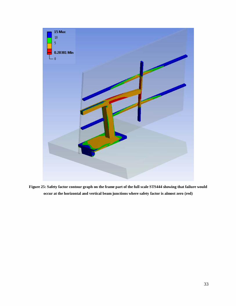
A contour plot of safety factor at θ = 80 degrees was plotted with a safety factor of more than 1.5
being acceptable. As expected, the safety factor would be zero at places (Figure 25) where the
maximum stresses exceeded the tensile strength of the respective material. Based on this model,
only the horizontal and vertical beams would be subject to failure at the junctions.
33
Figure 25: Safety factor contour graph on the frame part of the full scale STS444 showing that failure would
occur at the horizontal and vertical beam junctions where safety factor is almost zero (red)

34
4.1.5. Discussion
Results showed that drag coefficient was directly proportional to polar angle. This was expected
since as angle was increased, the surface in contact with the wind increased which increased
resistance of flow opposing the wind load. From Equation 1, CD is directly proportional to drag
for constant variables. This expected trend was confirmed by all three approaches with deviation
observed in between the endpoints. At the endpoints, the surface areas in contact with the wind
are clear-cut and it is easier to approximate without introducing too much error. At 80 degrees
for example, the panel consisted of mostly two rectangular shapes: the base and the panel as seen
from the frontal area which introduced minimum error in the analytical approach. Whereas in
between the endpoints, the analytical approach for example assumed the flow to be blocked
completely by the surfaces lying in the path of the horizontal wind flow. This caused an
overestimation of the drag. In both the experimental and simulated however, the flow continued
past the panel as would be expected to happen in reality. In addition the shapes of the parts
contributed significantly in estimating the analytical drag coefficient for the system and these
shapes have been in turn simplified to determine their corresponding individual drag coefficient
from textbooks 15. This is why the analytical drag was much higher than the simulated and
experimental drag in between the endpoints (Figure 20). The maximum deviation in the values
between the three approaches was + 40% approximately.
Consider the resultant force as the force perpendicular to the panel surface. The horizontal and
vertical components would then be the drag and lift. When θ = 0, the force perpendicular to the
panel surface is at its minimum so that the lift which will be almost in the same direction as the
resultant force would be at its minimum. As θ is increased, the resultant force acting on the panel
would increase and so will the vertical component which is the lift. At θ = 45 degrees, the
resultant force is at its maximum. As θ is increase, the vertical component will decrease again
but not to zero since the panel is never at 90 degrees. The parabolic trend for the lift therefore
would be expected to be concave down.
Lift coefficients for all three approaches yielded very diverse trends and values. The general
trend was an increase in CL as θ increased with inconclusive trend towards the end when θ was at
a maximum. The analytical approach for example was bound to introduce significant
discrepancies since it was calculated from the sinusoidal component of the drag. The analytical
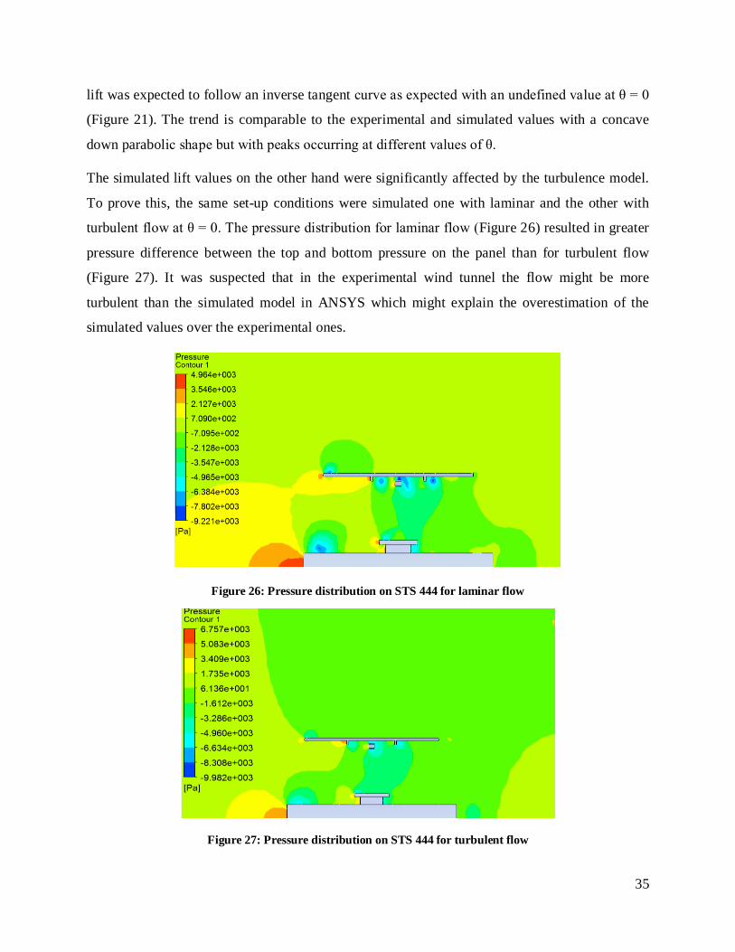
35
lift was expected to follow an inverse tangent curve as expected with an undefined value at θ = 0
(Figure 21). The trend is comparable to the experimental and simulated values with a concave
down parabolic shape but with peaks occurring at different values of θ.
The simulated lift values on the other hand were significantly affected by the turbulence model.
To prove this, the same set-up conditions were simulated one with laminar and the other with
turbulent flow at θ = 0. The pressure distribution for laminar flow (Figure 26) resulted in greater
pressure difference between the top and bottom pressure on the panel than for turbulent flow
(Figure 27). It was suspected that in the experimental wind tunnel the flow might be more
turbulent than the simulated model in ANSYS which might explain the overestimation of the
simulated values over the experimental ones.
Figure 26: Pressure distribution on STS 444 for laminar flow
Figure 27: Pressure distribution on STS 444 for turbulent flow
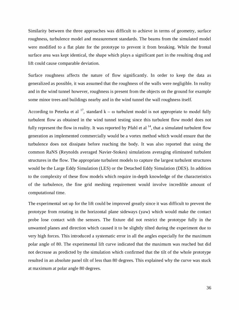
36
Similarity between the three approaches was difficult to achieve in terms of geometry, surface
roughness, turbulence model and measurement standards. The beams from the simulated model
were modified to a flat plate for the prototype to prevent it from breaking. While the frontal
surface area was kept identical, the shape which plays a significant part in the resulting drag and
lift could cause comparable deviation.
Surface roughness affects the nature of flow significantly. In order to keep the data as
generalized as possible, it was assumed that the roughness of the walls were negligible. In reality
and in the wind tunnel however, roughness is present from the objects on the ground for example
some minor trees and buildings nearby and in the wind tunnel the wall roughness itself.
According to Peterka et al 17, standard k – ω turbulent model is not appropriate to model fully
turbulent flow as obtained in the wind tunnel testing since this turbulent flow model does not
fully represent the flow in reality. It was reported by Pfahl et al 14, that a simulated turbulent flow
generation as implemented commercially would be a vortex method which would ensure that the
turbulence does not dissipate before reaching the body. It was also reported that using the
common RaNS (Reynolds averaged Navier-Stokes) simulations averaging eliminated turbulent
structures in the flow. The appropriate turbulent models to capture the largest turbulent structures
would be the Large Eddy Simulation (LES) or the Detached Eddy Simulation (DES). In addition
to the complexity of these flow models which require in-depth knowledge of the characteristics
of the turbulence, the fine grid meshing requirement would involve incredible amount of
computational time.
The experimental set up for the lift could be improved greatly since it was difficult to prevent the
prototype from rotating in the horizontal plane sideways (yaw) which would make the contact
probe lose contact with the sensors. The fixture did not restrict the prototype fully in the
unwanted planes and direction which caused it to be slightly tilted during the experiment due to
very high forces. This introduced a systematic error in all the angles especially for the maximum
polar angle of 80. The experimental lift curve indicated that the maximum was reached but did
not decrease as predicted by the simulation which confirmed that the tilt of the whole prototype
resulted in an absolute panel tilt of less than 80 degrees. This explained why the curve was stuck
at maximum at polar angle 80 degrees.

37
Other sources of error included bending in the fixture and prototype frame support, human error
and other measurement inaccuracies and limitations. The fluctuations of the force sensor
readings were significant at times due to resonance and values were approximated by taking the
mean over a large range of values. The right way would have been to solve the equation of
motion for the forced vibration problem and find the appropriate force however this was left for
future work. Some hysteresis was observed in the measurements since the vibration caused the
pivot arm to shift from its original place.
The correction carried out on the simulated STS 444 was modeled such that it was assumed the
ground was a barren land with almost no obstacles considering that the possible location for the
installations of the STS 444 might be in brownfield lands. Turbulent intensity for the equivalent
simulation of the full-scale model in a full-scale wind tunnel was calculated at 1.46% in
Appendix B. However, the turbulent intensity was reported to be 17% based on typical
surroundings of locations of solar trackers (mostly barren land with scarce trees and buildings)
for an effective surface roughness of 0.03m 17.
Failure at the horizontal and vertical frame beams junctions are only based on the geometry and
size of the beams as modeled. Since information was not disclosed as to the design of those
beams, it can only be recommended that with a cross sectional area of about 0.36 m by 0.36 m
for the horizontal beams and only 0.25 m by 0.13 m for the vertical beams, they would fail at the
junctions. Cross support beams should solve this problem with modification as to the shape of
the beams to reinforced metal I-beams.
4.1.6. Summary
Low reproducibility of wind conditions and profile make it difficult if not impossible to exactly
compare the analytical, simulated and experimental values. The analytical give only a general
value for drag based on generic force coefficient based on simple generalized shape in laminar
flow while for the experimental values, the wind flow was set a certain speed with no knowledge
of the kind of turbulence or other characteristic like vortices. The analytical approach provided
an estimate of the forces in order to calculate the appropriate scaling ratio for the experimental
approach.

38
The first part of the simulation was based entirely on the experimental set-up and was validated
using the experimental values. Once validated, the final realistic forces could then be simulated
with changes to the wind conditions encountered in reality. Therefore the most reliable results
will be the simulated values whereby the wind flow will yield more predictive values that it was
set to simulate. The surface roughness was neglected in the correction which included only wind
blockage, material properties and geometric modifications.
The Von Mises stress analysis showed that the horizontal and vertical beams would fail at the
junctions. Failure depends on geometry and materials assigned to the beams. Future work will
focus on the design and material properties of the beams for a structurally stable system.
4.2. Snow Load Analysis
Part of the autonomy of the STS 444 in withstanding harsh weather conditions will be its ability
to tow snow by rotating the panel. This will be driven by a linear actuator. The speed,
mechanical capacity and electrical power of the linear actuator will depend on the maximum
torque exerted by the snow load. Therefore deriving a snow torque profile to determine
maximum torque exerted by the snow load while sliding off was crucial in selecting the right
linear actuator.
4.2.1. Background
Although snow loads are not as significant as compared to the wind loads, they contribute to
factors that affect the linear actuator kinetics. Modeling of a snow sliding profile was crucial in
finding the time taken for the snow to be completely stowed and the maximum polar angle
required. The snow sliding profile was also very important in finding the torque applied to the
linear actuator shaft by the sliding snow.
It was thought that the sliding snow could be compared to a mini-avalanche effect whereby after
a triggering effect, the snow would usually accelerate rapidly and the amount of snow sliding
would increase exponentially. The equilibrium slope angle of a loose particulate dry snow on a
slope 18 can be approximated by Equation 5 where α is the angle of inclination of the snow
surface and φ is the internal friction angle.
𝛼 = 𝜑 (5)
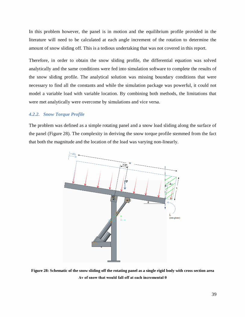
39
In this problem however, the panel is in motion and the equilibrium profile provided in the
literature will need to be calculated at each angle increment of the rotation to determine the
amount of snow sliding off. This is a tedious undertaking that was not covered in this report.
Therefore, in order to obtain the snow sliding profile, the differential equation was solved
analytically and the same conditions were fed into simulation software to complete the results of
the snow sliding profile. The analytical solution was missing boundary conditions that were
necessary to find all the constants and while the simulation package was powerful, it could not
model a variable load with variable location. By combining both methods, the limitations that
were met analytically were overcome by simulations and vice versa.
4.2.2. Snow Torque Profile
The problem was defined as a simple rotating panel and a snow load sliding along the surface of
the panel (Figure 28). The complexity in deriving the snow torque profile stemmed from the fact
that both the magnitude and the location of the load was varying non-linearly.
Figure 28: Schematic of the snow sliding off the rotating panel as a single rigid body with cross section area
Av of snow that would fall off at each incremental θ

40
The list of the variables used to derive the differential equation of motion of the system is given
in Table 10.
Table 10: Terms and definitions of the variables used to derive the differential equation of the snow sliding
torque profile.
Terms Definition
w Width of the panel and snow part
x Height of the snow part
L Length of the panel
A Cross-sectional area of snow (A = wx)
Av Cross-sectional area of snow removed (hatched area)
m Mass of the snow
θ Tilt angle of panel
r(θ) Separation distance between edge of snow part and panel edge (function of θ)
The first part of the derivation consisted of determining the differential equation that governed
the sliding of the snow onto the panel. The differential equation defined by Equation 5 was
solved for r(θ) as derived in Appendix G where µk is the dynamic coefficient of friction.
+ 2𝜇𝑘 − 𝑟2 = 𝑔𝑠𝑖𝑛𝜃 − 𝜇𝑘𝑔𝑐𝑜𝑠𝜃 (6)
The solution to the differential equation was given by Equation 7.
𝑟 = 𝐶1𝑟1 + 𝐶2𝑟2 + 𝑈𝑟1 + 𝑉𝑟2 (7)
where
𝐶1 ,𝐶2 = 𝑐𝑜𝑛𝑠𝑡𝑎𝑛𝑡𝑠
𝑟1 = 𝑒−𝜔(𝜇𝑘+𝐴)𝑡
𝑟2 = 𝑒−𝜔(𝜇𝑘−𝐴)𝑡
𝑈 =−𝑔(𝜇𝑘 + 𝐴)𝑒(𝜇𝑘+𝐴)𝜃
2𝜔𝐴[𝜔2(𝜇𝑘 + 𝐴)2 + 1][𝑠𝑖𝑛𝜃 −
𝑐𝑜𝑠𝜃𝜔(𝜇𝑘 + 𝐴) − 𝜇𝑘𝑐𝑜𝑠𝜃 −
𝜇𝑘𝑠𝑖𝑛𝜃𝜔(𝜇𝑘 + 𝐴)]
𝑉 =𝑔(𝜇𝑘 − 𝐴)𝑒(𝜇𝑘−𝐴)𝜃
2𝜔𝐴[𝜔2(𝜇𝑘 − 𝐴)2 + 1][𝑠𝑖𝑛𝜃 −
𝑐𝑜𝑠𝜃𝜔(𝜇𝑘 − 𝐴) − 𝜇𝑘𝑐𝑜𝑠𝜃 −
𝜇𝑘𝑠𝑖𝑛𝜃𝜔(𝜇𝑘 − 𝐴)]
𝜃 = 𝜔𝑡
41
𝐴 = (𝜇𝑘2 + 1)
The initial condition was obtained by finding the angle at which the static snow was just about to
slip which was given by Equation 8 where µs is the static coefficient of friction. The relation was
derived in Appendix G.
𝑔𝑠𝑖𝑛𝜃 + 𝜇𝑠𝑔𝑐𝑜𝑠𝜃 = −𝑟 (8)
For an arbitrary value of the angular velocity ω at 0.1 rad/s, the angle of slip was just about 10.5
degrees for r(θ) = 0. However another set of boundary conditions were needed to determine the
values of the constants C1 and C2.
This limitation was overcome by simulating the sliding based on the initial conditions and the
values of µs and µk to obtain a set of boundary conditions.
The second part of the derivation consisted of determining the magnitude of the load. It was
assumed that incremental area Av (Figure 28) would represent the decrease of load with θ. Other
approximation of the snow leaving the panel would result in higher or lower estimation than
what was used here. The variation in the magnitude of the load was given by Equation 9 as
derived in Appendix G.
𝑊𝑠(𝜃) = 𝜌𝑔𝐿 𝑥𝑤 − 𝑟(𝜃)𝑥 +𝑥2𝑡𝑎𝑛𝜃 (9)
Hence the torque exerted by the snow at the pivot point O was defined by Equation 10
𝑇𝑠 =12𝑊𝑠(𝜃)𝑟(𝜃) (10)
Assuming no power is lost, the force exerted axially on the linear actuator bearings would then
be given by Equation 11. For small angles of θ, ω can be approximated as constant.
𝐹(𝜃) =𝑇(𝜃)𝜔(𝜃)
𝑣 (11)
4.2.2.1. Model parts and Assembly
Most simulate package required prior knowledge of the snow sliding profile which needed to be
fed to the simulation set-up which was what was sought after. The problem in this analysis being
more of deductive problem than inductive required over-simplification of the snow sliding

42
profile. Therefore assumptions were needed for the snow unloading simulation with detailed
simulation parameters given in Appendix G:
i. Snow was assumed to be a discrete load and was modeled as a part to capture both the change in load direction and load magnitude.
ii. Snow was taken as fresh new snow 18 with a density of 50 – 70 kgm-3
iii. Gravity was the only external force acting on the system
iv. Static and dynamic friction of snow on PV panel was approximated as 0.1 and 0.03 19
respectively
v. All other connections and contact surfaces were assumed to be frictionless
vi. Linear actuator was assigned a constant speed
The problem was having the location of the applied load change as well as the magnitude of the
applied load. While the change in magnitude was easy enough to be set up, the change in
direction of the force could only be simulated by modeling the snow as a part interacting with the
mechanism in motion. The snow was modeled as a flat rectangular body to simplify the
mechanism analysis set-up.
The solar tracker system subassembly consisted of 4 parts: panel, linear actuator motor housing,
linear actuator shaft and frame support. The frame (Figure 29) was assembled with a rigid
connection while the linear actuator motor housing (Figure 29) was constraint with a pin
connection at the axis of rotation with the frame support. The linear actuator shaft (Figure 29)
was constraint with both a slider connection and a bearing connection with the linear actuator
motor housing and PV panel respectively. The snow part (Figure 29) was constraint with a slider
connection between the snow surface and the panel surface.
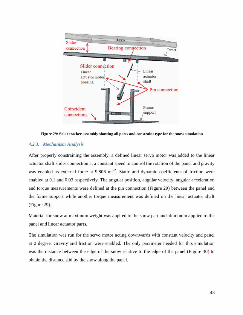
43
Figure 29: Solar tracker assembly showing all parts and constraint type for the snow simulation
4.2.3. Mechanism Analysis
After properly constraining the assembly, a defined linear servo motor was added to the linear
actuator shaft slider connection at a constant speed to control the rotation of the panel and gravity
was enabled as external force at 9.806 ms-2. Static and dynamic coefficients of friction were
enabled at 0.1 and 0.03 respectively. The angular position, angular velocity, angular acceleration
and torque measurements were defined at the pin connection (Figure 29) between the panel and
the frame support while another torque measurement was defined on the linear actuator shaft
(Figure 29).
Material for snow at maximum weight was applied to the snow part and aluminum applied to the
panel and linear actuator parts.
The simulation was run for the servo motor acting downwards with constant velocity and panel
at 0 degree. Gravity and friction were enabled. The only parameter needed for this simulation
was the distance between the edge of the snow relative to the edge of the panel (Figure 30) to
obtain the distance slid by the snow along the panel.
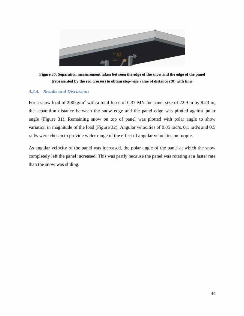
44
Figure 30: Separation measurement taken between the edge of the snow and the edge of the panel
(represented by the red crosses) to obtain step-wise value of distance r(θ) with time
4.2.4. Results and Discussion
For a snow load of 200kg/m2 with a total force of 0.37 MN for panel size of 22.9 m by 8.23 m,
the separation distance between the snow edge and the panel edge was plotted against polar
angle (Figure 31). Remaining snow on top of panel was plotted with polar angle to show
variation in magnitude of the load (Figure 32). Angular velocities of 0.05 rad/s, 0.1 rad/s and 0.5
rad/s were chosen to provide wider range of the effect of angular velocities on torque.
As angular velocity of the panel was increased, the polar angle of the panel at which the snow
completely left the panel increased. This was partly because the panel was rotating at a faster rate
than the snow was sliding.
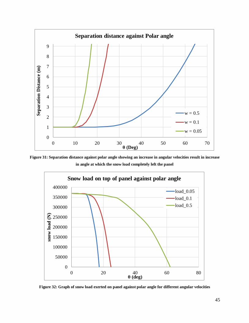
45
Figure 31: Separation distance against polar angle showing an increase in angular velocities result in increase
in angle at which the snow load completely left the panel
Figure 32: Graph of snow load exerted on panel against polar angle for different angular velocities
0
1
2
3
4
5
6
7
8
9
0 10 20 30 40 50 60 70
Sepa
ratio
n D
ista
nce
(m)
θ (Deg)
Separation distance against Polar angle
w = 0.5
w = 0.1
w = 0.05
0
50000
100000
150000
200000
250000
300000
350000
400000
0 20 40 60 80
snow
load
(N)
θ (deg)
Snow load on top of panel against polar angle
load_0.05load_0.1load_0.5
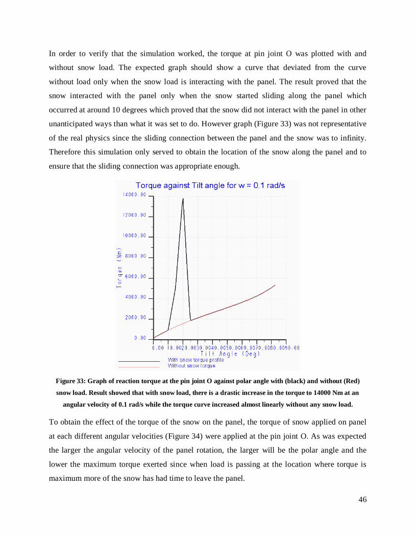
46
In order to verify that the simulation worked, the torque at pin joint O was plotted with and
without snow load. The expected graph should show a curve that deviated from the curve
without load only when the snow load is interacting with the panel. The result proved that the
snow interacted with the panel only when the snow started sliding along the panel which
occurred at around 10 degrees which proved that the snow did not interact with the panel in other
unanticipated ways than what it was set to do. However graph (Figure 33) was not representative
of the real physics since the sliding connection between the panel and the snow was to infinity.
Therefore this simulation only served to obtain the location of the snow along the panel and to
ensure that the sliding connection was appropriate enough.
Figure 33: Graph of reaction torque at the pin joint O against polar angle with (black) and without (Red)
snow load. Result showed that with snow load, there is a drastic increase in the torque to 14000 Nm at an
angular velocity of 0.1 rad/s while the torque curve increased almost linearly without any snow load.
To obtain the effect of the torque of the snow on the panel, the torque of snow applied on panel
at each different angular velocities (Figure 34) were applied at the pin joint O. As was expected
the larger the angular velocity of the panel rotation, the larger will be the polar angle and the
lower the maximum torque exerted since when load is passing at the location where torque is
maximum more of the snow has had time to leave the panel.
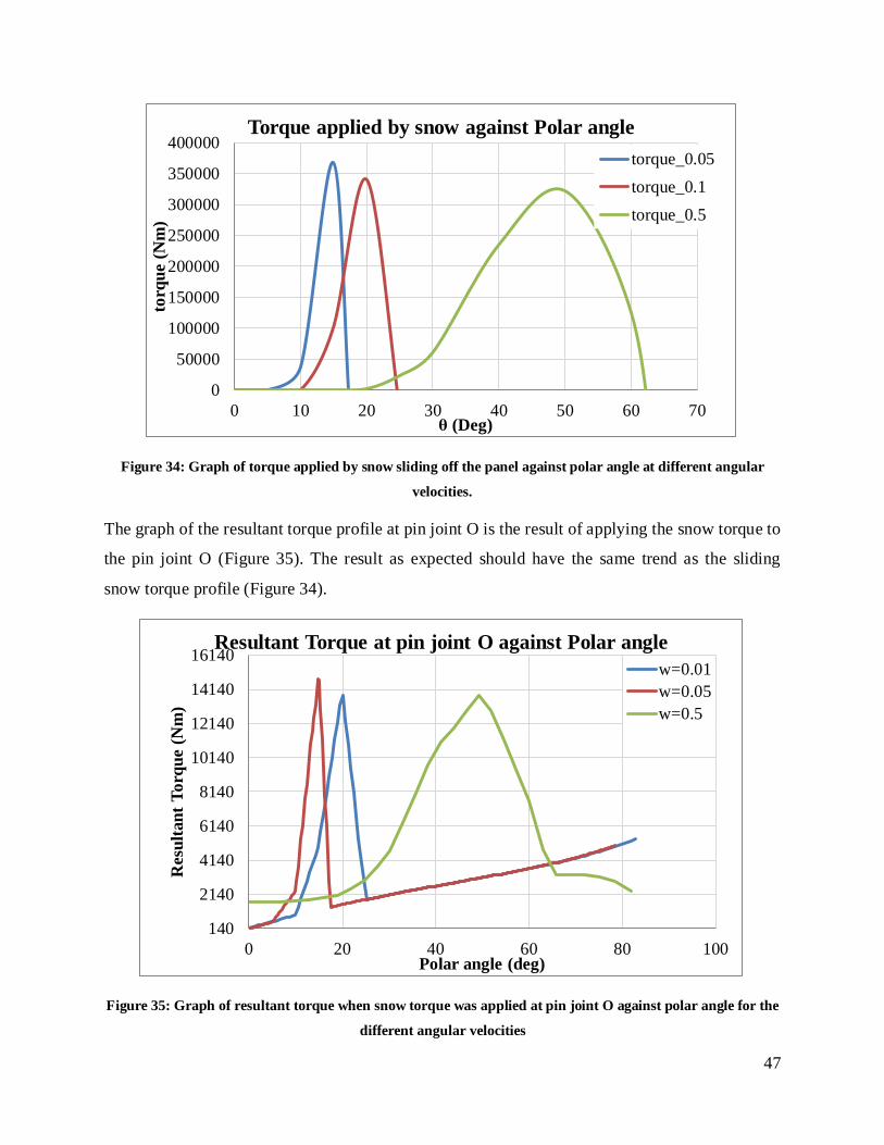
47
Figure 34: Graph of torque applied by snow sliding off the panel against polar angle at different angular
velocities.
The graph of the resultant torque profile at pin joint O is the result of applying the snow torque to
the pin joint O (Figure 35). The result as expected should have the same trend as the sliding
snow torque profile (Figure 34).
Figure 35: Graph of resultant torque when snow torque was applied at pin joint O against polar angle for the
different angular velocities
0
50000
100000
150000
200000
250000
300000
350000
400000
0 10 20 30 40 50 60 70
torq
ue (N
m)
θ (Deg)
Torque applied by snow against Polar angle torque_0.05torque_0.1torque_0.5
140
2140
4140
6140
8140
10140
12140
14140
16140
0 20 40 60 80 100
Res
ulta
nt T
orqu
e (N
m)
Polar angle (deg)
Resultant Torque at pin joint O against Polar angle w=0.01w=0.05w=0.5
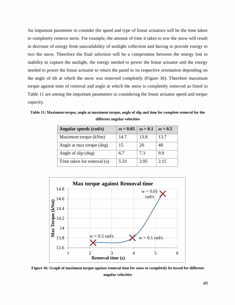
48
An important parameter to consider the speed and type of linear actuators will be the time taken
to completely remove snow. For example, the amount of time it takes to tow the snow will result
in decrease of energy from unavailability of sunlight collection and having to provide energy to
two the snow. Therefore the final selection will be a compromise between the energy lost in
inability to capture the sunlight, the energy needed to power the linear actuator and the energy
needed to power the linear actuator to return the panel to its respective orientation depending on
the angle of tilt at which the snow was removed completely (Figure 36). Therefore maximum
torque against time of removal and angle at which the snow is completely removed as listed in
Table 11 are among the important parameters in considering the linear actuator speed and torque
capacity.
Table 11: Maximum torque, angle at maximum torque, angle of slip and time for complete removal for the
different angular velocities
Angular speeds (rad/s) ω = 0.05 ω = 0.1 ω = 0.5
Maximum torque (kNm) 14.7 13.8 13.7
Angle at max torque (deg) 15 20 48
Angle of slip (deg) 6.7 7.3 9.9
Time taken for removal (s) 5.33 3.95 2.15
Figure 36: Graph of maximum torque against removal time for snow to completely be towed for different
angular velocities
w = 0.01 rad/s
w = 0.1 rad/s w = 0.5 rad/s
13.6
13.8
14
14.2
14.4
14.6
14.8
1 2 3 4 5 6
Max
Tor
que
(kN
m)
Removal time (s)
Max torque against Removal time

49
It is important to note that the simulated results were based on the specific conditions such as
constant speed driving the linear actuator shaft, the mass of a discrete rigid body, coefficients of
friction, initial position of panel and snow load and shape of the snow load.
4.2.5. Summary
The sliding snow torque profile was based on numerous assumptions that were made as general
as possible. The maximum torque was found to be 14.7 kNm approximately for an angular
velocity of 0.01 rad/s of the panel rotation and for snow load at 200 kg/m2. The time for
complete removal at that angular velocity was around 5 – 6 seconds based on a coefficient of
kinetic and static friction of 0.03 and 0.1 respectively. It was also assumed all other joints were
frictionless and that no other frictional sources were acting on the system for example wind drag.
Higher angular velocities of the panel were also analyzed which yielded lower maximum torque
and lower removal time but higher angle of rotation. This introduced the concept of cost
performance whereby the cost of the energy lost in rotating the panel a greater angle against
higher torque needed for a smaller displacement requires optimization in order to select the right
speed and capacity for the linear actuator. The economics aspect of the solar tracker is a subject
that would be addressed in future work.
4.3. Conclusions and Recommendations
Results showed that the snow load was not as significant as compared to the wind load by at least
a factor of 10. In addition the wind load can cause a great amount of mechanical damage in the
sense that if in addition to the maximum wind load, the frequency of the wind equaled that of the
mechanism system this will result in resonance.
Therefore the optimization of the beams supporting the panel and the base should be based on
the wind force and stress analyses while the snow load analysis will be mostly geared towards
selecting the right linear actuator. Based on the large amount of drag, the non-ground penetrating
base should be strong enough not to be uprooted while part of the lift will be pushing vertically
down on the solar tracker, this might help in anchoring the base to the ground during wind
storms with wind at 89.4 m/s (200mph) .
It was recommended based on the stress analysis of the solar tracker that the horizontal and
vertical beams supporting the panel should be increased and reinforced further to prevent failure

50
and the assumptions used in this report for the snow load analysis was that the solar tracker parts
were negligible in weight as compared to the snow load. For the selection of the linear actuator,
weights of the beams and panel parts need to be included for correctly predicting the maximum
torque of the snow.
Both the wind and the snow load are critical to optimizing the design of the STS 444. This
project only offered a rough preliminary estimate of the forces acting on the STS 444. Future
work will focus on optimization of in-depth structural design and how parameters such as energy
power to the driving actuators and gears affect the economics of the STS 444 depending on the
speed of the cycles, the amount of tracking, type of tracking and default configurations in
response to critical conditions.

51
5. FUNCTIONAL MODEL
The purpose of the functional model was to demonstrate to FDE’s customers how the large scale
model (STS 444) duel-axis tracker would operate. The first step of realizing the functional model
was to define the design specifications for the model.
5.1. Design Specifications
The design specifications for the functional model were based on the specifications set by the
FDE and additional specifications generated by the team.
1. The functional model should be at most a three-piece assembly that could be disassembled
into the panel, frame support and base
2. A panel with dimensions 1.58m × 0.81m at 16 kg was provided and all other parts should be
designed correspondingly
3. The three disassembled parts should fit within a design envelop of 62 in × 32 in × 12 in
(1.58m × 0.81m × 0.3 m) for storage and transportation
4. The function model should be able to assembled or disassembled within 2 minute and should
be easily transported by one person
5. The total weight must be less than 36 kg (80 lbs.)
6. The panel should be able to rotate a full 360 degrees around the azimuth (vertical) axis
7. The panel should be able to tilt a maximum of 80 degrees with the polar (horizontal) axis
8. The model should be able to demonstrate snow removal simulation, solar tracking up to ±5
degree accuracy, and go into the low-drag mode in windy conditions to reduce drag forces
9. The model should be able to use power from the solar panel during outdoor use or the 110V
AC socket during indoor use
10. The model should contain an internal battery when the two power sources are not available
11. The sensors should respond to external stimuli for wind, snow load and light simulation
12. Parts used should be easily obtained and compatible with all assembly parts used
13. The prototype must be easy to troubleshoot and easily assembled by a trained mechanic
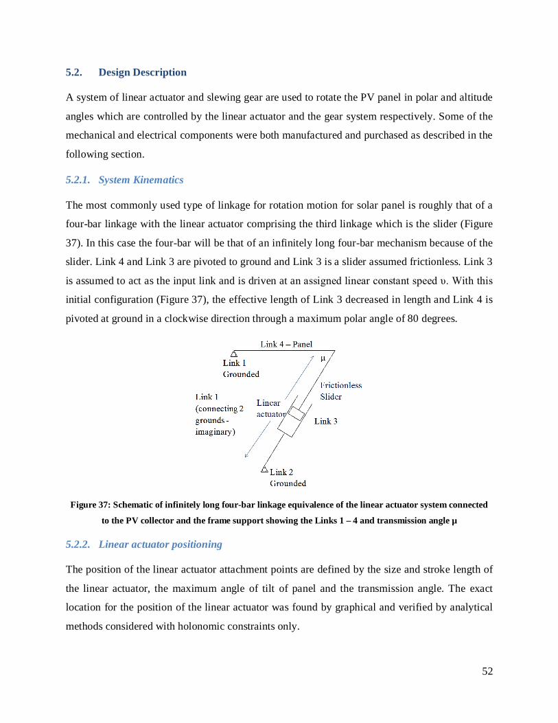
52
5.2. Design Description
A system of linear actuator and slewing gear are used to rotate the PV panel in polar and altitude
angles which are controlled by the linear actuator and the gear system respectively. Some of the
mechanical and electrical components were both manufactured and purchased as described in the
following section.
5.2.1. System Kinematics
The most commonly used type of linkage for rotation motion for solar panel is roughly that of a
four-bar linkage with the linear actuator comprising the third linkage which is the slider (Figure
37). In this case the four-bar will be that of an infinitely long four-bar mechanism because of the
slider. Link 4 and Link 3 are pivoted to ground and Link 3 is a slider assumed frictionless. Link 3
is assumed to act as the input link and is driven at an assigned linear constant speed υ. With this
initial configuration (Figure 37), the effective length of Link 3 decreased in length and Link 4 is
pivoted at ground in a clockwise direction through a maximum polar angle of 80 degrees.
Figure 37: Schematic of infinitely long four-bar linkage equivalence of the linear actuator system connected
to the PV collector and the frame support showing the Links 1 – 4 and transmission angle µ
5.2.2. Linear actuator positioning
The position of the linear actuator attachment points are defined by the size and stroke length of
the linear actuator, the maximum angle of tilt of panel and the transmission angle. The exact
location for the position of the linear actuator was found by graphical and verified by analytical
methods considered with holonomic constraints only.

53
Ideally the linear actuator would be in compression when carrying the highest load, that is, when
the panel is being pushed up from a tilted position to the horizontal position. From a material
engineering point of view, the microvoids and shear bands tend to form in relatively brittle
materials in tension which limit the ability of the material to undergo strain. Although in such a
small scale system as the functional prototype sudden fracture is not likely to cause any damage,
for the much larger STS 444 system, creep may be one of the most critical material behaviors to
anticipate failure. This is why keeping the linear actuator in compression is so important.
Selection of linear actuator
The selection of the linear actuator was a compromise between what was available commercially
and the corresponding sizes, weights, costs and performances. Linear actuators from ServoCity 20
offered a range of different linear actuator that was within the allocated budget. The stroke
lengths for the available linear actuators were listed in Table 12. The cost and the performance
for the different stroke lengths of the chosen linear actuator type were comparable with
maximum velocity of 2 inch/sec (0.05m/s) and a maximum load capacity of 115lbs (512N
approximately).
The limiting conditions were the dimension and mass of the linear actuators: the linear actuator
should have a minimum length that fits into the functional model when fully retracted at least
and the longer the stroke length the heavier the linear actuator will weigh.
Dimensional limitation
The dimensional limitation was the most critical limitation when selecting the linear actuator
based on the dimensions of the solar panel as specified in the design specifications.
Parts were modeled based on available standard parts and materials are available and
dimensional as well as other limitations as will be described in following sections.
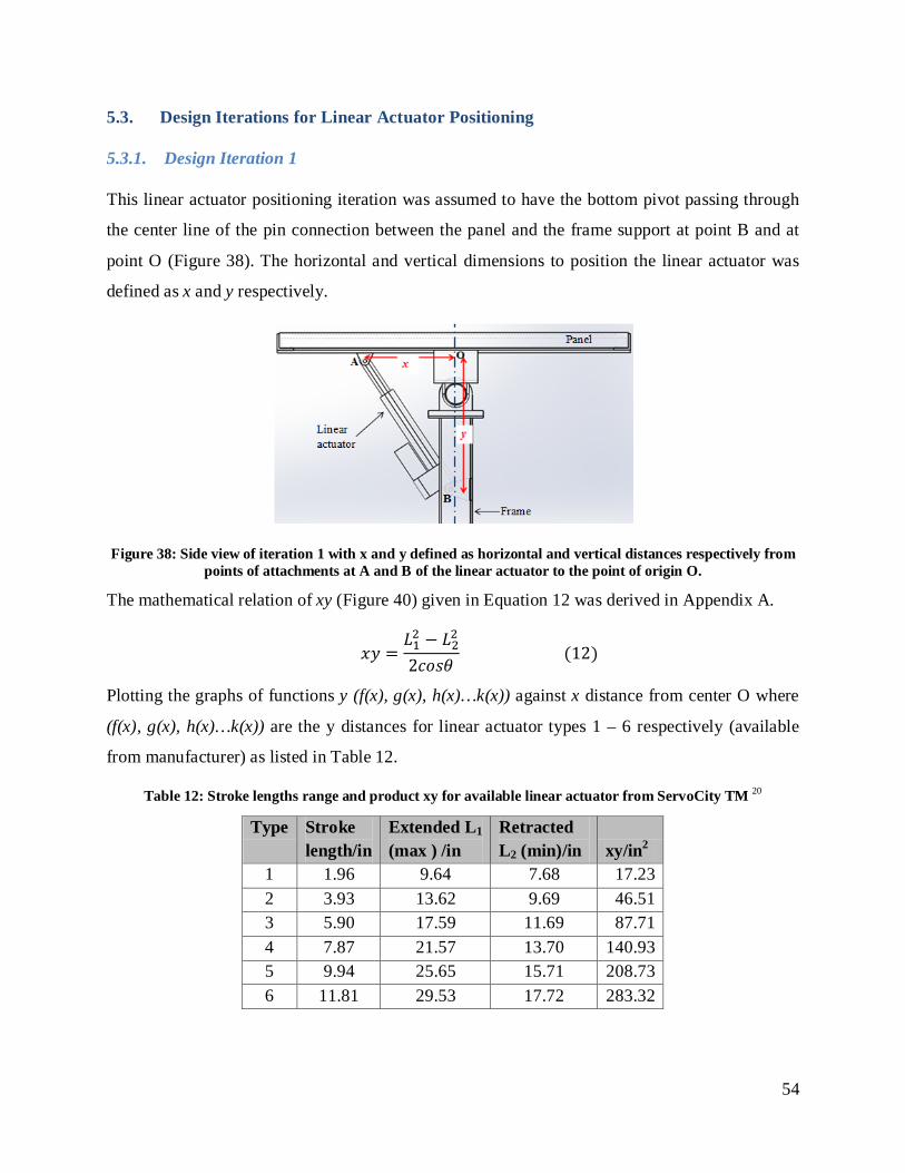
54
5.3. Design Iterations for Linear Actuator Positioning
5.3.1. Design Iteration 1
This linear actuator positioning iteration was assumed to have the bottom pivot passing through
the center line of the pin connection between the panel and the frame support at point B and at
point O (Figure 38). The horizontal and vertical dimensions to position the linear actuator was
defined as x and y respectively.
Figure 38: Side view of iteration 1 with x and y defined as horizontal and vertical distances respectively from points of attachments at A and B of the linear actuator to the point of origin O.
The mathematical relation of xy (Figure 40) given in Equation 12 was derived in Appendix A.
𝑥𝑦 =𝐿12 − 𝐿22
2𝑐𝑜𝑠𝜃 (12)
Plotting the graphs of functions y (f(x), g(x), h(x)…k(x)) against x distance from center O where
(f(x), g(x), h(x)…k(x)) are the y distances for linear actuator types 1 – 6 respectively (available
from manufacturer) as listed in Table 12.
Table 12: Stroke lengths range and product xy for available linear actuator from ServoCity TM 20
Type Stroke length/in
Extended L1 (max ) /in
Retracted L2 (min)/in xy/in2
1 1.96 9.64 7.68 17.23 2 3.93 13.62 9.69 46.51 3 5.90 17.59 11.69 87.71 4 7.87 21.57 13.70 140.93 5 9.94 25.65 15.71 208.73 6 11.81 29.53 17.72 283.32
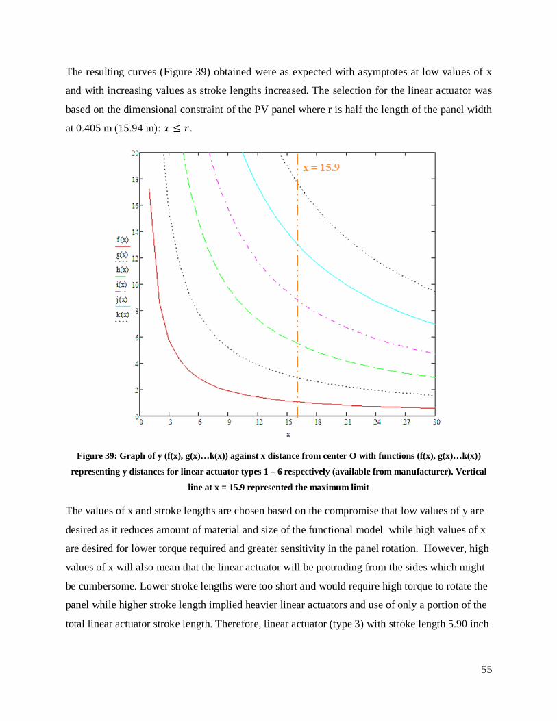
55
The resulting curves (Figure 39) obtained were as expected with asymptotes at low values of x
and with increasing values as stroke lengths increased. The selection for the linear actuator was
based on the dimensional constraint of the PV panel where r is half the length of the panel width
at 0.405 m (15.94 in): 𝑥 ≤ 𝑟.
Figure 39: Graph of y (f(x), g(x)…k(x)) against x distance from center O with functions (f(x), g(x)…k(x))
representing y distances for linear actuator types 1 – 6 respectively (available from manufacturer). Vertical
line at x = 15.9 represented the maximum limit
The values of x and stroke lengths are chosen based on the compromise that low values of y are
desired as it reduces amount of material and size of the functional model while high values of x
are desired for lower torque required and greater sensitivity in the panel rotation. However, high
values of x will also mean that the linear actuator will be protruding from the sides which might
be cumbersome. Lower stroke lengths were too short and would require high torque to rotate the
panel while higher stroke length implied heavier linear actuators and use of only a portion of the
total linear actuator stroke length. Therefore, linear actuator (type 3) with stroke length 5.90 inch

56
was chosen since it was the minimum stroke length to yield reasonable y values (x = 10.69in, y =
13.96in).
The limitations for this design iteration were as followed:
i. The dimension ranges were calculated only at the different extreme positions and
dynamic motions were not taken into consideration
ii. Rotation point was taken at the center of mass of panel when in reality pivot point is
found slightly offset along the vertical axis
iii. Attachment points of linear actuator on panel and beam were taken to be lying right
onto the mid-axis. Optimum position of the attachment points might not be lying on
the vertical and horizontal axes.
Although simple in concept, this iteration failed as it did not satisfy the “maximum polar angle of
the panel at 80 degrees” design specification requirement.
5.3.2. Design Iteration 2
This design iteration addressed the maximum tilt angle of 80 degrees requirement by removing
the constraint for point B (point of attachment between the bottom of the linear actuator and the
frame). In the previous design iteration, B was constraint along center axis of frame passing
through O. A new variable δ (Figure 40) was introduced as the offset distance between O and O’.
Figure 40: Side view of iteration 1 with x and y defined as horizontal and vertical distances respectively from
points of attachments at A and B of the linear actuator to the point of origin O’ and δ as offset distance
between O and O’.
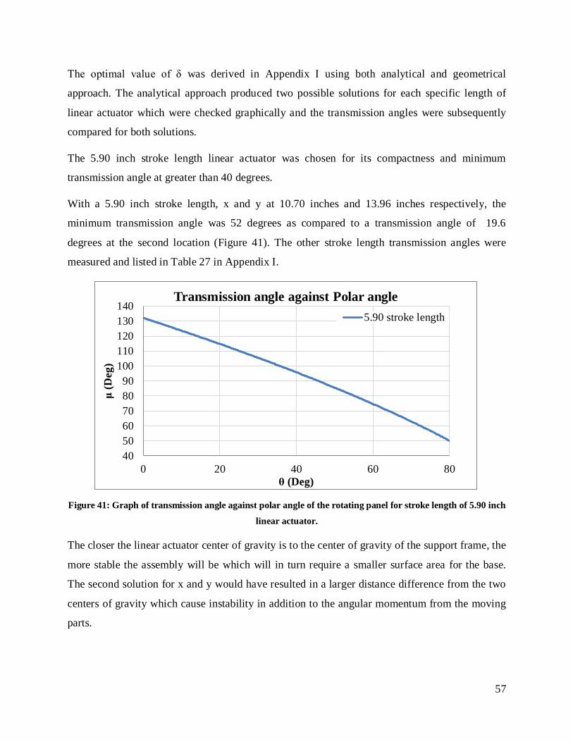
57
The optimal value of δ was derived in Appendix I using both analytical and geometrical
approach. The analytical approach produced two possible solutions for each specific length of
linear actuator which were checked graphically and the transmission angles were subsequently
compared for both solutions.
The 5.90 inch stroke length linear actuator was chosen for its compactness and minimum
transmission angle at greater than 40 degrees.
With a 5.90 inch stroke length, x and y at 10.70 inches and 13.96 inches respectively, the
minimum transmission angle was 52 degrees as compared to a transmission angle of 19.6
degrees at the second location (Figure 41). The other stroke length transmission angles were
measured and listed in Table 27 in Appendix I.
Figure 41: Graph of transmission angle against polar angle of the rotating panel for stroke length of 5.90 inch
linear actuator.
The closer the linear actuator center of gravity is to the center of gravity of the support frame, the
more stable the assembly will be which will in turn require a smaller surface area for the base.
The second solution for x and y would have resulted in a larger distance difference from the two
centers of gravity which cause instability in addition to the angular momentum from the moving
parts.
405060708090
100110120130140
0 20 40 60 80
μ (D
eg)
θ (Deg)
Transmission angle against Polar angle 5.90 stroke length
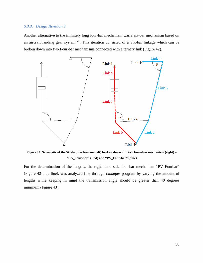
58
5.3.3. Design Iteration 3
Another alternative to the infinitely long four-bar mechanism was a six-bar mechanism based on
an aircraft landing gear system 21. This iteration consisted of a Six-bar linkage which can be
broken down into two Four-bar mechanisms connected with a ternary link (Figure 42).
Figure 42: Schematic of the Six-bar mechanism (left) broken down into two Four-bar mechanism (right) –
“LA_Four-bar” (Red) and “PV_Four-bar” (blue)
For the determination of the lengths, the right hand side four-bar mechanism “PV_Fourbar”
(Figure 42-blue line), was analyzed first through Linkages program by varying the amount of
lengths while keeping in mind the transmission angle should be greater than 40 degrees
minimum (Figure 43).
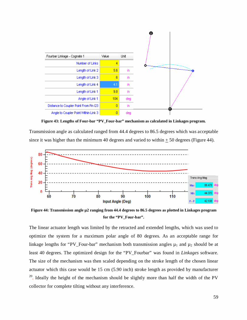
59
Figure 43: Lengths of Four-bar “PV_Four-bar” mechanism as calculated in Linkages program.
Transmission angle as calculated ranged from 44.4 degrees to 86.5 degrees which was acceptable
since it was higher than the minimum 40 degrees and varied to within + 50 degrees (Figure 44).
Figure 44: Transmission angle µ2 ranging from 44.4 degrees to 86.5 degrees as plotted in Linkages program
for the “PV_Four-bar”.
The linear actuator length was limited by the retracted and extended lengths, which was used to
optimize the system for a maximum polar angle of 80 degrees. As an acceptable range for
linkage lengths for “PV_Four-bar” mechanism both transmission angles µ1 and µ2 should be at
least 40 degrees. The optimized design for the “PV_Fourbar” was found in Linkages software.
The size of the mechanism was then scaled depending on the stroke length of the chosen linear
actuator which this case would be 15 cm (5.90 inch) stroke length as provided by manufacturer 20. Ideally the height of the mechanism should be slightly more than half the width of the PV
collector for complete tilting without any interference.

60
Once the model was scaled based on the optimization of the “PV_Fourbar” and the linear
actuator length, the linkages were modeled in CAD (Figure 45). Motion was simulated with a
constant speed of 0.01 m/s for servo motor added to the linear actuator. Measurement of
transmission angle µ1 was then determined during the simulation which yielded 6.6 degrees and
55 degrees approximately at the two extreme positions (Figure 46).
Figure 45: Model of the six-bar mechanism showing the two extreme positions at θ = 0 degrees (left) and θ =
80 degrees (left).
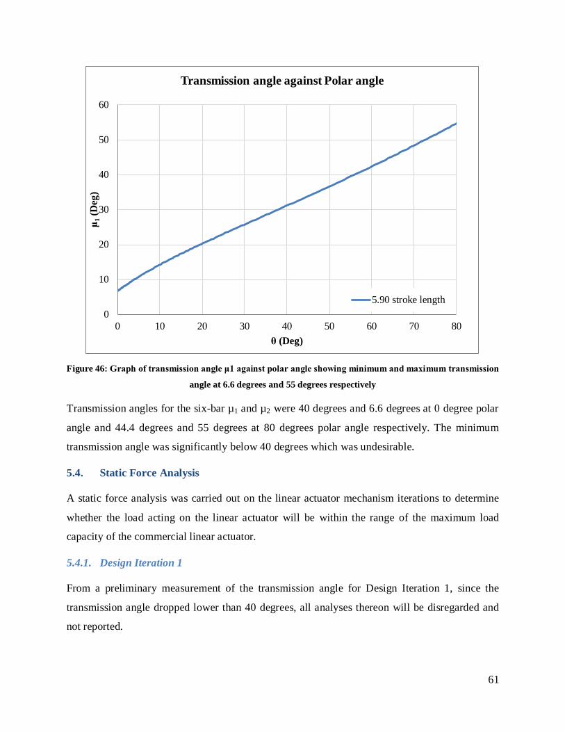
61
Figure 46: Graph of transmission angle μ1 against polar angle showing minimum and maximum transmission
angle at 6.6 degrees and 55 degrees respectively
Transmission angles for the six-bar µ1 and µ2 were 40 degrees and 6.6 degrees at 0 degree polar
angle and 44.4 degrees and 55 degrees at 80 degrees polar angle respectively. The minimum
transmission angle was significantly below 40 degrees which was undesirable.
5.4. Static Force Analysis
A static force analysis was carried out on the linear actuator mechanism iterations to determine
whether the load acting on the linear actuator will be within the range of the maximum load
capacity of the commercial linear actuator.
5.4.1. Design Iteration 1
From a preliminary measurement of the transmission angle for Design Iteration 1, since the
transmission angle dropped lower than 40 degrees, all analyses thereon will be disregarded and
not reported.
0
10
20
30
40
50
60
0 10 20 30 40 50 60 70 80
μ 1 (D
eg)
θ (Deg)
Transmission angle against Polar angle
5.90 stroke length

62
5.4.2. Design iteration 2
Static forces were derived analytically using FDBs as drawn in Appendix J. The parameters used
in the derivation were listed in Table 28 in Appendix J. Maximum static force acting on the
system would occur at different positions depending on the connections as derived in Appendix
J. Reaction static forces at the pin joints where the linear actuator connected to the panel
approximated a maximum of 2.64 N when polar angle was at 0 degrees. Reaction static forces at
the bottom connection of the linear actuator where it connected with the frame support
approximated 12 N at a polar angle of 80 degrees.
5.4.3. Design Iteration 3
A full static analysis of the six-bar mechanism was carried out by simulation. Results showed
that at polar angle of 0 degree the static reaction force was at 2 N approximately while at polar
angle of 80 degrees, the static reaction force was at approximately 157 N (Figure 47).
Figure 47: Static reaction forces at connection between the linear actuator and the panel at 0 degrees (left) and at 80 degrees (right) polar angle were 2 N and 157 N respectively
5.4.4. Selection of linear actuator mechanism
The factors considered in the selection of the mechanism for the linear actuator were
transmission angle, dimensions, number of parts and torque as listed in Table 13.
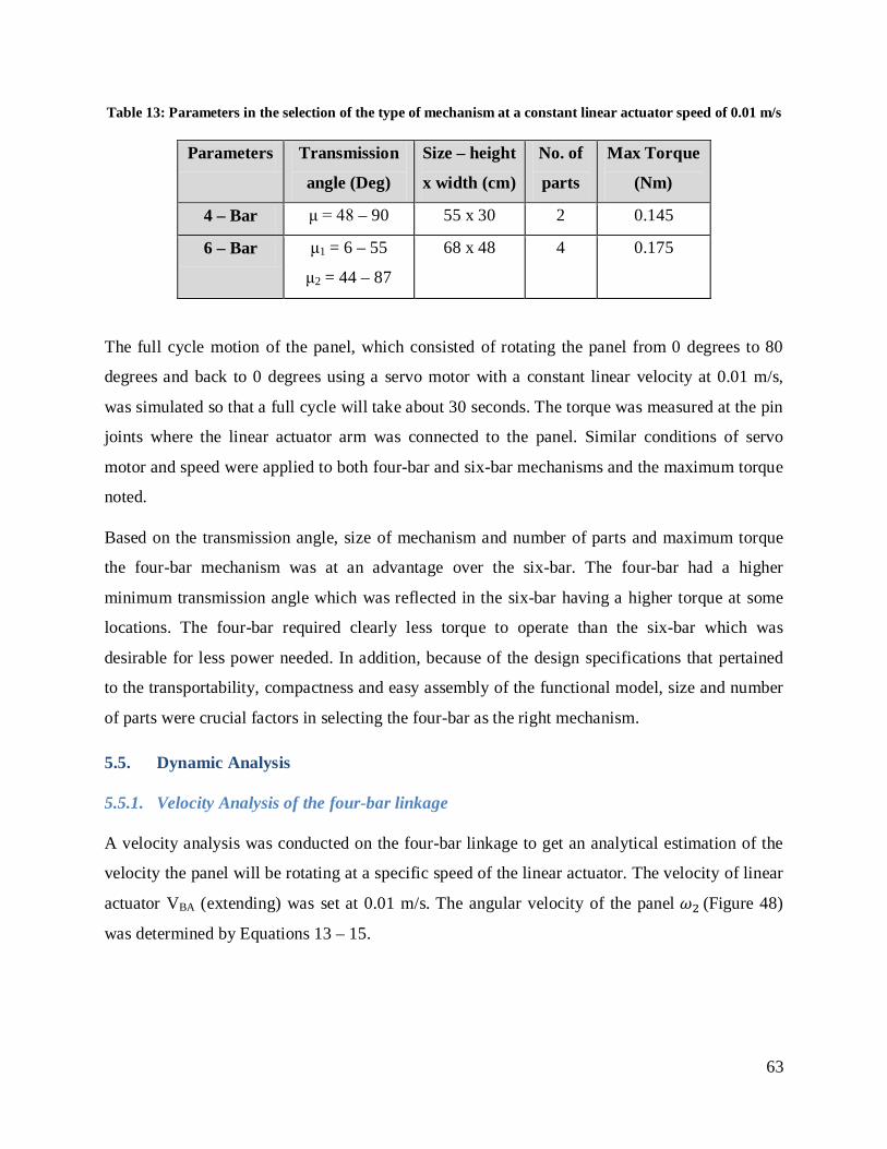
63
Table 13: Parameters in the selection of the type of mechanism at a constant linear actuator speed of 0.01 m/s
Parameters Transmission
angle (Deg)
Size – height
x width (cm)
No. of
parts
Max Torque
(Nm)
4 – Bar μ = 48 – 90 55 x 30 2 0.145
6 – Bar μ1 = 6 – 55
μ2 = 44 – 87
68 x 48 4 0.175
The full cycle motion of the panel, which consisted of rotating the panel from 0 degrees to 80
degrees and back to 0 degrees using a servo motor with a constant linear velocity at 0.01 m/s,
was simulated so that a full cycle will take about 30 seconds. The torque was measured at the pin
joints where the linear actuator arm was connected to the panel. Similar conditions of servo
motor and speed were applied to both four-bar and six-bar mechanisms and the maximum torque
noted.
Based on the transmission angle, size of mechanism and number of parts and maximum torque
the four-bar mechanism was at an advantage over the six-bar. The four-bar had a higher
minimum transmission angle which was reflected in the six-bar having a higher torque at some
locations. The four-bar required clearly less torque to operate than the six-bar which was
desirable for less power needed. In addition, because of the design specifications that pertained
to the transportability, compactness and easy assembly of the functional model, size and number
of parts were crucial factors in selecting the four-bar as the right mechanism.
5.5. Dynamic Analysis
5.5.1. Velocity Analysis of the four-bar linkage
A velocity analysis was conducted on the four-bar linkage to get an analytical estimation of the
velocity the panel will be rotating at a specific speed of the linear actuator. The velocity of linear
actuator VBA (extending) was set at 0.01 m/s. The angular velocity of the panel 𝜔2 (Figure 48)
was determined by Equations 13 – 15.
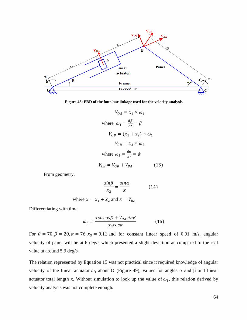
64
Figure 48: FBD of the four-bar linkage used for the velocity analysis
𝑉𝑂𝐴 = 𝑥1 × 𝜔1
where 𝜔1 = 𝑑𝛽𝑑𝑡
=
𝑉𝑂𝐵 = (𝑥1 + 𝑥2) × 𝜔1
𝑉𝐶𝐵 = 𝑥3 × 𝜔2
where 𝜔2 = 𝑑𝛼𝑑𝑡
=
𝑉𝐶𝐵 = 𝑉𝑂𝐵 + 𝑉𝐵𝐴 (13)
From geometry,
𝑠𝑖𝑛𝛽𝑥3
=𝑠𝑖𝑛𝛼𝑥
(14)
where 𝑥 = 𝑥1 + 𝑥2 and = 𝑉𝐵𝐴
Differentiating with time
𝜔2 =𝑥𝜔1𝑐𝑜𝑠𝛽 + 𝑉𝐵𝐴𝑠𝑖𝑛𝛽
𝑥3𝑐𝑜𝑠𝛼 (15)
For 𝜃 = 70,𝛽 = 20,𝛼 = 76, 𝑥3 = 0.11 and for constant linear speed of 0.01 m/s, angular
velocity of panel will be at 6 deg/s which presented a slight deviation as compared to the real
value at around 5.3 deg/s.
The relation represented by Equation 15 was not practical since it required knowledge of angular
velocity of the linear actuator 𝜔1 about O (Figure 49), values for angles α and β and linear
actuator total length x. Without simulation to look up the value of 𝜔1, this relation derived by
velocity analysis was not complete enough.
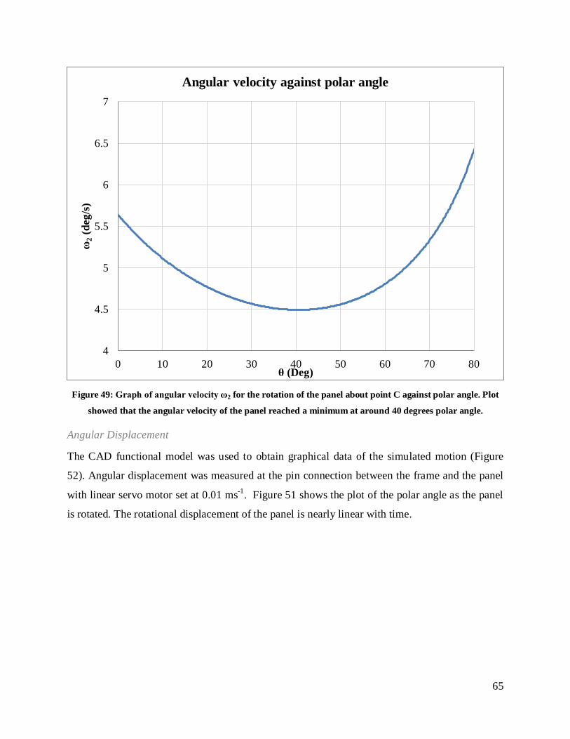
65
Figure 49: Graph of angular velocity ω2 for the rotation of the panel about point C against polar angle. Plot
showed that the angular velocity of the panel reached a minimum at around 40 degrees polar angle.
Angular Displacement
The CAD functional model was used to obtain graphical data of the simulated motion (Figure
52). Angular displacement was measured at the pin connection between the frame and the panel
with linear servo motor set at 0.01 ms-1. Figure 51 shows the plot of the polar angle as the panel
is rotated. The rotational displacement of the panel is nearly linear with time.
4
4.5
5
5.5
6
6.5
7
0 10 20 30 40 50 60 70 80
ω2 (
deg/
s)
θ (Deg)
Angular velocity against polar angle
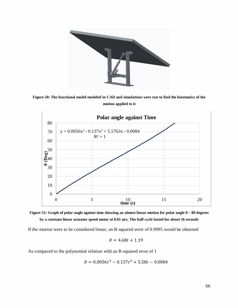
66
Figure 50: The functional model modeled in CAD and simulations were run to find the kinematics of the
motion applied to it
Figure 51: Graph of polar angle against time showing an almost linear motion for polar angle 0 – 80 degrees
by a constant linear actuator speed motor at 0.01 m/s. The half cycle lasted for about 16 seconds
If the motion were to be considered linear, an R-squared error of 0.9995 would be obtained
𝜃 = 4.68𝑡 + 1.19
As compared to the polynomial relation with an R-squared error of 1
𝜃 = 0.0056𝑡3 − 0.137𝑡2 + 5.58𝑡 − 0.0084
y = 0.0056x3 - 0.137x2 + 5.5763x - 0.0084 R² = 1
0
10
20
30
40
50
60
70
80
0 5 10 15 20
θ (D
eg)
time (s)
Polar angle against Time
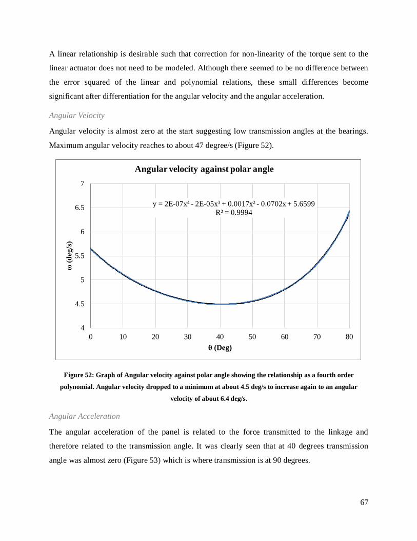
67
A linear relationship is desirable such that correction for non-linearity of the torque sent to the
linear actuator does not need to be modeled. Although there seemed to be no difference between
the error squared of the linear and polynomial relations, these small differences become
significant after differentiation for the angular velocity and the angular acceleration.
Angular Velocity
Angular velocity is almost zero at the start suggesting low transmission angles at the bearings.
Maximum angular velocity reaches to about 47 degree/s (Figure 52).
Figure 52: Graph of Angular velocity against polar angle showing the relationship as a fourth order
polynomial. Angular velocity dropped to a minimum at about 4.5 deg/s to increase again to an angular
velocity of about 6.4 deg/s.
Angular Acceleration
The angular acceleration of the panel is related to the force transmitted to the linkage and
therefore related to the transmission angle. It was clearly seen that at 40 degrees transmission
angle was almost zero (Figure 53) which is where transmission is at 90 degrees.
y = 2E-07x4 - 2E-05x3 + 0.0017x2 - 0.0702x + 5.6599 R² = 0.9994
4
4.5
5
5.5
6
6.5
7
0 10 20 30 40 50 60 70 80
ω (d
eg/s
)
θ (Deg)
Angular velocity against polar angle
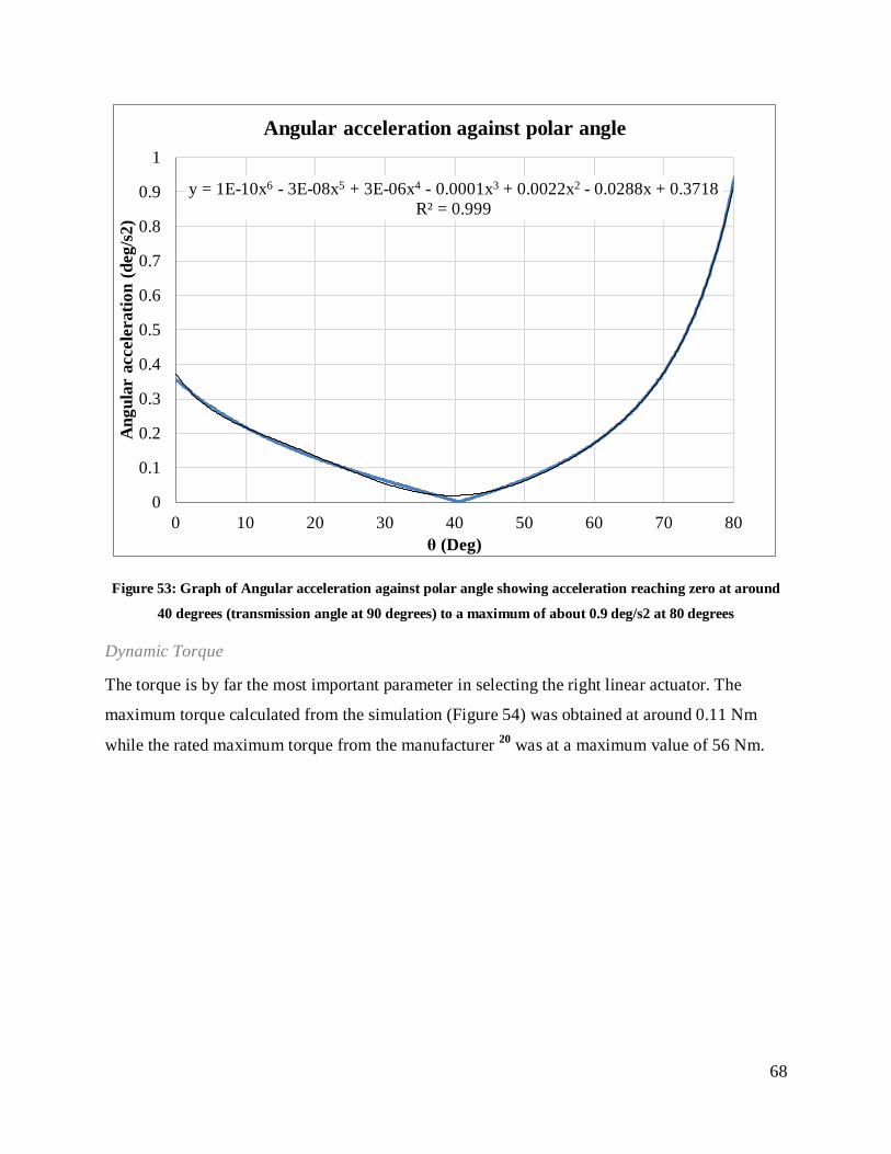
68
Figure 53: Graph of Angular acceleration against polar angle showing acceleration reaching zero at around
40 degrees (transmission angle at 90 degrees) to a maximum of about 0.9 deg/s2 at 80 degrees
Dynamic Torque
The torque is by far the most important parameter in selecting the right linear actuator. The
maximum torque calculated from the simulation (Figure 54) was obtained at around 0.11 Nm
while the rated maximum torque from the manufacturer 20 was at a maximum value of 56 Nm.
y = 1E-10x6 - 3E-08x5 + 3E-06x4 - 0.0001x3 + 0.0022x2 - 0.0288x + 0.3718 R² = 0.999
0
0.1
0.2
0.3
0.4
0.5
0.6
0.7
0.8
0.9
1
0 10 20 30 40 50 60 70 80
Ang
ular
acc
eler
atio
n (d
eg/s
2)
θ (Deg)
Angular acceleration against polar angle
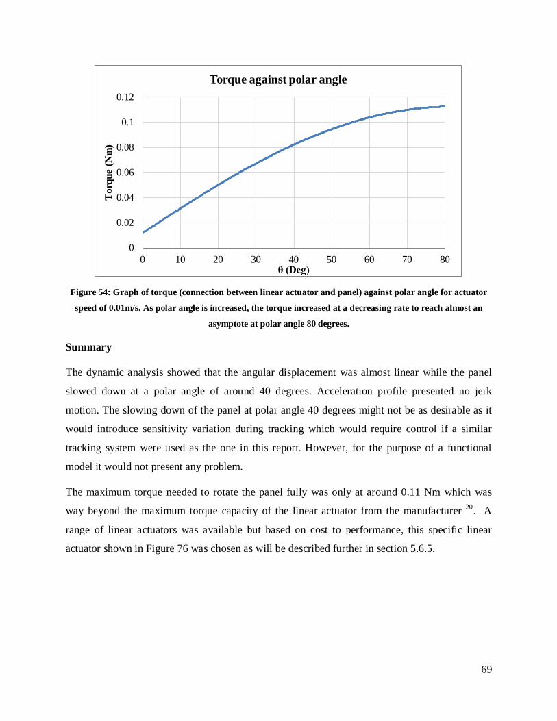
69
Figure 54: Graph of torque (connection between linear actuator and panel) against polar angle for actuator
speed of 0.01m/s. As polar angle is increased, the torque increased at a decreasing rate to reach almost an
asymptote at polar angle 80 degrees.
Summary
The dynamic analysis showed that the angular displacement was almost linear while the panel
slowed down at a polar angle of around 40 degrees. Acceleration profile presented no jerk
motion. The slowing down of the panel at polar angle 40 degrees might not be as desirable as it
would introduce sensitivity variation during tracking which would require control if a similar
tracking system were used as the one in this report. However, for the purpose of a functional
model it would not present any problem.
The maximum torque needed to rotate the panel fully was only at around 0.11 Nm which was
way beyond the maximum torque capacity of the linear actuator from the manufacturer 20. A
range of linear actuators was available but based on cost to performance, this specific linear
actuator shown in Figure 76 was chosen as will be described further in section 5.6.5.
0
0.02
0.04
0.06
0.08
0.1
0.12
0 10 20 30 40 50 60 70 80
Tor
que
(Nm
)
θ (Deg)
Torque against polar angle

70
5.5.2. Power Analysis
Power: Linear actuator
The power required to rotate the panel was essential in estimating the feasibility of the linear
actuator motor and the amount of power to send to it in order to follow the assigned kinematic
motion.
A number of assumptions were made for the kinematic motion which was used as validation for
the simulation. It was desirable that the azimuth rotation should be executed in less than 15
second (half cycle) and it was assumed that the model accelerated in 0.25 second only.
The definitions and values of the variables used were listed in Table 14 while mass moment of
inertia was calculated for the whole functional model in Appendix K. Power was found using
Equation 16. Power needed was found to be analytically 0.16 W however when simulated the
linear actuator was assigned a constant velocity which resulted in a varying angular velocity
from 4.5 rad/s to 6.4 rad/s. Simulated power increased to a maximum of about 0.7 W (Figure 55)
owing to the larger angular velocity and deceleration of 0.9 rad/s2.
Table 14: Definitions and values for the terms used in deriving the initial linear actuator power
Terms Definition Value
t Time for half cycle (s) 15
ωp Angular velocity of panel (rad/s) 0.093
αp Angular acceleration of panel (rad/s2) 0.37
Ip Mass moment of Inertia of panel (kgm2) 4.67
𝑷𝒍𝒂 Power required to rotate panel (W) 0.16
Power needed for linear actuator to rotate the panel initially was given by Equation 16
𝑃𝑙𝑎 ≥ 𝐼𝜔𝛼 (16)
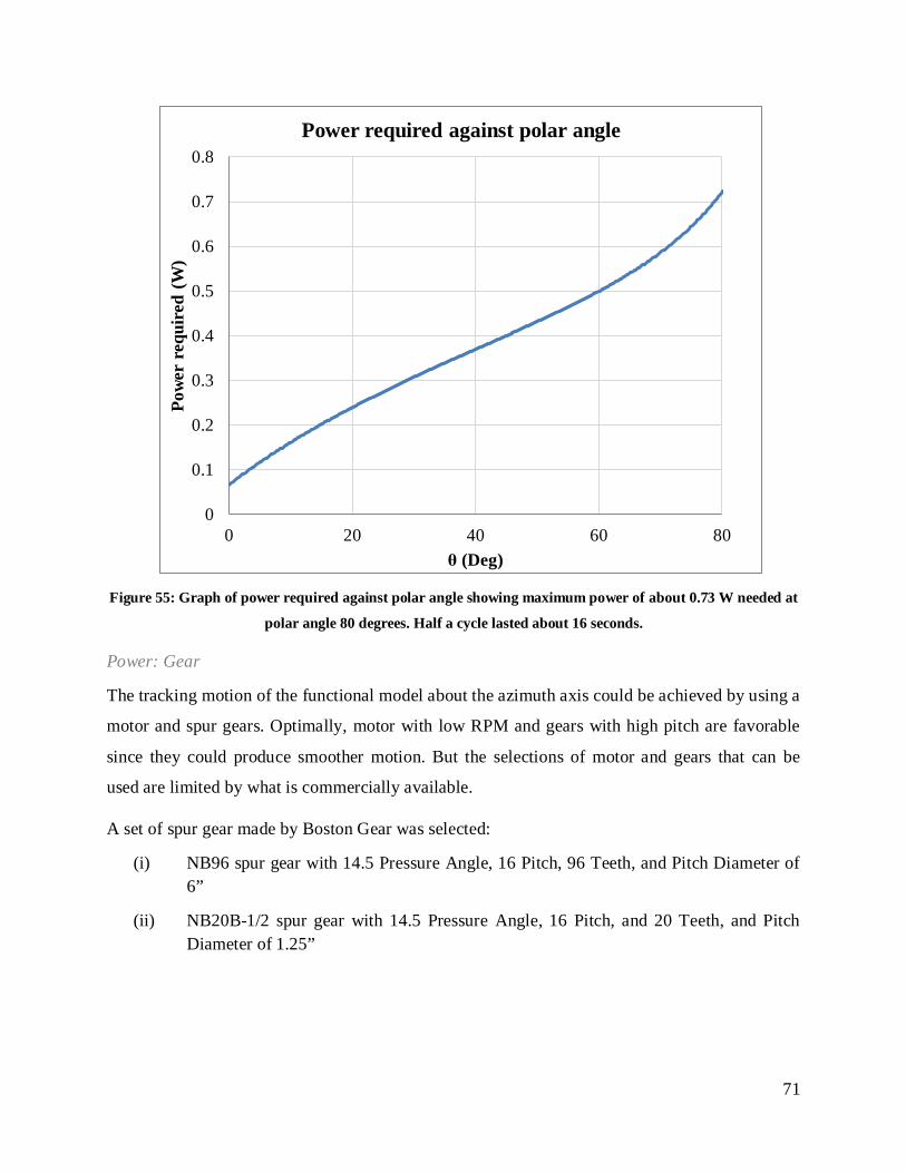
71
Figure 55: Graph of power required against polar angle showing maximum power of about 0.73 W needed at
polar angle 80 degrees. Half a cycle lasted about 16 seconds.
Power: Gear
The tracking motion of the functional model about the azimuth axis could be achieved by using a
motor and spur gears. Optimally, motor with low RPM and gears with high pitch are favorable
since they could produce smoother motion. But the selections of motor and gears that can be
used are limited by what is commercially available.
A set of spur gear made by Boston Gear was selected:
(i) NB96 spur gear with 14.5 Pressure Angle, 16 Pitch, 96 Teeth, and Pitch Diameter of 6”
(ii) NB20B-1/2 spur gear with 14.5 Pressure Angle, 16 Pitch, and 20 Teeth, and Pitch Diameter of 1.25”
0
0.1
0.2
0.3
0.4
0.5
0.6
0.7
0.8
0 20 40 60 80
Pow
er r
equi
red
(W)
θ (Deg)
Power required against polar angle

72
Given that polar rotation should be executed in less than thirty second and that model accelerated
in 1 second only, the power Pg required to turn the tracker could be calculated given by Equation
16. Torque was consequently calculated from the power as given by Equation 17. Values for
variables used in the calculation of power and torque was given in Table 15.
Torque needed to rotate the model:
𝜏 =𝑃𝜔
(17)
Table 15: Definitions and values of the variables used to derive gear power
Term Definition Value
tp Time to complete one cycle/s < 30
ωp Angular velocity of the gear/ rad/s 2π/30
αp Angular acceleration of the gear initially/ rad/s2 2π/30
𝑃𝑔 Power needed to rotate gear/W ≥ 0.219
𝜏 Torque required/ Nm 1.406
𝑃𝑚 Power of motor/ Nm 14
R Gear Ratio 4.8
The motor selected for the application (Figure 77) had a rated torque of 14N.m at 12V as
calculated by Equation 18. The motor would be connected to the smaller spur gear which rotates
around the bigger spur gear. The torque exerted on the model by the motor can be calculated by:
𝜏 = 𝑃𝑚 .𝑅 (18)
The torque output was found to be 67.2 Nm, which was a lot more than what the tracker needed,
so a pulse-width modulated signal would be used to power the motor in order to reduce the
torque.
5.5.3. State equation for the system motion
Determination of the Equation of motion of the system with both the linear actuator and the gear
driving the motion was derived using the Lagrangian Method. Virtual work equations for each
link in the functional model were derived in Appendix L:

73
The assumptions made for this analysis were:
1. All part bodies are rigid bodies so that only a change in CGs will alter the energy of the
system.
2. Gravitational forces of the members in moderate to high speed machinery often tend to be
dwarfed by the dynamic forces from the accelerating masses. In this project, the speed of
the functional model was assumed to be low so that gravitational force and gravitational
potential energy should be considered. However the CG of the panel is the only one that
changed with height and the change in distance was assumed small enough such that the
change in potential energy was neglected all along.
3. Pin jointed linages with low-friction bearings at the pivots can have high efficiencies of
95% and above which is why it is reasonable to assume that the pin joints are frictionless.
Therefore system was assumed a conservative system in an ideal environment.
The Equation of motion was given by Equation 19 and derived in Appendix L
𝑚𝑏21 + − 𝑚(𝑏2 + 𝑙2)𝑁2𝑠𝑖𝑛𝜑𝑐𝑜𝑠𝜑 = 0 (19)
However this was true only if panel was fixed at polar angle 0 degree and if no rotation was
imposed by the linear actuator as explained further in Appendix L which will reduce to the
simple basic equation of motion given as Equation 20.
𝑀 = 𝐼𝑥𝑥𝑥 (20)
5.6. Tracker Electronics
Figure 56 shows the overall electrical system of the functional model. The main power source of
the tracker was the 12V onboard battery, which could be charged using power from the solar
panel itself or from 110V AC socket. Both of them passed through a DC regulator and a charge
controller to avoid overcharging the battery. The user could choose which power source to use
via a switch on the tracker. The solar panel could be used during outdoor demonstration and the
AC socket could be used as power source for indoor demonstration of the model.
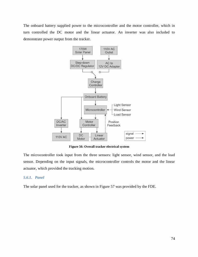
74
The onboard battery supplied power to the microcontroller and the motor controller, which in
turn controlled the DC motor and the linear actuator. An inverter was also included to
demonstrate power output from the tracker.
Figure 56: Overall tracker electrical system
The microcontroller took input from the three sensors: light sensor, wind sensor, and the load
sensor. Depending on the input signals, the microcontroller controls the motor and the linear
actuator, which provided the tracking motion.
5.6.1. Panel
The solar panel used for the tracker, as shown in Figure 57 was provided by the FDE.

75
Figure 57: SST 175-72M solar panel 22
Information about the panel is listed in Table 15.
Table 16: Information about the SST 175-72M panel 22
Manufacturer CEEG Shanghai Solar Science and Technology
Model SST 175-72M
Cell Type Monocrystalline Cell
Cell Size 125 mm x 125 mm
(4.92 in x 4.92 in)
Cells 6 x 12
Dimensions 1580 mm x 808 mm x 50 mm
(62.2 in x 31.8 in x 1.9 in)
Weight 16 kg
(35.5 lbs)
STC Power Rating 175 W
PTC Power Rating 156.5 W
Open Circuit Voltage 44.5 V
Short Circuit Current 5.34 A
Voltage at Maximum Power 35.3 V
Current at Maximum Power 4.96 A
Panel Efficiency 13.7%
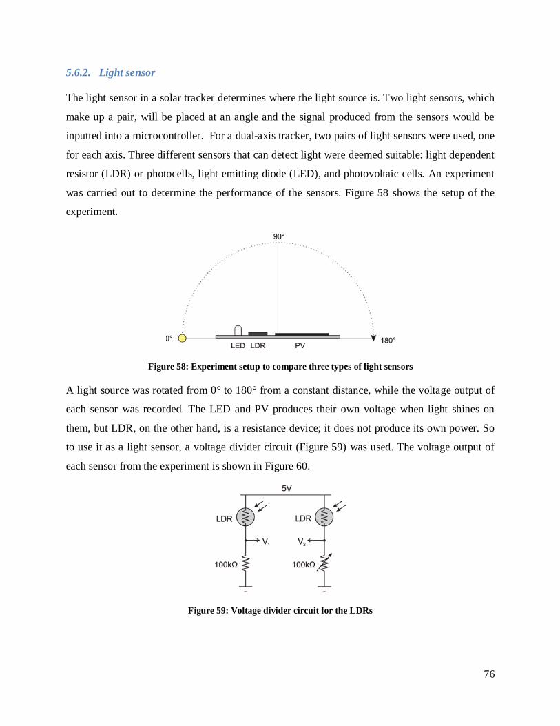
76
5.6.2. Light sensor
The light sensor in a solar tracker determines where the light source is. Two light sensors, which
make up a pair, will be placed at an angle and the signal produced from the sensors would be
inputted into a microcontroller. For a dual-axis tracker, two pairs of light sensors were used, one
for each axis. Three different sensors that can detect light were deemed suitable: light dependent
resistor (LDR) or photocells, light emitting diode (LED), and photovoltaic cells. An experiment
was carried out to determine the performance of the sensors. Figure 58 shows the setup of the
experiment.
Figure 58: Experiment setup to compare three types of light sensors
A light source was rotated from 0° to 180° from a constant distance, while the voltage output of
each sensor was recorded. The LED and PV produces their own voltage when light shines on
them, but LDR, on the other hand, is a resistance device; it does not produce its own power. So
to use it as a light sensor, a voltage divider circuit (Figure 59) was used. The voltage output of
each sensor from the experiment is shown in Figure 60.
Figure 59: Voltage divider circuit for the LDRs
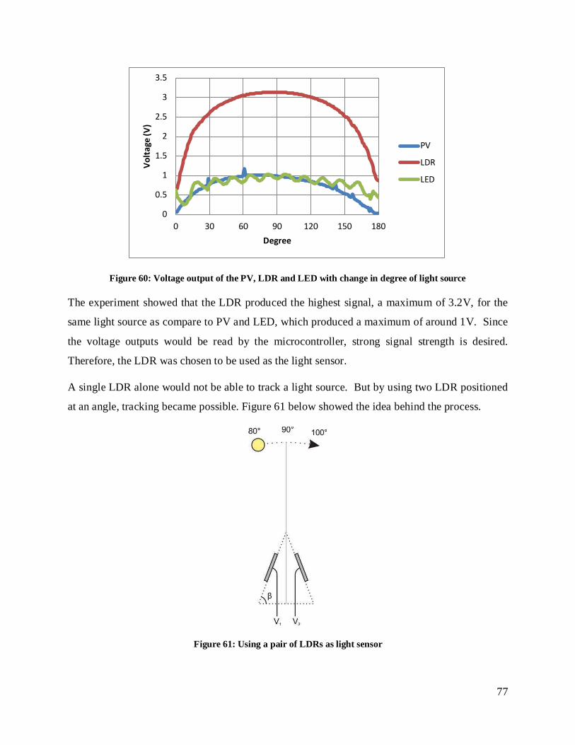
77
Figure 60: Voltage output of the PV, LDR and LED with change in degree of light source
The experiment showed that the LDR produced the highest signal, a maximum of 3.2V, for the
same light source as compare to PV and LED, which produced a maximum of around 1V. Since
the voltage outputs would be read by the microcontroller, strong signal strength is desired.
Therefore, the LDR was chosen to be used as the light sensor.
A single LDR alone would not be able to track a light source. But by using two LDR positioned
at an angle, tracking became possible. Figure 61 below showed the idea behind the process.
Figure 61: Using a pair of LDRs as light sensor
0
0.5
1
1.5
2
2.5
3
3.5
0 30 60 90 120 150 180
Volta
ge (V
)
Degree
PV
LDR
LED
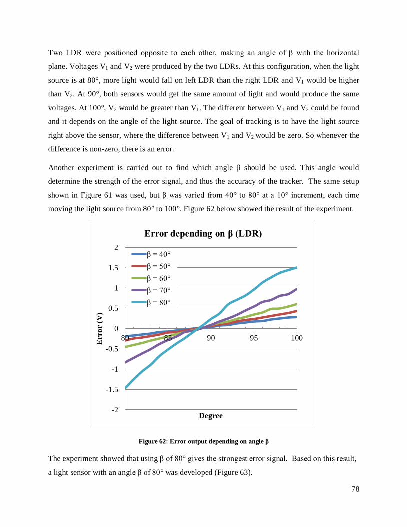
78
Two LDR were positioned opposite to each other, making an angle of β with the horizontal
plane. Voltages V1 and V2 were produced by the two LDRs. At this configuration, when the light
source is at 80°, more light would fall on left LDR than the right LDR and V1 would be higher
than V2. At 90°, both sensors would get the same amount of light and would produce the same
voltages. At 100°, V2 would be greater than V1. The different between V1 and V2 could be found
and it depends on the angle of the light source. The goal of tracking is to have the light source
right above the sensor, where the difference between V1 and V2 would be zero. So whenever the
difference is non-zero, there is an error.
Another experiment is carried out to find which angle β should be used. This angle would
determine the strength of the error signal, and thus the accuracy of the tracker. The same setup
shown in Figure 61 was used, but β was varied from 40° to 80° at a 10° increment, each time
moving the light source from 80° to 100°. Figure 62 below showed the result of the experiment.
Figure 62: Error output depending on angle β
The experiment showed that using β of 80° gives the strongest error signal. Based on this result,
a light sensor with an angle β of 80° was developed (Figure 63).
-2
-1.5
-1
-0.5
0
0.5
1
1.5
2
80 85 90 95 100Err
or (V
)
Degree
Error depending on β (LDR)
β = 40° β = 50° β = 60° β = 70° β = 80°
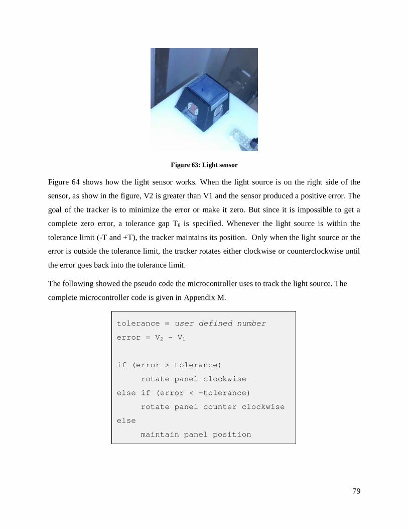
79
Figure 63: Light sensor
Figure 64 shows how the light sensor works. When the light source is on the right side of the
sensor, as show in the figure, V2 is greater than V1 and the sensor produced a positive error. The
goal of the tracker is to minimize the error or make it zero. But since it is impossible to get a
complete zero error, a tolerance gap Tθ is specified. Whenever the light source is within the
tolerance limit (-T and +T), the tracker maintains its position. Only when the light source or the
error is outside the tolerance limit, the tracker rotates either clockwise or counterclockwise until
the error goes back into the tolerance limit.
The following showed the pseudo code the microcontroller uses to track the light source. The
complete microcontroller code is given in Appendix M.
tolerance = user defined number
error = V2 – V1
if (error > tolerance)
rotate panel clockwise
else if (error < -tolerance)
rotate panel counter clockwise
else
maintain panel position
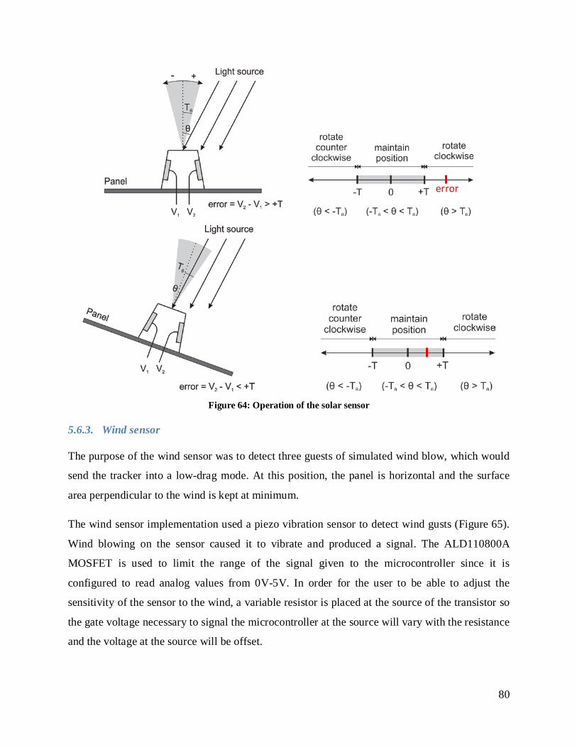
80
Figure 64: Operation of the solar sensor
5.6.3. Wind sensor
The purpose of the wind sensor was to detect three guests of simulated wind blow, which would
send the tracker into a low-drag mode. At this position, the panel is horizontal and the surface
area perpendicular to the wind is kept at minimum.
The wind sensor implementation used a piezo vibration sensor to detect wind gusts (Figure 65).
Wind blowing on the sensor caused it to vibrate and produced a signal. The ALD110800A
MOSFET is used to limit the range of the signal given to the microcontroller since it is
configured to read analog values from 0V-5V. In order for the user to be able to adjust the
sensitivity of the sensor to the wind, a variable resistor is placed at the source of the transistor so
the gate voltage necessary to signal the microcontroller at the source will vary with the resistance
and the voltage at the source will be offset.
error
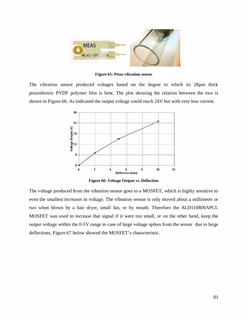
81
Figure 65: Piezo vibration sensor
The vibration sensor produced voltages based on the degree to which its 28µm thick
piezoelectric PVDF polymer film is bent. The plot showing the relation between the two is
shown in Figure 66. As indicated the output voltage could reach 24V but with very low current.
Figure 66: Voltage Output vs. Deflection
The voltage produced from the vibration sensor goes to a MOSFET, which is highly sensitive to
even the smallest increases in voltage. The vibration sensor is only moved about a millimeter or
two when blown by a hair dryer, small fan, or by mouth. Therefore the ALD110800APCL
MOSFET was used to increase that signal if it were too small, or on the other hand, keep the
output voltage within the 0-5V range in case of large voltage spikes from the sensor due to large
deflections. Figure 67 below showed the MOSFET’s characteristic.
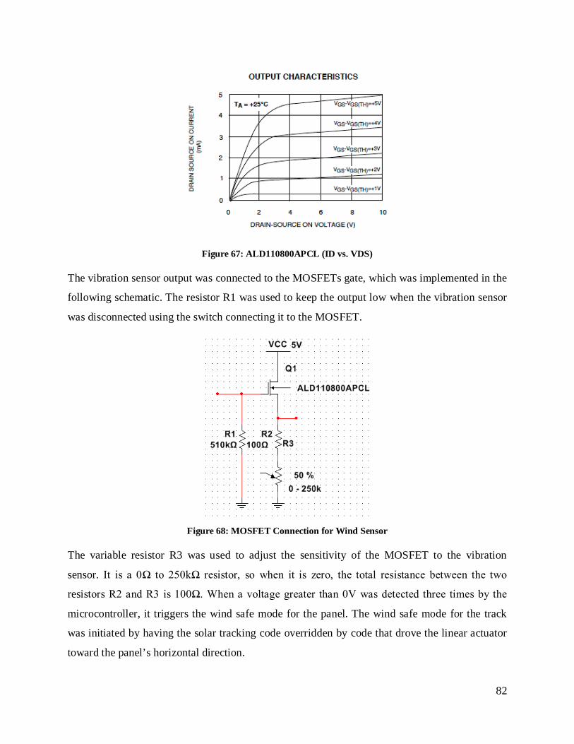
82
Figure 67: ALD110800APCL (ID vs. VDS)
The vibration sensor output was connected to the MOSFETs gate, which was implemented in the
following schematic. The resistor R1 was used to keep the output low when the vibration sensor
was disconnected using the switch connecting it to the MOSFET.
Figure 68: MOSFET Connection for Wind Sensor
The variable resistor R3 was used to adjust the sensitivity of the MOSFET to the vibration
sensor. It is a 0Ω to 250kΩ resistor, so when it is zero, the total resistance between the two
resistors R2 and R3 is 100Ω. When a voltage greater than 0V was detected three times by the
microcontroller, it triggers the wind safe mode for the panel. The wind safe mode for the track
was initiated by having the solar tracking code overridden by code that drove the linear actuator
toward the panel’s horizontal direction.

83
During initial testing, the wind sensor worked but the variable resistor had to be turned all the
way down to make the wind sensor sensitive to wind blow from the mouth. The piezo sensor was
made of a hard plastic material and it was hard to bend it using wind force. Another problem
came up when the sensor was tested on the panel. During tracking, the tracker vibrates and the
wind sensor, made of a vibration sensor, picked up the movement causing false readings.
After unsuccessful tryouts, the wind sensor was replaced with a thermal anemometer (Figure 69).
The device works by heating a resistor to a constant temperature and the electrical power
required to maintain temperature is measured. As the wind blew over the resistor, the
temperature dropped and the resistor drew more power to keep the temperature constant.
Figure 69: Thermal anemometer
The anemometer already includes an onboard circuit which takes in 5V and outputs a voltage
ranging from 0-5V depending on the wind speed. The output voltage could the inputted directly
into the microcontroller. The anemometer was rated to sense wind speeds from 0 to 30mph.
5.6.4. Load sensor
The functional model also required a load sensor to detect the simulated snow weight that may
accumulate on the solar panel. The load sensor was designed to measure the amount of weight
placed on the sensor. The purpose is to tilt the solar panel to 80° when the weight measured by
the sensor reached a certain threshold. The panel would be held at the 80° position until the
weight slide off the panel.
The main challenge presented was determining how to design a load sensor. From research, it
was found that the resistive property of a type of conductive foam could be used to implement a
load sensor. The conductive foam used to package integrated circuits has an inverse relationship
between compression and resistance. A piece of the foam has an initial resistance with no weight
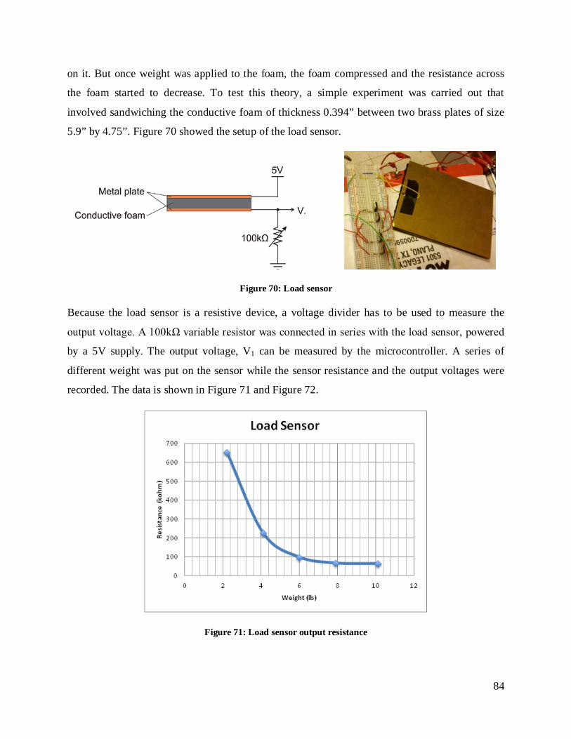
84
on it. But once weight was applied to the foam, the foam compressed and the resistance across
the foam started to decrease. To test this theory, a simple experiment was carried out that
involved sandwiching the conductive foam of thickness 0.394” between two brass plates of size
5.9” by 4.75”. Figure 70 showed the setup of the load sensor.
Figure 70: Load sensor
Because the load sensor is a resistive device, a voltage divider has to be used to measure the
output voltage. A 100kΩ variable resistor was connected in series with the load sensor, powered
by a 5V supply. The output voltage, V1 can be measured by the microcontroller. A series of
different weight was put on the sensor while the sensor resistance and the output voltages were
recorded. The data is shown in Figure 71 and Figure 72.
Figure 71: Load sensor output resistance
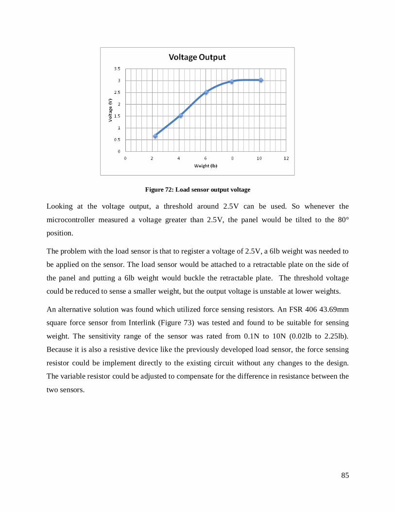
85
Figure 72: Load sensor output voltage
Looking at the voltage output, a threshold around 2.5V can be used. So whenever the
microcontroller measured a voltage greater than 2.5V, the panel would be tilted to the 80°
position.
The problem with the load sensor is that to register a voltage of 2.5V, a 6lb weight was needed to
be applied on the sensor. The load sensor would be attached to a retractable plate on the side of
the panel and putting a 6lb weight would buckle the retractable plate. The threshold voltage
could be reduced to sense a smaller weight, but the output voltage is unstable at lower weights.
An alternative solution was found which utilized force sensing resistors. An FSR 406 43.69mm
square force sensor from Interlink (Figure 73) was tested and found to be suitable for sensing
weight. The sensitivity range of the sensor was rated from 0.1N to 10N (0.02lb to 2.25lb).
Because it is also a resistive device like the previously developed load sensor, the force sensing
resistor could be implement directly to the existing circuit without any changes to the design.
The variable resistor could be adjusted to compensate for the difference in resistance between the
two sensors.

86
Figure 73: FSR 406 Force resistive sensor
5.6.5. Linear Actuator
A 12V 6” stroke linear actuator, shown in Figure 74, is used to provide motion to the panel about
the polar or horizontal axis.
Figure 74: ServoCity 6-12V DC 6” stroke linear actuator 20
Information about the linear actuator is shown below in Table 16.
Table 17: Information about the ServoCity linear actuator
Manufacturer ServoCity Operating Voltage 6.0 ~ 12.0 V DC Operating Temperature -20 ~ +65 °C
-14.8 ~ +149 °F Operating Speed @ 12 V .50”/second (No load)
.39”/second (Maximum load) Dynamic Thrust 115 lbs Static Load 500 lbs Current Rating @ 12 V 700mA (No load) Motor Type 3 Pole Ferrite Potentiometer 10kΩ Gear Ratio 20:1 Duty Cycle 25%

87
5.6.6. DC Motor
The 12V DC motor (Figure 75) is used to provide rotational motion about the vertical or azimuth axis.
Figure 75: AM Equipment 214 Series Gearhead Motor 23
Information about the motor is shown below in Table 17
Table 18: Information about the AM Equipment 214 Series Gearhead Motor 23
Manufacturer AM Equipment
Voltage 12.0 V DC
Torque 14 Nm
Weight 1.6 lb
No load
Speed (rpm)
Current (A)
75.9 ~ 62.1
3.3 ~ 2.7
Stall load
Speed (rpm)
Current (A)
19.4 ~ 15.9
31.7 ~ 26
Peak power
Speed (rpm)
Current (A)
36.5 ~ 30
10.5 ~ 8.6

88
5.7. Design and Manufacturing
Most of the design features from the STS444 were included in the functional model; it contained
the base with the slewing gears and motor, two vertical beams (or) dual towers, two vertical
cross beams to support the panel, and a linear actuator in place of the screw jack. Figure 76
below showed the overview of the functional model. The blueprints of the major parts are
shown in Appendix N.
Figure 76: Overview design of the functional model
5.7.1. Panel Assembly
The panel assembly is shown in Figure 77 below. To connect the solar panel to the tracker frame,
two vertical cross beams made from 3/8” thick aluminum bars were used. They were bolted to
four aluminum brackets (made from 1” x 2” aluminum tubing), which were then bolted to the
panel’s side frame. Another aluminum beam, made out of 1” x 1” square tubing was also
attached across the center of the panel. It would be attached to the linear actuator, which rotates
the panel around the horizontal axis.

89
Figure 77: Two vertical cross beams and the center beam connected to the panel
Figure 80 showed how the two vertical cross beams were connected to the towers using a
shoulder bolt and two flanged bearings on each side, so that the cross beams could rotate about
the horizontal axis (See Figure 79 for the cross section view of the connection). The towers were
made of 1” x 2” rectangular tubing. Another horizontal beam was attached to the side of the
tower beams. A bracket was connected to it, which supports the lower end of linear actuator used
to rotate the panel. The top end of the linear actuator was connected to the center square tubing
using a ball-lock pin for easy removal.
Figure 78: Two tower beams connected to the cross beams

90
Figure 79: Cross section view of the connection
The assembly shown in Figure 78 made up the upper half of the tracker, the panel module. The
panel module could be attached to the lower half of the tracker, called the base module. The base
module provides stability to the tracker, contains a DC motor and gears to provide a rotation
along the vertical axis, and contains an electronic box to house the control systems and a battery.
5.7.2. Base Assembly
The assembly of the base module, which is 40” long and 32” wide, started with the legs (Figure
80), welded together using 1” x 2” aluminum tubes.
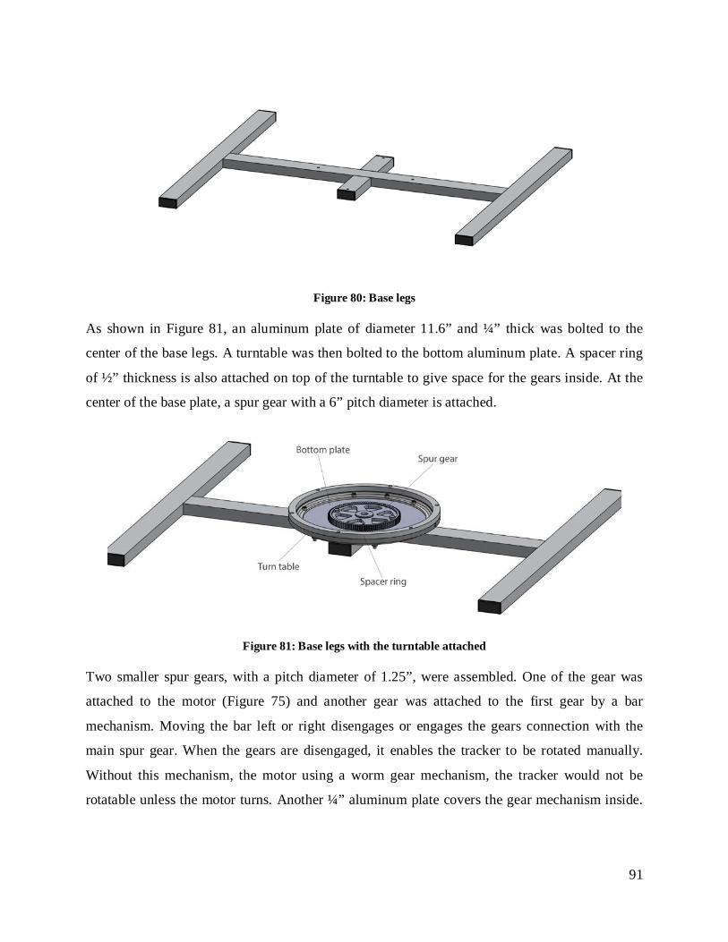
91
Figure 80: Base legs
As shown in Figure 81, an aluminum plate of diameter 11.6” and ¼” thick was bolted to the
center of the base legs. A turntable was then bolted to the bottom aluminum plate. A spacer ring
of ½” thickness is also attached on top of the turntable to give space for the gears inside. At the
center of the base plate, a spur gear with a 6” pitch diameter is attached.
Figure 81: Base legs with the turntable attached
Two smaller spur gears, with a pitch diameter of 1.25”, were assembled. One of the gear was
attached to the motor (Figure 75) and another gear was attached to the first gear by a bar
mechanism. Moving the bar left or right disengages or engages the gears connection with the
main spur gear. When the gears are disengaged, it enables the tracker to be rotated manually.
Without this mechanism, the motor using a worm gear mechanism, the tracker would not be
rotatable unless the motor turns. Another ¼” aluminum plate covers the gear mechanism inside.
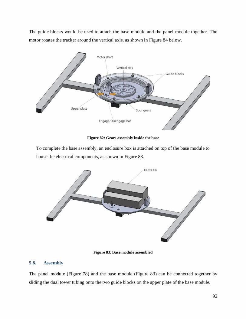
92
The guide blocks would be used to attach the base module and the panel module together. The
motor rotates the tracker around the vertical axis, as shown in Figure 84 below.
Figure 82: Gears assembly inside the base
To complete the base assembly, an enclosure box is attached on top of the base module to
house the electrical components, as shown in Figure 83.
Figure 83: Base module assembled
5.8. Assembly
The panel module (Figure 78) and the base module (Figure 83) can be connected together by
sliding the dual tower tubing onto the two guide blocks on the upper plate of the base module.

93
Figure 84: Attaching the panel and base module
The two ball lock pins could then be inserted into the hole through the dual towers and the guide
blocks to lock the two assemblies. Finally, the cable from the solar panel, sensors, and the linear
actuator were attached to their specific ports on the electric box. The power cable can be
connected to the wall socket to power the tracker and to charge the battery.
The panel module and the base module could also be connected to form a configuration for easy
transportation, as show in Figure 85 below. By utilizing the casters and the handles, the tracker
can either be pulled like a luggage or be pushed like a cart (Figure 86). Figure 89 showed the
procedure on how to assemble the tracker from the transportation mode.
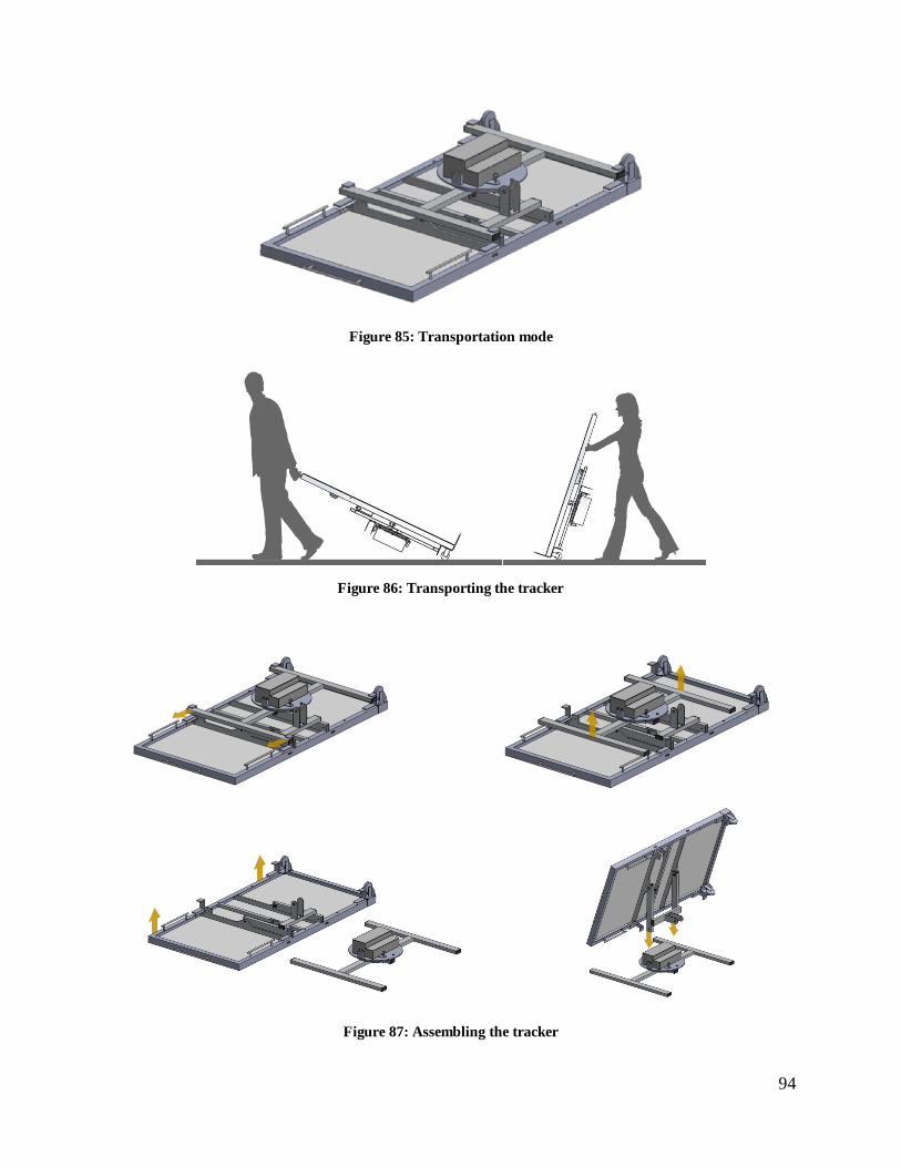
94
Figure 85: Transportation mode
Figure 86: Transporting the tracker
Figure 87: Assembling the tracker

95
5.9. Final design
The figures below show the actual photograph of the assembled functional model.
Figure 88: Functional model features
Figure 89: Functional model at low-drag position
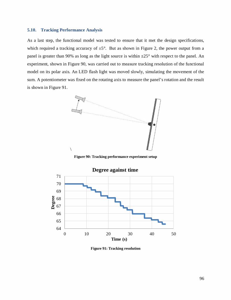
96
5.10. Tracking Performance Analysis
As a last step, the functional model was tested to ensure that it met the design specifications,
which required a tracking accuracy of ±5°. But as shown in Figure 2, the power output from a
panel is greater than 90% as long as the light source is within ±25° with respect to the panel. An
experiment, shown in Figure 90, was carried out to measure tracking resolution of the functional
model on its polar axis. An LED flash light was moved slowly, simulating the movement of the
sum. A potentiometer was fixed on the rotating axis to measure the panel’s rotation and the result
is shown in Figure 91.
\ Figure 90: Tracking performance experiment setup
Figure 91: Tracking resolution
64
65
66
67
68
69
70
71
0 10 20 30 40 50
Deg
ree
Time (s)
Degree against time

97
The data showed that the tracker could rotate at an increment of around 0.3° in the polar axis,
which is the resolution of the tracker. The result was a lot better than the required resolution of
±5°.
5.11. Conclusion
The functional model manufactured met all the design specifications and exceeds the
specification in some cases. The functional model was designed to have two parts, exceeding the
design requirement. It could be assembled and disassembled by two people and could be
transported by a single person with the help of the casters and handles attached to the panel. The
model, in its transportation mode, also met the design envelope stated. It could be assembled
from the transportation mode to a tracking mode in 4 simple steps. The weight of the final
functional model was around 70lb. The three required sensor were successfully integrated into
the function model. Finally, the tracking performance showed that the tracking resolution for the
polar axis was 0.3°, exceeding the required resolution of ±5°.

98
APPENDIX A
The design model of the STS 444 was modeled based on the blueprints provided by the FDE.
Most dimensions (Figure 92 - Figure 94) that were given were kept to ensure accuracy while
those that were not given were estimated to the best of our abilities. Stabilizing pods and some
extra reinforcing beams were omitted to simplify both the simulations and reduced scaled
prototype fabrication. Since deformation analysis were not carried out on the beams with lack of
material knowledge and proper dimensions, omitting beams would not affect the overall wind
load analysis.
Figure 92: Top view of STS444 with dimensions in meters.
Figure 93: Side view of STS444 with dimensions in meters.
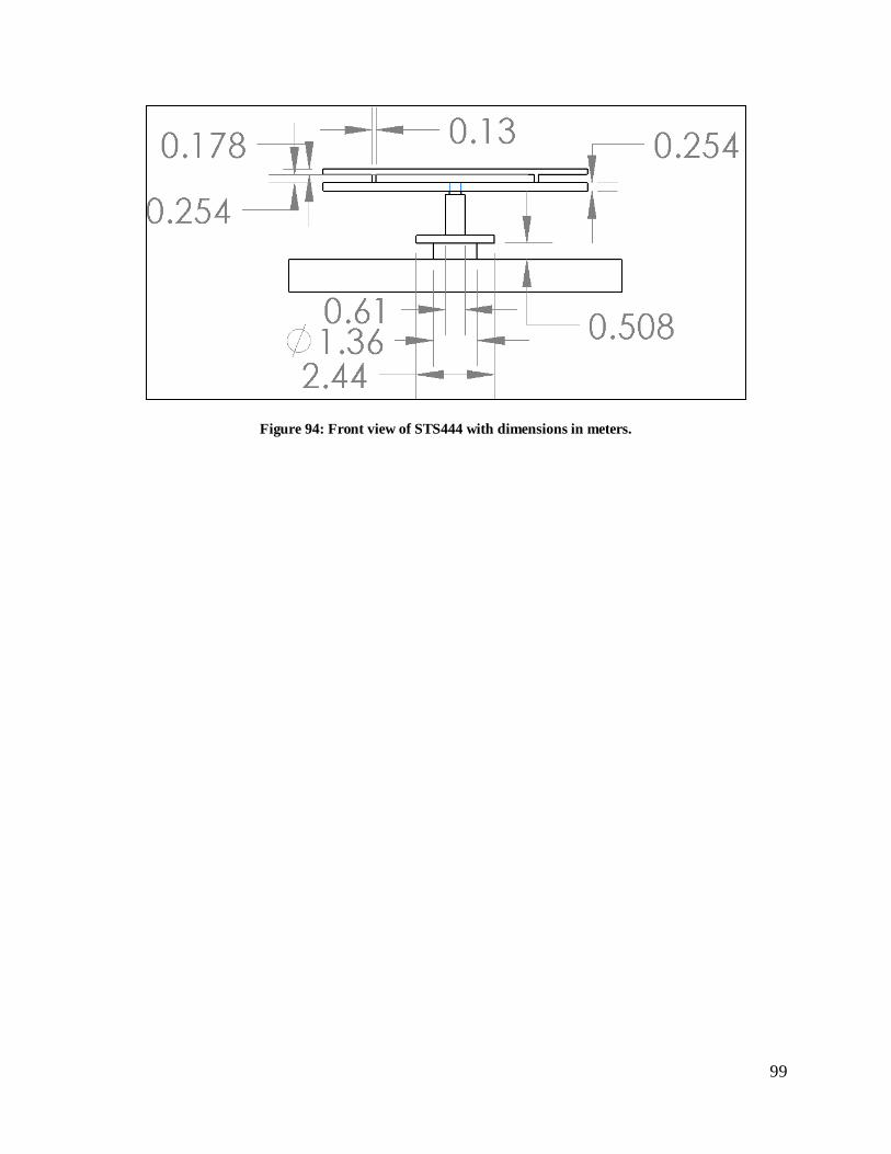
99
Figure 94: Front view of STS444 with dimensions in meters.
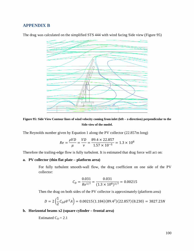
100
APPENDIX B
The drag was calculated on the simplified STS 444 with wind facing Side view (Figure 95)
Figure 95: Side View Contour lines of wind velocity coming from inlet (left – z-direction) perpendicular to the
Side view of the model.
The Reynolds number given by Equation 1 along the PV collector (22.857m long)
𝑅𝑒 =𝜌𝑉𝐷𝜇
=𝑉𝐷𝜈
=89.4 × 22.857
1.57 × 10−5= 1.3 × 10⁸
Therefore the trailing-edge flow is fully turbulent. It is estimated that drag force will act on:
a. PV collector (thin flat plate – platform area)
For fully turbulent smooth-wall flow, the drag coefficient on one side of the PV collector:
𝐶𝐷 =0.031𝑅𝑒1/7 =
0.031(1.3 × 10⁸)1/7 = 0.00215
Then the drag on both sides of the PV collector is approximately (platform area)
𝐷 = 2 12𝐶𝐷𝜌𝑉2𝐴 = 0.00215(1.184)(89.42)(22.857)(8.230) = 3827.23𝑁
b. Horizontal beams x2 (square cylinder – frontal area)
Estimated CD = 2.1

101
𝐷 = 2 12𝐶𝐷𝜌𝑉2𝐴 = (2.1)(1.184)(89.42)(0.254)(0.13) = 656.20𝑁
c. Frame support x2 (flat nose section – frontal area)
L/H ratio = 1.270/0.610 = 2.1
Estimated CD ~ 1.8
𝐷 = 2 12𝐶𝐷𝜌𝑉2𝐴 = 1.8(1.184)(89.42)(1.270)(0.610) = 13195.71𝑁
d. Rectangular turn-table (thin flat plate – platform area)
Reynolds Number 𝑅𝑒 = 89.4×2.441.57×10−5
= 1.4 × 10⁷ (Fully turbulent)
Estimated 𝐶𝐷 = 0.031𝑅𝑒1/7 = 0.031
(1.4×10⁷)1/7 = 0.00296
𝐷 = 2 12𝐶𝐷𝜌𝑉2𝐴 = 0.00296(1.184)(89.42)(2.440)(7.315) = 500𝑁
e. Gear (circular cylinder – frontal area)
Estimated CD ~ 2.2 (worst case)
𝐷 = 12𝐶𝐷𝜌𝑉2𝐴 = 0.5(2.2)(1.184)(89.42)
𝜋 × 1.362
4 = 15121.23𝑁
f. Base (flat nose section – frontal area)
L/H ratio = 1.016/13.360=0.076
Estimated CD ~ 1.2
𝐷 = 12𝐶𝐷𝜌𝑉2𝐴 = 0.5(1.2)(1.184)(89.42)(1.016)(13.360) = 77068.72𝑁
Total drag in X-direction = 1.11E5N
Determining CD of panel at different angle based on projected frontal area only. All other
components have a fixed CD since the frontal area is not changing. However drag on other
components will depend on how much of the component surface area is blocked by the panel.
For example when tilt angle is at 0 degrees, the only wetted area will be the PV panel and the
base or when the tilt angle is at 30 degrees the wetted areas include those of the panel, base,
cylinder, turn-table and half of the frame support towers surface area listed in Table 18.
At angle = 10 degrees
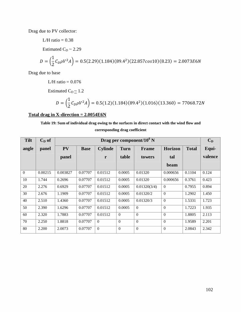
102
Drag due to PV collector:
L/H ratio = 0.38
Estimated CD ~ 2.29
𝐷 = 12𝐶𝐷𝜌𝑉2𝐴 = 0.5(2.29)(1.184)(89.42)(22.857𝑐𝑜𝑠10)(8.23) = 2.0073𝐸6𝑁
Drag due to base
L/H ratio = 0.076
Estimated CD ~ 1.2
𝐷 = 12𝐶𝐷𝜌𝑉2𝐴 = 0.5(1.2)(1.184)(89.42)(1.016)(13.360) = 77068.72𝑁
Total drag in X-direction = 2.0054E6N
Table 19: Sum of individual drag owing to the surfaces in direct contact with the wind flow and
corresponding drag coefficient
Tilt
angle
CD of
panel
Drag per component/106 N CD
Equi-
valence
PV
panel
Base Cylinde
r
Turn
table
Frame
towers
Horizon
tal
beam
Total
0 0.00215 0.003827 0.07707 0.01512 0.0005 0.01320 0.000656 0.1104 0.124
10 1.744 0.2696 0.07707 0.01512 0.0005 0.01320 0.000656 0.3761 0.423
20 2.276 0.6929 0.07707 0.01512 0.0005 0.01320(3/4) 0 0.7955 0.894
30 2.676 1.1909 0.07707 0.01512 0.0005 0.01320/2 0 1.2902 1.450
40 2.510 1.4360 0.07707 0.01512 0.0005 0.01320/3 0 1.5331 1.723
50 2.390 1.6296 0.07707 0.01512 0.0005 0 0 1.7223 1.935
60 2.320 1.7883 0.07707 0.01512 0 0 0 1.8805 2.113
70 2.250 1.8818 0.07707 0 0 0 0 1.9589 2.201
80 2.200 2.0073 0.07707 0 0 0 0 2.0843 2.342
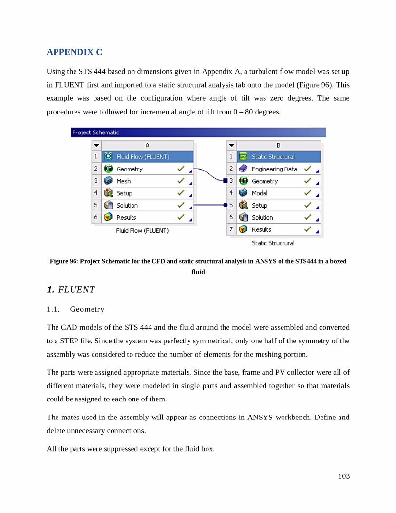
103
APPENDIX C
Using the STS 444 based on dimensions given in Appendix A, a turbulent flow model was set up
in FLUENT first and imported to a static structural analysis tab onto the model (Figure 96). This
example was based on the configuration where angle of tilt was zero degrees. The same
procedures were followed for incremental angle of tilt from 0 – 80 degrees.
Figure 96: Project Schematic for the CFD and static structural analysis in ANSYS of the STS444 in a boxed
fluid
1. FLUENT
1.1. Geometry
The CAD models of the STS 444 and the fluid around the model were assembled and converted
to a STEP file. Since the system was perfectly symmetrical, only one half of the symmetry of the
assembly was considered to reduce the number of elements for the meshing portion.
The parts were assigned appropriate materials. Since the base, frame and PV collector were all of
different materials, they were modeled in single parts and assembled together so that materials
could be assigned to each one of them.
The mates used in the assembly will appear as connections in ANSYS workbench. Define and
delete unnecessary connections.
All the parts were suppressed except for the fluid box.
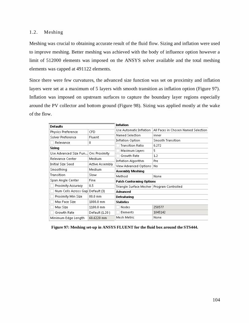
104
1.2. Meshing
Meshing was crucial to obtaining accurate result of the fluid flow. Sizing and inflation were used
to improve meshing. Better meshing was achieved with the body of influence option however a
limit of 512000 elements was imposed on the ANSYS solver available and the total meshing
elements was capped at 491122 elements.
Since there were few curvatures, the advanced size function was set on proximity and inflation
layers were set at a maximum of 5 layers with smooth transition as inflation option (Figure 97).
Inflation was imposed on upstream surfaces to capture the boundary layer regions especially
around the PV collector and bottom ground (Figure 98). Sizing was applied mostly at the wake
of the flow.
Figure 97: Meshing set-up in ANSYS FLUENT for the fluid box around the STS444.
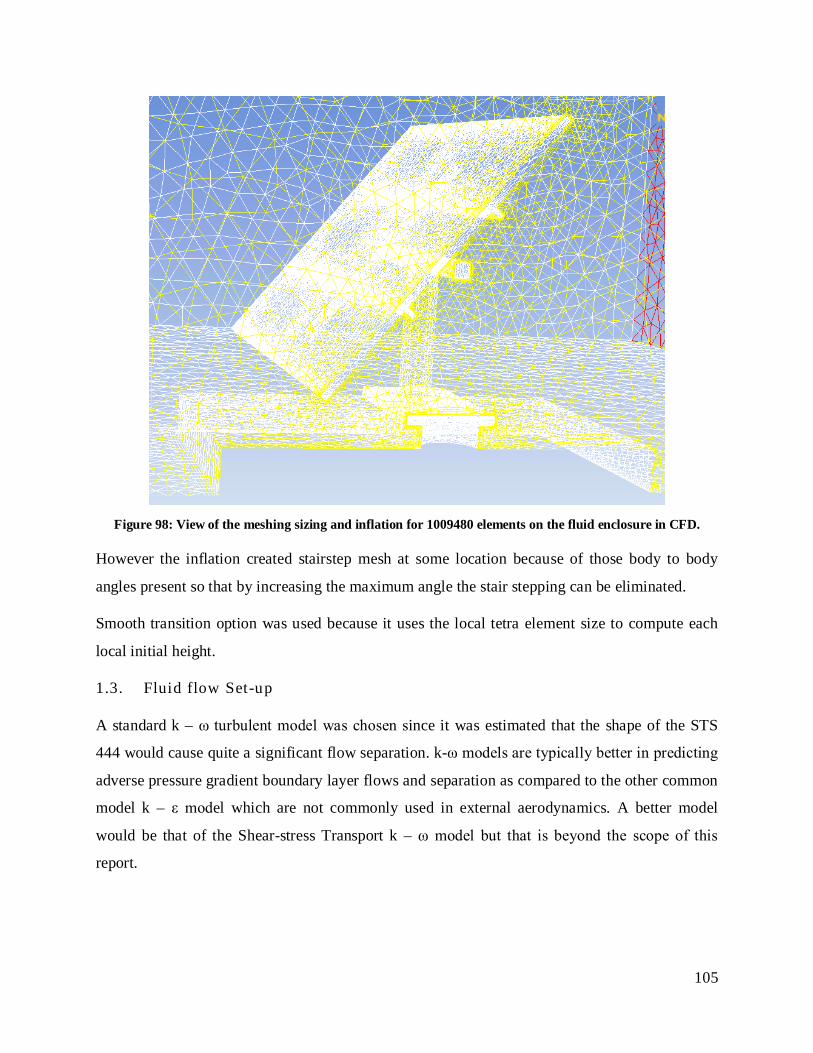
105
Figure 98: View of the meshing sizing and inflation for 1009480 elements on the fluid enclosure in CFD.
However the inflation created stairstep mesh at some location because of those body to body
angles present so that by increasing the maximum angle the stair stepping can be eliminated.
Smooth transition option was used because it uses the local tetra element size to compute each
local initial height.
1.3. Fluid flow Set-up
A standard k – ω turbulent model was chosen since it was estimated that the shape of the STS
444 would cause quite a significant flow separation. k-ω models are typically better in predicting
adverse pressure gradient boundary layer flows and separation as compared to the other common
model k – ε model which are not commonly used in external aerodynamics. A better model
would be that of the Shear-stress Transport k – ω model but that is beyond the scope of this
report.
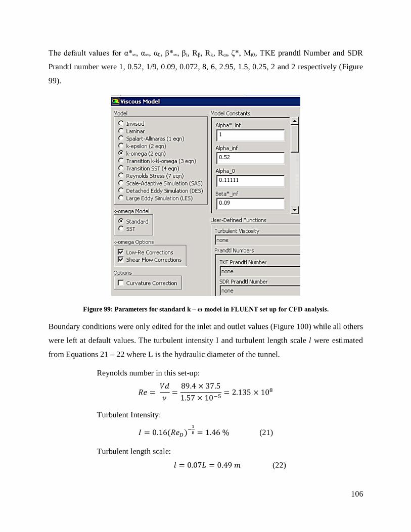
106
The default values for α*∞, α∞, α0, β*∞, βi, Rβ, Rk, Rω, ζ*, Mt0, TKE prandtl Number and SDR
Prandtl number were 1, 0.52, 1/9, 0.09, 0.072, 8, 6, 2.95, 1.5, 0.25, 2 and 2 respectively (Figure
99).
Figure 99: Parameters for standard k – ω model in FLUENT set up for CFD analysis.
Boundary conditions were only edited for the inlet and outlet values (Figure 100) while all others
were left at default values. The turbulent intensity I and turbulent length scale l were estimated
from Equations 21 – 22 where L is the hydraulic diameter of the tunnel.
Reynolds number in this set-up:
𝑅𝑒 = 𝑉𝑑𝜈
=89.4 × 37.51.57 × 10−5
= 2.135 × 10⁸
Turbulent Intensity:
𝐼 = 0.16(𝑅𝑒𝐷)−18 = 1.46 % (21)
Turbulent length scale:
𝑙 = 0.07𝐿 = 0.49 𝑚 (22)
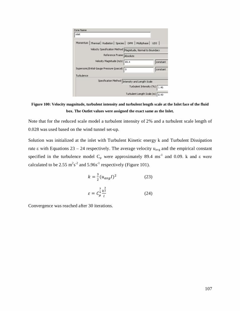
107
Figure 100: Velocity magnitude, turbulent intensity and turbulent length scale at the Inlet face of the fluid
box. The Outlet values were assigned the exact same as the Inlet.
Note that for the reduced scale model a turbulent intensity of 2% and a turbulent scale length of
0.028 was used based on the wind tunnel set-up.
Solution was initialized at the inlet with Turbulent Kinetic energy k and Turbulent Dissipation
rate ε with Equations 23 – 24 respectively. The average velocity uavg and the empirical constant
specified in the turbulence model Cµ were approximately 89.4 ms-1 and 0.09. k and ε were
calculated to be 2.55 m2s-2 and 5.96s-1 respectively (Figure 101).
𝑘 = 32
(𝑢𝑎𝑣𝑔𝐼)2 (23)
𝜀 = 𝐶𝜇34 𝑘
32
𝑙 (24)
Convergence was reached after 30 iterations.

108
Figure 101: The Solution Initialization was computed from the Inlet conditions and the velocity was set at
89.4 ms-1. Turbulent Kinetic Energy and the Specific Dissipation rate were calculated automatically from the
values of turbulent intensity and turbulent length scale.
1.4. Solution and Results
In the results section the data was represented by applying contour plot on the symmetry (Figure
102).
Figure 102: Contour plots representation of the CFD analysis on the symmetry of the boxed fluid with the tilt
angle at 70 degrees showing pressure ranging from 8.23E3 Pa (Red) to (Blue)

109
1.5. Static Structural Analysis
The second part of the analysis consisted of importing the geometry and the solution from
ANSYS FLUENT to the static structural analysis tab (Figure 103).
This time in the geometry list, the box fluid was suppressed while the other three were
unsuppressed. Material assignments were user-defined mass of 12 N, user-defined mass of 160
N, Aluminum 1061 and concrete for the PV collector, linear actuator, frame and base
respectively.
Meshing was applied to model (Figure 104) since total number of elements from FLUENT
meshing and static structural meshing of the structure should be below 512 000 elements.
Figure 103: Meshing sizing and inflation parameters used on the STS444 in Static Structural
Figure 104: View of the 105162 elements on the STS444 symmetry with no sizing and no inflation.
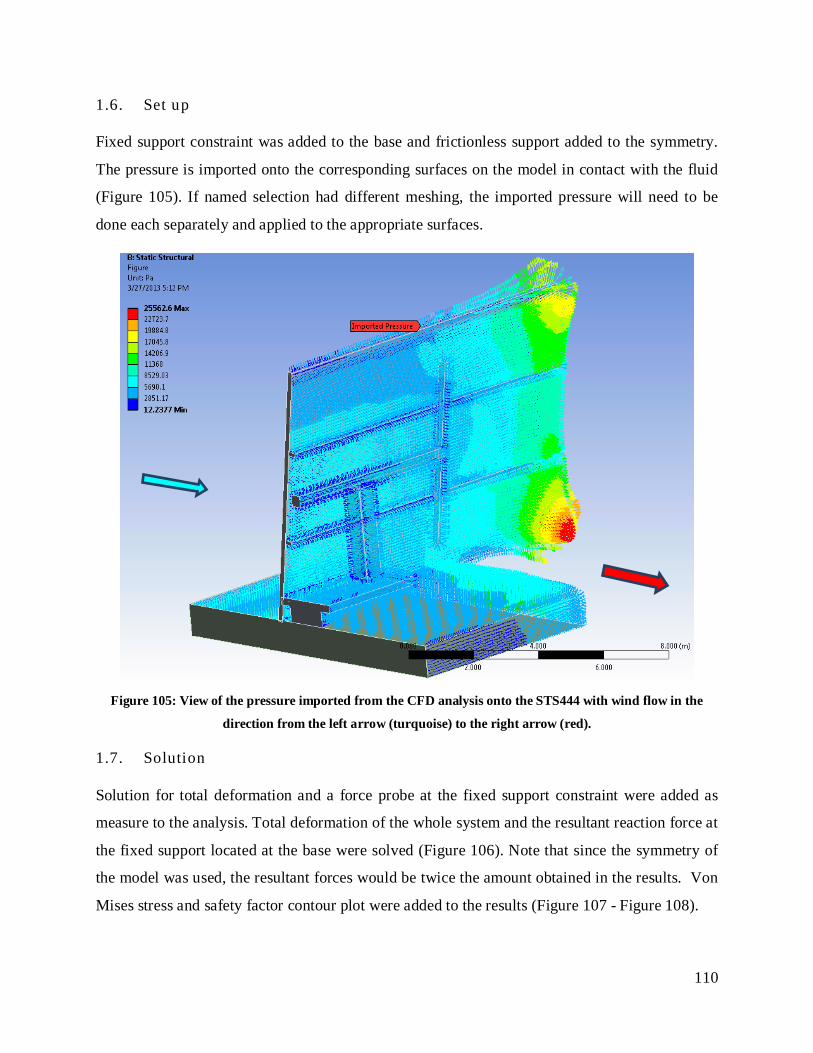
110
1.6. Set up
Fixed support constraint was added to the base and frictionless support added to the symmetry.
The pressure is imported onto the corresponding surfaces on the model in contact with the fluid
(Figure 105). If named selection had different meshing, the imported pressure will need to be
done each separately and applied to the appropriate surfaces.
Figure 105: View of the pressure imported from the CFD analysis onto the STS444 with wind flow in the
direction from the left arrow (turquoise) to the right arrow (red).
1.7. Solution
Solution for total deformation and a force probe at the fixed support constraint were added as
measure to the analysis. Total deformation of the whole system and the resultant reaction force at
the fixed support located at the base were solved (Figure 106). Note that since the symmetry of
the model was used, the resultant forces would be twice the amount obtained in the results. Von
Mises stress and safety factor contour plot were added to the results (Figure 107 - Figure 108).
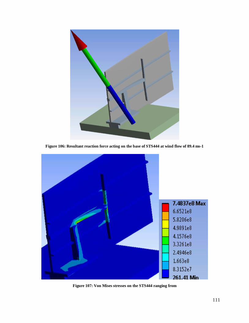
111
Figure 106: Resultant reaction force acting on the base of STS444 at wind flow of 89.4 ms-1
Figure 107: Von Mises stresses on the STS444 ranging from
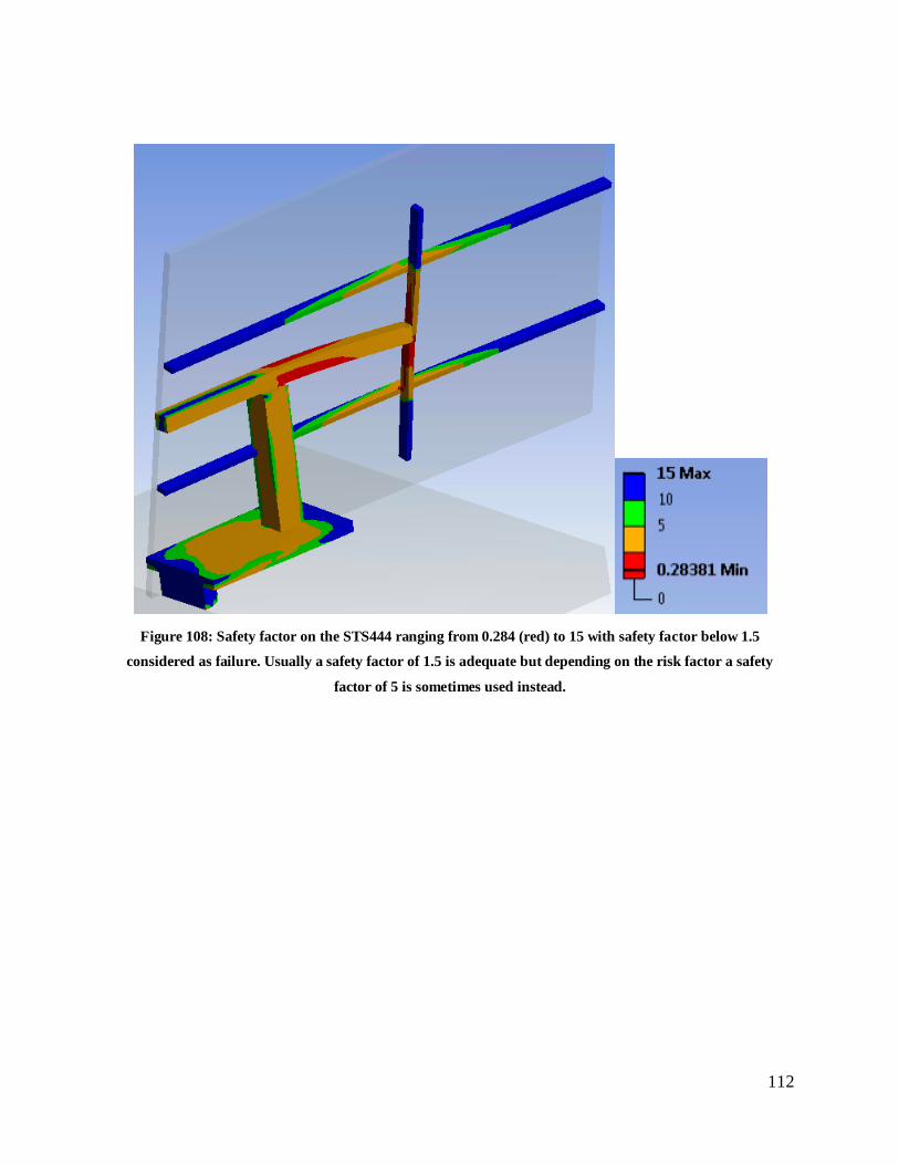
112
Figure 108: Safety factor on the STS444 ranging from 0.284 (red) to 15 with safety factor below 1.5
considered as failure. Usually a safety factor of 1.5 is adequate but depending on the risk factor a safety
factor of 5 is sometimes used instead.

113
APPENDIX D
Determination of the scaling factor in the wind tunnel testing involved numerous trial and errors
to find the matching combinations. Constraints to take into consideration before estimating the
value of the scaling factor:
i. For the scaled model to fit exactly in the side view position for the recirculating wind tunnel 24, the model must be scaled down by a factor of at least 40.
ii. Maximum velocity in wind tunnel was 60 ms-1 24.
iii. Depending on the manufacturing mode, the scaling should be matched. For the purpose of
this project, the base of the model was rapid prototyped. The maximum build dimensions of
the rapid prototyping machine are 10” x 10” x 12” (254 x 254 x 305 cm) while the minimum
recommended wall thickness is 0.06” (1.5mm).
iv. The only available estimate of the drag and lift coefficients are analytically ones. The
maximum drag or lift coefficient will be used in the force ratio to estimate maximum force.
Trial 1
Table 20: Maximum 𝐂𝐋, scaling factor and velocity of wind used for the parameters in the first trial.
Variables Trial values Analytical CL 2.5 A/m2 0.36 Full scale Ap/m2 188 Scaling factor 40 V/ms-1 60
Using Equation 4 and values listed in Table 19, the wind blockage correction at a polar angle of
80 degrees resulted in an actual wind velocity of
V′ = VA
A − 𝐴𝑝sin (90 − 𝜃)=
60(0.36)
0.36 − 188.11402 𝑠𝑖𝑛10
= 63.6 𝑚/𝑠
From Equation 3,
𝐷𝑟𝑎𝑔 = 12
× 2.5 × 1.184 × 188.11402
× 63.62 = 704 𝑁 (Too high for such a small model)

114
Trial 2
For V = 60 m/s and scaling factor 100, the calculated drag would be around 102 N (depends on
sensitivity of force sensor). Therefore to increase the force slightly, velocity could be decreased
to 45 m/s and scaling factor reduced to 90. This resulted in a maximum force of about 70 N
which was reasonable to measure.
Check for compatibility
1. Equivalent Drag on reduced model at scaling ratio 90 at speed 45 m/s:
𝐷 = 12𝐶𝐷𝜌𝐴𝑉2 = 1
2(2.5)(1.184) 188
902 (452) = 70 𝑁
2. Reynolds number:
𝑅𝑒 = 40(22.857)90(1.57×10⁻⁵)
= 6.47 × 10⁵ (turbulent)
3. Manufacturing constraints
Dimensions for rapid prototyping:
The minimum recommended wall thickness for the rapid prototyping machine is
0.060”(1.5mm), and features thinner than 0.045”(1.1mm) will likely not print. The
maximum build dimensions are 10” x 10” x 12(height)”(254x254x305mm)
The thinnest edge at scaling factor of 90 was 2.82 mm which is greater than 1.5mm
and the longest length was about 137 mm which is less than 254mm. therefore the
scaling factor of 90 is appropriate for the rapid prototype.
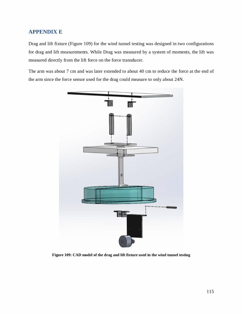
115
APPENDIX E
Drag and lift fixture (Figure 109) for the wind tunnel testing was designed in two configurations
for drag and lift measurements. While Drag was measured by a system of moments, the lift was
measured directly from the lift force on the force transducer.
The arm was about 7 cm and was later extended to about 40 cm to reduce the force at the end of
the arm since the force sensor used for the drag could measure to only about 24N.
Figure 109: CAD model of the drag and lift fixture used in the wind tunnel testing
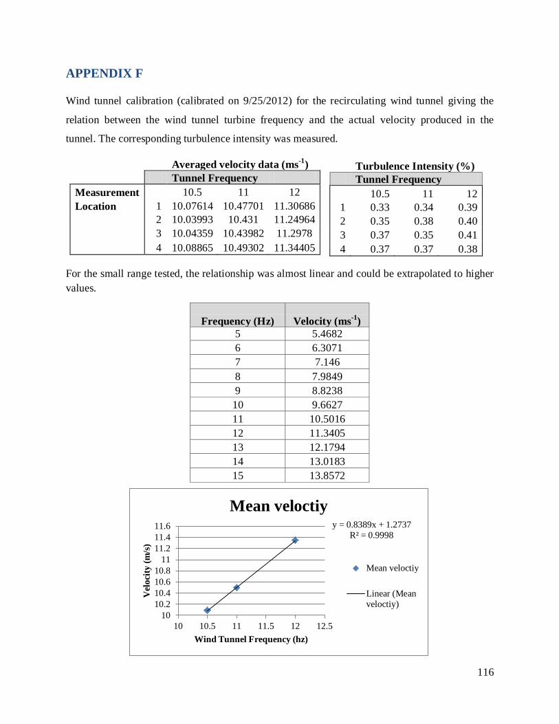
116
APPENDIX F
Wind tunnel calibration (calibrated on 9/25/2012) for the recirculating wind tunnel giving the
relation between the wind tunnel turbine frequency and the actual velocity produced in the
tunnel. The corresponding turbulence intensity was measured.
Averaged velocity data (ms-1)
Tunnel Frequency
Measurement 10.5 11 12 Location 1 10.07614 10.47701 11.30686 2 10.03993 10.431 11.24964 3 10.04359 10.43982 11.2978 4 10.08865 10.49302 11.34405
Turbulence Intensity (%)
Tunnel Frequency 10.5 11 12 1 0.33 0.34 0.39 2 0.35 0.38 0.40 3 0.37 0.35 0.41 4 0.37 0.37 0.38
For the small range tested, the relationship was almost linear and could be extrapolated to higher values.
Frequency (Hz) Velocity (ms-1) 5 5.4682 6 6.3071 7 7.146 8 7.9849 9 8.8238 10 9.6627 11 10.5016 12 11.3405 13 12.1794 14 13.0183 15 13.8572
y = 0.8389x + 1.2737 R² = 0.9998
1010.210.410.610.8
1111.211.411.6
10 10.5 11 11.5 12 12.5
Vel
ocity
(m/s
)
Wind Tunnel Frequency (hz)
Mean veloctiy
Mean veloctiy
Linear (Meanveloctiy)
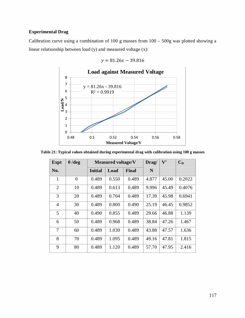
117
Experimental Drag
Calibration curve using a combination of 100 g masses from 100 – 500g was plotted showing a
linear relationship between load (y) and measured voltage (x):
𝑦 = 81.26𝑥 − 39.816
Table 21: Typical values obtained during experimental drag with calibration using 100 g masses
Expt
No.
θ /deg Measured voltage/V Drag/
N
V’ CD
Initial Load Final
1 0 0.489 0.550 0.489 4.877 45.00 0.2022
2 10 0.489 0.613 0.489 9.996 45.49 0.4076
3 20 0.489 0.704 0.489 17.39 45.98 0.6941
4 30 0.489 0.800 0.490 25.19 46.45 0.9852
5 40 0.490 0.855 0.489 29.66 46.88 1.139
6 50 0.489 0.968 0.489 38.84 47.26 1.467
7 60 0.489 1.030 0.489 43.88 47.57 1.636
8 70 0.489 1.095 0.489 49.16 47.81 1.815
9 80 0.489 1.120 0.489 57.70 47.95 2.416
y = 81.26x - 39.816 R² = 0.9919
0
1
2
3
4
5
6
7
8
0.48 0.5 0.52 0.54 0.56 0.58
Loa
d/N
Measured Voltage/V
Load against Measured Voltage
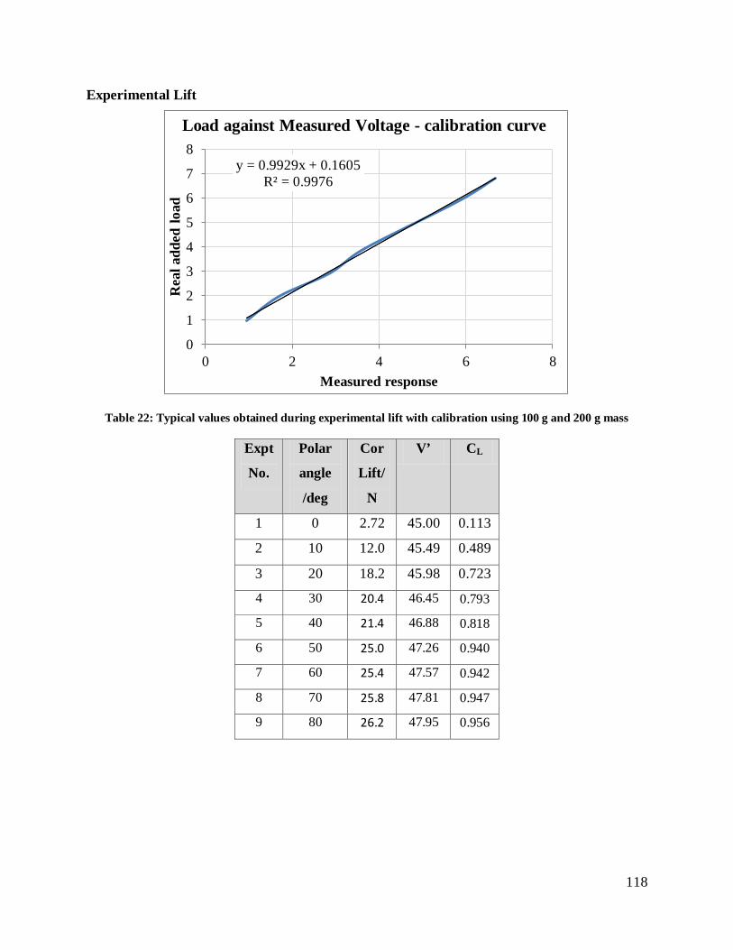
118
Experimental Lift
Table 22: Typical values obtained during experimental lift with calibration using 100 g and 200 g mass
Expt
No.
Polar
angle
/deg
Cor
Lift/
N
V’ CL
1 0 2.72 45.00 0.113
2 10 12.0 45.49 0.489
3 20 18.2 45.98 0.723
4 30 20.4 46.45 0.793
5 40 21.4 46.88 0.818
6 50 25.0 47.26 0.940
7 60 25.4 47.57 0.942
8 70 25.8 47.81 0.947
9 80 26.2 47.95 0.956
y = 0.9929x + 0.1605 R² = 0.9976
0
1
2
3
4
5
6
7
8
0 2 4 6 8
Rea
l add
ed lo
ad
Measured response
Load against Measured Voltage - calibration curve

119
APPENDIX G
When the snow was considered as a continuous mass, it was assumed that the snow was fresh
and fluffy. This implied that the individual particles all behave like independent entities with
minimum interaction with one another such as stickiness and agglomeration as seen in settled
packed snow or wet firm snow. As the panel rotates to tow the snow, the particles theoretically
slide over one another thus changing the shape and the center of mass of the snow pile. The
change in center of mass will induce an increasing moment as the difference between the panel
and pile center of masses increases. This problem involves both location and magnitude variation
of the snow load. To counter for both variations, the variable has to be added as a variable torque
with analytical calculations as to the amount of torque exerted by the snow on the panel at
different angle of rotation.
The considerations are various for profiling the snow slide:
a) The amount of snow accumulation on top of the panel set initially at 220 kgm-2 (45lb/ft2)
b) The initial shape of the snow pile
c) Determining the static and dynamic friction of the snow particles to find at what angle the
shape starts to change
d) Shape variation at each angle
e) The amount of snow that leave the panel at each angle
In order to simplify the amount of snow that fell off of the panel was cut-off at a vertical section
and represented by cross-sectional area Av (Figure 110).
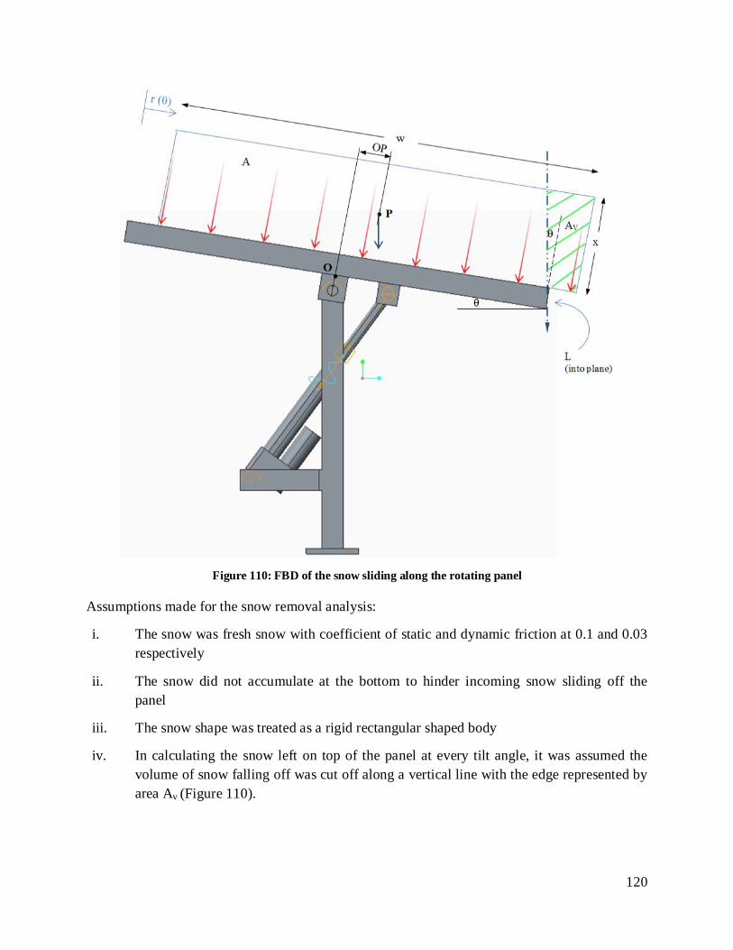
120
Figure 110: FBD of the snow sliding along the rotating panel
Assumptions made for the snow removal analysis:
i. The snow was fresh snow with coefficient of static and dynamic friction at 0.1 and 0.03 respectively
ii. The snow did not accumulate at the bottom to hinder incoming snow sliding off the panel
iii. The snow shape was treated as a rigid rectangular shaped body
iv. In calculating the snow left on top of the panel at every tilt angle, it was assumed the volume of snow falling off was cut off along a vertical line with the edge represented by area Av (Figure 110).
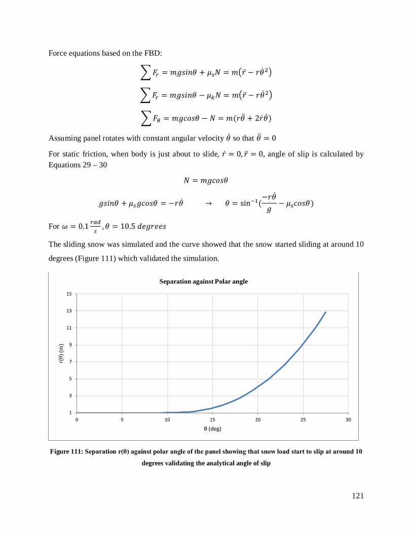
121
Force equations based on the FBD:
𝐹𝑟 = 𝑚𝑔𝑠𝑖𝑛𝜃 + 𝜇𝑠𝑁 = 𝑚 − 𝑟2
𝐹𝑟 = 𝑚𝑔𝑠𝑖𝑛𝜃 − 𝜇𝑘𝑁 = 𝑚 − 𝑟2
𝐹𝜃 = 𝑚𝑔𝑐𝑜𝑠𝜃 − 𝑁 = 𝑚(𝑟 + 2)
Assuming panel rotates with constant angular velocity so that = 0
For static friction, when body is just about to slide, = 0, = 0, angle of slip is calculated by Equations 29 – 30
𝑁 = 𝑚𝑔𝑐𝑜𝑠𝜃
𝑔𝑠𝑖𝑛𝜃 + 𝜇𝑠𝑔𝑐𝑜𝑠𝜃 = −𝑟 → 𝜃 = sin−1(−𝑟𝑔
− 𝜇𝑠𝑐𝑜𝑠𝜃)
For 𝜔 = 0.1 𝑟𝑎𝑑𝑠
,𝜃 = 10.5 𝑑𝑒𝑔𝑟𝑒𝑒𝑠
The sliding snow was simulated and the curve showed that the snow started sliding at around 10
degrees (Figure 111) which validated the simulation.
Figure 111: Separation r(θ) against polar angle of the panel showing that snow load start to slip at around 10
degrees validating the analytical angle of slip
1
3
5
7
9
11
13
15
0 5 10 15 20 25 30
r(θ)
(m)
θ (deg)
Separation against Polar angle
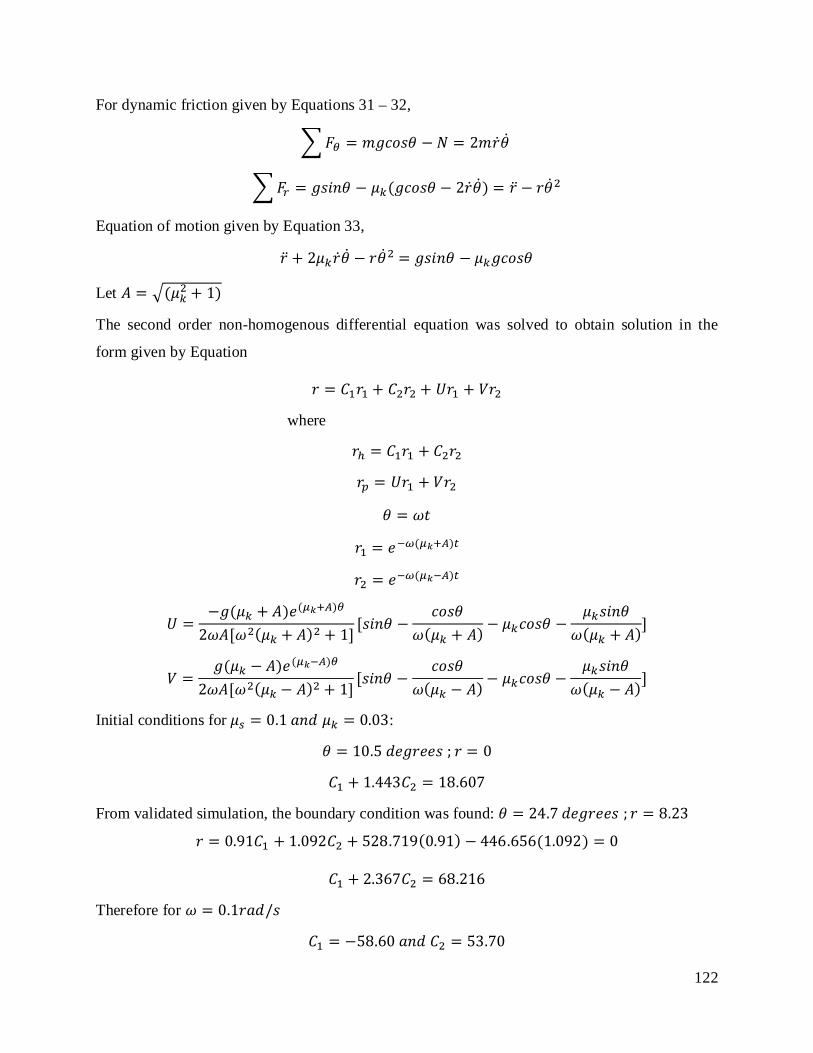
122
For dynamic friction given by Equations 31 – 32,
𝐹𝜃 = 𝑚𝑔𝑐𝑜𝑠𝜃 − 𝑁 = 2𝑚
𝐹𝑟 = 𝑔𝑠𝑖𝑛𝜃 − 𝜇𝑘(𝑔𝑐𝑜𝑠𝜃 − 2) = − 𝑟2
Equation of motion given by Equation 33,
+ 2𝜇𝑘 − 𝑟2 = 𝑔𝑠𝑖𝑛𝜃 − 𝜇𝑘𝑔𝑐𝑜𝑠𝜃
Let 𝐴 = (𝜇𝑘2 + 1)
The second order non-homogenous differential equation was solved to obtain solution in the
form given by Equation
𝑟 = 𝐶1𝑟1 + 𝐶2𝑟2 + 𝑈𝑟1 + 𝑉𝑟2
where
𝑟ℎ = 𝐶1𝑟1 + 𝐶2𝑟2
𝑟𝑝 = 𝑈𝑟1 + 𝑉𝑟2
𝜃 = 𝜔𝑡
𝑟1 = 𝑒−𝜔(𝜇𝑘+𝐴)𝑡
𝑟2 = 𝑒−𝜔(𝜇𝑘−𝐴)𝑡
𝑈 =−𝑔(𝜇𝑘 + 𝐴)𝑒(𝜇𝑘+𝐴)𝜃
2𝜔𝐴[𝜔2(𝜇𝑘 + 𝐴)2 + 1][𝑠𝑖𝑛𝜃 −
𝑐𝑜𝑠𝜃𝜔(𝜇𝑘 + 𝐴) − 𝜇𝑘𝑐𝑜𝑠𝜃 −
𝜇𝑘𝑠𝑖𝑛𝜃𝜔(𝜇𝑘 + 𝐴)]
𝑉 =𝑔(𝜇𝑘 − 𝐴)𝑒(𝜇𝑘−𝐴)𝜃
2𝜔𝐴[𝜔2(𝜇𝑘 − 𝐴)2 + 1][𝑠𝑖𝑛𝜃 −
𝑐𝑜𝑠𝜃𝜔(𝜇𝑘 − 𝐴) − 𝜇𝑘𝑐𝑜𝑠𝜃 −
𝜇𝑘𝑠𝑖𝑛𝜃𝜔(𝜇𝑘 − 𝐴)]
Initial conditions for 𝜇𝑠 = 0.1 𝑎𝑛𝑑 𝜇𝑘 = 0.03:
𝜃 = 10.5 𝑑𝑒𝑔𝑟𝑒𝑒𝑠 ; 𝑟 = 0
𝐶1 + 1.443𝐶2 = 18.607
From validated simulation, the boundary condition was found: 𝜃 = 24.7 𝑑𝑒𝑔𝑟𝑒𝑒𝑠 ; 𝑟 = 8.23
𝑟 = 0.91𝐶1 + 1.092𝐶2 + 528.719(0.91) − 446.656(1.092) = 0
𝐶1 + 2.367𝐶2 = 68.216
Therefore for 𝜔 = 0.1𝑟𝑎𝑑/𝑠
𝐶1 = −58.60 𝑎𝑛𝑑 𝐶2 = 53.70

123
For 𝜔 at 0.005 rad/s, 0.01 rad/s and 0.05 rad/s, the polar angle reached maximum before the
snow left the panel surface. Therefore since the panel would be tilted at 80 degrees, the snow
would fall mostly under gravity. The time taken for the snow to be completely removed would
be therefore a little more than the time taken for the panel to reach maximum tilt since
acceleration due to gravity is much higher at a tilt angle of 80 degrees. The only reasonable
values for angular velocities considered were those of 0.05 rad/s, 0.1 rad/s and 0.5 rad/s as listed
in Table 23.
Table 23: List of time for half cycle, total time to slide and corrected time to slide for different angular
velocities of the panel
Time to
reach 80
degrees
ω
(rad/s)
If θ > 80 deg with
constant ω
If θ < 80 deg with
constant ω
θ (deg) Time to slide θ (deg) Corrected
Time to slide
4.65 min 0.005 160 9.31min 80 > 4.65 min
2.33 min 0.01 147 4.28 min 80 > 4.28 min
27.9 sec 0.05 89.0 31.1 sec 80 > 31.1 sec
14.0 sec 0.1 39.7 6.93 sec 39.7 6.93 sec
2.79 sec 0.5 7.38 0.258 sec 7.38 0.258 sec
Based on the location of the location of the center of mass of the rigid snow, the cross-sectional
area Av of the snow sticking outside of the panel is shaved off and a new instantaneous center of
mass for the remaining snow is calculated. The torque is then calculated based on the location
and magnitude of the remaining snow on top of the panel and a torque profile was made for
different angular velocities. The torque profile was simulated and the resultant torque was
calculated on the linear actuator shaft.
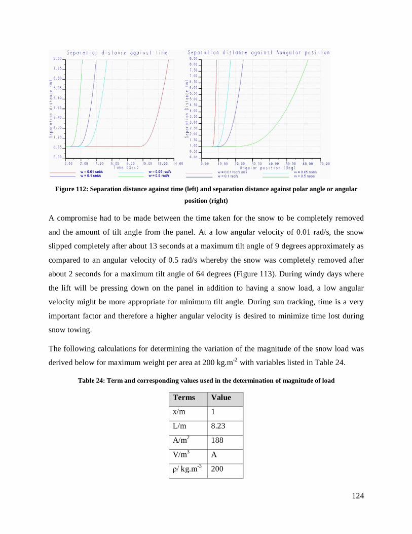
124
Figure 112: Separation distance against time (left) and separation distance against polar angle or angular
position (right)
A compromise had to be made between the time taken for the snow to be completely removed
and the amount of tilt angle from the panel. At a low angular velocity of 0.01 rad/s, the snow
slipped completely after about 13 seconds at a maximum tilt angle of 9 degrees approximately as
compared to an angular velocity of 0.5 rad/s whereby the snow was completely removed after
about 2 seconds for a maximum tilt angle of 64 degrees (Figure 113). During windy days where
the lift will be pressing down on the panel in addition to having a snow load, a low angular
velocity might be more appropriate for minimum tilt angle. During sun tracking, time is a very
important factor and therefore a higher angular velocity is desired to minimize time lost during
snow towing.
The following calculations for determining the variation of the magnitude of the snow load was
derived below for maximum weight per area at 200 kg.m-2 with variables listed in Table 24.
Table 24: Term and corresponding values used in the determination of magnitude of load
Terms Value
x/m 1
L/m 8.23
A/m2 188
V/m3 A
ρ/ kg.m-3 200

125
At angle θ:
Volume of snow left on panel 𝑉𝑠 = 𝐿[𝑥𝑤 − 𝐴𝑣(𝜃)] where
𝐴𝑣(𝜃) = 𝑟(𝜃)𝑥 +𝑥2𝑡𝑎𝑛𝜃
Total snow load on top of panel 𝑊𝑠 = 𝑉𝑠𝜌𝑔
𝑊𝑠(𝜃) = 𝜌𝑔𝐿 𝑥𝑤 − 𝑟(𝜃)𝑥 +𝑥2𝑡𝑎𝑛𝜃
Distance |𝑂𝑃| = 𝑟(𝜃)2
Torque exerted by snow which is calculated based on the offset distance from panel pivot to
center of mass of newly formed snow pile:
𝑇𝑠 = 𝑊𝑠|𝑂𝑃| =12𝑊𝑠(𝜃)𝑟(𝜃)
Conservation of power around O
𝑃 = 𝐹𝑣 = 𝑇𝜔
Axial force along the linear actuator
𝐹(𝜃) =𝑇(𝜃)𝜔(𝜃)
𝑣
For small angle θ, angular velocity ω can be assumed constant so that the profile of the force will
look somewhat similar to that of the torque profile around pin joint O multiplied by a factor v.

126
APPENDIX H
The position of the linear actuator is calculated for the design iteration 1 by using two static
cases, one when the linear actuator is fully extended and the other when it is fully retracted. A
correlation between the dimensional variables as listed in Table 25 is derived to compare the
different linear actuator available and find the optimum one.
Table 25: Terms and definition used to find optimum position of the linear actuator
Terms Definition
x Horizontal distance between point of linear actuator
and panel to the axis of rotation of panel
y Vertical distance between point of linear actuator
and frame to the axis of rotation of panel
r Half the length of panel width
H Total height of frame
θ Angle between panel and frame
a Total length of linear actuator when fully extended
b Total length of linear actuator when fully retracted
Case 1: Extended (θ = 90 deg)
Using Pythagoras law,
𝑎 = 𝑥2 + 𝑦2
Constraints: 𝑥 ≤ 𝑟 where r = 0.405 m and 𝑦 ≤ 𝐻
r
H a
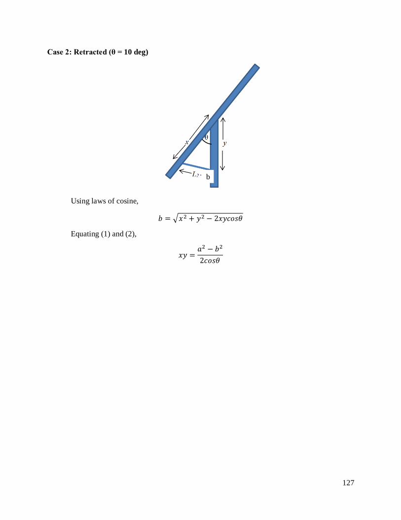
127
Case 2: Retracted (θ = 10 deg)
Using laws of cosine,
𝑏 = 𝑥2 + 𝑦2 − 2𝑥𝑦𝑐𝑜𝑠𝜃
Equating (1) and (2),
𝑥𝑦 =𝑎2 − 𝑏2
2𝑐𝑜𝑠𝜃
b

128
APPENDIX I
Analytical Approach
The following conditions applied are the maximum tilt of the collector from the horizontal at 80
degrees, extended length a, retracted length b of the linear actuator and the stroke length l as per
the manufacturer’s specifications 20 and as defined by Table 26.
Table 26: Definition of variable terms used to calculate the optimum position of the linear actuator
Term Definition
a Extended length of linear actuator
b Retracted length of linear actuator
l Stroke length of linear actuator (b-a)
x horizontal distance from bottom to upper attachment
points of the linear actuator when completely extended
y vertical distance from bottom to upper attachment
points of the linear actuator when completely extended
δ Offset distance of linear actuator attachment point on
the collector to the pivot of the collector on the frame
support.
θ Angle between panel and vertical axis
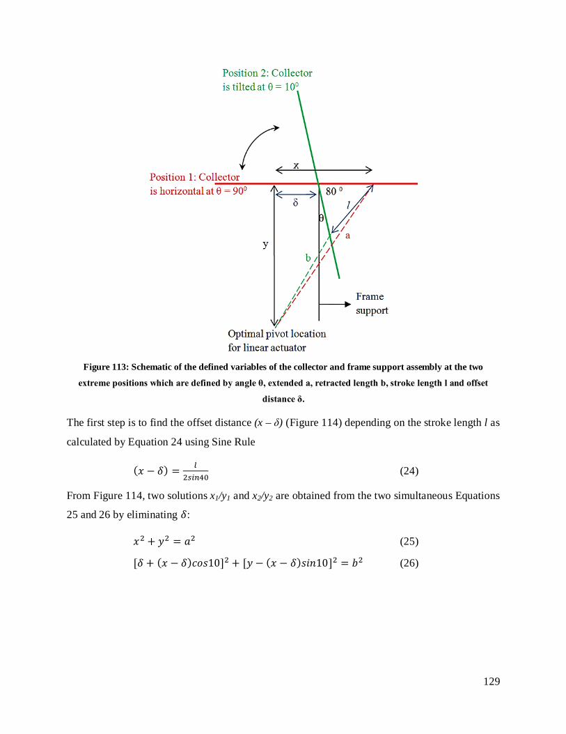
129
Figure 113: Schematic of the defined variables of the collector and frame support assembly at the two
extreme positions which are defined by angle θ, extended a, retracted length b, stroke length l and offset
distance δ.
The first step is to find the offset distance (x – δ) (Figure 114) depending on the stroke length l as
calculated by Equation 24 using Sine Rule
(𝑥 − 𝛿) = 𝑙2𝑠𝑖𝑛40
(24)
From Figure 114, two solutions x1/y1 and x2/y2 are obtained from the two simultaneous Equations
25 and 26 by eliminating 𝛿:
𝑥2 + 𝑦2 = 𝑎2 (25)
[𝛿 + (𝑥 − 𝛿)𝑐𝑜𝑠10]2 + [𝑦 − (𝑥 − 𝛿)𝑠𝑖𝑛10]2 = 𝑏2 (26)

130
Figure 114: Calculation sheet and plot of horizontal distance f(x) against x carried out in Mathcad. Equation
was iterated with f(x) = x at intersection with line h(x) = x.
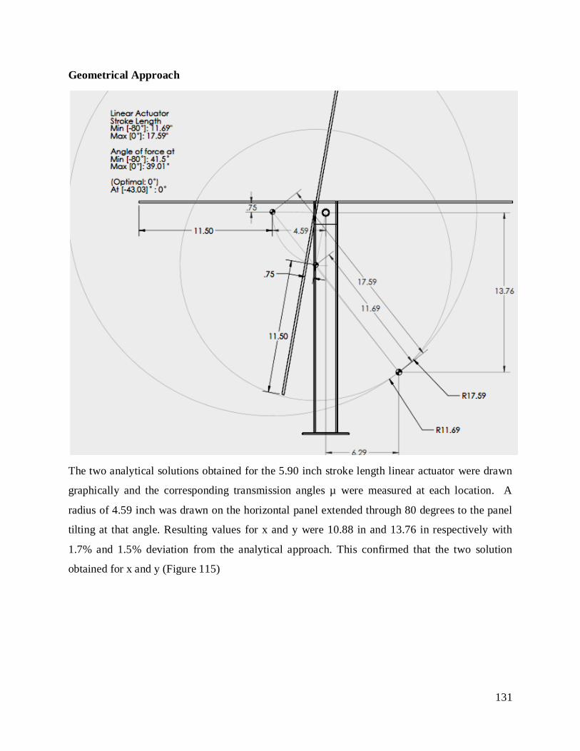
131
Geometrical Approach
The two analytical solutions obtained for the 5.90 inch stroke length linear actuator were drawn
graphically and the corresponding transmission angles µ were measured at each location. A
radius of 4.59 inch was drawn on the horizontal panel extended through 80 degrees to the panel
tilting at that angle. Resulting values for x and y were 10.88 in and 13.76 in respectively with
1.7% and 1.5% deviation from the analytical approach. This confirmed that the two solution
obtained for x and y (Figure 115)
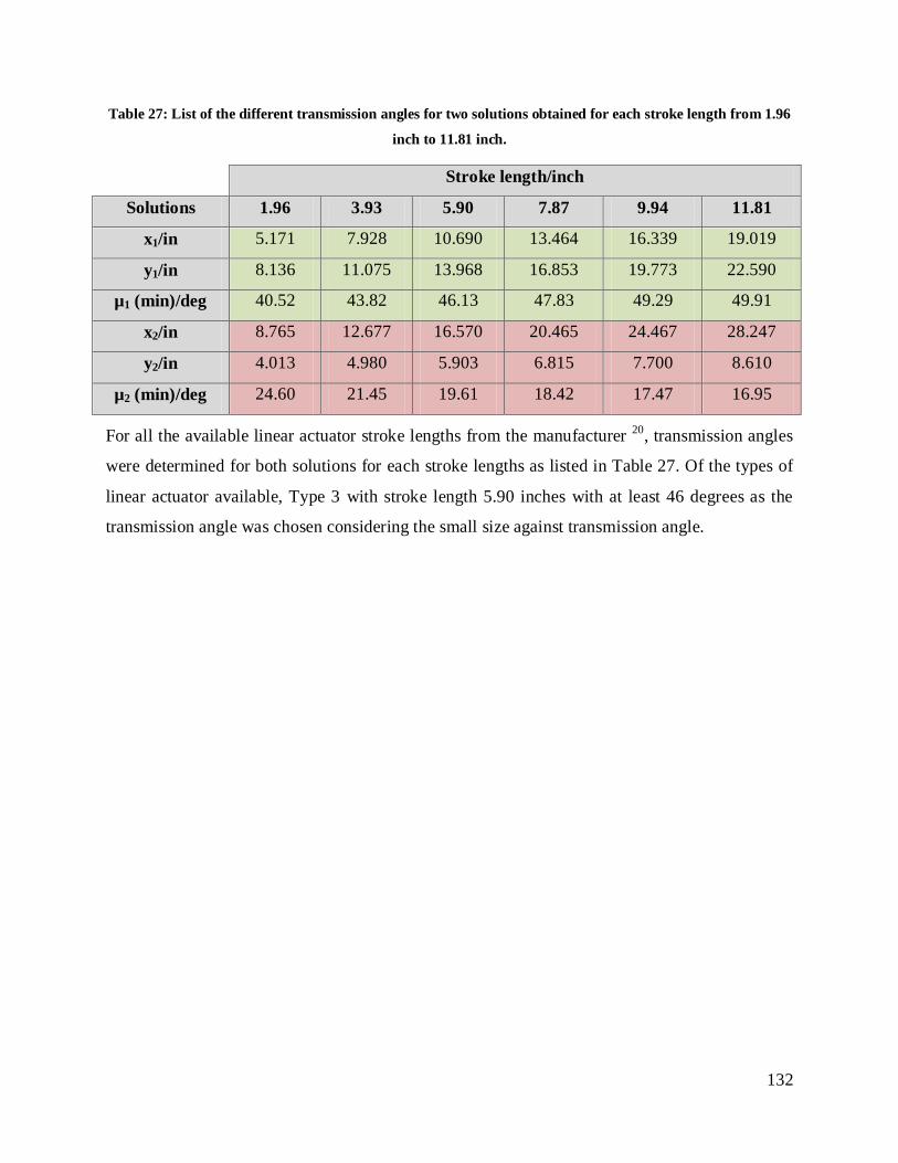
132
Table 27: List of the different transmission angles for two solutions obtained for each stroke length from 1.96
inch to 11.81 inch.
Stroke length/inch
Solutions 1.96 3.93 5.90 7.87 9.94 11.81
x1/in 5.171 7.928 10.690 13.464 16.339 19.019
y1/in 8.136 11.075 13.968 16.853 19.773 22.590
µ1 (min)/deg 40.52 43.82 46.13 47.83 49.29 49.91
x2/in 8.765 12.677 16.570 20.465 24.467 28.247
y2/in 4.013 4.980 5.903 6.815 7.700 8.610
µ2 (min)/deg 24.60 21.45 19.61 18.42 17.47 16.95
For all the available linear actuator stroke lengths from the manufacturer 20, transmission angles
were determined for both solutions for each stroke lengths as listed in Table 27. Of the types of
linear actuator available, Type 3 with stroke length 5.90 inches with at least 46 degrees as the
transmission angle was chosen considering the small size against transmission angle.
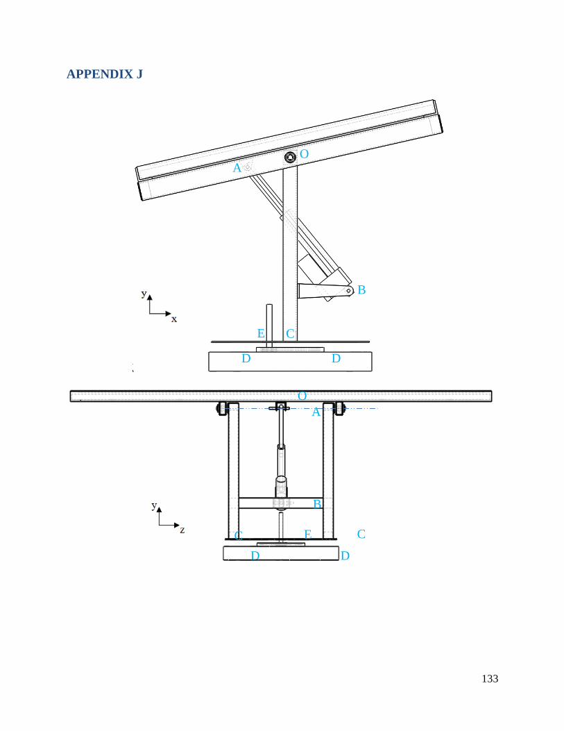
133
APPENDIX J
O A
B
C E
D D
A O
B
C C E D D
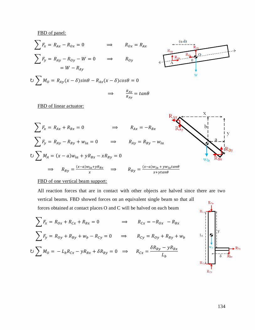
134
FBD of panel:
𝐹𝑥 = 𝑅𝐴𝑥 − 𝑅𝑂𝑥 = 0 ⟹ 𝑅𝑂𝑥 = 𝑅𝐴𝑥
𝐹𝑦 = 𝑅𝐴𝑦 − 𝑅𝑂𝑦 −𝑊 = 0 ⟹ 𝑅𝑂𝑦= 𝑊 − 𝑅𝐴𝑦
𝑀𝑂 = 𝑅𝐴𝑦(𝑥 − 𝛿)𝑠𝑖𝑛𝜃 − 𝑅𝐴𝑥(𝑥 − 𝛿)𝑐𝑜𝑠𝜃 = 0
⟹ 𝑅𝐴𝑥𝑅𝐴𝑦
= 𝑡𝑎𝑛𝜃
FBD of linear actuator:
𝐹𝑥 = 𝑅𝐴𝑥 + 𝑅𝐵𝑥 = 0 ⟹ 𝑅𝐴𝑥 = −𝑅𝐵𝑥
𝐹𝑦 = 𝑅𝐴𝑦 − 𝑅𝐵𝑦 + 𝑤𝑙𝑎 = 0 ⟹ 𝑅𝐴𝑦 = 𝑅𝐵𝑦 − 𝑤𝑙𝑎
𝑀𝐴 = (𝑥 − 𝑎)𝑤𝑙𝑎 + 𝑦𝑅𝐵𝑥 − 𝑥𝑅𝐵𝑦 = 0
⟹ 𝑅𝐵𝑦 = (𝑥−𝑎)𝑤𝑙𝑎+𝑦𝑅𝐵𝑥𝑥
⟹ 𝑅𝐵𝑦 = (𝑥−𝑎)𝑤𝑙𝑎 + 𝑦𝑤𝑙𝑎𝑡𝑎𝑛𝜃𝑥+𝑦𝑡𝑎𝑛𝜃
FBD of one vertical beam support:
All reaction forces that are in contact with other objects are halved since there are two
vertical beams. FBD showed forces on an equivalent single beam so that all
forces obtained at contact places O and C will be halved on each beam
𝐹𝑥 = 𝑅𝑂𝑥 + 𝑅𝐶𝑥 + 𝑅𝐵𝑥 = 0 ⟹ 𝑅𝐶𝑥 = −𝑅𝑂𝑥 − 𝑅𝐵𝑥
𝐹𝑦 = 𝑅𝑂𝑦 + 𝑅𝐵𝑦 + 𝑤𝑏 − 𝑅𝐶𝑦 = 0 ⟹ 𝑅𝐶𝑦 = 𝑅𝑂𝑦 + 𝑅𝐵𝑦 + 𝑤𝑏
𝑀𝑂 = − 𝐿𝑏𝑅𝐶𝑥 − 𝑦𝑅𝐵𝑥 + 𝛿𝑅𝐵𝑦 = 0 ⟹ 𝑅𝐶𝑥 =𝛿𝑅𝐵𝑦 − 𝑦𝑅𝐵𝑥
𝐿𝑏
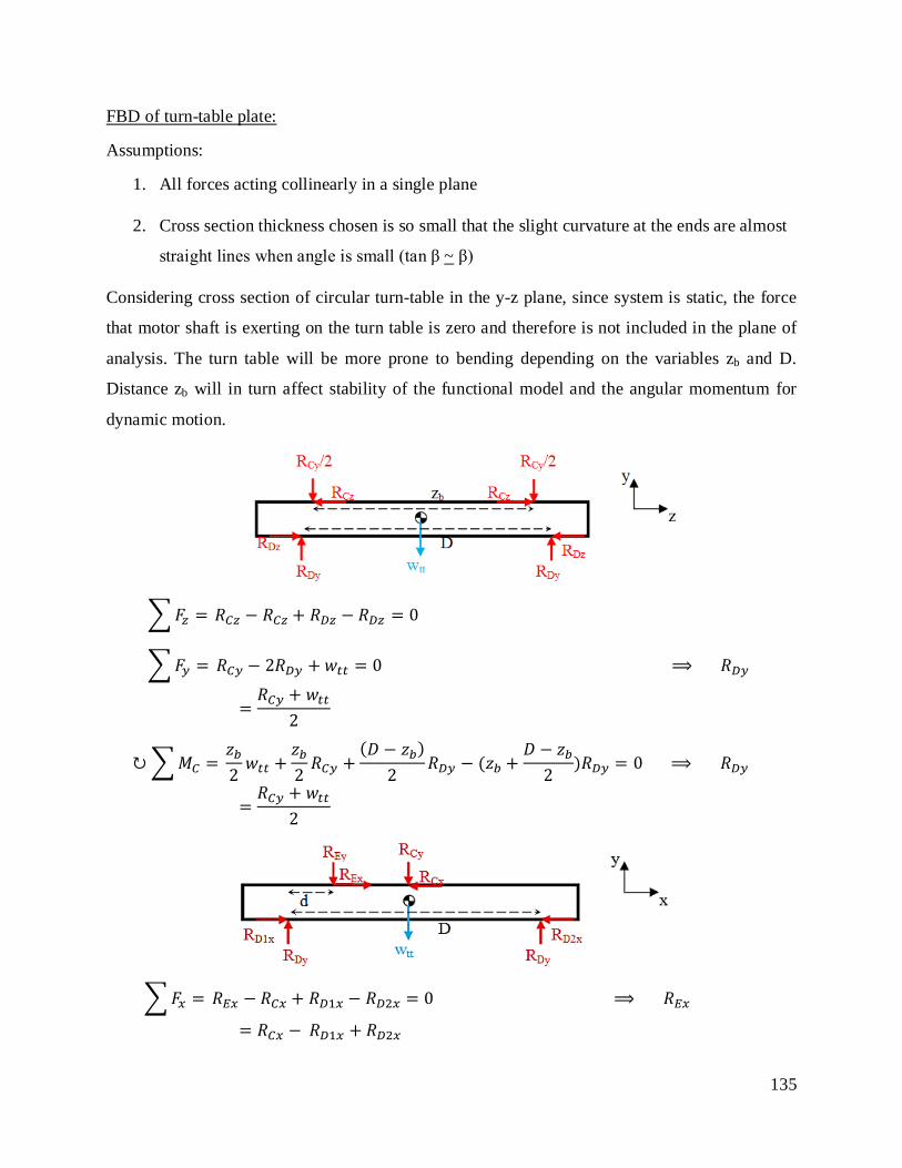
135
FBD of turn-table plate:
Assumptions:
1. All forces acting collinearly in a single plane
2. Cross section thickness chosen is so small that the slight curvature at the ends are almost
straight lines when angle is small (tan β ~ β)
Considering cross section of circular turn-table in the y-z plane, since system is static, the force
that motor shaft is exerting on the turn table is zero and therefore is not included in the plane of
analysis. The turn table will be more prone to bending depending on the variables zb and D.
Distance zb will in turn affect stability of the functional model and the angular momentum for
dynamic motion.
𝐹𝑧 = 𝑅𝐶𝑧 − 𝑅𝐶𝑧 + 𝑅𝐷𝑧 − 𝑅𝐷𝑧 = 0
𝐹𝑦 = 𝑅𝐶𝑦 − 2𝑅𝐷𝑦 + 𝑤𝑡𝑡 = 0 ⟹ 𝑅𝐷𝑦
=𝑅𝐶𝑦 + 𝑤𝑡𝑡
2
𝑀𝐶 = 𝑧𝑏2𝑤𝑡𝑡 +
𝑧𝑏2𝑅𝐶𝑦 +
(𝐷 − 𝑧𝑏)2
𝑅𝐷𝑦 − (𝑧𝑏 +𝐷 − 𝑧𝑏
2)𝑅𝐷𝑦 = 0 ⟹ 𝑅𝐷𝑦
=𝑅𝐶𝑦 + 𝑤𝑡𝑡
2
𝐹𝑥 = 𝑅𝐸𝑥 − 𝑅𝐶𝑥 + 𝑅𝐷1𝑥 − 𝑅𝐷2𝑥 = 0 ⟹ 𝑅𝐸𝑥= 𝑅𝐶𝑥 − 𝑅𝐷1𝑥 + 𝑅𝐷2𝑥
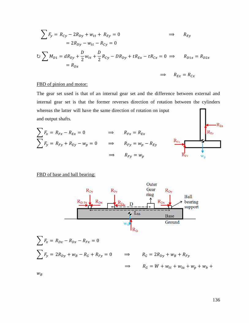
136
𝐹𝑦 = 𝑅𝐶𝑦 − 2𝑅𝐷𝑦 + 𝑤𝑡𝑡 + 𝑅𝐸𝑦 = 0 ⟹ 𝑅𝐸𝑦= 2𝑅𝐷𝑦 − 𝑤𝑡𝑡 − 𝑅𝐶𝑦 = 0
𝑀𝐷1 = 𝑑𝑅𝐸𝑦 +𝐷2𝑤𝑡𝑡 +
𝐷2𝑅𝐶𝑦 − 𝐷𝑅𝐷𝑦 + 𝑡𝑅𝐸𝑥 − 𝑡𝑅𝐶𝑥 = 0 ⟹ 𝑅𝐷1𝑥 = 𝑅𝐷2𝑥
= 𝑅𝐷𝑥
⟹ 𝑅𝐸𝑥 = 𝑅𝐶𝑥
FBD of pinion and motor:
The gear set used is that of an internal gear set and the difference between external and
internal gear set is that the former reverses direction of rotation between the cylinders
whereas the latter will have the same direction of rotation on input
and output shafts.
𝐹𝑥 = 𝑅𝐹𝑥 − 𝑅𝐸𝑥 = 0 ⟹ 𝑅𝐹𝑥 = 𝑅𝐸𝑥
𝐹𝑦 = 𝑅𝐹𝑦 + 𝑅𝐸𝑦 − 𝑤𝑝 = 0 ⟹ 𝑅𝐹𝑦 = 𝑤𝑝 − 𝑅𝐸𝑦
⟹ 𝑅𝐹𝑦 = 𝑤𝑝
FBD of base and ball bearing:
𝐹𝑥 = 𝑅𝐷𝑥 − 𝑅𝐷𝑥 − 𝑅𝐹𝑥 = 0
𝐹𝑦 = 2𝑅𝐷𝑦 + 𝑤𝐵 − 𝑅𝐺 + 𝑅𝐹𝑦 = 0 ⟹ 𝑅𝐺 = 2𝑅𝐷𝑦 + 𝑤𝐵 + 𝑅𝐹𝑦
⟹ 𝑅𝐺 = 𝑊 + 𝑤𝑡𝑡 + 𝑤𝑙𝑎 + 𝑤𝑝 + 𝑤𝑏 +𝑤𝐵
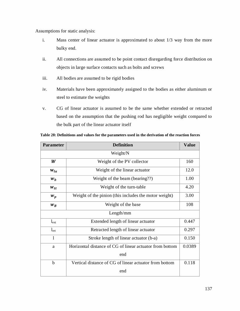
137
Assumptions for static analysis:
i. Mass center of linear actuator is approximated to about 1/3 way from the more
bulky end.
ii. All connections are assumed to be point contact disregarding force distribution on
objects in large surface contacts such as bolts and screws
iii. All bodies are assumed to be rigid bodies
iv. Materials have been approximately assigned to the bodies as either aluminum or
steel to estimate the weights
v. CG of linear actuator is assumed to be the same whether extended or retracted
based on the assumption that the pushing rod has negligible weight compared to
the bulk part of the linear actuator itself
Table 28: Definitions and values for the parameters used in the derivation of the reaction forces
Parameter Definition Value
Weight/N
𝑾 Weight of the PV collector 160
𝐰𝒍𝒂 Weight of the linear actuator 12.0
𝒘𝒃 Weight of the beam (bearing??) 1.00
𝒘𝒕𝒕 Weight of the turn-table 4.20
𝒘𝒑 Weight of the pinion (this includes the motor weight) 3.00
𝒘𝑩 Weight of the base 108
Length/mm
lext Extended length of linear actuator 0.447
lret Retracted length of linear actuator 0.297
l Stroke length of linear actuator (b-a) 0.150
a Horizontal distance of CG of linear actuator from bottom
end
0.0389
b Vertical distance of CG of linear actuator from bottom
end
0.118
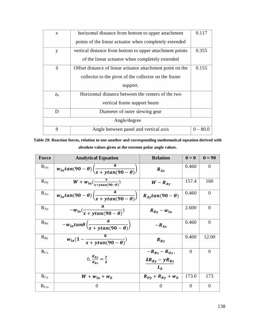
138
x horizontal distance from bottom to upper attachment
points of the linear actuator when completely extended
0.117
y vertical distance from bottom to upper attachment points
of the linear actuator when completely extended
0.355
δ Offset distance of linear actuator attachment point on the
collector to the pivot of the collector on the frame
support.
0.155
zb Horizontal distance between the centers of the two
vertical frame support beam
D Diameter of outer slewing gear
Angle/degree
θ Angle between panel and vertical axis 0 – 80.0
Table 29: Reaction forces, relation to one another and corresponding mathematical equation derived with
absolute values given at the extreme polar angle values.
Force Analytical Equation Relation θ = 0 θ = 90
ROx 𝒘𝒍𝒂𝒕𝒂𝒏(𝟗𝟎 − 𝜽) 𝐚
𝒙 + 𝒚𝒕𝒂𝒏(𝟗𝟎 − 𝜽) 𝑹𝑨𝒙 0.460 0
ROy 𝑾 + 𝒘𝒍𝒂( 𝐚𝒙+𝒚𝒕𝒂𝒏(𝟗𝟎−𝜽)
) 𝑾−𝑹𝑨𝒚 157.4 160
RAx 𝒘𝒍𝒂𝒕𝒂𝒏(𝟗𝟎 − 𝜽) 𝐚
𝒙 + 𝒚𝒕𝒂𝒏(𝟗𝟎 − 𝜽) 𝑹𝑨𝒚𝒕𝒂𝒏(𝟗𝟎 − 𝜽) 0.460 0
RAy −𝒘𝒍𝒂(𝐚
𝒙 + 𝒚𝒕𝒂𝒏(𝟗𝟎 − 𝜽)) 𝑹𝑩𝒚 − 𝒘𝒍𝒂 2.600 0
RBx −𝒘𝒍𝒂𝒕𝒂𝒏𝜽 𝐚
𝒙 + 𝒚𝒕𝒂𝒏(𝟗𝟎 − 𝜽) −𝑹𝑨𝒙 0.460 0
RBy 𝒘𝒍𝒂(𝟏 −𝐚
𝒙 + 𝒚𝒕𝒂𝒏(𝟗𝟎 − 𝜽)) 𝑹𝑩𝒚 9.400 12.00
RCx
0, 𝑹𝑩𝒚𝑹𝑩𝒙
= 𝒚𝜹
−𝑹𝑩𝒙 − 𝑹𝑶𝒙 , 𝜹𝑹𝑩𝒚 − 𝒚𝑹𝑩𝒙
𝑳𝒃
0 0
RCy 𝑾 + 𝒘𝒍𝒂 + 𝒘𝒃 𝑹𝑶𝒚 + 𝑹𝑩𝒚 + 𝒘𝒃 173.0 173
RCz, 0 0 0 0
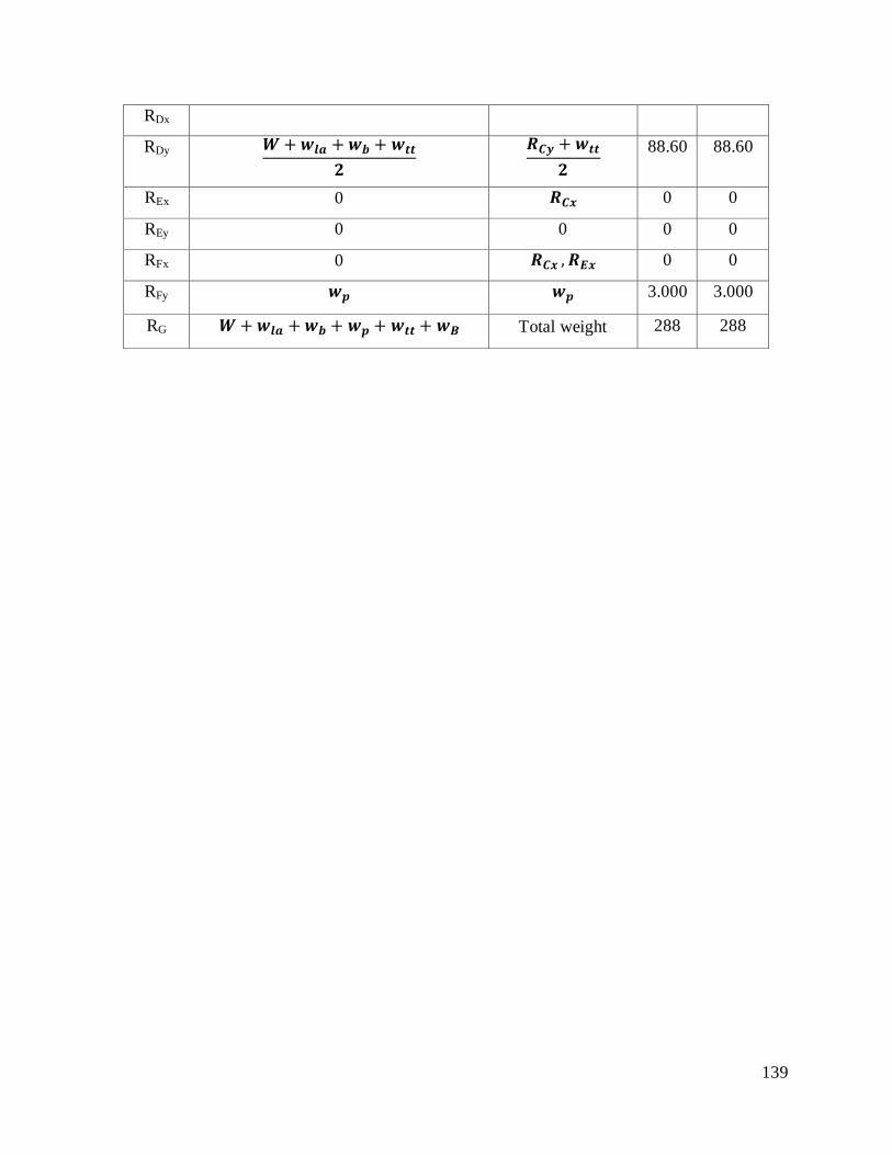
139
RDx
RDy 𝑾 + 𝒘𝒍𝒂 + 𝒘𝒃 + 𝒘𝒕𝒕
𝟐
𝑹𝑪𝒚 + 𝒘𝒕𝒕
𝟐
88.60 88.60
REx 0 𝑹𝑪𝒙 0 0
REy 0 0 0 0
RFx 0 𝑹𝑪𝒙 ,𝑹𝑬𝒙 0 0
RFy 𝒘𝒑 𝒘𝒑 3.000 3.000
RG 𝑾 + 𝒘𝒍𝒂 + 𝒘𝒃 + 𝒘𝒑 + 𝒘𝒕𝒕 + 𝒘𝑩 Total weight 288 288
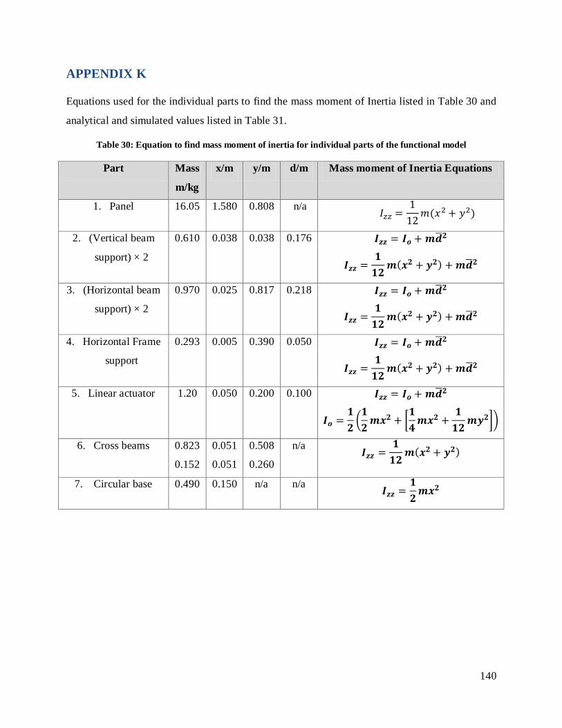
140
APPENDIX K
Equations used for the individual parts to find the mass moment of Inertia listed in Table 30 and
analytical and simulated values listed in Table 31.
Table 30: Equation to find mass moment of inertia for individual parts of the functional model
Part Mass
m/kg
x/m y/m d/m Mass moment of Inertia Equations
1. Panel 16.05 1.580 0.808 n/a 𝐼𝑧𝑧 =1
12𝑚(𝑥2 + 𝑦2)
2. (Vertical beam
support) × 2
0.610 0.038 0.038 0.176 𝑰𝒛𝒛 = 𝑰𝒐 + 𝒎𝒅𝟐
𝑰𝒛𝒛 =𝟏𝟏𝟐
𝒎(𝒙𝟐 + 𝒚𝟐) + 𝒎𝒅𝟐
3. (Horizontal beam
support) × 2
0.970 0.025 0.817 0.218 𝑰𝒛𝒛 = 𝑰𝒐 + 𝒎𝒅𝟐
𝑰𝒛𝒛 =𝟏𝟏𝟐
𝒎(𝒙𝟐 + 𝒚𝟐) + 𝒎𝒅𝟐
4. Horizontal Frame
support
0.293 0.005 0.390 0.050 𝑰𝒛𝒛 = 𝑰𝒐 + 𝒎𝒅𝟐
𝑰𝒛𝒛 =𝟏𝟏𝟐
𝒎(𝒙𝟐 + 𝒚𝟐) + 𝒎𝒅𝟐
5. Linear actuator 1.20 0.050 0.200 0.100 𝑰𝒛𝒛 = 𝑰𝒐 + 𝒎𝒅𝟐
𝑰𝒐 =𝟏𝟐𝟏𝟐𝒎𝒙𝟐 +
𝟏𝟒𝒎𝒙𝟐 +
𝟏𝟏𝟐
𝒎𝒚𝟐
6. Cross beams 0.823
0.152
0.051
0.051
0.508
0.260
n/a 𝑰𝒛𝒛 =𝟏𝟏𝟐
𝒎(𝒙𝟐 + 𝒚𝟐)
7. Circular base 0.490 0.150 n/a n/a 𝑰𝒛𝒛 =𝟏𝟐𝒎𝒙𝟐

141
Table 31: Mass moment of Inertia for individual parts in the functional model obtained analytically and by
simulation
Part
Mass Moment of Inertia
(Izz/kgm2)
Calculations Simulated
Panel 4.2121 4.6618
(Vertical beam support)
x2
0.0381 0.0004
(Horizontal beam
support) x2
0.2002 0.1092
Horizontal Frame
support
0.0044 0.0030
Linear actuator 0.0031 0.0050
Cross beams 0.0188 0.0208
Circular base 0.0055 0.0056
Total 4.4822 4.8058
Note:
1. In calculations of mass moment of inertia for PV collector, supporting welded beams were not taken into account unlike in the Solidworks simulations
2. The vertical beams and horizontal beams calculations were an overestimate since in reality they were hollow while in the calculations they were treated as filled.
3. Center of gravity for linear actuator in calculations was placed one third of total length in all directions from the base
4. Mass moment of inertia for linear actuator in Solidworks was taken when linear actuator was completely vertical with center of gravity at one third distance of total length in all directions from the base.
5. Both results for mass moment of inertia by calculation and Solidworks simulations do not include miscellaneous items such as the electric box, bolts, screws and other items that will add slightly to the mass moment of inertia.
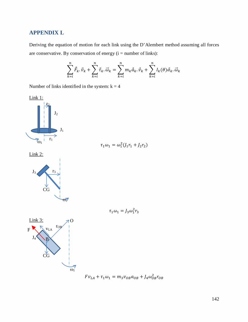
142
APPENDIX L
Deriving the equation of motion for each link using the D’Alembert method assuming all forces
are conservative. By conservation of energy (i = number of links):
𝑘 . 𝑘
𝑛
𝑘=𝑖
+ 𝜏𝑘 .𝜔 𝑘
𝑛
𝑘=𝑖
= 𝑚𝑘𝑘 . 𝑘
𝑛
𝑘=𝑖
+ 𝐼𝑘(𝜃)𝑘 .𝜔 𝑘
𝑛
𝑘=𝑖
Number of links identified in the system: k = 4
Link 1:
𝜏1𝜔1 = 𝜔12(𝐽1𝑟1 + 𝐽2𝑟2)
Link 2:
𝜏1𝜔1 = 𝐽3𝜔12𝑟3
Link 3:
𝐹𝑣𝐿𝐴 + 𝜏1𝜔1 = 𝑚3𝑣𝑂𝐵𝑎𝑂𝐵 + 𝐽4𝜔𝑂𝐵2 𝑟𝑂𝐵
ω1
J1
J2
r1
r2
CG
r3
ω1
J3
CG
rOB
ω1
J4
F vLA
B
O
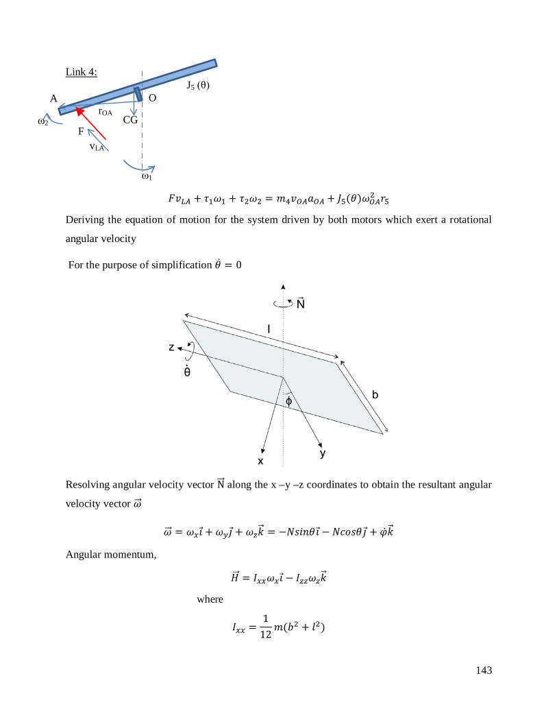
143
Link 4:
𝐹𝑣𝐿𝐴 + 𝜏1𝜔1 + 𝜏2𝜔2 = 𝑚4𝑣𝑂𝐴𝑎𝑂𝐴 + 𝐽5(𝜃)𝜔𝑂𝐴2 𝑟5
Deriving the equation of motion for the system driven by both motors which exert a rotational
angular velocity
For the purpose of simplification = 0
Resolving angular velocity vector N along the x –y –z coordinates to obtain the resultant angular
velocity vector 𝜔
𝜔 = 𝜔𝑥𝚤 + 𝜔𝑦𝚥 + 𝜔𝑧𝑘 = −𝑁𝑠𝑖𝑛𝜃𝚤 − 𝑁𝑐𝑜𝑠𝜃𝚥 + 𝑘
Angular momentum,
𝐻 = 𝐼𝑥𝑥𝜔𝑥𝚤 − 𝐼𝑧𝑧𝜔𝑧𝑘
where
𝐼𝑥𝑥 =1
12𝑚(𝑏2 + 𝑙2)
CG
ω1
J5 (θ)
F
A
ω2
vLA
O rOA

144
𝐼𝑧𝑧 =1
12𝑚𝑏2
Kinetic energy,
𝑇 =12𝜔 .𝐻
Assuming potential energy negligible,
𝑉 = 0
Lagrangian Equation,
𝐿 = 𝑇 − 𝑉
𝑑𝑑𝑡
𝜕𝐿𝜕𝑖
−𝜕𝐿𝜕𝑞𝑖
= 𝑄𝑖𝑛𝑐 𝑤ℎ𝑒𝑟𝑒 𝑖 = 1,2, …𝑛
Assuming system is frictionless so that forces are conservative,
𝑑𝑑𝑡
𝜕𝐿𝜕𝑖
−𝜕𝐿𝜕𝑞𝑖
= 0
Partial derivatives,
𝑑𝑑𝑡
𝜕𝐿𝜕
=1
12𝑚𝑏2
𝜕𝐿𝜕𝜑
=1
12𝑚(𝑏2 + 𝑙2)𝑁2𝑠𝑖𝑛𝜑𝑐𝑜𝑠𝜑
Therefore Equation of motion,
𝑚𝑏2 − 𝑚(𝑏2 + 𝑙2)𝑁2𝑠𝑖𝑛𝜑𝑐𝑜𝑠𝜑 = 0
It turns out that equation above would only work if:
i. It can be seen that if a rotation N is imposed, since Izz is changing the total energy will not be conserved since there will be coriolis effects and change in inertia if in addition angular velocity was imposed.
ii. The change in inertia can be solved by introducing a rotation matrix that would transform the axes of rotation to change from one plane to another plane. However coriolis effect will still need to be taken into consideration with imposed rotation.
iii. Therefore the above equation would only work in the stall position where 𝜑 = 90

145
iv. In the simplified version of 𝜑 = 90
The full analysis of the motion was a little more complex and was beyond the scope of this project. Therefore in the simplified version, the equation of motion would be based on the Euler Equations:
Euler’s Equations
𝑀𝑥 = 𝐼𝑥𝑥𝑥 − (𝐼𝑦𝑦 − 𝐼𝑧𝑧)𝜔𝑦𝜔𝑧
𝑀𝑦 = 𝐼𝑦𝑦𝑦 − (𝐼𝑧𝑧 − 𝐼𝑥𝑥)𝜔𝑧𝜔𝑥
𝑀𝑧 = 𝐼𝑧𝑧𝑧 − (𝐼𝑥𝑥 − 𝐼𝑦𝑦)𝜔𝑥𝜔𝑦
Where if rotation is considered in x – axis only with constant angular velocity and at polar angle of 0 degree, equation of motion will simply be:
𝑀 = 𝐼𝑥𝑥𝑥

146
APPENDIX M
//Arduino code for solar tracker //Two light sensors, wind sensor, load sensor #define sensitivity 100 //sensitivity of the tracker (lower value -> higher sensitivity) #define LA_PWM 100 //PWM output for linear actuator (255 -> full power) #define BM_PWM 100 //PWM output for base motor (255 -> full power) #define LA_extended_value 840 //Feedback value from LA when extended (panel at 0 degree) #define LA_retracted_value 180 //Feedback value from LA when retracted (panel at 80 degree) #define wind_sensor_limit 500 #define load_sensor_limit 400 #define time_limit 10000 //Time limit to reset wind_gust_count to 0 /////////////////////////////////////////////////////////////////////////////////// //Pin assignment & initialization /////////////////////////////////////////////////////////////////////////////////// int LA_out_A = 3; //Linear actuator output A int LA_out_B = 2; //Linear actuator output B int BM_out_A = 4; //Base motor output A int BM_out_B = 5; //Base motor output B int wind_state = 0; int wind_gust_count = 0; int last_wind_state = 0; unsigned long previousMillis = 0; unsigned long currentMillis = 0; /////////////////////////////////////////////////////////////////////////////////// //Setup /////////////////////////////////////////////////////////////////////////////////// void setup() pinMode(LA_out_A, OUTPUT); pinMode(LA_out_B, OUTPUT); pinMode(BM_out_A, OUTPUT); pinMode(BM_out_B, OUTPUT); Serial.begin(9600); /////////////////////////////////////////////////////////////////////////////////// //Loop /////////////////////////////////////////////////////////////////////////////////// void loop() //Tracking///////////////////////////////////////////////////////////////////////// int LA_error = (analogRead(A0) - (analogRead(A1))); int BM_error = (analogRead(A2) - (analogRead(A3))); if ((LA_error > sensitivity) && (analogRead(A6) > LA_retracted_value)) analogWrite(LA_out_A, 0); analogWrite(LA_out_B, LA_PWM); else if ((LA_error < -(sensitivity)) && (analogRead(A6) < LA_extended_value)) analogWrite(LA_out_A, LA_PWM); analogWrite(LA_out_B, 0); else analogWrite(LA_out_A, 0); analogWrite(LA_out_B, 0);
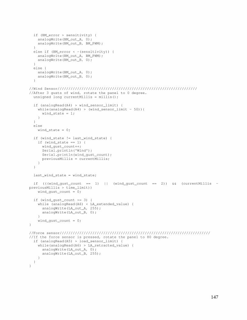
147
if (BM_error > sensitivity) analogWrite(BM_out_A, 0); analogWrite(BM_out_B, BM_PWM); else if (BM_error < -(sensitivity)) analogWrite(BM_out_A, BM_PWM); analogWrite(BM_out_B, 0); else analogWrite(BM_out_A, 0); analogWrite(BM_out_B, 0); //Wind Sensor//////////////////////////////////////////////////////////////// //After 3 gusts of wind, rotate the panel to 0 degree. unsigned long currentMillis = millis(); if (analogRead(A4) > wind_sensor_limit) while(analogRead(A4) > (wind_sensor_limit - 50)) wind_state = 1; else wind_state = 0; if (wind_state != last_wind_state) if (wind_state == 1) wind_gust_count++; Serial.println("Wind"); Serial.println(wind_gust_count); previousMillis = currentMillis; last_wind_state = wind_state; if (((wind_gust_count == 1) || (wind_gust_count == 2)) && (currentMillis - previousMillis > time_limit)) wind_gust_count = 0; if (wind_gust_count >= 3) while (analogRead(A6) < LA_extended_value) analogWrite(LA_out_A, 255); analogWrite(LA_out_B, 0); wind_gust_count = 0; //Force sensor///////////////////////////////////////////////////////////////////// //If the force sensor is pressed, rotate the panel to 80 degree. if (analogRead(A5) > load_sensor_limit) while(analogRead(A6) > LA_retracted_value) analogWrite(LA_out_A, 0); analogWrite(LA_out_B, 255);

148
APPENDIX N
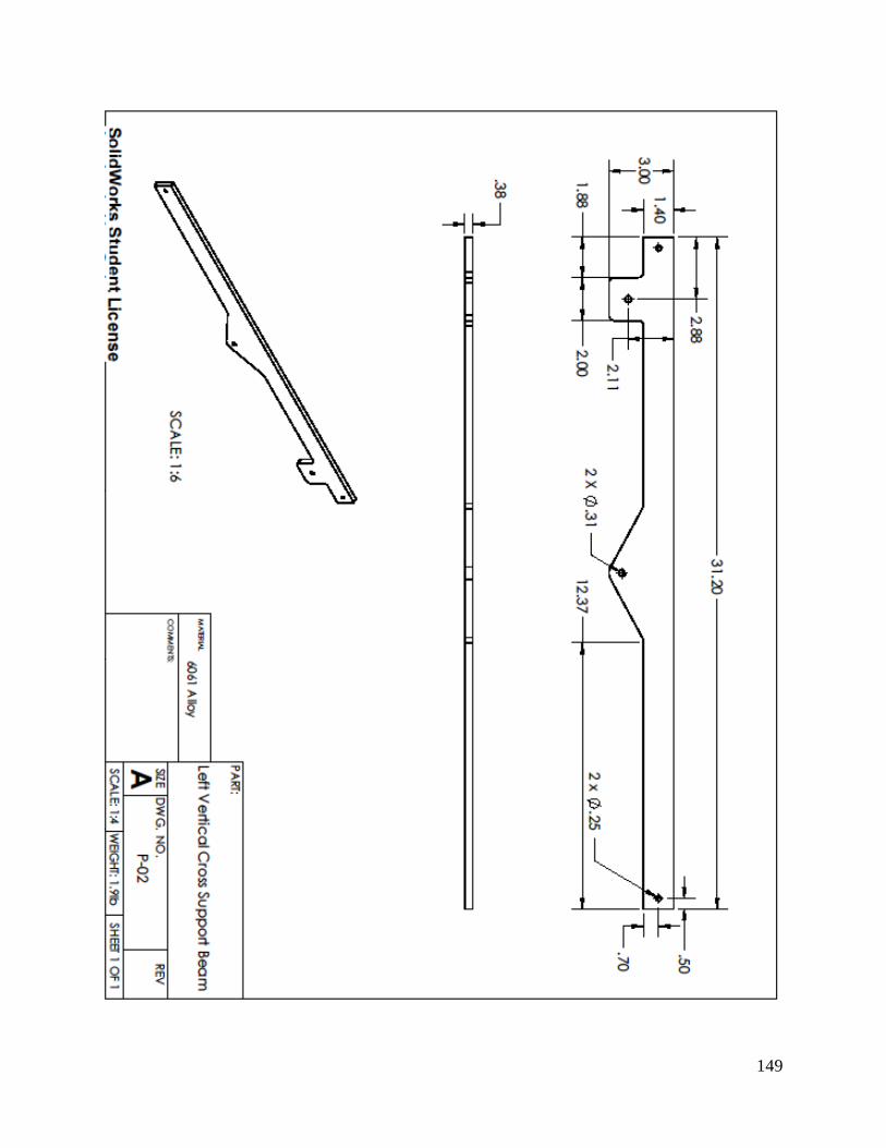
149
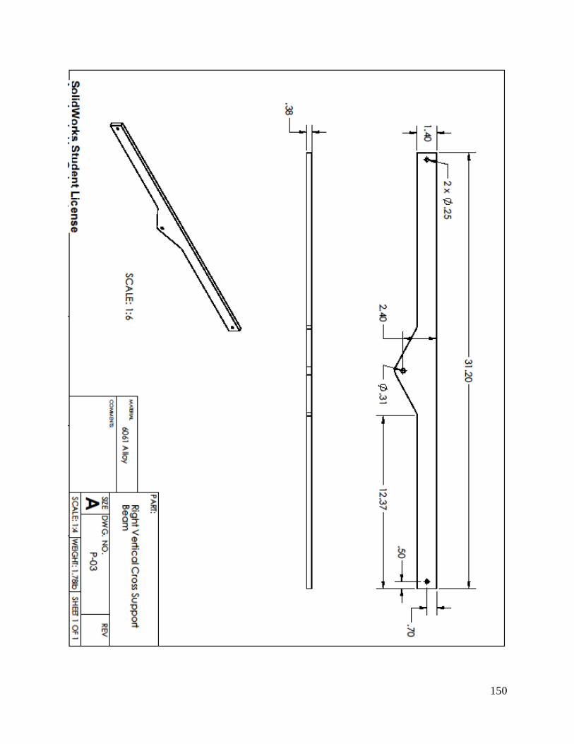
150
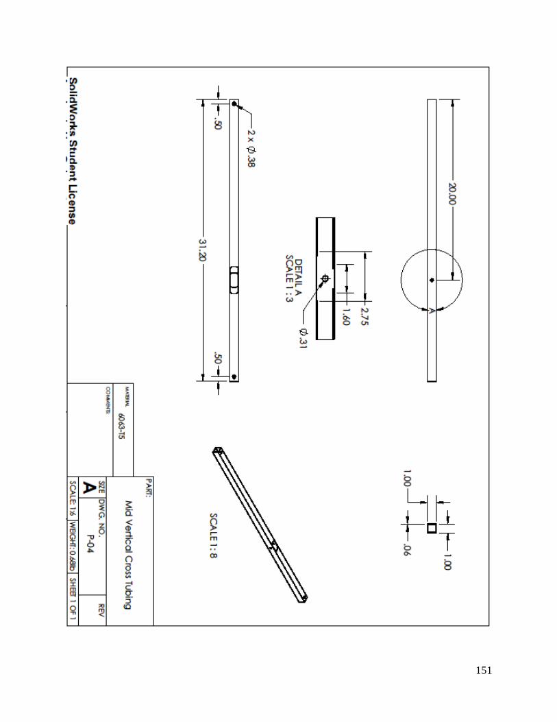
151

152
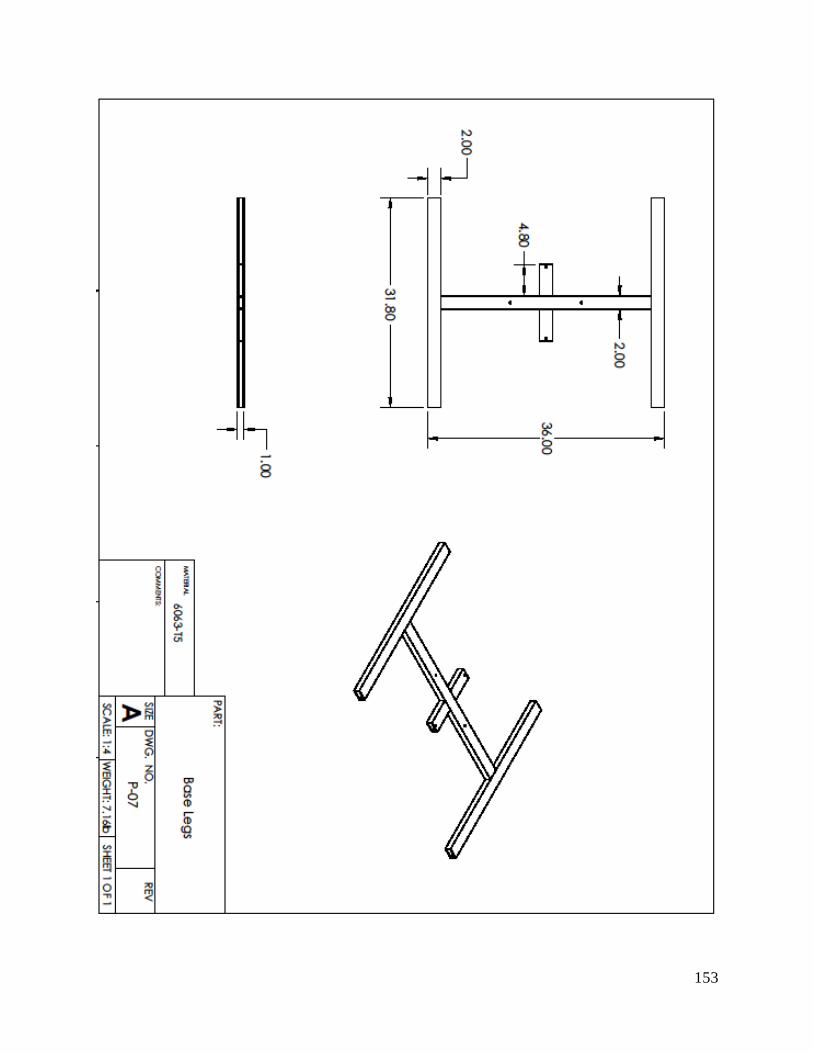
153

154
155
REFERENCES
[1] H. Sterling Burnett, Solar Power Prospects. National Center for Policy Analysis; Policy Report No.
334 May (2011). http://www.ncpa.org/pdfs/st334.pdf
[2] U.S. Energy Information Administration. Annual Energy Review 2011. DOE/EIA-0384(2011)
(September 2012). http://www.eia.gov/totalenergy/data/annual/pdf/aer.pdf
[3] U.S. Energy Information Administration. Annual Energy Review 2011. DOE/EIA-0384(2010)
(October 2011). http://www.eia.gov/totalenergy/data/annual/archive/038410.pdf
[4] Stefan Reichelstein, The Prospects for Cost-Competitive Solar PV Power”.
http://www.gsb.stanford.edu/news/headlines/Reichelstein-solar-2012.html
[5] H. Mousazadeh et al., A review of principle and sun tracking methods for maximizing solar systems
output, Renewable and Sustainable Energy Reviews 13 (2009) 1800–1818.
[6] Salah Abdallah, The effect of using sun tracking systems on the voltage–current characteristics and
power generation of flat plate photovoltaics. Energy Conversion and Management. 45 (2004) 1671–1679
[7] Mehleri, E.D., P.L. Zervas, H. Sarimveis, J.A. Palyvos, and N.C. Markatos. Determination of the
Optimal Tilt Angle and Orientation for Solar Photovoltaic Arrays. Renewable Energy 35.11 (2010):
2468-475.
[8] P. Roth et al., Cheap two axis sun following device, Energy Conversion and Management 46 (2005)
1179–1192]
[9] Reda et al., Solar Position Algorithm for Solar Radiation Applications. National Renewable Energy Laboratory; NREL/TP-560-34302 (2008)
[10] J Robieux, Future prospects for solar energy. J. Optics (Paris) 11, No. 6; 415-439 (1980)
http://iopscience.iop.org/0150-536X/11/6/010/pdf/0150-536X_11_6_010.pdf
[11] How Long Do Solar Panels Last? One Block Off The Grid (25 May 2012).
<http://howsolarworks.1bog.org/how-long-do-solar-panels-last/>
[12]http://www.heco.com/portal/site/heco/menuitem.508576f78baa14340b4c0610c510b1ca/?vgnextoid=692e5e658
e0fc010VgnVCM1000008119fea9RCRD&
13 Wind loads on an azimuthal photovoltaic platform. Experimental study by Velicu et al.
14 Wind loads on heliostats and photovoltaic trackers of various aspect ratios by Pfahl et al.
15 fluid mechanics. Frank White. Mc Graw Hill 7th edition.

156
16 http://www.robotshop.com/compression-load-cell-10-lbs.html
17 Wind load design methods for ground based heliostats and parabolic dish collectors by Peterka and
Derickson.
18 Paterson, W.S.B. 1994. The Physics of Glaciers:http://www.sciencelearn.org.nz/Contexts/Icy-
Ecosystems/Looking-closer/Snow-and-ice-density
19 http://hypertextbook.com/facts/2007/TabraizRasul.shtml\
[20] http://www.servocity.com/html/115_lbs__thrust__linear_actuat.html
[21] http://arc.aiaa.org/doi/pdf/10.2514/1.C031247
[22] http://caymeo.en.alibaba.com/product/365606420-210191987/SST175_72M_solar_pv_panel.html
[23] http://store.amequipment.com/214-series-gearhead-motor-12v-rh-housing-p-128.html
[24] Prof. Evans website: gtrl.wpi.edu