DSPA - cnx.org
324
DSPA Collection Editor: Janko Calic
Transcript of DSPA - cnx.org

DSPA
Collection Editor:Janko Calic


DSPA
Collection Editor:Janko Calic
Authors:
Richard BaraniukCatherine ElderBenjamin Fite
Anders GjendemsjøMichael HaagDon Johnson
Douglas L. Jones
Stephen KruzickRobert Nowak
Ricardo Radaelli-SanchezPhil Schniter
Ivan SelesnickMelissa Selik
Online:< http://cnx.org/content/col10599/1.5/ >
C O N N E X I O N S
Rice University, Houston, Texas

This selection and arrangement of content as a collection is copyrighted by Janko Calic. It is licensed under the CreativeCommons Attribution License 2.0 (http://creativecommons.org/licenses/by/2.0/).Collection structure revised: May 18, 2010PDF generated: March 4, 2014For copyright and attribution information for the modules contained in this collection, see p. 304.

Table of Contents
Preface for Digital Signal Processing: A User’s Guide . . . . . . . . . . . . . . . . . . . . . . . . . . . . . . . . . . . . . . . . . . . . . . . . 1
1 Background, Review, and Reference
1.1 Discrete-Time Signals and Systems . . . . . . . . . . . . . . . . . . . . . . . . . . . . . . . . . . . . . . . . . . . . . . . . . . . . . . . . . . . 31.2 Systems in the Time-Domain . . . . . . . . . . . . . . . . . . . . . . . . . . . . . . . . . . . . . . . . . . . . . . . . . . . . . . . . . . . . . . . . . 51.3 Discrete Time Convolution . . . . . . . . . . . . . . . . . . . . . . . . . . . . . . . . . . . . . . . . . . . . . . . . . . . . . . . . . . . . . . . . . . . 61.4 Introduction to Fourier Analysis . . . . . . . . . . . . . . . . . . . . . . . . . . . . . . . . . . . . . . . . . . . . . . . . . . . . . . . . . . . . . 111.5 Continuous Time Fourier Transform (CTFT) . . . . . . . . . . . . . . . . . . . . . . . . . . . . . . . . . . . . . . . . . . . . . . . . . 121.6 Discrete-Time Fourier Transform (DTFT) . . . . . . . . . . . . . . . . . . . . . . . . . . . . . . . . . . . . . . . . . . . . . . . . . . . . 161.7 DFT as a Matrix Operation . . . . . . . . . . . . . . . . . . . . . . . . . . . . . . . . . . . . . . . . . . . . . . . . . . . . . . . . . . . . . . . . . . 211.8 Sampling theory . . . . . . . . . . . . . . . . . . . . . . . . . . . . . . . . . . . . . . . . . . . . . . . . . . . . . . . . . . . . . . . . . . . . . . . . . . . . 241.9 Z-Transform . . . . . . . . . . . . . . . . . . . . . . . . . . . . . . . . . . . . . . . . . . . . . . . . . . . . . . . . . . . . . . . . . . . . . . . . . . . . . . . . 53Solutions . . . . . . . . . . . . . . . . . . . . . . . . . . . . . . . . . . . . . . . . . . . . . . . . . . . . . . . . . . . . . . . . . . . . . . . . . . . . . . . . . . . . . . . . 71
2 Digital Filter Design
2.1 Overview of Digital Filter Design . . . . . . . . . . . . . . . . . . . . . . . . . . . . . . . . . . . . . . . . . . . . . . . . . . . . . . . . . . . 732.2 FIR Filter Design . . . . . . . . . . . . . . . . . . . . . . . . . . . . . . . . . . . . . . . . . . . . . . . . . . . . . . . . . . . . . . . . . . . . . . . . . . . . 742.3 IIR Filter Design . . . . . . . . . . . . . . . . . . . . . . . . . . . . . . . . . . . . . . . . . . . . . . . . . . . . . . . . . . . . . . . . . . . . . . . . . . . . 89Solutions . . . . . . . . . . . . . . . . . . . . . . . . . . . . . . . . . . . . . . . . . . . . . . . . . . . . . . . . . . . . . . . . . . . . . . . . . . . . . . . . . . . . . . . 105
3 The DFT, FFT, and Practical Spectral Analysis
3.1 The Discrete Fourier Transform . . . . . . . . . . . . . . . . . . . . . . . . . . . . . . . . . . . . . . . . . . . . . . . . . . . . . . . . . . . . . 1073.2 Spectrum Analysis . . . . . . . . . . . . . . . . . . . . . . . . . . . . . . . . . . . . . . . . . . . . . . . . . . . . . . . . . . . . . . . . . . . . . . . . . 1103.3 Fast Fourier Transform Algorithms . . . . . . . . . . . . . . . . . . . . . . . . . . . . . . . . . . . . . . . . . . . . . . . . . . . . . . . . . 1403.4 Fast Convolution . . . . . . . . . . . . . . . . . . . . . . . . . . . . . . . . . . . . . . . . . . . . . . . . . . . . . . . . . . . . . . . . . . . . . . . . . . . 1703.5 Chirp-z Transform . . . . . . . . . . . . . . . . . . . . . . . . . . . . . . . . . . . . . . . . . . . . . . . . . . . . . . . . . . . . . . . . . . . . . . . . . 1773.6 FFTs of prime length and Rader’s conversion . . . . . . . . . . . . . . . . . . . . . . . . . . . . . . . . . . . . . . . . . . . . . . . 1793.7 Choosing the Best FFT Algorithm . . . . . . . . . . . . . . . . . . . . . . . . . . . . . . . . . . . . . . . . . . . . . . . . . . . . . . . . . . 182Solutions . . . . . . . . . . . . . . . . . . . . . . . . . . . . . . . . . . . . . . . . . . . . . . . . . . . . . . . . . . . . . . . . . . . . . . . . . . . . . . . . . . . . . . . 184
4 Wavelets4.1 Time Frequency Analysis and Continuous Wavelet Transform . . . . . . . . . . . . . . . . . . . . . . . . . . . . . . 1854.2 Hilbert Space Theory . . . . . . . . . . . . . . . . . . . . . . . . . . . . . . . . . . . . . . . . . . . . . . . . . . . . . . . . . . . . . . . . . . . . . . . 1954.3 Discrete Wavelet Transform . . . . . . . . . . . . . . . . . . . . . . . . . . . . . . . . . . . . . . . . . . . . . . . . . . . . . . . . . . . . . . . . 201
5 Multirate Signal Processing
5.1 Overview of Multirate Signal Processing . . . . . . . . . . . . . . . . . . . . . . . . . . . . . . . . . . . . . . . . . . . . . . . . . . . 2355.2 Interpolation, Decimation, and Rate Changing by Integer Fractions . . . . . . . . . . . . . . . . . . . . . . . . . 2375.3 Efficient Multirate Filter Structures . . . . . . . . . . . . . . . . . . . . . . . . . . . . . . . . . . . . . . . . . . . . . . . . . . . . . . . . . 2415.4 Filter Design for Multirate Systems . . . . . . . . . . . . . . . . . . . . . . . . . . . . . . . . . . . . . . . . . . . . . . . . . . . . . . . . . 2455.5 Multistage Multirate Systems . . . . . . . . . . . . . . . . . . . . . . . . . . . . . . . . . . . . . . . . . . . . . . . . . . . . . . . . . . . . . . 2485.6 DFT-Based Filterbanks . . . . . . . . . . . . . . . . . . . . . . . . . . . . . . . . . . . . . . . . . . . . . . . . . . . . . . . . . . . . . . . . . . . . . 2515.7 Quadrature Mirror Filterbanks (QMF) . . . . . . . . . . . . . . . . . . . . . . . . . . . . . . . . . . . . . . . . . . . . . . . . . . . . . . 2535.8 M-Channel Filter Banks . . . . . . . . . . . . . . . . . . . . . . . . . . . . . . . . . . . . . . . . . . . . . . . . . . . . . . . . . . . . . . . . . . . . 257Solutions . . . . . . . . . . . . . . . . . . . . . . . . . . . . . . . . . . . . . . . . . . . . . . . . . . . . . . . . . . . . . . . . . . . . . . . . . . . . . . . . . . . . . . . 259
6 Digital Filter Structures and Quantization Error Analysis
6.1 Filter Structures . . . . . . . . . . . . . . . . . . . . . . . . . . . . . . . . . . . . . . . . . . . . . . . . . . . . . . . . . . . . . . . . . . . . . . . . . . . . 2616.2 Fixed-Point Numbers . . . . . . . . . . . . . . . . . . . . . . . . . . . . . . . . . . . . . . . . . . . . . . . . . . . . . . . . . . . . . . . . . . . . . . 2756.3 Quantization Error Analysis . . . . . . . . . . . . . . . . . . . . . . . . . . . . . . . . . . . . . . . . . . . . . . . . . . . . . . . . . . . . . . . . 2796.4 Overflow Problems and Solutions . . . . . . . . . . . . . . . . . . . . . . . . . . . . . . . . . . . . . . . . . . . . . . . . . . . . . . . . . . 290

iv
Solutions . . . . . . . . . . . . . . . . . . . . . . . . . . . . . . . . . . . . . . . . . . . . . . . . . . . . . . . . . . . . . . . . . . . . . . . . . . . . . . . . . . . . . . . 294
Glossary . . . . . . . . . . . . . . . . . . . . . . . . . . . . . . . . . . . . . . . . . . . . . . . . . . . . . . . . . . . . . . . . . . . . . . . . . . . . . . . . . . . . . . . . . . . . .295Bibliography . . . . . . . . . . . . . . . . . . . . . . . . . . . . . . . . . . . . . . . . . . . . . . . . . . . . . . . . . . . . . . . . . . . . . . . . . . . . . . . . . . . . . . . . 296Index . . . . . . . . . . . . . . . . . . . . . . . . . . . . . . . . . . . . . . . . . . . . . . . . . . . . . . . . . . . . . . . . . . . . . . . . . . . . . . . . . . . . . . . . . . . . . . . . 299Attributions . . . . . . . . . . . . . . . . . . . . . . . . . . . . . . . . . . . . . . . . . . . . . . . . . . . . . . . . . . . . . . . . . . . . . . . . . . . . . . . . . . . . . . . . . 304
Available for free at Connexions <http://cnx.org/content/col10599/1.5>

Preface for Digital Signal Processing: AUser’s Guide1
Digital signal processing (DSP) has matured in the past few decades from an obscure research disciplineto a large body of practical methods with very broad application. Both practicing engineers and studentsspecializing in signal processing need a clear exposition of the ideas and methods comprising the coresignal processing "toolkit" so widely used today.
This text reflects my belief that the skilled practitioner must understand the key ideas underlying thealgorithms to select, apply, debug, extend, and innovate most effectively; only with real insight can the en-gineer make novel use of these methods in the seemingly infinite range of new problems and applications.It also reflects my belief that the needs of the typical student and the practicing engineer have converged inrecent years; as the discipline of signal processing has matured, these core topics have become less a sub-ject of active research and more a set of tools applied in the course of other research. The modern studentthus has less need for exhaustive coverage of the research literature and detailed derivations and proofs aspreparation for their own research on these topics, but greater need for intuition and practical guidance intheir most effective use. The majority of students eventually become practicing engineers themselves andbenefit from the best preparation for their future careers.
This text both explains the principles of classical signal processing methods and describes how theyare used in engineering practice. It is thus much more than a recipe book; it describes the ideas behindthe algorithms, gives analyses when they enhance that understanding, and includes derivations that thepractitioner may need to extend when applying these methods to new situations. Analyses or derivationsthat are only of research interest or that do not increase intuitive understanding are left to the references. Itis also much more than a theory book; it contains more description of common applications, discussion ofactual implementation issues, comments on what really works in the real world, and practical "know-how"than found in the typical academic textbook. The choice of material emphasizes those methods that havefound widespread practical use; techniques that have been the subject of intense research but which arerarely used in practice (for example, RLS adaptive filter algorithms) often receive only limited coverage.
The text assumes a familiarity with basic signal processing concepts such as ideal sampling theory,continuous and discrete Fourier transforms, convolution and filtering. It evolved from a set of notes for asecond signal processing course, ECE 451: Digital Signal Processing II, in Electrical and Computer Engineer-ing at the University of Illinois at Urbana-Champaign, aimed at second-semester seniors or first-semestergraduate students in signal processing. Over the years, it has been enhanced substantially to include de-scriptions of common applications, sometimes hard-won knowledge about what actually works and whatdoesn’t, useful tricks, important extensions known to experienced engineers but rarely discussed in aca-demic texts, and other relevant "know-how" to aid the real-world user. This is necessarily an ongoing pro-cess, and I continue to expand and refine this component as my own practical knowledge and experiencegrows. The topics are the core signal processing methods that are used in the majority of signal process-ing applications; discrete Fourier analysis and FFTs, digital filter design, adaptive filtering, multirate signalprocessing, and efficient algorithm implementation and finite-precision issues. While many of these topics
1This content is available online at <http://cnx.org/content/m13782/1.1/>.
Available for free at Connexions <http://cnx.org/content/col10599/1.5>
1

2
are covered at an introductory level in a first course, this text aspires to cover all of the methods, both basicand advanced, in these areas which see widespread use in practice. I have also attempted to make theindividual modules and sections somewhat self-sufficient, so that those who seek specific information ona single topic can quickly find what they need. Hopefully these aspirations will eventually be achieved; inthe meantime, I welcome your comments, corrections, and feedback so that I can continue to improve thistext.
As of August 2006, the majority of modules are unedited transcriptions of handwritten notes and maycontain typographical errors and insufficient descriptive text for documents unaccompanied by an orallecture; I hope to have all of the modules in at least presentable shape by the end of the year.
Publication of this text in Connexions would have been impossible without the help of many people.A huge thanks to the various permanent and temporary staff at Connexions is due, in particular to thosewho converted the text and equations from my original handwritten notes into CNXML and MathML. Myformer and current faculty colleagues at the University of Illinois who have taught the second DSP courseover the years have had a substantial influence on the evolution of the content, as have the students whohave inspired this work and given me feedback. I am very grateful to my teachers, mentors, colleagues,collaborators, and fellow engineers who have taught me the art and practice of signal processing; this workis dedicated to you.
Available for free at Connexions <http://cnx.org/content/col10599/1.5>

Chapter 1
Background, Review, and Reference
1.1 Discrete-Time Signals and Systems1
Mathematically, analog signals are functions having as their independent variables continuous quantities,such as space and time. Discrete-time signals are functions defined on the integers; they are sequences. Aswith analog signals, we seek ways of decomposing discrete-time signals into simpler components. Becausethis approach leads to a better understanding of signal structure, we can exploit that structure to representinformation (create ways of representing information with signals) and to extract information (retrievethe information thus represented). For symbolic-valued signals, the approach is different: We develop acommon representation of all symbolic-valued signals so that we can embody the information they containin a unified way. From an information representation perspective, the most important issue becomes, forboth real-valued and symbolic-valued signals, efficiency: what is the most parsimonious and compact wayto represent information so that it can be extracted later.
1.1.1 Real- and Complex-valued Signals
A discrete-time signal is represented symbolically as s (n), where n = . . . ,−1, 0, 1, . . . .
Cosine
n
sn
1…
…
Figure 1.1: The discrete-time cosine signal is plotted as a stem plot. Can you find the formula for thissignal?
We usually draw discrete-time signals as stem plots to emphasize the fact they are functions definedonly on the integers. We can delay a discrete-time signal by an integer just as with analog ones. A signaldelayed by m samples has the expression s (n−m).
1This content is available online at <http://cnx.org/content/m10342/2.16/>.
Available for free at Connexions <http://cnx.org/content/col10599/1.5>
3

4 CHAPTER 1. BACKGROUND, REVIEW, AND REFERENCE
1.1.2 Complex Exponentials
The most important signal is, of course, the complex exponential sequence.
s (n) = ej2π f n (1.1)
Note that the frequency variable f is dimensionless and that adding an integer to the frequency of thediscrete-time complex exponential has no effect on the signal’s value.
ej2π( f +m)n = ej2π f nej2πmn
= ej2π f n(1.2)
This derivation follows because the complex exponential evaluated at an integer multiple of 2π equals one.Thus, we need only consider frequency to have a value in some unit-length interval.
1.1.3 Sinusoids
Discrete-time sinusoids have the obvious form s (n) = Acos (2π f n + φ). As opposed to analog complex ex-ponentials and sinusoids that can have their frequencies be any real value, frequencies of their discrete-timecounterparts yield unique waveforms only when f lies in the interval
(− 1
2 , 12
]. This choice of frequency in-
terval is arbitrary; we can also choose the frequency to lie in the interval [0, 1). How to choose a unit-lengthinterval for a sinusoid’s frequency will become evident later.
1.1.4 Unit Sample
The second-most important discrete-time signal is the unit sample, which is defined to be
δ (n) =
1 if n = 0
0 otherwise(1.3)
Unit sample
1
n
δn
Figure 1.2: The unit sample.
Examination of a discrete-time signal’s plot, like that of the cosine signal shown in Figure 1.1 (Cosine),reveals that all signals consist of a sequence of delayed and scaled unit samples. Because the value ofa sequence at each integer m is denoted by s (m) and the unit sample delayed to occur at m is writtenδ (n−m), we can decompose any signal as a sum of unit samples delayed to the appropriate location andscaled by the signal value.
s (n) =∞
∑m=−∞
s (m) δ (n−m) (1.4)
This kind of decomposition is unique to discrete-time signals, and will prove useful subsequently.
Available for free at Connexions <http://cnx.org/content/col10599/1.5>

5
1.1.5 Unit Step
The unit step in discrete-time is well-defined at the origin, as opposed to the situation with analog signals.
u (n) =
1 if n ≥ 0
0 if n < 0(1.5)
1.1.6 Symbolic Signals
An interesting aspect of discrete-time signals is that their values do not need to be real numbers. We dohave real-valued discrete-time signals like the sinusoid, but we also have signals that denote the sequence ofcharacters typed on the keyboard. Such characters certainly aren’t real numbers, and as a collection of pos-sible signal values, they have little mathematical structure other than that they are members of a set. Moreformally, each element of the symbolic-valued signal s (n) takes on one of the values a1, . . . , aK whichcomprise the alphabet A. This technical terminology does not mean we restrict symbols to being mem-bers of the English or Greek alphabet. They could represent keyboard characters, bytes (8-bit quantities),integers that convey daily temperature. Whether controlled by software or not, discrete-time systems areultimately constructed from digital circuits, which consist entirely of analog circuit elements. Furthermore,the transmission and reception of discrete-time signals, like e-mail, is accomplished with analog signalsand systems. Understanding how discrete-time and analog signals and systems intertwine is perhaps themain goal of this course.
1.1.7 Discrete-Time Systems
Discrete-time systems can act on discrete-time signals in ways similar to those found in analog signals andsystems. Because of the role of software in discrete-time systems, many more different systems can beenvisioned and "constructed" with programs than can be with analog signals. In fact, a special class ofanalog signals can be converted into discrete-time signals, processed with software, and converted backinto an analog signal, all without the incursion of error. For such signals, systems can be easily produced insoftware, with equivalent analog realizations difficult, if not impossible, to design.
1.2 Systems in the Time-Domain2
A discrete-time signal s (n) is delayed by n0 samples when we write s (n− n0), with n0 > 0. Choosing n0to be negative advances the signal along the integers. As opposed to analog delays3, discrete-time delayscan only be integer valued. In the frequency domain, delaying a signal corresponds to a linear phase shiftof the signal’s discrete-time Fourier transform: s (n− n0)↔ e−(j2π f n0)S
(ej2π f
).
Linear discrete-time systems have the superposition property.Superposition
S (a1x1 (n) + a2x2 (n)) = a1S (x1 (n)) + a2S (x2 (n)) (1.6)
A discrete-time system is called shift-invariant (analogous to time-invariant analog systems) if delayingthe input delays the corresponding output.Shift-Invariant
If S (x (n)) = y (n) , Then S (x (n− n0)) = y (n− n0) (1.7)
2This content is available online at <http://cnx.org/content/m0508/2.7/>.3"Simple Systems": Section Delay <http://cnx.org/content/m0006/latest/#delay>
Available for free at Connexions <http://cnx.org/content/col10599/1.5>

6 CHAPTER 1. BACKGROUND, REVIEW, AND REFERENCE
We use the term shift-invariant to emphasize that delays can only have integer values in discrete-time,while in analog signals, delays can be arbitrarily valued.
We want to concentrate on systems that are both linear and shift-invariant. It will be these that al-low us the full power of frequency-domain analysis and implementations. Because we have no physicalconstraints in "constructing" such systems, we need only a mathematical specification. In analog systems,the differential equation specifies the input-output relationship in the time-domain. The correspondingdiscrete-time specification is the difference equation.The Difference Equation
y (n) = a1y (n− 1) + · · ·+ apy (n− p) + b0x (n) + b1x (n− 1) + · · ·+ bqx (n− q) (1.8)
Here, the output signal y (n) is related to its past values y (n− l), l = 1, . . . , p, and to the current and pastvalues of the input signal x (n). The system’s characteristics are determined by the choices for the numberof coefficients p and q and the coefficients’ values
a1, . . . , ap
and
b0, b1, . . . , bq
.
ASIDE: There is an asymmetry in the coefficients: where is a0 ? This coefficient would multiply they (n) term in the difference equation (1.8: The Difference Equation). We have essentially dividedthe equation by it, which does not change the input-output relationship. We have thus created theconvention that a0 is always one.
As opposed to differential equations, which only provide an implicit description of a system (we mustsomehow solve the differential equation), difference equations provide an explicit way of computing theoutput for any input. We simply express the difference equation by a program that calculates each outputfrom the previous output values, and the current and previous inputs.
1.3 Discrete Time Convolution4
1.3.1 Introduction
Convolution, one of the most important concepts in electrical engineering, can be used to determine theoutput a system produces for a given input signal. It can be shown that a linear time invariant system iscompletely characterized by its impulse response. The sifting property of the discrete time impulse functiontells us that the input signal to a system can be represented as a sum of scaled and shifted unit impulses.Thus, by linearity, it would seem reasonable to compute of the output signal as the sum of scaled andshifted unit impulse responses. That is exactly what the operation of convolution accomplishes. Hence,convolution can be used to determine a linear time invariant system’s output from knowledge of the inputand the impulse response.
1.3.2 Convolution and Circular Convolution
1.3.2.1 Convolution
1.3.2.1.1 Operation Definition
Discrete time convolution is an operation on two discrete time signals defined by the integral
( f ∗ g) [n] =∞
∑k=−∞
f [k] g [n− k] (1.9)
for all signals f , g defined on Z. It is important to note that the operation of convolution is commutative,meaning that
f ∗ g = g ∗ f (1.10)4This content is available online at <http://cnx.org/content/m10087/2.30/>.
Available for free at Connexions <http://cnx.org/content/col10599/1.5>

7
for all signals f , g defined on Z. Thus, the convolution operation could have been just as easily stated usingthe equivalent definition
( f ∗ g) [n] =∞
∑k=−∞
f [n− k] g [k] (1.11)
for all signals f , g defined on Z. Convolution has several other important properties not listed here butexplained and derived in a later module.
1.3.2.1.2 Definition Motivation
The above operation definition has been chosen to be particularly useful in the study of linear time invariantsystems. In order to see this, consider a linear time invariant system H with unit impulse response h. Givena system input signal x we would like to compute the system output signal H (x). First, we note that theinput can be expressed as the convolution
x [n] =∞
∑k=−∞
x [k] δ [n− k] (1.12)
by the sifting property of the unit impulse function. By linearity
H (x [n]) =∞
∑k=−∞
x [k] H (δ [n− k]) . (1.13)
Since H (δ [n− k]) is the shifted unit impulse response h [n− k], this gives the result
H (x [n]) =∞
∑k=−∞
x [k] h [n− k] = (x ∗ h) [n] . (1.14)
Hence, convolution has been defined such that the output of a linear time invariant system is given by theconvolution of the system input with the system unit impulse response.
1.3.2.1.3 Graphical Intuition
It is often helpful to be able to visualize the computation of a convolution in terms of graphical processes.Consider the convolution of two functions f , g given by
( f ∗ g) [n] =∞
∑k=−∞
f [k] g [n− k] =∞
∑k=−∞
f [n− k] g [k] . (1.15)
The first step in graphically understanding the operation of convolution is to plot each of the functions.Next, one of the functions must be selected, and its plot reflected across the k = 0 axis. For each real n, thatsame function must be shifted left by n. The point-wise product of the two resulting plots is then computed,and then all of the values are summed.
Example 1.1Recall that the impulse response for a discrete time echoing feedback system with gain a is
h [n] = anu [n] , (1.16)
and consider the response to an input signal that is another exponential
x [n] = bnu [n] . (1.17)
Available for free at Connexions <http://cnx.org/content/col10599/1.5>

8 CHAPTER 1. BACKGROUND, REVIEW, AND REFERENCE
We know that the output for this input is given by the convolution of the impulse response withthe input signal
y [n] = x [n] ∗ h [n] . (1.18)
We would like to compute this operation by beginning in a way that minimizes the algebraiccomplexity of the expression. However, in this case, each possible choice is equally simple. Thus,we would like to compute
y [n] =∞
∑k=−∞
aku [k] bn−ku [n− k] . (1.19)
The step functions can be used to further simplify this sum. Therefore,
y [n] = 0 (1.20)
for n < 0 and
y [n] =n
∑k=0
[ab]k (1.21)
for n ≥ 0. Hence, provided ab 6= 1, we have that
y [n] = 0 n < 0
1−(ab)n+1
1−(ab) n ≥ 0. (1.22)
1.3.2.2 Circular Convolution
Discrete time circular convolution is an operation on two finite length or periodic discrete time signalsdefined by the sum
( f ~ g) [n] =N−1
∑k=0
^f [k]
^g [n− k] (1.23)
for all signals f , g defined on Z [0, N − 1] where^f ,
^g are periodic extensions of f and g. It is important to
note that the operation of circular convolution is commutative, meaning that
f ~ g = g ~ f (1.24)
for all signals f , g defined on Z [0, N − 1]. Thus, the circular convolution operation could have been just aseasily stated using the equivalent definition
( f ~ g) [n] =N−1
∑k=0
^f [n− k]
^g [k] (1.25)
for all signals f , g defined on Z [0, N − 1] where^f ,
^g are periodic extensions of f and g. Circular convolu-
tion has several other important properties not listed here but explained and derived in a later module.
Available for free at Connexions <http://cnx.org/content/col10599/1.5>

9
Alternatively, discrete time circular convolution can be expressed as the sum of two summations givenby
( f ~ g) [n] =n
∑k=0
f [k] g [n− k] +N−1
∑k=n+1
f [k] g [n− k + N] (1.26)
for all signals f , g defined on Z [0, N − 1].Meaningful examples of computing discrete time circular convolutions in the time domain would in-
volve complicated algebraic manipulations dealing with the wrap around behavior, which would ulti-mately be more confusing than helpful. Thus, none will be provided in this section. Of course, examplecomputations in the time domain are easy to program and demonstrate. However, disrete time circularconvolutions are more easily computed using frequency domain tools as will be shown in the discrete timeFourier series section.
1.3.2.2.1 Definition Motivation
The above operation definition has been chosen to be particularly useful in the study of linear time invariantsystems. In order to see this, consider a linear time invariant system H with unit impulse response h. Givena periodic system input signal x we would like to compute the system output signal H (x). First, we notethat the input can be expressed as the circular convolution
x [n] =N−1
∑k=0
^x [k]
^δ [n− k] (1.27)
by the sifting property of the unit impulse function. By linearity,
H (x [n]) =N−1
∑k=0
^x [k] H
(^δ [n− k]
). (1.28)
Since H (δ [n− k]) is the shifted unit impulse response h [n− k], this gives the result
H (x [n]) =N−1
∑k=0
^x [k]
^h [n− k] = (x ~ h) [n] . (1.29)
Hence, circular convolution has been defined such that the output of a linear time invariant system is givenby the convolution of the system input with the system unit impulse response.
1.3.2.2.2 Graphical Intuition
It is often helpful to be able to visualize the computation of a circular convolution in terms of graphicalprocesses. Consider the circular convolution of two finite length functions f , g given by
( f ~ g) [n] =N−1
∑k=0
^f [k]
^g [n− k] =
N−1
∑k=0
^f [n− k]
^g [k] . (1.30)
The first step in graphically understanding the operation of convolution is to plot each of the periodicextensions of the functions. Next, one of the functions must be selected, and its plot reflected across thek = 0 axis. For each n ∈ Z [0, N − 1], that same function must be shifted left by n. The point-wise productof the two resulting plots is then computed, and finally all of these values are summed.
Available for free at Connexions <http://cnx.org/content/col10599/1.5>

10 CHAPTER 1. BACKGROUND, REVIEW, AND REFERENCE
1.3.3 Interactive Element
Figure 1.3: Interact (when online) with the Mathematica CDF demonstrating Discrete Linear Convolution.To download, right click and save file as .cdfAvailable for free at Connexions <http://cnx.org/content/col10599/1.5>

11
1.3.4 Convolution Summary
Convolution, one of the most important concepts in electrical engineering, can be used to determine theoutput signal of a linear time invariant system for a given input signal with knowledge of the system’s unitimpulse response. The operation of discrete time convolution is defined such that it performs this functionfor infinite length discrete time signals and systems. The operation of discrete time circular convolution isdefined such that it performs this function for finite length and periodic discrete time signals. In each case,the output of the system is the convolution or circular convolution of the input signal with the unit impulseresponse.
1.4 Introduction to Fourier Analysis5
1.4.1 Fourier’s Daring Leap
Fourier postulated around 1807 that any periodic signal (equivalently finite length signal) can be built upas an infinite linear combination of harmonic sinusoidal waves.
1.4.1.1
i.e. Given the collection
B = ej 2πT nt∞
n=−∞ (1.31)
any
f (t) ∈ L2 [0, T) (1.32)
can be approximated arbitrarily closely by
f (t) =∞
∑n=−∞
Cn ej 2πT nt. (1.33)
Now, The issue of exact convergence did bring Fourier6 much criticism from the French Academy of Sci-ence (Laplace, Lagrange, Monge and LaCroix comprised the review committee) for several years after itspresentation on 1807. It was not resolved for also a century, and its resolution is interesting and importantto understand from a practical viewpoint. See more in the section on Gibbs Phenomena.
Fourier analysis is fundamental to understanding the behavior of signals and systems. This is a resultof the fact that sinusoids are Eigenfunctions7 of linear, time-invariant (LTI)8 systems. This is to say thatif we pass any particular sinusoid through a LTI system, we get a scaled version of that same sinusoidon the output. Then, since Fourier analysis allows us to redefine the signals in terms of sinusoids, all weneed to do is determine how any given system effects all possible sinusoids (its transfer function9) andwe have a complete understanding of the system. Furthermore, since we are able to define the passage ofsinusoids through a system as multiplication of that sinusoid by the transfer function at the same frequency,we can convert the passage of any signal through a system from convolution10 (in time) to multiplication(in frequency). These ideas are what give Fourier analysis its power.
Now, after hopefully having sold you on the value of this method of analysis, we must examine exactlywhat we mean by Fourier analysis. The four Fourier transforms that comprise this analysis are the Fourier
5This content is available online at <http://cnx.org/content/m10096/2.13/>.6http://www-groups.dcs.st-and.ac.uk/∼history/Mathematicians/Fourier.html7"Eigenfunctions of LTI Systems" <http://cnx.org/content/m10500/latest/>8"System Classifications and Properties" <http://cnx.org/content/m10084/latest/>9"Transfer Functions" <http://cnx.org/content/m0028/latest/>
10"Properties of Continuous Time Convolution" <http://cnx.org/content/m10088/latest/>
Available for free at Connexions <http://cnx.org/content/col10599/1.5>
12 CHAPTER 1. BACKGROUND, REVIEW, AND REFERENCE
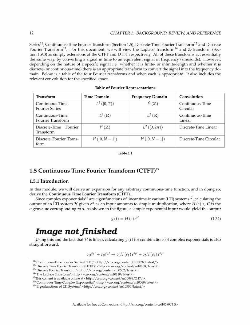
Series11, Continuous-Time Fourier Transform (Section 1.5), Discrete-Time Fourier Transform12 and DiscreteFourier Transform13. For this document, we will view the Laplace Transform14 and Z-Transform (Sec-tion 1.9.3) as simply extensions of the CTFT and DTFT respectively. All of these transforms act essentiallythe same way, by converting a signal in time to an equivalent signal in frequency (sinusoids). However,depending on the nature of a specific signal i.e. whether it is finite- or infinite-length and whether it isdiscrete- or continuous-time) there is an appropriate transform to convert the signal into the frequency do-main. Below is a table of the four Fourier transforms and when each is appropriate. It also includes therelevant convolution for the specified space.
Table of Fourier Representations
Transform Time Domain Frequency Domain Convolution
Continuous-TimeFourier Series
L2 ([0, T)) l2 (Z) Continuous-TimeCircular
Continuous-TimeFourier Transform
L2 (R) L2 (R) Continuous-TimeLinear
Discrete-Time FourierTransform
l2 (Z) L2 ([0, 2π)) Discrete-Time Linear
Discrete Fourier Trans-form
l2 ([0, N − 1]) l2 ([0, N − 1]) Discrete-Time Circular
Table 1.1
1.5 Continuous Time Fourier Transform (CTFT)15
1.5.1 Introduction
In this module, we will derive an expansion for any arbitrary continuous-time function, and in doing so,derive the Continuous Time Fourier Transform (CTFT).
Since complex exponentials16 are eigenfunctions of linear time-invariant (LTI) systems17, calculating theoutput of an LTI system H given est as an input amounts to simple multiplication, where H (s) ∈ C is theeigenvalue corresponding to s. As shown in the figure, a simple exponential input would yield the output
y (t) = H (s) est (1.34)
Using this and the fact thatH is linear, calculating y (t) for combinations of complex exponentials is alsostraightforward.
c1es1t + c2es2t → c1H (s1) es1t + c2H (s2) es2t
11"Continuous-Time Fourier Series (CTFS)" <http://cnx.org/content/m10097/latest/>12"Discrete Time Fourier Transform (DTFT)" <http://cnx.org/content/m10108/latest/>13"Discrete Fourier Transform" <http://cnx.org/content/m0502/latest/>14"The Laplace Transform" <http://cnx.org/content/m10110/latest/>15This content is available online at <http://cnx.org/content/m10098/2.17/>.16"Continuous Time Complex Exponential" <http://cnx.org/content/m10060/latest/>17"Eigenfunctions of LTI Systems" <http://cnx.org/content/m10500/latest/>
Available for free at Connexions <http://cnx.org/content/col10599/1.5>

13
∑n
cnesnt →∑n
cn H (sn) esnt
The action of H on an input such as those in the two equations above is easy to explain. H inde-pendently scales each exponential component esnt by a different complex number H (sn) ∈ C. As such, ifwe can write a function f (t) as a combination of complex exponentials it allows us to easily calculate theoutput of a system.
Now, we will look to use the power of complex exponentials to see how we may represent arbitrarysignals in terms of a set of simpler functions by superposition of a number of complex exponentials. Belowwe will present the Continuous-Time Fourier Transform (CTFT), commonly referred to as just the FourierTransform (FT). Because the CTFT deals with nonperiodic signals, we must find a way to include all realfrequencies in the general equations. For the CTFT we simply utilize integration over real numbers ratherthan summation over integers in order to express the aperiodic signals.
1.5.2 Fourier Transform Synthesis
Joseph Fourier18 demonstrated that an arbitrary s (t) can be written as a linear combination of harmoniccomplex sinusoids
s (t) =∞
∑n=−∞
cnejω0nt (1.35)
where ω0 = 2πT is the fundamental frequency. For almost all s (t) of practical interest, there exists cn to make
(1.35) true. If s (t) is finite energy ( s (t) ∈ L2 [0, T]), then the equality in (1.35) holds in the sense of energyconvergence; if s (t) is continuous, then (1.35) holds pointwise. Also, if s (t) meets some mild conditions(the Dirichlet conditions), then (1.35) holds pointwise everywhere except at points of discontinuity.
The cn - called the Fourier coefficients - tell us "how much" of the sinusoid ejω0nt is in s (t). The formulashows s (t) as a sum of complex exponentials, each of which is easily processed by an LTI system (since itis an eigenfunction of every LTI system). Mathematically, it tells us that the set of complex exponentials
ejω0nt , n ∈ Z
form a basis for the space of T-periodic continuous time functions.
1.5.2.1 Equations
Now, in order to take this useful tool and apply it to arbitrary non-periodic signals, we will have to delvedeeper into the use of the superposition principle. Let sT (t) be a periodic signal having period T. We wantto consider what happens to this signal’s spectrum as the period goes to infinity. We denote the spectrumfor any assumed value of the period by cn (T). We calculate the spectrum according to the Fourier formulafor a periodic signal, known as the Fourier Series (for more on this derivation, see the section on FourierSeries.)
cn =1T
∫ T
0s (t) exp (−ßω0t) dt (1.36)
where ω0 = 2πT and where we have used a symmetric placement of the integration interval about the origin
for subsequent derivational convenience. We vary the frequency index n proportionally as we increase theperiod. Define
ST ( f ) ≡ Tcn =1T
∫ T
0(ST ( f ) exp (ßω0t) dt(1.37)
making the corresponding Fourier Series
sT (t) =∞
∑−∞
f (t) exp (ßω0t)1T
(1.38)
18http://www-groups.dcs.st-and.ac.uk/∼history/Mathematicians/Fourier.html
Available for free at Connexions <http://cnx.org/content/col10599/1.5>

14 CHAPTER 1. BACKGROUND, REVIEW, AND REFERENCE
As the period increases, the spectral lines become closer together, becoming a continuum. Therefore,
limT→∞
sT (t) ≡ s (t) =∞∫−∞
S ( f ) exp (ßω0t) d f (1.39)
with
S ( f ) =∞∫−∞
s (t) exp (−ßω0t) dt (1.40)
Continuous-Time Fourier Transform
F (Ω) =∫ ∞
−∞f (t) e−(jΩt)dt (1.41)
Inverse CTFTf (t) =
12π
∫ ∞
−∞F (Ω) ejΩtdΩ (1.42)
WARNING: It is not uncommon to see the above formula written slightly different. One of the mostcommon differences is the way that the exponential is written. The above equations use the radialfrequency variable Ω in the exponential, where Ω = 2π f , but it is also common to include themore explicit expression, j2π f t, in the exponential. Click here19 for an overview of the notationused in Connexion’s DSP modules.
Example 1.2We know from Euler’s formula that cos (ωt) + sin (ωt) = 1−j
2 ejωt + 1+j2 e−jωt.
19"DSP notation" <http://cnx.org/content/m10161/latest/>
Available for free at Connexions <http://cnx.org/content/col10599/1.5>

15
1.5.3 CTFT Definition Demonstration
Figure 1.4: Interact (when online) with a Mathematica CDF demonstrating Continuous Time Fourier Trans-form. To Download, right-click and save as .cdf.
1.5.4 Example Problems
Exercise 1.5.1 (Solution on p. 71.)Find the Fourier Transform (CTFT) of the function
f (t) =
e−(αt) if t ≥ 0
0 otherwise(1.43)
Exercise 1.5.2 (Solution on p. 71.)Find the inverse Fourier transform of the ideal lowpass filter defined by
X (Ω) =
1 if |Ω| ≤ M
0 otherwise(1.44)
1.5.5 Fourier Transform Summary
Because complex exponentials are eigenfunctions of LTI systems, it is often useful to represent signals usinga set of complex exponentials as a basis. The continuous time Fourier series synthesis formula expresses a
Available for free at Connexions <http://cnx.org/content/col10599/1.5>

16 CHAPTER 1. BACKGROUND, REVIEW, AND REFERENCE
continuous time, periodic function as the sum of continuous time, discrete frequency complex exponentials.
f (t) =∞
∑n=−∞
cnejω0nt (1.45)
The continuous time Fourier series analysis formula gives the coefficients of the Fourier series expansion.
cn =1T
∫ T
0f (t) e−(jω0nt)dt (1.46)
In both of these equations ω0 = 2πT is the fundamental frequency.
1.6 Discrete-Time Fourier Transform (DTFT)20
The Fourier transform of the discrete-time signal s (n) is defined to be
S(
ej2π f)
=∞
∑n=−∞
s (n) e−(j2π f n) (1.47)
Frequency here has no units. As should be expected, this definition is linear, with the transform of a sumof signals equaling the sum of their transforms. Real-valued signals have conjugate-symmetric spectra:
S(
e−(j2π f ))
= S(
ej2π f)∗
.
Exercise 1.6.1 (Solution on p. 71.)A special property of the discrete-time Fourier transform is that it is periodic with period one:
S(
ej2π( f +1))
= S(
ej2π f)
. Derive this property from the definition of the DTFT.
Because of this periodicity, we need only plot the spectrum over one period to understand completely thespectrum’s structure; typically, we plot the spectrum over the frequency range
[− 1
2 , 12
]. When the signal
is real-valued, we can further simplify our plotting chores by showing the spectrum only over[0, 1
2
]; the
spectrum at negative frequencies can be derived from positive-frequency spectral values.When we obtain the discrete-time signal via sampling an analog signal, the Nyquist frequency21 corre-
sponds to the discrete-time frequency 12 . To show this, note that a sinusoid having a frequency equal to the
Nyquist frequency 12Ts
has a sampled waveform that equals
cos(
2π × 12Ts
nTs)
= cos (πn) = (−1)n
The exponential in the DTFT at frequency 12 equals e−
j2πn2 = e−(jπn) = (−1)n, meaning that discrete-time
frequency equals analog frequency multiplied by the sampling interval
fD = fATs (1.48)
fD and fA represent discrete-time and analog frequency variables, respectively. The aliasing figure22 pro-vides another way of deriving this result. As the duration of each pulse in the periodic sampling signalpTs (t) narrows, the amplitudes of the signal’s spectral repetitions, which are governed by the Fourier seriescoefficients23 of pTs (t), become increasingly equal. Examination of the periodic pulse signal24 reveals that
20This content is available online at <http://cnx.org/content/m10247/2.31/>.21"The Sampling Theorem" <http://cnx.org/content/m0050/latest/#para1>22"The Sampling Theorem", Figure 2: aliasing <http://cnx.org/content/m0050/latest/#alias>23"Complex Fourier Series", (10) <http://cnx.org/content/m0042/latest/#eqn2>24"Complex Fourier Series", Figure 1 <http://cnx.org/content/m0042/latest/#pps>
Available for free at Connexions <http://cnx.org/content/col10599/1.5>

17
as ∆ decreases, the value of c0, the largest Fourier coefficient, decreases to zero: |c0| = A∆Ts
. Thus, to maintaina mathematically viable Sampling Theorem, the amplitude A must increase as 1
∆ , becoming infinitely largeas the pulse duration decreases. Practical systems use a small value of ∆, say 0.1 · Ts and use amplifiers torescale the signal. Thus, the sampled signal’s spectrum becomes periodic with period 1
Ts. Thus, the Nyquist
frequency 12Ts
corresponds to the frequency 12 .
Example 1.3Let’s compute the discrete-time Fourier transform of the exponentially decaying sequence s (n) =anu (n), where u (n) is the unit-step sequence. Simply plugging the signal’s expression into theFourier transform formula,
S(
ej2π f)
= ∑∞n=−∞ anu (n) e−(j2π f n)
= ∑∞n=0
(ae−(j2π f )
)n (1.49)
This sum is a special case of the geometric series.
∞
∑n=0
αn =1
1− α, |α| < 1 (1.50)
Thus, as long as |a| < 1, we have our Fourier transform.
S(
ej2π f)
=1
1− ae−(j2π f )(1.51)
Using Euler’s relation, we can express the magnitude and phase of this spectrum.
|S(
ej2π f)| = 1√
(1− acos (2π f ))2 + a2sin2 (2π f )(1.52)
∠(
S(
ej2π f))
= −tan−1(
asin (2π f )1− acos (2π f )
)(1.53)
No matter what value of a we choose, the above formulae clearly demonstrate the periodic natureof the spectra of discrete-time signals. Figure 1.5 (Spectrum of exponential signal) shows indeedthat the spectrum is a periodic function. We need only consider the spectrum between − 1
2 and 12
to unambiguously define it. When a > 0, we have a lowpass spectrum—the spectrum diminishesas frequency increases from 0 to 1
2 —with increasing a leading to a greater low frequency content;for a < 0, we have a highpass spectrum (Figure 1.6 (Spectra of exponential signals)).
Available for free at Connexions <http://cnx.org/content/col10599/1.5>

18 CHAPTER 1. BACKGROUND, REVIEW, AND REFERENCE
Spectrum of exponential signal
-2 -1 0 1 2
1
2
f
|S(ej2πf)|
-2 -1 1 2
-45
45
f
∠S(ej2πf)
Figure 1.5: The spectrum of the exponential signal (a = 0.5) is shown over the frequency range [-2, 2],clearly demonstrating the periodicity of all discrete-time spectra. The angle has units of degrees.
Available for free at Connexions <http://cnx.org/content/col10599/1.5>

19
Spectra of exponential signals
f
a = 0.9
a = 0.5
a = –0.5
Spe
ctra
l Mag
nitu
de (
dB)
-10
0
10
20
0.5
a = 0.9
a = 0.5
a = –0.5
Ang
le (
degr
ees)
f
-90
-45
0
45
90
0.5
Figure 1.6: The spectra of several exponential signals are shown. What is the apparent relationshipbetween the spectra for a = 0.5 and a = −0.5?
Example 1.4Analogous to the analog pulse signal, let’s find the spectrum of the length-N pulse sequence.
s (n) =
1 if 0 ≤ n ≤ N − 1
0 otherwise(1.54)
The Fourier transform of this sequence has the form of a truncated geometric series.
S(
ej2π f)
=N−1
∑n=0
e−(j2π f n) (1.55)
For the so-called finite geometric series, we know that
N+n0−1
∑n=n0
αn = αn01− αN
1− α(1.56)
for all values of α.Exercise 1.6.2 (Solution on p. 71.)
Derive this formula for the finite geometric series sum. The "trick" is to consider the differencebetween the series’ sum and the sum of the series multiplied by α.
Applying this result yields (Figure 1.7 (Spectrum of length-ten pulse).)
S(
ej2π f)
= 1−e−(j2π f N)
1−e−(j2π f )
= e−(jπ f (N−1)) sin(π f N)sin(π f )
(1.57)
Available for free at Connexions <http://cnx.org/content/col10599/1.5>

20 CHAPTER 1. BACKGROUND, REVIEW, AND REFERENCE
The ratio of sine functions has the generic form of sin(Nx)sin(x) , which is known as the discrete-time sinc func-
tion dsinc (x). Thus, our transform can be concisely expressed as S(
ej2π f)
= e−(jπ f (N−1))dsinc (π f ). Thediscrete-time pulse’s spectrum contains many ripples, the number of which increase with N, the pulse’sduration.
Spectrum of length-ten pulse
Figure 1.7: The spectrum of a length-ten pulse is shown. Can you explain the rather complicated appear-ance of the phase?
The inverse discrete-time Fourier transform is easily derived from the following relationship:
∫ 12− 1
2e−(j2π f m)ej2π f nd f =
1 if m = n
0 if m 6= n
= δ (m− n)
(1.58)
Therefore, we find that∫ 12− 1
2S(
ej2π f)
ej2π f nd f =∫ 1
2− 1
2∑mm s (m) e−(j2π f m)ej2π f nd f
= ∑mm s (m)∫ 1
2− 1
2e(−(j2π f ))(m−n)d f
= s (n)
(1.59)
The Fourier transform pairs in discrete-time are
S(
ej2π f)
= ∑∞n=−∞ s (n) e−(j2π f n)
s (n) =∫ 1
2− 1
2S(
ej2π f)
ej2π f nd f(1.60)
Available for free at Connexions <http://cnx.org/content/col10599/1.5>

21
The properties of the discrete-time Fourier transform mirror those of the analog Fourier transform. TheDTFT properties table 25 shows similarities and differences. One important common property is Parseval’sTheorem.
∞
∑n=−∞
(|s (n) |)2 =∫ 1
2
− 12
(|S(
ej2π f)|)2
d f (1.61)
To show this important property, we simply substitute the Fourier transform expression into the frequency-domain expression for power.∫ 1
2− 1
2
(|S(
ej2π f)|)2
d f =∫ 1
2− 1
2∑nn s (n) e−(j2π f n) ∑mm s (n)∗ej2π f md f
= ∑n,mn,m s (n) s (n)∗∫ 1
2− 1
2ej2π f (m−n)d f
(1.62)
Using the orthogonality relation (1.58), the integral equals δ (m− n), where δ (n) is the unit sample (Fig-ure 1.2: Unit sample). Thus, the double sum collapses into a single sum because nonzero values occur onlywhen n = m, giving Parseval’s Theorem as a result. We term ∑nn s2 (n) the energy in the discrete-timesignal s (n) in spite of the fact that discrete-time signals don’t consume (or produce for that matter) energy.This terminology is a carry-over from the analog world.
Exercise 1.6.3 (Solution on p. 71.)Suppose we obtained our discrete-time signal from values of the product s (t) pTs (t), where the
duration of the component pulses in pTs (t) is ∆. How is the discrete-time signal energy related tothe total energy contained in s (t)? Assume the signal is bandlimited and that the sampling ratewas chosen appropriate to the Sampling Theorem’s conditions.
1.7 DFT as a Matrix Operation26
25"Properties of the DTFT" <http://cnx.org/content/m0506/latest/>26This content is available online at <http://cnx.org/content/m10962/2.5/>.
Available for free at Connexions <http://cnx.org/content/col10599/1.5>

22 CHAPTER 1. BACKGROUND, REVIEW, AND REFERENCE
1.7.1 Matrix Review
Recall:
• Vectors in RN :
x =
x0
x1
. . .
xN−1
, xi ∈ R
• Vectors in CN :
x =
x0
x1
. . .
xN−1
, xi ∈ C
• Transposition:
a. transpose:x
T=(
x0 x1 . . . xN−1
)b. conjugate:
x
H=(
x0∗ x1
∗ . . . xN−1∗)
• Inner product27:
a. real:x
T y =
N−1
∑i=0
xiyi
b. complex:x
H y =
N−1
∑i=0
xn∗yn
• Matrix Multiplication:
Ax =
a00 a01 . . . a0,N−1
a10 a11 . . . a1,N−1...
... . . ....
aN−1,0 aN−1,1 . . . aN−1,N−1
x0
x1
. . .
xN−1
=
y0
y1
. . .
yN−1
yk =
N−1
∑n=0
aknxn
• Matrix Transposition:
AT =
a00 a10 . . . aN−1,0
a01 a11 . . . aN−1,1...
... . . ....
a0,N−1 a1,N−1 . . . aN−1,N−1
27"Inner Products" <http://cnx.org/content/m10755/latest/>
Available for free at Connexions <http://cnx.org/content/col10599/1.5>

23
Matrix transposition involved simply swapping the rows with columns.
AH = AT∗
The above equation is Hermitian transpose.
A
Tk,n =
An,k
AHk,n =
A∗
n,k
1.7.2 Representing DFT as Matrix Operation
Now let’s represent the DFT28 in vector-matrix notation.
x =
x [0]
x [1]
. . .
x [N − 1]
X=
X [0]
X [1]
. . .
X [N − 1]
∈ CN
Herex is the vector of time samples and
X is the vector of DFT coefficients. How are
x and
X related:
X [k] =N−1
∑n=0
x [n] e−(j 2πN kn)
whereakn =
(e−(j 2π
N ))kn
= WNkn
soX= W
x
whereX is the DFT vector, W is the matrix and
x the time domain vector.
Wk,n =(
e−(j 2πN ))kn
X= W
x [0]
x [1]
. . .
x [N − 1]
28"Discrete Fourier Transform (DFT)" <http://cnx.org/content/m10249/latest/>
Available for free at Connexions <http://cnx.org/content/col10599/1.5>

24 CHAPTER 1. BACKGROUND, REVIEW, AND REFERENCE
IDFT:
x [n] =1N
N−1
∑k=0
X [k](
ej 2πN
)nk
where (ej 2π
N
)nk= WN
nk∗
WNnk∗ is the matrix Hermitian transpose. So,
x =
1N
WH X
wherex is the time vector, 1
N WH is the inverse DFT matrix, andX is the DFT vector.
1.8 Sampling theory
1.8.1 Introduction29
Contents of Sampling chapter
• Introduction(Current module)• Proof (Section 1.8.2)• Illustrations (Section 1.8.3)• Matlab Example30
• Hold operation31
• System view (Section 1.8.4)• Aliasing applet32
• Exercises33
• Table of formulas34
1.8.1.1 Why sample?
This section introduces sampling. Sampling is the necessary fundament for all digital signal processing andcommunication. Sampling can be defined as the process of measuring an analog signal at distinct points.
Digital representation of analog signals offers advantages in terms of
• robustness towards noise, meaning we can send more bits/s• use of flexible processing equipment, in particular the computer• more reliable processing equipment• easier to adapt complex algorithms
29This content is available online at <http://cnx.org/content/m11419/1.29/>.30"Sampling and reconstruction with Matlab" <http://cnx.org/content/m11549/latest/>31"Hold operation" <http://cnx.org/content/m11458/latest/>32"Aliasing Applet" <http://cnx.org/content/m11448/latest/>33"Exercises" <http://cnx.org/content/m11442/latest/>34"Table of Formulas" <http://cnx.org/content/m11450/latest/>
Available for free at Connexions <http://cnx.org/content/col10599/1.5>

25
1.8.1.2 Claude E. Shannon
Figure 1.8: Claude Elwood Shannon (1916-2001)
Claude Shannon35 has been called the father of information theory, mainly due to his landmark paperson the "Mathematical theory of communication"36 . Harry Nyquist37 was the first to state the samplingtheorem in 1928, but it was not proven until Shannon proved it 21 years later in the paper "Communicationsin the presence of noise"38 .
1.8.1.3 Notation
In this chapter we will be using the following notation
• Original analog signal x (t)• Sampling frequency Fs• Sampling interval Ts (Note that: Fs = 1
Ts)
• Sampled signal xs (n). (Note that xs (n) = x (nTs))• Real angular frequency Ω• Digital angular frequency ω. (Note that: ω = ΩTs)
1.8.1.4 The Sampling Theorem
NOTE: When sampling an analog signal the sampling frequency must be greater than twice thehighest frequency component of the analog signal to be able to reconstruct the original signal fromthe sampled version.
35http://www.research.att.com/∼njas/doc/ces5.html36http://cm.bell-labs.com/cm/ms/what/shannonday/shannon1948.pdf37http://www.wikipedia.org/wiki/Harry_Nyquist38http://www.stanford.edu/class/ee104/shannonpaper.pdf
Available for free at Connexions <http://cnx.org/content/col10599/1.5>

26 CHAPTER 1. BACKGROUND, REVIEW, AND REFERENCE
1.8.1.5
Finished? Have at look at: Proof (Section 1.8.2); Illustrations (Section 1.8.3); Matlab Example39; Aliasingapplet40; Hold operation41; System view (Section 1.8.4); Exercises42
1.8.2 Proof43
NOTE: In order to recover the signal x (t) from it’s samples exactly, it is necessary to sample x (t)at a rate greater than twice it’s highest frequency component.
1.8.2.1 Introduction
As mentioned earlier (p. 24), sampling is the necessary fundament when we want to apply digital signalprocessing on analog signals.
Here we present the proof of the sampling theorem. The proof is divided in two. First we find anexpression for the spectrum of the signal resulting from sampling the original signal x (t). Next we showthat the signal x (t) can be recovered from the samples. Often it is easier using the frequency domain whencarrying out a proof, and this is also the case here.Key points in the proof
• We find an equation (1.70) for the spectrum of the sampled signal• We find a simple method to reconstruct (1.76) the original signal• The sampled signal has a periodic spectrum...• ...and the period is 2× πFs
1.8.2.2 Proof part 1 - Spectral considerations
By sampling x (t) every Ts second we obtain xs (n). The inverse fourier transform of this time discretesignal44 is
xs (n) =1
2π
∫ π
−πXs
(ejω)
ejωndω (1.63)
For convenience we express the equation in terms of the real angular frequency Ω using ω = ΩTs. We thenobtain
xs (n) =Ts
2π
∫ πTs
−πTs
Xs
(ejΩTs
)ejΩTsndΩ (1.64)
The inverse fourier transform of a continuous signal is
x (t) =1
2π
∫ ∞
−∞X (jΩ) ejΩtdΩ (1.65)
From this equation we find an expression for x (nTs)
x (nTs) =1
2π
∫ ∞
−∞X (jΩ) ejΩnTs dΩ (1.66)
39"Sampling and reconstruction with Matlab" <http://cnx.org/content/m11549/latest/>40"Aliasing Applet" <http://cnx.org/content/m11448/latest/>41"Hold operation" <http://cnx.org/content/m11458/latest/>42"Exercises" <http://cnx.org/content/m11442/latest/>43This content is available online at <http://cnx.org/content/m11423/1.27/>.44"Discrete time signals" <http://cnx.org/content/m11476/latest/>
Available for free at Connexions <http://cnx.org/content/col10599/1.5>

27
To account for the difference in region of integration we split the integration in (1.66) into subintervals oflength 2π
Tsand then take the sum over the resulting integrals to obtain the complete area.
x (nTs) =1
2π
∞
∑k=−∞
∫ (2k+1)πTs
(2k−1)πTs
X (jΩ) ejΩnTs dΩ (1.67)
Then we change the integration variable, setting Ω = η + 2×πkTs
x (nTs) =1
2π
∞
∑k=−∞
∫ πTs
−πTs
X(
j(
η +2× πk
Ts
))ej(η+ 2×πk
Ts )nTs dη (1.68)
We obtain the final form by observing that ej2×πkn = 1, reinserting η = Ω and multiplying by TsTs
x (nTs) =Ts
2π
∫ πTs
−πTs
∞
∑k=−∞
1Ts
X(
j(
Ω +2× πk
Ts
))ejΩnTs dΩ (1.69)
To make xs (n) = x (nTs) for all values of n, the integrands in (1.64) and (1.69) have to agreee, that is
Xs
(ejΩTs
)=
1Ts
∞
∑k=−∞
X(
j(
Ω +2πkTs
))(1.70)
This is a central result. We see that the digital spectrum consists of a sum of shifted versions of the original,analog spectrum. Observe the periodicity!
We can also express this relation in terms of the digital angular frequency ω = ΩTs
Xs
(ejω)
=1Ts
∞
∑k=−∞
X(
jω + 2× πk
Ts
)(1.71)
This concludes the first part of the proof. Now we want to find a reconstruction formula, so that we canrecover x (t) from xs (n).
1.8.2.3 Proof part II - Signal reconstruction
For a bandlimited (Figure 1.10) signal the inverse fourier transform is
x (t) =1
2π
∫ πTs
−πTs
X (jΩ) ejΩtdΩ (1.72)
In the interval we are integrating we have: Xs(ejΩTs
)= X(jΩ)
Ts. Substituting this relation into (1.72) we get
x (t) =Ts
2π
∫ πTs
−πTs
Xs
(ejΩTs
)ejΩtdΩ (1.73)
Using the DTFT45 relation for Xs(ejΩTs
)we have
x (t) =Ts
2π
∫ πTs
−πTs
∞
∑n=−∞
xs (n) e−(jΩnTs)ejΩtdΩ (1.74)
Interchanging integration and summation (under the assumption of convergence) leads to
x (t) =Ts
2π
∞
∑n=−∞
xs (n)∫ π
Ts
−πTs
ejΩ(t−nTs)dΩ (1.75)
45"Table of Formulas" <http://cnx.org/content/m11450/latest/>
Available for free at Connexions <http://cnx.org/content/col10599/1.5>

28 CHAPTER 1. BACKGROUND, REVIEW, AND REFERENCE
Finally we perform the integration and arrive at the important reconstruction formula
x (t) =∞
∑n=−∞
xs (n)sin(
πTs
(t− nTs))
πTs
(t− nTs)(1.76)
(Thanks to R.Loos for pointing out an error in the proof.)
Available for free at Connexions <http://cnx.org/content/col10599/1.5>

29
1.8.2.4 Summary
NOTE: Xs(ejΩTs
)= 1
Ts∑∞
k=−∞ X(
j(
Ω + 2πkTs
))
NOTE: x (t) = ∑∞n=−∞ xs (n)
sin( πTs (t−nTs))
πTs (t−nTs)
1.8.2.5
Go to Introduction (Section 1.8.1); Illustrations (Section 1.8.3); Matlab Example46; Hold operation47; Alias-ing applet48; System view (Section 1.8.4); Exercises49 ?
1.8.3 Illustrations50
In this module we illustrate the processes involved in sampling and reconstruction. To see how all theseprocesses work together as a whole, take a look at the system view (Section 1.8.4). In Sampling and recon-struction with Matlab51 we provide a Matlab script for download. The matlab script shows the process ofsampling and reconstruction live.
1.8.3.1 Basic examples
Example 1.5To sample an analog signal with 3000 Hz as the highest frequency component requires sampling
at 6000 Hz or above.
Example 1.6The sampling theorem can also be applied in two dimensions, i.e. for image analysis. A 2D
sampling theorem has a simple physical interpretation in image analysis: Choose the samplinginterval such that it is less than or equal to half of the smallest interesting detail in the image.
1.8.3.2 The process of sampling
We start off with an analog signal. This can for example be the sound coming from your stereo at home oryour friend talking.
The signal is then sampled uniformly. Uniform sampling implies that we sample every Ts seconds. InFigure 1.9 we see an analog signal. The analog signal has been sampled at times t = nTs.
46"Sampling and reconstruction with Matlab" <http://cnx.org/content/m11549/latest/>47"Hold operation" <http://cnx.org/content/m11458/latest/>48"Aliasing Applet" <http://cnx.org/content/m11448/latest/>49"Exercises" <http://cnx.org/content/m11442/latest/>50This content is available online at <http://cnx.org/content/m11443/1.33/>.51"Sampling and reconstruction with Matlab" <http://cnx.org/content/m11549/latest/>
Available for free at Connexions <http://cnx.org/content/col10599/1.5>

30 CHAPTER 1. BACKGROUND, REVIEW, AND REFERENCE
Figure 1.9: Analog signal, samples are marked with dots.
In signal processing it is often more convenient and easier to work in the frequency domain. So let’s lookat at the signal in frequency domain, Figure 1.10. For illustration purposes we take the frequency contentof the signal as a triangle. (If you Fourier transform the signal in Figure 1.9 you will not get such a nicetriangle.)
Figure 1.10: The spectrum X (jΩ).
Notice that the signal in Figure 1.10 is bandlimited. We can see that the signal is bandlimited because
Available for free at Connexions <http://cnx.org/content/col10599/1.5>

31
X (jΩ) is zero outside the interval[−Ωg, Ωg
]. Equivalentely we can state that the signal has no angular
frequencies above Ωg, corresponding to no frequencies above Fg = Ωg2π .
Now let’s take a look at the sampled signal in the frequency domain. While proving (Section 1.8.2) thesampling theorem we found the the spectrum of the sampled signal consists of a sum of shifted versions ofthe analog spectrum. Mathematically this is described by the following equation:
Xs
(ejΩTs
)=
1Ts
∞
∑k=−∞
X(
j(
Ω +2πkTs
))(1.77)
1.8.3.2.1 Sampling fast enough
In Figure 1.11 we show the result of sampling x (t) according to the sampling theorem (Section 1.8.1.4: TheSampling Theorem). This means that when sampling the signal in Figure 1.9/Figure 1.10 we use Fs ≥ 2Fg.Observe in Figure 1.11 that we have the same spectrum as in Figure 1.10 for Ω ∈
[−Ωg, Ωg
], except for the
scaling factor 1Ts
. This is a consequence of the sampling frequency. As mentioned in the proof (Key pointsin the proof, p. 26) the spectrum of the sampled signal is periodic with period 2πFs = 2π
Ts.
Figure 1.11: The spectrum Xs. Sampling frequency is OK.
So now we are, according to the sample theorem (Section 1.8.1.4: The Sampling Theorem), able to recon-struct the original signal exactly. How we can do this will be explored further down under reconstruction(Section 1.8.3.3: Reconstruction). But first we will take a look at what happens when we sample too slowly.
1.8.3.2.2 Sampling too slowly
If we sample x (t) too slowly, that is Fs < 2Fg, we will get overlap between the repeated spectra, seeFigure 1.12. According to (1.77) the resulting spectra is the sum of these. This overlap gives rise to theconcept of aliasing.
NOTE: If the sampling frequency is less than twice the highest frequency component, then fre-quencies in the original signal that are above half the sampling rate will be "aliased" and willappear in the resulting signal as lower frequencies.
The consequence of aliasing is that we cannot recover the original signal, so aliasing has to be avoided.Sampling too slowly will produce a sequence xs (n) that could have orginated from a number of signals.So there is no chance of recovering the original signal. To learn more about aliasing, take a look at thismodule52. (Includes an applet for demonstration!)
52"Aliasing Applet" <http://cnx.org/content/m11448/latest/>
Available for free at Connexions <http://cnx.org/content/col10599/1.5>

32 CHAPTER 1. BACKGROUND, REVIEW, AND REFERENCE
Figure 1.12: The spectrum Xs. Sampling frequency is too low.
To avoid aliasing we have to sample fast enough. But if we can’t sample fast enough (possibly due tocosts) we can include an Anti-Aliasing filter. This will not able us to get an exact reconstruction but can stillbe a good solution.
NOTE: Typically a low-pass filter that is applied before sampling to ensure that no componentswith frequencies greater than half the sample frequency remain.
Example 1.7The stagecoach effect
In older western movies you can observe aliasing on a stagecoach when it starts to roll. At firstthe spokes appear to turn forward, but as the stagecoach increase its speed the spokes appear toturn backward. This comes from the fact that the sampling rate, here the number of frames persecond, is too low. We can view each frame as a sample of an image that is changing continuouslyin time. (Applet illustrating the stagecoach effect53 )
1.8.3.3 Reconstruction
Given the signal in Figure 1.11 we want to recover the original signal, but the question is how?When there is no overlapping in the spectrum, the spectral component given by k = 0 (see (1.77)),is
equal to the spectrum of the analog signal. This offers an oppurtunity to use a simple reconstruction process.Remember what you have learned about filtering. What we want is to change signal in Figure 1.11 into thatof Figure 1.10. To achieve this we have to remove all the extra components generated in the samplingprocess. To remove the extra components we apply an ideal analog low-pass filter as shown in Figure 1.13As we see the ideal filter is rectangular in the frequency domain. A rectangle in the frequency domaincorresponds to a sinc54 function in time domain (and vice versa).
53http://flowers.ofthenight.org/wagonWheel/wagonWheel.html54http://ccrma-www.stanford.edu/∼jos/Interpolation/sinc_function.html
Available for free at Connexions <http://cnx.org/content/col10599/1.5>

33
Figure 1.13: H (jΩ) The ideal reconstruction filter.
Then we have reconstructed the original spectrum, and as we know if two signals are identical in thefrequency domain, they are also identical in the time domain. End of reconstruction.
1.8.3.4 Conclusions
The Shannon sampling theorem requires that the input signal prior to sampling is band-limited to at mosthalf the sampling frequency. Under this condition the samples give an exact signal representation. It istruly remarkable that such a broad and useful class signals can be represented that easily!
We also looked into the problem of reconstructing the signals form its samples. Again the simplicity ofthe principle is striking: linear filtering by an ideal low-pass filter will do the job. However, the ideal filteris impossible to create, but that is another story...
1.8.3.5
Go to? Introduction (Section 1.8.1); Proof (Section 1.8.2); Illustrations (Section 1.8.3); Matlab Example55;Aliasing applet56; Hold operation57; System view (Section 1.8.4); Exercises58
1.8.4 Systems view of sampling and reconstruction59
1.8.4.1 Ideal reconstruction system
Figure 1.14 shows the ideal reconstruction system based on the results of the Sampling theorem proof(Section 1.8.2).
Figure 1.14 consists of a sampling device which produces a time-discrete sequence xs (n). The recon-struction filter, h (t), is an ideal analog sinc60 filter, with h (t) = sinc
(t
Ts
). We can’t apply the time-discrete
sequence xs (n) directly to the analog filter h (t). To solve this problem we turn the sequence into an analogsignal using delta functions61. Thus we write xs (t) = ∑∞
n=−∞ xs (n) δ (t− nT).
55"Sampling and reconstruction with Matlab" <http://cnx.org/content/m11549/latest/>56"Aliasing Applet" <http://cnx.org/content/m11448/latest/>57"Hold operation" <http://cnx.org/content/m11458/latest/>58"Exercises" <http://cnx.org/content/m11442/latest/>59This content is available online at <http://cnx.org/content/m11465/1.20/>.60http://ccrma-www.stanford.edu/∼jos/Interpolation/sinc_function.html61"Table of Formulas" <http://cnx.org/content/m11450/latest/>
Available for free at Connexions <http://cnx.org/content/col10599/1.5>

34 CHAPTER 1. BACKGROUND, REVIEW, AND REFERENCE
Figure 1.14: Ideal reconstruction system
But when will the system produce an output x (t) = x (t)? According to the sampling theorem (Sec-tion 1.8.1.4: The Sampling Theorem) we have x (t) = x (t) when the sampling frequency, Fs, is at least twicethe highest frequency component of x (t).
1.8.4.2 Ideal system including anti-aliasing
To be sure that the reconstructed signal is free of aliasing it is customary to apply a lowpass filter, an anti-aliasing filter (p. 32), before sampling as shown in Figure 1.15.
Figure 1.15: Ideal reconstruction system with anti-aliasing filter (p. 32)
Again we ask the question of when the system will produce an output x (t) = s (t)? If the signal isentirely confined within the passband of the lowpass filter we will get perfect reconstruction if Fs is highenough.
But if the anti-aliasing filter removes the "higher" frequencies, (which in fact is the job of the anti-aliasingfilter), we will never be able to exactly reconstruct the original signal, s (t). If we sample fast enough wecan reconstruct x (t), which in most cases is satisfying.
The reconstructed signal, x (t), will not have aliased frequencies. This is essential for further use of thesignal.
1.8.4.3 Reconstruction with hold operation
To make our reconstruction system realizable there are many things to look into. Among them are the factthat any practical reconstruction system must input finite length pulses into the reconstruction filter. Thiscan be accomplished by the hold operation62. To alleviate the distortion caused by the hold opeator weapply the output from the hold device to a compensator. The compensation can be as accurate as we wish,this is cost and application consideration.
62"Hold operation" <http://cnx.org/content/m11458/latest/>
Available for free at Connexions <http://cnx.org/content/col10599/1.5>

35
Figure 1.16: More practical reconstruction system with a hold component63
By the use of the hold component the reconstruction will not be exact, but as mentioned above we canget as close as we want.
1.8.4.4
Introduction (Section 1.8.1); Proof (Section 1.8.2); Illustrations (Section 1.8.3); Matlab example64; Hold oper-ation65; Aliasing applet66; Exercises67
1.8.5 Sampling CT Signals: A Frequency Domain Perspective68
1.8.5.1 Understanding Sampling in the Frequency Domain
We want to relate xc (t) directly to x [n]. Compute the CTFT of
xs (t) =∞
∑n=−∞
xc (nT) δ (t− nT)
Xs (Ω) =∫ ∞−∞ ∑∞
n=−∞ xc (nT) δ (t− nT) e(−j)Ωtdt
= ∑∞n=−∞ xc (nT)
∫ ∞−∞ δ (t− nT) e(−j)Ωtdt
= ∑∞n=−∞ x [n] e(−j)ΩnT
= ∑∞n=−∞ x [n] e(−j)ωn
= X (ω)
(1.78)
where ω ≡ ΩT and X (ω) is the DTFT of x [n].
NOTE:
Xs (Ω) =1T
∞
∑k=−∞
Xc (Ω− kΩs)
X (ω) = 1T ∑∞
k=−∞ Xc (Ω− kΩs)
= 1T ∑∞
k=−∞ Xc
(ω−2πk
T
) (1.79)
where this last part is 2π-periodic.
63"Hold operation" <http://cnx.org/content/m11458/latest/>64"Sampling and reconstruction with Matlab" <http://cnx.org/content/m11549/latest/>65"Hold operation" <http://cnx.org/content/m11458/latest/>66"Aliasing Applet" <http://cnx.org/content/m11448/latest/>67"Exercises" <http://cnx.org/content/m11442/latest/>68This content is available online at <http://cnx.org/content/m10994/2.2/>.
Available for free at Connexions <http://cnx.org/content/col10599/1.5>

36 CHAPTER 1. BACKGROUND, REVIEW, AND REFERENCE
1.8.5.1.1 Sampling
Figure 1.17
Example 1.8: SpeechSpeech is intelligible if bandlimited by a CT lowpass filter to the band ±4 kHz. We can sample
speech as slowly as _____?
Available for free at Connexions <http://cnx.org/content/col10599/1.5>

37
Figure 1.18
Figure 1.19: Note that there is no mention of T or Ωs!
1.8.5.2 Relating x[n] to sampled x(t)
Recall the following equality:
xs (t) = ∑nn
x (nT) δ (t− nT)
Available for free at Connexions <http://cnx.org/content/col10599/1.5>

38 CHAPTER 1. BACKGROUND, REVIEW, AND REFERENCE
Figure 1.20
Recall the CTFT relation:
x (αt)↔ 1α
X(
Ωα
)(1.80)
where α is a scaling of time and 1α is a scaling in frequency.
Xs (Ω) ≡ X (ΩT) (1.81)
1.8.6 The DFT: Frequency Domain with a Computer Analysis69
1.8.6.1 Introduction
We just covered ideal (and non-ideal) (time) sampling of CT signals (Section 1.8.5). This enabled DT signalprocessing solutions for CT applications (Figure 1.21):
69This content is available online at <http://cnx.org/content/m10992/2.3/>.
Available for free at Connexions <http://cnx.org/content/col10599/1.5>

39
Figure 1.21
Much of the theoretical analysis of such systems relied on frequency domain representations. How dowe carry out these frequency domain analysis on the computer? Recall the following relationships:
x [n] DTFT↔ X (ω)
x (t) CTFT↔ X (Ω)
where ω and Ω are continuous frequency variables.
1.8.6.1.1 Sampling DTFT
Consider the DTFT of a discrete-time (DT) signal x [n]. Assume x [n] is of finite duration N (i.e., an N-pointsignal).
X (ω) =N−1
∑n=0
x [n] e(−j)ωn (1.82)
where X (ω) is the continuous function that is indexed by the real-valued parameter −π ≤ ω ≤ π. Theother function, x [n], is a discrete function that is indexed by integers.
We want to work with X (ω) on a computer. Why not just sample X (ω)?
X [k] = X( 2π
N k)
= ∑N−1n=0 x [n] e(−j)2π k
N n(1.83)
In (1.83) we sampled at ω = 2πN k where k = 0, 1, . . . , N − 1 and X [k] for k = 0, . . . , N − 1 is called the
Discrete Fourier Transform (DFT) of x [n].
Example 1.9
Finite Duration DT Signal
Figure 1.22
The DTFT of the image in Figure 1.22 (Finite Duration DT Signal) is written as follows:
X (ω) =N−1
∑n=0
x [n] e(−j)ωn (1.84)
Available for free at Connexions <http://cnx.org/content/col10599/1.5>

40 CHAPTER 1. BACKGROUND, REVIEW, AND REFERENCE
where ω is any 2π-interval, for example −π ≤ ω ≤ π.
Sample X(ω)
Figure 1.23
where again we sampled at ω = 2πN k where k = 0, 1, . . . , M− 1. For example, we take
M = 10
. In the following section (Section 1.8.6.1.1.1: Choosing M) we will discuss in more detail how weshould choose M, the number of samples in the 2π interval.
(This is precisely how we would plot X (ω) in Matlab.)
1.8.6.1.1.1 Choosing M
1.8.6.1.1.1.1 Case 1
Given N (length of x [n]), choose M N to obtain a dense sampling of the DTFT (Figure 1.24):
Figure 1.24
1.8.6.1.1.1.2 Case 2
Choose M as small as possible (to minimize the amount of computation).In general, we require M ≥ N in order to represent all information in
x [n] , n = 0, . . . , N − 1Let’s concentrate on M = N:
x [n] DFT↔ X [k]for n = 0, . . . , N − 1 and k = 0, . . . , N − 1
numbers↔ N numbers
Available for free at Connexions <http://cnx.org/content/col10599/1.5>

41
1.8.6.2 Discrete Fourier Transform (DFT)
Define
X [k] ≡ X(
2πkN
)(1.85)
where N = length (x [n]) and k = 0, . . . , N − 1. In this case, M = N.DFT
X [k] =N−1
∑n=0
x [n] e(−j)2π kN n (1.86)
Inverse DFT (IDFT)
x [n] =1N
N−1
∑k=0
X [k] ej2π kN n (1.87)
1.8.6.2.1 Interpretation
Represent x [n] in terms of a sum of N complex sinusoids70 of amplitudes X [k] and frequencies
ωk =2πkN
, k ∈ 0, . . . , N − 1
NOTE: Fourier Series with fundamental frequency 2πN
1.8.6.2.1.1 Remark 1
IDFT treats x [n] as though it were N-periodic.
x [n] =1N
N−1
∑k=0
X [k] ej2π kN n (1.88)
where n ∈ 0, . . . , N − 1Exercise 1.8.6.1 (Solution on p. 71.)What about other values of n?
1.8.6.2.1.2 Remark 2
Proof that the IDFT inverts the DFT for n ∈ 0, . . . , N − 1
1N ∑N−1
k=0 X [k] ej2π kN n = 1
N ∑N−1k=0 ∑N−1
m=0 x [m] e(−j)2π kN mej2π k
N n
= ???(1.89)
Example 1.10: Computing DFTGiven the following discrete-time signal (Figure 1.25) with N = 4, we will compute the DFT usingtwo different methods (the DFT Formula and Sample DTFT):
70"Continuous Time Complex Exponential" <http://cnx.org/content/m10060/latest/>
Available for free at Connexions <http://cnx.org/content/col10599/1.5>

42 CHAPTER 1. BACKGROUND, REVIEW, AND REFERENCE
Figure 1.25
1. DFT FormulaX [k] = ∑N−1
n=0 x [n] e(−j)2π kN n
= 1 + e(−j)2π k4 + e(−j)2π k
4 2 + e(−j)2π k4 3
= 1 + e(−j) π2 k + e(−j)πk + e(−j) 3
2 πk
(1.90)
Using the above equation, we can solve and get the following results:
x [0] = 4
x [1] = 0
x [2] = 0
x [3] = 0
2. Sample DTFT. Using the same figure, Figure 1.25, we will take the DTFT of the signal andget the following equations:
X (ω) = ∑3n=0 e(−j)ωn
= 1−e(−j)4ω
1−e(−j)ω
= ???
(1.91)
Our sample points will be:
ωk =2πk
4=
π
2k
where k = 0, 1, 2, 3 (Figure 1.26).
Available for free at Connexions <http://cnx.org/content/col10599/1.5>

43
Figure 1.26
1.8.6.3 Periodicity of the DFT
DFT X [k] consists of samples of DTFT, so X (ω), a 2π-periodic DTFT signal, can be converted to X [k], anN-periodic DFT.
X [k] =N−1
∑n=0
x [n] e(−j)2π kN n (1.92)
where e(−j)2π kN n is an N-periodic basis function (See Figure 1.27).
Figure 1.27
Also, recall,x [n] = 1
N ∑N−1n=0 X [k] ej2π k
N n
= 1N ∑N−1
n=0 X [k] ej2π kN (n+mN)
= ???
(1.93)
Available for free at Connexions <http://cnx.org/content/col10599/1.5>

44 CHAPTER 1. BACKGROUND, REVIEW, AND REFERENCE
Example 1.11: Illustration
Figure 1.28
NOTE: When we deal with the DFT, we need to remember that, in effect, this treats the signal asan N-periodic sequence.
1.8.6.4 A Sampling Perspective
Think of sampling the continuous function X (ω), as depicted in Figure 1.29. S (ω) will represent thesampling function applied to X (ω) and is illustrated in Figure 1.29 as well. This will result in our discrete-time sequence, X [k].
Available for free at Connexions <http://cnx.org/content/col10599/1.5>

45
Figure 1.29
NOTE: Remember the multiplication in the frequency domain is equal to convolution in the timedomain!
1.8.6.4.1 Inverse DTFT of S(ω)
∞
∑k=−∞
δ
(ω− 2πk
N
)(1.94)
Given the above equation, we can take the DTFT and get the following equation:
N∞
∑m=−∞
δ [n−mN] ≡ S [n] (1.95)
Exercise 1.8.6.2 (Solution on p. 71.)Why does (1.95) equal S [n]?
Available for free at Connexions <http://cnx.org/content/col10599/1.5>

46 CHAPTER 1. BACKGROUND, REVIEW, AND REFERENCE
So, in the time-domain we have (Figure 1.30):
Figure 1.30
Available for free at Connexions <http://cnx.org/content/col10599/1.5>

47
1.8.6.5 Connections
Figure 1.31
Combine signals in Figure 1.31 to get signals in Figure 1.32.
Figure 1.32
Available for free at Connexions <http://cnx.org/content/col10599/1.5>

48 CHAPTER 1. BACKGROUND, REVIEW, AND REFERENCE
1.8.7 Discrete-Time Processing of CT Signals71
1.8.7.1 DT Processing of CT Signals
DSP System
Figure 1.33
1.8.7.1.1 Analysis
Yc (Ω) = HLP (Ω) Y (ΩT) (1.96)
where we know that Y (ω) = X (ω) G (ω) and G (ω) is the frequency response of the DT LTI system. Also,remember that
ω ≡ ΩT
So,Yc (Ω) = HLP (Ω) G (ΩT) X (ΩT) (1.97)
where Yc (Ω) and HLP (Ω) are CTFTs and G (ΩT) and X (ΩT) are DTFTs.
NOTE:
X (ω) =2π
T
∞
∑k=−∞
Xc
(ω− 2πk
T
)OR
X (ΩT) =2π
T
∞
∑k=−∞
Xc (Ω− kΩs)
Therefore our final output signal, Yc (Ω), will be:
Yc (Ω) = HLP (Ω) G (ΩT)
(2π
T
∞
∑k=−∞
Xc (Ω− kΩs)
)(1.98)
71This content is available online at <http://cnx.org/content/m10993/2.2/>.
Available for free at Connexions <http://cnx.org/content/col10599/1.5>

49
Now, if Xc (Ω) is bandlimited to[−Ωs
2 , Ωs2
]and we use the usual lowpass reconstruction filter in the D/A,
Figure 1.34:
Figure 1.34
Then,
Yc (Ω) =
G (ΩT) Xc (Ω) if |Ω| < Ωs2
0 otherwise(1.99)
Available for free at Connexions <http://cnx.org/content/col10599/1.5>

50 CHAPTER 1. BACKGROUND, REVIEW, AND REFERENCE
1.8.7.1.2 Summary
For bandlimited signals sampled at or above the Nyquist rate, we can relate the input and output of theDSP system by:
Yc (Ω) = Ge f f (Ω) Xc (Ω) (1.100)
where
Ge f f (Ω) =
G (ΩT) if |Ω| < Ωs2
0 otherwise
Figure 1.35
1.8.7.1.2.1 Note
Ge f f (Ω) is LTI if and only if the following two conditions are satisfied:
1. G (ω) is LTI (in DT).2. Xc (T) is bandlimited and sampling rate equal to or greater than Nyquist. For example, if we had a
simple pulse described byXc (t) = u (t− T0)− u (t− T1)
where T1 > T0. If the sampling period T > T1 − T0, then some samples might "miss" the pulse whileothers might not be "missed." This is what we term time-varying behavior.
Example 1.12
Available for free at Connexions <http://cnx.org/content/col10599/1.5>

51
Figure 1.36
If 2πT > 2B and ω1 < BT, determine and sketch Yc (Ω) using Figure 1.36.
1.8.7.2 Application: 60Hz Noise Removal
Figure 1.37
Unfortunately, in real-world situations electrodes also pick up ambient 60 Hz signals from lights, comput-ers, etc.. In fact, usually this "60 Hz noise" is much greater in amplitude than the EKG signal shown inFigure 1.37. Figure 1.38 shows the EKG signal; it is barely noticeable as it has become overwhelmed bynoise.
Available for free at Connexions <http://cnx.org/content/col10599/1.5>

52 CHAPTER 1. BACKGROUND, REVIEW, AND REFERENCE
Figure 1.38: Our EKG signal, y (t), is overwhelmed by noise.
1.8.7.2.1 DSP Solution
Figure 1.39
Figure 1.40
1.8.7.2.2 Sampling Period/Rate
First we must note that |Y (Ω) | is bandlimited to ±60 Hz. Therefore, the minimum rate should be 120 Hz.In order to get the best results we should set
fs = 240Hz
Available for free at Connexions <http://cnx.org/content/col10599/1.5>

53
.
Ωs = 2π ×(
240rad
s
)
Figure 1.41
1.8.7.2.3 Digital Filter
Therefore, we want to design a digital filter that will remove the 60Hz component and preserve the rest.
Figure 1.42
1.9 Z-Transform
1.9.1 Difference Equation72
1.9.1.1 Introduction
One of the most important concepts of DSP is to be able to properly represent the input/output relationshipto a given LTI system. A linear constant-coefficient difference equation (LCCDE) serves as a way to expressjust this relationship in a discrete-time system. Writing the sequence of inputs and outputs, which representthe characteristics of the LTI system, as a difference equation help in understanding and manipulating asystem.
72This content is available online at <http://cnx.org/content/m10595/2.7/>.
Available for free at Connexions <http://cnx.org/content/col10599/1.5>

54 CHAPTER 1. BACKGROUND, REVIEW, AND REFERENCE
Definition 1.1: difference equationAn equation that shows the relationship between consecutive values of a sequence and the differ-ences among them. They are often rearranged as a recursive formula so that a systems output canbe computed from the input signal and past outputs.Example
y [n] + 7y [n− 1] + 2y [n− 2] = x [n]− 4x [n− 1] (1.101)
1.9.1.2 General Formulas for the Difference Equation
As stated briefly in the definition above, a difference equation is a very useful tool in describing and cal-culating the output of the system described by the formula for a given sample n. The key property of thedifference equation is its ability to help easily find the transform, H (z), of a system. In the following twosubsections, we will look at the general form of the difference equation and the general conversion to az-transform directly from the difference equation.
1.9.1.2.1 Difference Equation
The general form of a linear, constant-coefficient difference equation (LCCDE), is shown below:
N
∑k=0
aky [n− k] =M
∑k=0
bkx [n− k] (1.102)
We can also write the general form to easily express a recursive output, which looks like this:
y [n] = −N
∑k=1
aky [n− k] +M
∑k=0
bkx [n− k] (1.103)
From this equation, note that y [n− k] represents the outputs and x [n− k] represents the inputs. The valueof N represents the order of the difference equation and corresponds to the memory of the system beingrepresented. Because this equation relies on past values of the output, in order to compute a numericalsolution, certain past outputs, referred to as the initial conditions, must be known.
1.9.1.2.2 Conversion to Z-Transform
Using the above formula, (1.102), we can easily generalize the transfer function, H (z), for any differenceequation. Below are the steps taken to convert any difference equation into its transfer function, i.e. z-transform. The first step involves taking the Fourier Transform73 of all the terms in (1.102). Then we usethe linearity property to pull the transform inside the summation and the time-shifting property of the z-transform to change the time-shifting terms to exponentials. Once this is done, we arrive at the followingequation: a0 = 1.
Y (z) = −N
∑k=1
akY (z) z−k +M
∑k=0
bkX (z) z−k (1.104)
H (z) = Y(z)X(z)
= ∑Mk=0 bkz−k
1+∑Nk=1 akz−k
(1.105)
73"Derivation of the Fourier Transform" <http://cnx.org/content/m0046/latest/>
Available for free at Connexions <http://cnx.org/content/col10599/1.5>

55
1.9.1.2.3 Conversion to Frequency Response
Once the z-transform has been calculated from the difference equation, we can go one step further to definethe frequency response of the system, or filter, that is being represented by the difference equation.
NOTE: Remember that the reason we are dealing with these formulas is to be able to aid us infilter design. A LCCDE is one of the easiest ways to represent FIR filters. By being able to find thefrequency response, we will be able to look at the basic properties of any filter represented by asimple LCCDE.
Below is the general formula for the frequency response of a z-transform. The conversion is simple a matterof taking the z-transform formula, H (z), and replacing every instance of z with ejw.
H (w) = H (z) |z,z=ejw
= ∑Mk=0 bke−(jwk)
∑Nk=0 ake−(jwk)
(1.106)
Once you understand the derivation of this formula, look at the module concerning Filter Design from theZ-Transform74 for a look into how all of these ideas of the Z-transform (Section 1.9.2), Difference Equation,and Pole/Zero Plots (Section 1.9.4) play a role in filter design.
1.9.1.3 Example
Example 1.13: Finding Difference EquationBelow is a basic example showing the opposite of the steps above: given a transfer function one
can easily calculate the systems difference equation.
H (z) =(z + 1)2(
z− 12
) (z + 3
4) (1.107)
Given this transfer function of a time-domain filter, we want to find the difference equation. Tobegin with, expand both polynomials and divide them by the highest order z.
H (z) = (z+1)(z+1)(z− 1
2 )(z+ 34 )
= z2+2z+1z2+2z+1− 3
8
= 1+2z−1+z−2
1+ 14 z−1− 3
8 z−2
(1.108)
From this transfer function, the coefficients of the two polynomials will be our ak and bk valuesfound in the general difference equation formula, (1.102). Using these coefficients and the aboveform of the transfer function, we can easily write the difference equation:
x [n] + 2x [n− 1] + x [n− 2] = y [n] +14
y [n− 1]− 38
y [n− 2] (1.109)
In our final step, we can rewrite the difference equation in its more common form showing therecursive nature of the system.
y [n] = x [n] + 2x [n− 1] + x [n− 2] +−14
y [n− 1] +38
y [n− 2] (1.110)
74"Discrete Time Filter Design" <http://cnx.org/content/m10548/latest/>
Available for free at Connexions <http://cnx.org/content/col10599/1.5>

56 CHAPTER 1. BACKGROUND, REVIEW, AND REFERENCE
1.9.1.4 Solving a LCCDE
In order for a linear constant-coefficient difference equation to be useful in analyzing a LTI system, we mustbe able to find the systems output based upon a known input, x (n), and a set of initial conditions. Twocommon methods exist for solving a LCCDE: the direct method and the indirect method, the later beingbased on the z-transform. Below we will briefly discuss the formulas for solving a LCCDE using each ofthese methods.
1.9.1.4.1 Direct Method
The final solution to the output based on the direct method is the sum of two parts, expressed in the fol-lowing equation:
y (n) = yh (n) + yp (n) (1.111)
The first part, yh (n), is referred to as the homogeneous solution and the second part, yh (n), is referredto as particular solution. The following method is very similar to that used to solve many differentialequations, so if you have taken a differential calculus course or used differential equations before then thisshould seem very familiar.
1.9.1.4.1.1 Homogeneous Solution
We begin by assuming that the input is zero, x (n) = 0. Now we simply need to solve the homogeneousdifference equation:
N
∑k=0
aky [n− k] = 0 (1.112)
In order to solve this, we will make the assumption that the solution is in the form of an exponential. Wewill use lambda, λ, to represent our exponential terms. We now have to solve the following equation:
N
∑k=0
akλn−k = 0 (1.113)
We can expand this equation out and factor out all of the lambda terms. This will give us a large polynomialin parenthesis, which is referred to as the characteristic polynomial. The roots of this polynomial will bethe key to solving the homogeneous equation. If there are all distinct roots, then the general solution to theequation will be as follows:
yh (n) = C1(λ1)n + C2(λ2)
n + · · ·+ CN(λN)n (1.114)
However, if the characteristic equation contains multiple roots then the above general solution will beslightly different. Below we have the modified version for an equation where λ1 has K multiple roots:
yh (n) = C1(λ1)n + C1n(λ1)
n + C1n2(λ1)n + · · ·+ C1nK−1(λ1)
n + C2(λ2)n + · · ·+ CN(λN)n (1.115)
1.9.1.4.1.2 Particular Solution
The particular solution, yp (n), will be any solution that will solve the general difference equation:
N
∑k=0
akyp (n− k) =M
∑k=0
bkx (n− k) (1.116)
In order to solve, our guess for the solution to yp (n) will take on the form of the input, x (n). After guessingat a solution to the above equation involving the particular solution, one only needs to plug the solutioninto the difference equation and solve it out.
Available for free at Connexions <http://cnx.org/content/col10599/1.5>

57
1.9.1.4.2 Indirect Method
The indirect method utilizes the relationship between the difference equation and z-transform, discussedearlier (Section 1.9.1.2: General Formulas for the Difference Equation), to find a solution. The basic idea isto convert the difference equation into a z-transform, as described above (Section 1.9.1.2.2: Conversion to Z-Transform), to get the resulting output, Y (z). Then by inverse transforming this and using partial-fractionexpansion, we can arrive at the solution.
Zy (n + 1)− y (n) = zY (z)− y (0) (1.117)
This can be interatively extended to an arbitrary order derivative as in Equation (1.118).
Z−N−1
∑m=0
y (n−m) = znY (z)−N−1
∑m=0
zn−m−1y(m) (0) (1.118)
Now, the Laplace transform of each side of the differential equation can be taken
ZN
∑k=0
ak
[y (n−m + 1)−
N−1
∑m=0
y (n−m) y (n)
]= Zx (n) (1.119)
which by linearity results in
N
∑k=0
akZy (n−m + 1)−N−1
∑m=0
y (n−m) y (n) = Zx (n) (1.120)
and by differentiation properties in
N
∑k=0
ak
(zkZy (n) −
N−1
∑m=0
zk−m−1y(m) (0)
)= Zx (n). (1.121)
Rearranging terms to isolate the Laplace transform of the output,
Zy (n) =Zx (n)+ ∑N
k=0 ∑k−1m=0 akzk−m−1y(m) (0)
∑Nk=0 akzk
. (1.122)
Thus, it is found that
Y (z) =X (z) + ∑N
k=0 ∑k−1m=0 akzk−m−1y(m) (0)
∑Nk=0 akzk
. (1.123)
In order to find the output, it only remains to find the Laplace transform X (z) of the input, substitute theinitial conditions, and compute the inverse Z-transform of the result. Partial fraction expansions are oftenrequired for this last step. This may sound daunting while looking at (1.123), but it is often easy in practice,especially for low order difference equations. (1.123) can also be used to determine the transfer functionand frequency response.
As an example, consider the difference equation
y [n− 2] + 4y [n− 1] + 3y [n] = cos (n) (1.124)
with the initial conditions y’ (0) = 1 and y (0) = 0 Using the method described above, the Z transform ofthe solution y [n] is given by
Y [z] =z
[z2 + 1] [z + 1] [z + 3]+
1[z + 1] [z + 3]
. (1.125)
Available for free at Connexions <http://cnx.org/content/col10599/1.5>

58 CHAPTER 1. BACKGROUND, REVIEW, AND REFERENCE
Performing a partial fraction decomposition, this also equals
Y [z] = .251
z + 1− .35
1z + 3
+ .1z
z2 + 1+ .2
1z2 + 1
. (1.126)
Computing the inverse Laplace transform,
y (n) =(
.25z−n − .35z−3n + .1cos (n) + .2sin (n))
u (n) . (1.127)
One can check that this satisfies that this satisfies both the differential equation and the initial conditions.
1.9.2 The Z Transform: Definition75
1.9.2.1 Basic Definition of the Z-Transform
The z-transform of a sequence is defined as
X (z) =∞
∑n=−∞
x [n] z−n (1.128)
Sometimes this equation is referred to as the bilateral z-transform. At times the z-transform is defined as
X (z) =∞
∑n=0
x [n] z−n (1.129)
which is known as the unilateral z-transform.There is a close relationship between the z-transform and the Fourier transform of a discrete time signal,
which is defined as
X(
ejω)
=∞
∑n=−∞
x [n] e−(jωn) (1.130)
Notice that that when the z−n is replaced with e−(jωn) the z-transform reduces to the Fourier Transform.When the Fourier Transform exists, z = ejω , which is to have the magnitude of z equal to unity.
1.9.2.2 The Complex Plane
In order to get further insight into the relationship between the Fourier Transform and the Z-Transform itis useful to look at the complex plane or z-plane. Take a look at the complex plane:
75This content is available online at <http://cnx.org/content/m10549/2.10/>.
Available for free at Connexions <http://cnx.org/content/col10599/1.5>

59
Z-Plane
Figure 1.43
The Z-plane is a complex plane with an imaginary and real axis referring to the complex-valued variablez. The position on the complex plane is given by rejω , and the angle from the positive, real axis aroundthe plane is denoted by ω. X (z) is defined everywhere on this plane. X
(ejω) on the other hand is defined
only where |z| = 1, which is referred to as the unit circle. So for example, ω = 1 at z = 1 and ω = π atz = −1. This is useful because, by representing the Fourier transform as the z-transform on the unit circle,the periodicity of Fourier transform is easily seen.
1.9.2.3 Region of Convergence
The region of convergence, known as the ROC, is important to understand because it defines the regionwhere the z-transform exists. The ROC for a given x [n] , is defined as the range of z for which the z-transform converges. Since the z-transform is a power series, it converges when x [n] z−n is absolutelysummable. Stated differently,
∞
∑n=−∞
|x [n] z−n| < ∞ (1.131)
must be satisfied for convergence. This is best illustrated by looking at the different ROC’s of the z-transforms of αnu [n] and αnu [n− 1].
Example 1.14For
x [n] = αnu [n] (1.132)
Available for free at Connexions <http://cnx.org/content/col10599/1.5>

60 CHAPTER 1. BACKGROUND, REVIEW, AND REFERENCE
Figure 1.44: x [n] = αnu [n] where α = 0.5.
X (z) = ∑∞n=−∞ x [n] z−n
= ∑∞n=−∞ αnu [n] z−n
= ∑∞n=0 αnz−n
= ∑∞n=0
(αz−1)n
(1.133)
This sequence is an example of a right-sided exponential sequence because it is nonzero for n ≥ 0.It only converges when |αz−1| < 1. When it converges,
X (z) = 11−αz−1
= zz−α
(1.134)
If |αz−1| ≥ 1, then the series, ∑∞n=0
(αz−1)n does not converge. Thus the ROC is the range of
values where|αz−1| < 1 (1.135)
or, equivalently,|z| > |α| (1.136)
Available for free at Connexions <http://cnx.org/content/col10599/1.5>

61
Figure 1.45: ROC for x [n] = αnu [n] where α = 0.5
Example 1.15For
x [n] = (−αn) u [(−n)− 1] (1.137)
Available for free at Connexions <http://cnx.org/content/col10599/1.5>

62 CHAPTER 1. BACKGROUND, REVIEW, AND REFERENCE
Figure 1.46: x [n] = (−αn) u [(−n)− 1] where α = 0.5.
X (z) = ∑∞n=−∞ x [n] z−n
= ∑∞n=−∞ (−αn) u [−n− 1] z−n
= −∑−1n=−∞ αnz−n
= −∑−1n=−∞
(α−1z
)−n
= −∑∞n=1
(α−1z
)n
= 1−∑∞n=0
(α−1z
)n
(1.138)
The ROC in this case is the range of values where
|α−1z| < 1 (1.139)
or, equivalently,|z| < |α| (1.140)
If the ROC is satisfied, thenX (z) = 1− 1
1−α−1z
= zz−α
(1.141)
Available for free at Connexions <http://cnx.org/content/col10599/1.5>

63
Figure 1.47: ROC for x [n] = (−αn) u [(−n)− 1]
1.9.3 Table of Common z-Transforms76
The table below provides a number of unilateral and bilateral z-transforms (Section 1.9.2). The table alsospecifies the region of convergence77.
NOTE: The notation for z found in the table below may differ from that found in other tables. Forexample, the basic z-transform of u [n] can be written as either of the following two expressions,which are equivalent:
zz− 1
=1
1− z−1 (1.142)
76This content is available online at <http://cnx.org/content/m10119/2.14/>.77"Region of Convergence for the Z-transform" <http://cnx.org/content/m10622/latest/>
Available for free at Connexions <http://cnx.org/content/col10599/1.5>

64 CHAPTER 1. BACKGROUND, REVIEW, AND REFERENCE
Signal Z-Transform ROC
δ [n− k] z−k All (z)
u [n] zz−1 |z| > 1
−u [(−n)− 1] zz−1 |z| < 1
nu [n] z(z−1)2 |z| > 1
n2u [n] z(z+1)(z−1)3 |z| > 1
n3u [n]z(z2+4z+1)
(z−1)4 |z| > 1
(−αn) u [(−n)− 1] zz−α |z| < |α|
αnu [n] zz−α |z| > |α|
nαnu [n] αz(z−α)2 |z| > |α|
n2αnu [n] αz(z+α)(z−α)3 |z| > |α|
∏mk=1 n−k+1
αmm! αnu [n] z(z−α)m+1
γncos (αn) u [n] z(z−γcos(α))z2−(2γcos(α))z+γ2 |z| > |γ|
γnsin (αn) u [n] zγsin(α)z2−(2γcos(α))z+γ2 |z| > |γ|
Table 1.2
1.9.4 Understanding Pole/Zero Plots on the Z-Plane78
1.9.4.1 Introduction to Poles and Zeros of the Z-Transform
It is quite difficult to qualitatively analyze the Laplace transform79 and Z-transform (Section 1.9.2), sincemappings of their magnitude and phase or real part and imaginary part result in multiple mappings of2-dimensional surfaces in 3-dimensional space. For this reason, it is very common to examine a plot of atransfer function’s80 poles and zeros to try to gain a qualitative idea of what a system does.
Once the Z-transform of a system has been determined, one can use the information contained in func-tion’s polynomials to graphically represent the function and easily observe many defining characteristics.The Z-transform will have the below structure, based on Rational Functions81:
X (z) =P (z)Q (z)
(1.143)
The two polynomials, P (z) and Q (z), allow us to find the poles and zeros82 of the Z-Transform.Definition 1.2: zeros1. The value(s) for z where P (z) = 0.2. The complex frequencies that make the overall gain of the filter transfer function zero.Definition 1.3: poles1. The value(s) for z where Q (z) = 0.
78This content is available online at <http://cnx.org/content/m10556/2.13/>.79"The Laplace Transform" <http://cnx.org/content/m10110/latest/>80"Transfer Functions" <http://cnx.org/content/m0028/latest/>81"Rational Functions and the Z-Transform" <http://cnx.org/content/m10593/latest/>82"Poles and Zeros" <http://cnx.org/content/m10112/latest/>
Available for free at Connexions <http://cnx.org/content/col10599/1.5>

65
2. The complex frequencies that make the overall gain of the filter transfer function infinite.Example 1.16Below is a simple transfer function with the poles and zeros shown below it.
H (z) =z + 1(
z− 12
) (z + 3
4)
The zeros are: −1The poles are:
12 ,− 3
4
1.9.4.2 The Z-Plane
Once the poles and zeros have been found for a given Z-Transform, they can be plotted onto the Z-Plane.The Z-plane is a complex plane with an imaginary and real axis referring to the complex-valued variablez. The position on the complex plane is given by rejθ and the angle from the positive, real axis around theplane is denoted by θ. When mapping poles and zeros onto the plane, poles are denoted by an "x" and zerosby an "o". The below figure shows the Z-Plane, and examples of plotting zeros and poles onto the plane canbe found in the following section.
Z-Plane
Figure 1.48
1.9.4.3 Examples of Pole/Zero Plots
This section lists several examples of finding the poles and zeros of a transfer function and then plottingthem onto the Z-Plane.
Available for free at Connexions <http://cnx.org/content/col10599/1.5>

66 CHAPTER 1. BACKGROUND, REVIEW, AND REFERENCE
Example 1.17: Simple Pole/Zero Plot
H (z) =z(
z− 12
) (z + 3
4)
The zeros are: 0The poles are:
12 ,− 3
4
Pole/Zero Plot
Figure 1.49: Using the zeros and poles found from the transfer function, the one zero is mapped to zeroand the two poles are placed at 1
2 and − 34
Example 1.18: Complex Pole/Zero Plot
H (z) =(z− j) (z + j)(
z−(
12 −
12 j)) (
z− 12 + 1
2 j)
The zeros are: j,−jThe poles are:
−1, 1
2 + 12 j, 1
2 −12 j
Available for free at Connexions <http://cnx.org/content/col10599/1.5>

67
Pole/Zero Plot
Figure 1.50: Using the zeros and poles found from the transfer function, the zeros are mapped to ± (j),and the poles are placed at −1, 1
2 + 12 j and 1
2 −12 j
Example 1.19: Pole-Zero CancellationAn easy mistake to make with regards to poles and zeros is to think that a function like (s+3)(s−1)
s−1 isthe same as s + 3. In theory they are equivalent, as the pole and zero at s = 1 cancel each other outin what is known as pole-zero cancellation. However, think about what may happen if this were atransfer function of a system that was created with physical circuits. In this case, it is very unlikelythat the pole and zero would remain in exactly the same place. A minor temperature change, forinstance, could cause one of them to move just slightly. If this were to occur a tremendous amountof volatility is created in that area, since there is a change from infinity at the pole to zero at thezero in a very small range of signals. This is generally a very bad way to try to eliminate a pole. Amuch better way is to use control theory to move the pole to a better place.
NOTE: It is possible to have more than one pole or zero at any given point. For instance, thediscrete-time transfer function H (z) = z2 will have two zeros at the origin and the continuous-time function H (s) = 1
s25 will have 25 poles at the origin.
MATLAB - If access to MATLAB is readily available, then you can use its functions to easily createpole/zero plots. Below is a short program that plots the poles and zeros from the above example ontothe Z-Plane.
% Set up vector for zeros
z = [j ; -j];
% Set up vector for poles
p = [-1 ; .5+.5j ; .5-.5j];
figure(1);
Available for free at Connexions <http://cnx.org/content/col10599/1.5>

68 CHAPTER 1. BACKGROUND, REVIEW, AND REFERENCE
zplane(z,p);
title('Pole/Zero Plot for Complex Pole/Zero Plot Example');
1.9.4.4 Interactive Demonstration of Poles and Zeros
Figure 1.51: Interact (when online) with a Mathematica CDF demonstrating Pole/Zero Plots. To Down-load, right-click and save target as .cdf.
Available for free at Connexions <http://cnx.org/content/col10599/1.5>

69
1.9.4.5 Applications for pole-zero plots
1.9.4.5.1 Stability and Control theory
Now that we have found and plotted the poles and zeros, we must ask what it is that this plot gives us.Basically what we can gather from this is that the magnitude of the transfer function will be larger whenit is closer to the poles and smaller when it is closer to the zeros. This provides us with a qualitativeunderstanding of what the system does at various frequencies and is crucial to the discussion of stability83.
1.9.4.5.2 Pole/Zero Plots and the Region of Convergence
The region of convergence (ROC) for X (z) in the complex Z-plane can be determined from the pole/zeroplot. Although several regions of convergence may be possible, where each one corresponds to a differentimpulse response, there are some choices that are more practical. A ROC can be chosen to make the transferfunction causal and/or stable depending on the pole/zero plot.Filter Properties from ROC
• If the ROC extends outward from the outermost pole, then the system is causal.• If the ROC includes the unit circle, then the system is stable.
Below is a pole/zero plot with a possible ROC of the Z-transform in the Simple Pole/Zero Plot (Exam-ple 1.17: Simple Pole/Zero Plot) discussed earlier. The shaded region indicates the ROC chosen for thefilter. From this figure, we can see that the filter will be both causal and stable since the above listed condi-tions are both met.
Example 1.20
H (z) =z(
z− 12
) (z + 3
4)
Region of Convergence for the Pole/Zero Plot
Figure 1.52: The shaded area represents the chosen ROC for the transfer function.
83"BIBO Stability of Continuous Time Systems" <http://cnx.org/content/m10113/latest/>
Available for free at Connexions <http://cnx.org/content/col10599/1.5>

70 CHAPTER 1. BACKGROUND, REVIEW, AND REFERENCE
1.9.4.5.3 Frequency Response and Pole/Zero Plots
The reason it is helpful to understand and create these pole/zero plots is due to their ability to help useasily design a filter. Based on the location of the poles and zeros, the magnitude response of the filtercan be quickly understood. Also, by starting with the pole/zero plot, one can design a filter and obtain itstransfer function very easily.
Available for free at Connexions <http://cnx.org/content/col10599/1.5>

71
Solutions to Exercises in Chapter 1
Solution to Exercise 1.5.1 (p. 15)In order to calculate the Fourier transform, all we need to use is (1.41) (Continuous-Time Fourier Trans-
form), complex exponentials84, and basic calculus.
F (Ω) =∫ ∞−∞ f (t) e−(jΩt)dt
=∫ ∞
0 e−(αt)e−(jΩt)dt
=∫ ∞
0 e(−t)(α+jΩ)dt
= 0− −1α+jΩ
(1.144)
F (Ω) =1
α + jΩ(1.145)
Solution to Exercise 1.5.2 (p. 15)Here we will use (1.42) (Inverse CTFT) to find the inverse FT given that t 6= 0.
x (t) = 12π
∫ M−M ej(Ω,t)dΩ
= 12π ej(Ω,t)|Ω,Ω=ejw
= 1πt sin (Mt)
(1.146)
x (t) =Mπ
(sinc
Mtπ
)(1.147)
Solution to Exercise 1.6.1 (p. 16)
S(
ej2π( f +1))
= ∑∞n=−∞ s (n) e−(j2π( f +1)n)
= ∑∞n=−∞ e−(j2πn)s (n) e−(j2π f n)
= ∑∞n=−∞ s (n) e−(j2π f n)
= S(
ej2π f) (1.148)
Solution to Exercise 1.6.2 (p. 19)
αN+n0−1
∑n=n0
αn −N+n0−1
∑n=n0
αn = αN+n0 − αn0
which, after manipulation, yields the geometric sum formula.Solution to Exercise 1.6.3 (p. 21)If the sampling frequency exceeds the Nyquist frequency, the spectrum of the samples equals the analog
spectrum, but over the normalized analog frequency f T. Thus, the energy in the sampled signal equals theoriginal signal’s energy multiplied by T.Solution to Exercise 1.8.6.1 (p. 41)
x [n + N] = ???
84"Continuous Time Complex Exponential" <http://cnx.org/content/m10060/latest/>
Available for free at Connexions <http://cnx.org/content/col10599/1.5>

72 CHAPTER 1. BACKGROUND, REVIEW, AND REFERENCE
Solution to Exercise 1.8.6.2 (p. 45)S [n] is N-periodic, so it has the following Fourier Series85:
ck = 1N∫ N
2− N
2δ [n] e(−j)2π k
N ndn
= 1N
(1.149)
S [n] =∞
∑k=−∞
e(−j)2π kN n (1.150)
where the DTFT of the exponential in the above equation is equal to δ(
ω− 2πkN
).
85"Fourier Series: Eigenfunction Approach" <http://cnx.org/content/m10496/latest/>
Available for free at Connexions <http://cnx.org/content/col10599/1.5>

Chapter 2
Digital Filter Design
2.1 Overview of Digital Filter Design1
Advantages of FIR filters
1. Straight forward conceptually and simple to implement2. Can be implemented with fast convolution3. Always stable4. Relatively insensitive to quantization5. Can have linear phase (same time delay of all frequencies)
Advantages of IIR filters
1. Better for approximating analog systems2. For a given magnitude response specification, IIR filters often require much less computation than an
equivalent FIR, particularly for narrow transition bands
Both FIR and IIR filters are very important in applications.Generic Filter Design Procedure
1. Choose a desired response, based on application requirements2. Choose a filter class3. Choose a quality measure4. Solve for the filter in class 2 optimizing criterion in 3
2.1.1 Perspective on FIR filtering
Most of the time, people do L∞ optimal design, using the Parks-McClellan algorithm (Section 2.2.4). Thisis probably the second most important technique in "classical" signal processing (after the Cooley-Tukey(radix-2 (Section 3.3.4.2.1)) FFT).
Most of the time, FIR filters are designed to have linear phase. The most important advantage of FIRfilters over IIR filters is that they can have exactly linear phase. There are advanced design techniques forminimum-phase filters, constrained L2 optimal designs, etc. (see chapter 8 of text). However, if only themagnitude of the response is important, IIR filers usually require much fewer operations and are typicallyused, so the bulk of FIR filter design work has concentrated on linear phase designs.
1This content is available online at <http://cnx.org/content/m12776/1.2/>.
Available for free at Connexions <http://cnx.org/content/col10599/1.5>
73

74 CHAPTER 2. DIGITAL FILTER DESIGN
2.2 FIR Filter Design
2.2.1 Linear Phase Filters2
In general, for −π ≤ ω ≤ π
H (ω) = |H (ω) |e−(jθ(ω))
Strictly speaking, we say H (ω) is linear phase if
H (ω) = |H (ω) |e−(jωK)e−(jθ0)
Why is this important? A linear phase response gives the same time delay for ALL frequencies! (Remem-ber the shift theorem.) This is very desirable in many applications, particularly when the appearance of thetime-domain waveform is of interest, such as in an oscilloscope. (see Figure 2.1)
Figure 2.1
2.2.1.1 Restrictions on h(n) to get linear phase
2This content is available online at <http://cnx.org/content/m12802/1.2/>.
Available for free at Connexions <http://cnx.org/content/col10599/1.5>

75
H (ω) = ∑M−1h=0 h (n) e−(jωn) = h (0) + h (1) e−(jω) + h (2) e−(j2ω) + · · · +
h (M− 1) e−(jω(M−1)) = e−(jω M−12 )(
h (0) ejω M−12 + · · ·+ h (M− 1) e−(jω M−1
2 ))
=
e−(jω M−12 )((h (0) + h (M− 1)) cos
(M−1
2 ω)
+ (h (1) + h (M− 2)) cos(M−3
2 ω)+ · · ·+ j
(h (0) sin
(M−1
2 ω)
+ . . .))
(2.1)
For linear phase, we require the right side of (2.1) to be e−(jθ0)(real,positive function of ω). For θ0 = 0,we thus require
h (0) + h (M− 1) = real number
h (0)− h (M− 1) = pure imaginary number
h (1) + h (M− 2) = pure real number
h (1)− h (M− 2) = pure imaginary number
...
Thus h (k) = h∗ (M− 1− k) is a necessary condition for the right side of (2.1) to be real valued, for θ0 = 0.For θ0 = π
2 , or e−(jθ0) = −j, we require
h (0) + h (M− 1) = pure imaginary
h (0)− h (M− 1) = pure real number
...
⇒ h (k) = − (h∗ (M− 1− k))
Usually, one is interested in filters with real-valued coefficients, or see Figure 2.2 and Figure 2.3.
Figure 2.2: θ0 = 0 (Symmetric Filters). h (k) = h (M− 1− k).
Available for free at Connexions <http://cnx.org/content/col10599/1.5>

76 CHAPTER 2. DIGITAL FILTER DESIGN
Figure 2.3: θ0 = π2 (Anti-Symmetric Filters). h (k) = −h (M− 1− k).
Filter design techniques are usually slightly different for each of these four different filter types. Wewill study the most common case, symmetric-odd length, in detail, and often leave the others for home-work or tests or for when one encounters them in practice. Even-symmetric filters are often used; theanti-symmetric filters are rarely used in practice, except for special classes of filters, like differentiators orHilbert transformers, in which the desired response is anti-symmetric.
So far, we have satisfied the condition that H (ω) = A (ω) e−(jθ0)e−(jω M−12 ) where A (ω) is real-valued.
However, we have not assured that A (ω) is non-negative. In general, this makes the design techniquesmuch more difficult, so most FIR filter design methods actually design filters with Generalized LinearPhase: H (ω) = A (ω) e−(jω M−1
2 ), where A (ω) is real-valued, but possible negative. A (ω) is called theamplitude of the frequency response.
NOTE: A (ω) usually goes negative only in the stopband, and the stopband phase response isgenerally unimportant.
NOTE: |H (ω) | = ± (A (ω)) = A (ω) e−(jπ 12 (1−sign(A(ω)))) where sign (x) =
1 if x > 0
−1 if x < 0
Example 2.1Lowpass Filter
Available for free at Connexions <http://cnx.org/content/col10599/1.5>

77
Desired |H(ω)|
Figure 2.4
Desired ∠H(ω)
Figure 2.5: The slope of each line is −M−12 .
Actual |H(ω)|
Figure 2.6: A (ω) goes negative.
Available for free at Connexions <http://cnx.org/content/col10599/1.5>

78 CHAPTER 2. DIGITAL FILTER DESIGN
Actual ∠H(ω)
Figure 2.7: 2π phase jumps due to periodicity of phase. π phase jumps due to sign change in A (ω).
Time-delay introduces generalized linear phase.
NOTE: For odd-length FIR filters, a linear-phase design procedure is equivalent to a zero-phasedesign procedure followed by an M−1
2 -sample delay of the impulse response3. For even-lengthfilters, the delay is non-integer, and the linear phase must be incorporated directly in the desiredresponse!
2.2.2 Window Design Method4
The truncate-and-delay design procedure is the simplest and most obvious FIR design procedure.Exercise 2.2.2.1 (Solution on p. 105.)Is it any Good?
2.2.2.1 L2 optimization criterion
find h [n] , 0 ≤ n ≤ M − 1 , maximizing the energy difference between the desired response and theactual response: i.e., find
minhn
hn,
∫ π
−π(|Hd (ω)− H (ω) |)2dω
by Parseval’s relationship5
minhn
hn,∫ π−π (|Hd (ω)− H (ω) |)2dω
= 2π ∑∞
n=−∞ (|hd [n]− h [n] |)2 =
2π(
∑−1n=−∞ (|hd [n]− h [n] |)2 + ∑M−1
n=0 (|hd [n]− h [n] |)2 + ∑∞n=M (|hd [n]− h [n] |)2
) (2.2)
Since h [n] , n < 0n ≥ M this becomes
minhn
hn,∫ π−π (|Hd (ω)− H (ω) |)2dω
= ∑−1
h=−∞ (|hd [n] |)2 +
∑M−1n=0 (|h [n]− hd [n] |)2 + ∑∞
n=M (|hd [n] |)2
3"Impulse Response of a Linear System" <http://cnx.org/content/m12041/latest/>4This content is available online at <http://cnx.org/content/m12790/1.2/>.5"Parseval’s Theorem" <http://cnx.org/content/m0047/latest/>
Available for free at Connexions <http://cnx.org/content/col10599/1.5>

79
NOTE: h [n] has no influence on the first and last sums.
The best we can do is let
h [n] =
hd [n] if 0 ≤ n ≤ M− 1
0 if else
Thus h [n] = hd [n] w [n],
w [n] =
1 if 0 ≤ n (M− 1)
0 if else
is optimal in a least-total-sqaured-error ( L2, or energy) sense!Exercise 2.2.2.2 (Solution on p. 105.)Why, then, is this design often considered undersirable?
For desired spectra with discontinuities, the least-square designs are poor in a minimax (worst-case, or L∞)error sense.
2.2.2.2 Window Design Method
Apply a more gradual truncation to reduce "ringing" (Gibb’s Phenomenon6)
NOTE: H (ω) = Hd (ω) ∗W (ω)
The window design procedure (except for the boxcar window) is ad-hoc and not optimal in any usual sense.However, it is very simple, so it is sometimes used for "quick-and-dirty" designs of if the error criterion isitself heurisitic.
2.2.3 Frequency Sampling Design Method for FIR filters7
Given a desired frequency response, the frequency sampling design method designs a filter with a fre-quency response exactly equal to the desired response at a particular set of frequencies ωk.Procedure
Hd (ωk) =M−1
∑n=0
h (n) e−(jωkn) , k = [o, 1, . . . , N − 1] (2.3)
NOTE: Desired Response must incluce linear phase shift (if linear phase is desired)
Exercise 2.2.3.1 (Solution on p. 105.)What is Hd (ω) for an ideal lowpass filter, cotoff at ωc?
NOTE: This set of linear equations can be written in matrix form
Hd (ωk) =M−1
∑n=0
h (n) e−(jωkn) (2.4)
6"Gibbs Phenomena" <http://cnx.org/content/m10092/latest/>7This content is available online at <http://cnx.org/content/m12789/1.2/>.
Available for free at Connexions <http://cnx.org/content/col10599/1.5>

80 CHAPTER 2. DIGITAL FILTER DESIGN
Hd (ω0)
Hd (ω1)...
Hd (ωN−1)
=
e−(jω00) e−(jω01) . . . e−(jω0(M−1))
e−(jω10) e−(jω11) . . . e−(jω1(M−1))
......
......
e−(jωM−10) e−(jωM−11) . . . e−(jωM−1(M−1))
h (0)
h (1)...
h (M− 1)
(2.5)
orHd = W
h
So
h = W−1
Hd (2.6)
NOTE: W is a square matrix for N = M, and invertible as long as ωi 6= ωj + 2πl, i 6= j
2.2.3.1 Important Special Case
What if the frequencies are equally spaced between 0 and 2π, i.e. ωk = 2πkM + α
Then
Hd (ωk) =M−1
∑n=0
h (n) e−(j 2πknM )e−(jαn) =
M−1
∑n=0
(h (n) e−(jαn)
)e−(j 2πkn
M ) = DFT!
so
h (n) e−(jαn) =1M
M−1
∑k=0
Hd (ωk) ej 2πnkM
or
h [n] =ejαn
M
M−1
∑k=0
Hd [ωk] ej 2πnkM = ejαn IDFT [Hd [ωk]]
2.2.3.2 Important Special Case #2
h [n] symmetric, linear phase, and has real coefficients. Since h [n] = h [M− n], there are only M2 degrees of
freedom, and only M2 linear equations are required.
H [ωk] = ∑M−1n=0 h [n] e−(jωkn)
=
∑M2 −1
n=0 h [n](
e−(jωkn) + e−(jωk(M−n−1)))
if M even
∑M− 3
2n=0 h [n]
(e−(jωkn) + e−(jωk(M−n−1))
) (h[
M−12
]e−(jωk
M−12 ))
if M odd
=
e−(jωkM−1
2 )2 ∑M2 −1
n=0 h [n] cos(
ωk
(M−1
2 − n))
if M even
e−(jωkM−1
2 )2 ∑M− 3
2n=0 h [n] cos
(ωk
(M−1
2 − n))
+ h[
M−12
]if M odd
(2.7)
Removing linear phase from both sides yields
A (ωk) =
2 ∑M2 −1
n=0 h [n] cos(
ωk
(M−1
2 − n))
if M even
2 ∑M− 3
2n=0 h [n] cos
(ωk
(M−1
2 − n))
+ h[
M−12
]if M odd
Due to symmetry of response for real coefficients, only M2 ωk on ω ∈ [0, π) need be specified, with the
frequencies −ωk thereby being implicitly defined also. Thus we have M2 real-valued simultaneous linear
equations to solve for h [n].
Available for free at Connexions <http://cnx.org/content/col10599/1.5>

81
2.2.3.2.1 Special Case 2a
h [n] symmetric, odd length, linear phase, real coefficients, and ωk equally spaced: ωk = nπkM , 0 ≤ k ≤
M− 1
h [n] = IDFT [Hd (ωk)]
= 1M ∑M−1
k=0 A (ωk) e−(j 2πkM ) M−1
2 ej 2πnkM
= 1M ∑M−1
k=0 A (k) ej( 2πkM (n−M−1
2 ))(2.8)
To yield real coefficients, A (ω) mus be symmetric
(A (ω) = A (−ω))⇒ (A [k] = A [M− k])
h [n] = 1M
(A (0) + ∑
M−12
k=1 A [k](
ej 2πkM (n−M−1
2 ) + e−(j2πk(n−M−12 ))
))= 1
M
(A (0) + 2 ∑
M−12
k=1 A [k] cos(
2πkM
(n− M−1
2
)))= 1
M
(A (0) + 2 ∑
M−12
k=1 A [k] (−1)kcos(
2πkM
(n + 1
2
))) (2.9)
Simlar equations exist for even lengths, anti-symmetric, and α = 12 filter forms.
2.2.3.3 Comments on frequency-sampled design
This method is simple conceptually and very efficient for equally spaced samples, since h [n] can be com-puted using the IDFT.
H (ω) for a frequency sampled design goes exactly through the sample points, but it may be very faroff from the desired response for ω 6= ωk. This is the main problem with frequency sampled design.
Possible solution to this problem: specify more frequency samples than degrees of freedom, and mini-mize the total error in the frequency response at all of these samples.
2.2.3.4 Extended frequency sample design
For the samples H (ωk) where 0 ≤ k ≤ M− 1 and N > M, find h [n], where 0 ≤ n ≤ M− 1 minimizing‖ Hd (ωk)− H (ωk) ‖
For ‖ l ‖∞ norm, this becomes a linear programming problem (standard packages availble!)Here we will consider the ‖ l ‖2 norm.To minimize the ‖ l ‖2 norm; that is, ∑N−1
n=0 |Hd (ωk)− H (ωk) |, we have an overdetermined set of linearequations:
e−(jω00) . . . e−(jω0(M−1))
......
...
e−(jωN−10) . . . e−(jωN−1(M−1))
h =
Hd (ω0)
Hd (ω1)...
Hd (ωN−1)
or
Wh =
Hd
The minimum error norm solution is well known to beh = (W∗W)−1W∗
Hd; (W∗W)−1W∗ is well known
as the pseudo-inverse matrix.
Available for free at Connexions <http://cnx.org/content/col10599/1.5>

82 CHAPTER 2. DIGITAL FILTER DESIGN
NOTE: Extended frequency sampled design discourages radical behavior of the frequency re-sponse between samples for sufficiently closely spaced samples. However, the actual frequencyresponse may no longer pass exactly through any of the Hd (ωk).
2.2.4 Parks-McClellan FIR Filter Design8
The approximation tolerances for a filter are very often given in terms of the maximum, or worst-case,deviation within frequency bands. For example, we might wish a lowpass filter in a (16-bit) CD player tohave no more than 1
2 -bit deviation in the pass and stop bands.
H (ω) =
1− 1217 ≤ |H (ω) | ≤ 1 + 1
217 if |ω| ≤ ωp1
217 ≥ |H (ω) | if ωs ≤ |ω| ≤ π
The Parks-McClellan filter design method efficiently designs linear-phase FIR filters that are optimal interms of worst-case (minimax) error. Typically, we would like to have the shortest-length filter achievingthese specifications. Figure Figure 2.8 illustrates the amplitude frequency response of such a filter.
8This content is available online at <http://cnx.org/content/m12799/1.3/>.
Available for free at Connexions <http://cnx.org/content/col10599/1.5>

83
Figure 2.8: The black boxes on the left and right are the passbands, the black boxes in the middle representthe stop band, and the space between the boxes are the transition bands. Note that overshoots may beallowed in the transition bands.
Exercise 2.2.4.1 (Solution on p. 105.)Must there be a transition band?
2.2.4.1 Formal Statement of the L-∞ (Minimax) Design Problem
For a given filter length (M) and type (odd length, symmetric, linear phase, for example), and a relativeerror weighting function W (ω), find the filter coefficients minimizing the maximum error
argminh
argmaxω∈F|E (ω) | = argmin
h‖ E (ω) ‖∞
whereE (ω) = W (ω) (Hd (ω)− H (ω))
and F is a compact subset of ω ∈ [0, π] (i.e., all ω in the passbands and stop bands).
Available for free at Connexions <http://cnx.org/content/col10599/1.5>

84 CHAPTER 2. DIGITAL FILTER DESIGN
NOTE: Typically, we would often rather specify ‖ E (ω) ‖∞ ≤ δ and minimize over M andh ;
however, the design techniques minimize δ for a given M. One then repeats the design procedurefor different M until the minimum M satisfying the requirements is found.
We will discuss in detail the design only of odd-length symmetric linear-phase FIR filters. Even-lengthand anti-symmetric linear phase FIR filters are essentially the same except for a slightly different implicitweighting function. For arbitrary phase, exactly optimal design procedures have only recently been devel-oped (1990).
2.2.4.2 Outline of L-∞ Filter Design
The Parks-McClellan method adopts an indirect method for finding the minimax-optimal filter coefficients.
1. Using results from Approximation Theory, simple conditions for determining whether a given filteris L∞ (minimax) optimal are found.
2. An iterative method for finding a filter which satisfies these conditions (and which is thus optimal) isdeveloped.
That is, the L∞ filter design problem is actually solved indirectly.
2.2.4.3 Conditions for L-∞ Optimality of a Linear-phase FIR Filter
All conditions are based on Chebyshev’s "Alternation Theorem," a mathematical fact from polynomial ap-proximation theory.
2.2.4.3.1 Alternation Theorem
Let F be a compact subset on the real axis x, and let P (x) be and Lth-order polynomial
P (x) =L
∑k=0
akxk
Also, let D (x) be a desired function of x that is continuous on F, and W (x) a positive, continuous weightingfunction on F. Define the error E (x) on F as
E (x) = W (x) (D (x)− P (x))
and‖ E (x) ‖∞ = argmax
x∈F|E (x) |
A necessary and sufficient condition that P (x) is the unique Lth-order polynomial minimizing ‖ E (x) ‖∞is that E (x) exhibits at least L + 2 "alternations;" that is, there must exist at least L + 2 values of x, xk ∈ F,k = [0, 1, . . . , L + 1], such that x0 < x1 < · · · < xL+2 and such that E (xk) = −E (xk+1) = ± (‖ E ‖∞)
Exercise 2.2.4.2 (Solution on p. 105.)What does this have to do with linear-phase filter design?
Available for free at Connexions <http://cnx.org/content/col10599/1.5>

85
2.2.4.4 Optimality Conditions for Even-length Symmetric Linear-phase Filters
For M even,
A (ω) =L
∑n=0
h (L− n) cos(
ω
(n +
12
))where L = M
2 − 1 Using the trigonometric identity cos (α + β) = cos (α− β) + 2cos (α) cos (β) to pull outthe ω
2 term and then using the other trig identities (p. 105), it can be shown that A (ω) can be written as
A (ω) = cos(ω
2
) L
∑k=0
αkcosk (ω)
Again, this is a polynomial in x = cos (ω), except for a weighting function out in front.
E (ω) = W (ω) (Ad (ω)− A (ω))
= W (ω)(
Ad (ω)− cos(
ω2)
P (ω))
= W (ω) cos(
ω2) ( Ad(ω)
cos( ω2 ) − P (ω)
) (2.10)
which impliesE (x) = W’ (x)
(A’
d (x)− P (x))
(2.11)
where
W’ (x) = W((cos (x))−1
)cos(
12(cos (x))−1
)and
A’d (x) =
Ad
((cos (x))−1
)cos(
12 (cos (x))−1
)Again, this is a polynomial approximation problem, so the alternation theorem holds. If E (ω) has at leastL + 2 = M
2 + 1 alternations, the even-length symmetric filter is optimal in an L∞ sense.The prototypical filter design problem:
W =
1 if |ω| ≤ ωpδsδp
if |ωs| ≤ |ω|
See Figure 2.9.
Available for free at Connexions <http://cnx.org/content/col10599/1.5>

86 CHAPTER 2. DIGITAL FILTER DESIGN
Figure 2.9
2.2.4.5 L-∞ Optimal Lowpass Filter Design Lemma
1. The maximum possible number of alternations for a lowpass filter is L + 3: The proof is that the ex-trema of a polynomial occur only where the derivative is zero: ∂P(x)
∂x = 0. Since P′ (x) is an (L− 1)th-order polynomial, it can have at most L− 1 zeros. However, the mapping x = cos (ω) implies that∂ A(ω)
∂ω = 0 at ω = 0 and ω = π, for two more possible alternation points. Finally, the band edges canalso be alternations, for a total of L− 1 + 2 + 2 = L + 3 possible alternations.
2. There must be an alternation at either ω = 0 or ω = π.3. Alternations must occur at ωp and ωs. See Figure 2.9.4. The filter must be equiripple except at possibly ω = 0 or ω = π. Again see Figure 2.9.
NOTE: The alternation theorem doesn’t directly suggest a method for computing the optimal filter.It simply tells us how to recognize that a filter is optimal, or isn’t optimal. What we need is anintelligent way of guessing the optimal filter coefficients.
Available for free at Connexions <http://cnx.org/content/col10599/1.5>

87
In matrix form, these L + 2 simultaneous equations become
1 cos (ω0) cos (2ω0) ... cos (Lω0) 1W(ω0)
1 cos (ω1) cos (2ω1) ... cos (Lω1) −1W(ω1)
......
. . . ......
......
......
. . ....
......
...... ...
. . ....
1 cos (ωL+1) cos (2ωL+1) ... cos (LωL+1)±(1)
W(ωL+1)
h (L)
h (L− 1)...
h (1)
h (0)
δ
=
Ad (ω0)
Ad (ω1).........
Ad (ωL+1)
or
W
h
δ
=Ad
So, for the given set of L + 2 extremal frequencies, we can solve forh and δ via
(h , δ)T
= W−1Ad. Using
the FFT, we can compute A (ω) of h (n), on a dense set of frequencies. If the old ωk are, in fact the extremallocations of A (ω), then the alternation theorem is satisfied and h (n) is optimal. If not, repeat the processwith the new extremal locations.
2.2.4.6 Computational Cost
O(
L3) for the matrix inverse and Nlog2N for the FFT (N ≥ 32L, typically), per iteration!This method is expensive computationally due to the matrix inverse.A more efficient variation of this method was developed by Parks and McClellan (1972), and is based on
the Remez exchange algorithm. To understand the Remez exchange algorithm, we first need to understandLagrange Interpoloation.
Now A (ω) is an Lth-order polynomial in x = cos (ω), so Lagrange interpolation can be used to exactlycompute A (ω) from L + 1 samples of A (ωk), k = [0, 1, 2, ..., L].
Thus, given a set of extremal frequencies and knowing δ, samples of the amplitude response A (ω) canbe computed directly from the
A (ωk) =(−1)k(1)
W (ωk)δ + Ad (ωk) (2.12)
without solving for the filter coefficients!This leads to computational savings!Note that (2.12) is a set of L + 2 simultaneous equations, which can be solved for δ to obtain (Rabiner,
1975)
δ =∑L+1
k=0 γk Ad (ωk)
∑L+1k=0
(−1)k(1)γkW(ωk)
(2.13)
where
γk =L+1
∏i=i 6=k,0
1cos (ωk)− cos (ωi)
The result is the Parks-McClellan FIR filter design method, which is simply an application of the Remezexchange algorithm to the filter design problem. See Figure 2.10.
Available for free at Connexions <http://cnx.org/content/col10599/1.5>

88 CHAPTER 2. DIGITAL FILTER DESIGN
Figure 2.10: The initial guess of extremal frequencies is usually equally spaced in the band. Computing δcosts O
(L2). Using Lagrange interpolation costs O (16LL) ' O
(16L2). Computing h (n) costs O
(L3), but
it is only done once!
Available for free at Connexions <http://cnx.org/content/col10599/1.5>

89
The cost per iteration is O(16L2), as opposed to O
(L3); much more efficient for large L. Can also
interpolate to DFT sample frequencies, take inverse FFT to get corresponding filter coefficients, and zeropadand take longer FFT to efficiently interpolate.
2.3 IIR Filter Design
2.3.1 Overview of IIR Filter Design9
2.3.1.1 IIR Filter
y (n) = −M−1
∑k=1
aky (n− k) +M−1
∑k=0
bkx (n− k)
H (z) =b0 + b1z−1 + b2z−2 + ... + bMz−M
1 + a1z−1 + a2z−2 + ... + aMz−M
2.3.1.2 IIR Filter Design Problem
Choose ai, bi to best approximate some desired |Hd (w) | or, (occasionally), Hd (w).As before, different design techniques will be developed for different approximation criteria.
2.3.1.3 Outline of IIR Filter Design Material
• Bilinear Transform - Maps ‖ L ‖∞ optimal (and other) analog filter designs to ‖ L ‖∞ optimal digitalIIR filter designs.
• Prony’s Method - Quasi-‖ L ‖2 optimal method for time-domain fitting of a desired impulse response(ad hoc).
• Lp Optimal Design - ‖ L ‖p optimal filter design (1 < p < ∞) using non-linear optimization tech-niques.
2.3.1.4 Comments on IIR Filter Design Methods
The bilinear transform method is used to design "typical" ‖ L ‖∞ magnitude optimal filters. The ‖ L ‖p op-timization procedures are used to design filters for which classical analog prototype solutions don’t exist.The program by Deczky (DSP Programs Book, IEEE Press) is widely used. Prony/Linear Prediction tech-niques are used often to obtain initial guesses, and are almost exclusively used in data modeling, systemidentification, and most applications involving the fitting of real data (for example, the impulse response ofan unknown filter).
2.3.2 Prototype Analog Filter Design10
2.3.2.1 Analog Filter Design
Laplace transform:
H (s) =∫ ∞
−∞ha (t) e−(st)dt
Note that the continuous-time Fourier transform (Section 1.5) is H (jλ) (the Laplace transform evaluatedon the imaginary axis).
9This content is available online at <http://cnx.org/content/m12758/1.2/>.10This content is available online at <http://cnx.org/content/m12763/1.2/>.
Available for free at Connexions <http://cnx.org/content/col10599/1.5>

90 CHAPTER 2. DIGITAL FILTER DESIGN
Since the early 1900’s, there has been a lot of research on designing analog filters of the form
H (s) =b0 + b1s + b2s2 + ... + bMsM
1 + a1s + a2s2 + ... + aMsM
A causal IIR filter cannot have linear phase (no possible symmetry point), and design work for analogfilters has concentrated on designing filters with equiriplle (‖ L ‖∞) magnitude responses. These designproblems have been solved. We will not concern ourselves here with the design of the analog prototypefilters, only with how these designs are mapped to discrete-time while preserving optimality.
An analog filter with real coefficients must have a magnitude response of the form
(|H (λ) |)2 = B(
λ2)
H (jλ) H (jλ)∗ = b0+b1 jλ+b2(jλ)2+b3(jλ)3+...1+a1 jλ+a2(jλ)2+...
H (jλ)∗
=b0−b2λ2+b4λ4+...+jλ(b1−b3λ2+b5λ4+...)1−a2λ2+a4λ4+...+jλ(a1−a3λ2+a5λ4+...)
b0−b2λ2+b4λ4+...+jλ(b1−b3λ2+b5λ4+...)1−a2λ2+a4λ4+...+jλ(a1−a3λ2+a5λ4+...)
∗
= (b0−b2λ2+b4λ4+...)2+λ2(b1−b3λ2+b5λ4+...)2
(1−a2λ2+a4λ4+...)2+λ2(a1−a3λ2+a5λ4+...)2
= B(λ2)
(2.14)
Let s = jλ, note that the poles and zeros of B(−s2) are symmetric around both the real and imaginary
axes: that is, a pole at p1 implies poles at p1, p1∗, −p1, and −p1
∗, as seen in Figure 2.11 (s-plane).
s-plane
Figure 2.11
Recall that an analog filter is stable and causal if all the poles are in the left half-plane, LHP, and isminimum phase if all zeros and poles are in the LHP.
Available for free at Connexions <http://cnx.org/content/col10599/1.5>

91
s = jλ: B(λ2) = B
(−s2) = H (s) H (−s) = H (jλ) H (− (jλ)) = H (jλ) H (jλ)∗ we can factor B
(−s2)
into H (s) H (−s), where H (s) has the left half plane poles and zeros, and H (−s) has the RHP poles andzeros.
(|H (s) |)2 = H (s) H (−s) for s = jλ, so H (s) has the magnitude response B(λ2). The trick to analog
filter design is to design a good B(λ2), then factor this to obtain a filter with that magnitude response.
The traditional analog filter designs all take the form B(λ2) = (|H (λ) |)2 = 1
1+F(λ2) , where F is a
rational function in λ2.
Example 2.2
B(
λ2)
=2 + λ2
1 + λ4
B(−s2
)=
2− s2
1 + s4 =
(√2− s
) (√2 + s
)(s + α) (s− α) (s + α∗) (s− α∗)
where α = 1+j√2
.
NOTE: Roots of 1 + sN are N points equally spaced around the unit circle (Figure 2.12).
Figure 2.12
Take H (s) = LHP factors:
H (s) =√
2 + s(s + α) (s + α∗)
=√
2 + ss2 +√
2s + 1
Available for free at Connexions <http://cnx.org/content/col10599/1.5>

92 CHAPTER 2. DIGITAL FILTER DESIGN
2.3.2.2 Traditional Filter Designs
2.3.2.2.1 Butterworth
B(
λ2)
=1
1 + λ2M
NOTE: Remember this for homework and rest problems!
"Maximally smooth" at λ = 0 and λ = ∞ (maximum possible number of zero derivatives). Figure 2.13.
B(
λ2)
= (|H (λ) |)2
Figure 2.13
2.3.2.2.2 Chebyshev
B(
λ2)
=1
1 + ε2CM2 (λ)
where CM2 (λ) is an Mth order Chebyshev polynomial. Figure 2.14.
Available for free at Connexions <http://cnx.org/content/col10599/1.5>

93
(a)
(b)
Figure 2.14
2.3.2.2.3 Inverse Chebyshev
Figure 2.15.
Available for free at Connexions <http://cnx.org/content/col10599/1.5>

94 CHAPTER 2. DIGITAL FILTER DESIGN
Figure 2.15
2.3.2.2.4 Elliptic Function Filter (Cauer Filter)
B(
λ2)
=1
1 + ε2 JM2 (λ)
where JM is the "Jacobi Elliptic Function." Figure 2.16.
Figure 2.16
The Cauer filter is ‖L‖∞ optimum in the sense that for a given M, δp, δs, and λp, the transition band-
width is smallest.
Available for free at Connexions <http://cnx.org/content/col10599/1.5>

95
That is, it is ‖L‖∞ optimal.
2.3.3 IIR Digital Filter Design via the Bilinear Transform11
A bilinear transform maps an analog filter Ha (s) to a discrete-time filter H (z) of the same order.If only we could somehow map these optimal analog filter designs to the digital world while preserving
the magnitude response characteristics, we could make use of the already-existing body of knowledgeconcerning optimal analog filter design.
2.3.3.1 Bilinear Transformation
The Bilinear Transform is a nonlinear C → C mapping that maps a function of the complex variable s toa function of a complex variable z. This map has the property that the LHP in s (Re (s) < 0) maps to theinterior of the unit circle in z, and the jλ = s axis maps to the unit circle ejω in z.
Bilinear transform:s = α
z− 1z + 1
H (z) = Ha
(s = α
z− 1z + 1
)NOTE: jλ = α ejω−1
ejω+1= α
(ejω−1)(e−(jω)+1)(ejω+1)(e−(jω)+1) = 2jsin(ω)
2+2cos(ω) = jαtan(
ω2), so λ ≡ αtan
(ω2), ω ≡
2arctan(
λα
). Figure 2.17.
11This content is available online at <http://cnx.org/content/m12757/1.2/>.
Available for free at Connexions <http://cnx.org/content/col10599/1.5>

96 CHAPTER 2. DIGITAL FILTER DESIGN
Figure 2.17
The magnitude response doesn’t change in the mapping from λ to ω, it is simply warped nonlinearlyaccording to H (ω) = Ha
(αtan
(ω2))
, Figure 2.18.
Available for free at Connexions <http://cnx.org/content/col10599/1.5>

97
(a)
(b)
Figure 2.18: The first image implies the second one.
NOTE: This mapping preserves ‖ L ‖∞ errors in (warped) frequency bands. Thus optimal Cauer(‖ L ‖∞) filters in the analog realm can be mapped to ‖ L ‖∞ optimal discrete-time IIR filters us-ing the bilinear transform! This is how IIR filters with ‖ L ‖∞ optimal magnitude responses aredesigned.
NOTE: The parameter α provides one degree of freedom which can be used to map a single λ0 toany desired ω0:
λ0 = αtan(ω0
2
)or
α =λ0
tan(ω0
2)
This can be used, for example, to map the pass-band edge of a lowpass analog prototype filter toany desired pass-band edge in ω. Often, analog prototype filters will be designed with λ = 1 as aband edge, and α will be used to locate the band edge in ω. Thus an Mth order optimal lowpassanalog filter prototype can be used to design any Mth order discrete-time lowpass IIR filter withthe same ripple specifications.
2.3.3.2 Prewarping
Given specifications on the frequency response of an IIR filter to be designed, map these to specifications inthe analog frequency domain which are equivalent. Then a satisfactory analog prototype can be designedwhich, when transformed to discrete-time using the bilinear transformation, will meet the specifications.
Available for free at Connexions <http://cnx.org/content/col10599/1.5>

98 CHAPTER 2. DIGITAL FILTER DESIGN
Example 2.3The goal is to design a high-pass filter, ωs = ωs, ωp = ωp, δs = δs, δp = δp; pick up some α = α0.In Figure 2.19 the δi remain the same and the band edges are mapped by λi = α0tan
(ωi2).
(a)
(b)
Figure 2.19: Where λs = α0tan(ωs
2)
and λp = α0tan(
ωp2
).
2.3.4 Impulse-Invariant Design12
Pre-classical, adhoc-but-easy method of converting an analog prototype filter to a digital IIR filter. Doesnot preserve any optimality.
Impulse invariance means that digital filter impulse response exactly equals samples of the analog pro-totype impulse response:
h (n) = ha (nT)
How is this done?The impulse response of a causal, stable analog filter is simply a sum of decaying exponentials:
Ha (s) =b0 + b1s + b2s2 + ... + bpsp
1 + a1s + a2s2 + ... + apsp =A1
s− s1+
A2
s− s2+ ... +
Ap
s− sp
which impliesha (t) =
(A1es1t + A2es2t + ... + Apespt) u (t)
12This content is available online at <http://cnx.org/content/m12760/1.2/>.
Available for free at Connexions <http://cnx.org/content/col10599/1.5>

99
For impulse invariance, we desire
h (n) = ha (nT) =(
A1es1nT + A2es2nT + ... + ApespnT)
u (n)
SinceAke(skT)nu (n) ≡ Akz
z− eskT
where |z| > |eskT |, and
H (z) =p
∑k=1
Akz
z− eskT
where |z| > maxk
k, |eskT |
.This technique is used occasionally in digital simulations of analog filters.
Exercise 2.3.4.1 (Solution on p. 105.)What is the main problem/drawback with this design technique?
2.3.5 Digital-to-Digital Frequency Transformations13
Given a prototype digital filter design, transformations similar to the bilinear transform can also be devel-oped.
Requirements on such a mapping z−1 = g(z−1):
1. points inside the unit circle stay inside the unit circle (condition to preserve stability)2. unit circle is mapped to itself (preserves frequency response)
This condition (list, item 2, p. 99) implies that e−(jω1) = g(
e−(jω))
= |g (ω) |ej∠(g(ω)) requires that
|g(
e−(jω))| = 1 on the unit circle!
Thus we require an all-pass transformation:
g(
z−1)
=p
∏k=1
z−1 − αk1− αkz−1
where |αK| < 1, which is required to satisfy this condition (list, item 1, p. 99).
Example 2.4: Lowpass-to-Lowpass
z1−1 =
z−1 − a1− az−1
which maps original filter with a cutoff at ωc to a new filter with cutoff ω′c,
a =sin(
12 (ωc −ω′c)
)sin(
12 (ωc + ω′c)
)Example 2.5: Lowpass-to-Highpass
z1−1 =
z−1 + a1 + az−1
13This content is available online at <http://cnx.org/content/m12759/1.2/>.
Available for free at Connexions <http://cnx.org/content/col10599/1.5>

100 CHAPTER 2. DIGITAL FILTER DESIGN
which maps original filter with a cutoff at ωc to a frequency reversed filter with cutoff ω′c,
a =cos(
12 (ωc −ω′c)
)cos(
12 (ωc + ω′c)
)(Interesting and occasionally useful!)
2.3.6 Prony’s Method14
Prony’s Method is a quasi-least-squares time-domain IIR filter design method.First, assume H (z) is an "all-pole" system:
H (z) =b0
1 + ∑Mk=1 akz−k
(2.15)
and
h (n) = −M
∑k=1
akh (n− k) + b0δ (n)
where h (n) = 0, n < 0 for a causal system.
NOTE: For h = 0, h (0) = b0.
Let’s attempt to fit a desired impulse response (let it be causal, although one can extend this techniquewhen it isn’t) hd (n).
A true least-squares solution would attempt to minimize
ε2 =∞
∑n=0
(|hd (n)− h (n) |)2
where H (z) takes the form in (2.15). This is a difficult non-linear optimization problem which is knownto be plagued by local minima in the error surface. So instead of solving this difficult non-linear problem,we solve the deterministic linear prediction problem, which is related to, but not the same as, the trueleast-squares optimization.
The deterministic linear prediction problem is a linear least-squares optimization, which is easy to solve,but it minimizes the prediction error, not the (|desired− actual|)2 response error.
Notice that for n > 0, with the all-pole filter
h (n) = −M
∑k=1
akh (n− k) (2.16)
the right hand side of this equation (2.16) is a linear predictor of h (n) in terms of the M previous samplesof h (n).
For the desired reponse hd (n), one can choose the recursive filter coefficients ak to minimize the squaredprediction error
εp2 =
∞
∑n=1
(|hd (n) +
M
∑k=1
akhd (n− k) |)2
where, in practice, the ∞ is replaced by an N.
14This content is available online at <http://cnx.org/content/m12762/1.2/>.
Available for free at Connexions <http://cnx.org/content/col10599/1.5>

101
In matrix form, that’shd (0) 0 ... 0
hd (1) hd (0) ... 0...
.... . .
...
hd (N − 1) hd (N − 2) ... hd (N −M)
a1
a2...
aM
' −
hd (1)
hd (2)...
hd (N)
or
Hda' −
h d
The optimal solution isa lp = −
((Hd
H Hd
)−1Hd
Hh d
)Now suppose H (z) is an Mth-order IIR (ARMA) system,
H (z) =∑M
k=0 bkz−k
1 + ∑Mk=1 akz−k
orh (n) = −∑M
k=1 akh (n− k) + ∑Mk=0 bkδ (n− k)
=
−∑Mk=1 akh (n− k) + bn if 0 ≤ n ≤ M
−∑Mk=1 akh (n− k) if n > M
(2.17)
For n > M, this is just like the all-pole case, so we can solve for the best predictor coefficients as before:hd (M) hd (M− 1) ... hd (1)
hd (M + 1) hd (M) ... hd (2)...
.... . .
...
hd (N − 1) hd (N − 2) ... hd (N −M)
a1
a2...
aM
'
hd (M + 1)
hd (M + 2)...
hd (N)
or
Hda' hd
anda opt =
((Hd
)HHd
)−1Hd
Hhd
Having determined the a’s, we can use them in (2.17) to obtain the bn’s:
bn =M
∑k=1
akhd (n− k)
where hd (n− k) = 0 for n− k < 0.
For N = 2M, Hd is square, and we can solve exactly for the ak’s with no error. The bk’s are also chosensuch that there is no error in the first M + 1 samples of h (n). Thus for N = 2M, the first 2M + 1 points ofh (n) exactly equal hd (n). This is called Prony’s Method. Baron de Prony invented this in 1795.
For N > 2M, hd (n) = h (n) for 0 ≤ n ≤ M, the prediction error is minimized for M + 1 < n ≤ N, andwhatever for n ≥ N + 1. This is called the Extended Prony Method.
One might prefer a method which tries to minimize an overall error with the numerator coefficients,rather than just using them to exactly fit hd (0) to hd (M).
Available for free at Connexions <http://cnx.org/content/col10599/1.5>

102 CHAPTER 2. DIGITAL FILTER DESIGN
2.3.6.1 Shank’s Method
1. Assume an all-pole model and fit hd (n) by minimizing the prediction error 1 ≤ n ≤ N.2. Compute v (n), the impulse response of this all-pole filter.3. Design an all-zero (MA, FIR) filter which fits v (n) ∗ hz (n) ' hd (n) optimally in a least-squares sense
(Figure 2.20).
Figure 2.20: Here, h (n) ' hd (n).
The final IIR filter is the cascade of the all-pole and all-zero filter.This (list, item 3, p. 102) is is solved by
minb k
b k,N
∑n=0
(|hd (n)−
M
∑k=0
bkv (n− k) |)2
or in matrix form
v (0) 0 0 ... 0
v (1) v (0) 0 ... 0
v (2) v (1) v (0) ... 0...
......
. . ....
v (N) v (N − 1) v (N − 2) ... v (N −M)
b0
b1
b2...
bM
'
hd (0)
hd (1)
hd (2)...
hd (N)
Which has solution:
b opt =
(VHV
)−1VH
h
Notice that none of these methods solve the true least-squares problem:
mina,b
a , , , b ,
∞
∑n=0
(|hd (n)− h (n) |)2
which is a difficult non-linear optimization problem. The true least-squares problem can be written as:
minα,β
α, , , β,∞
∑n=0
(|hd (n)−
M
∑i=1
αieβin|)2
since the impulse response of an IIR filter is a sum of exponentials, and non-linear optimization is then usedto solve for the αi and βi.
Available for free at Connexions <http://cnx.org/content/col10599/1.5>

103
2.3.7 Linear Prediction15
Recall that for the all-pole design problem, we had the overdetermined set of linear equations:hd (0) 0 ... 0
hd (1) hd (0) ... 0...
.... . .
...
hd (N − 1) hd (N − 2) ... hd (N −M)
a1
a2...
aM
' −
hd (1)
hd (2)...
hd (N)
with solution
a =
(Hd
H Hd
)−1Hd
Hh d
Let’s look more closely at HdH Hd = R. rij is related to the correlation of hd with itself:
rij =N−maxi,j
∑k=0
hd (k) hd (k + |i− j|)
Note also that:
HdH
h d =
rd (1)
rd (2)
rd (3)...
rd (M)
where
rd (i) =N−i
∑n=0
hd (n) hd (n + i)
so this takes the forma opt = −
(RH
r d
), or R
a = −
r , where R is M × M,a is M × 1, and
r is also
M× 1.Except for the changing endpoints of the sum, rij ' r (i− j) = r (j− i). If we tweak the problem slightly
to make rij = r (i− j), we get:
r (0) r (1) r (2) ... r (M− 1)
r (1) r (0) r (1) ......
r (2) r (1) r (0) ......
......
.... . .
...
r (M− 1) ... ... ... r (0)
a1
a2
a3...
aM
= −
r (1)
r (2)
r (3)...
r (M)
The matrix R is Toeplitz (diagonal elements equal), and
a can be solved for with O
(M2) computations
using Levinson’s recursion.
2.3.7.1 Statistical Linear Prediction
Used very often for forecasting (e.g. stock market).
15This content is available online at <http://cnx.org/content/m12761/1.2/>.
Available for free at Connexions <http://cnx.org/content/col10599/1.5>

104 CHAPTER 2. DIGITAL FILTER DESIGN
Given a time-series y (n), assumed to be produced by an auto-regressive (AR) (all-pole) system:
y (n) = −M
∑k=1
aky (n− k) + u (n)
where u (n) is a white Gaussian noise sequence which is stationary and has zero mean.To determine the model parameters akminimizing the variance of the prediction error, we seek
mina k
a k, E
[(y (n) + ∑M
k=1 aky (n− k))2]
= mina k
a k, E
[y2 (n) + 2 ∑M
k=1 aky (n) y (n− k) + ∑Mk=1 aky (n− k) ∑M
l=1 aly (n− l)]
=
mina k
a k, E
[y2 (n)
]+ 2 ∑M
k=1 akE [y (n) y (n− k)] + ∑Mk=1 ∑M
l=1 akalE [y (n− k) y (n− l)](2.18)
NOTE: The mean of y (n) is zero.
ε2 = r (0) + 2(
r (1) r (2) r (3) ... r (M))
a1
a2
a3...
aM
+
(a1 a2 a3 ... aM
)
r (0) r (1) r (2) ... r (M− 1)
r (1) r (0) r (1) ......
r (2) r (1) r (0) ......
......
... . . . ...
r (M− 1) ... ... ... r (0)
(2.19)
∂ε2
∂a
= 2r +2R
a (2.20)
Setting (2.20) equal to zero yields: Ra = −
r These are called the Yule-Walker equations. In practice,given samples of a sequence y (n), we estimate r (n) as
r (n) =1N
N−n
∑k=0
y (n) y (n + k) ' E [y (k) y (n + k)]
which is extremely similar to the deterministic least-squares technique.
Available for free at Connexions <http://cnx.org/content/col10599/1.5>

105
Solutions to Exercises in Chapter 2
Solution to Exercise 2.2.2.1 (p. 78)Yes; in fact it’s optimal! (in a certain sense)
Solution to Exercise 2.2.2.2 (p. 79): Gibbs Phenomenon
(a) (b)
Figure 2.21: (a) A (ω), small M (b) A (ω), large M
Solution to Exercise 2.2.3.1 (p. 79) e−(jω M−12 ) if −ωc ≤ ω ≤ ωc
0 if (−π ≤ ω < −ωc) ∨ (ωc < ω ≤ π)Solution to Exercise 2.2.4.1 (p. 83)Yes, when the desired response is discontinuous. Since the frequency response of a finite-length filter mustbe continuous, without a transition band the worst-case error could be no less than half the discontinuity.Solution to Exercise 2.2.4.2 (p. 84)It’s the same problem! To show that, consider an odd-length, symmetric linear phase filter.
H (ω) = ∑M−1n=0 h (n) e−(jωn)
= e−(jω M−12 )
(h(
M−12
)+ 2 ∑L
n=1 h(
M−12 − n
)cos (ωn)
) (2.21)
A (ω) = h (L) + 2L
∑n=1
h (L− n) cos (ωn) (2.22)
Where L .= M−12 .
Using trigonometric identities (such as cos (nα) = 2cos ((n− 1) α) cos (α) − cos ((n− 2) α)), we canrewrite A (ω) as
A (ω) = h (L) + 2L
∑n=1
h (L− n) cos (ωn) =L
∑k=0
αkcosk (ω)
where the αk are related to the h (n) by a linear transformation. Now, let x = cos (ω). This is a one-to-onemapping from x ∈ [−1, 1] onto ω ∈ [0, π]. Thus A (ω) is an Lth-order polynomial in x = cos (ω)!
NOTE: The alternation theorem holds for the L∞ filter design problem, too!
Therefore, to determine whether or not a length-M, odd-length, symmetric linear-phase filter is optimal inan L∞ sense, simply count the alternations in E (ω) = W (ω) (Ad (ω)− A (ω)) in the pass and stop bands.If there are L + 2 = M+3
2 or more alternations, h (n), 0 ≤ n ≤ M− 1 is the optimal filter!
Available for free at Connexions <http://cnx.org/content/col10599/1.5>

106 CHAPTER 2. DIGITAL FILTER DESIGN
Solution to Exercise 2.3.4.1 (p. 99)Since it samples the non-bandlimited impulse response of the analog prototype filter, the frequency re-sponse aliases. This distorts the original analog frequency and destroys any optimal frequency propertiesin the resulting digital filter.
Available for free at Connexions <http://cnx.org/content/col10599/1.5>

Chapter 3
The DFT, FFT, and Practical SpectralAnalysis
3.1 The Discrete Fourier Transform
3.1.1 DFT Definition and Properties1
3.1.1.1 DFT
The discrete Fourier transform (DFT) (Section 1.8.6) is the primary transform used for numerical computa-tion in digital signal processing. It is very widely used for spectrum analysis (Section 3.2.1), fast convolution(Section 3.4), and many other applications. The DFT transforms N discrete-time samples to the same num-ber of discrete frequency samples, and is defined as
X (k) =N−1
∑n=0
x (n) e−(j 2πnkN ) (3.1)
The DFT is widely used in part because it can be computed very efficiently using fast Fourier transform(FFT)2 algorithms.
3.1.1.2 IDFT
The inverse DFT (IDFT) transforms N discrete-frequency samples to the same number of discrete-timesamples. The IDFT has a form very similar to the DFT,
x (n) =1N
N−1
∑k=0
X (k) ej 2πnkN (3.2)
and can thus also be computed efficiently using FFTs3.
3.1.1.3 DFT and IDFT properties
3.1.1.3.1 Periodicity
Due to the N-sample periodicity of the complex exponential basis functions ej 2πnkN in the DFT and IDFT, the
resulting transforms are also periodic with N samples.1This content is available online at <http://cnx.org/content/m12019/1.5/>.2The DFT, FFT, and Practical Spectral Analysis <http://cnx.org/content/col10281/latest/>3The DFT, FFT, and Practical Spectral Analysis <http://cnx.org/content/col10281/latest/>
Available for free at Connexions <http://cnx.org/content/col10599/1.5>
107

108 CHAPTER 3. THE DFT, FFT, AND PRACTICAL SPECTRAL ANALYSIS
X (k + N) = X (k)
x (n) = x (n + N)
3.1.1.3.2 Circular Shift
A shift in time corresponds to a phase shift that is linear in frequency. Because of the periodicity inducedby the DFT and IDFT, the shift is circular, or modulo N samples.
x ((n−m) modN)⇔ X (k) e−(j 2πkmN )
The modulus operator pmodN means the remainder of p when divided by N. For example,
9mod5 = 4
and−1mod5 = 4
3.1.1.3.3 Time Reversal
x ((−n) modN) = x ((N − n) modN)⇔ X ((N − k) modN) = X ((−k) modN)
Note: time-reversal maps 0⇔ 0, 1⇔ N − 1, 2⇔ N − 2, etc. as illustrated in the figure below.
(a) (b)
Figure 3.1: Illustration of circular time-reversal (a) Original signal (b) Time-reversed
3.1.1.3.4 Complex Conjugate
x (n)∗ ⇔ X ((−k) modN)∗
Available for free at Connexions <http://cnx.org/content/col10599/1.5>

109
3.1.1.3.5 Circular Convolution Property
Circular convolution is defined as
x (n) ∗ h (n) .=N−1
∑m=0
x (m) x ((n−m) modN)
Circular convolution of two discrete-time signals corresponds to multiplication of their DFTs:
x (n) ∗ h (n)⇔ X (k) H (k)
3.1.1.3.6 Multiplication Property
A similar property relates multiplication in time to circular convolution in frequency.
x (n) h (n)⇔ 1N
X (k) ∗ H (k)
3.1.1.3.7 Parseval’s Theorem
Parseval’s theorem relates the energy of a length-N discrete-time signal (or one period) to the energy of itsDFT.
N−1
∑n=0
(|x (n) |)2 =1N
N−1
∑k=0
(|X (k) |)2
3.1.1.3.8 Symmetry
The continuous-time Fourier transform (Section 1.5), the DTFT (3.3), and DFT (3.5) are all defined as trans-forms of complex-valued data to complex-valued spectra. However, in practice signals are often real-valued. The DFT of a real-valued discrete-time signal has a special symmetry, in which the real part of thetransform values are DFT even symmetric and the imaginary part is DFT odd symmetric, as illustrated inthe equation and figure below.
x (n) real⇔ X (k) = X ((N − k) modN)∗ (This implies X (0), X(
N2
)are real-valued.)
Available for free at Connexions <http://cnx.org/content/col10599/1.5>

110 CHAPTER 3. THE DFT, FFT, AND PRACTICAL SPECTRAL ANALYSIS
(a) Real part of X(k) is even
(b) Imaginary part of X(k) is odd
Figure 3.2: DFT symmetry of real-valued signal (a) Even-symmetry in DFT sense (b) Odd-symmetry inDFT sense
3.2 Spectrum Analysis
3.2.1 Spectrum Analysis Using the Discrete Fourier Transform4
3.2.1.1 Discrete-Time Fourier Transform
The Discrete-Time Fourier Transform (DTFT) (Section 1.6) is the primary theoretical tool for understandingthe frequency content of a discrete-time (sampled) signal. The DTFT (Section 1.6) is defined as
X (ω) =∞
∑n=−∞
x (n) e−(jωn) (3.3)
The inverse DTFT (IDTFT) is defined by an integral formula, because it operates on a continuous-frequencyDTFT spectrum:
x (n) =1
2π
∫ π
−πX (k) ejωndω (3.4)
The DTFT is very useful for theory and analysis, but is not practical for numerically computing a spec-trum digitally, because
4This content is available online at <http://cnx.org/content/m12032/1.6/>.
Available for free at Connexions <http://cnx.org/content/col10599/1.5>

111
1. infinite time samples means• infinite computation• infinite delay
2. The transform is continuous in the discrete-time frequency, ω
For practical computation of the frequency content of real-world signals, the Discrete Fourier Transform(DFT) is used.
3.2.1.2 Discrete Fourier Transform
The DFT transforms N samples of a discrete-time signal to the same number of discrete frequency samples,and is defined as
X (k) =N−1
∑n=0
x (n) e−j2πnk
N (3.5)
The DFT is invertible by the inverse discrete Fourier transform (IDFT):
x (n) =1N
N−1
∑k=0
X (k) ej 2πnkN (3.6)
The DFT (3.5) and IDFT (3.6) are a self-contained, one-to-one transform pair for a length-N discrete-timesignal. (That is, the DFT (3.5) is not merely an approximation to the DTFT (3.3) as discussed next.) However,the DFT (3.5) is very often used as a practical approximation to the DTFT (3.3).
3.2.1.3 Relationships Between DFT and DTFT
3.2.1.3.1 DFT and Discrete Fourier Series
The DFT (3.5) gives the discrete-time Fourier series coefficients of a periodic sequence (x (n) = x (n + N))of period N samples, or
X (ω) =2π
N ∑ X (k) δ
(ω− 2πk
N
)(3.7)
as can easily be confirmed by computing the inverse DTFT of the corresponding line spectrum:
x (n) = 12π
∫ π−π
(2πN ∑ X (k) δ
(ω− 2πk
N
))ejωndω
= 1N ∑N−1
k=0 X (k) ej 2πnkN
= IDFT (X (k))
= x (n)
(3.8)
The DFT can thus be used to exactly compute the relative values of the N line spectral components of theDTFT of any periodic discrete-time sequence with an integer-length period.
3.2.1.3.2 DFT and DTFT of finite-length data
When a discrete-time sequence happens to equal zero for all samples except for those between 0 and N− 1,the infinite sum in the DTFT (3.3) equation becomes the same as the finite sum from 0 to N − 1 in the DFT(3.5) equation. By matching the arguments in the exponential terms, we observe that the DFT values exactlyequal the DTFT for specific DTFT frequencies ωk = 2πk
N . That is, the DFT computes exact samples of theDTFT at N equally spaced frequencies ωk = 2πk
N , or
X(
ωk =2πkN
)=
∞
∑n=−∞
x (n) e−(jωkn) =N−1
∑n=0
x (n) e−j2πnk
N = X (k)
Available for free at Connexions <http://cnx.org/content/col10599/1.5>

112 CHAPTER 3. THE DFT, FFT, AND PRACTICAL SPECTRAL ANALYSIS
3.2.1.3.3 DFT as a DTFT approximation
In most cases, the signal is neither exactly periodic nor truly of finite length; in such cases, the DFT of afinite block of N consecutive discrete-time samples does not exactly equal samples of the DTFT at specificfrequencies. Instead, the DFT (3.5) gives frequency samples of a windowed (truncated) DTFT (3.3)
^X(
ωk =2πkN
)=
N−1
∑n=0
x (n) e−(jωkn) =∞
∑n=−∞
x (n) w (n) e−(jωkn) = X (k)
where w (n) =
1 if 0 ≤ n < N
0 if elseOnce again, X (k) exactly equals X (ωk) a DTFT frequency sample only
when x (n) = 0 , n /∈ [0, N − 1]
3.2.1.4 Relationship between continuous-time FT and DFT
The goal of spectrum analysis is often to determine the frequency content of an analog (continuous-time)signal; very often, as in most modern spectrum analyzers, this is actually accomplished by sampling theanalog signal, windowing (truncating) the data, and computing and plotting the magnitude of its DFT. It isthus essential to relate the DFT frequency samples back to the original analog frequency. Assuming that theanalog signal is bandlimited and the sampling frequency exceeds twice that limit so that no frequency alias-ing occurs, the relationship between the continuous-time Fourier frequency Ω (in radians) and the DTFTfrequency ω imposed by sampling is ω = ΩT where T is the sampling period. Through the relationshipωk = 2πk
N between the DTFT frequency ω and the DFT frequency index k, the correspondence between theDFT frequency index and the original analog frequency can be found:
Ω =2πkNT
or in terms of analog frequency f in Hertz (cycles per second rather than radians)
f =k
NT
for k in the range k between 0 and N2 . It is important to note that k ∈
[N2 + 1, N − 1
]correspond to negative
frequencies due to the periodicity of the DTFT and the DFT.Exercise 3.2.1.1 (Solution on p. 184.)In general, will DFT frequency values X (k) exactly equal samples of the analog Fourier transformXa at the corresponding frequencies? That is, will X (k) = Xa
(2πkNT
)?
3.2.1.5 Zero-Padding
If more than N equally spaced frequency samples of a length-N signal are desired, they can easily be ob-tained by zero-padding the discrete-time signal and computing a DFT of the longer length. In particular, ifLN DTFT (3.3) samples are desired of a length-N sequence, one can compute the length-LN DFT (3.5) of alength-LN zero-padded sequence
z (n) =
x (n) if 0 ≤ n ≤ N − 1
0 if N ≤ n ≤ LN − 1
Available for free at Connexions <http://cnx.org/content/col10599/1.5>

113
X(
wk =2πkLN
)=
N−1
∑n=0
x (n) e−(j 2πknLN ) =
LN−1
∑n=0
z (n) e−(j 2πknLN ) = DFTLN [z [n]]
Note that zero-padding interpolates the spectrum. One should always zero-pad (by about at least a factorof 4) when using the DFT (3.5) to approximate the DTFT (3.3) to get a clear picture of the DTFT (3.3). Whileperforming computations on zeros may at first seem inefficient, using FFT (Section 3.3.1) algorithms, whichgenerally expect the same number of input and output samples, actually makes this approach very efficient.
Figure 3.3 (Spectrum without zero-padding) shows the magnitude of the DFT values corresponding tothe non-negative frequencies of a real-valued length-64 DFT of a length-64 signal, both in a "stem" formatto emphasize the discrete nature of the DFT frequency samples, and as a line plot to emphasize its use asan approximation to the continuous-in-frequency DTFT. From this figure, it appears that the signal has asingle dominant frequency component.
Spectrum without zero-padding
(a) Stem plot
(b) Line Plot
Figure 3.3: Magnitude DFT spectrum of 64 samples of a signal with a length-64 DFT (no zero padding)
Zero-padding by a factor of two by appending 64 zero values to the signal and computing a length-128DFT yields Figure 3.4 (Spectrum with factor-of-two zero-padding). It can now be seen that the signal con-sists of at least two narrowband frequency components; the gap between them fell between DFT samplesin Figure 3.3 (Spectrum without zero-padding), resulting in a misleading picture of the signal’s spectral
Available for free at Connexions <http://cnx.org/content/col10599/1.5>

114 CHAPTER 3. THE DFT, FFT, AND PRACTICAL SPECTRAL ANALYSIS
content. This is sometimes called the picket-fence effect, and is a result of insufficient sampling in fre-quency. While zero-padding by a factor of two has revealed more structure, it is unclear whether the peakmagnitudes are reliably rendered, and the jagged linear interpolation in the line graph does not yet reflectthe smooth, continuously-differentiable spectrum of the DTFT of a finite-length truncated signal. Errors inthe apparent peak magnitude due to insufficient frequency sampling is sometimes referred to as scallopingloss.
Spectrum with factor-of-two zero-padding
(a) Stem plot
(b) Line Plot
Figure 3.4: Magnitude DFT spectrum of 64 samples of a signal with a length-128 DFT (double-length zero-padding)
Zero-padding to four times the length of the signal, as shown in Figure 3.5 (Spectrum with factor-of-fourzero-padding), clearly shows the spectral structure and reveals that the magnitude of the two spectral linesare nearly identical. The line graph is still a bit rough and the peak magnitudes and frequencies may not beprecisely captured, but the spectral characteristics of the truncated signal are now clear.
Available for free at Connexions <http://cnx.org/content/col10599/1.5>

115
Spectrum with factor-of-four zero-padding
(a) Stem plot
(b) Line Plot
Figure 3.5: Magnitude DFT spectrum of 64 samples of a signal with a length-256 zero-padded DFT (fourtimes zero-padding)
Zero-padding to a length of 1024, as shown in Figure 3.6 (Spectrum with factor-of-sixteen zero-padding)yields a spectrum that is smooth and continuous to the resolution of the computer screen, and produces avery accurate rendition of the DTFT of the truncated signal.
Available for free at Connexions <http://cnx.org/content/col10599/1.5>

116 CHAPTER 3. THE DFT, FFT, AND PRACTICAL SPECTRAL ANALYSIS
Spectrum with factor-of-sixteen zero-padding
(a) Stem plot
(b) Line Plot
Figure 3.6: Magnitude DFT spectrum of 64 samples of a signal with a length-1024 zero-padded DFT. Thespectrum now looks smooth and continuous and reveals all the structure of the DTFT of a truncated signal.
The signal used in this example actually consisted of two pure sinusoids of equal magnitude. The slightdifference in magnitude of the two dominant peaks, the breadth of the peaks, and the sinc-like lesser sidelobe peaks throughout frequency are artifacts of the truncation, or windowing, process used to practicallyapproximate the DFT. These problems and partial solutions to them are discussed in the following section.
3.2.1.6 Effects of Windowing
Applying the DTFT multiplication property
X (ωk) =∞
∑n=−∞
x (n) w (n) e−(jωkn) =1
2πX (ωk) ∗W (ωk)
we find that the DFT (3.5) of the windowed (truncated) signal produces samples not of the true (desired)DTFT spectrum X (ω), but of a smoothed verson X (ω) ∗W (ω). We want this to resemble X (ω) as closelyas possible, so W (ω) should be as close to an impulse as possible. The window w (n) need not be asimple truncation (or rectangle, or boxcar) window; other shapes can also be used as long as they limit thesequence to at most N consecutive nonzero samples. All good windows are impulse-like, and representvarious tradeoffs between three criteria:
Available for free at Connexions <http://cnx.org/content/col10599/1.5>

117
1. main lobe width: (limits resolution of closely-spaced peaks of equal height)2. height of first sidelobe: (limits ability to see a small peak near a big peak)3. slope of sidelobe drop-off: (limits ability to see small peaks further away from a big peak)
Many different window functions5 have been developed for truncating and shaping a length-N sig-nal segment for spectral analysis. The simple truncation window has a periodic sinc DTFT, as shown inFigure 3.7. It has the narrowest main-lobe width, 2π
N at the -3 dB level and 4πN between the two zeros sur-
rounding the main lobe, of the common window functions, but also the largest side-lobe peak, at about -13dB. The side-lobes also taper off relatively slowly.
(a) Rectangular window
(b) Magnitude of boxcar window spectrum
Figure 3.7: Length-64 truncation (boxcar) window and its magnitude DFT spectrum
The Hann window (sometimes also called the hanning window), illustrated in Figure 3.8, takes theform w [n] = 0.5− 0.5cos
( 2πnN−1
)for n between 0 and N − 1. It has a main-lobe width (about 3π
N at the -3 dBlevel and 8π
N between the two zeros surrounding the main lobe) considerably larger than the rectangularwindow, but the largest side-lobe peak is much lower, at about -31.5 dB. The side-lobes also taper off muchfaster. For a given length, this window is worse than the boxcar window at separating closely-spaced
5http://en.wikipedia.org/wiki/Window_function
Available for free at Connexions <http://cnx.org/content/col10599/1.5>

118 CHAPTER 3. THE DFT, FFT, AND PRACTICAL SPECTRAL ANALYSIS
spectral components of similar magnitude, but better for identifying smaller-magnitude components at agreater distance from the larger components.
(a) Hann window
(b) Magnitude of Hann window spectrum
Figure 3.8: Length-64 Hann window and its magnitude DFT spectrum
The Hamming window, illustrated in Figure 3.9, has a form similar to the Hann window but withslightly different constants: w [n] = 0.538− 0.462cos
( 2πnN−1
)for n between 0 and N− 1. Since it is composed
of the same Fourier series harmonics as the Hann window, it has a similar main-lobe width (a bit less than3πN at the -3 dB level and 8π
N between the two zeros surrounding the main lobe), but the largest side-lobepeak is much lower, at about -42.5 dB. However, the side-lobes also taper off much more slowly than withthe Hann window. For a given length, the Hamming window is better than the Hann (and of course theboxcar) windows at separating a small component relatively near to a large component, but worse than theHann for identifying very small components at considerable frequency separation. Due to their shape andform, the Hann and Hamming windows are also known as raised-cosine windows.
Available for free at Connexions <http://cnx.org/content/col10599/1.5>
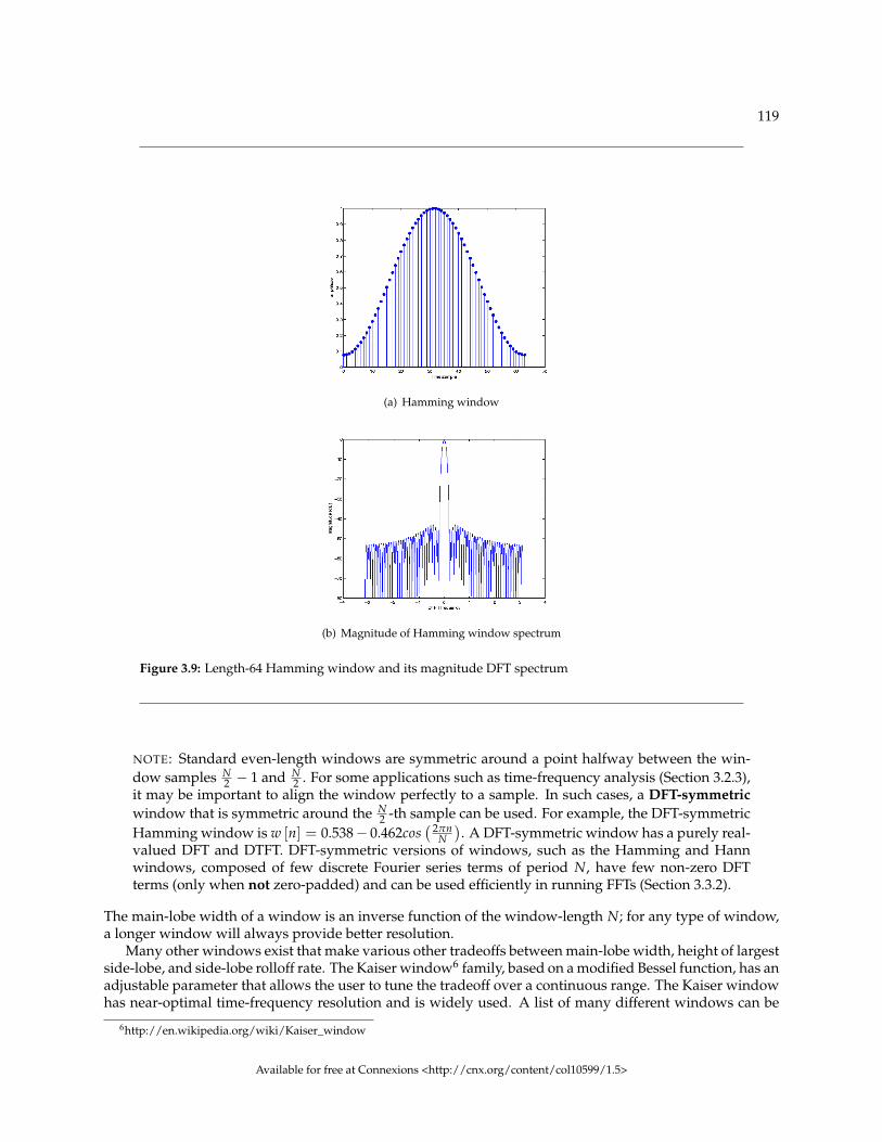
119
(a) Hamming window
(b) Magnitude of Hamming window spectrum
Figure 3.9: Length-64 Hamming window and its magnitude DFT spectrum
NOTE: Standard even-length windows are symmetric around a point halfway between the win-dow samples N
2 − 1 and N2 . For some applications such as time-frequency analysis (Section 3.2.3),
it may be important to align the window perfectly to a sample. In such cases, a DFT-symmetricwindow that is symmetric around the N
2 -th sample can be used. For example, the DFT-symmetricHamming window is w [n] = 0.538− 0.462cos
( 2πnN). A DFT-symmetric window has a purely real-
valued DFT and DTFT. DFT-symmetric versions of windows, such as the Hamming and Hannwindows, composed of few discrete Fourier series terms of period N, have few non-zero DFTterms (only when not zero-padded) and can be used efficiently in running FFTs (Section 3.3.2).
The main-lobe width of a window is an inverse function of the window-length N; for any type of window,a longer window will always provide better resolution.
Many other windows exist that make various other tradeoffs between main-lobe width, height of largestside-lobe, and side-lobe rolloff rate. The Kaiser window6 family, based on a modified Bessel function, has anadjustable parameter that allows the user to tune the tradeoff over a continuous range. The Kaiser windowhas near-optimal time-frequency resolution and is widely used. A list of many different windows can be
6http://en.wikipedia.org/wiki/Kaiser_window
Available for free at Connexions <http://cnx.org/content/col10599/1.5>

120 CHAPTER 3. THE DFT, FFT, AND PRACTICAL SPECTRAL ANALYSIS
found here7 .
Example 3.1Figure 3.10 shows 64 samples of a real-valued signal composed of several sinusoids of various
frequencies and amplitudes.
Figure 3.10: 64 samples of an unknown signal
Figure 3.11 shows the magnitude (in dB) of the positive frequencies of a length-1024 zero-padded DFT of this signal (that is, using a simple truncation, or rectangular, window).
7http://en.wikipedia.org/wiki/Window_function
Available for free at Connexions <http://cnx.org/content/col10599/1.5>

121
Figure 3.11: Magnitude (in dB) of the zero-padded DFT spectrum of the signal in Figure 3.10 using a simplelength-64 rectangular window
From this spectrum, it is clear that the signal has two large, nearby frequency components withfrequencies near 1 radian of essentially the same magnitude.
Figure 3.12 shows the spectral estimate produced using a length-64 Hamming window appliedto the same signal shown in Figure 3.10.
Available for free at Connexions <http://cnx.org/content/col10599/1.5>

122 CHAPTER 3. THE DFT, FFT, AND PRACTICAL SPECTRAL ANALYSIS
Figure 3.12: Magnitude (in dB) of the zero-padded DFT spectrum of the signal in Figure 3.10 using alength-64 Hamming window
The two large spectral peaks can no longer be resolved; they blur into a single broad peak dueto the reduced spectral resolution of the broader main lobe of the Hamming window. However, thelower side-lobes reveal a third component at a frequency of about 0.7 radians at about 35 dB lowermagnitude than the larger components. This component was entirely buried under the side-lobeswhen the rectangular window was used, but now stands out well above the much lower nearbyside-lobes of the Hamming window.
Figure 3.13 shows the spectral estimate produced using a length-64 Hann window applied tothe same signal shown in Figure 3.10.
Available for free at Connexions <http://cnx.org/content/col10599/1.5>

123
Figure 3.13: Magnitude (in dB) of the zero-padded DFT spectrum of the signal in Figure 3.10 using alength-64 Hann window
The two large components again merge into a single peak, and the smaller component ob-served with the Hamming window is largely lost under the higher nearby side-lobes of the Hannwindow. However, due to the much faster side-lobe rolloff of the Hann window’s spectrum, afourth component at a frequency of about 2.5 radians with a magnitude about 65 dB below that ofthe main peaks is now clearly visible.
This example illustrates that no single window is best for all spectrum analyses. The bestwindow depends on the nature of the signal, and different windows may be better for differentcomponents of the same signal. A skilled spectrum analysist may apply several different windowsto a signal to gain a fuller understanding of the data.
3.2.2 Classical Statistical Spectral Estimation8
Many signals are either partly or wholly stochastic, or random. Important examples include human speech,vibration in machines, and CDMA9 communication signals. Given the ever-present noise in electronic
8This content is available online at <http://cnx.org/content/m12014/1.3/>.9http://en.wikipedia.org/wiki/Cdma
Available for free at Connexions <http://cnx.org/content/col10599/1.5>

124 CHAPTER 3. THE DFT, FFT, AND PRACTICAL SPECTRAL ANALYSIS
systems, it can be argued that almost all signals are at least partly stochastic. Such signals may have adistinct average spectral structure that reveals important information (such as for speech recognition orearly detection of damage in machinery). Spectrum analysis of any single block of data using window-based deterministic spectrum analysis (Section 3.2.1), however, produces a random spectrum that may bedifficult to interpret. For such situations, the classical statistical spectrum estimation methods described inthis module can be used.
The goal in classical statistical spectrum analysis is to estimate E[(|X (ω) |)2
], the power spectral den-
sity (PSD) across frequency of the stochastic signal. That is, the goal is to find the expected (mean, or aver-age) energy density of the signal as a function of frequency. (For zero-mean signals, this equals the varianceof each frequency sample.) Since the spectrum of each block of signal samples is itself random, we mustaverage the squared spectral magnitudes over a number of blocks of data to find the mean. There are twomain classical approaches, the periodogram (Section 3.2.2.1: Periodogram method) and auto-correlation(Section 3.2.2.2: Auto-correlation-based approach) methods.
3.2.2.1 Periodogram method
The periodogram method divides the signal into a number of shorter (and often overlapped) blocks of data,computes the squared magnitude of the windowed (Section 3.2.1.6: Effects of Windowing) (and usuallyzero-padded (Section 3.2.1.5: Zero-Padding)) DFT (3.5), Xi (ωk), of each block, and averages them to esti-mate the power spectral density. The squared magnitudes of the DFTs of L possibly overlapped length-Nwindowed blocks of signal (each probably with zero-padding (Section 3.2.1.5: Zero-Padding)) are averagedto estimate the power spectral density:
X (ωk) =1L
L
∑i=1
(|Xi (ωk) |)2
For a fixed total number of samples, this introduces a tradeoff: Larger individual data blocks providesbetter frequency resolution due to the use of a longer window, but it means there are less blocks to average,so the estimate has higher variance and appears more noisy. The best tradeoff depends on the application.Overlapping blocks by a factor of two to four increases the number of averages and reduces the variance,but since the same data is being reused, still more overlapping does not further reduce the variance. As withany window-based spectrum estimation (Section 3.2.1.6: Effects of Windowing) procedure, the windowfunction introduces broadening and sidelobes into the power spectrum estimate. That is, the periodogram
produces an estimate of the windowed spectrum X (ω) = E[(|X (ω) ∗WM|)2
], not of E
[(|X (ω) |)2
].
Example 3.2Figure 3.14 shows the non-negative frequencies of the DFT (zero-padded to 1024 total samples) of64 samples of a real-valued stochastic signal.
Available for free at Connexions <http://cnx.org/content/col10599/1.5>

125
Figure 3.14: DFT magnitude (in dB) of 64 samples of a stochastic signal
With no averaging, the power spectrum is very noisy and difficult to interpret other than notinga significant reduction in spectral energy above about half the Nyquist frequency. Various peaksand valleys appear in the lower frequencies, but it is impossible to say from this figure whetherthey represent actual structure in the power spectral density (PSD) or simply random variation inthis single realization. Figure 3.15 shows the same frequencies of a length-1024 DFT of a length-1024 signal. While the frequency resolution has improved, there is still no averaging, so it remainsdifficult to understand the power spectral density of this signal. Certain small peaks in frequencymight represent narrowband components in the spectrum, or may just be random noise peaks.
Available for free at Connexions <http://cnx.org/content/col10599/1.5>

126 CHAPTER 3. THE DFT, FFT, AND PRACTICAL SPECTRAL ANALYSIS
Figure 3.15: DFT magnitude (in dB) of 1024 samples of a stochastic signal
In Figure 3.16, a power spectral density computed from averaging the squared magnitudes oflength-1024 zero-padded DFTs of 508 length-64 blocks of data (overlapped by a factor of four, or a16-sample step between blocks) are shown.
Available for free at Connexions <http://cnx.org/content/col10599/1.5>

127
Figure 3.16: Power spectrum density estimate (in dB) of 1024 samples of a stochastic signal
While the frequency resolution corresponds to that of a length-64 truncation window, the aver-aging greatly reduces the variance of the spectral estimate and allows the user to reliably concludethat the signal consists of lowpass broadband noise with a flat power spectrum up to half theNyquist frequency, with a stronger narrowband frequency component at around 0.65 radians.
3.2.2.2 Auto-correlation-based approach
The averaging necessary to estimate a power spectral density can be performed in the discrete-time domain,rather than in frequency, using the auto-correlation method. The squared magnitude of the frequency re-sponse, from the DTFT multiplication and conjugation properties, corresponds in the discrete-time domainto the signal convolved with the time-reverse of itself,
(|X (ω) |)2 = X (ω) X∗ (ω)↔ (x (n) , x∗ (−n)) = r (n)
or its auto-correlationr (n) = ∑
kx (k) x∗ (n + k)
Available for free at Connexions <http://cnx.org/content/col10599/1.5>

128 CHAPTER 3. THE DFT, FFT, AND PRACTICAL SPECTRAL ANALYSIS
We can thus compute the squared magnitude of the spectrum of a signal by computing the DFT of its auto-correlation. For stochastic signals, the power spectral density is an expectation, or average, and by linearityof expectation can be found by transforming the average of the auto-correlation. For a finite block of Nsignal samples, the average of the autocorrelation values, r (n), is
r (n) =1
N − n
N−(1−n)
∑k=0
x (k) x∗ (n + k)
Note that with increasing lag, n, fewer values are averaged, so they introduce more noise into the esti-mated power spectrum. By windowing (Section 3.2.1.6: Effects of Windowing) the auto-correlation beforetransforming it to the frequency domain, a less noisy power spectrum is obtained, at the expense of less res-olution. The multiplication property of the DTFT shows that the windowing smooths the resulting powerspectrum via convolution with the DTFT of the window:
X (ω) =M
∑n=−M
r (n) w (n) e−(jωn) =(
E[(|X (ω) |)2
])∗W (ω)
This yields another important interpretation of how the auto-correlation method works: it estimates thepower spectral density by averaging the power spectrum over nearby frequencies, through convolutionwith the window function’s transform, to reduce variance. Just as with the periodogram approach, there isalways a variance vs. resolution tradeoff. The periodogram and the auto-correlation method give similarresults for a similar amount of averaging; the user should simply note that in the periodogram case, thewindow introduces smoothing of the spectrum via frequency convolution before squaring the magnitude,whereas the periodogram convolves the squared magnitude with W (ω).
3.2.3 Short Time Fourier Transform10
3.2.3.1 Short Time Fourier Transform
The Fourier transforms (FT, DTFT, DFT, etc.) do not clearly indicate how the frequency content of a signalchanges over time.
That information is hidden in the phase - it is not revealed by the plot of the magnitude of the spectrum.
NOTE: To see how the frequency content of a signal changes over time, we can cut the signal intoblocks and compute the spectrum of each block.
To improve the result,
1. blocks are overlapping2. each block is multiplied by a window that is tapered at its endpoints.
Several parameters must be chosen:
• Block length, R.• The type of window.• Amount of overlap between blocks. (Figure 3.17 (STFT: Overlap Parameter))• Amount of zero padding, if any.
10This content is available online at <http://cnx.org/content/m10570/2.4/>.
Available for free at Connexions <http://cnx.org/content/col10599/1.5>

129
STFT: Overlap Parameter
Figure 3.17
The short-time Fourier transform is defined as
X (ω, m) = STFT (x (n)) := DTFT (x (n−m) w (n))
= ∑∞n=−∞ x (n−m) w (n) e−(jωn)
= ∑R−1n=0 x (n−m) w (n) e−(jωn)
(3.9)
where w (n) is the window function of length R.
Available for free at Connexions <http://cnx.org/content/col10599/1.5>

130 CHAPTER 3. THE DFT, FFT, AND PRACTICAL SPECTRAL ANALYSIS
1. The STFT of a signal x (n) is a function of two variables: time and frequency.2. The block length is determined by the support of the window function w (n).3. A graphical display of the magnitude of the STFT, |X (ω, m) |, is called the spectrogram of the signal.
It is often used in speech processing.4. The STFT of a signal is invertible.5. One can choose the block length. A long block length will provide higher frequency resolution (be-
cause the main-lobe of the window function will be narrow). A short block length will provide highertime resolution because less averaging across samples is performed for each STFT value.
6. A narrow-band spectrogram is one computed using a relatively long block length R, (long windowfunction).
7. A wide-band spectrogram is one computed using a relatively short block length R, (short windowfunction).
3.2.3.1.1 Sampled STFT
To numerically evaluate the STFT, we sample the frequency axis ω in N equally spaced samples from ω = 0to ω = 2π.
ωk =2π
Nk , 0 ≤ k ≤ N − 1 (3.10)
We then have the discrete STFT,
Xd (k, m) := X( 2π
N k, m)
= ∑R−1n=0 x (n−m) w (n) e−(jωn)
= ∑R−1n=0 x (n−m) w (n) WN
−(kn)
= DFTN
(x (n−m) w (n) |R−1
n=0 , 0,. . .0) (3.11)
where 0,. . .0 is N − R.In this definition, the overlap between adjacent blocks is R− 1. The signal is shifted along the window
one sample at a time. That generates more points than is usually needed, so we also sample the STFT alongthe time direction. That means we usually evaluate
Xd (k, Lm)
where L is the time-skip. The relation between the time-skip, the number of overlapping samples, and theblock length is
Overlap = R− L
Exercise 3.2.3.1 (Solution on p. 184.)Match each signal to its spectrogram in Figure 3.18.
Available for free at Connexions <http://cnx.org/content/col10599/1.5>

131
(a)
(b)
Figure 3.18
Available for free at Connexions <http://cnx.org/content/col10599/1.5>

132 CHAPTER 3. THE DFT, FFT, AND PRACTICAL SPECTRAL ANALYSIS
3.2.3.1.2 Spectrogram Example
Figure 3.19
Available for free at Connexions <http://cnx.org/content/col10599/1.5>

133
Figure 3.20
The matlab program for producing the figures above (Figure 3.19 and Figure 3.20).
% LOAD DATA
load mtlb;
x = mtlb;
figure(1), clf
plot(0:4000,x)
xlabel('n')
ylabel('x(n)')
% SET PARAMETERS
R = 256; % R: block length
window = hamming(R); % window function of length R
N = 512; % N: frequency discretization
L = 35; % L: time lapse between blocks
fs = 7418; % fs: sampling frequency
Available for free at Connexions <http://cnx.org/content/col10599/1.5>

134 CHAPTER 3. THE DFT, FFT, AND PRACTICAL SPECTRAL ANALYSIS
overlap = R - L;
% COMPUTE SPECTROGRAM
[B,f,t] = specgram(x,N,fs,window,overlap);
% MAKE PLOT
figure(2), clf
imagesc(t,f,log10(abs(B)));
colormap('jet')
axis xy
xlabel('time')
ylabel('frequency')
title('SPECTROGRAM, R = 256')
Available for free at Connexions <http://cnx.org/content/col10599/1.5>

135
3.2.3.1.3 Effect of window length R
Narrow-band spectrogram: better frequency resolution
Figure 3.21
Available for free at Connexions <http://cnx.org/content/col10599/1.5>

136 CHAPTER 3. THE DFT, FFT, AND PRACTICAL SPECTRAL ANALYSIS
Wide-band spectrogram: better time resolution
Figure 3.22
Here is another example to illustrate the frequency/time resolution trade-off (See figures - Figure 3.21(Narrow-band spectrogram: better frequency resolution), Figure 3.22 (Wide-band spectrogram: better timeresolution), and Figure 3.23 (Effect of Window Length R)).
Available for free at Connexions <http://cnx.org/content/col10599/1.5>

137
Effect of Window Length R
(a)
(b)
Figure 3.23
3.2.3.1.4 Effect of L and N
A spectrogram is computed with different parameters:
L ∈ 1, 10
N ∈ 32, 256
• L = time lapse between blocks.• N = FFT length (Each block is zero-padded to length N.)
In each case, the block length is 30 samples.Exercise 3.2.3.2 (Solution on p. 184.)For each of the four spectrograms in Figure 3.24 can you tell what L and N are?
Available for free at Connexions <http://cnx.org/content/col10599/1.5>

138 CHAPTER 3. THE DFT, FFT, AND PRACTICAL SPECTRAL ANALYSIS
(a)
(b)
Figure 3.24
L and N do not effect the time resolution or the frequency resolution. They only affect the ’pixelation’.
3.2.3.1.5 Effect of R and L
Shown below are four spectrograms of the same signal. Each spectrogram is computed using a different setof parameters.
R ∈ 120, 256, 1024
L ∈ 35, 250
where
• R = block length• L = time lapse between blocks.
Exercise 3.2.3.3 (Solution on p. 184.)For each of the four spectrograms in Figure 3.25, match the above values of L and R.
Available for free at Connexions <http://cnx.org/content/col10599/1.5>

139
Figure 3.25
If you like, you may listen to this signal with the soundsc command; the data is in the file: stft_data.m.Here (Figure 3.26) is a figure of the signal.
Available for free at Connexions <http://cnx.org/content/col10599/1.5>

140 CHAPTER 3. THE DFT, FFT, AND PRACTICAL SPECTRAL ANALYSIS
Figure 3.26
3.3 Fast Fourier Transform Algorithms
3.3.1 Overview of Fast Fourier Transform (FFT) Algorithms11
A fast Fourier transform12, or FFT13, is not a new transform, but is a computationally efficient algorithm forthe computing the DFT (Section 3.1.1). The length-N DFT, defined as
X (k) =N−1
∑n=0
x (n) e−(j 2πnkN ) (3.12)
where X (k) and x (n) are in general complex-valued and 0 ≤ k, n ≤ N− 1, requires N complex multipliesto compute each X (k). Direct computation of all N frequency samples thus requires N2 complex multiplies
and N (N − 1) complex additions. (This assumes precomputation of the DFT coefficients WnkN
.= e−(j 2πnkN );
otherwise, the cost is even higher.) For the large DFT lengths used in many applications, N2 operations maybe prohibitive. (For example, digital terrestrial television broadcast in Europe uses N = 2048 or 8192 OFDMchannels, and the SETI14 project uses up to length-4194304 DFTs.) DFTs are thus almost always computedin practice by an FFT algorithm15. FFTs are very widely used in signal processing, for applications such asspectrum analysis (Section 3.2.1) and digital filtering via fast convolution (Section 3.4).
3.3.1.1 History of the FFT
It is now known that C.F. Gauss16 invented an FFT in 1805 or so to assist the computation of planetaryorbits via discrete Fourier series. Various FFT algorithms were independently invented over the next twocenturies, but FFTs achieved widespread awareness and impact only with the Cooley and Tukey algorithmpublished in 1965, which came at a time of increasing use of digital computers and when the vast rangeof applications of numerical Fourier techniques was becoming apparent. Cooley and Tukey’s algorithmspawned a surge of research in FFTs and was also partly responsible for the emergence of Digital Signal
11This content is available online at <http://cnx.org/content/m12026/1.3/>.12The DFT, FFT, and Practical Spectral Analysis <http://cnx.org/content/col10281/latest/>13The DFT, FFT, and Practical Spectral Analysis <http://cnx.org/content/col10281/latest/>14http://en.wikipedia.org/wiki/SETI15The DFT, FFT, and Practical Spectral Analysis <http://cnx.org/content/col10281/latest/>16http://en.wikipedia.org/wiki/Carl_Friedrich_Gauss
Available for free at Connexions <http://cnx.org/content/col10599/1.5>

141
Processing (DSP) as a distinct, recognized discipline. Since then, many different algorithms have beenrediscovered or developed, and efficient FFTs now exist for all DFT lengths.
Available for free at Connexions <http://cnx.org/content/col10599/1.5>

142 CHAPTER 3. THE DFT, FFT, AND PRACTICAL SPECTRAL ANALYSIS
3.3.1.2 Summary of FFT algorithms
The main strategy behind most FFT algorithms is to factor a length-N DFT into a number of shorter-lengthDFTs, the outputs of which are reused multiple times (usually in additional short-length DFTs!) to computethe final results. The lengths of the short DFTs correspond to integer factors of the DFT length, N, lead-ing to different algorithms for different lengths and factors. By far the most commonly used FFTs selectN = 2M to be a power of two, leading to the very efficient power-of-two FFT algorithms (Section 3.3.4.1),including the decimation-in-time radix-2 FFT (Section 3.3.4.2.1) and the decimation-in-frequency radix-2FFT (Section 3.3.4.2.2) algorithms, the radix-4 FFT (Section 3.3.4.3) (N = 4M), and the split-radix FFT (Sec-tion 3.3.4.4). Power-of-two algorithms gain their high efficiency from extensive reuse of intermediate resultsand from the low complexity of length-2 and length-4 DFTs, which require no multiplications. Algorithmsfor lengths with repeated common factors17 (such as 2 or 4 in the radix-2 and radix-4 algorithms, respec-tively) require extra twiddle factor multiplications between the short-length DFTs, which together lead to acomputational complexity of O (NlogN), a very considerable savings over direct computation of the DFT.
The other major class of algorithms is the Prime-Factor Algorithms (PFA)18. In PFAs, the short-lengthDFTs must be of relatively prime lengths. These algorithms gain efficiency by reuse of intermediate com-putations and by eliminating twiddle-factor multiplies, but require more operations than the power-of-twoalgorithms to compute the short DFTs of various prime lengths. In the end, the computational costs of theprime-factor and the power-of-two algorithms are comparable for similar lengths, as illustrated in Choosingthe Best FFT Algorithm (Section 3.7). Prime-length DFTs cannot be factored into shorter DFTs, but in differ-ent ways both Rader’s conversion (Section 3.6) and the chirp z-transform (Section 3.5) convert prime-lengthDFTs into convolutions of other lengths that can be computed efficiently using FFTs via fast convolution(Section 3.4).
Some applications require only a few DFT frequency samples, in which case Goertzel’s algorithm (Sec-tion 3.3.3) halves the number of computations relative to the DFT sum. Other applications involve succes-sive DFTs of overlapped blocks of samples, for which the running FFT (Section 3.3.2) can be more efficientthan separate FFTs of each block.
3.3.2 Running FFT19
Some applications need DFT (3.5) frequencies of the most recent N samples on an ongoing basis. Oneexample is DTMF20 , or touch-tone telephone dialing, in which a detection circuit must constantly monitorthe line for two simultaneous frequencies indicating that a telephone button is depressed. In such cases,most of the data in each successive block of samples is the same, and it is possible to efficiently updatethe DFT value from the previous sample to compute that of the current sample. Figure 3.27 illustratessuccessive length-4 blocks of data for which successive DFT values may be needed. The running FFTalgorithm described here can be used to compute successive DFT values at a cost of only two complexmultiplies and additions per DFT frequency.
17"Multidimensional Index Maps" <http://cnx.org/content/m12025/latest/>18"The Prime Factor Algorithm" <http://cnx.org/content/m12033/latest/>19This content is available online at <http://cnx.org/content/m12029/1.5/>.20http://en.wikipedia.org/wiki/DTMF
Available for free at Connexions <http://cnx.org/content/col10599/1.5>

143
Figure 3.27: The running FFT efficiently computes DFT values for successive overlapped blocks of samples.
The running FFT algorithm is derived by expressing each DFT sample, Xn+1 (ωk), for the next block attime n + 1 in terms of the previous value, Xn (ωk), at time n.
Xn (ωk) =N−1
∑p=0
x (n− p) e−(jωk p)
Xn+1 (ωk) =N−1
∑p=0
x (n + 1− p) e−(jωk p)
Let q = p− 1:
Xn+1 (ωk) =N−2
∑q=−1
x (n− q) e−(jωk(q−1)) = ejωkN−2
∑q=0
x (n− q) e−(jωkq) + x (n + 1)
Now let’s add and subtract e−(jωk(N−2))x (n− N + 1):
Xn+1 (ωk) = ejωk ∑N−2q=0 x (n− q) e−(jωkq) + ejωk x (n− (N − 1)) e−(jωk(N−1)) −
e−(jωk(N−2))x (n− N + 1) + x (n + 1) = ejωk ∑N−1q=0 x (n− q) e−(jωk) + x (n + 1)−
e−(jωk)x (n− N + 1) = ejωk Xn (ωk) + x (n + 1)− e−(jωk(N−2))x (n− N + 1)
(3.13)
This running FFT algorithm requires only two complex multiplies and adds per update, rather than Nif each DFT value were recomputed according to the DFT equation. Another advantage of this algorithm isthat it works for any ωk, rather than just the standard DFT frequencies. This can make it advantageous forapplications, such as DTMF detection, where only a few arbitrary frequencies are needed.
Successive computation of a specific DFT frequency for overlapped blocks can also be thought of as alength-N FIR filter21. The running FFT is an efficient recursive implementation of this filter for this specialcase. Figure 3.28 shows a block diagram of the running FFT algorithm. The running FFT is one way tocompute DFT filterbanks (Section 5.6). If a window other than rectangular is desired, a running FFT requireseither a fast recursive implementation of the corresponding windowed, modulated impulse response, or itmust have few non-zero coefficients so that it can be applied after the running FFT update via frequency-domain convolution. DFT-symmmetric raised-cosine windows (Section 3.2.1.6: Effects of Windowing) arean example.
21Digital Filter Design <http://cnx.org/content/col10285/latest/>
Available for free at Connexions <http://cnx.org/content/col10599/1.5>

144 CHAPTER 3. THE DFT, FFT, AND PRACTICAL SPECTRAL ANALYSIS
Figure 3.28: Block diagram of the running FFT computation, implemented as a recursive filter
3.3.3 Goertzel’s Algorithm22
Some applications require only a few DFT frequencies. One example is frequency-shift keying (FSK)23
demodulation, in which typically two frequencies are used to transmit binary data; another example isDTMF24 , or touch-tone telephone dialing, in which a detection circuit must constantly monitor the linefor two simultaneous frequencies indicating that a telephone button is depressed. Goertzel’s algorithm[13]reduces the number of real-valued multiplications by almost a factor of two relative to direct computationvia the DFT equation (3.5). Goertzel’s algorithm is thus useful for computing a few frequency values; ifmany or most DFT values are needed, FFT algorithms (Section 3.3.1) that compute all DFT samples inO (NlogN) operations are faster. Goertzel’s algorithm can be derived by converting the DFT equation(Section 3.1.1) into an equivalent form as a convolution, which can be efficiently implemented as a digital
filter. For increased clarity, in the equations below the complex exponential is denoted as e−(j 2πkN ) = Wk
N .Note that because W−Nk
N always equals 1, the DFT equation (Section 3.1.1) can be rewritten as a convolution,or filtering operation:
X (k) = ∑N−1n=0 x (n) 1Wnk
N
= ∑N−1n=0 x (n) W−Nk
N WnkN
= ∑N−1n=0 x (n) W(N−n)(−k)
N
=(((
W−kN x (0) + x (1)
)W−k
N + x (2))
W−kN + · · ·+ x (N − 1)
)W−k
N
(3.14)
Note that this last expression can be written in terms of a recursive difference equation (Section 1.9.1)
y (n) = W−kN y (n− 1) + x (n)
where y (−1) = 0. The DFT coefficient equals the output of the difference equation at time n = N:
X (k) = y (N)22This content is available online at <http://cnx.org/content/m12024/1.5/>.23http://en.wikipedia.org/wiki/Frequency-shift_keying24http://en.wikipedia.org/wiki/DTMF
Available for free at Connexions <http://cnx.org/content/col10599/1.5>

145
Expressing the difference equation as a z-transform (Section 1.9.1) and multiplying both numerator anddenominator by 1−Wk
Nz−1 gives the transfer function
Y (z)X (z)
= H (z) =1
1−W−kN z−1
=1−Wk
Nz−1
1−((
WkN + W−k
N
)z−1 − z−2
) =1−Wk
Nz−1
1−(
2cos(
2πkN
)z−1 − z−2
)This system can be realized by the structure in Figure 3.29
Figure 3.29
We want y (n) not for all n, but only for n = N. We can thus compute only the recursive part, or justthe left side of the flow graph in Figure 3.29, for n = [0, 1, . . . , N], which involves only a real/complexproduct rather than a complex/complex product as in a direct DFT (3.5), plus one complex multiply to gety (N) = X (k).
NOTE: The input x (N) at time n = N must equal 0! A slightly more efficient alternate imple-mentation25 that computes the full recursion only through n = N − 1 and combines the nonzerooperations of the final recursion with the final complex multiply can be found here26 , completewith pseudocode (for real-valued data).
If the data are real-valued, only real/real multiplications and real additions are needed until the final mul-tiply.
NOTE: The computational cost of Goertzel’s algorithm is thus 2N + 2 real multiplies and 4N − 2real adds, a reduction of almost a factor of two in the number of real multiplies relative to directcomputation via the DFT equation. If the data are real-valued, this cost is almost halved again.
For certain frequencies, additional simplifications requiring even fewer multiplications are possible.(For example, for the DC (k = 0) frequency, all the multipliers equal 1 and only additions are needed.)A correspondence by C.G. Boncelet, Jr.[6] describes some of these additional simplifications. Once again,
25http://www.mstarlabs.com/dsp/goertzel/goertzel.html26http://www.mstarlabs.com/dsp/goertzel/goertzel.html
Available for free at Connexions <http://cnx.org/content/col10599/1.5>

146 CHAPTER 3. THE DFT, FFT, AND PRACTICAL SPECTRAL ANALYSIS
Goertzel’s and Boncelet’s algorithms are efficient for a few DFT frequency samples; if more than logN fre-quencies are needed, O (NlogN) FFT algorithms (Section 3.3.1) that compute all frequencies simultaneouslywill be more efficient.
3.3.4 Power-of-Two FFTs
3.3.4.1 Power-of-two FFTs27
FFTs of length N = 2M equal to a power of two are, by far, the most commonly used. These algorithms arevery efficient, relatively simple, and a single program can compute power-of-two FFTs of different lengths.As with most FFT algorithms, they gain their efficiency by computing all DFT (Section 3.1.1) points si-multaneously through extensive reuse of intermediate computations; they are thus efficient when manyDFT frequency samples are needed. The simplest power-of-two FFTs are the decimation-in-time radix-2 FFT (Section 3.3.4.2.1) and the decimation-in-frequency radix-2 FFT (Section 3.3.4.2.2); they reduce thelength-N = 2M DFT to a series of length-2 DFT computations with twiddle-factor complex multiplicationsbetween them. The radix-4 FFT algorithm (Section 3.3.4.3) similarly reduces a length-N = 4M DFT to aseries of length-4 DFT computations with twiddle-factor multiplies in between. Radix-4 FFTs require only75% as many complex multiplications as the radix-2 algorithms, although the number of complex addi-tions remains the same. Radix-8 and higher-radix FFT algorithms can be derived using multi-dimensionalindex maps28 to reduce the computational complexity a bit more. However, the split-radix algorithm (Sec-tion 3.3.4.4) and its recent extensions combine the best elements of the radix-2 and radix-4 algorithms toobtain lower complexity than either or than any higher radix, requiring only two-thirds as many complexmultiplies as the radix-2 algorithms. All of these algorithms obtain huge savings over direct computationof the DFT, reducing the complexity from O
(N2) to O (NlogN).
The efficiency of an FFT implementation depends on more than just the number of computations. Effi-cient FFT programming tricks (Section 3.3.5) can make up to a several-fold difference in the run-time of FFTprograms. Alternate FFT structures (Section 3.3.4.2.3) can lead to a more convenient data flow for certainhardware. As discussed in choosing the best FFT algorithm (Section 3.7), certain hardware is designed for,and thus most efficient for, FFTs of specific lengths or radices.
3.3.4.2 Radix-2 Algorithms
3.3.4.2.1 Decimation-in-time (DIT) Radix-2 FFT29
The radix-2 decimation-in-time and decimation-in-frequency (Section 3.3.4.2.2) fast Fourier transforms(FFTs) are the simplest FFT algorithms (Section 3.3.1). Like all FFTs, they gain their speed by reusing theresults of smaller, intermediate computations to compute multiple DFT frequency outputs.
3.3.4.2.1.1 Decimation in time
The radix-2 decimation-in-time algorithm rearranges the discrete Fourier transform (DFT) equation (Sec-tion 3.1.1) into two parts: a sum over the even-numbered discrete-time indices n = [0, 2, 4, . . . , N − 2] and a
27This content is available online at <http://cnx.org/content/m12059/1.2/>.28"Multidimensional Index Maps" <http://cnx.org/content/m12025/latest/>29This content is available online at <http://cnx.org/content/m12016/1.7/>.
Available for free at Connexions <http://cnx.org/content/col10599/1.5>

147
sum over the odd-numbered indices n = [1, 3, 5, . . . , N − 1] as in (3.15):
X (k) = ∑N−1n=0 x (n) e−(j 2πnk
N )
= ∑N2 −1
n=0 x (2n) e−(
j 2π×(2n)kN
)+ ∑
N2 −1
n=0 x (2n + 1) e−(
j 2π(2n+1)kN
)
= ∑N2 −1
n=0 x (2n) e−(
j 2πnkN2
)+ e−(j 2πk
N ) ∑N2 −1
n=0 x (2n + 1) e−(
j 2πnkN2
)
= DFT N2
[[x (0) , x (2) , . . . , x (N − 2)]] + WkN DFT N
2[[x (1) , x (3) , . . . , x (N − 1)]]
(3.15)
The mathematical simplifications in (3.15) reveal that all DFT frequency outputs X (k) can be computed asthe sum of the outputs of two length- N
2 DFTs, of the even-indexed and odd-indexed discrete-time samples,respectively, where the odd-indexed short DFT is multiplied by a so-called twiddle factor term Wk
N =
e−(j 2πkN ). This is called a decimation in time because the time samples are rearranged in alternating groups,
and a radix-2 algorithm because there are two groups. Figure 3.30 graphically illustrates this form of theDFT computation, where for convenience the frequency outputs of the length- N
2 DFT of the even-indexedtime samples are denoted G (k) and those of the odd-indexed samples as H (k). Because of the periodicitywith N
2 frequency samples of these length- N2 DFTs, G (k) and H (k) can be used to compute two of the
length-N DFT frequencies, namely X (k) and X(
k + N2
), but with a different twiddle factor. This reuse of
these short-length DFT outputs gives the FFT its computational savings.
Figure 3.30: Decimation in time of a length-N DFT into two length- N2 DFTs followed by a combining stage.
Whereas direct computation of all N DFT frequencies according to the DFT equation (Section 3.1.1)would require N2 complex multiplies and N2−N complex additions (for complex-valued data), by reusingthe results of the two short-length DFTs as illustrated in Figure 3.30, the computational cost is now
Available for free at Connexions <http://cnx.org/content/col10599/1.5>

148 CHAPTER 3. THE DFT, FFT, AND PRACTICAL SPECTRAL ANALYSIS
New Operation Counts
• 2(
N2
)2+ N = N2
2 + N complex multiplies
• 2 N2
(N2 − 1
)+ N = N2
2 complex additions
This simple reorganization and reuse has reduced the total computation by almost a factor of two overdirect DFT (Section 3.1.1) computation!
3.3.4.2.1.2 Additional Simplification
A basic butterfly operation is shown in Figure 3.31, which requires only N2 twiddle-factor multiplies per
stage. It is worthwhile to note that, after merging the twiddle factors to a single term on the lower branch,the remaining butterfly is actually a length-2 DFT! The theory of multi-dimensional index maps30 showsthat this must be the case, and that FFTs of any factorable length may consist of successive stages of shorter-length FFTs with twiddle-factor multiplications in between.
(a) (b)
Figure 3.31: Radix-2 DIT butterfly simplification: both operations produce the same outputs
3.3.4.2.1.3 Radix-2 decimation-in-time FFT
The same radix-2 decimation in time can be applied recursively to the two length N2 DFT (Section 3.1.1)s to
save computation. When successively applied until the shorter and shorter DFTs reach length-2, the resultis the radix-2 DIT FFT algorithm (Figure 3.32).
30"Multidimensional Index Maps" <http://cnx.org/content/m12025/latest/>
Available for free at Connexions <http://cnx.org/content/col10599/1.5>

149
Figure 3.32: Radix-2 Decimation-in-Time FFT algorithm for a length-8 signal
The full radix-2 decimation-in-time decomposition illustrated in Figure 3.32 using the simplified butter-flies (Figure 3.31) involves M = log2N stages, each with N
2 butterflies per stage. Each butterfly requires 1complex multiply and 2 adds per butterfly. The total cost of the algorithm is thusComputational cost of radix-2 DIT FFT
• N2 log2N complex multiplies
• Nlog2N complex adds
This is a remarkable savings over direct computation of the DFT. For example, a length-1024 DFT wouldrequire 1048576 complex multiplications and 1047552 complex additions with direct computation, but only5120 complex multiplications and 10240 complex additions using the radix-2 FFT, a savings by a factor of100 or more. The relative savings increase with longer FFT lengths, and are less for shorter lengths.
Modest additional reductions in computation can be achieved by noting that certain twiddle factors,
namely Using special butterflies for W0N , W
N2
N , WN4
N , WN8
N , W3N8
N , require no multiplications, or fewer realmultiplies than other ones. By implementing special butterflies for these twiddle factors as discussed inFFT algorithm and programming tricks, the computational cost of the radix-2 decimation-in-time FFT canbe reduced to
• 2Nlog2N − 7N + 12 real multiplies• 3Nlog2N − 3N + 4 real additions
NOTE: In a decimation-in-time radix-2 FFT as illustrated in Figure 3.32, the input is in bit-reversedorder (hence "decimation-in-time"). That is, if the time-sample index n is written as a binary num-ber, the order is that binary number reversed. The bit-reversal process is illustrated for a length-N = 8 example below.
Example 3.3: N=8
Available for free at Connexions <http://cnx.org/content/col10599/1.5>

150 CHAPTER 3. THE DFT, FFT, AND PRACTICAL SPECTRAL ANALYSIS
In-order index In-order index in binary Bit-reversed binary Bit-reversed index
0 000 000 0
1 001 100 4
2 010 010 2
3 011 110 6
4 100 001 1
5 101 101 5
6 110 011 3
7 111 111 7
Table 3.1
It is important to note that, if the input signal data are placed in bit-reversed order before beginning theFFT computations, the outputs of each butterfly throughout the computation can be placed in the samememory locations from which the inputs were fetched, resulting in an in-place algorithm that requires noextra memory to perform the FFT. Most FFT implementations are in-place, and overwrite the input datawith the intermediate values and finally the output.
3.3.4.2.1.4 Example FFT Code
The following function, written in the C programming language, implements a radix-2 decimation-in-timeFFT. It is designed for computing the DFT of complex-valued inputs to produce complex-valued outputs,with the real and imaginary parts of each number stored in separate double-precision floating-point arrays.It is an in-place algorithm, so the intermediate and final output values are stored in the same array as theinput data, which is overwritten. After initializations, the program first bit-reverses the discrete-time sam-ples, as is typical with a decimation-in-time algorithm (but see alternate FFT structures (Section 3.3.4.2.3)for DIT algorithms with other input orders), then computes the FFT in stages according to the above de-scription.
Ihis FFT program (p. 150) uses a standard three-loop structure for the main FFT computation. Theouter loop steps through the stages (each column in Figure 3.32); the middle loop steps through "flights"(butterflies with the same twiddle factor from each short-length DFT at each stage), and the inner loop stepsthrough the individual butterflies. This ordering minimizes the number of fetches or computations of thetwiddle-factor values. Since the bit-reverse of a bit-reversed index is the original index, bit-reversal can beperformed fairly simply by swapping pairs of data.
NOTE: While of O (NlogN) complexity and thus much faster than a direct DFT, this simple pro-gram is optimized for clarity, not for speed. A speed-optimized program making use of additionalefficient FFT algorithm and programming tricks (Section 3.3.5) will compute a DFT several timesfaster on most machines.
/**********************************************************/
/* fft.c */
/* (c) Douglas L. Jones */
/* University of Illinois at Urbana-Champaign */
/* January 19, 1992 */
/* */
/* fft: in-place radix-2 DIT DFT of a complex input */
Available for free at Connexions <http://cnx.org/content/col10599/1.5>

151
/* */
/* input: */
/* n: length of FFT: must be a power of two */
/* m: n = 2**m */
/* input/output */
/* x: double array of length n with real part of data */
/* y: double array of length n with imag part of data */
/* */
/* Permission to copy and use this program is granted */
/* under a Creative Commons "Attribution" license */
/* http://creativecommons.org/licenses/by/1.0/ */
/**********************************************************/
fft(n,m,x,y)
int n,m;
double x[],y[];
int i,j,k,n1,n2;
double c,s,e,a,t1,t2;
j = 0; /* bit-reverse */
n2 = n/2;
for (i=1; i < n - 1; i++)
n1 = n2;
while ( j >= n1 )
j = j - n1;
n1 = n1/2;
j = j + n1;
if (i < j)
t1 = x[i];
x[i] = x[j];
x[j] = t1;
t1 = y[i];
y[i] = y[j];
y[j] = t1;
n1 = 0; /* FFT */
n2 = 1;
for (i=0; i < m; i++)
n1 = n2;
n2 = n2 + n2;
Available for free at Connexions <http://cnx.org/content/col10599/1.5>

152 CHAPTER 3. THE DFT, FFT, AND PRACTICAL SPECTRAL ANALYSIS
e = -6.283185307179586/n2;
a = 0.0;
for (j=0; j < n1; j++)
c = cos(a);
s = sin(a);
a = a + e;
for (k=j; k < n; k=k+n2)
t1 = c*x[k+n1] - s*y[k+n1];
t2 = s*x[k+n1] + c*y[k+n1];
x[k+n1] = x[k] - t1;
y[k+n1] = y[k] - t2;
x[k] = x[k] + t1;
y[k] = y[k] + t2;
return;
3.3.4.2.2 Decimation-in-Frequency (DIF) Radix-2 FFT31
The radix-2 decimation-in-frequency and decimation-in-time (Section 3.3.4.2.1) fast Fourier transforms(FFTs) are the simplest FFT algorithms (Section 3.3.1). Like all FFTs, they compute the discrete Fouriertransform (DFT) (Section 3.1.1)
X (k) = ∑N−1n=0 x (n) e−(j 2πnk
N )
= ∑N−1n=0 x (n) Wnk
N
(3.16)
where for notational convenience WkN = e−(j 2πk
N ). FFT algorithms gain their speed by reusing the resultsof smaller, intermediate computations to compute multiple DFT frequency outputs.
3.3.4.2.2.1 Decimation in frequency
The radix-2 decimation-in-frequency algorithm rearranges the discrete Fourier transform (DFT) equa-tion (3.16) into two parts: computation of the even-numbered discrete-frequency indices X (k) fork = [0, 2, 4, . . . , N − 2] (or X (2r) as in (3.17)) and computation of the odd-numbered indices k =
31This content is available online at <http://cnx.org/content/m12018/1.6/>.
Available for free at Connexions <http://cnx.org/content/col10599/1.5>

153
[1, 3, 5, . . . , N − 1] (or X (2r + 1) as in (3.18))
X (2r) = ∑N−1n=0 x (n) W2rn
N
= ∑N2 −1
n=0 x (n) W2rnN + ∑
N2 −1
n=0 x(
n + N2
)W
2r(n+ N2 )
N
= ∑N2 −1
n=0 x (n) W2rnN + ∑
N2 −1
n=0 x(
n + N2
)W2rn
N 1
= ∑N2 −1
n=0
(x (n) + x
(n + N
2
))Wrn
N2
= DFT N2
[x (n) + x
(n + N
2
)](3.17)
X (2r + 1) = ∑N−1n=0 x (n) W(2r+1)n
N
= ∑N2 −1
n=0
(x (n) + W
N2
N x(
n + N2
))W(2r+1)n
N
= ∑N2 −1
n=0
((x (n)− x
(n + N
2
))Wn
N
)Wrn
N2
= DFT N2
[(x (n)− x
(n + N
2
))Wn
N
](3.18)
The mathematical simplifications in (3.17) and (3.18) reveal that both the even-indexed and odd-indexedfrequency outputs X (k) can each be computed by a length- N
2 DFT. The inputs to these DFTs are sums ordifferences of the first and second halves of the input signal, respectively, where the input to the short DFT
producing the odd-indexed frequencies is multiplied by a so-called twiddle factor term WkN = e−(j 2πk
N ).This is called a decimation in frequency because the frequency samples are computed separately in alter-nating groups, and a radix-2 algorithm because there are two groups. Figure 3.33 graphically illustrates thisform of the DFT computation. This conversion of the full DFT into a series of shorter DFTs with a simplepreprocessing step gives the decimation-in-frequency FFT its computational savings.
Available for free at Connexions <http://cnx.org/content/col10599/1.5>
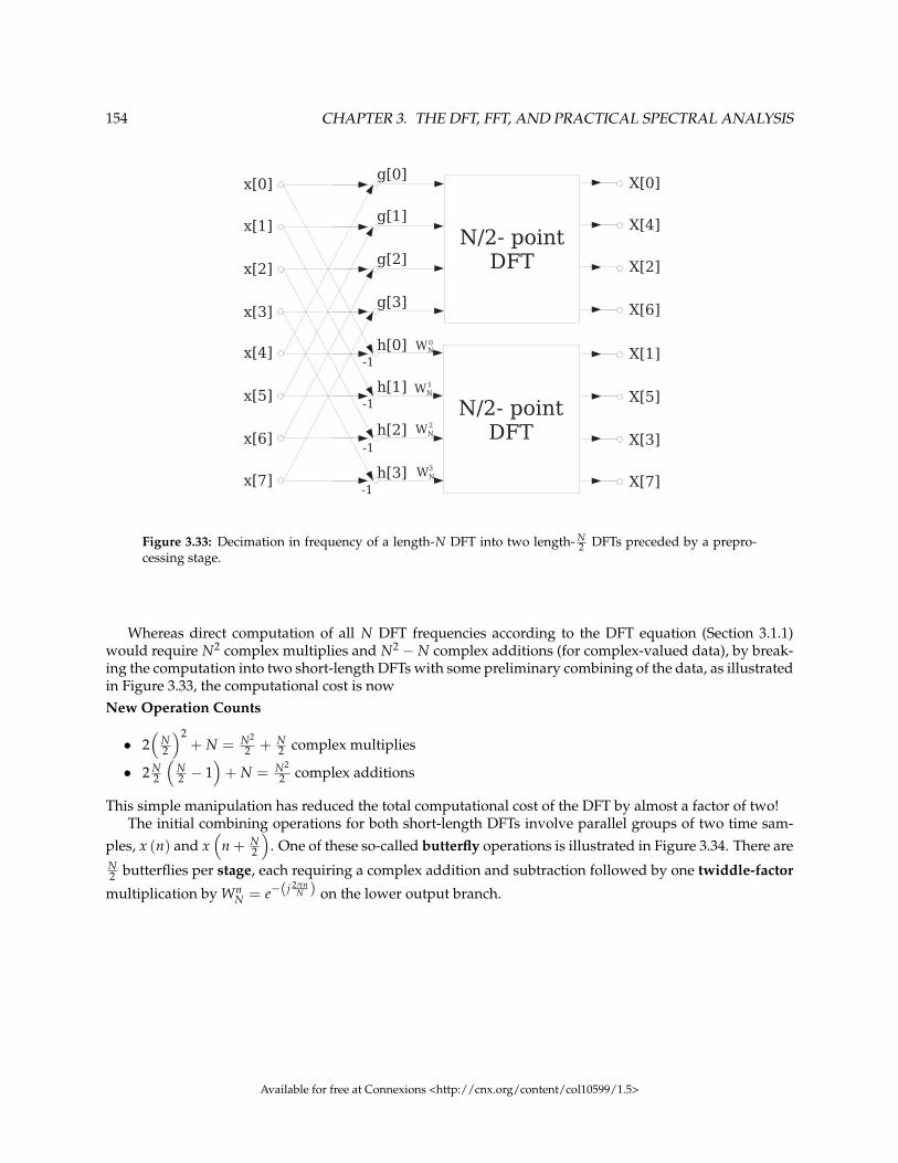
154 CHAPTER 3. THE DFT, FFT, AND PRACTICAL SPECTRAL ANALYSIS
Figure 3.33: Decimation in frequency of a length-N DFT into two length- N2 DFTs preceded by a prepro-
cessing stage.
Whereas direct computation of all N DFT frequencies according to the DFT equation (Section 3.1.1)would require N2 complex multiplies and N2 − N complex additions (for complex-valued data), by break-ing the computation into two short-length DFTs with some preliminary combining of the data, as illustratedin Figure 3.33, the computational cost is nowNew Operation Counts
• 2(
N2
)2+ N = N2
2 + N2 complex multiplies
• 2 N2
(N2 − 1
)+ N = N2
2 complex additions
This simple manipulation has reduced the total computational cost of the DFT by almost a factor of two!The initial combining operations for both short-length DFTs involve parallel groups of two time sam-
ples, x (n) and x(
n + N2
). One of these so-called butterfly operations is illustrated in Figure 3.34. There are
N2 butterflies per stage, each requiring a complex addition and subtraction followed by one twiddle-factor
multiplication by WnN = e−(j 2πn
N ) on the lower output branch.
Available for free at Connexions <http://cnx.org/content/col10599/1.5>

155
Figure 3.34: DIF butterfly: twiddle factor after length-2 DFT
It is worthwhile to note that the initial add/subtract part of the DIF butterfly is actually a length-2DFT! The theory of multi-dimensional index maps32 shows that this must be the case, and that FFTs of anyfactorable length may consist of successive stages of shorter-length FFTs with twiddle-factor multiplicationsin between. It is also worth noting that this butterfly differs from the decimation-in-time radix-2 butterfly(Figure 3.31) in that the twiddle factor multiplication occurs after the combining.
3.3.4.2.2.2 Radix-2 decimation-in-frequency algorithm
The same radix-2 decimation in frequency can be applied recursively to the two length- N2 DFT (Sec-
tion 3.1.1)s to save additional computation. When successively applied until the shorter and shorter DFTsreach length-2, the result is the radix-2 decimation-in-frequency FFT algorithm (Figure 3.35).
32"Multidimensional Index Maps" <http://cnx.org/content/m12025/latest/>
Available for free at Connexions <http://cnx.org/content/col10599/1.5>

156 CHAPTER 3. THE DFT, FFT, AND PRACTICAL SPECTRAL ANALYSIS
Figure 3.35: Radix-2 decimation-in-frequency FFT for a length-8 signal
The full radix-2 decimation-in-frequency decomposition illustrated in Figure 3.35 requires M = log2Nstages, each with N
2 butterflies per stage. Each butterfly requires 1 complex multiply and 2 adds per butter-fly. The total cost of the algorithm is thusComputational cost of radix-2 DIF FFT
• N2 log2N complex multiplies
• Nlog2N complex adds
This is a remarkable savings over direct computation of the DFT. For example, a length-1024 DFT wouldrequire 1048576 complex multiplications and 1047552 complex additions with direct computation, but only5120 complex multiplications and 10240 complex additions using the radix-2 FFT, a savings by a factor of100 or more. The relative savings increase with longer FFT lengths, and are less for shorter lengths. Mod-est additional reductions in computation can be achieved by noting that certain twiddle factors, namely
W0N , W
N2
N , WN4
N , WN8
N , W3N8
N , require no multiplications, or fewer real multiplies than other ones. By imple-menting special butterflies for these twiddle factors as discussed in FFT algorithm and programming tricks(Section 3.3.5), the computational cost of the radix-2 decimation-in-frequency FFT can be reduced to
• 2Nlog2N − 7N + 12 real multiplies• 3Nlog2N − 3N + 4 real additions
The decimation-in-frequency FFT is a flow-graph reversal of the decimation-in-time (Section 3.3.4.2.1) FFT:it has the same twiddle factors (in reverse pattern) and the same operation counts.
NOTE: In a decimation-in-frequency radix-2 FFT as illustrated in Figure 3.35, the output is inbit-reversed order (hence "decimation-in-frequency"). That is, if the frequency-sample index n iswritten as a binary number, the order is that binary number reversed. The bit-reversal process isillustrated here (Example 3.3: N=8).
Available for free at Connexions <http://cnx.org/content/col10599/1.5>

157
It is important to note that, if the input data are in order before beginning the FFT computations, the outputsof each butterfly throughout the computation can be placed in the same memory locations from which theinputs were fetched, resulting in an in-place algorithm that requires no extra memory to perform the FFT.Most FFT implementations are in-place, and overwrite the input data with the intermediate values andfinally the output.
3.3.4.2.3 Alternate FFT Structures33
Bit-reversing (Section 3.3.4.2.1) the input in decimation-in-time (DIT) FFTs (Section 3.3.4.2.1) or the outputin decimation-in-frequency (DIF) FFTs (Section 3.3.4.2.2) can sometimes be inconvenient or inefficient. Forsuch situations, alternate FFT structures have been developed. Such structures involve the same mathemat-ical computations as the standard algorithms, but alter the memory locations in which intermediate valuesare stored or the order of computation of the FFT butterflies (Section 3.3.4.2.1).
The structure in Figure 3.36 computes a decimation-in-frequency FFT (Section 3.3.4.2.2), but remapsthe memory usage so that the input is bit-reversed (Section 3.3.4.2.1), and the output is in-order as in theconventional decimation-in-time FFT (Section 3.3.4.2.1). This alternate structure is still considered a DIFFFT because the twiddle factors (Section 3.3.4.2.1) are applied as in the DIF FFT (Section 3.3.4.2.2). Thisstructure is useful if for some reason the DIF butterfly is preferred but it is easier to bit-reverse the input.
Figure 3.36: Decimation-in-frequency radix-2 FFT (Section 3.3.4.2.2) with bit-reversed input. This is an in-place (Section 3.3.4.2.1) algorithm in which the same memory can be reused throughout the computation.
33This content is available online at <http://cnx.org/content/m12012/1.6/>.
Available for free at Connexions <http://cnx.org/content/col10599/1.5>

158 CHAPTER 3. THE DFT, FFT, AND PRACTICAL SPECTRAL ANALYSIS
There is a similar structure for the decimation-in-time FFT (Section 3.3.4.2.1) with in-order inputs andbit-reversed frequencies. This structure can be useful for fast convolution (Section 3.4) on machines thatfavor decimation-in-time algorithms because the filter can be stored in bit-reverse order, and then the in-verse FFT returns an in-order result without ever bit-reversing any data. As discussed in Efficient FFTProgramming Tricks (Section 3.3.5), this may save several percent of the execution time.
The structure in Figure 3.37 implements a decimation-in-frequency FFT (Section 3.3.4.2.2) that has bothinput and output in order. It thus avoids the need for bit-reversing altogether. Unfortunately, it destroys thein-place (Section 3.3.4.2.1) structure somewhat, making an FFT program more complicated and requiringmore memory; on most machines the resulting cost exceeds the benefits. This structure can be computed inplace if two butterflies are computed simultaneously.
Figure 3.37: Decimation-in-frequency radix-2 FFT with in-order input and output. It can be computedin-place if two butterflies are computed simultaneously.
The structure in Figure 3.38 has a constant geometry; the connections between memory locations areidentical in each FFT stage (Section 3.3.4.2.1). Since it is not in-place and requires bit-reversal, it is inconve-nient for software implementation, but can be attractive for a highly parallel hardware implementation be-cause the connections between stages can be hardwired. An analogous structure exists that has bit-reversedinputs and in-order outputs.
Available for free at Connexions <http://cnx.org/content/col10599/1.5>

159
Figure 3.38: This constant-geometry structure has the same interconnect pattern from stage to stage. Thisstructure is sometimes useful for special hardware.
3.3.4.3 Radix-4 FFT Algorithms34
The radix-4 decimation-in-time (Section 3.3.4.2.1) and decimation-in-frequency (Section 3.3.4.2.2) fastFourier transforms (FFTs) (Section 3.3.1) gain their speed by reusing the results of smaller, intermediatecomputations to compute multiple DFT frequency outputs. The radix-4 decimation-in-time algorithm rear-ranges the discrete Fourier transform (DFT) equation (Section 3.1.1) into four parts: sums over all groups ofevery fourth discrete-time index n = [0, 4, 8, . . . , N − 4], n = [1, 5, 9, . . . , N − 3], n = [2, 6, 10, . . . , N − 2] andn = [3, 7, 11, . . . , N − 1] as in (3.19). (This works out only when the FFT length is a multiple of four.) Just asin the radix-2 decimation-in-time FFT (Section 3.3.4.2.1), further mathematical manipulation shows that thelength-N DFT can be computed as the sum of the outputs of four length- N
4 DFTs, of the even-indexed andodd-indexed discrete-time samples, respectively, where three of them are multiplied by so-called twiddle
factors WkN = e−(j 2πk
N ), W2kN , and W3k
N .
34This content is available online at <http://cnx.org/content/m12027/1.4/>.
Available for free at Connexions <http://cnx.org/content/col10599/1.5>

160 CHAPTER 3. THE DFT, FFT, AND PRACTICAL SPECTRAL ANALYSIS
X (k) = ∑N−1n=0 x (n) e−(j 2πnk
N ) = ∑N4 −1
n=0 x (4n) e−(
j 2π×(4n)kN
)+
∑N4 −1
n=0 x (4n + 1) e−(
j 2π(4n+1)kN
)+ ∑
N4 −1
n=0 x (4n + 2) e−(
j 2π(4n+2)kN
)+
∑N4 −1
n=0 x (4n + 3) e−(
j 2π(4n+3)kN
)= DFT N
4[x (4n)] + Wk
NDFT N4
[x (4n + 1)] +
W2kN DFT N
4[x (4n + 2)] + W3k
N DFT N4
[x (4n + 3)]
(3.19)
This is called a decimation in time because the time samples are rearranged in alternating groups, and aradix-4 algorithm because there are four groups. Figure 3.39 (Radix-4 DIT structure) graphically illustratesthis form of the DFT computation.
Available for free at Connexions <http://cnx.org/content/col10599/1.5>

161
Radix-4 DIT structure
Figure 3.39: Decimation in time of a length-N DFT into four length- N4 DFTs followed by a combining stage.
Due to the periodicity with N4 of the short-length DFTs, their outputs for frequency-sample k are reused
Available for free at Connexions <http://cnx.org/content/col10599/1.5>

162 CHAPTER 3. THE DFT, FFT, AND PRACTICAL SPECTRAL ANALYSIS
to compute X (k), X(
k + N4
), X(
k + N2
), and X
(k + 3N
4
). It is this reuse that gives the radix-4 FFT its effi-
ciency. The computations involved with each group of four frequency samples constitute the radix-4 butter-fly, which is shown in Figure 3.40. Through further rearrangement, it can be shown that this computationcan be simplified to three twiddle-factor multiplies and a length-4 DFT! The theory of multi-dimensionalindex maps35 shows that this must be the case, and that FFTs of any factorable length may consist of suc-cessive stages of shorter-length FFTs with twiddle-factor multiplications in between. The length-4 DFTrequires no multiplies and only eight complex additions (this efficient computation can be derived using aradix-2 FFT (Section 3.3.4.2.1)).
(a) (b)
Figure 3.40: The radix-4 DIT butterfly can be simplified to a length-4 DFT preceded by three twiddle-factormultiplies.
If the FFT length N = 4M, the shorter-length DFTs can be further decomposed recursively in the samemanner to produce the full radix-4 decimation-in-time FFT. As in the radix-2 decimation-in-time FFT (Sec-tion 3.3.4.2.1), each stage of decomposition creates additional savings in computation. To determine thetotal computational cost of the radix-4 FFT, note that there are M = log4N = log2 N
2 stages, each with N4
butterflies per stage. Each radix-4 butterfly requires 3 complex multiplies and 8 complex additions. Thetotal cost is thenRadix-4 FFT Operation Counts
• 3 N4
log2 N2 = 3
8 Nlog2N complex multiplies (75% of a radix-2 FFT)
• 8 N4
log2 N2 = Nlog2N complex adds (same as a radix-2 FFT)
The radix-4 FFT requires only 75% as many complex multiplies as the radix-2 (Section 3.3.4.2.1) FFTs, al-though it uses the same number of complex additions. These additional savings make it a widely-used FFTalgorithm.
The decimation-in-time operation regroups the input samples at each successive stage of decomposition,resulting in a "digit-reversed" input order. That is, if the time-sample index n is written as a base-4 number,the order is that base-4 number reversed. The digit-reversal process is illustrated for a length-N = 64example below.
Example 3.4: N = 64 = 4^3
35"Multidimensional Index Maps" <http://cnx.org/content/m12025/latest/>
Available for free at Connexions <http://cnx.org/content/col10599/1.5>

163
Original Number Original Digit Order Reversed Digit Order Digit-Reversed Number
0 000 000 0
1 001 100 16
2 002 200 32
3 003 300 48
4 010 010 4
5 011 110 20...
......
...
Table 3.2
It is important to note that, if the input signal data are placed in digit-reversed order before beginning theFFT computations, the outputs of each butterfly throughout the computation can be placed in the samememory locations from which the inputs were fetched, resulting in an in-place algorithm that requiresno extra memory to perform the FFT. Most FFT implementations are in-place, and overwrite the inputdata with the intermediate values and finally the output. A slight rearrangement within the radix-4 FFTintroduced by Burrus[4] allows the inputs to be arranged in bit-reversed (Section 3.3.4.2.1) rather thandigit-reversed order.
A radix-4 decimation-in-frequency (Section 3.3.4.2.2) FFT can be derived similarly to the radix-2 DIF FFT(Section 3.3.4.2.2), by separately computing all four groups of every fourth output frequency sample. TheDIF radix-4 FFT is a flow-graph reversal of the DIT radix-4 FFT, with the same operation counts and twiddlefactors in the reversed order. The output ends up in digit-reversed order for an in-place DIF algorithm.
Exercise 3.3.4.3.1 (Solution on p. 184.)How do we derive a radix-4 algorithm when N = 4M2?
3.3.4.4 Split-radix FFT Algorithms36
The split-radix algorithm, first clearly described and named by Duhamel and Hollman[10] in 1984, requiredfewer total multiply and add operations operations than any previous power-of-two algorithm. (Yavne[26]first derived essentially the same algorithm in 1968, but the description was so atypical that the work waslargely neglected.) For a time many FFT experts thought it to be optimal in terms of total complexity, buteven more efficient variations have more recently been discovered by Johnson and Frigo[18].
The split-radix algorithm can be derived by careful examination of the radix-2 (Section 3.3.4.2.1) andradix-4 (Section 3.3.4.3) flowgraphs as in Figure 1 below. While in most places the radix-4 (Section 3.3.4.3)algorithm has fewer nontrivial twiddle factors, in some places the radix-2 (Section 3.3.4.2.1) actually lackstwiddle factors present in the radix-4 (Section 3.3.4.3) structure or those twiddle factors simplify to multi-plication by −j, which actually requires only additions. By mixing radix-2 (Section 3.3.4.2.1) and radix-4(Section 3.3.4.3) computations appropriately, an algorithm of lower complexity than either can be derived.
36This content is available online at <http://cnx.org/content/m12031/1.5/>.
Available for free at Connexions <http://cnx.org/content/col10599/1.5>

164 CHAPTER 3. THE DFT, FFT, AND PRACTICAL SPECTRAL ANALYSIS
Motivation for split-radix algorithm
(a) radix-2 (b) radix-4
Figure 3.41: See Decimation-in-Time (DIT) Radix-2 FFT (Section 3.3.4.2.1) and Radix-4 FFT Algorithms(Section 3.3.4.3) for more information on these algorithms.
An alternative derivation notes that radix-2 butterflies of the form shown in Figure 2 can merge twiddlefactors from two successive stages to eliminate one-third of them; hence, the split-radix algorithm requiresonly about two-thirds as many multiplications as a radix-2 FFT.
(a) (b)
Figure 3.42: Note that these two butterflies are equivalent
Available for free at Connexions <http://cnx.org/content/col10599/1.5>

165
The split-radix algorithm can also be derived by mixing the radix-2 (Section 3.3.4.2.1) and radix-4 (Sec-tion 3.3.4.3) decompositions.DIT Split-radix derivation
X (k) = ∑N2 −1
n=0 x (2n) e−(
j 2π×(2n)kN
)+ ∑
N4 −1
n=0 x (4n + 1) e−(
j 2π(4n+1)kN
)+
∑N4 −1
n=0 x (4n + 3) e−(
j 2π(4n+3)kN
)= DFT N
2[x (2n)] + Wk
NDFT N4
(x (4n + 1)) +
W3kN DFT N
4(x (4n + 3))
(3.20)
Figure 3 illustrates the resulting split-radix butterfly.
Decimation-in-Time Split-Radix Butterfly
Figure 3.43: The split-radix butterfly mixes radix-2 and radix-4 decompositions and is L-shaped
Further decomposition of the half- and quarter-length DFTs yields the full split-radix algorithm. Themix of different-length FFTs in different parts of the flowgraph results in a somewhat irregular algorithm;Sorensen et al.[15] show how to adjust the computation such that the data retains the simpler radix-2 bit-reverse order. A decimation-in-frequency split-radix FFT can be derived analogously.
Available for free at Connexions <http://cnx.org/content/col10599/1.5>

166 CHAPTER 3. THE DFT, FFT, AND PRACTICAL SPECTRAL ANALYSIS
Figure 3.44: The split-radix transform has L-shaped butterflies
The multiplicative complexity of the split-radix algorithm is only about two-thirds that of the radix-2FFT, and is better than the radix-4 FFT or any higher power-of-two radix as well. The additions within thecomplex twiddle-factor multiplies are similarly reduced, but since the underlying butterfly tree remains thesame in all power-of-two algorithms, the butterfly additions remain the same and the overall reduction inadditions is much less.
Operation Counts
Complex M/As Real M/As (4/2) Real M/As (3/3)
Multiplies O[
N3 log2N
]43 Nlog2N − 38
9 N + 6 + 29 (−1)M Nlog2N − 3N + 4
Additions O [Nlog2N] 83 Nlog2N − 16
9 N + 2 + 29 (−1)M 3Nlog2N − 3N + 4
Table 3.3
Available for free at Connexions <http://cnx.org/content/col10599/1.5>

167
Comments
• The split-radix algorithm has a somewhat irregular structure. Successful progams have been written(Sorensen[15]) for uni-processor machines, but it may be difficult to efficiently code the split-radixalgorithm for vector or multi-processor machines.
• G. Bruun’s algorithm[2] requires only N − 2 more operations than the split-radix algorithm and hasa regular structure, so it might be better for multi-processor or special-purpose hardware.
• The execution time of FFT programs generally depends more on compiler- or hardware-friendly soft-ware design than on the exact computational complexity. See Efficient FFT Algorithm and Program-ming Tricks (Section 3.3.5) for further pointers and links to good code.
3.3.5 Efficient FFT Algorithm and Programming Tricks37
The use of FFT algorithms (Section 3.3.1) such as the radix-2 decimation-in-time (Section 3.3.4.2.1) ordecimation-in-frequency (Section 3.3.4.2.2) methods result in tremendous savings in computations whencomputing the discrete Fourier transform (Section 3.1.1). While most of the speed-up of FFTs comes fromthis, careful implementation can provide additional savings ranging from a few percent to several-foldincreases in program speed.
3.3.5.1 Precompute twiddle factors
The twiddle factor (Section 3.3.4.2.1), or WkN = e−(j 2πk
N ), terms that multiply the intermediate data in theFFT algorithms (Section 3.3.1) consist of cosines and sines that each take the equivalent of several multipliesto compute. However, at most N unique twiddle factors can appear in any FFT or DFT algorithm. (Forexample, in the radix-2 decimation-in-time FFT (Section 3.3.4.2.1), only N
2 twiddle factors WNk , k =
0, 1, 2, . . . , N2 − 1
are used.) These twiddle factors can be precomputed once and stored in an array in
computer memory, and accessed in the FFT algorithm by table lookup. This simple technique yields verysubstantial savings and is almost always used in practice.
3.3.5.2 Compiler-friendly programming
On most computers, only some of the total computation time of an FFT is spent performing the FFT but-terfly computations; determining indices, loading and storing data, computing loop parameters and otheroperations consume the majority of cycles. Careful programming that allows the compiler to generate ef-ficient code can make a several-fold improvement in the run-time of an FFT. The best choice of radix interms of program speed may depend more on characteristics of the hardware (such as the number of CPUregisters) or compiler than on the exact number of computations. Very often the manufacturer’s librarycodes are carefully crafted by experts who know intimately both the hardware and compiler architectureand how to get the most performance out of them, so use of well-written FFT libraries is generally rec-ommended. Certain freely available programs and libraries are also very good. Perhaps the best currentgeneral-purpose library is the FFTW38 package; information can be found at http://www.fftw.org39 . Apaper by Frigo and Johnson[12] describes many of the key issues in developing compiler-friendly code.
3.3.5.3 Program in assembly language
While compilers continue to improve, FFT programs written directly in the assembly language of a spe-cific machine are often several times faster than the best compiled code. This is particularly true for DSPmicroprocessors, which have special instructions for accelerating FFTs that compilers don’t use. (I have
37This content is available online at <http://cnx.org/content/m12021/1.6/>.38http://www.fftw.org39http://www.fftw.org
Available for free at Connexions <http://cnx.org/content/col10599/1.5>

168 CHAPTER 3. THE DFT, FFT, AND PRACTICAL SPECTRAL ANALYSIS
myself seen differences of up to 26 to 1 in favor of assembly!) Very often, FFTs in the manufacturer’sor high-performance third-party libraries are hand-coded in assembly. For DSP microprocessors, the codesdeveloped by Meyer, Schuessler, and Schwarz[19] are perhaps the best ever developed; while the particularprocessors are now obsolete, the techniques remain equally relevant today. Most DSP processors providespecial instructions and a hardware design favoring the radix-2 decimation-in-time algorithm, which isthus generally fastest on these machines.
3.3.5.4 Special hardware
Some processors have special hardware accelerators or co-processors specifically designed to accelerateFFT computations. For example, AMI Semiconductor’s40 Toccata41 ultra-low-power DSP microprocessorfamily, which is widely used in digital hearing aids, have on-chip FFT accelerators; it is always faster andmore power-efficient to use such accelerators and whatever radix they prefer.
In a surprising number of applications, almost all of the computations are FFTs. A number of special-purpose chips are designed to specifically compute FFTs, and are used in specialized high-performanceapplications such as radar systems. Other systems, such as OFDM42 -based communications receivers,have special FFT hardware built into the digital receiver circuit. Such hardware can run many times faster,with much less power consumption, than FFT programs on general-purpose processors.
3.3.5.5 Effective memory management
Cache misses or excessive data movement between registers and memory can greatly slow down an FFTcomputation. Efficient programs such as the FFTW package43 are carefully designed to minimize these in-efficiences. In-place algorithms (Section 3.3.4.2.1) reuse the data memory throughout the transform, whichcan reduce cache misses for longer lengths.
3.3.5.6 Real-valued FFTs
FFTs of real-valued signals require only half as many computations as with complex-valued data. There areseveral methods for reducing the computation, which are described in more detail in Sorensen et al.[16]
1. Use DFT symmetry properties (Section 3.1.1) to do two real-valued DFTs at once with one FFT pro-gram
2. Perform one stage of the radix-2 decimation-in-time (Section 3.3.4.2.1) decomposition and computethe two length- N
2 DFTs using the above approach.3. Use a direct real-valued FFT algorithm; see H.V. Sorensen et.al.[16]
3.3.5.7 Special cases
Occasionally only certain DFT frequencies are needed, the input signal values are mostly zero, the signalis real-valued (as discussed above), or other special conditions exist for which faster algorithms can bedeveloped. Sorensen and Burrus[22] describe slightly faster algorithms for pruned44 or zero-padded (Sec-tion 3.2.1.5: Zero-Padding) data. Goertzel’s algorithm (Section 3.3.3) is useful when only a few DFT outputsare needed. The running FFT (Section 3.3.2) can be faster when DFTs of highly overlapped blocks of dataare needed, as in a spectrogram (Section 3.2.3).
40http://www.amis.com41http://www.amis.com/products/dsp/toccata_plus.html42http://en.wikipedia.org/wiki/OFDM43http://www.fftw.org44http://www.fftw.org/pruned.html
Available for free at Connexions <http://cnx.org/content/col10599/1.5>

169
3.3.5.8 Higher-radix algorithms
Higher-radix algorithms, such as the radix-4 (Section 3.3.4.3), radix-8, or split-radix (Section 3.3.4.4) FFTs,require fewer computations and can produce modest but worthwhile savings. Even the split-radix FFT(Section 3.3.4.4) reduces the multiplications by only 33% and the additions by a much lesser amount relativeto the radix-2 FFTs (Section 3.3.4.2.1); significant improvements in program speed are often due to implicitloop-unrolling45 or other compiler benefits than from the computational reduction itself!
3.3.5.9 Fast bit-reversal
Bit-reversing (Section 3.3.4.2.1) the input or output data can consume several percent of the total run-timeof an FFT program. Several fast bit-reversal algorithms have been developed that can reduce this to twopercent or less, including the method published by D.M.W. Evans[11].
3.3.5.10 Trade additions for multiplications
When FFTs first became widely used, hardware multipliers were relatively rare on digital computers, andmultiplications generally required many more cycles than additions. Methods to reduce multiplications,even at the expense of a substantial increase in additions, were often beneficial. The prime factor algo-rithms46 and the Winograd Fourier transform algorithms (Section 3.6), which required fewer multipliesand considerably more additions than the power-of-two-length algorithms (Section 3.3.4.1), were devel-oped during this period. Current processors generally have high-speed pipelined hardware multipliers,so trading multiplies for additions is often no longer beneficial. In particular, most machines now supportsingle-cycle multiply-accumulate (MAC) operations, so balancing the number of multiplies and adds andcombining them into single-cycle MACs generally results in the fastest code. Thus, the prime-factor andWinograd FFTs are rarely used today unless the application requires FFTs of a specific length.
It is possible to implement a complex multiply with 3 real multiplies and 5 real adds rather than theusual 4 real multiplies and 2 real adds:
(C + jS) (X + jY) = CX− SY + j (CY + SX)
but alernativelyZ = C (X−Y)
D = C + S
E = C− S
CX− SY = EY + Z
CY + SX = DX− Z
In an FFT, D and E come entirely from the twiddle factors, so they can be precomputed and stored in alook-up table. This reduces the cost of the complex twiddle-factor multiply to 3 real multiplies and 3 realadds, or one less and one more, respectively, than the conventional 4/2 computation.
45http://en.wikipedia.org/wiki/Loop_unrolling46"The Prime Factor Algorithm" <http://cnx.org/content/m12033/latest/>
Available for free at Connexions <http://cnx.org/content/col10599/1.5>

170 CHAPTER 3. THE DFT, FFT, AND PRACTICAL SPECTRAL ANALYSIS
3.3.5.11 Special butterflies
Certain twiddle factors, namely W0N = 1, W
N2
N , WN4
N , WN8
N , W3N8
N , etc., can be implemented with no additionaloperations, or with fewer real operations than a general complex multiply. Programs that specially imple-ment such butterflies in the most efficient manner throughout the algorithm can reduce the computationalcost by up to several N multiplies and additions in a length-N FFT.
3.3.5.12 Practical Perspective
When optimizing FFTs for speed, it can be important to maintain perspective on the benefits that can beexpected from any given optimization. The following list categorizes the various techniques by potentialbenefit; these will be somewhat situation- and machine-dependent, but clearly one should begin with themost significant and put the most effort where the pay-off is likely to be largest.Methods to speed up computation of DFTs
• Tremendous Savings -
a. FFT ( Nlog2 N savings)
• Substantial Savings - (2)
a. Table lookup of cosine/sineb. Compiler tricks/good programmingc. Assembly-language programmingd. Special-purpose hardwaree. Real-data FFT for real data (factor of 2)f. Special cases
• Minor Savings -
a. radix-4 (Section 3.3.4.3), split-radix (Section 3.3.4.4) (-10% - +30%)b. special butterfliesc. 3-real-multiplication complex multiplyd. Fast bit-reversal (up to 6%)
NOTE: On general-purpose machines, computation is only part of the total run time. Addressgeneration, indexing, data shuffling, and memory access take up much or most of the cycles.
NOTE: A well-written radix-2 (Section 3.3.4.2.1) program will run much faster than a poorly writ-ten split-radix (Section 3.3.4.4) program!
3.4 Fast Convolution47
3.4.1 Fast Circular Convolution
Since,N−1
∑m=0
x (m) h (n−m) modN = y (n) is equivalent toY (k) = X (k) H (k)
y (n) can be computed as y (n) = IDFT [DFT [x (n)] DFT [h (n)]]Cost
• Direct47This content is available online at <http://cnx.org/content/m12022/1.5/>.
• Available for free at Connexions <http://cnx.org/content/col10599/1.5>

171
· N2 complex multiplies.· N (N − 1) complex adds.
Via FFTs
· 3 FFTs + N multipies.· N + 3N
2 log2N complex multiplies.· 3 (Nlog2N) complex adds.
If H (k) can be precomputed, cost is only 2 FFts + N multiplies.
3.4.2 Fast Linear Convolution
DFT (3.5) produces cicular convolution. For linear convolution, we must zero-pad sequences so that circularwrap-around always wraps over zeros.
Figure 3.45
To achieve linear convolution using fast circular convolution, we must use zero-padded DFTs of lengthN ≥ L + M− 1
Available for free at Connexions <http://cnx.org/content/col10599/1.5>

172 CHAPTER 3. THE DFT, FFT, AND PRACTICAL SPECTRAL ANALYSIS
Figure 3.46
Choose shortest convenient N (usually smallest power-of-two greater than or equal to L + M− 1)
y (n) = IDFTN [DFTN [x (n)] DFTN [h (n)]]
NOTE: There is some inefficiency when compared to circular convolution due to longer zero-padded DFTs (3.5). Still, O
(N
log2 N
)savings over direct computation.
3.4.3 Running Convolution
Suppose L = ∞, as in a real time filter application, or L M. There are efficient block methods forcomputing fast convolution.
3.4.3.1 Overlap-Save (OLS) Method
Note that if a length-M filter h (n) is circularly convulved with a length-N segment of a signal x (n),
Available for free at Connexions <http://cnx.org/content/col10599/1.5>

173
Figure 3.47
the first M− 1 samples are wrapped around and thus is incorrect. However, for M− 1 ≤ n ≤ N− 1,theconvolution is linear convolution, so these samples are correct. Thus N−M + 1 good outputs are producedfor each length-N circular convolution.
The Overlap-Save Method: Break long signal into successive blocks of N samples, each block overlap-ping the previous block by M − 1 samples. Perform circular convolution of each block with filter h (m).Discard first M− 1 points in each output block, and concatenate the remaining points to create y (n).
Available for free at Connexions <http://cnx.org/content/col10599/1.5>

174 CHAPTER 3. THE DFT, FFT, AND PRACTICAL SPECTRAL ANALYSIS
Figure 3.48
Computation cost for a length-N equals 2n FFT per output sample is (assuming precomputed H (k)) 2FFTs and N multiplies
2(
N2 log2N
)+ N
N −M + 1=
N (log2N + 1)N −M + 1
complex multiplies
Available for free at Connexions <http://cnx.org/content/col10599/1.5>

175
2 (Nlog2N)N −M + 1
=2Nlog2N
N −M + 1complex adds
Compare to M mults, M− 1 adds per output point for direct method. For a given M, optimal N can bedetermined by finding N minimizing operation counts. Usualy, optimal N is 4M ≤ Nopt ≤ 8M.
3.4.3.2 Overlap-Add (OLA) Method
Zero-pad length-L blocks by M− 1 samples.
Figure 3.49
Add successive blocks, overlapped by M − 1 samples, so that the tails sum to produce the completelinear convolution.
Available for free at Connexions <http://cnx.org/content/col10599/1.5>

176 CHAPTER 3. THE DFT, FFT, AND PRACTICAL SPECTRAL ANALYSIS
Figure 3.50
Computational Cost: Two length N = L + M− 1 FFTs and M mults and M− 1 adds per L output points;essentially the sames as OLS method.
Available for free at Connexions <http://cnx.org/content/col10599/1.5>

177
3.5 Chirp-z Transform48
Let zk = AW−k, where A = Aoejθo , W = Woe−(jφo).We wish to compute M samples, k = [0, 1, 2, . . . , M− 1] of
X (zk) =N−1
∑n=0
x (n) zk−n =
N−1
∑n=0
x (n) A−nWnk
Figure 3.51
48This content is available online at <http://cnx.org/content/m12013/1.4/>.
Available for free at Connexions <http://cnx.org/content/col10599/1.5>

178 CHAPTER 3. THE DFT, FFT, AND PRACTICAL SPECTRAL ANALYSIS
Note that((k− n)2 = n2 − 2nk + k2
)⇒(
nk = 12
(n2 + k2 − (k− n)2
)), So
X (zk) =N−1
∑n=0
x (n) A−nWn22 W
k22 W
−(k−n)22
Wk22
N−1
∑n=0
x (n) A−nWn22 W
−(k−n)22
Thus, X (zk) can be compared by
1. Premultiply x (n) by AnWn22 , n = [0, 1, . . . , N − 1] to make y (n)
2. Linearly convolve with W−(k−n)2
2
3. Post multiply by to get Wk22 to get X (zk).
1. (list, item 1, p. 178) and 3. (list, item 3, p. 178) require N and M operations respectively. 2. (list, item 2,p. 178) can be performed efficiently using fast convolution.
Figure 3.52
W−n22 is required only for − (N − 1) ≤ n ≤ M− 1, so this linear convolution can be implemented with
L ≥ N + M− 1 FFTs.
NOTE: Wrap W−n22 around L when implementing with circular convolution.
So, a weird-length DFT can be implemented relatively efficiently using power-of-two algorithms via thechirp-z transform.
Also useful for "zoom-FFTs".
Available for free at Connexions <http://cnx.org/content/col10599/1.5>

179
3.6 FFTs of prime length and Rader’s conversion49
The power-of-two FFT algorithms (Section 3.3.4.1), such as the radix-2 (Section 3.3.4.2.1) and radix-4 (Sec-tion 3.3.4.3) FFTs, and the common-factor50 and prime-factor51 FFTs, achieve great reductions in compu-tational complexity of the DFT (Section 3.1.1) when the length, N, is a composite number. DFTs of primelength are sometimes needed, however, particularly for the short-length DFTs in common-factor or prime-factor algorithms. The methods described here, along with the composite-length algorithms, allow fastcomputation of DFTs of any length.
There are two main ways of performing DFTs of prime length:
1. Rader’s conversion, which is most efficient, and the2. Chirp-z transform (Section 3.5), which is simpler and more general.
Oddly enough, both work by turning prime-length DFTs into convolution! The resulting convolutions canthen be computed efficiently by either
1. fast convolution (Section 3.4) via composite-length FFTs (simpler) or by2. Winograd techniques (more efficient)
3.6.1 Rader’s Conversion
Rader’s conversion is a one-dimensional index-mapping52 scheme that turns a length-N DFT (3.5) (Nprime) into a length-( N − 1) convolution and a few additions. Rader’s conversion works only for prime-length N.
An index map simply rearranges the order of the sum operation in the DFT definition (Section 3.1.1).Because addition is a commutative operation, the same mathematical result is produced from any order, aslong as all of the same terms are added once and only once. (This is the condition that defines an indexmap.) Unlike the multi-dimensional index maps53 used in deriving common factor54 and prime-factorFFTs55, Rader’s conversion uses a one-dimensional index map in a finite group of N integers: k = rmmodN
3.6.1.1 Fact from number theory
If N is prime, there exists an integer "r" called a primitive root, such that the index map k = rmmodN,m = [0, 1, 2, . . . , N − 2], uniquely generates all elements k = [1, 2, 3, . . . , N − 1]
Example 3.5N = 5, r = 2
20mod5 = 1
21mod5 = 2
22mod5 = 4
23mod5 = 3
49This content is available online at <http://cnx.org/content/m12023/1.3/>.50"Multidimensional Index Maps" <http://cnx.org/content/m12025/latest/>51"The Prime Factor Algorithm" <http://cnx.org/content/m12033/latest/>52"Multidimensional Index Maps" <http://cnx.org/content/m12025/latest/>53"Multidimensional Index Maps" <http://cnx.org/content/m12025/latest/>54"Multidimensional Index Maps" <http://cnx.org/content/m12025/latest/>55"The Prime Factor Algorithm" <http://cnx.org/content/m12033/latest/>
Available for free at Connexions <http://cnx.org/content/col10599/1.5>

180 CHAPTER 3. THE DFT, FFT, AND PRACTICAL SPECTRAL ANALYSIS
3.6.1.2 Another fact from number theory
For N prime, the inverse of r (i.e. r−1rmodN = 1 is also a primitive root (call it r−1).
Example 3.6N = 5, r = 2 r−1 = 3
2× 3mod5 = 1
30mod5 = 1
31mod5 = 3
32mod5 = 4
33mod5 = 2
So why do we care? Because we can use these facts to turn a DFT (3.5) into a convolution!
3.6.1.3 Rader’s Conversion
Let n = r−mmodN , (m = [0, 1, . . . , N − 2]) ∧ n ∈ [1, 2, . . . , N − 1] , k =rpmodN , (p = [0, 1, . . . , N − 2]) ∧ k ∈ [1, 2, . . . , N − 1]
X (k) =N−1
∑n=0
x (n) WnkN =
x (0) + ∑N−1n=1 x (n) Wnk
N if k 6= 0
∑N−1n=0 x (n) if k = 0
where for convenience WnkN = e−(j 2πnk
N ) in the DFT equation. For k 6= 0
X (rpmodN) = ∑N−2m=0 x (r−mmodN) Wrpr−m
+ x (0)
= ∑N−2m=0 x (r−mmodN) Wrp−m
+ x (0)
= x (0) + x(
r−lmodN)∗Wrl
(3.21)
where l = [0, 1, . . . , N − 2]
Example 3.7N = 5, r = 2, r−1 = 3
X (0)
X (1)
X (2)
X (3)
X (4)
=
0 0 0 0 0
0 1 2 3 4
0 2 4 1 3
0 3 1 4 2
0 4 3 2 1
x (0)
x (1)
x (2)
x (3)
x (4)
X (0)
X (1)
X (2)
X (4)
X (3)
=
0 0 0 0 0
0 1 3 4 2
0 2 1 3 4
0 4 2 1 1
0 3 4 2 3
x (0)
x (1)
x (3)
x (4)
x (2)
Available for free at Connexions <http://cnx.org/content/col10599/1.5>

181
where for visibility the matrix entries represent only the power, m of the corresponding DFT termWm
N Note that the 4-by-4 circulant matrix56
1 3 4 2
2 1 3 4
4 2 1 1
3 4 2 3
corresponds to a length-4 circular convolution.
Rader’s conversion turns a prime-length DFT (3.5) into a few adds and a composite-length (N− 1) circularconvolution, which can be computed efficiently using either
1. fast convolution (Section 3.4) via FFT and IFFT2. index-mapped convolution algorithms and short Winograd convolution alogrithms. (Rather compli-
cated, and trades fewer multiplies for many more adds, which may not be worthwile on most modernprocessors.) See R.C. Agarwal and J.W. Cooley[1]
3.6.2 Winograd minimum-multiply convolution and DFT algorithms
S. Winograd has proved that a length-N circular or linear convolution or DFT (3.5) requires less than 2Nmultiplies (for real data), or 4N real multiplies for complex data. (This doesn’t count multiplies by rationalfractions, like 3 or 1
N or 517 , which can be computed with additions and one overall scaling factor.) Fur-
thermore, Winograd showed how to construct algorithms achieving these counts. Winograd prime-lengthDFTs and convolutions have the following characteristics:
1. Extremely efficient for small N (N < 20)2. The number of adds becomes huge for large N.
Thus Winograd’s minimum-multiply FFT’s are useful only for small N. They are very important for Prime-Factor Algorithms57, which generally use Winograd modules to implement the short-length DFTs. Tablesgiving the multiplies and adds necessary to compute Winograd FFTs for various lengths can be found inC.S. Burrus (1988) [3]. Tables and FORTRAN and TMS32010 programs for these short-length transformscan be found in C.S. Burrus and T.W. Parks (1985) [5]. The theory and derivation of these algorithms isquite elegant but requires substantial background in number theory and abstract algebra. Fortunately forthe practitioner, all of the short algorithms one is likely to need have already been derived and can simplybe looked up without mastering the details of their derivation.
3.6.3 Winograd Fourier Transform Algorithm (WFTA)
The Winograd Fourier Transform Algorithm (WFTA) is a technique that recombines the short Winogradmodules in a prime-factor FFT58 into a composite-N structure with fewer multiplies but more adds. Whiletheoretically interesting, WFTAs are complicated and different for every length, and on modern processorswith hardware multipliers the trade of multiplies for many more adds is very rarely useful in practice today.
56http://en.wikipedia.org/wiki/Circulant_matrix57"The Prime Factor Algorithm" <http://cnx.org/content/m12033/latest/>58"The Prime Factor Algorithm" <http://cnx.org/content/m12033/latest/>
Available for free at Connexions <http://cnx.org/content/col10599/1.5>

182 CHAPTER 3. THE DFT, FFT, AND PRACTICAL SPECTRAL ANALYSIS
3.7 Choosing the Best FFT Algorithm59
3.7.1 Choosing an FFT length
The most commonly used FFT algorithms by far are the power-of-two-length FFT (Section 3.3.4.1) algo-rithms. The Prime Factor Algorithm (PFA)60 and Winograd Fourier Transform Algorithm (WFTA) (Sec-tion 3.6.3: Winograd Fourier Transform Algorithm (WFTA)) require somewhat fewer multiplies, but theoverall difference usually isn’t sufficient to warrant the extra difficulty. This is particularly true now thatmost processors have single-cycle pipelined hardware multipliers, so the total operation count is more rel-evant. As can be seen from the following table, for similar lengths the split-radix algorithm is comparablein total operations to the Prime Factor Algorithm, and is considerably better than the WFTA, although thePFA and WTFA require fewer multiplications and more additions. Many processors now support singlecycle multiply-accumulate (MAC) operations; in the power-of-two algorithms all multiplies can be com-bined with adds in MACs, so the number of additions is the most relevant indicator of computationalcost.
Representative FFT Operation Counts
FFT length Multiplies (real) Adds(real) Mults + Adds
Radix 2 1024 10248 30728 40976
Split Radix 1024 7172 27652 34824
Prime Factor Alg 1008 5804 29100 34904
Winograd FT Alg 1008 3548 34416 37964
Table 3.4
The Winograd Fourier Transform Algorithm (Section 3.6.3: Winograd Fourier Transform Algorithm(WFTA)) is particularly difficult to program and is rarely used in practice. For applications in which thetransform length is somewhat arbitrary (such as fast convolution or general spectrum analysis), the lengthis usually chosen to be a power of two. When a particular length is required (for example, in the USAeach carrier has exactly 416 frequency channels in each band in the AMPS61 cellular telephone standard),a Prime Factor Algorithm62 for all the relatively prime terms is preferred, with a Common Factor Algo-rithm63 for other non-prime lengths. Winograd’s short-length modules (Section 3.6) should be used forthe prime-length factors that are not powers of two. The chirp z-transform (Section 3.5) offers a univer-sal way to compute any length DFT (Section 3.2.1) (for example, Matlab64 reportedly uses this method forlengths other than a power of two), at a few times higher cost than that of a CFA or PFA optimized for thatspecific length. The chirp z-transform (Section 3.5), along with Rader’s conversion (Section 3.6.1: Rader’sConversion), assure us that algorithms of O (NlogN) complexity exist for any DFT length N.
3.7.2 Selecting a power-of-two-length algorithm
The choice of a power-of-two algorithm may not just depend on computational complexity. The latest ex-tensions of the split-radix algorithm (Section 3.3.4.4) offer the lowest known power-of-two FFT operationcounts, but the 10%-30% difference may not make up for other factors such as regularity of structure or data
59This content is available online at <http://cnx.org/content/m12060/1.3/>.60"The Prime Factor Algorithm" <http://cnx.org/content/m12033/latest/>61http://en.wikipedia.org/wiki/AMPS62"The Prime Factor Algorithm" <http://cnx.org/content/m12033/latest/>63"Multidimensional Index Maps" <http://cnx.org/content/m12025/latest/>64http://www.mathworks.com/products/matlab/
Available for free at Connexions <http://cnx.org/content/col10599/1.5>

183
flow, FFT programming tricks (Section 3.3.5), or special hardware features. For example, the decimation-in-time radix-2 FFT (Section 3.3.4.2.1) is the fastest FFT on Texas Instruments’65 TMS320C54x DSP micro-processors, because this processor family has special assembly-language instructions that accelerate thisparticular algorithm. On other hardware, radix-4 algorithms (Section 3.3.4.3) may be more efficient. Somedevices, such as AMI Semiconductor’s66 Toccata67 ultra-low-power DSP microprocessor family, have on-chip FFT accelerators; it is always faster and more power-efficient to use these accelerators and whateverradix they prefer. For fast convolution (Section 3.4), the decimation-in-frequency (Section 3.3.4.2.2) algo-rithms may be preferred because the bit-reversing can be bypassed; however, most DSP microprocessorsprovide zero-overhead bit-reversed indexing hardware and prefer decimation-in-time algorithms, so thismay not be true for such machines. Good, compiler- or hardware-friendly programming always mattersmore than modest differences in raw operation counts, so manufacturers’ or good third-party FFT librariesare often the best choice. The module FFT programming tricks (Section 3.3.5) references some good, freeFFT software (including the FFTW68 package) that is carefully coded to be compiler-friendly; such codesare likely to be considerably faster than codes written by the casual programmer.
3.7.3 Multi-dimensional FFTs
Multi-dimensional FFTs pose additional possibilities and problems. The orthogonality and separabilityof multi-dimensional DFTs allows them to be efficiently computed by a series of one-dimensional FFTsalong each dimension. (For example, a two-dimensional DFT can quickly be computed by performingFFTs of each row of the data matrix followed by FFTs of all columns, or vice-versa.) Vector-radix FFTshave been developed with higher efficiency per sample than row-column algorithms. Multi-dimensionaldatasets, however, are often large and frequently exceed the cache size of the processor, and excessive cachemisses may increase the computational time greatly, thus overwhelming any minor complexity reductionfrom a vector-radix algorithm. Either vector-radix FFTs must be carefully programmed to match the cachelimitations of a specific processor, or a row-column approach should be used with matrix transposition inbetween to ensure data locality for high cache utilization throughout the computation.
3.7.4 Few time or frequency samples
FFT algorithms gain their efficiency through intermediate computations that can be reused to computemany DFT frequency samples at once. Some applications require only a handful of frequency samples tobe computed; when that number is of order less than O (logN), direct computation of those values viaGoertzel’s algorithm (Section 3.3.3) is faster. This has the additional advantage that any frequency, not justthe equally-spaced DFT frequency samples, can be selected. Sorensen and Burrus[23] developed algorithmsfor when most input samples are zero or only a block of DFT frequencies are needed, but the computationalcost is of the same order.
Some applications, such as time-frequency analysis via the short-time Fourier transform (Section 3.2.3)or spectrogram (Section 3.2.3), require DFTs of overlapped blocks of discrete-time samples. When the step-size between blocks is less than O (logN), the running FFT (Section 3.3.2) will be most efficient. (Note thatany window must be applied via frequency-domain convolution, which is quite efficient for sinusoidalwindows such as the Hamming window.) For step-sizes of O (logN) or greater, computation of the DFT ofeach successive block via an FFT is faster.
65http://www.ti.com/66http://www.amis.com67http://www.amis.com/products/dsp/toccata_plus.html68http://www.fftw.org/
Available for free at Connexions <http://cnx.org/content/col10599/1.5>

184 CHAPTER 3. THE DFT, FFT, AND PRACTICAL SPECTRAL ANALYSIS
Solutions to Exercises in Chapter 3
Solution to Exercise 3.2.1.1 (p. 112)In general, NO. The DTFT exactly corresponds to the continuous-time Fourier transform only when the sig-nal is bandlimited and sampled at more than twice its highest frequency. The DFT frequency values exactlycorrespond to frequency samples of the DTFT only when the discrete-time signal is time-limited. However,a bandlimited continuous-time signal cannot be time-limited, so in general these conditions cannot both besatisfied.
It can, however, be true for a small class of analog signals which are not time-limited but happen toexactly equal zero at all sample times outside of the interval n ∈ [0, N − 1]. The sinc function with abandwidth equal to the Nyquist frequency and centered at t = 0 is an example.Solution to Exercise 3.2.3.1 (p. 130)
Solution to Exercise 3.2.3.2 (p. 137)
Solution to Exercise 3.2.3.3 (p. 138)
Solution to Exercise 3.3.4.3.1 (p. 163)Perform a radix-2 decomposition for one stage, then radix-4 decompositions of all subsequent shorter-
length DFTs.
Available for free at Connexions <http://cnx.org/content/col10599/1.5>

Chapter 4
Wavelets
4.1 Time Frequency Analysis and Continuous Wavelet Transform
4.1.1 Why Transforms?1
In the field of signal processing we frequently encounter the use of transforms. Transforms are named suchbecause they take a signal and transform it into another signal, hopefully one which is easier to processor analyze than the original. Essentially, transforms are used to manipulate signals such that their mostimportant characteristics are made plainly evident. To isolate a signal’s important characteristics, however,one must employ a transform that is well matched to that signal. For example, the Fourier transform, whilewell matched to certain classes of signal, does not efficiently extract information about signals in otherclasses. This latter fact motivates our development of the wavelet transform.
4.1.2 Limitations of Fourier Analysis2
Let’s consider the Continuous-Time Fourier Transform (CTFT) pair:
X (Ω) =∫ ∞
−∞x (t) e−(jΩt)dt
x (t) =1
2π
∫ ∞
−∞X (Ω) ejΩtdΩ
The Fourier transform pair supplies us with our notion of "frequency." In other words, all of our intuitionsregarding the relationship between the time domain and the frequency domain can be traced to this partic-ular transform pair.
It will be useful to view the CTFT in terms of basis elements. The inverse CTFT equation abovesays that the time-domain signal x (t) can be expressed as a weighted summation of basis elements bΩ (t) , bΩ (t) | −∞ < Ω < ∞, where bΩ (t) = ejΩt is the basis element corresponding to frequency Ω.In other words, the basis elements are parameterized by the variable Ω that we call frequency. Finally,X (Ω) specifies the weighting coefficient for bΩ (t). In the case of the CTFT, the number of basis elements isuncountably infinite, and thus we need an integral to express the summation.
The Fourier Series (FS) can be considered as a special sub-case of the CTFT that applies when the time-domain signal is periodic. Recall that if x (t) is periodic with period T, then it can be expressed as a weighted
1This content is available online at <http://cnx.org/content/m11001/2.1/>.2This content is available online at <http://cnx.org/content/m11003/2.1/>.
Available for free at Connexions <http://cnx.org/content/col10599/1.5>
185

186 CHAPTER 4. WAVELETS
summation of basis elements bk (t) |∞k=−∞, where bk (t) = ej 2πT tk:
x (t) =∞
∑k=−∞
X [k] ej 2πT tk
X [k] =1T
∫ T2
− T2
x (t) e−(j 2πT tk)dt
Here the basis elements comes from a countably-infinite set, parameterized by the frequency index k ∈ Z.The coefficients X [k] |∞k=−∞ specify the strength of the corresponding basis elements within signal x (t).
Though quite popular, Fourier analysis is not always the best tool to analyze a signal whose characteris-tics vary with time. For example, consider a signal composed of a periodic component plus a sharp "glitch"at time t0, illustrated in time- and frequency-domains, Figure 4.1.
Figure 4.1
Fourier analysis is successful in reducing the complicated-looking periodic component into a few simpleparameters: the frequencies Ω1, Ω2 and their corresponding magnitudes/phases. The glitch component,described compactly in terms of the time-domain location t0 and amplitude, however, is not describedefficiently in the frequency domain since it produces a wide spread of frequency components. Thus, neithertime- nor frequency-domain representations alone give an efficient description of the glitched periodicsignal: each representation distills only certain aspects of the signal.
As another example, consider the linear chirp x (t) = sin(Ωt2) illustrated in Figure 4.2.
Available for free at Connexions <http://cnx.org/content/col10599/1.5>

187
Figure 4.2
Though written using the sin (·) function, the chirp is not described by a single Fourier frequency. Wemight try to be clever and write
sin(
Ωt2)
= sin (Ωt · t) = sin (Ω (t) · t)
where it now seems that signal has an instantaneous frequency Ω (t) = Ωt which grows linearly in time.But here we must be cautious! Our newly-defined instantaneous frequency Ω (t) is not consistent with theFourier notion of frequency. Recall that the CTFT says that a signal can be constructed as a superposition offixed-frequency basis elements ejΩt with time support from −∞ to + (∞); these elements are evenly spreadout over all time, and so there is noting instantaneous about Fourier frequency! So, while instantaneousfrequency gives a compact description of the linear chirp, Fourier analysis is not capable of uncovering thissimple structure.
As a third example, consider a sinusoid of frequency Ω0 that is rectangularly windowed to extract onlyone period (Figure 4.3).
Figure 4.3
Instantaneous-frequency arguments would claim that
x (t) = sin (Ω (t) · t) , Ω (t) =
Ω0 if t ∈ window
0 if t /∈ window
Available for free at Connexions <http://cnx.org/content/col10599/1.5>
188 CHAPTER 4. WAVELETS
where Ω (t) takes on exactly two distinct "frequency" values. In contrast, Fourier theory says that rectan-gular windowing induces a frequency-domain spreading by a sin(Ω)
Ω profile, resulting in a continuum ofFourier frequency components. Here again we see that Fourier analysis does not efficiently decomposesignals whose "instantaneous frequency" varies with time.
4.1.3 Time-Frequency Uncertainty Principle3
Recall that Fourier basis elements bΩ (t) = ejΩt exhibit poor time localization abilities - a consequence ofthe fact that bΩ (t) is evenly spread over all t ∈ (−∞, ∞). By time localization we mean the ability toclearly identify signal events which manifest during a short time interval, such as the "glitch" described inan earlier example.
At the opposite extreme, a basis composed of shifted Dirac deltas bτ (t) = ∆ (t− τ) would have excellenttime localization but terrible "frequency localization," since every Dirac basis element is evenly spread overall Fourier frequencies Ω ∈ [−∞, ∞]. This can be seen via |Bτ (Ω) | = |
∫ ∞−∞ bτ (t) e−(jΩt)dt| = 1 ∀ (Ω),
regardless of τ. By frequency localization we mean the ability to clearly identify signal components whichare concentrated at particular Fourier frequencies, such as sinusoids.
These observations motivate the question: does there exist a basis that provides both excellent frequencylocalization and excellent time localization? The answer is "not really": there is a fundamental tradeoffbetween the time localization and frequency localization of any basis element. This idea is made concretebelow.
Let us consider an arbitrary waveform, or basis element, b (t). Its CTFT will be denoted by B (Ω). Definethe energy of the waveform to be E, so that (by Parseval’s theorem)
E =∫ ∞
−∞(|b (t) |)2dt =
12π
∫ ∞
−∞(|B (Ω) |)2dΩ
Next, define the temporal and spectral centers 4 as
tc =1E
∫ ∞
−∞t(|b (t) |)2dt
Ωc =1
2πE
∫ ∞
−∞Ω(|B (Ω) |)2dΩ
and the temporal and spectral widths 5 as
∆t =
√1E
∫ ∞
−∞(t− tc)2(|b (t) |)2dt
∆Ω =
√1
2πE
∫ ∞
−∞(Ω−Ωc)2(|B (Ω) |)2dΩ
If the waveform is well-localized in time, then b (t) will be concentrated at the point tc and ∆t will be small.If the waveform is well-localized in frequency, then B (Ω) will be concentrated at the point Ωc and ∆Ωwill be small. If the waveform is well-localized in both time and frequency, then ∆t∆Ω will be small. Thequantity ∆t∆Ω is known as the time-bandwidth product.
From the definitions above one can derive the fundamental properties below. When interpreting theproperties, it helps to think of the waveform b (t) as a prototype that can be used to generate an entire basis
3This content is available online at <http://cnx.org/content/m10416/2.18/>.4It may be interesting to note that both 1
E (|b (t) |)2 and 12πE (|B (Ω) |)2 are non-negative and integrate to one, thereby satisfying the
requirements of probability density functions for random variables t and Ω. The temporal/spectral centers can then be interpreted asthe means (i.e., centers of mass) of t and Ω.
5The quantities ∆t2 and ∆Ω
2 can be interpreted as the variances of t and Ω, respectively.
Available for free at Connexions <http://cnx.org/content/col10599/1.5>

189
set. For example, the Fourier basis bΩ (t) , bΩ (t) | −∞ < Ω < ∞ can be generated by frequency shifts ofb (t) = 1, while the Dirac basis bτ (t) | −∞ < τ < ∞ bτ (t) can be generated by time shifts of b (t) = δ (t)
1. ∆t and ∆Ω are invariant to time and frequency 6 shifts.
∆t (b (t)) = ∆t (b (t− t0)) , t0 ∈ R
∆Ω (B (Ω)) = ∆Ω (B (Ω−Ω0)) , Ω0 ∈ R
This implies that all basis elements constructed from time and/or frequency shifts of a prototypewaveform b (t) will inherit the temporal and spectral widths of b (t).
2. The time-bandwidth product ∆t∆Ω is invariant to time-scaling. 7
∆t (b (at)) =1|a|∆t (b (t))
∆Ω (b (at)) = |a|∆Ω (b (t))
The above two equations imply
∆t∆Ω (b (at)) = ∆t∆Ω (b (t)) , a ∈ R
Observe that time-domain expansion (i.e., |a| < 1) increases the temporal width but decreases thespectral width, while time-domain contraction (i.e., |a| > 1) does the opposite. This suggests thattime-scaling might be a useful tool for the design of a basis element with a particular tradeoff betweentime and frequency resolution. On the other hand, scaling cannot simultaneously increase both timeand frequency resolution.
3. No waveform can have time-bandwidth product less than 12 .
∆t∆Ω ≥12
This is known as the time-frequency uncertainty principle.4. The Gaussian pulse g (t) achieves the minimum time-bandwidth product ∆t∆Ω = 1
2 .
g (t) =1√2π
e−( 12 t2)
G (Ω) = e−( 12 Ω2)
Note that this waveform is neither bandlimited nor time-limited, but reasonable concentrated in bothdomains (around the points tc = 0 and Ωc = 0).
Properties 1 and 2 can be easily verified using the definitions above. Properties 3 and 4 follow from theCauchy-Schwarz inequality8.
Since the Gaussian pulse g (t) achieves the minimum time-bandwidth product, it makes for a theoreti-cally good prototype waveform. In other words, we might consider constructing a basis from time shifted,frequency shifted, time scaled, or frequency scaled versions of g (t) to give a range of spectral/temporal cen-ters and spectral/temporal resolutions. Since the Gaussian pulse has doubly-infinite time-support, though,other windows are used in practice. Basis construction from a prototype waveform is the main conceptbehind Short-Time Fourier Analysis (Section 4.1.4) and the continuous Wavelet transform (Section 4.1.5)discussed later.
6Keep in mind the fact that b (t) and B (Ω) =∫ ∞−∞ b (t) e−(jΩt)dt are alternate descriptions of the same waveform; we could have
written ∆Ω(b (t) ejΩ0t) in place of ∆Ω (B (Ω−Ω0)) above.
7The invariance property holds also for frequency scaling, as implied by the Fourier transform property b (at)⇔ 1|a| B
(Ωa
).
8"Cauchy-Schwarz Inequality" <http://cnx.org/content/m10757/latest/>
Available for free at Connexions <http://cnx.org/content/col10599/1.5>

190 CHAPTER 4. WAVELETS
4.1.4 Short-time Fourier Transform9
We saw earlier that Fourier analysis is not well suited to describing local changes in "frequency content"because the frequency components defined by the Fourier transform have infinite (i.e., global) time support.For example, if we have a signal with periodic components plus a glitch at time t0, we might want accurateknowledge of both the periodic component frequencies and the glitch time (Figure 4.4).
Figure 4.4
The Short-Time Fourier Transform (STFT) provides a means of joint time-frequency analysis. The STFTpair can be written
XSTFT (Ω, τ) =∫ ∞
−∞x (t) w (t− τ) e−(jΩt)dt
x (t) =1
2π
∫ ∞
−∞
∫ ∞
−∞XSTFT (Ω, τ) w (t− τ) ejΩtdΩdt
assuming real-valued w (t) for which∫
(|w (t) |)2dt = 1. The STFT can be interpreted as a "sliding windowCTFT": to calculate XSTFT (Ω, τ), slide the center of window w (t) to time τ, window the input signal, andcompute the CTFT of the result (Figure 4.5 ("Sliding Window CTFT")).
9This content is available online at <http://cnx.org/content/m10417/2.14/>.
Available for free at Connexions <http://cnx.org/content/col10599/1.5>

191
"Sliding Window CTFT"
ftomega(t−tau)
ft
omega(t−tau)
Figure 4.5
The idea is to isolate the signal in the vicinity of time τ, then perform a CTFT analysis in order to estimatethe "local" frequency content at time τ.
Essentially, the STFT uses the basis elements
bΩ,τ (t) = w (t− τ) ejΩt
over the range t ∈ (−∞, ∞) and Ω ∈ (−∞, ∞). This can be understood as time and frequency shifts of thewindow function w (t). The STFT basis is often illustrated by a tiling of the time-frequency plane, whereeach tile represents a particular basis element (Figure 4.6):
Available for free at Connexions <http://cnx.org/content/col10599/1.5>

192 CHAPTER 4. WAVELETS
deltaomega
t
omegadeltat
Figure 4.6
The height and width of a tile represent the spectral and temporal widths of the basis element, respec-tively, and the position of a tile represents the spectral and temporal centers of the basis element. Note that,while the tiling diagram (Figure 4.6) suggests that the STFT uses a discrete set of time/frequency shifts, theSTFT basis is really constructed from a continuum of time/frequency shifts.
Note that we can decrease spectral width ∆Ω at the cost of increased temporal width ∆t by stretchingbasis waveforms in time, although the time-bandwidth product ∆t∆Ω (i.e., the area of each tile) will remainconstant (Figure 4.7).
deltat
alpha > 1
deltat
deltaomega deltaomega
Figure 4.7
Our observations can be summarized as follows:
• the time resolutions and frequency resolutions of every STFT basis element will equal those of thewindow w (t). (All STFT tiles have the same shape.)
• the use of a wide window will give good frequency resolution but poor time resolution, while the useof a narrow window will give good time resolution but poor frequency resolution. (When tiles arestretched in one direction they shrink in the other.)
• The combined time-frequency resolution of the basis, proportional to 1∆t∆Ω
, is determined not by win-
dow width but by window shape. Of all shapes, the Gaussian 10 w (t) = 1√2π
e−( 12 t2) gives the highest
10The STFT using a Gaussian window is known as the Gabor Transform (1946).
Available for free at Connexions <http://cnx.org/content/col10599/1.5>

193
time-frequency resolution, although its infinite time-support makes it impossible to implement. (TheGaussian window results in tiles with minimum area.)
Finally, it is interesting to note that the STFT implies a particular definition of instantaneous frequency.Consider the linear chirp x (t) = sin
(Ω0t2). From casual observation, we might expect an instantaneous
frequency of Ω0τ at time τ since
sin(
Ω0t2)
= sin (Ω0τt) , t = τ
The STFT, however, will indicate a time-τ instantaneous frequency of
ddt
(Ω0t2
)|t=τ = 2Ω0τ
CAUTION: The phase-derivative interpretation of instantaneous frequency only makes sense forsignals containing exactly one sinusoid, though! In summary, always remember that the tradi-tional notion of "frequency" applies only to the CTFT; we must be very careful when bending thenotion to include, e.g., "instantaneous frequency", as the results may be unexpected!
4.1.5 Continuous Wavelet Transform11
The STFT provided a means of (joint) time-frequency analysis with the property that spectral/temporalwidths (or resolutions) were the same for all basis elements. Let’s now take a closer look at the implicationsof uniform resolution.
Consider two signals composed of sinusoids with frequency 1 Hz and 1.001 Hz, respectively. It may bedifficult to distinguish between these two signals in the presence of background noise unless many cyclesare observed, implying the need for a many-second observation. Now consider two signals with purefrequencies of 1000 Hz and 1001 Hz-again, a 0.1% difference. Here it should be possible to distinguish thetwo signals in an interval of much less than one second. In other words, good frequency resolution requireslonger observation times as frequency decreases. Thus, it might be more convenient to construct a basiswhose elements have larger temporal width at low frequencies.
The previous example motivates a multi-resolution time-frequency tiling of the form (Figure 4.8):
11This content is available online at <http://cnx.org/content/m10418/2.14/>.
Available for free at Connexions <http://cnx.org/content/col10599/1.5>

194 CHAPTER 4. WAVELETS
t
omega
a_small
a_large
Figure 4.8
The Continuous Wavelet Transform (CWT) accomplishes the above multi-resolution tiling by time-scaling and time-shifting a prototype function ψ (t), often called the mother wavelet. The a-scaled andτ-shifted basis elements is given by
ψa,τ (t) =1√|a|
ψ
(t− τ
a
)where
a ∧ τ ∈ R
∫ ∞
−∞ψ (t) dt = 0
Cψ =∫ ∞
−∞
(|ψ (Ω) |)2
|Ω| dΩ < ∞
The conditions above imply that ψ (t) is bandpass and sufficiently smooth. Assuming that ‖ ψ (t) ‖= 1,the definition above ensures that ‖ ψa,τ (t) ‖= 1 for all a and τ. The CWT is then defined by the transformpair
XCWT (a, τ) =∫ ∞
−∞x (t) ψa,τ (t)∗dt
x (t) =1
Cψ
∫ ∞
−∞
∫ ∞
−∞
XCWT (a, τ) ψa,τ (t)a2 dτda
In basis terms, the CWT says that a waveform can be decomposed into a collection of shifted and stretchedversions of the mother wavelet ψ (t). As such, it is usually said that wavelets perform a "time-scale" analysisrather than a time-frequency analysis.
The Morlet wavelet is a classic example of the CWT. It employs a windowed complex exponential asthe mother wavelet:
ψ (t) =1√2π
e−(jΩ0t)e−t22
Available for free at Connexions <http://cnx.org/content/col10599/1.5>

195
Ψ (Ω) = e−(Ω−Ω0)
2
2
where it is typical to select Ω0 = π√
2log2 . (See illustration (Figure 4.9).) While this wavelet does not exactly
satisfy the conditions established earlier, since Ψ (0) ' 7× 10⁻⁷ 6= 0, it can be corrected, though in practicethe correction is negligible and usually ignored.
Figure 4.9
While the CWT discussed above is an interesting theoretical and pedagogical tool, the discrete wavelettransform (DWT) is much more practical. Before shifting our focus to the DWT, we take a step back andreview some of the basic concepts from the branch of mathematics known as Hilbert Space theory (VectorSpace (Section 4.2.2), Normed Vector Space (Section 4.2.3), Inner Product Space (Section 4.2.4), Hilbert Space(Section 4.2.5), Projection Theorem12). These concepts will be essential in our development of the DWT.
4.2 Hilbert Space Theory
4.2.1 Hilbert Space Theory13
Hilbert spaces provide the mathematical foundation for signal processing theory. In this section we attemptto clearly define some key Hilbert space concepts like vectors (Section 4.2.2), norms (Section 4.2.3), innerproducts (Section 4.2.4), subspaces (Section 4.2.5), orthogonality (Section 4.2.5), orthonormal bases (Sec-tion 4.2.5), and projections (Section 4.2.5). The intent is not to bury you in mathematics, but to familiarizeyou with the terminology, provide intuition, and leave you with a "lookup table" for future reference.
12"Projection Theorem" <http://cnx.org/content/m10435/latest/>13This content is available online at <http://cnx.org/content/m11007/2.1/>.
Available for free at Connexions <http://cnx.org/content/col10599/1.5>

196 CHAPTER 4. WAVELETS
4.2.2 Vector Space14
• A vector space consists of the following four elements:
a. A set of vectors V,b. A field of scalars F (where, for our purposes, F is either R or C),c. The operations of vector addition "+" (i.e., + : V ×V → V)d. The operation of scalar multiplication "·"(i.e., · : F×V → V)
for which the following properties hold. (Assumex ∧
y ∧
z∈ V and α ∧ β ∈ F.)
Properties Examples
commutativityx +
y =
y +
x
associativity
(x +
y)
+z =
x +
(y +
z)
(αβ)x = α
(β
x)
distributivityα ·(
x +
y)
=(
α· x)
+(
α·y)
(α + β)x = α
x +β
x
additive identity ∃0, 0 ∈ V :(
x +0 =
x)
,x∈ V
additive inverse ∃−x ,(−
x)∈ V :
(x +−
x = 0)
,x∈ V
multiplicative identity 1· x =
x ,
x∈ V
Table 4.1
Important examples of vector spaces include
Properties Examples
real N-vectors V = RN , F = R
complex N-vectors V = CN , F = C
sequences in "lp" V =
x [n] | ∃n ∈ Z :(∑∞
n=−∞ (|x [n] |)p < ∞)
, F = C
functions in "Lp" V =
f (t) |∫ ∞−∞ (| f (t) |)pdt < ∞
, F = C
Table 4.2
where we have assumed the usual definitions of addition and multiplication. From now on, we willdenote the arbitrary vector space (V, F, +, ·) by the shorthand V and assume the usual selection of (F, +, ·).We will also suppress the "·" in scalar multiplication, so that α · x becomes αx.
• A subspace of V is a subset M ⊂ V for which
a.(
x +
y)∈ M ,
x∈ M ∧
y∈ M
b. αx∈ M ,
x∈ M ∧ α ∈ F
NOTE: Note that every subspace must contain 0, and that V is a subspace of itself.
14This content is available online at <http://cnx.org/content/m10419/2.13/>.
Available for free at Connexions <http://cnx.org/content/col10599/1.5>

197
• The span of set S ⊂ V is the subspace of V containing all linear combinations of vectors in S. WhenS =
x 0, . . . ,
x N−1
,
span (S) :=
N−1
∑i=0
αixi | αi ∈ F
• A subset of linearly-independent vectors
x 0, . . . ,
x N−1
⊂ V is called a basis for V when its span
equals V. In such a case, we say that V has dimension N. We say that V is infinite-dimensional 15 ifit contains an infinite number of linearly independent vectors.
• V is a direct sum of two subspaces M and N, written V = M ⊕ N, iff everyx∈ V has a unique
representationx =
m +
n for
m∈ M and
n∈ N.
NOTE: Note that this requires M ∩ N = 0
4.2.3 Normed Vector Space16
Now we equip a vector space V with a notion of "size".
• A norm is a function ( ‖ · ‖: V → R) such that the following properties hold ( ,x∈ V ∧
y∈ V
and , α ∈ F ):
a. ‖x ‖≥ 0 with equality iffx = 0
b. ‖ αx ‖= |α|· ‖x ‖
c. ‖x +y ‖≤‖x ‖ + ‖
y ‖, (the triangle inequality).
In simple terms, the norm measures the size of a vector. Adding the norm operation to a vector spaceyields a normed vector space. Important example include:
a. V = RN , ‖ (x0, . . . , xN−1)T ‖:=
√∑N−1
i=0 xi2 :=
√x
T x
b. V = CN , ‖ (x0, . . . , xN−1)T ‖:=
√∑N−1
i=0 (|xi|)2 :=√
x
H x
c. V = lp, ‖ x [n] ‖:=(∑∞
n=−∞ (|x [n] |)p) 1p
d. V = Lp, ‖ f (t) ‖:=(∫ ∞−∞ (| f (t) |)pdt
) 1p
4.2.4 Inner Product Space17
Next we equip a normed vector space V with a notion of "direction".
• An inner product is a function ( (· · · : V ×V)→ C) such that the following properties hold ( ,x∈
V ∧y∈ V ∧
z∈ V and , α ∈ F ):
a.x ·
y =
y ·
x∗
b.x · α
y = α
x ·
y ...implying that α
x ·
y = α∗
x ·
y
15The definition of an infinite-dimensional basis would be complicated by issues relating to the convergence of infinite series. Hencewe postpone discussion of infinite-dimensional bases until the Hilbert Space (Section 4.2.5) section.
16This content is available online at <http://cnx.org/content/m10428/2.14/>.17This content is available online at <http://cnx.org/content/m10430/2.13/>.
Available for free at Connexions <http://cnx.org/content/col10599/1.5>

198 CHAPTER 4. WAVELETS
c.x ·
y +
z =
x ·
y +
x ·
zd.
x ·
x≥ 0 with equality iffx = 0
In simple terms, the inner product measures the relative alignment between two vectors. Adding aninner product operation to a vector space yields an inner product space. Important examples include:
a. V = RN ,x ·
y :=
x
T y
b. V = CN ,x ·
y :=
x
H y
c. V = l2, x [n] · y [n] := ∑∞n=−∞ x [n]∗y [n]
d. V = L2, f (t) · g (t) :=∫ ∞−∞ f (t)∗g (t) dt
The inner products above are the "usual" choices for those spaces.The inner product naturally defines a norm:
‖x ‖:=√
x ·
x
though not every norm can be defined from an inner product. 18 Thus, an inner product space can beconsidered as a normed vector space with additional structure. Assume, from now on, that we adopt theinner-product norm when given a choice.
• The Cauchy-Schwarz inequality says
| x ·
y | ≤‖x ‖‖
y ‖
with equality iff ∃α ∈ F :(
x = α
y)
.
Whenx ·
y∈ R, the inner product can be used to define an "angle" between vectors:
cos (θ) =x ·
y
‖x ‖‖y ‖
• Vectorsx and
y are said to be orthogonal, denoted as
x⊥
y , when
x ·
y = 0. The Pythagorean
theorem says: (‖x +
y ‖)2
=(‖x ‖
)2+(‖
y ‖)2
,x⊥
y
Vectorsx and
y are said to be orthonormal when
x⊥
y and ‖x ‖=‖
y ‖= 1.
• x⊥ S means
x⊥
y for all
y∈ S. S is an orthogonal set if
x⊥
y for all
x ∧
y∈ S s.t.
x 6=
y . An
orthogonal set S is an orthonormal set if ‖x ‖= 1 for allx∈ S. Some examples of orthonormal sets
are
a. R3 : S =
1
0
0
,
0
1
0
b. CN : Subsets of columns from unitary matricesc. l2 : Subsets of shifted Kronecker delta functions S ⊂ δ [n− k] | k ∈ Zd. L2 : S =
1√T
f (t− nT) | n ∈ Z
for unit pulse f (t) = u (t)− u (t− T), unit step u (t)
where in each case we assume the usual inner product.
18An example for inner product space L2 would be any norm ‖f ‖:= p
√∫ ∞−∞ (| f (t) |)pdt such that p > 2.
Available for free at Connexions <http://cnx.org/content/col10599/1.5>

199
4.2.5 Hilbert Spaces19
Now we consider inner product spaces with nice convergence properties that allow us to define countably-infinite orthonormal bases.
• A Hilbert space is a complete inner product space. A complete 20 space is one where all Cauchysequences converge to some vector within the space. For sequence xn to be Cauchy, the distancebetween its elements must eventually become arbitrarily small:
∃N ε :(‖
x n −x m ‖< ε , (n ≥ Nε) ∧ (m ≥ Nε)
), ε > 0
For a sequence xn to be convergent to x, the distance between its elements andx must eventually
become arbitrarily small:
∃N ε :(‖
x n − x ‖<ε , n ≥ Nε
), ε > 0
Examples are listed below (assuming the usual inner products):
a. V = RN
b. V = CN
c. V = l2 (i.e., square summable sequences)d. V = L2 (i.e., square integrable functions)
• We will always deal with separable Hilbert spaces, which are those that have a countable 21 orthonor-mal (ON) basis. A countable orthonormal basis for V is a countable orthonormal set S =
x k
such
that every vector in V can be represented as a linear combination of elements in S:
∃α k :
(y = ∑
kαk
x k
),
y∈ V
Due to the orthonormality of S, the basis coefficients are given by
αk =x k ·
y
We can see this via:
x k ·
y =
x k · limit
n→∞
n
∑i=0
αix i = limit
n→∞
x k ·
n
∑i=0
αix i = limit
n→∞
n
∑i=0
αix k ·
x i = αk
where δ [k− i] =x k ·
x i (where the second equality invokes the continuity of the inner product).
In finite n-dimensional spaces (e.g., Rn or Cn), any n-element ON set constitutes an ON basis. Ininfinite-dimensional spaces, we have the following equivalences:
a.
x 0,
x 1,
x 2, . . .
is an ON basis
b. Ifx i ·
y = 0 for all i, then
y = 0
c.(‖
y ‖)2
= ∑i
(|x i ·
y |)2
,y∈ V (Parseval’s theorem)
19This content is available online at <http://cnx.org/content/m10434/2.11/>.20The rational numbers provide an example of an incomplete set. We know that it is possible to construct a sequence of rational
numbers which approximate an irrational number arbitrarily closely. It is easy to see that such a sequence will be Cauchy. However,the sequence will not converge to any rational number, and so the rationals cannot be complete.
21A countable set is a set with at most a countably-infinite number of elements. Finite sets are countable, as are any sets whoseelements can be organized into an infinite list. Continuums (e.g., intervals of R) are uncountably infinite.
Available for free at Connexions <http://cnx.org/content/col10599/1.5>

200 CHAPTER 4. WAVELETS
d. Everyy∈ V is a limit of a sequence of vectors in span
(x 0,
x 1,
x 2, . . .
)Examples of countable ON bases for various Hilbert spaces include:
a. Rn:
e 0, . . . ,
e N−1
for
e i =
(0 . . . 0 1 0 . . . 0
)Twith "1" in the ith position
b. Cn: same as Rn
c. l2: δi [n] | i ∈ Z, for δi [n] := δ [n− i] (all shifts of the Kronecker sequence)d. L2: to be constructed using wavelets ...
• Say S is a subspace of Hilbert space V. The orthogonal complement of S in V, denoted S⊥, is thesubspace defined by the set
x∈ V |
x⊥ S
. When S is closed, we can write V = S⊕ S⊥
• The orthogonal projection of y onto S, where S is a closed subspace of V, is
y = ∑ii
x i ·
y
x i
s.t.
x i
is an ON basis for S. Orthogonal projection yields the best approximation of
y in S:
y = argminx∈S‖
y −
x ‖
The approximation errore :=
y −y obeys the orthogonality principle:
e⊥ S
We illustrate this concept using V = R3 (Figure 4.10) but stress that the same geometrical interpreta-tion applies to any Hilbert space.
Figure 4.10
A proof of the orthogonality principle is:
e⊥ S⇔
e · x i = 0
y −y ·
x i = 0
Available for free at Connexions <http://cnx.org/content/col10599/1.5>

201
y ·
x i = y · x i
= ∑jjx j ·
y
x j ·x i
= ∑jjx j ·
y∗
x j ·x i
= ∑jjy ·
x jδi−j
=y ·
x i
(4.1)
4.3 Discrete Wavelet Transform
4.3.1 Discrete Wavelet Transform: Main Concepts22
4.3.1.1 Main Concepts
The discrete wavelet transform (DWT) is a representation of a signal x (t) ∈ L2 using an or-thonormal basis consisting of a countably-infinite set of wavelets. Denoting the wavelet basis as
ψk,n (t) | k ∈ Z ∧ n ∈ Z
, the DWT transform pair is
x (t) =∞
∑k=−∞
∞
∑n=−∞
dk,nψk,n (t) (4.2)
dk,n = ψk,n (t) · x (t)
=∫ ∞−∞ ψk,n (t)∗x (t) dt
(4.3)
where
dk,n
are the wavelet coefficients. Note the relationship to Fourier series and to the sampling the-orem: in both cases we can perfectly describe a continuous-time signal x (t) using a countably-infinite (i.e.,discrete) set of coefficients. Specifically, Fourier series enabled us to describe periodic signals using Fouriercoefficients X [k] | k ∈ Z, while the sampling theorem enabled us to describe bandlimited signals usingsignal samples x [n] | n ∈ Z. In both cases, signals within a limited class are represented using a coef-ficient set with a single countable index. The DWT can describe any signal in L2 using a coefficient setparameterized by two countable indices:
dk,n | k ∈ Z ∧ n ∈ Z
.
Wavelets are orthonormal functions in L2 obtained by shifting and stretching a mother wavelet, ψ (t) ∈L2. For example,
ψk,n (t) = 2−k2 ψ(
2−kt− n)
, k ∧ n ∈ Z (4.4)
defines a family of wavelets
ψk,n (t) | k ∈ Z ∧ n ∈ Z
related by power-of-two stretches. As k increases,the wavelet stretches by a factor of two; as n increases, the wavelet shifts right.
NOTE: When ‖ ψ (t) ‖= 1, the normalization ensures that ‖ ψk,n (t) ‖= 1 for all k ∈ Z, n ∈ Z.
Power-of-two stretching is a convenient, though somewhat arbitrary, choice. In our treatment of the discretewavelet transform, however, we will focus on this choice. Even with power-of two stretches, there arevarious possibilities for ψ (t), each giving a different flavor of DWT.
Wavelets are constructed so that
ψk,n (t) | n ∈ Z
(i.e., the set of all shifted wavelets at fixed scale k),describes a particular level of ’detail’ in the signal. As k becomes smaller (i.e., closer to −∞), the waveletsbecome more "fine grained" and the level of detail increases. In this way, the DWT can give a multi-resolution description of a signal, very useful in analyzing "real-world" signals. Essentially, the DWT givesus a discrete multi-resolution description of a continuous-time signal in L2.
22This content is available online at <http://cnx.org/content/m10436/2.12/>.
Available for free at Connexions <http://cnx.org/content/col10599/1.5>

202 CHAPTER 4. WAVELETS
In the modules that follow, these DWT concepts will be developed "from scratch" using Hilbert spaceprinciples. To aid the development, we make use of the so-called scaling function φ (t) ∈ L2, which willbe used to approximate the signal up to a particular level of detail. Like with wavelets, a family of scalingfunctions can be constructed via shifts and power-of-two stretches
φk,n (t) = 2−k2 φ(
2−kt− n)
, k ∧ n ∈ Z (4.5)
given mother scaling function φ (t). The relationships between wavelets and scaling functions will beelaborated upon later via theory (Section 4.3.5) and example (Section 4.3.2).
NOTE: The inner-product expression for dk,n, (4.3) is written for the general complex-valued case.In our treatment of the discrete wavelet transform, however, we will assume real-valued signalsand wavelets. For this reason, we omit the complex conjugations in the remainder of our DWTdiscussions
4.3.2 The Haar System as an Example of DWT23
The Haar basis is perhaps the simplest example of a DWT basis, and we will frequently refer to it in ourDWT development. Keep in mind, however, that the Haar basis is only an example; there are many otherways of constructing a DWT decomposition.
For the Haar case, the mother scaling function is defined by (4.6) and Figure 4.11.
φ (t) =
1 if 0 ≤ t < 1
0 otherwise(4.6)
Figure 4.11
From the mother scaling function, we define a family of shifted and stretched scaling functions
φk,n (t)
according to (4.7) and Figure 4.12
φk,n (t) = 2−k2 φ(
2−kt− n)
, k ∈ Z n ∈ Z
= 2−k2 φ(
12k
(t− n2k
)) (4.7)
23This content is available online at <http://cnx.org/content/m10437/2.10/>.
Available for free at Connexions <http://cnx.org/content/col10599/1.5>

203
Figure 4.12
which are illustrated in Figure 4.13 for various k and n. (4.7) makes clear the principle that increment-ing n by one shifts the pulse one place to the right. Observe from Figure 4.13 that
φk,n (t) | n ∈ Z
is
orthonormal for each k (i.e., along each row of figures).
Figure 4.13
Available for free at Connexions <http://cnx.org/content/col10599/1.5>

204 CHAPTER 4. WAVELETS
4.3.3 A Hierarchy of Detail in the Haar System24
Given a mother scaling function φ (t) ∈ L2 — the choice of which will be discussed later — let us constructscaling functions at "coarseness-level-k” and "shift-n" as follows:
φk,n (t) = 2−k2 φ(
2−kt− n)
.
Let us then use Vk to denote the subspace defined by linear combinations of scaling functions at the kth
level:Vk = span
(φk,n (t) | n ∈ Z
).
In the Haar system, for example, V0 and V1 consist of signals with the characteristics of x0 (t) and x1 (t)illustrated in Figure 4.14.
Figure 4.14
We will be careful to choose a scaling function φ (t) which ensures that the following nesting propertyis satisfied:
· · · ⊂ V2 ⊂ V1 ⊂ V0 ⊂ V−1 ⊂ V−2 ⊂ . . .
coarse←− −→ detailed
In other words, any signal in Vk can be constructed as a linear combination of more detailed signals in Vk−1. (The Haar system gives proof that at least one such φ (t) exists.)
The nesting property can be depicted using the set-theoretic diagram, Figure 4.15, where V−1 is repre-sented by the contents of the largest egg (which includes the smaller two eggs), V0 is represented by the
24This content is available online at <http://cnx.org/content/m11012/2.3/>.
Available for free at Connexions <http://cnx.org/content/col10599/1.5>

205
contents of the medium-sized egg (which includes the smallest egg), and V1 is represented by the contentsof the smallest egg.
Figure 4.15
Going further, we will assume that φ (t) is designed to yield the following three important properties:
1.
φk,n (t) | n ∈ Z
constitutes an orthonormal basis for Vk,2. V∞ = 0 (contains no signals). 25
3. V−∞ = L2 (contains all signals).
Because
φk,n (t) | n ∈ Z
is an orthonormal basis, the best (in L2 norm) approximation of x (t) ∈ L2 atcoarseness-level-k is given by the orthogonal projection, Figure 4.16
xk (t) =∞
∑n=−∞
ck,nφk,n (t) (4.8)
ck,n = φk,n (t) · x (t) (4.9)
25While at first glance it might seem that V∞ should contain non-zero constant signals (e.g., x (t) = a for a ∈ R), the only constantsignal in L2 , the space of square-integrable signals, is the zero signal.
Available for free at Connexions <http://cnx.org/content/col10599/1.5>

206 CHAPTER 4. WAVELETS
Figure 4.16
We will soon derive conditions on the scaling function φ (t) which ensure that the properties above aresatisfied.
4.3.4 Haar Approximation at the kth Coarseness Level26
It is instructive to consider the approximation of signal x (t) ∈ L2 at coarseness-level-k of the Haar system.For the Haar case, projection of x (t) ∈ L2 onto Vk is accomplished using the basis coefficients
ck,n =∫ ∞−∞ φk,n (t) x (t) dt
=∫ (n+1)2k
n2k 2−k2 x (t) dt
(4.10)
giving the approximation
xk (t) = ∑∞n=−∞ ck,nφk,n (t)
= ∑∞n=−∞
∫ (n+1)2k
n2k 2−k2 x (t) dtφk,n (t)
= ∑∞n=−∞
12k
∫ (n+1)2k
n2k x (t) dt(
2k2 φk,n (t)
) (4.11)
where12k
∫ (n+1)2k
n2kx (t) dt = average value of x(t) in interval
2k2 φk,n (t) = height = 1
This corresponds to taking the average value of the signal in each interval of width 2k and approximatingthe function by a constant over that interval (see Figure 4.17).
26This content is available online at <http://cnx.org/content/m11013/2.2/>.
Available for free at Connexions <http://cnx.org/content/col10599/1.5>

207
Figure 4.17
4.3.5 The Scaling Equation27
Consider the level-1 subspace and its orthonormal basis:
V1 = span (φ1,n (t) | n ∈ Z) (4.12)
φ1,n (t) =1√2
φ
(12
t− n)
(4.13)
Since V1 ⊂ V0 (i.e., V0 is more detailed than V1 ) and since φ1,0 (t) ∈ V0 , there must exist coefficientsh [n] | n ∈ Z such that
φ1,0 (t) =∞
∑n=−∞
h [n] φ0,n (t) (4.14)
⇔ 1√2
φ
(12
t)
=∞
∑n=−∞
h [n] φ (t− n) (4.15)
Scaling Equation
φ (t) =√
2∞
∑n=−∞
h [n] φ (2t− n) (4.16)
To be a valid scaling function, φ (t) must obey the scaling equation for some coefficient set h [n].
4.3.6 The Wavelet Scaling Equation28
The difference in detail between Vk and Vk−1 will be described using Wk , the orthogonal complement ofVk in Vk−1:
Vk−1 = Vk ⊕Wk (4.17)
27This content is available online at <http://cnx.org/content/m10476/2.7/>.28This content is available online at <http://cnx.org/content/m11014/2.2/>.
Available for free at Connexions <http://cnx.org/content/col10599/1.5>

208 CHAPTER 4. WAVELETS
At times it will be convenient to write Wk = V⊥k . This concept is illustrated in the set-theoretic diagram,Figure 4.18.
Figure 4.18
Suppose now that, for each k ∈ Z, we construct an orthonormal basis for Wk and denote it byψk,n (t) | n ∈ Z
. It turns out that, because every Vk has a basis constructed from shifts and stretches
of a mother scaling function (i.e., φk,n (t) = 2−k2 φ(
2−kt− n)
, every Wk has a basis that can be constructedfrom shifts and stretches of a "mother wavelet" ψ (t) ∈ L2:
ψk,n (t) = 2−k2 ψ(
2−kt− n)
.
The Haar system will soon provide us with a concrete example .Let’s focus, for the moment, on the specific case k = 1. Since W1 ⊂ V0, there must exist g [n] | n ∈ Z
such that:
ψ1,0 (t) =∞
∑n=−∞
g [n] φ0,n (t) (4.18)
⇔ 1√2
ψ
(12
t)
=∞
∑n=−∞
g [n] φ (t− n)
Wavelet Scaling Equation
ψ (t) =√
2∞
∑n=−∞
g [n] φ (2t− n) (4.19)
To be a valid scaling-function/wavelet pair, φ (t) and ψ (t) must obey the wavelet scaling equation forsome coefficient set g [n].
4.3.7 Conditions on h[n] and g[n]29
Here we derive sufficient conditions on the coefficients used in the scaling equation and wavelet scalingequation that ensure, for every k ∈ Z, that the sets
φk,n (t) | n ∈ Z
and
ψk,n (t) | n ∈ Z
have the or-
thonormality properties described in The Scaling Equation (Section 4.3.5) and The Wavelet Scaling Equation(Section 4.3.6).
29This content is available online at <http://cnx.org/content/m11015/2.2/>.
Available for free at Connexions <http://cnx.org/content/col10599/1.5>

209
For
φk,n (t) | n ∈ Z
to be orthonormal at all k, we certainly need orthonormality when k = 1. This isequivalent to
δ [m] = φ1,0 (t) · φ1,m (t)
= ∑n h [n] φ (t− n) · ∑` h [`] φ (t− `− 2m)
= ∑n h [n] ∑` h [`] φ (t− n) · φ (t− `− 2m)
(4.20)
where δ [n− ` + 2m] = φ (t− n) · φ (t− `− 2m)
δ [m] =∞
∑n=−∞
h [n] h [n− 2m] (4.21)
There is an interesting frequency-domain interpretation of the previous condition. If we define
p [m] = h [m] ∗ h [−m]
= ∑n h [n] h [n−m](4.22)
then we see that our condition is equivalent to p [2m] = δ [m]. In the z-domain, this yields the pair ofconditionsPower-Symmetry Property
P (z) = H (z) H(
z−1)
(4.23)
1 = 1/21
∑p=0
P(
z1/2ej 2π2 p)
= 1/2P(
z1/2)
+ 1/2P(−z1/2
)Putting these together,
2 = H(
z1/2)
H(
z−1/2)
+ H(−z1/2
)H(−z−1/2
)(4.24)
⇔ 2 = H (z) H(
z−1)
+ H (−z) H(−z−1
)⇔ 2 =
(|H(
ejω)|)2
+(|H(
ej(π−ω))|)2
where the last property invokes the fact that h [n] ∈ R and that real-valued impulse responses yieldconjugate-symmetric DTFTs. Thus we find that h [n] are the impulse response coefficients of a power-symmetric filter. Recall that this property was also shared by the analysis filters in an orthogonal perfect-reconstruction FIR filterbank.
Given orthonormality at level k = 0, we have now derived a condition on h [n] which is necessaryand sufficient for orthonormality at level k = 1. Yet the same condition is necessary and sufficient fororthonormality at level k = 2:
δ [m] = φ2,0 (t) · φ2,m (t)
= ∑n h [n] φ1,n (t) · ∑` h [`] φ1,`+2m (t)
= ∑n h [n] ∑` h [`] φ1,n (t) · φ1,`+2m (t)
= ∑∞n=−∞ h [n] h [n− 2m]
(4.25)
where δ [n− ` + 2m] = φ1,n (t) · φ1,`+2m (t). Using induction, we conclude that the previous conditionwill be necessary and sufficient for orthonormality of
φk,n (t) | n ∈ Z
for all k ∈ Z.
Available for free at Connexions <http://cnx.org/content/col10599/1.5>

210 CHAPTER 4. WAVELETS
To find conditions on g [n] ensuring that the set
ψk,n (t) | n ∈ Z
is orthonormal at every k, wecan repeat the steps above but with g [n] replacing h [n], ψk,n (t) replacing φk,n (t), and the wavelet-scalingequation replacing the scaling equation. This yields
δ [m] =∞
∑n=−∞
g [n] g [n− 2m] (4.26)
⇔ 2 = G (z) G(
z−1)
+ G (−z) G(−z−1
)Next derive a condition which guarantees that Wk ⊥ Vk, as required by our definition Wk = V⊥k , for allk ∈ Z. Note that, for any k ∈ Z, Wk ⊥ Vk is guaranteed by
ψk,n (t) | n ∈ Z
⊥
φk,n (t) | n ∈ Z
whichis equivalent to
0 = ψk+1,0 (t) · φk+1,m (t)
= ∑n g [n] φk,n (t) · ∑` h [`] φk,`+2m (t)
= ∑n g [n] ∑` h [`] φk,n (t) · φk,`+2m (t)
= ∑n g [n] h [n− 2m]
(4.27)
for all m where δ [n− ` + 2m] = φk,n (t) · φk,`+2m (t). In other words, a 2-downsampled version of g [n] ∗h [−n] must consist only of zeros. This necessary and sufficient condition can be restated in the frequencydomain as
0 = 1/21
∑p=0
G(
z1/2e−(j 2π2 p))
H(
z−1/2ej 2π2 p)
(4.28)
⇔ 0 = G(
z1/2)
H(
z−1/2)
+ G(−z1/2
)H(−z−1/2
)⇔ 0 = G (z) H
(z−1)
+ G (−z) H(−z−1
)The choice
G (z) = ±(
z−PH((−z)−1
))(4.29)
satisfies our condition, since
G (z) H(
z−1)
+ G (−z) H(−z−1
)= ±
(z−PH
((−z)−1
)H(
z−1))∓ z−PH
(z−1)
H((−z)−1
)= 0
In the time domain, the condition on G (z) and H (z) can be expressed
g [n] = ± (−1nh [P− n]) . (4.30)
Recall that this property was satisfied by the analysis filters in an orthogonal perfect reconstruction FIRfilterbank.
Note that the two conditionsG (z) = ±
(z−PH
((−z)−1
))2 = H (z) H
(z−1)
+ H (−z) H(−z−1
)are sufficient to ensure that both
φk,n (t) | n ∈ Z
and
ψk,n (t) | n ∈ Z
are orthonormal for all k and
that Wk ⊥ Vk for all k, since they satisfy the condition 2 = G (z) G(z−1)+ G (−z) G
(−z−1) automatically.
Available for free at Connexions <http://cnx.org/content/col10599/1.5>

211
4.3.8 Values of g[n] and h[n] for the Haar System30
The coefficients h [n] were originally introduced at describe φ1,0 (t) in terms of the basis for V0:
φ1,0 (t) = ∑n
h [n] φ0,n (t) .
From the previous equation we find that
φ0,m (t) · φ1,0 (t) = φ0,m (t) · ∑n h [n] φ0,n (t)
= ∑n h [n] φ0,m (t) · φ0,n (t)
= h [m]
(4.31)
where δ [n−m] = φ0,m (t) · φ0,n (t), which gives a way to calculate the coefficients h [m]when we knowφk,n (t).
In the Haar caseh [m] =
∫ ∞−∞ φ0,m (t) φ1,0 (t) dt
=∫ m+1
m φ1,0 (t) dt
=
1√2
if m ∈ 0, 1
0 otherwise
(4.32)
since φ1,0 (t) = 1√2
in the interval [0, 2) and zero otherwise. Then choosing P = 1 in g [n] = −1nh (P− n),we find that
g [n] =
1√2
if 0
− 1√2
if 1
0 otherwise
for the Haar system. From the wavelet scaling equation
ψ (t) =√
2 ∑n
g [n] φ (2t− n) = φ (2t)− φ (2t− 1)
we can see that the Haar mother wavelet and scaling function look like in Figure 4.19:
Figure 4.19
30This content is available online at <http://cnx.org/content/m11016/2.2/>.
Available for free at Connexions <http://cnx.org/content/col10599/1.5>

212 CHAPTER 4. WAVELETS
It is now easy to see, in the Haar case, how integer shifts of the mother wavelet describe the differencesbetween signals in V−1 and V0 (Figure 4.20):
Figure 4.20
We expect this because V−1 = V0 ⊕W0.
4.3.9 Wavelets: A Countable Orthonormal Basis for the Space of Square-IntegrableFunctions31
Recall that Vk = Wk+1 ⊕Vk+1 and that Vk+1 = Wk+2 ⊕Vk+2. Putting these together and extending the ideayields
Vk = Wk+1 ⊕Wk+2 ⊕Vk+2
= Wk+1 ⊕Wk+2 ⊕ · · · ⊕W` ⊕V`
= Wk+1 ⊕Wk+2 ⊕Wk+3 ⊕ . . .
=∞⊕
i=k+1(Wi)
(4.33)
If we take the limit as k→ −∞, we find that
L2 = V−∞
=∞⊕
i=−∞(Wi)
(4.34)
Moreover,(W1 ⊥ V1) ∧ (Wk≥2 ⊂ V1)⇒ (W1 ⊥Wk≥2) (4.35)
31This content is available online at <http://cnx.org/content/m11017/2.2/>.
Available for free at Connexions <http://cnx.org/content/col10599/1.5>

213
(W2 ⊥ V2) ∧ (Wk≥3 ⊂ V2)⇒ (W2 ⊥Wk≥3) (4.36)
from which it follows thatWk ⊥Wj 6=k (4.37)
or, in other words, all subspaces Wk are orthogonal to one another. Since the functions
ψk,n (t) | n ∈ Z
form an orthonormal basis for Wk , the results above imply thatψk,n (t) | n ∧ k ∈ Z
constitutes an orthonormal basis forL2 (4.38)
This implies that, for any f (t) ∈ L2, we can write
f (t) =∞
∑k=−∞
∞
∑m=−∞
dk [m] ψk,m (t) (4.39)
dk [m] = ψk,m (t) · f (t) (4.40)
This is the key idea behind the orthogonal wavelet system that we have been developing!
4.3.10 Filterbanks Interpretation of the Discrete Wavelet Transform32
Assume that we start with a signal x (t) ∈ L2. Denote the best approximation at the 0th level of coarsenessby x0 (t). (Recall that x0 (t) is the orthogonal projection of x (t) onto V0 .) Our goal, for the moment, is todecompose x0 (t) into scaling coefficients and wavelet coefficients at higher levels. Since x0 (t) ∈ V0 andV0 = V1 ⊕W1, there exist coefficients c0 [n], c1 [n], and d1 [n] such that
x0 (t) = ∑nn c0 [n] φ0,n (t)
= ∑nn c1 [n] φ1,n [t] + ∑nn d1 [n] ψ1,n [t](4.41)
Using the fact that φ1,n (t) | n ∈ Z is an orthonormal basis for V1 , in conjunction with the scaling equa-tion,
c1 [n] = x0 (t) · φ1,n (t)
= ∑mm c0 [m] φ0,m (t) · φ1,n (t)
= ∑mm c0 [m] φ0,m (t) · φ1,n (t)
= ∑mm c0 [m] φ (t−m) · ∑`` h [`] φ (t− `− 2n)
= ∑mm c0 [m] ∑`` h [`] φ (t−m) · φ (t− `− 2n)
= ∑mm c0 [m] h [m− 2n]
(4.42)
where δ [t− `− 2n] = φ (t−m) · φ (t− `− 2n). The previous expression ((4.42)) indicates that c1 [n]results from convolving c0 [m] with a time-reversed version of h [m] then downsampling by factor two(Figure 4.21).
Figure 4.21
32This content is available online at <http://cnx.org/content/m10474/2.6/>.
Available for free at Connexions <http://cnx.org/content/col10599/1.5>

214 CHAPTER 4. WAVELETS
Using the fact that ψ1,n (t) | n ∈ Z is an orthonormal basis for W1 , in conjunction with the waveletscaling equation,
d1 [n] = x0 (t) · ψ1,n (t)
= ∑mm c0 [m] φ0,m (t) · ψ1,n (t)
= ∑mm c0 [m] φ0,m (t) · ψ1,n (t)
= ∑mm c0 [m] φ (t−m) · ∑`` g [`] φ (t− `− 2n)
= ∑mm c0 [m] ∑`` g [`] φ (t−m) · φ (t− `− 2n)
= ∑mm c0 [m] g [m− 2n]
(4.43)
where δ [t− `− 2n] = φ (t−m) · φ (t− `− 2n).The previous expression ((4.43)) indicates that d1 [n] results from convolving c0 [m] with a time-
reversed version of g [m] then downsampling by factor two (Figure 4.22).
Figure 4.22
Putting these two operations together, we arrive at what looks like the analysis portion of an FIR filter-bank (Figure 4.23):
Figure 4.23
We can repeat this process at the next higher level. Since V1 = W2 ⊕ V2, there exist coefficients c2 [n]and d2 [n] such that
x1 (t) = ∑nn c1 [n] φ1,n (t)
= ∑nn d2 [n] ψ2,n (t) + ∑nn c2 [n] φ2,n (t)(4.44)
Available for free at Connexions <http://cnx.org/content/col10599/1.5>

215
Using the same steps as before we find that
c2 [n] = ∑mm
c1 [m] h [m− 2n] (4.45)
d2 [n] = ∑mm
c1 [m] g [m− 2n] (4.46)
which gives a cascaded analysis filterbank (Figure 4.24):
Figure 4.24
If we use V0 = W1 ⊕W2 ⊕W3 ⊕ · · · ⊕Wk ⊕ Vk to repeat this process up to the kth level, we get theiterated analysis filterbank (Figure 4.25).
Available for free at Connexions <http://cnx.org/content/col10599/1.5>
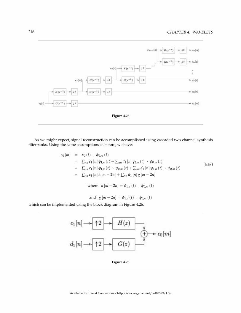
216 CHAPTER 4. WAVELETS
Figure 4.25
As we might expect, signal reconstruction can be accomplished using cascaded two-channel synthesisfilterbanks. Using the same assumptions as before, we have:
c0 [m] = x0 (t) · φ0,m (t)
= ∑nn c1 [n] φ1,n (t) + ∑nn d1 [n] ψ1,n (t) · φ0,m (t)
= ∑nn c1 [n] φ1,n (t) · φ0,m (t) + ∑nn d1 [n] ψ1,n (t) · φ0,m (t)
= ∑nn c1 [n] h [m− 2n] + ∑nn d1 [n] g [m− 2n]
(4.47)
where h [m− 2n] = φ1,n (t) · φ0,m (t)
and g [m− 2n] = ψ1,n (t) · φ0,m (t)
which can be implemented using the block diagram in Figure 4.26.
Figure 4.26
Available for free at Connexions <http://cnx.org/content/col10599/1.5>

217
The same procedure can be used to derive
c1 [m] = ∑nn
c2 [n] h [m− 2n] + ∑nn
d2 [n] g [m− 2n] (4.48)
from which we get the diagram in Figure 4.27.
Figure 4.27
To reconstruct from the kth level, we can use the iterated synthesis filterbank (Figure 4.28).
Figure 4.28
The table (Table 4.3) makes a direct comparison between wavelets and the two-channel orthogonal PR-FIR filterbanks.
Available for free at Connexions <http://cnx.org/content/col10599/1.5>

218 CHAPTER 4. WAVELETS
Discrete Wavelet Transform 2-Channel Orthogonal PR-FIRFilterbank
Analysis-LPF H(z−1) H0 (z)
Power Symmetry H (z) H(z−1) +
H (−z) H(−z−1) = 2
H0 (z) H0(z−1) +
H0 (−z) H0(−z−1) = 1
Analysis HPF G(z−1) H1 (z)
Spectral Reverse G (z) =±(z−PH
(−z−1)) , P is odd
H1 (z) =±(
z−(N−1)H0(−z−1)) , N is even
Synthesis LPF H (z) G0 (z) = 2z−(N−1)H0(z−1)
Synthesis HPF G (z) G1 (z) = 2z−(N−1)H1(z−1)
Table 4.3
From the table, we see that the discrete wavelet transform that we have been developing is identical totwo-channel orthogonal PR-FIR filterbanks in all but a couple details.
1. Orthogonal PR-FIR filterbanks employ synthesis filters with twice the gain of the analysis filters,whereas in the DWT the gains are equal.
2. Orthogonal PR-FIR filterbanks employ causal filters of length N, whereas the DWT filters are notconstrained to be causal.
For convenience, however, the wavelet filters H (z) and G (z) are usually chosen to be causal. For both tohave even impulse response length N, we require that P = N − 1.
4.3.11 Initialization of the Wavelet Transform33
The filterbanks developed in the module on the filterbanks interpretation of the DWT (Section 4.3.10) startwith the signal representation c0 [n] | n ∈ Z and break the representation down into wavelet coefficientsand scaling coefficients at lower resolutions (i.e., higher levels k). The question remains: how do we get theinitial coefficients c0 [n]?
From their definition, we see that the scaling coefficients can be written using a convolution:
c0 [n] = φ (t− n) · x (t)
=∫ ∞−∞ φ (t− n) x (t) dt
= φ (−t) ∗ x (t) |t=n′
(4.49)
which suggests that the proper initialization of wavelet transform is accomplished by passing thecontinuous-time input x (t) through an analog filter with impulse response φ (−t) and sampling its out-put at integer times (Figure 4.29).
33This content is available online at <http://cnx.org/content/m11018/2.2/>.
Available for free at Connexions <http://cnx.org/content/col10599/1.5>

219
Figure 4.29
Practically speaking, however, it is very difficult to build an analog filter with impulse response φ (−t)for typical choices of scaling function.
The most often-used approximation is to set c0 [n] = x [n]. The sampling theorem implies that thiswould be exact if φ (t) = sin(πt)
πt , though clearly this is not correct for general φ (t). Still, this technique issomewhat justified if we adopt the view that the principle advantage of the wavelet transform comes fromthe multi-resolution capabilities implied by an iterated perfect-reconstruction filterbank (with good filters).
4.3.12 Regularity Conditions, Compact Support, and Daubechies’ Wavelets34
Here we give a quick description of what is probably the most popular family of filter coefficients h [n] andg [n] — those proposed by Daubechies.
Recall the iterated synthesis filterbank. Applying the Noble identities, we can move the up-samplersbefore the filters, as illustrated in Figure 4.30.
34This content is available online at <http://cnx.org/content/m10495/2.8/>.
Available for free at Connexions <http://cnx.org/content/col10599/1.5>

220 CHAPTER 4. WAVELETS
Figure 4.30
The properties of the i-stage cascaded lowpass filter
H(i) (z) =i−1
∏k=0
H(
z2k)
, i ≥ 1 (4.50)
in the limit i → ∞ give an important characterization of the wavelet system. But how do we know thatlimit
i→∞H(i) (ejω) converges to a response in L2 ? In fact, there are some rather strict conditions on H
(ejω)
that must be satisfied for this convergence to occur. Without such convergence, we might have a finite-stageperfect reconstruction filterbank, but we will not have a countable wavelet basis for L2 . Below we presentsome "regularity conditions" on H
(ejω) that ensure convergence of the iterated synthesis lowpass filter.
NOTE: The convergence of the lowpass filter implies convergence of all other filters in the bank.
Let us denote the impulse response of H(i) (z) by h(i) [n]. Writing
H(i) (z) = H(
z2i−1)
H(i−1) (z)
in the time domain, we haveh(i) [n] = ∑
kkh [k] h(i−1)
[n− 2i−1k
]Now define the function
φ(i) (t) = 2i2 ∑
nnh(i) [n] I[n/2i ,n+1/2i) (t)
where I[a,b) (t) denotes the indicator function over the interval [a, b):
I[a,b) (t) =
1 if t ∈ [a, b)
0 if t /∈ [a, b)
Available for free at Connexions <http://cnx.org/content/col10599/1.5>

221
The definition of φ(i) (t) implies
h(i) [n] = 2−i2 φ(i) (t) , t ∈
[n2i ,
n + 12i
)(4.51)
h(i−1)[n− 2i−1k
]= 2−
i−12 φ(i−1) (2t− k) , t ∈
[n2i ,
n + 12i
)(4.52)
and plugging the two previous expressions into the equation for h(i) [n] yields
φ(i) (t) =√
2 ∑kk
h [k] φ(i−1) [2t− k] . (4.53)
Thus, if φ(i) (t) converges pointwise to a continuous function, then it must satisfy the scaling equation, sothat limit
i→∞φ(i) (t) = φ (t). Daubechies[9] showed that, for pointwise convergence of φ(i) (t) to a continuous
function in L2 , it is sufficient that H(ejω) can be factored as
H(
ejω)
=√
2(
1 + ejω
2
)P
R(
ejω)
, P ≥ 1 (4.54)
for R(ejω) such that
supω
(|R(
ejω)|)
< 2P−1 (4.55)
Here P denotes the number of zeros that H(ejω) has at ω = π. Such conditions are called regularity
conditions because they ensure the regularity, or smoothness of φ (t). In fact, if we make the previouscondition stronger:
supω
(|R(
ejω)|)
< 2P−1−` , ` ≥ 1 (4.56)
then limiti→∞
φ(i) (t) = φ (t) for φ (t) that is `-times continuously differentiable.
There is an interesting and important by-product of the preceding analysis. If h [n] is a causal length-Nfilter, it can be shown that h(i) [n] is causal with length Ni = 2i (N − 1) + 1. By construction, then, φ(i) [t]
will be zero outside the interval[0, 2i(N−1)+1
2i
). Assuming that the regularity conditions are satisfied so
that limiti→∞
φ(i) (t) = φ (t), it follows that φ (t) must be zero outside the interval [0, N − 1]. In this case
we say that φ (t) has compact support. Finally, the wavelet scaling equation implies that, when φ (t) iscompactly supported on [0, N − 1] and g [n] is length N, ψ (t) will also be compactly supported on theinterval [0, N − 1].
Daubechies constructed a family of H (z) with impulse response lengths N ∈ 4, 6, 8, 10, . . . whichsatisfy the regularity conditions. Moreover, her filters have the maximum possible number of zeros atω = π, and thus are maximally regular (i.e., they yield the smoothest possible φ (t) for a given supportinterval). It turns out that these filters are the maximally flat filters derived by Herrmann[14] long beforefilterbanks and wavelets were in vogue. In Figure 4.31 and Figure 4.32 we show φ (t), Φ (Ω), ψ (t), andΨ (Ω) for various members of the Daubechies’ wavelet system.
See Vetterli and Kovacivic[25] for a more complete discussion of these matters.
Available for free at Connexions <http://cnx.org/content/col10599/1.5>
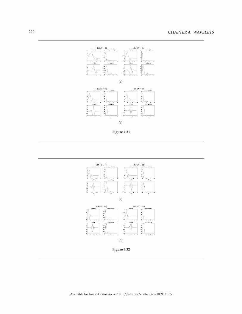
222 CHAPTER 4. WAVELETS
(a)
(b)
Figure 4.31
(a)
(b)
Figure 4.32
Available for free at Connexions <http://cnx.org/content/col10599/1.5>

223
4.3.13 Computing the Scaling Function: The Cascade Algorithm35
Given coefficients h [n] that satisfy the regularity conditions, we can iteratively calculate samples of φ (t)on a fine grid of points t using the cascade algorithm. Once we have obtained φ (t), the wavelet scalingequation can be used to construct ψ (t).
In this discussion we assume that H (z) is causal with impulse response length N. Recall, from ourdiscussion of the regularity conditions (p. 220), that this implies φ (t) will have compact support on theinterval [0, N − 1]. The cascade algorithm is described below.
1. Consider the scaling function at integer times t = m ∈ 0, . . . , N − 1:
φ (m) =√
2N−1
∑n=0
h (n) φ (2m− n)
Knowing that φ (t) = 0 for t /∈ [0, N − 1], the previous equation can be written using an NxN matrix.In the case where N = 4, we have
φ (0)
φ (1)
φ (2)
φ (3)
=√
2
h [0] 0 0 0
h [2] h [1] h [0] 0
0 h [3] h [2] h [1]
0 0 0 h [3]
φ (0)
φ (1)
φ (2)
φ (3)
(4.57)
where H =
h [0] 0 0 0
h [2] h [1] h [0] 0
0 h [3] h [2] h [1]
0 0 0 h [3]
The matrix H is structured as a row-decimated convolution matrix. From the matrix equation above((4.57)), we see that (φ (0) , φ (1) , φ (2) , φ (3))T must be (some scaled version of) the eigenvector of
H corresponding to eigenvalue(√
2)−1
. In general, the nonzero values of φ (n) | n ∈ Z, i.e.,
(φ (0) , φ (1) , . . . , φ (N − 1))T , can be calculated by appropriately scaling the eigenvector of the NxN
row-decimated convolution matrix H corresponding to the eigenvalue(√
2)−1
. It can be shown that
this eigenvector must be scaled so that ∑N−1n=0 φ (n) = 1.
2. Given φ (n) | n ∈ Z, we can use the scaling equation to determine
φ( n
2)| n ∈ Z
:
φ(m
2
)=√
2N−1
∑n=0
h [n] φ (m− n) (4.58)
This produces the 2N − 1 non-zero samples φ (0) , φ (1/2) , φ (1) , φ (3/2) , . . . , φ (N − 1).3. Given
φ( n
2)| n ∈ Z
, the scaling equation can be used to find
φ( n
4)| n ∈ Z
:
φ(m
4)
=√
2 ∑N−1n=0 h [n] φ
(m2 − n
)=√
2 ∑pp even h[ p
2]
φ(
m−p2
)=√
2 ∑pp h↑2 [p] φ 12[m− p]
(4.59)
where h↑2 [p] denotes the impulse response of H(z2), i.e., a 2-upsampled version of h [n], and where
φ 12[m] = φ
(m2). Note that
φ( n
4)| n ∈ Z
is the result of convolving h↑2 [n] with
φ 1
2[n]
.
35This content is available online at <http://cnx.org/content/m10486/2.6/>.
Available for free at Connexions <http://cnx.org/content/col10599/1.5>

224 CHAPTER 4. WAVELETS
4. Given
φ( n
4)| n ∈ Z
, another convolution yields
φ( n
8)| n ∈ Z
:
φ(m
8)
=√
2 ∑N−1n=0 h [n] φ
(m4 − n
)=√
2 ∑pp h↑4 [p] φ 14[m− p]
(4.60)
where h↑4 [n] is a 4-upsampled version of h [n] and where φ 14[m] = φ
(m4).
5. At the `th stage,
φ(
n2`
)is calculated by convolving the result of the `− 1th stage with a 2`−1-
upsampled version of h [n]:
φ 12`
(m) =√
2 ∑pp
h↑2`−1 [p] φ 12`−1
[m− p] (4.61)
For ` ' 10, this gives a very good approximation of φ (t). At this point, you could verify the key propertiesof φ (t), such as orthonormality and the satisfaction of the scaling equation.
In Figure 4.33 we show steps 1 through 5 of the cascade algorithm, as well as step 10, using Daubechies’db2 coefficients (for which N = 4).
Available for free at Connexions <http://cnx.org/content/col10599/1.5>

225
Figure 4.33
4.3.14 Finite-Length Sequences and the DWT Matrix36
The wavelet transform, viewed from a filterbank perspective, consists of iterated 2-channel analysis stageslike the one in Figure 4.34.
36This content is available online at <http://cnx.org/content/m10459/2.6/>.
Available for free at Connexions <http://cnx.org/content/col10599/1.5>

226 CHAPTER 4. WAVELETS
Figure 4.34
First consider a very long (i.e., practically infinite-length) sequence ck [m] | m ∈ Z. For every pair ofinput samples ck [2n] , ck [2n− 1] that enter the kth filterbank stage, exactly one pair of output samplesck+1 [n] , dk+1 [n] are generated. In other words, the number of output equals the number of input duringa fixed time interval. This property is convenient from a real-time processing perspective.
For a short sequence ck [m] | m ∈ 0, . . . , M− 1, however, linear convolution requires that we makean assumption about the tails of our finite-length sequence. One assumption could be
ck [m] = 0 , m ∈ 0, . . . , M− 1 (4.62)
In this case, the linear convolution implies that M nonzero inputs yield M+N2 − 1 outputs from each branch,
for a total of 2(
M+N2 − 1
)= M + N − 2 > M outputs. Here we have assumed that both H
(z−1) and
G(z−1) have impulse response lengths of N > 2, and that M and N are both even. The fact that each
filterbank stage produces more outputs than inputs is very disadvantageous in many applications.A more convenient assumption regarding the tails of ck [m] | m ∈ 0, . . . , M− 1 is that the data out-
side of the time window 0, . . . , M− 1 is a cyclic extension of data inside the time window. In other words,given a length-M sequence, the points outside the sequence are related to points inside the sequences via
ck [m] = ck [m + M] (4.63)
Recall that a linear convolution with an M-cyclic input is equivalent to a circular convolution with oneM-sample period of the input sequences. Furthermore, the output of this circular convolution is itself M-cyclic, implying our 2-downsampled branch outputs are cyclic with period M
2 . Thus, given an M-lengthinput sequence, the total filterbank output consists of exactly M values.
It is instructive to write the circular-convolution analysis fiterbank operation in matrix form. In (4.64)we give an example for filter length N = 4, sequence length N = 8, and causal synthesis filters H (z) andG (z).
ck+1 [0]
ck+1 [1]
ck+1 [2]
ck+1 [3]
dk+1 [0]
dk+1 [1]
dk+1 [2]
dk+1 [3]
=
h [0] h [1] h [2] h [3] 0 0 0 0
0 0 h [0] h [1] h [2] h [3] 0 0
0 0 0 0 h [0] h [1] h [2] h [3]
h [2] h [3] 0 0 0 0 h [0] h [1]
g [0] g [1] g [2] g [3] 0 0 0 0
0 0 g [0] g [1] g [2] g [3] 0 0
0 0 0 0 g [0] g [1] g [2] g [3]
g [2] g [3] 0 0 0 0 g [0] g [1]
ck [0]
ck [1]
ck [2]
ck [3]
ck [4]
ck [5]
ck [6]
ck [7]
(4.64)
Available for free at Connexions <http://cnx.org/content/col10599/1.5>

227
where
ck+1
dk+1
=
ck+1 [0]
ck+1 [1]
ck+1 [2]
ck+1 [3]
dk+1 [0]
dk+1 [1]
dk+1 [2]
dk+1 [3]
HM
GM
=
h [0] h [1] h [2] h [3] 0 0 0 0
0 0 h [0] h [1] h [2] h [3] 0 0
0 0 0 0 h [0] h [1] h [2] h [3]
h [2] h [3] 0 0 0 0 h [0] h [1]
g [0] g [1] g [2] g [3] 0 0 0 0
0 0 g [0] g [1] g [2] g [3] 0 0
0 0 0 0 g [0] g [1] g [2] g [3]
g [2] g [3] 0 0 0 0 g [0] g [1]
ck =
ck [0]
ck [1]
ck [2]
ck [3]
ck [4]
ck [5]
ck [6]
ck [7]
The matrices HM and GM have interesting properties. For example, the conditions
δ [m] = ∑nn
h [n] h [n− 2m]
g [n] = −1nh [N − 1− n]
imply that HM
GM
T HM
GM
=
HM
GM
HM
GM
T
= IM
where IM denotes the MxM identity matrix. Thus, it makes sense to define the MxM DWT matrix as
TM =
HM
GM
(4.65)
Available for free at Connexions <http://cnx.org/content/col10599/1.5>

228 CHAPTER 4. WAVELETS
whose transpose constitutes the MxM inverse DWT matrix:
TM−1 = TM
T (4.66)
Since the synthesis filterbank (Figure 4.35)
Figure 4.35
gives perfect reconstruction, and since the cascade of matrix operations TMTTM also corresponds to per-
fect reconstruction, we expect that the matrix operation TMT describes the action of the synthesis filterbank.
This is readily confirmed by writing the upsampled circular convolutions in matrix form:
ck [0]
ck [1]
ck [2]
ck [3]
ck [4]
ck [5]
ck [6]
ck [7]
=
h [0] 0 0 h [2] g [0] 0 0 g [2]
h [1] 0 0 h [3] g [1] 0 0 g [3]
h [2] h [0] 0 0 g [2] g [0] 0 0
h [3] h [1] 0 0 g [3] g [1] 0 0
0 h [2] h [0] 0 0 g [2] g [0] 0
0 h [3] h [1] 0 0 g [3] g [1] 0
0 0 h [2] h [0] 0 0 g [2] g [0]
0 0 h [3] h [1] 0 0 g [3] g [1]
ck+1 [0]
ck+1 [1]
ck+1 [2]
ck+1 [3]
dk+1 [0]
dk+1 [1]
dk+1 [2]
dk+1 [3]
(4.67)
where
HMT
GMT
= TMT =
h [0] 0 0 h [2] g [0] 0 0 g [2]
h [1] 0 0 h [3] g [1] 0 0 g [3]
h [2] h [0] 0 0 g [2] g [0] 0 0
h [3] h [1] 0 0 g [3] g [1] 0 0
0 h [2] h [0] 0 0 g [2] g [0] 0
0 h [3] h [1] 0 0 g [3] g [1] 0
0 0 h [2] h [0] 0 0 g [2] g [0]
0 0 h [3] h [1] 0 0 g [3] g [1]
So far we have concentrated on one stage in the wavelet decomposition; a two-stage decomposition isillustrated in Figure 4.36.
Available for free at Connexions <http://cnx.org/content/col10599/1.5>

229
Figure 4.36
The two-stage analysis operation (assuming circular convolution) can be expressed in matrix form asck+2
dk+2
dk+1
=
TM2
0
0 I M2
ck+1
dk+1
=
TM2
0
0 I M2
( TM
) (ck
) (4.68)
Similarly, a three-stage analysis could be implemented viack+3
dk+3
dk+2
dk+1
=
TM
40 0
0 I M4
0
0 0 I M2
TM
20
0 I M2
( TM
) (ck
)(4.69)
It should now be evident how to extend this procedure to 3 stages. As noted earlier, the correspondingsynthesis operations are accomplished by transposing the matrix products used in the analysis.
4.3.15 DWT Implementation using FFTs37
Finally, we say a few words about DWT implementation. Here we focus on a single DWT stage and assumecircular convolution, yielding an MxM DWT matrix TM . In the general case, MxM matrix multiplica-tion requires M2 multiplications. The DWT matrices, however, have a circular-convolution structure whichallows us to implement them using significantly less multiplies. Below we present some simple and rea-sonably efficient approaches for the implementation of TM and TM
T .We treat the inverse DWT first. Recall that in the lowpass synthesis branch, we upsample the input
before circularly convolving with H (z). Denoting the upsampled coefficient sequence by a [n], fast circularconvolution a [n] ∗ h [n] can be described as follows (using Matlab notation)
37This content is available online at <http://cnx.org/content/m10999/2.1/>.
Available for free at Connexions <http://cnx.org/content/col10599/1.5>

230 CHAPTER 4. WAVELETS
ifft( fft(a).*fft(h,length(a)) )
where we have assumed that length(a) ≥ length(h). 38 The highpass branch is handled similarly usingG (z), after which the two branch outputs are summed.
Next we treat the forward DWT. Recall that in the lowpass analysis branch, we circularly convolve theinput with H
(z−1) and then downsample the result. The fast circular convolution a [n] ∗ h [−n] can be
implemented using
wshift('1', ifft(fft(a).*fft(flipud(h),length(a))), length(h)-1 )
where wshift accomplishes a circular shift of the ifft output that makes up for the unwanted delay oflength(h)-1 samples imposed by the flipud operation. The highpass branch is handled similarly butwith filter G
(z−1). Finally, each branch is downsampled by factor two.
We note that the proposed approach is not totally efficient because downsampling is performed aftercircular convolution (and upsampling before circular convolution). Still, we have outlined this approachbecause it is easy to understand and still results in major saving when M is large: it converts the O
(M2)
matrix multiply into an O (Mlog2M) operation.
4.3.16 DWT Applications - Choice of phi(t)39
Transforms are signal processing tools that are used to give a clear view of essential signal characteristics.Fourier transforms are ideal for infinite-duration signals that contain a relatively small number of sinusoids:one can completely describe the signal using only a few coefficients. Fourier transforms, however, arenot well-suited to signals of a non-sinusoidal nature (as discussed earlier in the context of time-frequencyanalysis (Section 4.1.2)). The multi-resolution DWT is a more general transform that is well-suited to alarger class of signals. For the DWT to give an efficient description of the signal, however, we must choose awavelet ψ (t) from which the signal can be constructed (to a good approximation) using only a few stretchedand shifted copies.
We illustrate this concept in Figure 4.37 using two examples. On the left, we analyze a step-likewaveform, while on the right we analyze a chirp-like waveform. In both cases, we try DWTs basedon the Haar and Daubechies db10 wavelets and plot the log magnitudes of the transform coefficients[
ckT , dk
T , dk−1T , dk−2
T , . . . , d1T].
38When implementing the multi-level transform, you must ensure that the data length does not become shorter than the filter length!39This content is available online at <http://cnx.org/content/m11004/2.1/>.
Available for free at Connexions <http://cnx.org/content/col10599/1.5>

231
Figure 4.37
Observe that the Haar DWT yields an extremely efficient representation of the step-waveform: onlya few of the transform coefficients are nonzero. The db10 DWT does not give an efficient representation:many coefficients are sizable. This makes sense because the Haar scaling function is well matched to thestep-like nature of the time-domain signal. In contrast, the Haar DWT does not give an efficient represen-tation of the chirp-like waveform, while the db10 DWT does better. This makes sense because the sharpedges of the Haar scaling function do not match the smooth chirp signal, while the smoothness of the db10
wavelet yields a better match.
4.3.17 DWT Application - De-noising40
Say that the DWT for a particular choice of wavelet yields an efficient representation of a particular signalclass. In other words, signals in the class are well-described using a few large transform coefficients.
Now consider unstructured noise, which cannot be eifficiently represented by any transform, includingthe DWT. Due to the orthogonality of the DWT, such noise sequences make, on average, equal contributionsto all transform coefficients. Any given noise sequence is expected to yield many small-valued transformcoefficients.
Together, these two ideas suggest a means of de-noising a signal. Say that we perform a DWT on asignal from our well-matched signal class that has been corrupted by additive noise. We expect that largetransform coefficients are composed mostly of signal content, while small transform coefficients should be
40This content is available online at <http://cnx.org/content/m11000/2.1/>.
Available for free at Connexions <http://cnx.org/content/col10599/1.5>

232 CHAPTER 4. WAVELETS
composed mostly of noise content. Hence, throwing away the transform coefficients whose magnitudeis less than some small threshold should improve the signal-to-noise ratio. The de-noising procedure isillustrated in Figure 4.38.
Figure 4.38
Now we give an example of denoising a step-like waveform using the Haar DWT. In Figure 4.39, thetop right subplot shows the noisy signal and the top left shows it DWT coefficients. Note the presence ofa few large DWT coefficients, expected to contain mostly signal components, as well as the presence ofmany small-valued coefficients, expected to contain noise. (The bottom left subplot shows the DWT forthe original signal before any noise was added, which confirms that all signal energy is contained withina few large coefficients.) If we throw away all DWT coefficients whose magnitude is less than 0.1, we areleft with only the large coefficients (shown in the middle left plot) which correspond to the de-noised time-domain signal shown in the middle right plot. The difference between the de-noised signal and the originalnoiseless signal is shown in the bottom right. Non-zero error results from noise contributions to the largecoefficients; there is no way of distinguishing these noise components from signal components.
Available for free at Connexions <http://cnx.org/content/col10599/1.5>

233
Figure 4.39
Available for free at Connexions <http://cnx.org/content/col10599/1.5>

234 CHAPTER 4. WAVELETS
Available for free at Connexions <http://cnx.org/content/col10599/1.5>

Chapter 5
Multirate Signal Processing
5.1 Overview of Multirate Signal Processing1
Digital transformation of the sampling rate of signals, or signal processing with different sampling rates inthe system.
5.1.1 Applications
1. CD to DAT format change, for example.2. oversampling converters; which reduce performance requirements on anti-aliasing or reconstruction
filters3. bandwidth of individual channels is much less than the overall bandwidth4. Eyes and ears are not as sensitive to errors in higher frequency bands, so many coding schemes split
signals into different frequency bands and quantize higher-frequency bands with much less precision.
5.1.2 Outline of Multirate DSP material
1. General Rate-changing System (Section 5.1.3: General Rate-Changing Procedure)2. Integer-factor Interpolation and Decimation and Rational-factor Rate Changing (Section 5.2)3. Efficient Multirate Filter Structures (Section 5.3)4. Optimal Filter Design for Multirate Systems (Section 5.4)5. Multi-stage Multirate Systems (Section 5.5)6. Oversampling D/As (Section 5.6)7. Perfect-Reconstruction Filter Banks and Quadrature Mirror Filters (Section 5.7)
5.1.3 General Rate-Changing Procedure
This procedure is motivated by an analog-based method: one conceptually simple method to change thesampling rate is to simply convert a digital signal to an analog signal and resample it! (Figure 5.1)
1This content is available online at <http://cnx.org/content/m12777/1.3/>.
Available for free at Connexions <http://cnx.org/content/col10599/1.5>
235
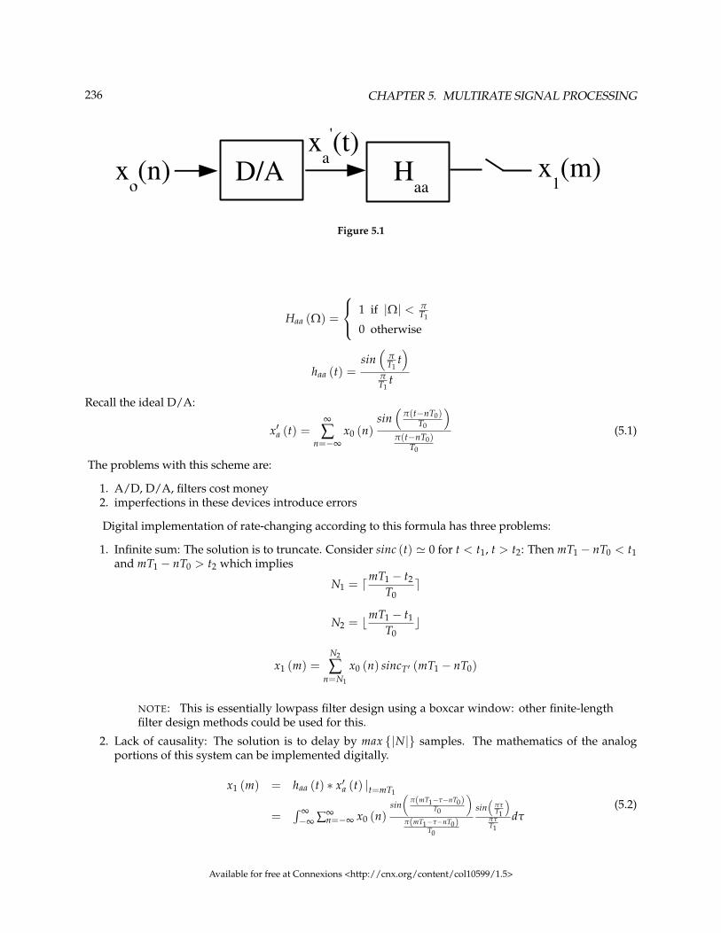
236 CHAPTER 5. MULTIRATE SIGNAL PROCESSING
Figure 5.1
Haa (Ω) =
1 if |Ω| < πT1
0 otherwise
haa (t) =sin(
πT1
t)
πT1
t
Recall the ideal D/A:
x′a (t) =∞
∑n=−∞
x0 (n)sin(
π(t−nT0)T0
)π(t−nT0)
T0
(5.1)
The problems with this scheme are:
1. A/D, D/A, filters cost money2. imperfections in these devices introduce errors
Digital implementation of rate-changing according to this formula has three problems:
1. Infinite sum: The solution is to truncate. Consider sinc (t) ' 0 for t < t1, t > t2: Then mT1 − nT0 < t1and mT1 − nT0 > t2 which implies
N1 = dmT1 − t2
T0e
N2 = bmT1 − t1
T0c
x1 (m) =N2
∑n=N1
x0 (n) sincT′ (mT1 − nT0)
NOTE: This is essentially lowpass filter design using a boxcar window: other finite-lengthfilter design methods could be used for this.
2. Lack of causality: The solution is to delay by max |N| samples. The mathematics of the analogportions of this system can be implemented digitally.
x1 (m) = haa (t) ∗ x′a (t) |t=mT1
=∫ ∞−∞ ∑∞
n=−∞ x0 (n)sin(
π(mT1−τ−nT0)T0
)π(mT1−τ−nT0)
T0
sin(
πτT1
)πτT1
dτ(5.2)
Available for free at Connexions <http://cnx.org/content/col10599/1.5>

237
x1 (m) = ∑∞n=−∞ x0 (n)
sin( πT′ (mT1−nT0))
πT′ (mT1−nT0)
|T ′=maxT0,T1
= ∑∞n=−∞ x0 (n) sincT′ (mT1 − nT0)
(5.3)
So we have an all-digital formula for exact digital-to-digital rate changing!3. Cost of computing sincT′ (mT1 − nT0): The solution is to precompute the table of sinc (t) values. How-
ever, if T1T0
is not a rational fraction, an infinite number of samples will be needed, so some approxi-mation will have to be tolerated.
NOTE: Rate transformation of any rate to any other rate can be accomplished digitally witharbitrary precision (if some delay is acceptable). This method is used in practice in manycases. We will examine a number of special cases and computational improvements, but insome sense everything that follows are details; the above idea is the central idea in multiratesignal processing.
Useful references for the traditional material (everything except PRFBs) are Crochiere and Rabiner, 1981[7] and Crochiere and Rabiner, 1983 [8]. A more recent tutorial is Vaidyanathan [24]; see also Rioul andVetterli [20]. References to most of the original papers can be found in these tutorials.
5.2 Interpolation, Decimation, and Rate Changing by Integer Fractions2
5.2.1 Interpolation: by an integer factor L
Interpolation means increasing the sampling rate, or filling in in-between samples. Equivalent to samplinga bandlimited analog signal L times faster. For the ideal interpolator,
X1 (ω) =
X0 (Lω) if |ω| < πL
0 if πL ≤ |ω| ≤ π
(5.4)
We wish to accomplish this digitally. Consider (5.5) and Figure 5.2.
y (m) =
X0(m
L)
if m = 0,± (L) ,± (2L) , . . . 0 otherwise
(5.5)
2This content is available online at <http://cnx.org/content/m12801/1.3/>.
Available for free at Connexions <http://cnx.org/content/col10599/1.5>

238 CHAPTER 5. MULTIRATE SIGNAL PROCESSING
Figure 5.2
The DTFT of y (m) is
Y (ω) = ∑∞m=−ω y (m) e−(jωm)
= ∑∞n=−∞ x0 (n) e−(jωLn)
= ∑∞n=−∞ x (n) e−(jωLn)
= X0 (ωL)
(5.6)
Since X0 (ω′) is periodic with a period of 2π, X0 (Lω) = Y (ω) is periodic with a period of 2πL (see Fig-
ure 5.3).
Figure 5.3
By inserting zero samples between the samples of x0 (n), we obtain a signal with a scaled frequencyresponse that simply replicates X0 (ω′) L times over a 2π interval!
Obviously, the desired x1 (m) can be obtained simply by lowpass filtering y (m) to remove the replicas.
x1 (m) = y (m) ∗ hL (m) (5.7)
Given
HL (m) =
1 if |ω| < πL
0 if πL ≤ |ω| ≤ π
In practice, a finite-length lowpass filter is designed using any of the methods studied so far (Figure 5.4(Interpolator Block Diagram)).
Available for free at Connexions <http://cnx.org/content/col10599/1.5>

239
Interpolator Block Diagram
Figure 5.4
5.2.2 Decimation: sampling rate reduction (by an integer factor M)
Let y (m) = x0 (Lm) (Figure 5.5)
Figure 5.5
That is, keep only every Lth sample (Figure 5.6)
Figure 5.6
Available for free at Connexions <http://cnx.org/content/col10599/1.5>

240 CHAPTER 5. MULTIRATE SIGNAL PROCESSING
In frequency (DTFT):
Y (ω) = ∑∞m=−∞ y (m) e−(jωm)
= ∑∞m=−∞ x0 (Mm) e−(jωm)
= ∑∞n=−∞ x0 (n) ∑∞
k=−∞ δ (n−Mk) e−(jω nM )|n=Mm
= ∑∞n=−∞ x0 (n) ∑∞
k=−∞ δ (n−Mk) e−(jω′n)|ω ′= ω
M
= DTFT [x0 (n)] ∗ DTFT [∑ δ (n−Mk)]
(5.8)
Now DTFT [∑ δ (n−Mk)] = 2π ∑M−1k=0 X (k) δ
(ω′ − 2πk
M
)for |ω| < π as shown in homework #1 , where
X (k) is the DFT of one period of the periodic sequence. In this case, X (k) = 1 for k ∈ 0, 1, . . . , M− 1 andDTFT [∑ δ (n−Mk)] = 2π ∑M−1
k=0 δ(
ω′ − 2πkM
).
DTFT [x0 (n)] ∗ DTFT [∑ δ (n−Mk)] = X0 (ω′) ∗ 2π ∑M−1k=0 δ
(ω′ − 2πk
M
)= 1
2π
∫ π−π X0 (µ′)
(2π ∑M−1
k=0 δ(
ω′ − µ′ − 2πkM
))dµ ′
= ∑M−1k=0 X0
(ω′ − 2πk
M
) (5.9)
so Y (ω) = ∑M−1k=0 X0
(ωM −
2πkM
)i.e., we get digital aliasing.(Figure 5.7)
Figure 5.7
Usually, we prefer not to have aliasing, so the downsampler is preceded by a lowpass filter to removeall frequency components above |ω| < π
M (Figure 5.8).
Available for free at Connexions <http://cnx.org/content/col10599/1.5>

241
Figure 5.8
5.2.3 Rate-Changing by a Rational Fraction L/M
This is easily accomplished by interpolating by a factor of L, then decimating by a factor of M (Figure 5.9).
Figure 5.9
The two lowpass filters can be combined into one LP filter with the lower cutoff,
H (ω) =
1 if |ω| < πmaxL,M
0 if πmaxL,M ≤ |ω| ≤ π
Obviously, the computational complexity and simplicity of implementation will depend on LM : 2/3 will be
easier to implement than 1061/1060!
5.3 Efficient Multirate Filter Structures3
Rate-changing appears expensive computationally, since for both decimation and interpolation the lowpassfilter is implemented at the higher rate. However, this is not necessary.
5.3.1 Interpolation
For the interpolator, most of the samples in the upsampled signal are zero, and thus require no computation.(Figure 5.10)
3This content is available online at <http://cnx.org/content/m12800/1.3/>.
Available for free at Connexions <http://cnx.org/content/col10599/1.5>

242 CHAPTER 5. MULTIRATE SIGNAL PROCESSING
Figure 5.10
For m = LbmL c+ mmodL and p = mmodL,
x1 (m) = ∑N2m=N1
hLp (m) y (m)
= ∑N2L
k= N1L
gp (k) x0(bm
L c − k) (5.10)
gp (n) = h (Ln + p)
Pictorially, this can be represented as in Figure 5.11.
Available for free at Connexions <http://cnx.org/content/col10599/1.5>

243
Figure 5.11
These are called polyphase structures, and the gp (n) are called polyphase filters.Computational costIf h (m) is a length-N filter:
• No simplification: NT1
= LNT0
computationssec
• Polyphase structure:(
L LN
1To
0
)computations
sec = NT0
where L is the number of filters, NL is the taps/filter,
and 1T0
is the rate.
Thus we save a factor of L by not being dumb.
NOTE: For a given precision, N is proportional to L, (why?), so the computational cost doesincrease with the interpolation rate.
QUESTION: Can similar computational savings be obtained with IIR structures?
5.3.2 Efficient Decimation Structures
We only want every Mth output, so we compute only the outputs of interest. (Figure 5.12 (PolyphaseDecimation Structure))
x1 (m) =N2
∑k=N1
x0 (Lm− k) h (k)
Available for free at Connexions <http://cnx.org/content/col10599/1.5>

244 CHAPTER 5. MULTIRATE SIGNAL PROCESSING
Polyphase Decimation Structure
Figure 5.12
The decimation structures are flow-graph reversals of the interpolation structure. Although direct im-plementation of the full filter for every Mth sample is obvious and straightforward, these polyphase struc-tures give some idea as to how one might evenly partition the computation over M cycles.
5.3.3 Efficient L/M rate changers
Interpolate by L and decimate by M (Figure 5.13).
Figure 5.13
Combine the lowpass filters (Figure 5.14).
Figure 5.14
We can couple the lowpass filter either to the interpolator or the decimator to implement it efficiently(Figure 5.15).
Available for free at Connexions <http://cnx.org/content/col10599/1.5>

245
Figure 5.15
Of course we only compute the polyphase filter output selected by the decimator.Computational CostEvery T1 = M
L T0seconds, compute one polyphase filter of length NL , or
NL
T1=
NL
ML T0
=N
MT0
multipliessecond
However, note that N is proportional to max L, M.
5.4 Filter Design for Multirate Systems4
The filter design techniques5 learned earlier can be applied to the design of filters in multirate systems, witha few twists.
Example 5.1Design a factor-of-L interpolator for use in a CD player, we might wish that the out-of-band errorbe below the least significant bit, or 96dB down, and < 0.05% error in the passband, so thesespecifications could be used for optimal L∞ filter design.
In a CD player, the sampling rate is 44.1kHz, corresponding to a Nyquist frequency of 22.05kHz, butthe sampled signal is bandlimited to 20kHz. This leaves a small transition band, from 20kHz to 24.1kHz.However, note that in any case where the signal spectrum is zero over some band, this introduces otherzero bands in the scaled, replicated spectrum (Figure 5.16).
4This content is available online at <http://cnx.org/content/m12773/1.3/>.5Digital Filter Design <http://cnx.org/content/col10285/latest/>
Available for free at Connexions <http://cnx.org/content/col10599/1.5>

246 CHAPTER 5. MULTIRATE SIGNAL PROCESSING
Figure 5.16
So we need only control the filter response in the stopbands over the frequency regions with nonzeroenergy. (Figure 5.17)
Figure 5.17
The extra "don’t care" bands allow a given set of specifications to be satisfied with a shorter-length filter.
5.4.1 Direct polyphase filter design
Note that in an integer-factor interpolator, each set of output samples x1 (Ln + p), p = 0, 1, . . . , L− 1,is created by a different polyphase filter gp (n), which has no interaction with the other polyphase filtersexcept in that they each interpolate the same signal. We can thus treat the design of each polyphase filterindependently, as an N
L -length filter design problem. (Figure 5.18)
Figure 5.18
Available for free at Connexions <http://cnx.org/content/col10599/1.5>

247
Each gp (n) produces samples x1 (Ln + p) = x0(n + p
L), where n + p
L is not an integer. That is, gp (n) isto produce an output signal (at a T0 rate) that is x0 (n) time-advanced by a non-integer advance p
L .The desired response of this polyphase filter is thus
HDp (ω) = ejωp
L
for |ω| ≤ π, an all-pass filter with a linear, non-integer, phase. Each polyphase filter can be designedindependently to approximate this response according to any of the design criteria developed so far.
Exercise 5.4.1 (Solution on p. 259.)What should the polyphase filter for p = 0 be?
Example 5.2: Least-squares Polyphase Filter Design
Deterministic x(n): Minimize∞
∑n=−∞
(|x (n)− xd (n) |)2
Given x (n) = x (n) ∗ h (n) and xd (n) = x (n) ∗ hd (n). Using Parseval’s theorem, this be-comes
min
∑∞n=−∞ (|x (n)− xd (n) |)2
= min
1
2π
∫ π−π (|X (ω) H (ω)− X (ω) Hd (ω) |)2dω
= min
1
2π
∫ π−π |H (ω)− Hd (ω) |(|X (ω) |)2dω
(5.11)
This is simply weighted least squares design, with (|X (ω) |)2 as the weighting function.stochastic X(ω):
min
E[(|x (n)− xd (n) |)2
]= E
[(|x (n) ∗ (h (n)− hd (n)) |)2
]= min
1
2π
∫ π−π (|Hd (ω)− H (ω) |)2Sxx (ω) dω
(5.12)
Sxx (ω) is the power spectral density of x.
Sxx (ω) = DTFT [rxx (k)]
rxx (k) = E[x (k + l) x (l)∗
]Again, a weighted least squares filter design problem.
ProblemIs it feasible to use IIR polyphase filters?
SolutionThe recursive feedback of previous outputs means that portions of each IIR polyphase filter mustbe computed for every input sample; this usually makes IIR filters more expensive than FIR im-plementations.
Available for free at Connexions <http://cnx.org/content/col10599/1.5>

248 CHAPTER 5. MULTIRATE SIGNAL PROCESSING
5.5 Multistage Multirate Systems6
Multistage multirate systems are often more efficient. Suppose one wishes to decimate a signal by an integerfactor M, where M is a composite integer M = M1M2 . . . Mp = ∏
pi=1 Mi. A decimator can be implemented
in a multistage fashion by first decimating by a factor M1 , then decimating this signal by a factor M2 , etc.(Figure 5.19 (Multistage decimator))
Multistage decimator
Figure 5.19
Multistage implementations are of significant practical interest only if they offer significant computa-tional savings. In fact, they often do!
The computational cost of a single-stage interpolator is:
NMT0
tapssec
The computational cost of a multistage interpolator is:
N1
M1T0+
N2
M1M2T0+ · · ·+
Np
MT0
The first term is the most significant, since the rate is highest. Since Ni ∝ Mi for a lowpass filter, it is notimmediately clear that a multistage system should require less computation. However, the multistage struc-ture relaxes the requirements on the filters, which reduces their length and makes the overall computationless.
5.5.1 Filter design for Multi-stage Structures
Ostensibly, the first-stage filter must be a lowpass filter with a cutoff at πM1
, to prevent aliasing after thedownsampler. However, note that aliasing outside the final overall passband |ω| < π
M is of no concern,since it will be removed by later stages. We only need prevent aliasing into the band |ω| < π
M ; thus
6This content is available online at <http://cnx.org/content/m12803/1.3/>.
Available for free at Connexions <http://cnx.org/content/col10599/1.5>

249
we need only specify the passband over the interval |ω| < πM , and the stopband over the intervals ω ∈[
2πkM1− π
M , 2πkM1
+ πM
], for k ∈ 1, . . . , M− 1. (Figure 5.20)
Figure 5.20
Of course, we don’t want gain in the transition bands, since this would need to be suppressed later,but otherwise we don’t care about the response in those regions. Since the transition bands are so large,the required filter turns out to be quite short. The final stage has no "don’t care" regions; however, it isoperating at a low rate, so it is relatively unimportant if the final filter turns out to be rather long!
5.5.2 L-infinity Tolerances on the Pass and Stopbands
The overall response is a cascade of multiple filters, so the worst-case overall passband deviation, assumingall the peaks just happen to line up, is
1 + δpov =p
∏i=1
1 + δpi
1− δpov =p
∏i=1
1− δpi
So one could choose all filters to have equal specifications and require for each-stage filter. For δpov 1,
1 + δ+pi≤ p√
1 + δpov ' 1 + p−1δpov
1− δ−pi≤ p√
1− δpov ' 1− p−1δpov
Alternatively, one can design later stages (at lower computation rates) to compensate for the passbandripple in earlier stages to achieve exceptionally accurate passband response.
δs remains essentially unchanged, since the worst-case scenario is for the error to alias into the passbandand undergo no further suppression in subsequent stages.
5.5.3 Interpolation
Interpolation is the flow-graph reversal of the multi-stage decimator. The first stage has a cutoff at πL (Fig-
ure 5.21):
Available for free at Connexions <http://cnx.org/content/col10599/1.5>

250 CHAPTER 5. MULTIRATE SIGNAL PROCESSING
Figure 5.21
However, all subsequent stages have large bands without signal energy, due to the earlier stages (Fig-ure 5.22):
Figure 5.22
The order of the filters is reversed, but otherwise the filters are identical to the decimator filters.
5.5.4 Efficient Narrowband Lowpass Filtering
A very narrow lowpass filter requires a very long FIR filter to achieve reasonable resolution in the frequencyresponse. However, were the input sampled at a lower rate, the cutoff frequency would be correspondinglyhigher, and the filter could be shorter!
The transition band is also broader, which helps as well. Thus, Figure 5.23 can be implemented asFigure 5.24.
Figure 5.23
Available for free at Connexions <http://cnx.org/content/col10599/1.5>

251
Figure 5.24
and in practice the inner lowpass filter can be coupled to the decimator or interpolator filters. If the deci-mator and interpolator are implemented as multistage structures, the overall algorithm can be dramaticallymore efficient than direct implementation!
5.6 DFT-Based Filterbanks7
One common application of multirate processing arises in multirate, multi-channel filter banks (Fig-ure 5.25).
Figure 5.25
One application is separating frequency-division-multiplexed channels. If the filters are narrowband,the output channels can be decimated without significant aliasing.
Such structures are especially attractive when they can be implemented efficiently. For example, if
the filters are simply frequency modulated (by e−(j 2πkL n)) versions of each other, they can be efficiently
implemented using FFTs!Furthermore, there are classes of filters called perfect reconstruction filters which are of finite length
but from which the signal can be reconstructed exactly (using all M channels), even though the output ofeach channel experiences aliasing in the decimation step. These types of filterbanks have received a lot ofresearch attention, culminating in wavelet theory and techniques.
7This content is available online at <http://cnx.org/content/m12771/1.3/>.
Available for free at Connexions <http://cnx.org/content/col10599/1.5>

252 CHAPTER 5. MULTIRATE SIGNAL PROCESSING
5.6.1 Uniform DFT Filter Banks
Suppose we wish to split a digital input signal into N frequency bands, uniformly spaced at center fre-
quencies ωk = 2πkN , for 0 ≤ k ≤ N − 1. Consider also a lowpass filter h (n), H (ω) '
1 if |ω| < πN
0 otherwise.
Bandpass filters can be constructed which have the frequency response
Hk (ω) = H(
ω +2πkN
)from
hk (n) = h (n) e−(j 2πknN )
The output of the kth bandpass filter is simply (assume h (n) are FIR)
x (n) ∗ hk (n) = ∑M−1m=0 x (n−m) h (m) e−(j 2πkm
N )
= yk (n)(5.13)
This looks suspiciously like a DFT, except that M 6= N, in general. However, if we fix M =N, then we can compute all yk (n) outputs simultaneously using an FFT of x (n−m) h (m): Thekth FFT frequency output = yk (n)! So the cost of computing all of these filter banks outputs is O [NlogN],rather than N2, per a given n. This is very useful for efficient implementation of transmultiplexors (FDMto TDM).
Exercise 5.6.1 (Solution on p. 259.)How would we implement this efficiently if we wanted to decimate the individual channels
yk (n) by a factor of N, to their approximate Nyquist bandwidth?Exercise 5.6.2 (Solution on p. 259.)
Do you expect significant aliasing? If so, how do you propose to combat it? Efficiently?Exercise 5.6.3 (Solution on p. 259.)
How might one convert from N input channels into an FDM signal efficiently? (Figure 5.26)
Figure 5.26
NOTE: Such systems are used throughout the telephone system, satellite communication links,etc.
Available for free at Connexions <http://cnx.org/content/col10599/1.5>

253
5.7 Quadrature Mirror Filterbanks (QMF)8
Although the DFT filterbanks are widely used, there is a problem with aliasing in the decimated channels.At first glance, one might think that this is an insurmountable problem and must simply be accepted.Clearly, with FIR filters and maximal decimation, aliasing will occur. However, a simple example willshow that it is possible to exactly cancel out aliasing under certain conditions!!!
Consider the following trivial filterbank system, with two channels. (Figure 5.27)
Figure 5.27
Note^x (n) = x (n) with no error whatsoever, although clearly aliasing occurs in both channels! Note
that the overall data rate is still the Nyquist rate, so there are clearly enough degrees of freedom availableto reconstruct the data, if the filterbank is designed carefully. However, this isn’t splitting the data intoseparate frequency bands, so one questions whether something other than this trivial example could work.
Let’s consider a general two-channel filterbank, and try to determine conditions under which aliasingcan be cancelled, and the signal can be reconstructed perfectly (Figure 5.28).
Figure 5.28
Let’s derive^x (n), using z-transforms, in terms of the components of this system. Recall (Figure 5.29) is
equivalent toY (z) = H (z) X (z)
Y (ω) = H (ω) X (ω)
8This content is available online at <http://cnx.org/content/m12770/1.3/>.
Available for free at Connexions <http://cnx.org/content/col10599/1.5>

254 CHAPTER 5. MULTIRATE SIGNAL PROCESSING
Figure 5.29
and note that (Figure 5.30) is equivalent to
Y (z) =∞
∑m=−∞
x (m) z−(Lm) = x(
zL)
Y (ω) = X (Lω)
Figure 5.30
and (Figure 5.31) is equivalent to
Y (z) =1M
M−1
∑k=0
X(
z1M Wk
M
)
Y (ω) =1M
M−1
∑k=0
X(
ω
M+
2πkM
)
Figure 5.31
Y (z) is derived in the downsampler as follows:
Y (z) =∞
∑m=−∞
x (Mm) z−m
Let n = Mm and m = nM , then
Y (z) =∞
∑n=−∞
x (n)∞
∑p=−∞
δ (n−Mp) z−nM
Available for free at Connexions <http://cnx.org/content/col10599/1.5>

255
Nowx (n) ∑∞
p=−∞ δ (n−Mp) = IDFT[
x (ω) ∗ 2πM ∑M−1
k=0 δ(
ω− 2πkM
)]= IDFT
[2πM ∑M−1
k=0 X(
ω− 2πkM
)]= 1
M ∑M−1k=0 X (n) W−nk
M |W M=e−
j2πM
(5.14)
soY (z) = ∑∞
n=−∞
(1M ∑M−1
k=0 x (n) W−nkM
)z−
nM
= 1M ∑M−1
k=0 x (n)(
W+kM z
1M
)−n
= 1M ∑M−1
k=0 X(
z1M Wk
M
) (5.15)
Armed with these results, let’s determine^X (z)⇔^
x (n). (Figure 5.32)
Figure 5.32
NoteU1 (z) = X (z) H0 (z)
U2 (z) =12
1
∑k=0
X(
z12 e−
j2πk2
)H0
(z
12 e−(jπk)
)=
12
X(
z12
)H0
(z
12
)+
12
X(−z
12
)H0
(−z
12
)U3 (z) =
12
X (z) H0 (z) +12
X (−z) H0 (−z)
U4 (z) =12
F0 (z) H0 (z) X (z) +12
F0 (z) H0 (−z) X (−z)
and
L4 (z) =12
F1 (z) H1 (z) X (z) +12
F1 (z) H1 (−z) X (−z) =12
F1 (z) H1 (z) X (z) +12
F1 (z) H1 (−z) X (−z)
Finally then,
^X (z) = U4 (z)+ L4 (z) = 1
2 (H0 (z) F0 (z) X (z) + H0 (−z) F0 (z) X (−z) + H1 (z) F1 (z) X (z) + H1 (−z) F1 (z) X (−z)) =12 (H0 (z) F0 (z) + H1 (z) F1 (z)) X (z)+ 1
2 (H0 (−z) F0 (z) + H1 (−z) F1 (z)) X (−z)(5.16)
Note that the X (−z)→ X (ω + π) corresponds to the aliasing terms!There are four things we would like to have:
Available for free at Connexions <http://cnx.org/content/col10599/1.5>

256 CHAPTER 5. MULTIRATE SIGNAL PROCESSING
1. No aliasing distortion2. No phase distortion (overall linear phase→ simple time delay)3. No amplitude distortion4. FIR filters
No aliasing distortion
By insisting that H0 (−z) F0 (z) + H1 (−z) F1 (z) = 0, the X (−z) component of^X (z) can be removed, and
all aliasing will be eliminated! There may be many choices for H0, H1, F0, F1 that eliminate aliasing, butmost research has focused on the choice
F0 (z) = H1 (−z) : F1 (z) = −H0 (−z)
We will consider only this choice in the following discussion.Phase distortion
The transfer function of the filter bank, with aliasing cancelled, becomes T (z) =12 (H0 (z) F0 (z) + H1 (z) F1 (z)), which with the above choice becomes T (z) =12 (H0 (z) H1 (−z)− H1 (z) H0 (−z)). We would like T (z) to correspond to a linear-phase filter toeliminate phase distortion: Call
P (z) = H0 (z) H1 (−z)
Note thatT (z) =
12
(P (z)− P (−z))
Note that P (−z) ⇔ (−1)n p (n), and that if p (n) is a linear-phase filter, (−1)n p (n) is also (perhaps of theopposite symmetry). Also note that the sum of two linear-phase filters of the same symmetry (i.e., length ofp (n) must be odd) is also linear phase, so if p (n) is an odd-length linear-phase filter, there will be no phasedistortion. Also note that
Z−1 (p (z)− p (−z)) = p (n)− (−1)n p (n) =
2p (n) if n is odd
0 if n is even
means p (n) = 0, when n is even. If we choose h0 (n) and h1 (n) to be linear phase, p (n) will also be linearphase. Thus by choosing h0 (n) and h1 (n) to be FIR linear phase, we eliminate phase distortion and get FIRfilters as well (condition 4).Amplitude distortionAssuming aliasing cancellation and elimination of phase distortion, we might also desire no amplitude
distortion ( |T (ω) | = 1). All of these conditions require
T (z) =12
(H0 (z) H1 (−z)− H1 (z) H0 (−z)) = cz−D
where c is some constant and D is a linear phase delay. c = 1 for |T (ω) | = 1. It can be shown by consideringthat the following can be satisfied!
T (z) = P (z)− P (−z) = 2cz−D ⇔
2p (z) = 2cδ (n− D) if n is odd
p (n) = anything if n is even
Thus we require
P (z) =N′
∑n=0
p (2n) z−(2n) + z−D
Available for free at Connexions <http://cnx.org/content/col10599/1.5>

257
Any factorization of a P (z) of this form, P (z) = A (z) B (z) can lead to a Perfect Reconstruction filter bankof the form
H0 (z) = A (z)
H1 (−z) = B (z)
[This result is attributed to Vetterli.] A well-known special case (Smith and Barnwell)
H1 (z) = −(
z−(2D)+1H0
(−z−1
))Design techniques exist for optimally choosing the coefficients of these filters, under all of these constraints.
Quadrature Mirror Filters
H1 (z) = H0 (−z)⇔ H1 (ω) = H0 (π + ω) = H∗0 (π −ω) (5.17)
for real-valued filters. The frequency response is "mirrored" around ω = π2 . This choice leads to T (z) =
H02 (z)− H0
2 (−z): it can be shown that this can be a perfect reconstruction system only if
H0 (z) = c0z−(2n0) + c1z−(2n1)
which isn’t a very flexible choice of filters, and not a very good lowpass! The Smith and Barnwell approachis more commonly used today.
5.8 M-Channel Filter Banks9
The theory of M-band QMFBs and PRFBs has been investigated recently. Some results are available.
5.8.1 Tree-structured filter banks
Once we have a two-band PRFB, we can continue to split the subbands with similar systems! (Figure 5.33)
Figure 5.33
Thus we can recursively decompose a signal into 2p bands, each sampled at 2pth the rate of the originalsignal, and reconstruct exactly! Due to the tree structure, this can be quite efficient, and in fact close to theefficiency of an FFT filter bank, which does not have perfect reconstruction.
9This content is available online at <http://cnx.org/content/m12775/1.3/>.
Available for free at Connexions <http://cnx.org/content/col10599/1.5>

258 CHAPTER 5. MULTIRATE SIGNAL PROCESSING
5.8.2 Wavelet decomposition
We need not split both the upper-frequency and lower-frequency bands identically. (Figure 5.34)
Figure 5.34
This is good for image coding, because the energy tends to be distributed such that after a waveletdecomposition, each band has roughly equal energy.
Available for free at Connexions <http://cnx.org/content/col10599/1.5>

259
Solutions to Exercises in Chapter 5
Solution to Exercise 5.4.1 (p. 247)A delta function: h0 (n) = δ (n′)
Solution to Exercise 5.6.1 (p. 252)Simply step by N time samples between FFTs.
Solution to Exercise 5.6.2 (p. 252)Aliasing should be expected. There are two ways to reduce it:
1. Decimate by less ("oversample" the individual channels) such as decimating by a factor of N2 . This is
efficiently done by time-stepping by the appropriate factor.2. Design better (and thus longer) filters, say of length LN. These can be efficiently computed by pro-
ducing only N (every Lth) FFT outputs using simplified FFTs.
Solution to Exercise 5.6.3 (p. 252)Use an FFT and an inverse FFT for the modulation (TDM to FDM) and demodulation (FDM to TDM),
respectively.
Available for free at Connexions <http://cnx.org/content/col10599/1.5>

260 CHAPTER 5. MULTIRATE SIGNAL PROCESSING
Available for free at Connexions <http://cnx.org/content/col10599/1.5>

Chapter 6
Digital Filter Structures andQuantization Error Analysis
6.1 Filter Structures
6.1.1 Filter Structures1
A realizable filter must require only a finite number of computations per output sample. For linear, causal,time-Invariant filters, this restricts one to rational transfer functions of the form
H (z) =b0 + b1z−1 + · · ·+ bmz−m
1 + a1z−1 + a2z−2 + · · ·+ anz−n
Assuming no pole-zero cancellations, H (z) is FIR if ai = 0 , i > 0 , and IIR otherwise. Filter structuresusually implement rational transfer functions as difference equations.
Whether FIR or IIR, a given transfer function can be implemented with many different filter structures.With infinite-precision data, coefficients, and arithmetic, all filter structures implementing the same transferfunction produce the same output. However, different filter strucures may produce very different errorswith quantized data and finite-precision or fixed-point arithmetic. The computational expense and memoryusage may also differ greatly. Knowledge of different filter structures allows DSP engineers to trade offthese factors to create the best implementation.
6.1.2 FIR Filter Structures2
Consider causal FIR filters: y (n) = ∑M−1k=0 h (k) x (n− k); this can be realized using the following structure
1This content is available online at <http://cnx.org/content/m11917/1.3/>.2This content is available online at <http://cnx.org/content/m11918/1.2/>.
Available for free at Connexions <http://cnx.org/content/col10599/1.5>
261

262 CHAPTER 6. DIGITAL FILTER STRUCTURES AND QUANTIZATION ERRORANALYSIS
Figure 6.1
or in a different notation
Figure 6.2
Available for free at Connexions <http://cnx.org/content/col10599/1.5>

263
(a)
(b)
(c)
Figure 6.3
This is called the direct-form FIR filter structure.There are no closed loops (no feedback) in this structure, so it is called a non-recursive structure. Since
any FIR filter can be implemented using the direct-form, non-recursive structure, it is always possible toimplement an FIR filter non-recursively. However, it is also possible to implement an FIR filter recursively,and for some special sets of FIR filter coefficients this is much more efficient.
Example 6.1
y (n) =M−1
∑k=0
x (n− k)
where
h (k) =
0, 0, 1ˆ
k=0
, 1, . . . , 1, 1ˆ
k=M−1
, 0, 0, 0, . . .
But note that
y (n) = y (n− 1) + x (n)− x (n−M)
This can be implemented as
Available for free at Connexions <http://cnx.org/content/col10599/1.5>

264 CHAPTER 6. DIGITAL FILTER STRUCTURES AND QUANTIZATION ERRORANALYSIS
Figure 6.4
Instead of costing M− 1 adds/output point, this comb filter costs only two adds/output.Exercise 6.1.2.1Is this stable, and if not, how can it be made so?
IIR filters must be implemented with a recursive structure, since that’s the only way a finite number of el-ements can generate an infinite-length impulse response in a linear, time-invariant (LTI) system. Recursivestructures have the advantages of being able to implement IIR systems, and sometimes greater computa-tional efficiency, but the disadvantages of possible instability, limit cycles, and other deletorious effects thatwe will study shortly.
6.1.2.1 Transpose-form FIR filter structures
The flow-graph-reversal theorem says that if one changes the directions of all the arrows, and inputs atthe output and takes the output from the input of a reversed flow-graph, the new system has an identicalinput-output relationship to the original flow-graph.
Direct-form FIR structure
Figure 6.5
Available for free at Connexions <http://cnx.org/content/col10599/1.5>

265
reverse = transpose-form FIR filter structure
Figure 6.6
or redrawn
Figure 6.7
6.1.2.1.1 Cascade structures
The z-transform of an FIR filter can be factored into a cascade of short-length filters
b0 + b1z−1 + b2z−3 + · · ·+ bmz−m = b0
(1− z1z−1
) (1− z2z−1
). . .(
1− zmz−1)
where the zi are the zeros of this polynomial. Since the coefficients of the polynomial are usually real,the roots are usually complex-conjugate pairs, so we generally combine
(1− ziz−1) (1− zi
∗z−1) into onequadratic (length-2) section with real coefficients(
1− ziz−1) (
1− zi∗z−1
)= 1− 2Re (zi) z−1 + (|zi|)2z−2 = Hi (z)
The overall filter can then be implemented in a cascade structure.
Available for free at Connexions <http://cnx.org/content/col10599/1.5>

266 CHAPTER 6. DIGITAL FILTER STRUCTURES AND QUANTIZATION ERRORANALYSIS
Figure 6.8
This is occasionally done in FIR filter implementation when one or more of the short-length filters canbe implemented efficiently.
6.1.2.1.2 Lattice Structure
It is also possible to implement FIR filters in a lattice structure: this is sometimes used in adaptive filtering
Figure 6.9
6.1.3 IIR Filter Structures3
IIR (Infinite Impulse Response) filter structures must be recursive (use feedback); an infinite number ofcoefficients could not otherwise be realized with a finite number of computations per sample.
H (z) =N (z)D (z)
=b0 + b1z−1 + b2z−2 + · · ·+ bMz−M
1 + a1z−1 + a2z−2 + · · ·+ aNz−N
The corresponding time-domain difference equation is
y (n) = (− (a1y (n− 1)))− a2y (n− 2) + · · · − aNy (n− N) + b0x (0) + b1x (n− 1) + · · ·+ bMx (n−M)
6.1.3.1 Direct-form I IIR Filter Structure
The difference equation above is implemented directly as written by the Direct-Form I IIR Filter Structure.
3This content is available online at <http://cnx.org/content/m11919/1.2/>.
Available for free at Connexions <http://cnx.org/content/col10599/1.5>

267
Figure 6.10
Note that this is a cascade of two systems, N (z) and 1D(z) . If we reverse the order of the filters, the
overall system is unchanged: The memory elements appear in the middle and store identical values, sothey can be combined, to form the Direct-Form II IIR Filter Structure.
Available for free at Connexions <http://cnx.org/content/col10599/1.5>

268 CHAPTER 6. DIGITAL FILTER STRUCTURES AND QUANTIZATION ERRORANALYSIS
6.1.3.2 Direct-Form II IIR Filter Structure
Figure 6.11Available for free at Connexions <http://cnx.org/content/col10599/1.5>

269
This structure is canonic: (i.e., it requires the minimum number of memory elements).Flowgraph reversal gives the
Available for free at Connexions <http://cnx.org/content/col10599/1.5>

270 CHAPTER 6. DIGITAL FILTER STRUCTURES AND QUANTIZATION ERRORANALYSIS
6.1.3.3 Transpose-Form IIR Filter Structure
Figure 6.12
Available for free at Connexions <http://cnx.org/content/col10599/1.5>

271
Usually we design IIR filters with N = M, but not always.Obviously, since all these structures have identical frequency response, filter structures are not unique.
We consider many different structures because
1. Depending on the technology or application, one might be more convenient than another2. The response in a practical realization, in which the data and coefficients must be quantized, may
differ substantially, and some structures behave much better than others with quantization.
The Cascade-Form IIR filter structure is one of the least sensitive to quantization, which is why it is themost commonly used IIR filter structure.
6.1.3.4 IIR Cascade Form
The numerator and denominator polynomials can be factored
H (z) =b0 + b1z−1 + · · ·+ bMz−m
1 + a1z−1 + · · ·+ aNz−N =b0 ∏M
k=1 z− zk
zM−N ∏Ni=1 z− pk
and implemented as a cascade of short IIR filters.
Figure 6.13
Since the filter coefficients are usually real yet the roots are mostly complex, we actually implementthese as second-order sections, where comple-conjugate pole and zero pairs are combined into second-order sections with real coefficients. The second-order sections are usually implemented with either theDirect-Form II or Transpose-Form structure.
6.1.3.5 Parallel form
A rational transfer function can also be written as
b0 + b1z−1 + · · ·+ bMz−m
1 + a1z−1 + · · ·+ aNz−N = c0′ + c1
′z−1 + · · ·+ A1
z− p1+
A2
z− p2+ · · ·+ AN
z− pN
which by linearity can be implemented as
Available for free at Connexions <http://cnx.org/content/col10599/1.5>

272 CHAPTER 6. DIGITAL FILTER STRUCTURES AND QUANTIZATION ERRORANALYSIS
Figure 6.14
As before, we combine complex-conjugate pole pairs into second-order sections with real coefficients.The cascade and parallel forms are of interest because they are much less sensitive to coefficient quanti-
zation than higher-order structures, as analyzed in later modules in this course.
6.1.3.6 Other forms
There are many other structures for IIR filters, such as wave digital filter structures, lattice-ladder, all-pass-based forms, and so forth. These are the result of extensive research to find structures which arecomputationally efficient and insensitive to quantization error. They all represent various tradeoffs; thebest choice in a given context is not yet fully understood, and may never be.
6.1.4 State-Variable Representation of Discrete-Time Systems4
6.1.4.1 State and the State-Variable Representation
Definition 6.1: Statethe minimum additional information at time n, which, along with all current and future inputvalues, is necessary to compute all future outputs.
4This content is available online at <http://cnx.org/content/m11920/1.2/>.
Available for free at Connexions <http://cnx.org/content/col10599/1.5>

273
Essentially, the state of a system is the information held in the delay registers in a filter structure orsignal flow graph.
NOTE: Any LTI (linear, time-invariant) system of finite order M can be represented by a state-variable description
x (n + 1) = A
x (n) +
B u (n)
y (n) =
C
x (n) + Du (n)
wherex is an Mx1 "state vector," u (n) is the input at time n, y (n) is the output at time n; A is an
MxM matrix,B is an Mx1 vector,
C is a 1xM vector, and D is a 1x1 scalar.
One can always obtain a state-variable description of a signal flow graph.
Example 6.2: 3rd-Order IIR
y (n) = (− (a1y (n− 1)))− a2y (n− 2)− a3y (n− 3) + b0x (n) + b1x (n− 1) + b2x (n− 2) + b3x (n− 3)
Figure 6.15
Available for free at Connexions <http://cnx.org/content/col10599/1.5>

274 CHAPTER 6. DIGITAL FILTER STRUCTURES AND QUANTIZATION ERRORANALYSIS
x1 (n + 1)
x2 (n + 1)
x3 (n + 1)
=
0 1 0
0 0 1
−a3 −a2 −a1
x1 (n)
x2 (n)
x3 (n)
+
0
0
1
u (n)
y (n) =(− (a3b0) − (a2b0) − (a1b0)
)x1 (n)
x2 (n)
x3 (n)
+(
b0
)u (n)
Exercise 6.1.4.1Is the state-variable description of a filter H (z) unique?
Exercise 6.1.4.2Does the state-variable description fully describe the signal flow graph?
6.1.4.2 State-Variable Transformation
Suppose we wish to define a new set of state variables, related to the old set by a linear transformation:q (n) = T
x (n), where T is a nonsingular MxM matrix, and
q (n) is the new state vector. We wish the
overall system to remain the same. Note thatx (n) = T−1
q (n), and thus
x (n + 1) = A
x (n) + Bu (n)⇒ T−1
q (n) = AT−1 q (n) + Bu (n)⇒
q (n) = TAT−1
q (n) + TBu (n)
y (n) = Cx (n) + Du (n)⇒ y (n) = CT−1
q (n) + Du (n)
This defines a new state system with an input-output behavior identical to the old system, but with differentinternal memory contents (states) and state matrices.
q (n) =
^A
q (n) +
^B u (n)
y (n) =^C
q (n) +
^D u (n)
^A= TAT−1,
^B= TB,
^C= CT−1,
^D= D
These transformations can be used to generate a wide variety of alternative stuctures or implementa-tions of a filter.
6.1.4.3 Transfer Function and the State-Variable Description
Taking the z transform of the state equations
Z[x (n + 1)
]= Z
[A
x (n) + Bu (n)
]Z [y (n)] = Z
[C
x (n) + Du (n)
]⇓
zX (z) = A
X (z) + BU (z)
Available for free at Connexions <http://cnx.org/content/col10599/1.5>

275
NOTE:X (z) is a vector of scalar z-transforms
X (z)
T=(
X1 (z) X2 (z) . . .)
Y (z) = C
X (n) + DU (n)
(zI − A)X (z) = BU (z)⇒
X (z) = (zI − A)−1BU (z)
soY (z) = C(zI − A)−1BU (z) + DU (z)
=(
C(− (zI))−1B + D)
U (z)(6.1)
and thusH (z) = C(zI − A)−1B + D
Note that since (zI − A)−1 = ±(det(zI−A)red)T
det(z(I)−A) , this transfer function is an Mth-order rational fraction in z.The denominator polynomial is D (z) = det (zI − A). A discrete-time state system is thus stable if the Mroots of det (zI − A) (i.e., the poles of the digital filter) are all inside the unit circle.
Consider the transformed state system with^A= TAT−1,
^B= TB,
^C= CT−1,
^D= D:
H (z) =^C
(zI−
^A
)−1^B +
^D
= CT−1(zI − TAT−1)−1TB + D
= CT−1(T (zI − A) T−1)−1TB + D
= CT−1(T−1)−1(zI − A)−1T−1TB + D
= C(zI − A)−1B + D
(6.2)
This proves that state-variable transformation doesn’t change the transfer function of the underlying sys-tem. However, it can provide alternate forms that are less sensitive to coefficient quantization or easier toanalyze, understand, or implement.
State-variable descriptions of systems are useful because they provide a fairly general tool for analyzingall systems; they provide a more detailed description of a signal flow graph than does the transfer function(although not a full description); and they suggest a large class of alternative implementations. They areeven more useful in control theory, which is largely based on state descriptions of systems.
6.2 Fixed-Point Numbers
6.2.1 Fixed-Point Number Representation5
Fixed-point arithmetic is generally used when hardware cost, speed, or complexity is important. Finite-precision quantization issues usually arise in fixed-point systems, so we concentrate on fixed-point quanti-zation and error analysis in the remainder of this course. For basic signal processing computations such asdigital filters and FFTs, the magnitude of the data, the internal states, and the output can usually be scaledto obtain good performance with a fixed-point implementation.
5This content is available online at <http://cnx.org/content/m11930/1.2/>.
Available for free at Connexions <http://cnx.org/content/col10599/1.5>

276 CHAPTER 6. DIGITAL FILTER STRUCTURES AND QUANTIZATION ERRORANALYSIS
6.2.1.1 Two’s-Complement Integer Representation
As far as the hardware is concerned, fixed-point number systems represent data as B-bit integers. Thetwo’s-complement number system is usually used:
k =
binary integer representation if 0 ≤ k ≤ 2B−1 − 1
bit− by− bit inverse (−k) + 1 if − 2B−1 ≤ k ≤ 0
Figure 6.16
The most significant bit is known at the sign bit; it is 0 when the number is non-negative; 1 when thenumber is negative.
6.2.1.2 Fractional Fixed-Point Number Representation
For the purposes of signal processing, we often regard the fixed-point numbers as binary fractions between[−1, 1), by implicitly placing a decimal point after the sign bit.
Figure 6.17
or
x = −b0 +B−1
∑i=1
bi2−i
This interpretation makes it clearer how to implement digital filters in fixed-point, at least when the coeffi-cients have a magnitude less than 1.
6.2.1.3 Truncation Error
Consider the multiplication of two binary fractions
Figure 6.18
Note that full-precision multiplication almost doubles the number of bits; if we wish to return the prod-uct to a B-bit representation, we must truncate the B − 1 least significant bits. However, this introducestruncation error (also known as quantization error, or roundoff error if the number is rounded to thenearest B-bit fractional value rather than truncated). Note that this occurs after multiplication.
Available for free at Connexions <http://cnx.org/content/col10599/1.5>

277
6.2.1.4 Overflow Error
Consider the addition of two binary fractions;
Figure 6.19
Note the occurence of wraparound overflow; this only happens with addition. Obviously, it can be abad problem.
There are thus two types of fixed-point error: roundoff error, associated with data quantization andmultiplication, and overflow error, associated with data quantization and additions. In fixed-point systems,one must strike a balance between these two error sources; by scaling down the data, the occurence ofoverflow errors is reduced, but the relative size of the roundoff error is increased.
NOTE: Since multiplies require a number of additions, they are especially expensive in terms ofhardware (with a complexity proportional to BxBh, where Bx is the number of bits in the data, andBh is the number of bits in the filter coefficients). Designers try to minimize both Bx and Bh, andoften choose Bx 6= Bh!
6.2.2 Fixed-Point Quantization6
The fractional B-bit two’s complement number representation evenly distributes 2B quantization levelsbetween −1 and 1− 2−(B−1). The spacing between quantization levels is then
22B = 2−(B−1) .= ∆B
Any signal value falling between two levels is assigned to one of the two levels.XQ = Q [x] is our notation for quantization. e = Q [x]− x is then the quantization error.One method of quantization is rounding, which assigns the signal value to the nearest level. The maxi-
mum error is thus ∆B2 = 2−B.
6This content is available online at <http://cnx.org/content/m11921/1.2/>.
Available for free at Connexions <http://cnx.org/content/col10599/1.5>

278 CHAPTER 6. DIGITAL FILTER STRUCTURES AND QUANTIZATION ERRORANALYSIS
(a) (b)
Figure 6.20
Another common scheme, which is often easier to implement in hardware, is truncation. Q [x] assignsx to the next lowest level.
(a) (b)
Figure 6.21
The worst-case error with truncation is ∆ = 2−(B−1), which is twice as large as with rounding. Also, theerror is always negative, so on average it may have a non-zero mean (i.e., a bias component).
Overflow is the other problem. There are two common types: two’s complement (or wraparound)overflow, or saturation overflow.
Available for free at Connexions <http://cnx.org/content/col10599/1.5>

279
(a) wraparound (b) saturation
Figure 6.22
Obviously, overflow errors are bad because they are typically large; two’s complement (or wraparound)overflow introduces more error than saturation, but is easier to implement in hardware. It also has theadvantage that if the sum of several numbers is between [−1, 1), the final answer will be correct even ifintermediate sums overflow! However, wraparound overflow leaves IIR systems susceptible to zero-inputlarge-scale limit cycles, as discussed in another module. As usual, there are many tradeoffs to evaluate, andno one right answer for all applications.
6.3 Quantization Error Analysis
6.3.1 Finite-Precision Error Analysis7
6.3.1.1 Fundamental Assumptions in finite-precision error analysis
Quantization is a highly nonlinear process and is very difficult to analyze precisely. Approximations andassumptions are made to make analysis tractable.
6.3.1.1.1 Assumption #1
The roundoff or truncation errors at any point in a system at each time are random, stationary, and statis-tically independent (white and independent of all other quantizers in a system).
That is, the error autocorrelation function is re [k] = E [enen+k] = σq2δ [k]. Intuitively, and confirmed
experimentally in some (but not all!) cases, one expects the quantization error to have a uniform distributionover the interval
[−∆
2 , ∆2
)for rounding, or (−∆, 0] for truncation.
In this case, rounding has zero mean and variance
E [Q [xn]− xn] = 0
σQ2 = E
[en
2]
=∆B
2
12and truncation has the statistics
E [Q [xn]− xn] = −∆2
σQ2 =
∆B2
127This content is available online at <http://cnx.org/content/m11922/1.2/>.
Available for free at Connexions <http://cnx.org/content/col10599/1.5>

280 CHAPTER 6. DIGITAL FILTER STRUCTURES AND QUANTIZATION ERRORANALYSIS
Please note that the independence assumption may be very bad (for example, when quantizing a sinu-soid with an integer period N). There is another quantizing scheme called dithering, in which the valuesare randomly assigned to nearby quantization levels. This can be (and often is) implemented by adding asmall (one- or two-bit) random input to the signal before a truncation or rounding quantizer.
Figure 6.23
This is used extensively in practice. Altough the overall error is somewhat higher, it is spread evenlyover all frequencies, rather than being concentrated in spectral lines. This is very important when quantiz-ing sinusoidal or other periodic signals, for example.
6.3.1.1.2 Assumption #2
Pretend that the quantization error is really additive Gaussian noise with the same mean and variance asthe uniform quantizer. That is, model
(a)
(b) as
Figure 6.24
This model is a linear system, which our standard theory can handle easily. We model the noise as Gaus-sian because it remains Gaussian after passing through filters, so analysis in a system context is tractable.
Available for free at Connexions <http://cnx.org/content/col10599/1.5>

281
6.3.1.2 Summary of Useful Statistical Facts
• correlation function - rx [k] .= E [xnxn+k]• power spectral density - Sx (w) .= DTFT [rx [n]]• Note rx [0] = σx
2 = 12π
∫ π−π Sx (w) dw
• rxy [k] .= E [x∗ [n] y [n + k]]• cross-spectral density - Sxy (w) = DTFT
[rxy [n]
]• For y = h ∗ x:
Syx (w) = H (w) Sx (w)
Syy (w) = (|H (w) |)2Sx (w)
• Note that the output noise level after filtering a noise sequence is
σy2 = ryy [0] =
1π
∫ π
−π(|H (w) |)2Sx (w) dw
so postfiltering quantization noise alters the noise power spectrum and may change its variance!• For x1, x2 statistically independent
rx1+x2 [k] = rx1 [k] + rx2 [k]
Sx1+x2 (w) = Sx1 (w) + Sx2 (w)
• For independent random variablesσx1+x2
2 = σx12 + σx2
2
6.3.2 Input Quantization Noise Analysis8
All practical analog-to-digital converters (A/D) must quantize the input data. This can be modeled as anideal sampler followed by a B-bit quantizer.
Figure 6.25
The signal-to-noise ratio (SNR) of an A/D is
SNR = 10log PxPn
= 10logPx − 10log ∆B2
12
= 10logPx + 4.77 + 6.02B
(6.3)
where Px is the power in the signal and Pn is the power of the quantization noise, which equals its varianceif it has a zero mean. The SNR increases by 6dB with each additional bit.
8This content is available online at <http://cnx.org/content/m11923/1.2/>.
Available for free at Connexions <http://cnx.org/content/col10599/1.5>

282 CHAPTER 6. DIGITAL FILTER STRUCTURES AND QUANTIZATION ERRORANALYSIS
6.3.3 Quantization Error in FIR Filters9
In digital filters, both the data at various places in the filter, which are continually varying, and the coef-ficients, which are fixed, must be quantized. The effects of quantization on data and coefficients are quitedifferent, so they are analyzed separately.
6.3.3.1 Data Quantization
Typically, the input and output in a digital filter are quantized by the analog-to-digital and digital-to-analogconverters, respectively. Quantization also occurs at various points in a filter structure, usually after amultiply, since multiplies increase the number of bits.
6.3.3.1.1 Direct-form Structures
There are two common possibilities for quantization in a direct-form FIR filter structure: after each multiply,or only once at the end.
(a)
(b)
Figure 6.26: (a) Single-precision accumulate; total variance M ∆2
12 (b) Double-precision accumulate; vari-ance ∆2
12
In the latter structure, a double-length accumulator adds all 2B− 1 bits of each product into the accu-mulating sum, and truncates only at the end. Obviously, this is much preferred, and should always be usedwherever possible. All DSP microprocessors and most general-pupose computers support double-precisionaccumulation.
6.3.3.1.2 Transpose-form
Similarly, the transpose-form FIR filter structure presents two common options for quantization: after eachmultiply, or once at the end.
9This content is available online at <http://cnx.org/content/m11924/1.2/>.
Available for free at Connexions <http://cnx.org/content/col10599/1.5>

283
(a)
(b) or
Figure 6.27: (a) Quantize at each stage before storing intermediate sum. Output variance M ∆2
12 (b) Storedouble-precision partial sums. Costs more memory, but variance ∆2
12
The transpose form is not as convenient in terms of supporting double-precision accumulation, whichis a significant disadvantage of this structure.
6.3.3.2 Coefficient Quantization
Since a quantized coefficient is fixed for all time, we treat it differently than data quantization. The funda-mental question is: how much does the quantization affect the frequency response of the filter?
The quantized filter frequency response is
DTFT[
h Q
]= DTFT
[h in f . prec. + e
]= Hin f . prec. (w) + He (w)
Assuming the quantization model is correct, He (w) should be fairly random and white, with the errorspread fairly equally over all frequencies w ∈ [−π, π); however, the randomness of this error destroys anyequiripple property or any infinite-precision optimality of a filter.
Exercise 6.3.3.1What quantization scheme minimizes the L2 quantization error in frequency (minimizes∫ π−π
(|H (w)− HQ (w) |
)2dw)? On average, how big is this error?Ideally, if one knows the coefficients are to be quantized to B bits, one should incorporate this directly
into the filter design problem, and find the M B-bit binary fractional coefficients minimizing the maximumdeviation (L∞ error). This can be done, but it is an integer program, which is known to be np-hard (i.e.,requires almost a brute-force search). This is so expensive computationally that it’s rarely done. There aresome sub-optimal methods that are much more efficient and usually produce pretty good results.
6.3.4 Data Quantization in IIR Filters10
Finite-precision effects are much more of a concern with IIR filters than with FIR filters, since the effectsare more difficult to analyze and minimize, coefficient quantization errors can cause the filters to becomeunstable, and disastrous things like large-scale limit cycles can occur.
10This content is available online at <http://cnx.org/content/m11925/1.2/>.
Available for free at Connexions <http://cnx.org/content/col10599/1.5>

284 CHAPTER 6. DIGITAL FILTER STRUCTURES AND QUANTIZATION ERRORANALYSIS
6.3.4.1 Roundoff noise analysis in IIR filters
Suppose there are several quantization points in an IIR filter structure. By our simplifying assumptionsabout quantization error and Parseval’s theorem, the quantization noise variance σy,i
2 at the output of thefilter from the ith quantizer is
σy,i2 = 1
2π
∫ π−π (|Hi (w) |)2SSni (w) dw
=σni
2
2π
∫ π−π (|Hi (w) |)2dw
= σni2 ∑∞
n=−∞ hi2 (n)
(6.4)
where σni2 is the variance of the quantization error at the ith quantizer, SSni (w) is the power spectral
density of that quantization error, and HHi (w) is the transfer function from the ith quantizer to the outputpoint. Thus for P independent quantizers in the structure, the total quantization noise variance is
σy2 =
12π
P
∑i=1
σni2∫ π
−π(|Hi (w) |)2dw
Note that in general, each Hi (w), and thus the variance at the output due to each quantizer, is different; forexample, the system as seen by a quantizer at the input to the first delay state in the Direct-Form II IIR filterstructure to the output, call it n4, is
Figure 6.28
with a transfer function
H4 (z) =z−2
1 + a1z−1 + a2z−2
Available for free at Connexions <http://cnx.org/content/col10599/1.5>

285
which can be evaluated at z = ejw to obtain the frequency response.A general approach to find Hi (w) is to write state equations for the equivalent structure as seen by ni,
and to determine the transfer function according to H (z) = C(zI − A)−1B + d.
Figure 6.29
Exercise 6.3.4.1The above figure illustrates the quantization points in a typical implementation of a Direct-Form IIIIR second-order section. What is the total variance of the output error due to all of the quantizersin the system?
By making the assumption that each Qi represents a noise source that is white, independent of the othersources, and additive,
Available for free at Connexions <http://cnx.org/content/col10599/1.5>

286 CHAPTER 6. DIGITAL FILTER STRUCTURES AND QUANTIZATION ERRORANALYSIS
Figure 6.30
the variance at the output is the sum of the variances at the output due to each noise source:
σy2 =
4
∑i=1
σy,i2
The variance due to each noise source at the output can be determined from 12π
∫ π−π (|Hi (w) |)2Sni (w) dw;
note that Sni (w) = σni2 by our assumptions, and Hi (w) is the transfer function from the noise source to
the output.
6.3.5 IIR Coefficient Quantization Analysis11
Coefficient quantization is an important concern with IIR filters, since straigthforward quantization oftenyields poor results, and because quantization can produce unstable filters.
6.3.5.1 Sensitivity analysis
The performance and stability of an IIR filter depends on the pole locations, so it is important to know howquantization of the filter coefficients ak affects the pole locations pj. The denominator polynomial is
D (z) = 1 +N
∑k=1
akz−k =N
∏i=1
1− piz−1
We wish to know ∂ pi∂ak
, which, for small deviations, will tell us that a δ change in ak yields an ε = δ∂ pi∂ak
change
in the pole location. ∂ pi∂ak
is the sensitivity of the pole location to quantization of ak. We can find ∂ pi∂ak
usingthe chain rule.
∂ A (z)∂ak
|z=pi=
∂A (z)∂z
∂z∂ak|z=pi
⇓
∂ pi∂ak
=∂ A(zi)
∂ak|z=pi
∂ A(zi)∂z |z=pi
11This content is available online at <http://cnx.org/content/m11926/1.2/>.
Available for free at Connexions <http://cnx.org/content/col10599/1.5>

287
which is∂ pi∂ak
= z−k
−(
z−1 ∏Nj=j 6=i,1 1−pjz−1
) |z=pi
= −piN−k
∏Nj=j 6=i,1 pj−pi
(6.5)
Note that as the poles get closer together, the sensitivity increases greatly. So as the filter order increases andmore poles get stuffed closer together inside the unit circle, the error introduced by coefficient quantizationin the pole locations grows rapidly.
How can we reduce this high sensitivity to IIR filter coefficient quantization?
6.3.5.1.1 Solution
Cascade (Section 6.1.3.4: IIR Cascade Form) or parallel form (Section 6.1.3.5: Parallel form) implementa-tions! The numerator and denominator polynomials can be factored off-line at very high precision andgrouped into second-order sections, which are then quantized section by section. The sensitivity of thequantization is thus that of second-order, rather than N-th order, polynomials. This yields major improve-ments in the frequency response of the overall filter, and is almost always done in practice.
Note that the numerator polynomial faces the same sensitivity issues; the cascade form also improvesthe sensitivity of the zeros, because they are also factored into second-order terms. However, in the parallelform, the zeros are globally distributed across the sections, so they suffer from quantization of all the blocks.Thus the cascade form preserves zero locations much better than the parallel form, which typically meansthat the stopband behavior is better in the cascade form, so it is most often used in practice.
NOTE: On the basis of the preceding analysis, it would seem important to use cascade structuresin FIR filter implementations. However, most FIR filters are linear-phase and thus symmetricor anti-symmetric. As long as the quantization is implemented such that the filter coefficientsretain symmetry, the filter retains linear phase. Furthermore, since all zeros off the unit circle mustappear in groups of four for symmetric linear-phase filters, zero pairs can leave the unit circle onlyby joining with another pair. This requires relatively severe quantizations (enough to completelyremove or change the sign of a ripple in the amplitude response). This "reluctance" of pole pairsto leave the unit circle tends to keep quantization from damaging the frequency response as muchas might be expected, enough so that cascade structures are rarely used for FIR filters.
Exercise 6.3.5.1 (Solution on p. 294.)What is the worst-case pole pair in an IIR digital filter?
6.3.5.2 Quantized Pole Locations
In a direct-form (Section 6.1.3.1: Direct-form I IIR Filter Structure) or transpose-form (Section 6.1.3.3:Transpose-Form IIR Filter Structure) implementation of a second-order section, the filter coefficients arequantized versions of the polynomial coefficients.
D (z) = z2 + a1z + a2 = (z− p) (z− p∗)
p =−a1 ±
√a1
2 − 4a2
2
p = rejθ
D (z) = z2 − 2rcos (θ) + r2
Available for free at Connexions <http://cnx.org/content/col10599/1.5>

288 CHAPTER 6. DIGITAL FILTER STRUCTURES AND QUANTIZATION ERRORANALYSIS
Soa1 = − (2rcos (θ))
a2 = r2
Thus the quantization of a1 and a2 to B bits restricts the radius r to r =√
k∆B, and a1 = − (2Re (p)) = k∆BThe following figure shows all stable pole locations after four-bit two’s-complement quantization.
Figure 6.31
Note the nonuniform distribution of possible pole locations. This might be good for poles near r = 1,θ = π
2 , but not so good for poles near the origin or the Nyquist frequency.In the "normal-form" structures, a state-variable (Definition: "State", p. 272) based realization, the poles
are uniformly spaced.
Available for free at Connexions <http://cnx.org/content/col10599/1.5>

289
Figure 6.32
This can only be accomplished if the coefficients to be quantized equal the real and imaginary parts ofthe pole location; that is,
α1 = rcos (θ) = Re (r)
α2 = rsin (θ) = Im (p)
This is the case for a 2nd-order system with the state matrix (Section 6.1.4.1: State and the State-Variable
Representation) A =
α1 α2
−α1 α1
: The denominator polynomial is
det (zI − A) = (z− α1)2 + α2
2
= z2 − 2α1z + α12 + α2
2
= z2 − 2rcos (θ) z + r2(
cos2 (θ) + sin2 (θ))
= z2 − 2rcos (θ) z + r2
(6.6)
Given any second-order filter coefficient set, we can write it as a state-space system (Section 6.1.4.1: Stateand the State-Variable Representation), find a transformation matrix (Section 6.1.4.2: State-Variable Trans-
Available for free at Connexions <http://cnx.org/content/col10599/1.5>

290 CHAPTER 6. DIGITAL FILTER STRUCTURES AND QUANTIZATION ERRORANALYSIS
formation) T such that^A= T−1 AT is in normal form, and then implement the second-order section using a
structure corresponding to the state equations.The normal form has a number of other advantages; both eigenvalues are equal, so it minimizes the
norm of Ax, which makes overflow less likely, and it minimizes the output variance due to quantization ofthe state values. It is sometimes used when minimization of finite-precision effects is critical.
Exercise 6.3.5.2 (Solution on p. 294.)What is the disadvantage of the normal form?
6.4 Overflow Problems and Solutions
6.4.1 Limit Cycles12
6.4.1.1 Large-scale limit cycles
When overflow occurs, even otherwise stable filters may get stuck in a large-scale limit cycle, which is ashort-period, almost full-scale persistent filter output caused by overflow.
Example 6.3Consider the second-order system
H (z) =1
1− z−1 + 12 z−2
Figure 6.33
with zero input and initial state values z0 [0] = 0.8, z1 [0] = −0.8. Note y [n] = z0 [n + 1].
12This content is available online at <http://cnx.org/content/m11928/1.2/>.
Available for free at Connexions <http://cnx.org/content/col10599/1.5>

291
The filter is obviously stable, since the magnitude of the poles is 1√2
= 0.707, which is well in-
side the unit circle. However, with wraparound overflow, note that y [0] = z0 [1] = 45 −
12
(− 4
5
)=
65 = − 4
5 , and that z0 [2] = y [1] =(− 4
5
)− 1
245 = − 6
5 = 45 , so y [n] = − 4
5 , 45 ,− 4
5 , 45 , . . . even with
zero input.Clearly, such behavior is intolerable and must be prevented. Saturation arithmetic has been proved to
prevent zero-input limit cycles, which is one reason why all DSP microprocessors support this feature. Inmany applications, this is considered sufficient protection. Scaling to prevent overflow is another solution,if as well the inital state values are never initialized to limit-cycle-producing values. The normal-formstructure also reduces the chance of overflow.
6.4.1.2 Small-scale limit cycles
Small-scale limit cycles are caused by quantization. Consider the system
Figure 6.34
Note that when αz0 > z0 − ∆B2 , rounding will quantize the output to the current level (with zero input),
so the output will remain at this level forever. Note that the maximum amplitude of this "small-scale limitcycle" is achieved when
αz0 = z0 −∆B2
=⇒= zmax =∆B
2× (1− α)
In a higher-order system, the small-scale limit cycles are oscillatory in nature. Any quantization schemethat never increases the magnitude of any quantized value prevents small-scale limit cycles.
NOTE: Two’s-complement truncation does not do this; it increases the magnitude of negativenumbers.
However, this introduces greater error and bias. Since the level of the limit cycles is proportional to ∆B,they can be reduced by increasing the number of bits. Poles close to the unit circle increase the magnitudeand likelihood of small-scale limit cycles.
Available for free at Connexions <http://cnx.org/content/col10599/1.5>

292 CHAPTER 6. DIGITAL FILTER STRUCTURES AND QUANTIZATION ERRORANALYSIS
6.4.2 Scaling13
Overflow is clearly a serious problem, since the errors it introduces are very large. As we shall see, it isalso responsible for large-scale limit cycles, which cannot be tolerated. One way to prevent overflow, orto render it acceptably unlikely, is to scale the input to a filter such that overflow cannot (or is sufficientlyunlikely to) occur.
Figure 6.35
In a fixed-point system, the range of the input signal is limited by the fractional fixed-point numberrepresentation to |x [n] | ≤ 1. If we scale the input by multiplying it by a value β, 0 < β < 1, then|βx [n] | ≤ β.
Another option is to incorporate the scaling directly into the filter coefficients.
Figure 6.36
6.4.2.1 FIR Filter Scaling
What value of β is required so that the output of an FIR filter cannot overflow (|y (n) | ≤ 1 , |x (n) | ≤ 1 )?
|y (n) | = |M−1
∑k=0
h (k) βx (n− k) | ≤M−1
∑k=0|h (k) ||β||x (n− k) | ≤ β
M−1
∑k=0|h (k) |1
⇓
β <M−1
∑k=0|h (k) |
13This content is available online at <http://cnx.org/content/m11927/1.2/>.
Available for free at Connexions <http://cnx.org/content/col10599/1.5>

293
Alternatively, we can incorporate the scaling directly into the filter, and require that
M−1
∑k=0|h (k) | < 1
to prevent overflow.
6.4.2.2 IIR Filter Scaling
To prevent the output from overflowing in an IIR filter, the condition above still holds: (M = ∞)
|y (n) | <∞
∑k=0|h (k) |
so an initial scaling factor β < 1∑∞
k=0 |h(k)| can be used, or the filter itself can be scaled.However, it is also necessary to prevent the states from overflowing, and to prevent overflow at any
point in the signal flow graph where the arithmetic hardware would thereby produce errors. To preventthe states from overflowing, we determine the transfer function from the input to all states i, and scale thefilter such that ∑∞
k=0 |hi (k) | ≤ 1Although this method of scaling guarantees no overflows, it is often too conservative. Note that a
worst-case signal is x (n) = sign (h (−n)); this input may be extremely unlikely. In the relatively commonsituation in which the input is expected to be mainly a single-frequency sinusoid of unknown frequencyand amplitude less than 1, a scaling condition of
|H (w) | ≤ 1
is sufficient to guarantee no overflow. This scaling condition is often used. If there are several potentialoverflow locations i in the digital filter structure, the scaling conditions are
|Hi (w) | ≤ 1
where Hi (w) is the frequency response from the input to location i in the filter.Even this condition may be excessively conservative, for example if the input is more-or-less random,
or if occasional overflow can be tolerated. In practice, experimentation and simulation are often the bestways to optimize the scaling factors in a given application.
For filters implemented in the cascade form, rather than scaling for the entire filter at the beginning,(which introduces lots of quantization of the input) the filter is usually scaled so that each stage is justprevented from overflowing. This is best in terms of reducing the quantization noise. The scaling factorsare incorporated either into the previous or the next stage, whichever is most convenient.
Some heurisitc rules for grouping poles and zeros in a cascade implementation are:
1. Order the poles in terms of decreasing radius. Take the pole pair closest to the unit circle and group itwith the zero pair closest to that pole pair (to minimize the gain in that section). Keep doing this withall remaining poles and zeros.
2. Order the section with those with highest gain (argmax|Hi (w) |) in the middle, and those with lowergain on the ends.
Leland B. Jackson[17] has an excellent intuitive discussion of finite-precision problems in digital filters.The book by Roberts and Mullis[21] is one of the most thorough in terms of detail.
Available for free at Connexions <http://cnx.org/content/col10599/1.5>

294 CHAPTER 6. DIGITAL FILTER STRUCTURES AND QUANTIZATION ERRORANALYSIS
Solutions to Exercises in Chapter 6
Solution to Exercise 6.3.5.1 (p. 287)The pole pair closest to the real axis in the z-plane, since the complex-conjugate poles will be closest to-
gether and thus have the highest sensitivity to quantization.Solution to Exercise 6.3.5.2 (p. 290)It requires more computation. The general state-variable equation (Definition: "State", p. 272) requires
nine multiplies, rather than the five used by the Direct-Form II (Section 6.1.3.2: Direct-Form II IIR FilterStructure) or Transpose-Form (Section 6.1.3.3: Transpose-Form IIR Filter Structure) structures.
Available for free at Connexions <http://cnx.org/content/col10599/1.5>

GLOSSARY 295
Glossary
D difference equation
An equation that shows the relationship between consecutive values of a sequence and thedifferences among them. They are often rearranged as a recursive formula so that a systemsoutput can be computed from the input signal and past outputs.
Example:y [n] + 7y [n− 1] + 2y [n− 2] = x [n]− 4x [n− 1] (1.101)
P poles
1. The value(s) for z where Q (z) = 0.
2. The complex frequencies that make the overall gain of the filter transfer function infinite.
S State
the minimum additional information at time n, which, along with all current and future inputvalues, is necessary to compute all future outputs.
Z zeros
1. The value(s) for z where P (z) = 0.
2. The complex frequencies that make the overall gain of the filter transfer function zero.
Available for free at Connexions <http://cnx.org/content/col10599/1.5>

296 BIBLIOGRAPHY
Available for free at Connexions <http://cnx.org/content/col10599/1.5>

Bibliography
[1] R.C. Agarwal and J.W. Cooley. New algorithms for digital convolution. IEEE Trans. on Acoustics, Speech,and Signal Processing, 25:392–410, Oct 1977.
[2] G. Bruun. Z-transform dft filters and ffts. IEEE Transactions on Signal Processing, 26:56–63, February1978.
[3] C.S. Burrus. Efficient fourier transform and convolution algorithms. In J.S. Lin and A.V. Oppenheim,editors, Advanced Topics in Signal Processing, chapter Chapter 4. Prentice-Hall, 1988.
[4] C.S. Burrus. Unscrambling for fast dft algorithms. IEEE Transactions on Acoustics, Speech, and SignalProcessing, ASSP-36(7):1086–1089, July 1988.
[5] C.S. Burrus and T.W. Parks. DFT/FFT and Convolution Algorithms. Wiley-Interscience, 1985.
[6] Jr. C.G. Boncelet. A rearranged dft algorithm requiring n^2/6 multiplications. IEEE Trans. on Acoustics,Speech, and Signal Processing, ASSP-34(6):1658–1659, Dec 1986.
[7] R.E. Crochiere and L.R. Rabiner. Interpolation and decimation of digital signals: A tutorial review.Proc. IEEE, 69(3):300–331, March 1981.
[8] R.E. Crochiere and L.R. Rabiner. Multirate Digital Signal Processing. Prentice-Hall, Englewood Cliffs,NJ, 1983.
[9] I. Daubechies. Orthonormal bases of compactly supported wavelets. Commun. on Pure and AppliedMath, 41:909–996, Nov 1988.
[10] P. Duhamel and H. Hollman. Split-radix fft algorithms. Electronics Letters, 20:14–16, Jan 5 1984.
[11] D.M.W. Evans. An improved digit-reversal permutation algorithm for the fast fourier and hartleytransforms. IEEE Transactions on Signal Processing, 35(8):1120–1125, August 1987.
[12] M. Frigo and S.G. Johnson. The design and implementation of fftw3. Proceedings of the IEEE, 93(2):216–231, February 2005.
[13] G Goertzel. An algorithm for the evaluation of finite trigonomentric series. The American MathematicalMonthly, 1958.
[14] O. Herrmann. On the approximation problem in nonrecursive digital filter design. IEEE Trans. onCircuit Theory, 18:411–413, 1971.
[15] M.T. Heideman H.V. Sorensen and C.S. Burrus. On computing the split-radix fft. IEEE Transactions onSignal Processing, 34(1):152–156, 1986.
[16] M.T. Heideman H.V. Sorensen, D.L Jones and C.S. Burrus. Real-valued fast fourier transform algo-rithms. IEEE Transactions on Signal Processing, 35(6):849–863, June 1987.
Available for free at Connexions <http://cnx.org/content/col10599/1.5>
297

298 BIBLIOGRAPHY
[17] Leland B. Jackson. Digital Filters and Signal Processing. Kluwer Academic Publishers, 2nd editionedition, 1989.
[18] S.G Johnson and M. Frigo. A modified split-radix fft with fewer arithmetic operations. IEEE Transac-tions on Signal Processing, 54, 2006.
[19] H.W. Schuessler R. Meyer and K. Schwarz. Fft implmentation on dsp chips - theory and practice. IEEEInternational Conference on Acoustics, Speech, and Signal Processing, 1990.
[20] O. Rioul and M. Vetterli. Wavelets and signal processing. IEEE Signal Processing Magazine, 8(4):14–38,October 1991.
[21] Richard A. Roberts and Clifford T. Mullis. Digital Signal Processing. Prentice Hall, 1987.
[22] H.V. Sorensen and C.S. Burrus. Efficient computation of the dft with only a subset of input or outputpoints. IEEE Transactions on Signal Processing, 41(3):1184–1200, March 1993.
[23] H.V. Sorensen and C.S. Burrus. Efficient computation of the dft with only a subset of input or outputpoints. IEEE Transactions on Signal Processing, 41(3):1184–1200, 1993.
[24] P.P Vaidyanathan. Multirate digital filters, filter banks, polyphase networks, and applications: A tuto-rial. Proc. IEEE, 78(1):56–93, January 1990.
[25] M. Vetterli and J. Kovacivi263;. Wavelets and Subband Coding. Prentice Hall, Englewood Cliffs, NJ, 1995.
[26] R. Yavne. An economical method for calculating the discrete fourier transform. Proc. AFIPS Fall JointComputer Conf.,, 33:115–125, 1968.
Available for free at Connexions <http://cnx.org/content/col10599/1.5>
INDEX 299
Index of Keywords and Terms
Keywords are listed by the section with that keyword (page numbers are in parentheses). Keywordsdo not necessarily appear in the text of the page. They are merely associated with that section. Ex.apples, § 1.1 (1) Terms are referenced by the page they appear on. Ex. apples, 1
A A/D, § 1.8.6(38), § 1.8.7(47)alias, § 2.3.4(98)aliases, 106Aliasing, § 1.8.3(29)all-pass, 99alphabet, 5amplitude of the frequency response, 76analog, § 1.6(16), § 1.8.6(38), § 1.8.7(47)Applet, § 1.8.3(29)assembly language, § 3.3.5(167)auto-correlation, § 3.2.2(123), 127
B bandlimited, 52, 201basis, § 4.2.2(195)basis for V, 197bilateral z-transform, 58bilinear transform, 95bit reverse, § 3.3.5(167)bit-reversed, 149, 156boxcar, 116Bruun, § 3.3.4.4(163)butterfly, 148, 154
C canonic, 269cascade, 265cascade algorithm, § 4.3.13(222), 223cascade form, § 6.1.3(266)cascade-form structure, § 6.3.5(286)Cauchy, 199Cauchy-Schwarz inequality, 198causal, 69characteristic polynomial, 56Chaucy, § 4.2.5(198)chirp z-transform, § 3.6(179), § 3.7(182)circular convolution, § 3.1.1(107), § 4.3.14(225),§ 4.3.15(229)coefficient quantization, § 6.3.3(281),§ 6.3.5(286)compact support, 221compiler, § 3.3.5(167)complete, § 4.2.5(198), 199complex, § 1.9.4(64)
complex exponential sequence, 4continuous frequency, § 1.5(12)continuous time, § 1.4(11), § 1.5(12)Continuous Time Fourier Transform, 12Continuous-Time Fourier Transform, 13control theory, 67convergence, § 4.2.5(198)convergent to x, 199convolution, § 1.3(6), § 3.4(170)convolution property, § 3.1.1(107)Cooley-Tukey, § 3.3.4.2.1(146), § 3.3.4.2.2(152)correlation function, § 6.3.1(279)CT, § 1.8.5(35)CTFT, § 1.5(12), § 1.8.7(47)CWT, § 4.1.5(193)
D D/A, § 1.8.6(38), § 1.8.7(47)data quantization, § 6.3.3(281)Daubechies Wavelets, § 4.3.12(219)de-noising, § 4.3.17(231), 231decimation in frequency, § 3.3.4.2.2(152), 153,§ 3.3.4.2.3(157)decimation in time, § 3.3.4.2.1(146), 147,§ 3.3.4.2.3(157), 160decimation-in-frequency, § 3.3.4.3(159)decimation-in-time, § 3.3.4.3(159)delayed, 5design, § 2.2.4(82)deterministic linear prediction, 100DFT, § 1.7(21), § 1.8.6(38), § 3.1.1(107),§ 3.2.1(110), § 3.3.1(140), § 3.3.2(142),§ 3.3.3(144), § 3.3.4.3(159), § 3.3.5(167),§ 3.5(177)DFT even symmetric, 109DFT odd symmetric, 109DFT properties, § 3.1.1(107)DFT symmetry, § 3.1.1(107)DFT-symmetric, 119difference equation, § 1.2(5), 6, 53, 54digital, § 1.6(16), § 1.8.6(38), § 1.8.7(47),§ 2.2.4(82)
Available for free at Connexions <http://cnx.org/content/col10599/1.5>

300 INDEX
digital aliasing, 240digital signal processing, § (1), § 1.6(16)dimension, 197direct form, § 6.1.3(266), § 6.3.3(281)direct method, 56direct sum, § 4.2.2(195), 197direct-form FIR filter structure, 263direct-form structure, § 6.3.5(286)discrete fourier transform, § 1.8.6(38),§ 3.1.1(107)Discrete Fourier Transform (DFT), 39discrete time, § 1.3(6), § 1.4(11), § 1.9.3(63)discrete time fourier transform, § 1.8.6(38)Discrete Wavelet Transform, § 4.3.1(201), 201,§ 4.3.2(202)discrete-time, § 1.6(16)discrete-time Fourier transform, § 1.6(16)discrete-time sinc function, 20discrete-time systems, § 6.1.4(272)dithering, § 6.3.1(279), 280DSP, § 1.6(16), § 1.9.3(63), § 2.2.2(78),§ 2.2.3(79), § 2.2.4(82)DT, § 1.3(6)DTFT, § 1.8.6(38), § 1.8.7(47), § 3.2.1(110)DTMF, § 3.3.2(142)DWT, § 4.3.5(207), § 4.3.10(213), § 4.3.13(222),§ 4.3.14(225), § 4.3.15(229), § 4.3.16(230),§ 4.3.17(231)DWT matrix, § 4.3.14(225), 227
E Examples, § 1.8.3(29)Extended Prony Method, 101
F fast, § 3.4(170)fast circular convolution, § 4.3.14(225)fast Fourier transform, § 3.3.4.2.1(146),§ 3.3.4.2.2(152)FFT, § 1.7(21), § 3.3.1(140), § 3.3.2(142),§ 3.3.3(144), § 3.3.4.1(146), § 3.3.4.2.1(146),§ 3.3.4.2.2(152), § 3.3.4.2.3(157), § 3.3.4.3(159),§ 3.3.4.4(163), § 3.3.5(167), § 3.4(170), § 3.7(182)FFT structures, § 3.3.4.2.3(157)filter, § 2.2.3(79), § 2.2.4(82)filter structures, § 6.1.1(261)filterbanks, § 4.3.10(213)filters, § 2.2.2(78)FIR, § 2.2.2(78), § 2.2.3(79), § 2.2.4(82),§ 6.1.2(261)FIR filter, § 2.1(73)FIR filter design, § 2.2.1(74)FIR filters, § 6.3.3(281), § 6.4.2(291)fixed point, § 6.2.1(275)
flights, 150flow-graph-reversal theorem, 264Fourier, § 3.2.1(110)fourier series, § 1.4(11), 13fourier transform, § 1.4(11), § 1.5(12), § 1.6(16),§ 1.8.7(47), § 1.9.2(58), 58, § 4.1.2(185)fourier transforms, § 1.8.5(35)fractional number representation, § 6.2.1(275)frequency, § 1.8.5(35), § 4.1.2(185), 185frequency localization, 188FT, § 1.8.5(35)
G Gabar Transform, § 4.1.4(189)Gabor Transform, 192Gaussian pulse, § 4.1.3(188)Generalized Linear Phase, 76geometric series, 17Gibbs Phenomena, 11Goertzel, § 3.3.3(144)
H Haar, § 4.3.2(202), § 4.3.3(203), § 4.3.4(206),§ 4.3.8(210)Haar wavelet, § 4.3.5(207)Hamming window, 118Hann window, 117hanning, 117Hilbert space, 199Hilbert Space Theory, § 4.2.1(195)Hold, § 1.8.4(33)homogeneous solution, 56
I IDFT, § 3.2.1(110)IIR Filter, § 2.1(73)IIR filter quantization, § 6.3.5(286)IIR Filters, § 6.1.3(266), § 6.3.4(283), § 6.4.2(291)Illustrations, § 1.8.3(29)implementation, § 6.1.2(261)impulse response, § 1.3(6)in-order FFT, § 3.3.4.2.3(157)in-place algorithm, 150, 157, 163index map, § 3.6(179), 179indirect method, 56infinite-dimensional, 197initial conditions, 54inner product, 197, § 4.2.5(198)inner product space, 198, § 4.2.5(198)instantaneous frequency, 187, 187, 193Interpolation, 237inverse DWT matrix, 228
J Java, § 1.8.3(29)
L lag, 128
Available for free at Connexions <http://cnx.org/content/col10599/1.5>

INDEX 301
laplace transform, § 1.4(11)large-scale limit cycle, 290large-scale limit cycles, § 6.4.1(290)limit cycles, § 6.4.1(290)linear algebra, § 1.7(21)linear chirp, 186linear convolution, § 4.3.14(225)Linear discrete-time systems, 5linear independence, § 4.2.2(195)linear predictor, 100live, 29LTI Systems, § 1.8.7(47)
M matrix, § 1.7(21)maximally flat, 221minimum phase, 90Morlet wavelet, 194mother wavelet, 194, 201, § 4.3.5(207)multi-resolution, 201multi-resolution DWT, § 4.3.16(230)multirate signal processing, § 5.1(235),§ 5.2(237), § 5.3(241), § 5.4(245), § 5.5(248),§ 5.6(251), § 5.7(253), § 5.8(257)multiresolution, § 4.3.1(201), § 4.3.14(225)
N narrow-band spectrogram, 130non-recursive structure, 263norm, 197norm inner, § 4.2.4(197)normal form, § 6.3.5(286)normed space, § 4.2.4(197)normed vector space, § 4.2.3(197), 197nyquist, § 1.8.5(35)Nyquist frequency, § 1.6(16)
O optimal, 87order, 54orthogonal, § 4.2.4(197), 198, § 4.3.9(212)orthogonal complement, § 4.2.5(198)orthogonal complement of S in V, 200orthogonal projection of y onto S, 200orthogonal set, 198orthogonality principle, 200orthonormal, § 4.2.4(197), 198orthonormal basis, 199orthonormal set, 198overflow, § 6.2.1(275), 277, § 6.2.2(277),§ 6.4.1(290), § 6.4.2(291)Overview, § 1.8.1(24)
P parallel form, § 6.1.3(266)Parseval’s Theorem, § 1.6(16), § 3.1.1(107)particular solution, 56
Perfect Reconstruction Filterbanks,§ 4.3.5(207)perfect reconstruction filters, 251periodic, 201periodogram, § 3.2.2(123)picket-fence effect, 114pole, § 1.9.4(64)pole-zero cancellation, 67poles, 64polyphase filters, 243polyphase structures, 243power series, 59power spectral density, § 3.2.2(123),§ 6.3.1(279)power spectral density (PSD), 124power spectrum, § 3.2.2(123)Power symmetry, § 4.3.5(207)pre-classical, § 2.3.4(98), 98prime factor algorithm, § 3.6(179), § 3.7(182)prime length FFTs, § 3.6(179)prime-factor algorithm, § 3.3.1(140)primitive root, 179product Cauchy-Schwarz, § 4.2.4(197)Prony’s Method, 101Proof, § 1.8.2(26)Pythagorean theorem, 198
Q quantization, § 6.2.1(275), § 6.3.1(279),§ 6.3.4(283)quantization error, 276, § 6.2.2(277),§ 6.3.3(281)quantization noise, § 6.3.2(281)quantized, 271quantized pole locations, § 6.3.5(286)
R Rader’s conversion, § 3.6(179), 179radix-2, § 3.3.4.2.1(146), 147, § 3.3.4.2.2(152),153radix-2 algorithm, § 3.3.1(140)radix-2 FFT, § 3.3.4.1(146)radix-4, § 3.3.4.3(159), 160radix-4 butterfly, 162radix-4 decimation-in-time FFT, 162radix-4 FFT, § 3.3.4.1(146)raised-cosine windows, 118real FFT, § 3.3.5(167)Reconstruction, § 1.8.2(26), § 1.8.4(33)rectangle, 116recursive FFT, § 3.3.2(142)regularity, 221review, § 4.2.1(195)ROC, § 1.9.2(58), 59
Available for free at Connexions <http://cnx.org/content/col10599/1.5>

302 INDEX
rounding, § 6.2.2(277), 277roundoff error, § 6.2.1(275), 276, § 6.2.2(277),§ 6.3.1(279)roundoff noise analysis, § 6.3.4(283)row-decimated convolution matrix, 223running FFT, § 3.3.2(142), 142
S Sampling, § 1.8.1(24), § 1.8.2(26), § 1.8.3(29),§ 1.8.4(33), § 1.8.5(35), § 1.8.6(38)saturation, § 6.2.2(277), 278scale, 292scaling, § 6.4.2(291)Scaling equation, § 4.3.5(207), § 4.3.6(207),§ 4.3.7(208), § 4.3.8(210)scaling function, 202, § 4.3.2(202), 202,§ 4.3.3(203), § 4.3.13(222)scalloping loss, 114sensitivity, 286sensitivity analysis, § 6.3.5(286)separable, 199Shannon, § 1.8.2(26)shift property, § 3.1.1(107)shift-invariant, § 1.2(5), 5short time fourier transform, § 3.2.3(128)side lobe, 116sign bit, 276Signal-to-noise ratio, § 6.3.2(281)signals, § 1.3(6), § 1.4(11)signals and systems, § 1.3(6)small-scale limit cycles, § 6.4.1(290), 291SNR, § 6.3.2(281)span, § 4.2.2(195), 197spectrogram, 130split-radix, § 3.3.4.4(163)split-radix FFT, § 3.3.4.1(146)stable, 69stage, 148, 154state, § 6.1.4(272), 272state space, § 6.1.4(272)state variable representation, § 6.1.4(272)state variable transformation, § 6.1.4(272)state variables, § 6.1.4(272)statistical spectrum estimation, § 3.2.2(123)stft, § 3.2.3(128), § 4.1.4(189)structures, § 6.1.2(261), § 6.1.3(266)subspace, § 4.2.2(195), 196superposition, § 1.2(5)symmetry, § 4.3.7(208)System, § 1.8.4(33)systems, § 1.4(11)
T table lookup, § 3.3.5(167), 167
The stagecoach effect, 32time, § 1.8.5(35)time localization, 188time reversal, § 3.1.1(107)time-bandwidth product, 188, 189time-frequency, § 4.1.3(188)Time-frequency analysis, § 4.1.4(189),§ 4.1.5(193)time-frequency uncertainty principle, 189time-varying behavior, 50Toeplitz, 103transfer function, 54, § 6.1.1(261)transform pairs, § 1.9.3(63)transforms, § 4.1.1(185), 185transmultiplexors, 252transpose form, § 6.1.3(266), § 6.3.3(281)transpose-form structure, § 6.3.5(286)triangle inequality, 197truncation, 116, 117, § 6.2.1(275), § 6.2.2(277),278truncation error, 276, § 6.2.2(277), § 6.3.1(279)twiddle factor, 142, § 3.3.4.2.1(146), 147,§ 3.3.4.2.2(152), 153twiddle factors, 159twiddle-factor, 146, 148, 154two’s complement, § 6.2.1(275)
U uncertainty principle, § 4.1.3(188), § 4.1.5(193)unilateral, § 1.9.3(63)unilateral z-transform, 58unit sample, 4unit step, 5unitary matrix, § 4.3.14(225)
V vector, § 1.7(21), § 4.2.2(195)vector space, 196Vector-radix FFTs, 183
W wavelet, § 4.3.1(201), § 4.3.2(202), § 4.3.6(207),§ 4.3.7(208), § 4.3.10(213), § 4.3.13(222)wavelet coefficients, § 4.3.5(207)wavelet scaling equation, § 4.3.5(207)wavelet transform, § 4.3.11(218)wavelets, 201, 201, § 4.3.9(212), § 4.3.14(225)well-matched, 231WFTA, § 3.6(179)wide-band spectrogram, 130window, 116Winograd, § 3.6(179)Winograd Fourier Transform Algorithm,§ 3.6(179), § 3.7(182)wraparound, 278
Available for free at Connexions <http://cnx.org/content/col10599/1.5>

INDEX 303
wraparound error, § 6.2.2(277)
Y Yavne, § 3.3.4.4(163)Yule-Walker, 104
Z z transform, § 1.4(11), § 1.9.3(63)z-plane, 58, § 1.9.4(64)
z-tranform, § 3.5(177)z-transform, § 1.9.2(58), 58, § 1.9.3(63)z-transforms, 63zero, § 1.9.4(64)zero-input limit cycles, § 6.4.1(290), 291zero-padding, 112zeros, 64
Available for free at Connexions <http://cnx.org/content/col10599/1.5>

304 ATTRIBUTIONS
Attributions
Collection: DSPAEdited by: Janko CalicURL: http://cnx.org/content/col10599/1.5/License: http://creativecommons.org/licenses/by/2.0/
Module: "Preface for Digital Signal Processing: A User’s Guide"By: Douglas L. JonesURL: http://cnx.org/content/m13782/1.1/Pages: 1-2Copyright: Douglas L. JonesLicense: http://creativecommons.org/licenses/by/2.0/
Module: "Discrete-Time Signals and Systems"By: Don JohnsonURL: http://cnx.org/content/m10342/2.16/Pages: 3-5Copyright: Don JohnsonLicense: http://creativecommons.org/licenses/by/3.0/
Module: "Systems in the Time-Domain"By: Don JohnsonURL: http://cnx.org/content/m0508/2.7/Pages: 5-6Copyright: Don JohnsonLicense: http://creativecommons.org/licenses/by/1.0
Module: "Discrete Time Convolution"By: Ricardo Radaelli-Sanchez, Richard Baraniuk, Stephen Kruzick, Catherine ElderURL: http://cnx.org/content/m10087/2.30/Pages: 6-11Copyright: Ricardo Radaelli-Sanchez, Richard Baraniuk, Stephen KruzickLicense: http://creativecommons.org/licenses/by/4.0/
Module: "Introduction to Fourier Analysis"By: Richard BaraniukURL: http://cnx.org/content/m10096/2.13/Pages: 11-12Copyright: Richard BaraniukLicense: http://creativecommons.org/licenses/by/3.0/
Module: "Continuous Time Fourier Transform (CTFT)"By: Richard Baraniuk, Melissa SelikURL: http://cnx.org/content/m10098/2.17/Pages: 12-16Copyright: Richard Baraniuk, Melissa SelikLicense: http://creativecommons.org/licenses/by/3.0/
Available for free at Connexions <http://cnx.org/content/col10599/1.5>

ATTRIBUTIONS 305
Module: "Discrete-Time Fourier Transform (DTFT)"By: Don JohnsonURL: http://cnx.org/content/m10247/2.31/Pages: 16-21Copyright: Don JohnsonLicense: http://creativecommons.org/licenses/by/1.0
Module: "DFT as a Matrix Operation"By: Robert NowakURL: http://cnx.org/content/m10962/2.5/Pages: 21-24Copyright: Robert NowakLicense: http://creativecommons.org/licenses/by/1.0
Module: "Introduction"By: Anders GjendemsjøURL: http://cnx.org/content/m11419/1.29/Pages: 24-26Copyright: Anders GjendemsjøLicense: http://creativecommons.org/licenses/by/1.0
Module: "Proof"By: Anders GjendemsjøURL: http://cnx.org/content/m11423/1.27/Pages: 26-29Copyright: Anders GjendemsjøLicense: http://creativecommons.org/licenses/by/1.0
Module: "Illustrations"By: Anders GjendemsjøURL: http://cnx.org/content/m11443/1.33/Pages: 29-33Copyright: Anders GjendemsjøLicense: http://creativecommons.org/licenses/by/1.0
Module: "Systems view of sampling and reconstruction"By: Anders GjendemsjøURL: http://cnx.org/content/m11465/1.20/Pages: 33-35Copyright: Anders GjendemsjøLicense: http://creativecommons.org/licenses/by/1.0
Module: "Sampling CT Signals: A Frequency Domain Perspective"By: Robert NowakURL: http://cnx.org/content/m10994/2.2/Pages: 35-38Copyright: Robert NowakLicense: http://creativecommons.org/licenses/by/1.0
Available for free at Connexions <http://cnx.org/content/col10599/1.5>

306 ATTRIBUTIONS
Module: "The DFT: Frequency Domain with a Computer Analysis"By: Robert NowakURL: http://cnx.org/content/m10992/2.3/Pages: 38-47Copyright: Robert NowakLicense: http://creativecommons.org/licenses/by/1.0
Module: "Discrete-Time Processing of CT Signals"By: Robert NowakURL: http://cnx.org/content/m10993/2.2/Pages: 47-53Copyright: Robert NowakLicense: http://creativecommons.org/licenses/by/1.0
Module: "Difference Equation"By: Michael HaagURL: http://cnx.org/content/m10595/2.7/Pages: 53-58Copyright: Michael HaagLicense: http://creativecommons.org/licenses/by/3.0/
Module: "The Z Transform: Definition"By: Benjamin FiteURL: http://cnx.org/content/m10549/2.10/Pages: 58-63Copyright: Benjamin FiteLicense: http://creativecommons.org/licenses/by/1.0
Module: "Table of Common z-Transforms"By: Melissa Selik, Richard BaraniukURL: http://cnx.org/content/m10119/2.14/Pages: 63-64Copyright: Melissa Selik, Richard BaraniukLicense: http://creativecommons.org/licenses/by/1.0
Module: "Understanding Pole/Zero Plots on the Z-Plane"By: Michael HaagURL: http://cnx.org/content/m10556/2.13/Pages: 64-70Copyright: Michael HaagLicense: http://creativecommons.org/licenses/by/3.0/
Module: "Overview of Digital Filter Design"By: Douglas L. JonesURL: http://cnx.org/content/m12776/1.2/Page: 73Copyright: Douglas L. JonesLicense: http://creativecommons.org/licenses/by/2.0/
Available for free at Connexions <http://cnx.org/content/col10599/1.5>

ATTRIBUTIONS 307
Module: "Linear Phase Filters"By: Douglas L. JonesURL: http://cnx.org/content/m12802/1.2/Pages: 74-78Copyright: Douglas L. JonesLicense: http://creativecommons.org/licenses/by/2.0/
Module: "Window Design Method"By: Douglas L. JonesURL: http://cnx.org/content/m12790/1.2/Pages: 78-79Copyright: Douglas L. JonesLicense: http://creativecommons.org/licenses/by/2.0/
Module: "Frequency Sampling Design Method for FIR filters"By: Douglas L. JonesURL: http://cnx.org/content/m12789/1.2/Pages: 79-82Copyright: Douglas L. JonesLicense: http://creativecommons.org/licenses/by/2.0/
Module: "Parks-McClellan FIR Filter Design"By: Douglas L. JonesURL: http://cnx.org/content/m12799/1.3/Pages: 82-89Copyright: Douglas L. JonesLicense: http://creativecommons.org/licenses/by/2.0/
Module: "Overview of IIR Filter Design"By: Douglas L. JonesURL: http://cnx.org/content/m12758/1.2/Page: 89Copyright: Douglas L. JonesLicense: http://creativecommons.org/licenses/by/2.0/
Module: "Prototype Analog Filter Design"By: Douglas L. JonesURL: http://cnx.org/content/m12763/1.2/Pages: 89-95Copyright: Douglas L. JonesLicense: http://creativecommons.org/licenses/by/2.0/
Module: "IIR Digital Filter Design via the Bilinear Transform"By: Douglas L. JonesURL: http://cnx.org/content/m12757/1.2/Pages: 95-98Copyright: Douglas L. JonesLicense: http://creativecommons.org/licenses/by/2.0/
Available for free at Connexions <http://cnx.org/content/col10599/1.5>

308 ATTRIBUTIONS
Module: "Impulse-Invariant Design"By: Douglas L. JonesURL: http://cnx.org/content/m12760/1.2/Pages: 98-99Copyright: Douglas L. JonesLicense: http://creativecommons.org/licenses/by/2.0/
Module: "Digital-to-Digital Frequency Transformations"By: Douglas L. JonesURL: http://cnx.org/content/m12759/1.2/Pages: 99-100Copyright: Douglas L. JonesLicense: http://creativecommons.org/licenses/by/2.0/
Module: "Prony’s Method"By: Douglas L. JonesURL: http://cnx.org/content/m12762/1.2/Pages: 100-102Copyright: Douglas L. JonesLicense: http://creativecommons.org/licenses/by/2.0/
Module: "Linear Prediction"By: Douglas L. JonesURL: http://cnx.org/content/m12761/1.2/Pages: 102-104Copyright: Douglas L. JonesLicense: http://creativecommons.org/licenses/by/2.0/
Module: "DFT Definition and Properties"By: Douglas L. JonesURL: http://cnx.org/content/m12019/1.5/Pages: 107-110Copyright: Douglas L. JonesLicense: http://creativecommons.org/licenses/by/1.0
Module: "Spectrum Analysis Using the Discrete Fourier Transform"By: Douglas L. JonesURL: http://cnx.org/content/m12032/1.6/Pages: 110-123Copyright: Douglas L. JonesLicense: http://creativecommons.org/licenses/by/1.0
Module: "Classical Statistical Spectral Estimation"By: Douglas L. JonesURL: http://cnx.org/content/m12014/1.3/Pages: 123-128Copyright: Douglas L. JonesLicense: http://creativecommons.org/licenses/by/1.0
Available for free at Connexions <http://cnx.org/content/col10599/1.5>

ATTRIBUTIONS 309
Module: "Short Time Fourier Transform"By: Ivan SelesnickURL: http://cnx.org/content/m10570/2.4/Pages: 128-140Copyright: Ivan SelesnickLicense: http://creativecommons.org/licenses/by/1.0
Module: "Overview of Fast Fourier Transform (FFT) Algorithms"By: Douglas L. JonesURL: http://cnx.org/content/m12026/1.3/Pages: 140-142Copyright: Douglas L. JonesLicense: http://creativecommons.org/licenses/by/1.0
Module: "Running FFT"By: Douglas L. JonesURL: http://cnx.org/content/m12029/1.5/Pages: 142-144Copyright: Douglas L. JonesLicense: http://creativecommons.org/licenses/by/1.0
Module: "Goertzel’s Algorithm"By: Douglas L. JonesURL: http://cnx.org/content/m12024/1.5/Pages: 144-146Copyright: Douglas L. JonesLicense: http://creativecommons.org/licenses/by/1.0
Module: "Power-of-two FFTs"By: Douglas L. JonesURL: http://cnx.org/content/m12059/1.2/Page: 146Copyright: Douglas L. JonesLicense: http://creativecommons.org/licenses/by/1.0
Module: "Decimation-in-time (DIT) Radix-2 FFT"By: Douglas L. JonesURL: http://cnx.org/content/m12016/1.7/Pages: 146-152Copyright: Douglas L. JonesLicense: http://creativecommons.org/licenses/by/1.0
Module: "Decimation-in-Frequency (DIF) Radix-2 FFT"By: Douglas L. JonesURL: http://cnx.org/content/m12018/1.6/Pages: 152-157Copyright: Douglas L. JonesLicense: http://creativecommons.org/licenses/by/1.0
Available for free at Connexions <http://cnx.org/content/col10599/1.5>

310 ATTRIBUTIONS
Module: "Alternate FFT Structures"By: Douglas L. JonesURL: http://cnx.org/content/m12012/1.6/Pages: 157-159Copyright: Douglas L. JonesLicense: http://creativecommons.org/licenses/by/1.0
Module: "Radix-4 FFT Algorithms"By: Douglas L. JonesURL: http://cnx.org/content/m12027/1.4/Pages: 159-163Copyright: Douglas L. JonesLicense: http://creativecommons.org/licenses/by/1.0
Module: "Split-radix FFT Algorithms"By: Douglas L. JonesURL: http://cnx.org/content/m12031/1.5/Pages: 163-167Copyright: Douglas L. JonesLicense: http://creativecommons.org/licenses/by/1.0
Module: "Efficient FFT Algorithm and Programming Tricks"By: Douglas L. JonesURL: http://cnx.org/content/m12021/1.6/Pages: 167-170Copyright: Douglas L. JonesLicense: http://creativecommons.org/licenses/by/1.0
Module: "Fast Convolution"By: Douglas L. JonesURL: http://cnx.org/content/m12022/1.5/Pages: 170-176Copyright: Douglas L. JonesLicense: http://creativecommons.org/licenses/by/1.0
Module: "Chirp-z Transform"By: Douglas L. JonesURL: http://cnx.org/content/m12013/1.4/Pages: 177-178Copyright: Douglas L. JonesLicense: http://creativecommons.org/licenses/by/1.0
Module: "FFTs of prime length and Rader’s conversion"By: Douglas L. JonesURL: http://cnx.org/content/m12023/1.3/Pages: 179-181Copyright: Douglas L. JonesLicense: http://creativecommons.org/licenses/by/1.0
Available for free at Connexions <http://cnx.org/content/col10599/1.5>

ATTRIBUTIONS 311
Module: "Choosing the Best FFT Algorithm"By: Douglas L. JonesURL: http://cnx.org/content/m12060/1.3/Pages: 182-183Copyright: Douglas L. JonesLicense: http://creativecommons.org/licenses/by/1.0
Module: "Why Transforms?"By: Phil SchniterURL: http://cnx.org/content/m11001/2.1/Page: 185Copyright: Phil SchniterLicense: http://creativecommons.org/licenses/by/1.0
Module: "Limitations of Fourier Analysis"By: Phil SchniterURL: http://cnx.org/content/m11003/2.1/Pages: 185-188Copyright: Phil SchniterLicense: http://creativecommons.org/licenses/by/1.0
Module: "Time-Frequency Uncertainty Principle"By: Phil SchniterURL: http://cnx.org/content/m10416/2.18/Pages: 188-189Copyright: Phil SchniterLicense: http://creativecommons.org/licenses/by/1.0
Module: "Short-time Fourier Transform"By: Phil SchniterURL: http://cnx.org/content/m10417/2.14/Pages: 189-193Copyright: Phil SchniterLicense: http://creativecommons.org/licenses/by/1.0
Module: "Continuous Wavelet Transform"By: Phil SchniterURL: http://cnx.org/content/m10418/2.14/Pages: 193-195Copyright: Phil SchniterLicense: http://creativecommons.org/licenses/by/1.0
Module: "Hilbert Space Theory"By: Phil SchniterURL: http://cnx.org/content/m11007/2.1/Page: 195Copyright: Phil SchniterLicense: http://creativecommons.org/licenses/by/1.0
Available for free at Connexions <http://cnx.org/content/col10599/1.5>

312 ATTRIBUTIONS
Module: "Vector Space"By: Phil SchniterURL: http://cnx.org/content/m10419/2.13/Pages: 195-197Copyright: Phil SchniterLicense: http://creativecommons.org/licenses/by/1.0
Module: "Normed Vector Space"By: Phil SchniterURL: http://cnx.org/content/m10428/2.14/Page: 197Copyright: Phil SchniterLicense: http://creativecommons.org/licenses/by/1.0
Module: "Inner Product Space"By: Phil SchniterURL: http://cnx.org/content/m10430/2.13/Pages: 197-198Copyright: Phil SchniterLicense: http://creativecommons.org/licenses/by/1.0
Module: "Hilbert Spaces"By: Phil SchniterURL: http://cnx.org/content/m10434/2.11/Pages: 198-201Copyright: Phil SchniterLicense: http://creativecommons.org/licenses/by/1.0
Module: "Discrete Wavelet Transform: Main Concepts"By: Phil SchniterURL: http://cnx.org/content/m10436/2.12/Pages: 201-202Copyright: Phil SchniterLicense: http://creativecommons.org/licenses/by/1.0
Module: "The Haar System as an Example of DWT"By: Phil SchniterURL: http://cnx.org/content/m10437/2.10/Pages: 202-203Copyright: Phil SchniterLicense: http://creativecommons.org/licenses/by/1.0
Module: "A Hierarchy of Detail in the Haar System"By: Phil SchniterURL: http://cnx.org/content/m11012/2.3/Pages: 203-206Copyright: Phil SchniterLicense: http://creativecommons.org/licenses/by/1.0
Available for free at Connexions <http://cnx.org/content/col10599/1.5>

ATTRIBUTIONS 313
Module: "Haar Approximation at the kth Coarseness Level"By: Phil SchniterURL: http://cnx.org/content/m11013/2.2/Pages: 206-207Copyright: Phil SchniterLicense: http://creativecommons.org/licenses/by/1.0
Module: "The Scaling Equation"By: Phil SchniterURL: http://cnx.org/content/m10476/2.7/Page: 207Copyright: Phil SchniterLicense: http://creativecommons.org/licenses/by/1.0
Module: "The Wavelet Scaling Equation"By: Phil SchniterURL: http://cnx.org/content/m11014/2.2/Pages: 207-208Copyright: Phil SchniterLicense: http://creativecommons.org/licenses/by/1.0
Module: "Conditions on h[n] and g[n]"By: Phil SchniterURL: http://cnx.org/content/m11015/2.2/Pages: 208-210Copyright: Phil SchniterLicense: http://creativecommons.org/licenses/by/1.0
Module: "Values of g[n] and h[n] for the Haar System"By: Phil SchniterURL: http://cnx.org/content/m11016/2.2/Pages: 210-212Copyright: Phil SchniterLicense: http://creativecommons.org/licenses/by/1.0
Module: "Wavelets: A Countable Orthonormal Basis for the Space of Square-Integrable Functions"By: Phil SchniterURL: http://cnx.org/content/m11017/2.2/Pages: 212-213Copyright: Phil SchniterLicense: http://creativecommons.org/licenses/by/1.0
Module: "Filterbanks Interpretation of the Discrete Wavelet Transform"By: Phil SchniterURL: http://cnx.org/content/m10474/2.6/Pages: 213-218Copyright: Phil SchniterLicense: http://creativecommons.org/licenses/by/1.0
Available for free at Connexions <http://cnx.org/content/col10599/1.5>

314 ATTRIBUTIONS
Module: "Initialization of the Wavelet Transform"By: Phil SchniterURL: http://cnx.org/content/m11018/2.2/Pages: 218-219Copyright: Phil SchniterLicense: http://creativecommons.org/licenses/by/1.0
Module: "Regularity Conditions, Compact Support, and Daubechies’ Wavelets"By: Phil SchniterURL: http://cnx.org/content/m10495/2.8/Pages: 219-222Copyright: Phil SchniterLicense: http://creativecommons.org/licenses/by/1.0
Module: "Computing the Scaling Function: The Cascade Algorithm"By: Phil SchniterURL: http://cnx.org/content/m10486/2.6/Pages: 222-225Copyright: Phil SchniterLicense: http://creativecommons.org/licenses/by/1.0
Module: "Finite-Length Sequences and the DWT Matrix"By: Phil SchniterURL: http://cnx.org/content/m10459/2.6/Pages: 225-229Copyright: Phil SchniterLicense: http://creativecommons.org/licenses/by/1.0
Module: "DWT Implementation using FFTs"By: Phil SchniterURL: http://cnx.org/content/m10999/2.1/Pages: 229-230Copyright: Phil SchniterLicense: http://creativecommons.org/licenses/by/1.0
Module: "DWT Applications - Choice of phi(t)"By: Phil SchniterURL: http://cnx.org/content/m11004/2.1/Pages: 230-231Copyright: Phil SchniterLicense: http://creativecommons.org/licenses/by/1.0
Module: "DWT Application - De-noising"By: Phil SchniterURL: http://cnx.org/content/m11000/2.1/Pages: 231-233Copyright: Phil SchniterLicense: http://creativecommons.org/licenses/by/1.0
Available for free at Connexions <http://cnx.org/content/col10599/1.5>

ATTRIBUTIONS 315
Module: "Overview of Multirate Signal Processing"By: Douglas L. JonesURL: http://cnx.org/content/m12777/1.3/Pages: 235-237Copyright: Douglas L. JonesLicense: http://creativecommons.org/licenses/by/2.0/
Module: "Interpolation, Decimation, and Rate Changing by Integer Fractions"By: Douglas L. JonesURL: http://cnx.org/content/m12801/1.3/Pages: 237-241Copyright: Douglas L. JonesLicense: http://creativecommons.org/licenses/by/2.0/
Module: "Efficient Multirate Filter Structures"By: Douglas L. JonesURL: http://cnx.org/content/m12800/1.3/Pages: 241-245Copyright: Douglas L. JonesLicense: http://creativecommons.org/licenses/by/2.0/
Module: "Filter Design for Multirate Systems"By: Douglas L. JonesURL: http://cnx.org/content/m12773/1.3/Pages: 245-247Copyright: Douglas L. JonesLicense: http://creativecommons.org/licenses/by/2.0/
Module: "Multistage Multirate Systems"By: Douglas L. JonesURL: http://cnx.org/content/m12803/1.3/Pages: 248-251Copyright: Douglas L. JonesLicense: http://creativecommons.org/licenses/by/2.0/
Module: "DFT-Based Filterbanks"By: Douglas L. JonesURL: http://cnx.org/content/m12771/1.3/Pages: 251-252Copyright: Douglas L. JonesLicense: http://creativecommons.org/licenses/by/2.0/
Module: "Quadrature Mirror Filterbanks (QMF)"By: Douglas L. JonesURL: http://cnx.org/content/m12770/1.3/Pages: 253-257Copyright: Douglas L. JonesLicense: http://creativecommons.org/licenses/by/2.0/
Available for free at Connexions <http://cnx.org/content/col10599/1.5>

316 ATTRIBUTIONS
Module: "M-Channel Filter Banks"By: Douglas L. JonesURL: http://cnx.org/content/m12775/1.3/Pages: 257-258Copyright: Douglas L. JonesLicense: http://creativecommons.org/licenses/by/2.0/
Module: "Filter Structures"By: Douglas L. JonesURL: http://cnx.org/content/m11917/1.3/Page: 261Copyright: Douglas L. JonesLicense: http://creativecommons.org/licenses/by/1.0
Module: "FIR Filter Structures"By: Douglas L. JonesURL: http://cnx.org/content/m11918/1.2/Pages: 261-266Copyright: Douglas L. JonesLicense: http://creativecommons.org/licenses/by/1.0
Module: "IIR Filter Structures"By: Douglas L. JonesURL: http://cnx.org/content/m11919/1.2/Pages: 266-272Copyright: Douglas L. JonesLicense: http://creativecommons.org/licenses/by/1.0
Module: "State-Variable Representation of Discrete-Time Systems"By: Douglas L. JonesURL: http://cnx.org/content/m11920/1.2/Pages: 272-275Copyright: Douglas L. JonesLicense: http://creativecommons.org/licenses/by/1.0
Module: "Fixed-Point Number Representation"By: Douglas L. JonesURL: http://cnx.org/content/m11930/1.2/Pages: 275-277Copyright: Douglas L. JonesLicense: http://creativecommons.org/licenses/by/1.0
Module: "Fixed-Point Quantization"By: Douglas L. JonesURL: http://cnx.org/content/m11921/1.2/Pages: 277-279Copyright: Douglas L. JonesLicense: http://creativecommons.org/licenses/by/1.0
Available for free at Connexions <http://cnx.org/content/col10599/1.5>

ATTRIBUTIONS 317
Module: "Finite-Precision Error Analysis"By: Douglas L. JonesURL: http://cnx.org/content/m11922/1.2/Pages: 279-281Copyright: Douglas L. JonesLicense: http://creativecommons.org/licenses/by/1.0
Module: "Input Quantization Noise Analysis"By: Douglas L. JonesURL: http://cnx.org/content/m11923/1.2/Page: 281Copyright: Douglas L. JonesLicense: http://creativecommons.org/licenses/by/1.0
Module: "Quantization Error in FIR Filters"By: Douglas L. JonesURL: http://cnx.org/content/m11924/1.2/Pages: 281-283Copyright: Douglas L. JonesLicense: http://creativecommons.org/licenses/by/1.0
Module: "Data Quantization in IIR Filters"By: Douglas L. JonesURL: http://cnx.org/content/m11925/1.2/Pages: 283-286Copyright: Douglas L. JonesLicense: http://creativecommons.org/licenses/by/1.0
Module: "IIR Coefficient Quantization Analysis"By: Douglas L. JonesURL: http://cnx.org/content/m11926/1.2/Pages: 286-290Copyright: Douglas L. JonesLicense: http://creativecommons.org/licenses/by/1.0
Module: "Limit Cycles"By: Douglas L. JonesURL: http://cnx.org/content/m11928/1.2/Pages: 290-291Copyright: Douglas L. JonesLicense: http://creativecommons.org/licenses/by/1.0
Module: "Scaling"By: Douglas L. JonesURL: http://cnx.org/content/m11927/1.2/Pages: 291-293Copyright: Douglas L. JonesLicense: http://creativecommons.org/licenses/by/1.0
Available for free at Connexions <http://cnx.org/content/col10599/1.5>

DSPAAn introductory course in Digital Signal Processing
About ConnexionsSince 1999, Connexions has been pioneering a global system where anyone can create course materials andmake them fully accessible and easily reusable free of charge. We are a Web-based authoring, teaching andlearning environment open to anyone interested in education, including students, teachers, professors andlifelong learners. We connect ideas and facilitate educational communities.
Connexions’s modular, interactive courses are in use worldwide by universities, community colleges, K-12schools, distance learners, and lifelong learners. Connexions materials are in many languages, includingEnglish, Spanish, Chinese, Japanese, Italian, Vietnamese, French, Portuguese, and Thai. Connexions is partof an exciting new information distribution system that allows for Print on Demand Books. Connexionshas partnered with innovative on-demand publisher QOOP to accelerate the delivery of printed coursematerials and textbooks into classrooms worldwide at lower prices than traditional academic publishers.


![[MS-DSPA]: Device Session Property Access Protocol€¦ · DSPA: Device Session Property Access Protocol The following terms are specific to this document: MAY, SHOULD, MUST, SHOULD](https://static.fdocuments.in/doc/165x107/5eb894ec6b973d07362e56d3/ms-dspa-device-session-property-access-protocol-dspa-device-session-property.jpg)
![winprotocoldoc.blob.core.windows.net... · Web view[MS-DSPA]: Device Session Property Access Protocol. Intellectual Property Rights Notice for Open Specifications Documentation. Technical](https://static.fdocuments.in/doc/165x107/5aeaade37f8b9ac3618e15dd/viewms-dspa-device-session-property-access-protocol-intellectual-property-rights.jpg)