DSFASpring 2018

Lecture 25The Normal Curve

Announcements

Questions for This Week● How can we quantify natural concepts like “center” and

“variability”?

● Why do many of the empirical distributions that we generate come out bell shaped?

● How is sample size related to the accuracy of an estimate?

Standard Deviation (Review)

How Far from the Average?● Standard deviation (SD) measures roughly how far the

data are from their average

● SD = root mean square of deviations from average5 4 3 2 1

● SD has the same units as the data

Why Use the SD?

● The first reason:No matter what the shape of the distribution,the bulk of the data are in the range “average ± a few SDs”

There are two main reasons.

● The second reason:Coming up later in this lecture ...

How Big are Most of the Values?No matter what the shape of the distribution,the bulk of the data are in the range “average ± a few SDs”

Chebyshev’s InequalityNo matter what the shape of the distribution,the proportion of values in the range “average ± k SDs” is

at least 1 - 1/k²

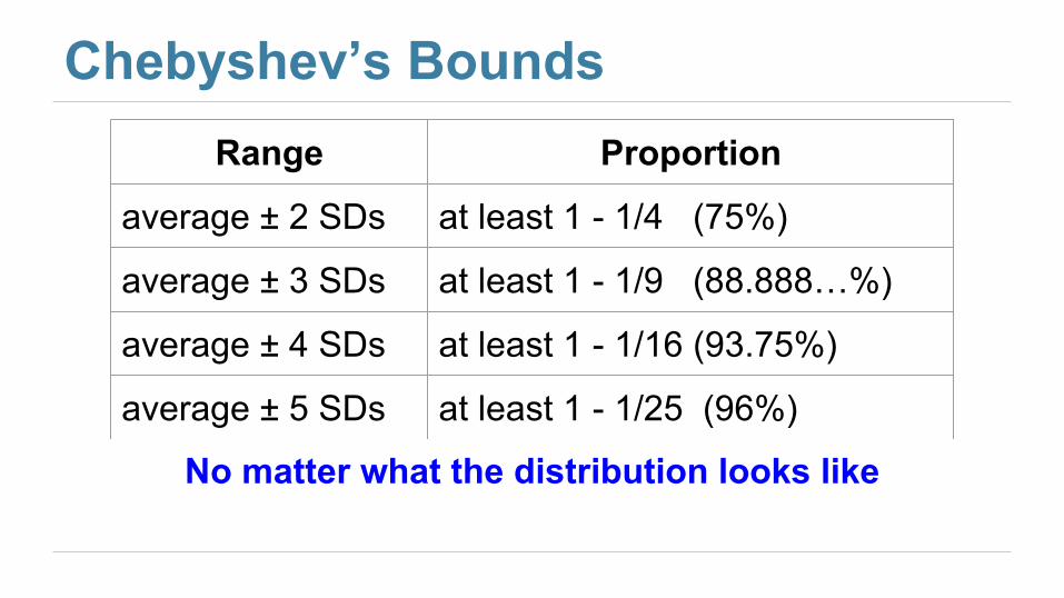
Chebyshev’s BoundsRange Proportion

average ± 2 SDs at least 1 - 1/4 (75%)

average ± 3 SDs at least 1 - 1/9 (88.888…%)

average ± 4 SDs at least 1 - 1/16 (93.75%)

average ± 5 SDs at least 1 - 1/25 (96%)

No matter what the distribution looks like

Standard Units

Standard Units● How many SDs above average?● z = (value - mean)/SD

○ Negative z: value below average○ Positive z: value above average○ z = 0: value equal to average○ Note z=1 implies SD = value-mean

● When values are in standard units: average = 0, SD = 1● Chebyshev: At least 96% of the values of z are between

-5 and 5

Discussion QuestionFind whole numbers that are close to:

(a)the average age

(a)the SD of the ages

The SD and the Histogram

● Usually, it's not easy to estimate the SD by looking at a histogram.

● But if the histogram has a bell shape, then you can.

The SD and Bell-Shaped CurvesIf a histogram is “bell-shaped” then

● the average is at the center

● the range of the data is about ± 3 SDs

● 95% of the data is about ± 2 SDs

(Demo)

The Normal (Gaussian) Distribution

The Standard Normal CurveA very beautiful formula that we won’t use at all -- but you can use it to amazing and impress your friends:

Bell Curve

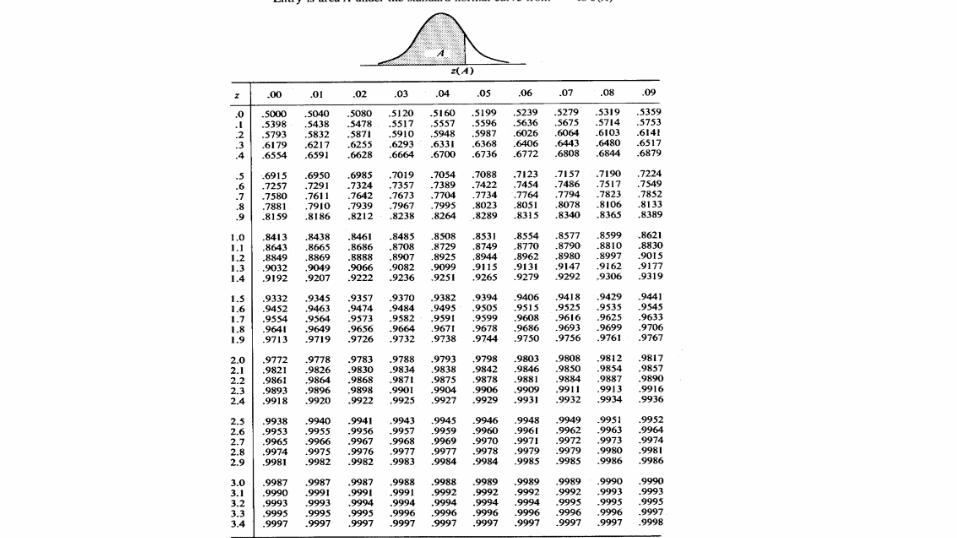
stats.norm.cdf(1)= .8413

(Demo)

1-stats.norm.cdf(1)= .1587

How Big are Most of the Values?No matter what the shape of the distribution (Chebyshev),the bulk of the data are in the range “average ± 5 SDs”

If a histogram is bell-shaped (normal), then● Almost all of the data are in the range

“average ± 3 SDs”

Chebyshev’s BoundsRange Proportion

average ± 2 SDs at least 1 - 1/4 (75%)

average ± 3 SDs at least 1 - 1/9 (88.888…%)

average ± 4 SDs at least 1 - 1/16 (93.75%)

average ± 5 SDs at least 1 - 1/25 (96%)

No matter what the distribution looks like

Bounds and Normal Approximations

A “Central” Area

(Demo)

Probabilities and Standard Units● How does one calculate Prob( VALUE < ##)?● Define Z = (VALUE - mean)/SDCalculate:

Pr { VALUE < ## }= Pr { (VALUE – mean)/SD < (## – mean)/SD }= Pr { Z < (## – mean)/SD }

● When values are in standard units: Average(Z) = 0, SD(Z) = 1

Central Limit Theorem

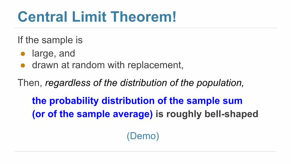
Central Limit Theorem!If the sample is● large, and● drawn at random with replacement,

Then, regardless of the distribution of the population,

the probability distribution of the sample sum (or of the sample average) is roughly bell-shaped

(Demo)

Rouge ou Noir – A bet that the number will be a chosen color

Win $1 for 18 red Lose $1 for 20 non-red

average_per_bet = 1*(18/38) + (-1)*(20/38)= -.05263

American Roulette