Droop models of nutrient-plankton interaction withintratrophic predation

S. R.-J. Jang1, J. Baglama2

1. Department of Mathematics, University of Louisiana at Lafayette, Lafayette,LA 70504-10102. Department of Mathematics, University of Rhode Island, Kingston, RI02881-0816

Abstract. Droop models of nutrient-phytoplankton-zooplankton interactionwith intratrophic predation of zooplankton are introduced and investigated.The models proposed in this study are open ecosystems which include botha constant and a periodic input nutrient models. A simple stochastic modelmimics a randomly varying nutrient input is also presented. For the deter-ministic models it is shown analytically that intratrophic predation has noeffect on the global asymptotic dynamics of the systems if either one of thepopulations has a negative growth rate. Numerical simulations are also usedto investigate the effects of intratrophic predation. Unlike the deterministicmodels for which both populations can coexist with each other if populations’net growth rates are positive, plankton populations can become extinct if theinput nutrient concentration is modeled randomly.

Key words: cell quota – intratrophic predation – uniform persistence –Poincare maps – Wiener process

1 Introduction

Classical deterministic prey-predator models have been exploited to studyand interpret nutrient-plankton interactions very successfully. Intratrophicpredation on the other hand has received only limited attention. Its discus-sion was initiated by Polis [17], who showed that cannibalism is an importantand frequently occurred mechanism in population dynamics. In addition tocannibalism, intratrophic predation may include broader biological phenom-ena. For example, instead of modeling each species under study explicitly to

1

produce a large system, one may build models for which a population con-sisting of several species of organisms and one or more species may prey onothers. This is particularly true for nutrient-plankton interactions as thereare many species of zooplankton and some of the larger species of zooplank-ton do prey on the smaller species.

Kohmeier and Ebenhoh [13] were among the first to propose a mathe-matical model to study intratrophic predation between predator and preyinteraction. The model was extended and analyzed by Pitchford and Brind-ley [16]. Motivated by the consideration of zooplankton, Jang and Baglama[10] proposed a nutrient-phytoplankton-zooplankton model with a constantnutrient input to investigate intratrophic predation. The model was gener-alized to a periodic nutrient input system by Jang et al. [12]. The biologicalconclusions obtained in [10] indicate that intratrophic predation can increasephytoplankton population level and decrease zooplankton population levelfor the coexisting steady state and it can also stabilize the system. For theperiodic input nutrient model [12], it was found that intratrophic predationhas no impact on the asymptotic dynamics of the system if the maximalaverage growth rates of both plankton populations are less than one. More-over, numerical simulations performed in [12] suggest that the mechanismcan eliminate the chaotic behavior of the system.

The above mentioned models assume that growth rate of phytoplank-ton is constantly proportional to its nutrient uptake rate. Consequently, thegrowth rate is directly related to the ambient nutrient available to the pop-ulation. It is known that phytoplankton can uptake nutrient in excess ofits immediate needs. Experiments performed by Ketchum [24] have demon-strated that algae can continue to grow and divide for quite some time evenwhen the ambient nutrient is depleted. Several models have been formulatedto incorporate this observation. Our main objective in this manuscript isto study intratrophic predation by taking this phenomena into considera-tion. Specially, we will use the Droop model [3] developed by Droop to studynutrient-plankton interaction with intratrophic predation.

Following that of [10, 11, 13, 16] we assume that the food resource avail-able to the zooplankton is a weighted sum of phytoplankton and zooplankton.In addition, it is assumed that the nutrient concentration is separated intointernal and external nutrient concentration and only the internal nutrientconcentration is capable of catalyzing cell growth for phytoplankton. Thatis, we adopt the Droop model mechanism for phytoplankton growth [3, 4].Such a model is also refereed to as a variable-yield model.

2

When the input nutrient concentration is a constant, the dynamics of thesystem depend on the maximal growth rates of the plankton populations rel-ative to the total removal rates. Intratrophic predation has no effect on thedynamics of the model if phytoplankton’s net growth rate, i.e., the maximalgrowth rate minus the total removal rate, is negative. The same is true forthe periodic nutrient input model. When the net growth rates of both pop-ulations are positive, numerical techniques are then employed to further ourinvestigation. The simulations suggest that intratrophic predation can elim-inate the chaotic behavior of the system when the input nutrient is modeledperiodically. Unlike the deterministic models for which both populations canpersist when the maximum growth rates of both populations are positive,numerical simulations with the functional forms and parameter values cho-sen suggest that it is possible for both populations to become extinct whena white noise is added to the system.

In the next section, model derivation and analysis for the constant nutri-ent input are presented. Section 3 studies a periodic system with a fluctuatingnutrient input. Numerical simulations are given in section 4. The last sectionprovides a brief summary.

2 A model with constant nutrient input

As usual we let N(t), P (t) and Z(t) denote the nutrient concentration, theconcentrations (or number of cells) of phytoplankton and zooplankton pop-ulation at time t, respectively. Their units are nitrogen or nitrate per unitvolume. It is assumed that the algal cell is capable of storing nutrient. Asa result there is a new state variable, Q(t), the cell quota, which is the av-erage amount of stored nutrient per algal cell at time t. Notice that Q(t) isdimensionless. In this type of models, the growth rate of the phytoplanktondepends on the cell quota, while the uptake rate depends on the ambientnutrient, and possibly also on the cell quota. We let u(Q) and ρ(N, Q)be the per-capita growth rate and per-capita uptake rate of phytoplank-ton, respectively. Motivated by the explicit examples of functions u and ρin the literature [3, 4, 6, 7, 14], we make the following assumptions as in[8, 11, 15, 18, 19, 20].

(H1) There exists Q0 > 0 such that u(Q0) = 0, u′(Q) > 0 and u′(Q) iscontinuous for Q ≥ Q0.

3

(H2) ρ ∈ C1(N, Q) for N ≥ 0, Q ≥ Q0; ρ(0, Q) = 0 for Q ≥ Q0;∂ρ

∂N> 0 and

∂ρ

∂Q≤ 0 for N ≥ 0, Q ≥ Q0.

The quantity Q0 is the minimum cell quota necessary to allow for any celldivision. Parameters δ > 0 and ε > 0 are the death rates of phytoplanktonand zooplankton respectively. The zooplankton’s grazing rate is modeled bya simple linear functional response. Such a simple linear functional responsewas also used in the study of a closed Droop nutrient-plankton model whenthe nutrient is inhibiting [9].

Similar to [10, 12, 13, 16], we assume the food resource that is availableto the zooplankton is P + bZ, where 0 ≤ b ≤ 1 is the intensity of intrat-rophic predation. If b = 0, then phytoplankton is the only food resource forzooplankton. If b = 1, then zooplankton consumes both phytoplankton andits own population indiscriminatly. Since we model nutrient-plankton inter-action in an open ecological system, it is assumed in this section that thereis a constant input nutrient concentration N0 continuously pouring into thesystem with a constant input rate D. Both populations and the nutrientconcentration are also flowing out of the system continuously. For simplicity,it is assumed that the washout rate is a constant and equals to D. Sincethe two plankton populations are modeled in terms of their nutrient contentand there is no nutrient loss due to death or due to nutrient conversion, themodel takes the following form

N = D(N0 −N)− Pρ(N,Q) + δPQ + εZ + m(1− α)PQZ + (1− α)bZ2

P = P [u(Q)− δ −D −mZ]

Q = ρ(N,Q)− u(Q)Q (2.1)

Z = [α(mPQ + bZ)− bZ − ε−D]Z

P (0) ≥ 0, Q(0) ≥ Q0, Z(0) ≥ 0, N(0) ≥ 0,

where m is the maximal zooplankton grazing rate, and α is the zooplanktonconversion rate, 0 < α ≤ 1.

Clearly solutions of system (2.1) exist for all positive time. Also asQ|Q=Q0 ≥ 0, we see that solutions of (2.1) remain nonnegative with Q(t) ≥ Q0

for t > 0. Letting S = N + PQ + Z. Then S = D(N0−S), and we conclude

4

that (2.1) has the following limiting system

P = P [u(Q)− δ −D −mZ]

Q = ρ(N0 − PQ− Z,Q)− u(Q)Q (2.2)

Z = [α(mPQ + bZ)− bZ − ε−D]Z

P (0) ≥ 0, Q(0) ≥ Q0, Z(0) ≥ 0, P (0)Q(0) + Z(0) ≤ N0.

We shall analyze system (2.2) and discuss its dynamical consequence withrespect to the parameter b, the intensity of intratrophic predation.

Let∆ = (P, Q, Z) ∈ R3

+ : Q ≥ Q0, PQ + Z ≤ N0.Then ∆ is positively invariant for (2.2). We first derive the existence condi-tions for steady states. Clearly E0 = (0, Q, 0) always exists, where Q satisfies

ρ(N0, Q) = u(Q)Q.

Steady states of the form (P, Q, 0) on the interior of nonnegative PQ- planesatisfy u(Q) = δ + D and ρ(N0 − PQ, Q) = (δ + D)Q. Thus steady stateE1 = (P1, Q1, 0) exists if and only if u(∞) > δ+D and ρ(N0, Q1) > (δ+D)Q1,where Q1 solves u(Q) = δ + D. Note that in this case Q1 < Q and steadystate E1 is unique if it exists. It can be easily seen that there is no steadystate on the interior of nonnegative PZ or QZ- plane and steady states E0

and E1 do not depend on b. Therefore intratrophic predation has no effecton the existence and magnitude of the boundary steady states. We shall seethat this conclusion in general is not true for the interior steady states.

Indeed, we first consider b = 0 when there is no intratrophic predation.Notice Q0 of steady state E0

2 = (P0, Q0, Z0) must satisfy

ρ(N0 − ε + D

αm− u(Q)− δ −D

m,Q) = u(Q)Q. (2.3)

Let the left hand side of (2.3) be denoted by f(Q). Then f ′(Q) < 0 forQ ≥ Q0 and thus Q0 > 0 exists if and only if

N0 >ε + D

αm− δ + D

m. (2.4)

Hence E02 = (P0, Q0, Z0) exists if and only if (2.4) holds and u(Q0) > δ + D.

In this case Z0 =u(Q0)− δ −D

m, P0 =

ε + D

αmQ0

, Q0 > Q1 and the positive

steady state is unique.

5

When 0 < b ≤ 1, Qb of a positive steady state Eb2 = (Pb, Qb, Zb) must

satisfy

ρ(N0 −ε + D + b(1− α)

u(Q)− δ −D

mαm

− u(Q)− δ −D

m,Q) = u(Q)Q.

Similar to the case for b = 0, the derivative of the left hand side of the aboveequation, denoted by g(Q), with respect to Q, is negative for Q ≥ Q0. HenceEb

2 exists if and only if

N0 >ε + D

αm− b(1− α)(δ + D)

αm2− δ + D

m, (2.5)

and u(Qb) > δ + D. Also Eb2 is unique if it exists, and Qb > Q1.

We proceed to compare the effect of b on the existence and magnitude ofthe positive steady state. Clearly f(Q1) = g(Q1) and the graph of y = g(Q)lies above the graph of y = f(Q) when Q0 ≤ Q < Q1 and below the graphof y = f(Q) when Q > Q1. Since Qb, Q0 > Q1, we see that Qb < Q0 for0 < b ≤ 1. On the other hand it is more likely for (2.5) to occur when b > 0than that of (2.4). Since Qb < Q0, it is more likely that u(Q0) > δ + D thanu(Qb) > δ + D. Therefore intratrophic predation may or may not promotethe existence of the coexisting steady state. However, if the input nutrientconcentration N0 is sufficiently large so that (2.4) holds, then intratrophicpredation can diminish the existence of coexisting steady state as Qb < Q0

and u(Qb) > δ + D is less likely than u(Q0) > δ + D. Furthermore, sinceQb < Q0, we have Zb < Z0 and

Pb =ε + D + b(1− α)

u(Qb)− δ −D

mαmQb

>ε + D

αmQb

>ε + D

αmQ0

= P0.

Thus intratrophic predation can increase phytoplankton population and de-crease zooplankton population of the coexisting steady state (cf. [10]).

Once the mechanism of intratrophic predation is investigated for the ex-istence and magnitude of the steady states of (2.2), we turn to examine itseffect on the stability of these simple solutions. Since lim sup

t→∞N(t) ≤ N0 and

Q ≤ ρ(N0, Q) − u(Q)Q, it follows that lim supt→∞

Q(t) ≤ Q. Therefore Q may

be viewed as the maximum cell quota that a phytoplankton cell can obtain.

6

As a result, both populations go to extinction if the maximal growth rate ofphytoplankton, u(Q), is less than its total removal rate, δ + D, as stated inthe next theorem.

Theorem 2.1 If u(Q) < δ +D, then system (2.2) has only the trivial steadystate E0 = (0, Q, 0) and every solution of (2.2) converges to E0 for 0 ≤ b ≤ 1.

Proof. We first show that E0 is the only steady state for system (2.2). Ifu(Q) = δ+D has a solution Q1, then Q1 > Q. Thus ρ(N0, Q1) ≤ ρ(N0, Q) =u(Q)Q < u(Q1)Q1, which implies that E1 does not exist. Similarly if Eb

2 =(Pb, Qb, Zb) exists for some 0 ≤ b ≤ 1, then Qb > Q. But then ρ(N0 −PbQb − Zb, Qb) < ρ(N0, Qb) ≤ ρ(N0, Q) = u(Q)Q < u(Qb)Qb and we obtaina contradiction. Hence Eb

2 does not exist and E0 is the only steady state forthe system.

It remains to show that E0 is globally asymptotically stable for 0 ≤b ≤ 1. If u(Q) < δ + D for Q ≥ Q0, then P (t) ≤ 0 for t ≥ 0 and thuslimt→∞

P (t) = P ∗ ≥ 0 exists. Since limt→∞

P (t) = 0, we must have P ∗ = 0

and hence limt→∞

P (t)Q(t) = 0 as solutions of (2.2) are bounded. Thus for

any η > 0 there exists t0 ≥ 0 such that P (t)Q(t) < η for t ≥ t0. Wechoose η > 0 such that αmη < ε. Then Z(t) ≤ (αmη − ε)Z for t ≥ t0implies lim

t→∞Z(t) = 0. Therefore for any η > 0 there exists t1 > 0 such that

P (t)Q(t) + Z(t) < η for t ≥ t1. We choose η > 0 such that η < N0. SinceQ(t) ≥ ρ(N0 − η, Q) − u(Q)Q for t ≥ t1, a simple comparison argumentyields lim inf

t→∞Q(t) ≥ Q. Combining this with lim sup

t→∞Q(t) ≤ Q, we have

limt→∞

Q(t) = Q, and solutions of (2.2) converge to E0.

Suppose now u(Q) = δ + D has a solution Q1. We show that Q(t) < Q1

for all t large and this will complete our proof. Suppose on the contrary thatQ(t) ≥ Q1 for t ≥ 0. Then Q ≤ ρ(N0, Q)−u(Q)Q ≤ ρ(N0, Q1)−u(Q1)Q1 <0 as E1 does not exist, which implies lim

t→∞Q(t) = Q∗ ≥ Q1 exists. But then

this contradicts limt→∞

Q(t) = 0. Therefore there must exist t0 ≥ 0 such that

Q(t0) = Q1. Consequently Q(t) < Q1 for t > t0 as Q(t0) < 0.

It follows from the above theorem that intratrophic predation has no im-pact on the global dynamics of the system if u(Q) < δ + D. The inequalityu(Q) < δ + D implies that the maximal growth rate of phytoplankton is lessthan its total removal rate, i.e., phytoplankton’s net growth rate is negative.

7

Therefore phytoplankton population becomes extinct due to insufficient nu-trient concentration available to the population. Consequently, zooplanktonpopulation also becomes extinct and intratrophic predation has no effect onthe dynamics of the system.

Suppose now u(Q) > δ + D. Then u(Q) = δ + D has a solution Q1

and ρ(N0, Q1) ≥ ρ(N0, Q) = u(Q)Q > (δ + D)Q1, which implies steadystate E1 = (P1, Q1, 0) exists and E0 is a saddle point with stable manifoldlying on the QZ-plane. Dynamics of system (2.2) when u(Q) > δ + D and

P1Q1 <ε + D

αmcan be summarized below.

Theorem 2.2 Let u(Q) > δ + D and P1Q1 <ε + D

αm. Then E0 = (0, Q, 0)

and E1 = (P1, Q1, 0) are the only steady states for system (2.2). In addition

ρ(N0 − ε + D

αm,Q0) < (δ + D)Q0 if N0 >

ε + D

αm, then solutions of (2.2) with

P (0) > 0 converge to E1 for 0 ≤ b ≤ 1.

Proof. If Eb2 = (Pb, Qb, Zb) exists for some 0 ≤ b ≤ 1, then it follows from

the second equation of (2.2) that PbQb < P1Q1. But since

PbQb =ε + D + bZb − αbZb

αm>

ε + D

αm> P1Q1,

we obtain a contradiction. Thus Eb2 does not exist for any b, 0 ≤ b ≤ 1.

Since the positive PQ- plane is positively invariant and∂P

∂P+

∂Q

∂Q= −δ −

D− P∂ρ

∂N+

∂ρ

∂Q− u′(Q)Q < 0 for P > 0, Q ≥ Q0, it follows from the Dulac

criterion that E1 is globally asymptotically stable on the positive PQ- plane.We show that lim

t→∞Z(t) = 0 for any solution (P (t), Q(t), Z(t)) of (2.2)

with P (0) > 0. This is trivially true if Z(0) = 0. Let Z(0) > 0. Then

Z(t) > 0 for t ≥ 0. If N0 ≤ ε + D

αm, then Z ≤ (αmN0 − ε−D)Z ≤ 0 implies

limt→∞

Z(t) = 0. Suppose now N0 >ε + D

αm. If P (t)Q(t) >

ε + D

αmfor t ≥ 0,

8

then by our assumption

˙(PQ)(t) = −(δ + D)PQ−mPQZ + Pρ(N0 − PQ− Z,Q)

≤ P [ρ(N0 − PQ, Q)− (δ + D)Q]

< P [ρ(N0 − ε + D

αm,Q0)− (δ + D)Q0]

< 0

implies limt→∞

P (t)Q(t) = A exists where 0 < A < ∞. But since A ≥ ε + D

αm

and ρ(N0 − ε + D

αm,Q0) < (δ + D)Q0, it contradicts to lim

t→∞˙(PQ) = 0.

Therefore there must exist t0 ≥ 0 such that (PQ)(t0) =ε + D

αm. But then

˙(PQ)(t0) < 0 and thus (PQ)(t) <ε + D

αmfor all t large. Consequently

Z(t) ≤ 0 for all t large and limt→∞

Z(t) = z∗ ≥ 0 exists. Using the fact that

limt→∞

Z(t) = 0, we have z∗ = 0. As a result, the ω-limit set lies on the positive

PQ-plane and E1 is globally asymptotically stable on the indicated region.

We conclude from Theorem 2.2 that intratrophic predation has no ef-fect on the asymptotic dynamics of the system if u(Q) > (δ + D) and

P1Q1 <ε + D

αm. Note that αmP1Q1 is the maximal growth rate of zoo-

plankton when phytoplankton population is stabilized at the steady stateE1. Consequently, αmP1Q1− (ε + D) is the net growth rate of zooplankton.Intratrophic predation has no influence on the system if zooplankton’s netgrowth rate is negative when phytoplankton’s net growth rate is positive.The case when both populations’ net growth rate is positive is summarizedbelow.

Theorem 2.3 Let u(Q) > (δ + D) and P1Q1 >ε + D

αm. Then Eb

2 =

(Pb, Qb, Zb) exists for 0 ≤ b ≤ 1. Moreover,

(a) System (2.2) is uniformly persistent for 0 ≤ b ≤ 1.

(b) Pb > P0 and Zb < Z0 for any b, 0 < b ≤ 1.

9

Proof. Since P1Q1 >ε + D

αm, N0 ≥ P1Q1 >

ε + D

αm>

ε + D

αm− δ + D

m. Thus

if E02 does not exist we must have u(Q0) ≤ (δ + D), where Q0 satisfies (2.3).

Hence

ρ(N0 − ε + D

αm, Q0) ≤ ρ(N0 − ε + D

αm− u(Q0)− δ −D

m, Q0)

= u(Q0)Q0 ≤ u(Q1)Q1 = ρ(N0 − P1Q1, Q1)

and thus

ρ(N0 − ε + D

αm,Q1) ≤ ρ(N0 − ε + D

αm, Q0) ≤ ρ(N0 − P1Q1, Q1),

which yields P1Q1 ≤ ε + D

αmand contradicts our assumption. This shows

that E02 exists. Similar arguments imply that Eb

2 exists for 0 < b ≤ 1. Theproof of (b) follows from an earlier analysis. To show (a), observe that thesystem is weakly persistent by the Jacobian matrix evaluated at E0 and E1

[5], and thus uniformly persistent by [21] as the system is dissipative.

The above analysis was carried out on the limiting system (2.2). As in [10]we can make the same conclusion for the original system (2.1) by applyingthe asymptotic autonomous arguments derived by Thieme [21].

3 A model with periodic nutrient input

In this section we shall relax the assumption made in the previous section thatthe input nutrient concentration is a constant. To incorporate day/night orseasonal variations of the nutrient in a natural environment, we assume thatthe input concentration of the limiting nutrient varies periodically around amean value N0 > 0, with an amplitude a, 0 < a < N0, and period τ . That is,according to the law N0 + ae(t), where e(t) is a τ -periodic function of mean

value zero and |e(t)| ≤ 1. We denote by 〈h(t)〉 =1

τ

∫ τ

0

h(t)dt the mean value

of a τ -periodic function h.

10

Model (2.1) with a fluctuating nutrient input takes the following form.

N = D(N0 + ae(t)−N)− Pρ(N,Q) + δPQ + m(1− α)PQZ + εZ

+(1− α)bZ2

P = P [u(Q)− δ −D −mZ]

Q = ρ(N,Q)− u(Q)Q (3.1)

Z = [α(mPQ + bZ)− bZ − ε−D]Z

N(0) ≥ 0, P (0) ≥ 0, Q(0) ≥ Q0, Z(0) ≥ 0.

The parameters appeared in (3.1) are defined as in section 2. Similar to [8],we begin by considering the τ -periodic equation

N = D(N0 + ae(t)−N). (3.2)

Notice that (3.2) has a unique positive τ -periodic solution N∗(t) and everysolution N(t) of (3.2) satisfies lim

t→∞(N(t) − N∗(t)) = 0, where N0 − a ≤

N∗(t) ≤ N0 + a for t ≥ 0.We let S = N∗(t) − N − PQ − Z and notice that S = −DS. As a

result limt→∞

(N(t) + P (t)Q(t) + Z(t)−N∗(t)) = 0, and system (3.1) has the

following limiting system

P = P [u(Q)− δ −D −mZ]

Q = ρ(N∗(t)− PQ− Z, Q)− u(Q)Q (3.3)

Z = [α(mPQ + bZ)− bZ − ε−D]Z

P (0) ≥ 0, Q(0) ≥ Q0, P (0)Q(0) + Z(0) ≤ N∗(0).

It can be easily verified that solutions of (3.3) satisfy P (t) ≥ 0, Q(t) ≥Q0, Z(t) ≥ 0, P (t)Q(t) + Z(t) ≤ N∗(t) for t ≥ 0, and system (3.3) is dissipa-tive. Several variable-yield models with periodic nutrient input were studiedin [11, 20]. Our analysis presented here is similar to that of [11].

LetΓ = (P,Q, Z) ∈ R3

+ : Q ≥ Q0, PQ + Z ≤ N∗(0).Since (3.3) is τ -periodic, we shall consider the Poincare map P induced by(3.3), where P : Γ → Γ is defined by P(P (0), Q(0), Z(0)) = (P (τ), Q(τ), Z(τ)),and (P (t), Q(t), Z(t)) is the solution of (3.3) with initial condition (P (0), Q(0), Z(0)).Since (3.3) is dissipative, P has a global attractor K, i.e., K is the maximalcompact invariant set such that lim

n→∞Pnx ∈ K for any x ∈ Γ.

11

Consider the following trivial τ -periodic equation

q = ρ(N∗(t), q)− u(q)q, (3.4)

q(0) ≥ Q0.

Notice that (3.4) has a unique τ -periodic solution Q∗(t) which is moreoverglobally asymptotically attracting for (3.4) by [20]. Consequently, (3.3) al-ways has a trivial τ -periodic solution (0, Q∗(t), 0), although Q∗(t) is biologi-cally irrelevant as there is no phytoplankton present.

Theorem 3.1 If 〈u(Q∗(t))〉 < δ + D, then limt→∞

P (t) = limt→∞

Z(t) = 0 and

limt→∞

(Q(t)−Q∗(t)) = 0 for any solution of (3.3) and 0 ≤ b ≤ 1.

Proof. Since Q ≤ ρ(N∗(t), Q)−u(Q)Q, we have Q(t) ≤ q(t) for t ≥ 0, whereq(t) is the solution of (3.4) with q(0) = Q(0). Furthermore, q(t)−Q∗(t) → 0as t →∞, we have for all t sufficiently large that

P (t + τ) ≤ P (t)eτ/2〈u(Q∗(t))− δ −D〉.

Thus limt→∞

P (t) = 0 by our assumption, and limt→∞

P (t)Q(t) = 0 as solutions of

(3.3) are bounded. Therefore it can be proved that limt→∞

Z(t) = 0.

It remains to show limt→∞

(Q(t)−Q∗(t)) = 0. Notice that the global attractor

K of the Poincare map P lies on the Q-axis as limt→∞

P (t) = limt→∞

Z(t) = 0.

Restricted to the Q-axis, Pn(0, Q(0), 0) = (0,Pn1 (Q(0)), 0), where P1 is the

Poincare map induced by (3.4). Since Q∗(0) is the unique fixed point of P1

which is moreover globally asymptotically stable for P1, it follows that P hasa unique fixed point (0, Q∗(0), 0) which is globally asymptotically stable forP . Therefore the trivial τ -periodic solution (0, Q∗(t), 0) is globally attractingfor (3.3) and this completes the proof.

Since N∗(t) is the maximum external nutrient concentration available tothe system at any time t, < u(Q∗(t)) > can be viewed as the average maximalgrowth rate of phytoplankton. Both populations go to extinction if the netgrowth rate of phytoplankton is negative, i.e., if < u(Q∗(t)) >< δ + D.Consequently, intratrophic predation has no effect on the global dynamics ofthe limiting system if phytoplankton has a negative net growth rate.

Since the nonnegative PQ-plane is positively invariant, we consider the

12

PQ-subsystem of (3.4)

P = P [u(Q)− δ −D],

Q = ρ(N∗(t)− PQ, Q)− u(Q)Q, (3.5)

Q(0) ≥ Q0, P (0) ≥ 0, P (0)Q(0) ≤ N∗(0).

By introducing a new state variable, (3.5) was transformed into a com-petitive system for which the dynamics were easily understood. Indeed,if 〈u(Q∗(t))〉 > δ + D, then system (3.5) has a unique τ -periodic solution(P (t), Q(t)) with P (t) > 0 and Q(t) > Q0. Moreover, solution (P (t), Q(t))of (3.5) with P (0) > 0 all converge to (P (t), Q(t)) [20]. It follows thatsystem (3.3) has a unique τ -periodic solution of the form (P (t), Q(t), 0) if〈u(Q∗(t))〉 > δ + D, where P (t) > 0 and Q(t) > Q0. Since 〈N∗(t)〉 is themaximum average nutrient concentration available in the system, we havethe following immediate consequence.

Theorem 3.2 If 〈u(Q∗(t))〉 > δ + D and αm〈N∗(t)〉 < ε + D, then solution(P (t), Q(t), Z(t)) of (3.3) with P (0) > 0 converges to (P (t), Q(t), 0) as t →∞ for 0 ≤ b ≤ 1.

Proof. As in [11] we consider the Poincare map P : Γ → Γ induced by sys-tem (3.3). By the assumption αm〈N∗(t)〉 < ε + D, we have lim

t→∞Z(t) = 0

and the global attractor K of P lies on the PQ-plane. Restricted to this set,Pn(P (0), Q(0), 0) = (Sn(P (0), Q(0)), 0), where S is the Poincare map associ-ated with system (3.5). It follows that P has two fixed points (0, Q∗(0), 0) and(P (0), Q(0), 0). We shall show that lim

n→∞Pn(P (0), Q(0), Z(0)) = (P (0), Q(0), 0)

if P (0) > 0. To this end, let A = (P,Q, Z) ∈ Γ : P = 0 be a closed subsetof Γ. Our assumption implies that the maximal compact invariant subset ofA is M = (0, Q∗(0), 0) which is moreover isolated in the PQ-plane. TheJacobian derivative D(P) of P at (0, Q∗(0), 0) is given by Φ(τ), where Φ(t)is the fundamental matrix solution of X = B(t)X with

B(t) =

u(Q∗(t))− δ −D 0 0

−Q∗(t) ∂ρ∂N

∂ρ∂Q− u′(Q∗(t))Q∗(t)− u(Q∗(t)) − ∂ρ

∂N

0 0 −ε−D

.

It follows from B(t) that the stable set W s(M) of M , x ∈ Γ : limn→∞

Pnx ∈M, lies on A. Therefore, P is uniformly persistent with respect to A by[25], i.e., there exists η > 0 such that lim inf

n→∞d(Pn(P (0), Q(0), Z(0)), A) > η

13

for any (P (0), Q(0), Z(0)) ∈ Γ with P (0) > 0. Consequently, the ω-limit setof P has the form (P, Q, 0) with P > η. Therefore, Pn(P (0), Q(0), Z(0)) →(P (0), Q(0), 0) as n →∞ if P (0) > 0 and the assertion follows.

We conclude from Theorem 3.2 that intratrophic predation has no effecton the global asymptotic dynamics of the limiting system if phytoplankton’snet growth rate is positive but zooplankton has a negative net growth rate.By using periodic solutions (0, Q∗(t), 0) and (P (t), Q(t), 0) and their associ-ated Floquet multipliers, we obtain a sufficient condition for the persistenceof both populations on the ω-limit set of system (3.1) as given below.

Theorem 3.3 If 〈u(Q∗(t))〉 > δ + D and αm〈P (t))Q(t)〉 > ε + D, thensystem (3.3) is uniformly persistent and has a positive τ -periodic solution(P 0

b (t), Q0b(t), Z

0b (t)), where P 0

b (t), Z0b (t) > 0 and Q0

b(t) > Q0 for 0 ≤ b ≤ 1.

Proof. As 〈u(Q∗(t))〉 > δ + D, the τ -periodic solution (P (t), Q(t), 0) exists.Similar to [11], we apply Theorem 3.1 of Butler and Waltman [?] to showuniform persistence of (3.3). Let F be the continuous semiflow generatedby (3.3) and ∂F be F restricted to the boundary ∂Γ. It is easy to verifythat ∂F is isolated and acyclic. Indeed, let M0 = (0, Q∗(t), 0)|0 ≤ t ≤ τ,M1 = (P (t), Q(t), 0)|0 ≤ t ≤ τ , and let ω(x) denote the ω-limit set of x.Then the invariant set of ∂F , Ω(∂F) = ∪x∈∂Γω(x), is M0,M1. Clearly ∂Fis acyclic as M0 and M1 are globally attracting on the positive Q-axis, and thepositive PQ-plane, respectively so that no subset of M0,M1 forms a cycle.It remains to show that each Mi is isolated for ∂F and for F respectively, fori = 0, 1. We only prove that M0 is isolated for F as the remaining assertioncan be shown similarly.

Since 〈u(Q∗(t))〉 > δ + D, we can choose ρ > 0 such that

1/τ

∫ τ

0

[u(Q∗(t)− ρ)− (δ + D + mρ)]dt > 0. (3.6)

Let N = (P,Q, Z) ∈ Γ : d((P, Q,Z), M0) < ρ, where d denotes the Eu-clidean metric on R3. We show that N is an isolating neighborhood of M0

in Γ, i.e., M0 is the maximal invariant set in N . If not, then there ex-ists an invariant set V in Γ such that M0 ⊂ V ⊂ N and V \ M0 6= ∅.Since M1 is globally attracting in the positive PQ-plane, there exists x(0) =(P (0), Q(0), Z(0)) ∈ V \M0 such that P (0), Z(0) > 0 and x(t) ∈ V for all t.

14

But V ⊂ N implies

P

P= u(Q)− δ −D −mZ

≥ u(Q∗(t)− ρ)− δ −D −mρ

and thus limt→∞

P (t) = ∞ by (3.6). We obtain a contradiction and conclude

that M0 is isolated for F . LetΓ denote the interior of Γ. It follows from the

Floquet multipliers of the τ -periodic solutions (0, Q∗(t), 0) and (P (t), Q(t), 0)

that W s(Mi)∩Γ= ∅ for i = 0, 1, where W s(Mi) denotes the stable set of Mi.

Therefore, we can conclude that (3.3) is uniformly persistent by Theorem 3.1of [?]. Furthermore, since the system is dissipative and uniformly persistent,the interior of Γ has a τ -periodic solution by Theorem 4.11 of [26]. Thus(3.4) has a positive τ -periodic solution for 0 ≤ b ≤ 1 and this completes theproof.

Once the dynamics of system (3.3) are well understood, we can apply thesame technique used in [12] to conclude that systems (3.1) and (3.3) havethe same asymptotic dynamics. Therefore, intratrophic predation may haveimpact on the model only if the maximum average net growth rates of bothplankton populations are positive. However, unlike the autonomous systemfor which comparison of magnitude between interior steady states can beeasily made, it is not clear for the interior periodic solutions presented here.We will rely mainly on numerical simulations given in the next section tomake such further comparison.

4 Numerical simulations

It was shown analytically in the previous sections that intratrophic predationhas no impact on the dynamics of the systems if population’s net growthrate is negative. In this section we will use numerical examples to studythe mechanism when both population’s net growth rate is positive. We usethe growth rate u and uptake rate ρ proposed by Grover in his experimentalstudy [6, 7] to simulate our models (cf. [11]). Specifically,

u(Q) = umax(Q−Qmin)+

k + (Q−Qmin)+

,

15

ρ(N, Q) = ρmax(Q)N

N + 4,

where ρmax(Q) = ρhighmax−(ρhigh

max−ρlowmax)

(Q−Qmin)+

Qmax −Qmin

and (Q−Qmin)+ denotes

the positive part of Q−Qmin. Specific parameter values are ρhighmax = 15, ρlow

max =0.9, Qmin = 3, Qmax = 30, umax = 2.16 and k = 2. From Qmin = 3, we seethat Q0 = 3. These parameter values are within the wide range studied byGrover [6, p. 817].

The zooplankton’s grazing rate is modeled by a simple linear functionmP , and we choose m = 5 for our simulations. A linear functional formwas also used in the study of nutrient-plankton interaction with a limitingnutrient inhibiting the growth rate of phytoplankton [8]. Limiting system(2.3) with the above functional forms becomes

P = P [2.16(Q− 3)+

2 + (Q− 3)+

− δ −D − 0.5Z]

Q = [15− 0.522(Q− 3)+]N0 − PQ− Z

N0 − PQ− Z + 4− 2.16

(Q− 3)+Q

2 + (Q− 3)+

(4.1)

Z = [α(0.5PQ + bZ)− bZ − ε−D]Z

P (0) ≥ 0, Q(0) ≥ 3, Z(0) ≥ 0, P (0)Q(0) + Z(0) ≤ N0.

We use the same death rates δ = 0.7 and ε = 0.1 as in [22, 23] to simulatemodel (4.1). Since we are more interested in the dynamics of the systemwhen both populations can coexist, we choose N0 = 4.85 and D = 0.4so that conditions in Theorem 2.3 are true. Specifically u(Q) = 1.2629 >

δ+D = 1.1, P1 = 0.4079, Q1 = 5.0755 and P1Q1 = 2.0703 >ε + D

αm= 1. For

the functional forms and parameters chosen, the autonomous system, model(4.1), has no periodic solutions for 0 ≤ b ≤ 1. Figure 1 plots components ofthe interior steady state as a function of b. It demonstrates that intratrophicpredation can increase phytoplankton population and decrease zooplanktonpopulation levels of the interior steady state (cf. [10]) as shown in section 2.

Put figure 1 here

For periodic nutrient input model we use N0 = 4.85 as given above,and choose a = 3 and e(t) = sin(π/10t). This particular functional form

16

was also used in the study of intratrophic predation for a constant-yieldperiodic nutrient-plankton system ([12]). In particular, the period is 20 forthe example given. We calculate N∗(t) analytically. The limiting system(3.4) now takes the following form.

P = P [2.16(Q− 3)+

2 + (Q− 3)+

− δ −D − 0.5Z]

Q = [15− 0.522(Q− 3)+]N∗(t)− PQ− Z

N∗(t)− PQ− Z + 4− 2.16

(Q− 3)+Q

2 + (Q− 3)+

(4.2)

Z = [α(0.5)PQ + bZ)− bZ − ε−D]Z

P (0) ≥ 0, Q(0) ≥ 3, Z(0) ≥ 0, P (0)Q(0) + Z(0) ≤ N∗(0).

We use the same parameter values as in the constant nutrient input model.With these parameters, conditions given in Theorem 3.3 are satisfied. There-fore, the corresponding full system is uniformly persistent and has a positiveperiodic solution. Figure 2 plots trajectories (N(t), P (t), Z(t)) with two slightdifferent initial conditions: (N(0), P (0), Q(0), Z(0)) = (1.25, 0.5, 3.5, 1), and(N(0), P (0), Q(0), Z(0)) = (1.26, 0.51, 3.51, 1.01) when b = 0. It is clear thatboth solutions are aperiodic and moreover the system is sensitive to initialconditions. Therefore the interaction between nutrient and plankton popula-tions without intratrophic predation seems chaotic. However, this is not truewhen b = 1 as shown in Figure 3. System (4.2) now has a locally asymptoti-cally attracting positive periodic solution when b = 1. A bifurcation diagramusing b as the bifurcation parameter is presented in Figure 4. The diagramplots 25 maximum phytoplankton population levels after transient behav-ior has been eliminated. From these figures we conclude that intratrophicpredation can stabilize the system.

Put figures 2, 3 and 4 here

Since the input nutrient concentration may vary randomly in the naturalsystem, we next add an environmental noise to system (4.1) as given below.

17

N = D(N0 −N) + cdW (t)

dt− Pρ(N, Q) + δPQ + εZ + m(1− α)PQZ + (1− α)bZ2

P = P [u(Q)− δ −D −mZ]

Q = ρ(N,Q)− u(Q)Q (4.3)

Z = [α(mPQ + bZ)− bZ − ε−D]Z

P (0) ≥ 0, Q(0) ≥ Q0, Z(0) ≥ 0, N(0) ≥ 0,

where W (t), t ∈ [0,∞), is a Wiener process denoting the white noise. Inparticular, probW (0) = 0 = 1, the increment W (t1) −W (t0) is normallydistributed with mean zero and variance t1 − t0, and the increment onlydepends on the length of the time interval but not on any specific time.System (4.3) satisfies the existence and uniqueness conditions given in [].However, we do not study the asymptotic behavior of (4.3) as we did for thedeterministic systems. We use a first order Euler approximation to simulatethe model.

Ni+1 = Ni + D(N0 −Ni)∆t + cηi

√∆t− Piρ(Ni, Qi)∆t + δPiQi∆t + εZi∆t

+ m(1− α)PiQiZi∆t + (1− α)bZ2i ∆t

Pi+1 = Pi + Pi[u(Qi)− δ −D −mZi]∆t (4.4)

Qi+1 = Qi + ρ(Ni, Qi)∆t− u(Qi)Qi∆t

Zi+1 = Zi + [α(mPiQi + bZi)− bZi − ε−D]Zi∆t

N0, P0, Z0 ≥ 0, Q0 ≥ 3,

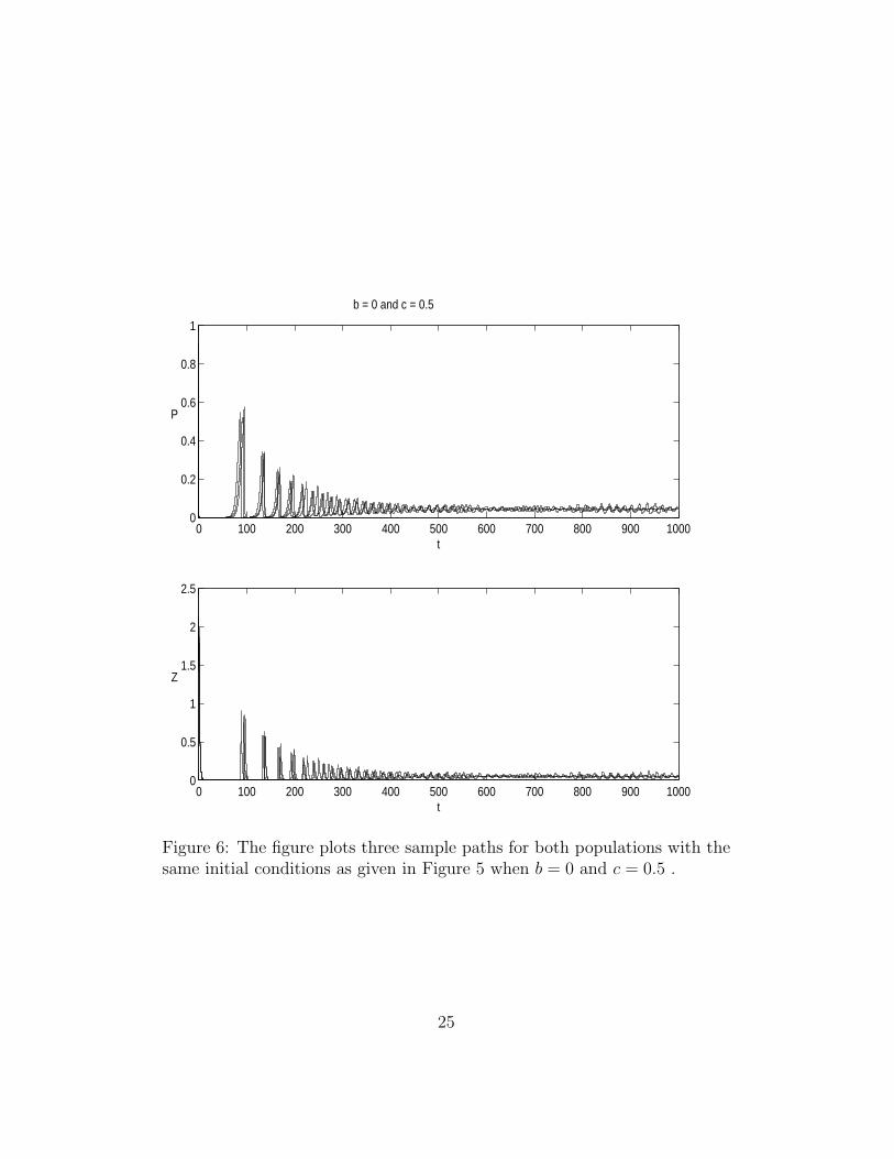
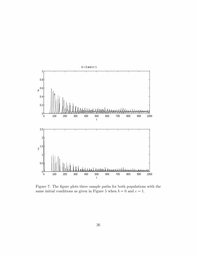
where ηi has a standard normal distribution, i.e., ηi ∼ N(0, 1).We use step size ∆t = 0.01 for all simulations. Figures 5-7 plots 3 sample

paths of the system when b = 0 and c = 0.1, c = 0.5 and c = 1, respectively.The initial condition for each sample path is (1.25, 0.5, 3.5, 1.0) for all sim-ulations. Figures 8 and 9 plot 3 sample paths for system (4.4) for b = 0.1,and b = 0.5 with c = 0.1, respectively. From these figures we see that pop-ulations may go to extinction even when both populations net growth ratesare positive.

18

0 0.1 0.2 0.3 0.4 0.5 0.6 0.7 0.8 0.9 10.18

0.185

0.19

S.S

. P

Co

mp

.

0 0.1 0.2 0.3 0.4 0.5 0.6 0.7 0.8 0.9 15.52

5.525

5.53

5.535

5.54

S.S

. Q

Com

p.

0 0.1 0.2 0.3 0.4 0.5 0.6 0.7 0.8 0.9 10.021

0.0212

0.0214

0.0216

S.S

. Z

Co

mp

.

b

Figure 1: The P -component of the interior steady state increases while theZ-component decreases as b increases.

19

0 200 400 600 800 1000 1200 1400 1600 1800 20000

0.5

1

P

0 200 400 600 800 1000 1200 1400 1600 1800 20003

4

5

6

7

Q

0 200 400 600 800 1000 1200 1400 1600 1800 20000

0.5

1

1.5

2

Z

t

b = 0

Figure 2: The plot for two solutions of system (4.2) with a slight change ofinitial conditions by adding 0.01 to each component. The system exhibitsaperiodic solutions and is sensitive dependent on initial conditions.

20

0 200 400 600 800 1000 1200 1400 1600 1800 20000

0.2

0.4

0.6

0.8

P

0 200 400 600 800 1000 1200 1400 1600 1800 20003

4

5

6

7

Q

0 200 400 600 800 1000 1200 1400 1600 1800 20000

0.5

1

1.5

2

Z

t

b = 1

Figure 3: The chaotic behavior found when b = 0 disappears when b = 1.The positive periodic solution is locally asymptotically stable.

21

0 0.1 0.2 0.3 0.4 0.5 0.6 0.7 0.8 0.9 10

0.1

0.2

0.3

0.4

0.5

0.6

0.7

Pmax

b

Figure 4: The diagram plots 25 maximum phytoplankton population levelsof model (4.2) after the transient behavior has been eliminated.

22

0 100 200 300 400 500 600 700 800 900 10000

0.2

0.4

0.6

0.8

P

t

0 100 200 300 400 500 600 700 800 900 10000

0.5

1

1.5

2

2.5

Z

t

b = 0 and c= 0.1

Figure 5: The figure plots three sample paths for both plankton populationswhen b = 0 and c = 0.1 with the same initial condition. One sample path ofzooplankton population goes extinct.

23

5 Discussion

Several nutrient-phytoplankton-zooplankton models are proposed to investi-gate intratrophic predation. The predator population is consisted of severaldifferent species of zooplankton and some of the species may consume its ownpopulation. Our analytical results for the deterministic models obtained inthis study are similar to those found in [10, 12]. Specifically, intratrophic pre-dation has no impact on the global asymptotic dynamics of both the constantand periodic input nutrient models when the population’s net growth rateis negative. When net growth rates of both populations are positive, it wasshown that intratrophic predation can increase the phytoplankton popula-tion level and decrease zooplankton population level for the coexisting steadystate when the input nutrient is modeled constantly. No such a conclusioncan be achieved for the periodic input nutrient model. However, simulationsperformed in this study suggests that intratrophic predation can eliminatethe chaotic behavior of the system even when the degree of intratrophic pre-dation is very small.

A simple stochastic model simulates a randomly varying nutrient inputwas also proposed in this study. Although the system possesses a unique solu-tion, we do not study its asymptotic dynamics as we did for the deterministicsystems. A first Euler method was used to approximate the solutions. It isfound numerically that both populations may go to extinction even whenthe population’s net growth rates are positive. Therefore, the interactionbetween the plankton populations with intratrophic predation may be muchmore complicated and unpredictable.

24

0 100 200 300 400 500 600 700 800 900 10000

0.2

0.4

0.6

0.8

1

P

t

0 100 200 300 400 500 600 700 800 900 10000

0.5

1

1.5

2

2.5

Z

t

b = 0 and c = 0.5

Figure 6: The figure plots three sample paths for both populations with thesame initial conditions as given in Figure 5 when b = 0 and c = 0.5 .

25

0 100 200 300 400 500 600 700 800 900 10000

0.2

0.4

0.6

0.8

1

P

t

0 100 200 300 400 500 600 700 800 900 10000

0.5

1

1.5

2

2.5

Z

t

b = 0 and c= 1

Figure 7: The figure plots three sample paths for both populations with thesame initial conditions as given in Figure 5 when b = 0 and c = 1.

26

0 100 200 300 400 500 600 700 800 900 10000

0.2

0.4

0.6

0.8

1

P

t

0 100 200 300 400 500 600 700 800 900 10000

0.5

1

1.5

2

2.5

Z

t

b = 0.1 and c= 0.1

Figure 8: The figure plots three sample paths for both populations with thesame initial conditions as given in Figure 5 when b = 0.1 and c = 0.1.

27

0 100 200 300 400 500 600 700 800 900 10000

0.2

0.4

0.6

0.8

P

t

0 100 200 300 400 500 600 700 800 900 10000

0.5

1

1.5

2

2.5

Z

t

b= 0.5 and c= 0.1

Figure 9: The figure plots three sample paths for both populations with thesame initial conditions as given in Figure 5 when b = 0.5 and c = 0.1.

28

References

[1] Busenberg, S., Kumar, S.K., Austin, P., Wake, G.: The dynamics of amodel of a plankton-nutrient interaction. Bull. Math. Biol. 52, 677-696(1990)

[2] DeAngelis, D.L.: Dynamics of Nutrient Cycling and Food Webs. NewYork: Chapman & Hall 1992

[3] Droop, M.R.: Some thoughts on nutrient limitation in algae. J. Phycol-ogy 9, 264-272 (1973)

[4] Droop, M.R.: The nutrient status of algae cells in continuous culture.J. Marine Biol. Asso. U.K. 54, 825-855 (1974)

[5] Freedman, H.I., Waltman, P.: Persistence in models of three interactingpredator-prey populations. Math. Biosci. 68, 213-231 (1984)

[6] Grover, J.P.: Resource competition in a variable environment-phytoplankton growing according to the variable-internal-stores model.Am. Nat. 138, 811-835 (1991)

[7] Grover, J.P.: Constant- and variable-yield models of population growth-Responses to environmental variability and implications for competition.J. Theoret. Biol. 158, 409-428 (1992)

[8] Jang, S.: Dynamics of variable-yield nutrient-phytoplankton-zooplankton models with nutrient recycling and self-shading. J. Math.Biol. 40, 229-250 (2000)

[9] Jang, S., Baglama, J.: Qualitative behavior of a variable-yield simplefood chain with an inhibiting nutrient. Math. Biosci. 164, 65-80 (2000)

[10] Jang, S., Baglama, J., A nutrient-predator-prey model with intratrophicpredation. Appl. Math. Comput. 129, 517-536 (2002).

[11] Jang, S., Baglama, J., Persistence in variable-yield nutrient-planktonmodels. Math. Compu. Mod. 38, 281-298 (2003).

[12] Jang, S., Baglama, J., P. Seshaiyer, Intratrophic predation in a simplefood chain with fluctuating nutrient. Discr. Cont. Dyn. Sys., Ser. B, toappear.

29

[13] Kohlmeier, C., Ebenhoh, W., The stabilizing role of cannibalism in apredator-prey system. Bull. Math. Biol. 57, 401-411 (1995)

[14] Lange, K., Oyarzun, F.J.: The attractiveness of the Droop equations.Math. Biol. 111, 261-278 (1992)

[15] Oyarzun, F.J., Lange, K.: The attractiveness of the Droop equationsII. Generic uptake and growth functions. Math. Biosci. 121, 127-139(1994)

[16] Pitchford, J., Brindley, J., Intratrophic predation in simple predator-predy models. Bull. Math. Biol. 60, 937-953 (1998)

[17] Polis, G.A., The evolution and dynamics of intratrophic predation. Ann.Rev. Ecol. Syst. 12, 225-251 (1981)

[18] Smith, H.L., Waltman, P.: Competition for a single limiting resourcein continuous culture: The variable-yield model. SIAM Appl. Math. 54,1113-1131 (1994)

[19] Smith, H.L., Waltman, P.: The Theory of the Chemostat. New York:Cambridge University Press 1995

[20] Smith, H.L.: The periodically forced Droop model for phytoplanktongrowth in a chemostat. J. Math. Biol. 35, 545-556 (1997)

[21] Thieme, H.R.: Persistence under relaxed point-dissipativity (with appli-cation to an endemic model). SIAM J. Math. Anal. 24: 407-435 (1993)

[22] Ruan, S.: Persistence and coexistence in zooplankton-phytoplankton-nutrient models with instantaneous nutrient recycling. J. Math. Biol.31, 633-654, 1993.

[23] Ruan, S.: Oscillations in plankton models with nutrient recycling. J.Theor. Biol. 208, 15-26, 2001.

[24] Ketchum, B.H.: The absorption of phosphate and nitrate by illuminatedcultures of Nitzchia Closterium. Amer. J. Botany 26, 399-407, 1939.

bibitemthieme Thieme, H.R.: Convergence results and a Poincare-Bendixson trichotomy for asymptotically autonomous differential equa-tions. J. Math. Biol. 30, 755-763, 1992.

30

[25] Hofbauer, J., So, J.W.-H.: Uniform persistence and repellors for maps.Proc. Amer. Math. Soc. 107, 1137-1142 (1989)

[26] Yang, F., Freedman, H.I.: Competing predators for a prey in a chemo-stat model with periodic nutrient input. J. Math. Biol. 29, 715-732,1991.

31