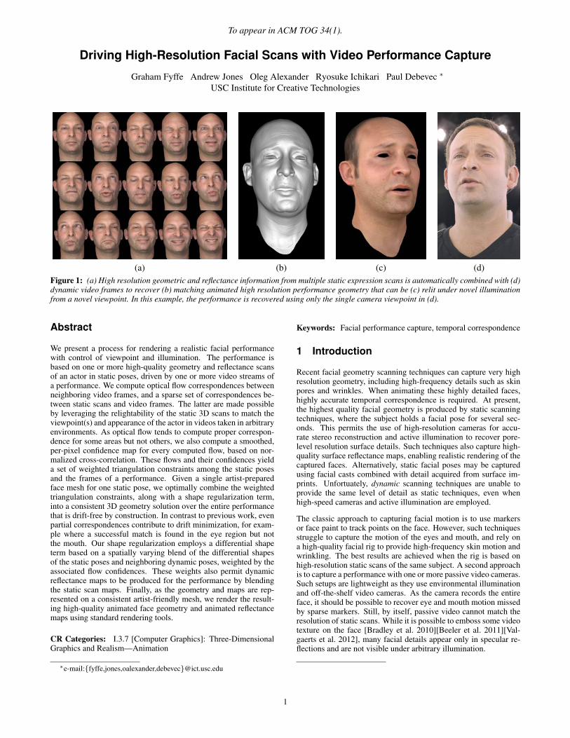
To appear in ACM TOG 34(1).

Driving High-Resolution Facial Scans with Video Performance Capture

Graham Fyffe Andrew Jones Oleg Alexander Ryosuke Ichikari Paul Debevec ∗

USC Institute for Creative Technologies

(a) (b) (c) (d)Figure 1: (a) High resolution geometric and reflectance information from multiple static expression scans is automatically combined with (d)dynamic video frames to recover (b) matching animated high resolution performance geometry that can be (c) relit under novel illuminationfrom a novel viewpoint. In this example, the performance is recovered using only the single camera viewpoint in (d).

Abstract

We present a process for rendering a realistic facial performancewith control of viewpoint and illumination. The performance isbased on one or more high-quality geometry and reflectance scansof an actor in static poses, driven by one or more video streams ofa performance. We compute optical flow correspondences betweenneighboring video frames, and a sparse set of correspondences be-tween static scans and video frames. The latter are made possibleby leveraging the relightability of the static 3D scans to match theviewpoint(s) and appearance of the actor in videos taken in arbitraryenvironments. As optical flow tends to compute proper correspon-dence for some areas but not others, we also compute a smoothed,per-pixel confidence map for every computed flow, based on nor-malized cross-correlation. These flows and their confidences yielda set of weighted triangulation constraints among the static posesand the frames of a performance. Given a single artist-preparedface mesh for one static pose, we optimally combine the weightedtriangulation constraints, along with a shape regularization term,into a consistent 3D geometry solution over the entire performancethat is drift-free by construction. In contrast to previous work, evenpartial correspondences contribute to drift minimization, for exam-ple where a successful match is found in the eye region but notthe mouth. Our shape regularization employs a differential shapeterm based on a spatially varying blend of the differential shapesof the static poses and neighboring dynamic poses, weighted by theassociated flow confidences. These weights also permit dynamicreflectance maps to be produced for the performance by blendingthe static scan maps. Finally, as the geometry and maps are rep-resented on a consistent artist-friendly mesh, we render the result-ing high-quality animated face geometry and animated reflectancemaps using standard rendering tools.

CR Categories: I.3.7 [Computer Graphics]: Three-DimensionalGraphics and Realism—Animation

∗e-mail:{fyffe,jones,oalexander,debevec}@ict.usc.edu

Keywords: Facial performance capture, temporal correspondence

1 Introduction

Recent facial geometry scanning techniques can capture very highresolution geometry, including high-frequency details such as skinpores and wrinkles. When animating these highly detailed faces,highly accurate temporal correspondence is required. At present,the highest quality facial geometry is produced by static scanningtechniques, where the subject holds a facial pose for several sec-onds. This permits the use of high-resolution cameras for accu-rate stereo reconstruction and active illumination to recover pore-level resolution surface details. Such techniques also capture high-quality surface reflectance maps, enabling realistic rendering of thecaptured faces. Alternatively, static facial poses may be capturedusing facial casts combined with detail acquired from surface im-prints. Unfortuately, dynamic scanning techniques are unable toprovide the same level of detail as static techniques, even whenhigh-speed cameras and active illumination are employed.

The classic approach to capturing facial motion is to use markersor face paint to track points on the face. However, such techniquesstruggle to capture the motion of the eyes and mouth, and rely ona high-quality facial rig to provide high-frequency skin motion andwrinkling. The best results are achieved when the rig is based onhigh-resolution static scans of the same subject. A second approachis to capture a performance with one or more passive video cameras.Such setups are lightweight as they use environmental illuminationand off-the-shelf video cameras. As the camera records the entireface, it should be possible to recover eye and mouth motion missedby sparse markers. Still, by itself, passive video cannot match theresolution of static scans. While it is possible to emboss some videotexture on the face [Bradley et al. 2010][Beeler et al. 2011][Val-gaerts et al. 2012], many facial details appear only in specular re-flections and are not visible under arbitrary illumination.

1

To appear in ACM TOG 34(1).

We present a technique for creating realistic facial animation froma set of high-resolution scans of an actor’s face, driven by passivevideo of the actor from one or more viewpoints. The videos can beshot under existing environmental illumination using off-the-shelfHD video cameras. The static scans can come from a variety ofsources including facial casts, passive stereo, or active illuminationtechniques. High-resolution detail and relightable reflectance prop-erties in the static scans can be transferred to the performance usinggenerated per-pixel weight maps. We operate our algorithm on aperformance flow graph that represents dense correspondences be-tween dynamic frames and multiple static scans, leveraging GPU-based optical flow to efficiently construct the graph. Besides a sin-gle artist remesh of a scan in neutral pose, our method requires norigging, no training of appearance models, no facial feature detec-tion, and no manual annotation of any kind. As a byproduct of ourmethod we also obtain a non-rigid registration between the artistmesh and each static scan. Our principal contributions are:

• An efficient scheme for selecting a sparse subset of imagepairs for optical flow computation for drift-free tracking.

• A fully coupled 3D tracking method with differential shaperegularization using multiple locally weighted target shapes.

• A message-passing-based optimization scheme leveraginglazy evaluation of energy terms enabling fully-coupled opti-mization over an entire performance.

2 Related Work

As many systems have been built for capturing facial geometry andreflectance, we will restrict our discussion to those that establishsome form of dense temporal correspondence over a performance.

Many existing algorithms compute temporal correspondence for asequence of temporally inconsistent geometries generated by e.g.structured light scanners or stereo algorithms. These algorithms op-erate using only geometric constraints [Popa et al. 2010] or by de-forming template geometry to match each geometric frame [Zhanget al. 2004]. The disadvantage of this approach is that the per-frame geometry often contains missing regions or erroneous ge-ometry which must be filled or filtered out, and any details that aremissed in the initial geometry solution are non-recoverable.

Other methods operate on video footage of facial performances.Methods employing frame-to-frame motion analysis are subjectto the accumulation of error or “drift” in the tracked geometry,prompting many authors to seek remedies for this issue. We there-fore limit our discussion to methods that make some effort to ad-dress drift. Li et al. [1993] compute animated facial blendshapeweights and rigid motion parameters to match the texture of eachvideo frame to a reference frame, within a local minimum deter-mined by a motion prediction step. Drift is avoided whenever asolid match can be made back to the reference frame. [DeCarloand Metaxas 1996] solves for facial rig control parameters to agreewith sparse monocular optical flow constraints, applying forces topull model edges towards image edges in order to combat drift.[Guenter et al. 1998] tracks motion capture dots in multiple views todeform a neutral facial scan, increasing the realism of the renderedperformance by projecting video of the face (with the dots digitallyremoved) onto the deforming geometry. The ”Universal Capture”system described in [Borshukov et al. 2003] dispenses with the dotsand uses dense multi-view optical flow to propagate vertices froman initial neutral expression. User intervention is required to cor-rect drift when it occurs. [Hawkins et al. 2004] uses performancetracking to automatically blend between multiple high-resolutionfacial scans per facial region, achieving realistic multi-scale facialdeformation without the need for reprojecting per-frame video, but

uses dots to avoid drift. Bradley et al. [2010] track motion us-ing dense multi-view optical flow, with a final registration step be-tween the neutral mesh and every subsequent frame to reduce drift.Beeler et al. [2011] explicitly identify anchor frames that are similarto a manually chosen reference pose using a simple image differ-ence metric, and track the performance bidirectionally between an-chor frames. Non-sequential surface tracking [Klaudiny and Hilton2012] finds a minimum-cost spanning tree over the frames in a per-formance based on sparse feature positions, tracking facial geome-try across edges in the tree with an additional temporal fusion step.Valgaerts et al. [2012] apply scene flow to track binocular passivevideo with a regularization term to reduce drift.

One drawback to all such optical flow tracking algorithms is that theface is tracked from one pose to another as a whole, and success ofthe tracking depends on accurate optical flow between images of theentire face. Clearly, the human face is capable of repeating differ-ent poses over different parts of the face asynchronously, which theholistic approaches fail to model. For example, if the subject is talk-ing with eyebrows raised and later with eyebrows lowered, a holis-tic approach will fail to exploit similarities in mouth poses wheneyebrow poses differ. In contrast, our approach constructs a graphconsidering similarities over multiple regions of the face across theperformance frames and a set of static facial scans, removing theneed for sparse feature tracking or anchor frame selection.

Blend-shape based animation rigs are also used to reconstruct dy-namic poses based on multiple face scans. The company ImageMetrics (now Faceware) has developed commercial software fordriving a blend-shape rig with passive video based on active appear-ance models [Cootes et al. 1998]. Weise et al. [2011] automaticallyconstruct a personalized blend shape rig and drive it with Kinectdepth data using a combination of as-rigid-as-possible constraintsand optical flow. In both cases, the quality of the resulting trackedperformance is directly related to the quality of the rig. Eachtracked frame is a linear combination of the input blend-shapes,so any performance details that lie outside the domain spanned bythe rig will not be reconstructed. Huang et al. [2011] automati-cally choose a minimal set of blend shapes to scan based on previ-ously captured performance with motion capture markers. Recre-ating missing detail requires artistic effort to add corrective shapesand cleanup animation curves [Alexander et al. 2009]. There hasbeen some research into other non-traditional rigs incorporatingscan data. Ma et al. [2008] fit a polynomial displacement map todynamic scan training data and generate detailed geometry fromsparse motion capture markers. Bickel et al. [2008] locally inter-polate a set of static poses using radial basis functions driven bymotion capture markers. Our method combines the shape regu-larization advantages of blendshapes with the flexibility of opticalflow based tracking. Our optimization algorithm leverages 3D in-formation from static scans without constraining the result to lieonly within the linear combinations of the scans. At the same time,we obtain per-pixel blend weights that can be used to produce per-frame reflectance maps.

3 Data Capture and Preparation

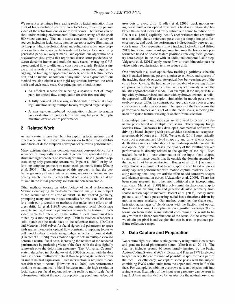
We capture high-resolution static geometry using multi-view stereoand gradient-based photometric stereo [Ghosh et al. 2011]. Thescan set includes around 30 poses largely inspired by the FacialAction Coding System (FACS) [Ekman and Friesen 1978], selectedto span nearly the entire range of possible shapes for each part ofthe face. For efficiency, we capture some poses with the subjectcombining FACS action units from the upper and lower half of theface. For example, combining eyebrows raise and cheeks puff intoa single scan. Examples of the input scan geometry can be seen inFig. 2. A base mesh is defined by an artist for the neutral pose scan.

2

To appear in ACM TOG 34(1).

The artist mesh has an efficient layout with edge loops followingthe wrinkles of the face. The non-neutral poses are represented asraw scan geometry, requiring no artistic topology or remeshing.

We capture dynamic performances using up to six Canon 1DXDSLR cameras under constant illumination. In the simplest case,we use the same cameras that were used for the static scans andswitch to 1920×1080 30p movie mode. We compute a sub-frame-accurate synchronization offset between cameras using a correla-tion analysis of the audio tracks. This could be omitted if cam-eras with hardware synchronization are employed. Following eachperformance, we capture a video frame of a calibration target tocalibrate camera intrinsics and extrinsics. We relight (and whennecessary, repose) the static scan data to resemble the illuminationconditions observed in the performance video. In the simplest case,the illumination field resembles one of the photographs taken dur-ing the static scan process and no relighting is required.

Figure 2: Sample static scans (showing geometry only).

4 The Performance Flow Graph

Optical-flow-based tracking algorithms such as [Bradley et al.2010][Beeler et al. 2011][Klaudiny and Hilton 2012] relate framesof a performance to each other based on optical flow correspon-dences over a set of image pairs selected from the performance.These methods differ in part by the choice of the image pairs to beemployed. We generalize this class of algorithms using a structurewe call the performance flow graph, which is a complete graph withedges representing dense 2D correspondences between all pairs ofimages, with each edge having a weight, or confidence, of the as-sociated estimated correspondence field. The graphs used in previ-ous works, including anchor frames [Beeler et al. 2011] and non-sequential alignment with temporal fusion [Klaudiny and Hilton2012], can be represented as a performance flow graph having unitweight for the edges employed by the respective methods, and zeroweight for the unused edges. We further generalize the performanceflow graph to include a dense confidence field associated with eachcorrespondence field, allowing the confidence to vary spatially overthe image. This enables our technique to exploit relationships be-tween images where only a partial correspondence was able to becomputed (for example, a pair of images where the mouth is similarbut the eyes are very different). Thus our technique can be viewedas an extension of anchor frames or minimum spanning trees tominimize drift independently over different regions of the face.

A performance capture system that considers correspondences be-tween all possible image pairs naturally minimizes drift. However,this would require an exorbitant number of graph edges, so we in-stead construct a graph with a reduced set of edges that approxi-mates the complete graph, in the sense that the correspondences arerepresentative of the full set with respect to confidence across theregions of the face. Our criterion for selecting the edges to includein the performance flow graph is that any two images having a high

DYNAMIC SEQUENCE

STATIC SCANS

Figure 3: performance flow graph showing optical flow correspon-dences between static and dynamic images. Red lines represent op-tical flow between neighboring frames within a performance. Blue,green, and orange lines represent optical flow between dynamic andstatic images. Based on initial low-resolution optical flow, we con-struct a sparse graph requiring only a small subset of high resolu-tion flows to be computed between static scans and dynamic frames.

confidence correspondence between them in the complete graph ofpossible correspondences ought to have a path between them (aconcatenation of one or more correspondences) in the constructedgraph with nearly as high confidence (including the reduction inconfidence from concatenation). We claim that correspondencesbetween temporally neighboring dynamic frames are typically ofhigh quality, and no concatenation of alternative correspondencescan be as confident, therefore we always include a graph edge be-tween each temporally neighboring pair of dynamic frames. Cor-respondences between frames with larger temporal gaps are well-approximated by concatenating neighbors, but decreasingly so overlarger temporal gaps (due to drift). We further claim that wheneverenough drift accumulates to warrant including a graph edge overthe larger temporal gap, there exists a path with nearly as good con-fidence that passes through one of the predetermined static scans(possibly a different static scan for each region of the face). We jus-tify this claim by noting the 30 static poses based on FACS oughtto span the space of performances well enough that any region ofany dynamic frame can be corresponded to some region in somestatic scan with good confidence. Therefore we do not includeany edges between non-neighboring dynamic frames, and insteadconsider only edges between a static scan and a dynamic frame ascandidates for inclusion (visualized in Fig. 3). Finally, as the driftaccumulated from the concatenation described above warrants ad-ditional edges only sparsely over time, we devise a coarse-to-finegraph construction strategy using only a sparse subset of static-to-dynamic graph edges. We detail this strategy in Section 4.1.

4.1 Constructing the Performance Flow Graph

The images used in our system consist of one or more dynamicsequences of frames captured from one or more viewpoints, androughly similar views of a set of high-resolution static scans. Thenodes in our graph represent static poses (associated with staticscans) and dynamic poses (associated with dynamic frames fromone or more sequences). We construct the performance flow graphby computing a large set of static-to-dynamic optical flow corre-spondences at a reduced resolution for only a single viewpoint, and

3

To appear in ACM TOG 34(1).

then omit redundant correspondences using a novel voting algo-rithm to select a sparse set of correspondences that is representativeof the original set. We then compute high-quality optical flow cor-respondences at full resolution for the sparse set, and include allviewpoints. The initial set of correspondences consists of quarter-resolution optical flows from each static scan to every nth dynamicframe. For most static scans we use every 5th dynamic frame, whilefor the eyes-closed scan we use every dynamic frame in order tocatch rapid eye blinks. We then compute normalized cross corre-lation fields between the warped dynamic frames and each originalstatic scan to evaluate the confidence of the correspondences. Thesecorrespondences may be computed in parallel over multiple com-puters, as there is no sequential dependency between them. We findthat at quarter resolution, flow-based cross correlation correctly as-signs low confidence to incorrectly matched facial features, for ex-ample when flowing disparate open and closed mouth shapes. Toreduce noise and create a semantically meaningful metric, we av-erage the resulting confidence over twelve facial regions (see Fig.4). These facial regions are defined once on the neutral pose, andare warped to all other static poses using rough static-to-static opti-cal flow. Precise registration of regions is not required, as they areonly used in selecting the structure of the performance graph. Inthe subsequent tracking phase, per-pixel confidence is used.

(a) (b) (c) (d)

(e) (f)

Figure 4: We compute an initial low-resolution optical flow be-tween a dynamic image (a) and static image (b). We then com-pute normalized cross correlation between the static image (b) andthe warped dynamic image (c) to produce the per-pixel confidenceshown in (d). We average these values for 12 regions (e) to obtaina per-region confidence value (f). This example shows correlationbetween the neutral scan and a dynamic frame with the eyebrowsraised and the mouth slightly open. The forehead and mouth re-gions are assigned appropriately lower confidences.

Ideally we want the performance flow graph to be sparse. Besidestemporally adjacent poses, dynamic poses should only connect tosimilar static poses and edges should be evenly distributed over timeto avoid accumulation of drift. We propose an iterative greedy vot-ing algorithm based on the per-region confidence measure to iden-tify good edges. The confidence of correspondence between the dy-namic frames and any region of any static facial scan can be viewedas a curve over time (depicted in Fig. 5). In each iteration we iden-tify the maximum confidence value over all regions, all scans, andall frames. We add an edge between the identified dynamic pose

0 50 100 150 200 250 300 350 4000

0.2

0.4

0.6

0.8

frame number

conf

iden

ce

ForeheadMouth

10 70 130 180 270 320

Figure 5: A plot of the per-region confidence metric over time.Higher numbers indicate greater correlation between the dynamicframes and a particular static scan. The cyan curve represents thecenter forehead region of a brows-raised static scan which is ac-tive throughout the later sequence. The green curve represents themouth region for an extreme mouth-open scan which is active onlywhen the mouth opens to its fullest extent. The dashed lines indicatethe timing of the sampled frames shown on the bottom row.

and static pose to the graph. We then adjust the recorded confidenceof the identified region by subtracting a hat function scaled by themaximum confidence and centered around the maximum frame, in-dicating that the selected edge has been accounted for, and temporalneighbors partly so. All other regions are adjusted by subtractingsimilar hat functions, scaled by the (non-maximal) per-region con-fidence of the identified flow. This suppresses any other regions thatare satisfied by the flow. The slope of the hat function represents aloss of confidence as this flow is combined with adjacent dynamic-to-dynamic flows. We then iterate and choose the new highest con-fidence value, until all confidence values fall below a threshold. Thetwo parameters (the slope of the hat function and the final thresh-old value) provide intuitive control over the total number of graphedges. We found a reasonable hat function falloff to be a 4% re-duction for every temporal flow and a threshold value that is 20%of the initial maximum confidence. After constructing the graph,a typical 10-20 second performance flow graph will contain 100-200 edges between dynamic and static poses. Again, as the changebetween sequential frames is small, we preserve all edges betweenneighboring dynamic poses.

After selecting the graph edges, final HD resolution optical flowsare computed for all active cameras and for all retained graph edges.We directly load video frames using nVidia’s h264 GPU decoderand feed them to the FlowLib implementation of GPU-optical flow[Werlberger 2012]. Running on a Nvidia GTX 680, computationof quarter resolution flows for graph construction take less than onesecond per flow. Full-resolution HD flows for dynamic-to-dynamicimages take 8 seconds per flow, and full-resolution flows betweenstatic and dynamic images take around 23 seconds per flow due toa larger search window. More sophisticated correspondence esti-mation schemes could be employed within our framework, but ourintention is that the framework be agnostic to this choice and ro-bust to imperfections in the pairwise correspondences. After com-puting optical flows and confidences, we synchronize all the flowsequences to a primary camera by warping each flow frame for-ward or backward in time based on the sub-frame synchronizationoffsets between cameras.

We claim that an approximate performance flow graph constructedin this manner is more representative of the complete set of possible

4

To appear in ACM TOG 34(1).

correspondences than previous methods that take an all-or-nothingapproach to pair selection, while still employing a number of opti-cal flow computations on the same order as previous methods (i.e.temporal neighbors plus additional sparse image pairs).

5 Fully Coupled Performance Tracking

The performance flow graph is representative of all the constraintswe could glean from 2D correspondence analysis of the input im-ages, and now we aim to put those constraints to work. We formu-late an energy function in terms of the 3D vertex positions of theartist mesh as it deforms to fit all of the dynamic and static poses inthe performance flow graph in a common head coordinate system,as well as the associated head-to-world rigid transforms. We collectthe free variables into a vector θ = (xp

i ,Rp, tp|p ∈ D∪S, i ∈ V),where xp

i represents the 3D vertex position of vertex i at pose pin the common head coordinate system, Rp and tp represent therotation matrix and translation vector that rigidly transform pose pfrom the common head coordinate system to world coordinates, Dis the set of dynamic poses, S is the set of static poses, and V is theset of mesh vertices. The energy function is then:

E(θ) =∑

(p,q)∈F

(Epqcorr + Eqp

corr) + λ∑

p∈D∪S

|Fp|Epshape

+ ζ∑p∈S

|Fp|Epwrap + γ|Fg|Eground, (1)

where F is the set of performance flow graph edges, Fp is the sub-set of edges connecting to pose p, and g is the ground (neutral)static pose. This function includes:

• dense correspondence constraints Epqcorr associated with the

edges of the performance flow graph,

• shape regularization terms Epshape relating the differential

shape of dynamic and static poses to their graph neighbors,

• “shrink wrap” terms Epwrap to conform the static poses to the

surface of the static scan geometries,

• a final grounding term Eground to prefer the vertex positionsin a neutral pose to be close to the artist mesh vertex positions.

We detail these terms in sections 5.2 - 5.5. Note we do not em-ploy a stereo matching term, allowing our technique to be robust tosmall synchronization errors between cameras. As the number ofposes and correspondences may vary from one dataset to another,the summations in (1) contain balancing factors (to the immediateright of each Σ) in order to have comparable total magnitude (pro-portional to |F|). The terms are weighted by tunable term weightsλ, ζ and γ, which in all examples we set equal to 1.

5.1 Minimization by Lazy DDMS-TRWS

In contrast to previous work, we consider the three-dimensionalcoupling between all terms in our formulation, over all dynamic andstatic poses simultaneously, thereby obtaining a robust estimate thatgracefully fills in missing or unreliable information. This presentstwo major challenges. First, the partial matches and loops in theperformance flow graph preclude the use of straightforward meshpropagation schemes used in previous works. Such propagationwould produce only partial solutions for many poses. Second (as aresult of the first) we lack a complete initial estimate for traditionaloptimization schemes such as Levenberg-Marquadt.

To address these challenges, we employ an iterative scheme thatadmits partial intermediate solutions, with pseudocode in Algo-rithm 1. As some of the terms in (1) are data-dependent, we

adapt the outer loop of Data Driven Mean-Shift Belief Propagation(DDMSBP) [Park et al. 2010], which models the objective functionin each iteration as an increasingly-tight Gaussian (or quadratic)approximation of the true function. Within each DDMS loop, weuse Gaussian Tree-Reweighted Sequential message passing (TRW-S) [Kolmogorov 2006], adapted to allow the terms in the model tobe constructed lazily as the solution progresses over the variables.Hence we call our scheme Lazy DDMS-TRWS. We define the or-dering of the variables to be pose-major (i.e. visiting all the verticesof one pose, then all the vertices of the next pose, etc.), with staticposes followed by dynamic poses in temporal order. We decom-pose the Gaussian belief as a product of 3D Gaussians over verticesand poses, which admits a pairwise decomposition of (1) as a sumof quadratics. We denote the current belief of a vertex i for pose pas xp

i with covariance Σpi (stored as inverse covariance for conve-

nience), omitting the i subscript to refer to all vertices collectively.We detail the modeling of the energy terms in sections 5.2 - 5.5,defining yp

i = Rpxpi + tp as shorthand for world space vertex

position estimates. We iterate the DDMS loop 6 times, and iterateTRW-S until 95% of the vertices converge to within 0.01mm.

Algorithm 1 Lazy DDMS-TRWS for (1)

∀p,i : (Σpi )−1← 0.

for DDMS outer iterations do// Reset the model:∀p,q : Epq

corr,Epshape,E

pwrap← undefined (effectively 0).

for TRW-S inner iterations do// Major TRW-S loop over poses:for each p ∈ D ∪ S in order of increasing o(p) do

// Update model where possible:for each q|(p, q) ∈ F do

if (Σp)−1 6= 0 and Epqcorr undefined then

Epqcorr← model fit using (2) in section 5.2.

if (Σq)−1 6= 0 and Eqpcorr undefined then

Eqpcorr← model fit using (2) in section 5.2.

if (Σp)−1 6= 0 and Epwrap undefined then

Epwrap← model fit using (8) in section 5.4.

if ∃(p,q)∈F |(Σq)−1 6= 0 and Epshape undefined then

Epshape← model fit using (5) in section 5.3.

// Minor TRW-S loop over vertices:Pass messages based on (1) to update xp, (Σp)−1.Update Rp, tp as in section 5.6.

// Reverse TRW-S ordering:o(s)← ‖D ∪ S‖+ 1− o(s).

5.2 Modeling the Correspondence Term

The correspondence term in (1) penalizes disagreement betweenoptical flow vectors and projected vertex locations. Suppose wehave a 2D optical flow correspondence field between poses p and qin (roughly) the same view c. We may establish a 3D relationshipbetween xp

i and xqi implied by the 2D correspondence field, which

we model as a quadratic penalty function:

Epqcorr = 1

|C|

∑∑c∈Ci∈V

(xqi − xp

i − f cpqi

)TFcpqi

(xqi − xp

i − f cpqi

), (2)

where C is the set of camera viewpoints, and f cpqi,Fc

pqi

are respec-tively the mean and precision matrix of the penalty, which we es-timate from the current estimated positions as follows. We firstproject yp

i into the image plane of view c of pose p. We then warpthe 2D image position from view c of pose p to view c of pose q

5

To appear in ACM TOG 34(1).

using the correspondence field. The warped 2D position defines aworld-space view ray that the same vertex i ought to lie on in poseq. We transform this ray back into common head coordinates (via−tq , RT

q ) and penalize the squared distance from xqi to this ray.

Letting rcpqi

represent the direction of this ray, this yields:

f cpqi

= (I− rcpqi

rcpqi

T)(RTq (cc

q − tq)− xpi ), (3)

where ccq is the nodal point of view c of pose q, and rcpq

i= RT

qdcpqi

with dcpqi

the world-space direction of the ray in view c of pose

q through the 2D image plane point fcpq[Pc

p (ypi )] (where square

brackets represent bilinearly interpolated sampling of a field or im-age), fc

pq the optical flow field transforming an image-space pointfrom view c of pose p to the corresponding point in view c of poseq, and Pc

p(x) the projection of a point x into the image plane ofview c of pose p (which may differ somewhat from pose to pose).If we were to use the squared-distance-to-ray penalty directly, Fc

pqi

would be I − rcpqi

rcpqi

T, which is singular. To prevent the problemfrom being ill-conditioned and also to enable the use of monocularperformance data, we add a small regularization term to producea non-singular penalty, and weight the penalty by the confidenceof the optical flow estimate. We also assume the optical flow fieldis locally smooth, so a large covariance Σp

i inversely influencesthe precision of the model, whereas a small covariance Σp

i doesnot, and weight the model accordingly. Intuitively, this weightingcauses information to propagate from the ground term outward viathe correspondences in early iterations, and blends correspondencesfrom all sources in later iterations. All together, this yields:

Fcpqi

= min(1, det(Σpi )−

13 )vcp

iτ cpq[Pc

p(ypi )](I−rcpq

ircpqi

T+εI), (4)

where vcpi

is a soft visibility factor (obtained by blurring a binaryvertex visibility map and modulated by the cosine of the angle be-tween surface normal and view direction), τ cpq is the confidencefield associated with the correspondence field fc

pq , and ε is a smallregularization constant. We use det(Σ)−1/3 as a scalar form ofprecision for 3D Gaussians.

5.3 Modeling the Differential Shape Term

The shape term in (1) constrains the differential shape of each poseto a spatially varying convex combination of the differential shapesof the neighboring poses in the performance flow graph:

Epshape =

∑(i,j)∈E

∥∥xpj − xp

i − lpij∥∥2, (5)

lpij =ε(gj − gi) +

∑q|(p,q)∈F wpq

ij (xqj − xq

i )

ε+∑

q|(p,q)∈F wpqij

, (6)

wpqij =

wpqi w

pqj

wpqi + wpq

j

, (7)

where E is the set of edges in the geometry mesh, wpqi =

det( 1|C|∑

c∈C Fcpqi

+Fcqpi

)1/3 (which is intuitively the strength ofthe relationship between poses p and q due to the correspondenceterm), g denotes the artist mesh vertex positions, and ε is a smallregularization constant. The weights wpq

i additionally enable triv-ial synthesis of high-resolution reflectance maps for each dynamicframe of the performance by blending the static pose data.

5.4 Modeling the Shrink Wrap Term

The shrink wrap term in (1) penalizes the distance between staticpose vertices and the raw scan geometry of the same pose. We

model this as a regularized distance-to-plane penalty:

Epwrap =

∑i∈V

(xpi − dp

i )Tgpi (np

i npiT+ εI)(xp

i − dpi ), (8)

where (npi ,d

pi ) are the normal and centroid of a plane fitted to the

surface of the static scan for pose p close to the current estimatexpi in common head coordinates, and gp

i is the confidence of theplanar fit. We obtain the planar fit inexpensively by projecting yp

i

into each camera view, and sampling the raw scan surface via aset of precomputed rasterized views of the scan. (Alternatively, a3D search could be employed to obtain the samples.) Each surfacesample (excluding samples that are occluded or outside the raster-ized scan) provides a plane equation based on the scan geometryand surface normal. We let np

i and dpi be the weighted average

values of the plane equations over all surface samples:

npi =

∑c∈C

ωcpiRT

p ncp[Pc

p(ypi )] (normalized), (9)

dpi =

(∑c∈C

ωcpi

)−1∑c∈C

ωcpiRT

p(dcp[Pc

p(ypi )]− tp), (10)

gpi = min(1, det(Σp

i )−13 )∑c∈C

ωcpi, (11)

where (ncp, d

cp) are the world-space surface normal and position

images of the rasterized scans, and ωcpi

= 0 if the vertex is occludedin view c or lands outside of the rasterized scan, otherwise ωc

pi

=

vcpi

exp(−‖dcp[Pc

p(ypi )]− yp

i ‖2).

5.5 Modeling the Ground Term

The ground term in (1) penalizes the distance between vertex po-sitions in the ground (neutral) pose and the artist mesh geometry:

Eground =∑i∈V

∥∥∥xgi −RT

ggi

∥∥∥2, (12)

where gi is the position of the vertex in the artist mesh. This termis simpler than the shrink-wrap term since the pose vertices are inone-to-one correspondence with the artist mesh vertices.

5.6 Updating the Rigid Transforms

We initialize our optimization scheme with all (Σpi )−1 = 0 (and

hence all xpi moot), fully relying on the lazy DDMS-TRWS scheme

to propagate progressively tighter estimates of the vertex positionsxpi throughout the solution. Unfortunately, in our formulation the

rigid transforms (Rp, tp) enjoy no such treatment as they alwaysoccur together with xp

i and would produce non-quadratic termsif they were included in the message passing domain. There-fore we must initialize the rigid transforms to some rough ini-tial guess, and update them after each iteration. The neutral poseis an exception, where the transform is specified by the user (byrigidly posing the artist mesh to their whim) and hence not up-dated. In all our examples, the initial guess for all poses is sim-ply the same as the user-specified rigid transform of the neutralpose. We update (Rp, tp) using a simple scheme that aligns theneutral artist mesh to the current result. Using singular valuedecomposition, we compute the closest rigid transform minimiz-ing

∑i∈V ri

∥∥Rpgi + tp − Rpxpi − tp

∥∥2, where ri is a rigidityweight value (high weight around the eye sockets and temples, lowweight elsewhere), gi denotes the artist mesh vertex positions, and(Rp, tp) is the previous transform estimate.

6

To appear in ACM TOG 34(1).

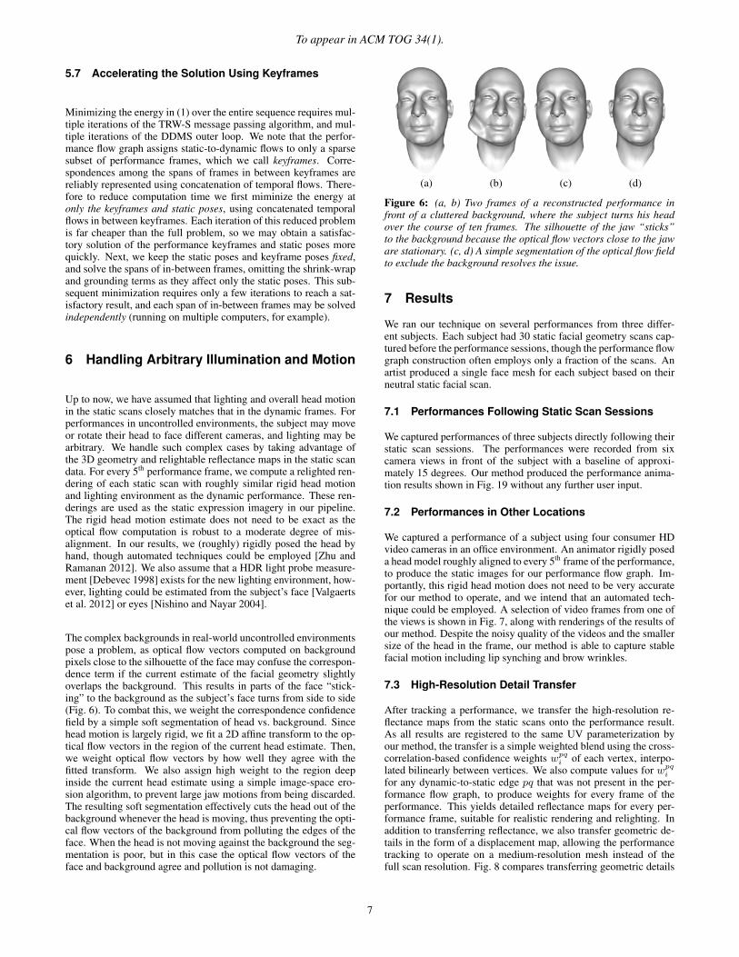
5.7 Accelerating the Solution Using Keyframes

Minimizing the energy in (1) over the entire sequence requires mul-tiple iterations of the TRW-S message passing algorithm, and mul-tiple iterations of the DDMS outer loop. We note that the perfor-mance flow graph assigns static-to-dynamic flows to only a sparsesubset of performance frames, which we call keyframes. Corre-spondences among the spans of frames in between keyframes arereliably represented using concatenation of temporal flows. There-fore to reduce computation time we first miminize the energy atonly the keyframes and static poses, using concatenated temporalflows in between keyframes. Each iteration of this reduced problemis far cheaper than the full problem, so we may obtain a satisfac-tory solution of the performance keyframes and static poses morequickly. Next, we keep the static poses and keyframe poses fixed,and solve the spans of in-between frames, omitting the shrink-wrapand grounding terms as they affect only the static poses. This sub-sequent minimization requires only a few iterations to reach a sat-isfactory result, and each span of in-between frames may be solvedindependently (running on multiple computers, for example).

6 Handling Arbitrary Illumination and Motion

Up to now, we have assumed that lighting and overall head motionin the static scans closely matches that in the dynamic frames. Forperformances in uncontrolled environments, the subject may moveor rotate their head to face different cameras, and lighting may bearbitrary. We handle such complex cases by taking advantage ofthe 3D geometry and relightable reflectance maps in the static scandata. For every 5th performance frame, we compute a relighted ren-dering of each static scan with roughly similar rigid head motionand lighting environment as the dynamic performance. These ren-derings are used as the static expression imagery in our pipeline.The rigid head motion estimate does not need to be exact as theoptical flow computation is robust to a moderate degree of mis-alignment. In our results, we (roughly) rigidly posed the head byhand, though automated techniques could be employed [Zhu andRamanan 2012]. We also assume that a HDR light probe measure-ment [Debevec 1998] exists for the new lighting environment, how-ever, lighting could be estimated from the subject’s face [Valgaertset al. 2012] or eyes [Nishino and Nayar 2004].

The complex backgrounds in real-world uncontrolled environmentspose a problem, as optical flow vectors computed on backgroundpixels close to the silhouette of the face may confuse the correspon-dence term if the current estimate of the facial geometry slightlyoverlaps the background. This results in parts of the face “stick-ing” to the background as the subject’s face turns from side to side(Fig. 6). To combat this, we weight the correspondence confidencefield by a simple soft segmentation of head vs. background. Sincehead motion is largely rigid, we fit a 2D affine transform to the op-tical flow vectors in the region of the current head estimate. Then,we weight optical flow vectors by how well they agree with thefitted transform. We also assign high weight to the region deepinside the current head estimate using a simple image-space ero-sion algorithm, to prevent large jaw motions from being discarded.The resulting soft segmentation effectively cuts the head out of thebackground whenever the head is moving, thus preventing the opti-cal flow vectors of the background from polluting the edges of theface. When the head is not moving against the background the seg-mentation is poor, but in this case the optical flow vectors of theface and background agree and pollution is not damaging.

(a) (b) (c) (d)

Figure 6: (a, b) Two frames of a reconstructed performance infront of a cluttered background, where the subject turns his headover the course of ten frames. The silhouette of the jaw “sticks”to the background because the optical flow vectors close to the jaware stationary. (c, d) A simple segmentation of the optical flow fieldto exclude the background resolves the issue.

7 Results

We ran our technique on several performances from three differ-ent subjects. Each subject had 30 static facial geometry scans cap-tured before the performance sessions, though the performance flowgraph construction often employs only a fraction of the scans. Anartist produced a single face mesh for each subject based on theirneutral static facial scan.

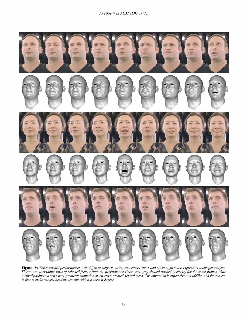
7.1 Performances Following Static Scan Sessions

We captured performances of three subjects directly following theirstatic scan sessions. The performances were recorded from sixcamera views in front of the subject with a baseline of approxi-mately 15 degrees. Our method produced the performance anima-tion results shown in Fig. 19 without any further user input.

7.2 Performances in Other Locations

We captured a performance of a subject using four consumer HDvideo cameras in an office environment. An animator rigidly poseda head model roughly aligned to every 5th frame of the performance,to produce the static images for our performance flow graph. Im-portantly, this rigid head motion does not need to be very accuratefor our method to operate, and we intend that an automated tech-nique could be employed. A selection of video frames from one ofthe views is shown in Fig. 7, along with renderings of the results ofour method. Despite the noisy quality of the videos and the smallersize of the head in the frame, our method is able to capture stablefacial motion including lip synching and brow wrinkles.

7.3 High-Resolution Detail Transfer

After tracking a performance, we transfer the high-resolution re-flectance maps from the static scans onto the performance result.As all results are registered to the same UV parameterization byour method, the transfer is a simple weighted blend using the cross-correlation-based confidence weights wpq

i of each vertex, interpo-lated bilinearly between vertices. We also compute values for wpq

i

for any dynamic-to-static edge pq that was not present in the per-formance flow graph, to produce weights for every frame of theperformance. This yields detailed reflectance maps for every per-formance frame, suitable for realistic rendering and relighting. Inaddition to transferring reflectance, we also transfer geometric de-tails in the form of a displacement map, allowing the performancetracking to operate on a medium-resolution mesh instead of thefull scan resolution. Fig. 8 compares transferring geometric details

7

To appear in ACM TOG 34(1).

Figure 7: A performance captured in an office environment with uncontrolled illumination, using four HD consumer video cameras andseven static expression scans. Top row: a selection of frames from one of the camera views. Middle row: geometry tracked using theproposed method, with reflectance maps automatically assembled from static scan data, shaded using a high-dynamic-range light probe. Thereflectance of the top and back of the head were supplemented with artist-generated static maps. The eyes and inner mouth are rendered asblack as our method does not track these features. Bottom row: gray-shaded geometry for the same frames, from a novel viewpoint. Ourmethod produces stable animation even with somewhat noisy video footage and significant head motion. Dynamic skin details such as browwrinkles are transferred from the static scans in a manner faithful to the video footage.

(a) (b) (c)

Figure 8: High-resolution details may be transferred to a medium-resolution tracked model to save computation time. (a) medium-resolution tracked geometry using six views. (b) medium-resolutiongeometry with details automatically transferred from the high-resolution static scans. (c) high-resolution tracked geometry. Thetransferred details in (b) capture most of the dynamic facial detailsseen in (c) at a reduced computational cost.

from the static scans onto a medium-resolution reconstruction to di-rectly tracking a high-resolution mesh. As the high-resolution solveis more expensive, we first perform the medium-resolution solveand use it to prime the DDMS-TRWS belief in the high-resolutionsolve, making convergence more rapid. In all other results, we showmedium-resolution tracking with detail transfer, as the results aresatisfactory and far cheaper to compute.

Figure 9: Results using only a single camera view, showing the lastfour frames from Fig. 7. Even under uncontrolled illumination andsignificant head motion, tracking is possible from a single view, atsomewhat reduced fidelity.

7.4 Monocular vs. Binocular vs. Multi-View

Our method operates on any number of camera views, producinga result from even a single view. Fig. 9 shows results from a sin-gle view for the same uncontrolled-illumination sequence as Fig.7. Fig. 10 shows the incremental improvement in facial detail fora controlled-illumination sequence using one, two, and six views.Our method is applicable to a wide variety of camera and lightingsetups, with graceful degradation as less information is available.

7.5 Influence of Each Energy Term

The core operation of our method is to propagate a known facialpose (the artist mesh) to a set of unknown poses (the dynamicframes and other static scans) via the ground term and correspon-dence terms in our energy formulation. The differential shape termand shrink wrap term serve to regularize the shape of the solution.We next explore the influence of these terms on the solution.

8

To appear in ACM TOG 34(1).

(a) (b) (c)

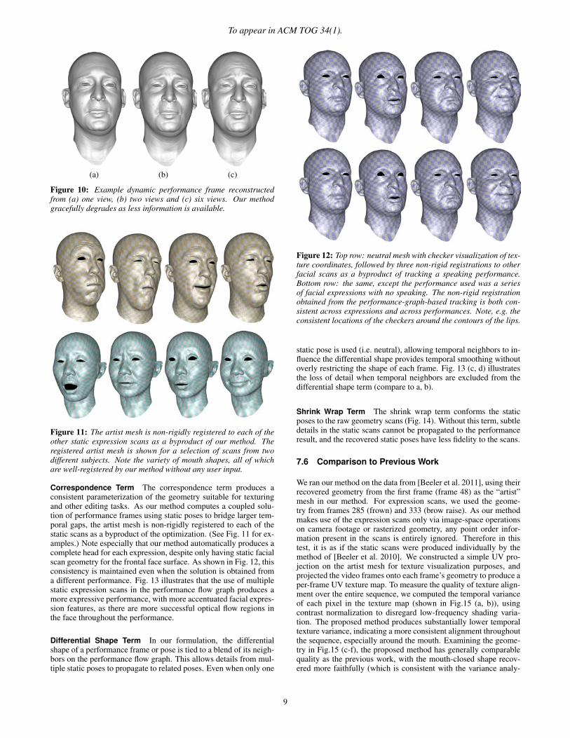
Figure 10: Example dynamic performance frame reconstructedfrom (a) one view, (b) two views and (c) six views. Our methodgracefully degrades as less information is available.

Figure 11: The artist mesh is non-rigidly registered to each of theother static expression scans as a byproduct of our method. Theregistered artist mesh is shown for a selection of scans from twodifferent subjects. Note the variety of mouth shapes, all of whichare well-registered by our method without any user input.

Correspondence Term The correspondence term produces aconsistent parameterization of the geometry suitable for texturingand other editing tasks. As our method computes a coupled solu-tion of performance frames using static poses to bridge larger tem-poral gaps, the artist mesh is non-rigidly registered to each of thestatic scans as a byproduct of the optimization. (See Fig. 11 for ex-amples.) Note especially that our method automatically produces acomplete head for each expression, despite only having static facialscan geometry for the frontal face surface. As shown in Fig. 12, thisconsistency is maintained even when the solution is obtained froma different performance. Fig. 13 illustrates that the use of multiplestatic expression scans in the performance flow graph produces amore expressive performance, with more accentuated facial expres-sion features, as there are more successful optical flow regions inthe face throughout the performance.

Differential Shape Term In our formulation, the differentialshape of a performance frame or pose is tied to a blend of its neigh-bors on the performance flow graph. This allows details from mul-tiple static poses to propagate to related poses. Even when only one

Figure 12: Top row: neutral mesh with checker visualization of tex-ture coordinates, followed by three non-rigid registrations to otherfacial scans as a byproduct of tracking a speaking performance.Bottom row: the same, except the performance used was a seriesof facial expressions with no speaking. The non-rigid registrationobtained from the performance-graph-based tracking is both con-sistent across expressions and across performances. Note, e.g. theconsistent locations of the checkers around the contours of the lips.

static pose is used (i.e. neutral), allowing temporal neighbors to in-fluence the differential shape provides temporal smoothing withoutoverly restricting the shape of each frame. Fig. 13 (c, d) illustratesthe loss of detail when temporal neighbors are excluded from thedifferential shape term (compare to a, b).

Shrink Wrap Term The shrink wrap term conforms the staticposes to the raw geometry scans (Fig. 14). Without this term, subtledetails in the static scans cannot be propagated to the performanceresult, and the recovered static poses have less fidelity to the scans.

7.6 Comparison to Previous Work

We ran our method on the data from [Beeler et al. 2011], using theirrecovered geometry from the first frame (frame 48) as the “artist”mesh in our method. For expression scans, we used the geome-try from frames 285 (frown) and 333 (brow raise). As our methodmakes use of the expression scans only via image-space operationson camera footage or rasterized geometry, any point order infor-mation present in the scans is entirely ignored. Therefore in thistest, it is as if the static scans were produced individually by themethod of [Beeler et al. 2010]. We constructed a simple UV pro-jection on the artist mesh for texture visualization purposes, andprojected the video frames onto each frame’s geometry to produce aper-frame UV texture map. To measure the quality of texture align-ment over the entire sequence, we computed the temporal varianceof each pixel in the texture map (shown in Fig.15 (a, b)), usingcontrast normalization to disregard low-frequency shading varia-tion. The proposed method produces substantially lower temporaltexture variance, indicating a more consistent alignment throughoutthe sequence, especially around the mouth. Examining the geome-try in Fig.15 (c-f), the proposed method has generally comparablequality as the previous work, with the mouth-closed shape recov-ered more faithfully (which is consistent with the variance analy-

9

To appear in ACM TOG 34(1).

(a) (b) (c) (d)

Figure 13: Using multiple static expressions in the performanceflow graph produces more detail than using just a neutral staticexpression. Multiple static expressions are included in the perfor-mance flow graph in (a, c), whereas only the neutral expression isincluded in (b, d). By including temporal neighbors and static scansin determining the differential shape, details from the various staticscans can be propagated throughout the performance. Differentialshape is determined by the static expression(s) and temporal neigh-bors in (a, b), whereas temporal neighbors are excluded from thedifferential shape term in (c, d). Note the progressive loss of detailin e.g. the brow region from (a) to (d).

sis). We also compared to [Klaudiny and Hilton 2012] in a similarmanner, using frame 0 as the artist mesh, and frames 25, 40, 70,110, 155, 190, 225, 255 and 280 as static expressions. Again, nopoint order information is used. Fig. 16 again shows an overalllower temporal texture variance from the proposed method.

7.7 Performance Timings

We report performance timings in Fig. 17 for various sequences,running on a 16-core 2.4 GHz Xeon E5620 workstation (some oper-ations are multithreaded across the cores). All tracked meshes have65 thousand vertices, except Fig. 8(c) and Fig. 15 which have onemillion vertices. We report each stage of the process: “Graph” forthe performance graph construction, “Flow” for the high-resolutionoptical flow calculations, “Key” for the performance tracking solveon key frames, and “Tween” for the performance tracking solvein between key frames. We mark stages that could be parallelizedover multiple machines with an asterisk (*). High-resolution solves(Fig. 8(c) and Fig. 15) take longer than medium-resolution solves.Sequences with uncontrolled illumination (Fig. 7 and Fig. 9) takelonger for the key frames to converge since the correspondence ty-ing the solution to the static scans has lower confidence.

7.8 Discussion

Our method produces a consistent geometry animation on an artist-created neutral mesh. The animation is expressive and lifelike, andthe subject is free to make natural head movements within a cer-tain degree. Fig. 18 shows renderings from such a facial perfor-mance rendered using advanced skin and eye shading techniquesas described in [Jimenez et al. 2012]. One notable shortcoming ofour performance flow graph construction algorithm is the neglectof eye blinks. This results in a poor representation of the blinksin the final animation. Our method requires one artist-generatedmesh per subject to obtain results that are immediately usable inproduction pipelines. Automatic generation of this mesh couldbe future work, or use existing techniques for non-rigid registra-tion. Omitting this step would still produce a result, but would re-quire additional cleanup around the edges as in e.g. [Beeler et al.2011][Klaudiny and Hilton 2012].

(a) (b) (c)

(d) (e) (f)

Figure 14: The shrink wrap term conforms the artist mesh to thestatic scan geometry, and also improves the transfer of expressivedetails to the dynamic performance. The registered artist mesh isshown for two static poses in (a) and (b), and a dynamic pose thatborrows brow detail from (a) and mouth detail from (b) is shown in(c). Without the shrink wrap term, the registration to the static posessuffers (d, e) and the detail transfer to the dynamic performance isless sucessful (f). Fine-scale details are still transferred via dis-placement maps, but medium-scale expressive details are lost.

8 Future Work

One of the advantages of our technique is that it relates a dynamicperformance back to facial shape scans using per-pixel weightmaps. It would be desirable to further factor our results to cre-ate multiple localized blend shapes which are more semanticallymeaningful and artist friendly. Also, our algorithm does not explic-itly track eye or mouth contours. Eye and mouth tracking couldbe further refined with additional constraints to capture eye blinksand more subtle mouth behavior such as “sticky lips” [Alexanderet al. 2009]. Another useful direction would be to retarget perfor-mances from one subject to another. Given a set of static scansfor both subjects, it should be possible to clone one subject’s per-formance to the second subject as in [Seol et al. 2012]; providingmore meaningful control over this transfer remains a subject forfuture research. Finally, as our framework is agnostic to the par-ticular method employed for estimating 2D correspondences, wewould like to try more recent optical flow algorithms such as thetop performers on the Middlebury benchmark [Baker et al. 2011].Usefully, the quality of our performance tracking can be improvedany time that an improved optical flow library becomes available.

Acknowledgements

The authors thank the following people for their support and assis-tance: Ari Shapiro, Sin-Hwa Kang, Matt Trimmer, Koki Nagano,Xueming Yu, Jay Busch, Paul Graham, Kathleen Haase, BillSwartout, Randall Hill and Randolph Hall. We thank the authorsof [Beeler et al. 2010] and [Klaudiny et al. 2010] for graciously

10

To appear in ACM TOG 34(1).

(a) (b)

(c) (d) (e) (f)

Figure 15: Top row: Temporal variance of contrast-normalizedtexture (false color, where blue is lowest and red is highest), with (a)the proposed method and (b) the method of [Beeler et al. 2011]. Thevariance of the proposed method is substantially lower, indicating amore consistent texture alignment throughout the sequence. Bottomrow: Geometry for frames 120 and 330 of the sequence, with (c, d)the proposed method and (e, f) the prior work.

(a) (b)

Figure 16: Temporal variance of contrast-normalized texture (falsecolor, where blue is lowest and red is highest), with (a) the proposedmethod and (b) the method of [Klaudiny et al. 2010]. As in Fig.15,the variance of the proposed method is generally lower.

providing the data for the comparisons in Figs. 15 and 16, respec-tively. We thank Jorge Jimenez, Etienne Danvoye, and Javier vonder Pahlen at Activision R&D for the renderings in Fig. 18. Thiswork was sponsored by the University of Southern California Of-fice of the Provost and the U.S. Army Research, Development, andEngineering Command (RDECOM). The content of the informa-tion does not necessarily reflect the position or the policy of the USGovernment, and no official endorsement should be inferred.

References

ALEXANDER, O., ROGERS, M., LAMBETH, W., CHIANG, M.,AND DEBEVEC, P. 2009. Creating a photoreal digital actor:The digital emily project. In Visual Media Production, 2009.CVMP ’09. Conference for, 176–187.

BAKER, S., SCHARSTEIN, D., LEWIS, J. P., ROTH, S., BLACK,M. J., AND SZELISKI, R. 2011. A database and evaluation

Sequence Frames Graph* Flow* Key Tween*Fig. 7 170 0.5 hr 8.0 hr 5.2 hr 1.2 hrFig. 8(b) 400 1.1 hr 24 hr 4.3 hr 4.3 hrFig. 8(c) 400 1.1 hr 24 hr 24 hr 26 hrFig. 9 170 0.5 hr 2.0 hr 3.6 hr 0.9 hrFig. 15 347 0.1 hr 15 hr 16 hr 17 hrFig. 16 300 0.2 hr 12 hr 3.0 hr 3.0 hrFig. 19 row 2 600 1.6 hr 36 hr 6.5 hr 7.0 hrFig. 19 row 4 305 0.8 hr 18 hr 3.3 hr 3.5 hrFig. 19 row 6 250 0.7 hr 15 hr 2.6 hr 2.8 hr

Figure 17: Timings for complete processing of the sequences usedin various figues, using a single workstation. A * indicates an oper-ation that could trivially be run in parallel across many machines.

methodology for optical flow. International Journal of ComputerVision 92, 1 (Mar.), 1–31.

BEELER, T., BICKEL, B., BEARDSLEY, P., SUMNER, B., ANDGROSS, M. 2010. High-quality single-shot capture of facialgeometry. ACM Trans. on Graphics (Proc. SIGGRAPH) 29, 3,40:1–40:9.

BEELER, T., HAHN, F., BRADLEY, D., BICKEL, B., BEARDS-LEY, P., GOTSMAN, C., SUMNER, R. W., AND GROSS, M.2011. High-quality passive facial performance capture usinganchor frames. In ACM SIGGRAPH 2011 papers, ACM, NewYork, NY, USA, SIGGRAPH ’11, 75:1–75:10.

BICKEL, B., LANG, M., BOTSCH, M., OTADUY, M. A.,AND GROSS, M. 2008. Pose-space animation and trans-fer of facial details. In Proceedings of the 2008 ACM SIG-GRAPH/Eurographics Symposium on Computer Animation, Eu-rographics Association, Aire-la-Ville, Switzerland, Switzerland,SCA ’08, 57–66.

BORSHUKOV, G., PIPONI, D., LARSEN, O., LEWIS, J. P., ANDTEMPELAAR-LIETZ, C. 2003. Universal capture: image-based facial animation for ”the matrix reloaded”. In SIGGRAPH,ACM, A. P. Rockwood, Ed.

BRADLEY, D., HEIDRICH, W., POPA, T., AND SHEFFER, A.2010. High resolution passive facial performance capture. InACM SIGGRAPH 2010 papers, ACM, New York, NY, USA,SIGGRAPH ’10, 41:1–41:10.

COOTES, T. F., EDWARDS, G. J., AND TAYLOR, C. J. 1998. Ac-tive appearance models. In IEEE Transactions on Pattern Anal-ysis and Machine Intelligence, Springer, 484–498.

DEBEVEC, P. 1998. Rendering synthetic objects into real scenes:Bridging traditional and image-based graphics with global illu-mination and high dynamic range photography. In Proceedingsof the 25th Annual Conference on Computer Graphics and In-teractive Techniques, ACM, New York, NY, USA, SIGGRAPH’98, 189–198.

DECARLO, D., AND METAXAS, D. 1996. The integration ofoptical flow and deformable models with applications to humanface shape and motion estimation. In Proceedings of the 1996Conference on Computer Vision and Pattern Recognition (CVPR’96), IEEE Computer Society, Washington, DC, USA, CVPR’96, 231–238.

EKMAN, P., AND FRIESEN, W. 1978. Facial Action Coding Sys-tem: A Technique for the Measurement of Facial Movement.Consulting Psychologists Press, Palo Alto.

GHOSH, A., FYFFE, G., TUNWATTANAPONG, B., BUSCH, J.,YU, X., AND DEBEVEC, P. 2011. Multiview face capture using

11

To appear in ACM TOG 34(1).

Figure 18: Real-time renderings of tracked performances using ad-vanced skin and eye shading [Jimenez et al. 2012].

polarized spherical gradient illumination. In Proceedings of the2011 SIGGRAPH Asia Conference, ACM, New York, NY, USA,SA ’11, 129:1–129:10.

GUENTER, B., GRIMM, C., WOOD, D., MALVAR, H., ANDPIGHIN, F. 1998. Making faces. In Proceedings of the 25thannual conference on Computer graphics and interactive tech-niques, ACM, New York, NY, USA, SIGGRAPH ’98, 55–66.

HAWKINS, T., WENGER, A., TCHOU, C., GARDNER, A.,GORANSSON, F., AND DEBEVEC, P. 2004. Animatable facialreflectance fields. In Rendering Techniques 2004: 15th Euro-graphics Workshop on Rendering, 309–320.

HUANG, H., CHAI, J., TONG, X., AND WU, H.-T. 2011. Leverag-ing motion capture and 3d scanning for high-fidelity facial per-formance acquisition. ACM Trans. Graph. 30, 4 (July), 74:1–74:10.

JIMENEZ, J., JARABO, A., GUTIERREZ, D., DANVOYE, E., ANDVON DER PAHLEN, J. 2012. Separable subsurface scattering

and photorealistic eyes rendering. In ACM SIGGRAPH 2012Courses, ACM, New York, NY, USA, SIGGRAPH 2012.

KLAUDINY, M., AND HILTON, A. 2012. High-detail 3d captureand non-sequential alignment of facial performance. In 3DIM-PVT.

KLAUDINY, M., HILTON, A., AND EDGE, J. 2010. High-detail3d capture of facial performance. In 3DPVT.

KOLMOGOROV, V. 2006. Convergent tree-reweighted messagepassing for energy minimization. IEEE Trans. Pattern Anal.Mach. Intell. 28, 10, 1568–1583.

LI, H., ROIVAINEN, P., AND FORCHEIMER, R. 1993. 3-d motionestimation in model-based facial image coding. IEEE Trans. Pat-tern Anal. Mach. Intell. 15, 6 (June), 545–555.

MA, W.-C., JONES, A., CHIANG, J.-Y., HAWKINS, T., FRED-ERIKSEN, S., PEERS, P., VUKOVIC, M., OUHYOUNG, M.,AND DEBEVEC, P. 2008. Facial performance synthesis usingdeformation-driven polynomial displacement maps. ACM Trans.Graph. 27, 5 (Dec.), 121:1–121:10.

NISHINO, K., AND NAYAR, S. K. 2004. Eyes for relighting. ACMTrans. Graph. 23, 3, 704–711.

PARK, M., KASHYAP, S., COLLINS, R., AND LIU, Y. 2010. Datadriven mean-shift belief propagation for non-gaussian mrfs. InComputer Vision and Pattern Recognition (CVPR), 2010 IEEEConference on, 3547 –3554.

POPA, T., SOUTH-DICKINSON, I., BRADLEY, D., SHEFFER, A.,AND HEIDRICH, W. 2010. Globally consistent space-time re-construction. Computer Graphics Forum (Proc. SGP).

SEOL, Y., LEWIS, J., SEO, J., CHOI, B., ANJYO, K., AND NOH,J. 2012. Spacetime expression cloning for blendshapes. ACMTrans. Graph. 31, 2 (Apr.), 14:1–14:12.

VALGAERTS, L., WU, C., BRUHN, A., SEIDEL, H.-P., ANDTHEOBALT, C. 2012. Lightweight binocular facial performancecapture under uncontrolled lighting. ACM Trans. Graph. 31, 6(Nov.), 187:1–187:11.

WEISE, T., BOUAZIZ, S., LI, H., AND PAULY, M. 2011. Realtimeperformance-based facial animation. In ACM SIGGRAPH 2011papers, ACM, New York, NY, USA, SIGGRAPH ’11, 77:1–77:10.

WERLBERGER, M. 2012. Convex Approaches for High Perfor-mance Video Processing. PhD thesis, Institute for ComputerGraphics and Vision, Graz University of Technology, Graz, Aus-tria.

ZHANG, L., SNAVELY, N., CURLESS, B., AND SEITZ, S. M.2004. Spacetime faces: high resolution capture for modeling andanimation. In SIGGRAPH ’04: ACM SIGGRAPH 2004 Papers,ACM, New York, NY, USA, 548–558.

ZHU, X., AND RAMANAN, D. 2012. Face detection, pose esti-mation, and landmark localization in the wild. In CVPR, 2879–2886.

12

To appear in ACM TOG 34(1).

Figure 19: Three tracked performances with different subjects, using six camera views and six to eight static expression scans per subject.Shown are alternating rows of selected frames from the performance video, and gray-shaded tracked geometry for the same frames. Ourmethod produces a consistent geometry animation on an artist-created neutral mesh. The animation is expressive and lifelike, and the subjectis free to make natural head movements within a certain degree.

13