PHYSICAL REVIEW B 96, 155403 (2017)

Driven-dissipative spin chain model based on exciton-polariton condensates

H. Sigurdsson,1,* A. J. Ramsay,2 H. Ohadi,3 Y. G. Rubo,4,5 T. C. H. Liew,6 J. J. Baumberg,3 and I. A. Shelykh1,7

1Science Institute, University of Iceland, Dunhagi-3, IS-107 Reykjavík, Iceland2Hitachi Cambridge Laboratory, Hitachi Europe Ltd., Cambridge CB3 0HE, United Kingdom

3Department of Physics, Cavendish Laboratory, University of Cambridge, Cambridge CB3 0HE, United Kingdom4Instituto de Energías Renovables, Universidad Nacional Autónoma de México, Temixco, Morelos 62580, Mexico

5Center for Theoretical Physics of Complex Systems, Institute for Basic Science, Daejeon 34051, Republic of Korea6Division of Physics and Applied Physics, School of Physical and Mathematical Sciences,

Nanyang Technological University 637371, Singapore7ITMO University, St. Petersburg 197101, Russia

(Received 18 April 2017; revised manuscript received 19 September 2017; published 2 October 2017)

An infinite chain of driven-dissipative condensate spins with uniform nearest-neighbor coherent couplingis solved analytically and investigated numerically. Above a critical occupation threshold the condensatesundergo spontaneous spin bifurcation (becoming magnetized) forming a binary chain of spin-up or spin-downstates. Minimization of the bifurcation threshold determines the magnetic order as a function of the couplingstrength. This allows control of multiple magnetic orders via adiabatic (slow ramping of) pumping. In additionto ferromagnetic and antiferromagnetic ordered states we show the formation of a paired-spin ordered state| . . . ↑↑↓↓ . . . 〉 as a consequence of the phase degree of freedom between condensates.

DOI: 10.1103/PhysRevB.96.155403

I. INTRODUCTION

Many-body spin systems, both classical and quantum, havefound applications in a number of fields of rising complexity.Their Hamiltonians (Ising, XY , Heisenberg, Sherrington-Kirkpatrick, etc.) have been used to study collective behaviorssuch as familiarity recognition in neural networks [1], hys-teresis in DNA interactions [2], combinatorial optimizationproblems in logistics, patterning, and economics [3,4]. Besidestheir wide application, controllable spin lattices also offerinsight into physical problems such as frustration [5,6], spin-ice [7,8], spin-wave dynamics [9,10], domain wall motion[11–13], and spin-glass formation [3,14]. A driven-dissipativespin lattice, where both phase and spin of the vertices arefree, has yet to be addressed. Here, in contrast to entropyand minimum energy principles (as in the Ising model), thestationary physics of the system is governed by the balanceof gain and decay with remarkably different solutions [15].Currently, only limited investigation has been devoted todriven-dissipative lattice systems where recent works haveproposed “simulators” based on interacting exciton-polaritoncondensates [16] and Ising machines with degenerate opticalparametric oscillators [17].

Nonresonantly excited spinor exciton-polariton (or simplypolariton) condensates [18] have developed into a popularplatform for cutting edge optoelectronic and optospintronictechnologies [19,20]. The driven-dissipative condensates arerealized by matching the gain and the decay of polaritonsthrough continuous external driving of either optical orelectrical nature. These macroscopic coherent states possess aspin and a phase degree of freedom, strong nonlinearities,and a small effective mass, allowing them to interact andsynchronize with other spatially separate condensates over

*Corresponding author: helg@hi.is

long distances (hundreds of microns) [21], making theminteresting candidates for driven-dissipative spin lattices.Recently it was reported that a spinor polariton condensatebifurcates at a critical pump intensity into either of two highlycircularly polarized states using a continuous linearly polar-ized nonresonant excitation [22]. The emission polarizationis explicitly related to the polariton condensate pseudospinorientation (from here on spin) [23]. The system has sincethen been extended to polariton condensate spin pairs [24] andclosed chains [25] which can controllably display alignmentof antiferromagnetic (AFM) and ferromagnetic (FM) nature.This spin degree of freedom offers a unique way to studyordering amongst coupled spin vertices in various lattices.

In this paper, we extend such polariton condensates toan infinite chain model and present methods of controllablyproducing different spin-ordered chains. We solve exactly andnumerically analyze the stationary states of the infinite chainof spin-bifurcated condensates with nearest-neighbor same-spin coupling in the tight-binding approach. The stationarysolutions correspond to ferromagnetic, antiferromagnetic, andpaired-spin order states of two-up and two-down spins (P)(see Fig. 1). States characterized by FM bonds with zerophase slip and AFM bonds with π phase slip are shownto have a minimum bifurcation threshold, and are stableagainst long-wavelength fluctuations. Monte Carlo trials withadiabatic ramping of the pump intensity on a cyclic systemof four condensates give a phase diagram in full agreementwith the predicted minimum threshold winners as a functionof coupling strength. This clear hierarchy for the probabilityof formation is an important prerequisite for a spin-latticesimulator. Nonadiabatic trials on the other hand result in acomplex phase diagram, as a result of the initial conditionprogressing to its nearest phase space attractor. In addition tospatially uniform stationary states, we find that frustrated ordefect states with oscillating spinors can appear in this system.

2469-9950/2017/96(15)/155403(9) 155403-1 ©2017 American Physical Society

H. SIGURDSSON et al. PHYSICAL REVIEW B 96, 155403 (2017)

... ...

... ...

... ...

... ...

(a)

(b)

(c)

(d)

FM

AFM

P

FIG. 1. (a) Schematic showing spinor condensates coupled to-gether through the same-spin coupling parameter J in an infinitechain. States with equal number of bond types per condensate can becategorized as (b) FM, (c) AFM, and (d) paired (P). Red and bluelines correspond to FM and AFM bonding, respectively.

II. THEORY

Driven-dissipative polariton condensates can be accuratelymodeled using a coherent macroscopic spinor order parameter� = (�+,�−)T where �± are the spin-up and spin-downcomponents, respectively. The order parameter is governedby a complex Ginzburg-Landau equation where we neglectreservoir effects due to condensation taking place spatiallyseparate from the nonresonant pump spots. The gain anddissipation can thus be directly modeled using effectivegain and decay parameters [26], similar to the pair ofpolariton condensates, where the transport of polaritons fromone condensate to another can be regarded as a form ofcoherent coupling in the tight-binding approximation [27].A tight-binding model allows fast numerical simulation of anisotropic uniform system representing the overlapping, equallyspaced, polariton condensates. This approximation remainsvalid when condensates occupy the lowest-energy mode of thetrap at zero momentum, which was reported in Ref. [22]. Thevalidity of the approximation is further strengthened by recentexperiments and simulation on both condensate pairs [24]and small closed chains [25]. A system of many condensateslabeled by index n can be described by coupled dynamicalequations

i�n = − i

2g(Sn)�n − i

2(γ − iε)σx�n

+1

2(αSn + αSznσz)�n − J

2

∑〈nm〉

�m, (1)

Sn ≡ |�n+|2 + |�n−|22

, (2)

Szn ≡ |�n+|2 − |�n−|22

, (3)

where the sum is over nearest neighbors. Here we defineg(Sn) ≡ −W + � + ηSn as the pumping-dissipation imbal-ance, � is the (average) dissipation rate, W is the incoherentin-scattering (or pump rate), and η defines the gain-saturation

nonlinearity. The birefringence of the system corresponds tothe splitting of the XY -polarized states in both energy (ε) anddecay rate (γ ) [28,29], an effect which can be considered asintra-Josephson tunneling between the spins. The interactionparameters are written as α = α1 + α2, α = α1 − α2, where α1

and α2 are the same-spin and opposite-spin polariton-polaritoninteraction constants, respectively. Equation (2) is the averagecondensate population and Eq. (3) is the circular polarizationintensity (considered as a spin here).

Finally, J is the same-spin Josephson coupling constant,which is a complex number in the case of driven-dissipativecondensates. While Re(J ) > 0 depicts the strength of thecoherent coupling, Im(J ) describes the dissipative coupling.The latter appears either due to the difference of the lifetimesof the symmetric and antisymmetric single-polariton states[30], or the difference of their respective pumping rates. Wenote that the Josephson coupling term in the tight-bindingpicture can be derived from a 2D model, with continuouspotential and the choice of some localized tight-binding wavefunctions [27]. The Josephson coupling term is given by anoverlap integral proportional to the potential. In our system,it is well established that the continuous potential has bothreal and imaginary components coming from the spatiallynonuniform nonresonant pump, which causes both repulsionand gain. Consequently, the Josephson coupling term picksup both real and imaginary parts, as established in Ref. [27].In the following, we assign small Im(J ) < 0 to simulate theintersite damping and to account for energy relaxation. From anumerical perspective, the presence of a small damping valueIm(J ) < 0 accelerates the convergence of calculations towardsthe stationary spin states of the chain.

The critical pump intensity for condensation in a singlecondensate is determined by the lowest decay rate mode andcan be written Wlin = � − γ , resulting in a linearly polarizedemission. At higher pump intensities the order parameterbifurcates into either a spin-up or spin-down state due toinstability in the linearly polarized modes due to their splitting(ε + iγ ) and polariton-polariton interactions. For a singlecondensate, the critical bifurcation threshold is [22]

Wbif = Wlin + ηε2 + γ 2

αε. (4)

In the following, we work above this critical pump thresholdsuch that each condensate is either in a “spin-up” or a “spin-down” state.

Formally, for identical lattice sites, the symmetry-conserving stationary solutions can be found by using thefollowing spinor ansatz:

�n+1 = eiϕn+1�n (FM bonds), (5)

�n+1 = eiϕn+1 σx�n (AFM bonds), (6)

where (ϕn+1) is the phase shift moving from the condensate inquestion to its nearest neighbor n + 1, and is to be determined.Equation (1) can now be written as

i�n = − i

2(g + iωJ )�n − i

2(γ − iεJ )σx�n

+1

2(αSn + αSznσz)�n. (7)

155403-2

DRIVEN-DISSIPATIVE SPIN CHAIN MODEL BASED ON . . . PHYSICAL REVIEW B 96, 155403 (2017)

This corresponds to a single condensate with complex renor-malized splitting εJ and energy shift ωJ , arising from AFMbonds and FM bonds, respectively. The strength of theseparameters depends on the relative phases between nearestneighbors in the system. The modified parameters of a chainwith two nearest neighbors can be written as

εJ = ε + J (δn+1eiϕn+1 + δn−1e

iϕn−1 ), (8)

ωJ = −J ((1 − δn+1)eiϕn+1 + (1 − δn−1)eiϕn−1 ), (9)

where δn±1 = 1,0 for AFM or FM bonding, respectively,between the nearest neighbors of condensate n. Here we havemade the assumption that εJ and ωJ are independent of n.

The problem of FM and AFM bonded condensates hasthus been reduced to a single condensate with a knownsolution [22]. The requirement for site-independent εJ andωJ , and cyclic boundary condition of integer 2π for the phaseaccumulated around the closed chain, restricts the possiblephases of the bonds. For chain systems of either FM or AFMordering it can be shown that the coupling results in (seeAppendix E)

εAFMJ = ε + 2J cos (2πm/N ), ωAFM

J = 0, (10)

εFMJ = ε, ωFM

J = −2J cos (2πm/N ), (11)

where m = 0,1,2, . . . and N is the number of condensates inthe chain. For AFM chains, N must be an even number sincethe spin unit cell is |↑↓〉. In addition, there is a paired-spin(P) state, where each site has one FM and one AFM bond,and the spin unit cell is |↑↑↓↓〉. P solutions have ωP

J = ±J

and εPJ = ε ± J , where the signs are independent. For the

remainder of the paper, we analyze a chain of four condensates,since this is the minimum unit cell needed to fully capture thespin physics. It is characterized by 10 distinct solutions (seeAppendix A). Furthermore, we confirm the analogy betweenthe solutions of the tight-binding model [Eq. (1)] to a fourcondensate chain accounting for the (x,y) spatial degrees offreedom (see Appendix F).

III. RESULTS

To identify the stable stationary solutions, we perform along-wavelength stability analysis (see Appendix B) for theset of coupled equations describing linear fluctuations alongthe periodic four condensate chain. Three lowest bifurcationthreshold solutions of FM, AFM, and P spin order are foundto have negative real-part Lyapunov exponents λ within thefirst Brillouin zone of the chain (see Fig. 2), and henceare completely stable against fluctuations traveling along thechain. These solutions are characterized by a zero phase slipbetween FM bonded condensates and π phase slip betweenAFM bonded condensates (see Appendix D for parametervalues).

To calculate the phase diagram and verify the analysis,we perform Monte Carlo simulations of the periodic fourcondensate chain as a function of pump intensity W andcoupling strength J . Figure 3 shows the result of 30 MonteCarlo (MC) trials at each site over a 100 × 100 pixel map inparameter space. Each trial is seeded repeatedly with a weakrandom number at small time steps (less than the polariton

-1

-0.5

0

(a)

-1

-0.5

0

(b)

-4 -3 -2 -1-1

-0.5

0

(c)

FIG. 2. Stability analysis. Plot of Lyapunov exponents λ vs k

vector of fluctuations for three lowest bifurcation threshold chainsolutions (a)–(c) at W = 1.2Wbif, J/ε = 0.3. For all k the exponentsstay negative corresponding to a stable solution.

lifetime 1/�). For a single condensate this replicates the ran-dom orientation of the binary pseudospin above the bifurcationthreshold. The forceful introduction of random fluctuationsto both the phase and the amplitude of the condensate wavefunction tests its stability in a relatively simple manner. A moreaccurate connection to statistical mechanics takes advantageof the truncated Wigner approximation and stochastic set ofequations to accurately represent the quantum noise of thepolariton gas [31,32]. For each realization of the numericalexperiment, the pump intensity is linearly increased fromW0 = 0.5Wbif to W at a rate 10−4 × Wbif ps−1, similar to theramp times achieved in experiments [22]. Three distinct phasescorresponding to the stable AFM, P, and FM stationary spinpatterns are observed, as identified by the long-wavelengthstability analysis. We stress that the observed numericalhierarchy of each state as a function of J is in excellentagreement with recent experimental observations [25].

To explain the regimes of each state (red areas in Fig. 3),we plot the spin bifurcation threshold power Wbif against J inFig. 4. The thresholds are calculated using Eq. (4), with ε →Re(εJ ), γ → γ + Im(εJ ), and � → � + Im(ωJ ). As the pumppower is slowly increased, the state that reaches the bifurcationthreshold first wins, since it has time to stabilize before com-peting states can bifurcate. The calculated phase boundaries ofJ/ε = 0.42,0.91 for the AFM-P and P-FM boundaries are inclose agreement with the Monte Carlo simulations of Fig. 3.The asymptotic behavior in Fig. 4 for the AFM and P statesat J/ε = 0.5 and J/ε = 1, respectively, is a consequence ofεJ approaching zero, destabilizing the stationary solution. Wenote that the ramp time of the pump can influence the phasediagram. Fast ramp times soften the competitive advantage ofa low spin-bifurcation threshold, resulting in a blurring of thephase boundaries (see Appendix C). The depression at low W

in Fig. 3(c) corresponds to an area of instability outlined by

155403-3

H. SIGURDSSON et al. PHYSICAL REVIEW B 96, 155403 (2017)

FIG. 3. Phase diagram of spin order. Probability of a spin stateappearing in 30 realizations of numerical experiment, where the pumpis slowly ramped to a final value W . (a)–(c) AFM, P, and FM solutionswith the lowest threshold make up 90% of the data. Black dashed linesin panel (c) indicate regimes where the solution becomes unstable. (d)A population of oscillating limit cycle solutions is noticeable (2.1%)for low coupling strengths.

the black dashed line calculated using linear stability analysisfor fluctuations at k = 0 (see Appendix B). The unstable FMsolutions are replaced by stable P solutions as can be seen fromthe small rise in P states at low W .

We note that the MC iterations do not always result ina stationary AFM, P, or FM steady state described above.Nonstationary symmetry-breaking solutions can arise close tostability boundaries due to the finite ramp rate of the pump.

0 0.5 1 1.50.7

0.8

0.9

1

1.1

AFMPFM

FIG. 4. Spin-bifurcation threshold vs coupling strength J . W(0)bif

is the spin-bifurcation threshold of an uncoupled condensate. Thearrows indicate points where the AFM solution changes to P (J/ε =0.42) and P changes to FM (J/ε = 0.91). The points are in goodagreement with phase boundaries in Fig. 3.

(b)(a)

FIG. 5. (a) Normalized pseudospins of the four condensates inthe limit cycle solution sampled from the data in Fig. 3(d). Averagespin has converged but multiple energies cause the pseudospins toprecess. Plotted trajectories are derived from the right panel and havenot been scaled. (b) Time evolution of this state over 260 ps showingthe steady oscillation of the circular polarization component of thecondensates.

The analysis of highly nontrivial evolutions of the system inthis case is beyond the scope of this work.

In addition to the stationary states, an oscillating limitcycle solution composed of three spins against one oppositespin is often observed for low J as shown in Fig. 3(d)and Fig. 5(a). A time trace of the Sz spin component ofthis state is plotted in Fig. 5(b). Though the average spinon each site has converged, the spin precession indicates asuperposition of states that are phase locked. Interestingly,the energy of the spinor components of the limit cycle statecorrespond to that of P state, ωJ = −J and εJ = ε − J , exceptfor the minority spin population in the opposing condensate(e.g., �+4 polaritons from Fig. 5) which also populates aseparate peak in energy. Thus the limit cycle solution can becharacterized as a “frustrated P state,” described by multipleenergies ωJ and splittings εJ , and resulting in an oscillatingspinor and frequency comb emission, similar to that discussedin Ref. [33]. In larger chains, the limit cycle states can appearas a result of inhomogeneity in the chain couplings. Beingfrustrated solutions, the limit cycle states can be perturbed andallowed to collapse into the stationary P state although theexact mechanism is not investigated here. If the perturbationis too weak the same limit cycle is recovered, indicating thatthe limit cycle is stable.

IV. CONCLUSION

In conclusion, we have solved analytically and investi-gated numerically solutions in an infinite chain of coupleddriven-dissipative spinor polariton condensates. A mixture ofintraspin coupling and nearest-neighbor intercoupling allowsnot only controllable formation of antiferromagnetic statesor ferromagnetic states, but also shows solutions with mixedantiferromagnetic and ferromagnetic bonding. We find thatminimum bifurcation threshold determines the spin order inthe chain which agrees with recent experimental findings [25].The one-to-one correspondence between the spin and the phaseslips of the lowest threshold states makes this system binaryand opens the possibility of mapping it to binary modelssuch as the 1D Ising Hamiltonian, where the minimization ofloss (bifurcation threshold) replaces minimization of energy.

155403-4

DRIVEN-DISSIPATIVE SPIN CHAIN MODEL BASED ON . . . PHYSICAL REVIEW B 96, 155403 (2017)

(c)(a) (b)

(f)(d) (e)

(g) (h)

(i) (j)

AFM

FM

P

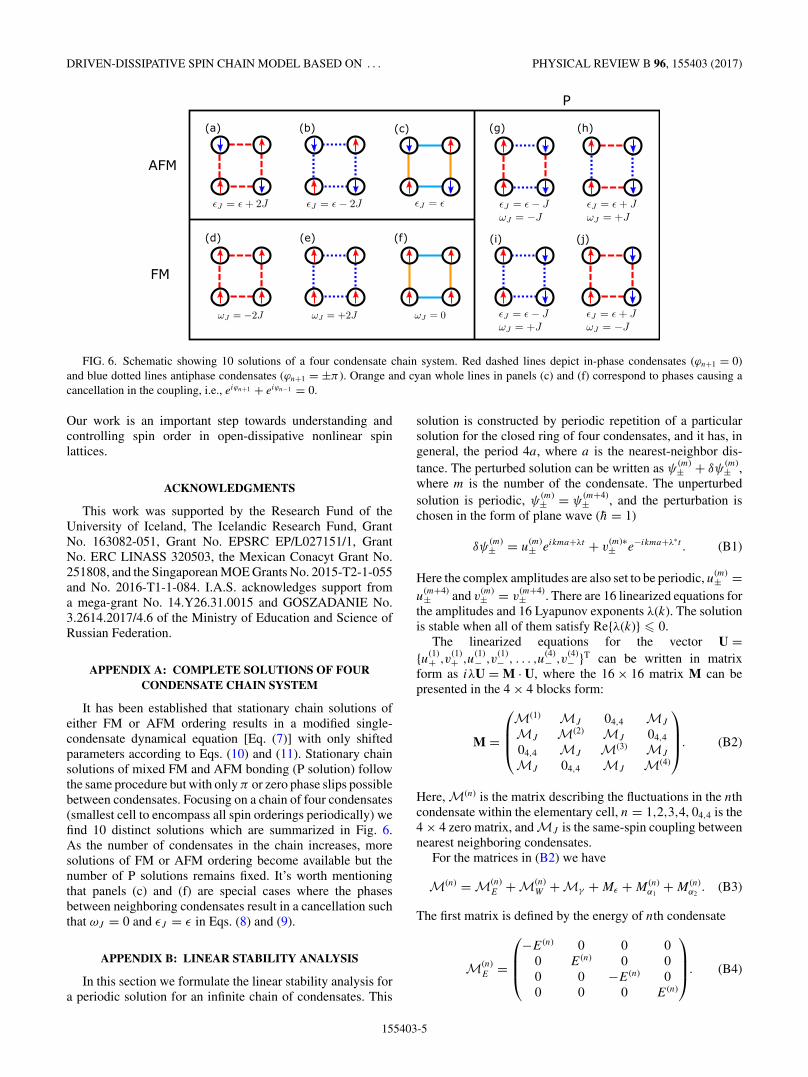
FIG. 6. Schematic showing 10 solutions of a four condensate chain system. Red dashed lines depict in-phase condensates (ϕn+1 = 0)and blue dotted lines antiphase condensates (ϕn+1 = ±π ). Orange and cyan whole lines in panels (c) and (f) correspond to phases causing acancellation in the coupling, i.e., eiϕn+1 + eiϕn−1 = 0.

Our work is an important step towards understanding andcontrolling spin order in open-dissipative nonlinear spinlattices.

ACKNOWLEDGMENTS

This work was supported by the Research Fund of theUniversity of Iceland, The Icelandic Research Fund, GrantNo. 163082-051, Grant No. EPSRC EP/L027151/1, GrantNo. ERC LINASS 320503, the Mexican Conacyt Grant No.251808, and the Singaporean MOE Grants No. 2015-T2-1-055and No. 2016-T1-1-084. I.A.S. acknowledges support froma mega-grant No. 14.Y26.31.0015 and GOSZADANIE No.3.2614.2017/4.6 of the Ministry of Education and Science ofRussian Federation.

APPENDIX A: COMPLETE SOLUTIONS OF FOURCONDENSATE CHAIN SYSTEM

It has been established that stationary chain solutions ofeither FM or AFM ordering results in a modified single-condensate dynamical equation [Eq. (7)] with only shiftedparameters according to Eqs. (10) and (11). Stationary chainsolutions of mixed FM and AFM bonding (P solution) followthe same procedure but with only π or zero phase slips possiblebetween condensates. Focusing on a chain of four condensates(smallest cell to encompass all spin orderings periodically) wefind 10 distinct solutions which are summarized in Fig. 6.As the number of condensates in the chain increases, moresolutions of FM or AFM ordering become available but thenumber of P solutions remains fixed. It’s worth mentioningthat panels (c) and (f) are special cases where the phasesbetween neighboring condensates result in a cancellation suchthat ωJ = 0 and εJ = ε in Eqs. (8) and (9).

APPENDIX B: LINEAR STABILITY ANALYSIS

In this section we formulate the linear stability analysis fora periodic solution for an infinite chain of condensates. This

solution is constructed by periodic repetition of a particularsolution for the closed ring of four condensates, and it has, ingeneral, the period 4a, where a is the nearest-neighbor dis-tance. The perturbed solution can be written as ψ

(m)± + δψ

(m)± ,

where m is the number of the condensate. The unperturbedsolution is periodic, ψ

(m)± = ψ

(m+4)± , and the perturbation is

chosen in the form of plane wave (h = 1)

δψ(m)± = u

(m)± eikma+λt + v

(m)∗± e−ikma+λ∗t . (B1)

Here the complex amplitudes are also set to be periodic, u(m)± =

u(m+4)± and v

(m)± = v

(m+4)± . There are 16 linearized equations for

the amplitudes and 16 Lyapunov exponents λ(k). The solutionis stable when all of them satisfy Re{λ(k)} � 0.

The linearized equations for the vector U ={u(1)

+ ,v(1)+ ,u

(1)− ,v

(1)− , . . . ,u

(4)− ,v

(4)− }T can be written in matrix

form as iλU = M · U, where the 16 × 16 matrix M can bepresented in the 4 × 4 blocks form:

M =

⎛⎜⎜⎝M(1) MJ 04,4 MJ

MJ M(2) MJ 04,4

04,4 MJ M(3) MJ

MJ 04,4 MJ M(4)

⎞⎟⎟⎠. (B2)

Here, M(n) is the matrix describing the fluctuations in the nthcondensate within the elementary cell, n = 1,2,3,4, 04,4 is the4 × 4 zero matrix, and MJ is the same-spin coupling betweennearest neighboring condensates.

For the matrices in (B2) we have

M(n) = M(n)E + M(n)

W + Mγ + Mε + M (n)α1

+ M (n)α2

. (B3)

The first matrix is defined by the energy of nth condensate

M(n)E =

⎛⎜⎜⎝

−E(n) 0 0 00 E(n) 0 00 0 −E(n) 00 0 0 E(n)

⎞⎟⎟⎠. (B4)

155403-5

H. SIGURDSSON et al. PHYSICAL REVIEW B 96, 155403 (2017)

The second matrix arises from the harvest and saturation rates of the condensate from the static reservoir

M(n)W = − iη

4

⎛⎜⎜⎝

2|ψ (n)+ |2 + |ψ (n)

− |2 (ψ (n)+ )2 ψ

(n)+ ψ

(n)∗− ψ

(n)+ ψ

(n)−

(ψ (n)∗+ )2 2|ψ (n)

+ |2 + |ψ (n)− |2 ψ

(n)∗+ ψ

(n)∗− ψ

(n)∗+ ψ

(n)−

ψ(n)∗+ ψ

(n)− ψ

(n)+ ψ

(n)− 2|ψ (n)

− |2 + |ψ (n)+ |2 (ψ (n)

− )2

ψ(n)∗+ ψ

(n)∗− ψ

(n)+ ψ

(n)∗− (ψ (n)∗

− )2 2|ψ (n)− |2 + |ψ (n)

+ |2

⎞⎟⎟⎠ − i

2GI, (B5)

where G = � − W and I is the identity matrix. The third and the fourth matrices arise from coupling between up and downcomponents:

Mγ = iγ

2

⎛⎜⎝

0 0 −1 00 0 0 −1

−1 0 0 00 −1 0 0

⎞⎟⎠, Mε = ε

2

⎛⎜⎝

0 0 −1 00 0 0 1

−1 0 0 00 1 0 0

⎞⎟⎠. (B6)

The fifth and the sixth matrices arise from the interactions:

M(n)α1

= α1

2

⎛⎜⎜⎝

2|ψ (n)+ |2 (ψ (n)

+ )2 0 0−(ψ (n)∗

+ )2 −2|ψ (n)+ |2 0 0

0 0 2|ψ (n)− |2 (ψ (n)

− )2

0 0 −(ψ (n)∗− )2 −2|ψ (n)

− |2

⎞⎟⎟⎠,

M(n)α2

= α2

2

⎛⎜⎜⎝

|ψ (n)− |2 0 ψ

(n)+ ψ

(n)∗− ψ

(n)+ ψ

(n)−

0 −|ψ (n)− |2 −ψ

(n)∗+ ψ

(n)∗− −ψ

(n)∗+ ψ

(n)−

ψ(n)∗+ ψ

(n)− ψ

(n)+ ψ

(n)− |ψ (n)

+ |2 0−ψ

(n)∗+ ψ

(n)∗− −ψ

(n)+ ψ

(n)∗− 0 −|ψ (n)

+ |2

⎞⎟⎟⎠. (B7)

The final matrix describes the same-spin coupling between thenearest-neighboring condensates

MJ = cos (ka)

2

⎛⎜⎝

−J 0 0 00 J ∗ 0 00 0 −J 00 0 0 J ∗

⎞⎟⎠. (B8)

APPENDIX C: NONADIABATIC MONTE CARLO FORUNDAMPED FOUR CONDENSATE CHAIN

Here we give results analogous to Fig. 3 but with dampingabsent [Im(J ) = 0] and instantaneous switching of the pumpintensity at its mark value. Unlike Fig. 3 where states withthe lowest bifurcation threshold were dominant, we uncover amore complex probability map in Fig. 7 through 30 MC trials

FIG. 7. Color maps showing the likelihood of a spin state appearing through 30 MC iterations for each pixel in a 100 × 100 map usingEq. (1). Different from Fig. 3 we get a noticeable population in three more states (FM: ωJ = 0; AFM: εJ = ε; FM: ωJ = +2J ). Black dashedlines are predicted stability boundaries calculated using Eq. (B2) for k = 0.

155403-6

DRIVEN-DISSIPATIVE SPIN CHAIN MODEL BASED ON . . . PHYSICAL REVIEW B 96, 155403 (2017)

bounded by their k = 0 stability regions (black dashed lines)predicted by Eq. (B2).

Figure 7 shows 77% of the data divided between sixsolutions of the four condensate chain. The remaining foursolutions from Fig. 6 are not observed since they are unstableover the entire J − W map. Another 11% of the data (notshown here) ended in oscillating limit cycle states discussedin Fig. 5. The remaining 12% were categorized as nonstation-ary/chaotic.

The complex features of the probability maps in Fig. 7as opposed to the more simplistic ones in Fig. 3 highlightthe important role of damping in the system and adiabaticswitching of the pump intensity. Intuitively, the complicatedfeatures in Fig. 7 arise from the order parameter overshootingmany possible stable minima in the phase space of the system.It then becomes a matter of the nearest and strongest attractorto stabilize the solution.

APPENDIX D: NUMERICAL METHODS

A QR algorithm is implemented to solve the eigenvalueproblem of Eq. (B2). Equation (1) is solved using a variable-order Adams-Bashforth-Moulton predictor-corrector method.The parameters used for 0D simulations were η = 0.02 ps−1,� = 0.1 ps−1, ε = 0.04 ps−1, γ = 0.2ε, α1 = 0.01 ps−1, α2 =−0.5α1, and Im(J )/Re(J ) = 0.1.

The parameters used for 2D simulations of Eq. (F1)were m = 5 × 10−5m0, η = 0.01 ps−1, � = 0.2 ps−1, ε =0.015 ps−1, γ = 0.2ε, α1 = 0.003 ps−1, α2 = −0.5α1, d =12 μm, σ = 10.3 μm, and � = 0.1, where m0 is the freeelectron rest mass.

APPENDIX E: DERIVATION OF THE COUPLINGCONTRIBUTION IN CHAIN SYSTEMS

Consider the stationary condensate chain composed entirelyof either FM or AFM bonds. According to Eqs. (8) and (9),each condensate with two nearest neighbors is presented witha term

ωJ = −J (eiϕi + eiϕj ), (E1)

for two FM bonds or

εJ = ε + J (eiϕi + eiϕj ), (E2)

for two AFM bonds. Here ϕi,j is the phase difference ofmoving from the condensate in question to its neighbor. Thiscontribution can in general be a complex number appearingequally in each condensate. In this section we show that thisnumber must stay real for a chain system. Note that in Eqs. (8)and (9), for the infinite chain, a phase slip from condensate n ton + 1 is written ϕn+1. Here, with four condensates periodicallyconnected, we adapt a slightly simpler notation illustratedin Fig. 8. The lattice unit cell of the chain system is onecondensate and one bond. Assuming that the chain closes onitself, the number of free variables (ϕi) is then equal to thenumber of independent equations. The following can then begeneralized to any number of condensates in a chain.

Let’s now imagine four condensates locked in a chain. Wecan classify the phase jumps going clockwise as {ϕ1,ϕ2,ϕ3,ϕ4}(see Fig. 8). It is obvious that ωJ and εJ must be equal for allcondensates in the chain in order to have a steady state. Thusthe phase contribution eiϕi + eiϕj must be the same for allcondensates. This means that the four stationary condensatesallow us to write

eiϕ1 + e−iϕ4 = eiϕ2 + e−iϕ1 = eiϕ3 + e−iϕ2 = eiϕ4 + e−iϕ3 .

(E3)

Writing eiϕi = ai + ibi , where ai,bi ∈ R, it’s then easy toshow that

a1 = a3, (E4)

a2 = a4, (E5)

b1 = b2 = b3 = b4. (E6)

The real part of the contribution eiϕi + eiϕj is thus equalfor each condensate but the imaginary part gets canceled.Consequently, from |eiϕi |2 = 1 we come to the solution a1 =∓a2, which can more clearly be written

cos (ϕ1) = ∓ cos (ϕ2). (E7)

The minus sign in Eq. (E7) corresponds to a cancellationin the coupling with no shift in ωJ or εJ , whereas theplus sign mandates the opposite. Applying the constraintei(ϕ1+ϕ2+ϕ3+ϕ4) = 1 corresponding to a full cycle in our fourcondensate chain we come to the conclusion that the onlypossible values of coupling in the latter case are cos (ϕ1) =cos (2πm/N ), where m = 0,1,2, . . . and N is the number

FIG. 8. Schematic of the four condensate chain. (Left) Phase jumps ϕi take place moving from one condensate to the next. (Middle) �1

gets a contribution eiϕ1 + e−iϕ4 . (Right) �2 gets a contribution eiϕ2 + e−iϕ1 .

155403-7

H. SIGURDSSON et al. PHYSICAL REVIEW B 96, 155403 (2017)

FIG. 9. Density and phase maps of the AFM, P, and FM spin states from Eq. (F1). Evaluating the phase difference between condensatesof dominant spin (marked with black crosses) in each solution confirms that AFM bonds favor π phase difference and FM bonds zero phasedifference.

of condensates in the chain. As the number of condensatesincreases in the chain, more solutions become available.

The same procedure can be applied to a state where eachcondensate has one FM and one AFM bond (P solutions). Thenonly eiϕi = ±1 satisfies the chain.

APPENDIX F: FOUR CONDENSATE CHAIN WITHSPATIAL DEGREES OF FREEDOM

The tight-binding model [Eq. (1)] offers a simple solutionto the stationary spin patterns in the condensate chain. Wefind that these exact solutions can also be produced withlittle difficulty accounting for the spatial degree of freedom.The complex Ginzburg-Landau equation can be written then[26,34,35]:

i� = 1

2[−i(g(S) + γ σx) + (1 − i�)

×(

αS + αSzσz − εσx − h∇2

m+ gP P (r)

)]�.

(F1)

Here, m is the effective mass of the polaritons. The excitonreservoir is taken to be completely static and the inducedrepulsive potential is then given by an effective interactionconstant gP . The remainder of the parameters serve the samepurpose here as in the tight-binding model with W = P (r). Wenote that modeling the system by coupling an exciton reservoirrate equation to the order parameter only requires rescalingof the parameters and does not critically affect the observedsolutions in Eq. (F1) when the decay rate of the reservoir istaken to be large compared to the polariton lifetime [36].

The pump P (r) is a 3 × 3 square arrangement of Gaussiansseparated by the lateral distance d and with a FWHM σ whichthen form a four potential minimum in a 2 × 2 arrangementwhere the polaritons condense. In Fig. 9 we show threesolutions of different spin order in a closed four condensatechain. The AFM, P, and FM solutions possess phase slipscorresponding to the lowest bifurcation threshold solutionsfrom Figs. 6(b), 6(d) and 6(g), and Figs. 3(a)–3(c). Eachsolution can be achieved by either tuning the strength ofpolariton interaction with the pump gP , or by increasing thestrength of the center Gaussian pump spot causing an increasedbarrier between the condensates which effectively changes thecoupling strength J .

[1] J. Hopfield and D. Tank, Science 233, 625 (1986).[2] N. N. Vtyurina, D. Dulin, M. W. Docter, A. S. Meyer, N. H.

Dekker, and E. A. Abbondanzieri, Proc. Natl. Acad. Sci. USA113, 4982 (2016).

[3] D. L. Stein and C. M. Newman, Spin Glasses and Complexity(Princeton University Press, Princeton, NJ, 2013).

[4] J.-P. Bouchaud, J. Stat. Phys. 151, 567 (2013).[5] K. Kim, M.-S. Chang, S. Korenblit, R. Islam, E. E. Edwards,

J. K. Freericks, G.-D. Lin, L.-M. Duan, and C. Monroe, Nature(London) 465, 590 (2010).

[6] H. Diep, Frustrated Spin Systems (World Scientific, Singapore,2013).

155403-8

DRIVEN-DISSIPATIVE SPIN CHAIN MODEL BASED ON . . . PHYSICAL REVIEW B 96, 155403 (2017)

[7] C. Nisoli, R. Moessner, and P. Schiffer, Rev. Mod. Phys. 85,1473 (2013).

[8] J. Drisko, T. Marsh, and J. Cumings, Nat. Commun. 8, 14009(E)(2017).

[9] J. A. Katine, F. J. Albert, R. A. Buhrman, E. B. Myers, andD. C. Ralph, Phys. Rev. Lett. 84, 3149 (2000).

[10] M. M. Glazov and A. V. Kavokin, Phys. Rev. B 91, 161307(2015).

[11] J. Stenger, S. Inouye, D. M. Stamper-Kurn, H.-J. Miesner, A. P.Chikkatur, and W. Ketterle, Nature (London) 396, 345 (1998).

[12] T. C. H. Liew, A. V. Kavokin, and I. A. Shelykh, Phys. Rev.Lett. 101, 016402 (2008).

[13] C. Adrados, T. C. H. Liew, A. Amo, M. D. Martín, D. Sanvitto,C. Antón, E. Giacobino, A. Kavokin, A. Bramati, and L. Viña,Phys. Rev. Lett. 107, 146402 (2011).

[14] M. Mezard, G. Parisi, and M. A. Virasoro, Spin Glass Theoryand Beyond (World Scientific, Singapore, 1986).

[15] A. Le Boité, G. Orso, and C. Ciuti, Phys. Rev. Lett. 110, 233601(2013).

[16] N. G. Berloff, K. Kalinin, M. Silva, W. Langbein, and P. G.Lagoudakis, arXiv:1607.06065 [cond-mat.mes-hall].

[17] T. Inagaki, K. Inaba, R. Hamerly, K. Inoue, Y. Yamamoto, andH. Takesue, Nat. Photon. 10, 415 (2016).

[18] M. D. Fraser, S. Hofling, and Y. Yamamoto, Nat. Mater. 15,1049 (2016).

[19] T. Liew, I. Shelykh, and G. Malpuech, Phys. E (Amsterdam,Neth.) 43, 1543 (2011).

[20] D. Sanvitto and S. Kena-Cohen, Nat. Mater. 15, 1061 (2016).[21] B. Nelsen, G. Liu, M. Steger, D. W. Snoke, R. Balili, K. West,

and L. Pfeiffer, Phys. Rev. X 3, 041015 (2013).[22] H. Ohadi, A. Dreismann, Y. G. Rubo, F. Pinsker, Y. del Valle-

Inclan Redondo, S. I. Tsintzos, Z. Hatzopoulos, P. G. Savvidis,and J. J. Baumberg, Phys. Rev. X 5, 031002 (2015).

[23] K. V. Kavokin, I. A. Shelykh, A. V. Kavokin, G. Malpuech, andP. Bigenwald, Phys. Rev. Lett. 92, 017401 (2004).

[24] H. Ohadi, Y. del Valle-Inclan Redondo, A. Dreismann, Y. G.Rubo, F. Pinsker, S. I. Tsintzos, Z. Hatzopoulos, P. G.Savvidis, and J. J. Baumberg, Phys. Rev. Lett. 116, 106403(2016).

[25] H. Ohadi, A. J. Ramsay, H. Sigurdsson, Y. del Valle-InclanRedondo, S. I. Tsintzos, Z. Hatzopoulos, T. C. H. Liew, I. A.Shelykh, Y. G. Rubo, P. G. Savvidis, and J. J. Baumberg,Phys. Rev. Lett. 119, 067401 (2017).

[26] J. Keeling and N. G. Berloff, Phys. Rev. Lett. 100, 250401(2008).

[27] P. Stepnicki and M. Matuszewski, Phys. Rev. A 88, 033626(2013).

[28] L. Kłopotowski, M. Martín, A. Amo, L. Viña, I. Shelykh, M.Glazov, G. Malpuech, A. Kavokin, and R. André, Solid StateCommun. 139, 511 (2006).

[29] R. Balili, B. Nelsen, D. W. Snoke, R. H. Reid, L. Pfeiffer, andK. West, Phys. Rev. B 81, 125311 (2010).

[30] I. L. Aleiner, B. L. Altshuler, and Y. G. Rubo, Phys. Rev. B 85,121301 (2012).

[31] M. Wouters and V. Savona, Phys. Rev. B 79, 165302(2009).

[32] D. Read, T. C. H. Liew, Y. G. Rubo, and A. V. Kavokin, Phys.Rev. B 80, 195309 (2009).

[33] K. Rayanov, B. L. Altshuler, Y. G. Rubo, and S. Flach, Phys.Rev. Lett. 114, 193901 (2015).

[34] M. Wouters and I. Carusotto, Phys. Rev. Lett. 99, 140402(2007).

[35] M. Wouters, T. C. H. Liew, and V. Savona, Phys. Rev. B 82,245315 (2010).

[36] L. A. Smirnov, D. A. Smirnova, E. A. Ostrovskaya, and Y. S.Kivshar, Phys. Rev. B 89, 235310 (2014).

155403-9