Drinking and Driving and Public Transportation:

A Test of the Routine Activity Framework

by

Joshua Broyles

A Thesis Presented in Partial Fulfillment

of the Requirements for the Degree

Master of Science

Approved April 2014 by the

Graduate Supervisory Committee:

Justin Ready, Chair

Cody Telep

Michael Reisig

ARIZONA STATE UNIVERSITY

May 2014

i

ABSTRACT

Driving under the influence (DUI) is a problem in American society that has

received considerable attention over recent decades from local police agencies, lobby

groups, and the news media. While punitive policies, administrative sanctions and

aggressive media campaigns to deter drinking and driving have been used in the past, less

conventional methods to restructure or modify the urban environment to discourage

drunk driving have been underused. Explanations with regard to DUIs are policy driven

more often than they are guided by criminological theory. The current study uses the

routine activities perspective as a backdrop for assessing whether a relatively new mode

of transportation – an urban light rail system – in a large metropolitan city in the

Southwestern U.S. can alter behaviors of individuals who are likely to drive under the

influence of alcohol. The study is based on a survey of undergraduate students from a

large university that has several stops on the light rail system connecting multiple

campuses. This thesis examines whether the light rail system has a greater effect on

students whose routines activities (relatively unsupervised college youth with greater

access to cars and bars) are more conducive to driving under the influence of alcohol. An

additional purpose of the current study is to determine whether proximity to the light rail

system is associated with students driving under the influence of alcohol, while

controlling for other criminological factors

ii

DEDICATION

This thesis is dedicated to the faculty of Arizona State University, who never set a

limit to what I could accomplish. It is dedicated to my peers in the School of Criminology

and Criminal Justice, who kept me focused and provided a solid learning environment

wherein I could flourish. It is further dedicated to the soldiers of the 860th

Military Police

Company, who reminded me that academia, while important, isn’t everything; to my

friends who have kept me sane throughout the years; finally, to my family, who never

gave me a path to follow, but instead gave me the tools to find my own way.

iii

TABLE OF CONTENTS

Page

LIST OF TABLES .................................................................................................................... v

LIST OF FIGURES ................................................................................................................. vi

CHAPTER

1 INTRODUCTION ................. .............................................................................. 1

2 DRUNK DRIVING AND PUBLIC TRANSPORTATION ............................... 3

College drinking ......................................................................................... 7

Prior research .............................................................................................. 8

3 ROUTINE ACTIVITIES AND DRUNK DRIVING .......................................... 9

4 SELF-CONTROL AND DRUNK DRIVING ................................................... 12

5 HYPOTHESES ................... ............................................................................... 14

6 METHODS ...................... .................................................................................. 15

Survey instrument .................................................................................... 17

Control variables ...................................................................................... 19

Independent variables .............................................................................. 21

Dependent variables ................................................................................. 21

Analytic strategy ...................................................................................... 22

Limitations................................................................................................ 24

7 RESULTS ...................... ..................................................................................... 24

8 DISCUSSION ................... ................................................................................. 28

REFERENCES....... .............................................................................................................. 33

iv

APPENDIX

A Correlation Matrix ................................................................................................ 42

B Binge Drinking Logistic Regression ................................................................... 44

v

LIST OF TABLES

Table Page

1. Descriptive Statistics from Drinking and Phoenix Transportation use survey .... 23

2. Binge Drinking Negative Binomial Model ......................................................... 26

3. Drinking and Driving Logistic Regression ........................................................... 27

vi

LIST OF FIGURES

Figure Page

1. Valley Metro Public Transit Map .................................................................... 4

2. Valley Metro Light Rail Map .......................................................................... 5

3. Do Students Consider Using the Light Rail After Drinking ........................ 25

4. Would Expanding the Light Rail Reduce Drinking and Driving ................. 25

1

INTRODUCTION

Crime statistics and self-report data show that college students are one of the most

likely groups to drive intoxicated (Nagin, & Paternoster, 1993; Cohen, 1990). Drunk

driving has been a notable scourge in recent American history. In Arizona specifically,

28% of fatalities on streets and highways in 2009 were linked to drunk driving (National

Highway Traffic and Safety Administration, 2010). Since the establishment of highly

visible advocacy and lobby groups in the 1980s, such as Mothers Against Drunk Driving

(MADD), the public health problem of drunk driving has been a concern of those

responsible for public safety. Likewise, MADD has influenced lawmakers to “crack

down” on drunk driving, and they have facilitated the development of other subsidiary

organizations that have taken up the cause of discouraging and sanctioning DUIs, such as

Students Against Drunk Driving (SADD) (Wooster, 2000).

Recently, as of December 2008, an inner city light rail system was implemented

in the Phoenix metropolitan area to provide a broader network of alternative public

transportation routes and to connect the cities of Phoenix, Tempe, and Mesa. Tempe and

downtown Phoenix house the Arizona State University (ASU) campuses, as well as

densely populated drinking areas near both campuses and several college and

professional sports arenas. Furthermore, it has been established that most DUI arrests

take place as motorists are returning from a licensed drinking location (Helander, 2002;

Shults et al. 2001; O’Donnell, 1985). Because of this fact, it is important to investigate

whether building and operating a new light rail system in these areas changes students’

“routine activities” as they relate to drinking and driving. Does giving this population of

2

ASU students a relatively cost effective alternative to driving while intoxicated change

their routine activities and make them more likely to use the safer alternative? And if the

new transportation system does affect student behavior, do certain students benefit more

from the light rail system (i.e., students whose routine activities are more conducive to

driving impaired)? On the other hand, will college students maintain their normal activity

patterns and drive to and from drinking establishments while intoxicated despite the new

light rail system?

It is also helpful to draw from the routine activities perspective as a theoretical

backdrop to investigate what lifestyle and activity patterns are associated with driving

while intoxicated. For instance, to what extent does proximity to the light rail system

affect drinking and driving? How does access to alcohol and alternative modes of

transportation affect students’ self-reported drunk driving patterns? And to what degree

does unsupervised time and social attachments (i.e., intimate handlers) affect DUI risk

taking behavior? It is important to gather this information because there are notable

policy implications if the light rail system shows a reduction in drunk driving among

certain subgroups of college students. First, it will represent a potential reduction in the

loss of life and property damage attributed to drunk-driving accidents in the greater

Phoenix area. Second, other municipalities could capitalize on this research and

encourage high-risk individuals to take advantage of public transportation systems.

Further, it may be useful to eventually extend the light rail lines into the Phoenix

metropolitan area so that a greater segment of the resident population can benefit from

proximity to the light rail as well. To date, while studies suggest that using public

3

transportation reduces DUI offenses (see Wiliszowski, Murphy, Jones, & Lacey, 1996;

Grohosky, Moore, & Ochshorn, 2007), the amount of literature focusing on the effects of

public transportation on DUI is limited. This thesis builds upon this literature.

DRUNK DRIVING AND PUBLIC TRANSPORTATION

A substantial amount of legislation has focused on the deterrence of drunk driving

by increasing criminal and administrative penalties for intoxicated drivers, but the logic

of increasing punitive sanctions for driving impaired may be flawed. For example, state-

level legislation has attempted to impose steep fines, jail time, shaming practices, license

revocation, ignition interlock devices and zero tolerance practices (Ornstein, & Hanssens,

1985; Shore & Maguin, 1988; Carpenter, 2003; Raub, Lucke & Warke, 2003). While

these statutes have created harsher penalties and have been paired with aggressive

campaigns to make it known that it is not prudent to drive impaired, they have not

provided alternatives to driving under the influence of alcohol. Suggested alternatives

include using a designated driver, taking a cab, or simply not drinking to the point of

intoxication. These alternatives, however, may not be practical in the mind of likely

offenders. A cab ride may be expensive depending on income and where the individual

lives, and it is a social taboo to call a friend in the middle of the night while one is

intoxicated (Grohosky, Moore, & Ochshorn, 2007; Pratt & Reisig, 2011). Furthermore, it

may be seen as inconvenient to individuals who feel they cannot rely on friends or family

to pick them up. A designated driver is more practical and cheaper, but some research

shows that designated drivers are still likely to drink in social atmospheres, despite

serving the role of the designated driver (Helander, 2002; Timmerman, Geller,

4

Glindeman, Fournier, 2003). For example, Timmerman et al. (2003) found that

designated drivers typically abstain from drinking more than non-designated drivers, but

their average blood alcohol content was still .06, which is barely under the legal limit in

most states. In fact, in the state where the current research was conducted, an individual

can still be charged with a DUI if their blood alcohol content is over .05 (Arizona

Revised Statutes 28-1381.1, 2007).

Figure 1 Valley Metro Public Transit Map (Valley Metro, 2013)

Key for Fig 1: =Light rail line

With respect to mobility in the Phoenix metropolitan area, a more reliable

alternative to driving intoxicated is public transportation, such as the bus system. Taking

the bus, however, may be complicated for some individuals who are not familiar with bus

routes, who are intimidated by using the transportation system, or who are fearful for

their safety at night or in certain neighborhoods. This complication is illustrated in a map

5

of the bus system in the Phoenix metropolitan area (see Figure 1). According to Valley

Metro, there are over 90 different bus routes in the greater Phoenix area. These routes are

complicated by the times at which each bus arrives and the direction each bus travels. In

fact, lack of knowledge and availability of public transportation has been cited as a major

reason for driving drunk or without a license (Ross & Gonzales, 1988). The light rail

system, on the other hand, may still be intimidating, but is arguably easier to understand

and use given that there is only one line, and the light rail stops at every platform roughly

every 10 to 20 minutes (Valley Metro, 2011). The map of the light rail is presented in

Figures 1 and 2.

Figure 2 Valley Metro Light Rail Map (Valley Metro, 2013).

Key for Fig. 2: =ASU Campuses. = Heavy drinking locations.

In December 2008, the light rail system was opened to the public in Phoenix,

Tempe and Mesa (Náñez, 2008). Originally, the concept of a light rail was not as well-

accepted in cities such as Phoenix because of the hot, dry weather. Early in the city’s

history a small trolley system did exist. It consisted of approximately 12 miles of track

6

that crisscrossed the downtown area and 17 additional miles of tracks that reached into

the suburbs. This trolley system began running in 1887 before the advent of buses and it

was originally powered by mules and horses. It continued to expand with the use of

electric motors but ceased running in 1948 after a carbarn fire destroyed 12 of 18 trolley

cars. This carbarn fire inadvertently made way for the new, more technologically

advanced buses already being put in use, and by 1948 there was no need to further invest

in the rail system (Fleming, 1977).

The hot, dry summers had continued to make it unsuitable for Phoenix to invest

heavily in a more extensive public transportation system because the general public

would be discouraged from waiting for long periods of time in the heat for their bus or

train (Kuby, Barranda, & Upchurch, 2004). To overcome this obstacle, city planners

developed shortened waiting times and the provision of structures that created shade at

light rail platforms in order to make riding the light rail and its 28 two-directional stops

more practical (Valley Metro, 2011; Kuby, et al., 2004). Furthermore, light rail systems

are useful for moving large populations to and from central business districts. Because

the Phoenix metropolitan area has a population distributed across 16,573 square miles,

the light rail became a more worthwhile project from a city planning perspective (Joshi,

Guhathakurta, Konjevod, Crittenden & Li, 2006; Kuby et al, 2004). Additional public

benefits of a light rail include the improvement of air quality, reduction of traffic

congestion, increased property value around the light rail, as well as an influx of

employment opportunities. With seven stops near ASU campuses and reduced prices for

students, the light rail system is made even more accessible to students (Valley Metro,

7

2011; Arizona State University, 2012). This paper intends to further research the potential

benefits of the light rail in Phoenix by testing the association between use of and

proximity to the light rail and drunk driving among the ASU student population.

College Drinking

College students have higher rates of DUI than many other demographic groups.

This is due, in part, to the fact that the most frequent offenders of drunk driving are

between the ages of 18 and 24 (Stewart, 2008; McCartt, Hellinga, & Wells, 2008).

Additionally, college students have been shown to be more dangerous than their non-

college counterparts while drinking and driving due to binge drinking that frequently

occurs on college campuses (Robertson & Marples, 2008). In addition to being a

subpopulation at a more likely age for driving intoxicated (Stewart, 2008) college

students routinely participate in social drinking activities (Clapp, Johnson, Voas,

Shillington, Lenge, & Russel, 2005; Fisher, Sloan, Cullen, & Lu, 1998). Even when

drinking and driving is taken out of the equation, drinking on its own routinely causes

social and health-related problems on college campuses. Drinking games and a

competitive drinking environment result in more frequent victimizations, including

sexual assaults and theft, as well as a greater propensity for aggression, violence, and

other crimes (Fisher et al., 1998; Zhang, Wieczorek, & Welte, 1997). Fortunately, it has

been demonstrated that campaigns to curb drunk driving have a considerable effect on

college students at the target age of 18-24 (McCartt, Hellinga & Wells, 2008). According

to ASU’s demographic profile, as of 2009 82% of the undergraduate population was

under the age of 25 which, all things considered, makes it an ideal target population for

8

this study (2010). Given the above information, this thesis intends to capitalize on the fact

that college students are typically at a higher risk for drinking and driving due to their

propensity to binge drink. This study will investigate if there is an association between

binge drinking and light rail use.

Prior Research

One of the few studies to investigate the effects of a rail system on drinking and

driving was conducted in Washington, DC by Jackson and Owens (2011). Washington,

DC’s metro system is a more extensive system of rail networks relative to the size of the

light rail in Phoenix. It is concentrated in the center of the Washington, DC and extends

outbound in multiple directions into the neighboring states of Maryland and Virginia. The

DC Metro comprises five lines and 86 unique stops. Prior to 1999, the DC rail system

ran its last trains from the center of the city out bound at midnight. However, in

November 1999, the metro remained open an additional hour on Fridays and Saturdays

with the intent of catering to college students from the University of Maryland, George

Washington University, American University, George Mason University, and

Georgetown University who were likely to be in DC to socialize and congregate at

popular restaurants and drinking locations. After finding an increase in ridership during

the extended time period, the DC metro system again extended the late night hours to

2:00 am on Fridays and Saturdays (technically Saturday and Sunday mornings) in 2000.

Finally, in 2003 city administrators changed the final departure time to 3:00 am for the

last train leaving central DC (Jackson & Owens, 2011). Jackson and Owens capitalized

on these schedule changes which provided a natural experiment to examine whether

9

drunk driving arrest rates and accidents in the DC area were reduced as a result of the

operating time changes. Furthermore, they tested whether the distance a bar is from a

metro station stop affected the rate at which citizens are arrested for DUI in that area.

That analytic approach provides the framework for this study.

While Jackson and Owens found that the metro exerted no direct effect on general DUI

arrest rates and drunk driving accidents, spatial analyses showed a positive association.

That is, the proximity to a drinking establishment was correlated with lower DUI arrest

rates. In addition, neighborhoods with a bar within 100 meters of a metro station stop had

a 14% reduction in DUI arrest rates (Jackson & Owens, 2011). This suggests that a

relationship exists between distance traveled to drinking establishments and access to

public transportation. It is important to reiterate that one of the main reasons for

extending the train hours was attributed to college students socializing and drinking

alcohol. Therefore, though it was not captured in the data, it is possible that the lower rate

of DUIs was a result of less drunk driving by college students.

ROUTINE ACTIVITIES AND DRUNK DRIVING

Studies linking criminological theory to drinking among college student

populations are not new (See Lanza-Kaduce, 1988; Durkin, Wolfe, & Clark, 1999). Most

theories, however, have focused on the effects of drinking on being victimized or

committing predatory crimes. Many of these studies are guided by theories of rational

choice and routine activities (Fisher et al., 1998; Lauritsen, Sampson, & Laub, 1991).

Cohen and Felson (1979) explained that crime exists, in part, because a person’s daily

routines occur in a social environment where crime is able to thrive. The theory is often

10

used to describe patterns of victimization and predatory crimes, and it does not typically

explain criminality or criminal motivation (Cohen & Felson, 1979; Sherman, Gartin, &

Buerger, 1989; Holtfreter, Reisig & Pratt, 2008). It assumes, rather, that criminal

motivations already exist, especially among certain subgroups of the population. As

Felson and Cohen stated in their paper on the ecology of crime, their study takes

criminality“…as given and examines how social structure allows people to translate their

criminal inclinations into action. [They] treat criminal violations as routine activities

which share many attributes of and are interdependent with other activities” (1980, p.

390). Even though the present study is examining binge drinking and drunk driving, both

non-predatory acts of deviance, routine activities theory is still an applicable framework

for examining the distribution of DUIs around the college community and light rail

system. Indeed, according to the theory, changes in technology – specifically

transportation and communication – are seen as seminal processes that impact the

convergence of likely offenders and suitable targets in the absence of capable

guardianship.

It is expected that young people may experience the urge or motivation to drink

and drive (Gruenewald, Mitchell, & Treno, 1996; Gruenewald, Johnson & Treno, 2002).

This is the result of two intersecting social patterns. People over the age of 21 congregate

at establishments where alcohol is sold legally, and people in large sprawling cities like

Phoenix and LA must routinely drive to locations of interest and necessity. It is, of

course, reasonable to assume that drinkers will still want to have mobility despite being

intoxicated, so will therefore be tempted to drive after drinking. Social structures –both

11

formal and informal – have contributed to the elements necessary for an individual to

drive under the influence of alcohol. This partly explains why drunk driving is relatively

commonplace, and in fact only about 1 in 200 to 1 in 1,500 drunk drivers on the road are

ever arrested (Kingsnorth, 1993; Vinglis, Adlaf, & Chung, 1982).

As previously shown, however, municipalities and criminal justice agencies have

attempted to create a level of deterrence in relation to drinking and driving via harsh

criminal sanctions (Ornstein, & Hanssens, 1985; Carpenter, 2003). While formal criminal

sanctions exist against mainstream crimes like burglary and motor vehicle theft, there are

also informal, situational crime prevention techniques that empower citizens to

discourage motivated offenders from pursuing these crimes. In the case of conventional

crimes like theft, if efforts to “harden” targets, reduce access and increase natural

surveillance around targets are used, offenders should be less tempted to engage in the

crime because of change in the opportunity structure (Felson & Cohen, 1979; Clarke,

1995). Additionally, despite the fact that society has favorable views toward harsh

punishments for drunk driving, the threat of sanctions alone do not contribute to decision

making with regard to drinking and driving (Applegate, Cullen, Link, Richards, & Lanza-

Kaduce, 1996; Schell, Chan, & Morral, 2006).

Furthermore, it has been shown that methods for deterrence are not as salient as

they were once believed to be (Lanza-Kaduce, 1988; Pratt & Cullen 2005; Pratt, Cullen,

Blevins, Daigle & Madensen, 2008). If fines and jail time do not deter drunk driving,

how then can private citizens play a role in reducing the magnitude of this problem?

Since the consumption of alcohol is legal for those over the statutory age limit,

12

opportunity reducing techniques and situational diversions are not always feasible.

Advisory campaigns use publicity to admonish individuals to use a designated driver, or

taking away the keys of an impaired driver (Shore & Maguin, 1988; Wiliszowski,

Murphy, Jones, & Lacey, 1996). These methods, however, are sometimes idealistic as

they are ineffective for younger, high-risk segments of the population (Adebayo, 1988;

Timmerman et al., 2003). This demonstrates the primary difference between preventing

drunk driving and other consensual crimes as opposed to controlling predatory crimes;

there is a greater onus on encouraging the potential offender to play an active role in

preventing the criminal act from occurring. This makes the rational decision making

process particularly important.

The most important aspect about rational choice theory is that decisions and

information play a pivotal role in how the criminal act is planned and executed (Clarke,

1995). In the instance of drunk driving, the likely offender must know his or her options –

or the choice structuring properties associated with the act – and make a decision

according to the anticipated costs and benefits of potential outcomes. Based on the

rational choice framework, the offender’s decision making process is “bounded” or

limited by time constraints surrounding the criminal opportunity, the availability of

information, and the cognitive state of the individual. These limitations are particularly

salient for thinking about and designing alternatives for DUI offenders. Jackson and

Owens (2011) referred to this as the “safer option” which is defined as giving people a

chance to opt out of committing crimes. This is where alternative public transportation

options may come into play. If there is an inexpensive and easily accessible method of

13

public transportation, and it can fulfill the impaired person’s primary motivations –

getting to their destination quickly – then the intoxicated person may avoid driving under

the influence of alcohol, particularly in high risk areas such as college campuses, instead

opting to use the light rail system to reach their destination.

SELF-CONTROL AND DRUNK DRIVING

Self-control is an important element in the DUI offender’s decision making

process with regard to use of the light rail system. Self-control theory argues that

individuals with low levels of self-control are more likely to be short sighted, risk

seeking, prefer immediate gratification to long-term goals, and have an inability to self-

regulate their behavior (Gottfredson & Hirschi, 1990). This predisposition has been

shown to be a precursor to criminal and deviant behaviors (Pratt & Cullen, 2000). It

follows that individuals with low self-control would have a greater inclination toward

drinking and driving (Keane, Maxim, & Teevan, 1993; Piquero, & Tibbetts, 1996).

Because those with low self-control tend to be short sighted, however, the theory would

predict that these individuals are also less likely to plan ahead to use the light rail system.

If, however, the light rail schedule and stop locations become familiar to city dwellers,

and the rail becomes an integral part of how people move about the city, low self-control

may be offset by the familiarity, easy and patterned use of the light rail system. It is also

likely that many people (i.e., students) who are impaired will still rely on the light rail,

despite not planning ahead - particularly if they are familiar with, and fear, the risks and

penalties associated with driving under the influence of alcohol. In essence the light rail

may still be a viable option to those with low levels of self-control even after the point of

14

inebriation. It follows that it is necessary to measure this control variable in order to test

whether opportunities to restructure student’s routine activity patterns outweigh the

effects of low self-control (Piquero & Tibbetts, 1996; Tibbetts & Myers, 1999; Wright,

Caspi, Moffitt, & Paternoster, 2004).

Within the framework of this study, one possibility is that self-control is a

depletable resource, comparable to a muscle (Baumeister, 2002; Baumeister &

Heatherton, 1996). While Baumeister (2002) contends that there are many ways that an

individual’s self-control may be depleted, it is important to note specifically, that this

process of depletion often leads to alternative forms of criminal and deviant behaviors

(Muraven, Pogarsky, & Shmueli, 2006). Additionally, alcohol has the ability to be the

catalyst to self-control depletion (Baron & Dickerson, 1999; Fillmore & Vogel-Sprott,

1999; Muraven, Collins & Nienhaus, 2002). This is important because it is possible there

will be a compounding effect. Those who have low self-control are more likely to binge

drink, which in turn triggers more deviant behaviors such as an increased likelihood of

driving under the influence of alcohol (Baumeister & Heatherton, 1996; Piquero, Gibson

& Tibbetts, 2002; Gibson, Schrek & Miller, 2004). Considering this potential outcome,

self-control may be particularly influential in this study. While routine activities are

modifiable, those individuals with low self-control and a predisposition to drink

excessively may be less inclined to take advantage of the light rail system. Accordingly,

the survey instrument includes measures of binge drinking in addition to measurements

of self-control and self-reported drunk driving.

15

HYPOTHESES

The purpose of this research is to determine whether the existence of the light rail

system in the Phoenix Metro area is associated with self-reported drunk driving among

ASU students. Furthermore, the author attempts to discover if student binge drinking is

predicted by use of and proximity to the light rail. It is anticipated that the light rail will

be associated with student binge drinkers because those students will find it easier to

drink to excess, since they have guaranteed transportation home. Therefore, it is

additionally expected that the light rail will be associated with reduced frequency of

drunk driving among the sample of ASU students. Tests of these hypotheses would serve

as a first step in demonstrating that the light rail alters student routine activities.

Moreover, there is also an expectation that those who live close to the light rail system

are less likely to drive intoxicated than students who do not live in close proximity to the

rail. Finally, it is suspected that these effects will remain, even after controlling for self-

control and routine activities that are conducive to driving under the influence of alcohol.

Stated formally, the hypotheses tested in this study are as follows:

1) A positive relationship will exist between frequency in which ASU students

use the light rail system and their self-reported binge drinking activity.

2) A significant negative relationship will exist between the frequency in which

ASU students use the light rail system and their self-reported DUI activity.

3) A significant negative relationship will exist between residential proximity to

the light rail system and self-reported drunk driving.

16

4) Use of, and proximity to, the light rail system will be positively associated

with students binge drinking, even after controlling for self-control, social

learning, and routine activity patterns.

5) Use of, and proximity to, the light rail system will be negatively associated

with drunk driving, even after controlling for the effects of self-control, social

learning, and routine activity patterns.

METHODS

A cross-sectional research design was used to answer the above questions by

surveying 563 undergraduate students at ASU in addition to 50 online students. A total of

93.5% of students who were administered the survey responded to the survey creating a

sample size of 573 undergraduate students. Each hard copy survey was entered into the

corresponding online program, Qualtrics, in order to ensure the answers were coded

consistently.1 Students were surveyed on both the West campus in west Phoenix and the

downtown campus located in south Phoenix. While the main body of students surveyed

(539 students) were surveyed at the downtown campus, the large size and sprawling

nature of the Phoenix metropolitan area allowed for a great dispersion of students.

Therefore the sample population is composed of 37.2% of respondents who live less than

a mile from the light rail, and 54.1% who live further than 2 miles from the light rail.2

Students were included in the sampling frame and solicited to participate in the

survey based on a two stage process. First, the author selected a convenience sample of

1Qualtrics is a web based platform that allows for the survey to be created in topical sections each answer

provides for a precoded response. Additionally, the system allows for steps to be taken to ensure that the IP

addresses from which the online students submit the survey are not visible to the authors or any other

parties 2 The remaining 8.7% of students reported living between 1 and 2 miles from the light rail.

17

17 classes3 from the two previously mentioned campuses using known contacts who were

teaching during the testing period. The instructors were informed of the study and the

corresponding survey and asked if they would allow the author to survey the classes

during the first 20 minutes of the period. Since the greatest risk of drunk driving is posed

by people who are returning home from bars (Shults et al., 2001; O’Donnell, 1985),

classes that were at the 300 level or higher were targeted for selection to increase the

chances of students being at least 21 years of age. This study is cross-sectional, so the

behaviors and attitudes of students will be captured only at the point in time when the

survey is completed. In an attempt to increase response rates, the respondents were given

the opportunity to enter their email address into a raffle for a pair of headphones.4

Survey Instrument

The survey instrument contained 90 items organized within 9 topic areas.5 Many

items were adapted from previous survey instruments such as a 13 point scale measuring

self-control from Tangney, Baumeister, & Boone (2008) in addition to questions

regarding alcohol use from the Harvard College Alcohol Survey (CAS) (Wechsler,

1997). Due to the specific nature of this research, however, most items were created by

the author in a straightforward attempt at gathering the necessary information about the

variables from the respondents. Furthermore, in some instances multiple variations of

questions were asked to ensure reliability of the survey items. For instance, “Do you

3 15 of the 17 classes surveyed were criminal justice courses, therefore this survey was primarily guided by

students in criminal justice classes. The remaining 2 classes were philosophy classes. 4In addition to the raffle, 3 professors offered their students extra credit for participating in the survey. This

was done independent from any requests by the author. 5The 9 topic areas respectively were self-control, drinking behaviors, drinking and driving behaviors, use of

transportation, frequency of use and proximity to the light rail, drinking routines (places, days and times),

beliefs regarding the light rail, and demographical questions.

18

believe you live within reasonable distance from the light rail?”; “About how many

minutes would it take you to walk to the nearest light rail stop from home?” and “About

how far from the light rail do you live?” were all questions that measured proximity to

the light rail.6 It is also worth noting that several other situational measures were

considered. These measures included whether or not the light rail system is accessible, if

the rail was used at all by the individual (regardless of whether or not they had been

consuming alcohol) and if so how often was it used.

The hard copy of the survey instrument provided no legitimate skip questions;

therefore, respondents saw and answered all of the items appropriately. Because the

survey focuses on drinking behaviors and 15.4% of students (88 students) indicated

abstaining from alcohol in the past year, a N/A response was provided for a majority of

the questions. This aided the author in two ways. First, because the survey was done in a

large group setting, providing a N/A option slowed down the respondents who did not

drink. This helped to avoid drinkers and non-drinkers from self-identifying themselves to

their peers as they turned in the survey. Second, it provided extra context to some

responses. For example, a person who indicates that they have had a DUI in the past and

marks N/A on owning, borrowing and renting a vehicle likely has had their license

suspended.

In the online survey, however, one contingency question caused a skip pattern to

occur. If the respondent did not indicate that they had consumed alcohol in the past year,

their survey skipped most questions relating to alcohol consumption. To keep the data

6 The survey attached in the appendix section illustrates the response options to these questions.

19

and responses consistent, the hard copy surveys were entered into the online survey

manually by the author. Self-control measures, demographic information and

transportation use were still recorded using the software, however.

Control Variables

Demographics. Basic demographic information was collected from the sample.

The information relevant to the analysis is as follows: age, gender (male = 1; female = 0),

race (0 = white; 1 = nonwhite). Additional demographics were recorded and are

discussed in the following section on routine activities measurements since the variables

appropriately measure guardianship.

Measures of Routine Activities. A major group of control variables in this study

relate to routine activities conducive to drunk driving. More specifically, it is reasonable

to expect that individuals who have routine activities that are conducive to, or facilitate,

DUI will report driving under the influence of alcohol more frequently. Accordingly,

guardianship is measured by how much time in a typical day the respondent is supervised

– or in the presence of family members, teachers, or supervisors at work. The options for

this were measured using employment (0 = unemployed; 1 = employed), time spent with

family,7 and how many credit hours a student is enrolled in.

8 Access to suitable targets is

measured by identifying alcohol consumption, specifically with regard to binge drinking.

Additionally three simple yes/no items were asked to obtain access to personal

transportation. Does the respondent own a car, do they have access to a car that could be

7Time spent with family was categorized and coded from 0-5; respectively the response options were

“never,” “once a month or less,” “2 or 3 days a month,” “1 or 2 days a week,” “3 or 5 days a week,” and

“every day or almost every day” 8Credit hours were categorized as well and measured 1-5. The options given were “8 credits or less,” “9-12

credits,” “13-17 credits,” “18-21 credits” and “22 or more credits.”

20

borrowed, and do they rent cars for their own personal use?9 These items were turned into

a single dichotomous variable which indicated driver or non-driver.

Self-control Scale. Self-control was included as a control variable in order to

measure the individual’s ability to abstain from binge drinking and driving under the

influence of alcohol. A composite measure of self-control (based on an additive scale)

was drawn from a brief self-control scale (Tangney, Baumeister, & Boone, 2008). The

respondents were asked 13 items that assess levels of self-discipline, impulsivity, work

ethic, and health habits, using a scale ranging from 1 to 4, where 1 signifies “very much

like me” and 4 represents “not at all like me.” Items that measure high levels of self-

control were automatically reverse coded so that all items have consistent directionality

where high scores on the ordinal scale reflect high levels of self-control (Pratt & Reisig,

2011). The mean score for every individual was used. This allowed for easy imputation

on individuals who did not respond to one or more questions.

Social Learning. Social learning was expected to be a factor and was therefore

included in the analysis (DiBlasio, 1986; DiBlasio, 1987). Several questions on the

survey instrument determine whether or not the individual has peers or family members

who drink and drive frequently. It was expected that if an individual had close peers and

family members who frequently drive intoxicated, they may also drink and drive

frequently. Additional questions ask about DUIs among family and friends, as well as if

they have been personally affected by a drunk driver, but no significance relationships

were found among these factors with regard to the dependent variables.

9Renting a car was included into the driver variable because 7.5% (43) of the respondents indicated renting

a car to get around for personal use. This is likely due to the fact that many students are out of state students

that only need a vehicle on the occasions they go out (likely to drink).

21

Independent Variables

Proximity to the Light Rail. Multiple items were used to gauge proximity to the

light rail, including approximately how many minutes it would take to walk to the light

rail from home, and an ordinal scale that asked if the respondent lived within a block

from the light rail, several blocks from the light rail, one to two miles from the light rail,

or more than 2 miles away. In the end a dichotomous yes/no item was preferred due to

its simplicity and specificity. This question asked if the respondent believed they lived

within a reasonable walking distance of the light rail. Asking the question in this manner

avoided any issues with the respondent being unsure of how many blocks they lived from

the rail and it made intuitive sense from the standpoint of a commuter.

Use of the Light Rail. Again, multiple items measured frequency of use of the

light rail. Three items, however, asked generally about how often the respondent used the

light rail. In the question relevant to this analysis, students were asked to indicate on a

five point likert scale how often they use the light rail to get around.10

This question

allowed the author to investigate in a more precise manner how much a respondent relied

on, and was familiar with the light rail system. Having a reasonable level of dispersion

across the response options, and only one missing case added to the practical utility of

this variable.

Dependent Variables

Binge Drinking. Binge drinking was used as a dependent variable to predict an

individual’s behavioral routines with regard to drinking. The author used binge drinking

to ascertain if students drank more alcohol because they could rely on the light rail to get

10

The response options ranged from “Not at all” (coded as 0) to “Very often” (coded as 4).

22

them home. Binge drinkers were determined using the items from the CAS (Wechsler,

1997) and a more streamlined version of the clinical definition of binge drinking11

, which

is 4 or more drinks in a single occasion (Wechsler, Dowdall, Davenport, & Castillo,

1995). Specifically, respondents were asked how many times in the last 30 days they had

4 or more drinks in one sitting, resulting in a continuous variable.

Drinking and Driving. Though there were multiple items on the instrument that

measured drinking and driving, a dichotomous variable was used as a simple measure of

whether or not a respondent drank and drove. On the survey instrument a prompt

informed the respondent that “…driving drunk [was] defined as a situation where if you

were caught your blood alcohol content would be over the legal limit.” The item in

question asked, “In the past 6 months have you driven drunk?” with the options yes, no,

or n/a.12

Analytic Strategy

Preliminary analyses of distributions as well as cross tabulations with the relevant

dependent and independent variables assisted in determining which variables would be

most appropriate for inclusion in the final models. Diagnostics on the count variable for

binge drinking determined that a negative binomial would be the most appropriate tool to

measure the outcome.13

Examination of the dependent variable revealed that it is not

normally distributed (M=2.32, variance=3.93), but skewed with a mode of zero. Using

11

The clinical definition of binge drinking is considered 4 or more drinks for females, and 5 or more drinks

for males. The question was streamlined to simply “how many times have you had 4 or more drinks in a

single occasion” in order to avoid confusing the respondents. 12

All responses marked “n/a” were considered a no (coded as 0) if the respondent indicated not drinking in

the last year. 13

A dichotomous outcome variable for binge drinking (was the respondent a binge drinker?) was also

measured with a logistic regression and demonstrated similar results. It is shown in Appendix B.

23

STATA, negative binomial models were used to expose significant predictors of binge

drinking.

Table 1. Descriptive Statistics from Drinking and Phoenix Transportation use survey14

(N=573)

Variables % Mean SD Min. Max.

Dependent Variable

Binge Drinker (number of occasions) --- 2.32 3.93 0 30

Driven drunk in the last 6 months 14.71 --- --- 0 1

Independent Variables

Lives within walking distance of the light rail 40.7 --- --- 0 1

Frequency of use of the light rail

1.45 1.46 0 4

Self-Control 2.9 .479 1.46 4.0

Frequency of Friends driving drunk .719 .639 0 2

Control Variables

Age

22.15 5.518 18 59

Male 47 --- --- 0 1

Non white 47.9 --- --- 0 1

Credit hours 2.97 .705 1 5

Time spent with Family 2.92 1.743 0 5

Employed 61 --- --- 0 1

Driver 90.4 --- --- 0 1

Drinker 85 --- --- 0 1

In the instance of drinking and driving a dichotomized outcome variable was

used, therefore logistic regression was determined to be the appropriate method to

analyze that data.15

Logistic regression models were used in SPSS to uncover significant

predictors of drunk driving. In order to remain consistent in using the relevant theoretical

constructs to predict the dependent variables, the same controls and independent variables

were used in both the negative binomial and logistic regression models. In order to

14

A descriptive’s table demonstrates that sample population is within the threshold of what would be

expected for the current population of study 15

A negative binomial was used to assess a count variable that measured frequency of drunk driving, but

proved to be inconsistent with the logistic regression. The negative binomial found that proximity was

associated with a decrease in the frequency of drinking and driving. This is likely due to the relatively small

sample size of the current study.

24

provide context at the outset of the analysis, the author begins with some descriptive

analyses in table 1 and histograms in figures 3 and 4 which show ASU students’ attitudes

and beliefs about light rail use and drunk driving.

Limitations

Because the current study consists of cross-sectional research, a number of threats

to validity merit consideration. First, it should be noted that although systematic efforts

were made to select a diverse sample of students, this sample was not a random

probability sample. Therefore, claims cannot be made that the research findings are truly

representative of the entire ASU student body population. Additionally many of the

questions on the survey are of a sensitive or personal nature. The stigma associated with

drinking and driving may cause some social acceptability bias which could result in

underreporting. Finally, while some survey questions were taken from other surveys16

,

and had been validated as reliable measures, many other questions were developed by the

author solely for the purpose of this study. These questions, therefore, have not been

tested for reliability in earlier research.

RESULTS

Subjective survey items assisted in framing the results of this piece. Two

particular questions received a large number of responses due to the fact that the wording

did not exclude non-drinkers or people who do not use the light rail. The items in

question asked if the respondent agreed or disagreed with a particular statement.17

Figure

1 illustrates that 83.4% of the respondents agreed that “In general, the light rail reduces

16

Self-control and questions regarding drinking behaviors were taken from other reliable surveys. 17

The items were originally on a likert scale with “strongly agree,” “agree,” “disagree,” and “strongly

disagree”

25

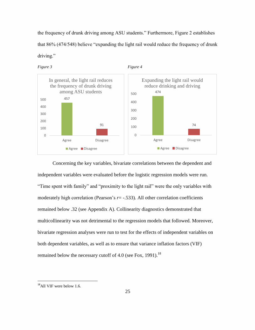
the frequency of drunk driving among ASU students.” Furthermore, Figure 2 establishes

that 86% (474/548) believe “expanding the light rail would reduce the frequency of drunk

driving.”

Figure 3 Figure 4

Concerning the key variables, bivariate correlations between the dependent and

independent variables were evaluated before the logistic regression models were run.

“Time spent with family” and “proximity to the light rail” were the only variables with

moderately high correlation (Pearson’s r= -.533). All other correlation coefficients

remained below .32 (see Appendix A). Collinearity diagnostics demonstrated that

multicollinearity was not detrimental to the regression models that followed. Moreover,

bivariate regression analyses were run to test for the effects of independent variables on

both dependent variables, as well as to ensure that variance inflation factors (VIF)

remained below the necessary cutoff of 4.0 (see Fox, 1991).18

18

All VIF were below 1.6.

457

91

0

100

200

300

400

500

Agree Disagree

In general, the light rail reduces

the frequency of drunk driving

among ASU students

Agree Disagree

474

74

0

100

200

300

400

500

Agree Disagree

Expanding the light rail would

reduce drinking and driving

Agree Disagree

26

Table 2.

Binge Drinking Negative Binomial Regression Model.

b SE Exp(b)

Live within walking

distance of the LR .559*** .159 3.52

Frequency of use of the LR -.080 .044 -1.83

Self-control (mean score) -.969*** .141 -6.85

Peers drink and drive .478*** .110 4.34

Age .002 .014 .11

Male .242 .127 1.9

Non White .074 .134 .56

Credit hours -.448** .171 -2.61

Time spent with family -.232*** .042 -5.42

Employed .242 .135 1.79

Driver .747** .239 3.13

Constant 3.295*** .714 4.61

McFadden’s R2=.072

Note: Entries are unstandardized coefficients (b).

*p< .05. ** p< .01. ***p<.001 (two-tailed test)

Now turning the attention to the first research question, to what extent is binge

drinking predicted by proximity to the light rail and frequency of its use? Table 2

presents the negative binomial model predicting binge drinking, which shows significant

test of fit and a McFadden’s R square value of .072. The model demonstrates that living

within a reasonable walking distance is statistically significant in predicting binge

drinking (b= .559 p< .001). The incident rate ratio in this instance demonstrates that for

individuals who live closer to the light rail there exists a 75% increase in the number of

occasions an individual reports binge drinking (1.75= 1-[exp.(.559)]). However,

frequency of use of the light rail was not found to be associated with binge drinking.

Additionally, as expected, self-control and peer delinquency also had statistically

significant relationships with binge drinking in the expected direction. Specifically, high

27

self-control was inversely related to self-reported binge drinking. Having delinquent

peers increased the likelihood of binge drinking by about 61%. Finally, the routine

activities measures time spent with family and amount of credit hours taken, also

revealed a significant inverse relationship with binge drinking. It is notable that the

inconsistency in the results between the two light rail measures is surprising. Two

possible explanations will be elaborated on in the discussion section.

Table 3.

Drinking and Driving Logistic Regression Model.

b SE Exp(b)

live within walking

distance of LR -.567 .353 .567

Frequency of LR use -.252* .108 .777

Self-control (mean

score) -1.439*** .304 .237

Peers drink and drive 1.248*** .231 3.485

Age .007 .030 1.007

Gender (1= male) .703* .285 2.019

Race (Non White= 1) .413 .291 1.512

Credit hours .190 .212 1.210

Time spent with family -.047 .096 .954

Employed -.067 .300 .935

Driver .740 .780 2.096

Constant -.258 1.542 .772

Nagelkerke’s R2=.299

Note: Entries are unstandardized coefficients (b).

*p< .05. ** p< .01. ***p<.001 (two-tailed test)

Table 3 displays the logistic regression model predicting drunk driving, one of the

central investigations in the thesis. The model test of fit is significant with a Negelkerke’s

R square value of .29 which is moderate in size. Frequency of use of the light rail is

found to be statistically significant and associated with a 23% decline in the odds of

drunk driving (1/.77=.298). The item measuring residential proximity to the light rail did

28

not fare as well. Interestingly the self-control and social learning variables remain

statistically significant in this model as well. The logistic regression coefficients indicate

that higher self-control scores are related to a reduced likelihood of drunk driving.

Conversely, having peers that drink and drive triples the odds that a respondent will also

report drunk driving. In terms of demographic variables, males are twice as likely as

females to report during under the influence of alcohol. No other control variables are

significant.

DISCUSSION

With temperatures that routinely exceed 110° Fahrenheit during the summer, the

Phoenix metropolitan area is decidedly governed by the heat. While other cities grew in

size and population, those cities’ civil engineers were able to keep up with evolving

transportation concerns (Smith, 1984). As Phoenix’s population began to grow outward,

however, the heat and sprawl of the city likely caused extensive public transportation

systems to take a back seat to the comfort of personally owned vehicles (Arizona

Department of Administration, 2011; Kuby, et al, 2004). The trolley carbarn fire of 1947

was an additional nail in the coffin for any Phoenician’s hopes of an affordable network

of buses and railcars (Fleming, 1977). In 2008, when the Valley Metro light rail became

operational, the new railcars were entering a more complex city environment compared

to what the previous railcar system left behind. Large university campuses now populate

the metropolitan landscape, in addition to extensive entertainment venues, and dense

clusters of bars and restaurants. Statistically speaking, due to the fact college students are

not strangers to drinking or driving under the influence of alcohol (Nagin & Paternoster,

29

1993; Cohen, 1990), the current study attempted to investigate if their behavioral patterns

would be affected by the re-implemented rail system.

Respondents in the current study acknowledged, perhaps in more ways than one,

that the Phoenix metro light rail is a factor in their decision making processes relating to

binge drinking and driving impaired. Living reasonably close to the light rail was found

to be positively associated with binge drinking. Two possible explanations exist for this

association. First, it is possible that students who live near the light rail are likely to feel

fewer inhibitions with that fact in mind when they go out to socialize and drink alcohol,

thereby affecting their amount of alcohol consumption. Second, the light rail runs near

two large college campuses. It is possible that students who live within reasonable

walking distance of the light rail also live on or near campus. This would mean that a

respondent’s distance to campus may be associated to their likelihood of participating in

college drinking games and activities. It is noteworthy, however, that ASU is a dry

campus and alcohol is forbidden in the dormitories (though likely still subsists there).

Further research is needed to determine which possibility is more likely, but both suggest

interesting findings in terms of student behavior.

If it is the case the students are choosing to drink to excess because they know

they have an easily accessible light rail ride home, this may still have positive

implications. While binge drinking is not necessarily a positive outcome from a policy

standpoint, in this instance it may be the lesser of two evils. A student who decides to

drink to excess, but elects not to drive home, is less of a public health risk than a student

who has one too many and gets behind the wheel of a car. The net impact of damage

30

resulting from drunk driver is arguably greater than the public disorder and ordinance

violations resulting from students stumbling to the light rail in a drunken state.

Furthermore, an intoxicated individual on the light rail may prove to be a more difficult

target to victimize due to the fact that the light rail is well lit and has electronic security

and police officers patrolling its cars.

The more promising finding of this study is that those who report riding the light

rail more report less drinking and driving. This suggests that a cultural shift in positive

views of public transportation as a result of the light rail may pay long term dividends in

terms of public health and city planning. This point is more salient with the fact that

follow-up models specified with the same predictors estimating use of city buses were

not associated with binge drinking or drunk driving. This provides some credibility to the

claim that the light rail is more reliable and perhaps easier to use by students while

intoxicated than the city bus system. The current findings further demonstrate the need

for research on public transportation and its effects on driving under the influence.

Further, these findings illustrate a number of policy implications. One implication is that

it may be a smart investment for city planners to think about making the light rail system

more attractive for the 70,000 students at ASU, removing the obstacles to optimizing its

use, and better publicizing its availability. The light rail averages 15 minute wait times

between cars, and each car only travels an average of 22 miles an hour (Valley Metro,

2013). Increasing the number of light rail cars and removing additional roadway

impediments to rail cars completing travel routes faster might increase ridership among

students who might not use the system for lack of patience (incidentally a measure of low

31

self-control). Also, civil engineers may come to discover that extending the amount of

rail service during certain evenings, and for particular rail car routes may have provide

additional public health benefits. As evidence, 36.3% of the study sample indicated that if

the light rail went to at least one of four entertainment districts they would be less likely

to drive drunk. Furthermore, providing an incentive for establishments that serve alcohol

to build closer to public transportation lines may also assist in reducing drunk driving and

public disorder offenses.

On a broader scale, however, this study highlights the need for more extensive

research to be performed with regard to providing safer travel options for university

populations especially within the realm of public transportation. The public should be

provided public service reminders that alternatives to drinking and driving exist, and

perhaps this awareness should be prompted with signage and pamphlets in an around

popular socializing venues at ASU. Additionally, if it is the case that there will be an

increase in the population of inebriated individuals using public transportation, special

security considerations should also be considered –since there will be an increase in

individuals who are more easily victimized. Furthermore, additional research is required

to determine if individuals are specifically using the light rail to and from their homes

and drinking locations in order to avoid driving drunk. Geospatial analyses may be the

most definitive method in determining this relationship. Additional analyses should also

determine if a significant interaction effect exists between light rail use and self-control.

In other words are people with low self-control specifically more likely to use the light

rail (especially when inebriated) or are the effects general across the population.

32

Finally, this research sheds more light on the fact that deterrence through

sanctions and increased enforcement does not have to be the only way to prevent people

from driving drunk. Altering routine activities through thoughtful city planning and

entrepreneurial activities can be effective in restructuring activity patterns and controlling

crime. These situational measures should be considered in addition to deterrence based

policies if a municipality intends to give its young citizens an opportunity structure that

leads to the avoidance of crime.

33

REFERENCES

Adebayo, A., (1988) Drunk Driving Intervention in an Urban Community: an

Exploratory Analysis. The British Journal of Addiction. 83. 423-429.

Applegate, B., Cullen, F., Link, B., Richards, P., Lanza-Kaduce, L., (1996) Determinants

of Public Punitiveness Toward Drunk Driving; A Factorial Survey Approach.

Justice Quarterly. 13. 57-80.

Arizona Department of Administration. (2011) "Population Estimate for July 1, 2011."

Phoenix, Arizona.

http://phoenix.gov/webcms/groups/internet/@inter/@dept/@dsd/

documents/web _content/pdd_pz_pdf_00178.pdf

Arizona Revised Statutes (2007) Title 28; Driving Under the Influence: 28-1381.1.

Arizona State University (2010). ASU Enrollment Data

http://diversity.asu.edu/asu-diversity

Arizona State University (2012). Parking and Transit Services

https://cfo.asu.edu/pts-transit-pass

Baron, E. and Dickerson, M. (1999) Alcohol Consumption and Self-Control of Gambling

Behaviour. Journal of Gambling Studies. 15. 3-15.

Baumeister, R. (2002) Ego Depletion and Self-Control Failure: An Energy Model of the

Self’s Executive Function. Self and Identity. 1. 129-136.

Baumeister, R., Heatherton, T. (1996) Self-Regulation Failure: An Overview.

Psychological Inquiry. 7. 1-15.

34

Carpenter, C. (2004). How Do Zero Tolerance Laws Work? Journal of Health

Economics. 23. 61-83.

Clarke, R. (1995). Situational Crime Prevention. Crime and Justice. 19. 91-150

Cohen, R. (1992).Drunk Driving. Office of Justice Programs, Bureau of Justice Statistics,

U.S. Department of Justice

Cohen, L., & Felson, M. (1979). Social change and crime rate trends: A routine activity

approach. American Sociological Review. 44.4. 588-608.

DiBlasio, F. (1986). Drinking Adolescents on the Roads. Journal of Youth and

Adolescents. 15, 2. 173-188.

DiBlasio, F. (1987). Predriving riders and drinking riders. Journal of Alcohol. 49, 1. 11-

15.

Durkin, K., Wolfe, T., Clark, G. (1999) Social Bond Theory and Binge Drinking Among

College Students: A Multivariate Analysis. College Student Journal. 33. 450-462.

Felson, M., Cohen, L. (1980) Human Ecology and Crime: A Routine Activity Approach.

Human Ecology. 8. 389-406.

Fisher, B., Sloan, J., Cullen, F., Lu, C. (1998) Crime in the Ivory Tower: The Level and

Sources of Student Victimization. Criminology. 36. 671-709.

Fillmore, M., Vogel-Sprott, M. (1999) An Alcohol Model of Impaired Inhibitory Control

and Its Treatment in Humans. Experimental and Clinical Psychopharmacology. 7.

49-55.

Fleming, L. (1977) Ride a Mile Smile the While. Phoenix, Az. Swaine publications, Inc.

Fox, J. (1991). Regression diagnostics. Newbury Park, CA: Sage.

35

Gibson, C., Schrek, C., & Miller, M. (2004) Binge Drinking and Negative Alcohol-

Related Behaviors: A Test of Self-control Theory. Journal of Criminal Justice.

32. 411-420.

Gottfredson, M., and Hirschi, T. (1990). A General Theory of Crime. Palo Alto, CA:

Stanford University Press.

Grohosky, A., Moore, K. & Ochshorn, E. (2007) An Alcohol Policy Evaluation of

Drinking and Driving in Hillsborough County, Florida. Criminal Justice Policy

Review. 18. 434-450.

Gruenewald, P., Mitchell, P., & Treno, A. (1996) Drinking and Driving: Drinking

Patterns and Drinking Problems. Addiction. 1637-1649.

Gruenewald, P., Johnson, F., & Treno, A. (2002) Outlets, Drinking and Driving: A

Multilevel Analysis of Availability. Journal of Studies on Alcohol. 63. 460-477.

Helander, C. (2002). DUI Countermeasures in California: What Works and What

Doesn’t, With Recommendations for Legislative Reform. Report to the

Legislature of the State of California.

Holtfreter, K., Reisig, M., Pratt, T. (2008) Low Self-Control, Routine activities and Fraud

Victimization. Criminology. 46. 189-220.

Jackson, C., Owens, E. (2011) One for the Road: Public Transportation, Alcohol

Consumption, and Intoxicated Driving. Journal of Public Economics. 95. 106-

121.

36

Joshi, H., Guhathakurta, S., Konjevod, G., Crittenden, J., Li, K. (2006) Simulating the

Effect of Light Rail on Urban Growth in Phoenix: An Application of the

UrbanSim Modeling Environment. Journal of Urban Technology. 13. 91-111.

Keane, C., Maxim, P., and Teevan, J. (1993) Drinking and Driving, Self-control, and

Gender: Testing a General Theory of Crime. Journal of Research in Crime. 30.

30-46

Kingsnorth, R. (1993). Specific Deterrence and the DUI Offender: The Impact of

California’s Administrative Per Se Law. The Journal of Contemporary Criminal

Justice, 9, 328-342.

Kuby, M., Barranda, A., & Upchurch, C. (2004) Factors Influencing Light-rail Station

Boardings in the United States. Transportation Research Part A. 38. 223-247.

Lanza-Kaduce, L. (1988) Perceptual Deterrence and Drinking and Driving among

College Students. Criminology. 26. 331-341.

Lauritsen, J., Sampson, R., & Laub, J., (1991) The Link Between Offending and

Victimization Among Adolescents. Criminology. 29. 265-292.

McCartt, A., Hellinga, L., &Wells, J. (2008) Effects of a College Community Campaign

on Drinking and Driving With a Strong Enforcement Component. Insurance

Institute for Highway Safety. From: Young Impaired Drivers: The Nature of the

Problem and Possible Solutions

Muraven, M., Collins, R., & Nienhaus, K. (2002) Self-Control and Alcohol Restraint: An

Initial Application of the Self-Control Strength Model. Psychology of Addictive

Behaviors. 16. 113-120.

37

Muraven, M., Pogarsky, G., & Shmueli, D. (2006) Self-control Depletion and the General

Theory of Crime. Journal of Quantitative Criminology.22.223-267.

Nagin, D., Paternoster, R. (1993) Enduring Individual Differences and Rational Choice

Theories of Crime. Law and Society Review. 27. 467-496.

National Highway Traffic and Safety Administration (2010). Highlights of Motor

Vehicle Crashes, Traffic Safety Facts, Retrieved from

http://www-nrd.nhtsa.dot.gov/Pubs/811363.pdf

Náñez, D. (2008) Tempe Begins Light-rail Service with Parties, Az Central

http://www.azcentral.com/news/traffic/lightrail/articles/2008/12/01/20081201tr

lightrailtalk1129.html

O’Donnell, M. (1985). Research on Drinking Locations of Alcohol-Impaired Drivers:

Implications for Prevention Policies. Journal of Public Health Policy, 6, 510-525.

Ornstein, S., Hanssens, D. (1985).Alcohol Control Laws and the Consumption of

Distilled Spirits and Beer. Journal of Consumer Research, 12, 200-213.

Piquero, A., & Tibbetts, S. (1996) Specifying the Direct and Indirect Effects of Low Self

Control and Situation Factors In Offenders’ Decision Making: Toward a More

Complete Model of Rational Decision Making. Justice Quarterly. 13. 481-510.

Piquero, A., Gibson, C., & Tibbetts, S. (2002) Does Self-control Account for the

Relationship Between Binge-drinking and Alcohol Related Behaviors. Criminal

Behavior and Mental Health. 12. 135-154.

Pratt, T., & Cullen, F. (2000) The Empirical Status of Gottfredson and Hirschi’s General

Theory of Crime: A Meta-Analysis. Criminology. 38. 931-964.

38

Pratt, T., & Cullen, F. (2005) Assessing Macro-Level Predictors and Theories of Crime: A

Meta-Analysis. Michael Tonry (Ed.), Crime and Justice: A Review of Research. 32.

p. 373-450.

Pratt, T., Cullen, F., Blevins, K., Daigle, L., & Madensen, T. (2008) The Empirical Status

of Deterrence Theory: A Meta- Analysis (eds.) Taking Stock: The Status of

Criminological Theory. Advances in Criminological Theory. Vol 15. New

Brunswick, NJ: Transaction.

Pratt, T., & Reisig, M. (2011). Low Self-Control and Imprudent Behaviors Revisted.

Deviant Behavior. 32: 589–625

Raub, R., Lucke, R., & Warke, R. (2003) Breath Alcohol Ignition Interlock Devices:

Controlling the Recidivist. Traffic Injury Prevention. 4. 199-205.

Robertson, R., & Marples, I. (2008) Alcohol Monitoring Technologies: Applications for

Youth and Young Impaired Drivers. Transportation Research Board.

Ross, H. L., & Gonzales, P. (1988) The Effects of License Revocation on Drunk-driving

Offenders. Accident Analysis and Prevention. 20. 379- 391.

Schell, T., Chan, K., & Morral, A. (2006) Predicting DUI recidivism: Personality,

Attitudinal, and Behavioral Risk Factors. Drug and Alcohol Dependence. 82. 33-

40.

Sherman, L., Gartin, P., & Buerger, M. (1989) Hot Spots of Predatory Crime: Routine

Activities and the Criminology of Place. Criminology. 27. 27-55.

39

Shore, E., & Maguin, E. (1988) Deterrence of Drinking-Driving: The Effect of Changes

in the Kansas Driving Under the Influence Law. Evaluation and Program

Planning. 11. 245- 254.

Shults, R., Elder, R., Sleet, D., Nichols, J., Alao, M., Carande-Kuli, V., Zaza, S.,

Sosin, D., Thompson, R. (2001) Task Force on Community Preventive Services.

Reviews of evidence regarding interventions to reduce alcohol-impaired driving.

American Journal of Preventive Medicine.21, 66-88.

Smith, W. (1984). Mass Transport for High-Rise High-Density Living. Journal of

Transportation Engineering. 110, 6. 521-535.

Stewart, K. (2008) Young Impaired Drivers: The Nature of the Problem and Possible

Solutions: Overview. Transportation Research Board.

Tangney, J., Baumeister, R., & Boone, A. (2008) High Self-Control Predicts Good

Adjustment, Less Pathology, Better Grades, and Interpersonal Success. Journal of

Personality 72: 271–324.

Tibbetts, S. & Myers, D. (1999) Low Self-control, Rational Choice, and Student Test

Cheating. American Journal of Criminal Justice. 23, 179-200

Timmerman, M., Geller, E., Glindemann, K., Fournier, A. (2003) Do the Designated

Drivers of College Students Stay Sober. Journal of Safety Research. 34, 127-133.

Valley Metro (2013). Transit Maps. Retrieved from:

http://www.valleymetro.org/down_loads/maps/

40

Valley Metro (2013). Fast Facts. Retrieved from:

http://www.valleymetro.org/images/uploads/lightrail_publications/

Fast_Facts_Oct2013.pdf

Wechsler, H. (1997). Harvard College Alcohol Survey: Codebook. Inter-University

Consortium for Political and Social Research. 1-196.

Wechsler, H., Dowdall, G.W., Davenport, A., & Castillo, S. (1995). Correlates of College

Student Binge Drinking. American Journal of Public Health. 85, 7, 921-926.

Wiliszowski, C., Murphy, P., Jones, R., & Lacey, J (1996) Determine the Reasons for

Repeat Drinking and Driving. Mid-America Research Institute. Winchester, MA.

Wright, B., Caspi, A., Moffitt, T., & Paternoster, R. (2004) Does Perceived Risk of

Punishment Deter Criminally Prone Individuals? Rational Choice, Self-control

and Crime. Journal of Research in Crime and Delinquency. 41. 180-213.

Wooster, M., (2000). Mothers Against Drunk Driving: Has Its Vision Become Blurred.

Alternatives in Philanthropy, 1-6.

Zhang, L., Wieczorek, W.,& Welte, J. (1997). The Nexus between Alcohol and Violent

Crime Alcoholism: Clinical and Experimental Research. 21. 1264-1271.

APPENDIX A

CORRELATION MATRIX

Ap

pen

dix

A. P

ears

on

’s r

Co

rrela

tio

n C

oeff

icie

nts

Vari

ab

les

Y1

Y2

X1

X2

X3

X4

X5

X6

X7

X8

X9

X10

X11

X12

Y1

Dra

nk a

nd

dro

ve

1

Y2

Bin

ge d

rin

ker

.260*

*1

X1

Pro

xim

ity

to

LR

-.092*

.161*

*1

X2

Fre

qu

en

cy

of

LR

use

-.146*

*-0

.079

0.0

76

1

X3

Self

-co

ntr

ol

-.246*

*-.

303*

*-.

114*

*0.0

41

1

X4

Fre

qu

en

cy

of

frie

nd

s

dru

nk d

riv

ing

.316*

*.1

82*

*-.

098*

-0.0

81

-.179*

*1

X5

Ag

e0.0

27

-0.0

39

-.210*

*0.0

56

0.0

44

0.0

24

1

X6

Male

0.0

09

-.271*

*0.0

30.0

12

-0.0

27

0.0

16

0.0

52

1

X7

Race

0.0

78

0.0

16

-.129*

*-0

.001

.088*

.127*

*0.0

55

-0.0

71

1

X8

Cre

dit

ho

urs

-0.0

49

-0.0

53

.263*

*-0

.013

0.0

31

-.084*

-.307*

*0.0

54

-0.0

66

1

X9

Em

plo

yed

0.0

15

0.0

52

-.170*

*-0

.081

0.0

43

.130*

*0.0

06

0.0

26

0.0

48

-0.0

79

1

X10

Fam

ily

tim

e0.0

26

-.174*

*-.

533*

*-0

.049

.128*

*0.0

43

.155*

*-0

.003

.173*

*-.

155*

*.0

93*

1

X11

Dri

ver

.085*

0.0

45

-.237*

*-.

113*

*0.0

24

.163*

*0.0

54

0.0

43

0.0

28

-.085*

.131*

*.2

10*

*1

X12

Dri

nker

.167*

*0.0

62

0.0

38

0.0

35

-0.0

71

0.0

67

-.169*

*-0

.038

-0.0

45

0.0

78

0.0

60.0

39

-0.0

11

APPENDIX B

BINGE DRINKING LOGISTIC REGRESSION MODEL

Binge Drinking Logistic Regression Model.

b SE Exp(b)

Live within walking

distance of the LR .573* .240 1.773

Frequency of use of the LR -.083 .067 .920

Self-control (mean score) -1.190*** .214 .304

Peers drink and drive .451** .157 1.570

Age -.007 .020 .993

Male .296 .193 1.345

Non White .296 .199 1.345

Credit hours -.200 .147 .819

Time spent with family -.175** .067 .839

Employed .379 .206 1.462

Driver .509 .347 1.664

Constant 2.752** .998 15.670

Nagelkerke’s R2=.210

Note: Entries are unstandardized coefficients (b).

*p< .05. ** p< .01. ***p<.001 (two-tailed test)