Drilling Technology and Costs - Geothermal · PDF fileChapter 6 Drilling Technology and Costs...
51
CHAPTER 6 Drilling Technology and Costs 6.1 Scope and Approach _ _ _ _ _ _ _ _ _ _ _ _ _ _ _ _ _ _ _ _ _ _ _ _ _ _ _ _ _ _ _ _ _ _63 6.2 Review of Geothermal Drilling Technology _ _ _ _ _ _ _ _ _ _ _ _ _ _ _ _ _ _ _ _64 6.2.1 Early geothermal/EGS drilling development _ _ _ _ _ _ _ _ _ _ _ _ _ _ _ _ _ _ _64 6.2.2 Current EGS drilling technology _ _ _ _ _ _ _ _ _ _ _ _ _ _ _ _ _ _ _ _ _ _ _ _ _ _65 6.3 Historical WellCost Data _ _ _ _ _ _ _ _ _ _ _ _ _ _ _ _ _ _ _ _ _ _ _ _ _ _ _ _ _ _ _68 6.3.1 General trends in oil and gas wellcompletion costs _ _ _ _ _ _ _ _ _ _ _ _ _ _69 6.3.2 MIT Depth Dependent (MITDD) drillingcost index _ _ _ _ _ _ _ _ _ _ _ _ _ _ _612 6.3.3 Updated geothermal well costs _ _ _ _ _ _ _ _ _ _ _ _ _ _ _ _ _ _ _ _ _ _ _ _ _617 6.4 Predicting Geothermal Well Costs with the Wellcost Lite Model _ _ _ _ _ _618 6.4.1 History of the Wellcost Lite model _ _ _ _ _ _ _ _ _ _ _ _ _ _ _ _ _ _ _ _ _ _ _ _618 6.4.2 Wellcost Lite model description _ _ _ _ _ _ _ _ _ _ _ _ _ _ _ _ _ _ _ _ _ _ _ _ _619 6.5 DrillingCost Model Validation _ _ _ _ _ _ _ _ _ _ _ _ _ _ _ _ _ _ _ _ _ _ _ _ _ _ _619 6.5.1 Basecase geothermal wells _ _ _ _ _ _ _ _ _ _ _ _ _ _ _ _ _ _ _ _ _ _ _ _ _ _ _619 6.5.2 Comparison with geothermal wells _ _ _ _ _ _ _ _ _ _ _ _ _ _ _ _ _ _ _ _ _ _ _622 6.5.3 Comparison with oil and gas wells _ _ _ _ _ _ _ _ _ _ _ _ _ _ _ _ _ _ _ _ _ _ _622 61 6.5.4 Model input parameter sensitivities and drillingcost breakdown _ _ _ _ _ _ _623 6.6 Emerging Drilling Technologies _ _ _ _ _ _ _ _ _ _ _ _ _ _ _ _ _ _ _ _ _ _ _ _ _ _627 6.6.1 Current oil and gas drilling technologies adaptable to EGS _ _ _ _ _ _ _ _ _ _627 6.6.2 Revolutionary drilling technologies _ _ _ _ _ _ _ _ _ _ _ _ _ _ _ _ _ _ _ _ _ _ _628 6.7 Conclusions _ _ _ _ _ _ _ _ _ _ _ _ _ _ _ _ _ _ _ _ _ _ _ _ _ _ _ _ _ _ _ _ _ _ _ _ _ _ _629 References _ _ _ _ _ _ _ _ _ _ _ _ _ _ _ _ _ _ _ _ _ _ _ _ _ _ _ _ _ _ _ _ _ _ _ _ _ _ _ _ _ _ _631 Appendices _ _ _ _ _ _ _ _ _ _ _ _ _ _ _ _ _ _ _ _ _ _ _ _ _ _ _ _ _ _ _ _ _ _ _ _ _ _ _ _ _ _ _633 A.6.1 WellCost Data _ _ _ _ _ _ _ _ _ _ _ _ _ _ _ _ _ _ _ _ _ _ _ _ _ _ _ _ _ _ _ _ _ _ _ _ _ _633 A.6.2 Wellcost Lite Model _ _ _ _ _ _ _ _ _ _ _ _ _ _ _ _ _ _ _ _ _ _ _ _ _ _ _ _ _ _ _ _ _ _ _ _637 A.6.2.1 Background and brief history of the development of Wellcost Lite _ _ _ _ _ _637 A.6.2.2 Wellcost Lite – How does the cost model work? _ _ _ _ _ _ _ _ _ _ _ _ _ _ _ _637 A.6.3 Model Results for Specific Areas and Depths _ _ _ _ _ _ _ _ _ _ _ _ _ _ _ _ _ _ _ _ _ _649 A.6.4 Model Results for Reworked Wells _ _ _ _ _ _ _ _ _ _ _ _ _ _ _ _ _ _ _ _ _ _ _ _ _ _ _651 A.6.4.1 Rig on drilling/deepening 460 m (1,500 ft)/rig still on the well _ _ _ _ _ _ _ _651 A.6.4.2 Rig on drilling/sidetracked lateral/as a planned part of the well design _ _ _651 A.6.4.3 Reworks/rig has to be mobilized/add a lateral for production maintenance/a workover _ _ _ _ _ _ _ _ _ _ _ _ _ _ _ _ _ _ _ _ _ _651 A.6.4.4 Redrills to enhance production/a workover/rig to be mobilized _ _ _ _ _ _ _651
Transcript of Drilling Technology and Costs - Geothermal · PDF fileChapter 6 Drilling Technology and Costs...

C H A P T E R 6
Drilling Technology and Costs 6.1 Scope and Approach _ _ _ _ _ _ _ _ _ _ _ _ _ _ _ _ _ _ _ _ _ _ _ _ _ _ _ _ _ _ _ _ _ _63
6.2 Review of Geothermal Drilling Technology _ _ _ _ _ _ _ _ _ _ _ _ _ _ _ _ _ _ _ _64
6.2.1 Early geothermal/EGS drilling development _ _ _ _ _ _ _ _ _ _ _ _ _ _ _ _ _ _ _64
6.2.2 Current EGS drilling technology _ _ _ _ _ _ _ _ _ _ _ _ _ _ _ _ _ _ _ _ _ _ _ _ _ _65
6.3 Historical WellCost Data _ _ _ _ _ _ _ _ _ _ _ _ _ _ _ _ _ _ _ _ _ _ _ _ _ _ _ _ _ _ _68
6.3.1 General trends in oil and gas wellcompletion costs _ _ _ _ _ _ _ _ _ _ _ _ _ _69
6.3.2 MIT Depth Dependent (MITDD) drillingcost index _ _ _ _ _ _ _ _ _ _ _ _ _ _ _612
6.3.3 Updated geothermal well costs _ _ _ _ _ _ _ _ _ _ _ _ _ _ _ _ _ _ _ _ _ _ _ _ _617
6.4 Predicting Geothermal Well Costs with the Wellcost Lite Model _ _ _ _ _ _618
6.4.1 History of the Wellcost Lite model _ _ _ _ _ _ _ _ _ _ _ _ _ _ _ _ _ _ _ _ _ _ _ _618
6.4.2 Wellcost Lite model description _ _ _ _ _ _ _ _ _ _ _ _ _ _ _ _ _ _ _ _ _ _ _ _ _619
6.5 DrillingCost Model Validation _ _ _ _ _ _ _ _ _ _ _ _ _ _ _ _ _ _ _ _ _ _ _ _ _ _ _619
6.5.1 Basecase geothermal wells _ _ _ _ _ _ _ _ _ _ _ _ _ _ _ _ _ _ _ _ _ _ _ _ _ _ _619
6.5.2 Comparison with geothermal wells _ _ _ _ _ _ _ _ _ _ _ _ _ _ _ _ _ _ _ _ _ _ _622
6.5.3 Comparison with oil and gas wells _ _ _ _ _ _ _ _ _ _ _ _ _ _ _ _ _ _ _ _ _ _ _622 61
6.5.4 Model input parameter sensitivities and drillingcost breakdown _ _ _ _ _ _ _623
6.6 Emerging Drilling Technologies _ _ _ _ _ _ _ _ _ _ _ _ _ _ _ _ _ _ _ _ _ _ _ _ _ _627
6.6.1 Current oil and gas drilling technologies adaptable to EGS _ _ _ _ _ _ _ _ _ _627
6.6.2 Revolutionary drilling technologies _ _ _ _ _ _ _ _ _ _ _ _ _ _ _ _ _ _ _ _ _ _ _628
6.7 Conclusions _ _ _ _ _ _ _ _ _ _ _ _ _ _ _ _ _ _ _ _ _ _ _ _ _ _ _ _ _ _ _ _ _ _ _ _ _ _ _629
References _ _ _ _ _ _ _ _ _ _ _ _ _ _ _ _ _ _ _ _ _ _ _ _ _ _ _ _ _ _ _ _ _ _ _ _ _ _ _ _ _ _ _631
Appendices _ _ _ _ _ _ _ _ _ _ _ _ _ _ _ _ _ _ _ _ _ _ _ _ _ _ _ _ _ _ _ _ _ _ _ _ _ _ _ _ _ _ _633
A.6.1 WellCost Data _ _ _ _ _ _ _ _ _ _ _ _ _ _ _ _ _ _ _ _ _ _ _ _ _ _ _ _ _ _ _ _ _ _ _ _ _ _633
A.6.2 Wellcost Lite Model _ _ _ _ _ _ _ _ _ _ _ _ _ _ _ _ _ _ _ _ _ _ _ _ _ _ _ _ _ _ _ _ _ _ _ _637
A.6.2.1 Background and brief history of the development of Wellcost Lite _ _ _ _ _ _637
A.6.2.2 Wellcost Lite – How does the cost model work? _ _ _ _ _ _ _ _ _ _ _ _ _ _ _ _637
A.6.3 Model Results for Specific Areas and Depths _ _ _ _ _ _ _ _ _ _ _ _ _ _ _ _ _ _ _ _ _ _649
A.6.4 Model Results for Reworked Wells _ _ _ _ _ _ _ _ _ _ _ _ _ _ _ _ _ _ _ _ _ _ _ _ _ _ _651
A.6.4.1 Rig on drilling/deepening 460 m (1,500 ft)/rig still on the well _ _ _ _ _ _ _ _651
A.6.4.2 Rig on drilling/sidetracked lateral/as a planned part of the well design _ _ _651
A.6.4.3 Reworks/rig has to be mobilized/add a lateral for production maintenance/a workover _ _ _ _ _ _ _ _ _ _ _ _ _ _ _ _ _ _ _ _ _ _651
A.6.4.4 Redrills to enhance production/a workover/rig to be mobilized _ _ _ _ _ _ _651

Chapter 6 Drilling Technology and Costs
6.1 Scope and Approach Exploration, production, and injection well drilling are major cost components of any geothermal project (Petty et al., 1992; Pierce and Livesay, 1994; Pierce and Livesay, 1993a; Pierce and Livesay, 1993b). Even for highgrade resources, they can account for 30% of the total capital investment; and with lowgrade resources, the percentage increases to 60% or more of the total. Economic forecasting of thermal energy recovery by Enhanced Geothermal System (EGS) technologies requires reliable estimates of well drilling and completion costs. For this assessment, a cost model – flexible enough to accommodate variations in welldesign parameters such as depth, production diameter, drilling angle, etc. – is needed to estimate drilling costs of EGS wells for depths up to 10,000 m (32,800 ft).
Although existing geothermal wellcost data provide guidance useful in predicting these costs, there are insufficient numbers of geothermal well records, of any kind, to supply the kind of parametric variation needed for accurate analysis. Currently, there are fewer than 100 geothermal wells drilled per year in the United States, few or none of which are deep enough to be of interest. Very few geothermal wells in the United States are deeper than 2,750 m (9,000 ft), making predictions of deep EGS wells especially difficult. Although there are clear differences between drilling geothermal and oil and gas wells, many insights can be gained by examining technology and cost trends from the extensive oil and gas well drilling experience.
Thousands of oil/gas wells are drilled each year in the United States, and data on the well costs are readily available (American Petroleum Institute, JAS, 19762004). Because the process of drilling oil and gas wells is very similar to drilling geothermal wells, it can be assumed that trends in the oil and gas industry also will apply to geothermal wells. Additionally, the similarity between oil and gas wells and geothermal wells makes it possible to develop a drilling cost index that can be used to normalize the sparse data on geothermal well costs from the past three decades to current currency values, so that the wells can be compared on a common dollar basis. Oil and gas trends can then be combined with existing geothermal well costs to make rough estimates of EGS drilling costs as a function of depth.
Oil and gas well completion costs were studied to determine general trends in drilling costs. These trends were used to analyze and update historical geothermal well costs. The historical data were used to validate a drilling cost model called Wellcost Lite, developed by Bill Livesay and coworkers. The model estimates the cost of a well of a specific depth, casing design, diameter, and geological environment. A series of basecase geothermal well designs was generated using the model, and costs for these wells were compared to costs for both existing geothermal wells and oil and gas wells over a range of depths. Knowledge of the specific components of drilling costs was also used to determine how emerging and revolutionary technologies would impact geothermal drilling costs in the future.
63

Chapter 6 Drilling Technology and Costs
6.2 Review of Geothermal Drilling Technology6.2.1 Early geothermal/EGS drilling development The technology of U.S. geothermal drilling evolved from its beginning in the early 1970s with a flurry of activity in The Geysers field – a vapordominated steam field – in Northern California. Although international geothermal development began before the 1960s in places such as Italy at Lardarello, New Zealand, and Iceland, the development of The Geysers field in northern California was the first big U.S project. Problems encountered during drilling at The Geysers, such as fractured hard and abrasive formations, extreme lost circulation, and the higher temperatures were overcome by adaptation and innovation of existing oil and gas technology to the demanding downhole environment in geothermal wells. The drilling at The Geysers resulted in the reconfiguration of rigs specially outfitted for drilling in that environment.
These early geothermal wells at The Geysers were perceived to lie in a category somewhere between “deep, hot, water wells” and “shallow oil/gas wells.” Later, other U.S. geothermal drilling activities started in the hydrothermal environments of Imperial Valley in California, the Coso field in East Central California, and Dixie Valley in Northern Nevada. Imperial Valley has a “layercake” arrangement of formations, very similar to a sedimentary oil and gas field. Here, geothermal fluids are produced in the boundaries of an area that has subsided due to the action of a major fault (San Andreas). The Salton Sea reservoir is in the Imperial Valley about 25 miles from El Centro, California. Some extremely productive wells have been drilled and are producing today at this site, including Vonderahe 1, which is the most productive well in the continental United States. An extension of the same type of resource crosses over into Northern Mexico near Cierro Prieto. Approximately 300 MWe are generated from the Salton Sea
64 reservoir and more than 720 MWe from Ciero Prieto. Northern Nevada has numerous power producing fields. Dixie Valley is a relatively deep field (> 3,000 m or 9,000 ft) near a fault line.
In parallel with these U.S. efforts, geothermal developments in the Philippines and Indonesia spurred on the supply and service industries. There was continual feedback from these overseas operations, because, in many cases, the same companies were involved – notably Unocal Geothermal, Phillips Petroleum (now part of ConocoPhillips), Chevron, and others.
Similar to conventional geothermal drilling technology, drilling in Enhanced Geothermal Systems (EGS) – in which adequate rock permeability and/or sufficient naturally occurring fluid for heat extraction are lacking and must be engineered – originated in the 1970s with the Los Alamosled hot dry rock (HDR) project at Fenton Hill. Drilling efforts in EGS continued with the British effort at Rosemanowes in the 1980s, and the Japanese developments at Hijiori and Ogachi in the 1990s. Research and development in EGS continues today with an EGS European Union project at Soultz, France, and an Australian venture at Cooper Basin (see Chapter 4 for details of these and other projects). Firstgeneration EGS experiments are also ongoing at Desert Peak in Nevada and Coso in southern California, which is considered to be a young volcanic field. Experience at these sites has significantly improved EGS drilling technology. For example, rigs used to drill shallow geothermal wells rarely include a topdrive, which has proven to be beneficial. However, there is still much that can be improved in terms of reducing EGS drilling costs.
As a result of field experience at conventional hydrothermal and EGS sites, drilling technology has matured during the past 30 years. To a large degree, geothermal drilling technology has been adapted

Chapter 6 Drilling Technology and Costs
from oil, gas, mining, and waterwell drilling practices – and generally has incorporated engineering expertise, uses, equipment, and materials common to these other forms of drilling. Nonetheless, some modification of traditional materials and methods was necessary, particularly with regard to muds and mud coolers, bit design, and bit selection. Initially, there were problems with rapid bit wear, especially in the heelrow (or gauge) of the bit, corrosion of the drill pipe during the air drilling effort, and general corrosion problems with well heads and valves. Major problems with wear of the bit bearing and cutting structure have been almost completely overcome with tougher and more robust, tungsten carbide roller cone journal bearing bits. Rapid wear of the cutting structure, especially the heel row, has been overcome by the development of more wearresistant tungsten carbide cutters, and the occasional use of polycrystalline surfaced inserts to improve wearresistance. Alternative designs were needed for geothermal applications, such as for casing and cementing to accommodate thermal expansion and to provide corrosion protection. Drilling engineers and rigsite drilling supervisors used their experience and background to develop these methods to safely drill and complete the geothermal wells in The Geysers, Imperial Valley, the Philippines, Indonesia, Northern Nevada, and other hydrothermal resource areas.
6.2.2 Current EGS drilling technology
The current state of the art in geothermal drilling is essentially that of oil and gas drilling, incorporating engineering solutions to problems that are associated with geothermal environments, i.e., temperature effects on instrumentation, thermal expansion of casing strings, drilling hardness, and lost circulation. The DOE has supported a range of R&D activities in this area at Sandia National Laboratories and elsewhere. Advances in overcoming the problems encountered in drilling in geothermal environments have been made on several fronts:
65 Hightemperature instrumentation and seals. Geothermal wells expose drilling fluid and downhole equipment to higher temperatures than are common in oil and gas drilling. However, as hydrocarbon reserves are depleted, the oil and gas industry is continually being forced to drill to greater depths, exposing equipment to temperatures comparable with those in geothermal wells. Hightemperature problems are most frequently associated with the instrumentation used to measure and control the drilling direction and with logging equipment. Until recently, electronics have had temperature limitations of about 150°C (300°F). Heatshielded instruments, which have been in use successfully for a number of years, are used to protect downhole instrumentation for a period of time. However, even when heat shields are used, internal temperatures will continue to increase until the threshold for operation of the electronic components is breached. Batteries are affected in a similar manner when used in electronic instruments. Recent success with “bare” hightemperature electronics has been very promising, but more improvements are needed.
Temperature effects on downhole drilling tools and muds have been largely overcome by refinement of seals and thermalexpansion processes. Fluid temperatures in excess of 190°C (370°F) may damage components such as seals and elastomeric insulators. Bitbearing seals, cable insulations, surface wellcontrol equipment, and sealing elements are some of the items that must be designed and manufactured with these temperatures in mind. Elastomeric seals are very common in the tools and fixtures that are exposed to the downhole temperatures.
Logging. The use of well logs is an important diagnostic tool that is not yet fully developed in the geothermal industry. For oil and gas drilling, electric logging provides a great deal of information

66
Chapter 6 Drilling Technology and Costs
about the formation, even before field testing. Logs that identify key formation characteristics other than temperature, flow, and fractures are not widely used for geothermal resources. Logging trucks equipped with hightemperature cables are now more common, but not without additional costs. Geothermal logging units require wirelines that can withstand much higher temperatures than those encountered in everyday oil and gas applications. This has encouraged the growth of smaller logging companies that are dedicated to geothermal applications in California and Nevada.
Thermal expansion of casing. Thermal expansion can cause buckling of the casing and casing collapse, which can be costly. Also, thermal contraction due to cooling in injection wells, or thermal cycling in general, can also lead to damage and eventual tensile failure of casing. It is customary in U.S. geothermal drilling to provide a complete cement sheath from the shoe to surface on all casing strings. This provides support and stability to the casing during thermal expansion as the well heats up during production – and shields against corrosion on the outside of the casing. In contrast, thermal expansion is much less of an issue in oil and gas completions. Oil and gas casings and liners are often only tagged at the bottom with 150 to 300 m (500 to 1,000 ft) of cement to “isolate” zones, and do not require a complete sheath from shoe to the surface. The oil and gas liner laps are also squeezecemented for isolation purposes. Thermal expansion and contraction of casing and liners is an issue that has been adequately addressed for wells with production temperatures below 260°C (500°F). Fullsheath cementing and surfaceexpansion spools can be employed in this temperature range with confidence. Above operating temperatures of 260°C (500°F), greater care must be taken to accommodate thermal expansion or contraction effects.
Drilling fluids/“mud” coolers. Surface “mud coolers” are commonly used to reduce the temperature of the drilling fluid before it is pumped back down the hole. Regulations usually require that mud coolers be used whenever the return temperature exceeds 75°C (170°F), because the high temperature of the mud is a burn hazard to rig personnel. The drilling fluid temperature at the bottom of the well will always be higher than the temperature of the fluid returning to the surface through the annulus, because it is partly cooled on its way upward by the fluid in the drill pipe. High drilling fluid temperatures in the well can cause drilling delays after a bit change. “Staging” back into the well may be required to prevent bringing to the surface fluid that may be above its boiling temperature under atmospheric conditions.
Drill bits and increased rate of penetration. While many oil and gas wells are in sedimentary column formations, geothermal operations tend to be in harder, more fractured crystalline or granitic formations, thus rendering drilling more difficult. In addition to being harder, geothermal formations are prone to being more fractured and abrasive due to the presence of fractured quartz crystals. Many EGS resources are in formations that are igneous, influenced by volcanic activity, or that have been altered by high temperatures and/or hot fluids. Drilling in these formations is generally more difficult. However, not all geothermal formations are slow to drill. Many are drilled relatively easily overall, with isolated pockets of hard, crystalline rock. In these conditions, drill bit selection is critical.
Bits used in geothermal environments are often identical to those used in oil and gas environments, except that they are more likely to come from the harder end of the specification class range. The oil and gas industry tends to set the market price of drill bits. Hard tungsten carbidebased roller cone bits, the most commonly used type for geothermal applications, comprise less than 10% of this market. Hard formation bits from the oil and gas industry generally do not provide sufficient cutting
Chapter 6 Drilling Technology and Costs
structure hardness or heel row (the outer row of cutters on a rock bit) protection for geothermal drilling applications. The hard, abrasive rocks encountered in geothermal drilling causes severe wear on the heel row and the rest of the cutting structure. This sometimes results in problems with maintenance of the hole diameter and protection of the bearing seals. In some instances, mining insert bits have been used (especially in air drilling applications) because they were often manufactured with harder and tougher insert material.
Problems with drilling through hard formations has been greatly improved by new bearings, improved design of the heel row, better carbides, and polycrystalline diamond coatings. Bitmanufacturing companies have made good progress in improving the performance of hardformation drill bits through research on the metallurgy of tungsten carbide used in the insert bits and through innovative design of the bit geometry. Journal bearing roller cone bits are also proving to be quite effective. However, cutting structure wearrates in fractured, abrasive formations can still be a problem, and bitlife in deep geothermal drilling is still limited to less than 50 hours in many applications. When crystalline rocks (such as granite) are encountered, the rate of advance can be quite slow, and impregnated diamond bits may be required.
Polycrystalline diamond compact (PDC) bits have had a major impact on oil and gas drilling since their introduction in the late 1970s, but did not have a similar effect on geothermal drilling. Although PDC bits and downhole mud motors, when combined, have made tremendous progress in drilling sedimentary formations, PDCbased small element drag bits are not used in hard fractured rock.
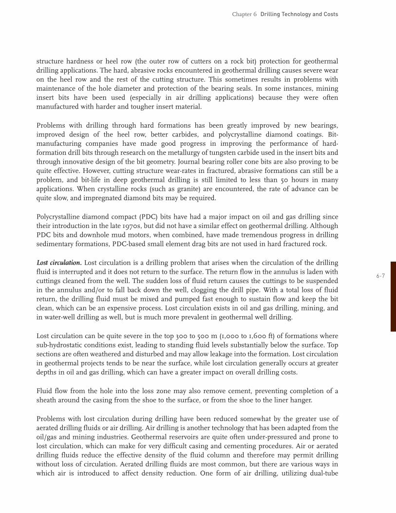
Lost circulation. Lost circulation is a drilling problem that arises when the circulation of the drilling fluid is interrupted and it does not return to the surface. The return flow in the annulus is laden with cuttings cleaned from the well. The sudden loss of fluid return causes the cuttings to be suspended in the annulus and/or to fall back down the well, clogging the drill pipe. With a total loss of fluid return, the drilling fluid must be mixed and pumped fast enough to sustain flow and keep the bit clean, which can be an expensive process. Lost circulation exists in oil and gas drilling, mining, and in waterwell drilling as well, but is much more prevalent in geothermal well drilling.
Lost circulation can be quite severe in the top 300 to 500 m (1,000 to 1,600 ft) of formations where subhydrostatic conditions exist, leading to standing fluid levels substantially below the surface. Top sections are often weathered and disturbed and may allow leakage into the formation. Lost circulation in geothermal projects tends to be near the surface, while lost circulation generally occurs at greater depths in oil and gas drilling, which can have a greater impact on overall drilling costs.
Fluid flow from the hole into the loss zone may also remove cement, preventing completion of a sheath around the casing from the shoe to the surface, or from the shoe to the liner hanger.
Problems with lost circulation during drilling have been reduced somewhat by the greater use of aerated drilling fluids or air drilling. Air drilling is another technology that has been adapted from the oil/gas and mining industries. Geothermal reservoirs are quite often underpressured and prone to lost circulation, which can make for very difficult casing and cementing procedures. Air or aerated drilling fluids reduce the effective density of the fluid column and therefore may permit drilling without loss of circulation. Aerated drilling fluids are most common, but there are various ways in which air is introduced to affect density reduction. One form of air drilling, utilizing dualtube
67
68
Chapter 6 Drilling Technology and Costs
reversecirculation drilling (and tremmie tube cementing), is being tested as a solution to severe lost circulation in the tophole interval of some wells. The dualtube process provides a path for fluids to flow down the outer annulus and air to be injected in the annulus between inner tube and the outer tube. The combined effect is to airlift the cuttings and fluids inside the inner tube. The use of tremmie tubes to place cement at the shoe of a shallow (or not so shallow) casing shoe is borrowed from waterwell and mining drilling technology. This technique is helpful in cementing tophole zones, where severe lost circulation has occurred.
Another solution to cementing problems in the presence of lost circulation is to drill beyond, or bypass, the loss zone and to cement using a technique that can prevent excessive loss. Lightweight cement, foamed cement, reverse circulation cement, and lightweight/foamed cement are developments that enable this approach to be taken. However, only lightweight cement has found widespread use. Selection of an appropriate cement is critical, because a failed cement job is extremely difficult to fix.
Directional drilling. Directionally drilled wells reach out in different directions and permit production from multiple zones that cover a greater portion of the resource and intersect more fractures through a single casing. An EGS power plant typically requires more than one production well. In terms of the plant design, and to reduce the overall plant “footprint,” it is preferable to have the wellheads close to each other. Directional drilling permits this while allowing production well bottomspacings of 3,000 ft. (900 m) or more. Selective bottomhole location of production and injection wells will be critical to EGS development as highlighted in Chapters 4 and 5.
The tools and technology of directional drilling were developed by the oil and gas industry and adapted for geothermal use. Since the 1960s, the ability to directionally drill to a target has improved immensely but still contains some inherent limitations and risks for geothermal applications. In the 1970s, directional equipment was not wellsuited to the hightemperature downhole environment. High temperatures, especially during air drilling, caused problems with directional steering tools and mud motors, both of which were new to oil and gas directional drilling. However, multilateral completions using directional drilling are now common practice for both oil and gas and geothermal applications. The development of a positive displacement downhole motor, combined with a realtime steering tool, allowed targets to be reached with more confidence and less risk and cost than ever before. Technology for reentering the individual laterals for stimulation, repair, and workovers is now in place. Directional tools, steering tools, and measurementwhiledrilling tools have been improved for use at higher temperatures and are in everyday use in geothermal drilling; however, there are still some limitations on temperatures.
6.3 Historical WellCost DataIn order to make comparisons between geothermal well costs and oil and gas well costs, a drilling cost index is needed to update the costs of drilling hydrothermal and EGS or HDR wells from their original completion dates to current values. There are insufficient geothermal wellcost data to create an index based on geothermal wells alone. The oil and gas well drilling industry, however, is a large and well established industry with thousands of wells drilled each year. Because the drilling process is essentially the same for oil, gas, and geothermal wells, the Joint Association Survey (JAS) database provides a good basis for comparison and extrapolation. Therefore, data from the JAS (API, 1976

Chapter 6 Drilling Technology and Costs
2004) were used to create a drilling index, and this index was used to normalize geothermal well costs to year 2004 U.S. $. Oil and gas well costs were analyzed based on data from the 2004 JAS for completed onshore U.S. oil and gas wells. A new, more accurate drilling cost index, called the MIT Depth Dependent (MITDD) drilling index, which takes into consideration both the depth of a completed well and the year it was drilled, was developed using the JAS database (19762004) (Augustine et al., 2006). The MITDD index was used to normalize predicted and actual completed well costs for both HDR or EGS and hydrothermal systems from various sources to year 2004 U.S. $, and then compare and contrast these costs with oil and gas well costs.
6.3.1 General trends in oil and gas wellcompletion costs
Tabulated data of average costs for drilling oil and gas wells in the United States from the Joint Association Survey (JAS) on Drilling Costs (19762004) illustrate how drilling costs increase nonlinearly with depth. Completed well data in the JAS report are broken down by well type, well location, and the depth interval to which the well was drilled. The wells considered in this study were limited to onshore oil and gas wells drilled in the United States. The JAS does not publish individual well costs due to the proprietary nature of the data. The wellcost data are presented in aggregate, and average values from these data are used to show trends. Ideally, a correlation to determine how well costs vary with depth would use individual wellcost data. Because this is not possible, average values from each depth interval were used. However, each depth interval was comprised of data from between hundreds and thousands of completed wells. Assuming the well costs are normally distributed, the resulting averages should reflect an accurate value of the typical well depth and cost for wells from a given interval to be used in the correlation.
In plotting the JAS data, the average cost per well of oil and gas wells for a given year was calculated 69 by dividing the total cost of all onshore oil and gas wells in the United States by the total number of oil and gas wells drilled for each depth interval listed in the JAS report. These average costs are tabulated in Table A.6.1 (in the Appendices) and shown in Figure 6.1 as the “JAS Oil and Gas Average” points and trend line. Wells in the 01,249 ft (0380 m) and 20,000+ ft (6100+ m) depth intervals were not included, because wells under 1,250 ft (380 m) are too shallow to be of importance in this study, and not enough wells over 20,000 ft (6,100 m) are drilled in a year to give an accurate average cost per well.
A cursory analysis quickly shows that well costs are not a linear function of depth. A high order polynomial, such as:
(61)
where is the completed well cost, is the depth of the well, and ci are fitted parameters, can be used to express well costs as a function of depth. However, it is not obvious what order polynomial would best fit the data, and any decent fit will require at least four parameters, if not more. By noting that an exponential function can be expanded as an infinite series of polynomial terms:
(62)

Chapter 6 Drilling Technology and Costs
one might be able to describe the wellcost data as a function of depth using only a few parameters. As Figure 6.1 shows, the average costs of completed oil and gas wells for the depth intervals from 1,250 feet (380 m) to 19,999 feet (6,100 m) can be described as an exponential function of depth, that is:
(63)
where only two fitted parameters, a and b1, are needed. Thus, a plot of log10(well cost) vs. depth results in a straight line:
(64)
Although there is no fundamental economic reason for an exponential dependence, the “Oil and Gas Average” trend line in Figure 6.1 shows that a twoparameter exponential function adequately describes year 2004 JAS average completed well costs as a function of depth for the depth intervals considered. The correlation coefficient (R2) value for the year 2004 JAS data, when fit to Eq. (64), was 0.968. This indicates a high degree of correlation between the log of the completed well costs and depth. Similar plots for each year of JAS report data from the years 19762003 also show high levels of correlation between the log10 of well costs and depth, with all years having an R2 value of 0.984 or higher.
An insufficient number of ultradeep wells, with depths of 20,000+ ft (6,100+ m), were drilled in 2004 to give an accurate average. Instead, a number of ultradeep well costs from 19942002 were corrected to year 2004 U.S. $ using MITDD index values (see Section 6.3.2) for the 17,50019,999 feet (5,300
610 6,100 m) depth interval and plotted in Figure 6.1. Most of the data points represent individual well costs that happened to be the only reported well drilled in the 20,000+ feet (6,100 m) depth interval in a region during a given year, while others are an average of several (two or three) ultradeep wells. Extrapolation of the average JAS line beyond 20,000 feet (6,100 m), indicated by the dashed line in Figure 6.1, is generally above the scatter of costs for these individual ultradeep wells. The ultradeep well data demonstrate how much well costs can vary depending on factors other than the depth of the well. It is easy to assume that all the depth intervals would contain similar scatter in the completed well costs.
Another possible reason for scatter in the drilling cost data is that drilling cost records are often missing important details, or the reported drilling costs are inaccurate. The available cost data are usually provided in the form of an authorization for expenditures (AFE), which gives the estimated and actual expenditures for wells drilled by a company. For example, it is not uncommon for a company to cover some of the personnel and services required in the drilling of the well in the overhead labor pool, or for materials purchased for several wells to be listed as expenses on the AFE of only one of the wells. The lack of records and concern for completeness is an incentive to have a logical method to develop a model of detailed well drillingcost expectations. Such a wellcost model attempts to account for all costs that would relate to the individual well, estimated in a manner similar to a small company’s accounting.

JAS Oil and Gas AverJAS Ultra Deep Oil aThe Geysers ActualImperial Valley ActualOther Hydrothermal AHydrothermal PredictHDR/EGS ActualHDR/EGS PredictedSoultz/Cooper BasinWellcost Lite Model Wellcost Lite Base Cas
Wellcost Lite Speci5000
00.1
0.3
1
3
10
30
GeothermalWell ModelPredictions
Oil and GasAverage
100
2000 4000
Depth (meters)
Com
plet
edW
ellC
osts
(Mill
ions
ofYe
ar20
04U
S$)
6000 8000 10000
10000 15000 20000 25000 30000(ft)
JAS Oil and Gas AverageJAS Ultra Deep Oil and GasThe Geysers ActualImperial Valley ActualOther Hydrothermal ActualHydrothermal Predicted
HDR/EGS ActualHDR/EGS PredictedSoultz/Cooper BasinWellcost Lite Model Wellcost Lite Base Case Wellcost Lite Specific Wells
1.
2.
Chapter 6
JAS = Joint Association Survey on Drilling Costs.
Well costs updated to US$ (yr. 2004) using index made from 3year moving average for each depth interval listed in JAS (19762004) for onshore, completed US oil and gas wells. A 17% inflation rate was assumed for years pre1976.
Drilling Technology and Costs
3. Ultra deep well data points for depths greater than 6 km are either individual wells or averages from a small number of wells listed in JAS (19942000).
4. “Other Hydrothermal Actual” data include some nonUS wells (Source: Mansure 2004).
611
Figure 6.1 Completed geothermal and oil and gas well costs as a function of depth in year 2004 U.S. $, including estimated costs from Wellcost Lite model.

Chapter 6 Drilling Technology and Costs
6.3.2 MIT Depth Dependent (MITDD) drillingcost index
To make comparisons between geothermal well costs and oil and gas well costs, a drilling cost index is needed to update the costs of drilling hydrothermal and HDR/EGS wells from their original completion dates to current values. The MIT Depth Dependent (MITDD) drilling cost index (Augustine et al., 2006) was used to normalize geothermal well costs from the past 30 years to year 2004 U.S. $. The average cost per well at each depth interval in the JAS reports (19762004) was used to create the drilling index, because the drilling process is essentially the same for oil, gas, and geothermal wells. A 17% inflation rate was assumed for pre1976 index points. Only onshore, completed oil and gas wells in the United States were considered, because all hydrothermal and HDR wells todate have been drilled onshore. A threeyear moving average was used to smooth out shortterm fluctuations in price. The index was referenced to 1977, which is the first year for which a moving average could be calculated using data reported by JAS from the previous and following years. Previous indices condense all information from the various depth intervals into a single index number for each year. This biases the indices toward the cost of shallower wells, which are normally drilled in much larger numbers each year, and also makes them prone to error in years where a disproportionate number of either deep or shallow wells are drilled. The MITDD drilling index was chosen because it avoids these pitfalls by incorporating both depth and year information into the index. Although this method requires slightly more information and more work, it results in superior estimates of normalized drilling costs.
The MIT Depth Dependent drilling cost index is tabulated in Table A.6.2 and shown in Figure 6.2, which clearly illustrates how widely the drilling indices vary among the different depth intervals. Before 1986, the drilling cost index rose more quickly for deeper wells than shallower wells. By 1982, the index for the deepest wells is almost double the index for shallow wells. After 1986, the index for 612 shallow wells began to rise more quickly than the index for deeper wells. By 2004, the index for wells in the 1,2502,499 ft (380760 m) range is 25%50% greater than all other intervals. Although it has the same general trend as the MITDD index, the composite index (MIT Composite) – made by calculating the average cost per well per year as in previous indices – does not capture these subtleties. Instead, it incorrectly over or underpredicts wellcost updates, depending on the year and depth interval. For example, using the previous method, the index would incorrectly overpredict the cost of a deep well drilled in 1982 by more than 20% when normalized to year 2004 U.S. $. The MITDD indices are up to 35% lower for wells over 4 km (13,000 ft) deep in 2004 than the previous index. The often drastic difference between index values of the MIT Composite index – based on average costs and the new MITDD index shown in Figure 6.2 from two given years – demonstrates the superiority of the new MITDD index as a means for more accurately updating well costs.

600
500
400
Dri
llin
gC
ostI
ndex
Year
300
200
100
1975 1980 1985 1990 1995 2000 20050
MITDD Drilling Cost Index1977 = 100
1250-24992500-37493750-49995000-74997500-999910000-1249912500-1499915000-1749917500-19999MIT Composite IndexD
epth
Inte
rval
s(F
eet)
Chapter 6 Drilling Technology and Costs
Figure 6.2 MITDD drilling cost index made using average cost per well for each depth interval from Joint Association Survey on Drilling Costs (19762004), with data smoothed using a threeyear moving average 613 (1977 = 100 for all depth intervals). Note: 1 ft = 0.3048 m.
Although the drilling cost index correlates how drilling costs vary with depth and time, it does not provide any insights into the root causes for these variations. An effort was made to determine what factors influence the drilling cost index and to explain the sometimes erratic changes that occurred in the index. The large spikes in the drilling index appearing in 1982 can be explained by reviewing the price of crude oil imports to the United States and wellhead natural gas prices compared to the drilling cost index, as shown in Figures 6.3 and 6.4. The MIT Composite drilling index was used for simplicity. Figures 6.3 and 6.4 show a strong correlation between crude oil prices and drilling costs. This correlation is likely due to the effect of crude oil prices on the average number of rotary drilling rigs in operation in the United States and worldwide each year, shown in Figure 6.5. Therefore, the drilling cost index maximum in 1982 was in response to the drastic increase in the price of crude oil, which resulted in increased oil and gas exploration and drilling activity, and a decrease in drilling rig availability. By simple supplyanddemand arguments, this led to an increase in the costs of rig rental and drilling equipment. The increase in drilling costs in recent years, especially for shallow wells, is also due to decreases in rig availability. This effect is not apparent in Figure 6.5, however, because very few new drilling rigs have been built since the mid 1980s. Instead, rig availability is dependent, in part, on the ability to salvage parts from older rigs to keep working rigs operational. As the supply of salvageable parts has decreased, drilling rig rental rates have increased. Because most new rigs are constructed for intermediate or deep wells, shallow well costs have increased the most. This line of reasoning is supported by Bloomfield and Laney (2005), who used similar arguments to relate rig availability to drilling costs. Rig availability, along with the nonlinearity of well costs with depth, can account for most of the differences between the previous MIT index and the new depthdependent indices.

600
500
400
Dri
llin
gC
ostI
ndex
Valu
e
Year
Cru
deO
ilP
rice
($/b
arre
l)&
Nat
ural
Gas
Pri
ce($
/Ten
Thou
sand
Ft3 )
300
200
100
1972 1977 1982 1987 1992 1997 20020
60
50
40
30
20
10
0
MIT Composite Drilling Cost IndexCrude Oil PricesNatural Gas Price, Wellhead
Chapter 6 Drilling Technology and Costs
Figure 6.3 Crude oil and natural gas prices, unadjusted for inflation (Energy Information Administration, 2005) compared to MIT Composite Drilling Index.
614 250
200
Dri
llin
gC
ostI
ndex
Valu
e
Year
Cru
deO
ilP
rice
($/b
arre
l)&
Nat
ural
Gas
Pri
ce($
/Ten
Thou
sand
Ft3 )
150
100
50
1972 1977 1982 1987 1992 1997 20020
25
20
15
10
5
0
MIT Composite Drilling Cost IndexCrude Oil PricesNatural Gas Price, Wellhead
Figure 6.4 Crude oil and natural gas prices, adjusted for inflation (Energy Information Administration, 2005) compared to MIT Composite Drilling Index.

Chapter 6 Drilling Technology and Costs
6000
5000
4000
Rig
Cou
nt
Year
3000
2000
1000
1975 1980 1985 1990 1995 2000 20050
United StatesWorldwide
Figure 6.5 Average operating rotary drilling rig count by year, 19752004 (Baker Hughes, 2005). 615
The effect of inflation on drilling costs was also considered. Figure 6.6 shows the gross domestic product (GDP) deflator index (U.S. Office of Management and Budget, 2006), which is often used to adjust costs from year to year due to inflation, compared to the MITDD drilling cost index. Figure 6.6 shows that inflation has been steadily increasing, eroding the purchasing power of the dollar. For the majority of depth intervals, the drilling cost index has only recently increased above the highs of 1982, despite the significant decrease in average purchasing power. Because the MITDD index does not account for inflation, this means the actual cost of drilling in terms of present U.S. dollars had actually decreased in the past two decades until recently. This point is illustrated in Figure 6.7, which shows the drilling index adjusted for inflation, so that all drilling costs are in year 2004 U.S. $. For most depth intervals shown in Figure 6.7, the actual cost of drilling in year 2004 U.S. $ has dropped significantly since 1981. Only shallower wells (1,2502,499 feet) (380760 m) do not follow this trend, possibly due to rig availability issues discussed above. This decrease is likely due to technological advances in drilling wells – such as better drill bits, more robust bearings, and expandable tubulars – as well as overall increased experience in drilling wells.

600
500
400
Dri
llin
gC
ostI
ndex
&G
DP
Def
lato
rIn
dex
Year
300
200
100
1975 1980 1985 1990 1995 2000 20050
MITDD Drilling Cost IndexUnadjusted for Inflation1977 = 100
2500-37495000-749910000-1249915000-17499
1250-24993750-49997500-999912500-1499917500-19999
Depth Intervals (Feet)
GDP Deflator Index
Chapter 6 Drilling Technology and Costs
Figure 6.6 MITDD drilling cost index compared to GDP deflator index for 19772004 (U.S. Office of Management and Budget, 2006). Note: 1 ft = 0.3048 m.
250
200
Dri
llin
gC
ostI
ndex
Year
150
100
50
1975 1980 1985 1990 1995 2000 20050
MITDD Drilling Cost IndexAdjusted for Inflation1977 = 100
2500-37495000-749910000-1249915000-17499
1250-24993750-49997500-999912500-1499917500-19999
Depth Intervals (Feet)616
Figure 6.7 MITDD drilling cost index made using new method, adjusted for inflation to year 2004 U.S. $. Adjustment for inflation made using GDP Deflator index (1977 = 100). Note: 1 ft = 0.3048 m.

Chapter 6 Drilling Technology and Costs
6.3.3 Updated geothermal well costs
The MITDD drilling cost index was used to update completed well costs to year 2004 U.S. $ for a number of actual and predicted EGS/HDR and hydrothermal wells.
Table A.6.3 (see appendix) lists and updates the costs of geothermal wells originally listed in Tester and Herzog (1990), as well as geothermal wells completed more recently. Actual and predicted costs for completed EGS and hydrothermal wells were plotted and compared to completed JAS oil and gas wells for the year 2004 in Figure 6.1. Actual and predicted geothermal well costs vs. depth are clearly nonlinear. No attempt has been made to add a trend line to this data, due to the inadequate number of data points.
Similar to oil and gas wells, geothermal well costs appear to increase nonlinearly with depth (Figure 6.1). However, EGS and hydrothermal well costs are considerably higher than oil and gas well costs – often two to five times greater than oil and gas wells of comparable depth. It should be noted that several of the deeper geothermal wells approach the JAS Oil and Gas Average. The geothermal well costs show a lot of scatter in the data, much like the individual ultradeep JAS wells, but appear to be generally in good agreement, despite being drilled at various times during the past 30 years. This indicates that the MITDD index properly normalized the well costs.
Typically, oil and gas wells are completed using a 6 3/4” or 6 1/4” bit, lined or cased with 4 1/2” or 5” casing that is almost always cemented in place, then shot perforated. Geothermal wells are usually completed with 10 3/4” or 8 1/2” bits and 9 5/8” or 7” casing or liner, which is generally slotted or perforated, not cemented. The upper casing strings in geothermal wells are usually cemented all the way to the surface to prevent undue casing growth during heat up of the well, or shrinkage during 617 cooling from injection. Oil wells, on the other hand, only have the casing cemented at the bottom and are allowed to move freely at the surface through slips. The higher costs for larger completion diameters and cement volumes may explain why, in Figure 6.1, well costs for many of the geothermal wells considered – especially at depths below 5,000 m – are 25 times higher than typical oil and gas well costs.
Largediameter production casings are needed to accommodate the greater production fluid flow rates that characterize geothermal systems. These larger casings lead to larger rig sizes, bits, wellhead, and bottomhole assembly equipment, and greater volumes of cement, muds, etc. This results in a well cost that is higher than a similardepth oil or gas well where the completed hole diameter will be much smaller. For example, the final casing in a 4,000 m oil and gas well might be drilled with a 6 3/4” bit and fitted with 5” casing; while, in a geothermal well, a 10 5/8” bit run might be used into the bottomhole production region, passing through a 11 3/4” production casing diameter in a drilled 14 3/4” wellbore.
This trend of higher costs for geothermal wells vs. oil and gas wells at comparable depths may not hold for wells beyond 5,000 m in depth. In oil and gas drilling, one of the largest variables related to cost is well control. Pressures in oil and gas drilling situations are controlled by three methods: drilling fluid density, wellhead pressure control equipment, and well design. The well design change that is most significant when comparing geothermal costs to oil and gas costs is that extra casing strings are added to shut off highpressure zones in oil and gas wells. While overpressure is common in oil and gas drilling, geothermal wells are most commonly hydrostatic or underpressured. The

Chapter 6 Drilling Technology and Costs
primary wellcontrol issue is temperature. If the pressure in the well is reduced suddenly and very high temperatures are present, the water in the hole will boil, accelerating the fluid above it upward. The saturation pressure, along with significant water hammer, can be seen at the wellhead. Thus, the most common method for controlling pressure in geothermal wells is by cooling through circulation. The need for extra casing strings in oil wells, as depth and the risk of overpressure increases, may cause the crossover between JAS oil and gas well average costs and predicted geothermal well costs seen in Figure 6.1 at 6,000 m. Because no known geothermal wells have been drilled to this depth, a cost comparison of actual wells cannot be made.
The completed wellcost data (JAS) show that an exponential fit adequately describes completed oil and gas well costs as a function of depth over the intervals considered using only two parameters. The correlation in Figure 6.1 provides a good basis for estimating drilling costs, based on the depth of a completed well alone. However, as the scatter in the ultradeep wellcost data shows, there are many factors affecting well costs that must be taken into consideration to accurately estimate the cost of a particular well. The correlation shown in Figure 6.1 has been validated using all available EGS drilling cost data and, as such, serves as a starting point or base case for our economic analysis. Once more specific design details about a well are known, a more accurate estimate can be made. In any case, sensitivity analyses were used to explore the effect of variations in drilling costs from this base case on the levelized cost of energy (see Section 9.10.5).
6.4 Predicting Geothermal Well Costs with the Wellcost Lite Model
618 There is insufficient detailed cost history of geothermal well drilling to develop a statistically based cost estimate for predicting well costs where parametric variations are needed. Without enough statistical information, it is very difficult to account for changes in the production interval bit diameter and the diameter, weight, and grade of the tubulars used in the well, as well as the depths in a given geological setting. Although the correlation from the JAS data and drilling cost index discussed above allow one to make a general estimate of drilling costs based on depth, they do not explain what drives drilling costs or allows one to make an accurate estimate of drilling costs once more information about a drilling site is known. To do this, a detailed model of drilling costs is necessary. Such a model, called the Wellcost Lite model, was developed by B. J. Livesay and coworkers (Mansure et al., 2005) to estimate well costs based on a wide array of factors. This model was used to determine the most important driving factors behind drilling costs for geothermal wells.
6.4.1 History of the Wellcost Lite model The development of a wellcost prediction model began at Sandia in 1979 with the first wellcost analysis being done by hand. This resulted in the CarsonLivesayLinn SAND 812202 report (Carson, 1983). The eight generic wells examined in the model represented geothermal areas of interest at the time. The handcalculated models were used to determine well costs for the eight geothermal drilling areas. This effort developed an early objective look at the major cost categories of well construction.
The initial effort was followed by a series of efforts in support of DOE wellcost analysis and costofpower supply curves. About 1990, a computerbased program known as IMGEO (Petty, Entingh, and Livesay, 1988; Entingh and McLarty, 1991), which contained a wellcost predictive model, was

Chapter 6 Drilling Technology and Costs
developed for DOE and was used to evaluate research and development needs. The IMGEO model included cost components for geological studies, exploration, development drilling, gathering systems, power facilities, and poweronline. IMGEO led to the development of the Wellcost1996 model. As a part of the Advanced Drilling Study (Pierce et al., 1996), a more comprehensive costing model was developed, which could be used to evaluate advanced drilling concepts. That model has been simplified to the current Wellcost Lite model.
6.4.2 Wellcost Lite model description
Wellcost Lite is a sequential event and direct costbased model. This means that time and costs are computed sequentially for all events that occur in the drilling of the well. The well drilling sequence is divided into intervals, which are usually defined by the casing intervals, but can be used where a significant change in formation drilling hardness occurs. Current models are for 4, 5, and 6 intervals – more intervals can be added as required.
The model calculates the cost of drilling by casing intervals. The model is EXCEL spreadsheetbased and allows the input of a casing design program, rate of penetration, bit life, and trouble map for each casing interval. The model calculates the time to drill each interval including rotating time, trip time, mud, and related costs and endofinterval costs such as casing and cementing and well evaluation. The cost for materials and the time required to complete each interval is calculated. The time is then multiplied by the hourly cost for all rig timerelated cost elements such as tool rental, blowout preventers (BOP), supervision, etc. Each interval is then summed to obtain a total cost. The cost components of the well are presented in a descriptive breakdown and on the typical authorization for expenditures (AFE) form used by many companies to estimate drilling costs.
619
6.5 DrillingCost Model Validation 6.5.1 Basecase geothermal wells
The cost of drilling geothermal wells, including enhanced geothermal wells and hot dry rock wells exclusive of well stimulation costs, was modeled for similar geologic conditions and with the same completion diameter for depths between 1,500 and 10,000 m. The geology was assumed to be an interval of sedimentary overburden on top of hard, abrasive granitic rock with a bottomhole temperature of 200°C. The rates of penetration and bit life for each well correspond to drilling through typical poorly lithified basin fill sediments to a depth of 1,000 m above the completion interval, below which granitic basement conditions are assumed. The completion interval varies from 250 m for a 1,500 m well to 1,000 m for wells 5,000 m and deeper. The casing programs used assumed hydrostatic conditions typical for geothermal environments. All the well plans for determining base costs with depth assume a completion interval drilled with a 10 5/8” bit. The wells are not optimized for production and are largely trouble free. For the basecase wells at each depth, the assumed contingency is 10%, which includes noncatastrophic costs for troubles during drilling.
The well costs that are developed for the EGS consideration are for both injectors and producers. The upper portion of the cased production hole may need to accommodate some form of artificial lift or pumping. This would mean that the production casing would be run as a liner back up to the point at which the larger diameter is needed. Current technology for shaft drive pumps limits the setting depths to about 600 m (2,000 ft). If electric submersible pumps are to be set deeper in the hole, the required diameter will have to be accommodated by completing the well with liners, leaving greater

620
Chapter 6 Drilling Technology and Costs
clearance deeper into the hole. The pump cavity can be developed to the necessary depth. The estimates are for an injection well that has a production casing from the top of the injection zone to the surface.
EGS well depths beyond 4,000 m (13,100 ft) may require casing weights and grades that are not widely available to provide the required collapse and tensile ratings. The larger diameters needed for highvolume injection and production are also not standard in the oil and gas industry – this will cause further cost increases. Both threaded and welded connections between casing lengths will be used for EGS applications and, depending on water chemistry, special corrosionresistant materials may be needed.
An appropriately sized drilling rig is selected for each depth using the mast capacity and rig horsepower as a measure of the needed size. A rig rental rate, as estimated in the third quarter of 2004, is used in determining the daily operating expense. It is assumed that all wellcontrol equipment is rented for use in the appropriate interval. Freight charges are charged against mobilization and demobilization of the blowoutpreventer equipment.
The rates of penetration (ROP) selected in the base case are those of mediumhardness sedimentary formations to the production casing setting depth. An expected reduction in ROP is used through the production interval. For other lithology columns, it is only necessary to select and insert the price and performance expectations to derive the well cost. These bitperformance values are slightly conservative.
The 1,500 m (4,900 ft), 2,500 m (8,200 ft), and 3,000 m (9,800 ft) wellcost estimates from the model compare favorably with actual geothermal drilling costs for those depths. The deeper wells at depths of 4,000 m (13,100 ft), 5,000 m (16,400 ft), and 6,000 m (19,700 ft) have been compared to costs from the JAS oil and gas well database. The length of open hole for the 7,500 m and 10,000 mdeep wells was assumed limited to between 2,100 m (6,900 ft) and 2,600km (8,500 ft).
All wells should have at least one interval with significant directional activity to permit access to varied targets downhole. This directional interval would be either in the production casing interval or the interval just above. The amount and type of directional well design can be accommodated in the model. The wellcost estimates are initially based on drilling hardness, similar to those used in the Basin and Range geothermal region. It is assumed that the EGS production zone is crystalline. The well should penetrate into the desired temperature far enough so that any upward fracturing does not enter into a lower temperature formation. Also, each well is assumed to penetrate some specific depth into the granitic formation. In the deeper wells, a production interval of 1,000 m (3,300 ft) is assumed. It is reduced for the shallower wells and is noted in the Wellcost Lite output record
Well costs were estimated for depths ranging from 1,500 m to 10,000 m. The resulting curves indicate drilling costs that grow nonlinearly with depth. The estimated costs for each of these wells are given in Table 6.1.

Chapter 6 Drilling Technology and Costs
Table 6.1 EGS well drillingcost estimates from the Wellcost Lite model (in 2004 U.S. $)
Shallow Mid Range Deep Depth, m No. of Cost, Depth, m No. of Cost, Depth, m No. of Cost, (ft) Casing million $ (ft) Casing million $ (ft) Casing million $
Strings Strings Strings
1,500
(4,900) 4 2.3 4,000
(13,100) 4 5.2 6,000
(19,700) 5 9.7
2,500
(8,200) 4 3.4 5,000
(16,400) 4 7.0 6,000
(19,700) 6 12.3
3,000
(9,800) 4 4.0 5,000
(16,400) 5 8.3 7,500
(24,600) 6 14.4
10,000 6 20.0
(32,800)
Shallow EGS wells. For the shallow wells (1,500 m, 2,500 m, and 3,000 m), the wellcost predictions are supported by actual geothermal drilling costs from the Western U.S. states. Due to the confidential nature of these actual costs, the level of validation with the model is far from precise, because only the depth and cost were provided. No specific formation characteristics or well/casing design information was used in this modeling effort, but it was assumed that bit performance in the model was similar to current geothermal well experience.
Midrange EGS wells. For the midrange of depths, 4,000 m and 5,000 m, the cost estimates have been made by extending the same well design and drilling approaches used in the shallow group. 621
The 5,000 m well is first modeled as a 4casing interval model (surface casing, intermediate liner, production casing into the heat, production zone lined with perforated liner). Another 5 kmdeep well has 5 casing intervals (surface casing, intermediate liner, intermediate liner 2, production casing into the heat, production zone lined with perforated liner). The cost impact of the additional liner is significant. For the same diameter in the production zone, all casings and liners above that zone are notably larger in diameter.
Deep EGS wells. The 6,000 m well is the first in a number of modeled well designs with very large upper casing sections and higher cost. The 6,000 m well uses 5 and 6casing interval cost models to better accommodate the greater casing diameters needed and reduce the length of the intervals. The change results in an increase in cost, due to the additional casing and cementing charges as well as the other endofinterval activities that occur. The cost of a 6casing, 6,000 m (19,700 ft) geothermal well compares satisfactorily with a limited number of oil and gas wells from the JAS database. The estimated cost of the 6,000 km EGS well is $12.28 million vs. an average JAS oil and gas well cost of $18 million.
For the very deep wells, 7,500 m and 10,000 m (24,600 ft and 32,800 ft), both modeled assuming 6 casing intervals, the developed estimates reflect the extreme size of the surface casing when the amount of open hole is limited to 2,130 to 2,440 m (7,000 to 8,000 ft). The well designs were based on oil and gas experience at these depths. Wellcost models have been developed for numerous

Chapter 6 Drilling Technology and Costs
geothermal fields and other specific examples. They are in reasonable agreement with current welldrilling practice. For example, costs for wells at The Geysers and in Northern Nevada and the Imperial Valley are in good agreement with the cost models developed in this study.
6.5.2 Comparison with geothermal wells
Predicted EGS well costs (from the Wellcost Lite model) are shown in Figure 6.1, alongside JAS oil/gas well costs and historical geothermal wellcost data. For depths of up to about 4,000 m, predicted well costs exceed the oil and gas average but agree with the higher geothermal wellcost data. Beyond depths of 6,000 m, predictions drop below the oil and gas average but agree with costs for ultradeep oil and gas wells within uncertainty, given the considerable scatter of the data. The Wellcost Lite predictions accurately capture a trend of nonlinearly increasing costs with depth, exhibited by historical well costs.
Figure 6.8 shows predicted costs for hypothetical wells at completion depths between 1,500 m and 10,000 m. Cost predictions for three actual existing wells are also shown, for which real ratesofpenetration and casing configurations were used in the analysis. These wells correspond to RH15 at Rosemanowes, GPK4 at Soultz, and Habanero2 at Cooper Basin. It should be noted that conventional U.S. cementing methods were assumed, which does not reflect the actual procedure used at GPK4. Two cost predictions were made for this particular well: one (shown in Figure 6.8) based on actual recorded bit run averages, and a second (not shown) that took the best available technology into consideration. Use of the best available technology resulted in expected savings of 17.6% compared to a predicted cost of $6.7 million when the recorded bit run averages were used to calculate the estimated well cost. Figure 6.8 also includes the actual troublefree costs from GPK4 and
622 Habanero2, which agree with the model results within uncertainty. For example, the predicted cost of U.S. $ 5.87 million for Habanero2 is quite close to the reported actual well cost of U.S. $ 6.3 million (AUS $8.7 million). Both estimated and actual costs shown in Figure 6.8 are tabulated in Table A.6.3. The agreement between the Wellcost Lite predictions and the historical records demonstrate that the model is a useful tool for predicting actual drilling costs with reasonable confidence.
6.5.3 Comparison with oil and gas wells
Comparisons between cost estimates of the basecase geothermal wells to oil and gas wellcost averages are inconclusive and are not expected to yield valuable information. Oil and gas well costs over the various depth intervals range from less expensive to more expensive than the geothermal well costs developed from Wellcost Lite. However, an example wellcost estimate was developed for a 2,500 m (8,200 ft) oil and gas well with casing diameters that are more representative of those used in oil and gas drilling (the comparison is shown in Table 6.2). These costs are within the scatter of the JAS cost information for California. A 2,500 m well is a deep geothermal well but a shallow West Texas oil or gas well. This comparison shows the effect of well diameter on drilling costs and demonstrates why geothermal wells at shallow depths tend to be considerably more expensive than oil and gas wells of comparable depth.

Chapter 6 Drilling Technology and Costs
Wellcost Lite Predictions – Base Case Well CostsWellcost Lite Predictions – Actual WellReal Life Trouble Free Well Costs – Actual Wells
Cooper BasinHabanero-2
RosemanowesSoultz GPK4
20
18
16
14
12
10
8
6
4
2
00 2000 4000
Depth (meters)
Com
plet
edW
ellC
osts
(Mill
ions
ofYe
ar20
04U
S$)
6000 8000 10000
Figure 6.8 EGS wellcost predictions from the Wellcost Lite model and historical geothermal well costs, at various depths.
623
Table 6.2 Wellcost comparison of EGS with oil and gas. Costs shown are for completed through/perforated inplace casing.
Well type Depth Production casing size Final bit diameter Cost/days of drilling
EGS 2,500 m (8,200 ft) 11 3/4” 10 5/8” $3,400 m / 43
Oil / Gas average 2,500 m (8,200 ft) 8 5/8” 6 3/4” $1,800 m / 29
Oil / Gas Slim Hole 2,500 m (8,200 ft) 5 1/2” 6 3/4” $1,400 m / 21
6.5.4 Model input parameter sensitivities and drillingcost breakdown
The Wellcost Lite model was used to perform a parametric study to investigate the sensitivities of model inputs such as casing configuration, rateofpenetration, and bit life. Welldrilling costs for oil, gas, and geothermal wells are subdivided into five elements: (i) prespud costs, (ii) casing and cementing costs, (iii) drillingrotating costs, (iv) drillingnonrotating costs, and (v) trouble costs. Prespud costs include movein and moveout costs, site preparation, and well design. Casing and cementing costs include those for materials and those for running casing and cementing it in place. Drillingrotating costs are incurred when the bit is rotating, including all costs related to the rateofpenetration, such as bits and mud costs. Drillingnonrotating costs are those costs incurred when the bit is not rotating, and include tripping, well control, waiting, directional control, supervision, and well evaluation. Unforeseen trouble costs include stuck pipe, twistoffs, fishing, lost circulation, holestability problems, wellcontrol problems, casing and cementing problems, and directional problems.

624
Chapter 6 Drilling Technology and Costs
The contribution of each major drilling cost component is shown in Figure 6.9 over a range of depths. Rotatingdrilling costs and casing/cementing costs dominate well costs at all depths. Drillingrotating, drillingnonrotating, and prespud expenses show linear growth with depth. Casing/cementing costs and trouble costs increase considerably at a depth of about 6,000 m, coinciding with the point where a change from three to four casing strings is required. All of these trends are consistent with the generally higher risks and more uncertain costs that accompany ultradeep drilling.
All costs are heavily affected by the geology of the site, the depth of the well, and to a lesser degree, the well diameter. Casing and cementing costs also depend on the fluid pressures encountered during drilling. Well depth and geology are the primary factors that influence drilling nonrotating costs, because they affect bit life and therefore tripping time. Prespud costs are related to the rig size, which is a function of the well diameter, the length of the longest casing string, and the completed well depth.
Geology/RateofPenetration. Rateofpenetration (ROP), which is controlled by geology and bit selection, governs rotatingdrilling costs. EGS wells will typically be drilled in hard, abrasive, hightemperature formations that reduce ROP and bit life. This also affects drilling nonrotating costs, because lower bit life creates an increased need for trips. However, most EGS sites will have at least some softer sedimentary rock overlying a crystalline basement formation. In the past 15 to 20 years, dramatic improvements in bit design have led to much faster ratesofpenetration in hard, hightemperature environments.
The degree to which the formation geology affects total drilling costs was investigated by using the model to make wellcost predictions under four different assumed geologic settings. Rateofpenetration (ROP) and bitlife input values to the model were adjusted to simulate different drilling environments, which ranged from very fast/nonabrasive to very hard/abrasive. The medium ROP represents sedimentary basin conditions (e.g., at Dixie Valley), whereas the very low ROP would be more representative of crystalline formations such as those found at Rosemanowes. In all cases, the best available bit technology was assumed. A 4,000 mdeep well was modeled to study the impact of increasing ROP on total well cost. An 83% increase in ROP from “very low” to “medium” values resulted in a 20% cost savings.

Chapter 6 Drilling Technology and Costs
0$0
$1,000
$2,000
$3,000
$4,000
$5,000
$6,000
$7,000
$8,000
$9,000
2000
Pre-spud ExpensesCasing and CementingDrilling-RotatingDrilling-Non-rotatingTrouble
4000 6000 8000 10000 12000Depth (meters)
Cos
tper
Wel
l(Th
ousa
nds
ofU
S$)
Figure 6.9 Breakdown of drilling cost elements as a function of depth from Wellcost Lite model results.
Number of Casing Strings. A greater number of casing strings results in higher predicted drilling costs. It is not just the direct cost of additional strings that has an effect; there are also costs that occur
625 because of welldiameter constraints. For example, to maintain a 9 5/8” completion diameter – which may be required to achieve flow rates suitable for electric power production – the surface casing in a 10,000 mdeep EGS well must have a diameter of 42”. The ability to handle this large casing size requires more expensive rigs, tools, pumps, compressors, and wellhead control equipment.
The relationship between the number of casing strings and completed well costs is shown in Figure 6.10. Increasing the number of casing strings from four to five in the 5,000 mdeep well results in an 18.5% increase in the total predicted well cost. An increase in the number of casing strings from five to six in the 6,000 mdeep well results in a 24% increase in total cost. As the number of casing strings increases, the rate at which drilling costs increase with depth also increases.

Chapter 6 Drilling Technology and Costs
3000$4,000
$16,000
$14,000
$12,000
$10,000
$8,000
$6,000
4 Casing Strings5 Casing Strings6 Casing Strings
4000 5000 6000 7000 8000Depth (meters)
Com
plet
edW
ellC
ost(
Thou
sand
sof
US$
)
Figure 6.10 Change in Wellcost Lite model predictions as a function of depth and number of casing intervals.
Figure 6.11 compares rotating time with tripping time for different depths of completion, using the Wellcost Lite model. Both grow almost linearly with depth, assuming ROP and bit life remain constant. However, these may not be appropriate assumptions at greater depths.
626
00
500
1,000
1,500
2,000
2,500
2000
Tripping TimeRotating Time
4000 6000 8000 10000 12000Depth (meters)
Tim
e(H
ours
)
Figure 6.11 Comparison of rotating and tripping hours as a function of well depth from Wellcost Lite model.

Chapter 6 Drilling Technology and Costs
6.6 Emerging Drilling Technologies Given the importance of drilling costs to the economic viability of EGS, particularly for mid to lowgrade resources where wells deeper than 4 km will be required, it is imperative that new technologies are developed to maximize drilling capabilities (Petty et al., 1988; Petty et al., 1991; Petty et al., 1992; Pierce and Livesay, 1994; Pierce and Livesay, 1993a; Pierce and Livesay, 1993b). Two categories of emerging technologies that would be adaptable to EGS are considered: (i) evolutionary oil and gas welldrilling technologies available now that are adaptable to drilling EGS wells, and (ii) revolutionary technologies not yet available commercially.
6.6.1 Current oil and gas drilling technologies adaptable to EGS
There are a number of approaches that can be taken to reduce the costs of casing and cementing deep EGS wells: expandable tubular casings, lowclearance well casing designs, casing while drilling, multilaterals, and improved ratesofpenetration are developments that will dramatically improve the economics of deep EGS wells. The first three concepts, which relate to casing design, are widely used in the oil and gas industry and can easily be adapted for EGS needs. The use of multilaterals to reduce the cost of access to the reservoir has also become common practice for hydrothermal and oil/gas operations. Adaptation, analysis, and testing of new technologies are required to reduce deep EGS well costs.
Expandable tubulars casing. Casing and cementing costs are high for deep wells due to the number of casing strings and the volume of cement required. A commercially available alternative is to use expandable tubulars to line the well. Further development and testing is still needed to ensure the reliability of expandable tubular casing in wells where significant thermal expansion is expected. 627 Efforts are underway to expand the range of available casing sizes and to develop effective tools and specialized equipment for use with expandable tubulars (Benzie et al., 2000; Dupai et al., 2001; Fillipov et al., 1999).
The expandable tubing casing process utilizes a product, patented by Shell Development (Lohbeck, 1993), which allows in situ plastic deformation of the tubular casing. The interval is drilled using a bit just small enough to pass through the deepest casing string. There is an underreamer behind the lead bit. The underreamer is used to widen the bottom of the well and allow cementing of the casing, after running and expanding. The result is that the inner surfaces of adjacent casings are flush (i.e., the inner diameter is constant with depth). This allows two possible approaches to be taken: (i) the resulting casing may be used as the production string; and (ii) a liner may be run and cemented in the well after progress through the production interval is completed. Technology improvements are needed if this approach is to be taken in deep, largediameter EGS wells.
Underreamers. Monobore designs that use expandable tubulars require underreamers. The use of underreamers is common in oil and gas drilling through sediments, and provides cementing clearance for casing strings that would not otherwise be available. However, highquality underreamers for hard rock environments are not common, with expansion arms often being subject to failure. Currently, underreaming in oil and gas operations utilizes bicenter bits and PDCtype cutters. Unfortunately, the success of PDC cutters in geothermal environments has not yet been established. More robust underreamers are required for EGS applications.

Chapter 6 Drilling Technology and Costs
Lowclearance casing design. An alternative approach to using expandable tubulars is to accept reduced clearances. A well design using smaller casing and less clearance between casing strings may be appropriate (Barker, 1997). This may also require the use of an underreamer to establish clearance between the casing and the borehole for cementing. Although closer tolerances may cause problems with cementing operations, this can usually be remedied by the use of underreamers before cementing.
Drillingwithcasing is an emerging technology that has the potential to reduce cost. This approach may permit longer casing intervals, meaning fewer strings – and, therefore, reduced costs (Gill et al., 1995). Research is needed to improve our understanding of cementing practices that apply to the drillingwithcasing technique. As with expandable tubulars, the development of reliable underreamers is key to the advancement of this technology.
Multilateral completions/stimulating through sidetracks and laterals. Tremendous progress has been made in multilateral drilling and completions during the past 10 years. However, pressurebased stimulation of EGS reservoirs may still prove difficult, unless the most sophisticated (Class 5 and Class 6) completion branch connections are used. The successful development of reliable reentry schemes and innovative ways to sequentially stimulate EGS development sets may be necessary, if the additional cost of such sophisticated completion practices is to be avoided.
Well design variations. Considerable savings are possible if the length of casing intervals is extended. This will reduce the number of casing strings, and therefore, the diameter of the surface and first intermediate casings. The success of this approach depends on the ability to maintain wellbore stability of the drilled interval and to install a good cement sheath. There may be isolated intervals where this technique will be appropriate.
628
6.6.2 Revolutionary drilling technologies
Rateofpenetration issues can significantly affect drilling costs in crystalline formations. ROP problems can cause wellcost increases by as much as 15% to 20% above those for more easily drilled Basin and Range formations.
Although we have not formally analyzed the potential cost reductions of revolutionary drilling technologies as a part of this assessment, it is clear that they could have a profound longterm impact on making the lowergrade EGS resource commercially accessible. New drilling concepts could allow much higher rates of penetration and longer bit lifetimes, thereby reducing rig rental time, and lighter, lowercost rigs that could result in markedly reduced drilling cost. Such techniques include projectile drilling, spallation drilling, laser drilling, and chemical drilling. Projectile drilling consists of projecting steel balls at high velocity using pressurized water to fracture and remove the rock surface. The projectiles are separated and recovered from the drilling mud and rock chips (Geddes and Curlett, 2006). Spallation drilling uses hightemperature flames to rapidly heat the rock surface, causing it to fracture or “spall.” Such a system could also be used to melt nonspallable rock (Potter and Tester, 1998). Laser drilling uses the same mechanism to remove rock, but relies on pulses of laser to heat the rock surface. Chemical drilling involves the use of strong acids to break down the rock, and has the potential to be used in conjunction with conventional drilling techniques (Polizzotti et al., 2003). These drilling techniques are in various stages of development but are not yet commercially available. However, successful development of any of these technologies could cause a major change in drilling practices, dramatically lower drilling costs – and, even more important, allow deeper drilling capabilities to be realized.

Chapter 6 Drilling Technology and Costs
6.7 ConclusionsWellcost Lite is a detailed accounting code for estimating drilling costs, developed by B. J. Livesay and Sandia National Laboratories over the past 20 years. Wellcost Lite, which has been used to evaluate technology impacts and project EGS well costs, was used to estimate costs covering a range of depths from 1,500 m to 10,000 m. Three depth categories have been examined in some detail in this study: shallow wells (1,5003,000 m depths), midrange wells (4,0005,000 m depths), and deep wells (5,00010,000 m depths).
The shallow set of wells at depths of 1,500 m (4,900 ft), 2,500 m (8,200 ft), and 3,000 m (9,800 ft) is representative of current hydrothermal well depths. The predicted costs from the Wellcost Lite model were compared to actual EGS and hydrothermal shallow well drillingcost records that were available. The agreement is satisfactory, although actual cost data are relatively scarce, making a direct comparison not entirely appropriate.
The same welldesign concepts used for the shallow set of wells was also adopted for the midrange set, which comprised wells at depths of 4,000 m and 5,000 m (13,120 ft and 16,400 ft). There were no detailed geothermal or EGS wellcost records at these depths available for comparison with model results. Nonetheless, we believe our predicted wellcost modeling approach is conservative and, as such, produces reasonable estimates of the costs of EGS wells for 4 and 5 km drilling depths.
A similar approach was taken for the deepest set of wells at depths of 6,000 m, 7,500 m, and 10,000 m (19,700 ft, 24,600 ft, and 32,800 ft). These deeper well designs and costs are naturally more speculative than estimates for the shallower wells. There have been only two or three wells drilled close to depths of 10,000 m in the United States, so a conservative well design was used to reflect higher uncertainty.
The estimated costs for the EGS wells are shown in Table 6.1, which shows that the number of casing strings is a critical parameter in determining the well costs. Welldrilling costs have been estimated for 4, 5, and 6casing well designs. For example, Table 6.1 shows that two 5,000 m deep wells were modeled, one with 4 casing intervals and another with 5 casing intervals. The former requires fewer casing intervals but increased lengths of individual sections may raise concerns about wellbore stability. This is less of a problem if more casing strings are used, but costs will be affected by an increase in the diameter of the upper casing strings, the size of rig required, and a number of other parameters. The 6,000 m well was modeled with both 5 and 6 casing intervals. Costs for the 7,500 m and 10,000 m wells were estimated using 6 casing intervals.
Figure 6.1 shows the actual costs of geothermal wells, including some for EGS wells. The specific costs predicted by the Wellcost Lite model are plotted in hollow red diamonds (�). The modeled costs show reasonable agreement with actual geothermal well costs in the mid to deepdepth ranges, within expected ranges of variation. The agreement is not as good for shallow well costs. Also shown in Figure 6.1 are average costs for completed oil and gas wells drilled onshore in the United States, where we see an exponential dependence of cost on depth.
Emerging technologies, which have yet to be demonstrated in geothermal applications and are still going through development and commercialization, can be expected to significantly reduce the cost
629

Chapter 6 Drilling Technology and Costs
of these wells, especially those at 4,000 m depths and deeper. The technologies include those that are focused on increasing overall drill effectiveness and rates, as well as stabilizing the hole with casing, e.g., expanded tubulars, drilling while casing, enhanced underreaming, and improved drill bit design and materials. Revolutionary technologies involving a completely different mechanism of drilling and/or casing boreholes were also identified, which could ultimately have a large impact on lowering drilling costs and enabling economic access to lowgrade EGS resources.
630

Chapter 6 Drilling Technology and Costs
ReferencesAmerican Petroleum Institute (API). 19762004. “Joint Association Survey (JAS) on Drilling Costs.”Washington, D.C.
Armstead, H. C. H. and J. W. Tester. 1987. Heat Mining. E.F. Spon, London.
Augustine, C., B. Anderson, J. W. Tester, S. Petty, and W. Livesay. 2006. “A comparison of geothermalwith oil and gas drilling costs.” Proc. 31st Workshop on Geothermal Reservoir Engineering, StanfordUniversity, Stanford, Calif.
Baker Hughes. 2005. “Worldwide Right Count.” Online Posting, December.<http://www.bakerhughes.com/investor/rig>
Baria, R. 2005. MilTech UK Limited, Personal Communication, November 11.
Barker, J.W. 1997. “Wellbore Design With Reduced Clearance Between Casing Strings.” Proc.SPE/IADC Drilling Conference, SPE/IADC 37615, Amsterdam.
Batchelor, A. S. 1989. Geoscience Ltd., Falmouth, U.K., Personal Communication, December 12, 1989.
Bechtel National Inc. 1988. “Hot Dry Rock Venture Risks and Investigation,” Final report for the U.S.Department of Energy, under contract DEAC0386SF16385, San Francisco, CA.
Benzie, S., P. Burge, and A. Dobson. 2000. “Towards a MonoDiameter Well Advances in ExpandingTubular Technology.” Proc. SPE European Petroleum Conference 2000, SPE 65164, Paris.
Bloomfield, K. K. and P. T. Laney. 2005. “Estimating Well Costs for Enhanced Geothermal SystemApplications.” Report for the U.S. Department of Energy, INL/EXT0500660, under contract DEAC07051D14517, Idaho National Laboratory, Idaho Falls, Idaho. 631
Carson, C. C., Y. T. Lin, and B. J. Livesay. 1983. “Representative Well Models for Eight GeothermalResource Areas.” Sandia National Laboratories report, SAND812202.
Dupai, K. K., D. B. Campo, J. E. Lofton, D. Weisinger, R. L. Cook, M. D. Bullock, T. P. Grant, and P.L. York. 2001. “Solid Expandable Tubular Technology – A Year of Case Histories in the Drilling Environment.” Proc. SPE/IADC Drilling Conference 2001, SPE/IADC 67770.
Energy Information Administration, U.S. Department of Energy. 2005. “Section 9 Energy Prices, Tables 9.1 and 9.11,” Monthly Energy Review, September.
Entingh, D. 1987. “Historical and Future Cost of Electricity from Hydrothermal Binary and Hot Dry Rock Reservoirs, 19752000.” Meridian Corp. report 240GG, Alexandria, Va., October.
Entingh, D. 1989. Meridian Corporation, Alexandria, Va., Personal Communication, November.
Entingh, D. and L. McLarty. 1991. “Geothermal Cost of Power Model IMGEO Version 3.05: User’s Manual.” Meridian Corporation.
Filippov, A., R. Mack, L. Cook, P. York, L. Ring, and T. McCoy. 1999. “Expandable Tubular Solutions.” SPE Annual Conference and Exhibition, SPE 56500, Houston.
Geddes, C. J. and H. B. Curlett. 2006. “Leveraging a new energy source to enhance oil and oil sands production.” GRC Bulletin, January/February, pp. 3236.
Gill, D. S., W. C. M. Lohbeck, R. B. Stewart, and J. P. M van Viet. 1995. “Method of creating a casing in a borehole.” Patent No. PCT / EP 96/0000265, Filing date: 16 January 1995.

Chapter 6 Drilling Technology and Costs
Hori, Y. et al. 1986. “On Economics of Hot Dry Rock Geothermal Power Station” and related documents. Corporate Foundation Central Research Institute for Electric Power, Hot Dry Rock Geothermal Power Station Cost study Committee Report 385001, Japan.
Lohbeck, W. C. M. 1993. “Method of completing an uncased section of a borehole.”
Patent publication date: 23 December 1993.
Mansure, A. J. 2004. Sandia National Laboratories, Personal Communication, April 12.
Mansure, A. J., S. J. Bauer, and B. J. Livesay. 2005. “Geothermal Well Cost Analyses 2005.” Geothermal Resources Council Transactions, 29:515–519.
Milora, S. L. and J. W. Tester. 1976. Geothermal Energy as a Source of Electric Power. MIT Press, Cambridge, Mass.
Petty, S., D. Entingh, and B. J. Livesay. 1988. “Impact of R&D on Cost of Geothermal Power, Documentation of IMGEO Model Version 2.09.” Contractor Report, Sandia National Laboratories, SAND877018
Petty, S., B. J. Livesay, and W. P. Long. 1991. “Supply of Geothermal Power from Hydrothermal Sources.” Contractor Report, Sandia National Laboratory.
Petty, S., B.J. Livesay, W. P. Long, and J. Geyer. 1992. “Supply of Geothermal Power from Hydrothermal Sources: A Study of the Cost of Power in 20 and 40 years.” Contractor Report, Sandia National Laboratory, SAND 927302.
Pierce, K. G. and B.J. Livesay. 1994. “A Study of Geothermal Drilling and the Production of Electricity from Geothermal Energy.” Contractor Report, DOEGET and Sandia National Laboratory, SAND 921728.
632 Pierce, K.G. and B. J. Livesay. 1993a. “An Estimate of the Cost of Electricity Production from HotDry Rock.” SAND930866J.
Pierce, K. G. and B. J. Livesay. 1993b. “An Estimate of the Cost of Electricity Production from HotDry Rock.” Geothermal Resources Council Bulletin, 22(8).
Pierce, K. G., B. J. Livesay, and J. T. Finger. 1996. “Advanced Drilling Systems Study.” Sandia National Laboratories, SAND950331.
Polizzotti, R. S., L. L. Hirsch, A. B. Herhold, and M. D. Ertas. 2003. “Hydrothermal Drilling Method and System.” United States Patent No. 6.742,603, July 3.
Potter, R. M. and J. W. Tester. 1998. “Continuous Drilling of Vertical Boreholes by Thermal Processes: Including Rock Spallation and Fusion.” United States Patent No. 5,771,984, June 30.
Shock, R. A. W. 1986. “An Economic Assessment of Hot Dry Rocks as an Energy Source for the U.K.” Energy Technology Support Unit Report ETSUR34, U.K. Department of Energy, Oxfordshire, U.K.
Tester, J. W. and H. Herzog. 1990. “Economic Predictions for Heat Mining: A Review and Analysis of Hot Dry Rock (HDR) Geothermal Energy Technology.” Final Report for the U.S. Department of Energy, Geothermal Technology Division, MITEL 90001, Cambridge, Mass.
United States Office of Management and Budget (U.S. OMB). 2006. “Section 10 – Gross Domestic Product and Implicit Outlay Deflators – Table 10.1.” Budget of the United States Government, Washington, D.C.
Wyborn, D. 2005. Chief Scientific Officer, Geodynamics, Ltd., Queensland, Australia, Personal Communication, November 11.
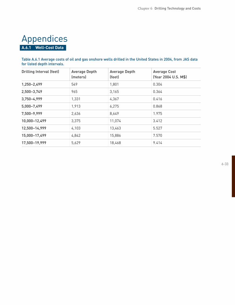
Chapter 6 Drilling Technology and Costs
AppendicesA.6.1 WellCost Data
Table A.6.1 Average costs of oil and gas onshore wells drilled in the United States in 2004, from JAS data for listed depth intervals.
Drilling Interval (feet) Average Depth Average Depth Average Cost (meters) (feet) (Year 2004 U.S. M$)
1,250–2,499 549 1,801 0.304
2,500–3,749 965 3,165 0.364
3,750–4,999 1,331 4,367 0.416
5,000–7,499 1,913 6,275 0.868
7,500–9,999 2,636 8,649 1.975
10,000–12,499 3,375 11,074 3.412
12,500–14,999 4,103 13,463 5.527
15,000–17,499 4,842 15,886 7.570
17,500–19,999 5,629 18,468 9.414
633
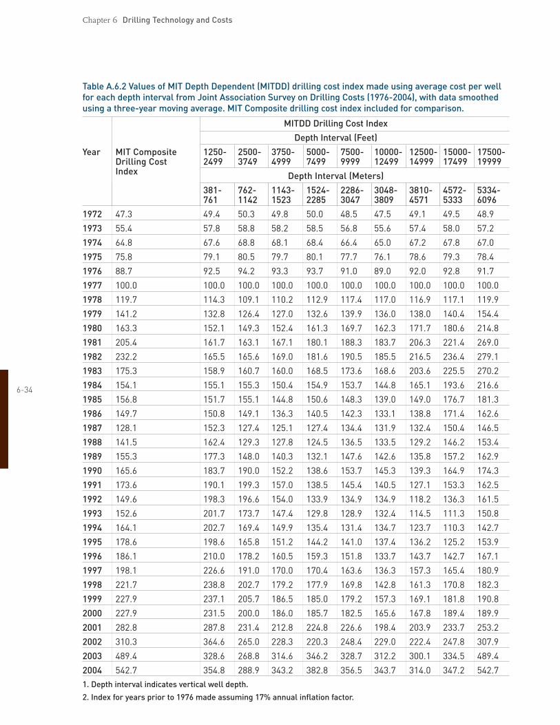
Chapter 6 Drilling Technology and Costs
Table A.6.2 Values of MIT Depth Dependent (MITDD) drilling cost index made using average cost per well for each depth interval from Joint Association Survey on Drilling Costs (19762004), with data smoothed using a threeyear moving average. MIT Composite drilling cost index included for comparison.
MITDD Drilling Cost Index
Depth Interval (Feet)
Year MIT Composite 1250 2500 3750 5000 7500 10000 12500 15000 17500Drilling Cost 2499 3749 4999 7499 9999 12499 14999 17499 19999 Index Depth Interval (Meters)
381 762 1143 1524 2286 3048 3810 4572 5334761 1142 1523 2285 3047 3809 4571 5333 6096
1972 47.3 49.4 50.3 49.8 50.0 48.5 47.5 49.1 49.5 48.9
1973 55.4 57.8 58.8 58.2 58.5 56.8 55.6 57.4 58.0 57.2
1974 64.8 67.6 68.8 68.1 68.4 66.4 65.0 67.2 67.8 67.0
1975 75.8 79.1 80.5 79.7 80.1 77.7 76.1 78.6 79.3 78.4
1976 88.7 92.5 94.2 93.3 93.7 91.0 89.0 92.0 92.8 91.7
1977 100.0 100.0 100.0 100.0 100.0 100.0 100.0 100.0 100.0 100.0
1978 119.7 114.3 109.1 110.2 112.9 117.4 117.0 116.9 117.1 119.9
1979 141.2 132.8 126.4 127.0 132.6 139.9 136.0 138.0 140.4 154.4
1980 163.3 152.1 149.3 152.4 161.3 169.7 162.3 171.7 180.6 214.8
1981 205.4 161.7 163.1 167.1 180.1 188.3 183.7 206.3 221.4 269.0
1982 232.2 165.5 165.6 169.0 181.6 190.5 185.5 216.5 236.4 279.1
1983 175.3 158.9 160.7 160.0 168.5 173.6 168.6 203.6 225.5 270.2
634 1984 154.1 155.1 155.3 150.4 154.9 153.7 144.8 165.1 193.6 216.6
1985 156.8 151.7 155.1 144.8 150.6 148.3 139.0 149.0 176.7 181.3
1986 149.7 150.8 149.1 136.3 140.5 142.3 133.1 138.8 171.4 162.6
1987 128.1 152.3 127.4 125.1 127.4 134.4 131.9 132.4 150.4 146.5
1988 141.5 162.4 129.3 127.8 124.5 136.5 133.5 129.2 146.2 153.4
1989 155.3 177.3 148.0 140.3 132.1 147.6 142.6 135.8 157.2 162.9
1990 165.6 183.7 190.0 152.2 138.6 153.7 145.3 139.3 164.9 174.3
1991 173.6 190.1 199.3 157.0 138.5 145.4 140.5 127.1 153.3 162.5
1992 149.6 198.3 196.6 154.0 133.9 134.9 134.9 118.2 136.3 161.5
1993 152.6 201.7 173.7 147.4 129.8 128.9 132.4 114.5 111.3 150.8
1994 164.1 202.7 169.4 149.9 135.4 131.4 134.7 123.7 110.3 142.7
1995 178.6 198.6 165.8 151.2 144.2 141.0 137.4 136.2 125.2 153.9
1996 186.1 210.0 178.2 160.5 159.3 151.8 133.7 143.7 142.7 167.1
1997 198.1 226.6 191.0 170.0 170.4 163.6 136.3 157.3 165.4 180.9
1998 221.7 238.8 202.7 179.2 177.9 169.8 142.8 161.3 170.8 182.3
1999 227.9 237.1 205.7 186.5 185.0 179.2 157.3 169.1 181.8 190.8
2000 227.9 231.5 200.0 186.0 185.7 182.5 165.6 167.8 189.4 189.9
2001 282.8 287.8 231.4 212.8 224.8 226.6 198.4 203.9 233.7 253.2
2002 310.3 364.6 265.0 228.3 220.3 248.4 229.0 222.4 247.8 307.9
2003 489.4 328.6 268.8 314.6 346.2 328.7 312.2 300.1 334.5 489.4
2004 542.7 354.8 288.9 343.2 382.8 356.5 343.7 314.0 347.2 542.7
1. Depth interval indicates vertical well depth.
2. Index for years prior to 1976 made assuming 17% annual inflation factor.

Chapter 6 Drilling Technology and Costs
Table A.6.3a Actual and predicted geothermal well drilling and completion costs (2004 U.S. $).
Well ID Depth Depth Cost When Year Cost Year Comments (meters) (feet) Drilled (M$) Drilled 2004 (M$)
GT1 732 2402 0.060 1972 0.66
GT2 2932 9619 1.900 1974 10.95 Fenton Hill Site,
EE1 3064 10052 2.300 1975 10.78 New Mexico, USA. Actual Costs
EE2 4660 15289 7.300 1980 12.69 (Tester and Herzog, 1990)
EE3 4250 13944 11.500 1981 19.16
EE3a 4572 15000 5.160 1988 11.08
RH11 (low) 2175 7136 1.240 1981 2.36
RH11 (high) 2175 7136 1.984 1981 3.78 Rosemanowes Site, Cornwall, UK.
RH12 (low) 2143 7031 1.240 1981 2.36 Actual Costs. (Tester and Herzog, 1990)
RH12 (high) 2143 7031 1.984 1981 3.78 Low: $1 = 1£ GBP
RH15 (low) 2652 8701 2.250 1985 5.81 High: $1.6 = 1£ GBP
RH15 (high) 2652 8701 3.600 1985 9.29
UK (Shock, 1987) 6000 19685 8.424 1985 16.13 Camborne School of Mines($1 = 1£ GBP)
Bechtel (1988) 3657 11998 3.359 1987 9.08 Predict. for Roosevelt Hot Springs, UT
Hori et al. (1986) 3000 9843 6.000 1985 15.49 Predicted Costs
Entingh (1987) I 3000 9843 6.900 1984 17.18 Predicted Costs based on
Entingh (1987) II 3000 9843 3.800 1984 9.46 Heat Mining
Entingh (1987) III 3000 9843 3.000 1984 7.47
Heat Mining 3000 9843 3.000 1984 7.47 Predicted Costs Armstead & Tester (1987) 635
The Geysers 1800 5906 0.486 1976 1.78 Actual costs Milora & Tester (1976)
The Geysers 3048 10000 2.275 1989 5.69 Actual costs Batchelor (1989)
Imperial Valley 1600 5249 0.165 1976 0.60 Actual costs Milora & Tester (1976)
IMGEO IVFL 1829 6001 1.123 1986 2.74
IMGEO IVBI 2743 8999 0.956 1986 2.57
IMGEO BRFL 2438 7999 1.217 1986 3.27
IMGEO BRBI 914 2999 0.556 1986 1.32 Meridian predictions of hydrothermal
IMGEO CSFL 3048 10000 2.032 1986 5.44 wells from IMGEO database (Entingh,
IMGEO CSBI 914 2999 0.576 1986 1.37 1989). Only base well costs shown.
IMGEO YVFL 1524 5000 0.906 1986 3.76
IMGEO YVBI 152 499 0.406 1986 1.46
IMGEO GYDS 3048 10000 1.155 1986 3.09

Chapter 6 Drilling Technology and Costs
Table A.6.3a (continued)
SNL – NonUS 2317 7603 1.539 1996 3.88
SNL – NonUS 2374 7789 1.729 1997 4.05
SNL – NonUS 2377 7800 1.377 1996 3.47
SNL – NonUS 2739 8986 1.867 1997 4.37
SNL – NonUS 2760 9055 1.320 1997 3.09
SNL – NonUS 2807 9210 2.979 1996 7.51
SNL – NonUS 2819 9249 0.915 1997 2.14 Actual geothermal well costs from
SNL – NonUS 2869 9414 1.030 1996 2.60 Sandia National Laboratories
SNL – NonUS 3021 9912 1.060 1996 2.67 (SNL) (Mansure, 2004)
SNL – NonUS 3077 10096 1.514 1996 4.04
SNL – US 2277 7471 1.186 1985 2.70
SNL – US 2334 7658 0.822 1986 2.21
SNL – US 1703 5588 0.804 1986 1.96
SNL – US 2590 8496 2.220 1991 5.85
SNL – US 2627 8618 1.760 1997 4.12
GPK3 5101 16731 6.571 2003 6.88 Soultz, France. Trouble costs excluded.
GPK4 5100 16728 5.14 2004 5.14 (1 USD = 1.13 EUD) (Baria, 2005)
Cooper Basin, 4725 15498 6.3 2004 6.3 Trouble costs excluded. Australia (1 USD = 0.724 AUD) (Wyborn, 2005) Habanero 2
636 1. M$ = millions of U.S. $.
2. A listing and discussion of the origins of many of the actual and predicted well costs is given in Tester and Herzog (1990).
3. Currency conversions based on yearly average of Interbank conversion rate.
Table A.6.3b Predicted geothermal well drilling and completion costs from Wellcost Lite model (in year 2004 U.S. $).
Well ID Depth Depth Estimated Comments
(meters) (feet) Cost (2004 M$)
WCL Base Case Well 1500 4921 2.303 Wellcost Lite (WCL) Base
WCL Base Case Well 2500 8202 3.372 Case Wells
WCL Base Case Well 3000 9842 4.022 Assume 10% Contingency
WCL Base Case Well 4000 13123 5.223 Costs
WCL Base Case Well 5000 16404 6.740
WCL Base Case Well 6000 19685 9.172
WCL Base Case Well 7500 24606 14.645
WCL Base Case Well 10000 32808 19.731
Rosemanowes 2800 9200 4.195 Estimates made using
Soultz GPK4 5100 16750 6.705 actual casing program for
Cooper Basin – Habanero2 4725 15500 5.872 specific individual wells

Chapter 6 Drilling Technology and Costs
A.6.2 Wellcost Lite Model A.6.2.1 Background and brief history of the development of Wellcost Lite
A more robust, yet easiertouse costing model, Wellcost Lite, was developed to more readily accommodate changes in the drilling system.
The Wellcost Lite model has been qualified by offering the cost estimate to someone involved in drilling that area, for their comment, agreement or disagreement. This was especially true of the earlier models. Well costs were not normally made public by the companies and, to some degree, still are not. Recently, agreements have been made between Sandia and operators to access some records. Some of these records had been kept on a RimBase format. RimBase is a cost and timeaccounting system for use on the drill rig. Records that were not initially on RimBase were handentered into the RimBase format. Reasonable agreement has been made from those records to Wellcost Lite model results.
But even with those records, an estimate for a well to be drilled with a different depth, final diameter, casing design, etc. is still needed. Comparison between Wellcost Lite modeled cost and fielddrilling numbers is an ongoing effort through Sandia.
A.6.2.2 Wellcost Lite – How does the cost model work?
Wellcost Lite is a sequential, eventbased and item costbased estimate for drilling. The model approach takes into account the time and materials cost for each action relating to the drilling of the well. The Input field acts as a reminder for each step of drilling and the cost and time involved. The Cost Information Spreadsheet retains an estimate of the cost and performance of materials and services.
637 Well design/well planning. Each cost model is constructed by developing a well design profile. Sequentially, as the well is drilled, details for each interval are entered in the Input Section and are summed into the Wellcost Section, and subsequently presented on an AFE output format or other format.
Well design is the initial step in developing the cost of an EGS well. The well design schematic and casing information is provided or developed by the modeler. The downhole geology sets (or estimates) the array of formations to be drilled in a particular well. A performance map for the well is created for bits and hole openers. With the tectonically jumbled regions, geothermal wells are very likely to vary even when close to one another. The expected downhole geological conditions are estimated from the experience of geologists and engineers familiar with the areas in question.
Well control is considered in well design, especially in the top intervals of the hole. Geothermal wellcontrol pressures are mostly determined based on the temperatures expected in the well and occasionally for artesian pressures as well. The fracture tolerance gradient of the formations is used to determine the safe depths for the surface casing and subsequent casing strings.
Experience has taught how much “open hole” can be exposed during drilling before it is necessary to run and cement casing to protect the integrity of the well. Wellbore stability can be a mechanical problem, where weak and ratty formations exist; or it can be a chemically based problem where the clays in the shales and other formations are weakened when exposed to the drilling fluid. The amount of open hole puts limits on how long an interval can be and how long it may be safe to expose the formations to the drilling fluids.

638
Chapter 6 Drilling Technology and Costs
Well depth and final drill bit diameter come into play in designing the well schematic. The schematic is a representation of the selected diameters, weights of the casing, and the grade of material used in the manufacture of the pipe. The productive interval bit diameter sets the diameters from the bottom to the surface. Geothermal wells tend to use largerdiameter casing than are used in oil and gas well completions. For the most part, K55, L80, and T95 casing grades are used in making the estimates. Available sizes and weights are determined by contacting the casing vendors.
Modeling the well cost also considers the requirements presented by the geologic stratigraphy to be drilled, the desired depth, and the final production interval bit diameter. Using these requirements, the well is designed. The traditional, casingwithinacasing design can be estimated based on the available sizes, desired clearance for cementing, and accepted risk of the amount of open hole. Normal wellbore to casing clearances in use in the geothermal drilling industry are applied wherever possible. There is some leeway in the well design where multiple casing strings are to be run.
The geothermal industry has to depend on the oil and gas drilling industry to set the available supply of casing sizes, and weights and grades of steel available for geothermal completions. Geothermal drilling has little or no impact on the available inventory. Onshore oil and gas wells tend to be smaller in diameter than geothermal wells. This sometimes puts a limitation of the availability of casing sizes, weights, and grades.
CIS 3rd Quarter 2004. The Cost Information Spreadsheet (CIS 3rd/2004) is used to set the costs of goods and services at a particular date (or period of time) and to set guidelines to be used in materials, equipment and services, time lines, performance, and cost. A file for casing cost is maintained for the different casing sizes, weights and grades, and connections. The CIS also provides for collapse calculations and costs for largediameter welded pipe used in the tophole section of the well (20” casing is the largest seamless casing normally manufactured and threaded).
Drilling costs are subjected to considerable volatility. The rig rental rate, material costs, and services are all subjected to supplyanddemand cycles that are not necessarily tied to the Consumer Price Index. There is, however, a Drilling Cost Index that reflects changes in drilling cost. But this is an annualized record and of little help if costing a current well. Unfortunately, the variations occur on a monthly rather than an annual basis. Because geothermal wells use a slightly larger selection of casing diameters, weights, and grades, the supply for geothermal may be limited. Each cost information spreadsheet (for example, CIS 3rd Quarter 2004) has a date stamp. Models have been used for 1979, 1996, 2000, third quarter 2004, and fourth quarter 2005.
Information will be entered for all drilling intervals and each subsequent “end of interval time and cost” and for the initial completion of the well.
Prespud. Prespud expenses are listed and accounted. These are expenses that are incurred before the hole is actually started (spudded). Prespud cost for the cost of mobilizing and demobilizing the rig, setting up a water supply, the drill site construction, conductor hole drilling and cementing, the well cellar, etc. are all estimated and appear in the Prespud subsection of the Input Section.
Daily operating expenses. A cost for the daily (and, therefore, hourly) cost of operations is developed by making daily cost entries for each item listed. The rig daily rental rate and the other running costs such as insurance, overhead, management, drilling engineering charges, rig supervision, and other miscellaneous timebased charges (daily or hourly operating cost) are entered for the overall

Chapter 6 Drilling Technology and Costs
operation. There is an hourly cost for the rig, for fuel for the rig (computed from horsepower rating of the rig), for a drilling supervisor, a drilling management activity, charges for insurance, power, water, etc. Some of these categories of costs are often omitted from drillingcost records. The level of detail necessary for parametric changes to the well design are often missing.
Table A.6.4 Input section, top page. Cost Information Field EGS 5000 m 16400 ft E Rev7 105/8 12/3/2005 Well Configuration Hole Dia Depths Casing Cost/ft Interval ROP Bit Life
Conductor Pipe/Line Pipe 26”bit/36”HO 80 30”0.375 Wall welded 118lb/ft $90.00 Conductor
Surface CSG 28” 1,250 22”0.625 Wall welded $107.00 1 Casing 25 90
Intermediate CSG 20” 5,000 16”109lb K55 Premium $70.86 2 Liner 25 80
Intermediate CSG 2 143/4” 13,120 113/4”73.6lb T95 Premium $78.24 3 Casing 18 65
Production Zone 103/8”special 16,400 85/8”36lb K55 slotted Butt $29.80 4 perf Liner 15 45
Prespud and Mobilization Depths Casing Frac Gradient Mud Shoe Critical psi psi/ft Pressure
0.8 9.6 Csg String
Activity Cost 80 112 psi 64 40
Mobilization $132,000 1,250 570 psi 1000 624 22”0.625lb
Mobilization Labor $16,500 5,000 3180 psi 4000 2496 16”109lb
Demobilization $66,000 13,120 5920 psi 10496 6550 113/4”73.6lb
Demobilization Labor $16,500 16,400 9320 psi 13120 8187 85/8”36lb
Waste Disposal & Cleanup $30,000 0 N/A 0
$261,000.00
Location Cost 639 Site Expense $32,000
Cellar $25,000
Drill Conductor Hole $8,000
Water Supply $10,000
Initial Mud Cost $10,000
Prespud Cost Total $85,000.00
$346,000.00
Description
Daily Operating Cost $1,040.65 $24,975.60
Rig Day Rate $687.50 $16,500.00 2,000 hp 1,200,000 mast
Fuel $1,425.60 0.45 x hp x 0.06 x cost per gal x 24 Cost Per Gallon
Water $400.00 Estimated
Electric Power $50.00 Estimated $1.10
Camp Expense $200.00 Estimated
Drilling Supervision $1,200.00 $1000/day 1 man
DRLG Engr & Management $1,000.00 Estimated
Mud Logging $1,800.00 Current Rate
Hole Insurance $250.00 Estimated
Administrative Overhead $500.00 Estimated
Misc Transportation $500.00 Estimated
Site Maintenance $200.00 Estimated
Waste Disposal and Cleanup $200.00 Estimated
Misc Services $750.00 Estimated

Chapter 6 Drilling Technology and Costs
Table A.6.5 Input section, Interval 3 example.
EGS 5000 m 16400 ft E Rev 7 105/8
Input Information Interval 3
Production Casing 143/4” Casing 113/4” 73.6lb T95 Premium $78.24
Depth of Interval 3 13120 Shoe Depth 13,120 Casing Length
Interval Length 8120 Interval Length
ROP ft/hr Bit Life Hrs No.of Bits
Bit Performance 143/4”bit 18.00 65.00 7
Hourly Rates Rig Time Charge Time Misc. Hourly One Time Explanation of Charges and Not Rig Time Expense Expenses source of Information
Delta Time Hrs 451.11 Computed Drilling Hours
Technical Changes Hrs & $
Drilling Fluids
Mud Cost $/Hr $100.00 x $45,111.11 $4000.00 Hourly Mud Expense
Mud Treatment Equip $25.00 x 451.11 $11,277.78 $1000.00 Mud Treatment Equipment
Mud Cooling Equip $20.00 x 451.11 $9,022.22 $1000.00 Mud Coolers
Air Service Hrs & $ $150.00 20.00 $3,000.00 $2,000.00 Air Drilling Services
D/H Tools and Times
BHA Changes Hrs 2 14.00 Hours to Change BHA
BIT Trips Hrs 63.42 Total Interval Trip Time
640 BITS $18,970.00 x $132,790.00 143/4”$17,000 each
Stab, Reamers, HO x $26,558.00
DRLG Tools. Jars, Shocks x $19,918.50
D/H Rentals, DP, DC, Motor x $17,000.00
Drill String Inspections x $3,000.00
Small Tools and Supplies x $5,000.00
Reaming Hrs & $ $0.00 12.00 $0.00 $4,000.00 Reaming Hrs &$
Hole Opening Hrs & $ $0.00 0.00 $0.00 $0.00 Hole Opening Hrs & $
Directional
Dir Engr Services Hrs & $ $40.00 10.00 451.11 $18,044.44 $1,200.00 Directional Drilling Expense
Dir Tools Hrs & $ $10.00 x 451.11 $4,511.11 $4,000.00 Directional Drilling Tools
Mud Motors Hrs & $ $200.00 x 451.11 $90,222.22 $1,000.00 Mud Motor Charges
Steering/MWD Equip Hrs & $ $100.00 x 451.11 $45,111.11 $1,000.00 MWD Charges
Trouble
Fishing Hrs & $ $10.00 0.00 0.00 $0.00 $1,000.00 Fishing Standby and Expenses
Lost Circulation Hrs & $ 0.00 0.00 0.00 Lost Circulation Estimated
MISC Trouble Hrs & $ 12.00 Misc Trouble Cost

Chapter 6 Drilling Technology and Costs
Table A.6.5 (continued)
EGS 5000 m 16400 ft E Rev 7 105/8
End of interval
Logging Hrs & $ 18.00 $36,000.00 Logging Time and Expense
Casing Services $ x $40,350.00 Casing Service, or Welding, and Mob.
CSG/Liner Hrs & $ 48.00 $1,026,508.80 Casing Time and Cost
Casing Cementing Equipment x $8,000.00
Liner Hanger and Packers 0.00 $0.00 Liner Hanger if used
Cementing Hrs & $ 30% excess 22.00 $40/ft3 $270,000.00 Cementing time, WOC and expense
End of Interval Hrs & $ 12.00 $20,000.00 End of Interval
Wellhead $ 8.00 $15,000.00 Well Head Cost
Welding and Heat Treat 24.00 Rental 163/4” $25,000.00 Welding and Heat Treat
BOPE Hrs & $ $1,212.00 12.00 BOPE $22,781.11 $3,000.00 BOPE Rental, Change out Time, Testing
Test and Completion Install 11” BOPE
Location Cost x $0.00
Testing Coring Sampling 0.00 $0.00
Well Testing Hrs & $ 0.00 $0.00 Well Testing Expenses
Completion Hrs & $ 12.00 $20,000.00 Valves
Production Tree and Valves 0.00 $84,000.00 Master Valves and exp 641 Spool
$249,081.11
Total Interval Rig Hours 706.53 Daily Operating $735,251.60
$1,772,325.30 $2,756,658.01

642
Chapter 6 Drilling Technology and Costs
Input Section. The Input Section acts as a reminder of each event within each interval to be accounted. A time and cost for each activity in an interval are entered. For all activities that affect the hours for the rig, the hourly operating rate is charged and tracked in the interval. All direct costs are also entered. For charges that do not affect rig hours, a charge time is developed and multiplied by the number of hours that would be charged for the rental or service. There is a running cost based on the additional equipment that is on the “clock” during drilling operations. Some of these events and equipment also require freight charges, mobilization charges (or initiation cost), and demobilization charges. Each event or equipment selection may also result in a direct cost for materials such as bits or packers or wellheads. With this degree of detail, the model can be altered to account for changes in procedures and for differences in service and equipment performances. The model can also be adapted to develop costs for alternative drilling methods and technologies. The costing process is adaptable and flexible.
At the end of these interval steps, there are a series of endofinterval activities that are listed and a cost and time recorded for each activity. That includes circulating and conditioning drilling fluid, logging the well, running casing, cementing the casing, and changing out the wellcontrol equipment to accommodate the new diameter of drilling to occur next.
The model is developed for a particular well by accounting for each time and each cost during the drilling of a well. At each step along the way, an account is kept of the amount of time required of the rig, the amount and cost of materials, and the time and cost of services to develop the well to completion.
Wellcost Section. The Wellcost Section sums the costs and times into an account for each interval. The amount of time and dollars can be determined from the Wellcost Section for each activity in each interval. It is possible to track the interval costs from beginning to end. At the end of each interval, a sum of the interval cost is available.
AFE Section. All of the costs and times are then transferred or summed to an AFE Sheet. The AFE Sheet was chosen as the primary form of output because most available information is recorded in that format. The total well cost, the time, and the cost for each major type of expense is listed in the authorization for expenditures (AFE) spreadsheet.
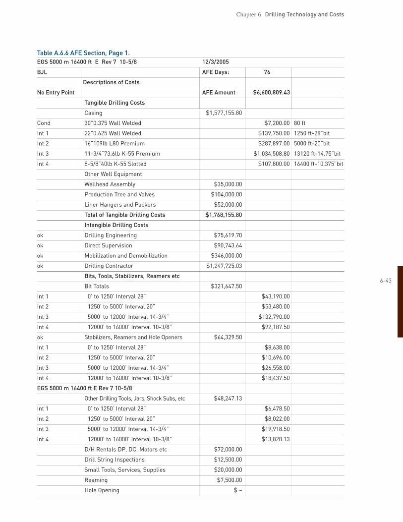
Chapter 6 Drilling Technology and Costs
Table A.6.6 AFE Section, Page 1. EGS 5000 m 16400 ft E Rev 7 105/8 12/3/2005
AFE Days: 76
$6,600,809.43
BJL
Descriptions of Costs
No Entry Point AFE Amount
Tangible Drilling Costs
Casing $1,577,155.80
Cond 30”0.375 Wall Welded $7,200.00 80 ft
Int 1 22”0.625 Wall Welded $139,750.00 1250 ft28”bit
Int 2 16”109lb L80 Premium $287,897.00 5000 ft20”bit
Int 3 113/4”73.6lb K55 Premium $1,034,508.80 13120 ft14.75”bit
Int 4 85/8”40lb K55 Slotted $107,800.00 16400 ft10.375”bit
Other Well Equipment
Wellhead Assembly $35,000.00
Production Tree and Valves $104,000.00
Liner Hangers and Packers $52,000.00
Total of Tangible Drilling Costs $1,768,155.80
Intangible Drilling Costs
ok Drilling Engineering $75,619.70
ok Direct Supervision $90,743.64
ok Mobilization and Demobilization $346,000.00
ok Drilling Contractor $1,247,725.03
Bits, Tools, Stabilizers, Reamers etc 643
Bit Totals $321,647.50
Int 1 0’ to 1250’ Interval 28” $43,190.00
Int 2 1250’ to 5000’ Interval 20” $53,480.00
Int 3 5000’ to 12000’ Interval 143/4” $132,790.00
Int 4 12000’ to 16000’ Interval 103/8” $92,187.50
ok Stabilizers, Reamers and Hole Openers $64,329.50
Int 1 0’ to 1250’ Interval 28” $8,638.00
Int 2 1250’ to 5000’ Interval 20” $10,696.00
Int 3 5000’ to 12000’ Interval 143/4” $26,558.00
Int 4 12000’ to 16000’ Interval 103/8” $18,437.50
EGS 5000 m 16400 ft E Rev 7 105/8
Other Drilling Tools, Jars, Shock Subs, etc $48,247.13
Int 1 0’ to 1250’ Interval 28” $6,478.50
Int 2 1250’ to 5000’ Interval 20” $8,022.00
Int 3 5000’ to 12000’ Interval 143/4” $19,918.50
Int 4 12000’ to 16000’ Interval 103/8” $13,828.13
D/H Rentals DP, DC, Motors etc $72,000.00
Drill String Inspections $12,500.00
Small Tools, Services, Supplies $20,000.00
Reaming $7,500.00
Hole Opening $ –

Chapter 6 Drilling Technology and Costs
Table A.6.7 AFE section, Page 2.
Directional Services and Equipment
Directional $272,975.56
Directional Engineering Service $36,451.11
Directional Tools $23,191.11
Mud Motors $140,222.22
Steering/MWD Equipment $73,111.11
Trouble
Fishing Tools and Services $5,000.00
Lost Circulation $40,000.00
Misc. Trouble Cost $ –
Drilling Fluids Related
Drilling Muds, Additives & Service $104,227.78
Mud Cleaning Equipment $25,744.44
Mud Coolers $19,395.56
Air Drilling Services and Equipment $45,500.00
Casing Cementing and EOI
Casing Tools and Services $127,060.00 644 Welding and Heat Treat $49,000.00
Cement and Cement Services $554,000.00
Mob/Demob Cementing Equipment $ –
Int 1 0’ to 1250’ Interval 28”x 22” Casing $122,000.00
Int 2 1250’ to 5000’ Interval 20”x 16” Casing $162,000.00
Int 3 5000’ to 12000’ Interval 143/4”x 113/4” Shoe to Surface $270,000.00
Int 4 No Cement Perforated Liner Perforated Liner $ –
Well Control Equipment
Blow out Preventer Rentals $48,546.67
Int 1 Diverter $3,500.00 26” to 1,000’
Int 2 211/4”2000 Stack $10,750.00 20” to 5,000’
Int 3 163/4”3000 Stack $25,781.11 143/4” to 10,000’
Int 4 135/8”3000 Stack $8,515.56 103/8” to 15,000’
Int 5 135/8”3000 Stack $ – 77/8” to 20,000

Chapter 6 Drilling Technology and Costs
Table A.6.8 AFE section, Page 3.
EGS 5000 m 16400 ft E Rev 7 105/8
Logging and Testing
ok Mud Logging and H2S Monitoring & Equip. $136,115.46
Electrical Logging $94,000.00
Int 1 0’ to 1250’ Interval $ –
Int 2 1250’ to 5000’ Interval $18,000.00
Int 3 5000’ to 12000’ Interval $36,000.00
Int 4 12000’ to 16000’ Interval $40,000.00
Int 5 16000’ to 20000’ Production Interval $ –
Testing, Sampling & Coring $2,000.00
Well Test $130,000.00
Completion Costs $95,000.00
Misc Expenses
ok Transportation and Cranes $37,809.85
ok Fuel $107,803.44
ok Water and System $30,247.88
ok Electric Power $3,780.98
Location Cost
ok Camp Cost and Living Expenses $15,123.94 645
ok Site Cleanup, Repair, Waste Disposal $15,123.94
Site Maintenance $15,123.94
Location Costs $ –
Misc Administrative and Overhead
Administrative Overhead $37,809.85
Well Insurance $18,904.92
Miscellaneious Services $56,714.77
Total Intangible Drilling Costs $4,393,321.48 75.620 days
Total Tangible Drilling Costs $1,768,155.80
Total Tangible and Intangible Costs $6,161,477.28
Contingencies 10% of Intangibles $439,332.15
Total Drilling Costs $6,600,809.43

646
Chapter 6 Drilling Technology and Costs
Trouble costs. Time and costs for troubles are entered into the Input Sections as expected. Some companies do not permit trouble cost expectations to be entered in the originating cost estimate. Separate costing modules can be created for trouble events such as lost circulation, stuck pipe, failed cement, etc. The frequency of these occurrences is more difficult to establish, because there are not enough examples to establish a statistical frequency. When trouble is to be included, interviews with individuals with knowledge of the area have been used to establish the likelihood of these trouble events. A “trouble event” time and direct cost can then be entered into Wellcost Lite Input Sheet in the appropriate interval. In many geothermal areas, for the tophole, it is common to have severe lost circulation especially above the water table. The number of events in the interval is estimated from interviews and what records are available. The degree of the trouble is also estimated. Lost circulation, stuck pipe, twistoffs, and the resulting fishing, instrumentation temperature limitations, and failed cement jobs can be significant cost items. Failed cementing jobs and collapsed casing are more complicated and difficult to properly include. For geothermal drilling records, only the identifiable troubles are listed. Trouble event times and costs can be estimated for each type and severity of problem.
Output of well costs. The output of the cost model can take a number of useful forms. The information entered into the Input Section is automatically summed in the Wellcost Section. The cost summary for each interval is available from the Wellcost Section. At the end of each interval, a total time and cost are summed and listed.
Because most drilling authorizations are put in an authorization for expenditures (AFE) format, it is used as one of the output formats for Wellcost Lite. Other formats have evolved for specific uses. The variations needed for the EGS Cost of Geothermal Power consideration were reduced to a representative curve, a simplification, for ease of use. There will be a unique curve for different geological areas.

Chapter 6 Drilling Technology and Costs
Table A.6.9 Description section, Page 1.
EGS 5000 m 16400 ft E Rev 7 105/8 12/3/2005
$6,600,809 Total Well Cost w/cont
$6,161,477 Total Well Cost wo/cont
$346,000 Prespud
$2,593,216 Well Construction
$1,768,156 Tangible
$825,060 Non Tangible Well Construction Expenses
$3,222,261 Drilling
$2,508,886 Drilling Hole Making Related
$223,078 Mgmt and Overhead
$83,182 Site Related
$45,000 Trouble Cost
$362,115 Evaluation
$6,161,477 Chk Sum should Equal Total wo/cont
$391 Total w/contprespud/depth
$162 Well Construction/depth 647
$363 Total wo/contprespud/depth
$229 Drilling+Contingency/depth
$229 Total w/contprespudconstruction/depth
1,815 Total Hours
76 Days
870 Rotating Hours 47.9%
179 Tripping Hours 9.9%

Chapter 6 Drilling Technology and Costs
26” bit36” hole
30” casing
16” casing
casing
22” welded
20” bit26” bit
20” bit
14-3/4” bit
10-5/8” bit
11-3/4” casing
8-5/8” slotted liner
16” casing
5000
14-3/4” bit
11-3/4” casing
10-5/8” bit8-5/8” slotted
5000
10000
11000
12000
13120
16400
13000
14000
15000
16000
22” csg1250
5000 m / 4 casing 5000 m / 5 casing
648
Figure A.6.1 4 and 5interval 5,000 m casing

Chapter 6 Drilling Technology and Costs
A.6.3 Model Results for Specific Areas and Depths
Wells selected to represent potential U.S. EGS sites have been cost estimated using the Wellcost Lite modeling technique with the same performance parameters and cost values from earlier work reported. The variations in depth and bit performance have been an input for each model. The list of U.S. EGS sites is preliminary, but well cost can be estimated for any site that is chosen. The specific U.S. EGS sites well costs are as follows:
a. East Texas – NW LA / E Texas Basin
Well cost
Well design reservoir temperature
Formations
Bit performance
$7,665,032 / 69 days of drilling
200°C
Sandstone grading to harder sediments
Sediment to the hot zone, then altered sediments
Casing shoe
TD
13,350 ft
16,400 ft
Openhole interval 3,050 ft
b. SE Idaho – N Utah / Ore Ida
Well cost
Well design reservoir temperature
Formations
$6,993,136 / 81 days of drilling
265°C
Basalt to 1,500 m 649
Bit performance Crystalline to 4,500 ft (1,500 m), then alteredsediments, followed by crystalline
Casing shoe 14,100 ft
TD 16,400 ft, 5,0004
Openhole interval 2,300 ft
The Ore Ida well is estimated using the 5,0004 well, since it is thought that wellbore stability will not be a significant problem in that area. If wellbore stability is a perceived problem, then the cost would be greater.
c. NE Montana / Poplar Dome
Well cost
Well design reservoir temperature
Formations
$3,166,027 / 37 days of drilling
135°C
Madison limestone, sandstone, limestone and shale
Bit performance
Casing shoe
TD
Altered sediment throughout
6,200 ft
7,200 ft
Openhole interval 1,000 ft

Chapter 6 Drilling Technology and Costs
d. Northern California / Clear Lake
Well cost $10,670,125 / 115 days of drilling 5 intervals / no stability problems
Well cost $13,305,073 / 126 days of drilling 6 intervals / concern for stability problems
Well design reservoir temperature 415°C
Formations Granite, rhyolite, hydrothermally altered metasediments
Bit performance Altered sediment for top 5,000 ft to 9,000 ft, then granite
Casing shoe 15,800 ft
TD 19,700 ft
Openhole interval 3,900 ft
The Clear Lake prospective site will differ by almost $3 million, depending on the amount of ash or unstable zones that are encountered. For an unstable geology, the greater cost should be used.
e. SE Oregon / Sisters Area
Well cost $7,243,690 / 87 days of drilling
Well design reservoir temperature 225°C
650 Formations Granite, tuffs, andesite, andesite/basaltic lavas
Bit performance Use altered sediment and crystalline ROP and hrs
Casing shoe 13,120 ft
TD 16,400 ft
Openhole interval 3,280 ft
f. New Hampshire / Conway Granite
Well cost
Well design reservoir temperature
Formations
$15,570,743 / 154 days of drilling
200°C
Granite from surface down
Bit performance
Casing shoe
TD
Use crystalline ROP and hrs
18,400 ft
23,000 ft
Openhole interval 4,600 ft
The bit performance values used in the EGS wells have been assumed to be slower and with fewer hours due to the depth of drilling. The bit performance map used for the New Hampshire well assumes crystalline formations from the surface down.

Chapter 6 Drilling Technology and Costs
A.6.4 Model Results for Reworked Wells
The least expensive rework will be to extend the depth of the well while the rig is still mobilized over the hole, and before the perforated liner has been run in the shorter interval.
A planned multilateral would mean sidetracking out of the well from a zone shallower than the original leg of the well. If it is necessary to sidetrack from a shallower point in search of promising fractures, then the cost to cement, pull back, and sidetrack the well will be more significant. This effort is a remedial operation to enhance the production. This cost would be similar to a multilateral additional cost. The rig on reworks and remedial operations will be costestimated for the 5,000 m (16,400 ft) wells using the 4 and 5interval models.
A.6.4.1 Rig on drilling / deepening 460 m (1,500 ft) / rig still on the well
The cost increment for drilling an additional 460 m (1,500 ft) is $375,000 (5,000 m well). This is a simple extension of the final interval, using the same ROP/hrs performance numbers and addition length to the perforated liner. The rig is over the hole, so there is no mobilization charge. Procuring and having the extra length of perforated liner would not be a significant planning issue.
A.6.4.2 Rig on drilling / sidetracked lateral / as a planned part of the well design
To sidetrack the well as a planned part of the well, the kickoff point would be 645 m (2,120 ft) above the last casing point of 4,000 m (13,120 ft for a 5,000 m /16,400 ft well) at 3,355 m (11,000 ft). With a build rate of 3°/100 ft of measured depth, 305 m (1,000 ft) of drilling would set the angle at 30 degrees. Drilling another 1,145 m (3,754 ft) would be the middle of the 1,000 m (3,280 ft) hot zone. Drilling would proceed to a total measured depth of 5,380 m (17,648 ft). The sidetracked lateral would
651have penetrated completely through the hot zone. The Total Vertical Depth at the 5,380 m (17,648 ft) measured depth would be 5,000 m (16,400 ft). The horizontal departure would be 650 m (2,132 ft). The planned lateral will be used to develop a second production (or injection) leg to the well.
Using the 5,0004 model without the sidetrack was $6,989,859, which took 1,960 hours in 82 days. The total well cost with the additional sidetracked interval would cost $8,972,859, done in 2,827 hours in 118 days. This is an additional cost of $1,983,000 and 36 days.
A.6.4.3 Reworks / rig has to be mobilized / add a lateral for production maintenance / a workover
A well recompletion, which requires a lateral to restore production flow or temperature, would then require an additional $400,000 for mobilization/demobilization, blowout preventer equipment (BOPE) rental, and setup. Due to the depth, the rig would need to be of a similar size and specification. The configuration of the well would be the same as the sidetracked lateral noted above. There would be an additional cost of $90,000 for a bridge plug and cement. The whipstock is covered in the above cost model. The total for the lateral, as a remedial operation, would cost $2,473,000 and take approximately 40 days. It is assumed that the formations being drilled are mostly crystalline.
A.6.4.4 Redrills to enhance production / a workover / rig to be mobilized
To deepen a 5,000 m (16,400 ft) well by 1,500 ft to 17,900 ft, which requires the mobilization of a rig, is considerably more expensive. There will be a cost of $500,000 for mobilization/demobilization, BOPE rental, and setup. The total cost of the deepening by 457 m (1,500 ft) would be $900,000.

Chapter 6 Drilling Technology and Costs
Almost any workover that requires mobilizing a rig will run between $700,000 and $1 million, depending on the depth of the well being reworked. The cost of a coiled tubing rig for this operation is only marginally less expensive, because coiled tubing rigs have gotten quite expensive.
Maintenance reworks for acidizing, casing scraping, logging, etc. will be in the same range of $600,000 to $1 million per well event.
652