FACULTY OF SCIENCE AND TECHNOLOGY

MASTER'S THESIS

Study program/specialization:

Petroleum Engineering - Drilling & Well

Technology

Spring semester, 2009

Open

Author: Morten Kartevoll

………………………………………… (signature author)

Instructor:

Erik Skaugen

Supervisor(s):

Arne Valland Singelstad and Tor Henry Omland

Title of Master's Thesis: Drilling problems in depleted reservoirs

ECTS: 30

Subject headings:

- Depleted zones

- ECD

- Wellbore pressure

- Specific case history

Pages: 33

Stavanger, ………………..

Date/year

1

Drilling problems in depleted reservoirs

Morten Kartevoll

Spring semester, 2009

Petroleum Engineering - Drilling & Well Technology

Universitetet i Stavanger

In collaboration with

StatoilHydro

2

Abstract

When drilling a well there are several factors involved governing the pressure measured

downhole. Being able to predict and control these in addition to having an understanding of

the formation being drilled makes it possible to drill in environments that were not possible

to drill with yesterday’s technology.

This paper gives an introduction to the rock mechanics of a formation and explains what

parameters are involved at governing the bottomhole pressure in a well. Pore pressure

prediction, fracture pressure estimation as well as a description of equivalent circulation

density and the challenges of drilling in a pressure depleted formation are also discussed.

A case study from a field in the North Sea is included. This was the main motivation for

writing this thesis. In order to look at a field case and draw conclusions based on

observations require knowledge about what caused that which is observed. The case is a

well drilled in the North Sea in 2006 which experienced a severe loss of circulation incident.

No direct cause of this incident was found during an investigation performed by

StatoilHydro. This paper looks at different possible causes with supporting evidence and

presents a recommendation of what could be done to prevent similar incidents in the future.

All data from the field and the well has been anonymized after wishes from StatoilHydro and

partners.

3

Table of contents

1. ACKNOWLEDGEMENTS 4

2. INTRODUCTION 5

3. THEORY 6

3.1 Rock mechanics 6

3.2 Pore pressure prediction 9

3.3 Fracture pressure prediction 9 3.3.1 Leak-off test (LOT) and extended leak-off test (XLOT) 10

3.4 Equivalent circulation density 11

3.5 Drilling in depleted zones 13 3.5.1 Heterogeneous depletion 13 3.5.2 Managed Pressure Drilling 15

3.6 Wellbore pressure 15 3.6.1 Fluid friction 16 3.6.2 Cuttings 17 3.6.3 Drillstring rotation and eccentricity 18 3.6.4 Tool joints 21 3.6.5 Lateral drillstring movement 21

4. CASE HISTORY - A LOSS OF CIRCULATION INCIDENT IN THE NORTH SEA 22

4.1 Underestimated depletion 22

4.2 Shear tension in the formation 24

4.3 Pack off 24

4.4 Stringer penetration 25

4.5 Drilling fluid properties 26

5. DISCUSSION 29

6. CONCLUSION 31

7. REFERENCES 32

4

1. Acknowledgements

I would like to thank Professor Erik Skaugen at UiS for all his help while I was writing my

master thesis. I would also like to thank StatoilHydro for giving me the opportunity to use

their facilities and giving me access to relevant data for my work. Special thanks go to Arne

Valland Singelstad, Tor Henry Omland, Ståle Østensen and Frode Robberstad for helping me

out with technical and theoretical questions and feedback.

5

2. Introduction

New oil and gas wells are becoming more challenging to drill. New technology and better

understanding of new and existing reservoirs become available, pushing the envelope of

what is technically possible and economically viable. When new technology makes difficult

wells possible to drill, more data is needed. Better understanding of what affects the drilling

process is crucial in order to make the operation as efficient and safe as possible

A lot of the new wells drilled today go into or through zones in the formation that have

already been produced from. The reason for this could be that an existing reservoir needs to

be drained from a different location in order to enhance the hydrocarbon recovery. Or it

could that a new reservoir located below an older one is discovered or has not been possible

to reach before. Lower pore pressure than what used to be present is encountered and this

gives rise to problems and potential risks that have to be dealt with.

When a formation is depleted from earlier fluid extraction, the operating window between

the pore pressure and the fracture pressure for the section gets narrower. Due to these

smaller tolerances, variations in drilling parameters will have a bigger impact on the

downhole conditions. Knowing how different parameters will affect the downhole pressure

is of great help. This aids in the design of a drilling program that can get a section drilled as a

whole while minimizing the risk for operational hazards.

6

3. Theory

3.1 Rock mechanics

For prediction of formation behavior, models are needed to predict the stress, strain and

pressure development in the wellbore. The simplest model, which assumes linear elastic and

isotropic properties and no geological processes making any directional dependent tension,

can be used as an analogy. In this model it is only the vertical tension, the overburden, which

causes horizontal tensions, which are equal in all directions.

Stress is defined as force acting through a cross section. Depending on the orientation of the

force to the cross section the stress is called normal stress or shear stress.

Fig 3.1: A force is shown going through three different cross sections. The planes a) and b) experience normal

stress while c) has shear stress[1]

.

Normal stress, denoted σ, is given by this equation[1]:

A

F=σ (1)

Shear stress, which is present in Fig. 3.1 at point c), is a decomposition of the force. The

component acting normal on the cross section is the normal stress portion, while the

component acting parallel with the cross section is the shear stress part, denoted τ[1].

A

FP=τ (2)

Strain, ε, is defined as an elongation in positive or negative direction of a material due to the

forces acting on it. Poisson’s ratio is the strain in y direction divided by the strain in x

direction, see Fig. 3.2. The two are calculated by the following equations[1]:

L

L

L

LL ∆=−= 'ε (3)

7

x

y

εε

υ −= (4)

The negative sign in equation (4) is used to maintain a positive sign convention for the

Poisson’s ratio.

Fig 3.2: A body in two dimensions is shown where a force is applied, deforming the body. It becomes shorter

in x direction and wider in y direction[1]

.

Using Hooks law in a Cartesian coordinate system with the axes x, y and z gives the following

equations[1, 2]:

)( zyxxE σσνσε +−= (5)

)( xzyyE σσνσε +−= (6)

)( yxzzE σσνσε +−= (7)

E = modulus of elasticity

ν = Poisson’s ratio

εx, εy, εz = relative change in length in directions x, y and z

σx, σy, σz = formation stress in directions x, y and z

However, in rock mechanics we use other denotations for the formation tensions. σx, σy and

σz will hereafter be denoted σH, σh and σv respectively, where σH is the largest horizontal

stress, σh the least, and σv is the overburden.

We further assumed that the formation in question is a non porous one, like salt or granite.

This means the overburden σv is given by the following[2]:

ghgh Fwwv ρρσ += (8)

σv = overburden

ρw = density of seawater

hw = sea depth

ρF = average density of the formation

h = depth, starting from the seabed

g = constant of acceleration (9,81 m/s2)

8

Given the statement that no geological process is to be taken into account the horizontal

tensions σH and σh are equal and there is no change in lengths in these directions, so εx = εy =

0. By inserting this into Hook’s law we get:

vHvHHvhHxE νσσνσσνσσσνσε −−=+−=+−== )1()()(0

vhH σν

νσσ−

==⇒1

(9)

vvHvHHvzE σν

νσνσσσσνσε−

−=−=+−=1

22)(

2

E

vz

σν

νε

−−=⇒

1

21

2

(10)

Equations (9) and (10) give the horizontal tension in the formation and how much the

formation have been squeezed together in vertical direction because of the overburden,

respectively. As long as the assumptions made previously is applied to any formation, the

horizontal tension in any direction will be equal to σH = σh.

If σH and σh are not equal, the coordinate system has to be arranged such that the axis are

along the principal stresses. When this is done, the horizontal stress in any direction can be

calculated.

If the formation is porous, the pores will most likely contain water with a (pore) pressure PP.

The pore pressure will reduce the vertical tension in the formation, because it is carrying

some of the load from the overburden, and the change in tension is σv - PP. Still having the

assumption that there are no geological effects on tension, equation (9) will for a porous

formation give this result:

)(1 PvPhPH PPP −

−=−=− σ

ννσσ

PvPPvhHF PPPPννσ

ννσ

ννσσ

−−+

−=+−

−===⇒

1

21

1)(

1 (11)

PF = fracture pressure

PP = pore pressure

The fracture pressure is the minimum pressure needed in the well to break or tear up the

formation around the wellbore. Natural fractures present in the formation will be held shut

by the horizontal stresses. If the fluid pressure is higher than the horizontal stress, which is

the stress in the formation itself and the pore pressue, the fracture will open. This is also

dependent on the fluids ability to get into the fractures, so if a good mud cake is present a

higher fracture pressure will be seen than if an inferior one is.

9

3.2 Pore pressure prediction

Pore pressure (PP) is an important parameter in rock mechanics as it will carry part of the

total stresses in a porous, fluid-filled rock system. It’s a well documented fact that porous

and permeable formations obey an effective stress law[1]:

PPP Pασσ −=' (12)

σ’P = effective external hydrostatic stress

σP = external hydrostatic stress

α = Biot factor (≈ 1 in weak or unconsolidated formations)

The properties of the formation are governed by the effective stress, so it is important to

know the PP present. In a saturated formation, assuming that the fluid in the pores can

migrate to the surface at the same rate as the rate of compaction, PP will develop as a

normal gradient governed by the weight of the fluid column[1]:

gdzzPD

fPn )(0∫= ρ (13)

PPn = normal pore pressure

ρf = fluid density, dependent on salinity

z = depth

There are several different cases where the PP does not follow the normal gradient. If the

rate of sedimentation and compaction is higher than the migration rate for pore fluid it will

lead to a higher PP than what would be expected. Other reasons for having abnormally high

PP could be tectonic loading causing shear stress with associated increase in PP and thermal

or chemical processes leading to fluid expansion or generation respectively. However if the

PP is lower than expected this is often the result of pore fluid extraction from the formation

(see section about drilling in depleted zones).

When PP gradients are made, information about the formation fluids and tectonics are

needed. Combined with information from adjacent wells such as; pressure readings,

reservoir models, formation type and depletion factors, this help to create a predictive PP

gradient for the location of interest.

3.3 Fracture pressure prediction

To determine the smallest horizontal stress, σh, the formation is fractured and the pressure

when the fracture closes is measured. To get reliable measurements it is important that the

fractures have propagated far enough into the formation so that all factors/elements from

the wellbore stresses can be neglected. For a vertical well this is obtained when the fracture

length is two to three wellbore diameters. For a deviated well the fracture may have to

travel farther away to encounter only the in-situ stresses due to a more complicated stress

regime around the wellbore.

10

3.3.1 Leak-off test (LOT) and extended leak-off test (XLOT)

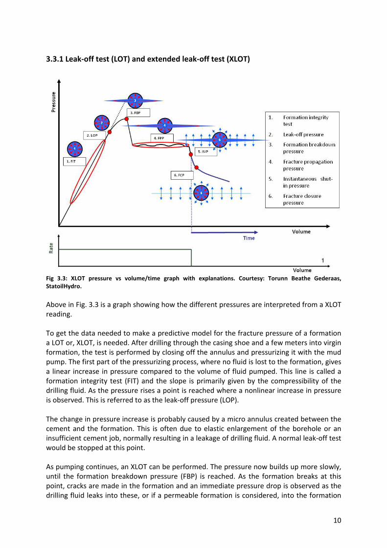
Fig 3.3: XLOT pressure vs volume/time graph with explanations. Courtesy: Torunn Beathe Gederaas,

StatoilHydro.

Above in Fig. 3.3 is a graph showing how the different pressures are interpreted from a XLOT

reading.

To get the data needed to make a predictive model for the fracture pressure of a formation

a LOT or, XLOT, is needed. After drilling through the casing shoe and a few meters into virgin

formation, the test is performed by closing off the annulus and pressurizing it with the mud

pump. The first part of the pressurizing process, where no fluid is lost to the formation, gives

a linear increase in pressure compared to the volume of fluid pumped. This line is called a

formation integrity test (FIT) and the slope is primarily given by the compressibility of the

drilling fluid. As the pressure rises a point is reached where a nonlinear increase in pressure

is observed. This is referred to as the leak-off pressure (LOP).

The change in pressure increase is probably caused by a micro annulus created between the

cement and the formation. This is often due to elastic enlargement of the borehole or an

insufficient cement job, normally resulting in a leakage of drilling fluid. A normal leak-off test

would be stopped at this point.

As pumping continues, an XLOT can be performed. The pressure now builds up more slowly,

until the formation breakdown pressure (FBP) is reached. As the formation breaks at this

point, cracks are made in the formation and an immediate pressure drop is observed as the

drilling fluid leaks into these, or if a permeable formation is considered, into the formation

11

itself. The pressure drops until it becomes constant and the fracture propagation pressure

(FPP) is obtained.

While still pumping drilling fluid, the cracks will continue to open more and more in a

stepwise manner, hence the reason for the observed fluctuation in the FPP. After the FPP

has been measured for a given volume of drilling fluid, typically around 1,5m3, the pumps

are stopped. An immediate pressure drop due to the ceasing of the frictional pressure loss is

observed and this is denoted as the instantaneous shut-in pressure (ISIP). The pressure in

the well will continue to drop and the fracture closure pressure (FCP) is found. If the

formation is permeable, the FCP is the breakpoint in the pressure vs. the square root of time

curve. If the formation is impermeable the drilling fluid in the cracks is bleed off through a

constant choke, and the FCP is the breakpoint in the pressure vs. flowback volume curve.

These two interpretations should give compatible FCPs.

The FCP is interpreted as the σh and it is recommended to set this as the maximum value for

the static mud weight, as static losses then will be omitted. The σH is usually found by using a

relation model, with data from a LOT or XLOT as input. Finally the fracture pressure curve

presented in the pressure plots is set as a value 5-10% higher than σH calibrated with other

data available. The fracture pressure is usually set as the highest limit for the ECD in the well.

3.4 Equivalent circulation density

The equivalent circulation density can be interpreted as the density of a fluid, which in static

conditions and at a depth of interest produces the same pressure as a given drilling fluid in

dynamic conditions[3].

ECD is presented as a dimensionless pressure gradient. In order to present the pressure drop

in the wellbore as ECD it needs to be converted. This can be done by rearranging Eq. (12)

with respect to ρ and adding the increase in pressure due to non static conditions:

gh

PPECD

w

∆+==ρρ

(14)

ECD = dimensionless number

ρ = density of a static fluid yielding the same pressure drop as a dynamic system (kg/l)

ρw = density of water (kg/l)

P = static hydraulic pressure (kPa)

ΔP = increase in pressure due to drilling operations (kPa)

g = constant of acceleration (9,81 m/s2)

h = TVD of point of interest (m)

The ECD gradient is often referred to as specific gravity (SG). That means the density of the

hypothetical fluid is divided by the density of water as a reference. By doing this it makes

calculations from SG to any other unit of density very easy, since the density used for water

is 1000 kg / m3.

When calculating the theoretical pressure drop in an annulus, all the different contributing

factors can be calculated one by one and then summed up in the ΔP term in Eq. (14). It must

12

be kept in mind that this will be an approximation of an approximation, since several of the

different factors can and will influence each other.

The ECD is not necessarily largest at the bottom of the well, this is because ECD relies on the

total pressure drop at a point in the well and the TVD of this point. This is illustrated in the

following figure:

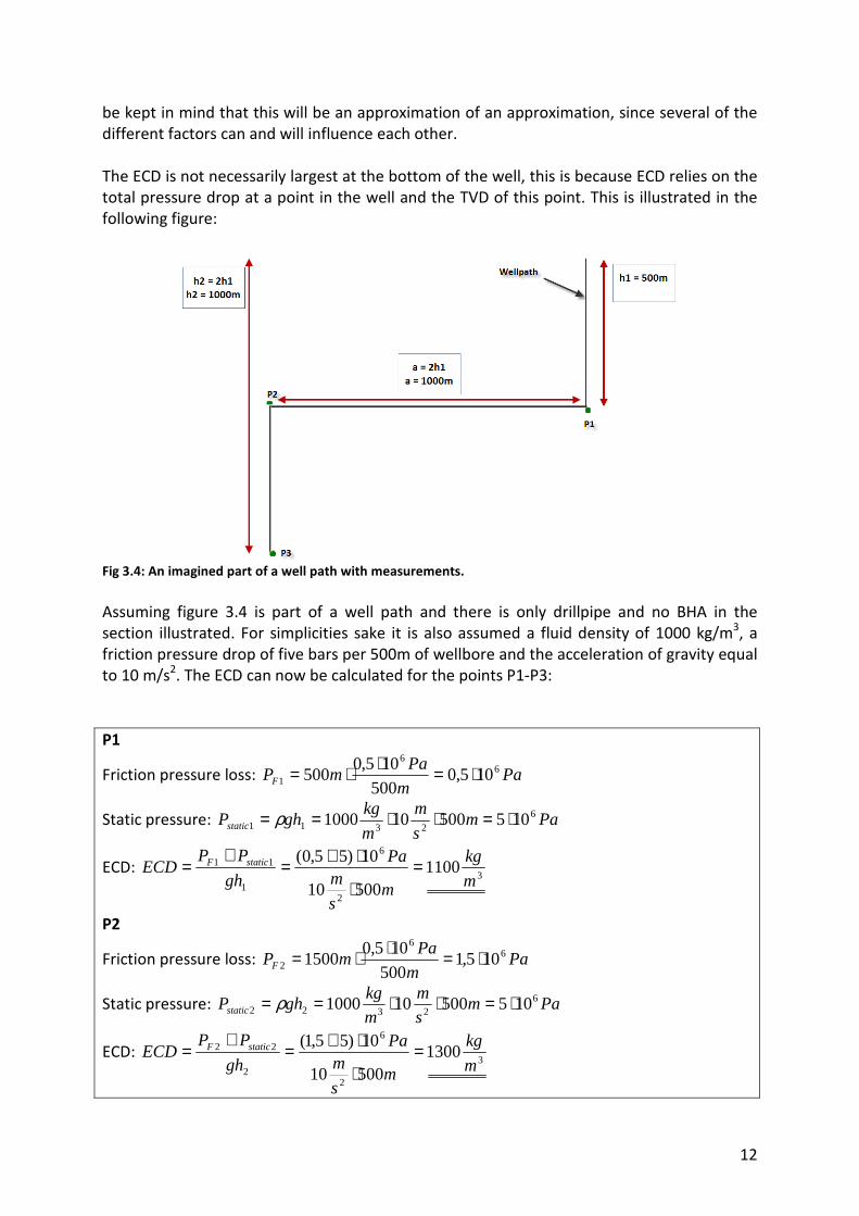
Fig 3.4: An imagined part of a well path with measurements.

Assuming figure 3.4 is part of a well path and there is only drillpipe and no BHA in the

section illustrated. For simplicities sake it is also assumed a fluid density of 1000 kg/m3, a

friction pressure drop of five bars per 500m of wellbore and the acceleration of gravity equal

to 10 m/s2. The ECD can now be calculated for the points P1-P3:

P1

Friction pressure loss: Pam

PamPF

66

1 105,0500

105,0500 ⋅=⋅⋅=

Static pressure: Pams

m

m

kgghPstatic

62311 105500101000 ⋅=⋅⋅== ρ

ECD: 3

2

6

1

11 110050010

10)55,0(

m

kg

ms

mPa

gh

PPECD staticF =

⋅

⋅+=+

=

P2

Friction pressure loss: Pam

PamPF

66

2 105,1500

105,01500 ⋅=⋅⋅=

Static pressure: Pams

m

m

kgghPstatic

62322 105500101000 ⋅=⋅⋅== ρ

ECD: 3

2

6

2

22 130050010

10)55,1(

m

kg

ms

mPa

gh

PPECD staticF =

⋅

⋅+=+

=

13

P3

Friction pressure loss: Pam

PamPF

66

3 102500

105,02000 ⋅=⋅⋅=

Static pressure: Pams

m

m

kgghPstatic

62333 10101000101000 ⋅=⋅⋅== ρ

ECD: 3

2

6

3

313 1200100010

10)102(

m

kg

ms

mPa

gh

PPECD staticF =

⋅

⋅+=+

=

Table 3.1: Calculations showing how the ECD in a well is dependent on the true vertical depth of the well.

The calculations show that the ECD is higher at P2 than any of the other two points. This

shows that the ECD is highly dependent on the well trajectory. As long as the well is being

drilled with a constant slope, the ECD will be highest at the bottom, but when the inclination

is changed the highest ECD will not necessarily be at the bottom. Regardless if the ECD is

higher at the bottom or not, the total pressure will always be highest at the bottom (if the

well deviation is at all depths equal to or less than 90 degrees). Due to this fact it is

favourable to have the measuring device for down hole pressure placed as close to the bit as

possible to get the most accurate ECD reading at this point.

3.5 Drilling in depleted zones

3.5.1 Heterogeneous depletion

Drilling in depleted zones can be very challenging. There are small margins between the PP

and fracture gradients. This means the pressure difference between static and dynamic

conditions in the well has to be small, which put strict limitations on the mud weight and

annulus pressure losses. The most challenging when drilling in depleted zones is, however,

that the formations being drilled through are not homogeneous. There can be zones of

significantly varying permeability. This means that when a reservoir is being produced, all

these zones experience different degrees of depletion. There will always be some kind of

communication between the zones for the pressure differences to even out through.

However, the time needed for this is often too long to accommodate the differences made

through years or decades of fluid extraction.

To illustrate this, and the effect on the drilling process, a simple diagram can be drawn, see

fig 3.2. Some assumptions are made; the PP is normal and 40% of σv, the density of the pore

water is 1,035 SG and the density of the rock formation is set to 1,035/0,4 = 2,5875 SG. Table

3.1 shows the estimated values thereof[2].

14

Formation Poison’s ratio PF percentage of σv Reduction of PF compared to

reduction of PP (%)

Salt 0,5 100,0 0,0

Shale 0,4 80,0 33,3

Sand stone 0,25 60,0 66,7

Chalk 0,15 50,6 82,4 Table 3.2: Fracture pressure in relations to the overburden, σv, and the reduction of fracture pressure in

relations to the reduction of pore pressure in different formation types, also called depletion factor in

chapter 4.1, underestimated depletion.

The same data is visualized in Fig 3.5.

Fig 3.5: PP and PF in a reservoir with different rock formations

[2].

The blue and green lines show PF and PP respectively, before fluid extraction. Red and purple

show the same after there have been fluid extraction in zones two and five. These zones

have had a reduction in PP which leads to a reduction in PF. The yellow areas shows the limits

the well pressure must be held within while drilling a horizontal well. The black line

represents a possible scenario of how the pressure in the wellbore would behave, with the

drill bit on the left side of this line.

As figure 3.2 shows it would be nearly impossible to drill in this example because of the low

PF in the produced chalk zone and the high PP in the unproduced zones. In Fig. 3.5 shale is

assumed to have the same pore pressure as the reservoir rocks. But shale often has a higher

PP than other formations like sand and chalk, because of its low permeability. If this is taken

into account it would be impossible to drill the shale section shown with conventional

drilling techniques without setting a casing or liner.

15

3.5.2 Managed Pressure Drilling

One way of solving the problem with small pressure margins is utilizing Managed Pressure

Drilling (MPD) technology. This is a methodology that has been developed and implemented

in the past years with great success to mitigate known and unknown drilling hazards[4]. By

creating a closed and pressurized mud returns system it is easier to predict and control the

reactions of the formation to the drilling program. The MPD systems can be divided into four

categories; HSE MPD, constant bottomhole pressure (CBHP) MPD, pressurized mud cap

drilling (PMCD) MPD and dual gradient MPD.

The main application of HSE MPD is to create a closed drilling fluid returns system to

minimize the risk of having human contact with hazardous material such as H2S or CO2, or if

a highly toxic drilling fluid system containing example caustics is used.

CBHP MPD is used in situations where a well is expected to experience kick-loss scenarios

when drilling in wells with close tolerance operation windows. The loss is characterized as

drilling fluid starting to flow into the formation when the mud pumps are started. This is

because the equivalent circulation density of the drilling fluid exceeds the formation

strength. If this is combated with a reduction in mud weight the pressure exerted by the

hydrostatic column might become insufficient to control the well in static conditions.

Formation fluid now starts to flow into the well which is the kick part. Applying a back

pressure to the circulating system allows for adjusting the bottomhole pressure (BHP) in the

well by reducing the back pressure under dynamic conditions, like when drilling, and

increasing it during connections, keeping a stable BHP at all time.

PMCD MPD is when drilling with a sacrificial fluid, i.e. no returns to surface. A light viscous

drilling fluid is also pumped down the annulus at a fixed rate with applied backpressure. The

drilling fluid pumped into the annulus is to keep the backpressure needed to control the well

to a minimum and at the same time prevent the sacrificial fluid to flow upwards. By doing

this the sacrificial drilling fluid along with cuttings and possible formation influx is forced

back into the weak parts of the formation which could be a drilling hazard.

Wells with a rapidly increasing pressure gradient cannot be drilled with a single drilling fluid

density without fracturing the overlying formation. This is the case, especially for deep water

wells. For conventional drilling this would be solved by setting a casing or liner and changing

the drilling fluid density. However, by use of a dual gradient MPD, this can be done without

the use of an intermittent casing. By injecting a lighter fluid into the annulus where the

pressure needs to be reduced, through a parasite string or through valves in the casing, a

heavier drilling fluid can be used below this point. This gives an increased pressure at the

bottom without the danger of fracturing the overlying formation.

3.6 Wellbore pressure

The pressure at the bottom of a well is governed by several different factors. The most

influential of these is the density of the drilling fluid used. By multiplying the density of the

fluid with the true vertical depth (TVD) of the well and the constant acceleration of gravity,

the static pressure of the well is given[5]:

16

ghP ρ= (15)

P = pressure (kPa)

ρ = density (kg/l)

h = depth of well (TVD)

g = constant acceleration of gravity (9,81 m/s2)

With no pumping, rotation of the drill string, or cuttings suspended in the drilling fluid, and

assuming that the density of the drilling fluid is constant throughout the wellbore, the above

equation gives the correct pressure seen at any depth in the wellbore.

3.6.1 Fluid friction

When the drilling process is started additional effects will contribute to increase the

wellbore pressure in the well. As drilling fluid starts to flow through the nozzles of the drill

bit and up through the annulus it starts to lose some of its energy, which is absorbed by

dissipation in friction forces. These friction forces are either due to internal friction in the

drilling fluid because of its viscosity, or external friction against casing and openhole walls[6].

This pressure loss due to the fluid flow is highly dependent on the rheological properties of

the drilling fluid and the velocities attained in the annulus. The pressure drop for a section of

annulus with a drillpipe inside can be calculated by the following[6].

Laminar flow:

3)()(63,408 ioio

FDDDD

LQP

−⋅+⋅=∆ µ

(16)

Turbulent flow:

38,1

2,08,18,0

)()(96,706 ioioF DDDD

QLP

−⋅+⋅=∆ µρ

(17)

ΔPF = pressure drop (kPa)

Q = volume rate (l/min)

Di = annulus inside diameter (in)

Do = annulus outside diameter (in)

ρ = drilling fluid density (kg/l)

μ = viscosity (cP)

L = measured depth of the section (m)

These equations give the pressure drop along an annulus with constant cross section. If

there is a change in the flow area the pressure drop for each section needs to be calculated

separately and then added together along the flow path[6]. These equations do not take

eccentricity into account and it is accordingly assumed that the drillpipe is in the center of

the wellbore throughout the whole section.

17

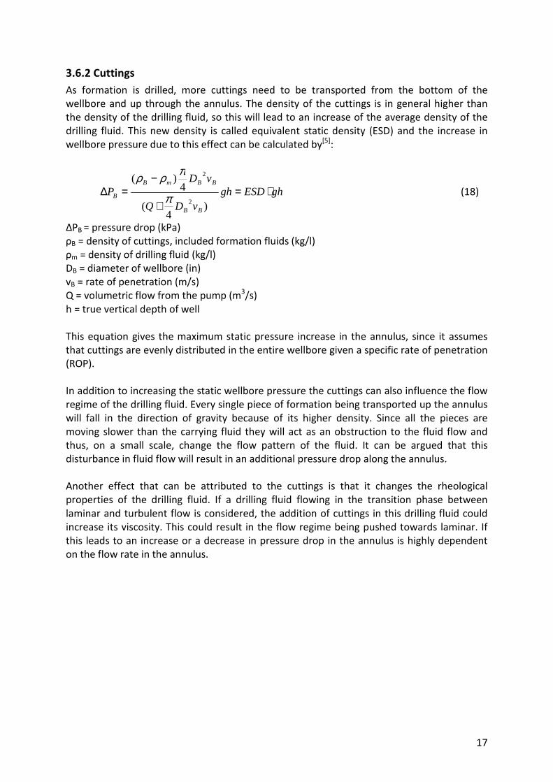
3.6.2 Cuttings

As formation is drilled, more cuttings need to be transported from the bottom of the

wellbore and up through the annulus. The density of the cuttings is in general higher than

the density of the drilling fluid, so this will lead to an increase of the average density of the

drilling fluid. This new density is called equivalent static density (ESD) and the increase in

wellbore pressure due to this effect can be calculated by[5]:

ghESDghvDQ

vDP

BB

BBmB

B ⋅=+

−=∆

)4

(

4)(

2

2

π

πρρ (18)

ΔPB = pressure drop (kPa)

ρB = density of cuttings, included formation fluids (kg/l)

ρm = density of drilling fluid (kg/l)

DB = diameter of wellbore (in)

vB = rate of penetration (m/s)

Q = volumetric flow from the pump (m3/s)

h = true vertical depth of well

This equation gives the maximum static pressure increase in the annulus, since it assumes

that cuttings are evenly distributed in the entire wellbore given a specific rate of penetration

(ROP).

In addition to increasing the static wellbore pressure the cuttings can also influence the flow

regime of the drilling fluid. Every single piece of formation being transported up the annulus

will fall in the direction of gravity because of its higher density. Since all the pieces are

moving slower than the carrying fluid they will act as an obstruction to the fluid flow and

thus, on a small scale, change the flow pattern of the fluid. It can be argued that this

disturbance in fluid flow will result in an additional pressure drop along the annulus.

Another effect that can be attributed to the cuttings is that it changes the rheological

properties of the drilling fluid. If a drilling fluid flowing in the transition phase between

laminar and turbulent flow is considered, the addition of cuttings in this drilling fluid could

increase its viscosity. This could result in the flow regime being pushed towards laminar. If

this leads to an increase or a decrease in pressure drop in the annulus is highly dependent

on the flow rate in the annulus.

18

Fig 3.6: A drawing showing how pressure drop in a fluid will behave with an increase in viscosity with regards

to flow rate.

The effect of changing from turbulent to laminar flow due to cuttings in the return drilling

fluid flow has not been documented and it is unknown if it would have any practical

application in drilling.

3.6.3 Drillstring rotation and eccentricity

The eccentricity of the drill string can influence the pressure drop in the annulus in a number

of ways. When considering all different annular geometries during a drilling operation, the

probability of a completely concentric annulus is very small at any given time[7]. An increase

in eccentricity, while not considering any other pressure influencing effects, will generally

lower the pressure loss over the eccentric interval. Although there is no change in the total

flow area of the annulus as the eccentricity increases, there will be an increase in the flow

area where the friction effect from the borehole wall and the outside of the drill string is

reduced. This allows the drilling fluid flow to become more stable.

Drill string rotation, like eccentricity, can influence the pressure drop in the annulus in a

number of ways. A drill string rotating in a concentric annulus with a fully developed laminar

flow does not influence the axial pressure drop for the section. This is because in laminar

flow the direction of the force in the flow is in one direction. By drawing the direction of the

flow as vectors it is more easily illustrated;

19

Fig 3.7: Figure showing the flow directions in a Newtonian flow with a non rotating drillpipe and a rotating

one.

Figure 3.7 shows a drillpipe being unfold to represent a sheet of metal. In the stationary

case, the flow direction (green arrow) will be straight up in axial direction. In the rotating

case the direction of the resultant flow (green arrow) will be shifted towards the direction of

the rotation. Since we can decompose the velocity as shown (green arrows), and friction

forces are proportional to the velocities for laminar flow, we see that the force in axial

direction is equal for the two cases FaR = Fa. The tangential, Fr, force only contributes to an

increase in torque on the drillpipe.

When eccentricity is applied the situation changes. Eccentricity alone will reduce the

pressure loss over a section, but when the drill string is rotating, the pressure loss over the

same section may increase if the rate of rotation is sufficiently large. This is due to inertial

forces caused by the rotation and eccentricity of the inner cylinder[8]. The magnitude of the

increase in pressure loss is a function of three dimensionless numbers, the Taylor number,

the eccentricity and a dimensionless gap width.

Fig 3.8: Annular space between inner- and outer cylinder, the displacement of the two circles centres is

shown with the letter e[8]

.

20

The eccentricity (ε) is defined as the centre of the inner tube’s deviation from concentric

placement divided by the difference of the two tubes radii, see Fig 3.8.

RR

e

−=

'ε (19)

ε = eccentricity

e = displacement of the inner cylinder

R’ =radius of the outer cylinder

R = radius of the inner cylinder

Fig 3.9: Dimensions of annular space

[8].

The dimensionless gap width (δ) is the distance from the inner tube to the outer tube,

divided by the radius of the inner tube as shown in Fig. 3.9.

R

d=δ (20)

δ = dimensionless gap width

d = distance from the inner to the outer cylinder (R’-R)

The Taylor number characterizes the importance of inertial forces due to rotation of a fluid

about a vertical axis relative to viscous forces. There are various definitions of the Taylor

number, which are not all equivalent, but the one used by G. Ooms and B. E. Kampman-

Reinhartz is[8]:

µρωRd

Ta = (21)

Ta = taylor number

ρ = drilling fluid density (kg/m3)

ω = rotational frequency of the inner cylinder (1/s)

The conditions investigated by G. Ooms and B. E. Kampman-Reinhartz[8, 9] only included

laminar flow of a Newtonian fluid. The pressure increasing effects are of course not limited

to these conditions, but for a turbulent regime and non-Newtonian fluids the flow

phenomena will become more complicated due to turbulence effects, shear rate and

viscosity variability.

21

As drilling commences, down hole conditions will change over time. The ROP might change,

the flow rate can change and drill string rotation is seldom constant. In addition the cuttings

will not behave the way we want them too. Ideally the cuttings should get transported

directly out of the annulus along with the drilling fluid, but this is not the case. Depending on

the inclination of the well the cuttings will form cutting beds, which will change depending

on several parameters. This calls for a method of predicting downhole conditions in a time

based model. S.S Costa et al[10] presented such a method that is capable of evaluating bed

height, cuttings concentration, pressure and ECD variations over the whole trajectory of the

well. By using mass and momentum conservation equations they were able to produce plots

giving a realistic description of the transient cuttings transportation in the wellbore. The

work was considered a first step in the development of a general tool to analyze complex

situations, which prediction of pressure and ECD in drilling conditions are.

3.6.4 Tool joints

Tool joints influence the pressure drop in the same manner as a change in wellbore diameter

does by changing the flow area. One way to calculate the effect of tool joints is to sum up

the total length of the joints and calculate the pressure drop over this “tool joint section” by

using Eq. (17). It is also important to subtract the length of all the tool joints from the rest of

the sections when calculating the rest of the pressure drop. If this method is used for

pressure drop calculation an important factor is not addressed properly. The Geometries of

the tool joints will have an effect on the flow of drilling fluid around them. Sharp angles and

edges will cause the fluid to undergo sudden contractions and expansions[11]. This results in a

significant loss of mechanic energy, compared to tapered tool joints, where the contraction

and expansion occurs more gradually.

When the fluid passes over the connections there is an increase in fluid velocity because of

the reduction in flow area. When the fluid has passed the connection the velocity is reduced

again. In a turbulent fluid flow, especially, the energy lost from the reduction in velocity is

used to make more vortices in the flow. This again shows that a section of connections

added up to represent one long stretch of pipe with a reduced flow area, will oversimplify

the calculation and give a lower pressure drop than what is observed.

3.6.5 Lateral drillstring movement

Lateral movement of the drill string in the wellbore is also a parameter that can affect the

pressure drop. A description of this lateral movement could be a drill string moving from one

side of the wellbore to the other and back again. As the drill string moves, drilling fluid in

front of the string is being displaced and fills the vacated area behind it. With the right

annular dimensions this lateral fluid velocity can be as high as five times the fluid velocity up

the annulus. Therefore the fluid can be in turbulent flow well below what is calculated as the

critical velocity of a stationary concentric annulus[7].

22

4. Case history - A loss of circulation incident in the North Sea

In 2006 a well in the North Sea experienced a major loss of circulation when drilling through

a depleted reservoir. The losses started shortly after drilling through a hard stringer and

were not cured until cement was squeezed into the loss zone. Investigation of the incident

did not reveal the true cause of the loss situation, but several interesting and plausible

explanations emerged.

4.1 Underestimated depletion

During the planning of the well the depletion of the reservoir being drilled through was

estimated to be around 80 bars. When calculating the reduction in the fracture pressure due

to this depletion a depletion factor is used. The depletion factor shows how much a

reduction in pore pressure will affect the fracture pressure. If the depletion factor is 0,50 it

means that a depletion in the pore pressure of 100 bar will give a reduction in fracture

pressure of 50 bar.

The first estimated depletion of 80 bars corresponds to a fracture pressure equal to 2,05 SG.

Back calculation after the loss, by using the mud weight in the system when the loss was

cured, showed a fracture pressure equal to 1,975 SG, corresponding to a depletion of as

much 160 bars. The calculation is done with a depletion factor of 0,67[12]. Using this value

shows that a depletion of 160 bars will give a reduction in the fracture pressure of about 107

bars.

It was also pointed out that this depletion calculation has errors, like uncertainties about the

mud weight and how the stress situation is in the formation and that the loss was due to the

depletion of the formation, so the answer could be even more, or less. Below in figure 4.1 is

a pressure curve plot made after the loss situation. It shows the pore pressure (black line),

mud weight (light green), ECD (green) and the fracture gradient (purple). Looking at this

could give the impression that underestimated depletion of the formation being drilled is the

main cause for the lost circulation. But having in mind the errors around the calculations, it

does not give a complete picture of the event.

23

Fig 4.1: Pressure curve plot showing PP, frac, MW and casing setting points. The values for the frac curve are

obtained from data collected after the loss occurred and is not the same curve as was on the pressure curve

plot made in the planning phase.

24

4.2 Shear tension in the formation

As mentioned in chapter 3.4, Drilling in depleted zones, the depletion of a formation is

seldom uniform. Often one part of the formation has a lower permeability and therefore has

had less formation fluid produced from it, leading to a higher pressure than, say, the more

permeable formation below. This difference in pressure in the two formations leads to shear

forces between them. The interface between the two formations now has tensions differing

from the normal σx, σy and σz described in chapter 3.1, Rock mechanics. These insitu forces

make the formation less resistant to outside influence, say, from the drill string and annulus

pressure.

When the drill bit now penetrates the hard stringer and goes into the softer formation

below, it is also drilling into an area with forces working in other directions than what they

were above. These areas, often below hard stringers or between formations with different

pressure regimes, is where drilling problems, like loss of circulation, occur more frequent

than when drilling in a formation where the distribution of forces is more homogeneous.

4.3 Pack off

In the following more specific details about the well in the North Sea

will be considered. The bottomhole assembly (BHA) used in the last

section of the well is shown in Fig. 4.2.

While drilling the last part of the 8 ½“ section the reported ROP was

20 meters per hour. About a meter before the loss occurred the ROP

dropped to 1-2. The pressure while drilling (PWD) measurement

device was located 5,2 meters above the bit, which is between the

GVR and EcoScope components in figure 4.2, and the memory dump

from this device showed no indication of an unnatural pressure

buildup, which means that a pack off must have happened below the

PWD. Since this is a short interval and very close to the bit there

would be no buildup of a cuttings bed, meaning all the cuttings

causing the pack off would have to come directly from newly drilled

formation. The most likely area for a pack off would be around the

GVR, a tool delivered by Schlumberger used to do logging while

drilling (LWD). The outside of the tool has a layout similar to a stab

making a potential area for cuttings to accumulate around.

When drilling through the hard section of formation there is a good

possibility the hole would be in gauge with the bit, with no sort of

washouts or hole abnormalities present. This would lead to a further

minimization of the flow area available around the GVR when it goes

through the stringer and the bit is drilling into the softer formation

below.

When the drill bit got through the hard stringer it is reported an

instantaneous increase in the ROP. How big this increase was at the

moment right after penetration is hard to say, mostly because the Fig 4.2: BHA drawing.

25

ROP measurement is averaged over time, but also because a correlation between ROP and

WOB is hard to get from the recorded data. This is because such a relation is also dependent

on parameters like drill string rotation rate and formation strength and type being known for

the interval in question. A good estimate of the ROP just after penetration of the stringer

could give an indication to the chances for a pack off due to increase in cuttings and

therefore volumetric flow around the GVR.

One way of telling if there was a pack off around the GVR would be to monitor the stand

pipe pressure. A peak in a pressure versus time plot would indicate such an incident taking

place. The timescale needed to see this peak would be at, or around, the one second

interval. The available data for the well was at a 10 second scale and did not show any

pressure peak. In addition to having a too long time interval for the measurements, the well

itself was 5172 meters MD when the loss occurred. There is a big possibility that the increase

of the standpipe pressure never would be recorded at the surface because of this long

distance and dampening effects in the drilling fluid system.

4.4 Stringer penetration

The shape of the drill bit can have an influence on how the hard stringer is being drilled

through. A bit with a round shape, like a sphere, would penetrate the hard section in the

middle before the edges has drilled through. A bit with more profile on the edges could have

the same effect on where the stringer is penetrated first, depending on the inclination of the

well path and the angle of the bedding plain.

Fig 4.3: Illustration of how different drill bit profiles would penetrate a formation. The red arrows point to

where the drill bit will first punch through.

Figure 4.3 is a concept drawing of two different drill bit profiles and how they would cut

through a section of hard formation. The inclination of the well and the angle of the hard

formation is arbitrary as similar illustrations can be obtained by changing the two. As one

part of the drill bit will penetrate the hard formation and reach the softer below, the rest of

26

the drill bit will continue to cut the stringer for some time, making it look like the whole

drilling assembly is hanging on an edge. Figure 4.4 below shows the low ROP, the green

circle and arrow, while drilling the stringer, and the increase seen after getting completely

through.

Having one part of the drill bit in contact with the softer formation below while the rest of

the stringer is being drilled can cause drilling fluid to be jetted into this zone. Depending on

how large the jet velocity is this could penetrate deep down, breaking up the formation and

cause a washout. This is only possible because the ROP while drilling the rest of the stringer

still is significantly lower than it would be drilling in softer sandstone. When the whole drill

bit is through the hard formation the broken up, softer formation would be drilled faster and

in larger pieces than expected. This could then easier lead to a pack off around the GVR tool.

If this jetting of drilling fluid into the formation below the stringer were to happen, it is

reasonable to assume that the drilling fluid would be lost in the soft formation. A look at the

drilling logs from the well shows, however that the drilling fluid return stay stable until the

major loss itself happens, indicating that jetting into the formation below while breaking

through the stringer did not contribute anything to the cause of the loss. See Fig. 4.4, red

circle.

Fig 4.4: A snapshot from the well log at the interval where the major loss occurs. No loss on the Active Tank

Volume Change (red circle to the right) is shown beforehand of the incident.

4.5 Drilling fluid properties

The drilling fluid used while drilling the 8 ½” section of the well was cesium format brine, a

drilling fluid used very seldom around the world. It was used for the first time world wide at

the Huldra field in the North Sea by Statoil ASA[13]. It does not contain any particles, not

counting lost circulation material (LCM) additives, since the weighting material is salt ions,

and it does not contain any base oil. This means it is not a good drilling fluid with respect to

creating a good mud filter cake in the wellbore. While drilling a good mud filter cake helps

prevent seepage losses of drilling fluid by plugging small cracks in the wellbore wall and by

plugging cracks it also helps preventing propagation of said cracks. This effect can prove to

be valuable when drilling into an already weak formation, or a potential loss zone, serving as

a preliminary strengthening agent.

27

The StatoilHydro guidelines for avoiding losses recommend to keep the fluid loss, which is an

indication of how much of the drilling fluid that escapes through the mud filter cake and into

the formation, lower than 2-3 ml / 30 min[14], and when drilling in high temperature high

pressure (HPHT) conditions below 1-2 ml / 30 min[15]. This was not done while drilling the

well in question. During previous sections of the well the fluid loss was, in fact, recorded to

be up to eight times higher than recommended.

Fig 4.5: Copy from a well report showing the fluid loss the last 100 meters of the 8 ½” section before the loss

occurred (red area)[16]

.

As figure 4.5 shows, the fluid loss for the last 100 meters vary between 5,8 and 10,8 ml / 30

min. This means that the starting point for avoiding or controlling loss situations, with

regards to the drilling fluid, is not as good as it could have been.

The cesium format brine used as drilling fluid had 40 kg of calcium carbonate solids per cubic

metre fluid, it was this mix that gave the before mentioned fluid loss of up to eight times as

high as the recommendation. To redeem this, another 100 kg of calcium carbonate and

graphite was added per cubic metre, which brought the fluid loss down to what is shown in

figure 4.5. The reason why no more solids were added was because the operators wanted

brine to flow into the formation. This influx could then be measured by the resistivity logging

tool, which in turn could be used to calculate the permeability of the formation being drilled.

The adding of solids was therefore a compromise between wanting to measure the

permeability and wanting to prevent loss of drilling fluids, and not an action taken solely to

prevent loss of circulation.

The main reason for choosing this unconventional drilling fluid system, which can be

compared more to a completion fluid than a standard drilling fluid, was because of its

stability. It is very resistant against sag, which is settling of particles, since there are almost

28

no particles in it, and it is a very stable system in a HPHT environment. In addition it yields a

lower ECD than oil based drilling fluids with similar densities do, and the dissolution of gas is

minimal[13].

Particles in a drilling fluid, as mentioned before, help to close up pores and cracks in the

formation. Depending on what kind of holes need clogging, different sizes of particles are

needed. As long as only the pore channels need to be clogged, small particle sizes are

sufficient. But if larger cracks, natural or drilling induced, are present, larger particles need to

be a part of the drilling fluid to more effectively plug the cracks.

While drilling the well there were used screens with 200 and 210 mesh during the entire 8

½” section. This is a fine mesh, filtering out the bigger particles in the already particle

deprived drilling fluid. To compensate for this, solids were added continuously during drilling

to try to maintain the wanted 140 kg / m3 solids concentration. What this basically means is

that the amount of large particles is kept constant, while the amount of smaller particles

increase since these pass through the mesh used on the shakers, and continue to circulate in

the system. Over time this will affect the d90 distribution of the particles. The d90

distribution is a measurement showing what particle size which 90 percent of the particles in

the drilling fluid are smaller than. The more small particles are present compared to large

particles, the lower the d90 particle size becomes.

During drilling the drill string will also act as a grinder on the particles in the drilling fluid.

Large particles will be crushed into smaller pieces on their way up the annulus because of

the mechanical movements of the drill string. This is another factor leading to the increase of

small particles in the drilling fluid. The lower the minimum particle size is in the d90

distribution, the smaller the chance larger particles will move into cracks in the formation

and aid in building a seal around them.

29

5. Discussion The loss of circulation incident could be a result of having underestimated the depletion of

the formation being drilled through, shear tensions in the formation due to heterogeneity in

the depletion, or a pack off. The reason discussed in chapter 4.1.4, “Stringer penetration”, is

not a likely reason since there was not observed any drop in the drilling fluid returns prior to

the loss incident, which happened after the stringer was drilled through.

If the reason for the loss was a pack off it would, as mentioned, have happened very fast and

just above the drill bit. This means there would have been very little time for the drill fluid to

chemically interact with the cuttings. In other words, if this were to be prevented something

would have to be done with the drilling parameters, adjusting them accordingly to the

situation. Since StatoilHydro already have well tested guidelines for stringer drilling[14], and

these were followed during the drilling operation, it is unlikely further optimization would

have a big impact on the success of drilling the stringer unless they were very drastic, which

could impede the efficiency of the operation.

The reason presented in chapter 4.1.5, Drilling fluid properties, is not a direct reason for the

loss occurring. It is more reasonable to categorize this as a reason for allowing the loss to

occur. The drilling fluid used is a very good fluid for drilling in a well known formation where

the problems can be anticipated or are known beforehand. When drilling into a depleted

formation, which was done in this case, where the depletion could be more serious than was

anticipated, the fluid is not optimal for handling a situation it is not designed for. Even thou

loss of circulation material (LCM) can be pumped into the well to try and cure a loss, it

should be evident that taking measures to minimize the risk for a loss happening is more

profitable than taking steps to redeem the situation afterwards.

Total E&P reports of drilling in a HPHT environment on Elgin/Franklin with a pressure

overbalance of 600 bars above the pore pressure and 100 bars over the estimated fracture

pressure[15]. The well they drilled was drilled with a conventional oil based drilling fluid, with

added solids specified to handle the conditions being drilled into. Similar cases can also be

found within StatoilHydro, Statfjord A reports drilling into a depleted formation with an ECD

overbalance of 44 bars as compared to the estimated fracture pressure; and Kristin reports a

successful drill run with an ECD overbalance of 80 bars.

These findings indicate that, either the estimated fracture pressures are not as accurate as

they are believed to be, or the drilling fluid used has certain properties that enhance the

wellbores resistance to loss of circulation incidents.

British Petroleum (BP) have a theory about wellbore strength they call “Stress Caging”. The

idea is that fractures are formed in the well and LCM material goes into these fractures and

plugs them. This causes the stresses around the borehole wall to keep it from fracturing at

other places. One way of illustrating this would be to drive a wedge shaped perfectly to fit a

crack into it. The wedge would prevent anything going into the crack, and the force exerted

from the wedge on the surrounding wall would increase the walls resistance to cracks

forming other places. Although this theory explains why an ECD well above the fracture

pressure is observed, it could just as well be a good drilling fluid filter cake preventing the

30

cracks to form. By blocking small cracks and pore openings the drilling fluid is prevented

from flowing into these and causing the formation to fracture any further.

The d90 distribution of particles needs to be held at a level where the probability of the

larger particles getting into cracks and plugging them is high enough to minimize the risk of a

loss of circulation incident, at least when conventional drilling techniques are being used.

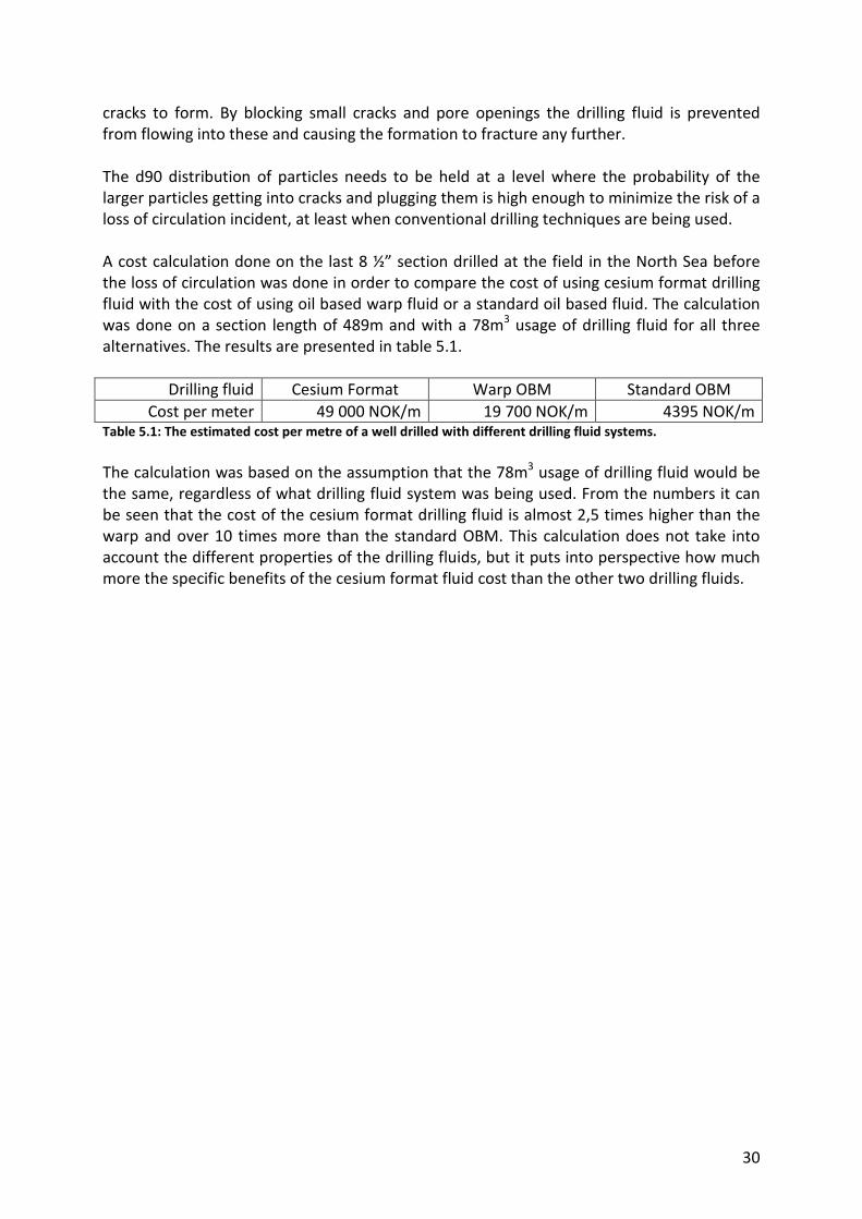
A cost calculation done on the last 8 ½” section drilled at the field in the North Sea before

the loss of circulation was done in order to compare the cost of using cesium format drilling

fluid with the cost of using oil based warp fluid or a standard oil based fluid. The calculation

was done on a section length of 489m and with a 78m3 usage of drilling fluid for all three

alternatives. The results are presented in table 5.1.

Drilling fluid Cesium Format Warp OBM Standard OBM

Cost per meter 49 000 NOK/m 19 700 NOK/m 4395 NOK/m Table 5.1: The estimated cost per metre of a well drilled with different drilling fluid systems.

The calculation was based on the assumption that the 78m3 usage of drilling fluid would be

the same, regardless of what drilling fluid system was being used. From the numbers it can

be seen that the cost of the cesium format drilling fluid is almost 2,5 times higher than the

warp and over 10 times more than the standard OBM. This calculation does not take into

account the different properties of the drilling fluids, but it puts into perspective how much

more the specific benefits of the cesium format fluid cost than the other two drilling fluids.

31

6. Conclusion During drilling of new wells problems can occur that were not anticipated from the start, or

the source of the problem can be very hard to pinpoint because of uncertainty or lack of

measurements.

In the case discussed here in this thesis the problem that happened was loss of circulation.

Even though the cause of this incident cannot be determined with absolute certainty, a lot of

the data collected point toward an underestimation of the depletion in the formation, which

causes stresses that cannot be directly controlled when drilling conventionally. Even though

the drilling fluid used is a good drilling fluid for HTHP conditions, it is not flexible enough to

cover conditions it is not specifically designed for.

Based on the case presented in this thesis, it is recommended not using this type of drilling

fluid system as a standalone solution in conventional drilling. Utilizing another drilling fluid

with more particles in addition to follow guideline procedures set from other experiences,

would help minimize the chances for this type of drilling hazard to happen again. If one

wishes to use the cesium format drilling fluid because of the properties it has that more

conventional systems lack, steps have to be taken so that the benefits of a convention

drilling fluid also applies to the cesium format system. This can be achieved either by adding

enough solids to the fluid so that a good drilling fluid filter cake will be made down hole, or

by utilizing MPD technologies, which take away the need for such a drilling fluid filter cake.

32

7. References

1. Fjær, E., et al., Petroleum Related Rock Mechanics. Vol. 2nd. 2008, Amsterdam:

Elsevier.

2. Skaugen, E., Boring med liner i lavtrykksreservoar. 2009.

3. Harrison, H.G. EQUIVALENT CIRCULATION DENSITY 2007 07.01.2007 [cited 2009

24.03.2009]; Available from: http://www.peteng.com/jmm/ecd01.html.

4. Grayson, B., Increased Operational Safety and Efficiency With Managed Pressure

Drilling. 2009.

5. Skaugen, E., Kompendium 1 Boring. 1997, Stavanger: HiS.

6. Gabolde, G. and J. Nguyen, Drilling Data Handbook. 8th ed. 2006, Paris: Editions

TECHNIP.

7. Marken, C.D., X. He, and A. Saasen, The Influence of Drilling Conditions on Annular

Pressure Losses. SPE, 1992.

8. Ooms, G. and B.E. Kampman-Reinhartz, Influence of drillpipe rotation and eccentricity

on pressure drop over borehole during drilling. European Journal of Mechanics,

B/Fluids, 1996. 15(5): p. 695-711.

9. Ooms, G. and B.E. Kampman-Reinhartz, Influence of Drillpipe Rotation and

Eccentricity on Pressure Drop Over Borehole With Newtonian Liquid During Drilling.

SPE, 2000. 15(4): p. 249-253.

10. Costa, S.S., et al., Simulation of Transient Cuttings Transportation and ECD in

Wellbore Drilling. SPE, 2008.

11. Simones, S., et al., The Effect of Tool Joints on ECD While Drilling. SPE, 2007.

12. Undertun, O., Written communication. 2009.

13. Saasen, A., et al., Drilling HT/HP Wells Using a Cesium Formate Based Drilling Fluid.

SPE, 2002: p. 6.

14. StatoilHydro, Quick Reference Guide Best Practice Drilling Operations. 2008. 47.

15. Singelstad, A.V. and T.H. Omland, Verbal and written communication. 2009.

16. Baroid Fluid Services - End of well report. 2006.