3

SAND98-8203Unlimited Release

Printed November 1997

DRFM: A N EW PACKAGE FOR THE EVALUATION

OF GAS-PHASE TRANSPORT PROPERTIES.

Phillip H. Paul, 8351Sandia National Laboratories

Livermore CA

Abstract This report describes a complete and modernized procedure to evaluate purespecies, binary and mixture transport properties of gases in the low density limit. Thisincludes a description of the relationships used to calculate these quantities and the meansused to obtain the necessary input data. The purpose of this work is to rectify certainlimitations of previous transport packages, specifically: to employ collision integralssuitable for high temperatures, to modernize the mixture formula, and to modernize theinput data base. This report includes a set of input parameters for: the species involved inH2 -, CO - air combustion, the noble gases, methane and the oxides of nitrogen.

4

Acknowledgment This work was supported by The United States Department ofEnergy, Office of Basis Energy Sciences, Chemical Sciences Division. The author isindebted to Dr. J. L. Durant Jr. of Sandia National Laboratories who performed the SCFcalculations and to Prof. Dr. J. Warnatz of Ruprecht-Karls-Universität Heidelberg wholent his considerable expertise and support to these studies.

5

DRFM: A N EW PACKAGE FOR THE EVALUATION

OF GAS-PHASE TRANSPORT PROPERTIES.

Phillip H. Paul, 8351Sandia National Laboratories

Livermore CA

Introduction This work is directed at updating the current transport packages (e.g.MIXRUN [1], CHEMKIN’s TRANLIB [2] and EGLIB[3]) as used for calculation of thetransport properties of pure species and mixtures. This work grew out of a growingawareness that the previous package gave predicted values that were well outside of theacceptable range of tolerable error. The result of this work is a complete replacement ofthe old packages. The new package incorporates a number of advances including a morephysically realistic molecular potential as based on the recent works of Mason and co-workers, a modernized data base including a self consistent set of parameters for radicalspecies (albeit some are calculated but at least none are guessed), and a modernization ofthe means of computing mixture properties as based on the recent works of Ern andGiovangigli [4]. The current transport package in CHEMKIN was released in 1986 and islargely based on the works of Mason and co-workers (early 60’s), the basic structureemployed and much of the data base comes from the works of Warnatz [1,5]. This wasand remains a solid tool for gas-phase simulations and by its existence has provided oneof the fundamental supports for research into reacting flows.

A test was performed by using the existing CHEMKIN package to predict pure speciesviscosity and thermal conductivity and equimolar thermal diffusion factors, for stablespecies, as functions of temperature. The results were then compared to the valuestabulated by Bzowski et al. [6] and by Uribe et al. [7]. In general the predicted thermalconductivity compared poorly (for some of the stable species deviations exceeded 20%).Predictions for viscosity were somewhat better with the worst case being H2 which waspredicted 15% low of the experimental value at 2000K when compared to the datatabulated by Assael et al. [8]. The predictions for the thermal diffusion factor were quitepoor with differences exceeding 100% for mixtures with disparate molecular weights.

The following presents a complete and updated set of procedures for the calculation ofpure species and mixture transport properties, including: thermal conductivity, binarydiffusivity, thermal diffusion factor and shear viscosity. These procedures have beenimplemented in a new transport code (named DRFM for ‘dipole reduced formalism’)which as of this writing has little resemblance to existing transport packages and is thusnot (repeat not) plug compatible with application programs that employ these packages.This is due in part to the need to transfer more information between the preprocessor and

6

the actual property functions used in the application codes, and the desire to make thenew transport code suitable for use with parallelized codes.

Collision Integrals The transport properties are expressed in terms of the collisionintegrals Ωij

(1,1)* and Ωij(2,2)* and the higher order functionals Aij* , Bij* , Cij* and Eij*

which are functions of temperature and normalized molecular parameters for the collisionpartners (here indicated by the subscripts). In the previous implementations (e.g.MIXRUN, CHEMKIN’s TRANLIB and EGLIB) the collision integrals were developedfrom a Stockmeyer 12-6-3 potential which reduces to the more common Lenard-Jones 12-6 potential for all but polar-polar molecule interactions. One of the input parameters forevery pure species is the Lenard-Jones (LJ) well depth, ε, which is an energy usuallyexpressed in Kelvins. As part of the calculation of transport properties it is necessary toemploy a set of combination rules which provide the well depth (and other molecularparameters) for non-identical collision partners. The simplest combination rule for welldepth gives ε ε εij i j≈ . More accurate combination rules are given below. It is well

known that the LJ inverse 12th power repulsive component becomes to stiff or hard forkBT > 10ε. An exponential repulsive component is required to accurately calculatetransport properties at higher collision energies hence at higher temperatures. This isparticularly important for combustion applications in which case species with relativelysmall well depths, like H and H2, are important at high temperatures. For H, H2 and N2

the well depths are of order 5, 25 and 98 K, respectively. Thus an exponential repulsivepotential is required to accurately calculate diffusion of H into N2 or viscosity of pure H2for temperatures above of order 250 K. It is completely possible to apply the LJ-basedcollision integrals for kBT > 10ε however this amounts to a curve fit in which casemolecular parameters obtained, by fitting H2 viscosity data (say), cannot be used beyondthe curve fit. Formally, parameters obtained outside the range of valid application of thepotential cannot be subsequently used in accordance with the principle of correspondingstates to derive binary diffusion coefficients or mixture properties.

Following the prescription of Bzowski et al. [6] the collision integrals in the new packageare broken into two ranges, a Lenard-Jones 12-6 for kBT < 10ε and an exponentialrepulsive for kBT > 10ε. Polynomial expression for the collision integrals are given byBzowski et al. [6] which are appropriately spliced together over the full range oftemperatures. These polynomials (reproduced here in Appendix F for completeness) havebeen analytically combined to obtain the higher order collision functions. The non polar-polar collision integrals are thus functions of three molecular parameters (in CHEMKINthey are a function of a single parameter, the reduced temperature T* = kBT/ε), being T*and the normalized energy V* = V/ε and radius ρ*= ρ/σ for the exponential potential. Itis important to note that the relations used in the new package, as given by Bzowski et al.[6], apply for T* greater than unity. They make this restriction in that at lower reducedtemperatures quantum effects become important. They do provide expressions forcollision integrals for the noble gases applicable for T* < 1.

Quantum effects Quantum effects become important when the size parameter, σ,approaches the de Broglie wavelength. In kinetic theory it is common practice to define areduced deBoer parameter

7

( )Λ ij

ij ij B ij

h

m k

* =σ ε

1 2 (1)

which is the ratio of the de Broglie wavelength to the size parameter for a kinetic energyequal to the well depth. The gas behaves classically at all temperatures in the limit thatΛij* goes to zero. Whereas quantum effects becomes significant for large values of Λij* asTij* gets small. For example, quantum effects can be safely ignored for Ne-Ar mixtures(Λ* = 0.34, ε = 64K) for temperatures above 30K or T* > ½, whereas quantum effectsbecome important for 3He-4He mixtures (Λ* = 2.81, ε = 10.4K) for temperatures below20 to 30 K or T* = 2 to 3. At present there is no consistent means of treating the collisionintegrals for other than the noble gases below T* = 1.

In the new package we have introduced polynomial extensions of the representations forthe classical collision integrals covering the range 0.2 ≤ T* < 1.0 which are analytic tosecond order with the representations given by Bzowski et al [6] through T* = 1. This isdone to be able to call into the code and get an appropriate values for species like H2O(Λ* = 0.2, ε = 535K) at ambient temperature.

Exponential repulsive potentials, a case in point: Normal Hydrogen Assael et al. [8]applied LJ based collision integrals to fit H2 viscosity data over the range 20 < T <2200K, to find εH2 = 33.3 K and σH2 = 2.968Å. However their fit shows strong systematicdepartures from the measurements at both low and high temperatures. Whereas restrictingthe fit to 1≤T*≤10 we find εH2 = 23.957 K and σH2 = 3.063Å. From these parameters andthe potential of Partridge et al. [9] we obtain ρH2* = 0.103 and VH2* = 1.14x105. With thisnew parameter set, the deviations in the calculated values are less than the scatter in theexperimental data over the entire range of temperatures.

Exponential repulsive potentials, a case in point: Atomic Hydrogen To obtain inputdata for atomic hydrogen, Dixon-Lewis [10] made use of the LJ radius estimated bySvehla [11] σH = 2.07 Å, and applied LJ based collision integrals to fit the diffusioncoefficient measured by Clifford et al. [12] (i.e. DH-N2 = 1.35 ± 0.3 cm2/s at one atm. and300K) to find εH = 37.0K. The well depth was revised upward in CHEMKIN to a value ofεH = 145.0K (the result of assuming σH = 2.07 Å and fitting to H-H2 data at 300K). Wangand Law [13] have observed that these input data for H atom are not consistent withresults obtained from other experiments and calculations, and have suggested values ofσH = 3.52 Å and εH = 9.1 K. In using these new values they calculated (again usingtransport properties based on LJ collision integrals) a net reduction in laminar flamesspeeds for H2-air mixtures as compared to those predicted using the original parametervalues in the CHEMKIN transport data base. This decrease in flame speed is a directresult of the modified parameters for H atom which yield a decrease in H atom diffusionrates.

Using recent beam data and more complete combination rules (than those employed byWang and Law [13] ) we find values of σH = 3.288 Å and εH = 5.417 K which if appliedin the same fashion as Wang and Law [13] would yield a further a further reduction in the

8

H atom diffusion rates and hence a further reduction in the predicted flame speeds.However the ab initio calculations of transport properties by Stallcop et al. [14] for H-N2

mixtures and by Clark and McCourt [15] for H-H2 mixtures suggest quite the opposite,the H atom diffusion rates should be higher than predicted by CHEMKIN. The root ofthis discrepancy is the inadequacy of the LJ based collision cross sections to predicttransport properties for T > 10ε . Binary diffusion coefficients as calculated usingcollision integrals derived from an exponential repulsive potential and using inputparameters obtained solely from beam data, are found to be in good agreement with thepredictions of the ab initio calculations and with the reported diffusion coefficientsmeasured for H into H2, N2 and Ar at 300K.

Polar-Polar Collision Integrals The existing transport libraries employ a Stockmeyerpotential specifically to handle polar-polar interactions. Essentially all of the molecularcombustion radicals are strongly polar as is water. It is interesting to note that in theCHEMKIN data base only water, methanol, ammonia and CH3O are given as polar. As aresult of having left most the dipole moment entries at zero, the use of this same data basewith the more simple 12-6 potential would have achieved essentially the same result asthe 12-6-3 potential with much less computational effort.

The Stockmeyer potential is not isotropic (i.e. it depends on relative molecularorientation) and is written in the form

( ) ( )( ) ( )ϕ ω εσ

ξ ζ ωσ

δ ζ ωσ

ij ij d id ij ij d d ijrr r r

, * *=

− +

−

− −4 1

12 6 3

(2)

where the ζ(ω) represent the relative angle dependence in the dipole-induced dipole (d-id)and dipole-dipole (d-d) attractive terms. Monchick and Mason [16] evaluated collisionintegrals for all possible orientations and then by geometrically averaging the results overall angles obtained a new set of collision integrals as a function of two reducedparameters; T* = T/ε and δ* = µ2/2εσ3. There was a great deal of discussion in theliterature regarding the theoretical basis for this approach but the method has survived inessence because it appeared to work reasonably well for viscosity and binary diffusion ofpolar species. This approach could be extended to include the exponential repulsivepotential, however this would require a massive tabulation of collision integrals asfunctions of 5 dimensionless parameters.

A number of simplifying alternatives to the formalism of Monchick and Mason [16] havebeen attempted. One is to take the values of ζd-d(ω) and ζd-id(ω) as constants. Another isto use a thermally orientation-averaged potential of the form

( )( ) ( )( )

( )( )ϕϕ ω ϕ ω ω

ϕ ω ωr

r r k T d

r k T d

B

B

=−

−∫∫∫

∫∫∫, exp ,

exp ,(3a)

This ‘central’ or ‘spherical’ potential can be expanded in a series which leaves to loworder

9

( )ϕ εσ σ

ξγ ε δ

ij ij

ij ij

ij

ij ijr

r r T=

−

+ +

4 1

2

3

12 6

*

*2

(3b)

Formally the expansion provides a value of γ = 1. These alternatives turned out to workpoorly because they strongly under- and over-estimated the dipole-dipole contributions.Similar results were observed by Singh and Das Gupta [17] who evaluated the viability ofa like series expanded central potential for evaluating transport properties for collisionpairs subject to strong dipole-quadrapole interactions.

Gray and Gubbins [18] observe that the low order terms in an expansion for an effectivecentral potential should match those in an expansion for the thermodynamic propertiesand the centers pair correlation function of a system actually having a pure centralpotential. Taking this into account requires a value of ¼ ≤ γ ≤ ½ which has the effect ofmediating the strength of the dipole-dipole term. We have tested the ability of thisformalism to fit experimental viscosity data for some 20 strongly polar molecules andfind excellent results for a fixed value of γ = ¼ . The LJ parameters recovered from thenew fits for species with δ∗ less than of order unity are in reasonable agreement withthose recovered by re-fitting the same data with a Stockmeyer potential. In every casetested the quality of the new fits (as evidenced by the residuals and confidence intervalsfor the fit parameters) were superior using the effective central potential with γ = ¼ thanthose obtained using the Stockmeyer potential. It is interesting to note that in applying theStockmeyer potential, Monchick and Mason [16] did not report fits for molecules havingvalues of δ∗ greater than of order unity. The Stockmeyer fits for δ∗ greater than unity arefound to be poor (for reference δ∗ = 2.1, 2.1, 2, 1.6, 1.2, and 0.7 for CH3F, HCN, CH3CN,HF, H2O, and NH3 , respectively). In contrast the fits using the effective central potentialwith γ = ¼ work uniformly well for all of the polar species tested (over the range 0.03 <δ* < 2.4).

The important advantage gained in using the effective central potential is that the dipole-dipole and dipole-induced dipole terms can be incorporated directly into the collisionintegrals for non polar-polar interactions by defining effective LJ and exponentialrepulsive parameters. First, define the quantity

χα µ α µ

ε σiji j j i

ij ij

≡+2 2

64(4a)

which is dimensionless and is zero only if both species are non-polar. Then define

∆ ij

i j

ij ij

≡µ µ

ε σ

2 2

624(4b)

which has units of energy (e.g. Kelvin) and is zero unless both species are polar. Then theeffective parameters become

10

( )′ = + +ε ε χij ij ij ij T12

∆ (5a)

( )′ = + +−

σ σ χij ij ij ij T11 6

∆ (5b)

( )′ = + +−

V V Tij ij ij ij* 1

2

χ ∆ (5c)

( )′ = + +ρ ρ χij ij ij ij T* 11 6

∆ (5d)

As such the transport property calculation is in terms of 6 reduced parameters for everycollision pair: εij , σij , V* ij , ρ* ij , χij and ∆ij .

Combination Rules The new transport data base includes 7 molecular parameters foreach pure species. There are:

ε Lenard-Jones well depth (K)

σ Lenard-Jones radius (Å)

V* ≡ V/ε exponential (Born-Mayer) potential energy

ρ* ≡ ρ/σ exponential (Born-Mayer) potential radius

α molecular static polarizability (Å3)

µ molecular dipole moment (Debye)

C6* ≡ C6/εσ6 normalized dispersion energy

A data base containing sets of parameters for a number of the species of interest incombustion and aerothermodynamic flows is given in Appendix B.

Following the prescriptions of Bzowski et al., [6,19] and Tang and Toennies [20] themolecular parameters are combined according to the following rules:

1) Let ai = σi(1- (C6,i* /2.2)1/6) for all C6,i* < 2.2 and ai = 0 otherwise

2) Determine σij = (σi + σj )/2

3) Let

XC

Ciji

j

j

i

=

α

α6

6

1 2

,

,

(6a)

11

and then determine

( ) ( )( )( )

ε ε εσ σ

σij i j

i i j j

ij i jij ij

a a

a a X X=

− −

− +

+

3 3

6

2

2

1(6b)

4) Determine

ρρ σ ρ σ

σiji i j j

ij

** *

=+

2(6c)

5) Finally determine

VV V

ijij

ij

i

i

i

ijj

j

j

ij* =

ρε ρ ρ

ρρ

ρρ2 2

(6d)

Note that in these combination rules, the ‘ * ‘ superscript refers to normalized quantitieswhereas the absence of this superscript refers to a dimensioned quantity (e.g. ρ = ρ* σ orC6 = C6* ε σ6 ). Bzowski et al. [6,19] give a more sophisticated combination rule for σij

but the correction appears as less than 1% and is thus ignored here.

Binary Diffusion The binary diffusion coefficients, Dij, are given by

nDk T

m

dij

B

ij

ij

ij ij

=+3

8 2

12 1 1π σ Ω ( , )* (7)

here mij ≡ mimj/(mi+mj) and n is the total number density. The higher order correction isin terms of the factor dij which depends on the mixture composition and has the form

( )d Cc

c cij iji

i i

= −− +

13 6 51

2. * α

αβ(8a)

where ci = xi/(xi +xj) and

( )α =

+

2

8 1 182

1 1

2 2.

( , )*

( , )*m mj i

ij

ii

Ω

Ω(8b)

( )β = + +

10 1 18 3

2. m m m mj i j i (8c)

The convention for evaluation of dij is to re-order i and j such that mj ≤ mi (note that thisreordering is only for the computation of dij and as such the Dij remain symmetric underexchange of i and j).

12

For the self diffusion coefficient (i.e. the case of i = j ) the correction is obtained by takingci = 1 and mi = mj. The higher order correction is in general small being most importantfor the diffusion of a trace light species into a heavy partner. For a trace heavy or a traceslightly heavy species (e.g. xi << xj and mj << mi or mj ≈ mi, respectively) then dij goes tozero. In contrast, for a trace slightly light or a trace light species (e.g. xj << xi and mj ≈ mi

or mj << mi, respectively) then dij ≈ 1.3(6Cij* -5)/58 or dij ≈ 1.3(6Cij* -5)/10,respectively. The later case may amount to as much as a 10 percent increase in the binarydiffusion coefficient.

Shear Viscosity The pure component shear viscosity is given by

ηπ σi

i B i

ii ii

m k T h=

+5

16

12 2 2Ω ( , )* (9a)

with the correction term

( )h Ei ii= −3

1968 7

2* (9b)

To calculate mixture viscosity (discussed below) it is necessary to define a fictitiousbinary viscosity of the form

ηπ σij

ij B

ij ij

m k T= 5

16

12 2 2Ω ( , )* (10)

Thermal Conductivity Prior methods for calculating pure species thermal conductivity,λ, have been based upon: 1) kinetic theory which predicts that λ is closely related to theshear viscosity, and 2) the works of Eucken [21] who suggested that the persistence oftransitional energy did not hold for energy carried by the molecular internal degrees offreedom, and thus that external and internal degrees of freedom could be treatedseparately. With these assumptions

mc f cv tran

λη

= +5

2 , int int (11)

where cv = cv,tran + cint is the heat capacity of the molecule, and fint is the persistence-length ratio for internal energy. The common expressions for fint are based on a first ordertheory which contains a number of approximations and omissions, such as the neglect ofspin polarization, ‘complex’ collisions and certain correlations between internal energystates and relative transitional energy. With these simplifications the expression for λ andthe mixture formulas contain a number of inelastic cross sections and relaxation timesthat are poorly or completely unknown.

Uribe et. al. [7] have proposed a correlation for pure species thermal conductivity andhave applied it successfully to calculations for N2, CO, CO2, O2, NO, CH4, CF4 and SF6.They note that the correlation cannot be applied to species like C2H4 and C2H6 which

13

have multiple coupled internal modes, beyond rotation, that can be excited in thermalcollisions. A consideration of each internal mode requires a separate diffusion factor anda correction for mode-mode coupling. They observe that modes with long lifetimes can beconsidered independent (e.g. τvib >> τrot in linear diatomic molecules). In NO anelectronic mode is active but contributes only a small fraction to Cp and τelec > 10τrot, thustreating this mode as independent provides a reasonable approximation. The correlationfor λ proposed by Uribe et. al. [7] requires as input: 1) a knowledge of η(T), Dii(T) andCp(T); 2) molecular dipole and quadrapole moments; 3) molecular rotational constants; 4)LJ well depth; 5) a rotational collision number, Zrot, at some temperature; and, 6) a spin-polarization parameter. They achieve reasonable success in predicting λ for HCl but notethat the expression used for Zrot(T) is based on a theory for homonuclear diatomics andthus may not extend well to polar species.

The previous means of calculating pure component thermal conductivity rely on the firstapproximation for the diffusion coefficient and ignore or use simple models for inelasticexchange and spin collisions. Exchange collisions being particularly important for polarmolecules (e.g. for HCl, a 15 % error in predicted thermal conductivity at 300 K isincurred without explicit consideration of exchange collisions). Some transport packagesdo include an ad hoc but somewhat hidden correction for exchange effects in polar-polarcollisions for particular species. It has become apparent that there is no general means tocalculate thermal conductivity of pure species even given much more input data thansupplied in the previous or new data bases. However both CHEMKIN and EGLIB requirethe capability to calculate thermal conductivity in order to calculate the multicomponentthermal conductivity of a mixture.

Hirschfelder et al. [22] give a relation for the thermal conductivity of a multicomponentmixture of monatomic gases in terms of a four-block L matrix. Subsequently Monchick,Pereira and Mason [23] extended this definition to employ a 9-block L matrix as a meansof incorporating polyatomic species. This Monchick, Pereira and Mason formalism wasadopted by Dixon-Lewis [10] and is the means employed to calculate multicomponentthermal conductivity in CHEMKIN and in EGLIB. The additional components of the 9-block L-matrix have an explicit dependence on the specific heats and diffusioncoefficients of molecular internal modes, inelastic cross sections and relaxation timeswhich describe both the pure species thermal conductivities and the interactions withunlike collision partners.

Muckenfuss and Curtiss [24] observed that the conductivity of a mixture of monatomicspecies as given by the 4-block L-matrix was obtained by mixing terms in the first andsecond approximation. They find a considerably simpler representation (solely in terms ofthe L11 block) for mixture thermal conductivity as a consequence of carrying theexpansion to completion in the second approximation. Hirschfelder et al. [22, see notesadded in 2nd printing] recommended adopting this representation. Hirschfelder [25]further recommended that the thermal conductivity of a multicomponent mixturecontaining polyatomic gases be expressed as a linear sum of the thermal conductivity ofthe mixture as if all the components were monatomic and the thermal conductivity due tointernal degrees of freedom, in what is termed the Hirschfelder-Eucken formalism.

14

Uribe et al. [26] invoke three recent developments to obtain a predictive algorithm formixture thermal conductivity:

1) The use of experimental or accurately calculated values for the pure species transportproperties and dropping all other explicit dependencies on inelastic cross sections.This is in essence a return to the Hirschfelder-Eucken formalism. The diffusioncoefficients for internal energy are replaced by ratios of ordinary mass diffusioncoefficients. The use of this interpolation scheme corrects most of the deficiencies inthe first order theory except for mixtures in which the masses of the components arevery different.

2) Najafi et al. [27] investigated the properties of mixtures of noble gases. They suggestthat the problem with disparate mass ratios can be largely corrected by using theproper diffusion coefficient rather than its first approximation.

3) Reliance on accurate data for binary diffusion coefficients, pure component viscosityand thermal conductivity.

Based on these, Uribe et al. [26] give a working formula for a mixture of N components

λ λλ

ληmix mix

m i

im

B

ii i

i

N

i jii

ijj i

Nk

mx x x

D

D= + −

+

= = ≠

−

∑ ∑( )( )

,

115

41 1

1

(12)

which is the relation proposed by Hirschfelder [25]. Here the xi are the mole fractions ofthe constituents and the superscript (m) refers to a hypothetical thermal conductivity as ifthe molecule behaved like a monatomic gas, that is

λ ηim

B i ik m( ) ≡ 15 4 (13)

One result of using equation 12 for the mixture thermal conductivity is that it is no longernecessary to be able to decompose the pure species thermal conductivity into internal andexternal components for the purpose of calculating mixture properties. In the newpackage, the only requirement for pure species thermal conductivity is of the form

Pi i im≡ λ λ( ) (14)

We have adopted the procedure of supplying the function Pi(T) in the form of apolynomial curve fit as a part of the transport data base (see Appendix A). This data canbe obtained by fitting to experimental data or to accurate calculations performed off-line,or in a pinch by assuming some simplified relation for the Prandtl number (see appendixA). Two of the input parameters required in the existing CHEMKIN transport data base,Zrot and LIN, are thus no longer required having been replaced by the input curve fit forPi.

Thermal Diffusion Factors The binary thermal diffusion factor, αTij , contains acomplicated dependence on composition, molecular mass and collision integrals. It isuseful to define a reduced thermal diffusion factor, αR, via

15

α αTij Riji j

i j i j

x S x S

x Q x Q x x Q≡

−

+ +

1 22

12

2 12

(15)

where the functionals S and Q depend on collision integrals and the molecular masses ofboth species (the expression for these functions are given by Bzowski et al. [6] and arereproduced in Appendix E for completeness). In equation 15 the terms containing the Sand Q carry the major dependencies on composition, molecular mass and the collisionintegrals that represent the interactions of like molecules. The reduced factor can beapproximated by

( )( )α κRij ij TijC≈ − +6 5 1* (16)

The quantity κT is described as small and is generally neglected in calculations [6]. Theapproximation for the reduced diffusion factor is then the difference between twonumbers of similar magnitude and demonstrates the extreme sensitivity in αT to effectsthat occur in the interaction of unlike molecules. That the thermal diffusion factor is asecond order transport property is best seen via the relation given by Marreno and Mason[28]

( )( )α

∂∂R ij

ij

P

D

T,

( )ln

ln≅ −

4 2

1

(17)

where Dij(1) represents the binary diffusion coefficient in the first approximation. As a

result of this sensitivity, Bzowski et al. [6] find that calculated values of αT may involveuncertainties that are an order of magnitude greater than the uncertainties in calculatedvalues for viscosity or binary diffusion coefficients. They also note that errors in theexperimental data for the thermal diffusion factor involve uncertainties of similarmagnitude.

Unlike the other transport properties the thermal diffuison factor retains a strongdependence on both composition and temperature and thus must be evaluated ‘on-line’ ina reacting flow simulation. Paul and Warnatz [29] have expanded the thermal diffusionfactor for large values of the ratio mi/mj and give a simplified relationship suitable for usein reacting flow simulation codes (see Appendix D).

Calculation of Mixture Properties The calculation of multicomponent diffusioncoefficients (i.e. Di,j

(m) the binary diffusion coefficient of the i’th and j’th species pairwithin a multicomponent mixture) requires the solution of a constrained, possiblysingular, set of linear equations. As of this writing, only mixture-averaged diffusioncoefficients are implemented in the new package, given by

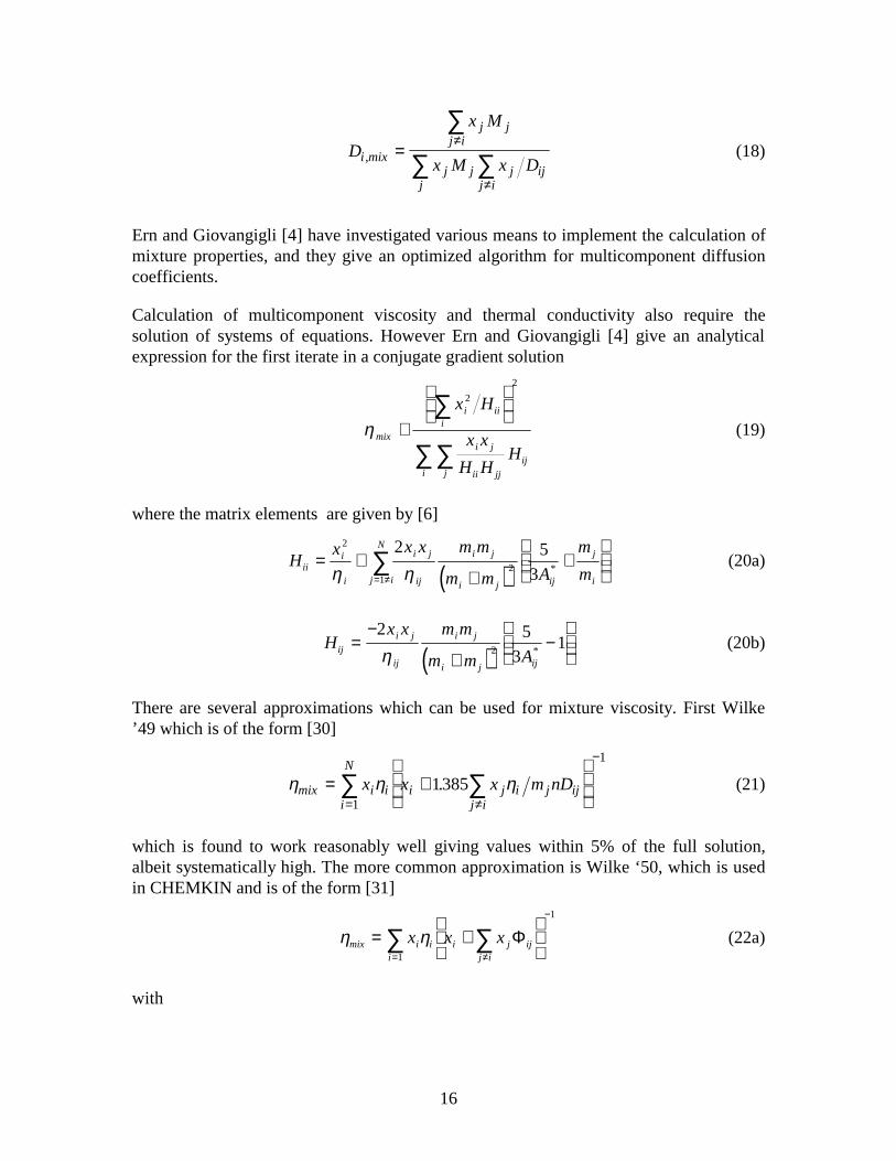
16

D

x M

x M x Di mix

j jj i

j jj

j ijj i

, =≠

≠

∑

∑ ∑ (18)

Ern and Giovangigli [4] have investigated various means to implement the calculation ofmixture properties, and they give an optimized algorithm for multicomponent diffusioncoefficients.

Calculation of multicomponent viscosity and thermal conductivity also require thesolution of systems of equations. However Ern and Giovangigli [4] give an analyticalexpression for the first iterate in a conjugate gradient solution

ηmix

i iii

i j

ii jjij

ji

x H

x x

H HH

≅

∑

∑∑

2

2

(19)

where the matrix elements are given by [6]

( )H

x x x m m

m m A

m

miii

i

i j

ij

i j

i j ij

j

ij i

N

= ++

+

= ≠∑

2

21

2 5

3η η * (20a)

( )H

x x m m

m m Aiji j

ij

i j

i j ij

=−

+−

2 5

312η * (20b)

There are several approximations which can be used for mixture viscosity. First Wilke’49 which is of the form [30]

η η ηmix i i i j i j ijj ii

N

x x x m nD= +

≠

−

=∑∑ 1385

1

1

. (21)

which is found to work reasonably well giving values within 5% of the full solution,albeit systematically high. The more common approximation is Wilke ‘50, which is usedin CHEMKIN and is of the form [31]

η ηmix i i i j ijj ii

x x x= +

≠

−

=∑∑ Φ

1

1

(22a)

with

17

Φ ijj

i

i

j

i

j

m

m

m

m= +

+

−

1 8 11 4 1 2 2 1 2

ηη

(22b)

This relation has been found to work as well as Wilke ’49.

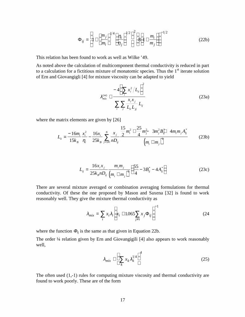
As noted above the calculation of multicomponent thermal conductivity is reduced in partto a calculation for a fictitious mixture of monatomic species. Thus the 1st iterate solutionof Ern and Giovangigli [4] for mixture viscosity can be adapted to yield

λmixm

i iii

i j

ii jjij

ji

x L

x x

L LL

( ) ≅−

∑

∑∑

4 2

2

(23a)

where the matrix elements are given by [26]

( )L

m

k

x x

k

x

nD

m m m B m m A

m mii

i

B

i

i

i

B

j

ij

i j j ij i j ij

i jj i

N

=−

−+ − +

+= ≠∑16

15

16

25

15

2

25

43 42

2 2 2

21η

* *

(23b)

( )L

x x

k nD

m m

m mB Aij

i j

B ij

i j

i j

ij ij=+

− −

16

25

55

43 42

* * (23c)

There are several mixture averaged or combination averaging formulations for thermalconductivity. Of these the one proposed by Mason and Saxena [32] is found to workreasonably well. They give the mixture thermal conductivity as

λ λmix i i i j ijj ii

x x x= +

≠

−

∑∑ 1065

1

. Φ (24

where the function Φij is the same as that given in Equation 22b.

The order ¼ relation given by Ern and Giovangigili [4] also appears to work reasonablywell,

λ λmix k kk

x≅

∑ 1 4

4

(25)

The often used (1,-1) rules for computing mixture viscosity and thermal conductivity arefound to work poorly. These are of the form

18

λ λ λmix j jj

j jj

x x= +

∑ ∑

−1

2

1

2

1

(26)

a similar (-1,1) relation can be written for ηmix.

While it is possible to calculate full multicomponent thermal diffusion coefficients usingthe methods given by Hirschfelder et al. [22] or by Ern and Giovangigli [4], thecomplexity and extra computational load may not be warranted given the inherentuncertainties in the thermal diffusion factors. Chapman and Cowling [33] give themixture-averaged thermal diffusion ratio of the i’th species into the mixture as

k x xTi i k ikk

N

==

∑ α1

(27)

where the sum of the kTi over the mixture is identically zero.

Input Data Base The data base for each pure species is composed of two parts; 1) a setof seven parameters to describe the molecular potential, and 2) a fit for the ratio λ / λ(m) .Also required are the molecular weights. Note that the specific heats, which are requiredin the previous packages, are not required in the new package.

Bzowski et al. [6] report full parameter sets for N2, O2, NO, CO, CO2, CH4, CF4, SF6 andthe noble gases. They also give a partial parameter set (lacking V* and ρ* ) for C2H4 andC2H6. The beam data summarized by Tang & Toonies [20] has been used to provide a fullparameter set for H. The beam data of Aquilanti et al. [34] has been similarly used toextract a full parameter set for O. A full parameter set for N was obtained from the beamdata of Pirani and co-workers [35] and the ab initio potentials employed by Stallcop et al.[36]. A full set of parameters for H2 was obtained by fitting viscosity data as tabulatedand referenced by Assael et al.[8] and from the ab inito potentials given by Partridge etal. [9].

For almost any stable species and for a number of the combustion radicals, values for thepolarizability and dipole moment can be found in the literature. To some extent values forC6 are also available. Such information is available for a number of strongly polarmolecules including H2O, NH3, NO2, HCN, SO2, OCS, H2S, C2H5OH, CH3OH,(CH3)2CO, (CH3)2O, HBr, HCl, HF, CH3CN and many fluoro-chloro-carbons. Theavailable experimental viscosity data for all of these polar species has be refit using thenew potential described above (where necessary, the data has been selected to limit thefits to 1 ≤ kBT/ε ≤ 10). Given ε, σ, α, µ and C6* a consistent set of V* and ρ* parametershas been obtained using the prescriptions of Tang and Toonies [37]. Their methodrequires higher order dispersion parameters which were obtained using the correlationsC8* = (4/3)C6* (α/σ3)1/3 and C10* = (5/4) C8*

2/C6*. This leaves a large number of speciesof interest for which there is no experimental transport data (e.g. OH, CH3, CH2O) and agood number of these for which even the polarizability and dipole moments are unknown.

19

We have performed a self-consistent fields (SCF) simulation using GAUSSIAN ‘92 [38]for the full set of species included in GRImech 2.1 [39] which includes the standard set ofspecies considered in C(1) and C(2) hydrocarbon combustion chemistry as well as a set ofspecies associated with NOx formation. The purpose of the simulation was to obtaindipole moments and polarizabilities for the entire set. Species with known values werecarried as a test of the SCF simulation. Values for ε, σ and C6* were then calculated,given a polarizability and an equivalent oscillator number, following the prescriptions ofCambi et al. [40] Again species with known values were carried as a test. Finally valuesfor V* and ρ* were calculated as described above and species with known values werecarried as a test.

The data used for the polynomial fits for the ratio λ / λ(m) were obtained from a numberof sources including: For H2O the data for viscosity and thermal conductivity were takenfrom the compilation by Matsunaga and Nagashima [41]. For H2 the data for viscosityand thermal conductivity were taken from the compilation of Assael et al. [8]. For manyof the stable non-polar species the data was obtained from the tabulations of Bzowski etal. [6] and Uribe et al. [7] which were supplemented by the studies by Wakeman and co-workers [42]. Additional data was taken from the compilations by Beaton and Hewitt [43]and Touloukian and co-workers [44]. Fits for OH and H2O2 are based on the applicationof the correlation model of Uribe et al. [7].

Additions to the Data Base For the parameter set: The preferable means is to begin bygetting polarizability and dipole moment data from the literature, followed by fittingexperimental viscosity data, restricted to 1 < T* < 10, to obtain the LJ parameters. Thendetermine a value for C6* from the fit parameters and a literature value for C6. Finally,since beam data for the repulsive parameters or high temperature viscosity data to fit therepulsive parameters are very scare, obtain V* and ρ* using the procedure describedabove. In the absence of any experimental data then the starting point must be an SCFcalculation for the polarizablity and dipole moment, and C6 if possible. Followed by thefull procedures outlined above.

For the polynomial fits: For a monatomic species the answer is unity. For molecules againthe best place to start is the literature. Failing this a high quality calculation can be used,of the form described by Uribe et al. [7]. For stable species a literature search iswarranted. There is an extensive line of new studies into the properties of pure specieswhich follow the works of Wakeham and co-workers [42]. These studies fit experimentaltransport data to what are termed Thijssen cross sections (which are denoted by a symbollike ϑ ) which are related to but not the same as the transport cross sections describedabove.

Accuracy It is useful to consider the accuracy of the transport properties as predicted bythe new package. The best predictions are for the properties of N2, O2, NO, CO, CO2,CH4, CF4, SF6 and the noble gases as based on the parameter sets, collision integrals andcombination rules, given by Bzowski et al. [6]. They estimate accuracies of 1% for ηmix,5% for Dij and 25% for the thermal diffusion factor. For the viscosity of pure H2 theparameter set used in the new package gives values within 2% of the mean from 50 to

20

2200 K which is within the scatter in the experimental data. For the stable polar species,the fits for pure species viscosity are all within the experimental scatter which is less than5% of the mean. For H-Ar, H-N2, H-H2, O-N2 and O-Ar mixtures at 300 K, the predictedbinary diffusion coefficients are within the experimental error bars, which are of order25%.

For thermal conductivity, Uribe et al. [7] estimate an accuracy of 1.5% for 300-500K and3% for lower/higher temperatures for N2, CO, CO2, N2O, CH4, CF4 and SF6. For O2 andNO they estimate accuracies of 3% for 300-500K and 5% for lower/higher temperatures

Summary and Caveat Emptor A complete and updated algorithm for calculating purespecies and mixture transport properties has been described. The procedures used toobtain from the literature or to estimate the required input data (where not available in theliterature) have also been described. The input data base will evolve as betterexperimental data becomes available and as the capability of SCF calculations evolves toprovide better predictions of molecular parameters. To quote the CHEMKIN transportmanual, with reference to the new data base, ‘This data base should not be viewed as thelast word in transport properties. Instead, it is a good starting point from which the userwill provide the best available data for his particular application.’ Having said this auseful lesson can be learned through an examination of a collection of CHEMKINtransport data bases as obtained from sources around the world. These reveal that theoriginal data base parameters remain largely unchanged. These data bases appear to havebeen modified but only to introduce new species. In which case the new parameters werelargely obtained by copying those for some other species that was thought to be ‘similar’.The are a number of examples of entries for silicon, sulfur and gallium bearingcompounds with non-physical LJ well depths in excess of several thousands of Kelvins.Finally there is one entry for something with the name ‘E’ which is listed as a monatomicspecies with a LJ well depth of 850 K and a radius of 425.0 Å. Whatever it is, ‘E’ iscertainly not any known atomic species and is simply too large to be a sub-atomic particle(also charged particles like electrons are completely outside of the realm of validity of thetransport model), possibly an antibody.

One is left with a philosophical question: If the inclusion of terms for the Soret andDufort effects are essential to accurately model flames and CVD processes (as somebelieve) and these effects are related to derivatives of diffusion coefficients, then, is itimportant to get the diffusion coefficients right? If so then this requires accurate inputdata, use of an appropriate potential and the possible use of higher order approximationsto the transport properties. Otherwise, for reacting flow computations, it may be betterand even closer to the correct answer to simply drop Soret and Dufort and even assumemixture properties equal to- and binary diffusion into-the largest component. The currentwork is an effort to address these issues. One must assume that given another 10 years orless this new package will be found lacking and need to be replaced.

Future Developments The only plans (by the author) for further work on this packageare: 1) the refinement and testing of the development code and the application of thiscode to particular flow calculations as a means of investigating the impact of changes inthe computation of the transport properties; and 2) the completion of the data base to

21

include species relevant in C1 and C2 hydrocarbon-air and NOx chemistry as well as anumber of other stable species of interest. As of this writing and as noted in theintroduction, there are no formal plans in place to make this work a plug-compatiblereplacement for existing transport codes.

22

References

1) J. Warnatz, Ber Bunsenges. Phys. Chem. 82, 193-200 (1978). J. Warnatz, BerBunsenges. Phys. Chem. 82, 643-649 (1978). J. Warnatz, in The 18th Symposium(International) on Combustion (the Combustion Inst. Pitts. PA, 1981), pp369-384.

2) R. J. Kee, G. Dixon-Lewis, J. Warnatz, M. E. Coltrin and J. A. Miller, A FORTRANcomputer code package for the evaluation of gas-phase multicomponent transportproperties, (Sandia National Laboratories, 1986), report SAND86-8246.

3) A. Ern and V. Giovangigli, EGLIB: A General Purpose FORTRAN Library forMulticomponent Transport Property Evaluation, (software manual, 1996).

4) A. Ern and V. Giovangigli, Multicomponent Transport Algorithms (Springer-Verlag,NY, 1994). A. Ern and V. Giovangigli, J. Comp. Phys 120, 105-116 (1995).

5) J. Warnatz, ‘Influence of transport models and boundary conditions of flamestructure,’ in Numerical Methods in Flame Propagation, N. Peters and J. Warnatzeds. (Friedr. Viewag and Sohn, Wiesbaden, 1982).

6) J. Bzowski, J. Kestin, E. A. Mason and F. J. Uribe, J. Phys. Chem. Ref. Data 19,1179-1232 (1990). J. Bzowski, J. Kestin, E. A. Mason and F. J. Uribe, ‘Equilibriumand transport properties of gas mixtures at low density: eleven polyatomic gases andfive noble gases,’ (AIP Aux. Pub. service, NY) document JPCRD-19-1179-98.

7) F. J. Uribe, E. A. Mason and J. Kestin, Physica A 156, 467-491 (1989). F. J. Uribe, E.A. Mason and J. Kestin, J. Phys. Chem. Ref. Data 19, 1123-1136 (1990).

8) G. J. Assael, S. Mixafendi and W. A. Wakeham, J. Phys. Chem. Ref. Data 15, 1315-1322 (1986).

9) A. Eucken, Z. Physik 14, 324-329 (1913).

10) J. O. Hirschfelder, C. F. Curtiss and R. B. Bird, Molecular Theory of Gases andLiquids, 2nd ed. (Wiley, NY, 1964).

11) L. Monchick, A. N. G. Pereira and E. A. Mason, J. Chem. Phys. 42, 3241-3256.

12) G. Dixon-Lewis, ‘Computer modeling of combustion reactions in flowing systemswith transport,’ in Combustion Chemistry, W. C. Gardiner ed. (Springer-Verlag, NY,1984).

13) C. Muckenfuss and C. F. Curtiss, J. Chem. Phys. 29, 1273-1277 (1958).

14) J. O. Hirschfelder, in The 6th Symposium (International) on Combustion, (Reinhold,NY, 1957), pp. 351-366.

15) F. J. Uribe, E. E. Mason and J. Kestin, Int. J. Thermophys. 12, 43-51 (1991).

16) B. Najafi, E. A. Mason and J. Kestin, Physica A 119, 387-391 (1983).

17) T. R. Marrero and E. A. Mason, J. Phys. Chem Ref. Data 1, 3-118 (1972).

18) P. H. Paul and J. Warnatz, ‘A re-evaluation of the means used to calculate transportproperties of reacting flows,’ (in preparation, 1997).

23

19) C. R. Wilke, J. Chem. Phys. 18, 517-521 (1950).

20) J. W. Buddenberg and C. R. Wilke, Ind. Chem. Eng. 41, 1345 (1949).

21) E. A. Mason and S. C. Saxena, Phys. Fluids 5, 361-369 (1958).

22) S. Chapman and T. G. Cowling, The Mathematical Theory of Non-uniform Gases,(Cambridge U. Press, 1970).

23) H. Partridge, C. W. Bauschlicher, J. R. Stallcop and E. Levin, J. Chem. Phys. 99,5951-5960 (1993).

24) R. A. Svehla, ‘Estimated viscosities and thermal conductivities of gases at hightemperatures,’ (NASA, 1962), NASA Tech. Report R-132.

25) A. A. Clifford, P. Gray, R. S. Mason and J. I. Waddicor, Proc. R. Soc. Lond. A 380,241-258 (1982).

26) H. Wang and C. K. Law, ‘Diffusion coefficients of hydrogen atom for combustionmodeling’, presented at and in proceeding of, The Fall 1996 Meeting of the EasternStates Section of the Combustion Inst., at Hilton Head NC, Dec 1996, paper 110.

27) J. R. Stallcop, H. Partridge, S. P. Walch and E. Levin, J. Chem. Phys. 97, 3431-3436(1992).

28) G. B. Clark and F. R. W. McCourt, Chem. Phys. Let. 236, 229-234 (1995).

29) L. Monchick and E. A. Mason, J. Chem. Phys. 55, 1676-1697 (1961).

30) Y. Singh and A. Das Gupta, J. Chem. Phys. 52, 3055-3063 (1970). Y. Singh and A.Das Gupta, J. Chem. Phys. 52, 3064-3067 (1970).

31) C. G. Gray and K. E. Gubbins, The Theory of Molecular Fluids, (Clarendon, Oxford,1984).

32) J. Bzowski, E. A. Mason and J. Kestin, Int. J. Thermophys. 9, 131-143 (1988).

33) K. T. Tang and J. P. Toennies, J. Phys. D 1, 91-101 (1986).

34) V. Aquilanti, R. Candori and F. Pirani, J. Chem. Phys. 89, 6157-6141 (1988).

35) G. Liuti, E. Luzzatti, F. Pirani and G. G. Volpi, Chem. Phys. Let. 121, 559-563(1985). B. Brunetti, G. Liutti, E. Luzzatti, F. Pirani and G. G. Volpi, J. Chem. Phys.79, 273-277 (1983).

36) J. R. Stallcop, C. W. Bauschlicher, H. Partridge, S. R. Langhoff and E. Levin, J.Chem. Phys. 97, 5578-5585 (1992).

37) K. T. Tang and J. P. Toennies, J. Chem. Phys. 80, 3726-3741 (1984).

38) M. J. Frisch, GAUSSIAN 92 Rev. B. (Gaussian Inc. Pittsburg PA, 1992).

39) M. Frenklach, H. Wang, M. Goldenberg, G. Smith, D. Golden, C. Bowman, R.Hanson, W. Gardiner and V. Lissianski, (Gas Research Inst., 1995), Topical ReportGRI-95/0058.

24

40) R. Cambi, D. Cappelletti, G. Liuti and F. Pirani, J. Chem. Phys. 95, 1852-1861(1991).

41) N. Matsunaga and A. Nagashima, J. Phys. Chem. 87, 5268-5279 (1983).

42) V. Vesovic, W. A. Wakeham, G. A. Olchowy, J. V. Seugers, J. T. R. Watson and J.Millat, J. Phys. Chem. Ref. Data 19, 763-808 (1990). J. Millat and W. A. Wakeham,J. Phys. Chem. Ref. Data 18, 565-581 (1989). A. Fenghour, W. A. Wakeham, V.Vesovic, J. T. R. Watson, J. Millat and E. Vogel, J. Phys. Chem. Ref. Data 24, 1649-1667 (1995).

43) Physical Property Data for the Design Engineer, C. F. Beaton and G. F. Hewitt ed.s,(Hemisphere, NY 1992).

44) Thermal Conductivity, Y. S. Touloukian and C. Y. Ho ed.s (IFI/Plenum, NY, 1970).Viscosity, Y. S. Touloukian and C. Y. Ho ed.s (IFI/Plenum, NY, 1975).

25

Appendix A: Thermal Conductivity Data Base

The polynomial representing the ratio λ/λ(m) has the form

( )P TC C y C y

C y C y C y=

+ ++ + +

1 3 52

2 42

631

(A1)

where y ≡ ln(T) with T in Kelvins. The exact form of this polynomial was selected as themost compact form which adequately fit all the data for the species considered, and whichdisplayed reasonable high and low temperature behavior outside of the range of availabledata. Coefficients are given in Table A1 as restricted to 250 K < T.

Table A1: Fit coefficient for the polynomial Pi

C1 C2 C3 C4 C5 C6

CH4 1.0124190 -.35704300 -.31147680 .04240417 .02568945 -.00160871

CO 0.9133026 -.3384788 -.26450910 .03584491 .01961665 -.00108565

CO2 1.5518010 -.2911856 -.54380010 .02452900 .05427209 0.0

H2 0.6123433 -.4207392 -.20620020 .05689904 .01770746 -.00238307

H2O 0.5931511 -.1095666 -.03359944 0.0 0.0 0.0

H2O2 0.0243916 -.2087738 0.07258789 .01300192 0.0 0.0

HO2 -0.422988 -.1763043 0.16050169 0.0113138 0.0 0.0

O2 0.7759023 -.3787674 -.23802530 .04579047 .01837284 -.00170918

OH 0.7319990 -.3669068 -.21580729 .04311154 .01598934 -.00157644

NO 0.9576946 -.3496382 -.28842830 .03810040 .02220485 -.00117394

NO2 3.6188066 -.1954056 -.65721492 0.0 0.0 0.0

N2O 1.6153915 -.2973629 -.55752424 .02503407 .05408830 0.0

N2 1.0367960 -.3182594 -.29313580 .03122558 .02160071 -.00079964

Monatomic species (e.g. H, O, N, He, Ne, Ar, Kr and Xe) have the value, P ≡ 1.0.

26

Hirschfelder [1] gives a simple relation for the Prandtl number in terms of the Euckenfactor

( ) ( )( )Pr . .int≅ + −−

C R f C RP P375 251

(A2)

and gives a value of fint = 1.27 for non-polar species. Which then gives

PC

R

f C

Rp P≡ ≅ + −

4

15

11

2

3

2

51

Print (A3)

This type of expression can be used to constrain the behavior at high temperatures.

Recent studies by van den Oord and Korving [2] and by Wakeman and co-workers [3]have employed the set of collision integrals developed by Thijsse et al. [4] to quantify thevarious elastic and inelastic cross sections involved in transport processes. They havebegun the process of re-evaluating single species transport data in terms of the Thijssecross sections. Recently Schreiber et al. [5] have detailed expressions for mixtureproperties in terms of the Thijse cross sections. However at the present time, there isinadequate cross section data to implement these new relationships.

Van den Oord and Korving [2] give a remarkably simple correlation for the Prandtlnumber given by which is applicable in the limit that the collision numbers for relaxationof internal modes are ordered such that Zelec, Zvib >> Zrot, then

( )Pr *≅ +

2

31

4

3π Z T

c

Rrot

rot (A4)

In the limit that T* is of order or greater than unity, the rotational internal energy hasreached a high temperature limiting behavior in which case crot/R ≈ 1 and 3/2 for linearand nonlinear molecules, respectively. The temperature dependence in the rotationalcollision number can be expressed in terms of the correlation [6,3]

( )Z T ZT T Trot rot

** * *= + +

++

∞

−

12

2 4

2

3 2

1 2

2 3 2

3 2

1π π π

(A5)

Thus the high temperature behavior of the Prandtl number can be estimated in terms ofthe species specific constant Zrot

∞ (here the superscript refers to a temperature). Note thatthe previous CHEMKIN transport package required as input (to be used in thermalconductivity calculations) the parameter Zrot

300 which is directly related to Zrot∞ by this

correlation given a value for the LJ well depth, ε. Values for Zrot∞ can be obtained from

the literature, or by analysis of experimental thermal conductivity data [e.g. 1,3,6], orpossibly from spectroscopic measurements of rotational relaxation rates. This correlationalso provides a means to constrain the high temperature range of the fits to physicallymeaningful values.

In terms of Thijssen cross sections the Prandtl number is given by [2]

27

Pr = ϑ10E / ϑ20 = 2/3 (1 + ϑ0010 / 2ϑ20 ) (A6)

where ϑ0010 is an inelastic cross section describing the collision-induced interchangebetween translation and internal modes. The quantity Zrot = 4 ϑ20 / πϑϑ0001 where ϑ0001 is across section for rotationally inelastic effects. Thus

Pr = (2/3)(1 + 2ϑ0010 / (πϑϑ0001 Zrot)) (A7)

In the limit that Zrot << Zvib, Zelec then ϑ0010 / ϑ0001 = 2crot/3kB , which then yields equationA4 above.

References

1) J. O. Hirschfelder, in The 6th Symposium (International) on Combustion, (Reinhold,NY, 1957), pp. 351-366.

2) R. J. van den Oord and J. Korving, J. Chem. Phys. 89, 4333-4338 (1988).

3) V. Vesovic, W. A. Wakeham, G. A. Olchowy, J. V. Seugers, J. T. R. Watson and J.Millat, J. Phys. Chem. Ref. Data 19, 763-808 (1990). J. Millat and W. A. Wakeham,J. Phys. Chem. Ref. Data 18, 565-581 (1989). A. Fenghour, W. A. Wakeham, V.Vesovic, J. T. R. Watson, J. Millat and E. Vogel, J. Phys. Chem. Ref. Data 24, 1649-1667 (1995).

4) B. J. Thijsse, G. W. ‘tHooft, D. A. Coombe, H. F. P. Knaap and J. J. M. Beebakker,Physica A 98, 307-314 (1979).

5) M. Schreiber, V. Vesovic and W. A. Wakeham, Int. J. Thermophys. 18, 925-938,(1997).

6) F. J. Uribe, E. A. Mason and J. Kestin, Physica A 156, 467-491 (1989). F. J. Uribe, E.A. Mason and J. Kestin, J. Phys. Chem. Ref. Data 19, 1123-1136 (1990).

28

Appendix B: Molecular Potential Data Base

Table B1: Molecular potential parameters

species ε (K) σ (A) µ (Debye) α (A3) V* ρ* C6*

CH4 161.40 3.721 0 2.60 3.07E06 0.0698 2.100

CO 98.40 3.652 0.1098 1.95 5.31E04 0.1080 2.630

CO2 245.30 3.769 0 2.65 2.80E06 0.0720 1.860

H 5.42 3.288 0 0.667 3.70E04 0.1010 6.586

H2 23.96 3.063 0 0.803 1.14E05 0.1030 4.245

H2O 535.21 2.673 1.847 1.450 3.50E07 0.0640 1.612

H2O2 368.11 3.499 1.573 2.230 8.23E05 0.0830 2.322

HO2 365.56 3.433 2.09 1.950 5.30E05 0.0860 2.450

O 57.91 3.064 0 0.802 5.06E05 0.0840 2.740

O2 121.10 3.407 0 1.600 1.32E06 0.0745 2.270

OH 281.27 3.111 1.655 0.980 7.73E04 0.1010 3.226

He 10.40 2.610 0 0.200 8.50E05 0.0797 3.090

Ne 42.00 2.755 0 0.400 1.11E06 0.0784 2.594

Ar 143.20 3.350 0 1.642 5.12E05 0.0836 2.210

Kr 197.80 3.571 0 2.490 4.49E05 0.0831 2.164

Xe 274.00 3.885 0 4.040 3.90E05 0.0854 2.162

NO 125.00 3.474 0.1578 1.740 2.15E05 0.0883 2.200

N2O 266.80 3.703 0.1687 3.00 2.60E06 0.0730 1.890

NO2 204.88 3.922 0.32 3.00 3.97E06 0.0740 2.062

N 74.50 3.360 0 1.110 1.17E06 0.0810 1.600

N2 98.40 3.652 0 1.750 5.31E04 0.1080 2.180

29

Appendix C: Extracting potential parameters from polar-polar viscosity data

To fit experimental viscosity data for polar species it is useful to first rescale the dataaccording to

( ) ( )( )( ) ( )f T T T mk TB= η µ π16 5 22 2 3 1 2(C1)

and then fit the function

( )( )

( )f T

T

T

T T=

+ +

+ +

εδ αεδ µ εδ

ε αεδ µ εδ

2 3 2 2 2 1 3

22 2 2 2 2

1 6

1 6Ω( )(C2)

for the parameters ε and δ, where α and µ are the molecular polarizability and dipolemoment. The value of σ is obtained from the fit parameters via σ = (µ2/2εδ)1/3. The fitshould be restricted to 1≤T*≤10.

30

Appendix D: A simplified relationship for the thermal diffusion factor

In reacting flow simulations thermal diffusion is most important for light-heavy speciesinteractions, specifically H and H2 collisions with all other species. The thermal diffusionratio may be approximated as in the ‘light species limit’ where αTij is taken as nonzero forbinary pairs with mj less than some small value (e.g. mj < 5) and for large values of mi/mj.Paul and Warnatz [1] have expanded the thermal diffusion factor for large values of theratio mi/mj and give the approximation

( )( )( )( ) ( )( )α

ξ ξ

ξ ηT ij

ij ij ij

ij i ij j ij j j

F C

B c m nD c,

*

*≅

− −

− +

1 6 5

5 12 5 4 3(D1)

where ci ≡ xi/(xi +xj) and ξij ≡ (mj/(mi+mj))1/2. The function F(ξ) is an empirical correction

which makes the approximation reasonably accurate for values of mj/mi up to of order ½and is given as

( ) ( ) ( )F ξ ξ ξ= − + −7 99027 1 76 0603 12 4

. . (D2)

In equations D1 and D2 the indices are ordered such that mj ≤ mi which is consistent withthe normal sign convention for the thermal diffusion factor (i.e. above the inversiontemperature αT ij is a positive number thus the thermal diffusion of heavy species will betowards a cooler region, and αTji ≡ -αTij with i and j such that mj ≤ mi ).

Many reacting flow simulation codes make use of a preprocessor which creates curve fitsfor transport properties as functions of temperature to speed up the calculations. Thesefits are often of the form

( ) ( )( )ln ln( )D a Tij kij k

k

==

∑0

4

(D3)

and

( ) ( )( )ln ln( )η j kj k

k

b T==

∑0

4

(D4)

For such cases, Paul and Warnatz [1] observe that their approximate form for the thermaldiffusion factor can be evaluated directly from these fits, via

( ) ( ) ( )( )n D P m k T a b Tj ij j j B kij

kj k

k

η = −

=

∑00

4

exp ln( ) (D5)

( ) ( )( )C a k Tij kij k

k

* ( ) ln= − −

=∑3

2

1

31

1

4

(D6)

31

( ) ( )( ) ( )( )B C C a k k Tij ij ij kij k

k

* * * ( ) ln= − + − −

=∑4 3

1

31

2 2

2

4

(D7)

Note that in most transport codes the binary diffusion coefficient is calculated at aparticular pressure (typically one atm. or one bar) and then rescaled for subsequent usage.The pressure P0 in equation D5 is the pressure at which the diffusion coefficients werecalculated in the preprocessor. The formulation of Paul and Warnatz [1] provides a rapidand accurate means to obtain the thermal diffusion factors within a modern reacting flowsimulation code.

References

1) P. H. Paul and J. Warnatz, ‘A re-evaluation of the means used to calculate transportproperties of reacting flows,’ (in preparation, 1997).

32

Appendix E: Full expression for the thermal diffusion factor

The binary thermal diffusion factor (see Equations 15 and 16) is given by

( )αTij iji j

i j i j

Cx S x S

x Q x Q x x Q≡ −

−

+ +

6 5

1 22

12

2 12

* (E1)

where xi + xj = 1. The functionals S and Q are given by [1] and are reproduced here forcompleteness.

Order i and j such that mj < mi and define z ≡ mi/mj . Then

( )( )

( )S z

z

zA

z

z

zii

ij

ii

ij

ij1

1 2 22

11

2

2 2 2

2

1

4

1

15 1

2 1=

+

−

++

−+

Ω

Ω

( )*

( )*

*σσ

(E2a)

( )( )

( )S

z z

zA

z

z z

z

jj

ij

jj

ij

ij2 2

1 2 22

11

2

2 2 2

2 4

1

15 1

2 1=

+

−

++

−+

Ω

Ω

( )*

( )*

*σ

σ(E2b)

( )Q

z

B z zA

zii

ij

ii

ij

ij ij1

1 2 22

11

2

2

22

1

2 5 12 3 12

1=

+

− + +

+Ω

Ω

( )*

( )*

* *. . .σσ

(E2c)

( )Q

z

z

B z zA

z z

jj

ij

jj

ij

ij ij2

1 2 22

11

2

2

2

2

2

1

2 5 12 3 12=

+

− + +

+

Ω

Ω

( )*

( )*

* *. . .σ

σ(E2d)

( )Q

z

zii

ij

ii

ij

jj

ij

jj

ij12 1 2

22

11

2

2

22

11

2

2

8 1

5=

++

Ω

Ω

Ω

Ω

( )*

( )*

( )*

( )*

σσ

σ

σ

( ) ( ) ( )4

111 2 4 15

1

12 5 122

2zA

zB

z

zB

ijij ij

** *. . .

+− +

−+

− (E2e)

The binary thermal diffusion factor is asymmetric under exchange of indices, that is

α αTij Tji= − (E3)

References

1) J. Bzowski, J. Kestin, E. A. Mason and F. J. Uribe, J. Phys. Chem. Ref. Data 19,1179-1232 (1990).

33

Appendix F: Relationships for the Collision Integrals

The expression for the collision integrals [1] are reproduced here for completeness.

For T* ≤ 10, let z ≡ ln(T*) then:

( )Ω 11

0

5* exp=

=∑a zi

i

i

(F1)

( )Ω 22

0

5* exp=

=∑b zi

i

i

(F2)

The coefficients a and b for the ranges 0.2 ≤ T* < 1 and 1≤ T* ≤ 10 are given in Table F1.

( ) ( )A* * *= Ω Ω22 11 (F3)

( )C

d

dzia zi

i

i

*ln *

≡ + = + −

=∑1

1

31

1

3

111

1

5Ω(F4)

( )E

d

dzib zi

i

i

*ln *

≡ + = + −

=∑1

1

41

1

4

221

1

5Ω(F5)

( )( )B C C

d

dzC C i i a zi

i

i

* * *ln

* **

≡ − − = − − − −

=∑4 3

1

34 3

1

912

2 11

22 2

2

5Ω(F6)

Table F1

0.2≤ T* <1 i = 0 1 2 3 4 5

ai 0.295402 -0.510069 0.189395 0.484463 0.417806 0.122148

bi 0.46641 -0.56991 0.19591 0.747363 0.662153 0.188447

1≤ T* ≤10 i=0 1 2 3 4 5

ai 0.295402 -0.510069 0.189395 -0.045427 0.0037928 0.0

bi 0.46641 -0.56991 0.19591 -0.03879 0.00259 0.0

34

For T* > 10, define z ≡ln(T*), α ≡ ln(V*/T* ) and α10 ≡ ln(V*/10), then:

( ) ( )Ω 11 2

2

4

104* * . *= +

−

=∑ρ α g Ti

i

i

(F7a)

where

( )( )

g210 10

2

102267 0

201670 174 672 7 36916= − +

+ +.

. . .

*

α α

α ρ(F7b)

( )( )

g310 10

2

102

326700 019 2265 27 6938 329559

10= −+ +

×.. . .

*

α α

α ρ(F7c)

( )( )

g45 10 10

2

102

58 90 106 31013 10 2266 2 33033

10= − × ++ +

×.. . .

*

α α

α ρ(F7d)

( ) ( )Ω 22 2

2

4

089* * .= +

−

=∑ρ α f zi

i

i

(F8a)

where

( )( )

f210 10

2

102330838

20 0862 721059 8 27648= − +

+ +.

. . .

*

α α

α ρ(F8b)

( )( )

f310 10

2

102101571

56 4472 286 393 17 7610= −

+ +.

. . .

*

α α

α ρ(F8c)

( )( )

f410 10

2

10287 7036

46 3130 277146 19 0573= − +

+ +.

. . .

*

α α

α ρ(F8d)

For T* > 10 the remaining functionals are given by:

35

( ) ( )A* * *= Ω Ω22 11 (F9)

The expression for B*, C* and E* can be derived using the definitions of Eqn.s F4, F5and F6 and are left to the reader as an exercise.

References

1) J. Bzowski, J. Kestin, E. A. Mason and F. J. Uribe, J. Phys. Chem. Ref. Data 19,1179-1232 (1990).