transpac.ustranspac.us/wp-content/uploads/2010/09/Draft-TechPro-2012-08-12-Public... · Draft...
191
Technical Procedures Update Draft August 2012
Transcript of transpac.ustranspac.us/wp-content/uploads/2010/09/Draft-TechPro-2012-08-12-Public... · Draft...

Technical Procedures Update D r a f t
A u g u s t 2 0 1 2


Draft Technical Procedures Update – August 2012 i
A C K N O W L E D G E M E N T S This revision of the Technical Procedures was performed by William (Bill) Loudon and Antonios Ga-rafelakis of DKS Associates in close collaboration with Martin Engelmann, Matthew Kelly and Brad Beck of CCTA. The primary focus of this revision was to align the document to reflect the transition from Measure C to Measure J and to adopt TRB’s recently published methods for calculating Level of Service (LOS). The update was prepared with the helpful review of the Technical Modeling Working Group, whose members included Ray Kuzbari of Concord, Nazanin Shakerin from the Town of Danville, Steve Kersivan from Brentwood, John Cunningham from Contra Costa County, and Phillip Cox of Caltrans.
The Authority’s Technical Procedures was originally drafted in 1991 by Ellen Greenberg and Larry Patter-son through a consultant agreement with Blayney Dyett Greenberg and subconsultants Patterson and Associ-ates. The August 1992 version of the Technical Procedures was updated by Larry Patterson of Patterson As-sociates and Brad Beck of Blayney Dyett, with the addition of a level-of-service software package that was prepared by Victor Siu of TJKM Transportation Consultants.
The September 1997 revision to the Technical Procedures was prepared in-house by Martin Engelmann and Mark Wagner of Authority staff, with the helpful review of the Technical Modeling Working Group that in-cluded John Hall of Walnut Creek, Brian Welch of Danville, John Dillon of San Ramon, Steven Goetz and Dan Pulon from Contra Costa County, and John Templeton from the City of Concord. The 1997 update in-cluded much of the original text from the 1992 version with the addition of new sections on modeling proce-dures that was primarily drafted by Richard Dowling of Dowling Associates, and on the Gateway Capacity Constraint Methodology, which was drafted by Martin Engelmann of Authority staff with contributions from Brian Welch of Danville, At van den Hout from Barton Aschman Associates, and Richard Dowling. Profes-sor Dolf May of the UC Berkeley Institute for Transportation Studies also contributed to the 1997 update by reviewing the queuing-analysis portion of the constraint procedures.
In 2006 a revision of the Technical Procedures was initiated by Maren Outwater and Vamsee Modugula of Cambridge Systematics and subsequently revised by Richard Dowling and Neelita Mopati of Dowling Asso-ciates. For that revision, the new subsection on the Origin-Destination Matrix Estimation (ODME) process in Section 8 was drafted by Martin Englemann of CCTA with assistance from Neelita Mopati, and then final-ized with the helpful review of the Technical Modeling Working Group. Editing and figures were prepared by Brad Beck of CCTA. Final document formatting and publication was performed by Dyett & Bhatia.
Many other professionals have participated in the development and review of this document over the years. We extend our appreciation to those mentioned above by name and to the many others who helped along the way.
Dedicated to the memory of Michael Kennedy, a traffic-engineering pioneer who helped the original authors develop innovative analysis tools that continue to be used to this day.

ii Draft Technical Procedures Update – August 2012
This page left blank intentionally

Draft Technical Procedures Update – August 2012 iii
T A B L E O F C O N T E N T S
1 INTRODUCTION .. . . . . . . . . . . . . . . . . . . . . . . . . . . . . . . . . . . . . . . . . . . . . . . . . . . . . . . . . . . . . . . . . . . 1 1.1 Background ................................................................................................... 1 1.2 Purpose of the Technical Procedures ............................................................ 1 1.3 Action Plans for Routes of Regional Significance ........................................ 2 1.4 Implementation of Multimodal Transportation Service Objectives (MTSOs)
on Regional Routes ....................................................................................... 2 1.5 General Plan Consistency with Action Plans ................................................ 3 1.6 Organization of This Report .......................................................................... 3
2 ACTION PLANS FOR ROUTES OF REGIONAL SIGNIFICANCE .. . . . . . . . . . . . . . . . . . . . . . . . . . . . . . . . . . . . . . . . . . . . . . . . . . . . . . . . . . . . . . . . . . . . 5 2.1 Establishing Baseline Conditions .................................................................. 5 2.2 Near-Term Travel Forecasts.......................................................................... 7 2.3 Long-Range Travel Forecasts ....................................................................... 8 2.4 Analysis of Preliminary Multimodal Transportation Service Objectives and
Possible Actions ............................................................................................ 8
3 GENERAL PLAN ANALYSIS . . . . . . . . . . . . . . . . . . . . . . . . . . . . . . . . . . . . . . . . . . . . . . . . 11 3.1 General Plan Analysis Requirements .......................................................... 11 3.2 Complete Streets Considerations ................................................................ 11 3.3 Use of the Countywide Model .................................................................... 12 3.4 Analyzing Results ....................................................................................... 13
4 TRAFFIC IMPACT ANALYSIS GUIDELINES .. . . . . . . . . . . . . . . . . . . . . 17 4.1 Project Definition ........................................................................................ 20 4.2 Trip Generation Estimates ........................................................................... 20 4.3 Adjustments to Trip Generation Rates ........................................................ 21 4.4 Trip Distribution and Assignment ............................................................... 24 4.5 Selection of Study Intersections .................................................................. 24 4.6 Analysis ....................................................................................................... 25 4.7 Multi-Modal Level of Service ..................................................................... 26 4.8 Mitigation Measures .................................................................................... 26 4.9 Traffic Impact Report .................................................................................. 27
5 TRAVEL DEMAND FORECASTING .. . . . . . . . . . . . . . . . . . . . . . . . . . . . . . . . . . . . 29 5.1 Overview of the Countywide Model ........................................................... 29 5.2 Countywide Model Input Requirements ..................................................... 32 5.3 Output Options ............................................................................................ 33 5.4 Link-Level Output Adjustments .................................................................. 33 5.5 Intersection Turning Movements and Level-of-Service Options ................ 34 5.6 Select Link Analysis ................................................................................... 37 5.7 Gateway Constraints ................................................................................... 37

iv Draft Technical Procedures Update – August 2012
5.8 Model Specifications ................................................................................... 37 5.9 Validation .................................................................................................... 44 5.10 Consistency with the MTC Regional Model ............................................... 47 5.11 Policies and Procedures ............................................................................... 48 5.12 Maintenance and Use of the Countywide Model ........................................ 49
A P P E N D I C E S
Appendix A - Guidelines for Calculating Multimodal Transportation Service Objectives Appendix B - Traffic Counting Protocol Appendix C - Guidelines for Use of the 2010 Highway Capacity Manual Operational Method Methodology Appendix D - Guidelines for Use of the CCTALOS Methodology Appendix E - Typical Traffic Impact Report Outline Appendix F - Procedures for Using ODME and ODME Pilot Test Results Appendix G - Guidelines for Application of Gateway Capacity Constraint Methodology Appendix H - Regional and Internal Screenline Comparisons Appendix I - Standard Agreement Regarding Use of the Authority’s Travel Demand Forecasting Models and Databases

Draft Technical Procedures Update – August 2012 v
T A B L E O F T A B L E S Table 1: Examples of Multimodal Transportation Service Objectives (MTSOs) and
Corresponding Actions .......................................................................................... 9 Table 2: Examples of Developments Meeting the Traffic Impact Analysis Threshold .
............................................................................................................................. 21 Table 3: Summary of Trip Generation Adjustments .................................................. 23 Table 4: Examples of Appropriate and Inappropriate Model Applications ............... 30
T A B L E O F F I G U R E S
Figure 1 – Action Plan Development Process……………………………………….. 6 Figure 2 – Trip Generation, Distribution and Assignment Process ............................ 18 Figure 3 – Traffic Impact and Mitigation Analysis Process ....................................... 19 Figure 4 – Link Adjustment Process .......................................................................... 35 Figure 5 – Intersection Turning Movement Adjustment Process (the “Furness” Method)
............................................................................................................................. 36 Figure 6 – Land Use Information System Methodology ............................................ 42 Figure 7 – Maximum Percentage Deviation for Freeways and Freeway Ramps ....... 46

vi Draft Technical Procedures Update – August 2012
This page left blank intentionally

Draft Technical Procedures Update – August 2012 1
11 INTRODUCTION
1.1 Background On November 8, 1988, Contra Costa voters approved Measure C: a one-half percent sales tax increase for transportation improvements and an innovative Growth Management Program. The Contra Costa Transpor-tation Authority (Authority) was established to implement Measure C and its overall goals. Its purpose to relieve existing congestion created by past development through road, transit, pedestrian and bicycle im-provements funded by the sales tax increase, and to prevent future development from creating new traffic congestion or deteriorating service levels for fire, police, parks, and other public services in Contra Costa through the Growth Management Program. Measure C included funding for projects for all modes. The Growth Management Program established a cooperative, multi-jurisdictional planning process requiring par-ticipation of all cities and towns, and the County in managing the impacts of growth in Contra Costa.
Measure J, approved by the voters of Contra Costa in November 2004, extended the ½ cent sales tax for transportation through to 2034. It went into effect on April 1, 2009. A major focus of Measure C was on Level of Service Standards for non-regional routes, and the impacts new development would have on local intersections. Measure J shifts that focus towards the multi-modal regional system and away from level of service. This update to the Technical Procedures reflects that change.
To demonstrate its consistency with Measure J requirements, each local jurisdiction must report on its com-pliance with the Measure J Growth Management Program by completing a Compliance Checklist every two years. The full requirements for compliance are documented in the Implementation Guide
1. The require-
ments pertaining to traffic impact analysis and mitigation of those impacts are summarized in this document.
1.2 Purpose of the Technical Procedures The purpose of this document is to establish a uniform approach, methodology, and tool set that public agen-cies in Contra Costa may apply to evaluate the impacts of land use decisions and related transportation pro-jects on the local and regional transportation system. Compliance with the Measure J Growth Management Program requires that local jurisdictions use these Technical Procedures to analyze the impact of proposed development projects, General Plans, and General Plan Amendments. In addition to the Technical Proce-dures, the Authority has published two other supporting documents, The Implementation Guide, and a Model Growth Management Element
2, which together form the Measure J Implementation Documents for the
1 Contra Costa Transportation Authority, Contra Costa Growth Management Program: Implementation Guide, Pleasant Hill,
CA, June 16, 2010. 2 Contra Contra Transportation Authority, Model Growth Management Element, Pleasant Hill, CA, June 8, 2007.

Technical Procedures Update
2 Draft Technical Procedures Update – August 2012
Growth Management Program. These are “living documents” that are updated periodically to reflect experi-ence gained in implementing the Growth Management Plan.
Among other things, the Implementation Guide outlines the approach and policy direction for establishing Action Plans for Routes of Regional Significance (hereafter referred to as “Action Plans”). These Technical Procedures were prepared to help local staff and consultants develop and maintain Action Plans, and to ap-ply a uniform method for calculating performance measures and standards in the Action Plans and in other procedures that are part of the implementation of the Growth Management Plan. The Technical Procedures focus on the specific tools and procedures to be used. The Authority’s countywide travel demand forecasting model (hereafter referred to as the “Countywide Model”) has been emphasized since it will be used for many purposes, including the preparation of traffic impact analyses, the development and upkeep of Action Plans, the revision and updating of local General Plans, and the establishment of facility requirements for new transportation projects.
11.3 Action Plans for Routes of Regional Significance Local jurisdictions have worked cooperatively through their respective Regional Transportation Planning Committees (RTPCs) to develop Action Plans. These Action Plans are comprised of the following:
Overall policy goals established by the Authority; For each route or corridor, Multimodal Transportation Service Objectives (MTSOs) that serve as
quantifiable performance measures; and Actions to be implemented by the RTPC and participating local jurisdictions. Actions include capi-
tal improvements, transit improvements, traffic operations strategies, pedestrian and bicycle facili-ties, land use policies, demand management strategies, or other local projects and programs intended to meet the adopted MTSOs.
1.4 Implementation of Multimodal Transportation Service Objectives (MTSOs) on Regional Routes
Since the adoption of Measure C, each of the RTPCs has established and periodically revises MTSOs in their Action Plans. Examples of MTSOs include average minimum speed, maximum delay, or duration of con-gestion not to exceed a specified time period. While MTSOs may use the traditional LOS measurement, such as “not exceeding level of service ‘D’ at all signalized intersections,” a review of the adopted Action Plans indicates that some RTPCs favored adoption of more innovative performance measures, such as delay index, severity of congestion or transit utilization. The Authority regularly monitors the MTSOs, and from time to time the RTPCs reassess the actions, measures, programs and MTSOs in the Action Plan.
The Implementation Guide outlines a process that requires RTPC review of any General Plan Amendment that generates more than 500 net new peak hour vehicle trips. The review process specifies that the local

Section 1: Introduction
Draft Technical Procedures Update – August 2012 3
jurisdiction proposing the General Plan Amendment must demonstrate to its RTPC that the proposed General Plan Amendment will not adversely affect their ability to achieve adopted MTSOs.
11.5 General Plan Consistency with Action Plans The Action Plans are based upon adopted General Plan land uses, the existing road network and planned im-provements to the network. Consistency with the Action Plans must be established for any changes to the General Plan that may adversely affect the ability to meet the MTSOs. The Implementation Guide establish-es the type and size of amendment that triggers review by the RTPC and defines a step-by-step process for General Plan Amendment review. To be found in compliance with the Growth Management Program, local jurisdictions must follow the review process and use these Technical Procedures for conducting the analysis.
The adverse impacts of a proposed amendment on the MTSOs can be offset by adopting local and regional mitigations or by modifying the proposed size and scope of the amendment. The process for RTPC review of General Plan Amendments is detailed in the Implementation Guide.
1.6 Organization of This Report These Technical Procedures have five sections. This first section provides an introduction to the document. Section 2 describes the procedures for developing the Action Plans. Section 3 describes local responsibilities in using the Authority’s Countywide Model in evaluating General Plans. Section 4 outlines recommended guidelines for the preparation of the traffic impact analysis required for projects exceeding the trip generation threshold established by the Authority. Section 5 gives an overview of the Countywide Model and tech-niques used for adjusting model output. Section 5 also contains specifications, policies, and procedures for using the model.

Technical Procedures Update
4 Draft Technical Procedures Update – August 2012
This page left blank intentionally

Draft Technical Procedures Update – August 2012 5
22 ACTION PLANS FOR ROUTES OF REGIONAL SIGNIFICANCE
The adopted Action Plans for Routes of Regional Significance were developed through an intensive multi-jurisdictional, cooperative transportation planning effort aimed at addressing the cumulative impacts of exist-ing and forecast development on the regional transportation system. Each Action Plan establishes overall goals, specific Multimodal Transportation Service Objectives (MTSOs), and recommended actions for a sub-area of the county and its respective designated regional routes.
The Action Plans are prepared by the RTPCs.3 Each committee prepares and adopts one Action Plan, except
for Southwest Area Transportation Committee (SWAT), which oversees two - Lamorinda and the Tri-Valley. The Authority knits the Action Plans together to form the Countywide Comprehensive Transportation Plan (CTP), which is updated every four years.
A full description of the Action Plan components and the process for developing the Action Plans is included in the Implementation Guide. A flow chart describing the process for development of the Action Plans is provided in Figure 1. The technical work and procedures described in the following sections were used to develop the Action Plans. To update Action Plans these procedures may need to be used depending on the issues being addressed by the update and the funding available.
2.1 Establishing Baseline Conditions Baseline conditions are established through an inventory and review of applicable transportation studies, supplemented by available and new traffic and transit data. In most cases, the available data will need to be supplemented with new traffic counts, travel time calculations, vehicle occupancy counts, transit ridership, or other data. The data collection effort should be tailored to the specific Route of Regional Significance to be studied. The effort should focus on data that will likely reflect the anticipated or adopted MTSOs in the cor-ridor and be useful in analyzing the effect of selected actions. Consideration should be given to collecting the following types of traffic information:
3 The four Regional Transportation Planning Committees are West County (WCCTAC), Central (TRANSPAC), East
(TRANSPLAN), and South-West (SWAT). The Action Plans for the SWAT region were prepared by the Lamorinda Program Management Committee (LPMC) and the Tri-Valley Transportation Council (TVTC), which is comprised of representatives from both Contra Costa and Alameda Counties. Action Plan development is required for Contra Costa jurisdictions and partici-pation in the Tri-Valley Action Plan update is voluntary for Alameda County jurisdictions.

Develop
Procedures
Develop Objectives
and Actions
Figure 1
Action Plan Development Process
Defi ne Work Program
Establish process for consultation on environmental documents
Establish process for reviewing impacts of General Plan amendments
Develop schedule for review of progress and needed revisions to Action Plans
Compile Action Plan for circulation and adoption
Establish baseline conditions
Develop and analyze near-term and long-range travel forecasts using the travel demand model
Establish preliminary Multimodal Transportation Service Objectives (MTSOs) consistent with CCTA goals
Identify and analyze possible actions, including:
transit improvements capital projects land use policy operational improvements trip reduction strategies development phasing
Consult with regions “sharing” the route on the establishment of common objectives
After consultation with other regions, select actions for inclusion in Action Plan
Finalize objectives for inclusion in Action Plan
Section 2: Action Plan Development
Draft Technical Procedures Update – August 2012 7
. AM and PM turning movement counts may be collected at key intersections along ar-terial routes. Key intersections are those that are currently operating at the worst levels of service, are gate-way intersections to important segments of the regional route, or are in areas where significant traffic growth is anticipated. Daily and peak hour volumes should also be collected at various locations needed for devel-oping valid traffic forecasts. Counts should also be conducted on affected freeway ramps that meet the threshold criteria
. Travel time and delay are valuable measures of effectiveness for arterial segments with very high levels of through traffic or where anticipated actions may include traffic signal co-ordination or high occupancy vehicle (HOV) strategies. Travel time may also be a desirable measure of ef-fectiveness for freeways due to the difficulty and expense in collecting traffic counts on these facilities.
. Auto occupancy will be an important measure of effectiveness on Regional Routes where HOV lanes may be added or where facility-specific transportation demand management strate-gies are to be applied.
Transit service and ridership information will be important to establish baseline condi-tions in Regional Route corridors that have or are expected to have major transit service provided. For ex-ample, in establishing baseline conditions for State Route 4 it may be desirable to establish existing transit mode share. This would then provide data upon which to base future comparisons and to monitor those MTSOs related to transit ridership.
Near-term traffic projections will be made in developing Action Plans. This will require that data on approved development be prepared as part of the modeling effort. In addition, existing and revised General Plan land use data by Traffic Analysis Zone (TAZ) will be required. The future land use data should reflect revisions made to the General Plan as part of the implementation of the Growth Manage-ment Element.
. A list of planned improvements to the transportation network should be prepared. These improvements should include anticipated freeway interchange, road widening, new arterial streets, operational improvements such as ramp metering or traffic signal coordination, and transit improvements.
22.2 Near-Term Travel Forecasts Near-term land use assumptions are generally projected 5 to 10 years into the future, consistent with the forecasts of the Association of Bay Area Governments (ABAG), and should reflect, at a minimum, approved and pending developments and projects. The transportation network for the near-term forecasts includes pro-jects under construction, Measure J projects that are programmed in the current Strategic Plan, programmed State Transportation Improvement Plan (STIP) projects, and those funded projects in adopted local five-year capital improvement programs.

Technical Procedures Update
8 Draft Technical Procedures Update – August 2012
22.3 Long-Range Travel Forecasts Long-range travel demand forecasts are generally prepared for an approximately 20 to 30-year planning horizon. In some jurisdictions, this represents build-out of the current General Plan. In other communities, however, available land may not be completely built-out in twenty years. In these cases, reasonable esti-mates of development should be made based on historical patterns and likely market trends consistent with current ABAG forecasts (See Section 3).
The transportation network for the long-range scenario should include all improvements likely to be com-pleted within the next twenty years. The baseline long-range travel demand forecasts assume completion of projects in MTC’s Financially Constrained Regional Transportation Plan (RTP) and improvements included in local General Plans or other approved planning documents.
2.4 Analysis of Preliminary Multimodal Transportation Service Objectives and Possible Actions
As indicated in Figure 1, the process for the development of MTSOs will be iterative. First the baseline con-ditions will be established and the near-term and long-range forecasts prepared. This will provide the basis for the development of the preliminary MTSOs. Once the preliminary MTSOs have been selected, it will be necessary to test the effectiveness of alternative actions in meeting those objectives. Examples illustrating the range and variety of MTSOs are provided in Table 1. A complete list of MTSOs in the Action Plans adopted in 2009 and guidelines for calculating the MTSOs are provided in Appendix A.

Section 2: Action Plan Development
Draft Technical Procedures Update – August 2012 9
TTable 11: Examples of Multimodal Transportation Service Objectives (MTSOs) and Correesponding Actions
MTSO Representative Actions
Maintain an average speed of 15 MPH for Alhambra Avenue dur-ing AM and PM peak hours (Central County)
4
Pursue planning and funding for Alhambra Avenue improvements and widening.
Delay Index for SR 4 and the SR 4 Bypass: should not exceed 2.5 during the AM or PM Peak Period (East County)
5
Assist Caltrans and the Contra Costa Transportation Authority (CCTA) in completing the studies and de-sign, and initiate construction for programmed im-provements to SR 4 from Loveridge Road to SR 160. Support completion of the phased programmed pro-jects for the SR 4 Bypass from SR 4 to Discovery Bay.
Increase I-80 HOV lane usage by 10% (West County)
6
Work with Solano County, Vallejo Transit, Caltrans, and MTC to obtain funding in Solano County for HOV lanes between I-80/I-680 and I-80/I-505, Park & Ride lots, ITS projects, and increased express bus services to the Bay Area. Work with the California Highway Patrol to encourage an increase in enforcement of HOV lane requirements for three-person carpools.
Limit the duration of congestion on I-680 to no more than two hours (Tri-Valley)
7
Maintain an hourly average loading factor on BART of 1.5 or less approaching Lafayette Station westbound and Orinda Station eastbound during each and every hour of service (Lam-orinda)
8
Construct auxiliary lanes on I-680 from Sycamore to Crow Canyon. Construct northbound HOV lane over Sunol Grade from Fremont to Rt. 84 and extend the southbound I-680 HOV Lane from North Main to Livorna. Support expansion of BART seat capacity through the corridor and parking capacity east of Lamorinda.
4 TRANSPAC, Central County Action Plan for Routes of Regional Significance, July 9, 2009. 5 DKS Associates, East County Action Plan for Routes of Regional Significance, August 13, 2009. 6 Kimley-Horn and Associates, West County Action Plan for Routes of Regional Significance – 2009 Update, July 21, 2009. 7 DKS Associates, Tri-Valley Transportation Plan and Action Plan Update, November 30, 2009. 8 DKS Associates, Lamorinda Action Plan Update, December 7, 2009.

Technical Procedures Update
10 Draft Technical Procedures Update – August 2012
This page left blank intentionally
Draft Technical Procedures Update – August 2012 11
33 GENERAL PLAN ANALYSIS
3.1 General Plan Analysis Requirements Implementation of the Growth Management Program, as described in the Implementation Guide, requires all local jurisdictions in Contra Costa to prepare a Growth Management Element as part of their General Plan. The Growth Management Element reflects the local jurisdiction’s commitment to implement the Measure J Growth Management Plan. In addition to addressing the required components of the Growth Management Plan, a local jurisdiction’s Growth Management Element may also include local standards such as Level of Service (LOS) requirements for signalized intersections or performance standards for public services. When local jurisdictions modify their General Plans, whether through focused amendments or more extensive up-dates, they must assess the effects of proposed changes in their General Plans on their ability to meet the standards in there Growth Management Element, as well as the Multimodal Transportation Service Objec-tives (MTSOs) in the Action Plans. Jurisdictions should use the Authority’s travel demand forecasting mod-el in the analysis of whether proposed changes in the General Plans—including the adoption or revision of the Growth Management Element itself—will affect their ability to meet adopted standards and objectives.
3.2 Complete Streets Considerations Measure J requires that local jurisdictions “shall incorporate policies and standards into its development ap-proval process that supports transit, bicycle and pedestrian access in new development.”
9 The growing con-
cern for multimodal mobility is also evident in new federal, state and regional requirements that state that consideration be given to all modes when planning for Bay Area communities. The Complete Streets Act of 2007 created by California Assembly Bill 1358 amended Government Code Sections related to General Plans and General Plan Guidelines. It required that commencing January 1, 2011 cities and counties modify-ing the Circulation Element of their General Plan must provide a “balanced, multimodal transportation net-work that meets the needs of all users of the streets, roads, and highways for safe and convenient travel in a manner that is suitable to the rural, suburban, or urban context of the General Plan” (GC 65302(b) (2) (A). Each new update of the Circulation Element of a General Plan must document how this has been achieved in the plan update.
MTC has developed guidance designed to ensure that all Bay Area projects that get federal funds through MTC are giving adequate attention to the needs of bicyclists and pedestrians. The guidance was designed to ensure that projects are consistent with area-wide bicycle and pedestrian master plans and that projects will 9 Contra Costa Transportation Authority, Measure J – Contra Costa’s Transportation Sales Tax Expenditure Plan, as amended
through November 7, 2011.

Technical Procedures Update
12 Draft Technical Procedures Update – August 2012
not adversely impact mobility for bicyclists and pedestrians. The guidance provided pertains to any project that could affect bicycle or pedestrian use regardless of whether the project is intended to benefit either or both of the modes.
Caltrans has also developed requirements for “Complete Streets” consideration though Deputy Directive 64. This directive states the Department’s support for Complete Streets considerations as follows:
The Department views all transportation improvements as opportunities to improve safety, access, and mobility for all travelers in California and recognizes bicycle, pedestrian, and transit modes as integral elements of the transportation system.
In response to the directive, Caltrans has developed an implementation plan that includes the development of tools and other resources that can be used in applying complete streets concepts in transportation planning and design. These tools and resources should aid local jurisdictions in updating General Plans in the future.
33.3 Use of the Countywide Model Local jurisdictions have available to them the Authority’s Countywide Model for use in analyzing the traffic impacts of General Plan changes. The model can provide baseline traffic (existing) conditions as well as fu-ture year forecasts. Development of interim baseline years is also possible (see Section 4). In updating or amending the General Plans, local jurisdictions and consultants should use the most current land use and roadway-network data sets available from the Authority.
To use the Countywide Model, local jurisdictions are responsible for identifying changes in the land use data sets and the model's road network, and reviewing, verifying and analyzing the travel forecast results. These responsibilities for using Countywide Model forecasts are required for future General Plan updates and major General Plan Amendments. Analysis of General Plan Amendments that do not generate significant amounts of additional traffic does not require use of the Countywide Model. The Countywide Model is very useful in determining the traffic impacts of major land use decisions. Jurisdictions can use the model data as a tool to understand the relationship between the proposed mix of land uses and the transportation system intended to serve them.
The General Plan analysis should reflect the level of accuracy of the Countywide Model and the uncertainties inherent in a planning horizon of 15 to 20 years. As discussed elsewhere in this document, the Countywide Model is capable of forecasting traffic volumes on most freeways and major arterials within about 10 to 20 percent and on minor arterial streets within about 25 percent. Analysis of intersection turning movements as part of the General Plan analysis should, therefore, recognize the difficulty in predicting land uses within a 20-year planning horizon and the accuracy of the model.
The Authority’s Countywide Model was calibrated and validated for a base year by using data from existing conditions provided by ABAG and refined through review by local jurisdictions to reflect adopted General Plans. Local review of the ABAG data, however, was not consistently undertaken by all of the local jurisdic-tions. The data in the model may thus require further review and adjustment. Travel demand forecasting for the long-range forecast of an existing or amended General Plan will require local jurisdictions to estimate the following land use data for each Traffic Analysis Zone (TAZ) within their jurisdiction:

Section 3: General Analysis Plan
Draft Technical Procedures Update – August 2012 13
The number, type and location of residential units to be added; The estimated location and quantity of commercial floor space to be added, and the estimated indus-
trial acreage to be developed or floor space to be added;10
Any new special generators such as shopping malls, civic centers, sports facilities, and hospitals; and Anticipated changes in the demographic data used by the model (e.g., average household income).
The long-range forecast is intended to describe levels of development consistent with the General Plan that are likely to occur within the next 20 to 30 years.
The Authority’s Countywide Model includes a complete road network for the base year and for the future year’s corresponding with various financial constraints on investments, and also a financially unconstrained “vision”. Subsequent model runs will require only that the network be updated to reflect changes to the ex-isting transportation network and proposed facility improvements. Data required by the model will include length, speed and capacity for each roadway link. Transit network data will include bus lines, rail lines, sta-tion locations, fares, speeds and headways.
33.4 Analyzing Results The results of the travel forecasting should first be reviewed for accuracy. Once accuracy is established, the local jurisdiction must analyze the results relative to adopted standards, objectives, policies, and Action Plan MTSOs. The analysis of the results should include the following steps:
Step 1: Review Link Volumes to Determine the Geographic Scope of the Study Area
The link volumes should be reviewed. The model will only provide traffic volumes on roadways that have been coded into the model networks. Potential growth in traffic on routes that are not included in the model should be estimated and the potential for volume increases on these routes evaluated as well.
The geographic scope of the study area may be determined for the purposes of traffic impact analysis through evaluation of link-level traffic increases. As indicated in Section 4, roadway links and intersections that re-ceive increases in excess of 50 net new peak hour vehicle trips as a result of the proposed General Plan Amendment should be analyzed.
Additional analysis should be conducted for locations where predicted model volumes exceed the 50 net new peak hour vehicle trip threshold. This analysis could include either or both of the following steps:
Use the turning movement adjustment process described in Section 5 to obtain projected intersection turning movements given the proposed General Plan land uses. Check the accuracy and validity of any instances where future volumes are lower than existing volumes. Use these turning movements to calculate levels of service at the selected intersections.
10 Estimates of gross floor area or acreage for commercial and industrial uses will need to be converted to employment for applica-
tion in the model.

Technical Procedures Update
14 Draft Technical Procedures Update – August 2012
Prepare a select link analysis for roads suspected of carrying large amounts of through traffic. This analysis will provide an approximation of the origins and destinations for traffic on a particular link. Select link analysis can be useful in identifying local opportunities to manage congestion and loca-tions where interjurisdictional efforts are essential.
SStep 2: Review Multimodal Transportation Service Objectives and Adopted Actions for Routes of Regional Significance
The Action Plans developed through the RTPCs include MTSOs that establish quantifiable measures of ef-fectiveness for each Route of Regional Significance. General Plans should also include policies that support the Action Plans. Local jurisdictions should review the impacts of General Plan buildout on these Regional Routes and the ability to achieve MTSOs as part of any General Plan update or General Plan Amendment analysis. This information should be shared with affected RTPCs, and local jurisdictions, as part of the Gen-eral Plan Amendment review process outlined in the Implementation Guide.
MTSOs vary among the Action Plans. They may include conventional thresholds of significance such as intersection LOS, but also less commonly applied measures, such as delay index (DI), average speed, stopped delay, duration of congestion, or transit related measures, such as peak hour transit mode share. In each case the analyst must review the model output and determine the appropriate technique for arriving at a conclusion regarding impact of the proposed General Plan Amendment on MTSOs. Guidelines for calculat-ing MTSOs are provided in Appendix A.
Step 3: Revise General Plan
(See also Implementation Guide)
Local jurisdictions may need to revise their General Plans if certain thresholds of significance are expected to be exceeded under the California Environmental Quality Act (CEQA). These revisions could include in-creasing the mix or density of land uses in selected areas or changing the physical transportation infrastruc-ture. Alternatively, the lead agency can make a finding of overriding significance if it is determined that the project will have significant benefits in sectors other than transportation, such as housing, education, air qual-ity, noise, safety, or economic growth.
Major intersection and road improvements selected as mitigation measures along with improvements in the State Transportation Improvement Program (STIP), Regional Transportation Improvement Program (RTIP), Congestion Management Program (CMP), or the Regional Transportation Plan (RTP) should be included in the Circulation Element of the General Plan. The intent to provide minor intersection and roadway im-provements should also be stated, although the specific projects need not be described. Minor intersection improvements are more appropriately defined in the local Capital Improvement Program.

Section 3: General Analysis Plan
Draft Technical Procedures Update – August 2012 15
Local jurisdictions should also obtain agreement from the affected transit agency and procure ade-quate funding for capital investment and operations before adopting policies calling for improved transit ser-vice.
SStep 4: Document Analysis and Findings
The analysis and results should be documented. They will be used to establish the internal consistency of the General Plan and as a basis for compliance reporting to the Authority.

Technical Procedures Update
16 Draft Technical Procedures Update – August 2012
This page left blank intentionally

Draft Technical Procedures Update – August 2012 17
44 TRAFFIC IMPACT ANALYSIS GUIDELINES
The Authority’s adopted Implementation Guide requires that each local jurisdiction prepare a traffic impact analysis for any project that generates 100 or more new peak hour vehicle trips as defined later in this sec-tion. The Regional Transportation Planning Committees (RTPCs) may adopt a more stringent threshold in the Action Plan for that subarea. In most cases, this traffic analysis will be included as part of a required en-vironmental review (e.g., Negative Declaration, EIR, or EIS). In all cases, the traffic analysis must be com-pleted prior to action on the proposed project.
A local jurisdiction may have studied the impacts of development on a site similar to the proposed project as part of a General Plan Amendment. The jurisdiction may use that previously prepared traffic analysis, pro-vided that it was recently performed (less than 5-years prior) and is consistent with these Technical Proce-dures. In that case, a supplemental traffic analysis may be prepared for the proposed project that:
Compares the proposed project to the development assumed in the General Plan Amendment and identifies the differences in traffic generation rates and the number of trips generated;
Identifies how those differences affect the magnitude and timing of impacts identified in the traffic study done for the General Plan Amendment; and
Proposes changes to mitigation measures proposed in the traffic study for the General Plan Amend-ment or additional measures to mitigate the impacts of the proposed project.
The traffic analysis will include eight steps:
Project definition Trip generation estimation Trip distribution Trip assignment Selection of study intersections Analysis of traffic, circulation, and parking impacts Development of traffic mitigation measures Report preparation
The eight steps of the traffic impact analysis process are described in the flow charts in Figures 2 and 3. The following sections provide guidelines for preparing the traffic impact analysis reports required under the Growth Management Plan. While satisfying the intent of Measure J to provide a uniform method for evalu-ating the traffic impacts of proposed development projects, these guidelines also give traffic engineers and planners considerable latitude to exercise professional judgment in completing the technical analysis.

Defi ne Project
Collect actual trip generation data
Adjust trip generation rates based on:
Transit and TDM Pass-by trips Mixed- or multiple-use Surrounding land uses
Develop trip generation rates based on other available information
Establish trip distribution characteristics of project trips
Figure 2
Trip Generation, Distribution and
Assignment Process
Assign trips to street network
ITE or
other trip generation
information available?
Information on similar facilities
available?
Project generates
100 net new peak hour vehicle trips or
more?
Go to
Figure 3
No No
NoNo
study required
Yes
Yes
Yes

Figure 3
Impact and Mitigation Analysis Process
From Figure
4
Select study intersection based on potential impacts
Identify trips at study intersections generated by approved projects
Identify trips at study intersections generated by planned projects
Conduct traffi c impact analysis:
Existing Conditions Existing Plus Project Future Year No Project Future Year with Project
Identify and evaluate project and cumulative mitigation measures
Prepare traffi c impact report
Review impacts and mitigation measures relative to MTSOs and other standards and policies
EndComplete review of Project
MTSOs and other
standards and policies met?
Deny Project?No
Yes
No
Yes
Revise Project?
Lead Agency makes Findings of Overriding
Considerations
No
Yes
Technical Procedures Update
20 Draft Technical Procedures Update – August 2012
44.1 Project Definition The traffic impact report should contain the following information for each proposed development project:
Project size Project location and planned land use Special features that could affect trip generation A site plan with the access and parking shown
4.2 Trip Generation Estimates As previously indicated, traffic impact studies will be required for all projects that generate 100 net new peak hour vehicle trips during the peak hour of adjacent street traffic. Some of the RTPCs may have set a lower threshold in their Action Plans. Examples of developments that would require traffic analysis given this threshold are provided in Table 2.
Trip generation rates have been developed for a wide variety of land uses. These are summarized in the lat-est edition of the ITE Trip Generation. Other trip generation rates have also been reported by Caltrans, the San Diego Council of Governments, and UC Berkeley ITS. The rates have been developed by placing traffic counters at the entrances to individual developments and recording vehicles entering and exiting. The counts are then related to key characteristics of the land use. These normally include number of dwelling units, acreage for residential development, gross square feet, number of employees, and number of parking spaces for commercial development.
For the most common land uses, numerous studies have been used in developing the trip generation rates. In these cases, ITE provides statistical data such as the standard deviation and R-squared. In some cases, how-ever, the published trip generation rates are based on very limited data. In these cases trip generation rates should be verified through alternative source documents or local peak-period field observation of similar us-es.
The published trip generation estimates are often described for both the peak hour of the land use (generator) and for the peak hour of adjacent street traffic. For analyzing the traffic impacts of a proposed project on the transportation system, trip generation for the peak hour of adjacent street traffic should be used when availa-ble. If not available, trip generation for the peak hour of the generator can be substituted.
The average trip generation rate provided by ITE represents a weighted average. The weighting is based on the number of trips with rates within a specified range. This weighted average should be used as a starting point for estimating a project’s trip generation.

Section 4: Traffic Impact Analysis Guidelines
Draft Technical Procedures Update – August 2012 21
44.3 Adjustments to Trip Generation Rates As noted above, trip generation rates represent an average rate for a number of observed projects. A particu-lar project, however, may include specific characteristics that call for adjustments to the average rate to re-flect its trip generation characteristics adequately.
A summary of these adjustments and their potential effects on trip generation is outlined in Table 3. Adjust-ments to this weighted average can be made based on the following considerations:
Transit Usage and Availability. Trip generation rates reflect average conditions for the projects stud-ied. Unfortunately, information about the sites studied is generally not available in the ITE report. If no transit service is available to the proposed project site, the trip generation rate used should normally be high-er than the ITE weighted average. The trip generation rate used for sites adjacent to BART stations should be lower. Any adjustments to the project trip generation rates should be applied only to home-based-work (HBW) trips. This will require the segmentation of project trips by trip purpose. Mode choice information from the Authority’s Countywide Model can be used to estimate HBW trips.
Transportation Demand Management (TDM) Strategies. Published trip generation rates generally do not reflect intensive trip reduction strategies. If TDM goals have been implemented by local ordinance or resolution, some reduction for the effect of TDM is permitted. The proposed reduction in maximum peak hour trip generation must, however, reflect current experience, as indicated in annual survey results or other
Table 22: Examples of Developments Meeting the Traaffic Impact Analysis Threshoold
Land Use Size 1,2 AM PM
Single Family 100 DU 77 102
Condominium 182 DU 80 100
Apartments 158 DU 81 100
Hotel 145 Rooms 93 107
Fast Food Restaurant 3.9 KSF 171 102
Shopping Center3 14 KSF 31 113
General Office
Pharmacy/Drugstore
Multiplex Movie Theater
44 KSF
16 KSF
30 KSF
68
51
-
66
135
147 DU = dwelling unit
KSF = 1,000 gross square feet
Assumes adjustments to weighted average trip generation rates due to high proportion of pass-by trips: 45-50 percent for fast food, and 40 percent for shopping center
Source: ITE Trip Generation 8th Edition

Technical Procedures Update
22 Draft Technical Procedures Update – August 2012
data for similar types and sizes of development, and apply only to the generation of HBW trips. The local jurisdiction should keep in mind that traffic impact fees and mitigation requirements may be a function of the number of auto trips being generated by the development. If the assumed trip reductions are not achieved, the available mitigations and fees will not be sufficient to mitigate actual impacts due to underestimation in the traffic impact analysis. Combined transit and TDM trip generation reductions may not exceed 10 per-cent.
Pass-by Trips. A significant portion of trips to some retail uses are drawn from the existing traffic stream. Because these pass-by trips do not represent traffic added to the adjacent street network, the estimat-ed trip generation for a facility likely to attract pass-by trips can usually be reduced. These facilities include fast food restaurants, convenience stores, gas stations and neighborhood shopping centers. The report in-cludes information to assist the engineer or planner in estimating the percentage of pass-by trips that can be expected at shopping centers of different sizes. Data on other types of uses, such as fast food restaurants, have been reported in the ITE Journal and other sources.
Mixed Residential/Commercial Use Projects. Large mixed-use projects can reduce trip generation in the project area. This reduction can be attributed to the effect of multi-purpose trips, residents working in the commercial portion of the development, and the creation of new opportunities for non-auto trips. The reduc-tion in trip generation for the traffic impact analysis, however, should be limited to between three and six percent of all trips generated by the project.
Multi-Use Commercial Sites. Some commercial centers include a combination of uses such as gro-cery stores, banks, supermarkets, post offices, small office complexes, theaters and other uses. Some over-estimation of the total trips may result if the trip generation rate for each of these uses is applied to the pro-ject. Studies have found that driveway counts at these types of centers can be as much as 25 percent below the level expected using the combination of available trip generation rates.
Surrounding Land Uses. Trip generation can change based on the surrounding land uses. For exam-ple, restaurants in downtown areas can be expected to generate fewer vehicle trips during peak periods than similar facilities in a suburban area. This reflects higher pedestrian activity in the downtown core and a scar-city of parking, which tends to encourage alternative travel modes. Similarly, apartments in a suburban envi-ronment isolated from retail development might have higher trip rates than those within easy walking dis-tance of shopping. The engineer or planner should use judgment in applying this adjustment. The reasons for the adjustment should be documented in the traffic report.
Truck Intensive Uses. When calculating the trip generation for truck intensive uses, the Highway Capacity Manual should be consulted to convert truck trips into passenger car equivalents (PCEs). The analysis of facilities such as truck stops, truck transfer facilities, and landfill sites may require conversion to PCEs.
Local jurisdictions and RTPCs can also develop additional trip generation adjustments as necessary to re-spond to local conditions that might result in higher or lower trip generation rates than published rates. Pro-jects that are permitted a reduction in trip generation to reflect the effect of pass-by trips or a multi-use site
Section 4: Traffic Impact Analysis Guidelines
Draft Technical Procedures Update – August 2012 23
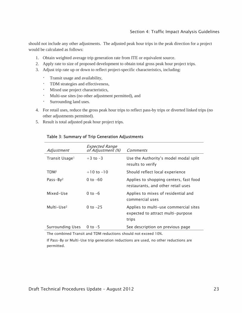
should not include any other adjustments. The adjusted peak hour trips in the peak direction for a project would be calculated as follows:
1. Obtain weighted average trip generation rate from ITE or equivalent source. 2. Apply rate to size of proposed development to obtain total gross peak hour project trips. 3. Adjust trip rate up or down to reflect project-specific characteristics, including:
· Transit usage and availability, · TDM strategies and effectiveness, · Mixed use project characteristics, · Multi-use sites (no other adjustment permitted), and · Surrounding land uses.
4. For retail uses, reduce the gross peak hour trips to reflect pass-by trips or diverted linked trips (no other adjustments permitted).
5. Result is total adjusted peak hour project trips.
TTable 33: Summary of Trip Generation Adjustments
Adjustment Expected Range of Adjustment (%) Comments
Transit Usage1 +3 to –3 Use the Authority’s model modal split results to verify
TDM1 +10 to –10 Should reflect local experience
Pass-By2 0 to –60 Applies to shopping centers, fast food restaurants, and other retail uses
Mixed-Use 0 to –6 Applies to mixes of residential and commercial uses
Multi-Use2 0 to –25 Applies to multi-use commercial sites expected to attract multi-purpose trips
Surrounding Uses 0 to –5 See description on previous page The combined Transit and TDM reductions should not exceed 10%.
If Pass-By or Multi-Use trip generation reductions are used, no other reductions are permitted.

Technical Procedures Update
24 Draft Technical Procedures Update – August 2012
44.4 Trip Distribution and Assignment Few development projects will be large enough to justify a special run of the Countywide Model to distribute and assign project trips. Instead, project generated trips can be distributed and assigned manually using the model to predict background traffic. Existing directional split information, turning movement counts and local knowledge may all contribute to predicting the distribution of project trips.
For most projects, manual assignment techniques can adequately assess intersection impacts. Manual as-signment requires the engineer or planner to estimate the likely routes that traffic generated by the project would use. Computer programs have been developed to assist in the manual assignment process by doing the mathematical bookkeeping for the engineer or planner. They are generally available to local jurisdictions at a reasonable cost. Manual assignment programs may be developed using any spreadsheet program such as Excel or a software package such as TRAFFIX.
The local jurisdiction should also attempt to maintain an inventory of “approved trips”. This inventory can be maintained on any of the above programs or a separate database. This database would include existing traffic counts plus the anticipated turning movement volumes from approved projects. This information is extremely useful in obtaining consistency among traffic impact studies and provides the basis for analyzing cumulative traffic impacts.
4.5 Selection of Study Intersections Study intersections will be selected after local staff have completed and approved the trip generation, distri-bution and assignment. As a rule, the analysis should include any signalized intersection to which at least 50 net new peak hour vehicle trips would be added by the project. This level of impact will normally reflect a one to three percent increase in critical volumes. Projects just meeting the threshold for traffic impact analy-sis will normally require analysis of only the intersection(s) adjacent to the site. Larger developments will require the analysis of a larger number of intersections. Engineering judgment may be used to eliminate in-tersections from the analysis that are not controlling intersections or where critical movements are not affect-ed as the project only adds through movements. The elimination of study intersections where 50 or more trips are projected to be added by the project should be done in consultation with the city engineer or trans-portation engineer for the local jurisdiction in which the affected intersection is located. The traffic study should also fully document the rationale for eliminating intersections from the analysis.
Evaluation of unsignalized intersections may also be considered for analysis. Traffic counts at study inter-sections should be conducted in accordance with the Traffic Counting Protocol shown in Appendix B.
Study intersections should be selected without consideration for jurisdictional boundaries. Study intersec-tions should also include arterial and ramp intersections defined as Routes of Regional Significance, as ap-propriate. When the proposed project adds more than 50 net new peak hour vehicle trips to a freeway ramp, then the impact of the project on freeway MTSOs should be evaluated. Project-specific impacts should be mitigated at these locations consistent with the Action Plans adopted by the RTPCs.

Section 4: Traffic Impact Analysis Guidelines
Draft Technical Procedures Update – August 2012 25
44.6 Analysis A Traffic Impact Analysis is to consider the potential impact of a project on transportation conditions using performance measures and standards contained in the local General Plan, the MTSOs from the Action Plan for Routes of Regional Significance, and the standards for the CMP network. The results of the analysis should be compared with standards set forward in these documents. Other measures of performance or im-pact may also be included to provide a more comprehensive multi-modal assessment of the projects potential effects including quality and safety of service. . The traffic impact analysis should include, as a minimum, consideration of the following scenarios:
Existing conditions at or near the time of analysis (Existing Conditions); Existing conditions plus the project (Existing Plus Project Conditions); Future-year baseline conditions for a forecast year at some time after the year the project being ana-
lyzed is to be implemented. The conditions will include all approved land use changes and any de-velopment that is consistent with the General Plan and expected to occur within the time frame of the project. It will also include transportation projects programmed for implementation prior to the fore-cast year and any approved mitigation measures required for approved or planned projects. This scenario will be used with the next to identify the incremental cumulative impact of the project. (Fu-ture Year No Project Conditions); and
Future-year baseline conditions plus the project that is being analyzed. This condition should in-clude all mitigations proposed for the project to meet applicable standards (Future Year with Pro-ject Conditions).
For projects expected to be phased over several years, the analysis horizon should extend beyond completion of the final phase, but separate traffic analysis may be required for each phase depending on the size of each phase and the time between phases. All capital improvements in the Capital Improvement Program that will affect traffic capacity at the study intersections should be considered in the cumulative traffic impact analy-sis.
Analysis of levels of service (LOS) is required when the threshold of significance in the CEQA document includes LOS standards. LOS should be calculated for each study intersection for the weekday morning (AM) and weekday evening (PM) peak hours as appropriate. For certain types of development, including some retail or recreational uses, midday or weekend day LOS calculations may be appropriate. Selection of additional peak periods for study will be at local discretion.
Roadway LOS at signalized intersections should be calculated using the 2010 Highway Capacity Manual operational method unless the calculation is being compared to an MTSO or other standard that was estab-lished using the methodology previously adopted by the Authority (CCTALOS), in which case the CCTALOS method may be used. To ensure consistent application of procedures for analyzing LOS at sig-nalized intersections in Contra Costa, guidelines have been developed for how each procedure should be ap-plied and the parameter or default values should be used. Guidelines for the use of the 2010 Highway Ca-pacity Manual operational method in Contra Costa are provided in Appendix C and guidelines for the use of the CCTALOS methodology in Contra Costa are provided in Appendix D. Potential impacts from vehicle

Technical Procedures Update
26 Draft Technical Procedures Update – August 2012
queuing may be estimated using analysis programs, such as Synchro II or HCS-Signal, that apply queuing analysis procedures of the 2010 Highway Capacity Manual. Guidelines for the estimation of other MTSOs besides intersection LOS are contained in Appendix A.
Although not required specifically by Measure J, CEQA requires an analysis of air quality impacts if a pro-ject exceeds specific thresholds. These thresholds vary according to the criteria pollutant. Thresholds have been established for Reactive Organic Gases (ROG), Oxides of Nitrogen (NOx), Carbon Monoxide (CO), Particulate Matter (PM10 and PM2.5), and Greenhouse Gases (GHG). Measures must be identified and evaluated that will mitigate the negative air quality impacts of the projects if the threshold level is exceed-ed.11. The GHG analysis is not required and the threshold values do not apply if it can be demonstrated that the project is in compliance with a “Qualified GHG Reduction Strategy.” Projects classified as “Transit Pri-ority” are also exempt from the GHG analysis requirement if certain conditions are met including but not limited to the following12:
The project includes affordable housing or includes payment of an in lieu fee for affordable housing or provides public open space equal to or greater than five acres per 1000 new residents.
The project does not exceed eight acres or 200 residential units.
44.7 Multi-Modal Level of Service In Contra Costa as in many other parts of the country, there has been growing interest in level of service for modes other than automobile. Procedures for qualifying level of service for pedestrians, bicyclists and transit users have been developed and used by many local regional and state agencies over the years, but a standard-ized methodology has been developed by a national committee and documented in the 2010 Highway Capac-ity Manual. The 2010 Highway Capacity Manual provides a quantitative methodology for defining level of service by roadway segment separately for pedestrians, bicyclists and transit. Methods are also provided for pedestrian and bicycle level of service at intersections. While there has not yet been adequate use of these methods in Contra Costa to warrant specifying their use in fulfillment of the Measure J Growth Management requirements, they should be considered whenever multimodal analyses of impacts of development or bene-fits from transportation improvements are considered. They also offer additional options for the MTSOs as the Action Plans are updated.
4.8 Mitigation Measures Projects included in the Capital Improvement Program that may affect traffic impact study intersections should be analyzed in the Future Year Baseline Conditions and the Future Year Baseline Plus Project Condi-tions scenarios. This program could include a local traffic mitigation fee or a requirement that each devel-
11 Bay Area Air Quality Management District, California Environmental Quality Act: Air Quality Guidelines, Updated May 2011, page 2-1.
12 Institute for Local Government, Evaluating Greenhouse Gas Emissions as Part of California’s Environmental Review Process: A Local Official’s Guide, Sacramento, CA, September 2011.

Section 4: Traffic Impact Analysis Guidelines
Draft Technical Procedures Update – August 2012 27
opment provide funding for its share of cumulative impacts. Measure J also requires each local jurisdiction to participate through the appropriate RTPC in a regional transportation mitigation program.
Three options exist under CEQA when the traffic impact analysis identifies significant impacts even after mitigation through the 5-year Capital Improvement Program or conditions on the project:
Modify the project so that all study intersections meet adopted standards or objectives; As part of the CEQA process, adopt a Findings of Overriding Considerations indicating that consid-
erations other than traffic justify the proposed projects; or Deny the project.
Approval of the project without following these procedures may result in noncompliance with the Authori-ty’s Growth Management Program, and subsequent withholding of Local Street Maintenance and Improve-ment funds.
44.9 Traffic Impact Report The required traffic impact report must fully document the approach, methodology, and assumptions of the traffic analysis. It should clearly explain the reasons for any adjustments to the weighted average trip gen-eration rates and assumptions used for trip distribution and assignment. Figures should be used to help illus-trate those assumptions. The report should summarize the results of any calculations in table form or in a figure and include the traffic volumes and calculation sheets as an appendix to the report. Recommended mitigation measures should be clearly stated and should indicate the relative share of the mitigation costs assigned to the project. Results for the study intersections should be calculated with and without the pro-posed mitigation measures. A typical traffic impact report is outlined in Appendix E.

Technical Procedures Update
28 Draft Technical Procedures Update – August 2012
This page left blank intentionally

Draft Technical Procedures Update – August 2012 29
55 TRAVEL DEMAND FORECASTING
5.1 Overview of the Countywide Model The analysis of the transportation system as a whole and of its components, as well as its relationship to land use decisions, requires an understanding of potential future travel patterns. Computerized travel demand forecasting models originally developed by transportation researchers in the 1960’s are now broadly accepted and widely applied throughout the international transportation engineering community. Typically, these models use land use, transportation-supply, and demographic information to predict future travel demand and mode of travel, and are considered by industry professionals to be the best tool available for evaluating the impacts of significant changes in land use policies or major improvements to the transportation system. This section of the Technical Procedures provides an overview of the Authority’s computerized travel demand forecasting model (the Countywide Model) and summarizes the specifications, policies and procedures. Model users are encouraged to obtain from the Authority the detailed CCTA Model User’s Guide
13 for oper-
ating the model.
The purposes of the Authority’s travel model are:
For use in developing Action Plans required as part of the adopted Growth Management Plan As a consistent technical tool for use by local jurisdictions in the analysis and updating of local Gen-
eral Plans as may be necessary to incorporate the Growth Management Element To assess the traffic impacts of Specific Plans, General Plan Amendments, and projects that generate
more than 100 net new peak hour vehicle trips To fulfill the requirements of the Congestion Management Program (CMP) function, such as identi-
fying trips that can be discounted in an Exclusions Study To assess project impacts for Strategic Plan Project Delivery (Measure J), Corridor Studies , design
studies, and EIR/EIS studies For the analysis of CMP deficiency plans Development of regional mitigation and fee programs CEQA-related analysis of the above-listed uses
The usefulness of the model in analyzing major amendments to a General Plan or in studying major transpor-tation corridors is well documented. The travel demand forecasting model is less useful in the analysis of
13 Cambridge Systematics with Dowling Associates and Caliper Corporation, Decennial Model Update – CCTA Model User’s Guide, prepared for the Contra Costa Transportation Authority, Pleasant Hill, CA, June 2003.

Technical Procedures Update
30 Draft Technical Procedures Update – August 2012
minor changes in the street network or in demand management programs. Table 4 provides examples of both appropriate and inappropriate uses of the models.
TTable 44:: Examples of Appropriate and Inappropriate Model Appplications
Appropriate Applications Inappropriate Applications
Assessing traffic impacts of a de-velopment project or a major change in General Plan Land Uses
Quantifying shifts in congestion within a longer peak period
Assessing traffic impacts of a new major roadway
Evaluating impacts of a new right turn lane at an intersection
Estimating through traffic in a cor-ridor
Evaluating through traffic at an inter-section
Estimating regional changes in transit ridership
Estimating the potential for casual car-pooling at an existing transit station
Estimating changes in travel pat-terns over time
Measure J required that the Authority develop and maintain a travel demand forecasting model that would support multi-jurisdictional participation in the Growth Management Program. The Congestion Management Program (CMP) further requires that the Authority, as the Congestion Management Agency (CMA) for Con-tra Costa, maintain a land use database and travel forecasting model that is consistent with the region’s data-base and model. The CMA is also responsible for specifying which components of the model to apply for various types of analysis.
The Authority’s Countywide Model was adapted from the model maintained by the Metropolitan Transporta-tion Commission (MTC), and focuses on Contra Costa and the Alameda County portions of the Tri-Valley, including Dublin, Livermore, and Pleasanton. The Countywide Model is available for use by public agencies and private consultants throughout Contra Costa. It comprises the uniform transportation analysis tool that ensures consistency among traffic projections, even when they are prepared by different and sometimes competing entities.
The RTPCs should use the Countywide Model to undertake Action Plan updates, and local jurisdictions should use the model for General Plan updates, traffic impact studies, and related growth and congestion management efforts. Furthermore, the Authority will use the Countywide Model to evaluate MTSOs on the regional system, and future congestion on the CMP network. Various agencies, including the Authority, Cal-trans, and local jurisdictions, are also encouraged to use the Countywide Model for corridor studies, envi-ronmental review, and project-related planning and design.
MTC has recently developed an activity-based model for the Bay Area (Travel Model One) that will ulti-mately replace the current trip-based model (BAYCAST-90). Both MTC’s BAYCAST-90 model and the

Section 5: Travel Demand Forecasting Models
Draft Technical Procedures Update – August 2012 31
CCTA model are trip-based models in which person trips are treated independently in the model. There is no explicit recognition of trip chaining or of household planning of daily trips by household members. An ac-tivity-based model is a disaggregate model of household trip making that can account for the linking of mul-tiple household trips into tours, as opposed to the trip-based model that is an aggregate model of zone-to-zone travel that analyzes trips independently and without providing any connection between them.
As the CMA for Contra Costa, the Authority is required to maintain and update a travel demand forecasting model consistent with MTC’s model and the Association of Bay Area Governments (ABAG) projections database. At present, MTC allows CMAs to demonstrate consistency with either the trip-based BAYCAST-90 model or the new activity-base Travel Model One. In 2010 the California Transportation commission adopted guidelines that suggested that only the largest Metropolitan Planning Organizations in the state should undertake the development of activity–based models because of the additional complexity of model development and the additional data requirements of the model.
14 The guidelines suggested that smaller or-
ganization retain a trip-based modeling structure. Consistent with this guidance, the Authority has chosen to retain a trip-based structure.
The Authority’s Countywide Model is calibrated to 2000 traffic counts and also makes use of 2010 count data, which, due to the “Great Recession” was generally found to be lower than the 2000 counts, and was therefore used for sensitivity testing rather than full calibration. The land use database generally reflects the most recent set of land use projections from ABAG. Internal model components match those of the MTC model.
In addition to the MTC capabilities, the Countywide Model includes the following key features:
Dynamic Scenario Creation: The new model structure allows for the easy creation of any sce-nario between the base year (2000) and the “out year” or future time horizon. The land use forecasts for any study year will be directly available along with the respective network and transit improve-ments for that year.
Improved Database for Traffic Counts: A comprehensive user-friendly database for traffic counts was populated to facilitate use of available count data. The database format is linked to a set of geographic plots that illustrate the traffic volume information in a user-friendly map format.
Greenhouse Gas (GhG) Estimator: A process to estimate the greenhouse gas emissions from transportation is included in the updated model.
The Countywide Model runs on the TransCAD® software platform. The software incorporates traffic as-signment algorithms that can rapidly and accurately compute traffic flows and estimate mode choice. The GIS enhancements and native support for many different database types makes the model more user-friendly.
Within Contra Costa, the Technical Modeling Working Group (TMWG) has helped to guide the Authority’s model development process. The TMWG serves as a subcommittee to the Authority’s Technical Coordinat-
14 California Transportation Commission, 2010 California Regional Transportation Plan Guidelines, Sacramento, CA, April 12,
2010.

Technical Procedures Update
32 Draft Technical Procedures Update – August 2012
ing Committee (TCC). The TCC initially created the TMWG specifically to address issues of model care, “feeding”, and application through the congestion and growth management program. In 1998, the TCC as-signed the TMWG the responsibility to oversee and guide technical aspects of the decennial model update. As issues arise, the TMWG reports its recommendations to TCC for consideration and adoption. The TMWG oversees the modeling specifications, policies, and procedures set forth in this section and antici-pates reviewing and updating them periodically.
55.2 Countywide Model Input Requirements The Countywide Model incorporates MTC’s BAYCAST-90 five-step forecasting process (auto ownership, trip generation, trip distribution, mode split and assignment) to predict travel patterns. The Countywide Model includes data from local jurisdictions within Contra Costa and the Tri-Valley and is consistent with data developed by ABAG. As a result, the travel forecasts reflect the cumulative effect of predicted changes in land use and planned roadway improvements within the framework of MTC’s Regional Transportation Plan for the Bay Area.
The traffic analysis zones (TAZs) in the Countywide Model began with MTC’s 1,099-zone model for the Bay Area that existed at the time the Countywide Model was first developed. Then, approximately 1,700 TAZs were added in the Contra Costa/Tri-Valley Study Area. The current model consists of 3,120 TAZs, of which 1,495 are located within Contra Costa.
Land use and demographic data are required for each TAZ. The demographic data provides the basis for estimating trip generation. Both the demographic and transportation network data are used in predicting trip distribution patterns and mode of travel. The model land use and demographic inputs for traffic zones within Contra Costa consist of the following ten variables:
Number of Households Household Population Employed Residents Household Income (expressed in 2000 dollars)15 Retail Employment Service Employment Other Employment Total Acres within the Zone High School Enrollment College Enrollment
The land use data for the model is updated every two to four years through the allocation of ABAG’s new Projections series data. The Authority’s Land Use Information System (LUIS) provides land use data sets that correspond with the following levels:
15 Household income feeds into MTC’s auto ownership model and is later considered in trip distribution and mode split.

Section 5: Travel Demand Forecasting Models
Draft Technical Procedures Update – August 2012 33
. Development that existed and was occupied in the base year. The current model is set up to run for years 2000, 2010, and ten-year increments thereafter, through 2040. In addition, through interpolation, the model is capable of running any intervening year (such as 2017).
. Development that received approval from a city or the County but was either not constructed or not occupied in the base year but corresponds with a 5 to 10-year outlook.
. Development projects considered likely to be completed within the next 20 years but that have not yet to complete the approval process.
. Development potential remaining in each traffic zone after completion of all approved and proposed projects based on General Plan designations and probable market forces in a 25 to 30 year time frame or beyond.
The first LUIS database was issued by the Authority in 1992, and reflected consistency with ABAG’s Pro-jections ‘90 forecasts. The LUIS has been updated numerous times since then using the most recent ABAG projects. Further updates will continue as necessary to maintain consistency with the regional model.
The LUIS is public record and is available to local jurisdictions, other public agencies, and interested mem-bers of the public and private sector. These data are useful for a variety of planning applications beyond transportation, including energy and water resource assessment.
For areas outside of Contra Costa and the Tri-Valley, the TAZ structure is equivalent to MTC’s zone system. Data for these zones are taken directly from MTC’s model.
The highway and transit networks for the Countywide Model are based on the existing and planned transpor-tation system, including freeways, arterials, major collectors, and selected minor collectors and include virtu-ally all signalized intersections in the study area. The transit network is based on MTC’s transit networks with refinements based upon local review by the transit operators. For both highway and transit networks, detailed networks within Contra Costa have been combined with MTC networks outside the county.
The Countywide Model uses the auto ownership, trip generation, trip distribution and mode choice modules within MTC’s BAYCAST-90 model.
55.3 Output Options The Authority’s Countywide Model can generate highway and transit outputs for the AM and PM peak hour, AM and PM peak period (four hours), and daily traffic volumes. Output from the model can be provided in the form of data listings and/or computer plots. Examples of model output include link volumes, intersection turn movements, volume-to-capacity (v/c) ratios, vehicle miles traveled (VMT), vehicle hours traveled (VHT), and vehicle hours of delay. The model provides sufficient detail to permit travel demand forecasts down to the level of minor collector roadways. However, it does not include residential streets.
5.4 Link-Level Output Adjustments Ideally, the Authority’s models should be well validated on all links. Other factors, such as variations in traf-fic count data and budget limitations, however, make it unfeasible to continue the validation adjustment pro-

Technical Procedures Update
34 Draft Technical Procedures Update – August 2012
cedures indefinitely. At some point, the model validation effort must reach closure. The point of closure occurs when the links in the model have been validated to the extent necessary to meet the validation targets established in this document. To account for any remaining differences between base-year model output and actual counts, a link volume adjustment process has been established.
As illustrated in Figure 4, the process involves assessing the difference between actual counts and base-year model outputs. The “Model Correction Volume”, which is the difference between existing counts and the base-year validation model run, is applied to the base year and projections.
When developing intersection turning movement forecasts, the adjustment process should be applied to inter-section approach and departure volumes, as described in the next subsection. Alternatively, link-level ad-justments can be made within the forecasting model through the implementation of the Origin-Destination Matrix Estimation (ODME) process, as described in Appendix F.
55.5 Intersection Turning Movements and Level-of-Service Options While the Countywide Model will store intersection turning movements, separate software is needed to cal-culate levels of service at signalized intersections. To obtain reasonable intersection turning movements from the model, adjustment of the raw model output is required using a technique known as the Furness method. This adjustment technique has been automated and is summarized below and in Figures 4 and 5.
Step 1 Calculate the Model Correction Volume—that is the difference between the projected peak hour vol-ume for the validation run and actual peak hour traffic volumes—for each network link.
Step 2 Determine the forecast peak hour approach and departure volumes for each signalized intersection to be studied by adding the Model Correction Volume to the model output.
Step 3 Develop turning movement volumes that are consistent with the approach and departure volumes by balancing projected turning movements with actual turning movement volumes using an iterative process. This balancing process is summarized in Figure 5.
Step 4 Check reasonableness by comparing adjusted turning movement volumes with both the existing count data and the raw model output.
Step 5 Review volume adjustments that do not appear reasonable and, if appropriate, revise adjustments.
This methodology works well except when:
The model network places a centroid connector at an intersection. The future forecast adds a new leg to an intersection. A major new roadway is located near an intersection.
In the first case, the network coding should be carefully checked in the study area, and zone centroid con-nectors should be moved to a new location that is adequately removed from adjacent intersections.

Figure 4
Link Adjustment Process
Validation Year Existing Traffi c Counts
2010, 2020, 2030, 2040...
Alternative Runs
Trip Tables Build Networks
Validation Model
Run
Validation Year Trip TableExisting Network
Validation Model Run— Existing Counts
= Model Correction Volume
Model Validation
Future Model Output+ Model Correction Value= Adjusted Model Output
Go to Figure 5

Figure 5
Intersection Turning Movement Adjustment Process
(The “Furness” Method)
Sa
Sd
Nd
Na
E dW
aWd
Ea
EAST
NORTH
SOUTH
WES
Tl t r
lt
r
lt
r
r t l
Traffi c counts provide data on observed turn-ing movements — left (l), right (r) and through (t) — at intersections
The travel demand model provides estimated ap-proach (a) and departure (d) volumes for intersec-tions. These volumes are adjusted using the link ad-justment process shown in Figure 4
— Nt Wr El = Nd
Ratio
of o
bser
ved
turn
ing
mov
emen
ts
to fo
reca
st v
olum
es Nd
St — Wl Er = Sd Sd
Sl Nr — Et = Ed Ed
Sr Nl Wt — = Wd Wd
= = = =
Sa Na Wa Ea
Ratio of observed turning movements to forecast volumes
Sa Na Wa Ea
“Furnessed” (i.e., Adjusted) Peak-Hour Intersection Turning Volume Projections
Step One:“Seed” the Initial MatrixObserved traffi c counts are used to create the initial matrix of turning movements and approach and departure volumes
Step Two:Balance Observed and Forecast Volumes The ratio of observed turning movements to forecast approach and departure volumes is used to adjust the turning movement matrix. The forecast approach volumes (columns) and the forecast departure volumes (rows) are adjusted iteratively until the matrix “closes”.
Step Three:Check Reasonableness of ResultsAn intersection-by-intersection compari-son of the adjusted volumes to both ob-served and forecast volumes is necessary to check for potential anomalies.

Section 5: Travel Demand Forecasting Models
Draft Technical Procedures Update – August 2012 37
The second exception introduces a more difficult challenge because there is no existing data that can be used to validate the approach volume for a new leg to an intersection. The Furness process in this case may be bypassed, and the analyst may elect to use the raw model output data if it appears reasonable or they may elect to perform manual adjustments as appropriate. If the Furness method is used, approach and departure volumes from the model output should be carefully checked and, if necessary, adjusted. The Furness matrix may be “seeded” with the raw turning volumes from the forecast model output.
16 The traffic analyst also has
the option of inputting hand-calculated approach volumes based upon Institute of Transportation Engineers (ITE) vehicle trip generation calculations for the land uses on the road leg being added to the intersection.
The final exception could occur when the model includes a major new roadway near the intersection. In this case, manual adjustments may be needed where the distribution of forecast approach and departure volumes change significantly.
55.6 Select Link Analysis The Countywide Model is capable of performing select link analysis that can identify the origin and destina-tion zones for traffic on a specific network link. Select link analysis may be used for defining benefit dis-tricts for fee programs, assessing percentages of through traffic for Routes of Regional Significance, and evaluating traffic exclusions for CMP LOS monitoring. The origin-destination information is generated by the trip assignment module of the TransCAD model and the analysis is referred to as Critical Link Analysis. Where feasible, the results of select link analysis should be compared with observed origin-destination sur-veys to determine the level of validation for the specific link that is being analyzed.
5.7 Gateway Constraints As outlined in Appendix F, the Countywide Model can be used directly to adjust peak hour volumes on ma-jor routes. This type of adjustment, called Gateway Constraints, may be necessary under two scenarios: 1) When further adjustments to the model are required to meet the observed model validation targets, or 2) When future traffic volumes generated by the model are excessively high and need to be adjusted to account for known capacity constraints or bottlenecks at a specified location.
5.8 Model Specifications The Countywide Model is fully consistent with MTC’s model. Any revisions undertaken to the Authority's models must therefore conform to the specifications set forth below and be consistent with MTC’s model. As MTC’s model continues to evolve, the Authority may periodically update the Countywide Model to re-flect MTC’s model, provided those updates are feasible, practical, and cost effective.
16 Note: “Seeding” the Furness matrix with zeros will result in a turning movement output of zero. To obtain reasonable output for
the new approach leg, the matrix must be seeded with non-zero, positive integers. The raw model output turning volumes should suffice for this purpose.

Technical Procedures Update
38 Draft Technical Procedures Update – August 2012
TTRIP GENERATION
Trip production and attraction models are based on household survey data from the most recent trip-based MTC BAYCAST-90 model, which is based on the MTC Travel Surveys used to develop the Regional Transportation Plan. This approach results in models that reflect unique Contra Costa travel behavior char-acteristics. The models produce estimates of average daily (weekday) person trips by individual trip purpose using cross-classification at the production end and linear regression at the attraction end.
The basic regional trip purposes—Home-Based Work, Home-Based Shopping/Other, Home-Based So-cial/Recreational, Home-Based School and Non-Home-Based—are drawn from the MTC model,
17 which was
calibrated to the observed data. Home-Based School trips are further separated into grade school, high school and college. Specific production and attraction models are estimated and validated for each indicated trip purpose.
As specified in the model documentation, special generators were developed for regional parks, regional shopping centers, unique industrial areas and large concentrations of senior housing (in excess of 4,000 units) that have unique trip generation characteristics. Schools will not need to be identified as special generators since these are specifically identified as separate trip purposes.
The trip generation equations used in the Authority’s models will permit consideration of transportation de-mand management (TDM) strategies. The equations, however, are used consistently for all TAZs. Assign-ing different trip generation rates for individual TAZs to reflect differing levels of TDM is possible but not recommended. Alternatively, analysis of the potential impacts of TDM can be incorporated into the traffic impact analysis conducted as part of development review.
TRIP DISTRIBUTION
Trip distribution is done using a standard gravity model approach with a large number of iterations to ensure better closure to the target trips and productions. The Countywide Model is capable of incorporating the three dimensional matrix balancing within TransCAD to implement the trip distribution. This technique can be applied to ensure that the county-to-county trip movements match MTC county-to-county trips (this is the third dimension of the balancing process). The Countywide Model accomplishes consistency with MTC’s county-to-county trip tables by virtue of the model’s strict adherence to the MTC model structure and algo-rithms as they exist for the RTP. As MTC’s model continues to evolve, diversion from the county-to-county trip tables may require application of the “third” matrix balancing dimension. Should MTC migrate to a tour-based model, then three-dimensional balancing will become mandatory. The model should be iterated until closure is reached. Because gravity models are highly sensitive to zone size, the MTC F-Factor values have been re-calibrated for use in Contra Costa. Any factors used in the validation must be held constant for the forecast horizon years.
17 Travel Demand Models for the San Francisco Bay Area (BAYCAST-90) Technical Summary, Metropolitan Transportation
Commission, Planning Section, June, 1997.

Section 5: Travel Demand Forecasting Models
Draft Technical Procedures Update – August 2012 39
The TransCAD software performs matrix balancing for attractions and productions, rather than the tradition-al normalization to attractions only. The model explicitly represents in-commuting workers from outside the nine-county Bay Area. External trip matrices were developed from MTC external trip tables and updated with origin-destination surveys that were available in the vicinity of these externals at the time of the decen-nial model update. As new information becomes available from MTC, adjoining counties, and other MPOs, the external trip matrices may be updated.
The TransCAD setting for trip distribution matrix balancing should be set at a minimum of 100 iterations to ensure closure of the matrix balancing process.
The MTC consistency requirements state that county-to-county home-based work and total person trips should match MTC trip tables within one percent or 10,000 trips, whichever is higher. The three-dimensional balancing approach should ensure that this consistency requirement is met.
MMODE CHOICE
Each of MTC's regionally estimated mode choice models is implemented directly as part of the Countywide Model update. The 2,700 zone system has a fully functional mode choice estimation model for all zones. Adjustments may be made to each model’s bias constants to reflect (1) the change in zone system size and definition, and (2) the differences in transit path building when using TransCAD instead of MTC’s CUBE multi-path-building algorithms.
For Home-Based Work trips, total person trips are split into walk, bike, transit-walk access, transit-drive ac-cess, drive-alone auto, 2-person auto, and 3+ person auto using a multi-modal logic model. The Authority’s Countywide Model estimates 2 person and 3+ person HOVs for Home-Based Work, Home-Based Shop/Other and Home-Based Social-Recreational trips, and provides for their separate assignments on the highway network. The mode choice models are applied for all inter-and intra-county trips, rather than in previous models where the inter-county mode shares were derived directly from the MTC trip tables. This will require that, for mode choice and assignment purposes, both the transit networks developed for the full nine-county area and the highway networks must be retained for all modeling applications.
AUTO OWNERSHIP AND OTHER MODE SPLIT MODEL INPUT ASSUMPTIONS
To maintain consistency with MTC’s model, estimates of model input assumptions for the base and future year mode split—such as auto ownership levels, income, auto operating costs, tolls, fares, and parking costs—are obtained directly from the latest approved and published MTC regional model forecasts for the RTP. Use of these estimates provides the ability to reflect the dynamic influence of changing auto ownership patterns on mode choice without relying upon less sophisticated and more aggregate cross-classification or regression estimates. The Authority implements these types of updates to the model as part of the periodic model update process.

Technical Procedures Update
40 Draft Technical Procedures Update – August 2012
TTRAFFIC ASSIGNMENT
Vehicle trip tables are created directly from the mode choice model output for three individual time periods: AM peak period (6 to 10 AM), PM peak period (3 to 7 PM), and the off-peak period (all remaining hours). Traffic volumes resulting from the peak period assignments are further processed to produce AM peak hour and PM peak hour volumes. Vehicle occupancies used to calculate vehicle trips by purpose are based upon MTC’s occupancies. The conversion of daily vehicle trips to each individual time period was based initially upon the MTC Travel Survey diurnal distribution factors provided by MTC. The conversion can be modified subsequently based upon comparisons of actual and estimated traffic volumes by link. These factors may be modified only where a systematic pattern exists (for example, peak spreading evident on the Bay Bridge) or where an obvious variation from the time period of analysis exists (for example, the attraction of trip ends in the AM peak hour for major regional shopping centers occurs near the end of the AM peak period, and spills over into the off-peak).
Vehicle trip assignments are made for each time period using the stochastic user equilibrium assignment al-gorithm available within TransCAD software. Following these assignments, a daily traffic volume is calcu-lated by summing the volumes from the three time periods. Output transit trips are created for the same three time periods and assigned to the transit networks.
Park-and-ride vehicle trips to BART stations are included in the highway assignment. Transit park-and-ride trips are initially estimated during the transit path-building step, representing one leg of a transit trip where park-and-ride trips go from a TAZ to a nearby BART station. A matrix of park-and-ride vehicle trips is cre-ated and added to the AM peak hour vehicle trip matrix for assignment. For the PM peak hour, the matrix is transposed and then added to the trip table for assignment.
INTER-COUNTY TRIPS
Inter-county trips are defined as those trips that have one or both endpoints outside of Contra Costa but still within the nine-county MTC region.
18 The Countywide Model treats inter-county trips the same as intra-
county trips.
Inter-county trips are estimated using the same models as the internal trips for Contra Costa. This approach is possible because the 2,700-zone Countywide Model contains the full level of detail for MTC zones so that the models can be applied easily to any geographic study area.
REGIONAL EXTERNAL TRIPS
Regional external trips are defined as those trips with one endpoint outside of the MTC nine-county Bay Ar-ea. External through trips and transit trips are considered negligible.
18 Internal zones for the Decennial Model are defined as any of the detailed zones within the previous four subarea models. For
the Tri-Valley model, this included the Tri-Valley portion of Alameda County.

Section 5: Travel Demand Forecasting Models
Draft Technical Procedures Update – August 2012 41
The Countywide Model addresses trips that enter and leave the MTC region on State Route 4, I-580 and State Route 17, specifically. This was implemented by including production and attraction estimates by pur-pose for these highways at the point where they enter the MTC region. These estimates of external trips are added to the external trip tables developed by MTC for all other regional external stations. Transit trips com-ing in from external stations are added to the transit trip tables where appropriate. The ACE train, for exam-ple, constitutes an external transit link. External trip tables are added to the internal trip tables prior to the application of peaking factors so that they are included in all time period trip tables. External trip tables can be developed either as vehicle trips (for auto assignments) directly or as person trips (for transit assignments) based on the origin of the data used to estimate these tables.
The Countywide Model could conceivably be expanded to include San Joaquin County as a part of the TAZ structure rather than as an external. In Santa Clara County, the VTA has taken steps to add some outlying counties. In Solano County, the CMA uses a combined MTC/SACOG model. Until MTC decides to expand its model, the external counties in its model will continue to be treated using a trip-table technique to esti-mate in-and-out commuting for the Bay Area. Should the Authority choose to explore the addition of TAZs outside of the Bay Area, either in the context of the Countywide Model, or for a specific corridor study, the expanded model would be developed in consultation between the Authority and MTC.
TTHE LAND USE INFORMATION SYSTEM (LUIS) DATABASE
The Authority maintains a detailed LUIS as part of its modeling effort. As shown in Figure 6, the Authori-ty’s LUIS is based upon the initial inputs received from ABAG at the census tract level and provided to the CMAs. Over the years, MTC has expanded its TAZ structure representing the Bay Region from 1,099, to 1,452, and then to 1,792 zones. MTC’s model includes approximately 150 TAZs in the Contra Costa study area. Within the Authority’s model study area, a 10-fold more fine-grained TAZ system is applied to the Countywide Model. For the remaining Bay Area, however, the TAZ structure of the Countywide Model re-flects the 1454 TAZ level, though it could be expanded in the future. Further disaggregation within the mod-el study area is performed through an allocations model that assigns households and jobs to the Countywide Model TAZ system based upon available land use information, aerial photography, and local input. The LUIS is comprised of approximately 1,700 zones.
Full documentation of the LUIS approach, methodology, and results are available in separate reports. Future travel demand forecasts are generally prepared for the near-term (5 to 10 year), the mid-term (15 to 20 year) and the long-range (25 to 30 year) time horizons. The land use changes for each of these planning pe-riods was estimated based on the remaining development potential (vacant capacity) in each zone, given General Plan zoning and likely market forces. Citywide and census tract forecasts are controlled to ABAG forecast totals. The land use data results are then reviewed by the local jurisdictions to ensure consistency with local General Plans.
Subsequent updates to the land use database will continue to be made by disaggregating ABAG’s latest Pro-jections series data by census tract, in accordance with the latest available information for vacant capacity and based upon the zonal allocations.

Concord
WalnutCreek
PleasantHill
Alamo
1770 1772
1778
17791782
1783 17871792
1800
1803
1804
1807
1821
1826
182718381842 1851
185218611862
1865 1867
1875
1884
1886
1887
1888
1898 1901
19091913
1922
ABAG releases Projections 2XXX,forecasts at county and city levelfor the entire Bay Area.
ABAG publishes Projections2XXX, forecasts at census tractlevel for the entire Bay Area.
MTC allocates ABAG census tractlevel forecasts to MTC’s RegionalModel TAZs for the entire Bay Area.
CCTA allocates MTC TAZ-levelforecasts to Countywide ModelTAZs within Contra Costa Countyand Tri-valley.
Local jurisdictions review TAZ-level data for Contra Costa Countyand Tri-valley.
CCTA approves land useallocations for Contra CostaCounty and Tri-valley.
Figure 6LUIS Methodology
Draft Technical Procedures Update – August 2012 43
Complete documentation of the LUIS methodology, approach, and results is available from the Authority upon request. The LUIS uses Microsoft Access® software.
BBASE AND SUBAREA NETWORKS
The highway and transit networks for the Countywide Model were initially developed by combining the four subarea model networks and updating the attributes to represent a calibration year. These networks were then combined with the MTC validation networks and adjusted for any differences that may have occurred between the calibration years of the models. The capacity, speed, frequency, dwell time, walk access, auto access, and transfer network coding conventions used in the Countywide Model were reviewed and updated. These updated conventions have been maintained when new transit and highway network details were added.
External highway network links outside of Contra Costa are coded with coding conventions followed by MTC. The Countywide Model can accommodate different coding conventions for networks within Contra Costa and for networks outside the county to provide flexibility for the differences desired for local planning applications.
The near-term (5 to 10 year) network generally reflects existing conditions plus completion of the following:
All projects currently under construction; All Measure J projects in the current seven-year cycle of the Strategic Plan; Currently programmed STIP projects; and Locally funded projects programmed in each jurisdiction’s five-year Capital Improvement Program.
The financially constrained long-range (15 to 20 year) network should generally reflect all projects included in the near-term network, plus:
Projects included in MTC's most recent RTP Financially Constrained alternative; Local projects shown in local General Plans or other approved planning documents, consistent with
the RTP; and Locally funded (Measure J) projects that are specified in the Expenditure Plan.
The financially unconstrained networks include all of the projects in the financially constrained network, plus unfunded projects on MTC’s long-range horizon, along with all projects listed in the Authority’s Compre-hensive Transportation Project List (CTPL).
19
19 See Appendix B to the 2000 Update to the Countywide Comprehensive Transportation Plan, CCTA, July 2000.

Technical Procedures Update
44 Draft Technical Procedures Update – August 2012
55.9 Validation Every ten years the Countywide Model is recalibrated and validated to observed traffic counts. The last ma-jor calibration was to 2000, with a subsequent validation to 2010 counts. Due to the “Great Recession,” the 2010 counts were generally lower than the 2000 counts, and therefore were not used for a re-calibration of the model. The model output is compared with the average daily traffic as well as AM and PM peak hour and peak period data. Counts were made in accordance with the traffic counting protocol shown in Appen-dix B. The following validation targets are used in evaluating the adequacy of the validation process. All model re-validation exercises should meet the validation criteria listed below:
1. Screen-line and Cordon Line Validation
Highway and transit volumes were validated to the common countywide screen-lines and cordon line shown in Figure D-1 through D-4 of Appendix H. Year 2000 and 2010 traffic count data for these countywide screen-lines are also listed in Appendix H. For complete reports of the screen-line counts and model com-parisons, see the Contra Costa Decennial Model Update: Model Documentation.
The total highway AM and PM peak hour volumes crossing each cordon line and screen-line shall be within 10 percent of the AM and PM peak hour counts (total and in the peak direction) for all screen-lines. The same criteria shall apply to the transit volumes.
2. Link Level Validation
The 2000 forecast volumes were reviewed using available data as well as an understanding of traffic demand in the area. Links with volumes significantly below or above expected levels were identified and possible model adjustments considered.
3. Intersection Approach Volumes, Turning Movements, and Level of Service (LOS) Calculations
The existing traffic volume and street geometry used for calculating existing AM and PM peak hour LOS was generated for each study intersection and reviewed for reasonableness and accuracy. The LOS calcula-tion sheets were reviewed as well.
The unadjusted 2000 model estimated approach volumes and turning movements were compared to actual count data in easily readable tabular format. The Authority LOS program’s v/c results using the actual turn-ing counts were compared in tabular format to the v/c results using the unadjusted model estimated turning movements.

Section 5: Travel Demand Forecasting Models
Draft Technical Procedures Update – August 2012 45
44. Freeway Mainline and Ramp Volumes
The goal of each sub-area model was to validate against having counts at 65 percent of the ramps and on 65 percent of the mainline segments. (Mainline counts can be derived from ramp counts.) Eighty percent
20 or
more of the model estimates for ramps and mainline sections were required to fall below the curves shown in Figure 7.
5. Aggregate Validation Targets
Aggregate validation targets for vehicle trips are:
75 percent of freeway link volumes within 20 percent of actual counts 50 percent of freeway link volumes within 10 percent of actual counts 75 percent of link volumes on arterials with 10,000 vehicles or more per day within 30 percent of ac-
tual counts 50 percent of link volumes on arterials with 10,000 vehicles or more per day within 15 percent of ac-
tual counts 50 percent of all study intersection approach and/or departure volumes with greater than 1,000 vehi-
cles per hour within 20 percent of actual counts 30 percent of all study intersection approach and/or departure volumes between 500 and 1,000 vehi-
cles per hour within 20 percent of actual counts
In addition, the following criteria shall apply to the model-estimated street approach volumes for all study intersections (regardless of volume):
75 percent of links within 30 percent of actual counts 50 percent of links within 15 percent of actual counts
Note: For some intersection approach volumes, an adjacent cordon line count may also be availa-ble. The match between the intersection count, which is performed manually, and the adjacent cor-don line count, which is performed by machine, may vary depending on a variety of factors. Both data sets may be combined to achieve a best “fit” for the calibration.
Transit boardings and alightings should be within 10 percent for BART lines. Overall boardings and alight-ings for buses should be within 20 percent for bus lines.
Validation targets were initially achieved through use of K factors, peak hour percentages, and diurnal fac-tors. As outlined below, further validation adjustments were performed using Origin Destination Matrix Es-timation (ODME). In all cases, the factors used to achieve the validation must be held constant when devel-oping future year forecasts.
20 The Caltrans goal of 95 percent was demonstrated to be infeasible within specific corridors. Traffic counts made on different
days on the same corridor did not meet this 95 percent criterion.

Figure 7
Maximum Percentage Deviation for Freeways and
Freeway Ramps
100
90
80
70
60
50
40
30
20
10
0 2,000 4,000 6,000 8,000 10,000 12,000
Peak Hour Volume
Pe
rce
nta
ge
Freeways(one direction)
100
90
80
70
60
50
40
30
20
10
0 1,000 2,000 3,000 4,000 5,000 6,000
Peak Hour Volume
Pe
rce
nta
ge
Freeway Ramps(one direction)
This chart can be used if model output is compared to actual traffi c counts at 65 percent of locations. The acceptance criteria are:
The percent deviation should be within the target shown in the charts, andThe deviation between the total assigned traffi c and the total counted traffi c volume should be within fi ve percent.

Section 5: Travel Demand Forecasting Models
Draft Technical Procedures Update – August 2012 47
Model Users may wish to conduct additional focused validation exercises for specific projects. If additional traffic counts are obtained for such exercises, the counts should be conducted in accordance with the Traffic Counting Protocol contained in Appendix B.
The TransCAD model includes a “macro” that will generate screenline comparisons and a validation report. Model users are required to generate this report and submit it to the Authority to demonstrate that the base-year validation conforms to the requirements of this section. Depending upon the modeling application, however, full compliance with the Authority’s validation criteria through iterative adjustments to the model may be difficult to achieve given budgetary and scheduling constraints. Therefore, an automated adjustment technique for conforming the model to available count data is also available, as outlined below.
The Authority’s Countywide was calibrated and validated to the furthest extent possible using puristic tech-niques. That is, no post-processing adjustments were made to the model to force it to match observed traffic count data. Only the “pure” input data and the model algorithms were used to generate the baseline outputs. With this approach, and following extensive review by local jurisdictions, 93 percent of the validation targets in the Authority’s Technical Procedures were met. To reach closure on the remaining seven percent of the validation targets, the modeling consultant, Dowling Associates, Inc., invoked a post processing technique called Origin Destination Matrix Estimation (ODME) that would adjust O/D pairs in the vehicle trip table to match selected target volumes. Guidelines for the application of ODME are contained in Appendix F.
To review the ODME pilot test results, please refer to the Technical Memorandum TMWG dated February 1, 2006 (included with Appendix F). Contained in that memo is a full description of the ODME procedure, its origins, methodology, flow charts depicting the process, and a description of issues that arose through tests on a variety of ODME applications.
55.10 Consistency with the MTC Regional Model The passage of the CMP legislation in 1990 introduced new requirements for counties to maintain model consistency with their respective Metropolitan Planning Organization. As the designated CMA for Contra Costa, the Authority must maintain models and land use databases that are consistent with MTC’s models and databases. MTC has adopted a “Checklist for Modeling Consistency” to which the Authority has ad-hered in developing its Countywide Model
21. Consistency with the MTC modeling approach helps ensure
that use of the Authority’s Countywide Model can be used in project-level air quality analyses as outlined in MTC’s Resolution 3757.
While every effort has been made to achieve consistency with MTC’s models, the consistency requirements themselves are evolving annually. Therefore, model users are encouraged to consult with Authority and MTC staff before using the Authority’s models for a specific application. Depending upon the proposed type of model application, the model user may need to adjust the Authority’s models to meet MTC’s consistency
21 Metropolitan Transportation Commission, Guidance for Consistency of Congestion Management Programs with Regional Transportation Plan, Appendix B: MTC Checklist for Modeling Consistency for CMPs, Oakland, CA, June 2011.

Technical Procedures Update
48 Draft Technical Procedures Update – August 2012
requirements. Authority staff is available to participate in these dialogues and assist model users in achiev-ing required consistency.
Travel demand models are always being enhanced and the Authority should maintain an on-going dialogue with MTC staff to assure that the results of the Countywide Model are reasonable when compared to the re-sults of MTC’s regional model. MTC recently developed the next generation of the regional travel model, a tour-based model that applies a series of statistical models to predict the behavior of individual households and persons. The model system is referred to as “Travel Model One.” The latest version of the guidance for model consistency allows CMAs to discuss their CMA models relationship to either the prior trip-based model (BAYCAST-90) or to Travel Model One. As in previous checklists, the CMA models must use de-mographic, economic, and land use forecasts that are “consistent” but not necessarily identical to census-level data provided by the Association of Bay Area Governments (ABAG). A CMA may reallocate within the county but must consult with the cities; ABAG and MTC about the reallocation. The CMS’s county total must be within one percent of ABAG’s for population, households, jobs and employed residents. Outside of the county, the land use variable must either match ABAG’s or those of the CMA for the other counties. Network assumptions outside of the county of the CMA must match those of MTC’s model and network as-sumptions inside the county must be more detailed. Pricing assumptions for automobile operating costs, transit fares and bridge tolls must match those in the MTC model or the CMA must provide an explanation of why the assumptions used by the CMA are different. Methods used by the CMA to model automobile own-ership, trip generation, trip location or distribution, mode choice and route assignment must match those of either MTC’s Travel One Model or BAYCAST -90 Model or use forecasts produced by them, or the CMA must submit a description of the methods it proposes to use for review and approval by MTC.
55.11 Policies and Procedures
GENERAL
Users should evaluate all model output carefully for reasonableness. Forecast output should be adjusted by comparing actual counts to the model validation output. The detailed procedure for adjusting link level and turning movement model output are presented in Section 5.
NETWORK REVISIONS
Any revisions to the regional network should be undertaken in consultation with the project proponent, RTPC, and Authority staff. The network should be revised within the project study area to identify and cor-rect any existing coding errors. Previous model versions may have connected zone centroids to the roadway network intersections. As a general convention, when moving zone centroid connectors, connections to in-tersections should be avoided, as this will result in erroneous intersection turning movement outputs (see Section 5.4).

Section 5: Travel Demand Forecasting Models
Draft Technical Procedures Update – August 2012 49
ZZONE STRUCTURE
Any revisions to the zone structure should be undertaken in consultation with Authority staff. Changes in the zone structure represent a significant level of effort to implement and should be considered as part of the model update process rather than ongoing model refinements. These changes must be reflected in the land use database and should not be undertaken without sufficient network level of detail to support the changes.
LAND USE INFORMATION SYSTEM (LUIS)
The Authority may elect to update the countywide LUIS periodically (every 2 to 5 years) depending on iden-tified needs. These updates will be based upon census tract information from ABAG’s latest Projections se-ries. Full documentation of the most recent updates to the LUIS is available from the Authority upon re-quest.
MODEL OWNERSHIP
The Decennial Model is the property of the Authority until it sunsets. In the Tri-Valley, the Countywide Model is jointly owned by the Authority and the Alameda County CMA (ACCMA) through a separate own-ership agreement. The Authority and local jurisdictions that are licensed or interested in becoming licensed TransCAD users may cooperatively wish to negotiate reduced joint licensing/maintenance fees for Trans-CAD. Appendix I contains the Authority’s Model Use Agreement.
MODEL OVERSIGHT
Oversight of the Countywide Model development shall begin at the Technical Modeling Working Group lev-el and is carried through to the Technical Coordinating Committee. The group shall report modeling activi-ties and issues to the Technical Coordinating Committee and shall meet as required to coordinate modeling efforts, model updating, database management or other functions defined by the Technical Coordinating Committee.
USE OF THE GATEWAY CAPACITY CONSTRAINT METHODOLOGY
Model users may, in consultation with the affected RTPC and Authority staff, apply the Gateway Capacity Constraint Methodology as specified in Appendix G of this document. The Gateway Capacity Constraint Methodology may be used when peak hour traffic entering or leaving a study area far exceeds roadway ca-pacity. Numerous criteria, as set forth in Appendix G, must be met in order to justify using this methodolo-gy. In addition, the user must fully document the rationale, procedure, and results of applying it.
5.12 Maintenance and Use of the Countywide Model The Countywide Model is available for use by the Authority, the County, and the cities within Contra Costa and the Tri-Valley. Consultants under contract to the Authority, the County, or the cities within Contra Cos-ta may be given the model data sets upon written request by the interested party. Alameda jurisdictions may contact ACTC to obtain the Countywide Model. The TransCAD databases may be obtained from the Au-

Technical Procedures Update
50 Draft Technical Procedures Update – August 2012
thority by entering into a Model Use Agreement with the Authority. As shown in Appendix I, the Use Agreement specifies and limits the purposes for which the model can be applied. It also sets forth conditions of model ownership and requirements for documenting any changes made to the Authority’s models. The Authority’s decision to release the model databases to a prospective user shall be made in consultation with the affected RTPC(s). Upon completion of the work, each user must provide the Authority with full copies of the revised data sets and documentation of any changes that were made. Documentation of the TransCAD databases and model is available for review in the Authority’s library or through the CCTA website at www.ccta.net.
Copies of the model and data sets shall not be distributed by any party other than the Authority. Language, approved by the Authority, prohibiting the unauthorized duplication or use of the model(s) should be includ-ed in any consultant contract that includes the use of any Authority model. Language should also be includ-ed indicating ownership by the Authority of all data and model runs prepared as part of the project.
Compliance with all TransCAD licensing and copyright agreements shall be maintained by all agencies and consultants using the sub-area models.
MMAKING CHANGES TO THE BASELINE MODELS
For each application of the Countywide Model, additional iterations of validation, zone refinement, and net-work adjustments may be desirable. Record copies of the baseline validation runs, data sets, and forecasts shall be maintained by the Authority. If changes to the base line models are made, the following documenta-tion must be prepared and submitted to the Authority upon request:
Purpose of the revisions Date of the work Base data sets used File names and descriptions Description of revisions Summary of Findings Local agency contact Consultant and Project Manager Complete set of disks containing model as revised Version Number and date of TransCAD software used
The complete TransCAD databases and programs shall be delivered to Authority offices on electronic media.
MODEL AND DATABASE MAINTENANCE AND UPDATING
Current versions of the Countywide Model and the library of model runs will be maintained at the Authority offices. The Authority will make the most up-to-date version of the model data sets available to qualified model users. Decisions regarding which data set to use, and the extent of additional updates required, shall be made in consultation with RTPC, Authority, and MTC staff.

Section 5: Travel Demand Forecasting Models
Draft Technical Procedures Update – August 2012 51
The Technical Modeling Working Group from time to time will determine if any maintenance or update functions need to be carried out on the Authority’s models and databases. Maintenance and update require-ments will depend primarily on MTC’s requirements and the continued designation of the Authority as CMA for Contra Costa. Should the CMP function be discontinued, the need for model updates and maintenance will become less frequent.

Technical Procedures Update
52 Draft Technical Procedures Update – August 2012
This page left blank intentionally

Appendix A - Guidelines for Calculating Multimodal Transportation Service Objectives


Appendix A Guidelines for Calculation Multimodal Transportation Service Objectives
Introduction This appendix describes the process by which some of the more complex Multimodal Transportation Service Objectives (MTSOs) from the five Contra Costa Action Plans prepared by each region are to be calculated for future-year forecasts. It lists the locations where the measures are applied, the source data for current conditions, and how the MTSO is to be calculated for future-year forecasts. The original concept of MTSOs grew out of a Measure C requirement. The program was carried forth in the adopted Measure J, where the Growth Management Program states that local jurisdictions shall work with the RTPCs (through the Action Plan process) to identify Routes of Regional Significance, set MTSOs for those routes, and establish actions for achieving those objectives. Further, each MTSO is to be quantifiable and to have a target date for attaining the MTSO. The MTSOs can be divided into two general categories -- level-of-service and non-level-of-service. Level-of-service definitions are specifically related to the national methods established by sources such as the Transportation Research Board and are described in detailed in the Technical Procedures or other appendices. The non-level-of-service MTSOs are not guided by professionally-accepted national sources; some are clarified in the Technical Procedures and others are not. Most rely on forecasts developed as part of the Countywide Model, which is addressed in the Technical Procedures in Chapter 5. This appendix supplements the processes described in the Technical Procedures, explaining the methods that should be used to calculate MTSOs in the proposed 2009 Action Plans. Where these are not addressed in the Technical Procedures, the appropriate methods to monitor, forecast and determine compliance are presented.

Delay Index – Peak Hours The most prominent non-level-of-service measures used in the Action Plans are those related to the Delay Index. The Delay Index is defined as: Delay Index (DI) = congested travel time/free-flow travel time Locations Where Applied The following locations are listed as places where the Delay Index is reported: West County Action Plan
I-80 San Pablo Dam Road
Central County Action Plan
Interstate 680 SR 242 State Route 4
East County Action Plan
State Route 4 Tri Valley Action Plan
I-680 I-580 State Route 84
Lamorinda Action Plan
State Route 24 Pleasant Hill Road San Pablo Dam Road/Camino Pablo
Source Data for Current Conditions The determination of the Delay Index is developed through monitoring stations reported through the most recent CCTA Monitoring Report. The report information is provided every two years. In instances where the Monitoring Report is deemed inaccurate or incomplete, a revised sampling may be conducted. This sampling is to consist of travel-time runs during the anticipated peak hour of congestion in the corridor direction. The sampling should be made on a Tuesday, Wednesday or Thursday on non-holiday weeks when elementary and secondary schools as well as colleges are in session.

For Lamorinda, the Delay Index value should include consideration of travel time on the ramps as well as mainline travel time where ramps exist. Process to Develop Projected Performance The projected performance of the Delay Index may be calculated by estimating the additional congested travel time that is expected to occur on the link. This estimation is possible by using the loaded networks from the CCTA Countywide Travel Demand Model during peak hours, which contain a congested speed estimate for each link. This estimate of congested time by link may be summed for the mixed-flow lanes of the route for the nearest base year (such as 2010) and for the horizon year or year of completion (such as 2020 or 2030). The differences in summations would then be divided by the number of years between the forecasts (such as 10 or 20 years) for an annual forecast increase in travel time. This additional travel time would then be applied to the base-year monitoring results (annual travel-time increase multiplied by the number of years) to determine if the project impact would be significant at the compliance horizon year. Steps:
1. Prepare AM and PM peak-period runs of the CCTA Countywide Travel Demand Model for the baseline year nearest the year for which the most recent MTSO monitoring data are available.
2. Estimate the congested travel time for the route of regional significance by summing the congested travel times for all the mixed-flow lane links of the route
3. Prepare AM and PM peak-period runs of the CCTA Countywide Travel Demand Model for the available future year closest to the forecast year and for a network reflecting Action Plan projects.
4. Estimate the congested travel time for the route of regional significance summing the congested travel times for all the mixed-flow lane links of the route
5. Subtract the congested route travel time for the baseline year from the value for the forecast year and divide by the number of years separating the two modeled years to get an estimate of the annual increase in congested travel time for the route.
6. Multiply the average annual increase in congested route travel time by the number of years between the most recent MTSO monitoring data and the forecast year and add this increment of travel time to the MSTO monitoring value.
7. Divide the estimate of future year congested travel time to the estimate of uncongested travel time for the route that was used in the most recent monitoring report to get the new forecast-year estimate of Delay Index for the route.
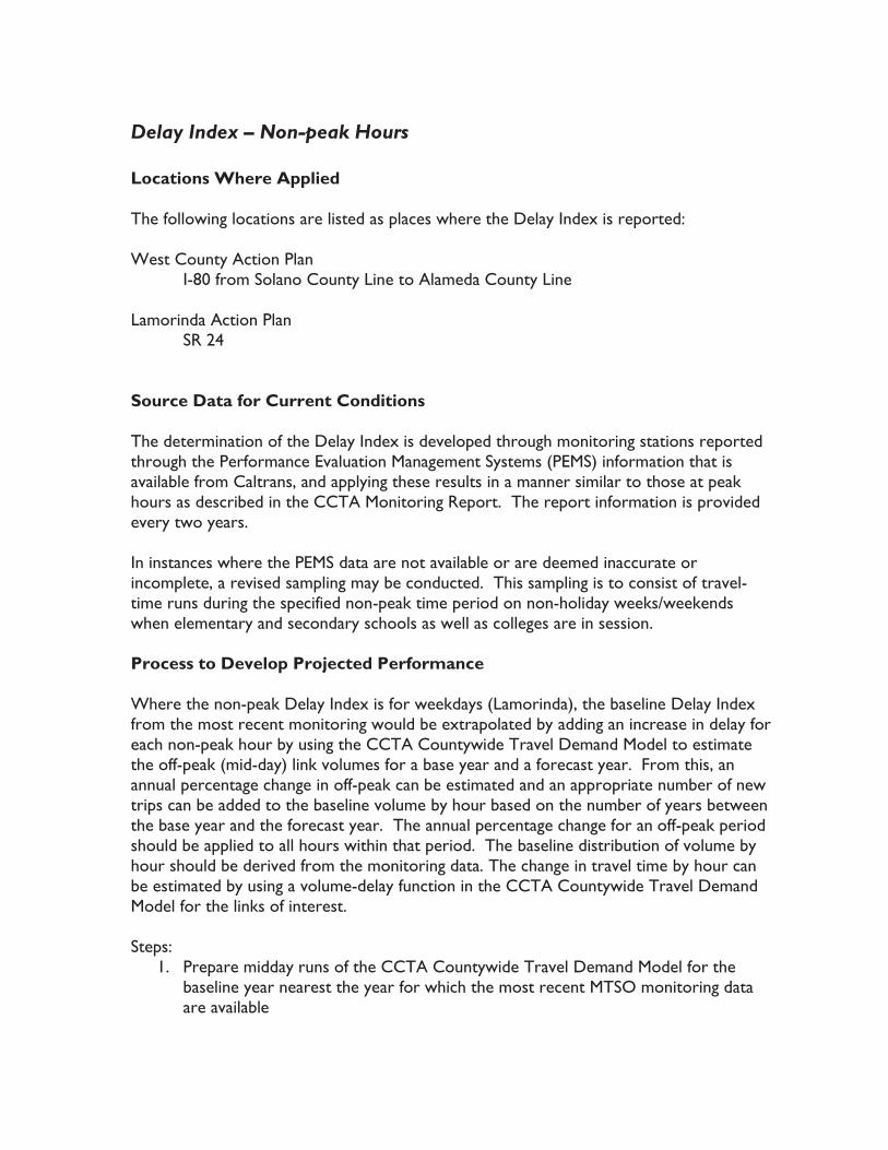
Delay Index – Non-peak Hours Locations Where Applied The following locations are listed as places where the Delay Index is reported: West County Action Plan
I-80 from Solano County Line to Alameda County Line Lamorinda Action Plan
SR 24 Source Data for Current Conditions The determination of the Delay Index is developed through monitoring stations reported through the Performance Evaluation Management Systems (PEMS) information that is available from Caltrans, and applying these results in a manner similar to those at peak hours as described in the CCTA Monitoring Report. The report information is provided every two years. In instances where the PEMS data are not available or are deemed inaccurate or incomplete, a revised sampling may be conducted. This sampling is to consist of travel-time runs during the specified non-peak time period on non-holiday weeks/weekends when elementary and secondary schools as well as colleges are in session. Process to Develop Projected Performance Where the non-peak Delay Index is for weekdays (Lamorinda), the baseline Delay Index from the most recent monitoring would be extrapolated by adding an increase in delay for each non-peak hour by using the CCTA Countywide Travel Demand Model to estimate the off-peak (mid-day) link volumes for a base year and a forecast year. From this, an annual percentage change in off-peak can be estimated and an appropriate number of new trips can be added to the baseline volume by hour based on the number of years between the base year and the forecast year. The annual percentage change for an off-peak period should be applied to all hours within that period. The baseline distribution of volume by hour should be derived from the monitoring data. The change in travel time by hour can be estimated by using a volume-delay function in the CCTA Countywide Travel Demand Model for the links of interest. Steps:
1. Prepare midday runs of the CCTA Countywide Travel Demand Model for the baseline year nearest the year for which the most recent MTSO monitoring data are available

2. Estimate the congested travel time for the route of regional significance summing the congested travel times for all the mixed-flow lane links of the route
3. Prepare midday runs of the CCTA Countywide Travel Demand Model for the available future year closest to the forecast year and for a network reflecting Action Plan projects
4. Estimate the congested travel time for the route of regional significance summing the congested travel times for all the mixed-flow lane links of the route
5. Subtract the congested route travel time for the baseline year form the value for the forecast year and divide by the number of years separating the two forecast years to get an estimate of the annual increase in congested travel time for the route.
6. Multiply the average annual increase in congested route travel time by the number of years between the most recent MTSO monitoring data and the forecast year and add this increment of travel time to the MSTO monitoring value.
7. Divide the estimate of future year congested travel time to the estimate of uncongested travel time for the route that was used in the most recent monitoring report to get the new forecast-year estimate of Delay Index for the route.

Duration of Congestion Locations Where Applied Tri Valley
I-680 SR 84
Source Data for Current Conditions The estimate for “duration of congestion” should be based on monitoring stations reported through the Performance Evaluation Management Systems (PEMS) information that is available from Caltrans and reported in the most recent CCTA Monitoring Report. The report information is provided every two years. In instances where the Monitoring Report is deemed inaccurate or incomplete and PEMS data are not available, a revised sampling may be conducted. This sampling is to consist of travel-time runs during the hours of 6 A.M. and 7 P.M. The sampling should be made on a Tuesday, Wednesday or Thursday on non-holiday weeks when elementary and secondary schools as well as colleges are in session. An average operating speed for the mixed-flow lanes of each segment should be developed for each half-hour period. A congested half-hour is one that has an average operating speed of 35 miles peer hour or less or the segment exceeds the delay-index target if one exists. Process to Develop Projected Performance Forecasts of average operating speed by half-hour period for each segment of interest should be developed by using forecasts from the CCTA Countywide Travel Demand Model. The baseline operating speeds from the most recent monitoring would be extrapolated by adding an increase in travel time for each hour by using the CCTA Countywide Travel Demand Model to estimate the peak and off-peak (mid-day) link volumes) for a base year and a forecast year. From this, an annual percentage change in volume for each half-hour period of interest can be estimated using either the percentage change for the Peak or the percentage change for the off-peak (mid-day) and an appropriate number of new trips can be added based on the number of years between the base year and the forecast year. The change in speed can be estimated by using a volume-delay function in the CCTA Countywide Travel Demand Model for the links of interest. Steps:
1. Prepare AM and PM peak period runs of the CCTA Countywide Travel Demand Model for the baseline year nearest the year for which the most recent MTSO monitoring data are available
2. Estimate the congested travel time for the route of regional significance summing the congested travel times for all the mixed-flow lane links of the route to get the total vehicle hours of travel

3. Multiple the volumes on each link by the length of the link to get the total vehicle miles of travel by link.
4. Sum the VMT by link over all of the mixed flow lanes for the length of the route to get the total VMT for the route.
5. Divide the total VMT for the route by the congested VHT for the route to get the average travel speed
6. Prepare midday runs of the CCTA Countywide Travel Demand Model for the baseline year nearest the year for which the most recent MTSO monitoring data are available
7. Estimate the congested travel time for the route of regional significance summing the congested travel times for all the mixed-flow lane links of the route to get the total vehicle hours of travel
8. Multiple the volumes on each link by the length of the link to get the total vehicle miles of travel by link.
9. Sum the VMT by link over all of the mixed flow lanes for the length of the route to get the total VMT for the route.
10. Divide the total VMT for the route by the congested VHT for the route to get the average travel speed
11. Prepare midday runs of the CCTA Countywide Travel Demand Model for the available future year closest to the forecast year and for a network reflecting Action Plan projects

Volume-Capacity Ratio Locations Where Applied Tri Valley
SR 84 Source Data for Current Conditions Volume-Capacity Ratio is the ratio of traffic volume to the capacity of the roadway. The volume Capacity Ratio can be monitored by observing the traffic volumes at key points or links being analyzed. The traffic volume is then divided by the operational capacity of the roadway of interest for the length of the peak-period specified. The capacity of each roadway link is available in the network description for each model year in the CCTA Countywide Travel Demand Model. Process to Develop Projected Performance Volume-Capacity Ratio for a future analysis year can be calculated by using the CCTA Countywide Travel Demand Model to get link assignment volumes for the forecast year and for the baseline year for which traffic count data are available. The differences (i.e. growth) in link volumes are then added to the traffic count data to estimate the traffic volume for the forecast year. This estimate of future-year volume is then divided by the hourly-capacity of the roadway multiplied by the number of hours in the peak-period being analyzed. Steps:
1. Prepare AM and PM peak period networks of the CCTA Countywide Travel Demand Model for the baseline year nearest the year for which the most recent MTSO monitoring data are available.
2. Prepare AM and PM peak period networks of the CCTA Countywide Travel Demand Model for the future year.
3. Subtract the volumes for each peak period between the future and base year to determine the anticipated traffic growth by the designated horizon year. If the base year traffic data does not match the future year data, some factoring of the anticipated growth may be necessary.
4. Apply the anticipated traffic growth to counts from the most recent MTSO monitoring program to determine the estimated volumes.
5. Determine capacity based upon lane capacity and number of lanes listed in the prior MTSO exercise for a representative segment of roadway.
6. Divide the projected, adjusted travel model volumes by the capacity calculated on the representative segment to determine the volume-capactiy ratio.

Mode Split Locations Where Applied Tri Valley Source Data for Current Conditions Mode split is the percentage of peak-period travelers that use transit as the mode of travel. Mode split is generally measured through extensive home interview and work place surveys. Information on commute trip mode share is also available every decade from the U.S. Census. Between decennial Census counts, transit ridership may be monitored, and changes in transit ridership may be used to update decennial mode splits. Process to Develop Projected Performance Peak-period Mode Split for future forecast years can be estimated using the CCTA Countywide Travel Demand Model. The model produces mode-specific person trip tables. These person trip tables may be summed on origins or summed on destinations for specific zone groups (e.g. an Action Plan area). The Mode Split MTSO can be estimated by dividing the total number of transit person trips by the total number of person trips (all modes) for a pre-specified set of TAZs. If mode split forecasts are available from the CCTA model for both the baseline year (for which monitoring data are available) and for the future forecast year, then the change in transit Mode Split can be applied to the baseline monitoring value to more reliably estimate future-year mode splits.
Steps:
1. Prepare runs of the CCTA Countywide Travel Demand Model for the future year.
2. Prepare tables showing total number of person trips, grouped for the TAZs in the specific study area.
3. Prepare tables showing total number of transit person trips, grouped for the TAZs in the specific study area.
4. Divide the total number of transit person trips by the total number of person trips to calculate the future year mode share.
5. If alternative sources are available from monitoring efforts or other reasons (such as household surveys), prepare the CCTA Countywide Travel Demand Model for the baseline year nearest the year for which the most recent MTSO monitoring data are available.
6. If Step 5 is undertaken, then calculate the model base year mode share by dividing the total number of transit person trips by the total number of person trips to calculate the base year mode share.
7. If Step 5 is undertaken, then apply the change in percentage between the base and future years to calculate anticipated future mode shares.

Average Vehicle Ridership Locations Where Applied Tri Valley Source Data for Current Conditions This MTSO is the ratio of total person commute trips to vehicles used for commuting. Average Vehicle Ridership is generally measured through extensive home interview and/or work place surveys. Information on commute trip mode share is also available every decade from the U.S. Census. Average Vehicle Ridership can be estimated from the Census data. Process to Develop Projected Performance Average Vehicle Ridership for commute trips for a future forecast year can be estimated using the CCTA Countywide Travel Demand Model. The model provides estimates of person trips by mode from or to a specified set of zones. The Average Vehicle Ridership is estimated by dividing the total number of person trips by the number of vehicle used for those trips. The number of vehicles used can be estimated by applying average vehicle occupancy for each mode. For the Tri-Valley the following average occupancies have been used:
Drive Alone 1 person per vehicle Shared Ride 2 2 people per vehicle Shared Ride 3 3.5 people per vehicle Transit No vehicle is included in the calculation
By developing the estimates of person trip by mode from all of the zones within the area covered by the MTSO, an estimate of the Average Vehicle Ridership of residents commuting from the area can be developed. By developing an estimate of person trips by mode to all zones in the area of interest, an estimate of the Average Vehicle Ridership of trip makers employed in the area can be developed. If these estimates are developed for the baseline year for which monitoring data are available and for the future forecast year, the difference in Average Vehicle Ridership can be added to the baseline monitoring value to get the forecast year value for the MTSO.
Steps:
1. Prepare runs of the CCTA Countywide Travel Demand Model for the future year.
2. Prepare tables showing total number of person trips, grouped for the TAZs in the specific study area.
3. Prepare tables showing total number of person trips by each mode (drive alone, two-person vehicles, three or more person vehicles, and transit riders), grouped for the TAZs in the specific study area.

4. Calculate the number of vehicle trips for each mode -- by dividing the two-person carpool totals by 2, and the three-or-more person carpools by 3.5, (Drive-alone person trips and vehicle trips are the same number).
5. Sum the total number of vehicles by adding the number of drive-alone vehicle/person trips, the number of vehicles in two-person carpools, and the number of persons in three-or-more-person carpools.
6. Calculate the Average Vehicle Occupancy by dividing the total number of person trips by the total number of vehicle trips for the future year.
7. If alternative sources are available from monitoring efforts or other reasons (such as household surveys), prepare the CCTA Countywide Travel Demand Model for the baseline year nearest the year for which the most recent MTSO monitoring data are available.
8. If Step 7 is undertaken, then calculate the model base year average vehicle occupancy as outlined in steps 2 through 6.
9. If Step 7 is undertaken, then apply the change in percentage between the base and future years to calculate anticipated future average vehicle occupancy.

Average Speed Locations Where Applied Central County
Alhambra Avenue Clayton Road Contra Costa Boulevard Pacheco Boulevard Pleasant Hill Road Taylor Boulevard
Tri-Valley I-680 I-580
Source Data for Current Conditions Estimating average vehicular speeds for selected roadways is similar to computing the Delay Index in that both MTSOs are based on segment or route travel times. Average vehicular speeds and segment length (or distance) can be extracted from Caltrans’ Performance Evaluation Management Systems (PEMS) website. The report information is provided every two years. Arterial Roadways are not part of the PEMS system. In these cases, the current conditions should be measured as described in the CCTA Monitoring Report. The report information is provided every two years. Process to Develop Projected Performance The projected performance of the aver travel time may be calculated by adding the forecasted additional congested travel time that is expected to occur on the link to the current condition. This estimation is possible by using the loaded networks from the CCTA Countywide Travel Demand Model during peak hours, which contain a congested speed estimate for each link. This estimate of congested time by link may be summed for the mixed-flow lanes of the route for the nearest base year (such as 2010) and for the horizon year or year of completion (such as 2020 or 2030). The differences in summations would then be divided by the number of years between the forecasts (such as 10 or 20 years) for an annual forecast increase in travel time. This additional travel time would then be applied to the base-year monitoring results (annual travel-time increase multiplied by the number of years) to determine if the project impact would be significant at the compliance horizon year. Steps:
1. Prepare AM and PM peak-period runs of the CCTA Countywide Travel Demand Model for the baseline year nearest the year for which the most recent MTSO monitoring data are available.

2. Estimate the congested travel time for the route of regional significance by summing the congested travel times for all the mixed-flow lane links of the route.
3. Prepare AM and PM peak-period runs of the CCTA Countywide Travel Demand Model for the available future year closest to the forecast year and for a network reflecting Action Plan projects.
4. Estimate the congested travel time for the route of regional significance summing the congested travel times for all the mixed-flow lane links of the route
5. Subtract the congested route travel time for the baseline year from the value for the forecast year and divide by the number of years separating the two modeled years to get an estimate of the annual increase in congested travel time for the route.
6. Multiply the average annual increase in congested route travel time by the number of years between the most recent MTSO monitoring data and the forecast year and add this increment of travel time to the MSTO monitoring value.
7. Divide the estimate of future year congested travel time to the estimate of uncongested travel time for the route that was used in the most recent monitoring report.
8. Divide the resulting travel time by the segment distance to determine the average congested speed.

Vehicles in HOV Lane Locations Where Applied East County
State Route 4 West County I-80 Source Data for Current Conditions The HOV volumes reported in this MTSO are determined from the HOV lane utilization report published by Caltrans District 4. Process to Develop Projected Performance Future HOV-lane utilization may be calculated by adding the forecasted additional vehicles that are expected to use the HOV lane to the observed current HOV utilization. This estimation is possible by extracting peak-hour or peak-period HOV volumes from the CCTA Countywide Travel Demand Model loaded networks. The growth in HOV utilization would then be divided by the number of years between the forecasts (such as 10 or 20 years) for an annual forecast increase in HOV volumes. This additional annual volume would then be applied to the base-year monitoring results (volumes multiplied by the number of years) to determine if the project impact would be significant at the compliance horizon year. Steps:
1. Determine number of vehicles from most recent HOV performance report. (Note that Caltrans produces peak hour volume reports annually.)
2. Prepare AM and PM peak-hour assignments of the CCTA Countywide Travel Demand Model for the baseline year nearest the year for which the most recent MTSO monitoring data are available.
3. Prepare AM and PM peak-hour assignments of the CCTA Countywide Travel Demand Model for the available future year closest to the forecast year and for a network reflecting Action Plan projects.
4. Obtain the number of vehicles listed in the HOV lane from the model, using a representative link segments in the model, determined by finding the maximum volume on a link in the base year.
5. Determine an annual increase in HOVs from the base to the future year by dividing the number of additional vehicles by the number of years between the assignments.
6. Determine the actual HOV utilization by adding the change in Step 5 to the number of vehicles in Step 1.
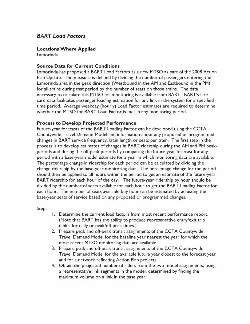
BART Load Factors Locations Where Applied Lamorinda Source Data for Current Conditions Lamorinda has proposed a BART Load Factors as a new MTSO as part of the 2008 Action Plan Update. The measure is defined by dividing the number of passengers entering the Lamorinda area in the peak direction (Westbound in the AM and Eastbound in the PM) for all trains during that period by the number of seats on those trains. The data necessary to calculate this MTSO for monitoring is available from BART. BART’s fare card data facilitates passenger loading estimation for any link in the system for a specified time period. Average weekday (hourly) Load Factor estimates are required to determine whether the MTSO for BART Load Factor is met in any monitoring period. Process to Develop Projected Performance Future-year forecasts of the BART Loading Factor can be developed using the CCTA Countywide Travel Demand Model and information about any proposed or programmed changes in BART service frequency, train length or seats per train. The first step in the process is to develop estimates of changes in BART ridership during the AM and PM peak-periods and during the off-peak-periods by comparing the future-year forecast for any period with a base-year model estimate for a year in which monitoring data are available. The percentage change in ridership for each period can be calculated by dividing the change ridership by the base-year monitoring data. The percentage change for the period should then be applied to all hours within the period to get an estimate of the future-year BART ridership for each hour of the day. The future-year ridership by hour should be divided by the number of seats available for each hour to get the BART Loading Factor for each hour. The number of seats available buy hour can be estimated by adjusting the base-year seats of service based on any proposed or programmed changes. Steps:
1. Determine the current load factors from most recent performance report. (Note that BART has the ability to produce representative entry/exit trip tables for daily or peak/off-peak times.)
2. Prepare peak and off-peak transit assignments of the CCTA Countywide Travel Demand Model for the baseline year nearest the year for which the most recent MTSO monitoring data are available.
3. Prepare peak and off-peak transit assignments of the CCTA Countywide Travel Demand Model for the available future year closest to the forecast year and for a network reflecting Action Plan projects.
4. Obtain the projected number of riders from the two model assignments, using a representative link segments in the model, determined by finding the maximum volume on a link in the base year.

5. Determine an annual increase in transit riders from the base to the future year by dividing the number of additional riders by the number of years between the assignments.
6. Determine the adjusted, projected number of riders by adding the change in Step 5 to the number of vehicles in Step 1.
7. Determine the number of seats in the current condition during peak and off-peak periods by multiplying the number of bart seats per car by the number of cars during the peak period (with the number of cars potentially estimated by the number of trains multiplied by the number of cars per train).
8. Determine the percentage increase in the number of trains assumed in the peak and off-peak transit networks for the base and future years by comparing the train headways in the model. (Model headways are typically the inverse of the number of trains.)
9. Multiply the capacity increase percentage in Step 8 by the number of seats in Step 7.
10. Divide the number of adjusted, projected number of riders in Step 6 by the capacity in Step 9. (It is acceptable to have more riders than seats).

Minimum Bus Frequency Locations Where Applied Lamorinda
Pleasant Hill Road Source Data for Current Conditions Lamorinda has proposed a Minimum Bus Frequency on Pleasant Hill road as a new MTSO as part of the 2008 Action Plan Update. The measure is defined as the composite number of buses per direction per hour for all routes serving the corridor between Taylor Blvd and Acalanes High School during peak commute and school times (6:30 AM – 9:30 AM and 3:30 PM – 6:30 PM). There is currently no bus service on Pleasant Hill Road. In the future monitoring can be performed by simply extracting peak-period headways from published bus schedules. Process to Develop Projected Performance Future-year forecasts of this MTSO can be developed using the increment method, whereby the number of hourly directional buses (for all routes) for all proposed new transit services are added to the MTSO’s baseline value.
Steps:
1. Determine the bus frequency from most recent bus schedules. (No service is provided in 2008.)
2. Compare transit peak-period headways in the CCTA Countywide Travel Demand Model for the available base year close to the monitoring year, and an available future year closest to the forecast year and for a network reflecting Action Plan projects. (The base year has no service coded in the Model.)
3. Determine the change in the number of buses (if any) between the base year and future year.
4. Apply the change in headways to the current bus frequency from the most recent bus schedules (if any service is provided) to calculate the projected bus frequency, and compare to the MTSO to determine if the minimum is achieved.

Side-street Wait Time Locations Where Applied Lamorinda
Pleasant Hill Road San Pablo Dam Road/Camino Pablo
Source Data for Current Conditions The Action Plan for Camino Pablo and San Pablo Dam Road includes a TSO specifying the maximum side-street wait time for vehicles waiting to access San Pablo Dam Road cannot exceed one cycle length. In the 2008 Action Plan Update, Lamorinda has also proposed that this MTSO be applied to Pleasant Hill Road. The measure is monitored through on-site observations. For future-year MTSO forecasting, base-year peak-period turning-movement counts are required at each study intersection where MTSO monitoring was performed. Process to Develop Projected Performance Intersection Level of Service analysis procedures are described in Chapter 4 and Appendix C of the Technical Procedures. Turning-movement traffic volumes for the routes of regional significance and their side-street approaches should be forecasted using the CCTA Countywide Travel Demand Model. The increment method should be used to estimate future turning-movement volumes to be used in the intersection LOS analysis, whereby model-estimated growth in turning-movement volumes are added to counted baseline turning-movement volumes. The intersection LOS procedure should be used to determine whether the intersection threshold level of service can be achieved while providing sufficient green time to meet side-street demand at least 95% of the time during the peak commute hours. Steps:
1. Prepare peak and off-peak transit assignments of the CCTA Countywide Travel Demand Model for the baseline year nearest the year for which the most recent MTSO monitoring data are available.
2. Prepare peak and off-peak transit assignments of the CCTA Countywide Travel Demand Model for the available future year closest to the forecast year and for a network reflecting Action Plan projects.
3. Utilize the CCTA intersection turning movement adjustment method to calculate future traffic volumes.
4. Utilize the intersection LOS determination procedure to determine whether or not the volume-capacity ratio is less than 1.0. (If it is, then it can be anticipated that the side street wait time would remain within a minimum delay threshold.)
5. For intersections which are near or above 1.0, perform a more detailed intersection LOS study. The intersection delay be approach would then be examined for delays from the side street approaches.

West County Area-wide Goals A number of area-wide goals have been developed for the West County Action Plan. These goals represent items which are to be monitored by the CCTA when they measure the MTSOs every four years. These are baseline measures; forecasting future-year performance for these goals is not required. Steps: None Source Data for Transit Satisfaction Goal This area-wide goal is to be measured through the most recent transit operator rider surveys. Source Data for Pavement Quality Goal This is to be measured by comparing Agency-monitored Pavement Condition indices for each partner jurisdiction. Source Data for Drive-Alone Rate This area-wide goal of 75 percent is to be measured by field observation and/or vehicle occupancy surveys. The measurement is typically taken on Interstate 580 near the Alameda County line. Source Data for Transit Ridership Increase This increase of 10 percent between 2007 and 2012 is to be measured by comparing AC Transit, WestCAT and BART boarding data in West County in those two years. Source Data for Bicycle and Pedestrian Mode Share The goal of 3 percent is to be monitored by using the American Community Survey responses concerning transportation mode percentages in 2012. Source Data for Capitol Corridor Daily Ridership The goal of 3,000 riders a day would be measured by collecting ridership data. The data is based on the number of riders traveling through Contra Costa County between Richmond and Martinez stations in 2012. (NOTE: DKS unable to verify how this is determined.) Source Data for Ferry Service Daily Ridership The proposed ferry service for Richmond-San Francisco and Hercules-San Francisco has goals of 500 passengers per day each by 2012. These would be measured by examining weekday boardings for each route in 2012. Source Data for On-time Bus Transit Performance This new goal is to be measured by comparing AC Transit, WestCAT and BART data in West County according to the on-time performance definitions of the various systems.

The goal is to maintain 2007 on-time performance levels. (DKS note: BART on-time performance is “rail” and not “bus”.)

Average Intersection Stopped Delay Locations Where Applied 6 Central County Intersections in Concord Source Data for Current Performance The MTSO is defined as stopped delay, but the measurement is made through the number of signal cycles needed to clear the intersection. This is determined through the most recent CCTA Monitoring Report for both the AM and PM peak hours. Process to Develop Projected Performance Using HCM intersection analysis methods, the cycles needed to clear the intersection would be calculated by replicating the current delay using an HCM-consistent program. The procedures are then guided by the method established in the future year Intersection Level of Service process established by CCTA. Baseline and future-year peak-period (or peak hour) traffic volumes can be extracted from the CCTA Countywide Travel Demand Model for the routes of regional significance and side streets. The increment method should be used to estimate future turning-movement volumes to be used in the HCM intersection analysis, whereby the model-estimated growth in turning-movement volumes is added to counted baseline turning-movement volumes. Steps:
1. Prepare peak and off-peak transit assignments of the CCTA Countywide Travel Demand Model for the baseline year nearest the year for which the most recent MTSO monitoring data are available.
2. Prepare peak and off-peak transit assignments of the CCTA Countywide Travel Demand Model for the available future year closest to the forecast year and for a network reflecting Action Plan projects.
3. Utilize the CCTA intersection turning movement adjustment method to calculate future traffic volumes.
4. Utilize the intersection LOS determination procedure to determine the average stopped delay.


Appendix B - Traffic Counting Protocol


Appendix B TRAFFIC COUNTING PROTOCOL
Traffic counts for traffic impact studies, level of service monitoring, and any other application intended to represent prevailing traffic conditions at a given location shall be conducted in accordance with the following provisions:
aa. During Fair Weather – Counts shall be conducted in fair weather, without rain, flooding, heavy winds, or other adverse weather conditions that could disrupt the flow of traffic;
b. On Tuesday, Wednesday, or Thursday of a non-holiday week when public schools are in session – Holidays include New Years Day, Martin Luther King Day, President’s Day, Memorial Day, Independence Day, Labor Day, Veteran’s Day, Thanksgiving, and Christmas.
c. Typical School Day –Counts should be taken on typical school days avoiding half days, late start days and early-dismissal days whenever possible.
d. No major road closings – if temporary road closings have occurred that affect traffic flow at the count location, the count should be postponed until the road is re-opened. If the road closing is to be for an extended period, and a count needs to be conducted, the count results should be annotated to reflect the road closure conditions.
e. No construction activity – Counts should not be conducted in the presence of construction activity that could disrupt the arrival or departure of traffic at the count location.
f. No incidents or accidents – If an incident or accident has occurred in the vicinity of the count location, or if such an event occurs during the count, the count should be discarded, and repeated at a later date.
In the event that a traffic count is conducted specifically to observe conditions under provisions a-f above, the prevalence of such condition(s) should be duly noted in any documents or data that are used to report the count results.


Appendix C - Guidelines for Use of the 2010 Highway Capacity Manual Operational Method Methodology


Appendix C – Guidelines for the Use of the 2010 Highway Capacity Manual Operational Method Methodology
Purpose of the Guidelines To ensure consistency in the application of the 2010 Highway Capacity Manual operational method for assessment of signalized intersections in Contra Costa, guidelines have been developed for the way in which the method is to be applied. The guidelines include when location-specific data should be used, the specific values to be used for parameters when location-specific values are not used, and the type of documentation to be provided. These guidelines are not intended to be instructions for how to use the 2010 Highway Capacity Manual operational method. Instructs are provided in Chapter 18 of the 2010 Highway Capacity Manual. The method should only be applied by someone trained in its use and preferably by a registered professional traffic engineer.
Documentation of Application When the 2010 Highway Capacity Manual operational method is used for any official review by the Contra Costa Transportation Authority or any of its member agencies, a description of the application must be provided. The description should document the following:
Date of the Analysis Name and Affiliation of the Analyst Time Frame for the Analysis – Existing Condition or Future Condition (specify year) Location Sources of Input Traffic Data and any other Location-Specific Data All Input Values (including default values) All Output
This information may be provided in a tabular form or as products from the software package used for the LOS analysis. A separate text report is not required for this documentation.
Parameters and Defaults Table 1 provides a comprehensive list of the data-input requirements of the 2010 Highway Capacity Manual operational method. Many of these input items are specific to an intersection and must be provided by the analysis from local data. They are as follows:
Traffic Characteristics
Demand Flow Rate (intersection turning movement volumes by movement) Initial Queue Pedestrian Flow Rate Bicycle Flow Rate

Geometric Design
Number of Lanes Number of Receiving lanes
Signal Control
Type of Signal Control Phase Sequence Left-turn Operational Mode
Other Characteristics
Speed limit Area Type
For all other input data items, Table 1 provides a value that should be used unless local information is available to use instead of the default value. As a supplement to Table 1, Table 2 provides default values for “Platoon Ratio” and Table 3 provides default values for “Base Saturation Flow Rate”. Table 1 indicates when the default values should be used and when a locally–derived value would be permissible. This may vary depending on whether the application is for a near-term year (existing condition or less than five years in the future) or a long-term year (forecast year greater than five years out). Almost all of the default values in Table 1 are provided in the 2010 Highway Capacity Manual – pages 18-74 through 18-78. The exception is for “Base Saturation Flow Rate”. The default values for this parameter, provided in Table 3, are taken from the Santa Clara Valley Transportation Authority’s “Traffic Level of Service Analysis Guidelines.” These values provide more detailed guidance by providing values for specific types of lanes and uses data from the Bay Area to support the defaults.

Data
Cat
egor
yIn
put D
ata
Elem
ent
Basi
sDe
faul
t Val
ues
Exist
ing
Cond
ition
s Nea
r-te
rm H
orizo
nLo
ng-t
erm
Hor
izon
(gre
ater
than
5 y
ears
)
Traf
fic
Char
acte
ristic
sDe
man
d flo
w ra
teM
ovem
ent
Use
r mus
t pro
vide
Use
r mus
t alw
ays s
peci
fy --
no
defa
ult v
alue
s for
tr
affic
vol
umes
Use
r mus
t alw
ays s
peci
fy --
no
defa
ult v
alue
s fo
r tra
ffic
volu
mes
Righ
t-tu
rn-o
n-re
d flo
w ra
teAp
proa
ch0.
0 ve
h/h
Use
r may
spec
ify --
if R
TOR
coun
ts w
ere
colle
cted
Use
sam
e as
Exi
stin
g Co
nditi
ons -
- or p
re-
appr
oval
by
CCTA
staf
f req
uire
dPe
rent
hea
vy v
ehic
les
Mov
emen
t gr
oup
3%U
ser m
ay sp
ecify
-- if
veh
icle
cla
ssifi
catio
n co
unts
wer
e co
llect
edU
se sa
me
as E
xist
ing
Cond
ition
s -- o
r pre
-ap
prov
al b
y CC
TA st
aff r
equi
red
Inte
rsec
tion
peak
hou
r fac
tor
Inte
rsec
tion
If an
alys
is pe
riod
is 0.
35 h
and
ho
urly
dat
a ar
e us
ed:
Tota
l ent
erin
g vo
lum
e >
1,00
0 ve
h/h:
0.9
2To
tal e
nter
ing
volu
me
< 1,
000
veh/
h: 0
.90
Use
r may
spec
ify --
if su
ffici
ent c
ount
dat
a w
ere
colle
cted
to g
et re
liabl
e pe
akin
g fa
ctor
sU
se sa
me
as E
xist
ing
Cond
ition
s -- o
r pre
-ap
prov
al b
y CC
TA st
aff r
equi
red
Plat
oon
ratio
Mov
emen
t gr
oup
See
Tabl
e 2
Use
r may
spec
ify --
if su
ffici
ent c
ount
dat
a w
ere
colle
cted
to g
et re
liabl
e ra
tioU
se sa
me
as E
xist
ing
Cond
ition
s -- o
r pre
-ap
prov
al b
y CC
TA st
aff r
equi
red
Ups
trea
m fi
lterin
g ad
just
men
t fa
ctor
Mov
emen
t gr
oup
1.0
Use
r may
spec
ify --
if su
ffici
ent c
ount
dat
a w
ere
colle
cted
to g
et re
liabl
e fa
ctor
Use
sam
e as
Exi
stin
g Co
nditi
ons -
- or p
re-
appr
oval
by
CCTA
staf
f req
uire
dIn
itial
que
ueM
ovem
ent
grou
pU
ser m
ust p
rovi
deU
ser m
ust a
lway
s spe
cify
-- n
o de
faul
t val
ues f
or
traf
fic v
olum
esU
se sa
me
as E
xist
ing
Cond
ition
s -- o
r fa
ctor
ed b
ased
on
fore
cast
ed g
row
th in
ap
proa
ch tr
affic
vol
umes
Base
satu
ratio
n flo
w ra
teM
ovem
ent
grou
p1,
900
pc/h
/InAl
mos
t alw
ays u
ser s
houl
d us
e de
faul
t val
ues -
- un
less
a sa
t flo
w ra
te st
udy
was
per
form
ed,
revi
ewed
and
app
rove
d by
CCT
A st
aff.
Use
sam
e as
Exi
stin
g Co
nditi
ons -
- or p
re-
appr
oval
by
CCTA
staf
f req
uire
d
Lane
util
izatio
n ad
just
men
t fac
tor
Mov
emen
t1.
0U
ser m
ay sp
ecify
-- if
indi
vidu
al la
ne c
ount
dat
a w
ere
colle
cted
to g
et re
liabl
e la
ne u
tiliza
tion
fact
ors
Use
sam
e as
Exi
stin
g Co
nditi
ons -
- or p
re-
appr
oval
by
CCTA
staf
f req
uire
d
Pede
stria
n flo
w ra
teAp
proa
chU
ser m
ust p
rovi
deU
ser m
ust s
peci
fyU
se sa
me
ped
flow
rate
s as E
xist
ing
Cond
ition
s, o
r fac
tore
d ba
sed
on lo
cal l
and
use
grow
th fo
reca
sts.
Bicy
cle
flow
rate
Appr
oach
Use
r mus
t pro
vide
Use
r mus
t spe
cify
Use
sam
e bi
ke fl
ow ra
tes a
s Exi
stin
g Co
nditi
ons,
or f
acto
red
base
d on
loca
l lan
d us
e gr
owth
fore
cast
s.
On-
stre
et p
arki
ng m
aneu
ver r
ate
Mov
emen
t gr
oup
0.0
unle
ss k
now
nU
ser m
ay sp
ecify
, if u
nkno
wn
use
"0"
Use
sam
e pa
rkin
g ac
tivity
rate
s as E
xist
ing
Cond
ition
s, o
r fac
tore
d ba
sed
on g
row
th in
tr
affic
vol
umes
Tabl
e 1
201
0 HC
M O
pera
tiona
l Met
hod
Inpu
t Dat
a Re
quire
men
ts a
nd R
ecom
men
ded
Defa
ult V
alue
s

Data
Cat
egor
yIn
put D
ata
Elem
ent
Basi
sDe
faul
t Val
ues
Exist
ing
Cond
ition
s Nea
r-te
rm H
orizo
nLo
ng-t
erm
Hor
izon
(gre
ater
than
5 y
ears
)Ta
ble
1 2
010
HCM
Ope
ratio
nal M
etho
d In
put D
ata
Requ
irem
ents
and
Rec
omm
ende
d De
faul
t Val
ues
Loca
l bus
stop
ping
rate
Appr
oach
Whe
n bu
ses e
xpec
ted
to st
opCe
ntra
l bus
ines
s dist
rict:
1
2 bu
ses/
hN
on-c
entr
al b
usin
ess d
istric
t: 2
buse
s/h
Whe
n bu
ses n
ot e
xpec
ted
to
stop
: 0
Use
r may
spec
ify, i
f unk
now
n us
e "0
"U
se sa
me
as E
xist
ing
Cond
ition
s -- o
r pre
-ap
prov
al b
y CC
TA st
aff r
equi
red
Geom
etric
De
sign
Num
ber o
f lan
esM
ovem
ent
grou
pU
ser m
ust p
rovi
deU
ser m
ust a
lway
s spe
cify
-- n
o de
faul
t val
ues f
or
num
ber o
f lan
esU
ser m
ust a
lway
s spe
cify
-- n
o de
faul
t val
ues
for n
umbe
r of l
anes
Aver
age
lane
wid
thM
ovem
ent
grou
p12
ftU
ser m
ay sp
ecify
-- if
lane
wid
ths a
re k
now
nU
ser m
ay sp
ecify
-- if
lane
wid
ths a
re k
now
n fo
r fut
ure
cond
ition
sN
umbe
r of r
ecei
ving
lane
sAp
proa
chU
ser m
ust p
rovi
deU
ser m
ust a
lway
s spe
cify
-- n
o de
faul
t val
ues f
or
num
ber o
f lan
esU
ser m
ust a
lway
s spe
cify
-- n
o de
faul
t val
ues
for n
umbe
r of l
anes
Turn
bay
leng
thM
ovem
ent
grou
pU
ser m
ust p
rovi
deU
ser m
ust s
peci
fy --
no
defa
ult v
alue
sU
ser m
ust s
peci
fy --
no
defa
ult v
alue
s
Pres
ence
of o
n-st
reet
par
king
Mov
emen
t gr
oup
Use
r mus
t pro
vide
Use
r may
spec
ify --
if p
arki
ng c
ondi
tions
are
kn
own
Use
sam
e as
Exi
stin
g Co
nditi
ons -
- or p
re-
appr
oval
by
CCTA
staf
f req
uire
dAp
proa
ch g
rade
Appr
oach
Flat
app
roac
h: 0
%M
oder
ate
grad
e on
apr
oach
: 3% St
eep
grad
e on
app
roac
h: 6
%
Use
r may
spec
ify --
if g
rade
at I
/S is
kno
wn
Use
sam
e as
Exi
stin
g Co
nditi
ons -
- or p
re-
appr
oval
by
CCTA
staf
f req
uire
d
Sign
al C
ontr
olTy
pe o
f sig
nal c
ontr
olIn
ters
ectio
n U
ser m
ust p
rovi
deU
ser m
ust s
peci
fyU
se sa
me
as E
xist
ing
Cond
ition
s -- o
r pre
-ap
prov
al b
y CC
TA st
aff r
equi
red
Phas
e se
quen
ceIn
ters
ectio
n U
ser m
ust p
rovi
deU
ser m
ust s
peci
fyU
se sa
me
as E
xist
ing
Cond
ition
s -- o
r pre
-ap
prov
al b
y CC
TA st
aff r
equi
red
Left
-tur
n op
erat
oina
l mod
eAp
proa
chU
ser m
ust p
rovi
deU
ser m
ust s
peci
fyU
se sa
me
as E
xist
ing
Cond
ition
s -- o
r pre
-ap
prov
al b
y CC
TA st
aff r
equi
red
Dalla
s lef
t-tu
rn p
hasin
g op
tion
Appr
oach
Dict
ated
by
loca
l use
Pass
age
time
(if a
ctua
ted)
Phas
e2.
0 s (
pres
ence
det
ectio
n)U
ser m
ay sp
ecify
-- if
kno
wn,
else
use
HCM
de
faut
val
ues
Use
sam
e as
Exi
stin
g Co
nditi
ons -
- or p
re-
appr
oval
by
CCTA
staf
f req
uire
dM
axim
um g
reen
(or g
reen
du
ratio
n if
pret
imed
)Ph
ase
Maj
or-s
tree
t thr
ough
m
ovem
ent:
50 s
Min
or-s
tree
t thr
ough
m
ovem
ent:
30 s
Left
-tur
n m
ovem
ent:
20 s
Use
r may
spec
ify --
if k
now
n, e
lse u
se H
CM
defa
ut v
alue
sU
se sa
me
as E
xist
ing
Cond
ition
s -- o
r pre
-ap
prov
al b
y CC
TA st
aff r
equi
red

Data
Cat
egor
yIn
put D
ata
Elem
ent
Basi
sDe
faul
t Val
ues
Exist
ing
Cond
ition
s Nea
r-te
rm H
orizo
nLo
ng-t
erm
Hor
izon
(gre
ater
than
5 y
ears
)Ta
ble
1 2
010
HCM
Ope
ratio
nal M
etho
d In
put D
ata
Requ
irem
ents
and
Rec
omm
ende
d De
faul
t Val
ues
Min
imum
gre
enPh
ase
Maj
or-s
tree
t thr
ough
m
ovem
ent:
10 s
Min
or-s
tree
t thr
ough
m
ovem
ent:
8 s
Left
-tur
n m
ovem
ent:
6 s
Use
r may
spec
ify --
if k
now
n, e
lse u
se H
CM
defa
ut v
alue
sU
se sa
me
as E
xist
ing
Cond
ition
s -- o
r pre
-ap
prov
al b
y CC
TA st
aff r
equi
red
Yello
w c
hang
ePh
ase
Yello
w c
hang
e +
Red
clea
ranc
e =
4.0
sU
ser m
ay sp
ecify
-- if
kno
wn,
else
use
HCM
de
faut
val
ues
Use
sam
e as
Exi
stin
g Co
nditi
ons -
- or p
re-
appr
oval
by
CCTA
staf
f req
uire
dRe
d cl
eara
nce
Phas
eYe
llow
cha
nge
+ Re
d cl
eara
nce
= 4.
0 s
Use
r may
spec
ify --
if k
now
n, e
lse u
se H
CM
defa
ut v
alue
sU
se sa
me
as E
xist
ing
Cond
ition
s -- o
r pre
-ap
prov
al b
y CC
TA st
aff r
equi
red
Wal
kPh
ase
Actu
ated
: 7.0
sPr
etim
ed: g
reen
inte
rval
min
us
pede
stria
n cl
ear
Use
r may
spec
ify --
if k
now
n, e
lse u
se H
CM
defa
ut v
alue
sU
se sa
me
as E
xist
ing
Cond
ition
s -- o
r pre
-ap
prov
al b
y CC
TA st
aff r
equi
red
Pede
stria
n cl
ear
Phas
eBa
sed
on 3
.5-ft
/s w
alki
ng
spee
dU
ser m
ay sp
ecify
-- if
kno
wn,
else
use
HCM
de
faut
val
ues
Use
sam
e as
Exi
stin
g Co
nditi
ons -
- or p
re-
appr
oval
by
CCTA
staf
f req
uire
dPh
ase
reca
llPh
ase
Actu
ated
pha
se: N
oPr
etim
ed p
hase
: Rec
all t
o m
axim
um
Use
r may
spec
ify --
if k
now
n, e
lse u
se H
CM
defa
ut v
alue
sU
se sa
me
as E
xist
ing
Cond
ition
s -- o
r pre
-ap
prov
al b
y CC
TA st
aff r
equi
red
Dual
ent
ry (i
f act
uate
d)Ph
ase
Not
ena
bled
(i.e
., us
e sin
gle
entr
y)U
ser m
ay sp
ecify
-- if
kno
wn,
else
use
HCM
de
faut
val
ues
Use
sam
e as
Exi
stin
g Co
nditi
ons -
- or p
re-
appr
oval
by
CCTA
staf
f req
uire
dSi
mul
tane
ous g
ap-o
ut (i
f ac
tuat
ed)
Appr
oach
Enab
leU
ser m
ay sp
ecify
-- if
kno
wn,
else
use
HCM
de
faut
val
ues
Use
sam
e as
Exi
stin
g Co
nditi
ons -
- or p
re-
appr
oval
by
CCTA
staf
f req
uire
dO
ther
Anal
ysis
perio
d du
ratio
nIn
ters
ectio
n 0.
25 h
Use
r mus
t use
def
ault
valu
eU
ser m
ust u
se d
efau
lt va
lue
Spee
d lim
itAp
proa
chU
ser m
ust p
rovi
deU
ser m
ay sp
ecify
if sp
eed
limits
are
kno
wn
(else
us
e 30
mph
)U
se sa
me
as E
xist
ing
Cond
ition
s -- o
r pre
-ap
prov
al b
y CC
TA st
aff r
equi
red
Stop
-line
det
ecto
r len
gth
and
dete
ctio
n m
ode
Mov
emen
t gr
oup
40 ft
(pre
senc
e de
tect
ion)
Use
r may
spec
ify if
det
ectio
n in
form
atio
n is
know
nU
se sa
me
as E
xist
ing
Cond
ition
s -- o
r pre
-ap
prov
al b
y CC
TA st
aff r
equi
red
Area
type
Inte
rsec
tion
Use
r mus
t pro
vide
Use
r mus
t spe
cify
Use
r mus
t spe
cify
Satu
ratio
n Fl
ow R
ate
Mov
emen
tSe
e Ta
ble
3U
ser m
ust u
se d
efau
lt va
lue
Use
r mus
t use
def
ault
valu
e
Sour
ce: H
ighw
ay C
apac
ity M
anua
l 201
0 pa
ge 1
8-75
.

Platoon Ratio Arrival Type Progression Quality0.33 1 Very Poor0.67 2 Unfavorable1.00 3 Random Arrivals1.33 4 Favorable1.67 5 Highly Favorable2.00 6 Exceptionally Favorable
Table 2 Default Values for Platoon Ratio

1 Lane 2 Lanes 3 Lanes 4 LanesLeft Turn 1750
(0.921053)3150
(0.828947)4550
(0.798421)Left Through 1800
(0.947368)Through 1900
(1.000000)3800
(1.000000)5700
(1.000000)7600
(1.000000)Right Through 1800
(0.947368)Right Turn 1750
(0.921053)3150
(0.828947)4550
(0.798421)Left Through Right 1750
(0.921053)
Source: SCVTA Traffic level of Service Analysis Guidelines 2003
Table 3 Default Saturation Flow Rates
Movement
Default Saturation Flow Rate (vph)(Default TRAFFIX Adjustment Factor)*
* In TRAFFIX =, saturation flow rates are specified through the use of adjustment factors to default idealsaturation flow rates.


Appendix D - Guidelines for Use of the CCTALOS Methodology


Appendix D CCTALOS Methodology
The CCTALOS methodology may be used to evaluate existing levels of service at signalized intersections using actual traffic count data, or future levels of service using forecast traffic projections. The Authority’s method is similar to the Circular 212 Planning Method except that through movement capacity has been increased from 1,500 vehicles per hour to 1,800 vehicles per hour. Level of service is calculated by critical movement with lower capacities assumed for turning movements.
SSaturation Flow Rates
The saturation flow rate is the basis for determining the capacity of an intersection. It represents the maximum number of vehicles that can pass through an intersection under prevailing traffic conditions. The Authority has modified the Circular 212 Operations and Design Method by assuming a saturation flow rate of 1,800 vehicles per hour (rather than 1,500 vehicles per hour).
Saturation flow rates were measured at four intersections in Contra Costa in February, 1990 to verify the appropriateness of this saturation flow rate. The method for collecting saturation flow rate data described in the 1985 Highway Capacity Manual (HCM) was used. The results are summarized in Table 1. Considerable variation in saturation flow rates were observed at each intersection. The data suggested that the operations and design capacities based on the 1,800 vehicles per hour saturation flow rate are frequently achieved within Contra Costa.
Table 1: Measured PM Peak Hour Saturation Flow Rates Selected Intersections in CContra Costa
Intersection Movement
Number of Samples
Highest Measured (Vehicles Per
Hour)
Treat Boulevard/Clayton Road
Left 4 1,752
Left/Thru 4 2,054
Thru 8 2,487
Thru/Right 4 1,793
Buchanan Road/Somersville Road
Left 8 2,048
Thru 2 2,014
Alcosta Drive/Crow Canyon Road
Left 3 2,152
Thru 5 2,261
Right 1 2,531

Blume Drive/HilltopDrive Left 4 2,084
Thru 4 1,807
WEIGHTED AVERAGE Left 19 2,152
Left/Thru 4 2,054
Thru 19 2,487
Thru/Right 4 1,793
Right 1 2,531
Source: Patterson Associates, February, 1990
As indicated in Table 1, the saturation flow rates varied by movement type. Exclusive left-turn saturation flow rates were approximately 10 percent less than those for through lanes. Saturation flow rates for shared left and through lanes were 18 percent lower than for through lanes. Sufficient data was not collected to provide statistical accuracy for these averages. They were consistent, however, with the passenger car equivalent (PCE) values adjustments provided in Circular 212.
Optional Capacity Reduction The effect of vehicle mix, intersection geometrics and other factors on intersection capacity is well documented. These factors, however, are not considered directly in the Circular 212 Planning Methodology. This was why a lower capacity (1,500 vph) was originally selected for use in Circular 212.
The Authority methodology, which uses a higher capacity (1,800 vph), may underestimate existing or future congestion at some locations. The reductions in the capacities provided in Table 2 are therefore optional, provided that measurement of saturation flow rates at those locations justify the lower capacities. Under no circumstances can a signalized intersection capacity above 1,800 vph be used under the Authority methodology. Saturation flow rates must be measured using the technique described in Section 9, Appendix IV of the 1985 Highway Capacity Manual.
Table 22: Lane Capacities1
Lane Type 2-Phase 3-Phase 4+-Phase
Exclusive Lane 1,800 1,720 1,650
Shared Lane 1,800 1,720 1,650
Dual Turn Lanes2,3 1,636 1,564 1,500
Triple Turn Lanes2,4 1,565 1,496 1,435 Capacities for a single lane. If multiple lanes are provided, capacity in the table is multiplied by number of lanes to obtain total capacity for movement group.
Can include one shared lane (e.g. one exclusive left, plus one shared through left is considered dual turn lane).
Assumes 45%–55% lane split.
Assumes lane use 15% higher in the most used lane.

The saturation flow rates be adjusted to establish the capacity for the traffic movement considered. Adjustment of the saturation flow rates should be performed as described in equation 9-1 of the 1985 HCM:
Cg x s = c
iii
Where (for lane group or approach i):
ci = capacity in vehicles per hour
si = saturation flow rate in vehicles per hour
g =effective green time in seconds
C =intersection cycle length in seconds
AAnalysis of Delay
Because the Authority’s LOS method applies fixed critical lane volumes uniformly throughout the county, the method may underestimate congestion at locations with poor geometrics (older intersections with poor turning radii and small approach widths), or overestimate congestion at locations with excellent geometrics (newer intersections with ideal conditions) and aggressive drivers. The Authority method may not identify locations where severe congestion is limited to a single intersection approach, nor does it reflect significant peaking and congestion within the peak hour.
To address these shortcomings, the following method may be used in lieu of the Authority’s method to identify congested locations:
Field measurement of delay on the congested approach or full intersection can be collected using the methodology described in the most recent version of the HCM. The measured delay should be compared with those provided in the most current version of the HCM.
Synchro® or similar software may be used in operations analyses to estimate vehicle delay and LOS based upon delay.
.V/C Level-of-Service Calculation Method
Signalized intersection levels of service may be calculated using the LOS software that is included “free” with this document, or a commercially-available software package that adheres to the Authority’s LOS methodology. The software incorporates the following steps. If done manually, the following nine steps should be used to perform the analysis:
Step 1 Lane Geometry
Identify the number and type of lanes for each approach.
Step 2 Intersection Volumes
Identify—by counting (if analyzing existing conditions) or estimating (if analyzing future conditions)—left-turn, through, and right-turn volumes for each approach for the peak (design) hour volumes in vehicles per hour for each peak hour to be analyzed. In most cases, the analysis will assess both the AM and PM weekday

peak hour. For projects with peak periods that occur during midday or on weekends, additional time periods should be analyzed.
SStep 3 Phasing
Identify the type of phasing (protected left turns, shared, or split) to be used at the intersection.
Step 4 Left-Turn Check
When a traffic signal phase permits left turns against opposing traffic rather than providing an exclusive left-turn phase, a check must be made to determine if sufficient left-turn capacity is provided to meet demand. This check will apply to LOS calculations for both existing, observed conditions and future estimated demand. Determination of the need for an exclusive left-turn phase under existing conditions should also consider actual traffic counts, left-turn delay, observed queuing, and accident history. The left-turn capacity is the combination of left turns made against opposing through movements and left turns made during the amber portion of the phase.
The capacity during the amber portion (VC)—the maximum number of left turns that can clear in this period—equals two times the number of signal cycles per hour. If the number of cycles per hour is not known, assume that the maximum number of left turns that can clear the intersection in one hour equals 90.
The capacity for left turns during the green cycle (VL)—the maximum number of left turns that can clear against opposing traffic volumes—is estimated using the following equation:
V - CG 1,200 = V OL
Where:
VL = left-turn volume, in vehicles per hour, that can clear during the green for opposing through traffic
G = maximum green plus amber time*
C = cycle time for opposing through traffic*
VO = sum of opposing through and right-turn volumes in vehicles per hour
* If either the maximum green time or the cycle time is not known, use the through and right-turn volumes for the approach divided by the number of lanes.
Add the number of left turns calculated in the change interval VC to the number calculated in the permitted left for a total number of left turns that can clear without a protected left (VL). If the number of left turns calculated above (left-turn capacity) is more than those estimated for the project, no protected left-turn phase is needed. If the number of left turns calculated above is less than the left turn demand, operating difficulties and increasing delays will be experienced.
Step 5 Adjust Turning Volumes
Two situations may require adjustment of observed or estimated turning volumes:
Right turns where no separate right-turn lane is provided and significant pedestrian activity exists, and
Left turns where no separate left-turn lane is provided.

The PCE adjustments recommended in Circular 212 should be used. If the Authority’s LOS software is used, adjustments to the turn volumes should be made prior to entering into the program.
SStep 6 Calculate Volume-to-Capacity Ratio by Movement
The volume-to-capacity ratio of each of the 12 individual movements and any combined movements of the intersection are calculated as follows:
Right-turn volumes on exclusive right-turn lanes are reduced to account for right turns on red. This reduction will equal the non-conflicting left-turn volumes with a minimum reduction of 90 vehicles per hour. (Non-conflicting left turns go concurrently with the right turn. For example, the non-conflicting left turn for the northbound right turn is the westbound left turn.) Determine the capacity of each movement and each combined movement from Table 2. Calculate the volume-to-capacity ratio for each movement and combined movement by dividing the adjusted volumes by the capacities. For combined movements, use the combined volumes divided by the combined capacities. Step 7 Determine Critical Volume-to-Capacity Ratios
Determine the highest total volume-to-capacity ratios for conflicting movements for both the north-south and east-west directions. For a non-split phased direction, the highest total of the right-turn or the through (or through plus right-turn if no exclusive right-turn lane exists) plus the opposing left-turn volume-to-capacity ratios are chosen. For a split phased direction, the highest volume-to-capacity ratio from each of the approaches is chosen. Free right turns are not included in the calculation since they are not under signal control.
Circular 212 does not clearly indicate how the critical movements are to be selected for single lane approaches (that is, when all right, left and thru movements are made from single approach lane). Under the Circular either the approach with the highest volume or both approaches could be designated as the critical movement. As part of the level-of-service method adopted by the Authority, however, both approaches should be considered critical movements.
Step 8 Sum the critical volume-to-capacity ratios for each approach
Step 9 Compare the sum of the critical volume-to-capacity ratio with the ranges in Table 3 to determine the intersection level of service

TTable 33:: Level of Service Ranges
Level of Service Sum of Critical V/C
A 0.60
B 0.61 - 0.70
C 0.71 - 0.80
D 0.81 - 0.90
E 0.91 - 1.00
F > 1.00
OOPTIONAL RIGHT-TURN ON RED ADJUSTMENT PROCEDURE
The VCCC method, as implemented in DOS, TransCAD, and other commercial software, internally reduces the input right turn volume, using the right turn lane code and other factors, to establish an “adjusted” volume that accounts for right turns on red (RTOR). The adjusted right-turn volume is then applied in the V/C calculation. This adjustment occurs automatically within the software, and is not directly controlled by the user.
Past experience has proven that, from time to time, the program does not adequately reflect higher levels of RTOR activity that may be occurring in the field. In cases where the program under-estimates the RTOR adjustment, it will also over-estimate the V/C ratio. If, in the analyst’s judgment, the RTOR adjustment is being underestimated, then the analyst has the option of conducting a RTOR count and further adjusting the right turn volumes used in the LOS computation based upon observed conditions.
The RTOR count may be conducted after the full turning movement count has been completed. The analyst should determine when the peak hour window occurred within the peak period of the full turning movement count, and should return to the intersection to conduct a spot count during that same peak hour window. The spot count should be for a minimum of one hour, and conducted in accordance with the Traffic Counting Protocol in Appendix B.
The RTOR adjustment should be made as described below. The key to the input coding convention is found in the VCCC User’s Manual, and is reprinted here in Figure 1. For clarity, we have assumed that there is only one right-turn lane involved (hence the coding 1.1, 1.4, etc.). The following guidelines apply, however, to double (and triple) right turns as well (e.g. 2.1, 2.4, or 3.1, 3.4, etc):
Where Right-Turn Lane Code is 1.1 or 1.4 and LOS Calculation is for Existing Conditions: If the right turn lane code is 1.1 or 1.4 (that is, where the right turning vehicle on red must look for gaps in the cross traffic) and the analyst is computing LOS for existing conditions, then the analyst subtracts the ROTR volume counted in the field from the original right turn volume. (This new result is the “analyst-adjusted volume”.) If the resulting analyst’s adjusted volume is lower than the adjusted volume reported by the software, then the analyst subtracts the difference in these two adjusted volumes from the original right turn volume input for the approach. The VCCC method should then compute an adjusted right turn volume that matches the analyst-adjusted volume.

1.0 1.0 1.0L T R
1.0 2.0 1.1L T R
1.1 2.2 1.1L T R
1.0 2.1 1.4L T R
1.0 2.0 1.5L T R
1.0 3.1 1.6L T R
1.0 2.1 1.7L T R
1.0 2.0 1.8L T R
1.0 2.0 1.9L T R
Where Y = 0The lane is used exclu-sively for a particular movement (e.g., as an exclusive left-turn lane)
Where Y = 1The lane is shared, thatis, either of two move-ments can be madefrom the lane (e.g., alane shared by throughand right-turn traffic)
Where Y = 2Two or more throughlanes are shared, onewith left-turn trafficand one with right-turn traffic
Where Y = 4Right-turn traffic, usinga wide outside lane, canbypass through trafficto make a right turn onred
Where Y = 5Denotes a right-turnmovement from an ex-clusive right-turn lanewith a right-turn arrowand prohibition ofthe conflicting U-turnmovement
Where Y = 6Denotes a right-turnmovement from ashared lane with aright-turn arrow andprohibition of the con-flicting U-turn move-ment
Where Y = 7Turn lane that is sharedwith a through lane orleft-turn lane and undersignal control, and thathas its own lane to turninto. There must be atleast two through lanes
Where Y = 8Denotes an exclusiveturn lane that is undersignal control and hasits own lane to turn into
Where Y = 9Denotes an exclusiveturn lane that is notunder signal control and has its own lane to turn into, often referred to as a “free” turn. Sincethe volumes of this lanedo not conflict withother intersectionmovements, the v/cratio of the free right-turn movement is notincluded in the sum ofcritical v/c ratios.
Figure 1
Description of LaneConfiguration Input Codingfor the CCTALOS Program
In the CCTALOS methodology, each travel movement— left (L), through (T) and right (R) — is coded to reflectthe number of lanes and the use of those lanes. Thiscoding is the form of X, Y, where X reflects the number
of lanes available, both exclusively and shared withother travel movements, for the particular movementand where Y reflects the movement permitted from thelane, as detailed below.

Right-Turn Lane Code is 1.1 or 1.4 and LOS Calculation Is for Future Conditions: If the right turn lane code is 1.1 or 1.4 and the analyst is computing LOS for future conditions, an additional step is required. The analyst measures the right turn on red volume in the field as before. This value, however, is discounted for any future ROTR capacity absorbed by the forecast growth in conflicting cross-street traffic that uses the same lane as the RTOR vehicles are trying to turn into. To calculate this discounted ROTR amount, the growth in conflicting through traffic should be divided by the number of through lanes on the cross street approach and that growth in per lane through volume subtracted from the counted RTOR volume. The reduced RTOR volume is then used as in step 1 above to compute analyst-adjusted right turn volume.
Right-Turn Lane Code is 1.5 or 1.6: If the right turn lane code is 1.5 or 1.6 (right turn arrow and u-turns from the opposing approach prohibited), and RTOR is also allowed (that is, only a green arrow is displayed and there is no red arrow to prohibit RTOR), then the same volume adjustment process is applied as described above under step 1. If a red right turn arrow is displayed, however, then RTORs are prohibited and no RTOR adjustment is appropriate.
Right-Turn Lane Code is 1.7 or 1.8: If the right turn lane code is 1.7 or 1.8 (signal controlled right turns turning into their own receiving lanes on the cross street), then there are no conflicts with cross street through traffic and the same volume adjustment process can be applied as described above under step 1.
Right-Turn Lane Code is 1.9: If the right turn lane code is 1.9 (a free right), no RTOR adjustment should be required. The VCCC method ignores the right turn volume and v/c ratio in the computation of the intersection v/c ratio.

Appendix E - Typical Traffic Impact Report Outline


Appendix E Typical Traffic Impact Report Outline
I Introduction
II Project Description A Location B Land Use Type and Intensity C Access D Special Trip Generation Characteristics
III Existing Conditions A Current Use of Site B Adjacent Street System C Available Transit Service D Accident History E Traffic Volumes
1 Peak Hour 2 Daily
F Analysis of Standards and Objectives (thresholds of significance)
IV Traffic Impact Analysis A Project Conditions
1 Trip Generation a Weighted Average Rate b Adjustments
2 Trip Distribution and Assignment 3 Analysis of Standards and Objectives (thresholds of significance) 4 Other Impacts
a Safety b Transit and Transit Accessibility c Pedestrians, Bicyclists and Non-Motorized Vehicular Travel d Site Access and Circulation e Parking
B Future Year Cumulative Conditions 1 Include List of Approved Projects 2 Trip Generation and Distribution Assumptions (or source for estimated traffic
volumes) 3 Analysis of Standards and Objectives (thresholds of significance) 4 Approved Mitigation Measures and Status

C Future Year Cumulative Conditions with Project 1 Trip Generation
a Weighted Average Rate b Adjustments
2 Trip Distribution and Assignment 3 Analysis of Standards and Objectives (thresholds of significance) 4 Other Impacts
a Safety b Transit and Transit Accessibility c Pedestrians, Bicyclists and Non-Motorized Vehicular Travel d Site Access and Circulation e Parking
V Mitigation A Summary of Impacts B Summary of Mitigations for Approved Projects C Summary of Mitigations in 5-year Capital Improvement Program D Proposed Project Mitigations E Mitigated Summary F Identification of Intersections Violating LOS Standards G Mitigation Funding and Timing
Appendices A Traffic Volumes B Calculation Sheets

Appendix F - Procedures for Using ODME and ODME Pilot Test Results


Appendix F ODME Implementation Guidelines
IINTRODUCTION
There are a variety of trip table estimation techniques that have been tested and used in the transportation planning field over many years. One such technique, called Origin-Destination Matrix Estimation (ODME), is available through the TransCAD software, and can be used to adjust the model assignment output to provide a better match to traffic counts.
The ODME process incrementally adjusts origin-destination pairs in the total vehicle trip matrix, such that the final trip assignment “fits” pre-determined traffic count targets that are selected and input by the model user. The number of iterations and the desired percentage convergence tolerance are pre-selected by the model user as parameters to the ODME procedure. ODME may also be performed on the multi-class vehicle trip matrices (SOV, 2-person carpool, 3+ carpool, and trucks) provided that reliable count data for each vehicle class is available.
The following guidelines are intended for use by model users when implementing the TransCAD ODME procedure:
General: Use of ODME is an optional validation tool that may be invoked only after calibration and validation efforts have been conducted to the fullest extent feasible. As a guideline that 90 percent of the screenlines should be within targets before the ODME tool is utilized. Furthermore, ODME should not be used to make up for network and land use inaccuracies that cause poor traffic assignments. Rather, ODME is to be applied only as a refinement after all inputs to the model have been fully reviewed and can no longer be adjusted without deviating from the empirical inputs.
Count Target Coverage: Although ODME can improve the match between model output and actual traffic counts, it is not behaviorally-based. Therefore, ODME should not be applied to undermine the regional assumptions that reside within the overall travel demand model. It is therefore not recommended for implementation at a county-wide or regional level. It can, however, be effectively applied at the subarea and local level to provide a better fit with observed data. Therefore, while the full regional O/D matrix is applied in the ODME process, the coverage of target counts should be limited to at or below the subarea level (e.g. West County, Central County, East County, or the Tri-Valley).
Conflicting Count Targets: In tests performed on regional county-wide targets, it was observed that the benefits of ODME diminished if a large number of count targets are input along a specific route. When the ODME procedure encounters conflicting count data, the validation results tend to degrade, because the ODME process compromises the trip table to meet all of the input targets.

If counts are input along a corridor, check that the counts are balanced and consistent with one another.
Number of Count Targets: The number of count targets input by the model user is flexible. However, based on the ODME tests conducted by DAI, a single target count is not recommended. For gateway constraint applications, a single directional peak hour link volume target should be accompanied by counts/model volume constraints at key parallel strategic locations to preserve model validity. Weighting can be used to prioritize specific count targets over others. Use of selected targets, for example, one or multiple screenline targets can help address a specific validation issue within a specific study area. Alternatively, all available count data within a sub area can be input to improve overall validation. However, inconsistencies in the count data may interfere with achieving convergence. Conflicting count data may be the result of congestion, queuing, or variations in the time of day and/or the season during which adjacent counts were collected. Consequently, juxtaposing conflicting targets will result in fewer of the validation criteria being met, because the ODME matrix balancing process will be unable to achieve convergence for all targets.
Traffic Counting Protocol: All traffic counts used as targets in the ODME process should be collected in accordance with the Traffic Counting Protocol shown in Appendix B. Furthermore, applying ODME on a congested network might artificially lower the volumes to the constrained counts. Therefore, instead of using congested counts, which are generally low, it is recommended to set the target volume at maximum capacity on freeway locations experiencing recurrent congestion. Similarly, congested counts on arterials should be reviewed to take into consideration queuing and compression. Furthermore, counts that are constrained due to metering should be reviewed, and use of a higher count should be considered if the demand at the metering point results in significant queuing and congestion. If the counts appear to be low due to any of the above factors, a higher count that is capacity based should be substituted for the ODME application.
Multi-class Assignment: In the absence of counts for each vehicle classification (SOV, 2-person carpool, 3+ carpool, and trucks), the ODME process setup for the Countywide Model applies matrix adjustments on the combined trip table and uses the original zonal level mode splits on the estimated trip table. If counts are available to the user by vehicle classification, the model user may invoke the “Multi-Class ODME” process, which is available in TransCAD to adjust individual vehicle class trip tables. Use of the multi-class procedure should be implemented in consultation with Authority staff.
Checking the Adjusted O/D Matrix: To preserve the model’s integrity, and to maintain consistency with the regional model, the model user should carefully evaluate the effect of ODME on the adjusted O/D trip table before applying the assignment results. O/D pairs that do not cross an ODME target screenline or count location should not be significantly affected by the ODME adjustment process.
Impact on Trip Length: Pre- and post-ODME trip length distributions should be generated by the model user and reviewed to ensure that traffic distribution patterns have not been compromised. Pilot testing of the ODME process indicated a slight increase in the number of shorter trips. A post-

ODME trip length distribution with a greater number of shorter trips (on the order of 5% to 10%) is considered reasonable, and corresponds with the results of the pilot tests conducted by DAI.
Specifying Number of Iterations and Percentage Tolerance: The TransCAD interface will allow the model user to specify the number of iterations and the desired percentage convergence tolerance for the ODME procedure. This will determine running time for the ODME operation. The recommended settings are as follows: inner loop iterations – 50; outer loop iterations – 20; convergence percentage tolerance – 5 percent.
Carrying ODME Adjustments into the Forecast Year: Adjustments to the future trip table should be made after ODME is successfully applied to the base year following the above guidelines. The difference between the original multi-class trip table and the ODME-adjusted trip table by vehicle classification shall be added to the unadjusted future trip table by vehicle class. The adjusted future trip table should be re-assigned using Multi-Class Assignment in TransCAD to obtain the forecast volumes.
Applying ODME to Establish an Interim Horizon Year: The successful application of ODME at the subarea level also suggests that the procedure could be applied successfully to re-calibrate the model to a post-2000 interim horizon year for which traffic counts are available within a particular study area. The procedures to establishing an interim horizon base year and applying ODME to match existing counts is described below.
EESTABLISHING A POST-2010 BASELINE AND REFINING IT WITH ODME
The Authority’s model is validated to actual traffic counts on a ten-year cycle (1990, 2000, 2010, etc.). In the interim, model users may wish to use the new 2010 Countywide Model to test existing conditions, and forecast results, based for example upon a post-2010 set of observed data (say 2017) for which traffic counts are available within a particular study area. The ODME procedure could be a useful tool for quickly re-calibrating the year 2010 model run to a post-2010 interim set of counts, provided that overall regional consistency is preserved through a parallel interpolation process for the region-wide trip table or land use data set. To take advantage of this option, the following steps are recommended. These should be carried out consistent with the above ODME guidelines as outlined for conventional (validation-year) applications.
Establishing a Post-2010 Baseline
The new baseline trip table may be developed using the fully validated pre-ODME year 2010 model run, and the corresponding 2020 model run. The interim-year trip table should be developed by interpolating between the 2010 and 2020 trip tables. Alternatively, if land use analysis is required, the vehicle trip tables for these two horizon years may be developed by interpolation of the land use dataset. If necessary, create an interim year network that reflects the status of projects for the specific interim-year scenario. Run the interim base-year model through assignment to establish the pre-ODME interim assignment for (say) 2017.

Check the validation and screenline reports of the pre-ODME interim assignment for reasonableness when compared with 2010 counts and interim observed data.
UUsing ODME to Improve the Interim Baseline Horizon Year Validation
Once the Interim Baseline Horizon Year model run has been completed and checked, the match between the Interim-year run and the observed data may be improved through the application of ODME as follows:
Assign target volumes for the study area, based upon actual interim-year counts. Counts should be collected in accordance with the Traffic Counting Protocol shown in Appendix B, and consistent with guidelines on ODME count coverage. Run ODME on the interim horizon year assignment. Use the post-ODME results as the new interim-base year validation run. Apply the differences between pre-and post ODME vehicle trip table for the interim year to the forecast year.
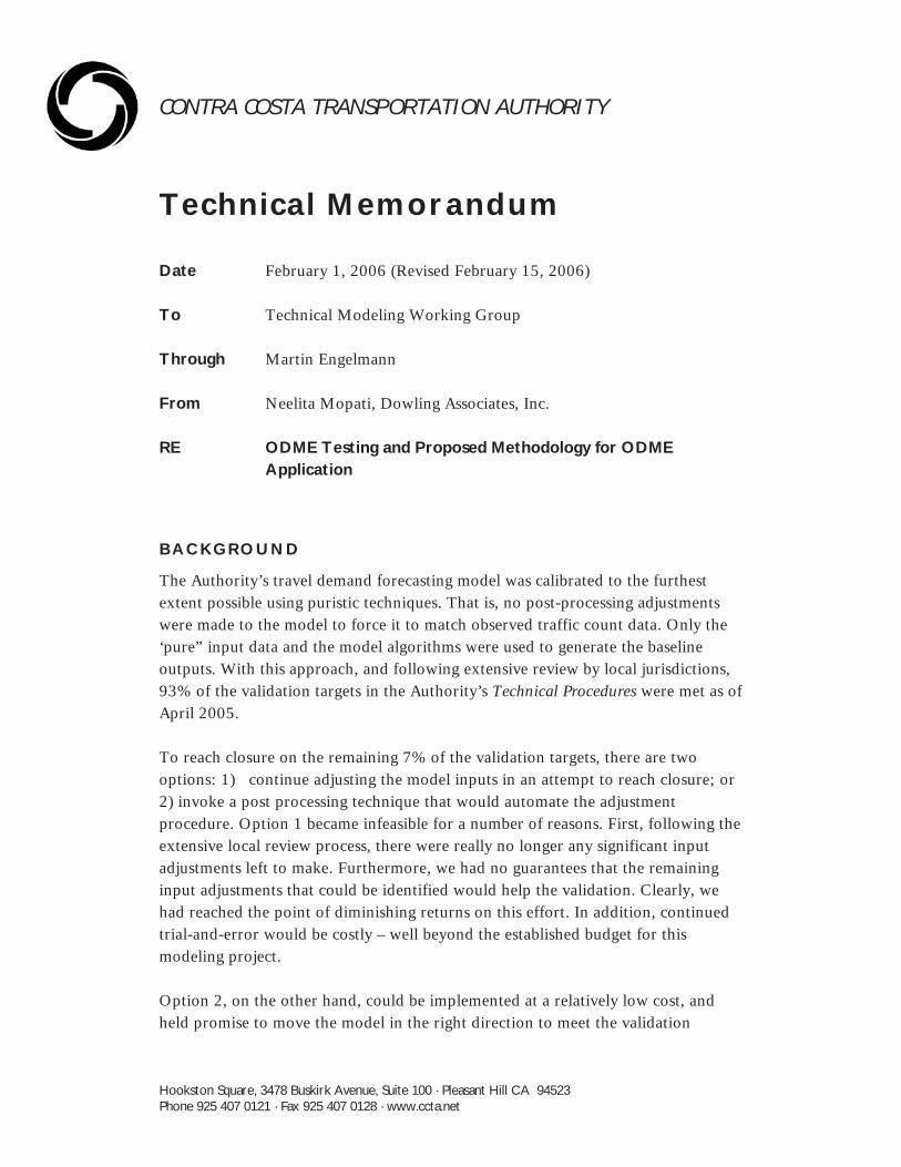
CONTRA COSTA TRANSPORTATION AUTHORITY
Hookston Square, 3478 Buskirk Avenue, Suite 100 · Pleasant Hill CA 94523 Phone 925 407 0121 · Fax 925 407 0128 · www.ccta.net
Technical Memorandum
Date February 1, 2006 (Revised February 15, 2006)
To Technical Modeling Working Group
Through Martin Engelmann
From Neelita Mopati, Dowling Associates, Inc.
RE ODME Testing and Proposed Methodology for ODME Application
BACKGROUND
The Authority’s travel demand forecasting model was calibrated to the furthest extent possible using puristic techniques. That is, no post-processing adjustments were made to the model to force it to match observed traffic count data. Only the ‘pure” input data and the model algorithms were used to generate the baseline outputs. With this approach, and following extensive review by local jurisdictions, 93% of the validation targets in the Authority’s Technical Procedures were met as of April 2005.
To reach closure on the remaining 7% of the validation targets, there are two options: 1) continue adjusting the model inputs in an attempt to reach closure; or 2) invoke a post processing technique that would automate the adjustment procedure. Option 1 became infeasible for a number of reasons. First, following the extensive local review process, there were really no longer any significant input adjustments left to make. Furthermore, we had no guarantees that the remaining input adjustments that could be identified would help the validation. Clearly, we had reached the point of diminishing returns on this effort. In addition, continued trial-and-error would be costly – well beyond the established budget for this modeling project.
Option 2, on the other hand, could be implemented at a relatively low cost, and held promise to move the model in the right direction to meet the validation

Technical Modeling Working Group Wednesday, August 09, 2006 Page 2
targets. Consequently, an automated technique called ODME was developed and applied to meet the remaining 7% of the validation targets.
This discussion paper presents test results of the ODME process and a proposed policy for implementation of ODME in practice
Initial testing of the ODME procedure began in TransCAD version 4.6. The procedure in that version, however, was found to adjust all OD pairs, irrespective of whether a particular OD pair was subject to ODME adjustment. In August 2005, Caliper Corporation technical support was notified of this error, and Caliper proceeded to correct it for the next release of TransCAD. Consequently, the 4.8 version of TransCAD – released in December 2005 – had a corrected ODME procedure. All of the tests shown below were performed using a beta-test version of TransCAD 4.8 that became available in October 2005. The tests were subsequently confirmed on the “official” 4.8 release version, and found to be the same as with the beta-test version.
DESCRIPTION OF THE ODME PROCEDURE
The TMWG first discussed the ODME procedure at its April 2005 meeting. At that time, a memo that broadly explained the technique was distributed and is included in Exhibit 1. Following that discussion, much work was conducted to develop and implement an ODME procedure for review by the TMWG in late 2005. Below is a description of the procedure and results as reviewed by TMWG on December 14, 2005.
The technical process, as it occurs in TransCAD 4.8, is illustrated in the flow chart shown in Figures 1 and 2. The approach TransCAD uses is somewhat different than the early approach used with the previous EMME/2 models (see Exhibit 2).
There are two types of matrix estimation methods that are available in TransCAD 4.8 - Single Path and Multiple Path. In the Single Path method, after the assignment, for each O-D pair, the counts along the best single path are compared with the counts and updated accordingly. In the Multiple Path method, for each O-D pair, the counts along a number of best paths are compared and updated. The Multiple Path method is an improvement over the Single Path method, and can yield more accurate results.

Technical Modeling Working Group Wednesday, August 09, 2006 Page 3
In the Multiple Path method, a number of different best paths need to be determined for each O-D pair. This requires a second assignment to be performed within each O-D update iteration. The first assignment is done to calculate the volume. The second assignment is done to calculate the paths. The number of iterations for the first assignment is controlled in the Globals section of the ODME dialog box. The number of iterations used for the second assignment is referred to as the "Inner Iterations" under the O-D Matrix Estimations Settings. The "Outer Iterations" refers to each O-D matrix update. A flow chart of this process is shown in Figure 1. Figure 2 provides the equations governing the origin-destination matrix adjustments.
Because the Multiple Path method is more accurate than the Single Path method, we used the Multiple Path method in all ODME testing described here.
Since ODME can adjust to any given set of counts, we also have explored application of ODME as a method for establishing an interim base-year validation run (say 2007) based upon ground counts available within a study area for that specific time period.
ADJUSTMENT PARAMETERS
Several adjustment parameters are available to the user in the 4.8 ODME procedures:
Normalization: After ODME, the trip table can be adjusted so that the total Origins and Destinations match the original trip table. The adjustment in TransCAD 4.8 restores changes to the specific OD pairs so that total trips of adjusted OD pairs match the original trip table. This process, however, has the unintended consequence of reversing the benefits of the ODME adjustments. An improvisation on this normalization routine would be to be able to keep the zonal level in and out trips the same while modifying only the trip distributions.
Factor Limits: The user may specify limits to the adjustments factors that ODME will apply to the OD matrix. For example, a maximum factor of 0.75 to 1.5 could be established as the limits on changes to any origin or destination cell. After ODME, the change in trips for each cell is calculated and adjusted back to reflect a maximum change in trips by the factor specified. By applying factor limits, the model user may contain the potential loss of integrity that the trip table could otherwise suffer if the factors are left unbounded.
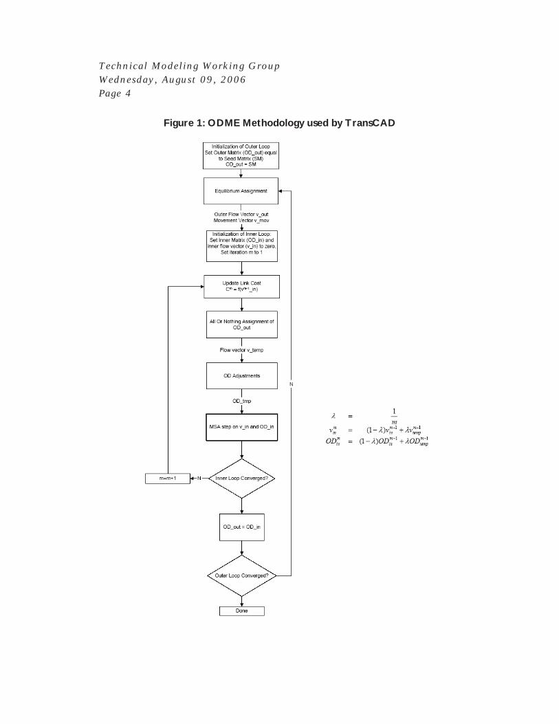
Technical Modeling Working Group Wednesday, August 09, 2006 Page 4
Figure 1: ODME Methodology used by TransCAD

Technical Modeling Working Group Wednesday, August 09, 2006 Page 5
Figure 2: Origin-Destination adjustment logic for each OD pair
Weighting: A further useful parameter is weighting. All counts/targets can be weighted to establish a structure for prioritizing one targets over another in order of importance. For example, weighting may be used to set gateway/cordon line constraints as a high priority target, with adjacent screenline targets set at a lower priority. The gateway constraint becomes, in effect, a non-negotiable target, while the screenlines will receive some, but not all of the ODME adjustments.
Subarea ODME: This option allows the user to specify a subarea (selection of zones) around the study area and run the ODME only on the subarea. This permits the user to control the OD pairs to adjust and also be consistent with the adopted

Technical Modeling Working Group Wednesday, August 09, 2006 Page 6
model. Further control of the subarea cordon volumes is possible by the use of weighting.
PILOT TESTING OF THE ODME PROCESS
To demonstrate the affects of ODME, DA ran several pilot tests in 4.8. Beginning with the first example, which shows the results of one target, we progress to using one screenline, to several screenlines, and finally, to application of all available screenlines.
Initial runs of the full 2,700-zone Countywide Model took more than 24 hours to run for one time period. For the purposes of testing the ODME model, the West County subarea was segmented from the model and used to analyze ODME. Using just the West County portion of the model for assignment purposes, this 308 zone model took only 1.5 hours to run. Following the subarea tests, the full model was used to perform tests using all screenlines.
Single Target Test
As an initial test for ODME, a single target test was conducted on the Bay Bridge using I-80 Westbound in the a.m. peak. The Authority’s Countywide Model is designed to allow this link to be over assigned in the 2000 validation run to compensate from upstream queuing at the Bay Bridge Toll Plaza. The single target test set this volume at the actual count of 10,000, while the initial assignment for 2000 is 15,229. A weighting of 1000 was selected.
Results:
� Impact on Target Area: The final assigned volume on the Westbound Bay Bridge after applying ODME was 9,773 in the AM Peak Hour;
� Impact on surrounding area: A difference plot of traffic assignment with and without ODME for the Bay Bridge is shown in Figure 3. ODME does not conserve trips; hence in order to match the lower Bay Bridge count, all the trips using the Bay Bridge are decreased.

Technical Modeling Working Group Wednesday, August 09, 2006 Page 7
Figure 3: Difference in traffic due to ODME on the Bay Bridge
� Changes to the OD matrix: The range of change by total origin and destination trips of all affected OD pairs is as follows:
Percent Change OriginsZones
DestinationZones % Origins
%Destinations
No Change 259 300 10% 12% Below 10% 1487 1249 58% 50% 10-25% 616 708 24% 28% 25-50% 100 122 4% 5% 50-100% 72 104 3% 4% 100-200% 13 15 1% 1%

Technical Modeling Working Group Wednesday, August 09, 2006 Page 8
Change in Trips (by zone pair) after ODME
0%5%
10%15%20%25%30%35%40%
-150 -100 -50 0 50 100 150 200
Percentage Change in trips
% o
f Zon
e Pa
irs
chan
Percent Change OriginsZones
DestinationZones % Origins
%Destinations
Above 200% 14 21 1% 1%
� Change by zone pair: A histogram of the change in AM Peak Hour trips by percent of zone pair in each range is shown in the chart below. About 40% of the trips do not change and 15% of the cells decrease by 100%.
� Changes in County to County Trips: The difference in County to County trips due to trip adjustments of the Bay Bridge ODME is summarized below. It is interesting to note that the even trips between counties that should not be affected by the Bay Bridge ODME like San Mateo to Santa Clara, which are slightly affected by 4%. Also Sonoma to Napa – OD pairs that presumably would not use the bridge – decreases 19%. On the other hand, trips from Alameda to Contra Costa do not change at all. One reason for this might be the adjustments made to OD trips not passing through target counts as shown in Equation 1 of the ODME methodology in Figure 2.
Destination County Origin County San Francisco San Mateo Santa Clara Alameda Contra Costa Solano Napa Sonoma Marin TOTAL San Francisco 14% -5% -21% -8% -22% -21% -20% -25% -19% 6% San Mateo -10% 8% -4% -9% -24% -19% -20% -23% -11% 3% Santa Clara -20% 5% 4% 1% -9% -5% 9% 11% 15% 4% Alameda -50% -18% -19% 8% 0% -23% -15% -10% -6% 2% Contra Costa -54% -31% -24% -3% 0% -1% -10% 10% 0% -3% Solano -40% -45% -14% -5% -4% 18% 22% 15% 15% 11% Napa -45% -37% -10% -27% -18% 4% 11% 3% -3% 8%

Technical Modeling Working Group Wednesday, August 09, 2006 Page 9
Destination County Origin County San Francisco San Mateo Santa Clara Alameda Contra Costa Solano Napa Sonoma Marin TOTAL Sonoma -48% -51% -17% -36% -27% -20% -19% 10% -14% 5% Marin -24% -29% -27% -17% -20% -13% -13% 15% 9% 1% TOTAL BAY AREA -6% 3% 2% 2% -1% 12% 8% 10% 4% 3%
Single Screenline Tests
I-15: Richmond San Pablo: The only screenline not within 15% of validation counts is I-15 in the PM Peak Hour. So, this screenline was selected for testing the ODME process for a single screenline. Further, to reduce the time taken to run ODME, a subarea of all West County zones was created and the ODME process was tested on the subarea. Figure 4 shows the screenlines in West County. Screenline I-15 runs north to south, parallel and to the west of I-80.
The following ODME scenarios were tested for Screenline I-15 on the West County Subarea:
1) Use only the I-15 counts as targets2) Use the I-15 counts as targets, plus use the model volumes as subarea
externals (from the complete model) with heavy weighting. This enables a user to modify a subarea and still be consistent with the model outside the subarea.
3) ODME on I-15 using actual counts (R1 and Cordon) as subarea externals with heavy weighting.
4) ODME on I-15 using actual counts (R1 and cordon ) as subarea externals with heavy weighting and a maximum factoring or 10%
5) ODME on I-15 using actual counts (R1 and cordon ) as subarea externals with heavy weighting and a maximum factoring or 50%
6) ODME on I-15 using actual counts (R1 and cordon ) as subarea externals with heavy weighting and a maximum factoring or 100%
7) ODME on I-15 using actual counts (R1 and cordon ) as subarea externals with heavy weighting and a maximum factoring or 200%

Technical Modeling Working Group Wednesday, August 09, 2006 Page 10
Figure 4: Internal and Regional Screenlines in West County
Results:
� Impact on target area and surrounding area: A comparison of ODME I-15 is shown in the table below:

Technical Modeling Working Group Wednesday, August 09, 2006 Page 11
No. Name2000 PM Count
I-15 2000 Validation
I-15 ODME No
Externals
I-15 ODME with External
Model Volumes
I-15 ODME with External
Counts
I-15 ODME with External Counts
(Max Change 10%)
I-15 ODME with External Counts (Max Change 50%)
I-15 ODME with External Counts
(Max Change 100%)
I-15 ODME with External Counts
(Max Change 200%)
I14 Richmond 21,520 4% -12% 1% -1% -16% -12% -7% -1%I15 Rich/Sanpb 13,039 -16% 5% 0% -1% -30% -18% -13% -1%I18 Pinole/County 21,193 9% -4% 8% 0% -11% -7% -3% 0%Cordon LCordon Line 23,446 -3% -22% -5% 0% -20% -15% -9% 0%R1 West/Central 6,090 -2% -17% -4% -1% -19% -11% -9% -1%R8 S.C West 17,711 1% -16% -4% -13% -19% -16% -13% -13%
Screenline
All Screenlines in West County
The ODME process was tested for all counts in West County using R1 and Cordon counts in West County with heavy weighting.
Results:
� Impact on targets : A comparison of ODME results for all west county screenlines is shown in the table below.
Screenline
No. Name 2000 PM Count 2000 Validation % Diff
ODME All West County Screenlines
I14 Richmond 21,520 4% 1% I15 Rich/Sanpb 13,039 -16% -2% I18 Pinole/County 21,193 9% -5% CordonLine Cordon Line 23,446 -3% -1% R1 West/Central 6,090 -2% -7% R8 S.C West 17,711 1% -5%
� Change by zone pair: A histogram of the change in AM Peak Hour trips by percent of zone pair in each range is shown in the chart below. About 25% of the cells do not change at all and 22% of the OD trips are reduced to zero.

Technical Modeling Working Group Wednesday, August 09, 2006 Page 12
Change in Trips (by zone pair) after applying ODME in AM Peak Hour
0%
5%
10%15%
20%
25%
30%
-150 -100 -50 0 50 100 150 200
Percentage Change in trips
% o
f Zon
e Pa
irs c
han
All Screenlines in Contra Costa County
Following tests for the subarea level, the full model was run using all screenline counts as targets in the AM Peak Hour, with no factoring and no normalization.
Results:
� Impact on targets: The ODME process produced good results for all the screenlines in the AM peak hour. The screenline comparison report is shown in below.
Internal Screenlines
Screenline AM PEAK HOUR
No. Name 2000 AM Count
2000 AM ODME
2000 AM Model
ODME % Diff
Validation % Diff
I1 SR 4 23,967 23,490 26112 -2% 9%
I2 Concord 29,027 28,551 30312 -2% 4%
I3 Orinda 16,523 15,668 17171 -5% 4%
I4 I-680 39,372 40,021 36460 2% -7%
I5 Treat 34,701 33,828 36244 -3% 4%
I6 Ygnacio 29,072 28,142 29641 -3% 2%
I7 SR24 5,356 5,141 4873 -4% -9%
I8 Walnut Creek 27,465 27,083 30318 -1% 10%
I9 San Ramon 14,779 14,261 14907 -4% 1%

Technical Modeling Working Group Wednesday, August 09, 2006 Page 13
Screenline AM PEAK HOUR
No. Name 2000 AM Count
2000 AM ODME
2000 AM Model
ODME % Diff
Validation % Diff
I10 Danville(NB / SB) 7,002 6,790 7118 -3% 2%
I11 Danville (EB / WB) 7,564 7,438 6955 -2% -8%
I12 Antioch/Brentwood 6,727 6,699 6555 0% -3%
I13 Oakley/Brentwood 6,412 6,443 6951 0% 8%
I14 Richmond 21,176 21,268 21785 0% 3%
I15 Rich/Sanpb 16,118 16,232 14890 1% -8%
I16 I-580 23,939 23,262 22394 -3% -6%
I17 West Livermore 20,486 19,962 20713 -3% 1%
I18 Pinole/County 20,701 19,296 22568 -7% 9%
18 of the 18 Screenlines meet target 18 of 18 Meet TargetTOTAL – Internal
350,387 343,575 355967 -2% 2%
Regional Screenlines
Screenline AM PEAK HOUR
No. Name 2000 AM Count
2000 AM ODME
2000 AM Model
ODME % Diff
Validation % Diff
CordonLine Cordon Line 86,122 83,057 82390 -4% -4%
R1 West/Central 5,743 5,734 6166 0% 7%
R2 Lamorinda 21,069 19,132 19652 -9% -7%
R3 TriValley 16,823 15,984 19670 -5% 17%
R4 Central/East 16,872 15,866 18483 -6% 10%
R5 S.C Central 6,627 6,374 7171 -4% 8%
R6 S.C East 12,553 12,442 14246 -1% 13%
R7 S.C Tri Valley 14,486 13,705 14671 -5% 1%
R8 S.C West 16,359 15,201 18005 -7% 10%
R9 Alameda County 21,661 21,657 21617 0% 0%
R10 Sunol 9,450 9,506 10243 1% 8%
R11 Greenville 10,641 10,574 10809 -1% 2%
TOTAL – Regional 12 of the 12 Screenlines meet target
10 of 12 Meet Target

Technical Modeling Working Group Wednesday, August 09, 2006 Page 14
Screenline AM PEAK HOUR
No. Name 2000 AM Count
2000 AM ODME
2000 AM Model
ODME % Diff
Validation % Diff
238,406 229,232 243123 -4% 2%
GRAND TOTAL 588,793 572,807 599090 -3% 2%
All Available Counts
Following tests for just the screenline counts, the full model was run using all available screenline and intersection counts as targets, with no factoring and no normalization. Since the main concern was to hit all screenline targets using ODME, screenline counts were weighted higher than intersection counts.
Results:
� Impact on targets: The ODME process produced very good link level validation results for all screenline and intersection counts. The screenline report and the validation are shown below.

Technical Modeling Working Group Wednesday, August 09, 2006 Page 15
No. Name2000 AM Count
2000 AM ODME
2000 AM Model
ODME % Diff
Validation % Diff
2000 PM Count
2000 PM ODME
2000 PM Model
ODME % Diff
Validation % Diff
I1 SR 4 23,967 26,330 26112 10% 9% 25,623 28,274 27876 10% 9%I2 Concord 29,027 29,440 30312 1% 4% 31,414 31,990 31692 2% 1%I3 Orinda 16,523 18,023 17171 9% 4% 15,887 16,667 17229 5% 8%I4 I-680 39,372 41,863 36460 6% -7% 43,621 41,648 39581 -5% -9%I5 Treat 34,701 36,009 36244 4% 4% 36,840 37,527 38556 2% 5%I6 Ygnacio 29,072 28,491 29641 -2% 2% 30,089 30,640 31594 2% 5%I7 SR24 5,356 5,508 4873 3% -9% 5,717 5,428 5709 -5% 0%I8 Walnut Creek 27,465 28,568 30318 4% 10% 29,867 32,953 33122 10% 11%I9 San Ramon 14,779 14,232 14907 -4% 1% 15,943 15,888 16317 0% 2%I10 Danville(NB / SB) 7,002 7,535 7118 8% 2% 7,241 7,678 7006 6% -3%I11 Danville (EB / WB) 7,564 7,928 6955 5% -8% 7,667 7,892 8039 3% 5%I12 Antioch/Brentwood 6,727 7,301 6555 9% -3% 7,918 8,173 7877 3% -1%I13 Oakley/Brentwood 6,412 6,888 6951 7% 8% 7,539 7,932 7858 5% 4%I14 Richmond 21,176 23,335 21785 10% 3% 21,520 23,762 22378 10% 4%I15 Rich/Sanpb 16,118 15,968 14890 -1% -8% 18,589 19,228 15672 3% -16%I16 I-580 23,939 25,721 22394 7% -6% 26,507 25,420 24304 -4% -8%I17 West Livermore 20,486 18,877 20713 -8% 1% 21,015 20,258 22956 -4% 9%I18 Pinole/County 20,701 22,100 22568 7% 9% 21,193 23,084 23067 9% 9%
18 of 18 Meet Target
16 of 18 Meet Target
350,387 364,117 355967 4% 2% 374,190 384,442 380833 3% 2%
No. Name2000 AM Count
2000 AM ODME
2000 AM Model
ODME % Diff
Validation % Diff
2000 PM Count
2000 PM ODME
2000 PM Model
ODME % Diff
Validation % Diff
Cordon Cordon Line 86,122 82,801 82390 -4% -4% 90,766 87,980 88141 -3% -3%R1 West/Central 5,743 5,668 6166 -1% 7% 6,090 5,618 5969 -8% -2%R2 Lamorinda 21,069 19,789 19652 -6% -7% 20,174 20,419 21372 1% 6%R3 TriValley 16,823 16,149 19670 -4% 17% 17,989 16,669 19386 -7% 8%R4 Central/East 16,872 16,208 18483 -4% 10% 17,268 16,921 18579 -2% 8%R5 S.C Central 6,627 7,243 7171 9% 8% 7,408 7,688 8136 4% 10%R6 S.C East 12,553 13,952 14246 11% 13% 14,355 14,817 15846 3% 10%R7 S.C Tri Valley 14,486 13,134 14671 -9% 1% 15,147 13,947 15535 -8% 3%R8 S.C West 16,359 17,238 18005 5% 10% 17,711 17,706 17967 0% 1%R9 Alameda County 21,661 20,105 21617 -7% 0% 18,731 18,005 18553 -4% -1%R10 Sunol 9,450 9,570 10243 1% 8% 11,894 11,634 12917 -2% 9%R11 Greenville 10,641 11,300 10809 6% 2% 11,587 12,033 11959 4% 3%
10 of 12 Meet Target
12 of 12 Meet Target
238,406 233,157 243123 -2% 2% 249,120 243,437 254360 -2% 2%
588,793 597,274 599090 1% 2% 623,310 627,879 635193 1% 2%
18 of the 18 Screenlines meet target 18 of the 18 Screenlines meet target
PM PEAK HOUR
PM PEAK HOUR
AM PEAK HOUR
AM PEAK HOUR
Internal Screenlines
GRAND TOTAL (Regional + Internal)
Screenline
ScreenlineRegional Screenlines
11 of the 12 Screenlines meet target, 1 is +/-15% 12 of the 12 Screenlines meet targetTOTAL - Regional
TOTAL - Internal
Comparison of Screenline Report with and without ODME

Technical Modeling Working Group Wednesday, August 09, 2006 Page 16
Link Based Validation Report with and without ODME
Facility Type and Criteria Number of Counts
LinksMeetingTarget
% of links within target with ODME
% of links within target (validation)
Validation Target
AM PEAK HOUR Freeway Links within 20% 75 72 96% 95% 75% Freeway Links within 10% 75 70 93% 75% 50% Arterials with 10,000+ ADT within 30% 86 81 94% 67% 75% Arterials with 10,000+ ADT within 15% 86 67 78% 37% 50% Intersections with 1000+ Vehicles per hr within 20% 609 514 84% 87% 50% Intersections with 500-1000 Vehicles per hr within 20% 197 157 80% 82% 30% All Intersections within 30% of Counts 893 807 90% 89% 75% All Intersections within 15% of Counts 893 639 72% 76% 50% 80% of Freeway Counts below the Curve 61 48 79% 89% 80% 80% of Ramp Counts below the Curve 450 422 94% 78% 80% Freeways and ramps 511 470 92% 79% 80% PM PEAK HOUR Freeway Links within 20% 75 73 97% 81% 75% Freeway Links within 10% 75 67 89% 68% 50% Arterials with 10,000+ vehicles within 30% 86 84 98% 74% 75% Arterials with 10,000+ vehicles within 15% 86 68 79% 44% 50% Intersections with 1000+ Vehicles per hr within 20% 663 551 83% 86% 50% Intersections with 500-1000 Vehicles per hr within 20% 164 125 76% 71% 30% All Intersections within 30% of Counts 907 793 87% 53% 75% All Intersections within 15% of Counts 907 617 68% 29% 50% 80% of Freeway Counts below the Curve 61 53 87% 82% 80% 80% of Ramp Counts below the Curve 450 412 92% 77% 80% Freeways and ramps 511 465 91% 78% 80%
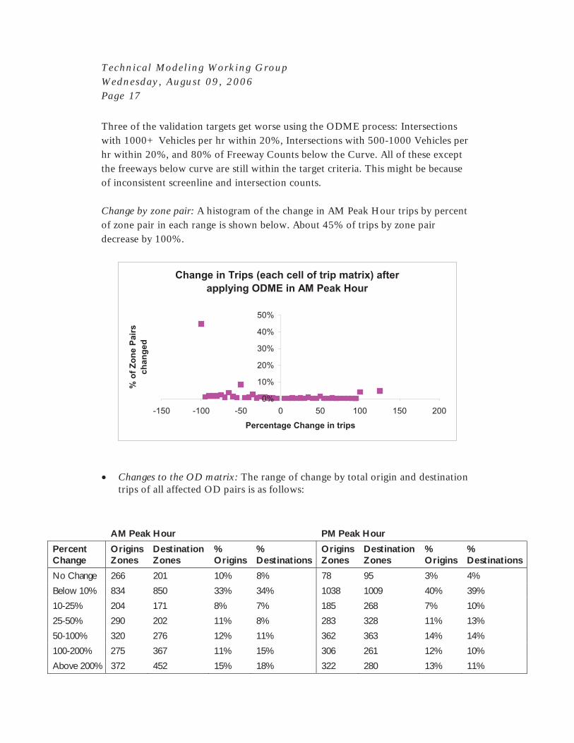
Technical Modeling Working Group Wednesday, August 09, 2006 Page 17
Three of the validation targets get worse using the ODME process: Intersections with 1000+ Vehicles per hr within 20%, Intersections with 500-1000 Vehicles per hr within 20%, and 80% of Freeway Counts below the Curve. All of these except the freeways below curve are still within the target criteria. This might be because of inconsistent screenline and intersection counts.
Change by zone pair: A histogram of the change in AM Peak Hour trips by percent of zone pair in each range is shown below. About 45% of trips by zone pair decrease by 100%.
� Changes to the OD matrix: The range of change by total origin and destination trips of all affected OD pairs is as follows:
AM Peak Hour PM Peak Hour Percent Change
OriginsZones
DestinationZones
%Origins
%Destinations
OriginsZones
DestinationZones
%Origins
%Destinations
No Change 266 201 10% 8% 78 95 3% 4% Below 10% 834 850 33% 34% 1038 1009 40% 39% 10-25% 204 171 8% 7% 185 268 7% 10% 25-50% 290 202 11% 8% 283 328 11% 13% 50-100% 320 276 12% 11% 362 363 14% 14% 100-200% 275 367 11% 15% 306 261 12% 10% Above 200% 372 452 15% 18% 322 280 13% 11%
Change in Trips (each cell of trip matrix) after applying ODME in AM Peak Hour
0%
10%
20%
30%
40%
50%
-150 -100 -50 0 50 100 150 200
Percentage Change in trips
% o
f Zon
e Pa
irs
chan
ged

Technical Modeling Working Group Wednesday, August 09, 2006 Page 18
Trip Length Distribution
0.00
10.00
20.00
30.00
40.00
50.00
60.00
0 10 20 30 40 50 60
Trip Length (Miles)
% D
rive
Alo
ne T
rips
Pre ODME Drive AloneDistributionPost ODME Drive AloneDistribution
Trip Length Distribution
0.00
10.00
20.00
30.00
40.00
50.00
60.00
70.00
0 10 20 30 40 50 60
Trip Length (Miles)
% S
hare
d R
ide
3+ T
rips
Pre ODME Shared Ride 3+DistributionPost ODME Shared Ride 3+Distribution
� Changes to the trip length distribution: At the December 14, 2005 TMWG meeting, a concern was raised regarding the impact of ODME on the trip length distribution. In response to this concern, DA developed the figures below to determine whether the trip-length distribution by mode was adversely affected by the ODME procedure. Shown below is a comparison of the pre- and post-ODME trip distribution for the ODME run with all available counts by Drive Alone and Shared Ride 3+ modes. The Matrix Estimation process seems to create more short length trips for both the Drive Alone and Shared Ride classes when compared to the distribution before adjustment. The effect is greater for the drive alone trips since they make up about 85% of all trips. This suggests that adjustments are made to closer O-D pairs contributing to a count rather than farther O-D pairs. However, the overall affect appears insignificant.

Technical Modeling Working Group Wednesday, August 09, 2006 Page 19
SUMMARY OF RESULTS
Overall, the ODME process in TransCAD 4.8 was able to match target counts very well. The pilot testing produced consistent results for all test cases. The ODME test using all screenline and intersection counts proves that it is a useful tool that can help reach closure on the remaining 7% of the validation targets as well as produce good link level validation results.
Some of the ODME adjustment parameters like normalization and factoring available in TransCAD 4.8 neither help in matching target counts nor maintain trip table consistency. In fact, these parameters as currently applied serve to reverse the benefits of the ODME adjustments. While both of these parameters serve as useful tools for other applications of TransCAD, they did not help toward achieving the specific ODME objectives we are pursuing here. To add utility for the CCTA application, both adjustment parameters would need to be applied during the matrix estimation process instead of after it. For example, if a maximum change factor of 50% is applied within ODME, the adjustment process will try to hit counts while making sure that no cell in the trip table goes over 1.5 times its value. The same factor, when applied after completion of the ODME procedure, restores all ODME-adjusted pairs to the 1.5 factor limit, without re-checking the assignment against the target value. As seen in the test cases for screenline I-15 in Richmond, the benefits attributable to ODME are reversed through this technique, consequently, use of factoring is not recommended. Similarly, normalization is not recommended for implementation in the CCTA method.
Use of the subarea windowing feature in TransCAD coupled with the ODME process proves to be a useful way to reduce run time for local validation applications, while maintaining consistency with the regional model. The dramatic decrease in the ODME run-time will be especially useful when numerous trial-and-error runs are required.
Weighting is another valuable parameter than can be used to prioritize target counts for ODME. Subarea ODME for West County using high weights for the cordon lines and lower weights for I-15 was within target not only for I-15 but also for other screenlines in West County, showing that the matrix adjustments were moving in the right direction.
Changes to the demand trip table during the ODME process are of particular concern. With a high number of target counts as the test case using all screenline and intersection counts, about 50% of the OD pair trips are zeroed out during
Technical Modeling Working Group Wednesday, August 09, 2006 Page 20
ODME. On the other hand, with a single target like the Bay Bridge, 40% of the cells are unchanged while 15% are zeroed out. However, at the zonal level, the in and out trips for a zone change by only 10% for more than half the zones. On the county level, depending on how regional the target count is, county-to-county trips may be affected as well, and should be monitored accordingly.
A further area of concern is the effect of ODME on the integrity of the trip-length distribution table. Based upon the above analysis, it appears that changes to the trip-length distribution are minimal. This suggests that ODME can be successfully implemented without disturbing the trip-length results, provided the model user implements ODME under conditions similar to those tested above, and consistent with established guidelines.
ODME IMPLEMENTATION GUIDELINES
Based upon the above investigation, the following guidelines are proposed for incorporation into the Authority’s Technical Procedures, subject to review and approval by the TMWG and TCC:
� Use of ODME is an optional validation tool that may be invoked only after calibration and validation efforts have been conducted to the fullest extent feasible. [We propose, as a guideline that90% of the screenlines should be within targets before the ODME tool is utilized.] ODME should not be used to compensate for network and land use inaccuracies that cause poor traffic assignments. Rather, ODME is to be applied only as a refinement after all inputs to the model have been fully reviewed and can no longer be adjusted without deviating from the empirical inputs.
� The ODME process can provide a better match to traffic counts, but is not behaviorally-based and so is not recommended for implementation at a county-wide level. It can, however, be effectively applied at the subarea and local levelto provide a better fit with observed data. In tests performed on regional county-wide targets, it was observed that the benefits of ODME diminished as the number of targets increased. When the ODME procedure encounters large number of conflicting count data, the validation results tend to degrade, because the ODME process compromises the trip table to meet all of the input targets.
� The successful application of ODME at the subarea level also suggests that the procedure could be applied successfully to re-calibrate the model to a post-2000

Technical Modeling Working Group Wednesday, August 09, 2006 Page 21
interim horizon year for which traffic counts are available within a particular study area.
� “Windowing” can be used to apply ODME to local areas. Subarea ODME helps in maintaining consistency with the regional model while improving local validation. This also reduces the run time dramatically because of a much smaller analysis data set. Because of consistency issues with the regional model, however, use of windowing was not supported by the TMWG.
� The number of count targets input by the model user is flexible. However, based on ODME tests conducted, a single target count,is not recommended For gateway constraint applications, a single directional peak hour link volume target should be accompanied by counts/model volume constraints at key strategic locations to preserve model validity. Weighting can be used to prioritize specific count targets over others. Use of selected targets, for example, one or multiple screenline targets can help address a specific validation issue within a specific study area. Alternatively, all available count data within a subarea can be input to improve overall validation. However, inconsistencies in the count data may interfere with achieving convergence. Conflicting count data may be the result of congestion, queuing, or variations in the time of day and/or the season during which adjacent counts were collected. Consequently, juxtaposing conflicting targets will result in fewer of the validation criteria being met, because the ODME matrix balancing process will be unable to achieve convergence for all targets.
� Applying ODME on a congested network might artificially lower the volumes to the constrained counts. Therefore, instead of using congested counts, which are generally low, it is recommended to set the target volume at maximum capacity on freeway locations experiencing recurrent congestion.
� In the absence of counts by mode, the ODME process setup for the CCTA Model applies matrix adjustments on the combined trip table and uses the original zonal level mode splits on the estimated trip table. If counts are available to the user by mode, it is advisable to use the ‘Multi-Class ODME” process available in TransCAD to better assign multi-modal volumes on the network.
� To preserve the model’s integrity, and to maintain consistency with the regional model, the model user should carefully evaluate the effect of ODME on the adjusted O/D trip table before applying the assignment results. O/D pairs that do not cross an ODME target screenline or count location should not be significantly affected by the ODME adjustment process. In addition, trip length distributions should be compared before and after ODME to ensure that traffic distribution patterns have not been compromised.

Technical Modeling Working Group Wednesday, August 09, 2006 Page 22
� The TransCAD interface will allow the model user to specify the number of iterations and the desired percentage convergence tolerance for the ODME procedure. This will determine running time for the ODME operation. [Basedon tests and discussions with Caliper Corporation, the recommended inner loop iterations are 50 and outer loop iterations are 20. A convergence percentage tolerance of 5% is sufficient.]
� Adjustments to the future trip table should be made after ODME is successfully applied to the base year following the above guidelines. The difference between the original multi-modal trip table and the estimated trip table by mode shall be added to the unadjusted future trip table by mode. The adjusted future trip table should be re-assigned using Multi-Class Assignment in TransCAD to obtain the forecast volumes.
PROCEDURE FOR APPLYING ODME
The following procedures will be included in the Model User’s Guide as directions to run ODME:
� Run the “puristic” model validation for the base year (year 2000) from Initialization to Assignment. Any changes to the land use or model network should be made prior to running the model. Changes made after running the model and before running ODME will be ignored.
� Generate screenline report and validation report. Instructions to generate screenline reports are included in the User’s Guide. Reproduce and check the results of the validation run against the Authority’s model documentation. In case of changes to the model or local revalidation, 90% of the screenlines should be within targets.
� Input count targets and “weights” for counts by time period in a separate database by network link ID. A sample count table used for ODME is provided as part of the model files. If the user has count information by mode, then additional columns should be added to the database to include these counts.
� Using the user-interface, select and run the ODME process on the entire network or a subarea. If running ODME on a subarea, the “Create Subarea for ODME” process as shown below should be run earlier to the ODME step.

Technical Modeling Working Group Wednesday, August 09, 2006 Page 23
� Compute trip table differences before and after ODME. Create 9 county summaries if using the entire network. Compare tables and check for reasonableness.
� Check assignment differences for rationality of results and validation to count targets;
� Apply differences to forecast by running the same ODME step for the future year. The ODME difference trip table should be copied into the future year model run folder. In the absence of such a file, the process will provide the message below and hang. If running the Subarea ODME, a Subarea needs to be created for the forecast year before transferring trip table changes.
� Check forecast ODME assignment for reasonableness.
USING ODME TO ESTABLISH AN INTERIM BASELINE HORIZON YEAR
The Authority’s model is validated to year 2000 traffic counts. The next decennial model update will involve a re-validation to 2010 traffic data. In the interim, model users may wish to use the model to test existing conditions, and forecast results, based upon post-2000 interim horizon year (say 2007) for which traffic counts are available within the study area. The ODME procedure could be a useful tool for quickly re-calibrating the year 2000 model run to a post-2000 interim set of counts, provided that overall regional consistency is preserved through a parallel interpolation process for the regionwide land use data set. To take advantage of this option, the following steps are recommended. These should be carried out consistent with the above ODME guidelines as outlined for conventional (Year 2000) applications.:

Technical Modeling Working Group Wednesday, August 09, 2006 Page 24
� The interim year model run should be developed using the fully validated pre-ODME year 2000 model run, and the corresponding 2010 model run.
� An interim-year land use data base should be developed by interpolating between 2000 and 2010. Alternatively, if land use analysis is not required, the vehicle trip tables for these two horizon years may be used as a basis for interpolation to a new base year.
� Run the interim base-year model through assignment to establish the pre-ODME interim assignment for (say) 2007.
� Assign target volumes for the study area, based upon actual counts. � Run ODME on the interim horizon year assignment. � Use the post-ODME results as the new interim-base year validation run. � Apply the differences between pre-and post ODME vehicle trip table for the
interim year to the forecast year.

Technical Modeling Working Group Wednesday, August 09, 2006 Page 25
EXHIBIT 1
Memorandum
TO: Martin Engelmann, CCTA
FROM: Maren Outwater and Vamsee Modugula, CS
DATE: April 12, 2005
RE: Application of Trip Table Estimation Techniques for the Contra Costa Countywide Travel Model
The objective of the calibration of the Contra Costa Countywide Travel Model was to capture travel behavior within Contra Costa County and match observed traffic and transit counts within the county, as well as to provide overall consistency with the MTC regional travel model. The validation standards established at an aggregate and screenline level all serve to achieve this objective. Additional objectives to have the model provide accurate link and turn-level volumes for subarea, corridor or site studies can be met by refining the model in these locations and further by implementing trip table estimation procedures to adjust model outputs to more closely match traffic counts. These trip table estimation procedures can provide a better match to traffic counts, but are not behaviorally-based so are not recommended at a county-wide level. Nonetheless, they can be applied and used for local area studies to provide a better fit with observed data.

Technical Modeling Working Group Wednesday, August 09, 2006 Page 26
There are a variety of trip table estimation techniques that have been tested and used in the transportation planning field over many years. One demonstration of this is discussed in a paper by Alan Horowitz1. Caliper Corporation has incorporated one of these techniques into the TransCAD software package, called Origin-Destination Matrix Estimation (ODME). TransCAD documentation presents a summary of the process, as follows:
The O-D Matrix Estimation procedure in TransCAD is based on the work of Nielsen (1993), who independently developed it as a procedure for TransCAD 2.1. The method was re-implemented by Caliper Corporation. This method has the advantages of treating counts as stochastic variables, as well as working with any traffic assignment method. It therefore is attractive for use with the Stochastic User Equilibrium Assignment method, as well as with User Equilibrium Assignment. Nielsen's method is an iterative (or bi-level) process that switches back and forth between a traffic assignment stage and a matrix estimation stage. The procedure requires an initial estimate of the O-D matrix. This can be a default, be a prior estimate based upon survey measurements, or be synthetically generated (e.g., from a doubly-constrained trip distribution model). The success of this method is based upon use of a realistic traffic assignment model. Otherwise, a biased trip table will be produced. In practice, Nielsen's method appears to work quite well, and many users have reported good results with its use.
The TransCAD model documentation documents the process to implement this trip table estimation procedure in detail, and can be used to refine the model volumes for a corridor, small area, or traffic impact study by local jurisdictions. It was purposely not used to validate the countywide model, given the lack of behavioral realism in the procedure, but this is not considered to be a problem at a local level.
1 Alan Horowitz, Tests of a Family of Trip Table Refinements for Long-Range, Quick-Response Travel Forecasting, Center for Urban Transportation Studies, University of Wisconsin – Milwaukee, http://www.uwm.edu/~horowitz/ODTableRefinement.pdf.

Tec
hnic
al M
odel
ing
Wor
kin
g G
rou
p W
edn
esda
y, A
ugu
st 0
9,
20
06
Pa
ge 2
7
PRO
POSE
D O
DM
E PR
OC
EDU
RE
FOR
CO
NTR
A C
OST
AIN
CO
RPO
RA
TIN
G T
HE
GR
AD
IEN
T AP
PRO
AC
H
STA
RT
RE
AD H
IGH
WAY
FL
OW
S P
KH
RFL
OW
.BIN
RE
AD
TAR
GET
V
OLU
ME
S[F
OR
MU
LA]
IDEN
TIFY
LIN
KS
W
ITH
TA
RG
ET V
OLU
MES
CO
UN
T N
UM
BER
O
F LI
NK
S W
ITH
TA
RG
ET V
OLU
MES
CR
EATE
DIR
EC
TOR
IES
FO
R E
AC
H L
INK
THAT
H
AS
A T
AR
GET
VO
LUM
E
AS
SIG
NE
D T
O IT
EN
ABL
E TR
AN
SFER
OF
AD
JUST
ED
TR
IPTA
BLE
FR
OM
ON
E
SEL
ECT
LIN
K C
YCLE
TO
TH
E N
EXT
A
MP
KHR
FIN
X.M
TX.
(Ste
p (b
) bel
ow)
ASS
IGN
ED
VO
LUM
ES =
[FO
RM
ULA
]
HO
W T
HE
PR
OG
RA
M C
YCLE
S T
HR
OU
GH
MU
LTIP
LE
SE
LEC
T LI
NKS
IS T
O B
E D
ETE
RM
INE
D:
US
E T
HE
MO
ST
EFF
ICIE
NT
AP
PRO
ACH
--EI
THER
1) P
ER
FOR
M O
NE
IT
ER
ATIO
N O
N E
AC
H T
AR
GET
IN S
ERIE
S, O
R 2
) PE
RFO
RM
M
ULT
IPLE
ITER
ATI
ON
S O
N A
SIN
GLE
TAR
GE
T TO
C
ON
VE
RG
EN
CE
.
[FO
RM
ULA
]
A
TAR
GET
VO
LUM
ES
AR
E TH
E O
BSE
RVE
D V
OLU
MES
[FO
RM
ULA
]
EX
HIB
IT 2

Tec
hnic
al M
odel
ing
Wor
kin
g G
rou
p W
edn
esda
y, A
ugu
st 0
9,
20
06
Pa
ge 2
8
PER
FOR
M S
ELEC
T LI
NK
ON
SIN
GLE
LIN
K [F
OR
MU
LA]
SAV
E O
/D P
AIR
S TH
AT
US
E SE
LEC
TED
LIN
KSE
L_LI
NK_
OD
.MTX
CO
MPU
TE “D
ISTA
NC
E”BE
TWEE
N
OB
SE
RVE
D [F
OR
MU
LA]
AN
D A
SS
IGN
ED
VO
LUM
ES F
OR
[FO
RM
ULA
]
CO
MP
UTE
OPT
IMA
L G
RA
DIE
NT
STE
P L
EN
GTH
[FO
RM
ULA
]
CH
EC
K ST
EP
LEN
GTH
(TH
IS W
ILL
EVE
NTU
ALLY
BE B
OU
ND
ED)
OB
JEC
TIVE
: M
INIM
IZE
DIS
TAN
CE
BE
TWE
EN
O
BSER
VED
AN
D A
SSI
GN
ED V
OLU
MES
[ FO
RM
ULA
13]
(1)
BA
PER
CE
NT
TOLE
RA
NC
E M
ET O
R M
AX
NU
MB
ER O
F IT
ER
ATIO
NS
EXC
EED
ED
FOR
ALL
LIN
KS?
[FO
RM
ULA
]
SA
VE
FIN
AL
TRIP
TA
BLE
(AM
PKH
RFI
NZ.
MTX
)AN
D F
INAL
AD
JUST
ED H
IGH
WAY
FLO
WS
(PKH
RA
MFL
OW
869.
BIN
)
RE
POR
T FI
NAL
RES
ULT
S
END
NO
YES
a -z
(a)
[FO
RM
ULA
1 ]
(2)
(16) (13)
[FO
RM
ULA
2 ]
[FO
RM
ULA
16
]
F

Tec
hnic
al M
odel
ing
Wor
kin
g G
rou
p W
edn
esda
y, A
ugu
st 0
9,
20
06
Pa
ge 2
9
RE
AD
VEH
ICH
LE
TRIP
TAB
LEA
MP
KH
RFI
N.M
TX
DIS
TRIB
UTE
[FO
RM
ULA
] AM
ON
GS
ELE
CTE
D O
/D P
AIR
SID
EN
TIFI
ED
IN (a
) ABO
VE
SE
L_LI
NK_
OD
.MTX
CR
EAT
E A
DD
ITIO
NAL
A
TTR
IBU
TE M
ATR
IX
RE
FLE
CTI
NG
CH
AN
GE
S
IN D
EM
AN
DA
DD
_ATT
RIB
UTE
.OD
.MTX
HIG
HW
AY
LOA
DIN
G
SUM
AD
DIT
ION
ALA
TTR
IBU
TE M
ATR
IX W
ITH
B
EH
ICLE
TR
IP T
ABLE
TO
CR
EAT
E N
EW T
RIP
TA
BLE
AM
PK
HR
FIN
X.M
TX
WH
ERE
G =
NU
MB
ER O
F O
D P
AIR
S W
ITH
P
ATH
S T
HA
T TR
AVE
L TH
RO
UG
H A
S
ELE
CTE
D L
INK
[FO
RM
ULA
]
C
B
CC
TA 2
000_
HW
Y.N
ETH
IGH
WA
Y FL
OW
SP
KH
RA
MFL
OW
1.B
IN(1
-1,0
00)
(b)

Tec
hnic
al M
odel
ing
Wor
kin
g G
rou
p W
edn
esda
y, A
ugu
st 0
9,
20
06
Pa
ge 3
0
CO
MPU
TE “D
ISTA
NC
E”B
ETW
EEN
OBS
ER
VED
[F
OR
MU
LA] A
ND
ASS
IGN
ED
[FO
RM
ULA
]V
OLU
ME
S A
T [F
OR
MU
LA]
FC
US
ER
SPE
CIF
IED
TAR
GE
T/A
SS
IGN
ED
PE
RC
ENTA
GE
TO
LER
AN
CE
(SA
Y 1%
) A
ND
MA
XIM
UM
NU
MB
ER
O
F IT
ER
ATI
ON
S(S
AY
50)
SA
VE
NEW
TR
IP T
ABLE
A
ND
CA
RR
Y FO
RW
ARD
TO N
EXT
LIN
K [F
OR
MU
LA]
AM
PK
HR
FIN
X.M
TX
% T
OLE
RA
NC
E M
ET?
MA
XIM
UM
NU
MB
ER
OF
ITE
RA
TIO
NS
EXC
EE
DE
D?
FYE
S
NO

Appendix G - Guidelines for Application of Gateway Capacity Constraint Methodology


Appendix G GATEWAY CAPACITY CONSTRAINT METHODOLOGY
IIntroduction The methodology described in this section is an update of one developed during 1994 for the Authority by a technical working group comprised of both public and private sector transportation professionals. The group was charged with responding to a situation that commonly arises when using peak-hour travel forecasting demand models in high-growth “traffic sheds”. Any of the available travel demand forecasting modeling software packages—TransCAD, CUBE, EMME/3, VISUM—can give projected peak-hour traffic volumes that significantly exceed estimated peak hour capacity on major freeway corridors. This phenomenon occurs even though these models use capacity-constraining algorithms when assigning traffic to a congested roadway network.
Where travel forecasting models predict that peak-hour volumes will exceed capacity, transportation planners have a good indication that congestion may occur at those locations. But it also raises a concern that the model has assigned too many trips to the highway network during the peak hour. In actual operations, a roadway cannot carry more vehicles than its capacity allows. Drivers must choose to wait in upstream queues, change their time of travel, shift modes, or elect not to travel. This section of the Technical Procedures presents a methodology for working with model output where projected volumes exceed capacity, and for constraining the model output in the framework of the travel demand forecasting model.
The Gateway Capacity Constraint Methodology (GCCM) provides a technique for adjusting model output downward where projected peak-hour volumes significantly exceed capacity on major corridors (or “gateways”) serving a study area. Travel forecasting models generally assign peak-hour vehicle trips to the fastest, most direct route between origin and destination. Once those routes have become congested, the model assigns traffic to alternative, less convenient routes. As demand approaches capacity on all possible alternate routes, the model may continue to assign traffic to the congested routes, even when the demand exceeds capacity.
Where peak-hour volume model outputs exceed capacity, the model is predicting unrealistically high traffic levels and is failing to take into account the physical constraints at the study area “gateways”. For example, in the Tri-Valley, the travel model results for future years may show forecasts of 12,000 vehicles per hour entering the Tri-Valley study area on I-580 over the Altamont Pass in the AM peak hour. I-580 is an eight-lane freeway at Altamont Pass (four-lanes each way) with a capacity of roughly 8,000 vehicles per hour in each direction. In this case the model results are 50 percent beyond the corridor's capacity. The model is simulating how trips converge on a congested gateway, then disperse to downstream facilities. It follows that if projected traffic at any point on the network is unrealistically high, then traffic levels assigned to downstream facilities would also be unrealistically high.

This methodology allows the analyst to specify “not to exceed” peak hour flows at gateways where clear future capacity limitations have been identified. To further constrain only specifically identified gateway links of the highway network, it is necessary to trace the path of each trip from the gateway onto downstream facilities, including freeways, ramps, arterials, and collector and local streets to its final destination. Because doing this by hand would be overly time consuming, this methodology is executed within the framework of the TransCAD modeling software.
DDescription of Methodology TransCAD features an ODME (Origin-Destination Matrix Estimation) procedure that allows the user to constrain the peak hour vehicle trip OD table to the capacity of selected road links in the network. The ODME procedure is described in Section 8 of these procedures and in the Model Users Guide. The following steps describe how to implement the GCCM using ODME:
Step 1 A normal multi-class (SOV, HOV2, HOV3+) auto assignment is executed using the peak hour vehicle trip table (referred to below as the original O/D matrix). If this assignment results in raw output volumes that significantly exceed roadway capacity at study area gateways, the GCCM may be implemented.
Step 2 The user defines target volumes not to be exceeded on each gateway facility where overassignment has occurred.
Step 3 TransCAD ODME is used to reduce the original OD matrix so that the gateway volumes do not exceed the constraints. The resulting reduced OD tables (SOV, HOV2, HOV3+) are called the constrained OD tables
Step 4 The analyst performs a matrix comparison (Original minus Constrained) and totals the number of vehicles that could not be assigned during the peak hour. To the extent that the vehicles remain on the system, the number of unassigned vehicles is multiplied by one-hour to obtain total vehicle-hours of delay (VHD) to be added to the reported results for the constrained peak hour assignment.
Step 5 The analyst also compares the two peak hour assignments (Original minus Constrained) and reports the “unserved” peak hour demand by link.
Note: To apply the GCCM methodology to the base-year, and carry the results forward into the forecast year, please refer to the section on ODME contained in Section 8.
Criteria for Defining Gateways
THE STUDY AREA
The GCCM methodology should be applied only to relatively large traffic sheds. The suggested minimum size for a study area corresponds with the size of the five regional transportation planning areas established in Contra Costa: West County, Central County, East County, Lamorinda, and the Tri-Valley.

IIDENTIFYING GATEWAYS
Application of the methodology should be restricted to locations where there is a clear limitation on the number of pathways and alternative routes into the study area. Gateway locations should be clearly defined. If commuters have an option of avoiding or bypassing a gateway by choosing an alternate route into the study area, then the gateway should be defined to include both the main roadway and that alternative, albeit circuitous path. The methodology should not be applied to situations where the gateway screenline is physically broad and numerous alternate routes may be used to enter or leave the study area through the gateway.
Some of the well-defined gateways located in Contra Costa and Alameda Counties that meet these restrictions are listed below:
I-580 Altamont Pass The Carquinez Straits (the gateway should include both the Carquinez and the Benicia-Martinez Bridges) I-680 at Scotts Corner (south of State Route 84) I-680 in Walnut Creek at Rudgear Road The Caldecott Tunnel
Application of this methodology should be made in consultation with RTPC and Authority staff.
ELIGIBLE GATEWAY TRIP REDUCTIONS
This methodology is intended to reflect the physical limitations on the number of vehicles that can enter or leave a study area through a gateway in a given peak hour. Due to inherent capacity constraints at the gateway, some peak hour trips that originate outside of the study area physically cannot reach their destination within the study area. Using the TransCAD® modeling software, these trips are “stripped” from the network by removing them from the O/D matrix vehicle trip tables. On the other hand, trips with origins inside the study area are not physically restricted from entering the network and attempting to reach destinations outside of the study area via the gateway. Therefore, corresponding reverse-peak-hour trips that originate within the study area are treated differently than trips that originate outside of the study area.
The GCCM may be applied to trips that originate outside of the study area as follows:
AM peak hour home-based work trips to employment centers within the study area PM peak hour home-based work trips to residences within the study area
The GCCM also applies to the following trips that originate within the study area:
AM peak hour home-based work trips destined to jobs located outside the study area PM peak hour home-based work trips destined to households outside the study area
Setting a Target Volume for Gateway Capacity
Application of this methodology requires that the total capacity of freeways and parallel arterials serving the gateway corridor be assessed. In the assignment procedure, the model may have overassigned traffic onto the freeway, but underassigned it to parallel arterials. A target volume is calculated for the main facility, taking into account unused capacity on parallel arterials. Target volumes are calculated differently depending on whether traffic is entering or exiting through the gateway.

SSETTING TARGET VOLUMES FOR TRIPS THAT ORIGINATE OUTSIDE OF THE STUDY AREA
For trips that originate outside of the Study Area, the target volume should be calculated using the following formula:
G = (1.05)Cf + (Ca - Aa)
Where:
G = The target volume specified as peak hour capacity of the gateway's primary facility in vehicles per hour. A factor of 1.05 is applied to reflect LOS F at the gateway.
Cf = Capacity of the primary facility (usually a freeway) calculated using the Highway Capacity Manual or observed volumes if higher.
Ca = Capacity of parallel arterials
Aa = Forecast volume on parallel arterials
The (Ca - Aa) function accounts for the possibility that at the gateway the model may have overassigned trips to the freeway, and underassigned trips to parallel arterials. Planners have the option of rerunning the assignment in an attempt to achieve balanced saturation on all links at the gateway. The (Ca – Aa) function reduces the need for this by quantifying remaining gateway capacity and including it in the calculation of peak-hour gateway capacity.
Because the specified target volume exceeds capacity, the resulting assigned volumes will also exceed capacity, but to a far lesser extent than before capacity constraints were imposed. The remaining excess demand on the primary facility is intended to reflect a LOS F condition at the gateway.
SETTING TARGET VOLUMES FOR TRIPS THAT ORIGINATE WITHIN THE STUDY AREA
Although the GCCM may be applied to trips that originate within the study area, the process of setting Target Volumes is different from the process for trips that originate outside of the study area. The following principles are used to select the appropriate target volume:
It is assumed, based upon available surveys conducted in the Bay Area, that commuters will endure a maximum of 20 minutes of delay at the gateway. The delay may be incurred at the freeway ramps or on the freeway proper in proximity to the gateway. Additional delay may be incurred either prior to entering the freeway, or after leaving the study area. The additional delay is not included as part of the 20-minute delay experienced at the gateway.
Calculation of the target volume that results in a 20-minute delay depends upon the degree to which the vehicle arrival rate at the gateway exceeds the gateway capacity and the duration of time that the condition exists.
METHODOLOGY
Develop 24-hour profiles for existing conditions at the gateway location.

Develop a projected 24-hour profile by raising the existing profile based upon the percentage increase in peak hour traffic as forecast by the model for the future year scenario. By raising the profile, the duration of time for which demand exceeds capacity will increase.
For the forecast year, determine the duration of time during which volume exceeds capacity based upon the projected 24-hour profile.
Estimate the average v/c for that period (i.e. keep the duration of time for which v/c exceeds 1.0 constant, and calculate the average v/c that equates to the volume of traffic that exceeds capacity for a fixed duration.) The area of the profile that exceeds v/c of 1.0 must be transformed from a triangular shape to a rectangle, as shown in Figure 10.
Use the formula below to estimate “G”, the target volume. In the formula, “v/c” varies depending upon the duration of time that volume exceeds capacity. Use either Table 1 or Figures 1 and 2 to estimate the value of v/c that equates to a 20-minute delay at the gateway:
G = (v/c)Cf + (Ca - Aa)
Where:
G = The target volume specified as peak hour capacity of the gateway's primary facility in vehicles per hour.
v/c= The average volume-to-capacity ratio required to cause a 20-minute delay, based upon the duration of congestion as determined from Table 1 below.
Cf = Capacity of the primary facility (usually a freeway)
Ca = Capacity of parallel arterials
Aa = Forecast volume on parallel arterials
TTable 1: Estimation of V/C for Use in Determining the Target Volume for GGateway Constraint
Duration of time v/c > 1.0 Average v/c
1 hour 1.33
2 hours 1.17
3 hours 1.11
4 hours 1.08
5 hours 1.05

Figure 1
Estimating Average V/C
During Time that Demand
Exceeds Capacity
0 2 4 6 8 10 12 14 16 18 20 22 24
1.5
1.0
0.5
24-Hour Profi le
Vo
lum
e-t
o-C
ap
ac
ity
Ra
tio
Projected 24-Hour Traffi c Profi le
Base Year 24-Hour Traffi c Profi le
See inset below for detail
T0 = Duration of time that demand exceeds capacity in the base year
T1 = Duration of time that demand exceeds capacity in the projected year
1.01.0
T0
T1
Maximum V/C
Average V/C

1.35
1.30
1.25
1.20
1.15
1.10
1.05
1.00
Figure 2
Correlating a 20-Minute Delay
to an Estimated Volume-to-
Capacity Ratio
Period of Time that V/C Ratio > 1.0
1 2 3 4 5 6 7 8 9
Vo
lum
e-t
o-C
ap
ac
ity
(V
/C)
Ra
tio
Maxim
um
Individual Vehicle Delay = 20 Minutes

EEXAMPLES:
If, according to the projected 24-hour profile, v/c exceeds 1.00 for one hour, then the GCCM may only be applied if the average v/c during that hour is greater than 1.33. In this case the target volume should be set at 1.33 times the capacity at the gateway. If the v/c is less than 1.33, then the GCCM should not be applied.
If v/c exceeds 1.00 for two hours, then the GCCM may only be applied if the average v/c for that two-hour period is greater than 1.17. If the average v/c is less than 1.17, then the GCCM does not apply.
If, according to the projected 24-hour profile, v/c exceeds 1.00 for three hours, then the GCCM may only be applied if the average v/c during that three-hour period is greater than 1.11. In this case the target volume should be set at 1.11 times the capacity at the gateway. If the average v/c for the three-hour period is below 1.11, then the GCCM should not be applied.
If, according to the projected 24-hour profile, the duration of time for which v/c exceeds 1.00 is four hours, then the GCCM may only be applied if the average v/c during that four-hour period is greater than 1.08. In this case the target volume should be set at 1.08 times the capacity at the gateway. If the average v/c for the four-hour period during which v/c exceeds 1.00 is below 1.08, then the GCCM should not be applied.
If the projected 24-hour profile indicates that v/c will exceed 1.00 for five hours or longer, then the following formula should be used. This is the same formula specified for determining the target volume for trips that originate outside of the study area:
G = (1.05)Cf + (Ca - Aa)
FEEDBACK LOOPS Application of the gateway constraint methodology inevitably raises the question: “What happens to trips that are removed from the peak hour forecast?” The methodology gives planners some latitude to the number of trips that will be removed, and these guidelines do not establish, either in percentage or actual terms, limits on gateway reductions. It is therefore imperative that, concurrent with the use of this methodology, possible effects the gateway constraint phenomenon might have “feedback” into the planning process. Suggested feedback loops that should be addressed are listed below:
Peak hour spreading and duration of congestion. The initial peak hour percentage and assumptions about the duration of congestion based upon the original O/D assignment should be documented and compared with the final peak hour percentage and duration of congestion resulting from the GCCM. If the ratio of peak hour volumes to average daily traffic has dropped below currently observed nationwide data, the future conditions scenario should be reevaluated. Peak-hour percentages can range from six to 12 percent. A 4.2 percent peak hour factor reflects a 24-hour duration of congestion, which is unlikely to occur.

Trip distribution. If the peak hour demand predicted by the model at the gateways is vastly greater than the gateway capacity, then the trip distribution model should be checked to determine why it is pairing origins and destinations that are separated by a high impedance network. Consistency with the Metropolitan Planning Organization’s (MPO) trip distribution should be verified.
Queuing. It could be assumed that some or all of the vehicles that have been constrained from the assignment are in queue outside of the study area upstream of the gateway location. The length and duration of the queue should be analyzed and documented. Comparisons to the queues that resulted from the initial O/D assignment should be provided.
Modal shifts. The model should account for any modal shifts to carpools, vanpools, or transit. Treatment of modal split for trips external to the study area should be checked.
In addition, decision makers should be informed of the consequences that gateway constraints may have on land use development potential. Reduced accessibility and lack of mobility could change long-range market trends in land use development. These trends need to be identified and communicated to the appropriate policy forum. If planned development results in congestion at the study area gateways, longer duration of congestion, periods of delay exceeding 20 minutes, then the extent and nature of the planned development may be altered.


Appendix H - Regional and Internal Screenline Comparisons

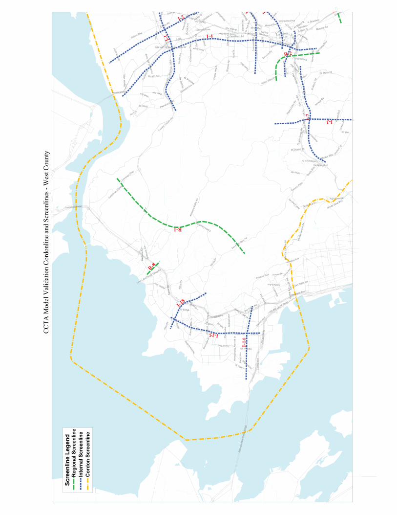
CCTA
Mod
el V
alid
atio
n Co
rdon
line
and
Scre
enlin
es -
Wes
t Cou
nty
I-4
R-1
I-7
I-15
I-14
R-2
I-18
R-8
I I
I-3
R
I-2
I-1
Wild
cat C
anyo
nRd
Franklin
Canyo
n Rd
San Pablo Dam Rd
Alha
mbr
aVa
lley
Rd
BearCree
kRd
SR24
Grizzly Peak Blvd
Ric
hmon
d/Sa
nR
afae
l Brid
ge
SR-4
Cummings Skwy
Benicia Bridge
Fish Ranch Rd
SR4
Solano Way
Moraga Rd
Imho
ffD
r
I-680
Stan
ley
Blvd
Richmon
dPkwy
South Park Dr
Mui
r Rd
Rhe
emBl
vd
Arlington Ave
Cumming
s Skyway
San Luis Rd
CastroRanchRd
Arno
ldD
r
SR242
Reliez Valley Rd
PalmAve
S. Broadway
Camino Pablo
Orcha
rdRd
Happ
y Valle
y Rd
Virg
inia
Hills
Dr
Taylor
Blvd
HallDr
MtD
iabl
oBl
vd
Cam
ino
Dia
blo
Tunn
elRd
Pleasant Hill Rd
Chi
lpan
cing
oPk
wy
Alhambra Ave
Carquinez Bridge
MinerRd
Wat
erfro
ntRd
Solano Wy
Morello Ave
Acalan
esRd
Oak
Park
Blvd
PasoNogal
Cen
ter A
ve
Oly
mpi
cBl
vd
CastroSt
Cleveland Ave
Olinda
Dr
St Stepens Dr
Arlington Blvd
St. Marys Rd
Mar
ina
Vist
a
Garrard
Blvd
Mine
rtRd
Appi
anW
y
Carlso
n Blvd
I-80
Homestead Ave
Gea
ryR
d
San Pablo AveTenant Ave/Pinole Valley Rd
ElN
ido
Ran
chR
d
I-80EBRam
p
Sunn
yval
eAv
e
Walnut Blvd
Hillt
opR
d
I-580 WB On/Off Ramp
AppianWay
I-680SB
Mcb
ryde
Ave
Gre
gory
Ln
Wild
Cat
Can
yon
Rd
Cu t
ting
Blv d
SR4 WB/ SB Ramp
I-580
EB
Ram
p
An Miguel Dr
JonesRd
Danville B
Vine
Hill
Wy
Moraga Way
ClaytonRd
I-80WBOnRamp
Terrace Dr
TiceVall
eyBlvd
Roa
d2 0
ShellAve
Colusa
Ave
Don
ald
Dr
Barre
ttAv
e
Mor
ago
Blvd
2nd
St
I-680 SB Ramp
NewellAve
Rob
ertH
Mil le
r Dr
23rd St
Grant St
Boyd
Rd
Cen
tralA
veSp
ringb
rook
Rd
Vikin
gDr
RumrillBlvd
Con
cord
Ave
Deer
Hill
Rd
Broadway
Rhe
em A
ve
AshburyAve
Santa Maria Dr
Bayb
erry
Ave
OrindawoodsDr
Carol Ln
I-80 WB RampSt
Mar
y'sR
d
Gol
fClu
bR
d
Hillto
pDr
San Pable Ave
OakRd
Burn
ettA
ve
Meadow Rd
Cleaveland Rd
Mt.Diab
loBlvd
Pach
eco
Dr
Buena Vista Ave
Alta
sRd
Oliv
era
Rd
Meadow Ln
Pach
eco/
I-680
Ram
p
Trea
tBlvd
ElPo
r tal D
r
May
hew
Wy
Gra
yson
Rd
BrownSt
Orinda
Way
23 Rd St
SierraLn
Civic Dr
Potre
roAv
e
BlumeDr
Bona
nzaStN. Broadway
LaCas
a V
ValeRd
S. Main St
ChurchLn
Raymond Dr
CherryLn
N.MainSt
HarbourWy
CurtolaBlvd
Broo
ksid
eDr
Syca
mor
eAv
e
Main St
ContraCostaBlvd
Market St
CogginsDrBuskirkAve
MacalveyDr
Fairm
ontA
ve
FerrySt
Moe
serL
n
Penn
sylv
ania
Ave
/13t
h St
Fry W
Monum
entB
l
Scre
enlin
e Le
gend
Regi
onal
Scr
eenl
ine
Inte
rnal
Scr
eenl
ine
Cord
on S
cree
nlin
e

CCTA
Mod
el V
alid
atio
n Co
rdon
line
and
Scre
enlin
es -
Cent
ral C
ount
y
I-4
R-4
R-1
I-1
I-5
I-3
I-7
I-6I-10
R-2
R-6
I-8R-5
R-3
R-8
R-7
I-2
Mt.DiabloScenicBlvd
Wild
cat C
anyo
nR
d
KirkerPassRd
Franklin
Canyo
n Rd
San Pablo Dam Rd
Marsh Cree
k Rd
Alha
mbr
aVa
lley
Rd
BearCreek
Rd
Pinehurst Rd
SR24
Grizzly Peak Blvd
SR-4
Cummings Skwy
Ston
eVa
lley
Rd
Rheem Blvd
Ygna
cioVa
lleyRd
SR4
Bailey
Rd
Blac
khaw
kD
r
Solano Way
Moraga Rd
Imho
ffD
r
I-680
Panoramic Drive
Stan
ley
Blvd
Skyline Blvd
Pitts
burg
-Ant
ioch
Hwy
Buch
anan
Bypa
ss
South Park Dr
Mui
r Rd
Blac
khaw
kRd
Arlington Ave
Avila
San Luis Rd
CastroRanchRd
Arno
ldD
r
Buch
a nan
Rd
Reliez Valley Rd
Dia
blo
Rd
PalmAve
S. Broadway
SLa
rwin
Ave
Camino Pablo
Orcha
rdRd
Happ
y Valle
y Rd MoragaRd(Moraga)
Virg
inia
Hills
Dr
TreatBlvd
Taylor
Blvd
HallDr
MtD
iabl
oBl
vd
Evo r
aR
d
SR242
Tunn
elRd
Pleasant Hill Rd
Chi
lpan
cing
oPk
wy
Green Valley Rd
Alhambra Ave
MinerRd
Wat
erfro
ntR
San Miguel Rd
Contra Loma Blvd
Camino
Tass
ajara
Solano Wy
Refu
gio
Valle
yRd
San Carlos Dr
RyanRd
Morello Ave
Acalan
esRd
ElPintadoRd
Cany
onRd
Concord Blvd
Nortonville Somersville Rd
Oak
Park
Blvd
PasoNogal
Donald Dr
Cen
ter A
ve
Oly
mpi
cB l
vd
SR4
WB
off-r
amp
Vent
ura
Dr
Olinda
Dr
St Stepens Dr
St. Marys Rd
WillowPassRd
SomersvilleRd
Fron
tage
Rd
Citrus Ave
Mar
ina
Vist
a
Cowe
ll Rd
Danville Blvd
Homestead Ave
Gea
ryR
d
Tent
hSt
SR 4 WB Ramp
SR4
EBR
amp
Walnut Blvd
Sprin
g bro
okR
d
PortChicagoHwy
Mine
rtRd W
alnut
Ave
Oak Grove Rd
Gre
gory
Ln
I-680 NB Off Ramp
Railroad Ave
Pennsylva
nia Blvd
SR4 WB/ SB Ramp
Lela
ndR
d
LavenderDr
N.La
rwin
Ave
An Miguel DrJonesRd
Sunn
yval
e Av
e
Palmer Rd
Harbor St
StM
ary's
Rd
MarketSt
Salvi
oSt
E.Le
land
Rd
Jam
esD
onlo
nD
r
ShellAveEl Cerro
Rd
Ced
roLn
Olive
Dr
Mor
ago
Blvd
I-680 SB Ramp
Clay
ton
Rd
NewellAve
San Jose Dr
Boyd
Rd
Vikin
gDr
2nd
Ave
San
Pabl
oAv
e
Santa Maria Dr
Carol Ln
Babel Lane
AlbertaWy
Gol
fClu
bR
d
Mou
ntai
nVi
ewBl
vd
Burn
ettA
ve
Ivy Dr
PinoleValleyRd
Meadow Rd
Pach
eco
Dr
CenturyBlvd
Buena Vista Ave
Mor
aga W
y
Meadow LnO
rinda
wood
sDr
ArthurRd
Gra
yson
Rd
BrownSt
RangeRd
SierraLn
Civic Dr
Trin
it yA v
e
Mt.
Dia
b lo
Blv d
FarmBureau Rd
Raymond Dr
CherryLn
Dee
rHill
Rd
ParksideDr
O St
Contra Costa Blvd
Bancroft Rd
Peralta Rd
Moraga Way
FerrySt
Syca
mor
eVa
lley
Rd
Fry WayGillDr
gs Skyway
Riftwo
Jam
esDo
n
nicia Bridge
lington Blvd
aBl
vd
saAve
Scre
enlin
e Le
gend
Regi
onal
Scr
eenl
ine
Inte
rnal
Scr
eenl
ine
Cord
on S
cree
nlin
e

CCTA
Mod
el V
alid
atio
n Co
rdon
line
and
Scre
enlin
es -
East
Coun
ty
I-13
R-4
I-12
I-10
R-6
3
R-5
SR 239
Mar
shCr
eek
Rd
Mt.DiabloScenicBlvd
KirkerPassRd
DeerValleyRd
Byron HwySR
-4
Ston
eVa
lley
Rd
Cam
ino
Dia
blo
Vasco
Rd
SR 4
Del
ta R
d
Ygna
cioVa
lleyRd
Balfo
ur R
d
Bailey
Rd
Che
stnu
tAve
Blac
khaw
kD
r
BixlerRd
Eure
ka A
ve
CM
Dia
blo
Panoramic Drive
Hol
e yR
d
Pitts
burg
-Ant
ioch
Hwy
Buch
anan
Bypa
ss
Blac
khaw
kR
d
Avila
BethelIslandRd
ByronSpringsRd
SellersAve
Buch
anan
Rd
Dia
b lo
Rd
Sandmound Blvd
Payn
eAv
e
SLa
rwin
Ave
Long
view
Rd
SR4 Bypass
San
Jose
Ave
TreatBlvd
PiperRd
Orw
ood
Rd
Arm
stro
ngR
d
Evor
aR
d
Green Valley Rd
Cent
ury
Blvd
San Miguel Rd
Contra Loma Blvd
Riftwood Dr Camino
Tass
ajara
WalnutBlvd
W. T
rega
llas
Rd
Poin
tofT
imbe
rRd
Sand
Cre
ekR
d
Tule
Ln
E .C
y pr e
s sR
d
RyanRd
N.L
arwi
nAv
e
ElPintadoRd
Neroly Rd
Bartels Dr
Concord Blvd
Jersey Island Rd
Nortonville Somersville Rd
W. S
and
Cre
ek R
d
Byer
Rd
FairviewAve
SR4
WB
off-r
amp
Vent
ura
Dr
Olivera Rd
Sellers
WillowPassRd
Concord Ave
SomersvilleRd
Fro n
tag e
Rd
Lone
Tree
Way
BigBreakRd
Citrus Ave
Boul
derD
r
Discovery Bay Blvd
Cowe
llRd
Empi
reM
ine
Rd
Fred
eric
kson
Ln
Dut
chSl
ough
Rd
Olive
Dr
Harbo
urDr
Tent
hSt
Rose Ave
Gat
eway
Rd
Cou
ntry
Hills
Dr
SR 4 WB Ramp
Hillcre
stAve
SR4
EBR
amp
tChicagoHwy
Waln
utAv
e
Blue
rock
Dr
Live Oak Ave
Suns
etD
r
Jam
esDo
nlon
Blvd
3rd
St
I-680 NB Off Ramp
Heidorn Ranch Rd
Syca
mor
eV a
lley
Rd
Mine
rtRd
Railroad Ave
Pennsylva
niaBlvd
Lela
ndR
d
Lark
spur
Dr
LavenderDr
Asilo
mar
Dr
MonumentBlvd
Palmer Rd
Harbor St
Creek Rd
G St
Mt D
iabl
oSt
18th
St
Shad
elan
dsDr
EmpireAve
Fulto
nSh
ipya
rdR
d
SR160NBRamp
Suns
etR
d
Gam
ayDr
Brow
n sto
neR
d
Danv
illeBl
vd
Texa
s St
Salvi
oSt
E.Le
land
Rd
Jam
esD
onlo
nD
r
Lone
Tre
e W
y
Ced
roLn
Mar
k Twa
inDr
Main St
Prew
ett R
anch
Dr
Minnesota Ave
MesaRidgeDr
Clay
ton
Rd
BarmouthDr
Wilb
urAv
e
Viera Ave
Whit
manRd
Bonf
icio
St
San Jose Dr
Trotter Wy
Cyp
ress
Dr
Bellflower Dr
I-680 SB Off Ramp
Brown RdCe
ntra
lBlvd
Brentwood Blvd
Rudgear Rd
D StSR160SBRamp
Babel Lane
AyersRd
Mar
ina
Blvd
AlbertaWy
ount
ain
View
Blvd
Sunset Ln
Dallas Ranch Rd
Dav
ison
Dr
Carp
inte
riaDr
Balfo
urD
r
LaurelRd
2nd St
10th
St
Eagl
erid
geD
r
Car
los
Dr
Indi
anHi
ll Dr
Range Rd
PutnamSt
Cen
tral A
ve
Blis
sAv
e
DeltaExpwy
Canada Valley Rd
ESa
nta
FeAv
e
O'HaraAve
6th
St
13th
St
FarmBureau Rd
GolfCo
urse
Rd
Via Dora Dr
NorcrossLn
O St
Knollcrest Dr
Love
ridge
Rd
Lone Oak Rd
Park
St
Syca
mo r
eAv
e
Parkside Dr
Ches
tnutS
t
Wild
Hor
se R
d
Mt Ham
ilton Dr
Fire Pl
San Ramon Rd
Grant S
t
orna
Rd
e
An
Casa Via
Scre
enlin
e Le
gend
Regi
onal
Scr
eenl
ine
Inte
rnal
Scr
eenl
ine
Cord
on S
cree
nlin
e

CCTA
Mod
el V
alid
atio
n Co
rdon
line
and
Scre
enlin
es -
Tri-V
alle
y
I-16
R-9
R-11
I-17
I-9
R-10
C-0
I-11
R-7
I-580
Vasc
oRd
Nile
sC
anyo
nR
d
Hig
h la n
dR
d
Crow
Canyo
nRd
I-680
N. Livermore Ave
Valle
citos
Rd
E. Bran
chRd
CollierCanyonRd
Alta
mon
t Pas
sRd
Vin e
y ar d
A ve
Norris
Canyo
nRd
Dub
linC
anyo
nR
d
Rte 84
Pleasanton Sunol
SR84
Stan
ley
Blvd
Greenville Rd
Bollinger Canyon Rd
NLivermoreAve
John
son
Dr
N.Fl
ynn
Rd
Paseo Santa Cruz
Tesl
a R
d
Rte24
Wet
mor
eR
d
El Capitan Dr
Mon
tevid
eoRd
CaminoTassajara
OldRanch
Rd
Laurel Creek Dr
San Ramon Valley Blvd
Tassajar
aRd
Stan
eley
Blvd
Tels
aR
d
Happ
yVa
lley
Rd
Shor
eline
Valle
y Av
e
N. Mines Rd
MONTEVIDEODR
Nor
thC
anyo
nsPk
wy
Muirwood Dr
Busc
hR
d
Pine
Valle
yRd
ArroyoRd
OldCrowCanyonRd
Win
derm
ere
Pkw
y
Isabel Ave
Vine
yar d
A ve/
Ra y
S t
Foothill Rd
Porto
laAv
e
East
Ave
Dougherty Rd
Holmes St
Murrie
taBl
vd
Liverm
oreAve
AlcostaBlvd
Ston
erid
geR
d
Syca
mor
eRd
Stanley
Ave
Crow Canyon Pl
SantaRita
Rd
Firs
tSt
Bern
alAv
e
W.L
asPo
sitas
Ave
I-680 SB Off Ramp
FallonRd
Payne Rd
SunolBlvd/FirstSt
Del V
alle
Pky
I-680 NB Off Ramp
DeerwoodDr
VillagePkwy
I-580
WB
Off R
amp
Greenwood Rd
GreenbrookDr
San Ramon Rd
HopyardRd
Ros
ewoo
d D
r
Camino Ramon
Mohr A
veKoll
n St
Rheem
Dr
I-580
EBOff R
amp
PleasantonAve
Fost
oria
Wy
Arno
ldR
dHaciendaDr
SunolBlvd
Gle
ason
Dr
Amador Plaza Rd
Owe
nsDr
El Charro Rd
Ange
laSt
Amad
orVa
lley
Blvd
Blackhawk Rd
Springdale Ave
Dubli
nBl
vd
Ston
erid
geD
r
Gib
ralta
r Dr
AirwayBlvd
Regional St
Koop
man
Broadmoor Dr
I-580
EBO
ffR
amp
ckhawk Dr
Patte
rson
Pass
Rd
Scre
enlin
e Le
gend
Regi
onal
Scr
eenl
ine
Inte
rnal
Scr
eenl
ine
Cord
on S
cree
nlin
e

Inte
rnal
Scr
eenl
ines
Peak
Hou
r Scr
eenl
ine
Ana
lysi
s - I
nter
nal S
cree
nlin
es
CC
TA M
odel
Doc
umen
tatio
n - A
ppen
dix
C
Scr
eenl
ine
IDS
cree
nlin
eS
tree
tL
egL
oca
tio
n20
00 C
nts
2000
Mo
del
% D
iff
2025
Mo
del
% G
row
th20
00 C
nts
2000
Mo
del
% D
iff
2025
Mo
del
% G
row
th14
7-N
BI
1SR
4A
lham
bra
SSR
444
832
5-2
7%82
115
3%53
745
3-1
6%1,
019
125%
148-
NB
I1
SR 4
Cen
ter
SM
uir
Roa
d31
118
7-4
0%20
39%
262
414
58%
531
28%
149-
NB
I1
SR 4
Mor
ello
Ave
nue
SM
uir
Roa
d45
149
510
%66
534
%73
645
9-3
8%62
636
%15
0-N
BI
1SR
4G
laci
er D
rive
SM
uir
Roa
d13
017
837
%23
834
%15
013
7-9
%20
046
%15
1-N
BI
1SR
4Pa
chec
o Bo
ulev
ard
SM
uir
Roa
d40
828
6-3
0%63
012
0%70
91,
123
58%
1,40
925
%15
2-N
BI
1SR
4I-6
80S
SR 4
4,94
14,
974
1%5,
560
12%
4,80
95,
711
19%
6,02
35%
153-
NB
I1
SR 4
Sola
no W
a yS
Oliv
era
173
79-5
4%36
035
6%14
567
-54%
144
115%
154-
NB
I1
SR 4
Oliv
era
SPe
ralta
132
478
262%
743
55%
118
265
125%
267
1%15
5-N
BI
1SR
4SR
242
NO
liver
a2,
669
2,23
3-1
6%3,
028
36%
3,74
85,
290
41%
6,23
918
%15
6-N
BI
1SR
4Po
rt C
hica
goS
SR 4
646
308
-52%
955
210%
541
723
34%
2,76
528
2%15
7-N
BI
1SR
4W
illow
Pas
sS
SR 4
673
352
-48%
171
-51%
1,27
495
5-2
5%1,
195
25%
Sub
tota
ls10
,982
9,89
5-1
0%13
,374
35%
13,0
2915
,597
20%
20,4
1831
%
147-
SBI
1SR
4A
lham
bra
SSR
439
062
360
%1,
310
110%
492
588
20%
1,00
771
%14
8-SB
I1
SR 4
Cen
ter
SM
uir
Roa
d27
946
266
%52
113
%26
026
42%
352
33%
149-
SBI
1SR
4M
orel
lo A
venu
eS
Mui
r R
oad
784
340
-57%
582
71%
775
618
-20%
703
14%
150-
SBI
1SR
4G
laci
er D
rive
SM
uir
Roa
d10
624
112
7%28
719
%13
918
332
%26
143
%15
1-SB
I1
SR 4
Pach
eco
Boul
evar
dS
Mui
r R
oad
465
1,12
014
1%1,
346
20%
521
448
-14%
1,53
024
2%15
2-SB
I1
SR 4
I-680
SSR
44,
962
6,22
826
%6,
913
11%
5,33
75,
027
-6%
5,58
811
%15
3-SB
I1
SR 4
Sola
no W
ayS
Oliv
era
159
54-6
6%55
793
1%17
119
212
%59
020
7%15
4-SB
I1
SR 4
Oliv
era
SPe
ralta
261
235
-10%
610
160%
146
762
422%
667
-12%
155-
SBI
1SR
4SR
242
NO
liver
a4,
104
4,81
917
%5,
841
21%
3,26
93,
389
4%3,
791
12%
156-
SBI
1SR
4Po
rt C
hica
goS
SR 4
450
1,07
713
9%2,
868
166%
902
384
-57%
1,16
720
4%15
7-SB
I1
SR 4
Will
ow P
ass
SSR
41,
025
1,01
8-1
%1,
395
37%
582
424
-27%
814
92%
Sub
tota
ls12
,985
16,2
1725
%22
,230
37%
12,5
9412
,279
-3%
16,4
7034
%T
ota
l23
,967
26,1
129%
35,6
0436
%25
,623
27,8
769%
36,8
8832
%
158-
EBI
2C
onco
rdW
ater
fron
tW
Sola
no18
415
-92%
1820
%43
4-9
1%8
100%
159-
EBI
2C
onco
rdIm
hoff
Dri
veE
Imho
ff12
418
-85%
5520
6%16
380
-51%
974
1118
%16
0-EB
I2
Con
cord
SR 4
EI-6
803,
058
3,00
3-2
%4,
289
43%
3,66
33,
804
4%4,
602
21%
161-
EBI
2C
onco
rdC
onco
rd A
venu
eE
J. G
len
836
196
-77%
296
51%
1,81
11,
587
-12%
2,01
327
%16
2-EB
I2
Con
cord
SR 2
42S
Con
cord
1,71
91,
951
13%
2,73
340
%5,
000
5,13
53%
5,84
414
%16
3-EB
I2
Con
cord
Mar
ket
Stre
etS
Con
cord
530
448
-15%
297
-34%
446
634
42%
545
-14%
164-
EBI
2C
onco
rdW
illow
Pas
s R
oad
EG
atew
ay48
880
365
%95
219
%94
61,
153
22%
1,41
423
%16
5-EB
I2
Con
cord
Cla
yton
Roa
dE
Gat
eway
738
925
25%
802
-13%
1,09
92,
058
87%
2,23
49%
166-
EBI
2C
onco
rdM
onum
ent
WC
owel
l70
91,
922
171%
2,34
222
%1,
600
1,30
0-1
9%1,
821
40%
167-
EBI
2C
onco
rdT
reat
Bou
leva
rdW
Cow
ell
563
328
-42%
422
29%
2,24
21,
743
-22%
1,77
32%
168-
EBI
2C
onco
rdY
gnai
co V
alle
yW
Lim
erid
ge63
849
1-2
3%70
143
%2,
926
2,11
2-2
8%3,
106
47%
Sub
tota
ls9,
587
10,1
005%
12,9
0728
%19
,939
19,6
10-2
%24
,334
24%
158-
WB
I2
Con
cord
Wat
erfr
ont
WSo
lano
433
-93%
610
0%12
38
-93%
1025
%15
9-W
BI
2C
onco
rdIm
hoff
Dri
veE
Imho
ff15
720
832
%1,
122
439%
120
22-8
2%71
223%
160-
WB
I2
Con
cord
SR 4
EI-6
804,
065
4,01
2-1
%4,
848
21%
3,18
72,
949
-7%
4,07
238
%16
1-W
BI
2C
onco
rdC
onco
rd A
venu
eE
J. G
len
1,71
72,
469
44%
2,79
713
%1,
336
573
-57%
824
44%
162-
WB
I2
Con
cord
SR 2
42S
Con
cord
5,00
04,
761
-5%
6,01
826
%2,
019
3,40
168
%4,
736
39%
163-
WB
I2
Con
cord
Mar
ket
Stre
etS
Con
cord
530
320
-40%
199
-38%
446
410
-8%
184
-55%
164-
WB
I2
Con
cord
Will
ow P
ass
Roa
dE
Gat
eway
565
1,69
320
0%1,
684
-1%
611
1,17
993
%1,
375
17%
165-
WB
I2
Con
cord
Cla
yton
Roa
dE
Gat
eway
983
1,75
979
%2,
020
15%
942
425
-55%
471
11%
166-
WB
I2
Con
cord
Mon
umen
tW
Cow
ell
1,31
481
3-3
8%1,
800
121%
1,05
01,
431
36%
2,03
642
%16
7-W
BI
2C
onco
rdT
reat
Bou
leva
rdW
Cow
ell
2,15
41,
944
-10%
1,99
43%
776
663
-15%
812
22%
168-
WB
I2
Con
cord
Ygn
aico
Val
ley
WLi
mer
idge
2,91
22,
230
-23%
3,35
751
%86
51,
021
18%
1,40
237
%-
Sub
tota
ls19
,440
20,2
124%
25,8
4528
%11
,475
12,0
825%
15,9
9332
%T
ota
l29
,027
30,3
124%
38,7
5228
%31
,414
31,6
921%
40,3
2727
%- 16
9-EB
I3
Ori
nda
Hap
p y V
alle
yE
Upp
er H
appy
Val
ley
218
156
-28%
205
31%
115
178
55%
667
275%
170-
EBI
3O
rind
aSR
24
EEl
Nid
o5,
700
5,31
3-7
%9,
064
71%
7,82
67,
930
1%9,
573
21%
171-
EBI
3O
rind
aM
t. D
iabl
oE
El N
ido
565
104
-82%
268
158%
778
1,38
778
%2,
009
45%
172-
EBI
3O
rind
aR
heem
Val
ley
EZ
ande
r63
224
256%
238
6%15
731
910
3%42
032
%17
3-EB
I3
Ori
nda
Mor
aga
Way
EIv
y D
rive
166
185
11%
218
18%
425
300
-29%
342
14%
-S
ubto
tals
6,71
25,
982
-11%
9,99
367
%9,
301
10,1
149%
13,0
1129
%- 16
9-W
BI
3O
rind
aH
appy
Val
ley
EU
pper
Hap
py V
alle
y19
821
06%
635
202%
128
176
38%
292
66%
170-
WB
I3
Ori
nda
SR 2
4E
El N
ido
8,58
78,
413
-2%
10,1
7921
%5,
342
5,65
86%
7,82
538
%17
1-W
BI
3O
rind
aM
t. D
iabl
oE
El N
ido
613
1,99
522
5%2,
586
30%
741
761
3%1,
295
70%
172-
WB
I3
Ori
nda
Rhe
em V
alle
yE
Zan
der
121
341
182%
459
35%
123
270
120%
350
30%
173-
WB
I3
Ori
nda
Mor
aga
Way
EIv
y D
rive
292
230
-21%
290
26%
252
250
-1%
361
44%
-S
ubto
tals
9,81
111
,189
14%
14,1
4926
%6,
586
7,11
58%
10,1
2342
%T
ota
l16
,523
17,1
714%
24,1
4241
%15
,887
17,2
298%
23,1
3434
%-
AM
Pea
k H
our
PM
Pea
k H
our
1 of
68/
9/20
06

Inte
rnal
Scr
eenl
ines
Peak
Hou
r Scr
eenl
ine
Ana
lysi
s - I
nter
nal S
cree
nlin
es
CC
TA M
odel
Doc
umen
tatio
n - A
ppen
dix
C
Scr
eenl
ine
IDS
cree
nlin
eS
tree
tL
egL
oca
tio
n20
00 C
nts
2000
Mo
del
% D
iff
2025
Mo
del
% G
row
th20
00 C
nts
2000
Mo
del
% D
iff
2025
Mo
del
% G
row
thA
M P
eak
Ho
urP
M P
eak
Ho
ur
174-
EBI
4I-6
80M
arin
a V
ista
WI-6
8029
532
19%
668
108%
644
612
-5%
712
16%
175-
EBI
4I-6
80Pa
chec
oW
I-680
Ram
ps82
544
9-4
6%49
19%
958
386
-60%
866
124%
176-
EBI
4I-6
80A
rnol
d D
rive
WPa
chec
o11
928
-76%
106
279%
8319
-77%
124
553%
177-
EBI
4I-6
80SR
4W
Pach
eco
3,95
02,
805
-29%
3,54
326
%3,
745
3,40
0-9
%4,
481
32%
178-
EBI
4I-6
80M
uir
Roa
dW
SR 4
Ram
ps52
456
27%
579
3%37
632
3-1
4%32
1-1
%17
9-EB
I4
I-680
Cen
ter
Stre
etE
Ray
mon
d25
132
931
%23
2-2
9%27
925
9-7
%30
719
%18
0-EB
I4
I-680
Chi
lpac
ingo
WPa
chec
o79
873
3-8
%1,
099
50%
666
768
15%
1,13
448
%18
1-EB
I4
I-680
Gol
f Clu
bE
Old
Qua
r30
821
0-3
2%62
819
9%55
329
-95%
5910
3%18
2-EB
I4
I-680
Vik
ing
ER
uth
293
103
-65%
89-1
4%40
748
419
%49
83%
183-
EBI
4I-6
80T
aylo
rE
Rut
h79
585
78%
1,50
375
%45
91,
296
182%
1,81
240
%18
4-EB
I4
I-680
Boyd
Roa
dE
Putn
am69
153
5-2
3%72
135
%43
143
10%
523
21%
185-
EBI
4I-6
80G
rego
ryE
Elin
ora
679
588
-13%
792
35%
1,00
648
4-5
2%68
642
%18
6-EB
I4
I-680
Sunn
yval
eW
N. M
ain
165
358
117%
319
-11%
8527
622
5%26
2-5
%18
7-EB
I4
I-680
Oak
Par
kW
Plea
sant
Val
ley
Dr
678
334
-51%
647
94%
321
260
-19%
398
53%
188-
EBI
4I-6
80G
ear y
Roa
dE
Buen
a72
456
3-2
2%78
239
%61
128
5-5
3%28
60%
189-
EBI
4I-6
802n
d S
tree
tW
N. M
ain
104
170
63%
265
56%
8022
818
5%20
4-1
1%19
0-EB
I4
I-680
San
Luis
WI-6
80 R
amps
441
605
37%
682
13%
212
330
56%
416
26%
191-
EBI
4I-6
80Bu
ena
Vis
taW
I-680
460
871
89%
1,07
824
%15
544
518
7%67
151
%19
2-EB
I4
I-680
Spri
ngbk
WC
amin
o45
167
271%
164
-2%
7512
972
%21
264
%19
3-EB
I4
I-680
SR 2
4W
I-680
5,90
85,
948
1%7,
825
32%
9,31
18,
993
-3%
11,2
0925
%30
9-EB
I4
I-680
Boul
evar
d W
ayE
Sara
nap
Ave
203
139
-32%
198
42%
279
199
-29%
294
48%
194-
EBI
4I-6
80O
lym
pic
ET
ice
Val
ley
Blvd
829
622
-25%
623
0%99
11,
023
3%1,
319
29%
-S
ubto
tals
19,0
8517
,297
-9%
23,0
3433
%21
,727
20,6
59-5
%26
,794
30%
- 174-
WB
I4
I-680
Mar
ina
Vis
taW
I-680
641
851
33%
875
3%36
347
731
%69
546
%17
5-W
BI
4I-6
80Pa
chec
oE
Mor
ello
891
324
-64%
663
105%
1,95
341
1-7
9%51
726
%17
6-W
BI
4I-6
80A
rnol
d D
rive
WPa
chec
o10
442
-60%
9813
3%17
267
-61%
293
337%
177-
WB
I4
I-680
SR 4
WPa
chec
o3,
238
3,30
12%
2,35
5-2
9%4,
435
2,84
2-3
6%2,
122
-25%
178-
WB
I4
I-680
Mui
r R
oad
WSR
4 R
amps
224
233
4%18
9-1
9%26
537
742
%27
5-2
7%17
9-W
BI
4I-6
80C
ente
r St
reet
ER
a ym
ond
154
111
-28%
215
94%
247
330
34%
171
-48%
180-
WB
I4
I-680
Chi
lpac
ingo
WPa
chec
o81
663
9-2
2%92
745
%61
178
228
%1,
001
28%
181-
WB
I4
I-680
Gol
f Clu
bE
Old
Qua
r36
819
-95%
7127
4%71
219
6-7
2%64
422
9%18
2-W
BI
4I-6
80V
ikin
gE
Rut
h20
562
920
7%55
5-1
2%39
014
5-6
3%16
111
%18
3-W
BI
4I-6
80T
aylo
rE
Rut
h1,
009
1,27
226
%1,
527
20%
1,12
71,
008
-11%
1,72
571
%18
4-W
BI
4I-6
80Bo
yd R
oad
EPu
tnam
262
370
41%
443
20%
404
570
41%
736
29%
185-
WB
I4
I-680
Gre
gory
EEl
inor
a90
939
2-5
7%48
022
%65
369
56%
837
20%
186-
WB
I4
I-680
Sunn
yval
eW
N. M
ain
6018
120
2%17
8-2
%13
352
029
1%51
80%
187-
WB
I4
I-680
Oak
Par
kW
Plea
sant
Val
ley
Dr
361
149
-59%
281
89%
586
218
-63%
573
163%
188-
WB
I4
I-680
Gea
ry R
oad
EBu
ena
506
152
-70%
194
28%
735
560
-24%
886
58%
189-
WB
I4
I-680
2nd
Str
eet
WN
. Mai
n46
178
287%
178
0%96
261
172%
409
57%
190-
WB
I4
I-680
San
Luis
WI-6
80 R
amps
171
165
-4%
171
4%34
152
755
%55
76%
191-
WB
I4
I-680
Buen
a V
ista
WI-6
8043
712
9-7
0%64
540
0%46
384
983
%1,
038
22%
192-
WB
I4
I-680
Spri
ngbk
WC
amin
o80
8810
%17
810
2%62
183
195%
196
7%19
3-W
BI
4I-6
80SR
24
WI-6
808,
485
8,93
05%
10,6
2119
%6,
782
6,70
6-1
%8,
719
30%
309-
WB
I4
I-680
Boul
evar
d W
ayE
Sara
nap
Ave
272
144
-47%
195
35%
290
201
-31%
333
66%
194-
WB
I4
I-680
Oly
mpi
cE
Tic
e V
alle
y Bl
vd1,
048
864
-18%
965
12%
1,07
499
7-7
%1,
079
8%-
Sub
tota
ls20
,287
19,1
63-6
%22
,004
15%
21,8
9418
,922
-14%
23,4
8524
%T
ota
l39
,372
36,4
60-7
%45
,038
24%
43,6
2139
,581
-9%
50,2
7927
%- 19
5-N
BI
5T
reat
Ta y
lor
SW
ither
s35
936
41%
1,26
724
8%1,
258
1,23
5-2
%1,
886
53%
196-
NB
I5
Tre
atPl
easa
ntN
Gea
ry34
411
2-6
7%25
112
4%57
531
7-4
5%79
615
1%19
7-N
BI
5T
reat
Putn
am B
oule
vard
NG
eary
402
234
-42%
838
258%
517
994
92%
1,08
69%
198-
NB
I5
Tre
atM
ain
Stre
etN
Gea
ry1,
129
342
-70%
984
188%
1,27
01,
816
43%
2,04
613
%19
9-N
BI
5T
reat
I-680
NT
reat
7,52
58,
041
7%9,
649
20%
10,4
949,
816
-6%
11,2
3314
%20
0-N
BI
5T
reat
Busk
irk
NT
reat
1,24
81,
048
-16%
1,16
011
%1,
733
1,47
6-1
5%1,
540
4%20
1-N
BI
5T
reat
Oak
Roa
dN
Tre
at44
547
06%
593
26%
598
1,32
512
2%1,
984
50%
202-
NB
I5
Tre
atC
oggi
ns L
ane
NT
reat
942
60-9
4%20
424
0%29
349
970
%71
243
%20
3-N
BI
5T
reat
Che
rry
Lane
NT
reat
8742
739
1%60
341
%13
661
134
9%67
310
%20
4-N
BI
5T
reat
Banc
roft
NT
reat
411
646
57%
551
-15%
738
749
1%87
917
%20
5-N
BI
5T
reat
Oak
Gro
veN
Tre
at99
969
4-3
1%1,
243
79%
1,18
21,
320
12%
1,54
617
%20
6-N
BI
5T
reat
Cow
ell
Roa
dN
Tre
at82
659
8-2
8%86
745
%69
529
2-5
8%36
124
%20
7-N
BI
5T
reat
Cla
yton
Roa
dW
Den
king
e1,
486
2,34
258
%3,
328
42%
971
696
-28%
992
43%
-S
ubto
tals
16,2
0315
,378
-5%
21,5
3840
%20
,460
21,1
463%
25,7
3422
%- 19
5-SB
I5
Tre
atT
aylo
rS
With
ers
1,59
21,
429
-10%
1,82
628
%54
288
363
%1,
420
61%
196-
SBI
5T
reat
Plea
san t
NG
eary
581
373
-36%
804
116%
305
233
-24%
462
98%
197-
SBI
5T
reat
Putn
am B
oule
vard
NG
eary
655
1,01
154
%1,
148
14%
405
663
64%
912
38%
198-
SBI
5T
reat
Mai
n St
reet
NG
eary
1,34
62,
875
114%
3,51
122
%1,
219
1,57
329
%1,
853
18%
199-
SBI
5T
reat
I-680
NT
reat
9,62
010
,526
9%10
,967
4%7,
876
8,89
713
%9,
508
7%20
1-SB
I5
Tre
atO
ak R
oad
NT
reat
816
531
-35%
396
-25%
744
217
-71%
418
93%
202-
SBI
5T
reat
Cog
gins
NT
reat
300
551
84%
679
23%
632
116
-82%
132
14%
203-
SBI
5T
reat
Che
rry
Lane
NT
reat
212
520
145%
704
35%
111
509
359%
587
15%
204-
SBI
5T
reat
Banc
roft
NT
reat
1,26
793
5-2
6%91
2-2
%66
871
27%
857
20%
205-
SBI
5T
reat
Oak
Gro
veN
Tre
at84
41,
433
70%
1,59
311
%99
51,
275
28%
1,68
532
%20
6-SB
I5
Tre
atC
owel
l Roa
dN
Tre
at52
620
2-6
2%19
0-6
%1,
071
517
-52%
756
46%
207-
SBI
5T
reat
Cla
yton
Roa
dW
Den
king
e73
948
0-3
5%74
355
%1,
812
1,81
50%
2,87
558
%-
Sub
tota
ls18
,498
20,8
6613
%23
,473
12%
16,3
8017
,410
6%21
,465
23%
To
tal
34,7
0136
,244
4%45
,011
24%
36,8
4038
,556
5%47
,199
22%
2 of
68/
9/20
06

Inte
rnal
Scr
eenl
ines
Peak
Hou
r Scr
eenl
ine
Ana
lysi
s - I
nter
nal S
cree
nlin
es
CC
TA M
odel
Doc
umen
tatio
n - A
ppen
dix
C
Scr
eenl
ine
IDS
cree
nlin
eS
tree
tL
egL
oca
tio
n20
00 C
nts
2000
Mo
del
% D
iff
2025
Mo
del
% G
row
th20
00 C
nts
2000
Mo
del
% D
iff
2025
Mo
del
% G
row
thA
M P
eak
Ho
urP
M P
eak
Ho
ur
208-
NB
I6
Ygn
acio
Banc
roft
NY
gnac
io96
299
13%
1,24
225
%1,
163
1,31
013
%1,
580
21%
209-
NB
I6
Ygn
acio
Cal
iforn
iaN
Ygn
acio
661
819
24%
1,14
840
%87
11,
596
83%
1,93
121
%21
0-N
BI
6Y
gnac
ioC
ivic
Dri
veN
Ygn
acio
748
455
-39%
653
44%
962
949
-1%
1,66
375
%21
1-N
BI
6Y
gnac
ioI-6
80N
Ygn
acio
7,37
18,
140
10%
9,68
619
%9,
475
10,4
8311
%11
,229
7%21
2-N
BI
6Y
gnac
ioM
ain
Stre
etN
Ygn
acio
550
565
3%97
973
%96
988
1-9
%1,
787
103%
213-
NB
I6
Ygn
acio
N. B
road
way
NY
gnac
io29
443
347
%54
726
%51
936
3-3
0%52
444
%21
4-N
BI
6Y
gnac
ioO
ak G
rove
NY
gnac
io1,
670
633
-62%
1,05
967
%99
01,
242
25%
984
-21%
215-
NB
I6
Ygn
acio
Wal
nut
Boul
evar
dN
Ygn
acio
352
261
-26%
447
71%
209
514
146%
597
16%
-S
ubto
tals
12,6
0812
,297
-2%
15,7
6128
%15
,158
17,3
3814
%20
,295
17%
- 208-
SBI
6Y
gnac
ioBa
ncro
ftN
Ygn
acio
1,43
01,
287
-10%
1,37
87%
1,08
61,
283
18%
1,42
511
%20
9-SB
I6
Ygn
acio
Cal
iforn
iaN
Ygn
acio
983
1,39
442
%1,
784
28%
1,12
797
3-1
4%1,
573
62%
210-
SBI
6Y
gnac
ioC
ivic
Dri
veN
Ygn
acio
1,04
71,
043
0%1,
552
49%
900
585
-35%
924
58%
211-
SBI
6Y
gnac
ioI-6
80N
Ygn
acio
10,1
3711
,070
9%12
,131
10%
9,20
58,
860
-4%
10,5
0019
%21
2-SB
I6
Ygn
acio
Mai
n St
reet
NY
gnac
io1,
089
909
-17%
1,35
149
%88
893
86%
1,44
554
%21
3-SB
I6
Ygn
acio
N. B
road
way
NY
gnac
io58
080
-86%
471
489%
523
124
-76%
490
295%
214-
SBI
6Y
gnac
ioO
ak G
rove
NY
gnac
io85
21,
063
25%
731
-31%
1,00
41,
014
1%1,
516
50%
215-
SBI
6Y
gnac
ioW
alnu
t Bo
ulev
ard
NY
gnac
io34
649
844
%52
45%
198
479
142%
446
-7%
-S
ubto
tals
16,4
6417
,344
5%19
,922
15%
14,9
3114
,256
-5%
18,3
1929
%T
ota
l29
,072
29,6
412%
35,6
8320
%30
,089
31,5
945%
38,6
1422
%- 21
6-N
BI
7SR
24
Aca
lane
sS
Mt.
Dia
blo
189
748
296%
984
32%
149
632
324%
793
25%
217-
NB
I7
SR 2
4M
orag
a R
oad
SM
t. D
iabl
o1,
128
816
-28%
1,32
763
%1,
001
708
-29%
944
33%
218-
NB
I7
SR 2
4M
orag
a W
ayW
Cam
ino
Pabl
o97
075
8-2
2%87
716
%55
155
20%
661
20%
219-
NB
I7
SR 2
4Pl
easa
nt H
illS
Mt.
Dia
blo
849
832
-2%
898
8%82
555
9-3
2%51
0-9
%-
Sub
tota
ls3,
136
3,15
41%
4,08
630
%2,
526
2,45
1-3
%2,
908
19%
- 216-
SBI
7SR
24
Aca
lane
sS
Mt.
Dia
blo
109
335
207%
383
14%
248
743
200%
1,01
036
%21
7-SB
I7
SR 2
4M
orag
a R
oad
SM
t. D
iabl
o82
669
6-1
6%1,
121
61%
959
842
-12%
1,64
295
%21
8-SB
I7
SR 2
4M
orag
a W
ayW
Cam
ino
Pabl
o63
838
7-3
9%39
21%
1,17
689
5-2
4%96
98%
219-
SBI
7SR
24
Plea
sant
Hill
SM
t. D
iabl
o64
730
1-5
3%28
3-6
%80
877
8-4
%74
6-4
%-
Sub
tota
ls2,
220
1,71
9-2
3%2,
179
27%
3,19
13,
258
2%4,
367
34%
To
tal
5,35
64,
873
-9%
6,26
529
%5,
717
5,70
90%
7,27
527
%- 22
0-N
BI
8W
alnu
t C
reek
Plea
sant
Hill
ND
eer
Hill
713
510
-28%
1,64
022
2%2,
013
2,15
07%
2,89
134
%22
1-N
BI
8W
alnu
t C
reek
I-680
NSR
24
7,37
18,
140
10%
9,68
619
%9,
475
10,4
8311
%11
,229
7%22
2-N
BI
8W
alnu
t C
reek
Oak
land
Ave
NM
t. D
iabl
o18
129
-84%
4659
%28
716
2-4
4%31
997
%31
0-N
BI
8W
alnu
t C
reek
Bona
nza
StN
Mt.
Dia
blo
351
0-1
00%
412
343
16-9
5%44
426
75%
223-
NB
I8
Wal
nut
Cre
ekC
alifo
rnia
NM
t. D
iabl
o68
674
89%
740
-1%
1,06
31,
678
58%
1,76
25%
224-
NB
I8
Wal
nut
Cre
ekN
. Mai
n St
reet
NM
t. D
iabl
o52
367
-87%
470
601%
439
134
-69%
637
375%
225-
NB
I8
Wal
nut
Cre
ekBr
oadw
a yN
Mt.
Dia
blo
638
1,23
694
%2,
054
66%
1,29
61,
270
-2%
1,77
139
%22
6-N
BI
8W
alnu
t C
reek
Wal
nut
BdS
Ygn
acio
213
648
204%
687
6%29
865
512
0%61
8-6
%22
7-N
BI
8W
alnu
t C
reek
Hom
este
adS
Ygn
acio
434
62-8
6%22
826
8%34
818
1-4
8%53
519
6%-
Sub
tota
ls11
,110
11,4
403%
15,9
6340
%15
,562
16,7
297%
20,2
0621
%- 22
0-SB
I8
Wal
nut
Cre
ekPl
easa
nt H
illN
Dee
r H
ill1,
974
2,23
813
%2,
834
27%
846
1,23
045
%1,
996
62%
221-
SBI
8W
alnu
t C
reek
I-680
NSR
24
10,7
3712
,743
19%
13,7
628%
9,80
511
,628
19%
15,1
9731
%22
2-SB
I8
Wal
nut
Cre
ekO
akla
nd A
veN
Mt.
Dia
blo
435
468
8%56
922
%44
721
0-5
3%48
413
0%31
0-SB
I8
Wal
nut
Cre
ekBo
nanz
a St
NM
t. D
iabl
o22
52
-99%
514
2560
0%34
01
-100
%50
450
300%
223-
SBI
8W
alnu
t C
reek
Cal
iforn
iaN
Mt.
Dia
blo
707
1,41
810
1%1,
483
5%73
51,
055
44%
1,48
941
%22
4-SB
I8
Wal
nut
Cre
ekN
. Mai
n St
reet
NM
t. D
iabl
o52
365
-88%
793
1120
%43
910
4-7
6%74
261
3%22
5-SB
I8
Wal
nut
Cre
ekBr
oadw
ayN
Mt.
Dia
blo
1,05
41,
326
26%
1,78
134
%1,
022
1,36
433
%2,
102
54%
226-
SBI
8W
alnu
t C
reek
Wal
nut
BdS
Ygn
acio
450
574
28%
633
10%
385
746
94%
729
-2%
227-
SBI
8W
alnu
t C
reek
Hom
este
adS
Ygn
acio
250
44-8
2%21
238
2%28
655
-81%
139
153%
-S
ubto
tal s
16,3
5518
,878
15%
22,5
8120
%14
,305
16,3
9315
%23
,382
43%
To
tal
27,4
6530
,318
10%
38,5
4427
%29
,867
33,1
2211
%43
,588
32%
- 228-
NB
I9
San
Ram
onI-6
80S
Bolli
nger
5,76
05,
632
-2%
5,62
10%
6,27
06,
645
6%6,
003
-10%
229-
NB
I9
San
Ram
onSa
n R
amon
Val
ley
SBo
lling
er1,
229
780
-37%
1,15
148
%77
880
53%
1,74
911
7%23
0-N
BI
9Sa
n R
amon
Alc
osta
SBo
lling
er1,
139
849
-25%
1,41
266
%66
554
6-1
8%1,
229
125%
-S
ubto
tals
8,12
87,
261
-11%
8,18
413
%7,
713
7,99
64%
8,98
112
%- 22
8-SB
I9
San
Ram
onI-6
80S
Bolli
nger
5,46
26,
723
23%
6,46
2-4
%5,
913
6,44
89%
5,94
4-8
%22
9-SB
I9
San
Ram
onSa
n R
amon
Val
ley
SBo
lling
er64
150
9-2
1%1,
829
259%
1,16
285
3-2
7%1,
840
116%
230-
SBI
9Sa
n R
amon
Alc
osta
SBo
lling
er54
841
4-2
4%1,
120
171%
1,15
51,
020
-12%
1,57
755
%-
Sub
tota
ls6,
651
7,64
615
%9,
411
23%
8,23
08,
321
1%9,
361
12%
To
tal
14,7
7914
,907
1%17
,595
18%
15,9
4316
,317
2%18
,342
12%
-
3 of
68/
9/20
06

Inte
rnal
Scr
eenl
ines
Peak
Hou
r Scr
eenl
ine
Ana
lysi
s - I
nter
nal S
cree
nlin
es
CC
TA M
odel
Doc
umen
tatio
n - A
ppen
dix
C
Scr
eenl
ine
IDS
cree
nlin
eS
tree
tL
egL
oca
tio
n20
00 C
nts
2000
Mo
del
% D
iff
2025
Mo
del
% G
row
th20
00 C
nts
2000
Mo
del
% D
iff
2025
Mo
del
% G
row
thA
M P
eak
Ho
urP
M P
eak
Ho
ur
231-
EBI
10D
anvi
lleSt
one
Val
ley
EM
iran
da65
698
951
%1,
173
19%
705
697
-1%
838
20%
232-
EBI
10D
anvi
lleEl
Cer
roE
El P
inta
377
756
101%
1,34
678
%50
317
1-6
6%29
170
%23
3-EB
I10
Dan
ville
Dia
blo
Roa
dE
I-680
1,07
11,
231
15%
2,28
886
%72
785
718
%82
8-3
%32
0-EB
I10
Dan
ville
Syca
mor
e V
alle
y R
oad
EI-6
8071
51,
131
58%
1,93
171
%1,
463
1,46
60%
2,31
058
%S
ubto
tals
2,81
94,
107
46%
6,73
864
%3,
398
3,19
1-6
%4,
267
34%
- 231-
WB
I10
Dan
ville
Ston
e V
alle
yE
Mir
anda
808
867
7%98
313
%70
678
611
%1,
069
36%
232-
WB
I10
Dan
ville
El C
erro
EEl
Pin
ta76
214
1-8
1%17
323
%51
966
628
%1,
096
65%
233-
WB
I10
Dan
ville
Dia
blo
Roa
dE
I-680
892
596
-33%
594
0%1,
562
1,25
3-2
0%2,
163
73%
320-
WB
I10
Dan
ville
Syca
mor
e V
alle
y R
oad
EI-6
801,
721
1,40
7-1
8%2,
189
56%
1,05
61,
110
5%1,
623
46%
-S
ubto
tals
4,18
33,
011
-28%
3,93
931
%3,
843
3,81
5-1
%5,
951
56%
To
tal
7,00
27,
118
2%10
,677
50%
7,24
17,
006
-3%
10,2
1846
%- 23
4-EB
I11
Dan
ville
Blac
khaw
kE
Mt.
Dia
blo
425
383
-10%
838
119%
427
704
65%
1,09
656
%23
5-EB
I11
Dan
ville
Cam
ino
Tas
sE
S yca
mor
e83
876
8-8
%1,
007
31%
1,43
81,
648
15%
3,05
285
%35
3-EB
I11
Dan
ville
Cro
w C
anyo
nE
Alc
osta
648
399
-38%
628
57%
2,14
01,
930
-10%
2,73
542
%35
4-EB
I11
Dan
ville
Bolli
nger
E
Alc
osta
419
250
-40%
861
244%
841
1,07
127
%2,
843
165%
-S
ubto
tals
2,33
01,
800
-23%
3,33
485
%4,
846
5,35
310
%9,
726
82%
- 234-
WB
I11
Dan
ville
Blac
khaw
kE
Mt.
Dia
blo
686
684
0%1,
091
60%
370
452
22%
689
52%
235-
WB
I11
Dan
ville
Cam
ino
Tas
sE
Syca
mor
e1,
615
1,40
3-1
3%3,
158
125%
970
949
-2%
1,15
321
%35
3-W
BI
11D
anvi
lleC
row
Can
yon
EA
lcos
ta2,
169
1,98
9-8
%3,
001
51%
1,00
379
4-2
1%1,
255
58%
354-
WB
I11
Dan
ville
Bolli
nger
E
Alc
ost a
764
1,07
941
%2,
633
144%
478
491
3%1,
590
224%
-S
ubto
tals
5,23
45,
155
-2%
9,88
392
%2,
821
2,68
6-5
%4,
687
74%
To
tal
7,56
46,
955
-8%
13,2
1790
%7,
667
8,03
95%
14,4
1379
%- 23
6-N
BI
12A
ntio
ch/B
rent
woo
dLo
ne T
ree
SJa
mes
Don
lon
Blvd
1,24
82,
116
70%
3,37
559
%1,
224
1,21
4-1
%1,
745
44%
237-
NB
I12
Ant
ioch
/Bre
ntw
ood
Hill
cres
tN
Lone
Tre
e48
286
279
%27
2-6
8%55
179
144
%26
5-6
6%23
8-N
BI
12A
ntio
ch/B
rent
woo
dR
oute
4 B
ypas
sN
Lone
Tre
e41
175
239-
NB
I12
Ant
ioch
/Bre
ntw
ood
Empi
reN
Lone
Tre
e21
925
014
%34
237
%42
338
3-9
%41
58%
240-
NB
I12
Ant
ioch
/Bre
ntw
ood
SR 4
Eas
tN
Lone
Tre
e65
832
6-5
0%36
010
%68
254
3-2
0%88
763
%24
1-N
BI
12A
ntio
ch/B
rent
woo
dSe
llers
SD
elta
198
25-8
7%19
266
8%17
366
-62%
346
424%
242-
NB
I12
Ant
ioch
/Bre
ntw
ood
B yro
n H
ighw
ayS
Del
ta83
437
5-5
5%36
-90%
536
445
-17%
145
-67%
243-
NB
I12
Ant
ioch
/Bre
ntw
ood
O'H
ara
NLo
ne T
ree
110
37-6
6%14
428
9%19
042
-78%
258
514%
341-
NB
I12
Ant
ioch
/Bre
ntw
ood
Kni
ghts
en A
ve15
1134
2-N
BI
12A
ntio
ch/B
rent
woo
dLo
ne T
ree
Way
Ext
n0
234
3-N
BI
12A
ntio
ch/B
rent
woo
dA
nder
son
Ln0
334
5-N
BI
12A
ntio
ch/B
rent
woo
dH
ighw
a y 4
Foo
tage
Rd
149
346-
NB
I12
Ant
ioch
/Bre
ntw
ood
Futu
re R
d94
146
347-
NB
I12
Ant
ioch
/Bre
ntw
ood
Cou
ntry
Hill
s D
rV
iste
Gra
nde
Ave
22
348-
NB
I12
Ant
ioch
/Bre
ntw
ood
Vis
te G
rand
e A
ve16
1334
9-N
BI
12A
ntio
ch/B
rent
woo
dD
eer
Val
ley
Rd
547
269
350-
NB
I12
Ant
ioch
/Bre
ntw
ood
Cou
ntry
Hill
s D
rLo
ne T
ree
104
133
351-
NB
I12
Ant
ioch
/Bre
ntw
ood
Eagl
erid
ge D
r19
835
2-N
BI
12A
ntio
ch/B
rent
woo
dBl
uero
ak D
r16
137
-S
ubto
tal s
3,74
93,
991
6%5,
734
44%
3,77
93,
484
-8%
4,86
940
%- 23
6-SB
I12
Ant
ioch
/Bre
ntw
ood
Lone
Tre
eS
Jam
es D
onlo
n Bl
vd84
647
7-4
4%77
262
%1,
051
2,12
710
2%3,
290
55%
237-
SBI
12A
ntio
ch/B
rent
woo
dH
illcr
est
NLo
ne T
ree
524
767
46%
267
-65%
688
915
33%
480
-48%
238-
SBI
12A
ntio
ch/B
rent
woo
dR
oute
4 B
ypas
sN
Lone
Tre
e14
210
623
9-SB
I12
Ant
ioch
/Bre
ntw
ood
Empi
reN
Lone
Tre
e33
329
0-1
3%25
4-1
2%34
436
25%
515
42%
240-
SBI
12A
ntio
ch/B
rent
woo
dSR
4 E
ast
NLo
ne T
ree
504
511
1%75
347
%81
840
3-5
1%60
951
%24
1-SB
I12
Ant
ioch
/Bre
ntw
ood
Selle
rsS
Del
ta11
648
-59%
330
588%
287
36-8
7%27
566
4%24
2-SB
I12
Ant
ioch
/Bre
ntw
ood
Byro
n H
ighw
ayS
Del
ta48
944
7-9
%14
5-6
8%77
148
9-3
7%88
-82%
243-
SBI
12A
ntio
ch/B
rent
woo
dO
'Har
aN
Lone
Tre
e16
624
-86%
196
717%
180
61-6
6%22
426
7%34
1-SB
I12
Ant
ioch
/Bre
ntw
ood
Kni
ghts
en A
ve8
2334
2-SB
I12
Ant
ioch
/Bre
ntw
ood
Lone
Tre
e W
a y E
xtn
20
343-
SBI
12A
ntio
ch/B
rent
woo
dA
nder
son
Ln1
134
5-SB
I12
Ant
ioch
/Bre
ntw
ood
Hig
hway
4 F
oota
ge R
d3
1734
6-SB
I12
Ant
ioch
/Bre
ntw
ood
Futu
re R
d12
715
934
7-SB
I12
Ant
ioch
/Bre
ntw
ood
Cou
ntry
Hill
s D
rV
iste
Gra
nde
Ave
22
348-
SBI
12A
ntio
ch/B
rent
woo
dV
iste
Gra
nde
Ave
721
349-
SBI
12A
ntio
ch/B
rent
woo
dD
eer
Val
ley
Rd
479
784
350-
SBI
12A
ntio
ch/B
rent
woo
dC
ount
ry H
ills
Dr
Lone
Tre
e66
189
351-
SBI
12A
ntio
ch/B
rent
woo
dEa
gler
idge
Dr
416
352-
SBI
12A
ntio
ch/B
rent
woo
dBl
uero
ak D
r30
143
-S
ubto
tal s
2,97
82,
564
-14%
3,58
840
%4,
139
4,39
36%
6,94
258
%T
ota
l6,
727
6,55
5-3
%9,
322
42%
7,91
87,
877
-1%
11,8
1150
%-
4 of
68/
9/20
06

Inte
rnal
Scr
eenl
ines
Peak
Hou
r Scr
eenl
ine
Ana
lysi
s - I
nter
nal S
cree
nlin
es
CC
TA M
odel
Doc
umen
tatio
n - A
ppen
dix
C
Scr
eenl
ine
IDS
cree
nlin
eS
tree
tL
egL
oca
tio
n20
00 C
nts
2000
Mo
del
% D
iff
2025
Mo
del
% G
row
th20
00 C
nts
2000
Mo
del
% D
iff
2025
Mo
del
% G
row
thA
M P
eak
Ho
urP
M P
eak
Ho
ur
244-
EBI
13O
akle
y/Br
entw
ood
SR 4
ESR
160
1,09
485
8-2
2%99
616
%1,
888
2,20
817
%2,
203
0%24
5-EB
I13
Oak
ley/
Bren
twoo
dLo
ne T
ree
EH
illcr
est
799
1,12
641
%67
4-4
0%96
71,
688
75%
2,12
126
%24
6-EB
I13
Oak
ley/
Bren
twoo
dBa
lfour
ED
eer
Val
ley
937
143
-85%
205
43%
1,00
759
3-4
1%59
0-1
%24
7-EB
I13
Oak
ley/
Bren
twoo
dM
arsh
Cre
ekE
Dee
r V
alle
y14
946
-69%
17-6
3%31
245
947
%50
811
%32
1-EB
I13
Oak
ley/
Bren
twoo
dR
oute
4 B
ypas
s1,
754
4,13
333
0-EB
I13
Oak
ley/
Bren
twoo
dW
ilbur
Ave
474
402
331-
EBI
13O
akle
y/Br
entw
ood
Oak
ley
Ave
4320
733
2-EB
I13
Oak
ley/
Bren
twoo
dH
ighw
ay 4
Foo
tage
Rd
349
633
3-EB
I13
Oak
ley/
Bren
twoo
dW
ild H
orse
Rd
185
503
334-
EBI
13O
akle
y/Br
entw
ood
Laur
el R
d28
710
033
6-EB
I13
Oak
ley/
Bren
twoo
dC
ount
ry H
ills
Dr
1041
337-
EBI
13O
akle
y/Br
entw
ood
Vis
te G
rand
e A
ve8
2533
8-EB
I13
Oak
ley/
Bren
twoo
dPr
ewet
t R
anch
Dr
203
332
339-
EBI
13O
akle
y/Br
entw
ood
Sand
Cre
ek R
d19
860
034
0-EB
I13
Oak
ley/
Bren
twoo
dH
illcr
est
Ave
1478
-S
ubto
tals
2,97
92,
173
-27%
5,07
113
3%4,
174
4,94
819
%12
,339
149%
- 244-
WB
I13
Oak
ley/
Bren
twoo
dSR
4E
SR 1
601,
467
2,23
853
%2,
063
-8%
1,25
31,
345
7%1,
273
-5%
245-
WB
I13
Oak
ley/
Bren
twoo
dLo
ne T
ree
EH
illcr
est
835
1,58
490
%1,
646
4%95
41,
278
34%
870
-32%
246-
WB
I13
Oak
ley/
Bren
twoo
dBa
lfour
ED
eer
Val
ley
778
485
-38%
548
13%
1,02
621
2-7
9%39
385
%24
7-W
BI
13O
akle
y/Br
entw
ood
Mar
sh C
reek
ED
eer
Val
ley
353
471
33%
525
11%
132
75-4
3%28
-63%
321-
WB
I13
Oak
ley/
Bren
twoo
dR
oute
4 B
ypas
s4,
485
2,43
933
0-W
BI
13O
akle
y/Br
entw
ood
Wilb
ur A
ve35
945
533
1-W
BI
13O
akle
y/Br
entw
ood
Oak
ley
Ave
389
7233
2-W
BI
13O
akle
y/Br
entw
ood
Hig
hway
4 F
oota
ge R
d42
215
333-
WB
I13
Oak
ley/
Bren
twoo
dW
ild H
orse
Rd
359
248
334-
WB
I13
Oak
ley/
Bren
twoo
dLa
urel
Rd
6136
333
6-W
BI
13O
akle
y/Br
entw
ood
Cou
ntry
Hill
s D
r32
1733
7-W
BI
13O
akle
y/Br
entw
ood
Vis
te G
rand
e A
ve11
1833
8-W
BI
13O
akle
y/Br
entw
ood
Prew
ett
Ran
ch D
r17
231
033
9-W
BI
13O
akle
y/Br
entw
ood
Sand
Cre
ek R
d31
746
034
0-W
BI
13O
akle
y/Br
entw
ood
Hill
cres
t A
ve60
52-
Sub
tota
ls3,
433
4,77
839
%11
,449
140%
3,36
52,
910
-14%
7,01
314
1%T
ota
l6,
412
6,95
18%
16,5
2013
8%7,
539
7,85
84%
19,3
5214
6%- 24
8-N
BI
14R
ichm
ond
Cas
tro
NI-5
8069
834
3-5
1%45
633
%1,
767
899
-49%
2,06
012
9%24
9-N
BI
14R
ichm
ond
Gar
rard
SM
acD
onal
d18
014
8-1
8%30
310
5%42
033
2-2
1%54
163
%25
0-N
BI
14R
ichm
ond
Har
bour
SM
acD
onal
d42
033
5-2
0%44
031
%62
141
2-3
4%61
249
%25
1-N
BI
14R
ichm
ond
23rd
Str
eet
SM
acD
onal
d26
938
744
%76
197
%1,
287
1,06
5-1
7%1,
919
80%
252-
NB
I14
Ric
hmon
dI-8
0S
Mac
Don
ald
4,96
84,
393
-12%
5,44
424
%7,
838
10,1
0229
%10
,948
8%25
3-N
BI
14R
ichm
ond
San
Pabl
oS
Mac
Don
ald
856
146
-83%
403
176%
1,75
81,
339
-24%
1,78
033
%-
Sub
tota
ls7,
391
5,75
2-2
2%7,
807
36%
13,6
9114
,149
3%17
,860
26%
- 248-
SBI
14R
ichm
ond
Cas
tro
NI-5
801,
732
1,60
0-8
%1,
928
21%
724
246
-66%
618
151%
249-
SBI
14R
ichm
ond
Gar
rard
SM
acD
onal
d35
742
218
%1,
259
198%
220
243
10%
477
96%
250-
SBI
14R
ichm
ond
Har
bour
SM
acD
onal
d50
957
313
%1,
704
197%
479
564
18%
738
31%
251-
SBI
14R
ichm
ond
23rd
Str
eet
SM
acD
onal
d1,
186
1,71
945
%1,
989
16%
391
798
104%
1,35
870
%25
2-SB
I14
Ric
hmon
dI-8
0S
Mac
Don
ald
8,11
710
,172
25%
11,2
3010
%4,
597
5,92
829
%6,
276
6%25
3-SB
I14
Ric
hmon
dSa
n Pa
blo
SM
acD
onal
d1,
884
1,54
7-1
8%1,
847
19%
1,41
845
0-6
8%1,
317
193%
-S
ubto
tals
13,7
8516
,033
16%
19,9
5724
%7,
829
8,22
95%
10,7
8431
%T
ota
l21
,176
21,7
853%
27,7
6427
%21
,520
22,3
784%
28,6
4428
%- 25
4-EB
I15
Ric
h/Sa
npb
Ric
hmon
d Pa
rkw
ayE
San
Pabl
o90
264
7-2
8%70
39%
1,40
81,
116
-21%
2,43
411
8%25
5-EB
I15
Ric
h/Sa
npb
Hill
top
ESa
n Pa
blo
232
154
-34%
169
10%
433
125
-71%
369
195%
256-
EBI
15R
ich/
Sanp
bR
H M
iller
ESa
n Pa
blo
217
166
-24%
205
23%
490
243
-50%
379
56%
257-
EBI
15R
ich/
Sanp
bEl
Por
tal
ESa
n Pa
blo
533
397
-26%
463
17%
599
280
-53%
430
54%
258-
EBI
15R
ich/
Sanp
bR
oad
20E
San
Pabl
o13
515
515
%93
-40%
224
160
-29%
382
139%
311-
EBI
15R
ich/
Sanp
bSa
n Pa
blo
Ave
E23
rd S
t44
339
2-1
2%96
914
7%48
11,
671
247%
2,08
725
%31
2-EB
I15
Ric
h/Sa
npb
Mar
ket
Ave
E23
rd S
t38
431
7-1
7%38
421
%53
524
9-5
3%26
04%
259-
EBI
15R
ich/
Sanp
bR
heem
Bou
leva
rdE
23rd
St
321
174
-46%
239
37%
404
411
2%24
9-3
9%31
3-EB
I15
Ric
h/Sa
npb
Mcb
ryde
Ave
E23
rd S
t88
49-4
4%36
-27%
103
153
49%
113
-26%
260-
EBI
15R
ich/
Sanp
bBa
rret
Ave
nue
E23
rd S
t43
340
7-6
%26
3-3
5%77
041
0-4
7%73
479
%26
1-EB
I15
Ric
h/Sa
npb
Mac
Don
ald
E23
rd S
t46
110
0-7
8%99
-1%
634
121
-81%
154
27%
262-
EBI
15R
ich/
Sanp
bC
uttin
gE
23rd
St
590
364
-38%
547
50%
691
381
-45%
619
62%
105-
EB15
Ric
h/Sa
npb
Ric
hmon
d/Sa
n R
afae
l Bri
dge
2,32
62,
582
11%
2,45
1-5
%2,
757
1,70
1-3
8%2,
640
55%
-S
ubto
tals
7,06
55,
904
-16%
6,62
112
%9,
529
7,02
1-2
6%10
,850
55%
- 254-
WB
I15
Ric
h/Sa
npb
Ric
hmon
d Pa
rkw
ayE
San
Pabl
o1,
404
1,68
720
%3,
446
104%
1,04
481
4-2
2%1,
479
82%
255-
WB
I15
Ric
h/Sa
npb
Hill
top
ESa
n Pa
blo
210
68-6
8%16
914
9%38
616
7-5
7%25
050
%25
6-W
BI
15R
ich/
Sanp
bR
H M
iller
ESa
n Pa
blo
307
158
-49%
227
44%
642
259
-60%
294
14%
257-
WB
I15
Ric
h/Sa
npb
El P
orta
lE
San
Pabl
o37
519
4-4
8%24
928
%46
842
7-9
%53
626
%25
8-W
BI
15R
ich/
Sanp
bR
oad
20E
San
Pabl
o10
162
-39%
282
355%
165
108
-35%
89-1
8%31
1-W
BI
15R
ich/
Sanp
bSa
n Pa
blo
Ave
E23
rd S
t36
01,
606
346%
2,08
030
%76
267
1-1
2%1,
617
141%
312-
WB
I15
Ric
h/Sa
npb
Mar
ket
Ave
E23
rd S
t40
320
2-5
0%25
024
%46
440
8-1
2%30
5-2
5%25
9-W
BI
15R
ich/
Sanp
bR
heem
Bou
leva
rdE
23rd
St
337
402
19%
425
6%37
435
7-5
%30
8-1
4%31
3-W
BI
15R
ich/
Sanp
bM
cbry
de A
veE
23rd
St
102
191
87%
105
-45%
106
117
10%
72-3
8%26
0-W
BI
15R
ich/
Sanp
bBa
rret
Ave
nue
E23
rd S
t57
945
7-2
1%51
613
%46
232
3-3
0%39
121
%26
1-W
BI
15R
ich/
Sanp
bM
acD
onal
dE
23rd
St
509
104
-80%
278
167%
650
172
-74%
229
33%
262-
WB
I15
Ric
h/Sa
npb
Cut
ting
E23
rd S
t85
246
0-4
6%68
950
%74
449
1-3
4%92
889
%10
5-W
BI
15R
ich/
Sanp
bR
ichm
ond/
San
Raf
ael B
ridg
e3,
514
3,39
5-3
%5,
112
51%
2,79
34,
337
55%
4,40
11%
-S
ubto
tals
9,05
38,
986
-1%
13,8
2854
%9,
060
8,65
1-5
%10
,899
26%
To
tal
16,1
1814
,890
-8%
20,4
4937
%18
,589
15,6
72-1
6%21
,749
39%
-
5 of
68/
9/20
06

Inte
rnal
Scr
eenl
ines
Peak
Hou
r Scr
eenl
ine
Ana
lysi
s - I
nter
nal S
cree
nlin
es
CC
TA M
odel
Doc
umen
tatio
n - A
ppen
dix
C
Scr
eenl
ine
IDS
cree
nlin
eS
tree
tL
egL
oca
tio
n20
00 C
nts
2000
Mo
del
% D
iff
2025
Mo
del
% G
row
th20
00 C
nts
2000
Mo
del
% D
iff
2025
Mo
del
% G
row
thA
M P
eak
Ho
urP
M P
eak
Ho
ur
263-
NB
I16
I-580
San
Ram
on R
oad
ND
ublin
Blv
d84
264
5-2
3%1,
554
141%
1,44
22,
199
52%
3,08
240
%26
4-N
BI
16I-5
80R
egio
nal S
tree
t N
Dub
lin B
lvd
234
101
-57%
411
307%
408
77-8
1%57
865
1%26
5-N
BI
16I-5
80A
mad
or P
laza
ND
ublin
Blv
d14
869
-53%
65-6
%31
832
42%
261
-19%
266-
NB
I16
I-580
I-680
N
Dub
lin B
lvd
5,75
95,
150
-11%
5,83
013
%6,
269
6,05
8-3
%7,
149
18%
267-
NB
I16
I-580
Vill
age
Pkw
yN
Dub
lin B
lvd
394
269
-32%
421
57%
799
1,08
336
%1,
957
81%
268-
NB
I16
I-580
Dou
gher
t y
ND
ublin
Blv
d1,
696
699
-59%
1,30
487
%1,
363
1,54
313
%2,
291
48%
269-
NB
I16
I-580
Hac
iend
a D
rive
ND
ublin
Blv
d86
939
6-5
4%89
012
5%45
530
8-3
2%63
710
7%27
0-N
BI
16I-5
80T
assa
jara
Roa
dN
Dub
lin B
lvd
521
83-8
4%52
653
4%68
831
9-5
4%2,
929
818%
271-
NB
I16
I-580
Fallo
n N
I-580
478
-83%
638
7875
%20
3050
%2,
143
7043
%27
2-N
BI
16I-5
80C
ollie
r C
anyo
n N
Can
yon
Pkw
y74
817
1004
%1,
008
23%
106
130
23%
1,06
772
1%27
3-N
BI
16I-5
80N
. Liv
erm
ore
NI-5
8011
316
748
%77
236
2%26
281
-69%
1,52
117
78%
274-
NB
I16
I-580
Vas
co
SSc
enic
792
826
4%1,
089
32%
1,58
11,
006
-36%
1,42
642
%-
Sub
tota
ls11
,489
9,23
0-2
0%14
,508
57%
13,7
1113
,158
-4%
25,0
4190
%- 26
3-SB
I16
I-580
San
Ram
on R
oad
ND
ublin
Blv
d1,
552
2,35
752
%3,
289
40%
1,21
91,
262
4%1,
349
7%26
4-SB
I16
I-580
Reg
iona
l Str
eet
ND
ublin
Blv
d29
465
-78%
208
220%
415
107
-74%
358
235%
265-
SBI
16I-5
80A
mad
or P
laza
ND
ublin
Blv
d12
029
814
8%15
4-4
8%25
720
7-1
9%16
6-2
0%26
6-SB
I16
I-580
I-680
N
Dub
lin B
lvd
5,46
15,
749
5%8,
498
48%
5,91
25,
466
-8%
7,43
736
%26
7-SB
I16
I-580
Vill
age
Pkw
yN
Dub
lin B
lvd
668
1,40
111
0%1,
940
38%
722
801
11%
1,15
044
%26
8-SB
I16
I-580
Dou
gher
ty
ND
ublin
Blv
d94
81,
301
37%
2,44
388
%1,
486
716
-52%
1,21
169
%26
9-SB
I16
I-580
Hac
iend
a D
rive
ND
ublin
Blv
d47
920
9-5
6%38
886
%84
837
1-5
6%82
612
3%27
0-SB
I16
I-580
Tas
saja
ra R
oad
ND
ublin
Blv
d79
737
6-5
3%2,
904
672%
597
113
-81%
1,00
679
0%27
1-SB
I16
I-580
Fallo
n N
I-580
2710
-63%
1,64
816
380%
3412
-65%
1,00
482
67%
272-
SBI
16I-5
80C
ollie
r C
anyo
n N
Can
yon
Pkw
y67
55-1
8%96
416
53%
121
761
529%
1,15
151
%27
3-SB
I16
I-580
N. L
iver
mor
e N
I-580
716
35-9
5%1,
438
4009
%22
736
862
%1,
095
198%
274-
SBI
16I-5
80V
asco
S
Scen
ic1,
321
1,30
8-1
%1,
686
29%
958
962
0%1,
368
42%
-S
ubto
tals
12,4
5013
,164
6%25
,560
94%
12,7
9611
,146
-13%
18,1
2163
%T
ota
l23
,939
22,3
94-6
%40
,068
79%
26,5
0724
,304
-8%
43,1
6278
%- 27
5-EB
I17
Wes
t Li
verm
ore
I-580
E
El C
harr
o5,
711
7,14
525
%7,
876
10%
8,61
79,
834
14%
10,7
119%
276-
EBI
17W
est
Live
rmor
eSt
anle
y Bl
vdE
El C
harr
o52
147
7-8
%54
314
%2,
428
1,98
1-1
8%1,
882
-5%
277-
EBI
17W
est
Live
rmor
eV
iney
ard
Ave
WIs
abel
Ave
154
33-7
9%80
142%
798
935
17%
827
-12%
278-
EBI
17W
est
Live
rmor
eR
te 8
4 S
Vin
eyar
d A
ve46
451
311
%45
9-1
1%1,
536
987
-36%
816
-17%
-S
ubto
tals
6,85
08,
168
19%
8,95
810
%13
,379
13,7
373%
14,2
364%
- 275-
WB
I17
Wes
t Li
verm
ore
I-580
E
El C
harr
o10
,324
9,06
5-1
2%9,
010
-1%
6,28
67,
290
16%
7,58
74%
276-
WB
I17
Wes
t Li
verm
ore
Stan
ley
Blvd
EEl
Cha
rro
1,97
51,
935
-2%
1,83
5-5
%65
196
148
%1,
346
40%
277-
WB
I17
Wes
t Li
verm
ore
Vin
eyar
d A
veW
Isab
el A
ve36
360
867
%52
7-1
3%16
278
-52%
232
197%
278-
WB
I17
Wes
t Li
verm
ore
Rte
84
SV
ine y
ard
Ave
974
937
-4%
788
-16%
537
890
66%
341
-62%
-S
ubto
tals
13,6
3612
,545
-8%
12,1
60-3
%7,
636
9,21
921
%9,
506
3%T
ota
l20
,486
20,7
131%
21,1
182%
21,0
1522
,956
9%23
,742
3%- 31
4-EB
I18
Pino
le/C
ount
yR
ichm
ond
Pkw
yS
Atla
s R
d81
332
0-6
1%66
010
6%2,
292
1,21
3-4
7%3,
261
169%
315-
EBI
18Pi
nole
/Cou
nty
San
Pabl
o A
veN
Hill
top
Dr
520
342
-34%
1,10
822
4%94
21,
542
64%
1,88
522
%31
6-EB
I18
Pino
le/C
ount
yH
illto
p D
rE
I-80
695
122
-82%
165
35%
934
424
-55%
1,53
526
2%31
7-N
BI
18Pi
nole
/Cou
nty
App
ian
Way
NSa
n Pa
blo
Dam
Rd
381
185
-51%
531
187%
641
599
-7%
1,01
569
%31
8-EB
I18
Pino
le/C
ount
ySa
n Pa
blo
Dam
Rd
EA
ppia
n W
ay93
967
2-2
8%77
716
%1,
216
1,49
923
%1,
903
27%
319-
EBI
18Pi
nole
/Cou
nty
I-80
NH
illto
p D
r4,
734
4,87
53%
6,25
128
%6,
664
9,57
944
%10
,647
11%
-S
ubto
tal s
8,08
26,
516
-19%
9,49
246
%12
,689
14,8
5617
%20
,246
36%
- 314-
WB
I18
Pino
le/C
ount
yR
ichm
ond
Pkw
yS
Atla
s R
d1,
935
2,00
54%
4,06
410
3%69
841
0-4
1%1,
079
163%
315-
WB
I18
Pino
le/C
ount
ySa
n Pa
blo
Ave
NH
illto
p D
r81
91,
548
89%
1,98
328
%69
357
4-1
7%1,
734
202%
316-
WB
I18
Pino
le/C
ount
yH
illto
p D
rE
I-80
888
497
-44%
1,77
425
7%59
225
1-5
8%32
529
%31
7-SB
I18
Pino
le/C
ount
yA
ppia
n W
ayN
San
Pabl
o D
am R
d57
060
15%
698
16%
490
331
-32%
749
126%
318-
WB
I18
Pino
le/C
ount
ySa
n Pa
blo
Dam
Rd
EA
ppia
n W
ay1,
371
1,61
218
%2,
117
31%
1,05
488
1-1
6%1,
035
17%
319-
WB
I18
Pino
le/C
ount
yI-8
0N
Hill
top
Dr
7,03
69,
789
39%
10,5
558%
4,97
75,
764
16%
6,69
516
%S
ubto
tals
12,6
1916
,052
27%
21,1
9132
%8,
504
8,21
1-3
%11
,617
41%
To
tal
20,7
0122
,568
9%30
,683
36%
21,1
9323
,067
9%31
,863
38%
2792
Gra
nd T
ota
l35
0,38
735
5,96
72%
476,
452
34%
374,
190
380,
833
2%51
0,60
034
%
6 of
68/
9/20
06

Reg
iona
l Scr
eenl
ines
Peak
Hou
r Scr
eenl
ine
Ana
lysi
s - R
egio
nal S
cree
nlin
es
CC
TA M
odel
Doc
umen
tatio
n - A
ppen
dix
C
Scr
eenl
ine
IDN
OS
cree
nlin
eS
tree
tL
egL
oca
tio
n20
00 C
nts
2000
Mo
del
% D
iff
2025
Mo
del
% G
row
th20
00 C
nts
2000
Mo
del
% D
iff
2025
Mo
del
% G
row
th10
0-N
BC
0C
ordo
n Li
neBy
ron
Hig
hway
Ala
med
a C
o61
759
6-3
%1,
106
86%
551
743
35%
921
24%
101-
WB
C0
Cor
don
Line
SR 4
San
Joaq
uin
Co
338
302
-11%
452
50%
245
271
11%
405
49%
102-
SBC
0C
ordo
n Li
neA
ntio
ch B
ridg
eSa
cram
ento
Co
509
351
-31%
980
179%
438
569
30%
948
67%
103-
SBC
0C
ordo
n Li
neBe
nici
a Br
idge
Sola
no C
o4,
347
5,37
724
%7,
062
31%
3,90
44,
299
10%
5,71
933
%10
4-SB
C0
Cor
don
Line
Car
quin
ez B
ridg
eSo
lano
Co
6,90
87,
838
13%
9,93
927
%6,
941
5,19
0-2
5%7,
812
51%
105-
EBC
0C
ordo
n Li
neR
ichm
ond/
San
Raf
ael B
ridg
eM
arin
Co
2,32
62,
582
11%
2,45
1-5
%2,
757
1,70
1-3
8%2,
640
55%
106-
SBC
0C
ordo
n Li
neI-5
80 s
/o C
entr
alA
lam
eda
Co
2,30
91,
968
-15%
2,98
752
%3,
669
4,36
419
%4,
816
10%
107-
SBC
0C
ordo
n Li
neI-8
0 s/
o C
entr
alA
lam
eda
Co
7,49
86,
409
-15%
7,34
615
%7,
494
4,85
4-3
5%5,
638
16%
108-
NB
C0
Cor
don
Line
San
Pabl
o A
venu
eA
lam
eda
Co
646
161
-75%
322
100%
1,34
21,
854
38%
1,96
36%
109-
NB
C0
Cor
don
Line
Arl
ingt
onA
lam
eda
Co
775
25-9
7%29
16%
981
431
-56%
752
74%
110-
NB
C0
Cor
don
Line
Wild
cat
Can
yon
Ala
med
a C
o62
254
310%
461
81%
8440
-52%
8912
3%11
1-EB
C0
Cor
don
Line
Lom
as C
onta
dis
Ala
med
a C
o13
249
1815
%42
571
%31
9-7
1%52
478%
112-
EBC
0C
ordo
n Li
neSR
24
Cal
Ala
med
a C
o3,
638
3,86
96%
6,17
760
%8,
452
8,76
54%
10,6
6722
%11
3-N
BC
0C
ordo
n Li
nePi
nehu
rst
Roa
dA
lam
eda
Co
4052
30%
137
163%
5314
016
4%29
110
8%11
4-EB
C0
Cor
don
Line
Cro
w C
anyo
n R
oad
Ala
med
a C
o94
269
8-2
6%1,
071
53%
910
790
-13%
997
26%
115-
EBC
0C
ordo
n Li
neN
orri
s C
anyo
n R
oad
Ala
med
a C
o22
042
593
%65
855
%13
714
99%
372
150%
116-
NB
C0
Cor
don
Line
San
Ram
on V
alle
y Bl
vdA
lam
eda
Co
678
372
-45%
1,11
019
8%97
51,
303
34%
2,14
064
%11
7-N
BC
0C
ordo
n Li
neI-6
80 V
alle
y S.
A.
Ala
med
a C
o5,
759
5,15
0-1
1%5,
830
13%
6,26
96,
058
-3%
7,14
918
%30
0-N
BC
0C
ordo
n Li
neV
illag
e Pk
wy
Ala
med
a C
o32
919
2-4
2%25
332
%48
577
860
%1,
142
47%
118-
NB
C0
Cor
don
Line
Dou
gher
ty R
oad
Ala
med
a C
o1,
525
141
-91%
469
233%
1,22
591
3-2
5%2,
566
181%
301-
NB
C0
Cor
don
Line
Tas
saja
ra R
dA
lam
eda
Co
184
10-9
5%53
652
60%
573
291
-49%
2,42
473
3%30
2-W
BC
0C
ordo
n Li
neN
. Liv
erm
ore
Ave
Ala
med
a C
o63
42-3
3%53
211
67%
1510
-33%
161
1510
%11
9-N
BC
0C
ordo
n Li
neV
asco
Roa
dA
lam
eda
Co
672
738
10%
886
20%
1,30
188
0-3
2%98
512
%-
Sub
tota
ls40
,398
37,6
09-7
%50
,966
36%
48,8
3244
,402
-9%
60,6
4937
%- 10
0-SB
C0
Cor
don
Line
Byro
n H
ighw
ayA
lam
eda
Co
665
861
29%
1,12
931
%37
664
371
%1,
047
63%
101-
EBC
0C
ordo
n Li
neSR
4Sa
n Jo
aqui
n C
o24
125
66%
383
50%
339
366
8%54
749
%10
2-N
BC
0C
ordo
n Li
neA
ntio
ch B
ridg
eSa
cram
ento
Co
382
472
24%
816
73%
656
516
-21%
983
91%
103-
NB
C0
Cor
don
Line
Beni
cia
Brid
geSo
lano
Co
3,12
23,
927
26%
5,51
140
%4,
294
4,71
610
%5,
456
16%
104-
NB
C0
Cor
don
Line
Car
quin
ez B
ridg
eSo
lano
Co
6,72
85,
300
-21%
8,03
952
%7,
723
7,66
9-1
%10
,099
32%
105-
WB
C0
Cor
don
Line
Ric
hmon
d/Sa
n R
afae
l Bri
dge
Mar
in C
o3,
514
3,39
5-3
%5,
112
51%
2,79
34,
337
55%
4,40
11%
106-
NB
C0
Cor
don
Line
I-580
s/o
Cen
tral
Ala
med
a C
o3,
545
4,09
215
%4,
801
17%
3,16
42,
579
-18%
3,71
344
%10
7-N
BC
0C
ordo
n Li
neI-8
0 s/
o C
entr
alA
lam
eda
Co
4,87
83,
659
-25%
4,76
530
%5,
033
6,56
931
%7,
626
16%
108-
SBC
0C
ordo
n Li
neSa
n Pa
blo
Ave
nue
Ala
med
a C
o1,
430
1,82
728
%1,
967
8%99
91,
372
37%
1,77
429
%10
9-SB
C0
Cor
don
Line
Arl
ingt
onA
lam
eda
Co
415
613
48%
799
30%
764
133
-83%
254
91%
110-
SBC
0C
ordo
n Li
neW
ildca
t C
anyo
nA
lam
eda
Co
545
-91%
1928
0%11
615
534
%24
759
%11
1-W
BC
0C
ordo
n Li
neLo
mas
Con
tadi
sA
lam
eda
Co
2921
-28%
9334
3%24
140
483%
648
363%
112-
WB
C0
Cor
don
Line
SR 2
4 C
alA
lam
eda
Co
10,7
199,
715
-9%
10,9
4613
%4,
727
5,07
27%
7,72
752
%11
3-SB
C0
Cor
don
Line
Pine
hurs
t R
oad
Ala
med
a C
o68
227
234%
381
68%
103
114
11%
210
84%
114-
WB
C0
Cor
don
Line
Cro
w C
anyo
n R
oad
Ala
med
a C
o86
085
2-1
%97
815
%1,
052
689
-35%
1,03
550
%11
5-W
BC
0C
ordo
n Li
neN
orri
s C
anyo
n R
oad
Ala
med
a C
o16
410
7-3
5%26
314
6%15
024
966
%36
547
%11
6-SB
C0
Cor
don
Line
San
Ram
on V
alle
y Bl
vdA
lam
eda
Co
756
1,46
994
%2,
127
45%
670
944
41%
1,00
67%
117-
SBC
0C
ordo
n Li
neI-6
80 V
alle
y S.
A.
Ala
med
a C
o5,
461
5,74
95%
8,49
848
%5,
912
5,46
6-8
%7,
437
36%
300-
SBC
0C
ordo
n Li
neV
illag
e Pk
wy
SA
lam
eda
Co
358
1,05
119
4%1,
559
48%
465
528
14%
582
10%
118-
SBC
0C
ordo
n Li
neD
ough
erty
Roa
dA
lam
eda
Co
851
944
11%
2,87
620
5%1,
335
416
-69%
873
110%
301-
SBC
0C
ordo
n Li
neT
assa
jara
Rd
NA
lam
eda
Co
498
360
-28%
2,40
856
9%22
329
-87%
845
2814
%30
2-EB
C0
Cor
don
Line
N. L
iver
mor
e A
veN
Ala
med
a C
o10
9-1
0%69
667%
319
244
-24%
740
203%
119-
SBC
0C
ordo
n Li
neV
asco
Roa
dA
lam
eda
Co
976
921
-6%
1,10
120
%69
779
314
%89
913
%-
Ala
med
a31
,737
32,4
822%
44,7
7938
%26
,129
26,1
350%
37,0
2842
%So
lano
9,85
09,
227
-6%
13,5
5047
%12
,017
12,3
853%
15,5
5526
%M
arin
3,51
43,
395
-3%
5,11
251
%2,
793
4,33
755
%4,
401
1%-
Sub
tota
ls45
,724
44,7
81-2
%63
,081
41%
41,9
3443
,739
4%58
,514
34%
To
tal
45,0
5976
,509
70%
105,
414
38%
90,7
6688
,141
-3%
119,
163
35%
- 120-
EBR
1W
est/
Cen
tral
Cum
min
gs S
kyw
ay W
. SR
4W
SR 4
881
372
-58%
227
-39%
209
290
39%
225
-22%
121-
EBR
1W
est/
Cen
tral
SR 4
WC
umm
ings
Sky
way
1,31
21,
505
15%
2,77
384
%1,
507
1,57
95%
2,83
980
%12
2-EB
R1
Wes
t/C
entr
alA
lham
bra
Val
ley
Roa
dE
Cas
tro
Ran
ch R
oad
111
225
103%
303
35%
7552
660
1%80
653
%12
3-EB
R1
Wes
t/C
entr
alSa
n Pa
blo
Dam
Roa
dS
Cas
tro
Ran
ch R
oad
1,28
781
1-3
7%90
512
%43
570
261
%91
530
%-
Sub
tota
ls3,
591
2,91
3-1
9%4,
208
44%
2,22
63,
097
39%
4,78
555
%- 12
0-W
BR
1W
est/
Cen
tral
Cum
min
gs S
kyw
ay W
. SR
4W
SR 4
186
543
192%
504
-7%
1,09
333
9-6
9%29
6-1
3%12
1-W
BR
1W
est/
Cen
tral
SR 4
WC
umm
ings
Sky
way
1,44
51,
597
11%
2,58
262
%1,
404
1,48
46%
2,46
566
%12
2-W
BR
1W
est/
Cen
tral
Alh
ambr
a V
alle
y R
oad
EC
astr
o R
anch
Roa
d15
657
226
7%65
515
%13
121
766
%37
171
%12
3-W
BR
1W
est/
Cen
tral
San
Pabl
o D
am R
oad
SC
astr
o R
anch
Roa
d36
554
148
%79
447
%1,
236
832
-33%
924
11%
-S
ubto
tals
2,15
23,
253
51%
4,53
539
%3,
864
2,87
2-2
6%4,
056
41%
To
tal
5,74
36,
166
7%8,
743
42%
6,09
05,
969
-2%
8,84
148
%- 12
4-EB
R2
Lam
orin
daR
elie
z V
alle
y R
oad
NPl
easa
nt H
ill21
136
071
%49
337
%12
365
-47%
291
348%
125-
EBR
2La
mor
inda
Plea
sant
Hill
Roa
dN
Rel
iez
Val
ley
494
595
20%
1,54
415
9%1,
609
1,83
414
%2,
398
31%
126-
EBR
2La
mor
inda
Spri
ngbr
ook
Roa
dE
Hen
ri H
ill L
n35
100
186%
73-2
7%33
4742
%43
-9%
304-
EBR
2La
mor
inda
Cam
ino
Dia
blo
EC
urto
la B
lvd/
Dun
syre
Dr
928
-91%
1812
5%67
8019
%24
220
3%12
7-EB
R2
Lam
orin
daSR
24
WI-6
80
5,90
05,
948
1%7,
825
32%
9,31
18,
993
-3%
11,2
0925
%12
8-EB
R2
Lam
orin
daO
lym
pic
Boul
evar
dW
Tic
e V
alle
y54
159
610
%64
38%
580
994
71%
1,09
610
%-
Sub
tota
ls7,
273
7,60
75%
10,5
9639
%11
,770
12,0
132%
15,2
7927
%- 12
4-W
BR
2La
mor
inda
Rel
iez
Val
ley
Roa
dN
Plea
sant
Hill
957
-93%
212
2929
%17
038
812
8%53
037
%12
5-W
BR
2La
mor
inda
Plea
sant
Hill
Roa
dN
Rel
iez
Val
ley
1,79
71,
912
6%2,
344
23%
695
1,25
881
%1,
850
47%
126-
WB
R2
Lam
orin
daSp
ring
broo
k R
oad
EH
enri
Hill
Ln
3015
-50%
14-7
%33
100
203%
65-3
5%30
4-W
BR
2La
mor
inda
Cam
ino
Dia
blo
EC
urto
la B
lvd/
Dun
syre
Dr
2018
381
5%32
578
%13
111
-92%
2191
%12
7-W
BR
2La
mor
inda
SR 2
4W
I-680
11
,308
8,93
0-2
1%10
,621
19%
6,78
26,
706
-1%
8,71
930
%12
8-W
BR
2La
mor
inda
Oly
mpi
c Bo
ulev
ard
WT
ice
Val
ley
546
998
83%
1,09
29%
624
896
44%
920
3%-
Sub
tota
ls13
,796
12,0
45-1
3%14
,608
21%
8,40
49,
359
11%
12,1
0529
%T
ota
l21
,069
19,6
52-7
%25
,204
28%
20,1
7421
,372
6%27
,384
28%
AM
Pea
k H
our
PM
Pea
k H
our
1 of
38/
9/20
06

Reg
iona
l Scr
eenl
ines
Peak
Hou
r Scr
eenl
ine
Ana
lysi
s - R
egio
nal S
cree
nlin
es
CC
TA M
odel
Doc
umen
tatio
n - A
ppen
dix
C
Scr
eenl
ine
IDN
OS
cree
nlin
eS
tree
tL
egL
oca
tio
n20
00 C
nts
2000
Mo
del
% D
iff
2025
Mo
del
% G
row
th20
00 C
nts
2000
Mo
del
% D
iff
2025
Mo
del
% G
row
thA
M P
eak
Ho
urP
M P
eak
Ho
ur
- 129-
NB
R3
Tri
-Val
ley
Dan
ville
Bou
leva
rdN
Livo
rna
292
922
216%
1,22
533
%64
794
145
%1,
079
15%
130-
NB
R3
Tri
-Val
ley
I-680
NLi
vorn
a 7,
533
8,40
712
%11
,313
35%
7,95
78,
168
3%7,
626
-7%
305-
NB
R3
Tri
-Val
ley
Tro
tter
Way
NLi
vorn
a 78
103
32%
606
488%
166
92-4
5%50
745
1%30
6-N
BR
3T
ri-V
alle
yLa
vend
er D
rN
Livo
rna
6635
-47%
510
1357
%12
017
243
%51
419
9%-
Sub
tota
ls7,
969
9,46
719
%13
,654
44%
8,89
09,
373
5%9,
726
4%- 12
9-SB
R3
Tri
-Val
ley
Dan
ville
Bou
leva
rdN
Livo
rna
952
993
4%1,
244
25%
940
939
0%1,
188
27%
130-
SBR
3T
ri-V
alle
yI-6
80N
Livo
rna
7,53
48,
715
16%
8,32
2-5
%7,
957
8,81
311
%8,
407
-5%
305-
SBR
3T
ri-V
alle
yT
rott
er W
ayN
Livo
rna
214
203
-5%
809
299%
121
153
26%
588
284%
306-
SBR
3T
ri-V
alle
yLa
vend
er D
rN
Livo
rna
154
292
90%
654
124%
8110
833
%52
939
0%-
Sub
tota
ls8,
854
10,2
0315
%11
,029
8%9,
099
10,0
1310
%10
,712
7%T
ota
l16
,823
19,6
7017
%24
,683
25%
17,9
8919
,386
8%20
,438
5%- 13
2-EB
R4
Cen
tral
/Eas
tSR
4E
Port
Chi
cago
2,83
23,
222
14%
4,85
051
%6,
746
8,29
723
%11
,741
42%
307-
EBR
4C
entr
al/E
ast
Will
ow P
ass
Rd
NLy
nwoo
d D
r76
183
910
%1,
046
25%
1,05
583
9-2
0%1,
091
30%
133-
EBR
4C
entr
al/E
ast
Baile
y R
oad
EM
yrtle
220
343
56%
485
41%
696
618
-11%
1,11
180
%13
5-EB
R4
Cen
tral
/Eas
tK
irke
r Pa
ss R
oad
EM
yrtle
551
538
-2%
1,00
186
%2,
246
1,62
8-2
8%2,
121
30%
136-
EBR
4C
entr
al/E
ast
Mar
sh C
reek
Roa
dE
Cla
yton
160
91-4
3%10
111
%83
172
4-1
3%1,
185
64%
-S
ubto
tals
4,52
45,
033
11%
7,48
349
%11
,574
12,1
065%
17,2
4942
%- 13
2-W
BR
4C
entr
al/E
ast
SR 4
EPo
rt C
hica
go7,
549
9,00
819
%12
,935
44%
3,88
94,
697
21%
5,91
626
%30
7-W
BR
4C
entr
al/E
ast
Will
ow P
ass
Rd
NLy
nwoo
d D
r1,
274
836
-34%
1,27
152
%77
942
5-4
5%83
897
%13
3-W
BR
4C
entr
al/E
ast
Baile
y R
oad
EM
yrtle
668
947
42%
1,31
939
%25
137
549
%62
968
%13
5-W
BR
4C
entr
al/E
ast
Kir
ker
Pass
Roa
dE
Myr
tle1,
969
1,88
4-4
%2,
390
27%
539
797
48%
1,32
666
%13
6-W
BR
4C
entr
al/E
ast
Mar
sh C
reek
Roa
dE
Cla
yton
888
775
-13%
1,30
568
%23
617
9-2
4%22
023
%-
Sub
tota
ls12
,348
13,4
509%
19,2
2043
%5,
694
6,47
314
%8,
929
38%
To
tal
16,8
7218
,483
10%
26,7
0344
%17
,268
18,5
798%
26,1
7841
%- 13
7-EB
R5
S.C
Cen
tral
Tre
at B
oule
vard
WO
ak G
rove
908
469
-48%
850
81%
2,21
32,
296
4%2,
871
25%
138-
EBR
5S.
C C
entr
alY
gnac
io V
alle
y R
oad
WO
ak G
rove
985
784
-20%
1,00
328
%2,
878
3,24
913
%3,
223
-1%
-S
ubto
tals
1,89
31,
253
-34%
1,85
348
%5,
091
5,54
59%
6,09
410
%- 13
7-W
BR
5S.
C C
entr
alT
reat
Bou
leva
rdW
Oak
Gro
ve2,
307
2,64
315
%2,
937
11%
1,11
196
2-1
3%1,
481
54%
138-
WB
R5
S.C
Cen
tral
Ygn
acio
Val
ley
Roa
dW
Oak
Gro
ve2,
427
3,27
535
%3,
333
2%1,
206
1,62
935
%1,
935
19%
-S
ubto
tals
4,73
45,
918
25%
6,27
06%
2,31
72,
591
12%
3,41
632
%T
ota
l6,
627
7,17
18%
8,12
313
%7,
408
8,13
610
%9,
510
17%
- 140-
EBR
6S.
C E
ast
Buch
anan
R
oad
WC
anal
404
559
38%
922
65%
1,32
495
7-2
8%86
8-9
%30
3-EB
R6
S.C
Eas
tD
elta
Fai
r Bl
vdE
Ken
dree
St
251
157
-37%
178
13%
1,14
91,
995
74%
2,04
63%
141-
EBR
6S.
C E
ast
SR 4
WSo
mer
svill
e2,
383
2,78
117
%4,
000
44%
4,66
35,
644
21%
6,07
38%
308-
EBR
6S.
C E
ast
Cen
tury
Blv
dW
Los
Med
anos
Wat
erw
ay15
836
-77%
7410
6%49
675
452
%57
3-2
4%14
2-EB
R6
S.C
Eas
tPi
ttsb
urg/
Ant
ioch
Hig
hway
WV
ern
Rob
erts
Cir
cle
197
151
-23%
169
12%
1,20
51,
022
-15%
1,96
592
%-
Sub
tota
ls3,
393
3,68
49%
5,34
345
%8,
837
10,3
7217
%11
,525
11%
- 140-
WB
R6
S.C
Eas
tBu
chan
an
Roa
dW
Can
al1,
270
955
-25%
842
-12%
550
871
58%
939
8%30
3-W
BR
6S.
C E
ast
Del
ta F
air
Blvd
EK
endr
ee S
t1,
081
2,00
686
%1,
915
-5%
454
346
-24%
374
8%14
1-W
BR
6S.
C E
ast
SR 4
WSo
mer
svill
e4,
631
5,79
825
%6,
322
9%3,
711
3,42
0-8
%4,
871
42%
308-
WB
R6
S.C
Eas
tC
entu
ry B
lvd
WLo
s M
edan
os W
ater
way
800
753
-6%
567
-25%
291
240
-18%
350
46%
142-
WB
R6
S.C
Eas
tPi
ttsb
urg/
Ant
ioch
Hig
hway
WV
ern
Rob
erts
Cir
cle
1,37
81,
050
-24%
1,90
682
%51
259
717
%36
6-3
9%-
Sub
tota
ls9,
160
10,5
6215
%11
,552
9%5,
518
5,47
4-1
%6,
900
26%
To
tal
12,5
5314
,246
13%
16,8
9519
%14
,355
15,8
4610
%18
,425
16%
- 143-
NB
R7
S.C
Tri
-Val
ley
I-680
SSy
cam
ore
Val
ley
5,91
35,
776
-2%
6,94
820
%7,
363
7,43
01%
7,90
86%
144-
NB
R7
S.C
Tri
-Val
ley
San
Ram
on B
oule
vard
SSy
cam
ore
Val
ley
516
299
-42%
699
134%
1,19
085
8-2
8%79
4-7
%-
Sub
tota
ls6,
429
6,07
5-6
%7,
647
26%
8,55
38,
288
-3%
8,70
25%
- 143-
SBR
7S.
C T
ri-V
alle
yI-6
80S
Syca
mor
e V
alle
y7,
363
7,68
24%
8,28
08%
5,91
36,
727
14%
7,69
714
%14
4-SB
R7
S.C
Tri
-Val
ley
San
Ram
on B
oulv
ard
SSy
cam
ore
Val
ley
694
914
32%
960
5%68
152
0-2
4%76
748
%-
Sub
tota
ls8,
057
8,59
67%
9,24
07%
6,59
47,
247
10%
8,46
417
%T
ota
l14
,486
14,6
711%
16,8
8715
%15
,147
15,5
353%
17,1
6610
%
2 of
38/
9/20
06

Reg
iona
l Scr
eenl
ines
Peak
Hou
r Scr
eenl
ine
Ana
lysi
s - R
egio
nal S
cree
nlin
es
CC
TA M
odel
Doc
umen
tatio
n - A
ppen
dix
C
Scr
eenl
ine
IDN
OS
cree
nlin
eS
tree
tL
egL
oca
tio
n20
00 C
nts
2000
Mo
del
% D
iff
2025
Mo
del
% G
row
th20
00 C
nts
2000
Mo
del
% D
iff
2025
Mo
del
% G
row
thA
M P
eak
Ho
urP
M P
eak
Ho
ur
- 145-
NB
R8
S.C
Wes
tI-8
0S
SR 4
6,72
95,
661
-16%
7,19
827
%8,
724
9,51
19%
12,5
6832
%14
6-N
BR
8S.
C W
est
San
Pabl
o A
venu
eN
Pino
le V
alle
y43
250
517
%1,
858
268%
1,46
91,
640
12%
2,30
340
%-
Sub
tota
ls7,
161
6,16
6-1
4%9,
056
47%
10,1
9311
,151
9%14
,871
33%
- 145-
SBR
8S.
C W
est
I-80
SSR
48,
009
10,2
5628
%13
,067
27%
6,94
26,
272
-10%
8,08
429
%14
6-SB
R8
S.C
Wes
tSa
n Pa
blo
Ave
nue
NPi
nole
Val
ley
1,18
91,
583
33%
2,16
137
%57
654
4-6
%1,
862
242%
-S
ubto
tals
9,19
811
,839
29%
15,2
2829
%7,
518
6,81
6-9
%9,
946
46%
To
tal
16,3
5918
,005
10%
24,2
8435
%17
,711
17,9
671%
24,8
1738
%- 27
9-EB
R9
Ala
med
a C
ount
yC
row
Can
yon
WC
ount
y Li
ne94
269
1-2
7%76
110
%91
078
9-1
3%84
77%
280-
EBR
9A
lam
eda
Cou
nty
Nor
ris
Can
yon
WC
ount
y Li
ne22
442
590
%65
855
%14
214
95%
372
150%
281-
EBR
9A
lam
eda
Cou
nty
I-580
W
Cou
nty
Line
10,0
8910
,197
1%11
,797
16%
6,28
58,
893
41%
11,4
5229
%28
2-EB
R9
Ala
med
a C
ount
yD
ublin
Can
yon
WC
ount
y Li
ne45
011
6-7
4%14
828
%42
218
6-5
6%21
113
%-
Sub
tota
ls11
,705
11,4
29-2
%13
,364
17%
7,75
910
,017
29%
12,8
8229
%- 27
9-W
BR
9A
lam
eda
Cou
nty
Cro
w C
anyo
n W
Cou
nty
Line
860
852
-1%
911
7%1,
052
682
-35%
708
4%28
0-W
BR
9A
lam
eda
Cou
nty
Nor
ris
Can
yon
WC
ount
y Li
ne16
110
7-3
4%26
314
6%15
824
958
%36
547
%28
1-W
BR
9A
lam
eda
Cou
nty
I-580
W
Cou
nty
Line
8,53
59,
034
6%11
,078
23%
9,47
67,
443
-21%
9,74
931
%28
2-W
BR
9A
lam
eda
Cou
nty
Dub
lin C
anyo
n W
Cou
nty
Line
400
195
-51%
217
11%
286
162
-43%
201
24%
-S
ubto
tals
9,95
610
,188
2%12
,469
22%
10,9
728,
536
-22%
11,0
2329
%T
ota
l21
,661
21,6
170%
25,8
3320
%18
,731
18,5
53-1
%23
,905
29%
- 287-
NB
R10
Suno
lI-6
80
NR
te 8
4 3,
544
3,90
510
%5,
293
36%
5,19
86,
000
15%
7,15
119
%28
8-N
BR
10Su
nol
SR 8
4 E
I-680
50
658
916
%2,
960
403%
1,95
91,
042
-47%
3,50
923
7%-
Sub
tota
ls4,
050
4,49
411
%8,
253
84%
7,15
77,
042
-2%
10,6
6051
%- 28
7-SB
R10
Suno
lI-6
80
NR
te 8
4 4,
317
4,75
410
%5,
720
20%
4,14
54,
932
19%
5,27
77%
288-
SBR
10Su
nol
SR 8
4 E
I-680
1,
083
995
-8%
3,20
022
2%59
294
359
%2,
315
145%
-S
ubto
tals
5,40
05,
749
6%8,
920
55%
4,73
75,
875
24%
7,59
229
%T
ota
l9,
450
10,2
438%
17,1
7368
%11
,894
12,9
179%
18,2
5241
%- 28
3-EB
R11
Gre
envi
lle R
oad
Alta
mon
t Pa
ss
EG
reen
ville
152
192
26%
265
38%
462
883
91%
1,01
315
%28
4-EB
R11
Gre
envi
lle R
oad
I-580
EG
reen
ville
2,36
32,
606
10%
4,13
459
%6,
382
6,02
0-6
%9,
716
61%
285-
EBR
11G
reen
ville
Roa
dPa
tter
son
Pass
E
Gre
envi
lle44
43-2
%70
63%
341
360
6%58
362
%28
6-EB
R11
Gre
envi
lle R
oad
Tes
la R
oad
EG
reen
ville
6565
0%10
562
%72
268
3-5
%1,
105
62%
-S
ubto
tals
2,62
42,
906
11%
4,57
457
%7,
907
7,94
60%
12,4
1756
%- 28
3-W
BR
11G
reen
ville
Roa
dA
ltam
ont
Pass
E
Gre
envi
lle65
582
225
%1,
050
28%
7311
659
%18
559
%28
4-W
BR
11G
reen
ville
Roa
dI-5
80E
Gre
envi
lle6,
504
6,44
8-1
%10
,095
57%
2,80
03,
087
10%
4,93
160
%28
5-W
BR
11G
reen
ville
Roa
dPa
tter
son
Pass
E
Gre
envi
lle57
434
8-3
9%56
462
%23
244%
4067
%28
6-W
BR
11G
reen
ville
Roa
dT
esla
Roa
dE
Gre
envi
lle28
428
50%
461
62%
784
786
0%1,
272
62%
Sub
tota
ls8,
017
7,90
3-1
%12
,170
54%
3,68
04,
013
9%6,
428
60%
To
tal
10,6
4110
,809
2%16
,744
55%
11,5
8711
,959
3%18
,845
58%
To
tal
238,
406
243,
123
2%32
5,31
934
%24
9,12
025
4,36
02%
332,
924
31%
3 of
38/
9/20
06

No. Name2000 AM Count
2000 AM Model % Diff
2025 AM Model % Growth 2000 PM Count
2000 PM Model % Diff
2025 PM Model % Growth
I1 SR 4 23,967 26,112 9% 35,604 36% 25,623 27,876 9% 36,888 32%
I2 Concord 29,027 30,312 4% 38,752 28% 31,414 31,692 1% 40,327 27%
I3 Orinda 16,523 17,171 4% 24,142 41% 15,887 17,229 8% 23,134 34%
I4 I-680 39,372 36,460 -7% 45,038 24% 43,621 39,581 -9% 50,279 27%
I5 Treat 34,701 36,244 4% 45,011 24% 36,840 38,556 5% 47,199 22%
I6 Ygnacio 29,072 29,641 2% 35,683 20% 30,089 31,594 5% 38,614 22%
I7 SR24 5,356 4,873 -9% 6,265 29% 5,717 5,709 0% 7,275 27%
I8 Walnut Creek 27,465 30,318 10% 38,544 27% 29,867 33,122 11% 43,588 32%
I9 San Ramon 14,779 14,907 1% 17,595 18% 15,943 16,317 2% 18,342 12%
I10 Danville(NB / SB) 7,002 7,118 2% 10,677 50% 7,241 7,006 -3% 10,218 46%
I11 Danville (EB / WB) 7,564 6,955 -8% 13,217 90% 7,667 8,039 5% 14,413 79%
I12 Antioch/Brentwood 6,727 6,555 -3% 9,322 42% 7,918 7,877 -1% 11,811 50%
I13 Oakley/Brentwood 6,412 6,951 8% 16,520 138% 7,539 7,858 4% 19,352 146%I14 Richmond 21,176 21,785 3% 27,764 27% 21,520 22,378 4% 28,644 28%I15 Rich/Sanpb 16,118 14,890 -8% 20,449 37% 18,589 15,672 -16% 21,749 39%I16 I-580 23,939 22,394 -6% 40,068 79% 26,507 24,304 -8% 43,162 78%
I17 West Livermore 20,486 20,713 1% 21,118 2% 21,015 22,956 9% 23,742 3%
I18 Pinole/County 20,701 22,568 9% 30,683 36% 21,193 23,067 9% 31,863 38%
350,387 355,967 2% 476,452 34% 374,190 380,833 2% 510,600 34%
No. Name2000 AM Count
2000 AM Model % Diff
2025 AM Model % Growth 2000 PM Count
2025 PM Model % Diff
2000 PM Model % Growth
Cordon Cordon Line 86,122 82,390 -4% 114,047 38% 90,766 88,141 -3% 119,163 35%
R1 West/Central 5,743 6,166 7% 8,743 42% 6,090 5,969 -2% 8,841 48%
R2 Lamorinda 21,069 19,652 -7% 25,204 28% 20,174 21,372 6% 27,384 28%
R3 TriValley 16,823 19,670 17% 24,683 25% 17,989 19,386 8% 20,438 5%
R4 Central/East 16,872 18,483 10% 26,703 44% 17,268 18,579 8% 26,178 41%
R5 S.C Central 6,627 7,171 8% 8,123 13% 7,408 8,136 10% 9,510 17%
R6 S.C East 12,553 14,246 13% 16,895 19% 14,355 15,846 10% 18,425 16%
R7 S.C Tri Valley 14,486 14,671 1% 16,887 15% 15,147 15,535 3% 17,166 10%
R8 S.C West 16,359 18,005 10% 24,284 35% 17,711 17,967 1% 24,817 38%
R9 Alameda County 21,661 21,617 0% 25,833 20% 18,731 18,553 -1% 23,905 29%
R10 Sunol 9,450 10,243 8% 17,173 68% 11,894 12,917 9% 18,252 41%
R11 Greenville 10,641 10,809 2% 16,744 55% 11,587 11,959 3% 18,845 58%
238,406 243,123 2% 325,319 34% 249,120 254,360 2% 332,924 31%
588,793 599,090 2% 801,771 34% 623,310 635,193 2% 843,524 33%GRAND TOTAL
(Regional + Internal)
Screenline
ScreenlineRegional Screenlines
9 of the 12 Screenlines meet target, 12 of the 12 Screenlines meet target, 0 TOTAL - Regional
TOTAL - Internal
17 of the 18 Screenlines meet target, 1 are within +/-15%
16 of the 18 Screenlines meet target, 2 are within +/-15%
AM PEAK HOUR PM PEAK HOUR
CCTA Peak Hour ScreenlinesInternal Screenlines
AM PEAK HOUR PM PEAK HOUR
1 of 1 8/9/2006

CC
TA M
odel
Doc
umen
tatio
n - A
ppen
dix
C
No
.N
ame
2000
AM
Cou
nt20
00 A
M M
odel
% D
iff
2025
AM
M
odel
% G
row
th20
00 P
M C
ount
2000
PM
Mod
el%
Diff
20
25 P
M M
odel
% G
row
th20
00 D
aily
Cou
nt20
00 D
aily
M
odel
% D
iff
2025
Dai
ly
Mod
el%
G
row
th
I1SR
478
,142
83,9
247%
109,
165
30%
94,3
4699
,881
6%12
6,94
927
%34
2,42
532
5,57
7-5
%40
5,24
824
%I2
Con
cord
93,4
5093
,886
0%11
6,65
324
%11
0,89
510
8,57
8-2
%13
4,10
724
%35
7,05
235
2,10
2-1
%43
1,54
723
%I3
Ori
nda
54,2
1056
,579
4%78
,175
38%
58,4
4960
,682
4%80
,859
33%
212,
515
219,
386
3%28
7,82
731
%I4
I-680
127,
609
113,
652
-11%
135,
155
19%
151,
220
136,
832
-10%
165,
973
21%
513,
032
449,
806
-12%
538,
019
20%
I5T
reat
109,
006
102,
239
-6%
129,
560
27%
132,
325
123,
652
-7%
152,
858
24%
462,
630
401,
141
-13%
497,
741
24%
I6Y
gnac
io90
,074
87,7
65-3
%10
7,29
222
%11
0,76
510
2,12
3-8
%12
6,17
324
%39
0,74
034
7,56
2-1
1%43
5,86
225
%I7
SR24
16,1
7917
,300
7%22
,126
28%
20,0
2520
,589
3%25
,748
25%
69,5
2972
,632
4%90
,846
25%
I8W
alnu
t C
reek
89,0
6892
,900
4%12
0,52
530
%10
7,45
211
2,17
94%
149,
095
33%
386,
465
362,
525
-6%
476,
945
32%
I9Sa
n R
amon
46,9
8144
,409
-5%
56,3
5527
%55
,626
55,6
560%
64,6
6216
%19
0,78
418
1,60
8-5
%21
8,59
220
%I1
0D
anvi
lle(N
B / S
19,2
4319
,542
2%34
,157
75%
25,2
0525
,274
0%37
,827
50%
83,2
7877
,117
-7%
117,
032
52%
I11
Dan
ville
(EB
/ W
20,9
9520
,513
-2%
39,4
5492
%24
,537
27,5
9512
%50
,455
83%
82,5
4385
,141
3%15
3,43
880
%I1
2A
ntio
ch/B
rent
w21
,955
21,7
50-1
%27
,828
28%
27,3
8327
,021
-1%
36,6
7636
%99
,570
78,8
75-2
1%10
6,59
135
%I1
3O
akle
y/Br
entw
o23
,268
21,8
32-6
%53
,336
144%
27,4
5026
,528
-3%
65,0
8214
5%96
,039
79,1
10-1
8%19
8,26
415
1%I1
4R
ichm
ond
69,3
7570
,332
1%88
,736
26%
79,6
9780
,234
1%99
,329
24%
303,
131
295,
245
-3%
375,
884
27%
I15
Ric
h/Sa
npb
52,3
2847
,270
-10%
64,3
9136
%70
,509
56,6
09-2
0%76
,531
35%
254,
326
194,
163
-24%
248,
071
28%
I16
I-580
76,4
1066
,209
-13%
122,
643
85%
91,7
7380
,972
-12%
144,
495
78%
317,
681
263,
979
-17%
484,
844
84%
I17
Wes
t Li
verm
or64
,555
68,2
176%
75,0
2310
%76
,064
80,5
266%
86,9
408%
269,
526
271,
175
1%31
6,68
817
%I1
8Pi
nole
/Cou
nty
71,4
5170
,401
-1%
95,2
1335
%87
,346
80,8
76-7
%10
9,06
935
%29
5,30
527
7,00
9-6
%38
0,83
137
%
TO
TA
L1,
124,
299
1,09
8,72
0-2
%1,
475,
787
34%
1,35
1,06
71,
305,
807
-3%
1,73
2,82
833
%4,
726,
571
4,33
4,15
3-8
%5,
764,
270
33%
No
.N
ame
2000
AM
Cou
nt20
00 A
M M
odel
% D
iff
2025
AM
M
odel
% G
row
th20
00 P
M C
ount
2000
PM
Mod
el%
Diff
20
25 P
M M
odel
% G
row
th20
00 D
aily
Cou
nt20
00 D
aily
M
odel
% D
iff
2025
Dai
ly
Mod
el%
G
row
thC
ordo
n L
Cor
don
Line
278,
471
265,
252
-5%
365,
517
38%
224,
740
238,
050
6%31
7,33
233
%79
3,02
777
9,48
0-2
%1,
059,
640
36%
R1
Wes
t/C
entr
al17
,124
17,9
065%
25,9
1045
%7,
754
9,80
526
%16
,381
67%
29,3
8931
,986
9%45
,527
42%
R2
Lam
orin
da42
,598
41,2
85-3
%50
,835
23%
73,3
8977
,267
5%97
,153
26%
248,
112
118,
552
-52%
147,
988
25%
R3
Tri
Val
ley
53,2
7658
,628
10%
79,9
4036
%64
,054
69,4
788%
77,1
4911
%22
2,62
322
2,61
60%
261,
757
18%
R4
Cen
tral
/Eas
t53
,006
57,4
608%
81,8
7142
%60
,600
65,6
168%
90,9
9439
%21
4,75
321
4,88
20%
292,
833
36%
R5
S.C
Cen
tral
20,0
4822
,211
11%
26,9
5921
%25
,180
24,8
93-1
%32
,124
29%
85,3
7473
,046
-14%
90,2
4324
%R
6S.
C E
ast
39,7
4645
,460
14%
52,9
3916
%51
,652
54,4
175%
62,0
5814
%17
9,12
916
9,03
8-6
%18
6,60
610
%R
7S.
C T
ri V
alle
y44
,877
47,5
006%
55,7
7817
%54
,724
56,0
362%
63,1
2413
%19
1,52
918
9,61
3-1
%21
6,62
214
%R
8S.
C W
est
51,1
4757
,290
12%
77,9
0536
%61
,766
65,2
456%
84,5
0830
%19
2,19
321
7,95
113
%30
3,63
639
%R
9A
lam
eda
Cou
nt73
,343
69,0
74-6
%84
,735
23%
67,8
4964
,776
-5%
83,0
6328
%26
4,96
423
8,24
5-1
0%32
8,55
438
%R
10Su
nol
32,5
8433
,556
3%56
,718
69%
42,5
2646
,762
10%
66,8
4843
%14
7,51
116
4,18
111
%25
7,73
557
%R
11G
reen
ville
34,9
7636
,827
5%57
,284
56%
41,9
5742
,989
2%66
,942
56%
144,
736
150,
821
4%27
8,31
485
%T
OT
AL
741,
196
752,
449
2%1,
016,
391
35%
776,
191
815,
334
5%1,
057,
676
30%
2,71
3,34
02,
570,
411
-5%
3,46
9,45
535
%
1,86
5,49
51,
851,
169
-1%
2,49
2,17
835
%2,
127,
258
2,12
1,14
10%
2,79
0,50
432
%7,
439,
911
6,90
4,56
4-7
%9,
233,
725
34%
GR
AN
D T
OT
AL
(R
egio
nal +
Int
erna
l)
Scr
eenl
ine
Scr
eenl
ine
DA
ILY
AD
T
DA
ILY
AD
T
15 o
f 18
Scr
eenl
ines
mee
t ta
rget
15 o
f 18
Scr
eenl
ines
mee
t ta
rget
12 o
f 18
Scr
eenl
ines
mee
t ta
rget
10 o
f 12
Scr
eenl
ines
mee
t ta
rget
11 o
f 12
Scr
eenl
ines
mee
t ta
rget
9 o
f 12
Scr
eenl
ines
mee
t ta
rget
Inte
rnal
Scr
eenl
ines
CC
TA
4-H
our
Pea
k P
erio
d an
d D
aily
Scr
eenl
ines
Reg
iona
l Scr
eenl
ines
AM
PE
AK
PE
RIO
DP
M P
EA
K P
ER
IOD
AM
PE
AK
PE
RIO
DP
M P
EA
K P
ER
IOD
1 of
18/
9/20
06

Inte
rnal
Scr
eenl
ines
Peak
Per
iod,
Dai
ly S
cree
nlin
e A
naly
sis
- Int
erna
l Scr
eenl
ines
C
CTA
Mod
el D
ocum
enta
tion
- App
endi
x C
NE
WID
Scr
eenl
ine
Str
eet
Lo
cati
on
2000
Cnt
s20
00 M
ode
l%
Diff
20
25 M
ode
l%
Gro
wth
2000
Cnt
s20
00 M
ode
l%
Diff
20
25 M
ode
l%
Gro
wth
2000
Cnt
s20
00 M
ode
l%
Diff
20
25 M
ode
l%
Gro
wth
147-
NB
1SR
4A
lham
bra
SR 4
1,08
494
8-1
3%1,
424
50%
1,98
31,
488
-25%
3,71
715
0%7,
287
3,62
3-5
0%6,
650
84%
148-
NB
1SR
4C
ente
rM
uir
Roa
d66
860
7-9
%73
521
%93
71,
489
59%
1,93
730
%3,
810
3,83
01%
4,98
530
%
149-
NB
1SR
4M
orel
lo A
venu
eM
uir
Roa
d1,
398
1,70
022
%2,
123
25%
2,20
81,
556
-30%
2,21
142
%6,
935
5,16
5-2
6%6,
579
27%
150-
NB
1SR
4G
laci
er D
rive
Mui
r R
oad
332
625
88%
769
23%
544
931
71%
777
-17%
1,99
02,
746
38%
2,44
8-1
1%
151-
NB
1SR
4Pa
chec
o Bo
ulev
ard
Mui
r R
oad
962
615
-36%
1,27
710
8%2,
540
4,57
680
%5,
595
22%
9,09
96,
333
-30%
8,28
131
%
152-
NB
1SR
4I-6
80SR
417
,192
14,9
99-1
3%18
,328
22%
19,8
0623
,699
20%
24,5
674%
70,5
8866
,477
-6%
72,7
799%
153-
NB
1SR
4So
lano
Way
Oliv
era
412
210
-49%
362
72%
508
239
-53%
388
62%
2,39
671
0-7
0%1,
081
52%
154-
NB
1SR
4O
liver
aPe
ralta
281
1,11
529
7%1,
425
28%
410
977
138%
809
-17%
1,99
63,
095
55%
3,11
71%
155-
NB
1SR
4SR
242
Oliv
era
8,25
77,
869
-5%
10,4
3333
%14
,577
19,6
7535
%23
,225
18%
41,8
5156
,989
36%
69,4
9822
%
156-
NB
1SR
4Po
rt C
hica
goSR
42,
044
871
-57%
1,96
412
5%1,
928
2,33
621
%8,
424
261%
8,01
14,
357
-46%
14,0
8222
3%
157-
NB
1SR
4W
illow
Pas
sSR
42,
165
1,06
1-5
1%1,
357
28%
3,92
03,
658
-7%
4,28
217
%11
,037
7,00
2-3
7%8,
422
20%
Sub
tota
ls34
,795
30,6
20-1
2%40
,197
31%
49,3
6160
,624
23%
75,9
3225
%16
5,00
016
0,32
7-3
%19
7,92
223
%
147-
SB1
SR 4
Alh
ambr
aSR
498
21,
256
28%
1,66
633
%1,
690
1,59
3-6
%2,
379
49%
6,54
24,
913
-25%
6,28
628
%
148-
SB1
SR 4
Cen
ter
Mui
r R
oad
634
1,55
914
6%2,
051
32%
926
911
-2%
1,10
722
%3,
811
4,21
911
%5,
456
29%
149-
SB1
SR 4
Mor
ello
Ave
nue
Mui
r R
oad
2,43
01,
034
-57%
1,13
310
%2,
325
1,76
5-2
4%2,
555
45%
9,14
54,
853
-47%
6,18
127
%
150-
SB1
SR 4
Gla
cier
Dri
veM
uir
Roa
d26
880
520
0%59
8-2
6%49
863
327
%75
720
%1,
800
2,66
948
%2,
642
-1%
151-
SB1
SR 4
Pach
eco
Boul
evar
dM
uir
Roa
d1,
143
2,53
712
2%4,
003
58%
1,87
71,
148
-39%
2,35
610
5%7,
607
5,09
8-3
3%8,
307
63%
152-
SB1
SR 4
I-680
SR 4
17,3
3621
,856
26%
24,5
6912
%19
,695
16,5
41-1
6%19
,123
16%
70,1
3873
,553
5%80
,670
10%
153-
SB1
SR 4
Sola
no W
ayO
liver
a34
516
0-5
4%89
545
9%56
450
1-1
1%68
537
%2,
396
1,08
5-5
5%2,
068
91%
154-
SB1
SR 4
Oliv
era
Pera
lta68
353
3-2
2%56
66%
513
2,40
436
9%2,
646
10%
3,31
05,
006
51%
4,99
60%
155-
SB1
SR 4
SR 2
42O
liver
a14
,987
17,2
0515
%20
,108
17%
12,0
6611
,340
-6%
13,9
6923
%54
,765
51,9
14-5
%65
,143
25%
156-
SB1
SR 4
Port
Chi
cago
SR 4
1,49
62,
434
63%
9,07
227
3%2,
744
1,07
5-6
1%2,
971
176%
8,00
94,
696
-41%
16,3
4124
8%
157-
SB1
SR 4
Will
ow P
ass
SR 4
3,04
33,
925
29%
4,30
710
%2,
087
1,34
6-3
6%2,
469
83%
9,90
27,
244
-27%
9,23
627
%
Sub
tota
ls43
,347
53,3
0423
%68
,968
29%
44,9
8539
,257
-13%
51,0
1730
%17
7,42
516
5,25
0-7
%20
7,32
625
%
To
tal
78,1
4283
,924
7%10
9,16
530
%94
,346
99,8
816%
126,
949
27%
342,
425
325,
577
-5%
405,
248
24%
158-
EB2
Con
cord
Wat
erfr
ont
Sola
no33
161
-82%
60-2
%84
15-8
2%18
20%
698
130
-81%
150
15%
159-
EB2
Con
cord
Imho
ff D
rive
Imho
ff33
947
-86%
8887
%53
313
7-7
4%1,
140
732%
2,13
130
0-8
6%1,
489
396%
160-
EB2
Con
cord
SR 4
I-680
9,96
29,
459
-5%
13,4
2342
%12
,904
13,7
406%
16,1
9718
%43
,590
44,5
042%
57,1
2928
%
161-
EB2
Con
cord
Con
cord
Ave
nue
J. G
len
2,54
665
2-7
4%92
041
%6,
152
4,21
1-3
2%6,
799
61%
18,3
147,
636
-58%
12,7
9268
%
162-
EB2
Con
cord
SR 2
42C
onco
rd5,
185
6,73
230
%9,
136
36%
15,0
0016
,964
13%
19,3
8814
%28
,290
50,1
8477
%61
,333
22%
163-
EB2
Con
cord
Mar
ket
Stre
etC
onco
rd1,
620
1,82
212
%62
3-6
6%1,
592
3,71
713
3%2,
379
-36%
7,46
89,
979
34%
4,89
8-5
1%
164-
EB2
Con
cord
Will
ow P
ass
Roa
dG
atew
ay1,
482
1,78
821
%3,
544
98%
7,00
03,
471
-50%
4,43
428
%9,
895
7,89
9-2
0%11
,383
44%
165-
EB2
Con
cord
Cla
yton
Roa
dG
atew
ay2,
103
3,45
364
%3,
329
-4%
3,77
17,
917
110%
6,70
1-1
5%11
,050
23,8
0511
5%22
,149
-7%
166-
EB2
Con
cord
Mon
umen
tC
owel
l2,
221
3,73
668
%4,
461
19%
5,40
52,
974
-45%
4,20
741
%15
,841
10,7
82-3
2%13
,354
24%
167-
EB2
Con
cord
Tre
at B
oule
vard
Cow
ell
1,56
271
8-5
4%99
038
%6,
981
5,78
4-1
7%6,
580
14%
16,3
728,
812
-46%
10,2
9017
%
168-
EB2
Con
cord
Ygn
aico
Val
ley
Lim
erid
ge1,
803
1,54
8-1
4%1,
939
25%
10,0
308,
183
-18%
11,9
3046
%21
,996
16,8
18-2
4%22
,401
33%
Sub
tota
ls29
,154
30,0
163%
38,5
1328
%69
,452
67,1
13-3
%79
,773
19%
175,
645
180,
849
3%21
7,36
820
%
158-
WB
2C
onco
rdW
ater
fron
tSo
lano
123
11-9
1%13
18%
322
56-8
3%71
27%
705
111
-84%
138
24%
159-
WB
2C
onco
rdIm
hoff
Dri
veIm
hoff
477
122
-74%
675
453%
404
75-8
1%13
175
%2,
166
298
-86%
1,00
923
9%
160-
WB
2C
onco
rdSR
4I-6
8013
,277
13,5
752%
16,0
4518
%11
,448
12,1
937%
16,1
2932
%44
,684
40,7
39-9
%49
,218
21%
161-
WB
2C
onco
rdC
onco
rd A
venu
eJ.
Gle
n4,
781
6,54
037
%8,
280
27%
5,18
41,
815
-65%
2,32
028
%20
,169
12,5
10-3
8%15
,353
23%
162-
WB
2C
onco
rdSR
242
Con
cord
15,0
0017
,233
15%
20,5
9119
%7,
240
11,8
7264
%17
,285
46%
32,8
9251
,761
57%
71,6
9939
%
163-
WB
2C
onco
rdM
arke
t St
reet
Con
cord
1,57
21,
198
-24%
506
-58%
1,56
01,
604
3%51
9-6
8%7,
284
5,45
6-2
5%1,
850
-66%
164-
WB
2C
onco
rdW
illow
Pas
s R
oad
Gat
eway
7,00
06,
563
-6%
6,80
54%
2,30
94,
092
77%
4,89
020
%8,
765
17,7
7410
3%20
,506
15%
165-
WB
2C
onco
rdC
layt
on R
oad
Gat
eway
3,04
21,
799
-41%
3,73
710
8%2,
927
1,51
5-4
8%1,
616
7%11
,304
5,68
7-5
0%7,
979
40%
166-
WB
2C
onco
rdM
onum
ent
Cow
ell
3,92
21,
656
-58%
2,38
944
%3,
851
3,63
4-6
%5,
388
48%
15,2
859,
130
-40%
12,1
8733
%
167-
WB
2C
onco
rdT
reat
Bou
leva
rdC
owel
l6,
364
7,18
413
%7,
335
2%2,
953
1,63
4-4
5%1,
791
10%
16,5
1111
,253
-32%
11,4
872%
168-
WB
2C
onco
rdY
gnai
co V
alle
yLi
mer
idge
8,73
87,
989
-9%
11,7
6447
%3,
245
2,97
5-8
%4,
194
41%
21,6
4216
,534
-24%
22,7
5338
%
- -S
ubto
tal s
64,2
9663
,870
-1%
78,1
4022
%41
,443
41,4
650%
54,3
3431
%18
1,40
717
1,25
3-6
%21
4,17
925
%
To
tal
93,4
5093
,886
0%11
6,65
324
%11
0,89
510
8,57
8-2
%13
4,10
724
%35
7,05
235
2,10
2-1
%43
1,54
723
%
-
169-
EB3
Ori
nda
Hap
py V
alle
yU
pper
Hap
py V
alle
y44
336
9-1
7%32
3-1
2%41
352
327
%1,
782
241%
1,55
41,
271
-18%
2,49
596
%
170-
EB3
Ori
nda
SR 2
4El
Nid
o19
,000
16,8
27-1
1%27
,587
64%
29,3
3530
,039
2%34
,760
16%
86,4
1898
,477
14%
128,
028
30%
171-
EB3
Ori
nda
Mt.
Dia
blo
El N
ido
1,35
819
0-8
6%26
640
%2,
914
1,98
9-3
2%7,
224
263%
9,47
03,
423
-64%
8,50
714
9%
172-
EB3
Ori
nda
Rhe
em V
alle
yZ
ande
r16
374
635
8%76
32%
501
1,02
510
5%1,
328
30%
1,86
13,
434
85%
4,04
318
%
173-
EB3
Ori
nda
Mor
aga
Way
Ivy
Dri
ve44
257
029
%67
619
%1,
528
1,14
8-2
5%1,
148
0%5,
047
3,02
0-4
0%3,
670
22%
- -S
ubto
tal s
21,4
0618
,702
-13%
29,6
1558
%34
,691
34,7
240%
46,2
4233
%10
4,35
010
9,62
55%
146,
743
34%
- 169-
WB
3O
rind
aH
appy
Val
ley
Upp
er H
appy
Val
ley
401
341
-15%
396
16%
418
509
22%
533
5%1,
637
1,24
4-2
4%1,
317
6%
170-
WB
3O
rind
aSR
24
El N
ido
29,7
5431
,449
6%37
,108
18%
19,3
3821
,242
10%
27,9
5632
%90
,457
93,1
823%
117,
416
26%
171-
WB
3O
rind
aM
t. D
iabl
oEl
Nid
o1,
731
4,37
615
3%8,
820
102%
2,77
72,
447
-12%
3,78
355
%9,
711
9,22
7-5
%14
,635
59%
172-
WB
3O
rind
aR
heem
Val
ley
Zan
der
272
1,01
727
4%1,
274
25%
389
988
154%
1,24
526
%1,
808
3,26
380
%3,
961
21%
173-
WB
3O
rind
aM
orag
a W
ayIv
y D
rive
646
694
7%96
239
%83
677
2-8
%1,
100
42%
4,55
22,
845
-38%
3,75
532
%
- -S
ubto
tal s
32,8
0437
,877
15%
48,5
6028
%23
,758
25,9
589%
34,6
1733
%10
8,16
510
9,76
11%
141,
084
29%
To
tal
54,2
1056
,579
4%78
,175
38%
58,4
4960
,682
4%80
,859
33%
212,
515
219,
386
3%28
7,82
731
%
AM
Pea
k P
erio
d (6
:00-
10.0
0am
)P
M P
eak
Per
iod
(3:0
0-7:
00pm
)D
AIL
Y
1 of
68/
9/20
06

Inte
rnal
Scr
eenl
ines
Peak
Per
iod,
Dai
ly S
cree
nlin
e A
naly
sis
- Int
erna
l Scr
eenl
ines
C
CTA
Mod
el D
ocum
enta
tion
- App
endi
x C
NE
WID
Scr
eenl
ine
Str
eet
Lo
cati
on
2000
Cnt
s20
00 M
ode
l%
Diff
20
25 M
ode
l%
Gro
wth
2000
Cnt
s20
00 M
ode
l%
Diff
20
25 M
ode
l%
Gro
wth
2000
Cnt
s20
00 M
ode
l%
Diff
20
25 M
ode
l%
Gro
wth
AM
Pea
k P
erio
d (6
:00-
10.0
0am
)P
M P
eak
Per
iod
(3:0
0-7:
00pm
)D
AIL
Y
- 174-
EB4
I-680
Mar
ina
Vis
taI-6
8093
01,
411
52%
1,67
319
%1,
700
3,95
113
2%5,
512
40%
4,33
78,
826
104%
11,9
8336
%
175-
EB4
I-680
Pach
eco
I-680
Ram
ps2,
715
1,27
9-5
3%1,
596
25%
3,13
41,
172
-63%
1,84
557
%11
,396
4,18
1-6
3%5,
761
38%
176-
EB4
I-680
Arn
old
Dri
vePa
chec
o38
265
-83%
168
158%
297
171
-42%
315
84%
1,43
732
0-7
8%77
014
1%
177-
EB4
I-680
SR 4
Pach
eco
12,8
429,
776
-24%
12,4
7528
%13
,807
13,0
75-5
%14
,551
11%
48,9
0040
,187
-18%
48,7
6721
%
178-
EB4
I-680
Mui
r R
oad
SR 4
Ram
ps1,
428
1,84
329
%2,
172
18%
1,34
11,
538
15%
1,34
6-1
2%4,
841
5,78
620
%5,
838
1%
179-
EB4
I-680
Cen
ter
Stre
etR
aym
ond
641
1,06
967
%1,
154
8%1,
006
445
-56%
855
92%
3,87
92,
260
-42%
3,35
048
%
180-
EB4
I-680
Chi
lpac
ingo
Pach
eco
2,30
22,
221
-4%
2,60
017
%2,
485
2,84
514
%3,
470
22%
10,1
818,
306
-18%
9,84
819
%
181-
EB4
I-680
Gol
f Clu
bO
ld Q
uar
933
200
-79%
249
25%
2,06
195
-95%
107
13%
7,01
143
0-9
4%51
520
%
182-
EB4
I-680
Vik
ing
Rut
h50
822
4-5
6%26
619
%89
42,
596
190%
2,22
8-1
4%3,
110
3,14
21%
2,78
7-1
1%
183-
EB4
I-680
Tay
lor
Rut
h2,
022
2,52
725
%3,
073
22%
1,67
93,
580
113%
5,78
462
%6,
822
10,9
7061
%14
,608
33%
184-
EB4
I-680
Boyd
Roa
dPu
tnam
1,63
21,
280
-22%
1,59
925
%1,
455
1,59
19%
1,42
5-1
0%5,
483
5,07
8-7
%5,
456
7%
185-
EB4
I-680
Gre
gory
Elin
ora
1,76
51,
326
-25%
1,53
916
%3,
344
1,30
2-6
1%1,
625
25%
9,76
44,
523
-54%
5,47
821
%
186-
EB4
I-680
Sunn
yval
eN
. Mai
n38
081
611
5%62
6-2
3%29
579
817
1%72
9-9
%1,
210
3,04
915
2%2,
838
-7%
187-
EB4
I-680
Oak
Par
kPl
easa
nt V
alle
y D
r1,
480
795
-46%
835
5%98
858
1-4
1%81
741
%3,
982
2,39
9-4
0%2,
831
18%
188-
EB4
I-680
Gea
ry R
oad
Buen
a1,
891
1,09
9-4
2%1,
413
29%
2,22
651
7-7
7%67
831
%7,
756
2,68
4-6
5%3,
283
22%
189-
EB4
I-680
2nd
Str
eet
N. M
ain
285
429
51%
470
10%
297
707
138%
703
-1%
1,17
42,
133
82%
2,23
05%
190-
EB4
I-680
San
Luis
I-680
Ram
ps1,
060
1,13
27%
1,22
18%
762
848
11%
915
8%3,
284
3,26
1-1
%3,
309
1%
191-
EB4
I-680
Buen
a V
ista
I-680
1,12
01,
766
58%
3,37
091
%52
963
320
%1,
884
198%
2,58
23,
335
29%
6,67
010
0%
192-
EB4
I-680
Spri
ngbk
Cam
ino
149
357
140%
349
-2%
244
354
45%
622
76%
790
1,25
058
%1,
731
38%
193-
EB4
I-680
SR 2
4I-6
8021
,743
19,3
18-1
1%24
,896
29%
35,3
3631
,671
-10%
40,9
8729
%99
,939
103,
087
3%13
2,44
928
%
309-
EB4
I-680
Boul
evar
d W
aySa
rana
p A
ve53
139
6-2
5%51
029
%91
744
6-5
1%87
696
%3,
003
1,50
6-5
0%2,
299
53%
194-
EB4
I-680
Oly
mpi
cT
ice
Val
ley
Blvd
2,17
72,
167
0%2,
226
3%3,
285
3,92
019
%4,
651
19%
11,4
2410
,860
-5%
12,0
9911
%
- -S
ubto
tal s
58,9
1651
,496
-13%
64,4
8025
%78
,082
72,8
36-7
%91
,925
26%
252,
305
227,
573
-10%
284,
900
25%
- 174-
WB
4I-6
80M
arin
a V
ista
I-680
1,90
82,
866
50%
3,48
322
%86
31,
310
52%
2,24
772
%5,
594
8,42
551
%11
,528
37%
175-
WB
4I-6
80Pa
chec
oM
orel
lo2,
901
1,15
6-6
0%1,
480
28%
5,32
81,
258
-76%
1,52
721
%13
,798
4,36
8-6
8%5,
574
28%
176-
WB
4I-6
80A
rnol
d D
rive
Pach
eco
297
24-9
2%21
680
0%56
587
-85%
484
456%
2,09
521
6-9
0%1,
031
377%
177-
WB
4I-6
80SR
4Pa
chec
o10
,227
11,4
6412
%7,
943
-31%
15,0
4410
,340
-31%
7,58
3-2
7%47
,100
36,3
39-2
3%23
,791
-35%
178-
WB
4I-6
80M
uir
Roa
dSR
4 R
amps
641
821
28%
528
-36%
927
1,35
446
%1,
112
-18%
3,07
33,
571
16%
2,95
0-1
7%
179-
WB
4I-6
80C
ente
r St
reet
Ray
mon
d35
022
2-3
7%65
619
5%91
11,
161
27%
627
-46%
3,43
42,
066
-40%
2,05
0-1
%
180-
WB
4I-6
80C
hilp
acin
goPa
chec
o2,
076
1,53
9-2
6%1,
871
22%
2,33
22,
559
10%
3,02
218
%9,
598
7,71
4-2
0%8,
703
13%
181-
WB
4I-6
80G
olf C
lub
Old
Qua
r97
149
-95%
7145
%2,
300
563
-76%
1,48
716
4%7,
637
766
-90%
1,73
412
6%
182-
WB
4I-6
80V
ikin
gR
uth
457
2,61
447
2%2,
459
-6%
911
511
-44%
506
-1%
2,47
03,
882
57%
3,61
1-7
%
183-
WB
4I-6
80T
aylo
rR
uth
2,92
12,
747
-6%
5,18
989
%3,
729
2,93
1-2
1%4,
472
53%
12,6
099,
986
-21%
15,4
1754
%
184-
WB
4I-6
80Bo
yd R
oad
Putn
am64
976
117
%77
82%
1,40
01,
404
0%1,
944
38%
4,10
04,
172
2%4,
772
14%
185-
WB
4I-6
80G
rego
ryEl
inor
a2,
366
805
-66%
1,00
625
%2,
302
1,85
0-2
0%2,
050
11%
8,58
25,
069
-41%
5,74
713
%
186-
WB
4I-6
80Su
nnyv
ale
N. M
ain
140
569
306%
566
-1%
403
1,62
330
3%1,
686
4%1,
212
4,60
828
0%4,
842
5%
187-
WB
4I-6
80O
ak P
ark
Plea
sant
Val
ley
Dr
877
185
-79%
243
31%
1,81
644
7-7
5%54
321
%4,
920
1,14
2-7
7%1,
355
19%
188-
WB
4I-6
80G
eary
Roa
dBu
ena
1,38
853
2-6
2%63
419
%2,
549
1,50
1-4
1%1,
977
32%
7,52
53,
430
-54%
4,13
020
%
189-
WB
4I-6
802n
d S
tree
tN
. Mai
n11
151
736
6%48
3-7
%26
166
015
3%71
89%
804
2,17
017
0%2,
282
5%
190-
WB
4I-6
80Sa
n Lu
isI-6
80 R
amps
505
388
-23%
328
-15%
1,05
71,
457
38%
1,76
021
%3,
344
3,41
02%
3,61
56%
191-
WB
4I-6
80Bu
ena
Vis
taI-6
8066
210
1-8
5%51
140
6%1,
335
1,59
119
%3,
845
142%
3,14
62,
490
-21%
5,49
512
1%
192-
WB
4I-6
80Sp
ring
bkC
amin
o28
020
2-2
8%44
011
8%19
550
816
1%50
5-1
%1,
015
1,22
621
%1,
667
36%
193-
WB
4I-6
80SR
24
I-680
35,3
3630
,925
-12%
37,7
7522
%24
,266
26,2
818%
31,1
7519
%10
1,96
210
1,22
2-1
%12
5,73
824
%
309-
WB
4I-6
80Bo
ulev
ard
Way
Sara
nap
Ave
841
269
-68%
557
107%
896
599
-33%
829
38%
3,46
61,
648
-52%
2,52
153
%
194-
WB
4I-6
80O
lym
pic
Tic
e V
alle
y Bl
vd2,
789
3,40
022
%3,
458
2%3,
748
4,00
17%
3,94
9-1
%13
,243
14,3
138%
14,5
662%
- -S
ubto
tal s
68,6
9362
,156
-10%
70,6
7514
%73
,138
63,9
96-1
2%74
,048
16%
260,
727
222,
233
-15%
253,
119
14%
To
tal
127,
609
113,
652
-11%
135,
155
19%
151,
220
136,
832
-10%
165,
973
21%
513,
032
449,
806
-12%
538,
019
20%
- 195-
NB
5T
rea t
Tay
lor
With
ers
998
623
-38%
2,10
123
7%3,
967
4,57
415
%6,
759
48%
8,66
38,
053
-7%
12,2
9953
%
196-
NB
5T
reat
Plea
sant
Gea
ry80
831
7-6
1%40
929
%1,
875
916
-51%
1,20
932
%4,
794
2,00
6-5
8%2,
483
24%
197-
NB
5T
reat
Putn
am B
oule
vard
Gea
ry1,
023
467
-54%
788
69%
1,73
82,
401
38%
4,17
374
%4,
962
4,19
7-1
5%6,
465
54%
198-
NB
5T
reat
Mai
n St
reet
Gea
ry3,
994
514
-87%
1,03
110
1%4,
228
2,61
9-3
8%7,
443
184%
16,7
455,
439
-68%
11,0
0110
2%
199-
NB
5T
reat
I-680
Tre
at24
,654
25,7
855%
33,1
7429
%40
,622
37,2
90-8
%39
,465
6%12
5,38
812
1,90
0-3
%14
8,78
122
%
200-
NB
5T
reat
Busk
irk
Tre
at3,
807
2,46
2-3
5%3,
897
58%
6,03
55,
804
-4%
6,01
84%
19,6
5217
,045
-13%
20,0
0517
%
201-
NB
5T
reat
Oak
Roa
dT
reat
1,45
41,
171
-19%
2,22
290
%1,
793
5,08
818
4%6,
933
36%
6,04
88,
169
35%
12,6
2955
%
202-
NB
5T
reat
Cog
gins
Lan
eT
reat
2,09
514
2-9
3%46
322
6%84
679
9-6
%1,
782
123%
4,17
01,
618
-61%
2,94
082
%
203-
NB
5T
reat
Che
rry
Lane
Tre
at22
184
528
2%1,
255
49%
427
1,65
128
7%2,
088
26%
1,41
74,
736
234%
6,07
828
%
204-
NB
5T
reat
Banc
roft
Tre
at1,
156
1,67
044
%1,
975
18%
2,60
53,
258
25%
2,73
2-1
6%7,
261
9,42
730
%9,
543
1%
205-
NB
5T
reat
Oak
Gro
veT
reat
2,64
32,
085
-21%
3,19
653
%4,
091
3,49
9-1
4%4,
572
31%
13,3
079,
324
-30%
12,5
6535
%
206-
NB
5T
reat
Cow
ell
Roa
dT
reat
2,42
81,
400
-42%
2,20
758
%2,
482
1,30
1-4
8%1,
289
-1%
9,20
74,
117
-55%
5,32
929
%
207-
NB
5T
reat
Cla
yton
Roa
dD
enki
nge
4,47
24,
495
1%8,
096
80%
3,78
12,
300
-39%
3,23
140
%16
,402
10,5
16-3
6%16
,310
55%
- -S
ubto
tals
49,7
5341
,976
-16%
60,8
1445
%74
,490
71,5
00-4
%87
,694
23%
238,
016
206,
547
-13%
266,
428
29%
- 195-
S B5
Tre
atT
aylo
rW
ither
s4,
247
4,45
65%
6,39
043
%1,
919
1,71
1-1
1%4,
174
144%
10,0
138,
209
-18%
12,8
0756
%
196-
SB5
Tre
atPl
easa
ntG
eary
1,45
764
6-5
6%81
126
%1,
096
486
-56%
813
67%
4,37
51,
761
-60%
2,33
132
%
197-
SB5
Tre
atPu
tnam
Bou
leva
rdG
eary
1,45
92,
244
54%
3,57
459
%1,
379
976
-29%
2,30
813
6%5,
114
4,59
1-1
0%7,
527
64%
198-
SB5
Tre
atM
ain
Stre
etG
eary
4,56
78,
132
78%
10,7
8933
%4,
532
3,86
6-1
5%4,
652
20%
19,2
7116
,509
-14%
21,5
5931
%
199-
SB5
Tre
atI-6
80T
reat
34,9
9934
,736
-1%
34,8
620%
28,8
3331
,465
9%33
,372
6%12
4,16
712
3,29
4-1
%13
5,40
710
%
201-
SB5
Tre
atO
ak R
oad
Tre
at2,
114
421
-80%
1,21
018
7%2,
533
343
-86%
1,20
625
2%8,
429
1,17
5-8
6%3,
450
194%
202-
SB5
Tre
atC
oggi
nsT
reat
649
874
35%
662
-24%
1,59
228
8-8
2%15
5-4
6%3,
548
1,75
4-5
1%1,
164
-34%
203-
SB5
Tre
atC
herr
y La
neT
reat
509
1,00
798
%1,
524
51%
313
1,28
731
1%1,
575
22%
1,40
44,
145
195%
5,27
527
%
204-
SB5
Tre
atBa
ncro
ftT
reat
2,83
92,
578
-9%
2,20
5-1
4%2,
519
2,18
4-1
3%2,
136
-2%
9,12
77,
764
-15%
7,06
5-9
%
205-
SB5
Tre
atO
ak G
rove
Tre
at2,
476
2,65
27%
3,78
343
%3,
492
2,97
7-1
5%4,
191
41%
11,9
129,
766
-18%
13,0
5634
%
206-
SB5
Tre
atC
owel
l Roa
dT
reat
1,65
590
8-4
5%89
1-2
%3,
640
1,61
4-5
6%2,
369
47%
10,2
514,
307
-58%
5,06
518
%
207-
SB5
Tre
atC
layt
on R
oad
Den
king
e2,
282
1,60
9-2
9%2,
045
27%
5,98
74,
955
-17%
8,21
366
%17
,003
11,3
19-3
3%16
,607
47%
- -S
ubto
tal s
59,2
5360
,263
2%68
,746
14%
57,8
3552
,152
-10%
65,1
6425
%22
4,61
419
4,59
4-1
3%23
1,31
319
%
To
tal
109,
006
102,
239
-6%
129,
560
27%
132,
325
123,
652
-7%
152,
858
24%
462,
630
401,
141
-13%
497,
741
24%
2 of
68/
9/20
06

Inte
rnal
Scr
eenl
ines
Peak
Per
iod,
Dai
ly S
cree
nlin
e A
naly
sis
- Int
erna
l Scr
eenl
ines
C
CTA
Mod
el D
ocum
enta
tion
- App
endi
x C
NE
WID
Scr
eenl
ine
Str
eet
Lo
cati
on
2000
Cnt
s20
00 M
ode
l%
Diff
20
25 M
ode
l%
Gro
wth
2000
Cnt
s20
00 M
ode
l%
Diff
20
25 M
ode
l%
Gro
wth
2000
Cnt
s20
00 M
ode
l%
Diff
20
25 M
ode
l%
Gro
wth
AM
Pea
k P
erio
d (6
:00-
10.0
0am
)P
M P
eak
Per
iod
(3:0
0-7:
00pm
)D
AIL
Y
- 208-
NB
6Y
gnac
ioBa
ncro
ftY
gnac
io2,
989
2,28
5-2
4%3,
547
55%
3,83
83,
976
4%4,
101
3%10
,000
11,8
5219
%14
,065
19%
209-
NB
6Y
gnac
ioC
alifo
rnia
Ygn
acio
1,80
82,
341
29%
2,21
6-5
%2,
887
4,17
345
%7,
427
78%
9,94
110
,925
10%
14,5
0133
%
210-
NB
6Y
gnac
ioC
ivic
Dri
veY
gnac
io2,
142
1,50
1-3
0%1,
179
-21%
3,19
41,
856
-42%
4,45
214
0%10
,842
6,12
4-4
4%8,
517
39%
211-
NB
6Y
gnac
ioI-6
80Y
gnac
io24
,378
25,6
815%
34,0
5133
%37
,969
38,4
641%
42,1
009%
124,
389
123,
971
0%15
4,13
724
%
212-
NB
6Y
gnac
ioM
ain
Stre
etY
gnac
io1,
471
1,52
13%
1,52
00%
3,55
21,
626
-54%
3,79
213
3%11
,630
5,98
5-4
9%8,
576
43%
213-
NB
6Y
gnac
ioN
. Bro
adw
ayY
gnac
io90
585
0-6
%1,
867
120%
1,80
91,
480
-18%
2,38
261
%5,
571
4,85
1-1
3%7,
226
49%
214-
NB
6Y
gnac
ioO
ak G
rove
Ygn
acio
3,26
21,
457
-55%
2,78
491
%3,
505
3,84
010
%2,
951
-23%
13,2
518,
720
-34%
9,73
912
%
215-
NB
6Y
gnac
ioW
alnu
t Bo
ulev
ard
Ygn
acio
524
426
-19%
901
112%
662
2,02
120
5%2,
039
1%1,
918
3,64
590
%4,
193
15%
- -S
ubto
tal s
37,4
7936
,062
-4%
48,0
6533
%57
,416
57,4
360%
69,2
4421
%18
7,54
217
6,07
3-6
%22
0,95
425
%
- 208-
S B6
Ygn
acio
Banc
roft
Ygn
acio
3,79
72,
885
-24%
3,00
34%
3,85
52,
942
-24%
4,03
837
%10
,000
10,1
922%
12,2
0520
%
209-
SB6
Ygn
acio
Cal
iforn
iaY
gnac
io2,
773
2,16
7-2
2%4,
000
85%
3,38
41,
444
-57%
2,79
193
%10
,853
5,88
6-4
6%9,
074
54%
210-
SB6
Ygn
acio
Civ
ic D
rive
Ygn
acio
3,03
61,
493
-51%
2,04
637
%3,
015
1,53
6-4
9%1,
926
25%
11,3
936,
013
-47%
7,28
521
%
211-
SB6
Ygn
acio
I-680
Ygn
acio
35,7
9539
,217
10%
43,7
8712
%33
,674
32,6
88-3
%38
,228
17%
137,
297
129,
051
-6%
159,
563
24%
212-
SB6
Ygn
acio
Mai
n St
reet
Ygn
acio
3,25
81,
472
-55%
1,35
0-8
%3,
378
2,47
6-2
7%2,
292
-7%
13,5
236,
978
-48%
6,89
7-1
%
213-
SB6
Ygn
acio
N. B
road
way
Ygn
acio
1,58
820
0-8
7%2,
215
1008
%1,
790
400
-78%
1,99
840
0%6,
799
1,40
1-7
9%6,
201
343%
214-
SB6
Ygn
acio
Oak
Gro
veY
gnac
io1,
769
3,10
776
%1,
048
-66%
3,79
12,
160
-43%
4,25
197
%11
,412
8,90
3-2
2%9,
548
7%
215-
SB6
Ygn
acio
Wal
nut
Boul
evar
dY
gnac
io57
91,
162
101%
1,77
853
%46
21,
041
125%
1,40
535
%1,
921
3,06
560
%4,
135
35%
- -S
ubto
tal s
52,5
9551
,703
-2%
59,2
2715
%53
,349
44,6
87-1
6%56
,929
27%
203,
198
171,
489
-16%
214,
908
25%
To
tal
90,0
7487
,765
-3%
107,
292
22%
110,
765
102,
123
-8%
126,
173
24%
390,
740
347,
562
-11%
435,
862
25%
- 216-
NB
7SR
24
Aca
lane
sM
t. D
iabl
o53
82,
501
365%
2,98
519
%52
42,
076
296%
2,64
127
%2,
034
7,89
428
8%9,
349
18%
217-
NB
7SR
24
Mor
aga
Roa
dM
t. D
iabl
o3,
716
3,29
9-1
1%4,
712
43%
3,63
42,
835
-22%
3,59
927
%13
,611
11,6
36-1
5%15
,872
36%
218-
NB
7SR
24
Mor
aga
Way
Cam
ino
Pabl
o2,
915
2,54
9-1
3%2,
987
17%
2,08
22,
169
4%2,
505
15%
9,47
38,
844
-7%
10,0
9514
%
219-
NB
7SR
24
Plea
sant
Hill
Mt.
Dia
blo
2,65
22,
833
7%3,
532
25%
2,76
72,
067
-25%
1,68
1-1
9%10
,247
8,76
6-1
4%9,
411
7%
- -S
ubto
tal s
9,82
111
,182
14%
14,2
1627
%9,
007
9,14
72%
10,4
2614
%35
,365
37,1
405%
44,7
2720
%
- 216-
S B7
SR 2
4A
cala
nes
Mt.
Dia
blo
294
1,05
726
0%1,
176
11%
840
2,37
318
3%3,
394
43%
2,35
45,
920
151%
7,17
421
%
217-
SB7
SR 2
4M
orag
a R
oad
Mt.
Dia
blo
2,47
92,
468
0%4,
078
65%
3,28
93,
189
-3%
5,78
781
%10
,681
10,9
643%
18,0
2364
%
218-
SB7
SR 2
4M
orag
a W
ayC
amin
o Pa
blo
1,86
61,
524
-18%
1,56
43%
3,90
83,
328
-15%
3,15
0-5
%11
,811
11,4
75-3
%12
,854
12%
219-
SB7
SR 2
4Pl
easa
nt H
illM
t. D
iabl
o1,
719
1,06
9-3
8%1,
092
2%2,
981
2,55
2-1
4%2,
991
17%
9,31
87,
133
-23%
8,06
813
%
- -S
ubto
tal s
6,35
86,
118
-4%
7,91
029
%11
,018
11,4
424%
15,3
2234
%34
,164
35,4
924%
46,1
1930
%
To
tal
16,1
7917
,300
7%22
,126
28%
20,0
2520
,589
3%25
,748
25%
69,5
2972
,632
4%90
,846
25%
- 220-
NB
8W
alnu
t C
reek
Plea
sant
Hill
Dee
r H
ill1,
956
1,12
8-4
2%2,
634
134%
6,27
68,
015
28%
10,1
6127
%15
,493
15,0
95-3
%19
,574
30%
221-
NB
8W
alnu
t C
reek
I-680
SR 2
424
,844
25,6
813%
34,0
5133
%37
,969
38,4
641%
42,1
009%
124,
389
123,
971
0%15
4,13
724
%
222-
NB
8W
alnu
t C
reek
Oak
land
Ave
Mt.
Dia
blo
443
98-7
8%99
1%90
935
0-6
1%54
155
%2,
726
989
-64%
1,20
121
%
310-
NB
8W
alnu
t C
reek
Bona
nza
StM
t. D
iabl
o1,
031
0-1
00%
668
1,12
20
-100
%2,
209
4,67
20
-100
%3,
973
223-
NB
8W
alnu
t C
reek
Cal
iforn
i aM
t. D
iabl
o2,
019
1,49
3-2
6%96
4-3
5%3,
743
5,36
343
%5,
647
5%12
,151
10,2
05-1
6%9,
143
-10%
224-
NB
8W
alnu
t C
reek
N. M
ain
Stre
etM
t. D
iabl
o1,
592
192
-88%
237
23%
1,56
417
8-8
9%1,
344
655%
7,30
079
2-8
9%2,
023
155%
225-
NB
8W
alnu
t C
reek
Broa
dway
Mt.
Dia
blo
1,76
81,
441
-18%
5,83
230
5%4,
500
3,79
4-1
6%7,
006
85%
12,4
458,
094
-35%
21,1
0816
1%
226-
NB
8W
alnu
t C
reek
Wal
nut
BdY
gnac
io62
82,
152
243%
1,65
9-2
3%1,
070
2,32
211
7%2,
602
12%
3,67
07,
739
111%
6,67
7-1
4%
227-
NB
8W
alnu
t C
reek
Hom
este
adY
gnac
io1,
034
97-9
1%86
-11%
923
156
-83%
603
287%
3,99
835
4-9
1%80
612
8%
- -S
ubto
tal s
35,3
1532
,282
-9%
46,2
3043
%58
,076
58,6
421%
72,2
1323
%18
6,84
416
7,23
9-1
0%21
8,64
231
%
- 220-
S B8
Wal
nut
Cre
ekPl
easa
nt H
illD
eer
Hill
5,97
07,
553
27%
9,44
325
%3,
280
2,93
6-1
0%5,
604
91%
16,3
0414
,970
-8%
19,9
5733
%
221-
SB8
Wal
nut
Cre
ekI-6
80SR
24
37,7
9644
,110
17%
49,6
3313
%33
,675
42,2
4425
%54
,533
29%
137,
298
154,
457
12%
191,
975
24%
222-
SB8
Wal
nut
Cre
ekO
akla
nd A
veM
t. D
iabl
o1,
096
424
-61%
1,97
536
6%1,
340
544
-59%
870
60%
4,38
91,
527
-65%
3,46
312
7%
310-
SB8
Wal
nut
Cre
ekBo
nanz
a St
Mt.
Dia
blo
587
0-1
00%
2,11
21,
112
0-1
00%
2,16
23,
730
0-1
00%
5,57
922
3-S B
8W
alnu
t C
reek
Cal
iforn
iaM
t. D
iabl
o2,
091
4,88
313
4%3,
128
-36%
2,60
82,
208
-15%
2,87
830
%9,
749
9,92
72%
8,37
7-1
6%
224-
SB8
Wal
nut
Cre
ekN
. Mai
n St
reet
Mt.
Dia
blo
1,54
452
-97%
332
538%
1,53
222
1-8
6%45
610
6%7,
116
679
-90%
1,21
379
%
225-
SB8
Wal
nut
Cre
ekBr
oadw
ayM
t. D
iabl
o2,
968
2,34
2-2
1%5,
973
155%
3,61
93,
143
-13%
7,88
215
1%13
,052
7,62
9-4
2%20
,930
174%
226-
SB8
Wal
nut
Cre
ekW
alnu
t Bd
Ygn
acio
1,10
81,
234
11%
1,67
536
%1,
185
2,13
380
%2,
448
15%
4,59
85,
848
27%
6,59
513
%
227-
SB8
Wal
nut
Cre
ekH
omes
tead
Ygn
acio
593
20-9
7%24
20%
1,02
510
8-8
9%49
-55%
3,38
524
9-9
3%21
4-1
4%
- -S
ubto
tal s
53,7
5360
,618
13%
74,2
9523
%49
,376
53,5
378%
76,8
8244
%19
9,62
119
5,28
6-2
%25
8,30
332
%
To
tal
89,0
6892
,900
4%12
0,52
530
%10
7,45
211
2,17
94%
149,
095
33%
386,
465
362,
525
-6%
476,
945
32%
3 of
68/
9/20
06

Inte
rnal
Scr
eenl
ines
Peak
Per
iod,
Dai
ly S
cree
nlin
e A
naly
sis
- Int
erna
l Scr
eenl
ines
C
CTA
Mod
el D
ocum
enta
tion
- App
endi
x C
NE
WID
Scr
eenl
ine
Str
eet
Lo
cati
on
2000
Cnt
s20
00 M
ode
l%
Diff
20
25 M
ode
l%
Gro
wth
2000
Cnt
s20
00 M
ode
l%
Diff
20
25 M
ode
l%
Gro
wth
2000
Cnt
s20
00 M
ode
l%
Diff
20
25 M
ode
l%
Gro
wth
AM
Pea
k P
erio
d (6
:00-
10.0
0am
)P
M P
eak
Per
iod
(3:0
0-7:
00pm
)D
AIL
Y
- 228-
NB
9Sa
n R
amon
I-680
Bolli
nge r
18,5
8716
,823
-9%
19,1
0814
%22
,730
22,4
82-1
%23
,064
3%75
,654
76,7
671%
84,9
5411
%
229-
NB
9Sa
n R
amon
San
Ram
on V
alle
yBo
lling
er3,
131
2,21
8-2
9%2,
743
24%
2,85
01,
792
-37%
4,19
813
4%10
,812
6,39
4-4
1%10
,376
62%
230-
NB
9Sa
n R
amon
Alc
osta
Bolli
nger
2,90
12,
586
-11%
3,57
338
%2,
401
1,65
0-3
1%3,
485
111%
9,68
57,
094
-27%
11,1
0156
%
- -S
ubto
tal s
24,6
1921
,627
-12%
25,4
2418
%27
,981
25,9
24-7
%30
,747
19%
96,1
5190
,255
-6%
106,
431
18%
- 228-
S B9
San
Ram
onI-6
80Bo
lling
er19
,422
20,8
317%
23,5
8113
%20
,459
23,1
9913
%23
,226
0%74
,529
76,5
943%
86,0
5412
%
229-
SB9
San
Ram
onSa
n R
amon
Val
ley
Bolli
nger
1,55
01,
165
-25%
5,31
735
6%3,
674
3,11
9-1
5%5,
315
70%
10,2
207,
097
-31%
14,0
7698
%
230-
SB9
San
Ram
onA
lcos
taBo
lling
er1,
390
786
-43%
2,03
315
9%3,
512
3,41
4-3
%5,
374
57%
9,88
47,
662
-22%
12,0
3157
%
- -S
ubto
tal s
22,3
6222
,782
2%30
,931
36%
27,6
4529
,732
8%33
,915
14%
94,6
3391
,353
-3%
112,
161
23%
To
tal
46,9
8144
,409
-5%
56,3
5527
%55
,626
55,6
560%
64,6
6216
%19
0,78
418
1,60
8-5
%21
8,59
220
%
- 231-
EB10
Dan
ville
Ston
e V
alle
yM
iran
da1,
597
1,63
52%
4,20
915
7%2,
586
2,13
1-1
8%3,
423
61%
8,23
14,
886
-41%
8,75
179
%
232-
EB10
Dan
ville
El C
erro
El P
inta
1,90
83,
083
62%
3,96
028
%1,
595
757
-53%
1,29
571
%6,
179
6,31
72%
8,43
934
%
233-
EB10
Dan
ville
Dia
blo
Roa
dI-6
803,
095
4,60
149
%8,
003
74%
2,50
73,
909
56%
3,55
6-9
%9,
936
16,0
3461
%21
,388
33%
320-
EB10
Dan
ville
Syca
mor
e V
alle
y R
oad
I-680
2,08
11,
904
-9%
3,72
596
%5,
169
4,00
8-2
2%7,
682
92%
13,7
9710
,314
-25%
19,4
0588
%
-S
ubto
tals
8,68
111
,223
29%
19,8
9777
%11
,857
10,8
05-9
%15
,956
48%
38,1
4337
,551
-2%
57,9
8354
%
- 231-
WB
10D
anvi
lleSt
one
Val
ley
Mir
anda
2,15
61,
548
-28%
3,67
613
7%2,
421
2,41
90%
3,78
156
%8,
636
5,27
7-3
9%8,
810
67%
232-
WB
10D
anvi
lleEl
Cer
roEl
Pin
ta1,
095
472
-57%
716
52%
1,68
52,
695
60%
4,11
953
%5,
362
6,47
821
%9,
151
41%
233-
WB
10D
anvi
lleD
iabl
o R
oad
I-680
2,35
92,
307
-2%
2,37
43%
5,58
54,
943
-11%
8,03
563
%16
,273
15,3
81-5
%20
,695
35%
320-
WB
10D
anvi
lleSy
cam
ore
Val
ley
Roa
dI-6
804,
952
3,99
2-1
9%7,
494
88%
3,65
74,
412
21%
5,93
635
%14
,864
12,4
30-1
6%20
,393
64%
-S
ubto
tals
10,5
628,
319
-21%
14,2
6071
%13
,348
14,4
698%
21,8
7151
%45
,135
39,5
66-1
2%59
,049
49%
To
tal
19,2
4319
,542
2%34
,157
75%
25,2
0525
,274
0%37
,827
50%
83,2
7877
,117
-7%
117,
032
52%
- 234-
EB11
Dan
ville
Blac
khaw
kM
t. D
iabl
o91
878
9-1
4%1,
719
118%
1,34
22,
426
81%
3,68
952
%4,
520
5,79
628
%8,
393
45%
235-
EB11
Dan
ville
Cam
ino
Tas
sSy
cam
ore
2,24
91,
761
-22%
3,40
593
%4,
999
5,07
31%
11,5
1712
7%13
,152
12,5
90-4
%26
,878
113%
353-
EB11
Dan
ville
Cro
w C
anyo
nA
lcos
ta1,
944
1,17
3-4
0%1,
769
51%
6,42
06,
623
3%10
,214
54%
15,4
8914
,240
-8%
21,7
0252
%
354-
EB11
Dan
ville
Bolli
nger
A
lcos
ta1,
257
910
-28%
1,87
910
6%2,
523
4,01
659
%8,
993
124%
7,00
010
,134
45%
19,9
3297
%
- -S
ubto
tal s
6,36
84,
633
-27%
8,77
289
%15
,284
18,1
3819
%34
,413
90%
40,1
6142
,760
6%76
,905
80%
- 234-
WB
11D
anvi
lleBl
ackh
awk
Mt.
Dia
blo
1,45
52,
005
38%
3,15
858
%1,
269
1,49
618
%2,
481
66%
4,67
05,
585
20%
8,24
248
%
235-
WB
11D
anvi
lleC
amin
o T
ass
Syca
mor
e4,
373
4,20
3-4
%11
,288
169%
3,54
13,
151
-11%
4,80
552
%13
,190
12,5
73-5
%27
,037
115%
353-
WB
11D
anvi
lleC
row
Can
yon
Alc
osta
6,50
76,
120
-6%
9,62
957
%3,
009
2,92
3-3
%4,
738
62%
17,6
2214
,453
-18%
22,5
2856
%
354-
WB
11D
anvi
lleBo
lling
er
Alc
osta
2,29
23,
552
55%
6,60
786
%1,
434
1,88
732
%4,
018
113%
6,90
09,
770
42%
18,7
2692
%
- -S
ubto
tal s
14,6
2715
,880
9%30
,682
93%
9,25
39,
457
2%16
,042
70%
42,3
8242
,381
0%76
,533
81%
To
tal
20,9
9520
,513
-2%
39,4
5492
%24
,537
27,5
9512
%50
,455
83%
82,5
4385
,141
3%15
3,43
880
%
- 236-
NB
12A
ntio
ch/B
rent
woo
dLo
ne T
ree
Jam
es D
onlo
n Bl
vd2,
523
7,05
518
0%10
,071
43%
3,85
03,
187
-17%
5,54
674
%13
,598
14,5
267%
22,2
1153
%
237-
NB
12A
ntio
ch/B
rent
woo
dH
illcr
est
Lone
Tre
e1,
499
2,44
963
%57
3-7
7%1,
802
2,82
257
%99
9-6
5%7,
319
9,42
229
%2,
545
-73%
238-
NB
12A
ntio
ch/B
rent
woo
dR
oute
4 B
ypas
sLo
ne T
ree
118
531
1,33
623
9-N
B12
Ant
ioch
/Bre
ntw
ood
Empi
reLo
ne T
ree
738
908
23%
926
2%1,
469
1,30
4-1
1%81
8-3
7%4,
168
3,31
6-2
0%2,
923
-12%
240-
NB
12A
ntio
ch/B
rent
woo
dSe
llers
Del
ta25
81,
081
319%
1,33
523
%66
01,
984
201%
2,90
646
%9,
612
5,31
4-4
5%7,
524
42%
241-
NB
12A
ntio
ch/B
rent
woo
dSR
4 E
ast
Lone
Tre
e2,
378
90-9
6%57
253
6%2,
359
169
-93%
1,14
157
5%2,
422
408
-83%
2,89
160
9%
242-
NB
12A
ntio
ch/B
rent
woo
dBy
ron
Hig
hway
Del
ta65
31,
260
93%
133
-89%
566
2,00
525
4%51
4-7
4%9,
307
5,36
1-4
2%1,
285
-76%
243-
NB
12A
ntio
ch/B
rent
woo
dO
'Har
aLo
ne T
ree
2,86
311
5-9
6%40
725
4%1,
792
131
-93%
762
482%
1,97
240
4-8
0%1,
818
350%
341-
NB
12A
ntio
ch/B
rent
woo
dK
nigh
tsen
Ave
3636
120
342-
NB
12A
ntio
ch/B
rent
woo
dLo
ne T
ree
Wa y
Ext
n0
59
343-
NB
12A
ntio
ch/B
rent
woo
dA
nder
son
Ln3
516
345-
NB
12A
ntio
ch/B
rent
woo
dH
ighw
a y 4
Foo
tage
Rd
5728
147
346-
NB
12A
ntio
ch/B
rent
woo
dFu
ture
Rd
246
447
1,19
334
7-N
B12
Ant
ioch
/Bre
ntw
ood
Cou
ntr y
Hill
s D
rV
iste
Gra
nde
Ave
78
1734
8-N
B12
Ant
ioch
/Bre
ntw
ood
Vis
te G
rand
e A
ve46
3311
934
9-N
B12
Ant
ioch
/Bre
ntw
ood
Dee
r V
alle
y R
d1,
440
874
5,48
635
0-N
B12
Ant
ioch
/Bre
ntw
ood
Cou
ntr y
Hill
s D
rLo
ne T
ree
292
440
1,25
335
1-N
B12
Ant
ioch
/Bre
ntw
ood
Eagl
erid
ge D
r33
2610
035
2-N
B12
Ant
ioch
/Bre
ntw
ood
Blue
roak
Dr
266
215
804
-Se
llers
Del
ta0
00
-S
ubto
tal s
10,9
1212
,958
19%
16,5
6128
%12
,498
11,6
02-7
%15
,334
32%
48,3
9838
,751
-20%
51,7
9734
%
- 236-
S B12
Ant
ioch
/Bre
ntw
ood
Lone
Tre
eJa
mes
Don
lon
Blvd
3,86
91,
598
-59%
2,51
657
%3,
995
7,97
110
0%10
,495
32%
15,3
1615
,063
-2%
20,6
7537
%
237-
SB12
Ant
ioch
/Bre
ntw
ood
Hill
cres
tLo
ne T
ree
1,68
52,
614
55%
991
-62%
2,22
72,
735
23%
2,05
0-2
5%8,
072
9,40
617
%4,
124
-56%
238-
SB12
Ant
ioch
/Bre
ntw
ood
Rou
te 4
Byp
ass
Lone
Tre
e49
331
41,
352
239-
S B12
Ant
ioch
/Bre
ntw
ood
Empi
reLo
ne T
ree
1,14
296
7-1
5%48
9-4
9%1,
221
1,14
9-6
%1,
441
25%
4,36
43,
600
-18%
3,33
5-7
%
240-
SB12
Ant
ioch
/Bre
ntw
ood
Selle
rsD
elta
556
1,87
523
7%2,
393
28%
663
1,69
515
6%2,
035
20%
9,44
45,
663
-40%
7,72
536
%
241-
SB12
Ant
ioch
/Bre
ntw
ood
SR 4
Eas
tLo
ne T
ree
1,70
311
7-9
3%92
769
2%3,
000
118
-96%
843
614%
2,65
240
1-8
5%2,
950
636%
242-
SB12
Ant
ioch
/Bre
ntw
ood
Byro
n H
ighw
ayD
elta
400
1,54
428
6%50
5-6
7%93
01,
600
72%
338
-79%
8,83
35,
592
-37%
1,38
6-7
5%
243-
SB12
Ant
ioch
/Bre
ntw
ood
O'H
ara
Lone
Tre
e1,
688
77-9
5%51
056
2%2,
849
151
-95%
585
287%
2,49
139
9-8
4%1,
818
356%
341-
SB12
Ant
ioch
/Bre
ntw
ood
Kni
ghts
en A
ve28
4612
934
2-S B
12A
ntio
ch/B
rent
woo
dLo
ne T
ree
Way
Ext
n5
110
343-
S B12
Ant
ioch
/Bre
ntw
ood
And
erso
n Ln
25
1634
5-S B
12A
ntio
ch/B
rent
woo
dH
ighw
ay 4
Foo
tage
Rd
1056
127
346-
S B12
Ant
ioch
/Bre
ntw
ood
Futu
re R
d40
442
11,
384
347-
S B12
Ant
ioch
/Bre
ntw
ood
Cou
ntry
Hill
s D
rV
iste
Gra
nde
Ave
37
1434
8-S B
12A
ntio
ch/B
rent
woo
dV
iste
Gra
nde
Ave
2381
148
349-
S B12
Ant
ioch
/Bre
ntw
ood
Dee
r V
alle
y R
d1,
564
1,74
27,
335
350-
S B12
Ant
ioch
/Bre
ntw
ood
Cou
ntry
Hill
s D
rLo
ne T
ree
231
504
1,31
435
1-SB
12A
ntio
ch/B
rent
woo
dEa
gler
idge
Dr
1441
107
352-
S B12
Ant
ioch
/Bre
ntw
ood
Blue
roak
Dr
159
337
845 0
-S
ubto
tal s
11,0
438,
792
-20%
11,2
6728
%14
,885
15,4
194%
21,3
4238
%51
,172
40,1
24-2
2%54
,794
37%
To
tal
21,9
5521
,750
-1%
27,8
2828
%27
,383
27,0
21-1
%36
,676
36%
99,5
7078
,875
-21%
106,
591
35%
4 of
68/
9/20
06

Inte
rnal
Scr
eenl
ines
Peak
Per
iod,
Dai
ly S
cree
nlin
e A
naly
sis
- Int
erna
l Scr
eenl
ines
C
CTA
Mod
el D
ocum
enta
tion
- App
endi
x C
NE
WID
Scr
eenl
ine
Str
eet
Lo
cati
on
2000
Cnt
s20
00 M
ode
l%
Diff
20
25 M
ode
l%
Gro
wth
2000
Cnt
s20
00 M
ode
l%
Diff
20
25 M
ode
l%
Gro
wth
2000
Cnt
s20
00 M
ode
l%
Diff
20
25 M
ode
l%
Gro
wth
AM
Pea
k P
erio
d (6
:00-
10.0
0am
)P
M P
eak
Per
iod
(3:0
0-7:
00pm
)D
AIL
Y
- 244-
EB13
Oak
ley/
Bren
twoo
dSR
4SR
160
3,62
32,
829
-22%
3,55
025
%6,
931
8,03
616
%8,
224
2%21
,168
20,4
44-3
%20
,855
2%
245-
EB13
Oak
ley/
Bren
twoo
dLo
ne T
ree
Hill
cres
t2,
865
3,88
736
%2,
131
-45%
3,65
85,
397
48%
5,97
211
%12
,080
15,4
0328
%11
,753
-24%
246-
EB13
Oak
ley/
Bren
twoo
dBa
lfour
Dee
r V
alle
y3,
301
412
-88%
684
66%
3,38
82,
103
-38%
1,91
5-9
%13
,237
3,06
0-7
7%5,
233
71%
247-
EB13
Oak
ley/
Bren
twoo
dM
arsh
Cre
ekD
eer
Val
ley
424
109
-74%
31-7
2%1,
003
1,10
310
%1,
797
63%
2,02
71,
425
-30%
1,89
633
%
321-
EB13
Oak
ley/
Bren
twoo
dR
oute
4 B
ypas
s6,
093
14,6
9439
,081
330-
EB13
Oak
ley/
Bren
twoo
dW
ilbur
Ave
1,58
81,
404
5,17
033
1-EB
13O
akle
y/Br
entw
ood
Oak
ley
Ave
144
536
1,08
833
2-EB
13O
akle
y/Br
entw
ood
Hig
hway
4 F
oota
ge R
d11
360
434
333-
EB13
Oak
ley/
Bren
twoo
dW
ild H
orse
Rd
586
2,43
63,
690
334-
EB13
Oak
ley/
Bren
twoo
dLa
urel
Rd
949
546
2,37
933
6-EB
13O
akle
y/Br
entw
ood
Cou
ntry
Hill
s D
r28
150
219
337-
EB13
Oak
ley/
Bren
twoo
dV
iste
Gra
nde
Ave
2368
194
338-
EB13
Oak
ley/
Bren
twoo
dPr
ewet
t R
anch
Dr
674
872
2,86
433
9-EB
13O
akle
y/Br
entw
ood
Sand
Cre
ek R
d69
81,
820
5,34
934
0-EB
13O
akle
y/Br
entw
ood
Hill
cres
t A
ve51
232
453
-0
00
-S
ubto
tal s
10,2
137,
237
-29%
17,2
4113
8%14
,980
16,6
3911
%41
,026
147%
48,5
1240
,332
-17%
100,
658
150%
- 244-
WB
13O
akle
y/Br
entw
ood
SR 4
SR 1
605,
309
7,58
043
%7,
617
0%4,
543
4,65
22%
4,54
2-2
%17
,894
19,9
8612
%18
,887
-5%
245-
WB
13O
akle
y/Br
entw
ood
Lone
Tre
eH
illcr
est
4,25
44,
921
16%
4,37
3-1
1%3,
768
4,50
320
%2,
632
-42%
14,8
5615
,404
4%10
,115
-34%
246-
WB
13O
akle
y/Br
entw
ood
Balfo
urD
eer
Val
ley
2,52
41,
375
-46%
1,55
613
%3,
746
547
-85%
1,37
615
2%12
,797
2,26
9-8
2%5,
228
130%
247-
WB
13O
akle
y/Br
entw
ood
Mar
sh C
reek
Dee
r V
alle
y96
871
9-2
6%1,
619
125%
413
187
-55%
74-6
0%1,
980
1,11
9-4
3%1,
749
56%
321-
WB
13O
akle
y/Br
entw
ood
Rou
te 4
Byp
ass
15,6
288,
945
41,5
8033
0-W
B13
Oak
ley/
Bren
twoo
dW
ilbur
Ave
1,01
11,
615
4,48
933
1-W
B13
Oak
ley/
Bren
twoo
dO
akle
y A
ve44
123
41,
029
332-
WB
13O
akle
y/Br
entw
ood
Hig
hway
4 F
oota
ge R
d27
723
341
333-
WB
13O
akle
y/Br
entw
ood
Wild
Hor
se R
d1,
205
716
2,63
033
4-W
B13
Oak
ley/
Bren
twoo
dLa
urel
Rd
444
1,28
22,
751
336-
WB
13O
akle
y/Br
entw
ood
Cou
ntry
Hill
s D
r88
4217
133
7-W
B13
Oak
ley/
Bren
twoo
dV
iste
Gra
nde
Ave
3352
157
338-
WB
13O
akle
y/Br
entw
ood
Prew
ett
Ran
ch D
r44
498
52,
805
339-
WB
13O
akle
y/Br
entw
ood
Sand
Cre
ek R
d1,
169
1,40
15,
140
340-
WB
13O
akle
y/Br
entw
ood
Hill
cres
t A
ve19
013
753
4-
0-
Sub
tota
l s13
,055
14,5
9512
%36
,095
147%
12,4
709,
889
-21%
24,0
5614
3%47
,527
38,7
78-1
8%97
,606
152%
To
tal
23,2
6821
,832
-6%
53,3
3614
4%27
,450
26,5
28-3
%65
,082
145%
96,0
3979
,110
-18%
198,
264
151%
- 248-
NB
14R
ichm
ond
Cas
tro
I-580
2,47
71,
518
-39%
1,96
730
%6,
000
3,63
6-3
9%5,
919
63%
15,6
1513
,411
-14%
18,1
9236
%
249-
NB
14R
ichm
ond
Gar
rard
Mac
Don
ald
629
589
-6%
868
47%
1,43
41,
370
-4%
2,63
492
%3,
962
3,76
1-5
%6,
001
60%
250-
NB
14R
ichm
ond
Har
bour
Mac
Don
ald
1,16
91,
120
-4%
1,53
437
%2,
123
1,49
4-3
0%2,
011
35%
6,96
35,
876
-16%
7,92
935
%
251-
NB
14R
ichm
ond
23rd
Str
eet
Mac
Don
ald
815
1,24
152
%1,
864
50%
4,41
23,
478
-21%
6,84
997
%9,
013
8,37
8-7
%13
,925
66%
252-
NB
14R
ichm
ond
I-80
Mac
Don
ald
16,3
1513
,144
-19%
17,2
5131
%30
,198
37,5
8524
%39
,993
6%98
,719
108,
838
10%
127,
199
17%
253-
NB
14R
ichm
ond
San
Pabl
oM
acD
onal
d2,
458
413
-83%
847
105%
6,26
83,
996
-36%
6,80
170
%17
,959
6,43
0-6
4%11
,794
83%
- -S
ubto
tal s
23,8
6318
,025
-24%
24,3
3135
%50
,435
51,5
592%
64,2
0725
%15
2,23
114
6,69
4-4
%18
5,04
026
%
- 248-
S B14
Ric
hmon
dC
astr
oI-5
805,
282
6,08
515
%7,
459
23%
2,42
91,
364
-44%
1,91
540
%13
,874
11,7
03-1
6%14
,784
26%
249-
SB14
Ric
hmon
dG
arra
rdM
acD
onal
d1,
083
1,22
713
%2,
078
69%
695
869
25%
1,62
387
%3,
541
3,61
22%
6,13
970
%
250-
SB14
Ric
hmon
dH
arbo
urM
acD
onal
d1,
613
1,57
7-2
%3,
035
92%
1,67
82,
071
23%
2,55
123
%6,
879
6,91
61%
9,62
739
%
251-
SB14
Ric
hmon
d23
rd S
tree
tM
acD
onal
d3,
227
4,58
542
%7,
555
65%
1,36
52,
022
48%
3,10
954
%8,
261
9,77
118
%15
,744
61%
252-
SB14
Ric
hmon
dI-8
0M
acD
onal
d28
,171
35,1
5125
%37
,114
6%17
,766
21,0
1018
%23
,469
12%
96,4
1510
9,61
514
%13
1,05
020
%
253-
SB14
Ric
hmon
dSa
n Pa
blo
Mac
Don
ald
6,13
63,
682
-40%
7,16
495
%5,
329
1,33
9-7
5%2,
455
83%
21,9
306,
934
-68%
13,5
0095
%
- -S
ubto
tal s
45,5
1252
,307
15%
64,4
0523
%29
,262
28,6
75-2
%35
,122
22%
150,
900
148,
551
-2%
190,
844
28%
To
tal
69,3
7570
,332
1%88
,736
26%
79,6
9780
,234
1%99
,329
24%
303,
131
295,
245
-3%
375,
884
27%
- 254-
EB15
Ric
h/Sa
npb
Ric
hmon
d Pa
rkw
a ySa
n Pa
blo
3,22
92,
262
-30%
2,83
125
%5,
282
4,51
6-1
5%9,
119
102%
18,6
5615
,383
-18%
24,4
6859
%
255-
EB15
Ric
h/Sa
npb
Hill
top
San
Pabl
o61
442
0-3
2%49
518
%1,
368
410
-70%
833
103%
3,92
01,
595
-59%
2,26
042
%
256-
EB15
Ric
h/Sa
npb
RH
Mill
erSa
n Pa
blo
657
498
-24%
603
21%
1,81
073
2-6
0%92
226
%5,
713
2,31
1-6
0%2,
870
24%
257-
EB15
Ric
h/Sa
npb
El P
orta
lSa
n Pa
blo
1,88
31,
458
-23%
1,65
313
%3,
347
1,12
3-6
6%1,
920
71%
11,9
054,
770
-60%
6,59
438
%
258-
EB15
Ric
h/Sa
npb
Roa
d 20
San
Pabl
o42
047
714
%28
3-4
1%82
564
5-2
2%59
2-8
%2,
900
2,20
8-2
4%1,
484
-33%
311-
EB15
Ric
h/Sa
npb
San
Pabl
o A
ve23
rd S
t1,
418
1,19
8-1
6%1,
677
40%
1,82
55,
814
219%
8,21
341
%6,
696
10,6
7559
%14
,471
36%
312-
EB15
Ric
h/Sa
npb
Mar
ket
Ave
23rd
St
1,08
81,
016
-7%
1,21
520
%1,
957
834
-57%
1,38
266
%6,
299
2,88
0-5
4%4,
070
41%
259-
EB15
Ric
h/Sa
npb
Rhe
em B
oule
vard
23rd
St
870
413
-53%
802
94%
1,39
91,
171
-16%
1,34
415
%4,
779
2,56
5-4
6%4,
165
62%
313-
EB15
Ric
h/Sa
npb
Mcb
ryde
Ave
23rd
St
215
147
-32%
118
-20%
346
512
48%
355
-31%
1,18
81,
180
-1%
780
-34%
260-
EB15
Ric
h/Sa
npb
Barr
et A
venu
e23
rd S
t1,
253
1,19
9-4
%1,
289
8%2,
649
1,49
5-4
4%2,
773
85%
7,80
75,
434
-30%
6,89
327
%
261-
EB15
Ric
h/Sa
npb
Mac
Don
ald
23rd
St
1,31
426
8-8
0%28
67%
2,46
640
4-8
4%53
833
%8,
132
1,15
9-8
6%1,
471
27%
262-
EB15
Ric
h/Sa
npb
Cut
ting
23rd
St
1,60
51,
010
-37%
1,52
951
%2,
494
1,44
8-4
2%2,
159
49%
8,52
85,
708
-33%
7,27
527
%
105-
EBR
ichm
ond
San
Raf
ael B
r8,
088
8,81
69%
9,55
48%
9,29
08,
925
-4%
13,7
5954
%35
,977
37,5
604%
45,5
5921
%
-S
ubto
tals
22,6
5419
,182
-15%
22,3
3516
%35
,058
28,0
29-2
0%43
,909
57%
122,
500
93,4
28-2
4%12
2,36
031
%
- 254-
WB
15R
ich/
Sanp
bR
ichm
ond
Park
wa y
San
Pabl
o4,
719
6,67
942
%10
,085
51%
3,60
32,
767
-23%
3,95
643
%17
,514
16,1
27-8
%24
,424
51%
255-
WB
15R
ich/
Sanp
bH
illto
pSa
n Pa
blo
627
210
-67%
532
153%
1,41
159
0-5
8%71
221
%4,
071
1,66
9-5
9%2,
245
35%
256-
WB
15R
ich/
Sanp
bR
H M
iller
San
Pabl
o89
136
8-5
9%56
052
%2,
207
777
-65%
917
18%
6,80
02,
332
-66%
3,01
529
%
257-
WB
15R
ich/
Sanp
bEl
Por
tal
San
Pabl
o3,
111
489
-84%
835
71%
4,11
41,
512
-63%
1,85
222
%16
,070
3,20
3-8
0%4,
349
36%
258-
WB
15R
ich/
Sanp
bR
oad
20Sa
n Pa
blo
249
199
-20%
111
-44%
607
428
-29%
263
-39%
2,10
21,
103
-48%
723
-34%
311-
WB
15R
ich/
Sanp
bSa
n Pa
blo
Ave
23rd
St
1,06
14,
384
313%
6,99
560
%2,
762
1,82
5-3
4%2,
626
44%
8,17
98,
681
6%12
,663
46%
312-
WB
15R
ich/
Sanp
bM
arke
t A
ve23
rd S
t1,
157
1,04
4-1
0%1,
129
8%1,
726
1,06
2-3
8%1,
849
74%
6,22
43,
194
-49%
4,96
956
%
259-
WB
15R
ich/
Sanp
bR
heem
Bou
leva
rd23
rd S
t77
91,
055
35%
1,80
971
%1,
418
689
-51%
1,27
485
%4,
692
3,01
3-3
6%4,
764
58%
313-
WB
15R
ich/
Sanp
bM
cbry
de A
ve23
rd S
t26
152
110
0%33
9-3
5%37
631
9-1
5%18
7-4
1%1,
442
1,41
1-2
%90
9-3
6%
260-
WB
15R
ich/
Sanp
bBa
rret
Ave
nue
23rd
St
1,68
11,
103
-34%
1,62
748
%1,
757
1,62
3-8
%1,
136
-30%
7,20
25,
098
-29%
5,18
22%
261-
WB
15R
ich/
Sanp
bM
acD
onal
d23
rd S
t1,
461
325
-78%
691
113%
2,28
848
2-7
9%58
822
%8,
409
1,70
7-8
0%2,
214
30%
262-
WB
15R
ich/
Sanp
bC
uttin
g23
rd S
t2,
629
1,15
5-5
6%1,
822
58%
2,80
71,
729
-38%
2,01
617
%11
,059
5,65
8-4
9%7,
031
24%
105-
WB
Ric
hmon
d Sa
n R
afae
l Br
11,0
4810
,556
-4%
15,5
2147
%10
,375
14,7
7742
%15
,246
3%38
,062
47,5
3925
%53
,223
12%
-S
ubto
tals
29,6
7428
,088
-5%
42,0
5650
%35
,451
28,5
80-1
9%32
,622
14%
131,
826
100,
735
-24%
125,
711
25%
To
tal
52,3
2847
,270
-10%
64,3
9136
%70
,509
56,6
09-2
0%76
,531
35%
254,
326
194,
163
-24%
248,
071
28%
5 of
68/
9/20
06

Inte
rnal
Scr
eenl
ines
Peak
Per
iod,
Dai
ly S
cree
nlin
e A
naly
sis
- Int
erna
l Scr
eenl
ines
C
CTA
Mod
el D
ocum
enta
tion
- App
endi
x C
NE
WID
Scr
eenl
ine
Str
eet
Lo
cati
on
2000
Cnt
s20
00 M
ode
l%
Diff
20
25 M
ode
l%
Gro
wth
2000
Cnt
s20
00 M
ode
l%
Diff
20
25 M
ode
l%
Gro
wth
2000
Cnt
s20
00 M
ode
l%
Diff
20
25 M
ode
l%
Gro
wth
AM
Pea
k P
erio
d (6
:00-
10.0
0am
)P
M P
eak
Per
iod
(3:0
0-7:
00pm
)D
AIL
Y
- 263-
NB
16I-5
80Sa
n R
amon
Roa
dD
ublin
Blv
d2,
336
1,42
1-3
9%2,
777
95%
4,84
16,
039
25%
10,8
8280
%14
,081
12,5
77-1
1%25
,122
100%
264-
NB
16I-5
80R
egio
nal S
tree
t D
ublin
Blv
d51
929
3-4
4%1,
111
279%
1,40
624
1-8
3%1,
100
356%
4,54
11,
015
-78%
4,14
130
8%
265-
NB
16I-5
80A
mad
or P
laza
Dub
lin B
lvd
395
229
-42%
202
-12%
1,06
41,
103
4%83
8-2
4%3,
297
2,88
6-1
2%2,
291
-21%
266-
NB
16I-5
80I-6
80
Dub
lin B
lvd
18,5
8615
,253
-18%
19,9
9431
%22
,729
20,8
98-8
%25
,761
23%
75,6
5372
,723
-4%
96,6
8033
%
267-
NB
16I-5
80V
illag
e Pk
wy
Dub
lin B
lvd
1,15
069
0-4
0%1,
130
64%
2,76
43,
173
15%
5,08
960
%8,
852
6,65
6-2
5%10
,143
52%
268-
NB
16I-5
80D
ough
erty
D
ublin
Blv
d5,
088
1,27
8-7
5%2,
809
120%
4,61
23,
968
-14%
7,80
697
%17
,117
8,00
4-5
3%16
,608
107%
269-
NB
16I-5
80H
acie
nda
Dri
veD
ublin
Blv
d2,
481
1,21
2-5
1%2,
576
113%
1,46
91,
016
-31%
2,05
910
3%7,
052
3,66
8-4
8%7,
949
117%
270-
NB
16I-5
80T
assa
jara
Roa
dD
ublin
Blv
d1,
653
263
-84%
1,58
450
2%2,
221
701
-68%
8,93
911
75%
7,08
21,
498
-79%
18,0
8611
07%
271-
NB
16I-5
80Fa
llon
I-580
118
21-8
2%1,
247
5838
%48
47-2
%5,
200
1096
4%33
912
7-6
3%11
,195
8715
%
272-
NB
16I-5
80C
ollie
r C
anyo
n C
anyo
n Pk
wy
212
2,60
111
27%
3,18
422
%36
642
516
%3,
911
820%
1,18
73,
736
215%
11,4
1620
6%
273-
NB
16I-5
80N
. Liv
erm
ore
I-580
343
391
14%
2,39
951
4%67
326
9-6
0%5,
277
1862
%1,
668
1,15
7-3
1%15
,278
1220
%
274-
NB
16I-5
80V
asco
Sc
enic
2,73
03,
016
10%
4,14
237
%5,
922
4,32
4-2
7%4,
696
9%16
,912
16,1
71-4
%18
,778
16%
- -S
ubto
tal s
35,6
1126
,668
-25%
43,1
5562
%48
,115
42,2
04-1
2%81
,558
93%
157,
781
130,
218
-17%
237,
687
83%
- 263-
S B16
I-580
San
Ram
on R
oad
Dub
lin B
lvd
4,82
66,
562
36%
9,34
242
%4,
374
4,37
20%
4,01
2-8
%17
,353
15,3
96-1
1%18
,026
17%
264-
SB16
I-580
Reg
iona
l Str
eet
Dub
lin B
lvd
747
91-8
8%62
558
7%1,
492
359
-76%
1,14
021
8%5,
195
964
-81%
3,44
225
7%
265-
SB16
I-580
Am
ador
Pla
zaD
ublin
Blv
d32
891
017
7%46
1-4
9%95
170
2-2
6%53
1-2
4%3,
086
3,05
5-1
%2,
194
-28%
266-
SB16
I-580
I-680
D
ublin
Blv
d19
,421
19,3
900%
29,6
9353
%20
,458
19,7
49-3
%27
,671
40%
74,5
2870
,190
-6%
108,
040
54%
267-
SB16
I-580
Vill
age
Pkw
yD
ublin
Blv
d1,
880
3,49
486
%5,
731
64%
2,58
72,
414
-7%
3,90
362
%9,
277
9,07
2-2
%14
,932
65%
268-
SB16
I-580
Dou
gher
ty
Dub
lin B
lvd
2,93
82,
900
-1%
7,09
314
5%4,
574
1,93
8-5
8%3,
833
98%
15,1
427,
515
-50%
15,7
2010
9%
269-
SB16
I-580
Hac
iend
a D
rive
Dub
lin B
lvd
1,36
863
1-5
4%1,
099
74%
2,53
31,
296
-49%
2,77
611
4%7,
118
3,59
9-4
9%7,
652
113%
270-
SB16
I-580
Tas
saja
ra R
oad
Dub
lin B
lvd
2,19
856
9-7
4%7,
636
1242
%2,
044
372
-82%
3,20
476
1%7,
343
1,63
9-7
8%17
,035
939%
271-
SB16
I-580
Fallo
n I-5
8078
36-5
4%3,
695
1016
4%89
36-6
0%2,
881
7903
%33
112
8-6
1%10
,705
8263
%
272-
SB16
I-580
Col
lier
Can
yon
Can
yon
Pkw
y21
319
6-8
%3,
082
1472
%42
82,
581
503%
3,95
653
%1,
295
3,55
217
4%11
,113
213%
273-
SB16
I-580
N. L
iver
mor
e I-5
801,
960
114
-94%
5,10
543
78%
748
718
-4%
3,85
443
7%3,
369
1,39
0-5
9%15
,943
1047
%
274-
SB16
I-580
Vas
co
Scen
ic4,
842
4,64
8-4
%5,
926
27%
3,38
04,
231
25%
5,17
622
%15
,863
17,2
619%
22,3
5530
%
- -S
ubto
tal s
40,7
9939
,541
-3%
79,4
8810
1%43
,658
38,7
68-1
1%62
,937
62%
159,
900
133,
761
-16%
247,
157
85%
To
tal
76,4
1066
,209
-13%
122,
643
85%
91,7
7380
,972
-12%
144,
495
78%
317,
681
263,
979
-17%
484,
844
84%
- 275-
EB17
Wes
t Li
verm
ore
I-580
El
Cha
rro
17,8
4623
,589
32%
28,6
0721
%32
,422
35,4
139%
39,4
9812
%10
2,13
911
0,07
78%
140,
734
28%
276-
EB17
Wes
t Li
verm
ore
Stan
ley
Blvd
El C
harr
o1,
655
1,44
3-1
3%1,
831
27%
8,05
98,
520
6%7,
400
-13%
15,2
7212
,429
-19%
12,5
421%
277-
EB17
Wes
t Li
verm
ore
Vin
eyar
d A
veIs
abel
Ave
501
103
-79%
226
119%
2,30
12,
821
23%
2,01
2-2
9%3,
749
3,39
6-9
%3,
101
-9%
278-
EB17
Wes
t Li
verm
ore
Rte
84
Vin
eyar
d A
ve1,
534
942
-39%
297
-68%
5,93
53,
744
-37%
3,90
34%
14,1
458,
589
-39%
5,29
3-3
8%
- -S
ubto
tal s
21,5
3626
,077
21%
30,9
6119
%48
,717
50,4
984%
52,8
135%
135,
305
134,
491
-1%
161,
670
20%
- 275-
WB
17W
est
Live
rmor
eI-5
80
El C
harr
o32
,263
30,9
67-4
%33
,429
8%22
,640
24,9
9610
%28
,314
13%
106,
774
108,
747
2%12
9,81
419
%
276-
WB
17W
est
Live
rmor
eSt
anle
y Bl
vdEl
Cha
rro
6,35
27,
355
16%
6,70
8-9
%2,
338
2,03
6-1
3%4,
508
121%
14,1
5713
,629
-4%
17,3
7027
%
277-
WB
17W
est
Live
rmor
eV
iney
ard
Ave
Isab
el A
ve79
431
7-6
0%83
916
5%57
523
4-5
9%41
075
%2,
208
984
-55%
1,96
610
0%
278-
WB
17W
est
Live
rmor
eR
te 8
4 V
iney
ard
Ave
3,61
03,
501
-3%
3,08
6-1
2%1,
794
2,76
254
%89
5-6
8%11
,082
13,3
2420
%5,
868
-56%
- -S
ubto
tal s
43,0
1942
,140
-2%
44,0
625%
27,3
4730
,028
10%
34,1
2714
%13
4,22
113
6,68
42%
155,
018
13%
To
tal
64,5
5568
,217
6%75
,023
10%
76,0
6480
,526
6%86
,940
8%26
9,52
627
1,17
51%
316,
688
17%
- 314-
EB18
Pino
le/C
ount
yR
ichm
ond
Pkw
yA
tlas
Rd
2,57
61,
319
-49%
2,31
175
%7,
443
4,47
5-4
0%9,
999
123%
17,8
2213
,562
-24%
24,3
5980
%
315-
EB18
Pino
le/C
ount
ySa
n Pa
blo
Ave
Hill
top
Dr
1,53
479
6-4
8%1,
539
93%
3,22
15,
985
86%
7,90
532
%9,
522
9,00
7-5
%12
,866
43%
316-
EB18
Pino
le/C
ount
yH
illto
p D
rI-8
01,
511
389
-74%
546
40%
3,07
61,
357
-56%
3,60
716
6%9,
463
4,01
4-5
8%6,
711
67%
317-
NB
18Pi
nole
/Cou
nty
App
ian
Way
San
Pabl
o D
am R
d97
241
3-5
8%94
712
9%2,
244
1,94
9-1
3%3,
922
101%
6,44
84,
733
-27%
8,02
870
%
318-
EB18
Pino
le/C
ount
ySa
n Pa
blo
Dam
Rd
App
ian
Way
2,65
21,
747
-34%
2,15
223
%4,
317
4,28
5-1
%6,
929
62%
13,8
3111
,561
-16%
15,5
0234
%
319-
EB18
Pino
le/C
ount
yI-8
0H
illto
p D
r15
,786
13,6
22-1
4%19
,378
42%
35,1
4836
,324
3%40
,753
12%
92,5
5594
,152
2%11
9,79
327
%
- -S
ubto
tal s
25,0
3118
,286
-27%
26,8
7347
%55
,449
54,3
75-2
%73
,115
34%
149,
641
137,
029
-8%
187,
259
37%
- 314-
WB
18Pi
nole
/Cou
nty
Ric
hmon
d Pk
wy
Atla
s R
d6,
360
7,27
014
%11
,312
56%
2,58
41,
559
-40%
3,08
498
%16
,436
13,5
81-1
7%23
,318
72%
315-
WB
18Pi
nole
/Cou
nty
San
Pabl
o A
veH
illto
p D
r2,
340
4,31
084
%7,
632
77%
2,65
41,
467
-45%
2,88
196
%9,
497
8,02
8-1
5%14
,013
75%
316-
WB
18Pi
nole
/Cou
nty
Hill
top
Dr
I-80
2,44
11,
268
-48%
1,83
945
%2,
181
919
-58%
1,07
417
%8,
736
3,86
0-5
6%5,
139
33%
317-
SB18
Pino
le/C
ount
yA
ppia
n W
aySa
n Pa
blo
Dam
Rd
1,63
01,
704
5%2,
916
71%
1,79
988
7-5
1%2,
467
178%
6,97
44,
390
-37%
7,67
875
%
318-
WB
18Pi
nole
/Cou
nty
San
Pabl
o D
am R
dA
ppia
n W
ay3,
715
4,06
29%
6,19
653
%3,
894
2,85
5-2
7%3,
416
20%
14,0
2010
,998
-22%
14,8
7935
%
319-
WB
18Pi
nole
/Cou
nty
I-80
Hill
top
Dr
29,9
3433
,501
12%
38,4
4515
%18
,785
18,8
140%
23,0
3222
%90
,001
99,1
2310
%12
8,54
530
%
Sub
tota
ls46
,420
52,1
1512
%68
,340
31%
31,8
9726
,501
-17%
35,9
5436
%14
5,66
413
9,98
0-4
%19
3,57
238
%
To
tal
71,4
5170
,401
-1%
95,2
1335
%87
,346
80,8
76-7
%10
9,06
935
%29
5,30
527
7,00
9-6
%38
0,83
137
%
Gra
nd T
ota
l1,
124,
299
1,09
8,72
0-2
%1,
475,
787
34%
1,35
1,06
71,
305,
807
-3%
1,73
2,82
833
%4,
726,
571
4,33
4,15
3-8
%5,
764,
270
33%
6 of
68/
9/20
06
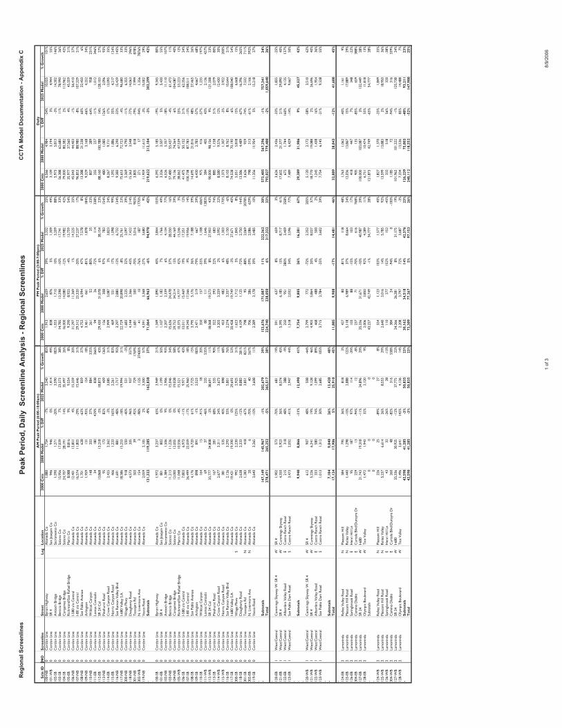
Reg
iona
l Scr
eenl
ines
Peak
Per
iod,
Dai
ly S
cree
nlin
e A
naly
sis
- Reg
iona
l Scr
eenl
ines
C
CTA
Mod
el D
ocum
enta
tion
- App
endi
x C
Scl
n ID
NO
Scr
eenl
ine
Str
eet
Leg
Lo
cati
on
2000
Cnt
s20
00 M
ode
l%
Diff
20
25 M
ode
l%
Gro
wth
2000
Cnt
s20
00 M
ode
l%
Diff
20
25 M
ode
l%
Gro
wth
2000
Cnt
s20
00 M
ode
l%
Diff
20
25 M
ode
l%
Gro
wth
100-
NB
0C
ordo
n Li
neBy
ron
Hig
hwa y
Ala
med
a C
o1,
880
1,75
4-7
%3,
240
85%
1,91
32,
659
39%
3,33
225
%6,
566
4,98
4-2
4%10
,025
101%
101-
WB
0C
ordo
n Li
neSR
4Sa
n Jo
aqui
n C
o94
694
60%
1,41
449
%83
887
65%
1,30
949
%3,
109
3,19
43%
4,94
455
%10
2-SB
0C
ordo
n Li
neA
ntio
ch B
ridg
eSa
cram
ento
Co
1,59
01,
271
-20%
3,59
018
2%1,
553
1,71
010
%3,
209
88%
5,97
35,
813
-3%
14,3
0214
6%10
3-SB
0C
ordo
n Li
neBe
nici
a Br
idge
Sola
no C
o15
,956
17,0
397%
23,5
7338
%14
,785
13,2
98-1
0%17
,741
33%
56,3
8862
,680
11%
78,9
9026
%10
4-SB
0C
ordo
n Li
neC
arqu
inez
Bri
dge
Sola
no C
o24
,707
28,1
9114
%35
,497
26%
16,0
0014
,080
-12%
19,9
8242
%79
,000
80,3
822%
113,
962
42%
105-
EB0
Cor
don
Line
Ric
hmon
d/Sa
n R
afae
l Bri
dge
Mar
in C
o8,
088
8,81
69%
9,55
48%
9,29
08,
925
-4%
13,7
5954
%35
,977
37,5
604%
45,5
5921
%10
6-N
B0
Cor
don
Line
I-580
s/o
Cen
tral
Ala
med
a C
o12
,401
12,8
514%
15,3
5920
%11
,297
11,3
691%
14,2
2525
%45
,043
44,4
03-1
%56
,410
27%
107-
NB
0C
ordo
n Li
neI-8
0 s/
o C
entr
alA
lam
eda
Co
16,5
7411
,803
-29%
15,4
4631
%29
,312
23,3
20-2
0%27
,237
17%
96,8
5388
,980
-8%
107,
329
21%
108-
NB
0C
ordo
n Li
neSa
n Pa
blo
Ave
nue
Ala
med
a C
o1,
701
628
-63%
859
37%
4,75
26,
994
47%
7,57
88%
13,2
8821
,238
60%
22,4
506%
109-
NB
0C
ordo
n Li
neA
rlin
gton
Ala
med
a C
o1,
959
131
-93%
154
18%
3,46
166
1-8
1%1,
878
184%
9,32
93,
168
-66%
4,25
234
%11
0-N
B0
Cor
don
Line
Wild
cat
Can
yon
Ala
med
a C
o14
820
337
%88
433
5%26
152
-80%
35-3
3%80
728
9-6
4%95
823
1%11
1-EB
0C
ordo
n Li
neLo
mas
Con
tadi
sA
lam
eda
Co
3418
042
9%83
836
6%94
26-7
2%11
433
8%25
522
7-1
1%1,
012
346%
112-
EB0
Cor
don
Line
SR 2
4 C
alA
lam
eda
Co
13,8
6813
,218
-5%
18,8
7343
%29
,430
31,0
786%
38,1
5423
%88
,160
100,
788
14%
128,
103
27%
113-
NB
0C
ordo
n Li
nePi
nehu
rst
Roa
dA
lam
eda
Co
9517
382
%40
913
6%15
630
897
%78
315
4%48
01,
085
126%
2,09
693
%11
4-EB
0C
ordo
n Li
neC
row
Can
yon
Roa
dA
lam
eda
Co
2,42
52,
362
-3%
3,08
531
%2,
999
3,08
73%
3,82
324
%8,
267
9,71
117
%13
,095
35%
115-
EB0
Cor
don
Line
Nor
ris
Can
yon
Roa
dA
lam
eda
Co
466
1,23
316
5%2,
261
83%
469
551
17%
1,09
899
%1,
392
1,88
635
%4,
217
124%
116-
NB
0C
ordo
n Li
neSa
n R
amon
Val
ley
Blvd
Ala
med
a C
o1,
691
881
-48%
1,71
795
%3,
297
2,88
0-1
3%6,
732
134%
9,38
36,
290
-33%
15,4
2914
5%11
7-N
B0
Cor
don
Line
I-680
Val
ley
S.A
.A
lam
eda
Co
18,5
8615
,253
-18%
19,9
9431
%22
,729
20,8
98-8
%25
,761
23%
75,6
5372
,723
-4%
96,6
8033
%30
0-N
B0
Cor
don
Line
Vill
age
Pkw
yA
lam
eda
Co
918
550
-40%
531
-3%
1,68
32,
225
32%
3,09
739
%5,
369
4,79
0-1
1%6,
355
33%
118-
NB
0C
ordo
n Li
neD
ough
erty
Roa
dA
lam
eda
Co
4,57
320
5-9
6%93
735
7%4,
144
2,36
6-4
3%7,
422
214%
15,3
633,
548
-77%
14,0
6329
6%30
1-N
B0
Cor
don
Line
Tas
saja
ra R
dA
lam
eda
Co
503
39-9
2%72
917
69%
1,68
150
0-7
0%5,
016
903%
3,80
581
8-7
9%7,
999
878%
302-
WB
0C
ordo
n Li
neN
. Liv
erm
ore
Av e
Ala
med
a C
o15
43
-98%
1,12
537
400%
4110
-76%
187
1770
%27
117
-94%
1,35
678
76%
119-
NB
0C
ordo
n Li
neV
asco
Roa
dA
lam
eda
Co
2,05
92,
105
2%3,
300
57%
4,59
13,
368
-27%
3,68
09%
11,9
5911
,613
-3%
15,0
0229
%-
Sub
tota
ls13
1,32
211
9,28
5-9
%16
2,83
837
%71
,064
66,9
63-6
%94
,970
42%
219,
622
212,
184
-3%
302,
299
42%
- 100-
SB0
Cor
don
Line
Byro
n H
ighw
a yA
lam
eda
Co
1,97
23,
257
65%
3,94
921
%1,
349
1,89
040
%3,
844
103%
6,39
25,
185
-19%
9,34
580
%10
1-EB
0C
ordo
n Li
neSR
4Sa
n Jo
aqui
n C
o80
180
20%
1,19
950
%1,
107
1,18
27%
1,76
649
%3,
326
3,50
75%
5,43
055
%10
2-N
B0
Cor
don
Line
Ant
ioch
Bri
dge
Sacr
amen
to C
o1,
384
1,50
69%
2,90
693
%2,
207
2,33
96%
4,13
477
%6,
526
5,35
7-1
8%11
,110
107%
103-
NB
0C
ordo
n Li
neBe
nici
a Br
idge
Sola
no C
o11
,213
11,2
260%
15,0
4634
%15
,636
24,4
7857
%28
,350
16%
57,4
8055
,437
-4%
61,4
7311
%10
4-N
B0
Cor
don
Line
Car
quin
ez B
ridg
eSo
lano
Co
12,0
0012
,055
0%19
,028
58%
29,7
5234
,214
15%
44,1
6929
%79
,136
74,2
64-6
%10
4,08
740
%10
5-W
B0
Cor
don
Line
Ric
hmon
d/Sa
n R
afae
l Bri
dge
Mar
in C
o11
,048
10,5
56-4
%15
,521
47%
10,3
7514
,777
42%
15,2
463%
38,0
6247
,539
25%
53,2
2312
%10
6-SB
0C
ordo
n Li
neI-5
80 s
/o C
entr
alA
lam
eda
Co
7,80
36,
973
-11%
9,97
143
%13
,011
15,4
6919
%17
,351
12%
41,4
7550
,152
21%
62,3
5624
%10
7-SB
0C
ordo
n Li
neI-8
0 s/
o C
entr
alA
lam
eda
Co
26,4
9922
,059
-17%
25,9
6018
%19
,240
17,5
66-9
%19
,956
14%
100,
738
87,7
83-1
3%10
8,51
124
%10
8-SB
0C
ordo
n Li
neSa
n Pa
blo
Ave
nue
Ala
med
a C
o4,
176
6,72
061
%7,
725
15%
3,79
55,
176
36%
7,18
839
%14
,695
21,8
1648
%27
,465
26%
109-
SB0
Cor
don
Line
Arl
ingt
onA
lam
eda
Co
898
891
-1%
2,52
318
3%2,
471
519
-79%
667
29%
6,43
02,
783
-57%
4,66
768
%11
0-SB
0C
ordo
n Li
neW
ildca
t C
anyo
nA
lam
eda
Co
164
15-9
1%18
20%
350
157
-55%
1,10
860
6%97
541
6-5
7%1,
235
197%
111-
WB
0C
ordo
n Li
neLo
mas
Con
tadi
sA
lam
eda
Co
6937
-46%
235
535%
8011
139
%1,
646
1383
%28
440
543
%2,
136
427%
112-
WB
0C
ordo
n Li
neSR
24
Cal
Ala
med
a C
o35
,777
34,8
08-3
%38
,691
11%
18,0
6819
,573
8%27
,903
43%
90,0
0098
,156
9%12
1,20
823
%11
3-SB
0C
ordo
n Li
nePi
nehu
rst
Roa
dA
lam
eda
Co
167
281
68%
535
90%
322
393
22%
683
74%
885
1,15
831
%2,
079
80%
114-
WB
0C
ordo
n Li
neC
row
Can
yon
Roa
dA
lam
eda
Co
2,67
73,
311
24%
3,67
311
%3,
203
3,25
92%
3,99
222
%8,
580
9,57
612
%12
,430
30%
115-
WB
0C
ordo
n Li
neN
orri
s C
anyo
n R
oad
Ala
med
a C
o38
153
540
%89
868
%45
348
26%
1,30
317
0%1,
373
1,30
7-5
%3,
922
200%
116-
SB0
Cor
don
Line
San
Ram
on V
alle
y Bl
vdA
lam
eda
Co
2,12
63,
293
55%
5,80
176
%2,
274
3,35
748
%3,
150
-6%
8,10
38,
762
8%10
,644
21%
117-
SB0
Cor
don
Line
I-680
Val
ley
S.A
.A
lam
eda
Co
19,4
2119
,390
0%29
,693
53%
20,4
5819
,749
-3%
27,6
7140
%74
,528
70,1
90-6
%10
8,04
054
%30
0-SB
0C
ordo
n Li
neV
illag
e Pk
wy
SA
lam
eda
Co
992
2,23
012
5%2,
925
31%
1,62
31,
712
5%1,
845
8%5,
051
5,81
815
%6,
668
15%
118-
SB0
Cor
don
Line
Dou
gher
ty R
oad
Ala
med
a C
o2,
638
2,33
3-1
2%8,
883
281%
4,10
91,
125
-73%
2,75
014
4%13
,586
4,48
9-6
7%16
,396
265%
301-
SB0
Cor
don
Line
Tas
saja
ra R
dN
Ala
med
a C
o1,
283
418
-67%
3,85
182
1%79
895
-88%
2,06
920
78%
3,62
692
9-7
4%7,
532
711%
302-
EB0
Cor
don
Line
N. L
iver
mor
e A
v eN
Ala
med
a C
o20
6-7
0%40
567%
706
286
-59%
2,08
662
9%79
831
3-6
1%2,
166
592%
119-
SB0
Cor
don
Line
Vas
co R
oad
Ala
med
a C
o3,
640
3,26
5-1
0%3,
608
11%
2,28
93,
178
39%
3,48
510
%11
,356
11,9
545%
15,2
1827
%- -
Sub
tota
ls14
7,14
914
5,96
7-1
%20
2,67
939
%15
3,67
617
1,08
711
%22
2,36
230
%57
3,40
556
7,29
6-1
%75
7,34
134
%T
ota
l27
8,47
126
5,25
2-5
%36
5,51
738
%22
4,74
023
8,05
06%
317,
332
33%
793,
027
779,
480
-2%
1,05
9,64
036
%- 12
0-EB
1W
est/
Cen
tral
Cum
min
gs S
kyw
ay W
. SR
4W
SR 4
1,90
257
3-7
0%68
119
%59
163
78%
659
3%3,
626
2,43
6-3
3%1,
835
-25%
121-
EB1
Wes
t/C
entr
alSR
4W
Cum
min
gs S
kyw
ay4,
350
5,92
336
%8,
574
45%
5,39
56,
185
15%
8,71
741
%17
,602
21,3
7721
%29
,890
40%
122-
EB1
Wes
t/C
entr
alA
lham
bra
Val
ley
Roa
dE
Cas
tro
Ran
ch R
oad
215
318
48%
288
-9%
250
951
280%
3,40
925
8%67
21,
744
160%
4,13
513
7%12
3-EB
1W
est/
Cen
tral
San
Pabl
o D
am R
oad
SC
astr
o R
anch
Roa
d3,
473
2,05
2-4
1%2,
947
44%
1,51
82,
032
34%
3,59
677
%7,
489
6,42
9-1
4%9,
667
50%
- -S
ubto
tals
9,94
08,
866
-11%
12,4
9041
%7,
754
9,80
526
%16
,381
67%
29,3
8931
,986
9%45
,527
42%
- 120-
WB
1W
est/
Cen
tral
Cum
min
gs S
kyw
ay W
. SR
4W
SR 4
612
907
48%
508
-44%
2,79
977
2-7
2%2,
352
205%
5,12
02,
172
-58%
3,51
062
%12
1-W
B1
Wes
t/C
entr
alSR
4W
Cum
min
gs S
kyw
ay5,
226
6,24
119
%9,
128
46%
4,90
35,
864
20%
8,02
737
%18
,770
19,0
882%
26,6
9640
%12
2-W
B1
Wes
t/C
entr
alA
lham
bra
Val
ley
Roa
dE
Cas
tro
Ran
ch R
oad
333
580
74%
1,09
989
%46
848
84%
500
2%1,
245
1,43
816
%1,
954
36%
123-
WB
1W
est/
Cen
tral
San
Pabl
o D
am R
oad
SC
astr
o R
anch
Roa
d1,
013
1,31
230
%2,
685
105%
3,71
52,
784
-25%
3,60
229
%7,
754
6,14
5-2
1%9,
528
55%
- -S
ubto
tals
7,18
49,
040
26%
13,4
2048
%T
ota
l17
,124
17,9
065%
25,9
1045
%11
,885
9,90
8-1
7%14
,481
46%
32,8
8928
,843
-12%
41,6
8845
%- 12
4-EB
2La
mor
ind a
Rel
iez
Val
ley
Roa
dN
Plea
sant
Hill
584
795
36%
818
3%42
780
-81%
118
48%
1,76
31,
062
-40%
1,16
19%
125-
EB2
Lam
orin
d aPl
easa
nt H
ill R
oad
NR
elie
z V
alle
y1,
440
1,29
8-1
0%2,
888
122%
5,11
86,
989
37%
8,66
424
%12
,036
13,8
6715
%17
,889
29%
126-
EB2
Lam
orin
d aSp
ring
broo
k R
oad
EH
enri
Hill
Ln
9518
797
%11
4-3
9%10
388
-15%
103
17%
418
447
7%34
8-2
2%30
4-EB
2La
mor
ind a
Cam
ino
Dia
blo
EC
urto
la B
lvd/
Dun
syre
Dr
229
13-9
4%12
-8%
237
71-7
0%61
676
8%90
513
5-8
5%65
938
8%12
7-EB
2La
mor
ind a
SR 2
4W
I-680
21
,743
19,3
18-1
1%24
,896
29%
35,3
3631
,671
-10%
40,9
8729
%10
0,00
010
3,08
73%
132,
449
28%
128-
EB2
Lam
orin
d aO
lym
pic
Boul
evar
dW
Tic
e V
alle
y1,
472
1,94
332
%2,
120
9%2,
006
3,85
092
%4,
289
11%
6,75
110
,474
55%
11,8
1813
%-
Subt
otal
s0
00
43,2
2742
,749
-1%
54,7
7728
%12
1,87
342
,749
-65%
54,7
7728
%-
00
012
4-W
B2
Lam
orin
d aR
elie
z V
alle
y R
oad
NPl
easa
nt H
ill22
625
-89%
278%
554
1,12
310
3%1,
577
40%
1,82
71,
370
-25%
1,84
935
%12
5-W
B2
Lam
orin
d aPl
easa
nt H
ill R
oad
NR
elie
z V
alle
y5,
237
6,61
426
%8,
553
29%
2,64
03,
016
14%
5,78
592
%13
,599
13,8
832%
18,9
5036
%12
6-W
B2
Lam
orin
d aSp
ring
broo
k R
oad
EH
enri
Hill
Ln
4332
-26%
28-1
3%11
027
715
2%15
2-4
5%33
251
856
%32
0-3
8%30
4-W
B2
Lam
orin
d aC
amin
o D
iabl
oE
Cur
tola
Blv
d/D
unsy
re D
r26
048
-82%
316
558%
384
24-9
4%0
-100
%1,
185
72-9
4%31
633
9%12
7-W
B2
Lam
orin
d aSR
24
WI-6
80
35,3
3630
,925
-12%
37,7
7522
%24
,266
26,2
818%
31,1
7519
%10
1,96
210
1,22
2-1
%12
5,73
824
%12
8-W
B2
Lam
orin
d aO
lym
pic
Boul
evar
dW
Tic
e V
alle
y1,
496
3,64
114
3%4,
136
14%
2,20
83,
797
72%
3,68
7-3
%7,
334
13,5
3685
%14
,488
7%-
Sub
tota
ls42
,598
41,2
85-3
%50
,835
23%
30,1
6234
,518
14%
42,3
7623
%12
6,23
975
,803
-40%
93,2
1123
%T
ota
l42
,598
41,2
85-3
%50
,835
23%
73,3
8977
,267
5%97
,153
26%
248,
112
118,
552
-52%
147,
988
25%
Dai
ly
AM
Pea
k P
erio
d (6
:00-
10:0
0am
)P
M P
eak
Per
iod
(3:0
0-7:
00pm
)
1 of
38/
9/20
06

Reg
iona
l Scr
eenl
ines
Peak
Per
iod,
Dai
ly S
cree
nlin
e A
naly
sis
- Reg
iona
l Scr
eenl
ines
C
CTA
Mod
el D
ocum
enta
tion
- App
endi
x C
Scl
n ID
NO
Scr
eenl
ine
Str
eet
Leg
Lo
cati
on
2000
Cnt
s20
00 M
ode
l%
Diff
20
25 M
ode
l%
Gro
wth
2000
Cnt
s20
00 M
ode
l%
Diff
20
25 M
ode
l%
Gro
wth
2000
Cnt
s20
00 M
ode
l%
Diff
20
25 M
ode
l%
Gro
wth
Dai
ly
AM
Pea
k P
erio
d (6
:00-
10:0
0am
)P
M P
eak
Per
iod
(3:0
0-7:
00pm
)
- 129-
NB
3T
ri-V
alle
yD
anvi
lle B
oule
vard
NLi
vorn
a 78
989
513
%4,
087
357%
2,03
33,
777
86%
4,36
416
%5,
148
4,92
6-4
%10
,230
108%
130-
NB
3T
ri-V
alle
yI-6
80N
Livo
rna
24,2
3226
,693
10%
37,9
2442
%29
,271
30,7
535%
30,3
01-1
%10
5,56
010
4,59
1-1
%11
6,72
012
%30
5-N
B3
Tri
-Val
ley
Tro
tter
Way
NLi
vorn
a 18
632
-83%
793
2378
%57
737
4-3
5%1,
829
389%
1,67
541
0-7
6%2,
632
542%
306-
NB
3T
ri-V
alle
yLa
vend
er D
rN
Livo
rna
145
47-6
8%19
030
4%37
246
926
%2,
026
332%
1,04
299
1-5
%2,
673
170%
-S
ubto
tals
25,3
5227
,667
9%42
,994
55%
32,2
5335
,373
10%
38,5
209%
113,
425
110,
918
-2%
132,
255
19%
- 129-
SB3
Tri
-Val
ley
Dan
ville
Bou
leva
rdN
Livo
rna
2,02
01,
921
-5%
4,24
512
1%2,
114
2,25
16%
4,26
089
%6,
376
4,33
7-3
2%9,
668
123%
130-
SB3
Tri
-Val
ley
I-680
NLi
vorn
a 25
,001
28,6
1014
%30
,010
5%29
,001
31,5
959%
31,0
48-2
%10
0,00
110
6,36
36%
113,
450
7%30
5-SB
3T
ri-V
alle
yT
rott
er W
ayN
Livo
rna
519
169
-67%
1,64
287
2%40
810
3-7
5%1,
835
1682
%1,
664
286
-83%
3,49
211
21%
306-
SB3
Tri
-Val
ley
Lave
nder
Dr
NLi
vorn
a 38
426
1-3
2%1,
049
302%
278
156
-44%
1,48
685
3%1,
157
712
-38%
2,89
230
6%-
Sub
tota
ls27
,924
30,9
6111
%36
,946
19%
31,8
0134
,105
7%38
,629
13%
109,
198
111,
698
2%12
9,50
216
%T
ota
l53
,276
58,6
2810
%79
,940
36%
64,0
5469
,478
8%77
,149
11%
222,
623
222,
616
0%26
1,75
718
%- 13
2-EB
4C
entr
al/E
ast
SR 4
EPo
rt C
hica
g o9,
821
11,2
4014
%14
,934
33%
24,8
7529
,991
21%
40,2
6734
%72
,962
85,4
7417
%11
0,94
530
%30
7-EB
4C
entr
al/E
ast
Will
ow P
ass
Rd
NLy
nwoo
d D
r2,
283
1,56
2-3
2%3,
447
121%
3,66
03,
109
-15%
3,83
823
%11
,281
6,43
2-4
3%9,
541
48%
133-
EB4
Cen
tral
/Eas
tBa
iley
Roa
dE
Myr
tle61
11,
049
72%
1,38
132
%2,
128
1,52
2-2
8%3,
965
161%
4,51
24,
050
-10%
8,20
110
2%13
5-EB
4C
entr
al/E
ast
Kir
ker
Pass
Roa
dE
Myr
tle1,
622
1,50
1-7
%2,
523
68%
7,19
86,
167
-14%
7,89
628
%13
,880
10,9
46-2
1%15
,069
38%
136-
EB4
Cen
tral
/Eas
tM
arsh
Cre
ek R
oad
EC
layt
on54
325
7-5
3%28
210
%2,
608
1,96
7-2
5%4,
051
106%
5,33
33,
230
-39%
5,82
580
%- -
Sub
tota
ls14
,880
15,6
095%
22,5
6745
%40
,469
42,7
566%
60,0
1740
%10
7,96
811
0,13
22%
149,
581
36%
- 132-
WB
4C
entr
al/E
ast
SR 4
EPo
rt C
hica
g o25
,240
29,0
9315
%39
,665
36%
13,6
5717
,448
28%
21,7
6725
%74
,973
79,7
086%
104,
111
31%
307-
WB
4C
entr
al/E
ast
Will
ow P
ass
Rd
NLy
nwoo
d D
r3,
147
2,62
6-1
7%3,
786
44%
2,92
01,
273
-56%
2,52
899
%10
,810
5,42
1-5
0%8,
245
52%
133-
WB
4C
entr
al/E
ast
Baile
y R
oad
EM
yrtle
1,62
82,
154
32%
4,06
789
%85
91,
175
37%
2,06
476
%3,
958
4,87
923
%8,
852
81%
135-
WB
4C
entr
al/E
ast
Kir
ker
Pass
Roa
dE
Myr
tle5,
636
6,44
814
%7,
789
21%
1,83
52,
418
32%
3,91
162
%11
,814
11,7
650%
16,0
6037
%13
6-W
B4
Cen
tral
/Eas
tM
arsh
Cre
ek R
oad
EC
layt
on2,
475
1,53
0-3
8%3,
997
161%
860
546
-37%
707
29%
5,23
02,
977
-43%
5,98
410
1%- -
Sub
tota
ls38
,126
41,8
5110
%59
,304
42%
20,1
3122
,860
14%
30,9
7736
%10
6,78
510
4,75
0-2
%14
3,25
237
%T
ota
l53
,006
57,4
608%
81,8
7142
%60
,600
65,6
168%
90,9
9439
%21
4,75
321
4,88
20%
292,
833
36%
- 137-
EB5
S.C
Cen
tral
Tre
at B
oule
vard
WO
ak G
rove
2,72
21,
116
-59%
2,07
486
%7,
458
6,43
4-1
4%10
,331
61%
19,8
5711
,528
-42%
17,4
4051
%13
8-EB
5S.
C C
entr
alY
gnac
io V
alle
y R
oad
WO
ak G
rove
2,90
31,
979
-32%
2,67
835
%9,
506
11,9
1325
%12
,644
6%23
,807
23,7
890%
27,1
0514
%-
Sub
tota
ls5,
625
3,09
5-4
5%4,
752
54%
16,9
6418
,347
8%22
,975
25%
43,6
6435
,317
-19%
44,5
4526
%- 13
7-W
B5
S.C
Cen
tral
Tre
at B
oule
vard
WO
ak G
rove
6,91
47,
955
15%
10,3
5730
%3,
958
2,37
4-4
0%3,
433
45%
19,8
4814
,144
-29%
18,1
0928
%13
8-W
B5
S.C
Cen
tral
Ygn
acio
Val
ley
Roa
dW
Oak
Gro
ve7,
509
11,1
6149
%11
,850
6%4,
258
4,17
2-2
%5,
716
37%
21,8
6223
,585
8%27
,589
17%
-S
ubto
tals
14,4
2319
,116
33%
22,2
0716
%8,
216
6,54
6-2
0%9,
149
40%
41,7
1037
,729
-10%
45,6
9821
%T
ota
l20
,048
22,2
1111
%26
,959
21%
25,1
8024
,893
-1%
32,1
2429
%85
,374
73,0
46-1
4%90
,243
24%
- 140-
EB6
S.C
Eas
tBu
chan
an
Roa
dW
Can
al1,
307
942
-28%
3,41
226
2%4,
988
3,58
0-2
8%3,
294
-8%
10,4
648,
224
-21%
12,4
2251
%30
3-EB
6S.
C E
ast
Del
ta F
air
Blvd
EK
endr
ee S
t73
239
1-4
7%47
321
%3,
852
6,12
459
%5,
578
-9%
8,37
28,
607
3%7,
164
-17%
141-
EB6
S.C
Eas
tSR
4W
Som
ersv
ille
8,23
810
,428
27%
12,9
7324
%17
,724
19,7
5311
%22
,057
12%
56,9
6757
,950
2%66
,940
16%
308-
EB6
S.C
Eas
tC
entu
ry B
lvd
WLo
s M
edan
os W
ater
way
350
81-7
7%77
-5%
1,74
72,
377
36%
1,42
6-4
0%4,
214
3,38
6-2
0%1,
759
-48%
142-
EB6
S.C
Eas
tPi
ttsb
urg/
Ant
ioch
Hig
hway
WV
ern
Rob
erts
Cir
cle
559
447
-20%
296
-34%
3,55
73,
929
10%
6,56
967
%5,
977
7,80
331
%7,
501
-4%
- -S
ubto
tals
11,1
8612
,289
10%
17,2
3140
%31
,868
35,7
6312
%38
,924
9%85
,994
85,9
700%
95,7
8611
%- 14
0-W
B6
S.C
Eas
tBu
chan
an
Roa
dW
Can
al3,
785
3,57
7-5
%3,
275
-8%
2,01
52,
964
47%
3,71
525
%9,
772
9,88
51%
9,74
3-1
%30
3-W
B6
S.C
Eas
tD
elta
Fai
r Bl
vdE
Ken
dree
St
3,05
83,
923
28%
4,40
112
%1,
783
917
-49%
939
2%8,
065
6,00
6-2
6%6,
539
9%14
1-W
B6
S.C
Eas
tSR
4W
Som
ersv
ille
16,1
9719
,646
21%
22,8
8116
%13
,140
13,1
870%
17,5
1533
%60
,705
57,8
21-5
%67
,541
17%
308-
WB
6S.
C E
ast
Cen
tury
Blv
dW
Los
Med
anos
Wat
erw
ay1,
811
2,22
123
%93
6-5
8%1,
063
554
-48%
412
-26%
5,18
53,
597
-31%
1,60
6-5
5%14
2-W
B6
S.C
Eas
tPi
ttsb
urg/
Ant
ioch
Hig
hway
WV
ern
Rob
erts
Cir
cle
3,70
93,
804
3%4,
215
11%
1,78
31,
032
-42%
553
-46%
9,40
85,
759
-39%
5,39
1-6
%- -
Sub
tota
ls28
,560
33,1
7116
%35
,708
8%19
,784
18,6
54-6
%23
,134
24%
93,1
3583
,068
-11%
90,8
209%
To
tal
39,7
4645
,460
14%
52,9
3916
%51
,652
54,4
175%
62,0
5814
%17
9,12
916
9,03
8-6
%18
6,60
610
%- 14
3-N
B7
S.C
Tri
-Val
ley
I-680
SSy
cam
ore
Val
ley
19,4
3117
,828
-8%
22,2
2025
%28
,221
26,6
05-6
%29
,006
9%87
,886
88,2
320%
98,7
0812
%14
4-N
B7
S.C
Tri
-Val
ley
San
Ram
on B
oule
vard
SSy
cam
ore
Val
ley
1,56
156
6-6
4%1,
194
111%
3,55
43,
217
-9%
3,15
7-2
%9,
152
5,39
6-4
1%6,
754
25%
- -S
ubto
tals
20,9
9218
,394
-12%
23,4
1427
%31
,775
29,8
22-6
%32
,163
8%97
,038
93,6
28-4
%10
5,46
213
%- 14
3-SB
7S.
C T
ri-V
alle
yI-6
80S
Syca
mor
e V
alle
y22
,090
25,5
8316
%28
,712
12%
20,4
5924
,444
19%
28,1
1515
%86
,001
88,5
743%
102,
041
15%
144-
SB7
S.C
Tri
-Val
ley
San
Ram
on B
oulv
ard
SSy
cam
ore
Val
ley
1,79
53,
523
96%
3,65
24%
2,49
01,
770
-29%
2,84
661
%8,
490
7,41
1-1
3%9,
119
23%
- -S
ubto
tals
23,8
8529
,106
22%
32,3
6411
%22
,949
26,2
1414
%30
,961
18%
94,4
9195
,985
2%11
1,16
016
%T
ota
l44
,877
47,5
006%
55,7
7817
%54
,724
56,0
362%
63,1
2413
%19
1,52
918
9,61
3-1
%21
6,62
214
%
2 of
38/
9/20
06

Reg
iona
l Scr
eenl
ines
Peak
Per
iod,
Dai
ly S
cree
nlin
e A
naly
sis
- Reg
iona
l Scr
eenl
ines
C
CTA
Mod
el D
ocum
enta
tion
- App
endi
x C
Scl
n ID
NO
Scr
eenl
ine
Str
eet
Leg
Lo
cati
on
2000
Cnt
s20
00 M
ode
l%
Diff
20
25 M
ode
l%
Gro
wth
2000
Cnt
s20
00 M
ode
l%
Diff
20
25 M
ode
l%
Gro
wth
2000
Cnt
s20
00 M
ode
l%
Diff
20
25 M
ode
l%
Gro
wth
Dai
ly
AM
Pea
k P
erio
d (6
:00-
10:0
0am
)P
M P
eak
Per
iod
(3:0
0-7:
00pm
)
- 145-
NB
8S.
C W
est
I-80
SSR
416
,642
15,8
04-5
%22
,760
44%
35,1
4837
,480
7%46
,896
25%
86,0
0197
,780
14%
132,
728
36%
146-
NB
8S.
C W
est
San
Pabl
o A
venu
eN
Pino
le V
alle
y1,
326
810
-39%
2,47
920
6%4,
470
7,07
158
%8,
414
19%
10,7
749,
354
-13%
13,7
8547
%- -
Sub
tota
ls17
,968
16,6
14-8
%25
,239
52%
39,6
1844
,551
12%
55,3
1024
%96
,775
107,
134
11%
146,
513
37%
- 145-
SB8
S.C
Wes
tI-8
0S
SR 4
29,9
3435
,825
20%
44,7
4825
%20
,026
19,5
70-2
%24
,218
24%
86,0
4410
3,25
420
%14
0,96
337
%14
6-SB
8S.
C W
est
San
Pabl
o A
venu
eN
Pino
le V
alle
y3,
245
4,85
149
%7,
918
63%
2,12
21,
124
-47%
4,98
034
3%9,
374
7,56
3-1
9%16
,160
114%
- -S
ubto
tals
33,1
7940
,676
23%
52,6
6629
%22
,148
20,6
94-7
%29
,198
41%
95,4
1811
0,81
716
%15
7,12
342
%T
ota
l51
,147
57,2
9012
%77
,905
36%
61,7
6665
,245
6%84
,508
30%
192,
193
217,
951
13%
303,
636
39%
- 279-
EB9
Ala
med
a C
ount
yC
row
Can
yon
WC
ount
y Li
ne2,
425
2,34
3-3
%2,
132
-9%
2,99
93,
080
3%3,
266
6%8,
267
9,66
717
%10
,625
10%
280-
EB9
Ala
med
a C
ount
yN
orri
s C
anyo
n W
Cou
nty
Line
473
1,23
316
1%2,
261
83%
478
551
15%
1,09
899
%1,
425
1,88
632
%4,
217
124%
281-
EB9
Ala
med
a C
ount
yI-5
80
WC
ount
y Li
ne33
,669
29,8
52-1
1%37
,363
25%
27,3
2929
,957
10%
38,5
5529
%11
8,24
810
5,13
5-1
1%14
5,56
638
%28
2-EB
9A
lam
eda
Cou
nty
Dub
lin C
anyo
n W
Cou
nty
Line
983
382
-61%
482
26%
1,28
661
5-5
2%69
813
%3,
399
1,84
3-4
6%2,
176
18%
- -S
ubto
tals
37,5
5033
,810
-10%
42,2
3825
%32
,092
34,2
037%
43,6
1728
%13
1,33
911
8,53
1-1
0%16
2,58
437
%- 27
9-W
B9
Ala
med
a C
ount
yC
row
Can
yon
WC
ount
y Li
ne2,
677
3,31
224
%3,
465
5%3,
203
3,23
71%
2,86
1-1
2%8,
580
9,53
411
%9,
995
5%28
0-W
B9
Ala
med
a C
ount
yN
orri
s C
anyo
n W
Cou
nty
Line
392
535
36%
898
68%
469
482
3%1,
303
170%
1,43
41,
307
-9%
3,92
220
0%28
1-W
B9
Ala
med
a C
ount
yI-5
80
WC
ount
y Li
ne30
,521
30,8
601%
37,5
0822
%31
,162
26,3
18-1
6%34
,621
32%
119,
363
107,
015
-10%
149,
845
40%
282-
WB
9A
lam
eda
Cou
nty
Dub
lin C
anyo
n W
Cou
nty
Line
2,20
355
7-7
5%62
612
%92
353
6-4
2%66
123
%4,
248
1,85
8-5
6%2,
208
19%
- -S
ubto
tals
35,7
9335
,264
-1%
42,4
9721
%35
,757
30,5
73-1
4%39
,446
29%
133,
625
119,
714
-10%
165,
970
39%
To
tal
73,3
4369
,074
-6%
84,7
3523
%67
,849
64,7
76-5
%83
,063
28%
264,
964
238,
245
-10%
328,
554
38%
- 287-
NB
10Su
nol
I-680
N
Rte
84
11,9
1211
,789
-1%
16,6
1441
%19
,952
22,9
3115
%25
,856
13%
61,1
0371
,099
16%
88,1
6124
%28
8-N
B10
Suno
lSR
84
EI-6
80
1,53
41,
164
-24%
6,23
543
6%5,
935
3,94
4-3
4%13
,253
236%
14,1
459,
377
-34%
37,9
4030
5%- -
Sub
tota
ls13
,446
12,9
53-4
%22
,849
76%
25,8
8726
,875
4%39
,109
46%
75,2
4880
,476
7%12
6,10
157
%- 28
7-SB
10Su
nol
I-680
N
Rte
84
15,5
2816
,881
9%21
,629
28%
14,8
4516
,933
14%
20,0
8619
%61
,181
69,5
6414
%86
,335
24%
288-
SB10
Suno
lSR
84
EI-6
80
3,61
03,
722
3%12
,240
229%
1,79
42,
954
65%
7,65
315
9%11
,082
14,1
4128
%45
,299
220%
- -S
ubto
tals
19,1
3820
,603
8%33
,869
64%
16,6
3919
,887
20%
27,7
3939
%72
,263
83,7
0516
%13
1,63
457
%T
ota
l32
,584
33,5
563%
56,7
1869
%42
,526
46,7
6210
%66
,848
43%
147,
511
164,
181
11%
257,
735
57%
- 283-
EB11
Gre
envi
lle R
oad
Alta
mon
t Pa
ss
EG
reen
ville
457
558
22%
813
46%
2,98
33,
139
5%4,
192
34%
4,64
44,
067
-12%
6,08
950
%28
4-EB
11G
reen
ville
Roa
dI-5
80E
Gre
envi
lle8,
438
10,3
5223
%16
,686
61%
23,5
2024
,541
4%38
,273
56%
62,2
8065
,619
5%12
2,46
387
%28
5-EB
11G
reen
ville
Roa
dPa
tter
son
Pass
E
Gre
envi
lle96
960%
154
60%
924
929
1%1,
504
62%
1,27
11,
283
1%2,
230
74%
286-
EB11
Gre
envi
lle R
oad
Tes
la R
oad
EG
reen
ville
234
235
0%37
961
%1,
857
1,86
71%
3,02
262
%2,
927
2,96
61%
5,31
979
%- -
Sub
tota
ls9,
225
11,2
4122
%18
,032
60%
29,2
8430
,476
4%46
,991
54%
71,1
2273
,935
4%13
6,10
184
%- 28
3-W
B11
Gre
envi
lle R
oad
Alta
mon
t Pa
ss
EG
reen
ville
3,33
03,
036
-9%
3,39
912
%24
828
917
%50
575
%5,
422
5,17
7-5
%6,
725
30%
284-
WB
11G
reen
ville
Roa
dI-5
80E
Gre
envi
lle19
,455
19,5
841%
31,0
5259
%10
,163
9,95
8-2
%15
,778
58%
61,0
0264
,374
6%12
2,35
190
%28
5-W
B11
Gre
envi
lle R
oad
Patt
erso
n Pa
ss
EG
reen
ville
1,08
91,
089
0%1,
762
62%
7680
5%12
961
%1,
473
1,49
72%
2,61
875
%28
6-W
B11
Gre
envi
lle R
oad
Tes
la R
oad
EG
reen
ville
1,87
71,
877
0%3,
039
62%
2,18
62,
186
0%3,
539
62%
5,71
75,
838
2%10
,519
80%
Sub
tota
ls25
,751
25,5
86-1
%39
,252
53%
12,6
7312
,513
-1%
19,9
5159
%73
,614
76,8
864%
142,
213
85%
To
tal
34,9
7636
,827
5%57
,284
56%
41,9
5742
,989
2%66
,942
56%
144,
736
150,
821
4%27
8,31
485
%
Gra
nd T
ota
l74
1,19
675
2,44
92%
1,01
6,39
135
%77
6,19
181
5,33
45%
1,05
7,67
630
%2,
713,
340
2,57
0,41
1-5
%3,
469,
455
35%
3 of
38/
9/20
06

Appendix I - Standard Agreement Regarding Use of
the Authority’s Travel Demand Forecasting Models and Databases


CONTRA COSTA TRANSPORTATION AUTHORITY
AGREEMENT TDFM XX-XX FOR USE OF THE
CONTRA COSTA TRANSPORTATION AUTHORITY TRAVEL DEMAND FORECASTING MODEL AND GIS
CONTRA COSTA TRANSPORTATION AUTHORITY (“CCTA”) and XXXX (“USER”) as of the date set forth below, do hereby agree as follows:
1. CCTA agrees to provide USER a personal, non-transferable and non-exclusive license to use and adapt data files from its Transportation Demand Forecasting Model and Countywide GIS, or portions thereof, including all input and output files (electronic or otherwise) and any data, including but not limited to traffic count, land use, and network data, needed to run the EMME/2, TransCAD®, TP+, or ArcView or any similar software for the purpose set forth in Paragraph 2.b. below, including the West, Central, East, Tri-Valley, CMP and Countywide models, inclusively, the “MODEL.”
2. USER agrees:
a. to only install, operate and use the MODEL on a computer system owned, leased or otherwise controlled by USER in its own facilities;
b. to use and execute all portions of the MODEL on such computer systems for the limited purpose of miscellaneous traffic impact studies for new development proposals, associated environmental impact analyses, fee impact studies, transportation project analysis, and the evaluation of proposed transportation strategies and plans;
c. to only make such number of copies of the MODEL as necessary for the foregoing purposes, and a further reasonable number of copies solely for nonproductive back-up purposes in accordance with its standard procedures, provided that it accounts for such copies;
d. to use the MODEL in accordance with the most current published version of CCTA's Technical Procedures;
e. prior to using the model or data, to notify CCTA in writing of each specific study or project User expects to undertake;
f. to provide CCTA with written documentation of any revisions to the MODEL.

Agreement No. TDFM XX-XX Page 2 of 3 Month XX, 201X
3. Any use, copying, distribution, adaptation or public display of the MODEL by USER not authorized by this Agreement shall automatically terminate USER's rights hereunder. Use of the MODEL on processors accessible through communications networks through terminals and devices not on premises owned or controlled by USER is prohibited unless otherwise agreed in writing by CCTA. USER shall promptly notify CCTA and make available to it all modifications, additions, or updates USER makes to the MODEL and shall grant CCTA a perpetual, royalty-free license to use, reproduce, sublicense, and to otherwise make available to third parties the MODEL as modified, and to modify such modifications, additions, or updates.
4. Title to the MODEL, including all modifications, additions, deletions, input and output file additions and modifications, updates, copies and derivative works thereof by USER, shall be in and remain with CCTA. User hereby assigns to CCTA ownership of all such modifications, additions, deletions, input and output file additions and modifications, updates, copies and derivative works, including output from operations models (ex. FREQ, Paramics, VISSIM) which rely on MODEL data as input.
5. CCTA, ITS AFFILIATES, SUBCONTRACTORS AND REPRESENTATIVES MAKE NO WARRANTIES, EXPRESS OR IMPLIED, AND SPECIFICALLY DISCLAIM ANY WARRANTIES INCLUDING, WITHOUT LIMITATION, ANY WARRANTY OF MERCHANTABILITY OR FITNESS FOR A PARTICULAR PURPOSE OF THE MODEL. USER AGREES THAT ITS SOLE REMEDY AGAINST CCTA, ITS AFFILIATES, SUBCONTRACTORS AND REPRESENTATIVES FOR LOSS OR DAMAGE CAUSED BY ANY DEFECT OR FAILURE OF THE MODEL, REGARDLESS OF THE FORM OF ACTION, WHETHER IN CONTRACT, TORT, INCLUDING NEGLIGENCE, STRICT LIABILITY OR OTHERWISE, SHALL, TO THE EXTENT FEASIBLE (AS DETERMINED SOLELY BY CCTA) BE THE REPAIR OR REPLACEMENT OF THE MODEL. IN NO EVENT SHALL CCTA, ITS AFFILIATES, SUBCONTRACTORS OR REPRESENTATIVES BE LIABLE FOR INCIDENTAL, INDIRECT, SPECIAL OR CONSEQUENTIAL DAMAGES, OR FOR LOST PROFITS, SAVINGS, OR REVENUES OF ANY KIND, OR FOR LOST DATA OR DOWNTIME, WHETHER OR NOT CCTA, ITS AFFILIATES, SUBCONTRACTORS OR REPRESENTATIVES HAVE BEEN ADVISED OF THE POSSIBILITY OF SUCH DAMAGES.
6. This Agreement shall be effective as of the date set forth below and, unless terminated in accordance with Section 3 above or extended by written amendment to this Agreement, shall terminate on the earlier of the date that USER is not making use of the MODEL or Month XX, 201X. Upon termination, or upon immediate request by CCTA, USER shall return all copies, and submit any modifications or derivative works and accompanying documentation of revisions to

Agreement No. TDFM XX-XX Page 3 of 3 Month XX, 201X
S:\14.Planning\MODELING\Model Loan\TDFM\Agreement Templates\CCTA_TDFM_Agreement_template.docx
CCTA. Thereafter, the provisions of Sections 3, 4, 5 and 8 shall continue to apply in accordance with their terms, notwithstanding the termination of this Agreement. The medium for submittals of electronic data files to CCTA shall be arranged by USER in consultation with CCTA. Writeable CD is an acceptable medium for submittal of electronic files.
7. This Agreement shall inure to the benefit of, and shall be binding on, USER and CCTA and their respective successors and assigns, provided that USER shall not assign this Agreement or any right to use of the MODEL as provided herein, except to a successor to all or substantially all of the business and properties of USER, without the express prior written consent of CCTA.
8. This Agreement and the rights and obligations of the parties with respect to the MODEL shall be governed by California law, as it applies to a contract negotiated, executed and performed in that state.
USER ACKNOWLEDGES THAT IT HAS READ THIS AGREEMENT AND UNDERSTANDS IT, AND THAT BY ENTERING INTO THE AGREEMENT, INSTALLING AND EXECUTING THE MODEL, OR MAKING ANY OTHER USE OF IT, USER AGREES TO BE BOUND BY THE TERMS AND CONDITIONS HEREOF. THE PARTIES FURTHER AGREE THAT, EXCEPT FOR SEPARATE WRITTEN AGREEMENTS BETWEEN CCTA AND USER, THIS AGREEMENT IS THE COMPLETE AND EXCLUSIVE STATEMENT OF THE RIGHTS AND LIABILITIES OF THE PARTIES.
This Agreement is made as of Month XX, 201X.
CCTA Contra Costa Transportation Authority 2999 Oak Road, Suite 100 Walnut Creek, CA 94597
USER Agency/Consultancy Name Address City, CA 9XXXX
By:_____________________________ Martin R. Engelmann, P.E. Deputy Executive Director, Planning
By:______________________________ Agency/Consultant Designee Title