Draft Report - Welcome to the Southwest Florida Water ...
71
WEEKI WACHEE NATURAL SYSTEM CARRYING CAPACITY STUDY-ANALYSIS AND REPORTING (WW06) TASK #4 DRAFT REPORT Prepared for Southwest Florida Water Management District Tampa, FL 33637 and Hernando County Brooksville, FL 34604 Prepared by Wood Environment & Infrastructure Solutions, Inc. 1101 Channelside Drive, Suite 200 Tampa, FL 33602 Wood Project No. 600308x24 TWA NO. 19TW0002077 November 2019
Transcript of Draft Report - Welcome to the Southwest Florida Water ...

WEEKI WACHEE NATURAL SYSTEM CARRYING CAPACITY STUDY-ANALYSIS AND
REPORTING (WW06)
TASK #4
DRAFT REPORT
Prepared for
Southwest Florida Water Management District
Tampa, FL 33637
and
Hernando County
Brooksville, FL 34604
Prepared by
Wood Environment & Infrastructure Solutions, Inc.
1101 Channelside Drive, Suite 200
Tampa, FL 33602
Wood Project No. 600308x24
TWA NO. 19TW0002077
November 2019

Page i
TABLE OF CONTENTS
EXECUTIVE SUMMARY .................................................................................................................................................. v
Introduction ......................................................................................................................................................... 1
1.1. Location and Hydrology ............................................................................................................................. 1
1.2. History of Cultural Resources ................................................................................................................... 2
1.3 History of State Park ............................................................................................................................... 2
1.4 Purpose of Study ........................................................................................................................................... 2
Water Quality and Recreational Use Data Collection .......................................................................... 5
2.1. Instantaneous Sampling: Field Counts/Grab Samples .................................................................... 5
2.1.1 Sampling Events and Locations...................................................................................................... 5
2.1.2 Data Gathered ....................................................................................................................................... 6
2.2. Continuous Sampling: Video Camera/Sonde Deployments ........................................................ 7
2.2.1 Video Camera Deployment and Counts ..................................................................................... 7
2.2.2 Water Quality Sensor Deployment/Retrieval ............................................................................ 8
2.3. Changes Observed During the Study.................................................................................................... 8
Characterization of Recreation .................................................................................................................. 10
3.1. State Park Count Data .............................................................................................................................. 10
3.2. Field Count Data ........................................................................................................................................ 11
3.2.1 Total Counts ....................................................................................................................................... 11
3.2.2 Travel Direction ................................................................................................................................. 12
3.2.3 Vessel Type ......................................................................................................................................... 13
3.2.4 Motorboat Engine Size ................................................................................................................... 14
3.2.5 Vessel Counts by Day Type ........................................................................................................... 15
3.3. Recreational Use of Point Bars .............................................................................................................. 16
3.3.1 Docking/Wading ............................................................................................................................... 16
3.3.2 Rope Swing/Tree Jumps ................................................................................................................ 18
3.4. Social Surveys .............................................................................................................................................. 19
3.5. Summary of Recreational Activities .................................................................................................... 20
Fluvial Geomorphology Assessment ....................................................................................................... 22
4.1. Aerial Point Bar Interpretation .............................................................................................................. 22
4.1.1 Methodology ...................................................................................................................................... 22
4.1.2 Results ................................................................................................................................................... 22
4.2. Experimental Recreational Trampling Assessment ....................................................................... 25
4.2.1 Methodology ...................................................................................................................................... 25
4.2.2 Results ................................................................................................................................................... 28
4.2.3 Summary of Recreational Trampling Assessment ................................................................ 34
4.3. Comparative Site Assessment ............................................................................................................... 34
4.3.1 Site Selection ...................................................................................................................................... 34
4.3.2 Methodology ...................................................................................................................................... 35
4.3.3 Results ................................................................................................................................................... 35
4.4. Cumulative Assessment ........................................................................................................................... 39
4.4.1 Methodology ...................................................................................................................................... 39
4.5. Inventory of Leaning Trees ..................................................................................................................... 41
Page ii DRAFT
4.6. Desktop GIS Inventory ............................................................................................................................. 42
4.7. Summary of Fluvial Geomorphology Assessment......................................................................... 44
Statistical Analysis to Assess Recreational Impacts ........................................................................... 45
5.1. Exploratory Analysis with Long-Term Data ...................................................................................... 45
5.1.1 Turbidity Trend Analysis ................................................................................................................. 45
5.1.2 Correlation Analysis ......................................................................................................................... 46
5.2. Statistical Analyses with Field, Camera, and Sonde Data ........................................................... 47
5.2.1 Data Exploration ................................................................................................................................ 49
5.2.2 Random Forest Methodology ...................................................................................................... 50
5.2.3 Linear Mixed Effects Model Methodology .............................................................................. 51
5.2.4 Results of Random Forest Models ............................................................................................. 53
5.2.5 Results of Linear Mixed Effects Models .................................................................................... 54
5.3. Summary of Statistical Analysis to Assess Recreational Impacts on Water Quality ......... 56
MANAGEMENT OPTIONS ........................................................................................................................... 57
REFERENCES ..................................................................................................................................................... 61
LIST OF TABLES
Table 3.1 – Average Number of Users per Vessel Type ................................................................................. 13
Table 3.2 – Average and Range of Daily Count of Motorboat Engine Types (Field Counts) .......... 14
Table 3.3 – Summary of Social Survey Responses ........................................................................................... 19
Table 4.1 – Dominant Vegetation at Trampling Sites ..................................................................................... 30
Table 4.2 – Turbidity (NTU) Values at Trample Sites Before and After Trampling .............................. 32
Table 4.3 – Ecological Zones Observed at Comparative Point Bars .......................................................... 34
Table 4.4 – Summary of Comparative Site Assessment Point Bar Dimensions .................................... 38
Table 4.5 – Summary of Cumulative Assessment Denuded Point Bar Dimensions (n=9)……………40
Table 4.6 – Summary of Additional Observed Scarp Dimensions (n=24) .............................................. 40
Table 4.7 – Inventory of Docks and Seawalls ..................................................................................................... 42
Table 4.8 – Available Parking at Launch Locations .......................................................................................... 42
Table 4.9 – Summary of Vendors Contacted for Rental Data ..................................................................... 44
Table 5.1 – Long-term Turbidity Seasonal Kendall Trend Analysis Results ............................................ 45
Table 5.2 – Results of Spearman Rho Correlation Analysis .......................................................................... 46
Table 5.3 – Summary of Variables used in Analyses ....................................................................................... 48
Table 5.4 – Summary of Random Forest Model Results ............................................................................... 54
Table 5.5 – Summary of Hypothesis Test Results from Linear Mixed Effects Models ........................ 56
LIST OF FIGURES
Figure 3.1 – Long-Term State Park Vessel Launch Data (by Fiscal Year) .................................................... 9

Page iii DRAFT
Figure 3.2 – State Park Daily Total Vessels (Max and Average Monthly Values) ................................. 10
Figure 3.3 – Daily Total Number of Vessel Passes by Sample Site ............................................................ 11
Figure 3.4 – Percent of Vessels and Users Traveling Upstream at Each Station .................................. 12
Figure 3.5 – Overall Percentage of Vessel and User Types from Field Count Data ............................ 13
Figure 3.6 – Average Number of Vessel Passes by Day Type ...................................................................... 15
Figure 3.7 – Average Number of Vessels Docked Per Hour by Site ......................................................... 16
Figure 3.8 – Rope Swing, Docked Vessels, and People Wading and Swimming at WW4 ................ 16
Figure 3.9 – Percent of Vessels Docking (per hour) by Site ......................................................................... 17
Figure 3.10 – Rope Swing at Site WW4 Before and After Tree Fall ........................................................... 18
Figure 4.1 – Reduction in Vegetation from 2008 to 2017 at Weeki Wachee Point Bar 1 ................. 23
Figure 4.2 – Cumulative Percent Reduction of Vegetation on Point Bars Compared to Average
Daily State Park Vessel Launches ........................................................................................................................... 23
Figure 4.3 – Layout of Recreational Trampling Assessment Lanes ........................................................... 25
Figure 4.4 – Construction Fence Barrier............................................................................................................... 26
Figure 4.5 – Trampled Vegetation and Organic Soils ..................................................................................... 26
Figure 4.6 – Percent Relative Cover Two Weeks and Six Months After Trampling (Average of All
Trample Bars) ................................................................................................................................................................. 28
Figure 4.7 – Relative Cover After Impact and Reestablishment at Trample Bar 1………………….…….29
Figure 4.8 – Relative Cover After Impact and Reestablishment at Trample Bar 2…………………….….30
Figure 4.9 – Relative Cover After Impact and Reestablishment at Trample Bar 3 ............................... 30
Figure 4.10 – Comparison of Turbidity (NTU) at Bar 21 and Bar 23 ......................................................... 32
Figure 4.11 – Alexander Springs Comparative Point Bar .............................................................................. 35
Figure 4.12 – Weeki Wachee Comparative Point Bar ..................................................................................... 35
Figure 4.13– Weeki Wachee Scarp Example (Point Bar 1) ............................................................................ 37
Figure 4.14 – Weeki Wachee Exposed Roots Example (Point Bar 33) ...................................................... 37
Figure 4.15 – Leaning Trees on Right Bank at Weeki Wachee Christian Camp .................................... 41
Figure 5.1– Scatterplots of Turbidity vs. Hourly User and Vessel Counts ............................................... 49
LIST OF MAPS
Map 1 – Location Map
Map 2 – Site Map
Map 3 – Sample Locations
Map 4 – Weeki Wachee Point Bar Locations
Map 5 – Alexander Springs Run Point Bar Locations
Map 6 – Water Quality Stations

Page iv DRAFT
LIST OF APPENDICES
Appendix A – Photographs of Sampling Sites
Appendix B – Human Use Data and Social Survey
Appendix C – Aerial Point Bar Assessment
Appendix D – Recreational Trampling Assessment Additional Figures
Appendix E – Comparative Assessment Additional Figures and Tables
Appendix F – Cumulative Assessment Additional Figures and Tables
Appendix G – Statistial Analysis Additional Figures
Page v DRAFT
EXECUTIVE SUMMARY
Introduction
Wood Environment & Infrastructure Solutions, Inc. (Wood) was contracted by Southwest Florida
Water Management District (SWFWMD) to conduct an ecologically-based carrying capacity study
to evaluate the effects of recreational use on the natural systems of the Weeki Wachee River in
western Hernando County, Florida. The Weeki Wachee River is a first magnitude spring run fed
primarily by the main headspring and a few other smaller spring vents. From the headspring, the
river flows approximately 7.5 miles to the Gulf of Mexico, which provides tidal influence on the
lower part of the river. The headspring is located within the Weeki Wachee Springs State Park
(State Park), which features a water park and the famous underwater mermaid show. The State of
Florida designated the spring and the river segment within the State Park as an Outstanding
Florida Spring (OFS) and an Outstanding Florida Water (OFW), respectively. Weeki Wachee Springs
and River have exceptionally clear water and abundant natural vegetation and wildlife, making the
river a destination for visitors from around the world. SWFWMD designated the springs and river
as a Surface Water Improvement and Management (SWIM) priority water body and developed a
SWIM Plan in 2017 to provide a strategy to effectively conserve, manage, and restore this very
important natural resource.
Study Purpose
The Weeki Wachee River is a popular recreation destination. Its growing popularity and increased
visitor traffic have led to concerns about potential degradation of the river and its ecosystems.
Preliminary site investigation suggested that exposed sandy beaches on river bends (point bars)
have resulted, in part, from vegetation and soil losses due to recreational use. The carrying
capacity study was designed to collect scientifically-based data associated with recreational
activities along with better understanding the relationships between recreation, water quality,
ecological, hydrological, and geomorphological characteristics. The collected data were used to
assess potential impacts of recreation on the river and to help guide future studies and
management decisions relating to recreation along the Weeki Wachee River.
Study Components
This study was designed to include multiple weights of evidence in regard to recreational impact,
such as the following components, which are explained in detail in later sections.
• Collection of water quality data using grab samples and continuous sonde deployments
that were coupled with recreational counts in the field and from video camera footage.
• Characterization of recreation by analyzing and summarizing recreational data collected
by this study and State Park vessel launch data.
• A fluvial geomorphology assessment, including interpretation of aerials for changes in
point bar vegetation, experimental assessment of vegetation trampling, comparative
assessment within a similar, less-impacted spring run, and a cumulative assessment of
point bars throughout the Weeki Wachee River.

Page vi DRAFT
• Multivariate statistical analyses with water quality, recreational and hydrologic data to
assess relationships between recreational use and environmental responses.
Water Quality and Recreational Use Data Collection
Water quality and human use (recreational activity) data were collected over the course of one
year, from July 2018 to June 2019 at four stations along the river that were selected to represent
various intensities of recreational use.
Characterization of Recreation
The long-term dataset of vessels launched from the State Park (July 2012-June 2019) showed
significantly increasing trends in average daily launches, with a long-term average of
approximately 185 vessels per day and a maximum of nearly 687 vessels per day. The highest
number of vessels launched daily from the State Park were recorded in May 2016.
The field and camera user count data collected during the study showed that higher numbers of
vessels and users occurred on holidays and weekends as compared to weekdays. At downstream
stations closer to Rogers Park, higher user counts were also recorded as compared to upstream
stations closer to the State Park. Approximately 50% of vessels counted at downstream stations
were found to be traveling upstream. This is compared to only 3 to 10% of vessels travelling
upstream at the upstream stations that were closer to the State Park. Throughout the river,
approximately 90% of all vessel traffic was composed of kayaks, while paddleboards, motorboats,
and canoes made up the remaining 10%. The station closest to Rogers Park received the most
motorboat traffic, docked vessels, and people wading/swimming, although the station located at
the original park exit sign had the highest percentage of passing vessels that stopped to dock at
the point bar. Results from the social surveys found that the majority of visitors claimed to enjoy
the river and recommended it as a place to view wildlife and crystal-clear water and about 80% of
them docked and recreated on point bars. However, many visitors found the river to be over-
crowded, and several long-time visitors noticed changes in submerged aquatic vegetation and an
increase in the number of visitors over the years.
Fluvial Geomorphology Assessment
Fluvial geomorphology, or the interaction of flowing water with its environment, is influenced by
climate, topography, soils, land use, and activities within the river and its watershed. A series of
assessments were performed to gain an understanding of the geomorphology of the Weeki
Wachee River and how it has been potentially impacted from recreation.
To observe and document apparent changes in vegetation and morphology of point bars through
time, a series of aerials were assessed for vegetated cover. The 2008 imagery showed intact (fully
vegetated) point bars, while subsequent aerials up to 2017 (most recent available) showed
cumulative reductions in vegetation starting as early as 2011, which predated when count data
were recorded by the State Park. The pattern of vegetation loss since 2008 suggests that a
threshold of impactful use occurred before the peak in recreational use, which occurred in May
Page vii DRAFT
2016. Since the initial impacts predated the available launch count data, caution should be used
when trying to use vessel launch numbers and apparent recreational damage to the point bars
based on aerial imagery as a means for assigning a number of users when developing a
management plan for recreational use. The in-water and on-bar activities likely had a great impact
on the bar morphology and vegetative coverage and needs to be a major consideration in
management decisions.
An experimental recreational trampling assessment was conducted to measure impacts to
vegetation and soils on three vegetated point bars within the State Park boundary. The initial
trampling event occurred in May 2019 with follow-up visits after 2 weeks and 6 months after the
trampling event to observe initial impacts (after 2 weeks) and during the reestablishment period
(after 6 months). Two weeks and six months after the trampling impact occurred, all trampled
plots showed increases in exposed soil and dead vegetation, with observable reductions in relative
vegetative cover and organic soils within the soil profiles. During the reestablishment/recovery
stage (six months after the trampling impact), it was evident that the trampled plots were still
highly altered, but that wetter conditions likely influenced the potential recovery of the soils and
vegetation. Overall, the experimental trampling assessment showed that 1) even a small amount
of trampling can greatly impact vegetation and organic soils, 2) trampling increases turbidity in
the river, and 3) vegetation on the submerged edges of the point bars are most likely to be
extensively impacted. In addition, a follow up visit at the one-year mark (May 2020) that represents
hydrologic conditions similar to the trampling event is needed to better assess recovery status of
the impacted plots.
To view the apparent recreational impacts at the Weeki Wachee River in a larger context of first
magnitude spring runs, a comparative site assessment was conducted between four randomly
selected point bars each on the Weeki Wachee River and at Alexander Springs Run, which is less
impacted and has similar fluvial geomorphic characteristics. Overall, the point bars at Alexander
Springs were more ecologically intact than those at Weeki Wachee, with full vegetation coverage
and ample organic soils. The point bars that were evaluated at Weeki Wachee often exhibited
bare, sandy “denuded” zones, where vegetation and organic soils have been lost to damage and
erosion. Another important recreationally-induced geomorphic feature common at Weeki
Wachee point bars, but not observed at Alexander Springs, was a scarp, or ledge on impacted
bars where vegetation and organic soils appear to have been carved out by vessel docking and/or
trampling. The scarps were generally around 1 to2 ft tall, which was interpreted as the approximate
depth of organic soil loss on the impacted point bars.
To evaluate the overall condition of point bars along the Weeki Wachee River, a cumulative
assessment of point bars was conducted at 10 randomly selected point bars between the State
Park and Rogers Park. Similar to the comparative study methodology, topographic, vegetation,
and soil data were collected in each ecological zone. Denuded zones and scarps were observed
at most of the bars averaging 74 ft in length, 13 ft in width, with 1 to 2 ft scarp depths. Along the
river, 24 additional scarps were observed and measured. Using the approximated areas of
denuded bar zones and depth of scarps at the 34 point bars assessed, it appears that an estimated
1,000 CY of organic soils and 20,000 square ft of vegetated bar area may have been lost.

Page viii DRAFT
Statistical Analysis to Assess Recreational Impacts
Turbidity was selected as a representative response variable to assess relationships between
recreation and impacts to water clarity and quality of the river. Recreational use and turbidity data
from the study period were used in multivariate statistical analyses to test if recreational variables
and turbidity are related, while controlling for spatial and temporal variability. The statistical
analyses provided empirical evidence that cumulative number of vessels/users and in-water
activities such as docking, wading, and swimming contributed significantly to turbidity along the
river, which suggests that recreation has negative effects on water quality. Although turbidity
concentrations were found to be relatively low in comparison to state water quality standards and
other rivers, small changes in turbidity could have ecological implications on submerged aquatic
vegetation by increasing sedimentation and reducing light availability.
Management Options
The data and observations from this study were used to develop a preliminary list of possible
management options that could potentially reduce further recreational impacts. The options
provided for consideration include additional river stewardship education through recreational
guidance signage and outreach programs, reestablishment of key vegetation communities and
organic soils on impacted point bars, continued removal of rope swings, changes in boat docking
practices to reduce direct impacts to vegetation, or reinforcement of banks or trees susceptible
to erosion. Possible regulatory management options include extension of State Park regulations
and restrictions down to Rogers Park, partial or complete restrictions on exiting vessels, evaluation
of restricting vessel types, sizes, or engine sizes, and evaluation of possible further restrictions on
the number of users or vessels allowed to access the river per day. Potential additional studies or
plans to provide more information and additional management options include revisiting the
trampling plots after one full year of recovery, studies of tree falls, bank undercutting, and effects
of tree snag removal, studies on sufficiency of clearing ordinances and buffer distances along the
riverfront, , development of a river-wide management plan, and a study tracking effectiveness of
implemented management options. Finally, to effectively review results from this study and
proposed management options, a multi-agency working group should be convened to work
together to pursue a path to implement the most appropriate options that would align with
jurisdictions. Effective methods to enforce the selected management options could also be
evaluated by the working group.

Page 1
INTRODUCTION
Wood Environment & Infrastructure Solutions, Inc. (Wood) was contracted by Southwest Florida
Water Management District (SWFWMD) to conduct an ecologically-based carrying capacity study
to evaluate the effects of recreational use on the natural systems of the Weeki Wachee River in
Hernando County, Florida (Map 1). The study is intended to provide information that will assist
resource management decision making to reduce, mitigate, and manage ecological impacts on
natural systems from recreational usage. This report provides a description of the resource and
study purpose (Section 1), water quality and recreational use data collection (Section 2), a
characterization of recreation (Section 3), a fluvial geomorphic assessment (Section 4), a statistical
analysis to assess recreational impacts (Section 5), and management options to balance recreation
and environmental factors (Section 6).
1.1. Location and Hydrology
The Weeki Wachee River in western Hernando County is fed primarily by the first magnitude
(spring that discharges greater than 100 cubic feet per second, cfs) main headspring. The
headspring and upper part of the river is located within Weeki Wachee Springs State Park (State
Park) and discharges an average of approximately 170 cfs1 (Map 1). Smaller spring vents such as
Twin Dees (near the headspring), Salt Spring, Mud River Spring, and Hospital Hole also discharge
along the length of the river (DRP 2011). The river extends approximately 7.5 miles from the
headspring to the Gulf of Mexico and the lower river is tidally influenced. Weeki Wachee Springs
is designated as an Outstanding Florida Spring (OFS), and all waters within the State Park are
designated as Outstanding Florida Waters (OFW). The State Park also features a water park and
the famous underwater mermaid show and is open to visitors year-round. Weeki Wachee Springs
and River have exceptionally clear water and abundant natural vegetation and wildlife, making the
river a destination for visitors from around the world. SWFWMD designated the springs and river
as a Surface Water Improvement and Management (SWIM) priority water body and developed a
SWIM Plan in 2017 to provide a strategy to effectively conserve, manage, and restore this very
important natural resource.
For purposes of this study, the river was divided into 4 functional process zones (FPZs2) from the
headspring at Weeki Wachee Springs State Park to Rogers Park, the downstream end of the study
area (Map 2). FPZ-1 extends from the headspring to just below the previous State Park boundary3
and is characterized as more karst with limestone rock outcroppings and high banks with upland
bluffs. FPZ-2 extends from the previous State Park boundary to just below the new State Park
boundary and is more alluvial in nature. Here, the channel is deep and narrow with numerous
tight bends exhibiting well-developed point bars. It courses through a meander belt consisting of
1 Average calculated from stream flow data at USGS station 02310500 (February 1917-February 2010). 2 An FPZ is a portion of a stream valley with an internally consistent set of existing or projected controlling biophysical conditions that are based on geomorphic characteristics. Moreover, FPZs are segments of the stream that share common flow, channel, and habitat characteristics. 3 The State Park boundary was extended approximately 1-mile downstream of the original boundary in October 2018.
Page 2 DRAFT
a mix of high and low banks with both wetland and upland floodplain communities. FPZ-3 extends
from just below the new State Park boundary (Map 2) to approximately 1 mile upstream of Rogers
Park and is characterized by more uniformly low banks with wetland communities that experience
overbank flooding during the wet season. Part of this segment is tidally-influenced. FPZ-4 begins
1 mile upstream of Rogers Park and exhibits a wider and shallower channel than the other FPZ
segments. This suggests it is an area subject to greater sediment accumulation as the river
increasingly approaches the tide, which was also noted by a sediment transport study that was
conducted to support the restoration and design of a section of the lower Weeki Wachee River
(VHB 2019). It is also the most developed segment with private homes, associated sea walls, and
various canal inputs.
1.2. History of Cultural Resources
A group of developers and investors entered a 30-year lease with the City of St. Petersburg in
1946 for the land surrounding the headspring, and the first underwater theater for mermaid shows
was opened in 1947. Weeki Wachee Springs gained popularity and was operated as one of
Florida’s premier roadside tourist attractions. The 12 historic structures associated with the
mermaid show attractions are included in the park’s cultural resources along with 6 archaeological
sites (DRP 2011).
The Buccaneer Bay waterpark was opened in 1982, featuring a sand beach, waterslides, and a
swimming area. Sand of an unknown origin was brought to the headspring to create the
Buccaneer Bay beach in 1982, and when the sand was periodically transported downstream from
rain events, it was dredged and reapplied to the beach, until construction of a retaining wall in
2006 to hold the sand in place (DRP 2011).
1.3 History of State Park
The Florida Department of Environmental Protection (FDEP) Division of Recreation and Parks
(DRP) manages the Weeki Wachee Springs State Park (previously Weeki Wachee Park attraction),
which includes the underwater theater, Buccaneer Bay waterpark, and the river cruise near the
headspring (DRP 2011). On November 1, 2008, DRP leased 538 acres of property surrounding the
spring and river from SWFWMD under a 50-year lease, and the lease states that the DRP manages
the State Park only for the conservation and protection of natural and historical resources and for
public recreation that is compatible with the conservation and protection of the property (DRP
2011). In February 2010, the DRP became authorized to operate underwater structures related to
the amphitheater and waterpark, operate a boat tour, and to launch kayaks/canoes through a 25-
year sovereign submerged lands lease agreement with the Board of Trustees of the Internal
Improvement Trust Fund of the State of Florida (DRP 2011).
1.4 Purpose of Study
The growing popularity of the Weeki Wachee River as a recreational amenity has led to concerns
from riverfront property owners, residents, river advocates, and state and local government
Page 3 DRAFT
officials about the state of the river and the ecosystems it sustains. The purpose of the carrying
capacity study was to record and document spatial and temporal data associated with recreation
occurring in the river along with water quality, ecological, hydrological, and geomorphological
data to assess the effects of recreational activities on the river system. The intention of the study
was not to set a specific value of vessels or users allowed on the river, but to collect and analyze
data that relates human use to water quality, hydrologic, geomorphic, or ecological degradation
of the river. The data and findings of this study can be used to inform management actions relating
to recreation on the Weeki Wachee River.
This approach recognizes that entities with jurisdiction to manage the river and associated
ecosystems may elect to protect the river through a variety of means in addition to, or in lieu of,
limiting the types and numbers of vessels. This is apparent given that some of the most severe
alterations to the river are associated with people leaving their vessels and trampling habitat.
Some examples of potential protective approaches include banning harmful activities, installing
ecological restoration treatments, increasing public education and enforcement of existing
restrictions, and providing designated sites engineered for vessel docking and other recreational
activities away from ecologically sensitive areas, among others. Successful management of the
river will likely require a multi-faceted strategy combining vessel limits with other approaches,
especially activity restrictions. The first step to recovering areas of the river that have already been
impacted and to protect areas that have not yet been impacted, is to scientifically describe the
harm in association with recreational use and quantify it using the best available information,
which is the intent of this report.
The study approach includes interpretation of existing data, new data collection, and an onsite
field experiment. Given that harm has already occurred in some areas on the river, this study is at
least partially forensic in its design relying on weight-of-evidence from multiple lines of
investigation and a body of existing data to draw conclusions. Existing available data includes
high-resolution aerial photographs from multiple years, river flow, sediment transport, water
quality, and the number of vessels originating from the State Park over various time frames. The
study also includes a variety of original data development aimed at concurrently documenting
visitor usage and recreational activity with water quality changes, habitat loss, channel
morphology changes, and user perspectives. Those aspects of the study enabled Wood’s scientists
to make direct observations regarding how the river is being used and what impacts occur during
such use. The study also includes a field experiment regarding the sensitivity of point bar
vegetation to trampling, and a biophysical comparison of relatively untrampled point bars from
another intact and less impacted spring-fed river. That combination of experimentation and
comparison aims to describe what a healthy point bar should look like and enhances
understanding of how and why the Weeki Wachee’s point bars depart from a more natural
condition. As will be discussed in more detail, much emphasis was placed on evaluating point bar
ecological condition as these are highly altered and heavily recreated on the river. Healthy point
bars can be sensitive indicators of a healthy river and disturbance of point bars can contribute to
disbursement of an abnormal magnitude and distribution of sediment transport into downstream
areas of the river.

Page 4 DRAFT
In summary, this study examines and describes past and present recreational impacts along the
river, plus an experimental test of point bar sensitivity to human trampling that can be used to
better inform decisions regarding caps on users and restrictions on harmful activities in
ecologically sensitive areas.

Page 5 DRAFT
WATER QUALITY AND RECREATIONAL USE DATA COLLECTION
In the data collection phase of the study (TWA 18TW0001601), Wood, in collaboration with
SWFWMD and FDEP via in-kind services agreements, performed water quality sampling and lab
analysis and human use sampling through visitor counts and surveys, as described in the following
sections.
2.1. Instantaneous Sampling: Field Counts/Grab Samples
2.1.1 Sampling Events and Locations
Wood collected water quality and human use data during 9 sampling events from July 2018 to
June 2019 at four stations: WW1, WW2, WW3, and WW4 (Map 3) During 5 of the 9 events, an
additional site, WW5, was monitored by a SWFWMD staff member. Sampling stations were
selected based on data collected during a field reconnaissance conducted by Wood staff on
6/19/2018. This reconnaissance and previous investigations strongly suggested impacts to
formerly vegetated point bars at river bends, which subsequently became exposed sandy beaches.
Thus, the goal of the site selection was to select point bars which covered varying degrees of
recreational use and which spanned the various FPZs. Point bars are geomorphic features
occurring along the inner bend where sand is deposited forming a gently sloped bar. The outer
portions of these bends are characterized by deeper pools. The relatively shallow depths and
gentle slopes of point bars are welcoming locations to dock a vessel for a break from paddling or
disembark to wade, swim, or snorkel into the deeper waters of the outer bend.
The first sampling station selected, WW1, was chosen as a control site, as it is within the State Park
boundary where visitors have always been informed not to exit their vessels. Sampling location
WW2 was selected because it was the point bar located immediately beyond (i.e. downstream)
the original State Park boundary exit sign4, where visitors were first allowed to dock and exit their
vessels and recreate. During the field reconnaissance, it was observed to be one of the most
popular recreation point bars along the river. Sampling location WW3 was chosen because it is a
point bar toward the middle of the river run that experiences a moderate amount of recreation. It
is located just upstream of “the Bluffs,” which is currently being constructed as an early take-out
location (midpoint) within the new State Park boundary. Sampling location WW4 was chosen
because it is a point bar toward the downstream end of the run (near Rogers Park) that experiences
high recreation from visitors traveling both upstream and downstream and because it had a rope
swing at the time of site selection.5 WW5 is a high recreation site with a tree jump and a rope
swing (one on each bank), located upstream of WW4 but within the same FPZ.
Sampling events occurred once per month during the high recreation season (May-September),
and every other month during the low recreation season (October-April). The sampling events
4 In October 2018, the State Park boundary was extended to the “new Park exit sign” location shown in Map 3. However,
the “original Park exit sign” was never removed during the study. Because the original Park exit sign was never removed,
users continued to dock and exit their vessels at WW2 at the same rate as was observed prior to the extension of the
park boundary. Therefore, the new State Park boundary sign appeared to have no effect on the study. 5 The rope swing tree at WW4 was struck by lightning and fell between the August and September 2018 events;
therefore, the rope swing was only present for the first two sampling events.

Page 6 DRAFT
also included holidays such as 4th of July long weekend, Labor Day, and Memorial Day. The dates
of sampling events are provided below. Note that events with an asterisk indicate sampling events
that included WW5.
• July 5, 2018 (4th of July long weekend)
• August 7, 2018
• September 3, 2018 (Labor Day)
• October 2, 2018*
• December 19, 2018*
• February 19, 2019*
• April 24, 2019
• May 27, 2019 (Memorial Day)*
• June 24, 2019*
2.1.2 Data Gathered
Human use data were gathered in the form of hourly total counts of both vessels and users. A
“vessel” was defined as one boat of any type (kayak, canoe, motorboat, paddleboard, or other),
and a “user” was defined as a human individual in a vessel (kayaker, canoer, motorboat driver or
passenger, etc., not including infants, dogs, or other pets on board). Vessel counts were tracked
in both the upstream and downstream directions, which is termed a “pass” in either direction and
each directional pass was counted individually. Additionally, staff recorded hourly totals of vessels
docked on the point bar and hourly totals of people that exited their boats to wade, swim, or
recreate on the point bar. Staff also noted types of recreational activities at the point bars, size of
boat motors (when possible), and any obvious changes in water level, vegetation, or soils. At the
downstream stations (WW4 and WW5), social surveys were conducted with randomly selected
groups of users to get information on vessel launch locations, recreation times and activities, and
any concerns related to recreational use of the river. The standard questionnaire used in the social
surveys is provided in Appendix B.
Additionally, tree jump/rope swing data were collected at sites WW4 and WW5. The hourly total
number of rope swing jumps was recorded at WW4 for the July and August events, but the tree
was struck by lightning and fell before the September event. The hourly totals of rope swing/tree
jumps were collected at site WW5 for the October, December, February, May, and June events.
For the first two sampling events, the hourly counts began at 8:30, and were taken on the half
hour until 16:30. Because users were observed on the river before 8:30 and were mostly off the
river by 16:00, the sampling schedule was shifted to span from 8:00 to 16:00 for subsequent events
to capture the earlier recreational usage.
Water quality sampling was also conducted during the 9 sampling events. Water quality
parameters related to recreationally-induced sediment transport and subsequent water clarity
declines were selected to assess potential effects of recreation on water quality conditions. The
sediment/clarity surrogate parameters that were evaluated as part of this study were total
Page 7 DRAFT
suspended solids (TSS), volatile suspended solids (VSS), and turbidity, which have been found to
be good proxies for modeling optical water clarity in clear spring-fed systems such as Weeki
Wachee River in other studies (Szafraniec 2014). The evaluation was based on answering the
question that asked if recreation at certain levels may be impacting water clarity and quality
conditions in the river.
At each station, two grab sample bottles were filled 0.3 m below the water surface once every two
hours, with the first sample at 8:00 and the last sample at 16:00 (8:30-16:30 for the first two events),
for a total of 5 samples (10 bottles) per site, per event. Quality control samples (i.e. field blank and
a duplicate) were also collected during each sampling event. The samples were preserved on ice
and transported to the FDEP Analytical Chemistry Laboratory in Tallahassee, where they were
analyzed as part of an in-kind services agreement for this project. The FDEP lab analyzed the grab
samples for TSS, VSS, and turbidity. It should be noted that if severe weather was forecast, , grab
sample collection times were adjusted to an hourly basis. Weather related time adjustments
occurred during the September and December sampling events.
2.2. Continuous Sampling: Video Camera/Sonde Deployments
2.2.1 Video Camera Deployment and Counts
Video cameras were installed across from and facing the point bars at sampling sites WW1, WW2,
WW3, and WW4 to make observations on vessels, users, vessel docking, users wading/swimming,
and presence of wildlife over two-week intervals. The digital video data were collected by Wood,
delivered to SWFWMD. Counts and observations were recorded as part of in-kind services by
SWFWMD staff. To correspond to field count data, the video-recorded users (total), vessel passes
(upstream and downstream), docked vessels, and people wading/swimming were recorded as
hourly totals, with time intervals matching the field sampling events (8:30-16:30 for the first two
deployments and 8:00-16:00 for the remaining deployments).
The video cameras were deployed for 6 two-week periods overlapping the field sampling events.
The camera deployment schedule was as follows:
• 6/29/2018 – 7/16/2018
• 8/28/2018 – 9/17/2018
• 12/5/2018 – 12/19/2018
• 2/6/2019 – 2/19/2019
• 4/10/2019 – 4/24/2019
• 5/22/2019 – 6/5/2019
Page 8 DRAFT
2.2.2 Water Quality Sensor Deployment/Retrieval
This monitoring component was accomplished as part of a collaborative effort that included in-
kind services from both the SWFWMD Data Collection Bureau (DCB) and the FDEP’s Southwest
Regional Operation Center. The SWFWMD DCB staff provided 4 calibrated multiparameter water
quality data collection sondes to the FDEP ROCS staff to deploy at the 4 sampling locations (WW1,
WW2, WW3, WW4). Each sonde collected continuous dissolved oxygen, temperature, specific
conductance, pH, and turbidity, recorded at 30-minute intervals (on the hour and half-hour). The
FDEP ROCS and SWFWMD DCB staff coordinated on data retrieval, proper QA/QC, and sonde
maintenance at the end of each deployment period. The water quality sonde data were processed
and compiled by Wood and used for statistical analysis. The sondes were deployed for 6 two-
week periods during the same time periods that the cameras were deployed.
2.3. Changes Observed During the Study
Over the course of the study (June 2018-July 2019), several changes occurred on the river that
may pertain to the study and should be noted but were not found to influence the results of the
study. The changes observed during the study are provided below:
• The State Park boundary was extended approximately 1-mile downstream of the
previous location. New exit signs were erected at the new boundary; however, the
previous upstream boundary exit signs remained in place throughout and after the
study was complete. It was observed that users still docked and exited their vessels
upon reaching the previous boundary sign at similar rates as before the boundary was
moved further downstream. Therefore, the Park boundary change did not influence
data collection results.
• In October 2018, the State Park began limiting launches by the number of users on the
river per day rather than by the number of vessels per day. In addition to the existing
4-hour time limit, launches from the State Park ended by noon. Additionally, a
disposables ban was enacted in January 2019, whereby no disposable items (including
any alcohol) can be brought into the State Park through a thorough cooler and bag
check at the State Park’s concession. Although these changes did not affect the results
of the study based on the number and temporal distribution of the samples collected,
accounting for these changes is highly useful information because it shows that activity
restrictions such as the disposable ban can be a productive management tool and it
also shows that user limits can be effectively enforced at controlled access points.
• Garbage cans were observed at stations WW4 and WW5 during the September
sampling event. They were placed there temporarily to curb litter. Based on Wood and
FDEP’s staff observations during the sampling events, it did not appear that the
garbage cans drew more people to stop at those point bars because of the garbage
cans. However, during one event the garbage can at WW5 appeared to have been
knocked over by wildlife. The garbage cans were removed and do not appear to have
influenced data collection results.
Page 9 DRAFT
• The tree used for jumping/swinging at WW4 was struck by lightning and fell after the
8/17/2018 sampling event. The number of people that stopped at WW4 were still
relatively high even after the tree fell, but it appeared that less people may have
stopped once that tree was gone. As might be expected, this shows that rope swings
may draw people to stop and recreate at areas focused near them.
• Lastly, photographs were taken at each sampling site at the start of each sampling
event. A series of photographs by site is provided in Appendix A. Samplers at WW2
and WW4, the high recreation bars, observed increased erosion over time at particular
spots on their respective point bars as users docked their vessels onto the banks.
Page 10 DRAFT
CHARACTERIZATION OF RECREATION
Several datasets were used to characterize the counts and types of vessels and recreational
activities along the Weeki Wachee River. Field and camera count data provided spatial and
temporal recreational vessel/user data during the study period (July 2018-June 2019), while counts
of vessel launches from the State Park provided a long-term dataset to assess historical patterns
and trends.
3.1. State Park Count Data
The State Park provided daily total counts of vessels launched from their facilities from 7/1/2012
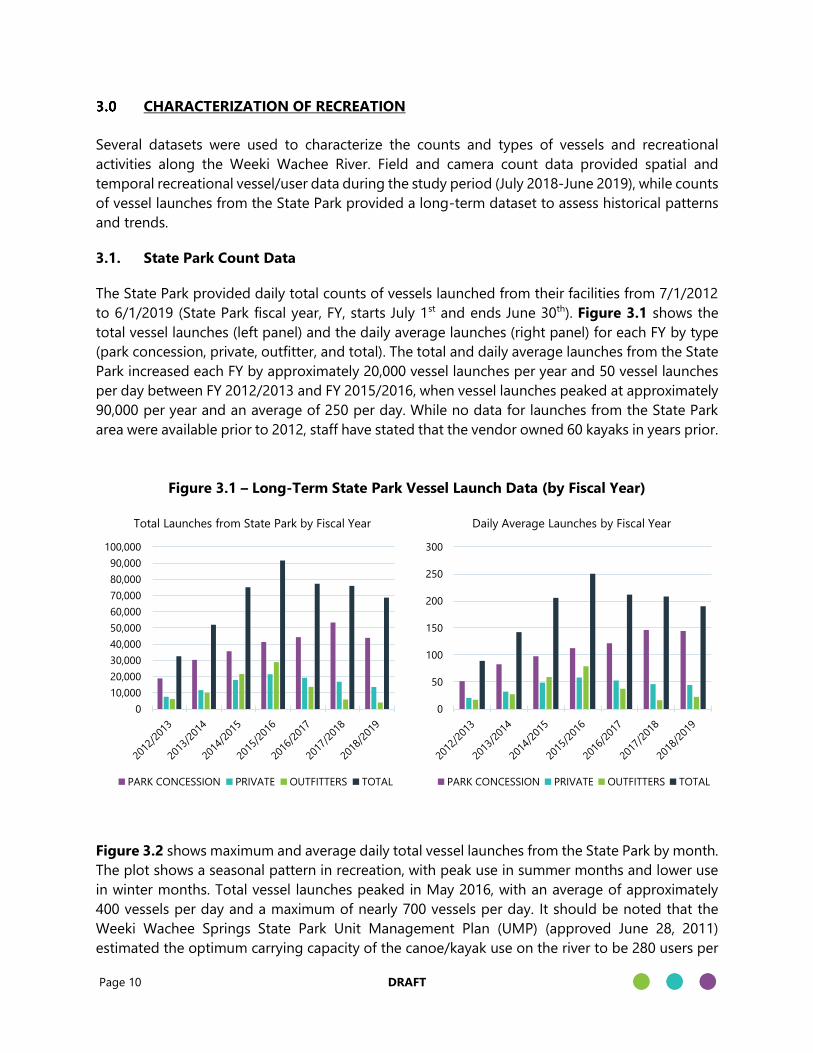
to 6/1/2019 (State Park fiscal year, FY, starts July 1st and ends June 30th). Figure 3.1 shows the
total vessel launches (left panel) and the daily average launches (right panel) for each FY by type
(park concession, private, outfitter, and total). The total and daily average launches from the State
Park increased each FY by approximately 20,000 vessel launches per year and 50 vessel launches
per day between FY 2012/2013 and FY 2015/2016, when vessel launches peaked at approximately
90,000 per year and an average of 250 per day. While no data for launches from the State Park
area were available prior to 2012, staff have stated that the vendor owned 60 kayaks in years prior.
Figure 3.1 – Long-Term State Park Vessel Launch Data (by Fiscal Year)
Figure 3.2 shows maximum and average daily total vessel launches from the State Park by month.
The plot shows a seasonal pattern in recreation, with peak use in summer months and lower use
in winter months. Total vessel launches peaked in May 2016, with an average of approximately
400 vessels per day and a maximum of nearly 700 vessels per day. It should be noted that the
Weeki Wachee Springs State Park Unit Management Plan (UMP) (approved June 28, 2011)
estimated the optimum carrying capacity of the canoe/kayak use on the river to be 280 users per
0
50
100
150
200
250
300
Daily Average Launches by Fiscal Year
PARK CONCESSION PRIVATE OUTFITTERS TOTAL
0
10,000
20,000
30,000
40,000
50,000
60,000
70,000
80,000
90,000
100,000
Total Launches from State Park by Fiscal Year
PARK CONCESSION PRIVATE OUTFITTERS TOTAL

Page 11 DRAFT
day6, which is approximately equivalent to 192 vessels per day (calculated from a regression
equation using Wood study data of kayaks and canoes vs. users: Users = 1.46*Vessels). A change
to the way the UMP was being enforced occurred on October 2018. Additionally, the disposables
ban went into effect in January 2019. The new enforcements occurred later during the study and
may have reduced the number of vessels that launched from the State Park. But it is unknown
what other factors may have also led to the reduction from previous years.
Figure 3.2 – State Park Daily Total Vessels (Max and Average Monthly Values)
3.2. Field Count Data
3.2.1 Total Counts
During 9 sampling events, Wood field staff tracked the number of users and vessels that passed
each sampling location, as well as the direction they were headed (upstream or downstream). The
total daily vessel passes observed on each sampling day are shown in Figure 3.3. Note that the
total daily counts include vessels passing the sampling station in both directions, as this provides
quantification of the total activity near the point bar. Therefore, vessels/users who travel in both
the upstream and downstream direction are counted twice in the total counts. During the high
recreation season (May-September), approximately 200-400 vessels per day passed by the upper
sampling sites, WW1, WW2, and WW3, while approximately 700-1000 vessels passed by the
furthest downstream sampling site, WW4. In the lower recreation season (October-April),
approximately 50-200 vessels per day passed the upper stations, while 100-400 vessels per day
6 The basis for this recommendation was not provided in the 2011 State Park Unit Management Plan.
0
100
200
300
400
500
600
700
Vess
els
(p
er
Day b
y M
on
rh)
Date
Maximum Daily Vessels Average Daily Vessels

Page 12 DRAFT
passed the downstream station. The daily total number of vessel passes was tightly correlated
with the daily total number of users (Users = 1.46*Vessels, R2=0.99) and therefore following a
similar distribution. Appendix B shows the total daily users observed on each sampling day.
Figure 3.3 – Daily Total Number of Vessel Passes by Sample Site
3.2.2 Travel Direction
While the total count of vessels or users traveling upstream and downstream provides
quantification of the total activity near the point bar, the truest count of individual vessels on the
river is the number of vessels traveling downstream since almost all users/vessels traveling
upstream must come back downstream. As shown in Figure 3.4, station WW4, the furthest
downstream site, had the most vessels that traveled upstream (mostly from Rogers Park, other
commercial vendor locations or private launch areas). On average, 50% of vessels and 54% of
users were travelling upstream at WW4, while WW1 had the least vessels/users travelling
upstream (3%). This finding highlights that any limits set to curb recreational use on the river
should also consider enforcement downstream at Rogers Park and other vendor locations in
addition to the State Park launch restrictions. Additional figures in Appendix B show the
distribution of downstream versus upstream vessels by site and by sampling event.
0
200
400
600
800
1000
WW1 WW2 WW3 WW4
Nu
mb
er o
f V
esse
l Pas
ses
7/5/2018 8/7/2018 9/3/2018 10/2/2018 12/19/2018
2/19/2019 4/24/2019 5/27/2019 6/24/2019

Page 13 DRAFT
Figure 3.4 – Percent of Vessels and Users Traveling Upstream at Each Station
3.2.3 Vessel Type
The type of vessel (kayak, canoe, paddleboard, motorboat, or other) was also noted during field
counts, and the overall percent of each vessel type (left panel) and percent of users in each vessel
type (right panel) over all stations and for all events are shown in Figure 3.5. It should be noted
that these values include the number of users/vessels observed at each sampling location
traveling in the downstream direction only (which is a truer representation of total people on the
river on a given day). Additional figures in Appendix B show the detailed distribution of vessel
types by site and sampling event and the average percent of vessel types per site. The number of
motorboats traveling only downstream is also shown in Appendix B. Additionally, Table 3.1
shows the average number of users per vessel type, calculated with user and vessel data collected
at all sample locations during the sampling events. Motorboats had the highest number of users
per vessel while paddleboards had the fewest.
The data show that kayaks are the dominant vessel type used on the Weeki Wachee River. At the
upstream sampling locations (WW1 and WW2), 90% of all vessels were kayaks, followed by 8%
paddle boards and 1-2% canoes and motorboats. The downstream stations (WW3 and WW4) are
closer to areas with access to boat ramps such as Rogers Park, Weeki Wachee Marina, and
privately-owned docks along the river and canals where visitors can launch motorboats. For the
most part, there is not much restriction other than boat rental availability or the number of
available trailer parking spots for privately owned boats that are non-river residents. Even at these
downstream stations, kayaks made up approximately 85% of all vessels, with paddleboards at 7%,
motorboats at 3%, and canoes at 2%. Averaging across all stations and events, motorboats made
up approximately 2% of all vessels on the river, but they do transport over twice as many users as
kayaks on a per vessel basis. Overall, users traveling by motorboat made up approximately 5% of
all users on the river.
3%6%
13%
50%
3%7%
17%
54%
0%
10%
20%
30%
40%
50%
60%
WW1 WW2 WW3 WW4
Perc
en
t Tra
vellin
g U
pst
ream
Average Vessels Average Users

Page 14 DRAFT
Figure 3.5 – Overall Percentage of Vessel and User Types from Field Count Data
Note: Values are overall averages for all stations using only downstream travel direction data.
Table 3.1 – Average Number of Users per Vessel Type
Vessel Type Average Number of Users/Vessel
Kayak 1.5
Canoe 2.5
Motorboat 3.4
Paddleboard 1.1
3.2.4 Motorboat Engine Size
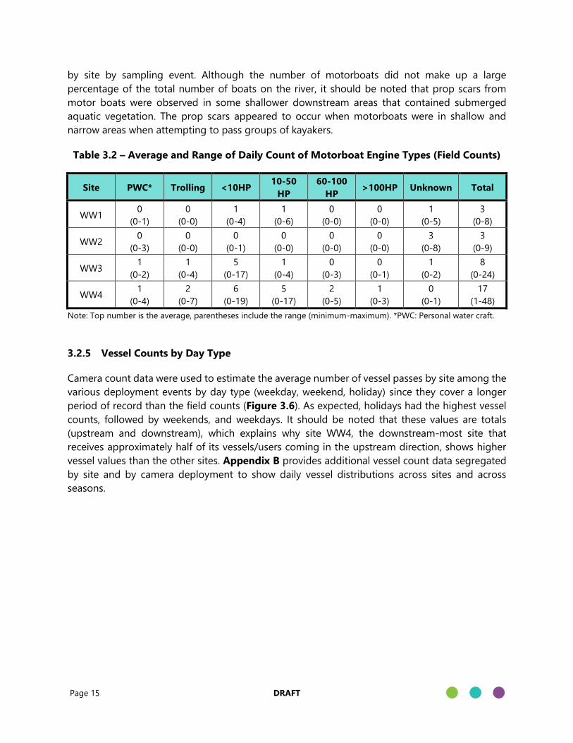
Another metric counted during field sampling events was the size of motors on motorboats. Table
3.2 summarizes the average daily count of each motorboat engine type observed at each site. The
motor sizes most commonly observed were less than 10 horsepower (hp), followed closely by 10-
50 hp. Note that the Weeki Wachee Marina rents out boats with a 9.9 hp engine, and these were
commonly observed at WW4 (the downstream-most sampling site). Larger motors, some with
more than 100 hp were observed, but only at the downstream stations. It should be noted that
the data used in this assessment were adjusted for vessels returning downstream, to avoid double-
counting motorboats. Appendix B provides a further breakdown of observed motorboat engines
87%
2%
2%8% 1%
Percent by Vessel Type
%of Kayak Vessels % of Canoe Vessels
% of Motorboats % of Paddleboards
% of Other Vessels
87%
3%
5%5% 0%
Percent by Users in Vessel Type
%of Kayak Users % of Canoe Users
% of Motorboat Users % of Paddleboard Users
% of Other Users
Page 15 DRAFT
by site by sampling event. Although the number of motorboats did not make up a large
percentage of the total number of boats on the river, it should be noted that prop scars from
motor boats were observed in some shallower downstream areas that contained submerged
aquatic vegetation. The prop scars appeared to occur when motorboats were in shallow and
narrow areas when attempting to pass groups of kayakers.
Table 3.2 – Average and Range of Daily Count of Motorboat Engine Types (Field Counts)
Site PWC* Trolling <10HP 10-50
HP
60-100
HP >100HP Unknown Total
WW1 0
(0-1)
0
(0-0)
1
(0-4)
1
(0-6)
0
(0-0)
0
(0-0)
1
(0-5)
3
(0-8)
WW2 0
(0-3)
0
(0-0)
0
(0-1)
0
(0-0)
0
(0-0)
0
(0-0)
3
(0-8)
3
(0-9)
WW3 1
(0-2)
1
(0-4)
5
(0-17)
1
(0-4)
0
(0-3)
0
(0-1)
1
(0-2)
8
(0-24)
WW4 1
(0-4)
2
(0-7)
6
(0-19)
5
(0-17)
2
(0-5)
1
(0-3)
0
(0-1)
17
(1-48)
Note: Top number is the average, parentheses include the range (minimum-maximum). *PWC: Personal water craft.
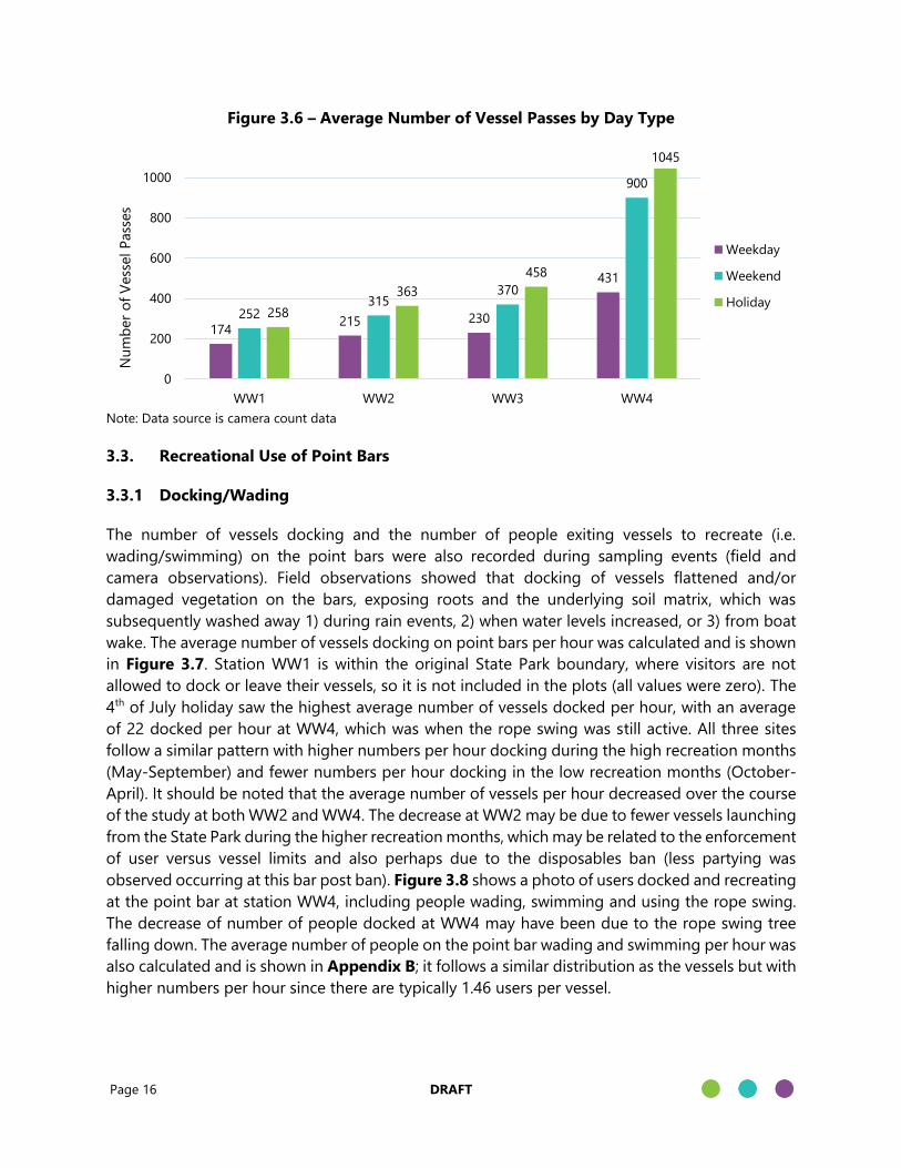
3.2.5 Vessel Counts by Day Type
Camera count data were used to estimate the average number of vessel passes by site among the
various deployment events by day type (weekday, weekend, holiday) since they cover a longer
period of record than the field counts (Figure 3.6). As expected, holidays had the highest vessel
counts, followed by weekends, and weekdays. It should be noted that these values are totals
(upstream and downstream), which explains why site WW4, the downstream-most site that
receives approximately half of its vessels/users coming in the upstream direction, shows higher
vessel values than the other sites. Appendix B provides additional vessel count data segregated
by site and by camera deployment to show daily vessel distributions across sites and across
seasons.
Page 16 DRAFT
Figure 3.6 – Average Number of Vessel Passes by Day Type
Note: Data source is camera count data
3.3. Recreational Use of Point Bars
3.3.1 Docking/Wading
The number of vessels docking and the number of people exiting vessels to recreate (i.e.
wading/swimming) on the point bars were also recorded during sampling events (field and
camera observations). Field observations showed that docking of vessels flattened and/or
damaged vegetation on the bars, exposing roots and the underlying soil matrix, which was
subsequently washed away 1) during rain events, 2) when water levels increased, or 3) from boat
wake. The average number of vessels docking on point bars per hour was calculated and is shown
in Figure 3.7. Station WW1 is within the original State Park boundary, where visitors are not
allowed to dock or leave their vessels, so it is not included in the plots (all values were zero). The
4th of July holiday saw the highest average number of vessels docked per hour, with an average
of 22 docked per hour at WW4, which was when the rope swing was still active. All three sites
follow a similar pattern with higher numbers per hour docking during the high recreation months
(May-September) and fewer numbers per hour docking in the low recreation months (October-
April). It should be noted that the average number of vessels per hour decreased over the course
of the study at both WW2 and WW4. The decrease at WW2 may be due to fewer vessels launching
from the State Park during the higher recreation months, which may be related to the enforcement
of user versus vessel limits and also perhaps due to the disposables ban (less partying was
observed occurring at this bar post ban). Figure 3.8 shows a photo of users docked and recreating
at the point bar at station WW4, including people wading, swimming and using the rope swing.
The decrease of number of people docked at WW4 may have been due to the rope swing tree
falling down. The average number of people on the point bar wading and swimming per hour was
also calculated and is shown in Appendix B; it follows a similar distribution as the vessels but with
higher numbers per hour since there are typically 1.46 users per vessel.
174215 230
431
252315
370
900
258
363
458
1045
0
200
400
600
800
1000
WW1 WW2 WW3 WW4
Nu
mb
er
of
Vess
el P
ass
es
Weekday
Weekend
Holiday

Page 17 DRAFT
Figure 3.7 – Average Number of Vessels Docked Per Hour by Site
Figure 3.8 – Rope Swing, Docked Vessels, and People Wading and Swimming at WW4
Figure 3.9 shows the percentage of passing vessels that docked at each point bar. The number
of vessels docked per people wading and swimming are notably higher during the higher
recreation season, but the percentage of vessels docking remains relatively stable throughout the
year at WW2 and WW3. Station WW2 had the highest percentage of passing vessels that docked
on the point bar (between 20% and 40%), likely because it was directly downstream of the original
0
5
10
15
20
25
WW2 WW3 WW4
Nu
mb
er o
f V
esse
ls D
ock
ed (
Ho
url
y A
vg)
7/5/2018 8/7/2018 9/3/2018 10/2/2018 12/19/2018
2/19/2019 4/24/2019 5/27/2019 6/24/2019
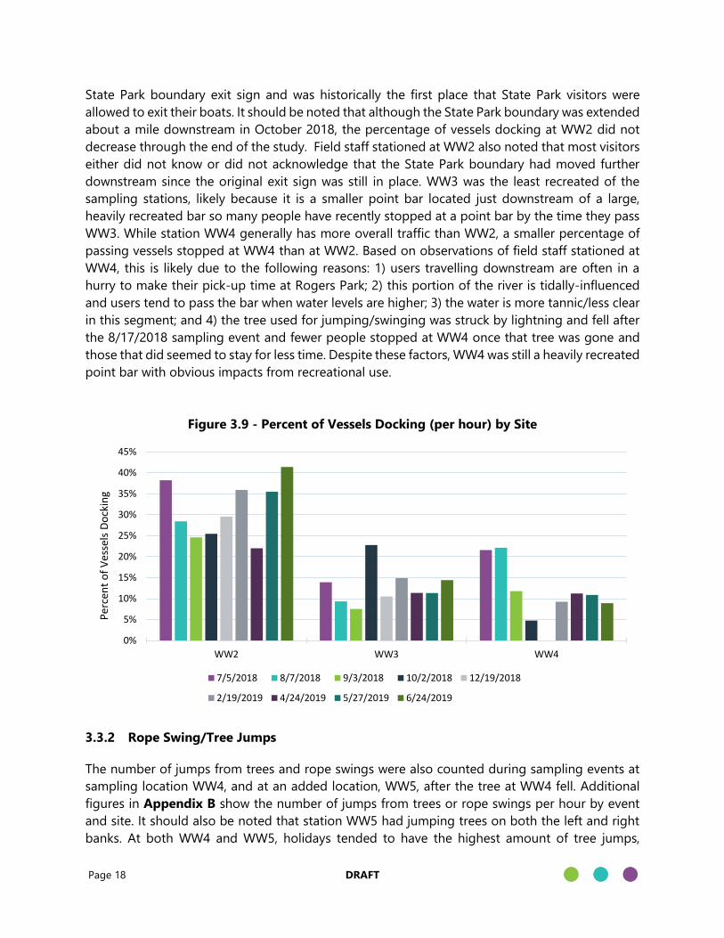
Page 18 DRAFT
State Park boundary exit sign and was historically the first place that State Park visitors were
allowed to exit their boats. It should be noted that although the State Park boundary was extended
about a mile downstream in October 2018, the percentage of vessels docking at WW2 did not
decrease through the end of the study. Field staff stationed at WW2 also noted that most visitors
either did not know or did not acknowledge that the State Park boundary had moved further
downstream since the original exit sign was still in place. WW3 was the least recreated of the
sampling stations, likely because it is a smaller point bar located just downstream of a large,
heavily recreated bar so many people have recently stopped at a point bar by the time they pass
WW3. While station WW4 generally has more overall traffic than WW2, a smaller percentage of
passing vessels stopped at WW4 than at WW2. Based on observations of field staff stationed at
WW4, this is likely due to the following reasons: 1) users travelling downstream are often in a
hurry to make their pick-up time at Rogers Park; 2) this portion of the river is tidally-influenced
and users tend to pass the bar when water levels are higher; 3) the water is more tannic/less clear
in this segment; and 4) the tree used for jumping/swinging was struck by lightning and fell after
the 8/17/2018 sampling event and fewer people stopped at WW4 once that tree was gone and
those that did seemed to stay for less time. Despite these factors, WW4 was still a heavily recreated
point bar with obvious impacts from recreational use.
Figure 3.9 - Percent of Vessels Docking (per hour) by Site
3.3.2 Rope Swing/Tree Jumps
The number of jumps from trees and rope swings were also counted during sampling events at
sampling location WW4, and at an added location, WW5, after the tree at WW4 fell. Additional
figures in Appendix B show the number of jumps from trees or rope swings per hour by event
and site. It should also be noted that station WW5 had jumping trees on both the left and right
banks. At both WW4 and WW5, holidays tended to have the highest amount of tree jumps,
0%
5%
10%
15%
20%
25%
30%
35%
40%
45%
WW2 WW3 WW4
Per
cen
t o
f V
esse
ls D
ock
ing
7/5/2018 8/7/2018 9/3/2018 10/2/2018 12/19/2018
2/19/2019 4/24/2019 5/27/2019 6/24/2019

Page 19 DRAFT
reaching up to 47 jumps in one hour. During the remaining events, the frequency of tree jumps
tended to peak between noon and 13:00 with 10-30 jumps per hour. As previously mentioned,
the absence of the rope swing tree at WW4 appears to have had a direct effect on the number of
users docking at the bar. While many users still utilized the bar for recreation, they did not tend
to stay as long or stop as frequently. It can also be seen from Figure 3.10 that the tree roots are
uncovered in both photos, which is likely due to trampling along the bar to access the rope swing
on the tree.
Figure 3.10 – Rope Swing at Site WW4 Before and After Tree Fall
3.4. Social Surveys
Field staff at the downstream-most sampling sites (WW4 and WW5) conducted exit interviews
with randomly selected groups of visitors using a standard set of questions (provided in Appendix
B). Over the course of the study, 82 groups (327 individuals) were interviewed. Up to 10 interviews
were conducted per field sampling day, which were spread throughout the day. Of the surveyed
groups, visitors noted similar recreational reasons for stopping on point bars, such as picnicking,
swimming, and taking a break from travelling in their respective vessels. Visitors reported to enjoy
the river, suggesting that they would recommend the Weeki Wachee River as a place to view
wildlife and the crystal-clear water. Those with negative comments about their experience noted
that there were too many people on the river. In general, visitors in motorboats complained there

Page 20 DRAFT
were too many inexperienced kayakers on the river, while kayakers complained there were too
many inexperienced motorboat drivers on the river. When asked about the rope swings, not many
of the people interviewed had used them due to safety concerns. Several long-time visitors
noticed changes in submerged aquatic vegetation and an increase in the number of visitors over
the years. Summarized survey results are provided in Table 3.3.
Table 3.3 – Summary of Social Survey Responses
Survey Metric Percent of Total Surveyed
First time groups 38%
Returning groups 70%
Groups sharing returning and first-time users 7%
Users launching before noon 99%
Users renting watercrafts 59%
Users owning watercrafts 41%
Users docking under 30 minutes 62%
Users docking over 30 minutes 17%
Users that did not dock 12%
Users launching from Weeki Wachee State Park 39%
Users launching from Rogers Park or Kayak Shack 30%
Users launching from Weeki Wachee Marina 4%
Users launching from SUP Weeki 1%
Users launching from private residences 9%
Users reporting human & boat congestion 25%
Hernando County residents reporting congestion 8%
3.5. Summary of Recreational Activities
Data collected by Wood during 9 sampling events between July 2018 and June 2019 found that
during the higher recreation season (May-September), the number of vessels observed per day
along the Weeki Wachee River ranged between approximately 200 and 600, with higher numbers
of vessels being observed at the downstream end, nearer to Rogers Park. During the lower-
recreation season, (October-April), fewer total vessels were observed per day, ranging from
approximately 50 to 200. The highest counts were observed on holidays, followed by weekends
and weekdays. While total vessel and user numbers are important for quantifying impacts to the
river system, it is also important to note that these totals include travelers going in both directions.
Looking at the downstream only direction provides the most accurate count of the number of
vessels/users on the river in a given day because those travelling upstream must come back
downstream. Near the State Park, only between 3 to10% of the vessels observed were travelling
upstream, while in the lower reaches of the river, near Rogers Park, approximately half of the vessel
traffic was travelling upstream indicating that approximately half the users observed at WW4 came
from the State Park and half came from Rogers Park, private river-access residences or from
Page 21 DRAFT
downstream vendors. At all stations, the majority of vessel traffic was composed of kayaks (85-
90%), while paddleboards, motorboats, and canoes make up 7-8%, 1-4%, and 1-3%, respectively.
The highest number of motorboats were observed at the downstream-most station (WW4), with
the most common motor sizes observed being less than 10 horsepower (hp), followed closely by
10-50 hp. The highest number of vessels docking and users wading/swimming per hour was
observed at the downstream-most station (WW4), but the highest percent of passing vessels that
docked occurred at the historic State Park exit (WW2). Data and observations also showed that
visitors jumped from trees up to 40 times per hour and that jumping trees/rope swings contribute
to the popularity of a bar as a docking location and damage to the point bar from trampling. From
the social surveys, it appears that approximately 40% of users launch from upstream at the State
Park, while 30% launch from downstream at Rogers Park or Kayak Shack, and the remainder launch
from various marinas and private residences on the downstream end of the river. While it appears
that many visitors believe the river is crowded, they also do enjoy the clear waters and natural
systems of Weeki Wachee.
Page 22 DRAFT
FLUVIAL GEOMORPHOLOGY ASSESSMENT
Fluvial geomorphology can be described as the interaction of flowing water with its environment;
which affects channel shape and size, bed substrate, flow, velocity, vegetation, and river corridor
ecology and biodiversity. Many factors influence the geomorphology of a stream, including
climate, soil types, groundwater influence, topography, vegetation, land use in the contributing
watershed, and activities within the stream or along the streambanks. The discipline of fluvial
geomorphology can help to understand the processes occurring within a stream system. Various
fluvial geomorphic assessments were performed as part of this study to assess whether the Weeki
Wachee River diverges from expected self-sustaining characteristics, and to assess whether
divergence can be linked to recreation. These included an aerial point bar interpretation (Task
2.1), recreational trampling assessment (Task 2.3), comparative site assessment (Task 2.1),
cumulative assessment (Task 2.2), and assessment of leaning trees as described in the subsequent
sections. Map 4 shows the locations of the point bars used in each analysis.
4.1. Aerial Point Bar Interpretation
Point bars with clear expanses of beach-like sand are a recreational draw for visitors to the Weeki
Wachee River; however, these are not normally observed in Florida spring runs. While the natural
bed material of the Weeki Wachee River is comprised predominantly of sand, point bars in Florida
spring runs generally support herbaceous vegetation and subsequently accumulate organic soils
on the bar. An assessment of vegetative cover over the past decade at selected point bars within
the Weeki Wachee River was conducted to observe whether a pattern of progressive vegetation
and organic soil loss has occurred.
4.1.1 Methodology
Using aerial imagery from Google Earth Pro software (image source Landsat/Copernicus),
apparent changes in vegetation and morphology on selected point bars were observed through
time. The 6 point bars used in aerial interpretation were selected because they had the clearest
views of bar vegetation in the available aerials over the last decade. The vegetated area of each
bar was calculated by setting reference points at the forested edge and tracing the vegetated
limits of the exposed sand of the bar. Vegetated area did not include submerged aquatic
vegetation or algae, and approximations aimed to account for overhanging trees. The vegetated
areas for each year with a clear aerial image were compared to calculate a change in vegetative
cover.
4.1.2 Results
Figure 4.1 shows the point bar at Wood Station WW2 (the historic exit of the State Park) in 2008
compared to 2017, and the vegetation loss of approximately 1600 ft2. This side by side comparison
clearly shows the magnitude of vegetation and subsequent organic soil loss at this point bar, and
kayaks can even be seen docked in the 2017 image on the right. Figure 4.2 shows the cumulative
percent reduction in vegetation among all 6 point bars assessed compared to the average daily
vessels launched from the State Park in each fiscal year (FY 2012/2013 plotted as 2013, etc.). State
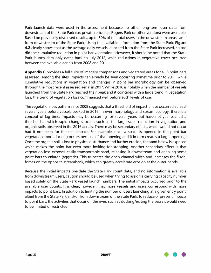
Page 23 DRAFT
Park launch data were used in the assessment because no other long-term user data from
downstream of the State Park (i.e. private residents, Rogers Park or other vendors) were available.
Based on previously discussed results, up to 50% of the total users in the downstream areas came
from downstream of the State Park. Using the available information from the State Park, Figure
4.2 clearly shows that as the average daily vessels launched from the State Park increased, so too
did the cumulative reduction in point bar vegetation. However, it should be noted that the State
Park launch data only dates back to July 2012, while reductions in vegetative cover occurred
between the available aerials from 2008 and 2011.
Appendix C provides a full suite of imagery comparisons and vegetated areas for all 6 point bars
assessed. Among the sites, impacts can already be seen occurring sometime prior to 2011, while
cumulative reductions in vegetation and changes in point bar morphology can be observed
through the most recent assessed aerial in 2017. While 2016 is notably when the number of vessels
launched from the State Park reached their peak and it coincides with a large trend in vegetation
loss, the trend of vegetation loss commenced well before such levels of use.
The vegetation loss pattern since 2008 suggests that a threshold of impactful use occurred at least
several years before vessels peaked in 2016. In river morphology and stream ecology, there is a
concept of lag time. Impacts may be occurring for several years but have not yet reached a
threshold at which rapid changes occur, such as the large-scale reduction in vegetation and
organic soils observed in the 2016 aerials. There may be secondary effects, which would not occur
had it not been for the first impact. For example, once a space is opened in the point bar
vegetation, more docking occurs because of that opening and it in turn creates a larger opening.
Once the organic soil is lost to physical disturbance and further erosion, the sand below is exposed
which makes the point bar even more inviting for stopping. Another secondary effect is that
vegetation loss exposes easily transportable sand, releasing it downstream and enabling some
point bars to enlarge (aggrade). This truncates the open channel width and increases the fluvial
forces on the opposite streambank, which can greatly accelerate erosion at the outer bends.
Because the initial impacts pre-date the State Park count data, and no information is available
from downstream users, caution should be used when trying to assign a carrying capacity number
based solely on the State Park vessel launch numbers. The initial impacts occurred prior to the
available user counts. It is clear, however, that more vessels and users correspond with more
impacts to point bars. In addition to limiting the number of users launching at a given entry point,
albeit from the State Park and/or from downstream of the State Park, to reduce or prevent impacts
to point bars, the activities that occur on the river, such as docking/exiting the vessels would need
to be limited or restricted.

Page 24 DRAFT
Figure 4.1 – Reduction in Vegetation from 2008 to 2017 at Weeki Wachee Point Bar 1
Note: All historic Landsat/Copernicus aerial imagery obtained from Google Earth Pro
Figure 4.2 – Cumulative Percent Reduction of Vegetation on Point Bars Compared to
Average Daily State Park Vessel Launches
Note: Cumulative vegetation reduction is calculated as (vegetated area in year X – vegetated area in 2008)/vegetated
area in 2008. The earliest State Park vessel launch data begins in June 2012. Point bar locations shown in Map 4.
2008 2009 2010 2011 2012 2013 2014 2015 2016 2017
0
50
100
150
200
250
300
0%
5%
10%
15%
20%
25%
30%
35%
2008 2009 2010 2011 2012 2013 2014 2015 2016 2017
Average Daily Vessels Bar 1 (WW2) Bar 6 Bar 21 Bar 22 Bar 24 Bar 28
Year
Cu
mu
lati
ve
Veg
eta
tio
n R
ed
uct
ion
(%
)
Avera
ge D
aily V
ess
els
fro
m S
tate
Park

Page 25 DRAFT
4.2. Experimental Recreational Trampling Assessment
An experimental trampling assessment was conducted to measure the impact, intensity of
recreational disturbance, and potential recovery of plant communities and soils within the Weeki
Wachee River. Disturbances caused by trampling events often have extensive implications for the
health and function of natural ecosystems. Studies involving even low levels of visitor traffic on
natural systems have shown that recreational trampling can have negative effects on vegetation
and soils (Jägerbrand and Alatalo 2015; Pertierra et al. 2013). Commonly documented effects on
vegetation include changes in species diversity, composition, growth patterns, percent cover and
an increased abundance of opportunistic and rapidly colonizing invasive species (Cole 2004; Kuss
and Hall 1991; Pickering and Growcock 2009). Concurrent changes to soil compaction and water-
holding capacity can also lead to erosional sources of sediment transport and sedimentation,
decreased water clarity, and loss of submerged aquatic vegetation within the river. Vegetative
controls on spring run morphology are significant in preserving the key functions and health of
riverine ecosystems such as the Weeki Wachee River (Kiefer et al. 2015).
4.2.1 Methodology
A total of 3 point bars with intact herbaceous vegetation were selected at random for the
experimental trampling assessment (Map 4). These sites were located within the previous State
Park boundary where vessels are not supposed not dock and clear impacts to point bar vegetation
were not observed. The initial trampling event was conducted on 5/28/2019, with a two-week
follow-up site visit to assess immediate impacts on 6/12/2019, and a 6-month interim follow-up
site visit to assess potential reestablishment within the recovery period on 11/24/2019. Additional
follow-up site visits at the one-year mark (May 2020) and two-year marks (May 2021) since
trampling should also be conducted to assess potential recovery from trampling. It is important
to note that the trampling event occurred during low water levels, and the bar substrates were
merely saturated and not under standing water. Therefore, the recovery assessments should also
occur during similar hydrologic conditions. The interim reestablishment assessment in November
2019 occurred during high water levels and the bars were all under almost a foot of water. The
information gleaned from the interim assessment provided good information on how the bars
were beginning to recover under varying hydrologic conditions, which are important for
management considerations.
Adapting methodology from Cole and Bayfield (1993), five equally-dimensioned lanes (Figure
4.3) of different trampling intensities, each with two subplots, were identified on each of the three
experimental point bars. Upon site selection, pin flags were placed at each subplot corner and
photographs documenting vegetation cover and height were taken. Photographs of trampling
sites with applied treatments, and their respective soil profiles can be found in Appendix D.
Percent vegetation cover and species type along with soil matrix profiles were identified for each
subplot (10 subplots per bar) prior to trampling. Percent cover was recorded as 0, 0.2 (if between
0 and 0.5%), 1, 5, 10, 15, 20, 30, 40, 50, 60, 70, 80, 90 or 100% for vegetation, with the same
percentage categories used for dead vegetation and bare soils. One soil matrix profile was taken

Page 26 DRAFT
within each subplot using a tubular soil sampler to document the thickness and type of overlaying
soil layers. Soil types were documented as detritus, peat, muck, sand, silt, clay, combinations or
other when present in the upper 30 cm of the soil core.
Each of the 5 lanes was randomly assigned a trampling intensity (0, 25, 50, 100, or 200 passes),
with one pass defined as walking at a natural gait in one direction. Trampling was performed by
the same individual to provide consistency across sites. After receiving the designated intensity of
trampling, the immediate effects to soil and vegetation were recorded and photographed.
Signage informing that the site was restricted was placed onto construction fencing that was held
up by steel rebar was installed as a barrier at each trampling site to restrict site access to the
research plots (Figure 4.4).
Figure 4.3 – Layout of Recreational Trampling Assessment Lanes
Cole and Bayfield (1993)
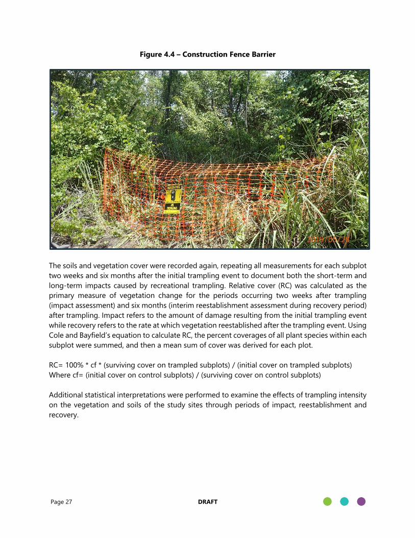
Page 27 DRAFT
Figure 4.4 – Construction Fence Barrier
The soils and vegetation cover were recorded again, repeating all measurements for each subplot
two weeks and six months after the initial trampling event to document both the short-term and
long-term impacts caused by recreational trampling. Relative cover (RC) was calculated as the
primary measure of vegetation change for the periods occurring two weeks after trampling
(impact assessment) and six months (interim reestablishment assessment during recovery period)
after trampling. Impact refers to the amount of damage resulting from the initial trampling event
while recovery refers to the rate at which vegetation reestablished after the trampling event. Using
Cole and Bayfield’s equation to calculate RC, the percent coverages of all plant species within each
subplot were summed, and then a mean sum of cover was derived for each plot.
RC= 100% * cf * (surviving cover on trampled subplots) / (initial cover on trampled subplots)
Where cf= (initial cover on control subplots) / (surviving cover on control subplots)
Additional statistical interpretations were performed to examine the effects of trampling intensity
on the vegetation and soils of the study sites through periods of impact, reestablishment and
recovery.
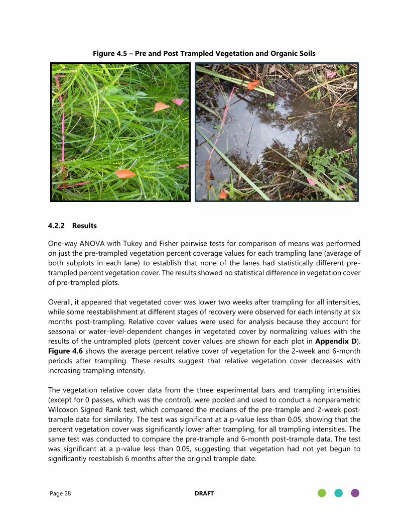
Page 28 DRAFT
Figure 4.5 – Pre and Post Trampled Vegetation and Organic Soils
4.2.2 Results
One-way ANOVA with Tukey and Fisher pairwise tests for comparison of means was performed
on just the pre-trampled vegetation percent coverage values for each trampling lane (average of
both subplots in each lane) to establish that none of the lanes had statistically different pre-
trampled percent vegetation cover. The results showed no statistical difference in vegetation cover
of pre-trampled plots.
Overall, it appeared that vegetated cover was lower two weeks after trampling for all intensities,
while some reestablishment at different stages of recovery were observed for each intensity at six
months post-trampling. Relative cover values were used for analysis because they account for
seasonal or water-level-dependent changes in vegetated cover by normalizing values with the
results of the untrampled plots (percent cover values are shown for each plot in Appendix D).
Figure 4.6 shows the average percent relative cover of vegetation for the 2-week and 6-month
periods after trampling. These results suggest that relative vegetation cover decreases with
increasing trampling intensity.
The vegetation relative cover data from the three experimental bars and trampling intensities
(except for 0 passes, which was the control), were pooled and used to conduct a nonparametric
Wilcoxon Signed Rank test, which compared the medians of the pre-trample and 2-week post-
trample data for similarity. The test was significant at a p-value less than 0.05, showing that the
percent vegetation cover was significantly lower after trampling, for all trampling intensities. The
same test was conducted to compare the pre-trample and 6-month post-trample data. The test
was significant at a p-value less than 0.05, suggesting that vegetation had not yet begun to
significantly reestablish 6 months after the original trample date.

Page 29 DRAFT
Linear regression plots (in Appendix D) for each trample site show a positive relationship between
trampling intensity and reduction in percent of vegetation cover. To assess differences in effects
of trampling intensities, one-way ANOVA with Tukey and Fisher pairwise tests along with a
Dunnett Multiple Comparisons test (with trampling intensity 0 as the control) were performed on
the relative cover of vegetation dataset (2-weeks and 6-months after trampling). For the 2-week
post-trampled dataset, the Fisher test for difference in means showed that relative cover was
significantly less (at alpha=0.05) than the control at a trampling intensity of 200, but not at
intensities of 25, 50, or 100. For the 6-month post-trampled dataset, the Tukey and Dunnett
comparisons tests showed that relative cover was significantly less (at alpha=0.05) than the control
at trampling intensities of 100 and 200, and the Fisher comparison test showed that relative cover
was significantly less than the control at trampling intensities of 50, 100, and 200. Overall, based
on the various statistical analyses, the higher trampling intensities showed greater reductions in
relative vegetation coverage.
Figure 4.6 – Percent Relative Cover Two Weeks and Six Months After Trampling (Average
of All Trample Bars)
Figures 4.7 - 4.9 show the relationship between relative cover and the intensity of trampling
received to the study site after the initial 2-week period (impact) and 6-month period (interim
reestablishment). Impact is defined as 2 weeks after trampling because it leaves sufficient time to
observe plant deaths due to trampling (as opposed to immediately after trampling when
vegetation still appear alive, but flattened). After the 2-week impact period, the recovery period
begins with some reestablishment of mostly opportunistic invasive vegetation, and the first
interim recovery observations were taken at 6 months. It should be noted that recovery may take
much longer than 6 months (depending on environmental and seasonal factors), and that 12-
month recovery data will be collected, although it will occur outside of the carrying capacity study
contract period. Overall, after the initial 2-week trampling event, percent relative cover decreased
in response to the increasing trampling intensity across all 3 bars.
0%
10%
20%
30%
40%
50%
60%
70%
80%
90%
100%
0 25 50 100 200Perc
en
t R
ela
tive
Co
ver
(Avera
ge o
f A
ll
Bars
)
Trampling Intensity
Two Weeks Post-Trample Six Months Post-Trample

Page 30 DRAFT
At the interim 6-month point in the recovery period, it appeared that the trampled plots were in
different stages of recovery, depending on their environments. Overall, it appeared that higher
water levels and onset of winter may have been limiting factors in vegetation recovery, as dead
and bare coverage, even in the un-trampled control lanes were observed at all bars. In addition
to these overall observations, each of the three bars appeared to have different recovery
responses. At Bar 1, where there is lower flow than at Bars 2 and 3, organic sediments had begun
collecting in the submerged trampled plots, but presumably high water levels prevented
reestablishment of many species that were present before trampling. On the bar that remained
above the waterline (Bar 2), the dead, trampled Cladium jamaicense (sawgrass) appeared to have
created a physical barrier (similar to mulch) on the top of many of the plots, potentially limiting
reestablishment of vegetation. Bar 3 was also submerged but located on an outer bend that
appears to receive higher flows/velocities than at Bar 1. At Bar 3, it appears that organic sediments
were not accumulating (presumably due to higher flows), however, floating vegetation such as
Pistia stratiotes had been transported by flow into the plots. Additionally, dense submerged
vegetation and vines (such as Najas guadalupensis, Diodia virginiana, and Mikania scandens) had
grown into the trampled plots that were originally dominated by larger emergent herbaceous
species (such as Typha sp. and Sagittaria lancifolia), which creates the appearance of a high
recovery (>100%) of total vegetation cover, but with different, ephemeral species. Therefore, at
the one-year mark, it will be important to assess the vegetation in terms of a more qualitative
metric such as types of communities that colonized, reestablished or recovered, rather than a total
percent coverage as a quantitative metric to assess recovery.
Figure 4.7 – Relative Cover After Impact and Reestablishment at Trample Bar 1
0%
10%
20%
30%
40%
50%
60%
70%
80%
90%
100%
0 25 50 100 200
Perc
en
t R
ela
tive C
over
Trample Intensity (Number of Passes)
Impact
Reestablishment

Page 31 DRAFT
Figure 4.8 – Relative Cover After Impact and Reestablishment at Trample Bar 2
Figure 4.9 – Relative Cover After Impact and Reestablishment at Trample Bar 3
Common vegetation described at trampling sites prior to trampling were primarily composed of
herbaceous vascular plants. Table 4.1 provides a list of dominant species at each trampling
location. Floating-leaf aquatic plants were noted as part of the vegetative survey but were not
used in the calculation of total percent cover.
0%
10%
20%
30%
40%
50%
60%
70%
80%
90%
100%
0 25 50 100 200
Perc
en
t R
ela
tive C
over
Trample Intensity (Number of Passes)
Impact
Reestablishment
0%
20%
40%
60%
80%
100%
120%
0 25 50 100 200
Perc
en
t R
ela
tive C
over
Trample Intensity (Number of Passes)
Impact
Reestablishment

Page 32 DRAFT
Table 4.1 – Dominant Vegetation at Trampling Sites
Trample Bar 1 Trample Bar 2 Trample Bar 3
Cyperus haspan Cladium jamaicense Typha sp.
Boehmeria cylindrica Cicuta maculata Sagittaria lancifolia
Cicuta maculata Vitis rotundifolia Ludwigia sp.
Hydrocotyle umbellata Cyperus haspan Polygonum sp.
Cladium jamaicense Colocasia esculenta Boehmeria cylindrica
Sagittaria lancifolia Ludwigia sp. Cicuta maculata
Mikania scandens Boehmeria cylindrica Micranthemum umbros
Alternanthera philoxeroides Toxicodendron radicans Diodia sp.
Bacopa monnieri Polygonum sp. Hydrocotyle umbellata
Colocasia esculenta Micranthemum umbros Mikania scandens
Cynodon dactylon Mikania scandens Pistia stratiotes*
Micranthemum umbros Pistia stratiotes*
*Pistia stratiotes is a floating leaf aquatic plant and was not included in percent cover values
The soil profile data collected before and two weeks after trampling were used to identify loss of
organic matter from recreational trampling. If there was substantial organic content in the top 6-
10 cm of the profile, the subplot was marked as “organics present”. If the core was primarily sand,
it was assigned “organics not present”. The binary dataset was used to perform McNemar’s test
(non-parametric statistical test), which tests whether paired proportions are significantly different
(i.e. if soils before trampling and 2 weeks after trampling were significantly different). When
comparing the soils before and 2 weeks after trampling, the test was significant with a p-value
less than 0.05 suggesting that organic soils decreased significantly after the initial trampling event.
The test was also significant (p-value <0.05) when comparing the soils before and 6 months after
trampling, suggesting that the organic soils were still significantly reduced 6 months after
trampling. When comparing the soils data 2 weeks after and 6 months after trampling, the test
was not significant, indicating that there was no significant loss or recovery of organic soils during
the 2-week and 6-month period. Overall, these results suggest that soils can be significantly
impacted within 2 weeks of trampling, and that those impacts may persist until at least 6 months
after trampling.
Trampling events at submerged bars were often subject to higher cases of soil disturbance than
events on non-submerged bars. It is worth noting that saturation of soils and/or depth of water
in trampling lane appears to intensify effects of trampling and potential for recovery. Wet soils
displace under foot and adhere to footwear, so vegetation is not only trampled, but can also be
uprooted and buried. Areas originally containing lower amounts of water, expressed increased
water pooling after the initial trampling, which is consistent with changes in soil compaction. In
the submerged point bars, disturbed soils from trampling also appeared to be more susceptible
to washout during rain events. It should also be noted that the submerged vegetation at the edge
of the bars appears to be especially susceptible to trampling because these water depths are
conducive to safely exiting a kayak (or other vessels).

Page 33 DRAFT
Turbidity was measured in triplicates and averaged at select bars to describe water clarity before
and after recreational trampling. As an undisturbed control, turbidity measurements were taken
from the boat above areas with clean sand and areas composed of mostly organics. Turbidity was
then measured at the same sites immediately after soils were disturbed by trampling activity, and
again after the sample had been allowed to settle for 5-10 minutes in a test jar. Table 4.2 and
Figure 4.10 show the measured values of turbidity at select bars.
Table 4.2 – Turbidity (NTU) Values at Trample Sites Before and After Trampling
Substrate Material
(Location)
Average Turbidity (NTU)
Undisturbed Post-Trample
(Immediate) Settled in Test Jar
Sand (Bar 23) 0.36 1.6 0.8
Organic (Bar 23) 0.57 164.9 30.0
Organic (Bar 21) 0.27 95.0 24.0
Figure 4.10 – Comparison of Turbidity (NTU) at Bar 21 and Bar 23
0
20
40
60
80
100
120
140
160
UndisturbedPost-Trample (Immediate) Settled in Test Jar
Tu
rbid
ity (
NTU
)
Sand (Bar 23) Organic (Bar 23) Organic (Bar 21)
Page 34 DRAFT
4.2.3 Summary of Recreational Trampling Assessment
The experimental trampling assessment provided documentation of vegetation and soil sensitivity
in select shoreline sites of the Weeki Wachee River. After the initial trampling event, each of the
three subplots showed increases in exposed soil and dead vegetation. As expected, areas trampled
at variable intensities were subject to fluctuating amounts of vegetation and soil disturbance.
Percent relative cover of vegetation declined substantially as trampling intensity increased after
the initial two-week and six-month trampling events. Percent relative cover was somewhat
variable at the six-month interim reestablishment event suggesting each subplot is at a different
stage of recovery influenced not only by trampling intensity, but multiple other environmental
variables. The reestablishment of vegetation after six months of recovery appeared to be
influenced by water level, flows, seasonal climate, and surrounding vegetation. Submerged bars
were often newly colonized by floating-leaf aquatic plants such as Pistia stratiotes and traveling
vines such as Mikania scandens, thus changing the community composition. Soil profiles taken
after initial impact showed decreases in surface organic matter, signifying disruptions from soil
compaction and disturbance. The loss of organic soils was significant two weeks after trampling,
and continued to be significant six months after trampling, with no significant change in presence
of organic soils between two weeks and six months.
Recreation-induced vegetation trampling has been shown to adversely impact the herbaceous
shoreline of the Weeki Wachee River. Limiting or fully restricting vessel docking along the
shorelines in general or setting up specific areas for docking and recreation at designated areas
that have been engineered for that purpose could decrease the amount of vegetation loss and
erosion along the river.
4.3. Comparative Site Assessment
4.3.1 Site Selection
Wood selected a spring-fed river containing point bars with intact vegetative cover to provide a
comparative reference site from which to assess ecological impacts observed at point bars on the
Weeki Wachee River (such as vegetation and organic soil loss). Candidate spring runs included
Alexander Springs Run and Juniper Spring Run in the Ocala National Forest and Rock Springs Run
in Orange County. These rivers were reviewed via aerial imagery and site visits to find a site with
similar fluvial geomorphic characteristics such as meander pattern, bend geometry, and
hydrologic regime to the Weeki Wachee River. Alexander Springs Run was selected as the
comparative site for the Weeki Wachee River because it had similar geomorphic patterns,
dimensions, and flow regime. It also displays fewer impacts from recreation versus Rock Springs
Run, which is heavily eroding in some areas. While the Alexander Springs Run in the studied
section is not entirely pristine (it has some rope swings, docks, short segments of cleared shoreline,
an eroded kayak/small boat launch, and an actively eroded bluff), it has numerous vegetated and
intact bars available to study lacking erosional scarps or other evidence of impacts from
recreational use of the bars.

Page 35 DRAFT
Juniper Spring Run has intact point bars and low impacts but was rejected as a candidate for the
comparative study because it is much narrower than the Weeki Wachee River and has a different
flow regime. Of note, Juniper Spring Run is heavily recreated by kayakers, but user impacts are
managed by 1) prohibitions on disposables, 2) enforcing a late-morning curfew on livery launches,
and 3) the fact that the river is quite swift and narrow which is a major disincentive to swimming
and wading. Therefore, very few, if any, users exit their vessels in Juniper Spring Run. It would
make an interesting case study for these reasons, but it is geomorphically dissimilar,
demonstratively smaller river with reduced point bar development versus the Weeki Wachee River,
and therefore did not meet the criteria to be included as a comparison site for the purpose of this
study.
4.3.2 Methodology
Four point bars from both Alexander Springs Run and Weeki Wachee River were randomly
selected to be included in the comparative assessment (Maps 4 and 5). Each of the eight selected
point bars was mapped using survey equipment to collect relative horizontal and vertical
information at and within various ecological breaks and zones. A series of up to five cross-sections
covering the point bar and spanning the various zones were mapped, and soil and vegetation
data were recorded within each zone. Detailed information including comparative flow duration
curves, photographs, point bar maps, representative cross-sections, and soil and vegetation data
for each comparative point bar are provided in Appendix E.
4.3.3 Results
Table 4.3 provides a general list and definitions of the various ecological zones encountered
during the comparative assessment, as well as the general plant species and soils observed within
those zones. In general, the Alexander Springs Run reference point bars were more intact than
those in the Weeki Wachee River and included an open water zone, emergent vegetation zone,
shrubby flow-way, and forested zone (Figure 4.11). One point bar also included a deeper aquatic
zone. Point bars at the Weeki Wachee River typically included an open water zone, a denunded
bar zone (that should contain aquatic vegetation), and a forested zone (Figure 4.12). Two of the
Weeki Wachee sites had a truncated emergent vegetation zone that was only present at the
upstream end/head of the point bar, while the downstream portion of the point bar was denuded.
Where the denuded bar zones in the Weeki Wachee River encountered an intact vegetated zone
(whether it be emergent or forested), an approximate 1-foot high scarp or vertical wall was
typically observed (BRK-2, Figure 4.13). This scarp can be defined as a ledge feature on the
impacted point bars where soils and vegetation appear to have been directly carved out by vessel
docking and trampling activities, and it can be interpreted as the approximate depth of organic
soil loss occurring at the point bar. By comparison, no scarps or denuded bars were observed at
Alexander Springs Run. Many exposed roots were also often observed at the Weeki Wachee River
sites within the forested zone, which would otherwise be covered and protected by several feet
of organic soil material if the material was not removed by disturbance and erosion (Figure 4.14).
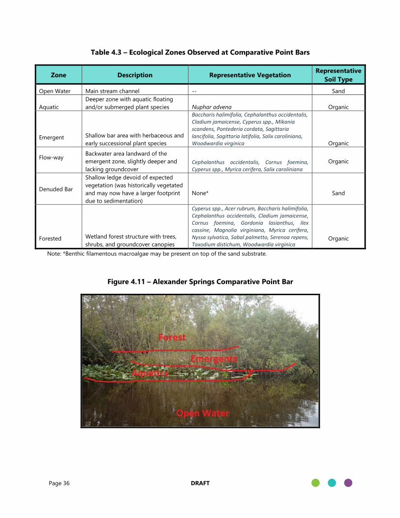
Page 36 DRAFT
Table 4.3 – Ecological Zones Observed at Comparative Point Bars
Zone Description Representative Vegetation Representative
Soil Type
Open Water Main stream channel -- Sand
Aquatic
Deeper zone with aquatic floating
and/or submerged plant species Nuphar advena Organic
Emergent Shallow bar area with herbaceous and
early successional plant species
Baccharis halimifolia, Cephalanthus occidentalis, Cladium jamaicense, Cyperus spp., Mikania scandens, Pontederia cordata, Sagittaria lancifolia, Sagittaria latifolia, Salix caroliniana, Woodwardia virginica Organic
Flow-way Backwater area landward of the
emergent zone, slightly deeper and
lacking groundcover
Cephalanthus occidentalis, Cornus foemina, Cyperus spp., Myrica cerifera, Salix caroliniana
Organic
Denuded Bar
Shallow ledge devoid of expected
vegetation (was historically vegetated
and may now have a larger footprint
due to sedimentation)
None* Sand
Forested Wetland forest structure with trees,
shrubs, and groundcover canopies
Cyperus spp., Acer rubrum, Baccharis halimifolia, Cephalanthus occidentalis, Cladium jamaicense, Cornus foemina, Gordonia lasianthus, Ilex cassine, Magnolia virginiana, Myrica cerifera, Nyssa sylvatica, Sabal palmetto, Serenoa repens, Taxodium distichum, Woodwardia virginica
Organic
Note: *Benthic filamentous macroalgae may be present on top of the sand substrate.
Figure 4.11 – Alexander Springs Comparative Point Bar
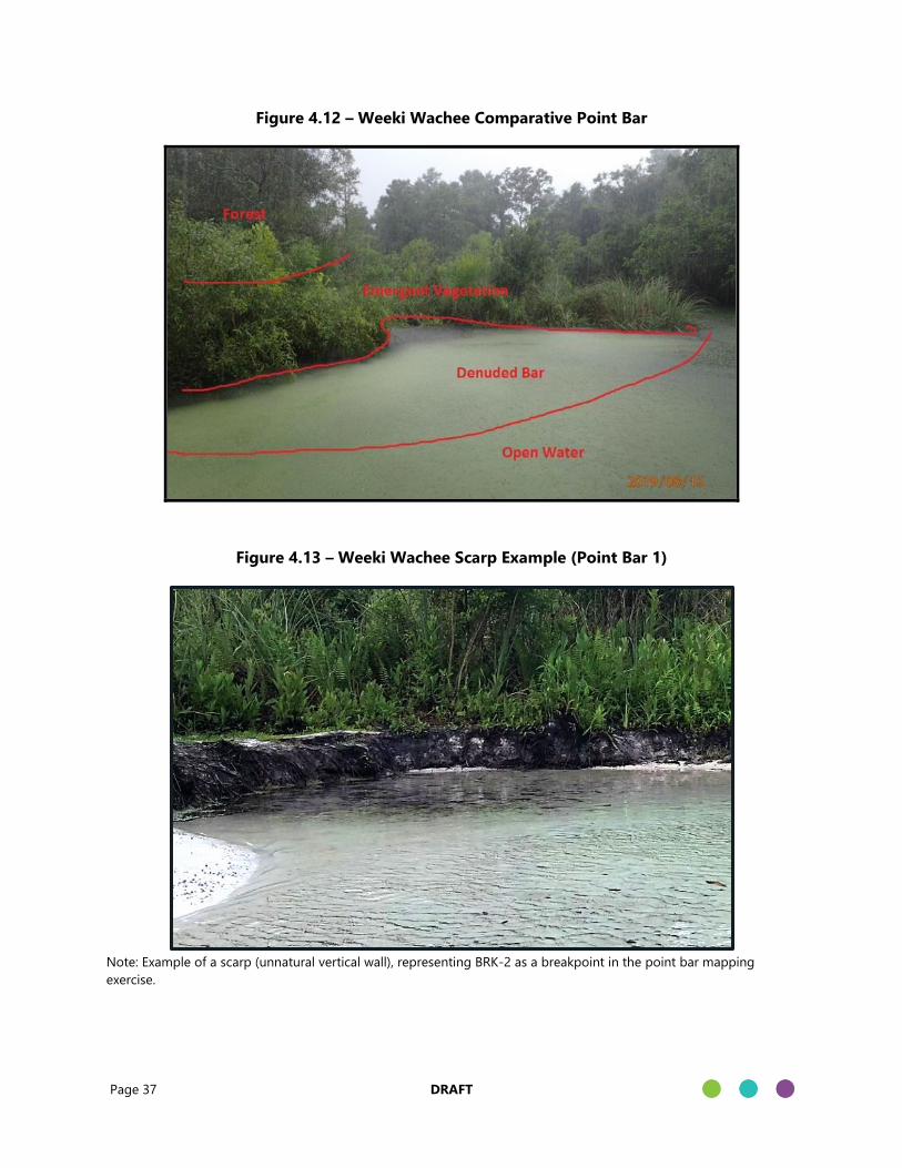
Page 37 DRAFT
Figure 4.12 – Weeki Wachee Comparative Point Bar
Figure 4.13 – Weeki Wachee Scarp Example (Point Bar 1)
Note: Example of a scarp (unnatural vertical wall), representing BRK-2 as a breakpoint in the point bar mapping
exercise.

Page 38 DRAFT
Figure 4.14 – Weeki Wachee Exposed Roots Example (Point Bar 33)
Of the 8 point bars mapped, 3 at Alexander Springs Run and 2 at Weeki Wachee River had an
emergent vegetation zone. The emergent zone at Alexander point bars averaged 61 feet long by
19 feet wide with an average area of 910 square feet, while the emergent zone at Weeki Wachee
point bars averaged 106 feet long by 23 feet wide with an average area of 2043 square feet (Table
4.4). Note that the emergent zone for the Weeki Wachee River appears to be substantially larger
because one of the point bars (#1/WW2) has a very large (although much impacted) emergent
zone. By comparison, the denuded point bars observed in the Weeki Wachee River averaged 72
feet long by 12 feet wide with an average area of 779 square feet. What is now denuded at the
Weeki Wachee River was likely once intact with vegetation and organic soils based on both the
comparable site point bar mapping results and the vegetation losses observable over time on
aerial photographs of the Weeki Wachee River.
At both Alexander Springs Run and Weeki Wachee River, the emergent zone contained organic
soils ranging from 0.2 to 3 feet thick, while the denuded zones at Weeki Wachee were just sand.
The average depth of the emergent zone relative to the bankfull stage was 1.7 feet at Alexander
Springs Run. The average depth of the waterward edge of the denuded bar at Weeki Wachee
(BRK1, which presented itself as a sand ledge) was 1.9 feet, while the average depth of the
landward edge of the denuded bar where the scarp occurred (BRK2) was 1.1 feet, indicating that
the current edge of the point bar at Weeki Wachee has a similar bankfull depth to the intact point
bars at Alexander Springs Run.

Page 39 DRAFT
Table 4.4 – Summary of Comparative Site Assessment Point Bar Dimensions
Site Zone Length
(ft)
Average
Width (ft)
Area (sq.
ft)
*Average
Depth Relative
to Bankfull (ft)
Organic
Soil
Thickness
(ft)
Average
Estimated
Organic Soil
(cy)
Alexander
Spring Run
Emergents
(n=3)
61
(48-71)
19
(16-22)
910
(726-1213)
1.7
(1.5-1.8) 0.5 - 3 57
Weeki
Wachee
River
Emergents
(n=2)
106
(20-191)
23
(8-38)
2043
(156-3930)
0.1
(0.1-0.2) 0.2 - 3 34
Denuded
(n=4)
72
(49-99)
12
(9-16)
779
(325-1204)
BRK1 Sand
Ledge:
1.9
(1.3-2.4)
BRK2 Scarp Toe:
1.1
(0.9-1.3)
Sand only -31
Note: Top number is the average, parentheses include the range (minimum-maximum).
*Average depth relative to bankfull indicates the relative elevation of the soil surface.
Using the mapped areas of point bar zones and the depth of organic soils in each zone, an
estimated volume of organic soils at each bar was calculated for Alexander Springs Run and Weeki
Wachee River. The emergent vegetation zones of Alexander Springs point bars were compared to
the emergent vegetation and denuded point bar zones of Weeki Wachee (inferring from historic
aerial interpretation that denuded point bars historically contained vegetation). Averaging organic
volumes at each site, Alexander Springs emergent zones characteristically contained 57 cubic
yards of organic soils per bar, Weeki Wachee emergent zones contained an average of 34 cubic
yards of organic soils per bar, and Weeki Wachee denuded zones are estimated to have lost an
average of 31 cubic yards per bar, when multiplying the area by the depth of soil loss (Table 4.4).
Denuded zone organic soil loss was estimated by multiplying the average zone area by the
average scarp depth.
4.4. Cumulative Assessment
4.4.1 Methodology
A cumulative assessment was conducted to document organic soil and vegetation losses at Weeki
Wachee River point bars by measuring apparent denudation surface areas and soil loss
thicknesses at 10 randomly selected point bars from the State Park to Rogers Park. The random
selection included at least two point bars in each functional process zone, at least one of which
was forested and one of which was herbaceous (locations in Map 4). General dimensions (length,
width, depth), soil, and vegetation data were recorded within each ecological zone at the 10
selected point bars. The data gathered in this assessment, as well data collected at reference point
bars in the comparative study, were then used to estimate soil and vegetation losses at denuded

Page 40 DRAFT
point bars, and to gain an understanding of the average conditions of the point bars along the
Weeki Wachee River. Detailed information including photographs, measurements, and soil and
vegetation data for each cumulative assessment point bar are provided in Appendix F.
Of the 10 point bars assessed on the Weeki Wachee River, 9 exhibited a denuded zone with scarps
and soil loss that appear to be from recreational use, while 1 remained largely intact. It should be
noted that at point bars classified as forested, it was unclear whether emergent herbaceous
vegetation zones had been lost or if the dense canopy had never provided conditions to support
emergent vegetation. It is also worth noting that similarly dense forested areas of Alexander
Springs Run did support emergent, herbaceous vegetation zones. Therefore, the assumption
would be that the forested bars on Weeki Wachee River should also have an herbaceous emergent
zone to be considered intact and unimpacted. The denuded zones measured at the cumulative
assessment point bars averaged 74 feet long and 13 feet wide, with an average area of 1,038
square feet and an average scarp thickness of 1.4 feet (Table 4.5).
To estimate the amount of organic soil lost at each denuded cumulative assessment site, each
site’s average scarp thickness was multiplied by the area of the denuded zone. Using this
approach, it can be estimated that nearly 500 cubic yards of organic soil has been lost from the
measured cumulative assessment point bars across over 9,300 square feet of measured denuded
zone (Table 4.5). Reference bar soil thicknesses were also considered for use to estimate soil
thickness loss at denuded bars. However, organic soil depths within intact emergent zones at both
Alexander Springs Run and Weeki Wachee River ranged from less than 1 foot to over 3 feet
(Appendix E). Due to the wide range of organic soil depths encountered at these reference point
bars, the scarp thickness was assumed to be the most accurate depth for estimating organic soil
losses at each particular point bar; however, using scarp thickness is a forensic estimate of actual
organic soil loss with degree of uncertainty regarding if it is an over- or under-estimation.
Table 4.5 – Summary of Cumulative Assessment Denuded Point Bar Dimensions (n=9)
Summary Statistic Length (ft) Average
Width (ft)
Area
(sq. ft)
Average
Scarp
Thickness
(ft)
Estimated
Organic Soil
Volume Loss
(cy)
Minimum 49 3 134 0.9 9
Maximum 116 26 2575 1.8 149
Average 74 13 1038 1.4 55
Total 670 -- 9338 -- 498
Note: Area displayed in table is not equal to length*width in table. Area of each point bar was calculated with bar’s
individual length and average width, but table shows minimum, maximum, and average dimensions across all bars.
In addition to the detailed assessment of the 10 selected point bars described above, locations
and estimated dimensions of an additional 24 bars with scarps that appeared to be from
recreational use were documented along the river (Map 4). The goal of this additional data
collection was to obtain more comprehensive information to help estimate total organic soil losses

Page 41 DRAFT
along the river. It should be noted that this additional assessment was conducted with rough
measurements, not measured with the more detailed methods described above in earlier sections.
The measurements and calculations were intended to provide a general estimate of total soil
volume loss along the length of the river.
The length of each scarp was estimated, and the thickness of each scarp was measured at one
representative location along the scarp. The 24 additional bars with scarped areas averaged 37
feet long and 1.1 feet thick (Table 4.6). To estimate the amount of organic soil lost at each
additional scarp, each site’s average scarp thickness was multiplied by the estimated length and
by the average width of the cumulative assessment sites’ denuded zone (13 feet). Using this
approach, it was estimated that nearly 500 cubic yards of organic soil has been lost from these
additional scarps (Table 4.6). Using the estimated lengths and the average 13-foot width, the
additional scarps have an associated denuded zone area of approximately 12,000 square feet.
Table 4.6 – Summary of Additional Observed Scarp Dimensions (n=24)
Parameter Length (ft) Scarp Thickness
(ft)
Estimated Organic
Soil Loss (cy)
Minimum 15 0.8 7
Maximum 110 2.0 51
Average 37 1.1 20
Total 880 -- 485
Totaling the estimated organic soil losses from the cumulative assessment sites and the additional
scarp sites, approximately 1,000 cubic yards of organic soil has been lost from point bars within
the Weeki Wachee River study area. Denuded zone surface area totals over 20,000 square feet,
which may be an indication of how much vegetation has been lost. As demonstrated in the
trample study, once vegetation has been trampled and lost, the denuded point bar no longer
holds organic soils. These soils wash away, exposing the sand below, which then becomes easily
transportable and is redistributed, causing downstream point bar dimensions to shift over time.
Due to these shifts, the apparent denuded zones measured in this study may be smaller or larger
in size than the actual footprint of vegetation and soil losses that have occurred over time.
Irrespective of the quantitative accuracy of the amount of soil involved, it is clear that the Weeki
Wachee River’s point bar equilibrium and ecological integrity has been severely compromised.
4.5. Inventory of Leaning Trees
While conducting cumulative assessments on Weeki Wachee River, it was noted that many trees
were leaning over or into the water at an angle that would make the trees susceptible to an
impending tree fall, particularly within FPZ-3. Many of the leaning trees had roots that appear to
have been exposed from soil washout/erosion and moderate to severe bank undercutting. Along
the spring run from the State Park to Rogers Park, 76 leaning trees were observed (56 in FPZ-3,

Page 42 DRAFT
26 in FPZ-2). Overall, the leaning trees appeared to be on outer bends of the river. At one outer
bend, at the Weeki Wachee Christian Camp, one large bay tree had fallen during the end of the
study, exposing the root system and disturbing the soils of the bank. Along the same outer bend
at the Christian Camp, several more leaning trees were noted along with approximately 6 feet of
bank undercutting (Figure 4.15). Bank undercutting increases potential for tree fall when trees
are rooted into the undercut bank, which can create a hazard and obstruction for navigation when
the tree falls into the river. Outer bends with severe undercutting can also be associated with point
bar enlargement, which appears to be occurring on several bars.
The Hernando County staff that maintain and remove fallen trees noted that many of the fallen
trees they remove used to be rope swing or jumping trees. Jumping trees and rope swings appear
to have multiple effects on point bar and bank morphology. The tree is a recreational draw,
attracting vessels to dock and users to wade and swim, which may expose shoreline to enhanced
vulnerability to scour and accelerated erosion of the banks. The energy transferred to the water
from the impact of individuals jumping from heights can produce additional erosive forces not
normal for the river in the form of waves. If enough soil is lost that the roots can no longer hold
the tree in place, it may fall, tearing soil up with the roots, and leaving exposed soils that can then
be washed downstream.
Figure 4.15 – Leaning Trees on Right Bank at Weeki Wachee Christian Camp
4.6. Desktop GIS Inventory
GIS software in conjunction with ground-truthing in the field were used to create an inventory of
features that provide recreational access to the river such as docks, boat ramps, seawalls, and
other (including earthen ramps, stairs, and cleared grass slopes (Table 4.7). Additionally, GIS was
used to assess the available parking spaces at the State Park and Rogers Park, along with any
other identifiable vendor parking areas (Table 4.8). All discernable vessel vendors (Table 4.9) were
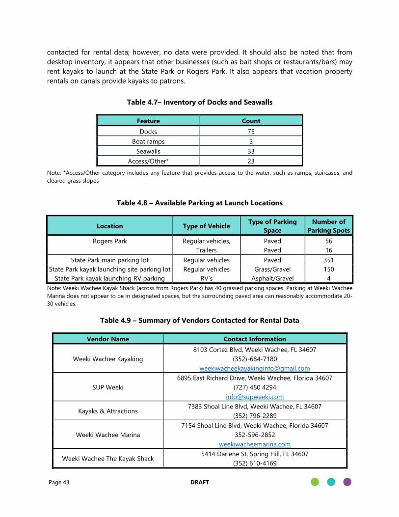
Page 43 DRAFT
contacted for rental data; however, no data were provided. It should also be noted that from
desktop inventory, it appears that other businesses (such as bait shops or restaurants/bars) may
rent kayaks to launch at the State Park or Rogers Park. It also appears that vacation property
rentals on canals provide kayaks to patrons.
Table 4.7– Inventory of Docks and Seawalls
Feature Count
Docks 75
Boat ramps 3
Seawalls 33
Access/Other* 23
Note: *Access/Other category includes any feature that provides access to the water, such as ramps, staircases, and
cleared grass slopes
Table 4.8 – Available Parking at Launch Locations
Location Type of Vehicle Type of Parking
Space
Number of
Parking Spots
Rogers Park Regular vehicles, Paved 56 Trailers Paved 16
State Park main parking lot Regular vehicles Paved 351
State Park kayak launching site parking lot Regular vehicles Grass/Gravel 150
State Park kayak launching RV parking RV’s Asphalt/Gravel 4
Note: Weeki Wachee Kayak Shack (across from Rogers Park) has 40 grassed parking spaces. Parking at Weeki Wachee
Marina does not appear to be in designated spaces, but the surrounding paved area can reasonably accommodate 20-
30 vehicles.
Table 4.9 – Summary of Vendors Contacted for Rental Data
Vendor Name Contact Information
Weeki Wachee Kayaking
8103 Cortez Blvd, Weeki Wachee, FL 34607
(352)-684-7180
SUP Weeki
6895 East Richard Drive, Weeki Wachee, Florida 34607
(727) 480 4294
Kayaks & Attractions 7383 Shoal Line Blvd, Weeki Wachee, FL 34607
(352) 796-2289
Weeki Wachee Marina
7154 Shoal Line Blvd, Weeki Wachee, Florida 34607
352-596-2852
weekiwacheemarina.com
Weeki Wachee The Kayak Shack 5414 Darlene St, Spring Hill, FL 34607
(352) 610-4169
Page 44 DRAFT
4.7. Summary of Fluvial Geomorphology Assessment
From interpretation of aerial imagery, it is apparent that point bars along the Weeki Wachee River
have lost vegetation and organic soils since 2008 (the oldest available clear aerial imagery). An
experimental study of recreational trampling showed that even a small amount of trampling can
impact vegetation and cause organic soil losses, and that trampling increases turbidity, especially
when it occurs in organic soils. The trampling study also showed that vegetation on the
submerged edges of point bars are the most likely to be extensively impacted.
The less-impacted comparison sites at Alexander Springs Run showed that point bars, even in
densely forested reaches, support emergent herbaceous vegetation and contain organic
substrates, while point bars surveyed at the Weeki Wachee River had a denuded zone devoid of
emergent vegetation or the emergent zone was truncated. The comparative study results
provided another layer of evidence and documented that point bars in Weeki Wachee River have
been impacted in comparison to Alexander Spring Run and approximately 30 cy/bar has been lost
from Weeki Wachee River point bars.
The cumulative assessment showed that 9 out of 10 point bars on the Weeki Wachee River were
impacted and had denuded herbaceous zones, with only 1 out of 10 assessed bars remaining
intact. In addition, 33 point bars showed that approximately 1-2 ft of organic soil depth has been
lost at many point bars on the river along with up to 20,000 square feet of estimated vegetation
loss based on the sizes of the denuded zones observed. The denudation on this set of bars likely
resulted in something on the order of 1,000 cubic yards of organic soil alone (approximately 60
dump truck loads).
Page 45 DRAFT
STATISTICAL ANALYSIS TO ASSESS RECREATIONAL IMPACTS
The historic aerials, physical assessments, and experiments detailed in previous sections
consistently suggest that recreation has impacted the vegetation, soils, and morphology of the
river. Experimental turbidity recordings before and after trampling showed that trampling leads
to increases in turbidity. The data collected as part of this project were analyzed, along with other
environmental data to determine if statistically significant relationships exist between recreation
and water quality parameters, specifically turbidity. Turbidity is caused by light scatter from fine
particles floating in the water and a variety of activities can increase the load of such particles,
including trampling, docking, wave induction, and prop wash from motor boats. Increased
turbidity reduces water clarity and light penetration through the water column, which can affect
the photosynthesis of submerged aquatic plant communities. Increased turbidity may also
indicate suspension of sediments that may redeposit and smother aquatic plants and other
benthic habitats. Florida spring runs characteristically have very low turbidity, so elevated turbidity
indicates potential water quality issues related to recreational activity if it can be measured to
increase during such activities.
Wood concurrently sampled turbidity, total suspended solids (TSS), and volatile suspended solids
(VSS) at varying levels of recreational use to statistically assess associations between these
variables. All three variables essentially measure the amount of suspended particles in the water
column and are typically co-variates when the variables are used as proxies for water clarity,
quality, and to assess potential sediment transport. However, during quality control processing
and screening (i.e. review of laboratory qualifier codes and other reported quality controls), the
TSS and VSS data were found to be below detection and were not used for statistical analyses.
The processed and screened turbidity dataset was found to be adequate for statistical analyses
and were used for several different statistical tests as described below. It should be noted that
because turbidity can increase absent recreational influence in response to rainfall, and due to
algal production as the day unfolds, Wood accounted for such responses in the statistical
assessments.
5.1. Exploratory Analysis with Long-Term Data
5.1.1 Turbidity Trend Analysis
Trend analysis was performed on the quarterly average time series of SWFWMD ambient turbidity
data from stations 20923 (SWFWMD WW1, Wood WW2), 20600 (SWFWMD WW3, near Wood
WW3), and 20650 (SWFWMD WW5, between Wood WW4 and Rogers Park) using the USGS
Fortran code for the nonparametric Seasonal Kendall Test, which acknowledges and adjusts for
potential autocorrelation (Helsel et al. 2006). The trend analysis was performed on time series with
and without outliers (defined as greater than 2*standard deviation). Overall, the results showed
significant increasing trends at all stations from 2006 to 2019 (except for station 20600 with
outliers.) The complete trend analysis results are shown in Table 5.1.
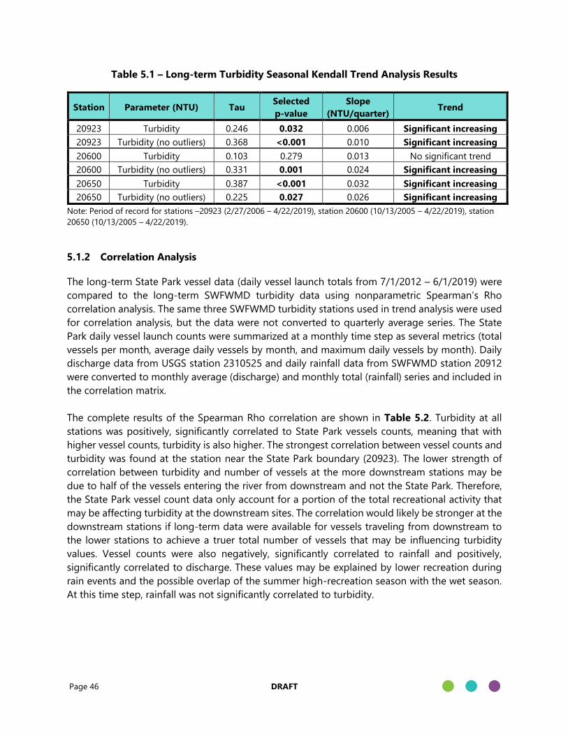
Page 46 DRAFT
Table 5.1 – Long-term Turbidity Seasonal Kendall Trend Analysis Results
Station Parameter (NTU) Tau Selected
p-value
Slope
(NTU/quarter) Trend
20923 Turbidity 0.246 0.032 0.006 Significant increasing
20923 Turbidity (no outliers) 0.368 <0.001 0.010 Significant increasing
20600 Turbidity 0.103 0.279 0.013 No significant trend
20600 Turbidity (no outliers) 0.331 0.001 0.024 Significant increasing
20650 Turbidity 0.387 <0.001 0.032 Significant increasing
20650 Turbidity (no outliers) 0.225 0.027 0.026 Significant increasing
Note: Period of record for stations –20923 (2/27/2006 – 4/22/2019), station 20600 (10/13/2005 – 4/22/2019), station
20650 (10/13/2005 – 4/22/2019).
5.1.2 Correlation Analysis
The long-term State Park vessel data (daily vessel launch totals from 7/1/2012 – 6/1/2019) were
compared to the long-term SWFWMD turbidity data using nonparametric Spearman’s Rho
correlation analysis. The same three SWFWMD turbidity stations used in trend analysis were used
for correlation analysis, but the data were not converted to quarterly average series. The State
Park daily vessel launch counts were summarized at a monthly time step as several metrics (total
vessels per month, average daily vessels by month, and maximum daily vessels by month). Daily
discharge data from USGS station 2310525 and daily rainfall data from SWFWMD station 20912
were converted to monthly average (discharge) and monthly total (rainfall) series and included in
the correlation matrix.
The complete results of the Spearman Rho correlation are shown in Table 5.2. Turbidity at all
stations was positively, significantly correlated to State Park vessels counts, meaning that with
higher vessel counts, turbidity is also higher. The strongest correlation between vessel counts and
turbidity was found at the station near the State Park boundary (20923). The lower strength of
correlation between turbidity and number of vessels at the more downstream stations may be
due to half of the vessels entering the river from downstream and not the State Park. Therefore,
the State Park vessel count data only account for a portion of the total recreational activity that
may be affecting turbidity at the downstream sites. The correlation would likely be stronger at the
downstream stations if long-term data were available for vessels traveling from downstream to
the lower stations to achieve a truer total number of vessels that may be influencing turbidity
values. Vessel counts were also negatively, significantly correlated to rainfall and positively,
significantly correlated to discharge. These values may be explained by lower recreation during
rain events and the possible overlap of the summer high-recreation season with the wet season.
At this time step, rainfall was not significantly correlated to turbidity.

Page 47 DRAFT
Table 5.2 – Results of Spearman Rho Correlation Analysis
Turbidity at
20923
Turbidity at
20600
Turbidity at
20650
Monthly Total
Vessels
Avg Daily
Vessels
(by month)
Turbidity at 20923 0.581
0.001
Turbidity at 20650 0.322 0.348
0.094 0.069
Monthly Total Vessels 0.588 0.374 0.365
0.001 0.05 0.056
Avg Daily Vessels (by
month)
0.559 0.356 0.374 0.998
0.002 0.063 0.05 0
Max Daily Vessels (by
month)
0.518 0.294 0.163 0.881 0.872
0.005 0.129 0.408 0 0
Discharge 0.205 0.203 0.312 0.426 0.436
0.295 0.3 0.106 0.024 0.02
Rainfall -0.047 -0.251 -0.257 -0.479 -0.497
0.81 0.197 0.186 0.01 0.007
Note: The top value in cell is Spearman's Rho, bottom is p-value. Bold p-values indicate statistical significance at
alpha=0.05. Bold italic p-values indicate statistical significance at alpha=0.1. Green shading indicates positive, significant
correlation. Red shading indicates negative, significant correlation.
5.2. Statistical Analyses with Field, Camera, and Sonde Data
The exploratory analysis with long-term data showed a correlation between number of vessels
launched from the State Park and turbidity, so the relationship was further explored in more detail
and with a tighter sampling frequency using data collected as part of this study (details regarding
data collection intervals and protocols are provided in Section 2). Two independently collected
datasets were used to identify if relationships exist between turbidity and recreational use in the
river at Wood’s monitoring stations:
• Continuous turbidity (FNU) data were collected in situ via a sonde instrument (deployed
and retrieved by FDEP). Concurrent continuous recreational use data recorded by video
cameras (deployed and retrieved by Wood) was transcribed by SWFWMD from recorded
video footage. This coupled dataset is referred to as the ‘continuous dataset.’
• On the 9 sampling events conducted by Wood, grab samples were collected in the field
and analyzed in the FDEP laboratory for turbidity (NTU). Concurrent recreational use data
(user and vessel counts) were collected in the field by Wood. This dataset is referred to as
the ‘grab-sample dataset.’
Each of the datasets listed above also included daily rainfall and spring discharge (flow) data
recorded at SWFWMD station 20912 and USGS station 2310525, respectively (same data as used
in correlation analysis).

Page 48 DRAFT
The statistical analyses treated turbidity as the response variable. As is common for water quality
data, the turbidity data were log-normally distributed. Therefore, to meet assumptions for the
applicable parametric and linear analyses, the turbidity data were log10 transformed prior to
analysis. The results should be interpreted in terms of explanatory variables’ influence on the
order of magnitude of turbidity, and not simply on the absolute value.7
Explanatory variables in each analysis included the sampling site (spatial variation), seasonal and
daily effects (temporal variation), user counts, vessel counts, rainfall (in.), and spring discharge
(cfs). User counts, vessel counts, and rainfall were broken out into several variables (‘predictors’)
used in the statistical models (Table 5.3). Based on the raw count data, various hourly and
cumulative user and vessel counts were developed: the number of users present during the one
hour prior to sampling (e.g., hourly users, user.hour) and the running count of users up until the
sampling time each day (e.g., hourly cumulative users, user.cumu).
Table 5.3 – Summary of Variables used in Analyses
Variable Name Description Unit Type
turb.ntu turbidity analyzed in lab (grab sample) NTU continuous
turb.fnu turbidity recorded by sonde FNU continuous
site turbidity sampling site (WW1, WW2, WW3, or WW4) categorical
date turbidity sampling date categorical
time turbidity sampling time categorical
rain.in.d0 rainfall on sampling date in continuous
rain.in.d1 rainfall one day prior to sampling date in continuous
rain.in.d2 rainfall two days prior to sampling date in continuous
rain.in.d3 rainfall three days prior to sampling date in continuous
rain.in.tot total rainfall during sampling date and the three days prior in continuous
flow.cfs spring discharge cfs continuous
user.hour count of users during the one hour prior to sampling time discrete
user.cumu cumulative count of users on the sampling date, up until the
sampling time discrete
swim.hour count of people wading/swimming during the one hour prior
to sampling time discrete
swim.cumu cumulative count of people wading/swimming on the
sampling date, up until the sampling time discrete
vessTOT.hour count of vessels (all types) during the one hour prior to
sampling time discrete
vessTOT.cumu cumulative count of vessels (all types) on the sampling date,
up until the sampling time discrete
dockTOT.hour count of docked vessels (all types) during the one hour prior
to sampling time discrete
7 The log transformation replaces each observed turbidity value with the base-10 logarithm of that value: The logarithm function returns the exponent to which 10 must be raised to produce the original value. For instance, the logarithm of 10 is 1, and the logarithm of 100 is 2, because 101=10 and 102=100. Therefore, an increase of one on the logarithmic scale represents a tenfold increase in turbidity.
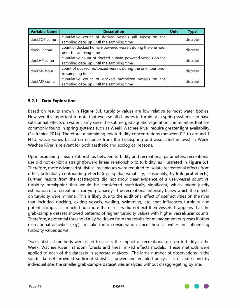
Page 49 DRAFT
Variable Name Description Unit Type
dockTOT.cumu cumulative count of docked vessels (all types) on the
sampling date, up until the sampling time discrete
dockHP.hour count of docked human-powered vessels during the one hour
prior to sampling time discrete
dockHP.cumu cumulative count of docked human-powered vessels on the
sampling date, up until the sampling time discrete
dockMP.hour count of docked motorized vessels during the one hour prior
to sampling time discrete
dockMP.cumu cumulative count of docked motorized vessels on the
sampling date, up until the sampling time discrete
5.2.1 Data Exploration
Based on results shown in Figure 5.1, turbidity values are low relative to most water bodies.
However, it’s important to note that even small changes in turbidity in spring systems can have
substantial effects on water clarity since the submerged aquatic vegetation communities that are
commonly found in spring systems such as Weeki Wachee River require greater light availability
(Szafraniec 2014). Therefore, maintaining low turbidity concentrations (between 0.2 to around 1
NTU, which varies based on distance from the headspring and associated inflows) in Weeki
Wachee River is relevant for both aesthetic and ecological reasons.
Upon examining linear relationships between turbidity and recreational parameters, recreational
use did not exhibit a straightforward linear relationship to turbidity, as illustrated in Figure 5.1.
Therefore, more advanced statistical techniques were required to isolate recreational effects from
other, potentially confounding effects (e.g., spatial variability, seasonality, hydrological effects).
Further, results from the scatterplots did not show clear evidence of a user/vessel count vs.
turbidity breakpoint that would be considered statistically significant, which might justify
estimation of a recreational carrying capacity—the recreational intensity below which the effects
on turbidity were minimal. This is likely due to the additional effect of user activities on the river
that included docking, exiting vessels, wading, swimming, etc. that influences turbidity and
potential impact as much if not more than if users did not exit their vessels. It appears that the
grab-sample dataset showed patterns of higher turbidity values with higher vessel/user counts.
Therefore, a potential threshold may be drawn from the results for management purposes if other
recreational activities (e.g.) are taken into consideration since these activities are influencing
turbidity values as well.
Two statistical methods were used to assess the impact of recreational use on turbidity in the
Weeki Wachee River: random forests and linear mixed effects models. These methods were
applied to each of the datasets in separate analyses. The large number of observations in the
sonde dataset provided sufficient statistical power and enabled analysis across sites and by
individual site; the smaller grab-sample dataset was analyzed without disaggregating by site.

Page 50 DRAFT
Figure 5.1 – Scatterplots of Turbidity vs. Hourly User and Vessel Counts
Note: The top two figures depict the continuous dataset, and the bottom two depict the grab-sample dataset. The y-
axes are hourly turbidity on a logarithmic scale.
5.2.2 Random Forest Methodology
Using R package ‘gbm’ (Greenwell et al. 2019; R Core Team 2018), random forests with gradient
boosting were applied to rank predictors according to their ‘relative influence’ on turbidity. A
random forest model develops an ensemble of ‘decision trees’ that each partition the predictor
space using random subsets of predictors; while each tree is a weak predictor, the collective
prediction skill of the ensemble is generally much greater (James et al. 2013). Gradient boosting
improves prediction skill by sequentially fitting trees to the residuals from previous trees. Cross-
validation, which is training the model on random subsets of data (‘training data’) and testing the
model on each out-of-sample data set (‘test data’), was applied to optimize tuning parameters
that control the algorithm (the loss function and the number of sequential trees in each model).

Page 51 DRAFT
The boosted random forest model provides a relative influence metric that reflects each predictor’s
contribution to improved prediction skill across the ensemble (Ridgeway 2019).
Modeling with random forests offers increased ability to detect complex, nonlinear relationships
between predictors and the response, and typically increases out-of-sample prediction skill as
compared to classical regression. However, these advantages come with a trade-off: The random
forests’ results are less interpretable, and inferences about predictor-response relationships are
limited to the relative-influence ranking. This is in contrast to least-squares regression, which
quantifies the relationships with a coefficient estimate for each predictor. Consequently, results
from the random forest models are presented only as a preliminary indicator of the variables with
the greatest influence on turbidity. The results gain credibility to the extent that cross-validation
demonstrates skillful prediction on out-of-sample data.
The out-of-sample prediction skill of each model was measured using Nash-Sutcliffe efficiency
(NSE):
𝑁𝑆𝐸 = 1 − ∑ (�̂�𝑖 − 𝑦𝑖)2𝑛
𝑖=1
∑ (𝑦𝑖 − �̅�)2𝑛𝑖=1
= 1 − (𝑅𝑀𝑆𝐸
𝜎)
2
where yi and ŷi are the ith observed and predicted values of the response variable, respectively; ȳ
was the mean of the observed response values. Equivalently, the NSE can be expressed in terms
of the ratio between the root-mean-squared error (RMSE) of the model and the standard
deviation (σ) of the response data, as above. A value of NSE=0 indicates that the model predicts
the mean response value; values below zero indicate that the mean is a better predictor than the
model; values above zero indicate that the model is a better predictor than the mean; and a value
of NSE=1 indicates a perfect fit between the predicted and observed response values. A minimum
threshold of NSE≥0.50 was adopted as an acceptance criterion for the prediction skill of each
model (Moriasi et al. 2007). Next, the random forest results were used to inform specification of
linear mixed effects models that tested the identified predictor-turbidity relationships for
statistical significance.
5.2.3 Linear Mixed Effects Model Methodology
A linear mixed effect model (LMEM) is a generalized form of least-squares regression that
estimates coefficients for fixed effects (measured variability in the explanatory variables) and their
statistical significance, while controlling for random effects—unmeasured variability attributed to
spatial or temporal replication (Galecki and Burzykowski 2013).
Ordinary least-squares regression estimates response values according to the equation
ŷ = Xβ
where ŷ is the n×1 vector containing predicted values of the response variable (e.g., turbidity); X
is the n×(p+1) design matrix, whose first column is a vector of 1’s and whose subsequent p
columns each contain n observed values of a predictor; and β is the (p+1)×1 coefficient vector
[β0, β1, β2, …, βp]T, whose first element is the estimated intercept and whose subsequent elements
are the slopes estimated for p predictors. The intercept represents the baseline value of the

Page 52 DRAFT
response (given no influence from the predictors), and each slope represents the estimated
adjustment to the mean response value given a unit change in a predictor.
A linear mixed effects model adds a term to the above regression equation to estimate intercepts
(and optionally, slopes) for random effects:
ŷ = Xβ + Zα
where X is the design matrix for fixed effects; β is the fixed-effects coefficient vector; Z is the
design matrix for random effects; and α is the random-effects coefficient vector (Galecki and
Burzykowski 2013). The α vector may include random intercepts and slopes, or random intercepts
only. Each random intercept represents an adjustment to the baseline intercept β0, based on
membership of an observation in a random-effects group. For instance, a random intercept for
each sampling site would adjust the baseline turbidity values for each site (assuming no influence
from the fixed-effects predictors).
The R package ‘nlme’ was used to develop the mixed effects models (Pinheiro et al. 2018; R Core
Team, 2018). Specification of each LMEM was informed by the results from the corresponding
random forest model. The LMEMs tested whether the five top-ranked predictors identified by
each random forest model were statistically significant (alpha=0.05) predictors of turbidity (log-
transformed), while controlling for spatial and temporal variability as random effects. Akaike’s
Information Criterion (AIC) was applied to select the variables for inclusion as random effects (from
among sampling site, date, and time, as applicable, Akaike 1973). The AIC balances goodness of
fit with model complexity (the number of parameters in the model) to select the most efficient
model from a set of candidate models.
For each mixed-effects model, the Pearson residuals were examined to ensure that the residuals
were unstructured with respect to fitted values, fixed effects values, and random effects values.
Further, the prediction skill of each model using the NSE metric was computed (see the previous
section). Here, NSE is equivalent to the familiar coefficient of determination R2, in that it reflects
the amount of variance from the mean explained by the model. The NSE values reported for
mixed-effects models were computed using the full set of turbidity data and predictions. The p-
values are reported for fixed effects as provided by the lme() function in the ‘nlme’ package: the
function computes p-values after estimating the degrees of freedom as n–p, where n is the sample
size and p is the number of parameters in the model.

Page 53 DRAFT
5.2.4 Results of Random Forest Models
Random forest models were run to identify the variables exerting the greatest ‘relative influence’
on turbidity across all four sites and at each site individually. In addition, the random forest results
informed the selection of variables for hypothesis testing with mixed effects models (discussed in
following section). The predictors considered by each model included user counts, vessel counts,
rainfall, and spring discharge, as well as the sampling site, date, and time (full list of variables in
Table 5.3). Each model yielded an acceptable fit to out-of-sample data during cross-validation
(NSE>0.50), suggesting reliability for drawing inferences (Table 5.4).
Overall, the analysis sought to identify recreational factors influencing turbidity while controlling
for the spatial and temporal variability associated with the sampling sites, dates, and times. These
categorical variables were therefore included in the random forest models although they were not
of primary interest as predictors of turbidity. Because sampling site, date, and time ranked highly
in each model, they were specified as candidate ‘random effects’ in the mixed effects models
(following section).
The top-five numerical predictors in each random forest model are marked in Table 5.4. Among
the five models, the hourly cumulative vessel count (vessTOT.cumu) most often ranked highest.
The hourly cumulative counts of users (user.cumu) and people wading/swimming (swim.cumu)
were also highly ranked across models. These results provide a preliminary indication that both
the cumulative number of vessels per hour and the cumulative number of users in the water per
hour each day exerted a relatively strong influence on turbidity concentrations.
Spring discharge (flow.cfs) was ranked as the most influential predictor of turbidity by the WW3
model (continuous sonde data). Otherwise, the random forest models detected zero influence on
turbidity from rainfall and spring discharge. These results should not be interpreted as evidence
that rainfall and spring discharge did not physically influence turbidity. Instead, the results may
be an artifact of the temporal resolution of these data. The daily resolution of the rainfall and
discharge data means that their (numerical) variability would easily be captured by the categorical
sampling date variable (date).
The motorized vessel counts (dockMP.hour and dockMP.cumu) did not rank in the top-five most
influential predictors across models. This result should not be interpreted as evidence that
motorized vessels did not influence turbidity. Instead, the result likely reflects the low variance in
the motorized vessel data, relative to the variance present in other predictors.

Page 54 DRAFT
Table 5.4 – Summary of Random Forest Model Results
Dataset Continuous Sonde and Camera Count Data Grab-Sample and Field
Count Data
Response variable Turbidity (log10, FNU) Turbidity (log10, NTU)
Site WW1 WW2 WW3 WW4 All sites All sites
Observations n 384 480 433 362 1659 144
Error Statistics test NSE 0.801 0.933 0.966 0.539 0.562 0.609
test RMSE 0.435 0.297 0.273 0.295 0.746
Predictor
rain.in.d0
rain.in.d1
rain.in.d2
rain.in.d3
rain.in.tot
flow.cfs X
vessTOT.hour x
vessTOT.cumu X X X X
user.hour x x
user.cumu x x x x x
dockHP.hour x
dockHP.cumu x x x
dockMP.hour
dockMP.cumu
dockTOT.hour
dockTOT.cum
u x
x
swim.hour x X x
swim.cumu x x x x
Note: The top-five predictors from each model are marked; a bold X indicates the top-ranked predictor. (The models
for WW1 and all sites based on the continuous sonde data identified only three numerical variables with non-zero
influence.) Error statistics on out-of-sample (‘test’) data indicate that the models provide a reliable basis for inference.
5.2.5 Results of Linear Mixed Effects Models
Based on the random forest model results, linear mixed effects models were specified to test
whether various user and vessel counts had statistically significant effects on turbidity, after
controlling for spatial and temporal variability arising from replicate sampling.
Each selected predictor was correlated with each other predictor (shown in Appendix G).
Including correlated predictors (i.e. co-variates) in the same model would make coefficient
estimation and hypothesis testing unreliable, because the regression procedure would be unable
to accurately isolate the effect of each correlated variable on the response variable (turbidity). To
avoid this problem, a separate mixed-effects model (and hypothesis test) was developed for each
selected predictor.
AIC was applied to select the variables for inclusion as random intercepts for each LMEM; random
slopes were not included. For the LMEM of the grab-sample dataset (all sites), random intercepts
were specified by site, date, and time. For the continuous sonde dataset (all sites), random
intercepts were specified by site and date (inclusion of random intercepts for time did not improve
Page 55 DRAFT
the AIC score). Likewise, for each of the 4 site-specific models (continuous sonde dataset), random
intercepts were specified by date.
Each mixed-effects model achieved a high NSE value (NSE≥0.85), and visual checks of each
model’s Pearson residuals did not show evidence of residual structure or autocorrelation. Results
of the hypothesis tests are summarized in Table 5.5. Each of the statistically significant coefficient
estimates associated with user and vessel counts were positive, indicating a significantly positive
relationship with turbidity.
The following results are from analysis of the continuous sonde dataset. The mixed effects model
for all sites identified the hourly cumulative counts of docked human-powered vessels and people
wading/swimming as highly significant predictors of turbidity (p < 0.0001). Results from the site-
specific mixed effects models generally agreed with these results:
• At WW1, the hourly cumulative counts of vessels (all types) and users were identified as
significant predictors of turbidity (p=0.0002 and p=0.0003, respectively).
• At WW2, the hourly cumulative counts of vessels (all types), docked vessels (all types),
users, docked human-powered vessels, and people wading/swimming were identified as
significant predictors of turbidity (p < 0.0001).
• At WW3, spring discharge and the hourly cumulative counts of users, docked human-
powered vessels, and people wading/swimming were identified as significant predictors
of turbidity (p < 0.0001). The coefficient estimated for spring discharge (flow.cfs) was
negative, indicating a negative relationship between discharge and turbidity.
• At WW4, the cumulative hourly counts of vessels (all types), users, and docked human-
powered vessels were identified as significant predictors of turbidity (p < 0.0001). Also,
the hourly counts of people wading/swimming (p=0.0025) and users (p < 0.0001) were
identified as significant predictors of turbidity.
Several predictors identified as highly influential by a random forest model were not identified as
statistically significant by the LMEMs, which included the number of people wading/swimming in
the all-sites model (p=0.582), the hourly user count at WW1 (p=0.058), and the hourly count of
vessels at WW3 (p=0.31).
The mixed effects model for the grab-sample dataset identified the hourly cumulative counts for
vessels (all types), users, docked vessels (all types), and people wading/swimming as significant
predictors of turbidity (p < 0.0001), which essentially corroborated the results from the continuous
sonde dataset analysis. The hourly count of people wading/swimming was not identified as a
significant predictor (p=0.31).

Page 56 DRAFT
Table 5.5 – Summary of Hypothesis Test Results from Linear Mixed Effects Models
Dataset Continuous Sonde and Camera Count Data
Grab-Sample
and Field Count
Data
Response variable Turbidity (log10, FNU) Turbidity (log10,
NTU)
Site WW1 WW2 WW3 WW4 All sites All sites
Predictor
flow.cfs <0.01
vessTOT.hour 0.31
vessTOT.cumu <0.01 <0.01 <0.01 <0.01
user.hour 0.06 <0.01
user.cumu <0.01 <0.01 <0.01 <0.01 <0.01
dockHP.hour <0.01
dockHP.cumu <0.01 <0.01 <0.0001
dockMP.hour
dockMP.cumu
dockTOT.hour
dockTOT.cumu <0.01 <0.01
swim.hour 0.0025 0.58 0.31
swim.cumu <0.01 <0.01 <0.01 <0.01
Note: Each p-value represents the result from a model testing the significance of a single predictor (fixed effect) on the
turbidity response, after controlling for spatial and temporal variability (random effects). Values in bold indicate
statistical significance (α=0.05). All significant coefficient estimates are positive, except for flow.cfs (indicated by italics).
5.3. Summary of Statistical Analysis to Assess Recreational Impacts on Water Quality
The statistical analysis results provided empirical evidence that both the cumulative number of
vessels and users per hour contributed to turbidity along the spring run during the study period
(July 2018 through June 2019). Hypothesis tests using linear mixed effects models corroborated
the initial results from the random forest models. The fact that the models largely favored
cumulative user and vessel counts over hourly counts suggests that recreation has an additive and
cumulative effect on turbidity, and thus water clarity and quality. In summation, the results
suggest that there are statistically significant relationships between the number of users/vessels
and turbidity, and also between in-water recreational activities, such as docking, wading, and
swimming and turbidity in the Weeki Wachee River. These results also suggest that a simple
reduction in the number of users/vessels alone may not reduce the effects on turbidity and water
clarity/quality and the in-water activities will need to be considered before making important
management decisions on recreational use.

Page 57 DRAFT
MANAGEMENT OPTIONS
While this study did not seek to define specific values for the recreational carrying capacity of the
Weeki Wachee River, it did find links between recreational activities and ecological degradation
and collected a large, varied dataset which will be useful for guiding management decisions or
directing future focused studies. The data, analyses, and observations from this study have
informed a preliminary list of possible management options that have potential to reduce the
observed impacts from recreation.
Key observations include:
• Point bars started to be denuded of herbaceous vegetation between 2008 and 2011,
indicating user impacts commenced before censusing data was collected starting in 2012.
• By 2016, many points bars had become severely denuded of vegetation, and some were
accreting sandy sediments presumably from upstream erosion of the denuded bars. Stress
and erosion of the opposite streambanks from the accreting point bars became substantial
at some locations during our study in 2019.
• The period from 2012 to 2016 saw a linear increase in users, with a moderate decline to
current levels thereafter. There has been no apparent trend in point bar recovery during
the reduced use. In fact, point bars have continued to denude. A total of 20,000 square
feet of shoreline vegetation habitat has been lost.
• Denudation appears to be initiated by vessel docking dislodging organic soils and
vegetation on the point bars. This sets up a cascading series of events by facilitating more
foot traffic at the impacted areas, expanding the denudation. Once a sandy beach is
exposed, it contributes sand to the run that would otherwise not leave the bar. Organic
soil releases are estimated at about 30 cy/bar based on the comparative and cumulative
assessments, which sums up to approximately 1,000 cubic yards (approximately 60 dump
trucks) from 33 impacted point bars.
• Rope swings appear to generate additional vessel docking and wading, which may
accelerate impacts. Further, trees with rope swings and those used for climbing and
jumping have been observed to fall more rapidly than if not used for these purposes.
• Effects of trampling of vegetation and the underlying soil matrix were documented and
were shown to cause immediate and mid-term effects on recovery.
• Points bars release substantial turbidity from organic soil releases into the run when they
are initially being denuded, but less once the vegetation and organic soils have been rather
fully depleted of organic soils. If this study was conducted during a time prior to the point
bars being denuded, then the effects on turbidity from recreational use would have likely
been more pronounced. Thus, the turbidity increases that occurred during this study in
direct association with increased vessels and users would likely be much more substantial
if the river’s point bars were in better ecological condition.
Page 58 DRAFT
• A clear breakpoint between the number of users/vessels was not found that would be
useful for setting a carrying capacity simply on the number of users/vessels. However,
statistical analyses provided empirical evidence that cumulative number of vessels/users
and in-water activities such as docking, wading, and swimming contributed significantly
to turbidity along the river, which suggests that recreation has negative effects on water
quality. A potential threshold may be drawn from the results for management purposes
if in-water and on-bar recreational activities are taken into consideration since these
activities are influencing turbidity values.
• The sandy point bars at the Weeki Wachee River are a human activity artifact and are
unnatural perturbations for Florida spring runs in general and represent a state change for
the river that commenced sometime between 2008 and 2011.
• It appears that limits on the number of users launching from the State Park may have
reduced the number of vessels on the river. Partying on upstream point bars appeared to
decline once the disposables ban was enforced. However, even though partying may have
declined, the in-water and on-bar activities may still be causing impacts.
• Downstream access points from Rogers Park and other sites contribute up to 50% of users
for the lower point bars, but less for upstream point bars. This suggests that impacts are
due to users from these areas as well as from launches at the State Park.
• About 80% of users dock and recreate on the point bars. These users are more likely to
trample vegetation and compact organic soils on point bars and therefore have a greater
ecological impact than non-disembarking users in terms of greater reductions in
vegetation and changes in bar morphology.
The primary reasons a single carrying capacity value based on vessels (or users) alone could not
be recommended is because 1) the number of users/vessels alone did not cause the ecological
and water quality impacts and in-water and on-bar activities appear to have substantial acute and
cumulative impacts; 2) long-term user/vessel count data were not available from downstream
access points such as Rogers Park, vendors, and private residences to assess a “total” user/vessel
count to assess potential breakpoints; and 3) the threshold for unacceptable impacts occurred
prior to the period of available vessel/user data. In addition to these reasons, the stressors were
sustained at impactful levels during the duration of the field study without adequate recovery
times between high use periods (so even if low impact variability did occur during this study it
wasn’t sufficiently recovered before the next impactful episode occurred). The water quality data
did not indicate a significant threshold break (just that increased users increase impacts), and the
most transformative impacts are generated by a subset of users engaged in particular activities
(docking, swimming/wading, rope swinging). Therefore, a simple reduction in the number of
users/vessels alone may not reduce the effects on water clarity/quality and ecological condition.
To reduce impacts to water quality and ecological condition, a multi-tiered management decision
matrix may be needed to define the number of users/vessels launching from both the State Park

Page 59 DRAFT
and from downstream areas (i.e. Rogers Park, vendors, and private residences) along with a
decision on whether and at what level in-water and on-bar activities will need to be restricted.
It is evident from the results of this study that managing the kinds of activities that can occur on
the river and limiting where certain activities can occur may be at least if not more important as
capping the total number of daily users. This approach has been implemented on other spring
runs in Florida and elsewhere. Successful approaches range from ‘soft’ or indirect controls to
explicit regulation with strong enforcement activity.
An example of indirect control occurs at the Juniper Run in the Ocala National Forest. The run is
swift and narrow, which may limit swimming and bank excursions, and docking/exiting vessels is
discouraged. The number of users is not explicitly capped, but similar to the Weeki Wachee State
park, the sole kayak vendor restricts rentals to occur from 8:00 AM to 11:45 AM. They often sell
out, so the number of vessels they have available is another informal cap on daily use. No one is
allowed to self-launch a kayak 4 hours before sunset. The timeframe restrictions induce informal
limits on daily use. Activities are also indirectly controlled by a total ban on disposables, which is
enforced by cooler inspections at the launch. The intrinsic characteristics of the run prevent
beaching and the ban on disposables dampens a desire to disembark and party in the run. The
kayak vendor encourages boaters to stay in their vessels for safety. Despite high use during the
day, the run has very good biophysical integrity because users have multiple incentives to remain
in their boats. It is one of the most pristine spring runs in Florida.
To alleviate impacts from recreation, some types of management could be implemented sooner
than others. The first category of management options are tasks that can be conducted without
regulatory actions or changing permitted recreational activities.
• Additional recreation guidance signage can be added throughout the river.
• Educational outreach can be enhanced, and videos and posters can be produced to
inform the public about ecological impacts of recreational activities.
• The existing impacted point bars can be revegetated with sawgrass and other native
plantings to stabilize soils and restore lost structure and function. This would involve
restrictions of recreation to allow establishment of vegetation and soils.
• Rope swings can continue to be removed when observed.
• Vendors can provide ropes, bungies, or ties with rented boats so that visitors can tie
off in shallow open water areas away from the bar to reduce direct impacts to soils and
vegetation when docking boats.
• Reinforcement of susceptible banks or trees can be considered to reduce erosion,
sedimentation and tree falls.
The next category of management options involves considering changes to operations,
regulations, and enforcement of recreational guidelines.

Page 60 DRAFT
• The regulations and enforcement of State Park Rules could be extended down to
Rogers Park and other downstream access locations to avoid moving issues
downstream (especially the ‘no disposables’ rule, as this appears to have been effective
at the State Park).
• Access to landing points on point bars could be completely restricted (except for
private property), as it is in some other spring runs throughout the state (i.e. disallow
docking or exiting vessels).
• Access to landing points for docking and exiting vessels could be limited to designated
areas. Some such areas could be enhanced to increase their resiliency to such activities.
• Beach re-nourishment practices that contribute sediment yield in the river could be
limited.
• Evaluation of regulations for type of boats allowed on the river (size of boat, size of
motor) can be considered.
• After recreational activities such as docking and exiting vessels have been addressed,
then additional restrictions on the number of vessels can be further evaluated.
The final category of management options includes collaboration by multiple agencies to work
together to accomplish the recommendations, potential additional studies, or plans that could
provide more information and additional management options. These can provide a feedback
system to inform an adaptive management strategy.
• The experimental trampling plots should be left in place and a follow up
assessment should be planned for one year after trampling (May 2020) to assess
recovery of vegetation and organic soil accretion.
• Additional studies on tree falls, streambank undercutting, and effects of tree and
snag removal can be considered.
• Additional studies on sufficiency of clearing ordinances can be considered to
evaluate if existing ordinances provide enough buffered areas to prevent erosion
and tree falls.
• Hernando County could consider developing a management plan for the river, with
enforcement.
• Restoration efforts can be tracked for ecological sustainability and improvement
over time.
• Creation of a multi-agency working group to convene and work together to review
the results from the study and proposed management options. The working group
could pursue a path to implement the most appropriate recommendations that
would align along jurisdictions. The working group could also evaluate and
recommend the most effective methods for enforcing the selected management
options.
Page 61 DRAFT
REFERENCES
Akaike, H. 1973. Information theory and an extension of the maximum likelihood principle, in
Petrov, B. N.; Csáki, F. (eds.), 2nd International Symposium on Information Theory, Tsahkadsor,
Armenia, USSR, September 2-8, 1971, Budapest: Akadémiai Kiadó, pp. 267–281. Republished in
Kotz, S.; Johnson, N. L., eds. 1992., Breakthroughs in Statistics, I, Springer-Verlag, pp. 610–624.
Cole, D.N. 2004. Impacts of hiking and camping on soils and vegetation: a review. In: Buckley R
(ed) Environmental impact of ecotourism. CABI Publishing, Oxfordshire, UK, pp 41–60.
Cole, D.N., Bayfield, N.G. 1993. Recreational Trampling of Vegetation: Standard Experimental
Procedures. Biological Conservation. 63: 209-215.
Galecki, A., Burzykowski, T. 2013. Linear Mixed-effects Models Using R: A Step-by-step Approach.
New York: Springer.
Greenwell, B., Boehmke, B., Cunningham, J., GBM Developers. 2019. gbm: Generalized boosted
regression models. R package version 2.1.5. https://CRAN.R-project.org/package=gbm
Helsel, D.R., Mueller, D.K., Slack, J.R. 2006. Computer program for the Kendall family of trend tests:
U.S. Geological Survey Scientific Investigations Report 2005–5275, 4 p.
Jägerbrand, A.K., Alatalo, J.M. 2015. Effects of human trampling on abundance and diversity of
vascular plants, bryophytes and lichens in alpine heath vegetation, Northern
Sweden. SpringerPlus 4, 95 doi:10.1186/s40064-015-0876-z
James, G., Witten, D., Hastie, T., Tibshirani, R. 2013. An Introduction to Statistical Learning with
Applications in R. New York: Springer.
Kiefer J.H., Mossa, J., Nowak, K.B., Wise, W.R., Portier, K.M., Crisman,T.L. 2015. Peninsular Florida
Stream Systems: Guidance for Their Classification and Restoration. Final Report 05-03-154R. FIPR
Institute Bartow, FL. 696 p.
Kuss, F.R., Hall, C.N. Environmental Management. 1991. 15: 715.
https://doi.org/10.1007/BF02589629
Moriasi, D.N., Arnold, J.G., Van Liew, M.W., Bingner, R.L., Harmel, R.D., Veith, T.L. 2007. Model
evaluation guidelines for systematic quantification of accuracy in watershed simulations.
Transactions of the ASABE. 50(30): 885-900. doi:10.13031%2F2013.23153
Nash, J.E., Sutcliffe, J.V. 1970. River flow forecasting through conceptual models part I — A
discussion of principles. Journal of Hydrology. 10(3): 282–290. doi:10.1016/0022-1694(70)90255-
6.
R Core Team. 2018. R: A language and environment for statistical computing. R Foundation for
Statistical Computing, Vienna, Austria. https://www.R-project.org/

Page 62 DRAFT
Ridgeway, G. 2019. Generalized boosted models: A guide to the gbm package. Available online:
https://cran.rproject.org/web/packages/gbm/vignettes/gbm.pdf
Szafraniec, M. L. 2014. Spectral distribution of light in Florida spring ecosystems: factors affecting
the quantity and quality of light available for primary producers. Ph.D. dissertation, University of
Florida, Gainesville, Florida, USA.
Pertierra, L.R., Lara, F., Tejedo, P., Quesada, A., Benayas, J. 2013. Rapid denudation processes in
cryptogamic communities from Maritime Antarctica subjected to human trampling. Antarct Sci
25:318–328.
Pickering, C.M., Growcock, A.J. 2009. Impacts of experimental trampling on tall alpine herbfields
and subalpine grasslands in the Australian Alps. J Environ Manage 91:532–540.
Pinheiro, J., Bates, D., DebRoy, S., Sarkar, D., R Core Team. 2018. nlme: Linear and nonlinear mixed
effects models. R package version 3.1-137. https://CRAN.R-project.org/package=nlme
Weeki Wachee Springs State Park Unit Management Plan-Approved Plan. 2011. State of Florida,
Department of Environmental Protection, Division of Recreation and Parks.
VHB. 2019. Weeki Wachee River Hydraulics and Sediment Transport Analysis. Report prepared for
SWFWMD, Brooksville.