Draft Guidelines for Evaluating Liquefaction … · resistance is termed the simplified procedure....
140
P8SS-11?8S? 111111111111111111111111 1111111 NISTIR6277 Draft Guidelines for Evaluating Liquefaction Resistance Using Shear Wave Velocity Measurements and Simplified Procedures Ronald D. Andrus,l Kenneth H. Stokoe, II,2 and Riley M. Chung 3 1Building and Fire Research Laboratory National Institute of Standards and Technology Gaithersburg, MD 20899 2Department of Civil Engineering The University of Texas at Austin Austin, TX 78712 3Consulting Engineering Potomac, MD 20854 Formerly, National Institute of Standards and Technology Gaithersburg, MD 20899 March 1999 Building and Fire Research Laboratory National Institute of Standards and Technology Gaithersburg, MD 20899 u.s. Department of Commerce William M. Daley, Secretary Technology Administration Gary R. Bachula, Under Secretary for Technology National Institute of Standards and Technology Raymond G. Kammer, Director REPRODUCED BY; NlJS. u.s. Department of Commerce National Technical Information Service Springfield, Virginia 22161
Transcript of Draft Guidelines for Evaluating Liquefaction … · resistance is termed the simplified procedure....
P8SS-11?8S?111111111111111111111111 1111111
NISTIR6277
Draft Guidelines for Evaluating Liquefaction ResistanceUsing Shear Wave Velocity Measurements andSimplified Procedures
Ronald D. Andrus,l Kenneth H. Stokoe, II,2 and Riley M. Chung3
1Building and Fire Research LaboratoryNational Institute of Standards and TechnologyGaithersburg, MD 20899
2Department of Civil EngineeringThe University of Texas at AustinAustin, TX 78712
3Consulting EngineeringPotomac, MD 20854Formerly, National Institute of Standards and TechnologyGaithersburg, MD 20899
March 1999Building and Fire Research LaboratoryNational Institute of Standards and TechnologyGaithersburg, MD 20899
u.s. Department of CommerceWilliam M. Daley, Secretary
Technology AdministrationGary R. Bachula, Under Secretary for Technology
National Institute of Standards and TechnologyRaymond G. Kammer, Director REPRODUCED BY; NlJS.
u.s. Department of CommerceNational Technical Information Service
Springfield, Virginia 22161

ABSTRACT
Predicting the liquefaction resistance of soil is an important step in the engineeringdesign of new and the retrofit of existing structures in earthquake-prone regions. Theprocedure currently used in the u.s. and throughout much of the world to predict liquefactionresistance is termed the simplified procedure. This simplified procedure was originallydeveloped by H. B. Seed and I. M. Idriss in the late 1960s using blow count from the Standard
Penetration Test. Small-strain, shear wave velocity measurements provide a promising
alternative and/or supplement to the penetration-based approach. This report presents draft
guidelines for evaluating liquefaction resistance using shear wave velocity measurements.These draft guidelines were written in cooperation with industry, researchers and practitioners,and evolved from workshops in 1996 and 1998. The guidelines outline the development of arecommended procedure, which follows the general format of the penetration-based simplifiedprocedure. The proposed procedure has been validated through case history data from morethan 20 earthquakes and 70 measurement sites in soils ranging from clean fine sand to sandygravel with cobbles to profiles including silty clay layers. Liquefaction resistance curves wereestablished by applying a modified relationship between shear wave velocity and cyclic stressratio for constant average cyclic shear strain suggested by R. Dobry. These curves correctlypredict moderate to high liquefaction potential for over 95 % of the liquefaction case histories,and are shown to be consistent with the penetration-based curves. To further validate theprocedure, additional case histories are needed with all soil types that have and have notliquefied, particularly from deeper deposits (depth> 8 m) and from denser soils (shear wavevelocity> 200 m/s) shaken by stronger ground motions (peak ground acceleration> 0.4 g).The guidelines serve as a resource document for a final recommended practice, and forpractitioners and researchers involved in evaluating soil liquefaction resistance.
KEYWORDS: building technology; earthquakes; in situ measurements; seismic testing; shearwave velocity; soil liquefaction
iii Preceding page blank

iv
ACKNOWLEDGMENTS
The authors gratefully acknowledge the contributions of the participants at two
workshops. The first workshop was held on January 4-5, 1996, and was sponsored by the
National Center for Earthquake Engineering Research (NCEER). The second workshop was
held on August 14-15, 1998, and was sponsored by the Multidisciplinary Center for Earthquake
Engineering Research (MCEER, formally NCEER) and the National Science Foundation
(NSF). Workshop participants include:
T. Leslie Youd (Chair)
Izzat M. Idriss (Co-chair)
Ronald D. Andrus
Ignacio Arango
John Barniech
Gonzalo Castro
John T. Christian
Ricardo Dobry
W. D. Liam FinnLeslie F. Harder, Jr.
Mary Ellen Hynes
Kenji Ishihara
Joseph P. Koester
Sam S.c. Liao
Faiz Makdisi
William F. Marcuson, illGeoffrey R. MartinJames K. MitchellYoshiharu MoriwakiMaurice S. PowerPeter K. Robertson
Raymond B. Seed
Kenneth H. Stokoe, IT
Brigham Young University
University of California at Davis
National Institute of Standards and Technology
Bechtel Corporation
Woodward-Clyde Consultants
GEl Consultants, Inc.
Consulting Engineer
Rensselaer Polytechnic Institute
University of British Columbia
California Department of Water Resources
U.S. Army Corps of Engineers, WES
Science University of Tokyo
U.S. Army Corps of Engineers, WES
Parsons Brinkerhoff
Geomatrix ConsultantsU.S. Army Corps of Engineers, WES
University of Southern CaliforniaVirginia TechWoodward-Clyde ConsultantsGeomatrix ConsultantsUniversity of Alberta
University of California at Berkeley
The University of Texas at Austin
Their comments and suggestions are much appreciated and have enhanced the quality of this
report.
v

The authors thank the many people who provided project reports and other informationpresented in this report. Special thanks to Susumu Iai and Kohji Ichii of the Port and HarbourResearch Institute, Osamu Matsuo of the Public Works Research Institute, Susumu Yasuda ofthe Tokyo Denki University, Mamoru Kanatani and Yukihisa Tanaka of the Central ResearchInstitute for Electric Power Industry, Kohji Tokimatsu of the Tokyo Institute of Technology,Kenji Ishihara of the Science University of Tokyo, Fumio Tatsuoka of the University of Tokyo,and Takeji Kokusho of the Chuo University for the information graciously shared with the firstauthor on Japanese liquefaction case histories and dynamic soil properties. Roman Hryciw ofthe University of Michigan provided information on the location of seismic cone penetrationtest sites and liquefaction effects on Treasure Island. Ross Boulanger of the University ofCalifornia at Davis provided information on liquefaction case histories at Moss Landing.Michael Bennett of the United States Geological Survey shared first-hand knowledge of thefield performance for some of the California case histories. David Sykora of Bing Yen &
Associates, Inc., graciously shared his database of shear wave velocity measurements and SPTblow counts.
Richard Woods of the University of Michigan served as the outside reader for thisreport. Review comments were also received from Ricardo Dobry of the RensselaerPolytechnic Institute, Mary Ellen Hynes of the U.S. Army Corps of Engineers, Izatt M. Idrissof the University of California at Davis, T. Leslie Youd of the Brigham Young University, andRobert Pyke, consulting engineer. Their comments and suggestions are sincerely appreciated.
Finally, the authors express their thanks to the staff at the National Institute of Standardsand Technology. Harry Brooks, Rose Estes, Bonnie Gray and other library staff assisted withthe collection of several references cited in this report. Fahim Sadek and Nicholas Carino ofthe Structures Division also reviewed this report, and provided many helpful suggestions.
PROTECTED UNDER INTERNATIONAL COPYRIGHTALL RIGHTS RESERVED.!NATIONAL TECHNiCAL INFORMATION SERVICEU.S. DEPARTMENT OF COMMERCE
Reproduced frombest available copy.
vi

TABLE OF CONTENTS
ABSTRACT iii
ACKNOWLEDGMENTS v
TABLE OF CONTENTS vii
LIST OF TABLES xi
LIST OF FIGURES XU1
CHAPTER 1INTRODUCTION 1
1.1 BACKGROUND 11.2 PURPOSE 31.3 REPORT OVERVIEW 3
CHAPTER 2LIQUEFACTION RESISTANCE AND SHEAR WAVE VELOCITy........................ 5
2.1. CYCLIC STRESS RATIO 52.1.1 Peak Horizontal Ground Surface Acceleration .. 62.1.2 Total and Effective Overburden Stresses 62.1.3 Stress Reduction CoeffiCient 6
2.1.3.1 Relationship by Seed and Idriss (1971) 62.1.3.2 Revised Relationship Proposed by Idriss (1998; 1999) 8
2.2 STRESS-CORRECTED SHEAR WAVE VELOCITy....................................... 102.3 CYCLIC SHEAR STRAIN 112.4 MAGNITUDE SCALING FACTOR 13
2.4.1 Factors Recommended by 1996 NCEER Workshop 152.4.2 Revised Factors Proposed by Idriss (1998; 1999) 152.4.3 Comparison of Magnitude Scaling Factors 16
2.5 CYCLIC RESISTANCE RATIO 162.5.1 Relationship by Tokimatsu and Uchida (1990) 192.5.2 Relationship by Robertson et al. (1992) 222.5.3 Relationship by Kayen et al. (1992) .. 22
vii

2.5.4 Relationship by Lodge (1994) 222.5.5 Relationship by Andrus and Stokoe (1997) 262.5.6 Relationship Proposed in This Report 28
2.6 SUMMARY 28
CHAPTER 3CASE mSTORY DATA AND THEIR CHARACTERISTICS 31
3.1 SITE VARIABLES AND DATABASE CHARACTERISTICS 31
3.1.1 Earthquake Magnitude 313.1.2 Shear Wave Velocity Measurement 313.1.3 Measurement Depth 363.1.4 Case History 363.1.5 Liquefaction Occurrence 373.1.6 Critical Layer 38
3.1.7 Ground Water Table 383.1.8 Total and Effective Overburden Stresses 413.1.9 Average Peak Ground Acceleration.. 413.1.10 Average Cyclic Stress Ratio 413.1.11 Average Overburden Stress-Corrected Shear Wave Velocity............... 41
3.2 SAMPLE CALCULATIONS 423.2.1 Treasure Island Fire Station 423.2.2 Marina District School 44
3.3 SUMMARY 48
CHAPTER 4LIQUEFACTION RESISTANCE FROM CASE mSTORY DATA 49
4.1 LIMITING UPPER VS1 VALUE FOR LIQUEFACTION OCCURRENCE 494.2 CURVE FITTING PARAMETERS, a AND b 62
4.2.1 Magnitude Scaling Factors Recommended by 1996 NCEER Workshop 62
4.2.1.1 Lower Bound of Recommended Range 624.2.1.2 Upper Bound of Recommended Range 64
4.2.2 Revised Magnitude Scaling Factors Proposed by Idriss (1999) 644.3 RECOMMENDED CRR-VS1 CURVES 67
4.3.1 Correlations Between VS1 and Penetration Resistance 694.3.1.1 Corrected SPT Blow Count .. 694.3.1.2 Normalized Cone Tip Resistance 71
4.3.2 Cementation, Aging, and Above-the-Water-Table Correction 714.3.3 High Overburden Stress Correction 73
viii

CHAPTERSAPPLICATION OF THE PROCEDURE FOR EVALUATING LIQUEFACTIONRESISTANCE 79
5.1 PROCEDURE SUMMARY 795.2 CASE STUDIES 80
5.2.1 Treasure Island Fire Station 815.2.2 Marina District School........ 84
CHAPTER 6SUMMARY AND RECOMMENDATIONS 89
6.1 SUMMARY 89
6.2 FUTURE STUDIES 90
REFERENCES 93
APPENDIX ASYMBOLS AND NOTATION : 107
APPENDIXBGLOSSARY OF TERMS 109
APPENDIXCSUMMARY OF CASE mSTORY DATA 111
ix

x

LIST OF TABLES
2.1 Magnitude Scaling Factors Obtained by Various Investigators 13
3.1 Earthquakes and Sites Used to Establish Liquefaction Resistance Curves 32
3.2 Sample Calculations for the Treasure Island Fire Station Site, Crosshole Test
Array BI-B4, and the 1989 Lorna Prieta Earthquake 45
3.3 Sample Calculations for the Treasure Island Fire Station Site, SASW TestArray, and the 1989 Lorna Prieta Earthquake 45
3.4 Sample Calculations for the Marina District School Site and the 1989 LornaPrieta Earthquake .. 48
4.1 Estimates of Equivalent VS1 for Holocene Sands and Gravels Below the GroundWater Table with Corrected SPT Blow Count of 30 56
4.2 Estimates of Equivalent VS1 for Holocene Sands and Gravels Below the GroundWater Table with Normalized Cone Tip Resistance of 160 57
4.3 Estimates of Equivalent VS1 for Holocene Sands and Gravels Below the GroundWater Table with Corrected SPT Blow Count of 21 61
C.1 Summary Information for Vs-Based Liquefaction and Non-Liquefaction CaseHistories 113
xi

xii

LIST OF FIGURES
Figure
2.1 Relationship Between Stress Reduction Coefficient and Depth Developed bySeed and Idriss (1971) with Approximate Average Value Lines from Eq. 2.2 7
2.2 Relationship Between Average Stress Reduction Coefficient and DepthProposed by Idriss (1998; 1999) with Average Range Determined by Seed andIdriss (1971) 9
2.3 Magnitude Scaling Factors Derived by Various Investigators with RangeRecommended by the 1996 NCEER Workshop 14
2.4 Variation of r/MSF with Depth for Various Magnitudes and ProposedRelationships 17
2.5 Comparison of Seven Relationships Between Liquefaction Resistance andOverburden Stress-Corrected Shear Wave Velocity for Clean Granular Soils 18
2.6 Relationship Between Liquefaction Resistance and Normalized Shear Modulusfor Various Sands with Less than 10 % Fines Determined by Cyclic TriaxialTesting 20
2.7 Liquefaction Resistance Relationship for Magnitude 7.5 Earthquakes and CaseHistory Data from Robertson et aI. (1992) 23
2.8 Liquefaction Resistance Relationship for Magnitude 7 Earthquake and CaseHistory Data from Kayen et al. (1992) 24
2.9 Liquefaction Resistance Relationship for Magnitude 7 Earthquakes and CaseHistory Data from Lodge (1994) 25
Xlll
Figure
2.10 Liquefaction Resistance Relationship for Magnitude 7.5 Earthquakes and
Uncemented Clean Soils of Holocene Age with Case History Data from Andrus
and Stokoe (1997) 27
2.11 Revised Liquefaction Resistance Relationship for Magnitude 7.5 Earthquakes
and Uncemented Clean Soils of Holocene Age with Case History Data from
This Report 29
3.1 Relationship Between Moment Magnitude and Various Magnitude Scales ....:........ 35
3.2 Distribution of Liquefaction and Non-Liquefaction Case Histories by
Earthquake Magnitude 37
3.3 Cumulative Relative Frequency of Case History Data by Critical Layer
Thickness 39
3.4 Cumulative Relative Frequency of Case History Data by Average Depth of VsMeasurements in Critical Layer 39
3.5 Distribution of Case Histories by Earthquake Magnitude and Average Fines
Content 40
3.6 Cumulative Relative Frequency of Case History Data by Depth to the Ground
Water Table 40
3.7 Shear Wave Velocity and Soil Profiles for the Treasure Island Fire Station Site .... 43
3.8 Shear Wave Velocity and Soil Profiles for the Marina District School Site 46
3.9 General Configuration of the Downhole Seismic Test Using the Pseudo-Interval
Method to Calculate Shear Wave Velocity.............................................................. 47
4.1 Case History Data for Earthquakes with Magnitude Near 5.5 Based on
Overburden Stress-Corrected Shear Wave Velocity and Cyclic Stress Ratio with
Recommended Liquefaction Resistance Curves 50
xiv
Figure
4.2 Case History Data for Earthquakes with Magnitude Near 6 Based onOverburden Stress-Corrected Shear Wave Velocity and Cyclic Stress Ratio withRecommended Liquefaction Resistance Curves 51
4.3 Case History Data for Earthquakes with Magnitude Near 6.5 Based onOverburden Stress-Corrected Shear Wave Velocity and Cyclic Stress Ratio withRecommended Liquefaction Resistance Curves 52
4.4 Case History Data for Earthquakes with Magnitude Near 7 Based onOverburden Stress-Corrected Shear Wave Velocity and Cyclic Stress Ratio withRecommended Liquefaction Resistance Curves 53
4.5 Case History Data for Earthquakes with Magnitude Near 7.5 Based onOverburden Stress-Corrected Shear Wave Velocity and Cyclic Stress Ratio withRecommended Liquefaction Resistance Curves 54
4.6 Case History Data for Earthquakes with Magnitude Near 8 Based onOverburden Stress-Corrected Shear Wave Velocity and Cyclic Stress Ratio withRecommended Liquefaction Resistance Curves 55
4.7 Variations in VS1 with (N;)60 for Uncemented, Holocene-age Sands with Lessthan 10 % Non-plastic Fines :.................................................... 58
4.8 Variations in VS1 with qclN for Uncemented, Holocene-age Sands with Less than10 % Non-plastic Fines 59
4.9 Curves Recommended for Calculation of eRR from Shear Wave VelocityMeasurements Along with Case History Data Based on Lower Bound Valuesof MSF for the Range Recommended by the 1996 NCEER Workshop (Youd etaI., 1997) and rd Developed by Seed and Idriss (1971) 63
4.10 Curves Recommended for Calculation of eRR from Shear Wave VelocityMeasurements Along with Case History Data Based on Upper Bound Valuesof MSF for the Range Recommended by the 1996 NCEER Workshop (Youd etaI., 1997) and r d Developed by Seed and Idriss (1971) 65
xv

Figure
4.11 Curves Recommended for Calculation of CRR from Shear Wave VelocityMeasurements Along with Case History Data Based on Revised Values of MSFand rd Proposed by Idriss (1998; 1999) 66
4.12 Comparison of Liquefaction Resistance Curves and Case History Data forProcedures Recommended by the 1996 NCEER Workshop (Youd et aI., 1997)and the Revised Procedures Proposed by Idriss (1998; 1999) for Clean Sandsand Earthquake with Magnitude Near 5.5 68
4.13 Relationships Between (NJ)60 and VSJ for Clean Sands Implied by theRecommended CRR-VSJ Relationship (This Report) and the 1996 NCEERWorkshop Recommended CRR-(NJ)60 Relationship (Youd et aI., 1997) withField Data for Non-Plastic Sands with Less than 10 % Fines 70
4.14 Relationships Between q cJN and VSJ for Clean Sands Implied by theRecommended CRR-VSJ Relationship (This Report) and the 1996 NCEERWorkshop Recommended CRR-qcJN Relationship (Youd et aI., 1997) with FieldData for Sands with Less than 10 % Fines 72
4.15 Relationships Between (NJ)60 and VSJ Implied by the Recommended CRR-VSJ
Relationship and the 1996 NCEER Workshop Recommended CRR-(NJ)60
Relationship (Youd et aI., 1997) with an Example for Determining CorrectionFactor C at a Weakly Cemented Soil Site 74
4.16 Relationships Between qcJN and VSJ Implied by the Recommended CRR-VSJ
Relationship and the 1996 NCEER Workshop Recommended CRR-qcJNRelationship (Youd et aI., 1997) with an Example for Determining CorrectionFactor C at a Weakly Cemented Soil Site 75
4.17 Values of KqDetermined by Various Investigators 76
4.18 Minimum Values for KqRecommended by the 1996 NCEER Workshop................ 76
4.19 Recommended Values for Kq Adopted by the 1998 MCEER Workshop (afterHynes and Olsen, 1998) 77
xvi

Figure
5.1 Application of the Recommended Procedure to the Treasure Island Fire Station
Site, Crosshole Test Array B 1-B4 (Depths of 1.5 m to 14 m) 82
5.2 Recommended Liquefaction Assessment Chart for Magnitude 7 Earthquakes
with Data for the 1989 Lorna Prieta Earthquake and the Treasure Island Fire
Station Site, Crosshole Test Array B1-B4 (Depths of 1.5 m to 14 m) 83
5.3 Application of the Recommended Procedure to the Treasure Island Fire Station
Site, SASW Test Array (Depths of 3 m to 13 m) 85
5.4 Recommended Liquefaction Assessment Chart for Magnitude 7 Earthquakes
with Data for the 1989 Lorna Prieta Earthquake and the Treasure Island Fire
Station Site, SASW Test Array (Depths of 2 m to 13 m) ,............................. 86
5.5 Application of the Recommended Procedure to the Marina District School Site
(Depths of 3 m to 10 m) 87
5.6 Recommended Liquefaction Assessment Chart for Magnitude 7 Earthquakeswith Data for the 1989 Lorna Prieta Earthquake and the Marina District SchoolSite (Depths of 3 m to 7 m) 88
xvii

xviii

CHAPTER 1
INTRODUCTION
1.1 BACKGROUND
A major cause of damage from earthquakes is liquefaction-induced ground failure. For
example, direct property loss caused by liquefaction during the 1989 Lorna Prieta, California
earthquake (moment magnitude, Mw = 7.0) was over $100 million (Holzer, 1998). Large
indirect property loss by fire almost occurred in 1989 when liquefaction-induced grounddeformation ruptured water mains that served the Marina District of San" Francisco.Fortunately, the fire in the Marina District at Divisadero and Beach Streets was contained to thethree-story apartment building where it ignited. It was also fortunate that the 1989 earthquakedid not occur closer to the San Francisco Bay area. The cities of Kobe and Osaka, Japan werenot so fortunate. The 1995 Hyogoken-Nanbu earthquake (Mw = 6.9) directly struck thismetropolitan area, causing over $100 billion in property damage (Kimura; 1996). A significantportion of the damage in Kobe can be attributed to liquefaction-induced ground deformation.Predicting soil liquefaction resistance is an important step in the engineering design of new andthe retrofit of existing structures in seismic-prone regions.
The procedure for predicting the liquefaction resistance of soils currently used in theUnited States and throughout much of the world is termed the simplified procedure. Thissimplified procedure was originally developed by Seed and Idriss (1971) using blow countfrom the Standard Penetration Test (SPT) correlated with a parameter representing the seismicloading on the soil, called cyclic stress ratio. Since 1971, the procedure has been revised andupdated (Seed, 1979; Seed and Idriss, 1982; Seed et al., 1983; Seed et al., 1985). Correlationsbased on the Cone Penetration Test (CPT), the Becker Penetration Test (BPT), and shear wavevelocity measurements have also been developed by various investigators. General reviews ofthe simplified procedure are contained in a report by the National Research Council (1985) anda workshop report edited by Youd and Idriss (1997).
Small-strain shear wave velocity, Vs' measurements provide a promising alternativeand/or supplement to the penetration-based approach. The use of Vs as an index of liquefactionresistance is solidly based since both Vs and liquefaction resistance are influenced by many ofthe same factors (e.g., void ratio, state of stress, stress history, and geologic age).
1

The in situ Vs can be measured by several seismic tests including crosshole, downhole,seismic cone penetrometer (SePT), suspension logger, and Spectral-Analysis-of-SurfaceWaves (SASW). A review of these test methods is given in Woods (1994). ASTM D-4428M91 provides a standard test method for crosshole seismic testing. Standard test methods do notexist for the other seismic tests.
Some advantages of using Vs are (Dobry et aI., 1981; Seed et aI., 1983; Stokoe et aI.,1988a; Tokimatsu and Uchida, 1990): (1) Measurements are possible in soils that are hard tosample, such as gravelly soils where penetration tests may be unreliable. (2) Measurements canbe performed on small laboratory specimens, allowing direct comparisons between laboratoryand field behavior. (3) Vs is a basic mechanical property of soil materials, directly related tosmall-strain shear modulus, Gmax, by:
where
Gmax = p V/
p = the mass density of soil.
(1.1)
(4) Gmax' or Vs' is in tum a required property in analytical procedures for estimating dynamicshearing strain in soil in earthquake site response and soil-structure interaction analyses. (5) Vscan be measured by the SASW test method at sites where borings may not be permitted, suchas capped landfills, and at sites that extend for great distances where rapid evaluation isrequired, such as lifelines and large building complexes.
Three concerns when using Vs to evaluate liquefaction resistance are: (1)
Measurements are made at small strains, whereas pore-water pressure buildup and liquefactionare medium- to high-strain phenomenon (Jamiolkowski and Lo Presti, 1990;Teachavorasinskun et al., 1994; Roy et aI., 1996). This concern can be significant for cementedsoils, since small-strain measurements are highly sensitive to weak interparticle bonding whichis eliminated at medium and high strains. It can also be significant in silty soils above the watertable where negative pore water pressures can increase Vs. (2) No samples are obtained forclassification of soils and identification of non-liquefiable soft clayey soils. According to theso-called Chinese criteria, non-liquefiable clayey soils have clay contents (particles smallerthan 5 Ilm) greater than 15 %, liquid limits greater than 35 %, or moisture contents less than90 % of the liquid limit (Seed and Idriss, 1982). (3) Thin, low Vs strata may not be detected ifthe measurement interval is too large (USBR, 1989; Boulanger et aI., 1997).
2

In general, borings should always be a part of the field investigation. Surfacegeophysical measurements and cone soundings are often conducted first to help select the bestlocations for borehole sampling and testing. Surface geophysical tests usually involve makingmeasurements at several different locations, and provide general, or average, stratigraphy forsediments beneath the area tested. The ability of surface geophysical methods to resolve alayer at depth depends on the thickness, depth, and continuity of that layer, as well as the testand interpretation procedures employed. Cone soundings provide detailed stratigraphy at eachtest location for sediments that can be penetrated. The preferred practice when using Vsmeasurements to evaluate liquefaction resistance is to drill sufficient boreholes and conductsufficient tests to detect and delineate thin liquefiable strata, to identify non-liquefiable clayrich soils, to identify silty soils above the ground water table that might have lower values of Vsshould the water table rise, and to detect liquefiable weakly cemented soils.
1.2 PURPOSE
This report presents draft guidelines for evaluating liquefaction resistance through shearwave, velocity measurements. The draft guidelines incorporate suggestions from twoworkshops. The first workshop was held on January 4-5, 1996 in Salt Lake City, Utah, and wassponsored by the National Center for Earthquake Engineering Research (NCEER). The secondworkshop was held on August 14-15, 1998 also in Salt Lake City, and was sponsored by theMultidisiplinary Center for Earthquake Engineering Research (MCEER, formally NCEER) andthe National Science Foundation (NSF). The guidelines outline the development of arecommended procedure based on the suggestions given at these two workshops, herein calledthe 1996 NCEER workshop and the 1998 MCEER workshop. The guidelines provide guidanceon selecting site variables and correction factors that are consistent with the shear-wave-basedprocedure.
1.3 REPORT OVERVIEW
Following this introduction, Chapter 2 outlines the development of several proposedrelationships between liquefaction resistance and Vs. Chapter 3 presents case history data anddescribes their general characteristics. Chapter 4 establishes the recommended liquefactionresistance evaluation curves from the case history data. Chapter 5 shows how therecommended evaluation curve is applied, as demonstrated by two case studies. And Chapter 6summarizes the recommended procedure, as well as identifies issues that remain to be resolved.
3

To assist the reader, Appendix A provides a list of Symbols and Notation, andAppendix B provides a Glossary of Terms. Appendix C presents a summary of case historydata used to develop the recommended curves.
4

CHAPTER 2
LIQUEFACTION RESISTANCE AND SHEAR WAVE VELOCITY
During the past two decades, several procedures for predicting liquefaction resistancebased on Vs have been proposed. These procedures were developed from laboratory studies
(Dobry et al., 1981; Dobry et aI., 1982; de Alba et al., 1984; Hynes, 1988; Tokimatsu and
Uchida, 1990; Tokimatsu et al., 1991a; Rashidian, 1995), analytical studies (Bierschwale and
Stokoe, 1984; Stokoe et aI., 1988c; Andrus, 1994), penetration-Vs correlations (Seed et al.,
1983; Lodge, 1994; Kayabali, 1996; Rollins et aI., 1998b), or field performance data and in situVs measurements (Robertson et aI., 1992; Kayen et aI., 1992; Andrus and Stokoe, 1997).Several of these procedures follow the general format of the simplified procedure, where Vs iscorrected to a reference overburden stress and correlated with the cyclic stress, or resistance,ratio.
2.1 CYCLIC STRESS RATIO
The cyclic stress ratio, CSR, at a particular depth in a level soil deposit can be expressedas (Seed and Idriss, 1971):
where
CSR = 'fav =0.65 (amaxJ (av )rda'v g a'v
(2.1)
'fav =
amax =a'v =a v =g =r d =
the average equivalent uniform shear stress generated by the earthquakeassumed to be 0.65 of the maximum induced stress,the peak horizontal ground surface acceleration,the initial effective vertical (overburden) stress at the depth in question,
the total overburden stress at the same depth,the acceleration of gravity, anda shear stress reduction coefficient to adjust for flexibility of the soil profile.
5

Equation 2.1 is based on Newton's second law where force is equal to mass times acceleration.The coefficient rd is added because the soil column behaves as a deformable body rather than arigid body.
2.1.1 Peak Horizontal Ground Surface Acceleration
Peak horizontal ground surface acceleration is a characteristic of the ground shakingintensity, and is defined as the peak value in a horizontal ground acceleration record that wouldoccur at the site without the influence of excess pore-water pressures or liquefaction that mightdevelop (Youd et aI., 1997). Peak accelerations are commonly estimated using empiricalattenuation relationships of Qmax' as a function of earthquake magnitude, distance from theenergy source, and local site conditions.
Regional or national seismic hazard maps (Frankel et aI., 1996; Frankel et al., 1997;http://geohazards.cr.usgs.gov/eq/) are also often used to estimate peak accelerations. If peakacceleration is estimated from a map, the magnitude and distance information should beobtained from the deaggregated matrices used to develop the map. The value of Q max selectedwill depend on the target level of risk and compatibility of site conditions. For site conditionsnot compatible with available probabilistic maps or attenuation relationships, the value of Q max
may be corrected based on dynamic site response analyses or site class coefficients given in thelatest building codes.
2.1.2 Total and Effective Overburden Stresses
Required in the calculation of (jv and (j'v are densities of the various soil layers, as wellas characteristics of the ground water. For non-critical projects involving hard-to-sample soilsbelow the ground water table, densities are often estimated from typical values for soils withsimilar grain size and penetration or velocity characteristics. Fortunately, CSR is not verysensitive to density, and reasonable estimates of density yield reasonable results.
The values of (j'v and CSR are sensitive to the ground water table depth. Other groundwater characteristics that may be significant to liquefaction evaluations include seasonal andlong-term water level variations, depth of and pressure in artesian zones, and whether the watertable is perched or normal.
2.1.3 Stress Reduction Coefficient
2.1.3.1 Relationship by Seed and Idriss (1971)-Values of rd are commonlyestimated from the chart by Seed and Idriss (1971) shown in Fig. 2.1. This chart wasdetermined analytically using a variety of earthquake motions and soil conditions. Average r d
6

1.0
Stress Reduction Coefficient, rd
0.2 0.4 0.6 0.80.0O,-,---r---r-r---r--r--r--r--T'""""":r--T---r--r---r--r--r-..,-or--r--II
Average valuesby Seed &
5 t-----+-----+--Idriss (1971)I
Approximate averagevalues from Eq. 2.2
10 I-----+----+-----+~----+--ckr_-I-,I--I
Range for differentE soil profiles by
Seed & Idriss (1971)£; 15 17:-7'7"'7'"7"':""'7"f-'"7"':""'"7"':""'7"'7::+':'-'7"'7~'7"'7~""""""""""""+:+'''''''''''''~'''''''''''',.,.j00>
£:)
Fig. 2.1 - Relationship Between Stress Reduction Coefficient and Depth Developed by Seed
and Idriss (1971) with Approximate Average Value Lines from Eq. 2.2. (after
Youd et al., 1997)
7

values given in the chart can be estimated using the following functions (Liao and Whitman,1986; Robertson and Wride, 1997):
where
r d = 1.0 - 0.00765 Z
r d = 1.174-0.0267 Z
r d =0.744 - 0.008 Z
for z::; 9.15 m
for 9.15 m < z::; 23 mfor 23 m < Z ::; 30 m
(2.2a)
(2.2b)
(2.2c)
z = the depth below the ground surface in meters.
Figure 2.1 shows the average rd values approximated by Eq. 2.2.
2.1.3.2 Revised Relationship Proposed by Idriss (1998; 1999)-Figure 2.2 presentsrevised average values of rd proposed by Idriss (1998; 1999) for various earthquakemagnitudes. The plotted curves are averages of many individual curves derived analytically byGolesorkhi (1989) under the supervision of the late Prof. H. B. Seed. They are defined by thefollowing relationship (after Idriss, 1998; modified for depth in meters):
where
a(z) =-1.012 - 1.126 Sin(-Z-+5.133),11.7
fi(z) =0.106 + 0.118 sin (_z_+ 5. 142),11.3
(2.3)
(2.4)
(2.5)
As shown in Fig. 2.2, the curve defined by Eq. 2.3 for M w = 7.5 is almost identical to theaverage of the range published by Seed and Idriss (1971).
The scatter in the individual curves used to determined the average curves shown in Fig.2.2, as well as Fig. 2.1, is rather large. For example, coefficients determined for a 30 m thick,loose sand deposit and magnitude 5.5 earthquakes exhibit standard deviations of about 0.1 at adepth of 5 m and 0.15 at a depth of 10 m. These standard deviation values would be larger ifsoil deposits of various thicknesses and densities are considered. Figure 2.2 provides anestimate of the effects of earthquake magnitude on rd.
8

1.0
Stress Reduction Coefficient, rd
0.2 0.4 0.6 0.80.0O........,---r.....,..--r'"'""'T"'-r--r-..,.--r-~,..-r--1---r.....,..--r'"'""'T"'-r--,.......,.
Average values bySeed & Idriss (1971)
5t-----+----t----t-----+~_+_I__I1H
10 Average valuesproposed by
E Idriss (1998;
.c.1999)- 15c..
Q)
Cl
Fig. 2.2 - Relationship Between Average Stress Reduction Coefficient and Depth Proposed
by Idriss (1998; 1999) with Average of Range Determined by Seed and Idriss
(1971).
9

2.2 STRESS-CORRECTED SHEAR WAVE VELOCITY
As mentioned in Chapter 1, the in situ Vs can be measured by a number of methods.The accuracy of these methods can be sensitive to procedural details, soil conditions, andinterpretation techniques.
One important factor influencing Vs is state of stress in soil (Hardin and Drnevich,1972; Seed et aI., 1986). Laboratory tests (Roesler, 1979; Yu and Richart, 1984; Stokoe et al.,1985; S. H. Lee, 1986; N. J. Lee, 1993) have shown that the velocity of a propagating shearwave depends equally on principal stresses in the direction of wave propagation, and thedirection of particle motion. Thus, Vs measurements made with wave propagation or particlemotion in the vertical direction can be generally related by the following empirical relationship(Stokoe et al., 1985):
(2.6)
where
A = a parameter that depends on the soil structure,a'h = the initial effective horizontal stress at the depth in question, andm = a stress exponent with a value of about 0.125.
Following the traditional procedures for correcting standard and cone penetrationresistances (Marcuson and Bieganousky, 1977; Seed, 1979; Liao and Whitman, 1986; Olsen,1997; Robertson and Wride, 1997; Youd et aI., 1997; Robertson and Wride, 1998), one cancorrect Vs to a reference overburden stress by (Sykora, 1987b; Robertson et al., 1992):
(2.7)
where
Pa = a reference stress, 100 kPa or approximately atmospheric pressure, anda'v = the initial effective vertical stress in kPa.
Equation 2.7 assumes that a'h =Koa'v and Ko is a constant (::::: 0.5 at sites where liquefactionhas occurred), from the relationship given in Eq. 2.6. Also, Eq. 2.7 implicitly assumes that Vsis measured with both the directions of particle motion and wave propagation polarized alongprincipal stress directions and one of these directions is vertical.
10

Since the direction of wave propagation and the direction of particle motion is differentwith respect to the stress in the soil for each in situ seismic test method, some variationsbetween measured Vs is expected. These variations are minimized by performing the tests withat least a major component of wave propagation or particle motion in the vertical direction. Tohave a major component of wave propagation or particle motion in the vertical direction,
crosshole tests are conducted with particle motion in the vertical direction, and downhole andseismic cone tests are conducted at depths greater than the distance between the source and theborehole or cone sounding such that wave propagation is in the vertical direction.
2.3 CYCLIC SHEAR STRAIN
Liquefaction results from the rearranging of soil particles and the tendency for decrease
in volume. Experimental and theoretical studies show that decrease in volume is more closelyrelated to cyclic strain than cyclic stress (Silver and Seed, 1971); a threshold cyclic strain existsbelow which neither rearrangement of soil particles nor decrease in volume take place(Drnevich and Richart, 1970; Youd, 1972; Pyke et aI., 1975), and no pore water pressurebuildup occurs (Dobry et al., 1981; Seed et aI., 1983); and that there is a predictable correlationbetween cyclic shear strain and pore pressure buildup of saturated soils (Martin et aI., 1975;Park and Silver, 1975; Finn and Bhatia, 1981; Dobry et al., 1982; Hynes, 1988). The thresholdcyclic strain is limited to a narrow range of variation, ranging from about 0.005 % for gravels to0.01 % for normally consolidated clean sands and silty sands to 0.03 % for overconsolidatedclean sands. In addition, cyclic strain-controlled test results are less affected than stresscontrolled tests by factors such as density, confining stress, anisotropic confining stress, fabricand prestaining (Martin et aI., 1975; Dobry and Ladd, 1980; Dobry et aI., 1982; Hynes, 1988).It should also be noted that the steady state approach to liquefaction evaluation by Poulos et al.(1985) is based on a triggering strain level. These findings confirm the fact that cyclic strain ismore fundamentally related to pore pressure buildup than cyclic stress, and are strongarguments in favor of a cyclic strain approach to liquefaction evaluation.
Cyclic shear strain and cyclic shear stress can be related by the following equation:
(2.8)
where
'Yav = the average peak cyclic shear strain during a cyclic stress-controlled test ofuniform cyclic shear stress 'l"av which results in triggering of liquefaction, and
(G) = the secant shear modulus at %av during the same cyclic test.rav
11

In the cyclic strain approach proposed by Dobry et al. (1982), the average cyclic shearstrain caused by an earthquake is estimated from:
=0.65 amax (jvrdGmaxYav V 2(G)g P S Yav
(2.9)
Equation 2.9 is obtained by combining Eqs. 1.1, 2.1 and 2.8. The variation of shear moduluswith strain is commonly expressed in terms of (G)y IGmax, called the modulus reductionfactor.
avThe modulus reduction factor can be estimated from an experimentally determined correlation. 'Neither pore pressure buildup nor liquefaction will occur when Yav is less than the thresholdstrain. When Yav is greater than the threshold strain, then pore pressure buildup can occur. Theamount of pore pressure buildup can also be estimated from an experimentally determinedcorrelation.
R. Dobry (personal communication to R. D. Andrus, 1996) also derived a relationshipbetween VS1 and CSR for constant average cyclic shear strain using Eqs. 1.1 and 2.8.Combining Eqs. 1.1 and 2.8, and dividing both sides by (j/v leads to:
'ray = 'V (..p-J (G)yav V 2, lav , G S
(jv (jv max(2.10)
For an overburden stress of 100 kPa, Vs = VS1 and curves of constant average cyclic strain canbe expressed by:
where
(p) (G\avf(YaJ = Yav Pa G
max
(2.11)
(2.12)
Equation 2.11 provides an analytical basis for extending liquefaction resistance curves to zeroat VS1 = 0, and provides a means for establishing curves at low values of VS1 (say VS1 ::;; 125 rnIs).
12

2.4 MAGNITUDE SCALING FACTOR
In developing the simplified procedure, Seed and Idriss (1982) collected SPT blowcount measurements from several sites where surface effects of liquefaction were or were notobserved during earthquakes with magnitudes of about 7.5. They plotted cyclic stress ratiosand corrected blow counts for the clean sand (silt and clay content::;; 5 %) sites, and drew acurve to bound the liquefaction data points. For earthquakes with magnitude other than 7.5,Seed and Idriss proposed magnitude scaling factors to adjust the curve bounding theliquefaction data points for magnitude 7.5 earthquakes.
Table 2.1 presents the magnitude scaling factors developed by Seed and Idriss (1982),
as well as the magnitude scaling factors developed by other investigators in recent years. These
magnitude scaling factors were derived from laboratory test results and representative cycles of
loading (Seed and Idriss, 1982; Idriss, personal communication to T. L. Youd, 1995; Idriss,1998; Idriss, 1999), correlations of field performance data and blow count measurements(Ambrasey, 1988; Youd and Noble, 1997), estimates of seismic energy for laboratory and fielddata (Arango, 1996), and correlations of field performance data and in situ Vs measurements(Andrus and Stokoe, 1997). Figure 2.3 shows a plot of the various magnitude scaling factorsalong with the range recommended by the 1996 NCEER workshop (Youd et al" 1997).
Table 2.1 - Magnitude Scaling Factors Obtained by Various Investigators. (modified fromYoud and Noble, 1997)
Magnitude Scaling Factor (MSF)
Moment Seed Idriss Idriss Idriss Ambraseys Youd & Noble Arango AndrusMagnitude, & (personal (1998) (1999) (1988) (1997) (1996) &
Mw Idriss commu- PL,% Stokoe(1982) nication <20 <30 <50 (1997)
to T. L.Youd,1995)
(1) (2) (3) (4) (5) (6) (7) (8) (9) (10) (11) (12)
5.5 1.43 2.20 1.625 1.68 2.86 2.86 3.42 4.44 3.00 2.20 2.8*
6.0 1.32 1.76 1.48 1.48 2.20 1.93 2.35 2.92 2.00 1.65 2.1
6.5 1.19 1.44 1.28 1.30 1.69 1.34 1.66 1.99 1.60 1.40 1.6
7.0 1.08 1.19 1.12 1.14 1.30 1.00 1.20 1.39 1.25 1.10 1.25
7.5 1.00 1.00 0.99 1.00 1.00 1.00 1.00 1.00 1.0
8.0 0.94 0.84 0.88 0.87 0.67 0.73 0.75 0.85 0.8*
8.5 0.89 0.72 0.79 0.76 0.44 0.56 0.65*
*Extrapolated from scaling factors for Mw = 6, 6.5, 7, and 7.5 using MSF= (Mj7.5)-3.3.
13

5r--~--__r_--....__-__"T--__r_--_.__-~--__.
41-------I--------l
"Vlo--
ot5 3 I-----f .-----:'if---------fctS
LL0>c:ctS(.)
C/)
~ 2 I----~:J
:=:c:0>ctS~
1
Range of RecommendedMSF from the 1996NCEER Workshop
+ Seed & Idriss (1982).... Idriss (1995)
Idriss (1998)Idriss (1999)
X Ambraseys (1988)o Arango (1996)<> Arango (1996)
_ Andrus & Stokoe (1997)Youd & Noble (1997)
1:1 PL < 20 %"V PL < 32 %t> PL < 50 %
Range of RecommendedMSF from the 1996NCEER Workshop
96 7 8Earthquake Magnitude, Mw
O'--_---J.__......L-__..J..-_---"__......L-__..J..-_---"__.....J
5
Fig. 2.3 - Magnitude Scaling Factors Derived by Various Investigators with RangeRecommended by the 1996 NCEER Workshop (after Youd et aI., 1997;Youd and Noble, 1997).
14

Although the 1996 NCEER workshop (Youd et aI., 1997) recommended a range ofmagnitude scaling factors for engineering practice, a consensus has not yet been reached by theworkshop participants. At the August 1998 MCEER workshop, some concerns were expressedabout the upper limit of the recommended range. Also, a revised set of magnitude scalingfactors and stress reduction coefficients (see Section 2.1.3.2) were proposed by 1. M. Idriss.The magnitude scaling factors recommended by the 1996 NCEER workshop and the revisedfactors proposed by Idriss (1998; 1999) are discussed below.
2.4.1 Factors Recommended by 1996 NCEER Workshop
The magnitude scaling factors recommended by the 1996 NCEER workshop (Youd etal., 1997) can be represented by:
where
MSF= (Mw)n7.5
MSF = the magnitude scaling factor,Mw = moment magnitude, andn = an exponent.
(2.13)
The lower bound for the range of magnitude scaling factors recommended by the 1996 NCEERworkshop is defined with n = -2.56 (Idriss, personal communication to T. L. Youd, 1995) forearthquakes with magnitude ~ 7.5. The upper bound of the recommended range is defined withn =-3.3 (Andrus and Stokoe, 1997) for earthquakes with magnitude ~ 7.5. For earthquakeswith magnitude> 7.5, the recommended factors are defined with n = -2.56. Magnitude scalingfactors defined by Eq. 2.13 should be used with rd values given in Fig. 2.1.
2.4.2 Revised Factors Proposed by Idriss (1998; 1999)
The magnitude scaling factors proposed by Idriss (1998; 1999) are derived usinglaboratory data from Yoshimi et aI. (1984) and a revised relationship between representativecycles of loading and earthquake magnitude. The 1998 factors are defined by the followingequation:
MSF= 37.9 (Mwf1.81
MSF= 1.625
for Mw > 5.75
forMw~5.75
15
(2. 14a)
(2. 14b)

The 1999 factors are defined by the following equation:
MSF= 6.9 exp( -~w) -0.06
MSF= 1.82
for Mw > 5.2
for Mw =s; 5.2
(2. 15a)
(2. 15b)
Figure 2.3 shows the magnitude scaling factors defined by Eqs. 2.14 and 2.15. The difference
between the 1998 and 1999 magnitude scaling factors proposed by Idriss is small. Magnitude
scaling factors defined by Eqs. 2.14 and 2.15 should be used with r d values given in Fig. 2.2.
2.4.3 Comparison of Magnitude Scaling Factors
The proposed relationships for MSF can be compared directly by combining them with
the appropriate stress reduction coefficient into one factor. This factor is the product of rd and
the reciprocal of MSF. Figure 2.4 presents values of r jMSF for the range recommended by the
1996 NCEER workshop (Youd et al., 1997) and those proposed by Idriss (1999). As shown in
the figure, there is not much difference between the two sets of r /MSF values for magnitude of
7.5 and depth less than 11 m. At magnitudes near 5.5 and shallow depths, the difference
between r jMSF values proposed by Idriss (1999) and values recommended by the 1996
NCEER workshop is as much as 50 %.
The magnitude scaling factors recommended by the 1996 NCEER workshop (Youd et
al., 1997) and the revised magnitude scaling factors proposed by Idriss (1999) will be
considered in Chapter 4 to establish the recommended liquefaction resistance relationship for
magnitude 7.5 earthquakes.
2.5 CYCLIC RESISTANCE RATIO
The value of CSR separating liquefaction and non-liquefaction occurrences for a given
VS1 is called the cyclic resistance ratio, CRR. Seven proposed relationships between VS1 and
CRR are compared in Fig. 2.5 and briefly discussed below.
16

n= -2.56
Mw=5.5 1
I fMw =5.5
Average Stress Reduction Coefficient, rclMSFMagnitude Scaling Factor
o 0.2 0.4 0.6 0.8 1.0 1.2 1.4 1.6Or---~--r'-r--T""""""""""-"""""-"""""-"--""""--'-""""'---""""'---
51----1----t"':"'f74-+-b£7l1---l--f-----1'-+---Jf+-+----1--___l
10 1---_+_--I7':..,.g.-~_/_.,ILF--_+_-II__'-+--Jl--+---_+_-___l
20 1------hb4A--'---I¥I--J.--l+--++-+---+-I::zzz: MSF and rdI I recommendedI I by 1996 NCEERI I workshop (Youd
7.5 8 I I et aI., 1997)
I II I
I - - MSFand rd
7.5 8 proposed byIdriss (1999)
25
E£ 15 I---_+--{-;,LA-H--H'I-I-.J---~f-i'-----+---.J---_+--....,I0mo
Fig. 2.4 - Variation of riMSF with Depth for Various Magnitudes and Proposed Relationships.
17

Mw= 7.5
I+-+-Andrus &Stokoe(1997) .
NoLiquefaction
Liquefaction
100 200 300Overburden Stress-Corrected Shear Wave
Velocity, VS1, mls
Robertson et al.(1992)
0.0 a---:-=.-::;;;J,..,__--L-__--L-__.....I-__.....I-__....J
o
0.6 r----r----,.----r----rr-'I"--~-.........
---
*Curve adjusted using scalingfactor of 1.19 for magnitude7 earthquakes
**Approximate curve for cleansand & 15 cycles of loading,a: assuming emin =0.65, Lodge
~ Ko = 0.5, rc = 0.9 )1994)*
o°.4I-------~------I-.u:-.:...f--~---1
+::eua:CDc.>c:eu.....enen
·CDa: 0.2 1---------I-----~:....._44-+..J.<.=_~---~
c.>13>.U
Fig. 2.5 - Comparison of Seven Relationships Between Liquefaction Resistanceand Overburden Stress-Corrected Shear Wave Velocity for CleanGranular Soils.
18

2.5.1 Relationship by Tokimatsu and Uchida (1990)
The "best-fit" curve by Tokimatsu and Uchida (1990) shown in Fig. 2.5 was determined
from laboratory cyclic triaxial test results for various sands with less than 10 % fines (silt and
clay) and 15 cycles of loading. Figure 2.6 presents the cyclic triaxial test results. The solid
symbols in Fig. 2.6 correspond to specimens obtained by the in situ freezing technique. The
open symbols correspond to specimens reconstituted in the laboratory. Tokimatsu and Uchida
defined the cyclic resistance ratio for cyclic triaxial tests, CRRtx, as the ratio of cyclic deviator
stress to initial effective confining stress, ad/2a'a, when the double-amplitude (or peak:-to
peak:) axial strain, DA, reaches 5 %. They measured the elastic shear modulus of the specimen
at a shear strain of 10.3 % just prior to the liquefaction test. This small-strain shear modulus
was normalized to correct for the influence of confining pressure and void ratio by:
and
where
G Gmax
N - f( )(' )2/3emin am
,(1 .) = (2.17-eminiJlemm
1+emin
(2.16)
(2.17)
GN =emin =a'm =
the normalized shear modulus,
the minimum void ratio determined by standard test method, andthe mean effective confining stress.
Tokimatsu and Uchida selected an exponent of 2/3 rather than 1/2, as determined by Hardin
and Dmevich (1972), because it seemed that a slightly better correlation could be obtained.
Values of emin ranged from 0.61 to 0.91 for the sands tested. The actual values of void ratio ineach test were greater than emin, with values ranging from about 0.65 to about 1.4.
By combining Eqs. 1.1 and 2.16, one obtains the following relationship for converting
GN to mean stress-corrected Vs:
(2.18)
19

1.5 r----r--.......,.---r-----,---..---...,..----.--~r__~-____.
81 • ... • .. Intact, in situ freezingg. 0 A V G t Reconstituted "Best fit"()
m Cu~e
~ • 0 Niigata Sand bycf.. 1.0 ... A Meike Sand t-- -+--ll---I--~Tokimatsu
L!) • Ohgishima Sand andII .. V Silica Sand Uchida
C§ G Toyoura Sand / (1990)
~ t Makuhari Sand /~ ~/ctS() .... G /.9 0.5 f------t------+----f':\---Y-----Y;,...--Lower bound
~ Liquefaction . ~~ (riS Report)
W No~
Ci5 0 V., Liquefaction
0.0 L...-._--L.-_----I__-"--_--I.__"'""--_-.J..__~_-"--_--l._----I
o 200 400 600 800 1000
Normalized Shear Modulus, GN = Gmd{f(emin) «j'm)2/3}
Fig. 2.6 - Relationship Between Liquefaction Resistance and Normalized Shear Modulusfor Various Sands with Less than 10 % Fines Determined by Cyclic TriaxialTesting. (modified from Tokimatsu and Uchida, 1990)
20
where
VS1m = mean stress-corrected VS' and(J"'m = the mean effective confining stress in kgf/cm2 (1 kgf/cm2 = 98 kPa).
Tokimatsu and Uchida (1990) suggested using 0.65 as an average value of emin for clean sands.
The overburden stress-corrected Vs and VS1m can be related by:
where
(1 J0.33 ( 3 J
00
33( 1 J
Oo
08( 3 J
00
33V =v - =V -
Slm S (J"'v 1+2Ko Sl (J"'v 1+2Ko
Ko = the coefficient of lateral earth pressure at rest (=(J"'hl (J"'v)'
(2.19)
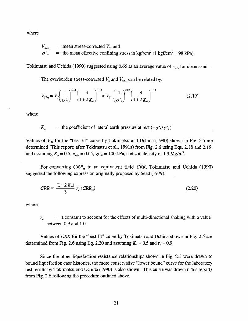
Values of VS1 for the "best fit" curve by Tokimatsu and Uchida (1990) shown in Fig. 2.5 aredetermined (This report; after Tokimatsu et al., 1991a) from Fig. 2.6 using Eqs. 2.18 and 2.19,and assuming Ko = 0.5, emin = 0.65, (J"'m = 100 kPa, and soil density of 1.9 Mg/m3
•
For converting CRRtx to an equivalent field CRR, Tokimatsu and Uchida (1990)suggested the following expression originally proposed by Seed (1979):
where
CRR = (l+2Ko) r (CRR )3 c IX
(2.20)
rc = a constant to account for the effects of multi-directional shaking with a valuebetween 0.9 and 1.0.
Values of CRR for the "best fit" curve by Tokimatsu and Uchida shown in Fig. 2.5 are
determined from Fig. 2.6 using Eq. 2.20 and assuming Ko =0.5 and r c =0.9.
Since the other liquefaction resistance relationships shown in Fig. 2.5 were drawn tobound liquefaction case histories, the more conservative "lower bound" curve for the laboratorytest results by Tokimatsu and Uchida (1990) is also shown. This curve was drawn (This report)from Fig. 2.6 following the procedure outlined above.
21

2.5.2 Relationship by Robertson et aI. (1992)
The bounding curve by Robertson et aI. (1992) was developed using field perfonnancedata from primarily sites in the Imperial Valley, California, along with data from four other
sites, as shown in Fig. 2.7. The soil at these sites contained as much as 35 % fines. Robertson
et al. corrected Vs using Eq. 2.7. The shape of their relationship was based on the analytical
results of Bierschwale and Stokoe (1984). They reasoned that the curve should pass close to
the Imperial Valley (Wildlife site) data point, since liquefaction did and did not occur at this
site during the 1987 Superstition Hills (Mw =6.5) and Elmore Ranch (Mw =6.2) earthquakes,
respectively. Robertson et al. used the magnitude scaling factors suggested by Seed (1979),similar to factors listed in Column 2 of Table 2.1, to position their curve for magnitude 7.5
earthquakes.
2.5.3 Relationship by Kayen et al. (1992)
Kayen et al. (1992) studied four sites that did and did not liquefy during the 1989 Lorna
Prieta, California, earthquake (Mw =7.0). The four sites are: Port of Richmond, Bay Bridge
Toll Plaza, Port of Oakland, and Alameda Bay Farm Island South Loop Road. The finescontent for soils at these sites ranged from less than 5 % to as much as 57 %. Values of Vs were
measured by the SCPT method and corrected for overburden stress using Eq. 2.7. Figure 2.8presents their data and bounding curve. The curve was adjusted for magnitude 7.5 earthquakesassuming a MSF of 1.19 (see Column 3 of Table 2.1), as shown in Fig. 2.5.
2.5.4 Relationship by Lodge (1994)
Lodge (1994) considered the same sites that Kayen et al. (1992) studied, as well as other
sites shaken by the 1989 Lorna Prieta earthquake. The curve by Lodge was developed as
follows. First, cyclic stress ratios for the entire soil profile at each site were calculated.
Second, available SPT blow counts were corrected for overburden pressure and energy. Soillayers with high and low liquefaction potential were identified with the procedure of Seed et al.
(1985). Soil layers with corrected blow count within 3 of the SPT-based curve were eliminated
due to uncertainties in the correlation. Third, Vs measurements from SCPT and crosshole testswere corrected for overburden stress using Eq. 2.7. Fourth, on a "meter by meter" basis, values
of VS1 and cyclic stress ratio were plotted for both layer types, those which were predicted
liquefiable and those which were predicted non-liquefiable. Fifth, published data for sitesshaken by the 1983 Borah Peak, Idaho, and 1964 Niigata, Japan, earthquakes were added to the
plot. Finally, a curve was drawn to include all liquefiable layers, as shown in Fig. 2.9. Figure
2.5 shows the curve by Lodge adjusted for magnitude 7.5 earthquakes assuming a MSF of 1.19(see Column 3 of Table 2.1).
22

ex: 0.6ex:()
Liquefaction
San Salvador, 1986M= 6.2, FC= 30 %
!M=7.5
100 200 300
Overburden Stress-Corrected Shear WaveVelocity, VS1, mls
Robertson et al.(1992)
NoLiquefaction
Borah Peak, 1983M= 7.3, Sandy Gravel.
FC = fines content
~
~ 0.4 1-------+-----....:-----1---J------1
a:sa:Q)()ca:s.....enenQ)a: Chibaken Toho Oki, 1987
eno 0.21----lm-p-e-ria-'-v-al-le-ly-,1-9-87-1---4~--1""""-/-M=16.7' FC=35 %
M= 6.6, FC= 35 %en Niigata, 1964~ M= 7.5, FC::;.10 %.....
C/)()
()>.U 0.0 L...-_----L__--J...__......L...__....L...-__.J...-_---J
o
Fig. 2.7 - Liquefaction Resistance Relationship for Magnitude 7.5 Earthquakes andCase History Data from Robertson et aI. (1992).
23.

I I 1
SiteField Performance • Port of Richmond
r- +Liquefaction ... Bay Bridge -oNo liquefaction +0 Port of Oakland
• Bay Farm Island
Kayen et al.
Liquefaction(1992)
~ -............ ...
t.+0
Range--'V
'" Nor- Liquefaction -
I I I
0: 0.60:()~
o0:~~ 0.4ctSa:(J)()s:::::ctS+-'enen(J)
a:~ 0.2oenen~+-'C/)()
()>.o 0.0
o 100 200
Overburden Stress-Corrected Shear WaveVelocity, VS1, mls
300
Fig. 2.8 - Liquefaction Resistance Relationship for Magnitude 7 Earthquake and CaseHistory Data from Kayen et al. (1992).
24

<><>
Performance• Liquefactiono No liquefaction
NoLiquefaction
Liquefaction
100 200 300
Overburden Stress-Corrected Shear WaveVelocity, VS1, m/s
1Liquefaction / noliquefaction basedon SPT criteria ofSeed et al. (1985)
2Liquefaction •based on surface t-------=4IIIU----iIT-.....::----~r--f
manifestations3Soil containscarbonate and isprobably of latestPleistocene age(Andrus, 1994;Andrus & Youd,1987)
Earthquake1989 Lorna Prieta, Calif.1
• 0 Port of Richmond, Port of Oakland,Bay Bridge, Bay Farm Island
• <> Treasure Island, Gilroy,Oakland Outer Harbor .3
• 1983 Borah Peak, Idah02 .3 Lodge....A_1_9_6_4_N_ii.:::..ga_ta.....;,_Jr-a.:,..pa_n_2__S--+----+-(1994)
ct 0.6ct(,)
lo....
o
~~ 0.4caII:Q)(,)cca-(/)
(/)Q)
a:lo.... 0.2o(/)(/)
~-(J)(,)
(,)>.() 0.01....------I-----I.------I..-----'---.....L...--......
o
Fig. 2.9 - Liquefaction Resistance Relationship for Magnitude 7 Earthquakes and CaseHistory Data from Lodge (1994).
25

2.5.5 Relationship by Andrus and Stokoe (1997)
The curve by Andrus and Stokoe (1997) shown in Fig. 2.5 was developed for theproceedings of the 1996 NCEER workshop. Several suggestions were offered at, and after, the
workshop concerning how site variables should be define, as well as the shape of the boundary
curve separating liquefaction and no liquefaction. Following the suggestions and using field
perfonnance data from 20 earthquakes and in situ Vs measurements from over 50 sites in soilsranging from clean fine sand to sandy gravel with cobbles to profiles including silty clay layers,Andrus and Stokoe constructed curves for uncemented, Holocene-age soils with various finescontent, FC. The values of Vs were corrected using Eq. 2.7. The curve for FC :s; 5 % byAndrus and Stokoe along with the case history data are presented in Fig. 2.10
The shape of the curve by Andrus and Stokoe (1997) is based on a modified relationshipbetween VS1 and CSR for constant average cyclic shear strain suggested by R. Dobry (seeSection 2.3). Andrus and Stokoe reasoned that the curve separating liquefiable and nonliquefiable soils would become asymptotic to some limiting upper value of Vsr Thisassumption is equivalent to the assumption commonly made in the SPT- and CPT-basedprocedures where liquefaction is considered not possible above a corrected blow count of about30 (Seed et al., 1985; Youd et al., 1997) and a corrected tip resistance of about 160 (Youd et al.,1997; Robertson and Wride, 1998). Upper limits for blow count and VS1 are explained by thetendency of dense soils to exhibit dilative behavior at large strains, causing negative pore waterpressures. While it is possible in a dense soil to generate pore water pressures close to theconfining stress if large cyclic strains or many cycles are applied to the soil, the amount ofwater expelled during reconsolidation is dramatically less for dense soils than for loose soils.As explained by Dobry (1989), in dense soils, settlement is insignificant and no sand boils orengineering failure take place because of the small amount of water expelled. This is importantbecause the definition of liquefaction used to classify the case histories here, as well as in thepenetration-based simplified procedures, is based on surface manifestations.
Thus, Andrus and Stokoe (1997) modified Eq. 2.11 to:
where
{( ) 2 ( J}eRR = a VSI +b 1 _1_ MSF100 V;I - VSI V;I
~I = the limiting upper value of VS1 for liquefaction occurrence, anda, b = curve fitting parameters.
26
(2.21)

100 200 300
Overburden Stress-Corrected Shear WaveVelocity, VS1, mls
o
Mw= 7.5
NoLiquefaction
Liquefaction
et0.6
Data Based on:~ Mw =5.9 to 8.3; adjusted by'- dividing CSR by (MvJ7.5)-3.3 ~5 Fines
et° Uncemented, I Content (%)Holocene-age soils
~ Average values ofVS1 and amax ,
Andrus &.2 0.4/--------+-------1---=----· Stokoe«S ~a: I (1997)
(J)()cctS...en
·00(J)
~ 0.2 t---------iI-------"!I... --t...,....""------1
o~ Fines Content~ .0 ~5%... .fJ. 6to 34 % fJ.D~ • 0 ~ 35 % Field Performance
• Liquefaction~ 0 No liquefaction() 0.0 L..-===:......J.::::._L_--l1L-----Jtt==::::I:==::::::::::J
o
Fig. 2.10 - Liquefaction Resistance Relationship for Magnitude 7.5 Earthquakes andUncemented Clean Soils of Holocene Age with Case History Data fromAndrus and Stokoe (1997).
27
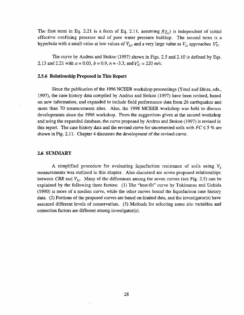
The first term in Eq. 2.21 is a form of Eq. 2.11, assuming f(Yav) is independent of initialeffective confining pressure and of pore water pressure buildup. The second term is ahyperbola with a small value at low values of VSJ ' and a very large value as VSJ approaches \Tsl.
The curve by Andrus and Stokoe (1997) shown in Figs. 2.5 and 2.10 is defined by Eqs.2.13 and 2.21 with a =0.03, b =0.9, n = -3.3, and \Tsl =220 m/s.
2.5.6 Relationship Proposed in This Report
Since the publication of the 1996 NCEER workshop proceedings (Youd and Idriss, eds.,1997), the case history data compiled by Andrus and Stokoe (1997) have been revised, basedon new information, and expanded to include field performance data from 26 earthquakes andmore than 70 measurements sites. Also, the 1998 MCEER workshop was held to discussdevelopments since the 1996 workshop. From the suggestions given at the second workshopand using the expanded database, the curve proposed by Andrus and Stokoe (1997) is revised inthis report. The case history data and the revised curve for uncemented soils with Fe ~ 5 % areshown in Fig. 2.11. Chapter 4 discusses the development of the revised curve.
2.6 SUMMARY
A simplified procedure for evaluating liquefaction resistance of soils using Vsmeasurements was outlined in this chapter. Also discussed are seven proposed relationshipsbetween eRR and VSl" Many of the differences among the seven curves (see Fig. 2.5) can beexplained by the following three factors: (1) The "best-fit" curve by Tokimatsu and Uchida(1990) is more of a median curve, while the other curves bound the liquefaction case historydata. (2) Portions of the proposed curves are based on limited data, and the investigator(s) haveassumed different levels of conservatism. (3) Methods for selecting some site variables andcorrection factors are different among investigator(s).
28

•a: 0.6a:<..:>
Data Based on:Mw = 5.9 to 8.3; adjusted by
dividing CSR by (MvJ7.5)-2.56Uncemented,
Holocene-age soilsAverage values of •
VS1and 8max
Mw=7.5
::;5 FinesI Content (%)
100 200 300Overburden Stress-Corrected Shear Wave
Velocity, VS1, mls
Fig. 2.11 - Revised Liquefaction Resistance Relationship for Magnitude 7.5 Earthquakesand Uncemented Clean Soils of Holocene Age with Case History Data fromThis Report.
29

30

CHAPTER 3
CASE mSTORY DATA AND THEIR CHARACTERISTICS
Shear wave velocity measurements have been made for field liquefaction studies atmany sites during the past fifteen years. Table 3.1 lists over 70 sites and 26 earthquakes thathave been investigated. Of the 26 earthquakes listed, 9 occurred in the United States; and theother 15 in Japan, Taiwan, and China. The field performance information for these earthquakesalong with the Vs measurements provides an important opportunity to determine therelationship between liquefaction resistance and Vs directly from case histories. A summary ofavailable case history data is presented in Appendix C. This chapter describes the site variablesand characteristics of the database.
3.1 SITE VARIABLES AND DATABASE CHARACTERISTICS
3.1.1 Earthquake Magnitude
Earthquake magnitudes for the 26 earthquakes listed in Table 3.1 range from 5.3 to 8.3,based on the moment magnitude scale. Moment magnitude is the scale most commonly usedfor engineering applications, and is the preferred scale for liquefaction resistance calculations(Youd et aI., 1997). When other magnitude scales are reported by the investigator(s), they areconverted to M w using the relationship of Heaton et al. (1982) shown in Fig. 3.1.
3.1.2 Shear Wave Velocity Measurement
Shear wave velocity measurements were made with 139 test arrays at the more than 70investigation sites listed in Table 3.1. A test array is defined in this report as the two boreholesused for crosshole measurements, the borehole and source used for downhole measurements,the cone sounding and source used for seismic cone measurements, the borehole used forsuspension logging measurements, or the line of receivers used for Spectral-Analysis-ofSurface-Waves (SASW) measurements. Of the 139 test arrays, 39 are crosshole, 21 downhole,27 seismic cone, 15 suspension logger, 36 SASW, and one is unknown.
31

Table 3.1 - Earthquakes and Sites Used to Establish Liquefaction Resistance Curves
Earthquake Moment Site ReferenceMagnitude
(1) (2) (3) (4)
1906 San Francisco, Calif. 7.7 Coyote Creek; Salinas River Youd & Hoose (1978);(North, South) Barrow (1983); Bennett &
Tinsley (1995)
1957 Daly City, California 5.3 Marina District (2, 3, 4, 5, Kayen et al. (1990);School) Tokimatsu et al. (1991b);
T. L. Youd (personalcommunication to R. D.Andrus, 1999)
1964 Niigata, Japan 7.5 Niigata City (AI, C1, C2, Yoshimi et al. (1984;Railway Station) 1989); Tokimatsu et al.
(1991a)
1975 Haicheng, China 7.3 Chemical Fiber; Construction Arulanandan et al. (1986)Building; Fishery &Shipbuilding; Glass Fiber;Middle School; Paper Mill
1979 Imperial Valley, Calif. 6.5 Heber Road (Channel fill, Bennett et al. (1981;1981 Westmorland, Calif. 5.9 Point bar); Kornbloom; 1984); Sykora & Stokoe1987 Elmore Ranch, Calif. 5.9 McKim; Radio Tower; Vail (1982); Youd & Bennett1987 Superstition Hills, Calif. 6.5 Canal; Wildlife (1983); Bierschwale &
Stokoe (1984); Stokoe &Nazarian (1984); Dobryet al. (1992); Youd &Holzer (1994)
1980 Mid-Chiba, Japan 5.9 Owi Island No.1 Ishihara et al. (1981; 1987)1985 Chiba-Tharagi-Kenkyo, Japan 6.0
1983 Borah Peak, Idaho 6.9 Andersen Bar; Goddard Youd et al. (1985); StokoeRanch; Mackay Dam et al. (1988a); Andrus et al.Downstream Toe; North (1992); Andrus (1994)Gravel Bar; Pence Ranch
1986 Event LSST2, Taiwan 5.3 Lotung LSST Facility Shen et al. (1991);Event LSST3, Taiwan 5.5 EPRI (1992)Event LSST4, Taiwan 6.6Event LSST6, Taiwan 5.4Event LSSTI, Taiwan 6.6Event LSST8, Taiwan 6.2Event LSST12, Taiwan 6.2Event LSST13, Taiwan 6.2Event LSST16, Taiwan 7.6
1987 Chiba-Toho-Oki, Japan 6.5 Sunamachi Ishihara et al. (1989)
32
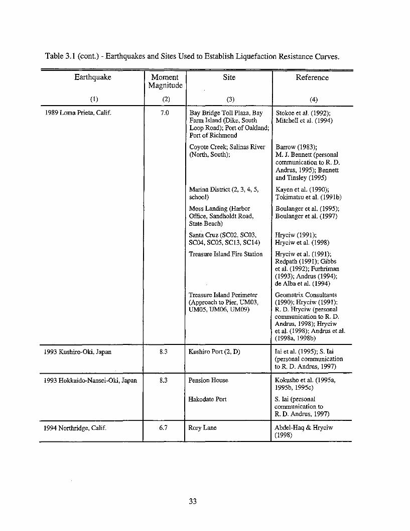
Table 3.1 (cont.) - Earthquakes and Sites Used to Establish Liquefaction Resistance Curves.
Earthquake Moment Site ReferenceMagnitude
(1) (2) (3) (4)
1989 Lorna Prieta, Calif. 7.0 Bay Bridge Toll Plaza, Bay Stokoe et al. (1992);Farm Island (Dike, South Mitchell et al. (1994)Loop Road); Port of Oakland;Port of Richmond
Coyote Creek; Salinas River Barrow (1983);(North, South); M. 1. Bennett (personal
communication to R. D.Andrus, 1995); Bennettand Tinsley (1995)
Marina District (2, 3, 4, 5, Kayen et al. (1990);school) Tokimatsu et al. (1991b)
Moss Landing (Harbor Boulanger et al. (1995);Office, Sandholdt Road, Boulanger et al. (1997)State Beach)
Santa Cruz (SC02, SC03, Hryciw (1991);SC04, SC05, scn, SCI4) Hryciw et al. (1998)
Treasure Island Fire Station Hryciw et al. (1991);Redpath (1991); Gibbset al. (1992); Furhriman(1993); Andrus (1994);de Alba et al. (1994)
Treasure Island Perimeter Geomatrix Consultants(Approach to Pier, UM03, (1990); Hryciw (1991);~05, ~06, ~09) R. D. Hryciw (personal
communication to R. D.Andrus, 1998); Hryciwet aI. (1998); Andrus et al.(1998a, 1998b)
1993 Kushiro-Oki, Japan 8.3 Kushiro Port (2, D) lai et al. (1995); S. lai(personal communicationto R. D. Andrus, 1997)
1993 Hokkaido-Nansei-Oki, Japan 8.3 Pension House Kokusho et al. (1995a,1995b, 1995c)
Hakodate Port S. lai (personalcommunication toR. D. Andrus, 1997)
1994 Northridge, Calif. 6.7 Rory Lane Abdel-Haq & Hryciw(1998)
33

Table 3.1 (cont.) - Earthquakes and Sites Used to Establish Liquefaction Resistance Curves.
Earthquake Moment Site ReferenceMagnitude
(1) (2) (3) (4)
1995 Hyogo-Ken Nanbu, Japan 6.9 Hanshin Expressway 5 Hamada et al. (1995);(3, 10, 14, 25, 29); Kobe- Hanshin ExpresswayNishinomiya Expressway Public Corporation (1998)(3, 17,23,28)
KNK; Port Island (Downhole Sato et al. (1996);Array); SGK Shibata et al. (1996)
Port Island (Common Ishihara et al. (1997);Factory) Ishihara et al. (1998)
Kobe Port (7C); Port Island Inatomi et al. (1997);(IC,2C) Hamada et al. (1995)
Kobe Port (LPG Tank Yard) S. Yasuda (personalcommunication toR. D. Andrus, 1997)
34

104 6 8Moment Magnitude, Mw
1/MJMA C? MS-\
I-- -
~~.----j:;.- -----rna
-----~ - ML_
~~.","
/. /'
~/~L-- - ------ - --~ rnb
~V
/ t;7f./ 7
'I Magnitude Scale
i/ I ML Local or Richter
y I Ms Surface wave
IMs rnb Short-period body wave
/rna Long-period body waveMJMA Japanese Meteorological
Agency
4
8
22
10
Fig. 3.1 - Relationship Between Moment Magnitude and Various Magnitude Scales(after Heaton et aI., 1982).
35
Values of Vs reported by the investigator(s) are used directly. The one exception is forthe downhole array located at the Marina District School site in San Francisco, California. Areevaluation of the field data indicates that Vs values reported for the critical layer at this siteare too high. They are recalculated using the pseudo-interval method, as discussed in Section3.2.2.
Only the crosshole measurements made with shear waves having particle motion in thevertical direction are used. Crosshole measurements near the critical layer boundary that seemhigh, and could represent refracted waves, are not included in the average.
Some Vs-values are from measurements made before the earthquake, others followingthe earthquake. No adjustments are made to compensate for changes in soil density and Vs dueto ground shaking.
3.1.3 Measurement Depth
In situ Vs measurements may be reported at discrete depths or for continuous intervals,depending on the test method. When velocities are reported for continuous intervals, as is thecase for downhole and SASW measurements, the depth to the center of each interval isassumed. Thus, if the reported Vs profile has ten velocity layers, it is assumed that the profileconsists of ten "measurements" with depths at the center of each layer.
. 3.1.4 Case History
In this report, a case history is defined as a seismic event and a test array. For example,at the Treasure Island Fire Station site, crosshole measurements were made between fivedifferent pairs of boreholes, downhole measurements were made by two different investigators,seismic cone measurements were made at one location, and SASW measurements were madealong one alignment. Thus, a total of nine case histories are identified for the Fire Station siteand the 1989 Lorna Prieta, California earthquake. At the Marina District School site, downholemeasurements were made at one location. Estimates of ground surface acceleration at this siteare available for the 1957 Daly City and 1989 Lorna Prieta earthquakes. Thus, two casehistories are identified for the Marina District School site. Combining the 26 seismic eventsand the 139 test arrays, a total of 225 case histories are obtained with 149 from the UnitedStates, 36 from Taiwan, 34 from Japan, and 6 from China.
36

The two exceptions to this definition are the Owi Island No. 1 and Moss Landing
Sandholdt Road UC-4 sites where additional subsurface information is available. At Owi
Island, pore pressure transducers recorded pore-water pressure buildup for two separate layers.At Moss Landing, inclinometer measurements indicated lateral movement in an upper loose
layer and no lateral movement in a lower dense layer. Thus, two case histories are identifiedfor each of these two test arrays.
3.1.5 Liquefaction Occurrence
It is important to realize that the occurrence of liquefaction, in this evaluation, is based
on the appearance of surface evidence, such as sand boils, ground cracks and fissures, and
ground settlement. Case histories are classified as non-liquefaction when no liquefaction
effects were observed. At the Owi Island No.1, Lotung LSST Facility, Sunamachi, Wildlife
(1987 earthquakes), and Port Island sites, the assessment of liquefaction or non-liquefaction
occurrence is supported by pore-water pressure measurements. Figure 3.2 shows the
distribution of case histories with earthquake magnitude. Of the 225 case histories, 90 areliquefaction case histories and 135 are non-liquefaction case histories.
80 r-------,------'T----,-----,----..,.-----,
Field Performance~ Liquefactiono No liquefaction 1--_--+__~5~9~_+-----I----__I
8
5 1
45
6 6.5 7 7.5
Earthquake Moment Magnitude, Mw
5.5
en.~ 60oenJ:Q)
~() 40 I------t----+----+-
o~
Q).0E:J 20 17--1----1Z
Fig. 3.2 - Distribution of Liquefaction and Non-Liquefaction Case Histories by EarthquakeMagnitude.
37

3.1.6 Critical Layer
The critical layer is the layer of non-plastic soil below the ground water table wherevalues of VSJ ' as defined in Chapter 2, and penetration resistance are generally the least, andwhere the cyclic stress ratio relative to VSJ is the greatest. Figure 3.3 presents the cumulativerelative frequency distribution for the case histories by critical layer thickness. Critical layerthicknesses range from 1 m to as much as 13 m. About 50 % of the case histories have acritical layer thickness less than 3.5 m; 90 % of the case histories have a critical layer thicknessless than 7 m.
Figure 3.4 presents the cumulative relative frequency distribution for the case historiesby average Vs measurement depth in the critical layer. The average depths of the Vsmeasurements are between 2 m and 11 m for nearly all case histories. Over 50 % of the casehistories have average measurement depths less than 5.5 m. About 90 % of the case historieshave average measurement depths less than 8 m.
Materials comprising the critical layers range from clean fine sand to sandy gravel withcobbles to profiles including silty clay layers. Figure 3.5 summarizes the average fines content(silt and clay) for the case histories grouped according to earthquake moment magnitude. Ofthe 225 case histories, 57 are for soils with 5 % or less fines, 98 for soils with 6 % to 34 %
fines, and 70 for soils with 35 % or more fines. About 20 % of the case histories are for soilscontaining more than 10 % gravel.
About 70 % of the case histories are for natural soils deposits, with many formed byalluvial processes. The other 30 % are for hydraulic or dumped fills. Eight of the fills havebeen densified by soil improvement techniques.
At least 85 % of the case histories are of Holocen~ age « 10 000 years). While the ageof the other 15 % is unknown, they are believed to be also of Holocene age.
3.1.7 Ground Water Table
The ground water table for nearly all case histories lies between depths of 0.5 m and6 m, as shown in Fig. 3.6. Nearly 60 % of the case histories have water table depths less than2 m. About 90 % of the case histories have water table depths less than 4.5 m.
Artesian pressures are reported for the Lotung Large-Scale Seismic Test (LSST)Facility site in Taiwan. At this site, the pore-water pressure distribution is assumed to varylinearly from a pressure head of 8.1 m at a depth of 7 m to a pressure head of 1.9 m at a depthof2m.
38

.' ., . ..,.' .J
•
•.J
~I
.)'It
./
100
~0
>.() 80c0)::Jc-O)
-- 60u..0)>+=ctl
Q5 40a:0)
>+=ctl"5 20E::J()
oo 2 4 6 8 10 12
Thickness of Critical Layer, m
14 16
Fig. 3.3 - Cumulative Relative Frequency of Case History Data by Critical Layer Thickness.
•• • .'II"
~I·~
J
IIt'
V1--
,,1oo 2 4 6 8 10 12 14 16
Average Depth of Vs Measurements in Critical Layer, m
100
~0
>.() 80c0)::Jc-~
60u..0)>+=ctl
Q5 40a:0)>~
20::JE::J()
Fig. 3.4 - Cumulative Relative Frequency of Case History Data by Average Depth of VsMeasurements in Critical Layer.
39

80
enQ) 60"C0...."~:J:Q)enca 400-0~
Q).cE::J 20Z
o
Fines ContentD ~5 %
f-- 06%t024%&':I ~35%
47-44
~20 18-16
~r- 13 14
6 8 ~ ~ ~ ~ 8
~ ~ ~ ~ ~~ 1 ~20: ~ .....".::-:.:. ~ 1:':=':':'1
5.5 6 6.5 7 7.5Earthquake Moment Magnitude, Mw
8
Fig. 3.5 - Distribution of Case Histories by Earthquake Magnitude and Average FinesContent.
-- .11.-.Jrl
l ...r.JJ
~I
-..
100
~0
>() 80c:Q)::JC"~
60LLQ)>
".0:;ca(j) 40a:Q)>~
20::JE::J0
oo 1 2 3 4 5 6 7
Depth to Ground Water Table, m
8
Fig. 3.6 - Cumulative Relative Frequency of Case History Data by Depth to the Ground WaterTable.
40

3.1.8 Total and Effective Overburden Stresses
Values of total and effective overburden stresses are estimated using densities reportedby the investigator(s). When no densities are reported, typical values for soils with similargrain size, penetration and velocity characteristics are assumed. In most instances, the assumeddensities are 1.76 Mg/m3 for soils above the water table and 1.92 Mg/m3 for soils below thewater table.
3.1.9 Average Peak Ground Acceleration
Average values of peak horizontal ground surface acceleration, amax, are determined byaveraging estimates reported by the investigator(s) and estimates made as part of this study
using attenuation relationships developed from published ground surface acceleration data.Since many published attenuation relationships are based on both peak values obtained fromground motion records for the two horizontal directions (sometimes referred to as the randomlyoriented horizontal component), the geometric mean (square root of the product) of the twopeak values is used. Use" of the geometric mean is consistent with the development of the SPTbased procedure (Youd et aI., 1997). For the cases in this study, the difference between thegeometric mean and arithmetic mean values is generally small, within about 5 %.
3.1.10 Average Cyclic Stress Ratio
Cyclic stress ratios, CSR, are first calculated for each "measurement" depth within thecritical layer using Eq. 2.1, and then averaged. Values of rd are estimated using the average bySeed and Idriss (1971) shown in Fig. 2.1. These rd values are used to follow the traditionalformat of the SPT- and CPT-based procedures where the magnitude scaling factor is used toaccount for all effects of earthquake magnitude.
3.1.11 Average Overburden Stress-Corrected Shear Wave Velocity
Values of Vs within the critical layer are first corrected for overburden stress using Eq.1.4, and then averaged. The number of values included in the average range from 1 to 22 (seeAppendix C). About 80 % of the case histories have 2 to 7 values in the average. Noadjustments are made for possible variations between seismic test methods due to differentsource-receiver orientations with respect to the stress state in the soil. In the calculations, eachsite is assumed to be level ground.
41

3.2 SAMPLE CALCULATIONS
Calculations for two sites shaken by the 1989 Lorna Prieta, California earthquake (Mw =7.0) are presented below to illustrate how values of CSR and overburden stress-corrected shearwave velocity, VSj ' are determined. The two sites are Treasure Island Fire Station and MarinaDistrict School.
3.2.1 Treasure Island Fire Station
Treasure Island is a man-made island located in the San Francisco Bay along the BayBridge between the cities of San Francisco and Oakland. It was constructed in 1936-37 byhydraulic filling behind a perimeter rock dike.
Extensive field tests have been conducted at the fire station on Treasure Island. Figure3.7 presents two Vs profiles for the site. The Vs profile determined by crosshole testing is fromFuhriman (1993). The other Vs profile is based on unpublished SASW test results by TheUniversity of Texas at Austin in 1992. Also presented in Fig. 3.7 is the soil profile for the site.From the description by de Alba et al. (1994), the upper 4.5 m of soil consists of silty sand fill,possibly formed by dumping. Between depths of 4.5 m and 12.2 m, the soil consists of siltysand to clayey sand, formed by hydraulic filling. Beneath the hydraulic fill are natural clayeysoils. The ground water table lies near the ground surface at a depth of 1.4 m. The criticallayer is determined to be between depths of 4.5 m and 7 m, where the soil is non-plastic, liesbelow the water table, and exhibits the lowest values of VS1 relative to the highest values ofCSR in the layer (see Fig. 5.1).
During the 1989 Lorna Prieta earthquake, a seismograph station at the fire stationrecorded ground surface accelerations. The peak values in the two horizontal accelerometerrecords are 0.16 g and 0.11 g (Brady and Shakal, 1994). Unlike recordings at otherseismograph stations located on soft-soils in the Bay area, there is a sudden drop in therecorded acceleration at about 15 seconds and small motion afterwards (Idriss, 1990). De Albaet al. (1994) attribute this behavior to liquefaction of an underlying sand. However, no sandboils or ground cracks occurred at the site. The nearest liquefaction effect observed is a sandboil located 100 m from the site (Geometric Consultants, 1990; Bennett, 1994; Power et aI.,1998). Thus, this site is classified as a non-liquefaction site during this event by the definitiongiven in Section 3.1.4.
42

Shear Wave Velocity, Vs, m/s100 200 300
Silty sandfill
(possiblydumped)
Siltysand fill
(hydraulic)----Clayeysand
----Silty
sand fill(hydraulic)
Clayeysand
Clay
Soil profileinformationfrom de Albaet al. (1994)
Data points usedfor crossholecase historydetermination
CriticalLayer
•••
•
•Data pointused for SASWcase historydetermination
5
E.c.a.Q) • 0 Crosshole dataCl for boreholes
81 & 84 from10 Fuhriman (1993) 1-1-----1-------1
-CSASW dataplotted atcenter of layersused in modelingby The Univ. ofTexas at Austin
Fig. 3.7 - Shear Wave Velocity and Soil Profiles for the Treasure Island Fire Station Site.
43
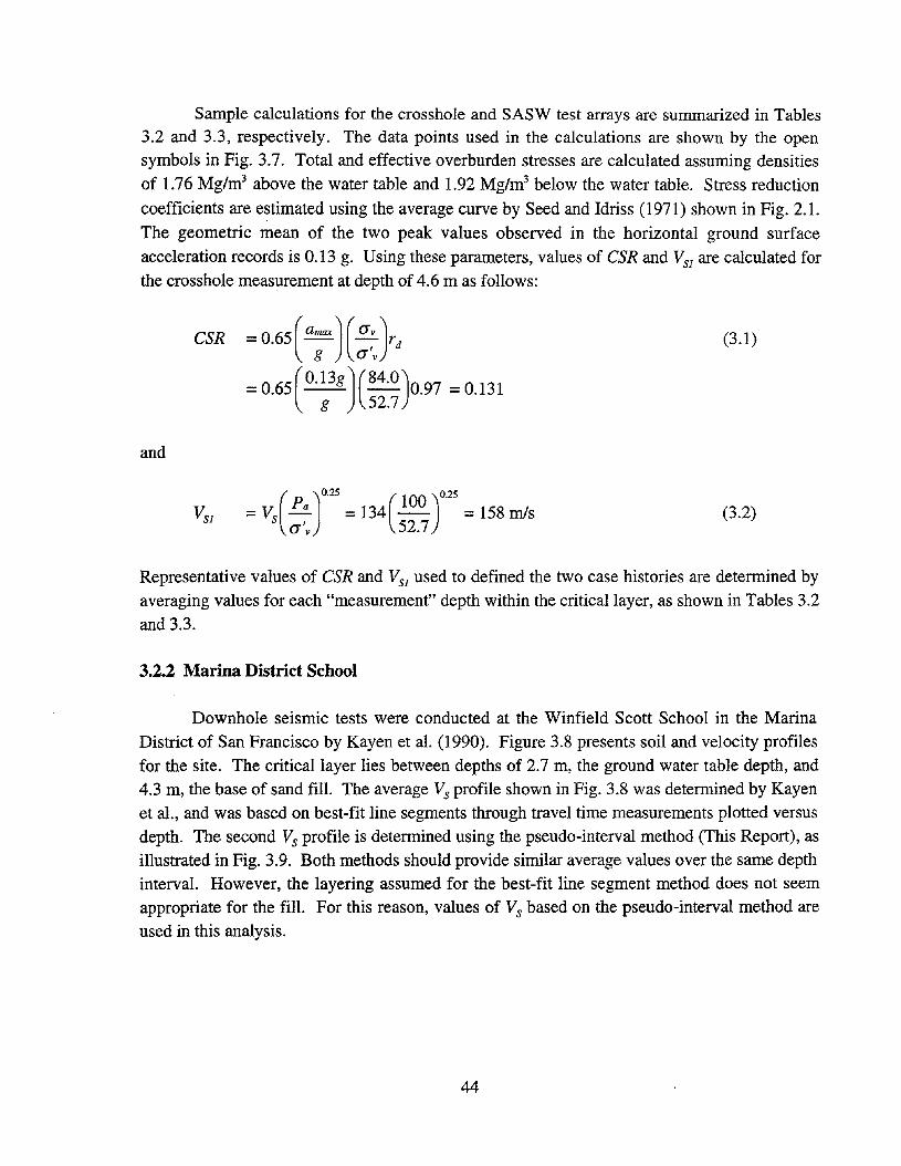
Sample calculations for the crosshole and SASW test arrays are summarized in Tables3.2 and 3.3, respectively. The data points used in the calculations are shown by the opensymbols in Fig. 3.7. Total and effective overburden stresses are calculated assuming densitiesof 1.76 Mg/m3 above the water table and 1.92 Mg/m3 below the water table. Stress reductioncoefficients are estimated using the average curve by Seed and Idriss (1971) shown in Fig. 2.1.The geometric mean of the two peak values observed in the horizontal ground surfaceacceleration records is 0.13 g. Using these parameters, values of CSR and VS1 are calculated forthe crosshole measurement at depth of 4.6 m as follows:
and
CSR =O.6S( a;X](;}
=0.65 (O.13g] (84'°)0.97 =0.131
g 52.7
( JO.25 ( )025=Vs p~ = 134 100 . = 158m1s
(J" v 52.7
(3.1)
(3.2)
Representative values of CSR and VS1 used to defined the two case histories are determined byaveraging values for each "measurement" depth within the critical layer, as shown in Tables 3.2and 3.3.
3.2.2 Marina District School
Downhole seismic tests were conducted at the Winfield Scott School in the MarinaDistrict of San Francisco by Kayen et al. (1990). Figure 3.8 presents soil and velocity profilesfor the site. The critical layer lies between depths of 2.7 m, the ground water table depth, and4.3 m, the base of sand fill. The average Vs profile shown in Fig. 3.8 was determined by Kayenet al., and was based on best-fit line segments through travel time measurements plotted versusdepth. The second Vs profile is determined using the pseudo-interval method (This Report), asillustrated in Fig. 3.9. Both methods should provide similar average values over the same depthinterval. However, the layering assumed for the best-fit line segment method does not seemappropriate for the fill. For this reason, values of Vs based on the pseudo-interval method areused in this analysis.
44

Table 3.2 - Sample Calculations for the Treasure Island Fire Station Site, Crosshole Test ArrayB1- B4, and the 1989 Lorna Prieta Earthquake.
Measured Overburden
Shear Stress Cyclic Stress-
Wave Total Effective Reduction Stress Corrected
Measurement Average Velocity, Overburden Overburden Coefficiene, Ratio3, Shear Wave
Number Depth, Vs' Stress!, Stress!, rd CSR Velocity, VSj '
m m1s kPa kPa m1s(1) (2) (3) (4) (5) (6) (7) (8)
1 4.57 134 84.0 52.7 0.97 0.13 158
2 5.49 133 111.3 60.9 0.96 0.14 150
3 6.40 144 118.5 69.2 0.95 0.14 158
---- --- - -- -- -- --Average 5.5 137 101.3 60.9 0.96 0.14 155
!Assuming water table at 1.4 m; and material densities are 1.76 Mglm3 above the water table
and 1.92 Mg/m3 below the water table.
2Based on average values determined by Seed and Idriss (1971).
3Assuming peak horizontal ground surface acceleration is 0.13 g.
Table 3.3 - Sample Calculations for the Treasure Island Fire Station Site, SASW Test Array,and the 1989 Lorna Prieta Earthquake.
Measured Overburden
Shear Stress Cyclic Stress-
Wave Total Effective Reduction Stress Corrected
Measurement Average Velocity, Overburden Overburden Coefficiene, Ratio3, Shear Wave
Number Depth, Vs' Stress!, Stress!, rd CSR Velocity, VSj '
m m1s kPa kPa m1s
(1) (2) (3) (4) (5) (6) (7) (8)
1 5.34 131 98.4 59.6 0.96 0.14 149
-- -- -- -- --- -- --Average 5.3 131 98.4 59.6 0.96 0.14 149
!Assuming water table at 1.4 m; and material densities are 1.76 Mglm3 above the water table
and 1.92 Mglm3 below the water table.
2Based on average values determined by Seed and Idriss (1971).
3Assuming peak horizontal ground surface acceleration is 0.13 g.
45

Shear Wave Velocity, Vs, mls100 200 300
Sandfill
(hydraulicor
dumped)
Naturalsand
(possiblydune orbeach)
Naturalsilty clay
(HoloceneBay Mud)
CriticalLayer
Data pointsused forcase historydetermination
Velocity and soildata from Kayenet al. (1990).
Average profile basedwater on line-fitting method
2 table -----Ii- (Kayen et aI., 1990)
--L I I'/I '----;'- - -
8
Profilebased on
1__ pseudo-
intervalI method
II (This
Report)10 L...L- .I.-I-.&.o.&-..I.-I-.L.:.I .I--I
4E.!:Q.(J)
Cl6
Fig. 3.8 - Shear Wave Velocity and Soil Profiles for the Marina District School Site(Kayen et aI., 1990).
46

ReceiverPosition 1
ReceiverPosition 2
d =distance from source to receivert=shear wave travel time
Fig. 3.9 - General Configuration ofthe Downhole Seismic Test Using the Pseudo-IntervalMethod to Calculate Shear Wave Velocity.
Many structures, pavements, and public works near the school sustained heavy damageduring the 1989 earthquake (Kayen et aI., 1990). This damage was due to liquefaction of the.sand fill. From maps prepared by Pease and O'Rourke (1995), the site lies on the margin of the1906 water front and artificial fill where about 40 mm of settlement occurred. Mapped sandboils and ground cracks lie just east of the site. Based on these observations, this site isclassified as a liquefaction site during this earthquake.
The Marina District and Treasure Island are located about 82 km from the 1989 surfacerupture. The geometric mean value of Qmax recorded at Treasure Island during the earthquake is0.13 g. The attenuation relationship by Idriss (1991) for 1989 strong ground motion recordsfrom soft-soil sites provides a median value of 0.16 g, assuming a distance of 82 km fromsurface rupture. Thus, a peak horizontal ground surface acceleration of 0.15 g, the average ofthese two estimates, is assumed in the analysis.
Sample calculations for the Marina District School site are summarized in Table 3.4.The locations of Vs measurements are assumed midway between receiver positions, as shown inFig. 3.8. Total and effective o·verburden stresses are estimated assuming densities of1.76 Mg/m3 above the water table and 1.92 Mg/m3 below the water table. The ground watertable is at a depth of about 2.7 m. Average values of CSR and VS1 defining the case history aredetermined by averaging values for the two "measurement" depths, as shown in Table 3.4
47

3.3 SUMMARY
The case history data described in this chapter are limited to level and gently slopingsites with the following characteristics:
(1) average critical layer depths less than 10m;(2) uncemented soils of Holocene age;(3) ground water table depths between 0.5 m and 6 m; and(4) all Vs measurements from below the water table.
Of the 225 case histories, 57 are for soils with 5 % or less fines (silt and clay), 98 for soils with6 % to 34 % fines, and 70 for soils with 35 % or more fines. About 20 % of the case historiesare for soils containing more than 10 % gravel. Nearly 50 % of the case histories are forearthquake magnitudes near 7.
Table 3.4 - Sample Calculations for the Marina District School Site and the 1989 Lorna PrietaEarthquake.
Measured Overburden
Shear Stress Cyclic Stress-
Wave Total Effective Reduction Stress Corrected
Measurement Average VelocityI, Overburden Overburden Coefficient3, Ratio4, Shear Wave
Number Depth, Vs' Stress2, Stress2
, rd CSR Velocity, VSJ>m mls kPa kPa mls
(1) (2) (3) (4) (5) (6) (7) (8)
1 3.02 87 52.6 49.9 0.98 0.10 104
2 3.94 136 70.0 58.2 0.97 0.11 156
-- ---- - -- -- -- --Average 3.5 112 61.3 54.1 0.98 0.11 130
IBased on pseudo-interval method.
2Assuming water table at 2.7 m; and material densities are 1.76 Mg/m3above the water table
and 1.92 Mg/m3 below the water table.
3Based on average values determined by Seed and Idriss (1971).
4Assuming peak horizontal ground surface acceleration is 0.15 g.
48

CHAPTER 4
LIQUEFACTION RESISTANCE FROM CASE HISTORY DATA
To establish the recommended curves for liquefaction resistance evaluation, cyclic
stress ratios and shear wave velocities for the 225 case histories described in Chapter 3 are
plotted in Figs. 4.1 through 4.6 for earthquakes with moment magnitudes ranging from 5.5
through 8, respectively. The plotted data have been separated into three categories: (1) sands
and gravels with average fines (silt and clay) content less than or equal to 5 %; (2) sand and
gravels with average fines content of 6 % to 34 %; and (3) sands and silts with average fines
content greater than or equal to 35 %. Also shown in Figs. 4.1 through 4.6 are therecommended liquefaction resistance curves based on Eq. 2.21. This chapter presents thedevelopment of these curves.
4.1 LIMITING UPPER VS1 VALUE FOR LIQUEFACTION OCCURRENCE
Figures 4.1 through 4.6 show that the available case history data above a cyclic stress
ratio of about 0.35 are limited. Thus, current estimates of V~I rely in part on penetration-shear
wave velocity correlations.
In the SPT-based procedure, a corrected blow count of 30 is assumed as the limitingupper value for liquefaction occurrence in clean sands above eRR of 0.6 and magnitude 7.5earthquakes (Seed et aI., 1985; Youd et aI., 1997). Table 4.1 presents estimates of equivalentVS1 for corrected blow count of 30. The relationship by Ohta and Goto (1978) modified to blowcount with theoretical free-fall energy of 60 % (Seed et aI., 1985) suggests equivalent VS1
values of 207 mls for Holocene sands and 227 mls for Holocene gravels, assuming that a depth
of 10m is equivalent to an overburden stress of 100 kPa. The stress-corrected crosshole
measurements collected by Sykora (l987b) for Holocene sands and non-plastic silty sands
below the ground water table with corrected blow count between 25 and 35 exhibit an averagevalue of 206 mls and a standard deviation of 41 mls. The correlation by Rollins et al. (l998a)provides a best-fit value of 232 mls for Holocene gravels with corrected blow count of 30.
49

Mw = 5.5
NoLiquefaction
Field Performanceo No liquefaction
0000 00000
0000
Liquefaction
100 200 300Overburden Stress-Corrected Shear Wave
Velocity, V81, m/s
Fines Contento <5%t:. 8 to 12 %o ~35%
Data Based on:Mw=5.3 to 5.5Average values of
VS1 and amaxUncemented,
Holocene-age soils
a: 0.6
~;:::35 20 $5 Fines
III Content (%)
III~
~ 0.41-------1------//-/-4-------1a:CDocCd+-'enenCDa: 0.2 1--------I-----H.J.~-_4_-----__I'-oenen~+-'enoo~o 0.0 L...-__L...-_---I__---I.__---L__---L.__--J
o
Fig. 4.1 - Case History Data for Earthquakes with Magnitude Near 5.5 Based onOverburden Stress-Corrected Shear Wave Velocity and Cyclic Stress Ratiowith Recommended Liquefaction Resistance Curves.
50

Mw=6
NoLiquefaction
Field PerformanceA Liquefactionl1 No liquefaction
e
e
Liquefaction
~
100 200 300
Overburden Stress-Corrected Shear WaveVelocity, VS1, mls
Fines Contentl1A 10 to 22 %oe ~35 %
0.6......---r---r----r-----r----.,..----...ce:ce:()
Data Based on:Mw= 5.9 to 6.2
~ Average values of ;::::3520:::;;5 Fines~ VS1 and amax II Content (%)U) Uncemented,() Holocene-age soils II~ 0.41--------+-----,-,-+-,------I
ex:CD()Cccs...enenCD
ex: 0.2 I---------f----:~-_+I_,I__--+---------f~
oenenCD~...en()
()>.o 0.0 ~--.l----.l----"'----"'----~-----I
o
Fig. 4.2 - Case History Data for Earthquakes with Magnitude Near 6 Based onOverburden Stress-Corrected Shear Wave Velocity and Cyclic Stress Ratiowith Recommended Liquefaction Resistance Curves.
51

NoLiquefaction
Field Performance~ Liquefaction~ No liquefaction
Mw= 6.5
;:::35 20 ~5 FinesContent (%)
Liquefaction
100 200 300Overburden Stress-Corrected Shear Wave
Velocity, VS1, m/s
Data Based on:Mw =6.5 to 6.7Average value of
VS1and amaxUncemented,
Holocene-age soils
0.0 r....-__..l.....-__""""'-__...I.-__--"-__........__.....I
o
0: 0.6
~
~
o 0.41---------;----....0----.::-:-+-------1
caa:(J)occtS-enen(J)
a:"- 0.2 t--------+.-----:~~_+_.H___t------___I0 0 0en ~en Fines Content~ ~~ 10 to 22 %-en o. ~35 %oo~()
Fig. 4.3 - Case tIistory Data for Earthquakes with Magnitude Near 6.5 Based onOverburden Stress-Corrected Shear Wave Velocity and Cyclic Stress Ratiowith Recommended Liquefaction Resistance Curves.
52

o
Mw=7
NoLiquefaction
o
oField Performance
A Liquefactionl:i. No liquefaction
~35 20 =:;5 FineslA , I Content (%)
•A 6"'
Liquefaction•
100 200 300Overburden Stress-Corrected Shear Wave
Velocity, VS1, mls
Fines Contento. <5%l:i.A 6 to 26 %oe > 35 %
Data Based on:Mw = 6.9 to 7.0Average value of
VS1and 8maxUncemented,
Holocene-age soils
0.0 L...-__.l..-__.l..-__.l..-__.l..-__..&....-_---I
o
ct: 0.6ct:()
•o •
011• l:i.• •...., ......<5 0.2 J---------f-A~.:-:'A-A--=::.....'-+-I f--t~*""'""--------I
enen~.....(j)()
()~()
-o1a 0.4a:CD()cctS.....enenCDa:
Fig. 4.4 - Case History Data For Earthquakes with Magnitude Near 7 Based onOverburden Stress-Corrected Shear Wave Velocity and Cyclic Stress Ratiowith Recommended Liquefaction Resistance Curves.
53

100 200 300
Overburden Stress-Corrected Shear WaveVelocity, VS1, m/s
a: 0.6a: Data Based on: Mw= 7.50 Mw = 7.3 to 7.7:l... Average value of0 ~35 20:::;5 Fines
a: VS1 and amax , , Content (%)
~Uncemented,
Holocene-age soils , ,~
00.4+-'
I I(tj
a:CD(,)
Liquefactionc •(tj+-'en
Noen(1) Liquefactiona::l... 0.21---------I----------Jr--I-I4--------1oenen Fines Content~ o. <5%(j) "14%(,) o. > 35 % Field PerformanceC3 • Liquefaction~ 0 No liquefaction() 0.0 L--__.L..-__.L..-__.L..-__..L-...__...I..-_----'
o
Fig. 4.5 - Case History Data for Earthquakes with Magnitude Near 7.5 Based onOverburden Stress-Corrected Shear Wave Velocity and Cyclic Stress Ratiowith Recommended Liquefaction Resistance Curves.
54
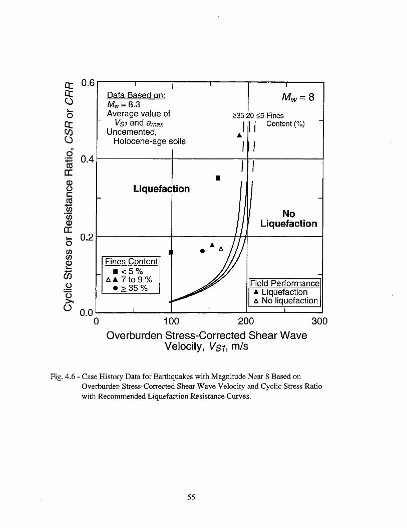
100 200 300Overburden Stress-Corrected Shear Wave
Velocity, VS1, m/s
ce: 0.6ce: Data Based on: Mw=8(,) Mw = 8.3~ Average value of0 ;:::35 20 ~5 Fines
ce: VS1 and amax
"'Content (%)
CI) Uncemented, ...(,) Holocene-age soils , ,~
00.4+-'
I IctSa:CD •(,) LiquefactioncctS+-'en NoenCD Liquefactiona:~ 0.2 t---------1-------I-+-It---------Ioen~ Fines Content~CiS _<5%(,) l!. ... 7 to 9 % Field Performance(,) • > 35 % ... Liquefaction~ l!. No liquefactiono 0.0 '--__..&...-__-'--__...&.-__...l.-__......a-__--I
o
Fig. 4.6 - Case History Data for Earthquakes with Magnitude Near 8 Based onOverburden Stress-Corrected Shear Wave Velocity and Cyclic Stress Ratiowith Recommended Liquefaction Resistance Curves.
55

Table 4.1 - Estimates of Equivalent VSJ for Holocene Sands and Gravels Below the GroundWater Table with Corrected SPT Blow Count of 30.
EquivalentReference Relationship VS] Estimate Assumptions
(mls)(1) (2) (3) (4)
Ohta& Vs =69 (N/.l73 l·195 F]F2 207 1. f; =60/67 N60
Goto ...for Holocene 2. 60 =30(1978); also ~ =SPT blow count sands 3. z =10 m is equivalenttogiven in measured in Japanese an overburden stress ofreport by practice 227 100 kPaSykora z =depth, m ...for Holocene 4. All measurements are(1987a, F] =1.00 for Holocene- gravels from below the groundpage 29) age soils water table
F2 =1.085 for sands;1.189 for gravel
...best-fit relationship for 289sets of SPT and Vsmeasurements from Japan
Sykora Correlation between (NJ)60 and 206 1. Average for VSJ values(1987b, crosshole Vs' normalized to ...for Holocene with (NJ)60 betweenpage 90); effective overburden stress, sands and non- 25 and 35This Report measurements for Holocene plastic silty 2. a'v =100 kPa
sands and non-plastic silty sands below thesands below the ground water water tabletable at sites in U.S.A.; 16 sets ...standardof measurements (with known deviation isSPT equipment) 41 mls
Rollins et Vs=53 (N60
)O.19 (a'v)OI8 232 1. N60 = 30al. (1998a) ...for Holocene 2. a'v =100 kPa
...best-fit relationship using gravels 3. All measurements areequivalent N60-values from ...most of data from below the groundBecker Penetration Tests and lie within water tableVsmeasurements; 186 points ±25 % offrom 7 Holocene gravel sites relationship
This ReportVSJ =BJ [(Nl)6ot
2 204 1. Average for VSj(see Fig. .. .for Holocene with (Nj )60 =304.7)
B j =93.2 ± 6.5clean sands 2. a'v =100 kPabelow the water 3. Corrected blow count
B2 =0.231 ± 0.022 table based on procedures
...best-fit relationship for ...residual given in Seed et al.standard (1985) and Robertsonuncemented, Holocene-age deviation is and Wride (1997; 1998)sands with less than 10 % non-
plastic fines; 25 sets of average 12 mls
SPT and Vs measurements allfrom below the water table
56

Rollins et al. noted that the majority of the data analyzed fall within ±25 % of their correlation.Figure 4.7 presents average values of VSJ and corrected blow count for soil layers with less than10 % fines at several sites listed in Table 3.1. Also shown in Fig. 4.7 is the best-fit relationshipfor the plotted data. The plotted data exhibit a mean VSJ value of 204 mls at a corrected blow
count of 30 and a residual standard deviation, Sres' of 12 mls.
In the CPT-based procedure, a normalized cone tip resistance of 160 is assumed as thelimiting upper value for liquefaction occurrence in clean sand above eRR of 0.6 and magnitude7.5 earthquakes (Youd et aI., 1997; Robertson and Wride, 1998). Figure 4.8 presents averagevalues of VSJ and normalized tip resistance for soil layers with less than 10 % fines at several
sites listed in Table 3.1. Also shown in Fig. 4.8 is the best-fit relationship for the plotted data.
Table 4.2 summarizes the general characteristics of the plotted data and best-fit relationship.
The plotted data exhibit a mean VSJ value of 193 mls at a normalized tip resistance of 160 and aresidual standard deviation of 19 mls.
From these estimates, a VSJ value of 210 mls is assumed equivalent to a corrected blowcount of 30 and normalized tip resistance of 160 in clean sands. A limiting upper VSJ value of210 mls for liquefaction occurrence is less than the general consensus value of 230 mls agreedupon at the 1998 MCEER workshop. Figures 4.7 and 4.8 have been added to this report toprovide additional evidence to support the use of 210 mls as the limiting upper value of VSJ forclean sands and gravels.
Table 4.2 - Estimates of Equivalent VSJ for Holocene Sands and Gravels Below the GroundWater Table with Normalized Cone Tip Resistance of 160.
EquivalentReference Relationship VSJ Estimate Assumptions
(mls)(1) (2) (3) (4)
This Report VSJ=BJ (QcIN)B2 193 1. Average for VSJ(see Fig. ...for Holocene with qcIN =1604.8) BJ =88.2 ± 15.5 clean sands 2. a'v =100 kPa
B2 =0.154 ± 0.037 below the water 3. Normalized tiptable resistance based on
...best-fit relationship for ...residual procedures given inuncemented, Holocene-age standard Robertson and Wridesands with less than 10 % non- deviation is (1997; 1998)plastic fines; 23 sets of average 19m1sSPT and Vs measurements allfrom below the water table
57

50
FinesContent, %
~8 53
Mean + 1Sres
\--.1-
10 20 30 40
Corrected Blow Count, (Nt)60
Location° Moss Landing[J Treasure Islandv Port of Oakland & Bay
Bridge Toll Plaza<> Salinas River, Southli. Hakodata & Kushiro Ports
s-etSCD..cCf)
"'C~CD E 250.....o ~
CD--
~~'1>:-en:!: 200 1------+----~:.....-__,~~1-_-=-~ -4--~-----<Ien 0 7 10 _-CD 0 6 --~ CD .....~ ..........Cf» 3C CD Data based on:CD > Average values of VS1'"E etS 150 1----::iO.~_f_,.L...\_~::...-___+---_1 (N1)60, & fines content:::J s: Sands with less than 10 %-e Mean, non-plastic fines~ V
S1=93.2 [(N
1)60]O.231 Measurements from belowo ground water table
Fig. 4.7 - Variations in VSj with (Nj )60 for Uncemented, Holocene-age Sands with Lessthan 10 % Non-Plastic Fines.
58

Mean;VS1 =88.2 (%1N)O.154
FinesContent, %
Data based on:Average values of VS1' %1N' & fines contentSands with less than 10 % non-plastic finesMeasurements from below ground water table
Locationo Moss Landingo Treasure Islandv Port of Oakland &Bay
Bridge Toll Plaza<> Salinas River, Southt:. Hakodata & Kushiro
Ports
50 100 150 200 250
Normalized Cone Tip Resistance, Qc1N
~
~0,).cC/)
""O~0,) E 250..-() 0,)'1'-
~~() - D.>0-~ ~ 200 ~----+------J.-~:':::'-=------+-~--=J..-~~~1:Q262
0,)0
b)~ --,---C 0,) 20 Mean - 1Sres
~ ~ 150 ~--~-=-,"~=-----=-+----+----+------1:;$.0~
0,)
>o
Fig. 4.8 - Variations in VS1 with Qc1N for Uncemented, Holocene-age Sands with Less than10 % Non-Plastic Fines.
59
For soils with fines content greater than 35 %, the SPT-based chart by Seed et al. (1985)
indicates a limiting upper corrected blow count of about 21 for liquefaction occurrence above
CRR of 0.6. Table 4.3 presents estimates of equivalent VS1 for blow count of 21. The
relationship by Ohta and Goto (1978) suggests equivalent VS1 values of 195 mls for Holocene
sands and 214 mls for Holocene gravels. The stress-corrected crosshole collected by Sykora
(l987b) for Holocene sands and non-plastic silty sands below the ground water table with
corrected blow count between 16 and 26 exhibit an average value of 199 mls and a standard
deviation of 36 mls. The correlation by Rollins et al. (l998a) provides a best-fit value of 217
mls for Holocene gravels. From these estimates, a VS1 value of 195 mls is assumed equivalent
to a corrected blow count of 21 in non-plastic soils with fines content;;::: 35 %.
To permit the liquefaction resistance curves for magnitude 7.5 earthquakes shown in
Fig. 4.5 to have VS1 values between 195 mls and 210 mls at CRR near 0.6, values of V;l are
assumed to range from 200 mls to 215 mis, respectively. The relationship between V;l and
fines content can be expressed by:
where
V;l = 215 mls
V;l = 215 - 0.5(FC-5) mls
V;l = 200 mls
for sands and gravels with FC :::; 5 % (4.1 a)
for sands and gravels with 5 % < FC < 35 % (4.lb)
for sands and silts with FC;;::: 35 % (4.lc)
FC = the average fines content in percent by mass.
The CRR-VS1 curves shown in Figs. 4.1 through 4.6 provide reasonable bounds for the
case history data shown above a cyclic stress ratio of 0.35, further supporting the use of V;lvalues given in Eq. 4.1.
60

Table 4.3 - Estimates of Equivalent VSj for Holocene Sands and Gravels Below the Ground
Water Table with Corrected SPT Blow Count of 21.
EquivalentReference Relationship VSj Estimate Assumptions
(rn/s)(1) (2) (3) (4)
Ohta& Vs =69 (Nl.173 Z°.195 FjF2 195 1. fj =60/67 N60Goto ...for Holocene 2. 60 =21(1978); also ~ =SPT blow count sands 3. Z =10 m is equivalent togiven in measured in Japanese an overburden stress ofreport by practice 214 100 kPaSykora Z =depth, m ..Jor Holocene 4. All measurements are(1987a, F j =1.00 for Holocene- gravels from below the groundpage 29) age soils water table
F2 =1.085 for sands;1.189 for gravel
...best-fit relationship for 289sets of SPT and Vsmeasurements from Japan
Sykora Correlation between (Nj )60 and 199 1. Average for VSj values(1987b, crosshole Vs' normalized to ...for Holocene with (Nj )60 betweenpage 90); effective overburden stress, sands and non- 16 and 26This Report measurements for Holocene plastic silty 2. a'v =100 kPa
sands and non-plastic silty sands below thesands below the water table at water tablesites in U.S.A.; 31 sets of ...standardmeasurements (with known deviation isSPT equipment) 36 rn/s
Rollins et Vs =53 (N60
)O.19 (a'v)018 217 1. N60 =21al. (1998a) ...for Holocene 2. a'v =100 kPa
...best-fit relationship using gravels 3. All measurements are
equivalent N60-values from ...most of data from below the ground
Becker Penetration Tests and lie within. water tableVs measurements; 186 points ±25 % offrom 7 Holocene gravel sites relationship
61,

4.2 CURVE FITTING PARAMETERS, a AND b
The curve fitting parameters a and b in Eq. 2.21 can be approximated from the casehistory data assuming the values of V~l given in Eq. 4.1 and a MSF relationship. By assuming
a MSF relationship, one can adjust the cyclic stress ratios for the case history data to magnitude7.5 as follows:
where
CSR = CSR7.5 MSF
CSR = the cyclic stress ratio, andCSR7.5 = the CSR corrected to magnitude 7.5.
(4.2)
Three MSF relationships representing the range of proposed magnitude scaling factors areconsidered below to establish the values of a and b.
4.2.1 Magnitude Scaling Factors Recommended by 1996 NCEER Workshop
4.2.1.1 Lower Bound of Recommended Range-Figure 4.9 presents the case historydata for magnitude 5.9 to 8.3 earthquakes adjusted using the lower bound for the range ofmagnitude scaling factors recommended by the 1996 NCEER workshop (Youd et aI., 1997).The lower bound is defined by Eq. 2.13 with n = -2.56, as discussed in Section 2.4.1. Alsoshown in Fig. 4.9 are three liquefaction resistance curves for earthquakes with magnitude near7.5 and various fines content. The three curves were determined through an iterative process ofvarying the values of a and b until nearly all the liquefaction case histories were bound by thecurves with the least amount of non-liquefaction case histories in the liquefaction region. Ofthe 90 liquefaction case histories, only two case histories incorrectly lie in the no liquefactionregion. The final values of a and b used to draw the curves in Fig. 4.9 are 0.022 and 2.8,respectively.
62

•
Mw =7.5Data Based on:Mw = 5.9 to 8.3; adjusted by
dividing CSR by (MJ7.5)-2.56Uncemented,
Holocene-age soilsAverage values of ...
VS1 and 8max
0: 0.6
~
100 200 300Overburden Stress-Corrected Shear Wave
Velocity, VS1, mls
Liquefaction
~
o 0.4 t--------+---...---~,....r-;-------1~ ti. ..'"u ... ...a:CD()C
~ Noenen LiquefactionCD 0~ 0.2 1-------.-.JIII---=-...-O-'~1i1------___1o~ Fines Content~ .0 <5%en ... ti. 6 to 34 %() • 0 ~ 35 % Field Performance
• Liquefaction~ 0 No liquefactiono 0.0 L_--L__.L_--L!L_~===:::J:====:::J
o
Fig. 4.9 - Curves Recommended for Calculation of eRR from Shear Wave VelocityMeasurements Along with Case History Data Based on Lower BoundValues of MSF for the Range Recommended by the 1996 NCEERWorkshop (Youd et al., 1997) and Td Developed by Seed and Idriss (1971).
63

The two liquefaction case histories in Fig. 4.9 that lie in the no liquefaction region arefor the Treasure Island UM05 and UM09 sites. The UM05 and UM09 sites are located alongthe perimeter of Treasure Island. Mapped liquefaction effects generated by the 1989 LornaPrieta earthquake near the UM05 site are ground cracks with 50 to 90 mm of horizontal
displacement (R. D. Hryciw, personal communication to R. D. Andrus, 1998; Power et aI.,
1998). The nearest mapped sand boil is located 60 m away from the site. At the UM09 site, as
much as 90 mm of vertical displacement was observed adjacent to a building located 60 m
inland from the site. These displacements are small compared to the meters of displacementthat are expected to occur during larger ground shaking. Thus, liquefaction was marginal at theUM05 and UM09 sites, and sloping ground may have been a factor. It should be noted thatsimilar evaluations are obtained using the SPT and CPT data for these sites. The SPT- andCPT-based evaluations for the UM05 site are discussed in Section 4.3.1.
4.2.1.2 Upper Bound of Recommended Range-Figure 4.10 presents the case historydata for magnitude 5.9 to 8.3 earthquakes adjusted using the upper bound for the range ofmagnitude scaling factors recommended by the 1996 NCEER workshop (Youd et aI., 1997).The upper bound is defined by Eq. 2.13 with n = -3.3, as discussed in Section 2.4.1. Alsoshown in Fig. 4.10 are the same three curves from Fig. 4.9. Many case history data plot lowerin Fig. 4.10 than in Fig. 4.9, since the earthquake magnitude is less than 7.5 for most of thedata. The downward shift in the liquefaction data points near the curves at CRR of about 0.08is less than 0.01. This difference is not significant, and is within the accuracy of the plottedcase history data.
4.2.2 Revised Magnitude Scaling Factors Proposed by Idriss (1999)
Figure 4.11 presents the case history data for magnitude 5.9 to 8.3 earthquakes adjustedusing the revised magnitude scaling factors and stress reduction coefficients proposed by Idriss(1999 as discussed in Section 2.4.2. Also shown in Fig. 4.11 are the same three liquefactionresistance curves from Fig. 4.9. Many of the case history data shown in Fig. 4.11 plot higherthan case history data in Fig. 4.9, since the earthquake magnitude is less than 7.5 for most ofthe data. The upward shift in the liquefaction data points near the curves at CRR of about 0.08is less than 0.01. This difference is also not significant, and is within the accuracy of theplotted case history data.
64

o
Mw =7.5
/)" NoLiquefaction
2::35 20 ~5 FinesContent (%)
Liquefaction
Data Based on:Mw = 5.9 to 8.3; adjusted by
dividing CSR by (Mv/7.5)-3.3Uncemented, _
Holocene-age soilsAverage values of
V81 and amax It.
ex: 0.6
~~
oex:~o 0.4t--------+------~~----___I+-'ctj
a::Q)occtj+-'enenQ)
~ 0.2 t-----------ir--- .....__....,...,H-t----L...L...-------f
o~ Fines Content~ .0 <5%en It. /)" 6 to 34 %o • 0 ~ 35 % eld Performance
O /),,It:1e e QnQ • Liquefaction>. ~ ~vov 0 No liquefactiono 0.0 L-_--L__l-_---l..!L_~~==r=::==::::J
o 100 200 300
Overburden Stress-Corrected Shear WaveVelocity, VS1, mls
Fig. 4.10 - Curves Recommended for Calculation of eRR from Shear Wave VelocityMeasurements Along with Case History Data Based on Upper Bound Valuesof MSF for the Range Recommended by the 1996 NCEER Workshop (Youdet al., 1997) and rd Developed by Seed and Idriss (1971).
65
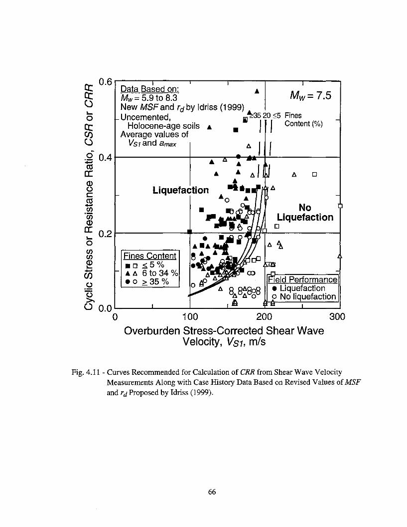
o
leld Performance• Liquefactiono No liquefaction
100 200 300
Overburden Stress-Corrected Shear WaveVelocity, VS1, mls
Fines Content.0 <5%... A 6 to 34 %• 0 ~35 %
ct 0.6
~Data Based on: ... M 7 5Mw = 5.9 to 8.3 w= .New MSF and rd by Idriss (1999)
<5 Uncemented iJ~35 20 ~5 Finesct Holocene-age soils... • , I Content (%)~ Average values of\"..J~ VS1 and 8max A I I.0 0.4 I--------+---...-....- ...:.....+-~----___l
~ - ...~ ... ...~ .a .- Liquefaction·~ "'0 ...00 No~ Liquefaction~ 0.2 f-- --III-- .......~~D-----__1
oenen~+-'C/)(.)
(.)>.() 0.01....---...1....---...1.---...1.---.....1.---...........-----1
o
Fig. 4.11 - Curves Recommended for Calculation of eRR from Shear Wave VelocityMeasurements Along with Case History Data Based on Revised Values of MSFand rd Proposed by Idriss (1999).
66

The differences between the MSF and rd relationships proposed by Idriss (1999) and therelationships recommended by the 1996 NCEER workshop (Youd et aI., 1997) are significantat magnitudes less than about 7 (see Fig. 2.4). Figure 4.12 presents two liquefaction resistancecurves for earthquakes with magnitude near 5.5 and clean soils (FC S; 5 %). The upper curvewas obtained by multiplying values of CRR defining the curve for FC S; 5% in Fig. 4.9 by 2.2,the lower MSF recommended by the 1996 NCEER workshop for magnitude 5.5 earthquakes(see Eq. 2.13 with n =-2.56). The lower curve was obtained by multiplying values of CRRdefining the curve for FC S; 5 % in Fig. 4.9 by 1.68, the MSF proposed by Idriss (1999) formagnitude 5.5 earthquakes (see Eq. 2.15). Also shown in Fig. 4.12 are the available casehistory data for clean sands determined using average stress reduction coefficients proposed by
Seed and Idriss (1971) and Idriss (1998). The two curves in Fig. 4.12 exhibit differences in
CRR of about 0.02 at VS1 =100 mls and 0.1 at VS1 =200 mls.
4.3 RECOMMENDED CRR-VS1 CURVES
From the discussion presented in Sections 4.1 and 4.2, the recommended CRR-VS1
curves are defined by Eqs. 2.13, 2.21, and 4.1 with a = 0.022, b = 2.8, and n = -2.56. The valueof -2.56 for n is recommended for determining magnitude scaling factors because it providesmore conservative CRR-VS1 curves than -3.3 for magnitude less than 7.5. While the magnitudescaling factors defined by Eq. 2.13 with n =-2.56 provide less conservative CRR-VS1 curvesthan the factors proposed by Idriss (1999) for magnitudes less than 7.5, the findings ofAmbrasey (1988), I. M. Idriss (personal communication to T. L. Youd, 1995), Arango (1996),Youd and Noble (1997), and the case history data presented in this report (see Figs. 4.2 and 4.3)support their use.
The recommended CRR-VS1 curves are shown in Figs. 4.1 through 4.6 for differentmagnitude earthquakes. The curves are dashed above CRR of about 0.35 to indicate that theyare based on limited field performance data. The curves do not extend much below 100 mis,since there are no field data to support extending them to the origin.
67
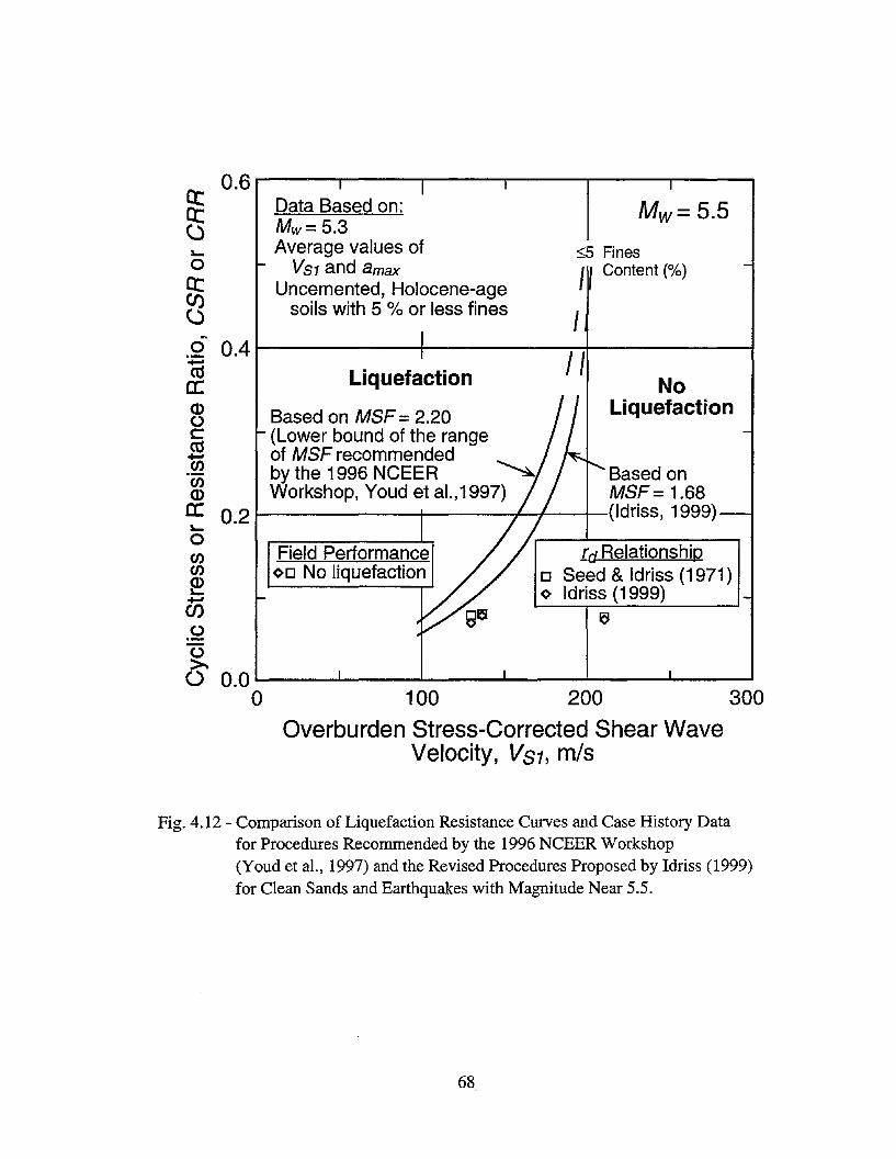
Mw=5.5
NoLiquefaction
:::;5 FinesJ Content (%)
J
I J
[d Relationshipo Seed & Idriss (1971)o Idriss (1999)
100 200 300
Overburden Stress-Corrected Shear WaveVelocity, VS1, mls
Field Performance00 No liquefaction
Based onMSF= 1.68
I---------+----~I--___l_-(Idriss, 1999)
ct0.6
Data Based on:ct Mw= 5.3()~ Average values of0 VS1 and 8maxct Uncemented, Holocene-ageCI) soils with 5 % or less fines()
0 0.4......ca Liquefactiona:Q)
Based on MSF = 2.20(,)c (Lower bound of the rangeca of MSF recommended......en by the 1996 NCEERenQ) Workshop, Youd et al.,1997)a: 0.2~
oenen~......en(,)
(,)>.() 0.0 L...-__...a..-__-L-__....L....__--L-__--'-__--I
o
Fig. 4.12 - Comparison of Liquefaction Resistance Curves and Case History Datafor Procedures Recommended by the 1996 NCEER Workshop(Youd et aI., 1997) and the Revised Procedures Proposed by Idriss (1999)for Clean Sands and Earthquakes with Magnitude Near 5.5.
68,

4.3.1 Correlations Between Vsz and Penetration Resistance
By plotting values with equal CRR, on can obtain Correlations between VS1 and
corrected penetration resistance from the recommended CRR-VS1 relationships given in Fig. 4.5
and the 1996 NCEER workshop recommended SPT- and CPT-based relationships for
magnitude 7.5 earthquakes (Youd et aI., 1997).
4.3.1.1 Corrected SPT Blow Count-Figure 4.13 presents the correlation of VS1 with
(NZ)60 for clean soils (~ 5 % fines) based on the recommended CRR-VS1 and CRR-(N1)60relationships. Also shown are the field data and mean curve for sands with less than 10 % non
plastic fines from Fig. 4.7. The correlation derived from the CRR relationships lies between the
mean and the mean +ISm curves. The flatter slope below (N)60 of 6 exhibited by the CRRbased correlation can be explained by different assumed minimal values of CRR. The CRR-VS1relationship for magnitude 7.5 earthquakes and FC ~ 5 % shown in Fig. 4.5 provides a CRR of
0.033 for Vsz =100 mis, the lowest VS1 value shown in the figure. The 1996 NCEER workshop
recommended a CRR value of 0.05 for (N1)60 =O. The difference between minimal values of
CRR is small, and is near the accuracy of both procedures.
The CRR-based curve shown in Fig. 4.13, along with the plotted field data, provide a
simple method of comparing the VS1- and (N)6o-based liquefaction evaluation procedures. Bothprocedures will provide similar predictions of liquefaction potential, when the data point lies on
the CRR-based curve. When the data point plots below the CRR-based curve, the Vs1-basedliquefaction evaluation procedure provides the more conservative prediction; and when the data
point plots above the CRR-based curve, the SPT-based liquefaction evaluation procedure
provides the more conservative prediction. Since most of the data points shown in Fig. 4.13
plot below the CRR-based curve, the Vs1-based procedure provides an overall more
conservative prediction of liquefaction resistance than does the SPT-based procedure for these
sites.
The data point for the Treasure Island UM05 site, which incorrectly lies in the region ofno liquefaction shown in Fig. 4.9, plots just below the CRR-based curve, as shown in Fig. 4.13.Thus, this case history also incorrectly plots in the region of no liquefaction on the SPT-basedliquefaction evaluation chart. Furthermore, the SPT-based procedure provides a slightly lessconservative prediction of liquefaction resistance than the shear-wave-based procedure for this
case history.
Although the CRR-based curve shown in Fig. 4.13 generally trends parallel to the mean
curve, there is a small hump between ,corrected blow counts of 8 and 26. This hump suggests
that either the CRR-Vsz relationship is more conservative or the CRR-(Nz)6o relationship is less
conservative in this range.
69

50
FinesContent, %
~8 53
Mean + 1Sres
\--1-
10 20 30 40
Corrected Blow Count, (N1)60
Mean,VS1 =93.2 [(N1)60]O.231
Curve implied by the recommendedCRR- VS1 relationship and the 1996NCEER Workshop recommendedCRR-(N1)60 relationship(Youd et al. , 1997)
:....as0).cen-c~0) E 250.....o O)'t-
~~Y:>.en :t::: 200 I------+------:\-::~....."""""::~~ _-----=---=-.>.L -+----'-'\-----1enO0)0:....-..... 0)en>C 0) Location
~ ~ 150 1----=ill~---t-.~--=--+_--_1 0 Moss Landing~ :> 0 Treasure Island_ > v Port of Oakland & Bay-e Bridge Toll Plaza0) <> Salinas River, South6 ~ Hakodata & Kushiro Ports
Fig. 4.13 - Relationships Between (Nj )60 and VSj for Clean Sands Implied by the RecommendedCRR-VS1 Relationship and the 1996 NCEER Workshop Recommended CRR-(Nj )60
Relationship (Youd et aI., 1997) with Field Data for Sands with Less than 10 %
Fines.
70
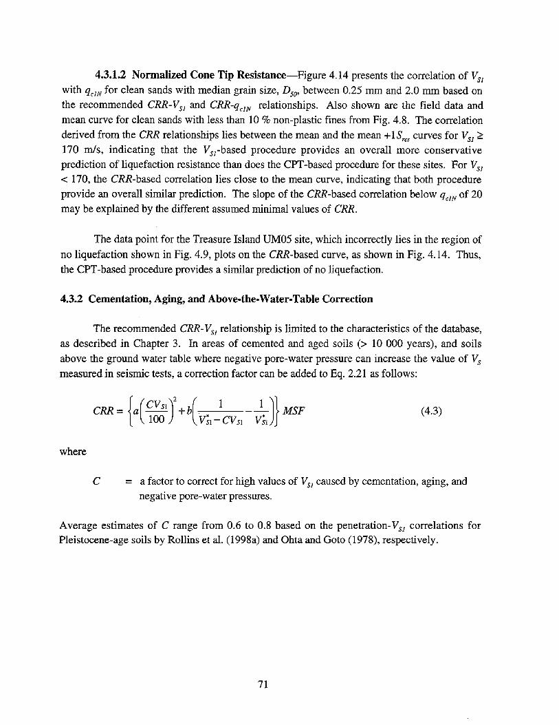
4.3.1.2 Normalized Cone Tip Resistance-Figure 4.14 presents the correlation of VS1with qcIN for clean sands with median grain size, Dso' between 0.25 mm and 2.0 mm based onthe recommended CRR-Vs1 and CRR-qcIN relationships. Also shown are the field data andmean curve for clean sands with less than 10 % non-plastic fines from Fig. 4.8. The correlation
derived from the CRR relationships lies between the mean and the mean +lSres curves for VS1 ~170 mis, indicating that the Vsl-based procedure provides an overall more conservativeprediction of liquefaction resistance than does the CPT-based procedure for these sites. For VS1< 170, the CRR-based correlation lies close to the mean curve, indicating that both procedureprovide an overall similar prediction. The slope of the CRR-based correlation below qcIN of 20may be explained by the different assumed minimal values of CRR.
The data point for the Treasure Island UM05 site, which incorrectly lies in the region of
no liquefaction shown in Fig. 4.9, plots on the CRR-based curve, as shown in Fig. 4.14. Thus,the CPT-based procedure provides a similar prediction of no liquefaction.
4.3.2 Cementation, Aging, and Above-the-Water-Table Correction
The recommended CRR-VS1 relationship is limited to the characteristics of the database,as described in Chapter 3. In areas of cemented and aged soils (> 10 000 years), and soilsabove the ground water table where negative pore-water pressure can increase the value of Vsmeasured in seismic tests, a correction factor can be added to Eq. 2.21 as follows:
where
{( ) 2 ( )}CRR = a CVs1 +b. 1 __1_ MSF100 V~l - CVSl V~l
(4.3)
C = a factor to correct for high values of VS1 caused by cementation, aging, andnegative pore-water pressures.
Average estimates of C range from 0.6 to 0.8 based on the penetration-VS1 correlations forPleistocene-age soils by Rollins et al. (1998a) and Ohta and Goto (1978), respectively.
71
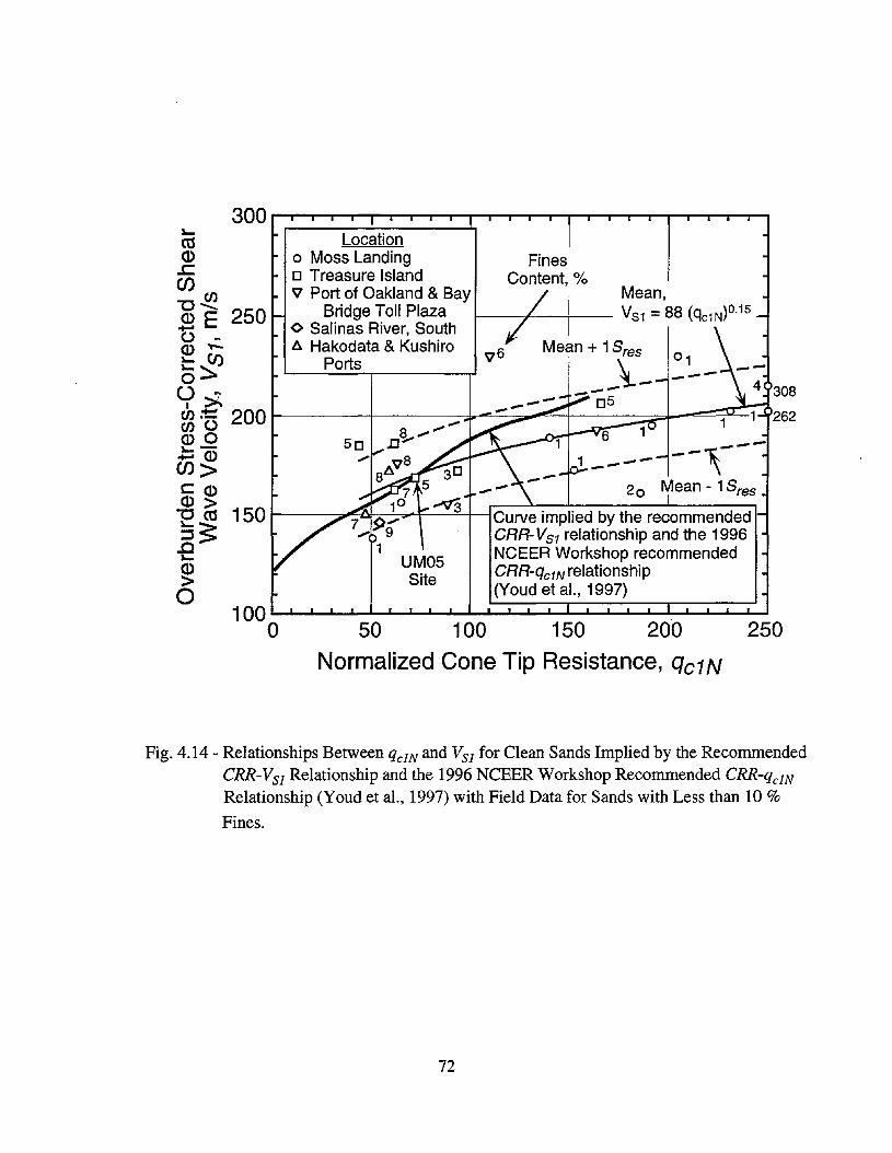
Locationo Moss Landing Fineso Treasure Island Content, %v Port of Oakland & Bay Mean,
Bridge Toll Plaza I----/--+--- VS1 =88 (QC1N)O.15
<> Salinas River, Southti. Hakodata & Kushiro
Ports
lIo..
ctS(1)..cen"'C~(1) E 250+J
o (1)"""
~~O~ ~en;t: 200 1--------l------d........,..~~~+_~-=-___=d.-~~::1~262cnO(1)0
O)~ --,---C (1) 20 Mean - 1Sres~?= 150 '---_---:.i~Iif_=_==___T__--=-+---I.--------J...-...l.------l------.~ :> .- Curve implied by the recommended_ > CRR-VS1 relationship and the 1996-e NCEER Workshop recommended~ CRR-%1N relationshipo (Youd et aI., 1997)
100 L....-L.....L-...L.-..I--'-...L-L-L........L-.I-..I.--I......L.".,.lL.....L..-I-.L.....L.--I.....I......I--.L.-I-..I......I
o 50 100 150 200 250
Normalized Cone Tip Resistance, Qc1N
Fig. 4.14 - Relationships Between qclN and VS1 for Clean Sands Implied by the RecommendedCRR-VS1 Relationship and the 1996 NCEER Workshop Recommended CRR-qclNRelationship (Youd et aI., 1997) with Field Data for Sands with Less than 10 %
Fines.
72

Figures 4.15 and 4.16 illustrate a method for estimating the value of C using SPT andCPT test results, respectively. Shown in the figures are the VSj-penetration correlation curvesfor clean soils and silty soils implied by the recommended CRR-VSj relationship and the 1996NCEER workshop recommended CRR-penetration relationships (Youd et aI., 1997). In the
example, the measured values of VSj' (Nj)60' qcJN' and fines content are 220 mis, 8, 55, and10 %, respectively. The VSj-penetration correlation curves suggest a C value of 0.74 for theseconditions.
The method for estimating C described above assumes that the strain level inducedduring penetration testing is the same strain level causing liquefaction. This may not be true
since pore-water pressure buildup to liquefaction can occur at medium strains in several loadingcycles (Dobry et aI., 1982; Seed et al., 1983).
4.3.3 High Overburden Stress Correction
To adjust cyclic resistance ratios where overburden stresses are much greater than100 kPa, Seed (1983) developed the correction factor Kcr This correction is applied by:
(4.4)
where
CRRj = the cyclic resistance ratio at the reference overburden stress (100 kPa).
The original correction factors were derived from isotropically consolidated cyclictriaxial compression test results. They decreased almost linearly with effective overburdenpressure from a value of 1.0 at 100 kPa to values ranging from 0.4 to 0.65 at 800 kPa.Modifications to these factors have been suggested based on subsequent analyses of additionalcyclic triaxial and constant-volume cyclic simple shear tests (Vaid et aI., 1985; Seed andHarder, 1990; Pillai and Byrne, 1994; Vaid and Thomas, 1995; Arango, 1996), as shown in Fig.4.17. Figure 4.18 presents the relationship of minimal values of Ka recommended by the 1996NCEER workshop (Youd et al., 1997; Harder and Boulanger, 1997) for both sands and gravels.
Hynes and Olsen (1998) compiled and examined a database of about 150 Ka values forgravels, sands and silt-sand mixtures at densities ranging from very loose to very dense. Thedatabase consisted of both undisturbed and reconstituted specimens. The reconstitutedspecimens were pluviated through air, pluviated through water, and constructed in layers bymoist tamping or vibration. Hynes and Olsen compared the laboratory estimates of eRR at one
73

50
< 5% Fines
Example result of in situ testsfor weakly cemented soil with10 % non-plastic fines.
C= 162/220 = 0.74
10 20 30 40
Corrected Blow Count, (Nt)60
VS1 =220 rnIs---....
I
250 t------+----::~
200 ~----l-+-----l=.__=---+----+-----1
Curves implied by the150 1--7~-'!-'f-J-+-----+---4recommended CRR-VS1
relationship and the 1996NCEER Workshoprecommended CRR-(N1)60
relationship (Youd et aI., 1997)
J...
mCD
..cen-e~CDE.....o CD"""
~~o -.>-en.:'!:enOCDOJ...-..... CDen>CCDCD>-em~S..cJ...
CD>o
Fig. 4.15 - Relationships Between (Nj )60 and VSj Implied by the Recommended CRR-VSj
Relationship and the 1996 NCEER Workshop Recommended CRR-(Nj )60
Relationship (Youd et aI., 1997) with an Example for Determining theCorrection Factor C at a Weakly Cemented Soil Site.
74

< 5 % Fines10 ~~ ..
Example result of in situ testsfor weakly cemented soil with10 % non-plastic fines.
C = 163/220 = 0.74
VS1 = 220 m/s
~
ctSCD.c(J)
"O~CD E 250 1-----+---+-1+-'U -(]).,...
~~Y>.en .'t: 200 ~---r-+-+-----t-~-=;;;;"-""""""--t------t----'------IenU I(])O I~ CD I I(J» I I •• ••
a5 (]» -,T - - -= .' VS1 = 163 m/s Curves implied by the-,..oc - 150- \,u. recommended CRR-VS1~> I_ > , .... relationship and the 1996-e I NCEER Workshop~ : recommended CRR-qc1No IQc1N= 55' relationship (Youd et aI., 1997)
100 ...........--L-...r........I.........I..I-.a.--.&.--I--'---IL.-...L..............I..--&--I--L.....&...-..l.--L-..L-...........--'---I
o 50 100 150 200 250
Normalized Cone Tip Resistance, Qc1N
Fig. 4.16 - Relationships Between qc1N and VS1 Implied by the Recommended CRR-VsRelationship and the 1996 NCEER Workshop Recommended CRR-Qc1NRelationship (Youd et aI., 1997) with an Example for Determining theCorrection Factor C at a Weakly Cemented Soil Site.
75
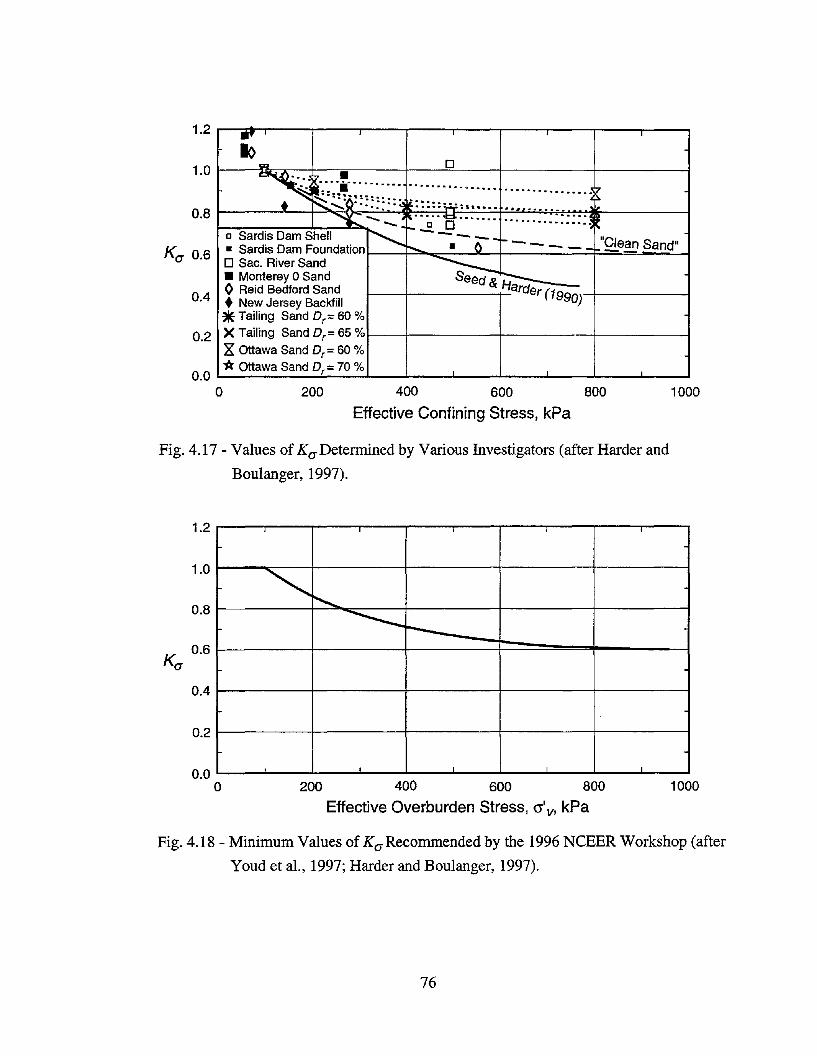
1000400 600 800
Effective Confining Stress, kPa200
...10
"'" 0
~ '·.··1·········.. .................... ................~• ~:::6~··::··~~ lL::::::,.:.:: •••......... ..... :.. ... .......
~--'~ .....~ ....... ...... ~
~~~ 0...............,
D Sardis Dam Shell ~ -------1-_- "Q!.ean Sand"• Sardis Dam Foundation r-.... • 6 ---o Sac. River Sand ~• Monterey 0 Sand Seed & Ho Reid Bedford Sand arder (1990;• New Jersey Backfill.. Tailing Sand Dr= 60 %X Tailing Sand Dr= 65 %X Ottawa Sand Dr= 60 %'* Ottawa Sand Dr= 70 %
0.2
0.0o
0.8
0.4
1.0
1.2
Fig. 4.17 - Values of K(J'Determined by Various Investigators (after Harder and
Boulanger, 1997).
1.2
1.0
0.8
K 0.6(J'
'"~ -----------0.4
0.2
0.0o 200 400 600 800
Effective Overburden Stress, cr'v, kPa1000
Fig. 4.18 - Minimum Values of K(J'Recommended by the 1996 NCEER Workshop (after
Youd et aI., 1997; Harder and Boulanger, 1997).
76
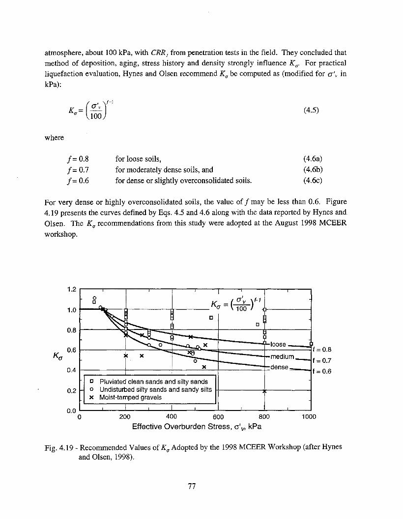
atmosphere, about 100 kPa, with eRR1 from penetration tests in the field. They concluded thatmethod of deposition, aging, stress history and density strongly influence K(J. For practicalliquefaction evaluation, Hynes and Olsen recommend K(J be computed as (modified for a'v inkPa):
(4.5)
where
1=0.81=0.71=0.6
for loose soils,
for moderately dense soils, and
for dense or slightly overconsolidated soils.
(4.6a)
(4.6b)
(4.6c)
For very dense or highly overconsolidated soils, the value of1 may be less than 0.6. Figure4.19 presents the curves defined by Eqs. 4.5 and 4.6 along with the data reported by Hynes andOlsen. The K(J recommendations from this study were adopted at the August 1998 MCEER
workshop.
f= 0.8
f= 0.7
f =0.6
1000200 400 600 800
Effective Overburden Stress, cr'v, kPa
I0
K = (a'v )'-1[]n_
(J 100
~[] ~
~ I []
....
~~
~ .... x J, loose-~x -medium_0
x -dense
[] Pluviated clean sands and silty sands0 Undisturbed silty sands and sandy siltsx Moist-tamped gravels
I I
0.8
0.2
0.0o
0.4
0.6K(J
1.2
1.0
Fig. 4.19 - Recommended Values of K(J Adopted by the 1998 MCEER Workshop (after Hynesand Olsen, 1998).
77

78

CHAPTERS
APPLICATION OF THE PROCEDURE FOR EVALUATING
LIQUEFACTION RESISTANCE
5.1 PROCEDURE SUMMARY
The procedure for evaluating liquefaction resistance outlined in the previous chapters issummarized in the following steps:
1. From available subsurface data, develop detailed profiles of shear wavevelocity, soil type, fines content (particles less than 75 ~m), and, if possible,soil density and penetration resistance.
2. Identify the depth of the ground water table, noting any seasonal fluctuationsand artesian pressures.
3. Calculate the total and effective overburden stresses for each measurementdepth at which seismic testing has been performed.
4. Correct the shear wave velocity measurements to the reference overburdenstress of 100 kPa, as shown in Eq. 3.2.
5. Determine the limiting upper value of overburden stress-corrected shearwave velocity for liquefaction occurrence, ~I' for each measurement depthusing Eq. 4.1. If the fines content is unknown, assume 215 rnIs for ~I'
6. Determine the value of the correction factor C. The value of C can beassumed equal to 1, if the soil to be evaluated is uncemented, less than10 000 years old, and lies below the ground water table when the seismictests were conducted. If the soil is cemented, more than 10 000 years, or liesabove the water table, the value of C may be estimated by the methoddescribed in Section 4.3.2. If the soil conditions are unknown andpenetration data are not available, assume 0.6 for C.
79

7. Determine the design earthquake magnitude and the expected peak horizontalground surface acceleration.
8. For each measurement depth below the water table, calculate the cyclic stress
ratio, as shown in Eq. 3.1. The stress reduction coefficient is estimated using
Fig. 2.1.
9. Plot values of VS1 and CSR, and the appropriate liquefaction resistance curvesusing Eqs. 2.13 and 4.3 with a = 0.022, b = 2.8, and n = -2.56. If theeffective overburden stress is greater than 100 kPa, correct curves using Eqs.4.5 and 4.6. Liquefaction is predicted at the site if the data points plot to theleft of the respective liquefaction resistance curve. No liquefaction is
predicted if the data points plot to the right of the respective curve.
A common way to quantify the potential or hazard for liquefaction is in terms of afactor of safety. The factor of safety, FS, against liquefaction can be defined by:
FS= CRRCSR
(5.1)
Liquefaction is predicted to occur when FS is less than 1. When FS is greater than 1,liquefaction is predicted not to occur. The acceptable value of FS will depend on severalfactors including: (1) the acceptable level of risk for the project, (2) the extent and accuracy ofseismic measurements, (3) the availability of other site information, and (4) the conservatism indetermining the design earthquake magnitude and the expected peak ground acceleration.
Thus, the following step may be added to the nine-step procedure give above--
10. Calculate the value of FS for each measurement depth using Eq. 5.1.
5.2 CASE STUDIES
To illustrate the application of the procedure, two sites shaken by the 1989 Lorna Prieta,California, earthquake (Mw =7) are considered below. The two sites are Treasure Island FireStation and Marina District School. These sites are discussed earlier to illustrate how values ofVS1 and CSR are determined (see Section 3.2).
80
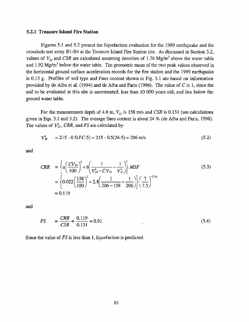
5.2.1 Treasure Island Fire Station
Figures 5.1 and 5.2 present the liquefaction evaluation for the 1989 earthquake and thecrosshole test array B1-B4 at the Treasure Island Fire Station site. As discussed in Section 3.2,values of VS1 and CSR are calculated assuming densities of 1.76 Mg/m3 above the water table
and 1.92 Mg/m3 below the water table. The geometric mean of the two peak values observed inthe horizontal ground surface acceleration records for the fire station and the 1989 earthquake
is 0.13 g. Profiles of soil type and fines content shown in Fig. 5.1 are based on information
provided by de Alba et al. (1994) and de Alba and Faris (1996). The value of C is 1, since the
soil to be evaluated at this site is uncemented, less than 10 000 years old, and lies below the
ground water table.
For the measurement depth of 4.6 m, VS1 is 158 m1s and CSR is 0.131 (see calculationsgiven in Eqs. 3.1 and 3.2). The average fines content is about 24 % (de Alba and Faris, 1996).
The values of lTsl' CRR, and FS are calculated by:
lTsl = 215 - 0.5(FC-5) = 215 - 0.5(24-5) = 206 m1s (5.2)
and
{( )' ( )}CRR = a CVSl +b 1 __1_ MSF (5.3)100 V;I-CVS1 V;l{ ( )' ( )}( r~- 0 022 158 + 2 8 1 __1_ .l-
-. 100 . 206-158 206 7.5
=0.119
and
FS = CRR = 0.119 = 0.91 (5.4)CSR 0.131
Since the value of FS is less than 1, liquefaction is predicted.
81

2
Factor of Safety,FS1
ay bonefiabynesteri
1989 Lorna Prieta Earthquake, Mw=7Cyclic Stress or
Resistance Ratio,CSRorCRR
60 0.0 0.2 0.4 0
FinesContent, %
30
.I I IAverage_values ,
used for_ •analysis ....L{~R-""",If
V ~ •I.
• .~~CSR-• •
Ie M• I
• 0 Iiqu
Ct
ItCI
•It •
)
0
62 IeII Non-liquefiable clay by Chinese criteria I
o
SoilProfile
Siltysand
fill(possiblydumped)
Siltysand fill
(hydraulic)------
Clayeysand
------Silty
sand fill(hydraulic)
Clayeysand
Clay
•....1-r-water •table •
••
It Critical
• Layerv
••
•Soil profile
• and finesCrosshole contentdata for • data fromboreholes • de Alba et81 & 84 • al. (1994),from and de AlbaFuhriman • and Faris(1993) (1996).
I
Overburden Stress-Corrected ShearWave Velocity, VS1, m/s
50 100 150 200 250 300o
15
5
E00tv .c:a.
Q)
0
10
Fig. 5.1 - Application of the Recommended Procedure to the Treasure Island Fire Sation Site, Crosshole Test Array B1-B4 (Depthof 1.5 m to 14 m).

NoLiquefaction
7+-AverageFinesContent (%)
Mw =7
III
~35 20::;5 FinesI I Content (%)
II'
Fines ContentA 6 to 34 %o ~35%
100 200 300
Overburden Stress-Corrected Shear WaveVelocity, VS1, mls
Liquefaction
Chart Based on:Average values of
VS1and 8maxUncemented,
Holocene-age soils
0.0 L.---__..I.-__...I-__--&...__-J..__---J__.---J
o
0.21-------..+--------.14-/--4---------1
cr: 0.6cr:()
~
aca 0.4a:CD(,)Cco+-'enenCDa:L-
aenen~+-'en(,)
(,)>.o
Fig. 5.2 - Recommended Liquefaction Assessment Chart for Magnitude 7 Earthquakeswith Data for the 1989 Lorna Prieta Earthquake and the Treasure Island FireStation Site, Crosshole Test Array BI-B4 (Depths of 1.5 m to 14 m). Since noSurface Manifestations of Liquefaction Occurred at the Site During theEarthquake, the Data Shown are for a Non-liquefaction Case History.
83

Figure 5.1 shows the values of VSj ' CSR, CRR, and FS for crosshole test array B 1-B4 atthe measurement depths below the water table. Values of FS are less than 1 for the depths of 4m to about 9 m. Between the depths of 4 m and 7 m, the sand contains non-plastic fines and isconsidered liquefiable by the Chinese criteria (see Section 1.1). Between the depths of7 m and
9 m, the soil e~hibits plastic characteristics and may be non-liquefiable by the Chinese criteria.
Thus, the plotted values of CRR and FS for this clayey sand layer are shown as open circles.
The layer most likely to liquefy, or the critical layer, lies between the depths of 4 m and 7 m.
Figures 5.3 and 5.4 present the liquefaction evaluation for the SASW test array.Locations of Vs measurements for the SASW test array are assumed at the center of the layerused in forward modeling of surface wave measurements. Values of FS are less than 1 betweenthe depths of about 3.5 m and 11 m. The lowest values of FS in the non-plastic soil is 0.75 at adepth of 5.3 m. This FS value is similar to the lowest FS value of 0.77 determined from
crosshole measurements in the critical layer.
Although no sand boils or ground cracks occurred at the fire station during the 1989earthquake, the prediction of liquefaction agrees with the conclusion stated in Section 3.2.1 thatliquefaction of an underlying sand cause the sudden drop in the acceleration time historiesrecorded at this site (de Alba et aI., 1994). It is possible that the 4 m thick layer capping the
site, predicted not to liquefy (see Figs. 5.1 and 5.3), prevented the formation of sand boils at theground surface (Ishihara, 1985).
5.2.2 Marina District School
Figures 5.5 and 5.6 present the liquefaction evaluation for the Marina District Schoolsite and the 1989 Lorna Prieta earthquake. Values of VSj and CSR are calculated assumingdensities of 1.76 Mg/m3 above the water table and 1.92 Mg/m3 below the water table, asdescribed in Section 3.2.3. They are plotted in Fig. 5.5 at the depths midway between receiverlocations. The profiles of soil type and fines content shown in Fig. 5.5 are based oninformation provided by Kayen et aI. (1990). The upper 7.6 m of soil at the site consists ofsand with 1 % to 8 % fines. Since the sand is uncemented, less than 10 000 years old, and lies
below the ground water table, the value of Cis 1.
Calculated values of FS are 0.42,0.90, and 0.51 at the depths of 3 m, 4 m, and 6.7 m.The clean sand is underlain by a silty clay layer, which is non-liquefiable by the Chinesecriteria (see Section 1.1). Having the lowest average value of FS, the sand fill just below thewater table between the depths of 2.7 m and 4.4 m is identified as the critical layer that
liquefied. A prediction of liquefaction agrees with the observed field behavior.
84

2
Factor of Safety,FS1
seia
be
able
•
•
0
1989 Lorna Prieta Earthquake, Mw = 7Cyclic Stress or
Resistance Ratio,CSRorCRR
60 0.0 0.2 0.4 0
FinesContent, %
30I I I II
Averagevalues - ,
used for_analysis ~ ""'> CRR1
V ~ i/,
t tk- I,--CSR-••
• ("- May
K nor....... Iiquefi
t / b)Chin,
7 crite
•IJ
~2
IINon-liquefiable clay by Chinese criteria I
o
SoilProfile
Siltysand
fill(possiblydumped)
Siltysand fill
(hydraulic)------
Clayeysand
------Silty
sand fill(hydraulic)
Clayeysand
Clay
~ -I-watertable •
.../
/' - Critical-Data points Layerplotted at
-center oflayer used
-in SASW •forward-modeling
Soil profileand finescontentdata from
Unpublished de Alba etSASW data • al. (1994),by The Univ. and de Albaof Texas at and FarisAustin (1996).
I
Overburden Stress-Corrected ShearWave Velocity, VS1, mls
50 100 150 200 250 300o
15
5
00 EVI ..c-C-
Q)
0
10
Fig. 5.3 - Application of the Recommended Procedure to the Treasure Island Fire Sation Site, SASW Test Array (Depths of 2 m to13 m).

100 200 300Overburden Stress-Corrected Shear Wave
Velocity, VS1, m/s
Mw=7
NoLiquefaction
AverageFinesContent (%)
III
~35 20 $;5 Fines, I Content (%)
III
Liquefaction
Fines Content~ 6 to 34 %o ~35%
Chart based on:Average values of
VS1and 8maxUncemented,
Holocene-age soils
a: 0.6 r---~----,-----r----,----~----.,a:()
~
oca 0.4ex:Q)()c~-enenQ)
ex:J... 0.2 t--------+-------,f-+-j'-+------~oenen~-C/)()
()>.() 0.0 100.-__.1.....-__.1.....-__..10-__..10-__...1..-_-----'
o
Fig. 5.4 - Recommended Liquefaction Assessment Chart for Magnitude 7 Earthquakeswith Data for the 1989 Lorna Prieta Earthquake and the Treasure Island FireStation Site, SASW Test Array (Depths of 2 m to 13 m). Since no SurfaceManifestations of Liquefaction Occurred at the Site During the Earthquake,the Data Shown are for a Non-liquefaction Case History.
86

Factor of Safety,FS
012'I I
FS= CRR'-- CSR I-
.....
IVery high,l 4
VS1> VS1 T
•
IVery high, .1VS 1 > VS1*
1989 Lorna Prieta Earthquake, Mw= 7Cyclic Stress or
Resistance Ratio,CSRorCRR
60 0.0 0.2 0.4
FinesContent, %
30CT
Average
i~values
used for~ analysis
./I#'
..~ CtR
1-- F.;7CRR
..",V•I)
100 cI--~Non-liquefiable clay by Chinese criteria L-
0/
o
SoilProfile
Sandfill
(hydraulicor
dumped)
Naturalsand
(possiblydune orbeach)
Naturalsilty clay
(HoloceneBay Mud)
Data pOi~ts plotte~midway betweenreceiver locations
water ~-table
./ •-L
Critical
• Layer
•
••
•Velocity and soil data
• from Kayen et al.(1990); velocitiesrecalculated by pseudo-
• interval methodI I
8
2
Overburden Stress-Corrected ShearWave Velocity, VS1, mls
50 100 150 200 250 300o
10
400 E.......:J .r=.....
0.Q)
06
Fig. 5.5 - Application of the Recommended Procedure to the Marina District School Site (Depths of 3 m to 10 m).

o
NoLiquefaction
III
Mw=7~35 20:::;5 Fines
, I Content (%)
III
oo
Liquefaction
Fines Contento <5%
100 200 300Overburden Stress-Corrected Shear Wave
Velocity, VS1, mls
Chart based on:Average values of
VS1and amaxUncemented,
Holocene-age soils
0.0 "--__...a.-__--'--__.......I-__---'- "'--_----.-I
o
0.2 t--------+-----++-.f-+-------I
0: 0.6 r---r------,----r----,------,..-----,
0:o
~
oenenCD~
+-'en(.)
(.)~
(,)
~
o0:
~o1ti 0.40:CD(.)CctS+-'enenCD0:
Fig. 5.6 - Recommended Liquefaction Assessment Chart for Magnitude 7 Earthquakeswith Data for the 1989 Lorna Prieta Earthquake and the Marina District SchoolSite (Depths of 3 m to 7 m). Since Surface Manifestations of LiquefactionOccurred Near the Site During the Earthquake, the Data Shown are for aLiquefaction Case History.
88

CHAPTER 6
SUMMARY AND RECOMMENDATIONS
6.1 SUMMARY
Presented in this report are draft guidelines for evaluating liquefactiori resistance
through shear wave velocity, Vs, measurements. The guidelines were written in cooperationwith industry, researchers and practitioners, and evolved from workshops held in 1996 and1998. They include the development of a recommended procedure and guidance for its use.
The recommended procedure follows the general format of the simplified penetrationbased procedure originally proposed by Seed and Idriss (1971). Cyclic stress ratios, CSR, arecalculated using Eq. 2.1, with the average stress reduction coefficient estimated from Fig. 2.1.Vs measurements are corrected for overburden stress using Eq. 2.7. The ten main steps forapplying the recommended procedure are summarized in Section 5.1.
Liquefaction resistance curves are based on a modified relationship between overburdenstress-corrected shear wave velocity, VSJ ' and cyclic stress ratio for constant average cyclicshear strain suggested by R. Dobry (personal communication to R. D. Andrus, 1996). Thequadratic relationship proposed by Dobry is modified so that it is asymptotic to some limitingupper value of VSJ • This limit is related to the tendency of dense granular soils to exhibitdilative behavior at large strains, as well as the fact that dense soils expel dramatically lesswater during reconsolidation than loose soils. The modified relationship is given by Eq. 2.21.To determine the unknown parameters of Eq. 2.21, liquefaction and non-liquefaction casehistories from 26 earthquakes and more than 70 measurement sites in soils ranging from cleanfine sand to sandy gravel with cobbles to profiles including silty clay layers are analyzed.Penetration-Vs correlations are also considered.
Figures 4.1 through 4.6 present the recommended evaluation curves for uncemented,Holocene-age soils and different earthquake magnitudes. These curves are defined by Eqs.2.13 and 2.21 with a =0.022, b =2.8, ~l =200 m/s to 215 m/s (depending on fines content),and n =-2.56. These values were selected such that the evaluation curves bounded over 95 %
89
of the case histories where liquefaction occurred. By constructing relationships between VS1
and penetration resistance from the recommended evaluation curves and plotting available insitu test data, it was shown that the VsFbased evaluation curves are generally more conservativethan the penetration-based evaluation curves. Corrections are suggested for cemented and aged
soils, as well as high overburden stress conditions, in Sections 4.3.2 and 4.3.3.
Caution should be exercised when applying the procedure to sites where conditions aredifferent from the database. The case history data are limited to relatively level ground siteswith the following general characteristics: (1) uncemented soils of Holocene age; (2) averagedepths less than about 10 m; and (3) ground water table depths between 0.5 m and 6 m. All Vsmeasurements are from below the water table. About three-quarters of the case history data arefor soils with fines content greater than 5 %. Almost half of the case histories are forearthquakes with magnitudes near 7.
Three concerns when using shear wave velocity as an indicator of liquefactionresistance are (1) its higher sensitivity (when compared with the penetration-based methods) toweak interparticle bonding, (2) the lack of a physical sample for identifying non-liquefiableclayey soils, and (3) not detecting thin liquefiable strata because the test interval is too large.The preferred practice is to drill sufficient boreholes and conduct sufficient other in situ tests todetect thin liquefiable strata, to identify non-liquefiable clay-rich soils, to identify silty soilsabove the ground water table that might have lower values of Vs should the water table rise, andto detect liquefiable weakly cemented soils.
6.2 FUTURE STUDIES
The following future studies are recommended:
1. Additional well-documented case histories with all types of soil that have and havenot liquefied during earthquakes should be compiled, particularly from deeper deposits (depth >8 m) and from denser soils (Vs > 200 m/s) shaken by stronger ground motions (amax > 0.4 g), tofurther validate the recommended curves. Also, case histories from lower magnitudeearthquakes (Mw < 7) may improve estimates of the magnitude scaling factor.
2. Laboratory and field studies should be conducted to further refine estimates of ~l'
the limiting value of VS1 for liquefaction occurrence. For example, careful laboratory studiesmay identify more clearly the influence of fines content and particle size on V~l. Additionalcareful penetration-Vs correlation studies may also help refine the ~l estimates.
90

3. Laboratory studies should also be conducted to evaluate the implied assumptionobserved in Fig. 4.9 that at low values of VSJ (say 100 m1s) liquefaction resistance isindependent of fines content.
4. Additional work is needed to evaluate the significance of ignoring soil type andhorizontal stress in the overburden correction.
5. Standard test procedures exist only for the crosshole test. Standard test methodsshould be developed for the other in situ seismic tests.
91

92

REFERENCES
Abdel-Haq, A., and Hryciw, R. D. (1998). "Ground Settlement in Simi Valley Following theNorthridge Earthquake," Journal of Geotechnical and Geoenvironmental Engineering, ASCE,Vol. 124, No.1, pp. 80-89.
Ambraseys, N. N. (1988). "Engineering Seismology," Earthquake Engineering and StructuralDynamics, Vol. 17, p. 1-105.
American Society of Testing and Materials, ASTM, D-4428M-91. "Standard Test Methods forCrosshole Seismic Testing," Annual Book ofASTM Standards, Vol. 4.08.
Andrus, R. D. (1994). "In Situ Characterization of Gravelly Soils That Liquefied in the 1983Borah Peak Earthquake," Ph.D. Dissertation, The University of Texas at Austin, 533 p.
Andrus, R. D., and Stokoe, K. H., II (1997). "Liquefaction Resistance Based on Shear WaveVelocity," NCEER Workshop on Evaluation of Liquefaction Resistance of Soils, TechnicalReport NCEER-97-0022, T. L. Youd and 1. M. Idriss, Eds., held 4-5 January 1996, Salt LakeCity, UT, National Center for Earthquake Engineering Research, Buffalo, NY, pp. 89-128.
Andrus, R. D., Stokoe, K. H., II, Bay, J. A., and Chung, R. M. (1998a). "Delineation ofDensified Sand at Treasure Island by SASW Testing," Geotechnical Site Characterization, P.K. Robertson and P. W. Mayne, Eds., A. A. Balkema, Rotterdam, Netherlands, pp. 459-464.
Andrus, R. D., Stokoe, K. H., II, Chung, R. M., and Bay, J. A. (1998b). "LiquefactionEvaluation of Densified Sand at Approach to Pier 1 on Treasure Island, California, UsingSASW Method," NISTIR 6230, National Institute of Standards and Technology, Gaithersburg,MD, 75 p.
Andrus, R. D., Stokoe, K. H., II, Bay, J. A., and Youd, T. L. (1992). "In Situ Vs of GravellySoils Which Liquefied," Proceedings, Tenth World Conference on Earthquake Engineering,held 19-24 July 1992, Mardrid, Spain, A. A. Balkema, Rotterdam, Netherlands, pp. 1447-1452.
Andrus, R. D., and Youd, T. L. (1987). "Subsurface Investigation of a Liquefaction-InducedLateral Spread, Thousand Springs Valley, Idaho," Geotechnical Laboratory MiscellaneousPaper GL-87-8, U.S. Army Engineer Waterways Experiment Station, Vicksburg, MS, 131 p.
Arango, 1. (1996). "Magnitude Scaling Factors for Soil Liquefaction Evaluations," Journal ofGeotechnical Engineering, ASCE, Vol. 122, No. 11, pp. 929-936.
93

Arulanandan, K., Yogachandran, C., Meegoda, N. J., Ying, L., and Zhauji, S. (1986)."Comparison of the SPT, CPT, SV and Electrical Methods of Evaluating Earthquake InducedLiquefaction Susceptibility in Ying Kou City During the Haicheng Earthquake," Use of In SituTests in Geotechnical Engineering, Geotechnical Special Publication No.6, S. P. Clemence,Ed., ASCE, pp. 389-415.
Barrow, B. L. (1983). "Field Investigation of Liquefaction Sites in Northern California,"Geotechnical Engineering Thesis GT83-1, The University of Texas at Austin, 213 p.
Bennett, M. J., Youd, T. L., Harp, E. L., and Wieczorek, G. F. (1981). "SubsurfaceInvestigation of Liquefaction, Imperial Valley Earthquake, California, October 15, 1979,"Open-File Report 81-502, U.S. Geological Survey, Menlo Park, CA, 83 p.
Bennett, M. J., McLaughlin, P. V., Sarmiento, J. S., and Youd, T. L. (1984). "GeotechnicalInvestigation of Liquefaction Sites, Imperial Valley, California," Open-File Report 84-252,U.S. Geological Survey, Menlo Park, CA, 103 p.
Bennett, M. J., and Tinsley, J. C. (1995). "Geotechnical Data from Surface and SubsurfaceSamples Outside of and within Liquefaction-Related Ground Failures Caused by the October17, 1989, Lorna Prieta Earthquake, Santa Cruz and Monterey Counties, California," Open-FileReport 95-663, U.S. Geological Survey, Menlo Park, CA.
Bierschwale, J. G., and Stokoe, K. H., II (1984). "Analytical Evaluation of LiquefactionPotential of Sands Subjected to the 1981 Westmorland Earthquake," Geotechnical EngineeringReport GR-84-15, The University of Texas at Austin, 231 p.
Boulanger, R. W., Idriss, I. M., and Mejia, L. H. (1995). "Investigation and Evaluation ofLiquefaction Related Ground Displacements at Moss Landing During the 1989 Lorna PrietaEarthquake," Report No. UCD/CGM-95/02, University of California at Davis.
Boulanger, R. W., Mejia, L. H., and Idriss, I. M. (1997). "Liquefaction at Moss LandingDuring Lorna Prieta Earthquake," Journal of Geotechnical and Geoenviromental Engineering,ASCE, Vol. 123, No.5, pp. 453-467.
Brady, A. G., and Shakal, A. F. (1994). "Strong-Motion Recordings," The Lorna Prieta,California, Earthquake of October 17, 1989--Strong Ground Motion, U.S. Geological SurveyProfessional Paper 1551-A, R. D. Borcherdt, Ed., U.S. Gov. Printing Office, Washington, D.C.,pp. A9-A38.
de Alba, P., Baldwin, K., Janoo, V., Roe, G., and Celikkol, B. (1984). "Elastic-WaveVelocities and Liquefaction Potential," Geotechnical Testing Journal, ASTM, Vol. 7, No.2,pp.77-87.
94

de Alba, P., Benoit, J., Pass, D. G., Carter, J. J., Youd, T. L., and Shakal, A. F. (1994). "DeepInstrumentation Array at the Treasure Island Naval Station," The Loma Prieta, California,Earthquake of October 17, 1989--Strong Ground Motion, U.S. Geological Survey ProfessionalPaper 1551-A, R. D. Borcherdt, Ed., U.S. Gov. Printing Office, Washington, D.C., pp. A155A168.
de Alba, P., and Faris, J. R. (1996). "Workshop on Future Research Deep InstrumentationArray, Treasure Island NGES, July 27, 1996: Report to the Workshop Current State of SiteCharacterization and Instrumentation," University of New Hampshire at Durham, 45 p.
Dobry, R. (1989). "Some Basic Aspects of Soil Liquefaction during Earthquakes," EarthquakeHazards and the Design of Constructed Facilities in the Eastern United States, K. H. Jacob andC. 1. Turkstra, Eds., New York Academy of Sciences, Vol. 558, pp. 172-182.
Dobry, R., and Ladd, R. S. (1980). Discussion to "Soil Liquefaction and Cyclic MobilityEvaluation for Level Ground During Earthquakes," by. H. B. Seed and "Liquefaction Potential:Science versus Practice," by R. B. Peck, Journal of the Geotechnical Engineering Division,ASCE, Vol. 106, GT. 6, pp. 720-724.
Dobry, R., Ladd, R. S., Yokel, F. Y., Chung, R. M., Powell, D. (1982). "Prediction of PoreWater Pressure Buildup and Liquefaction of Sands During Earthquakes by the Cyclic StrainMethod," NBS Building Science Series 138, National Bureau of Standards, Gaithersburg, MD,152p.
Dobry, R., Stokoe, K. H., IT, Ladd, R. S., and Youd, T. L. (1981). "Liquefaction Susceptibilityfrom S-Wave Velocity," Proceedings, In Situ Tests to Evaluate Liquefaction Susceptibility,ASCE National Convention, held 27 October 1981, St. Louis, MO.
Dobry, R., Baziar, M. H., O'Rourke, T. D., Roth, B. L., and Youd, T. L. (1992). "Liquefactionand Ground Failure in the Imperial Valley, Southern California During the 1979, 1981 and1987 Earthquakes," Case Studies of Liquefaction and Lifeline Performance During PastEarthquakes, Technical Report NCEER-92-0002, T. O'Rourke and M. Hamada, Eds., NationalCenter for Earthquake Engineering Research, Buffalo, NY, Vol. 2.
Drnevich, V. P., and Richart, F. E., Jr. (1970). "Dynamic Prestraining of Dry Sand," Journal ofthe Soil Mechanics and Foundations Division, ASCE, Vol. 96, No. SM2, pp. 453-469.
EPRI (1992). Lotung Large-Scale Seismic Test Strong Motion Records, EPRI NP-7496L,Electric Power Research Institute, Palo Alto, CA, Vols. 1-7.
Finn, W. D. L., and Bhatia, S. K. (1981). "Prediction of Seismic Pore-water Pressures,"Proceedings, Tenth International Conference on Soil Mechanics and Foundation Engineering,VoL 3, A. A. Balkema Publishers, Rotterdam, Netherlands, pp. 201-206.
Frankel, A., Mueller, c., Barnhard, T., Perkins, D., Leyendecker, E., Dickman, N., Hanson, S.,and Hopper, M. (1996). "National Seismic-Hazard Maps: Documentation," Open-File Report96-532, u.S. Geological Survey, Denver, CO, 110 p.
95

Frankel, A., Mueller, c., Barnhard, T., Perkins, D., Leyendecker, E., Dickman, N., Hanson, S.,and Hopper, M. (1997). "Seismic-Hazard Maps for the Contiguous United States," Open-FileReport 97-131, U.S. Geological Survey, Denver, CO, 12 maps.
Fuhriman, M. D. (1993). "Crosshole Seismic Tests at Two Northern California Sites Affectedby the 1989 Lorna Prieta Earthquake," M.S. Thesis, The University of Texas at Austin, 516 p.
Geomatrix Consultants (1990). "Results of Field Exploration and Laboratory Testing Programfor Perimeter Dike Stability Evaluation Naval Station Treasure Island San Francisco,California," Project No. 1539.05, report prepared for U.S. Navy, Naval Facilities EngineeringCommand, Western Division, San Bruno, CA, Vol. 2.
Gibbs, J. F., Fumal, T. E., Boore, D. M., and Joyner, W. B. (1992). "Seismic Velocities andGeologic Logs from Borehole Measurements at Seven Strong-Motion Stations that Recordedthe Lorna Prieta Earthquake," Open-File Report 92-287, U.S. Geological Survey, Menlo Park,CA,139p.
Golesorkhi, R. (1989). "Factors Influencing the Computational Determination of EarthquakeInduced Shear Stresses in Sandy Soils," Ph.D. Dissertation, University of California atBerkeley, 369 p.
Hanshin Expressway Public Corporation (1998). "The Hanshin Expressway GeologicalDatabase, Volume for Seismic Damage Reconstruction of Route No.3, the Kobe Line, andRoute No.5, the Harbor Line," 224 p. (in Japanese).
Hamada, M., Isoyama, R., and Wakamatsu, K. (1995). The 1995 Hyogoken-Nanbu (Kobe)Earthquake: Liquefaction, Ground Displacement and Soil Condition in Hanshin Area, WasedaUniversity, Tokyo, Japan, 194 p.
Harder, L. F., Jr., and Boulanger, R. (1997). "Application of Kcr and Ka Correction Factors,"NCEER Workshop on Evaluation of Liquefaction Resistance of Soils, Technical ReportNCEER-97-0022, T. L. Youd and I. M. Idriss, Eds., held 4-5 January 1996, Salt Lake City, UT,National Center for Earthquake Engineering Research, Buffalo, NY, pp. 167-190.
Hardin, B. 0., and Drnevich, V. P. (1972). "Shear Modulus and Damping in Soils: DesignEquations and Curves," Journal of the Soil Mechanics and Foundations Division, ASCE, Vol.98, SM7, pp. 667-692.
Heaton, T. H., Tajima, F., and Mori, A. W. (1982). "Estimating Ground Motions UsingRecorded Accelerograms," Report by Dames and Moore to Exxon Production Res. Co.,Houston Texas.
96

Holzer, T. L., Ed. (1998). "Map Showing Locations of Ground-Failures and Damage toFacilities on Treasure Island Attributed to the 1989 Lorna Prieta Earthquake," The Loma Prieta,California Earthquake ofOctober 17, 1989--Liquefaction, U.S. Geological Survey ProfessionalPaper 1551-B, U.S. Gov. Printing Office, Washington, D.C., BI-B8.
Hryciw, R. D. (1991). "Post Lorna Prieta Earthquake CPT, DMT and Shear Wave VelocityInvestigations of Liquefaction Sites in Santa Cruz and on Treasure Island," Final Report to theU.S. Geological Survey, Award No. 14-08-000l-GI865, University of Michigan at Ann Arbor,68 p.
Hryciw, R. D., Rollins, K. M., Homolka, M., Shewbridge, S. E., and McHood, M. (1991)."Soil Amplification at Treasure Island During the Lorna Prieta Earthquake," Proceedings,Second International Conference on Recent Advances in Geotechnical Earthquake Engineeringand Soil Dynamics, S. Prakash, Ed., held 11-15 March 1991, St. Louis, MO, University ofMissouri at Rolla, Vol. II, pp. 1679-1685.
Hryciw, R. D., Shewbridge, S. E., Kropp, A., and Homolka, M. (1998). "PostearthquakeInvestigation at Liquefaction Sites in Santa Cruz and on Treasure Island," The Loma Prieta,California Earthquake ofOctober 17, 1989--Liquefaction, U.S. Geological Survey ProfessionalPaper 1551-B, T. L. Holzer, Ed., U.S. Gov. Printing Office, Washington, D.C., pp. BI65-BI80.
Hynes, M. E. (1988). "Pore Pressure Generation Characteristics of Gravel Under UndraindedCyclic Loading," Ph.D. Dissertation, University of California, Berkeley.
Hynes, M. E., and Olsen, R. S. (1998). "Influence of Confining Stress on LiquefactionResistance," Proceedings, International Workshop on the Physics and Mechanics of SoilLiquefaction, held 10-11 September 1998, Baltimore, MD, A. A. Balkema, Rotterdam,Netherlands.
Iai, S., Morita, T., Kameoka, T., Matsunaga, Y., and Abiko, K. (1995). "Response of a DenseSand Deposit During 1993 Kushiro-Oki Earthquake," Soils and Foundations, Japanese Societyof Soil Mechanics and Foundation Engineering, Vol. 35, No.1, pp. 115-131.
Idriss, I. M. (1990). "Response of Soft Soil Sites During Earthquakes," H. Bolton SeedMemorial Symposium, BiTech Publishers, Vancouver, B.C., Vol. 2, pp. 273-289.
Idriss, I. M. (1991). "Earthquake Ground Motions at Soft Soil Sites," Proceedings, SecondInternational Conference on Recent Advances in Geotechnical Earthquake Engineering andSoil Dynamics, S. Prakash, Ed., held 11-15 March 1991, St. Louis, MO, University of Missouriat Rolla, Vol. ill, pp. 2265-2272.
Idriss, I. M. (1998). "Evaluation of Liquefaction Potential, Consequences and Mitigation--AnUpdate," Presentation notes for Geotechnical Society Meeting, held 17 February 1998,Vancouver, Canada.
97

Idriss, 1. M. (1999). "An Update of the Seed-Idriss Simplified Procedure for EvaluatingLiquefaction Potential," Presentation notes for Transportation Research Board Workshop onNew Approaches to Liquefaction Analysis, held 10 January 1999, Washington, D.C.
Inatomi, T., Zen, K., Toyama, S., Uwabe, T., Iai, S. Sugano, T., Terauchi, K., Yokota, H.,Fujimoto, K.,.Tanaka, S., Yamazaki, H., Koizumi, T., Nagao, T., Nozu, A., Miyata, M., Ichii,K., Morita, T., Minami, K., Oikawa, K., Matsunaga, Y., Ishii, M., Sugiyama, M., Takasaki, N.,Kobayashi, N., and Okashita, K. (1997). "Damage to Port and Port-related Facilities by the1995 Hyogoken-Nanbu Earthquake," Technical Note No. 857, Port and Harbour ResearchInstitute, Yokosuka, Japan, 1762 p.
Ishihara, K. (1985). "Stability of Natural Deposits During Earthquakes," Proceedings,Eleventh International Conference on Soil Mechanics and Foundation Engineering, A. A.Balkema Publishers, Rotterdam, Netherlands, pp. 321-376.
Ishihara, K., Shimizu, K., and Yamada, Y. (1981). "Pore Water Pressures Measured in SandDeposits During an Earthquake," Soils and Foundations, Japanese Society of Soil Mechanicsand Foundation Engineering, Vol. 21, No.4, pp. 85-100.
Ishihara, K., Anazawa, Y., and Kuwano, J. (1987). "Pore Water Pressures and Ground MotionsMonitored During the 1985 Chiba-Ibaragi Earthquake," Soils and Foundations, JapaneseSociety of Soil Mechanics and Foundation Engineering, Vol. 27, No.3, pp. 13-30.
Ishihara, K., Muroi, T., and Towhata, 1. (1989). "In-situ Pore Water Pressures and GroundMotions During the 1987 Chiba-Toho-Oki Earthquake," Soils and Foundations, JapaneseSociety of Soil Mechanics and Foundation Engineering, Vol. 29, No.4, pp.75-90.
Ishihara, K., Karube, T., and Goto, Y. (1997). "Summary of the Degree of Movement ofImproved Masado Reclaimed Land," Proceedings, 24th 1SCE Earthquake EngineeringSymposium, Japan Society of Civil Engineering, held 24-26 July 1997, Kobe, Japan, Vol. 1, pp.461-464 (in Japanese).
Ishihara, K., Kokusho, T., Yasuda, S., Goto, Y., Yoshida, N., Hatanaka, M., and Ito, K. (1998)."Dynamic Properties of Masado Fill in Kobe Port Island Improved through Soil CompactionMethod," Summary of Final Report by Geotechnical Research Collaboration Committee on theHanshin-Awaji Earthquake, Obayashi Corporation, Tokyo, Japan.
Jamiolkowski, M., and Lo Presti, D. C. F. (1990). "Correlation Between LiquefactionResistance and Shear Wave Velocity," Soils and Foundations, Japanese Society of SoilMechanics and Foundation Engineering, Vol. 32, No.2, pp. 145-148.
Kayabali, K. (1996). "Soil Liquefaction Evaluation Using Shear Wave Velocity," EngineeringGeology, Elsevier Publisher, New York, NY, Vol. 44, No.4, pp. 121-127.
98

Kayen, R. E., Liu, H. -P., Fumal, T. E., Westerland, R. E., Warrick, R. E., Gibbs, J. F., and Lee,H. J. (1990). "Engineering and Seismic Properties of the Soil Column at Winfield ScottSchool, San Francisco," Effects of the Loma Prieta Earthquake on the Marina District SanFrancisco, California, Open-file Report 90-253, U.S. Geological Survey, Menlo Park, CA,pp. 112-129.
Kayen, R. E., Mitchell, J. K., Seed, R. B., Lodge, A., Nishio, S., and Coutinho, R. (1992)."Evaluation of SPT-, CPT-, and Shear Wave-Based Methods for Liquefaction PotentialAssessment Using Lorna Prieta Data," Proceedings, Fourth Japan-U.S. Workshop onEarthquake Resistant Design ofLifeline Facilities and Countermeasures for Soil Liquefaction,Technical Report NCEER-92-0019, M. Hamada and T. D. O'Rourke, Eds., held 27-29 May1992, Honolulu, Hawaii, National Center for Earthquake Engineering Research, Buffalo, NY,Vol. 1, pp. 177-204.
Kimura, M. (1996). "Damage Statistics," Soils and Foundations, Special Issue onGeotechnical Aspects of the January 17, 1995 Hyogoken-Nambu Earthquake, JapaneseGeotechnical Society, pp. 1-5.
Kokusho, T., Tanaka, Y., Kudo, K., and Kawai, T. (l995a). "Liquefaction Case Study ofVolcanic Gravel Layer during 1993 Hokkaido-Nansei-Oki Earthquake," Third InternationalConference on Recent Advances in Geotechnical Earthquake Engineering and Soil Dynamics,S. Prakash, Ed., held 2-7 March 1995, St. Louis, MO, University of Missouri at Rolla, Vol. I,pp.235-242.
Kokusho, T., Yoshida, Y., and Tanaka, Y. (1995b). "Shear Wave Velocity in Gravelly Soilswith Different Particle Gradings," Static and Dynamic Properties of Gravelly Soils,Geotechnical Special Publication No. 56, M. D. Evans and R. J. Fragaszy, Eds., ASCE, pp. 92106.
Kokusho, T., Tanaka, Y., Kawai, T., Kudo, K., Suzuki, K., Tohda, S., and Abe, S. (1995c)."Case Study of Rock Debris Avalanche Gravel Liquefied During 1993 Hokkaido-Nansei-OkiEarthquake," Soils and Foundations, Japanese Geotechnical, Vol. 35, No.3, pp. 83-95.
Lee, N. J. (1993). "Experimental Study of Body Wave Velocities in Sand Under AnisotripicConditions," Ph.D. Dissertation, The University of Texas at Austin, 503 p.
Lee, S. H. (1986). "Investigation of Low-Amplitude Shear Wave Velocity in AnisotripicMaterial," Ph.D. Dissertation, The University of Texas at Austin, 395 p.
Liao, S. S. c., and Whitman, R. V. (1986). "Overburden Correction Factors for SPT in Sands,"Journal ofGeotechnical Engineering, ASCE, Vol. 112, No.3, pp. 373-377.
Lodge, A. L. (1994). "Shear Wave Velocity Measurements for Subsurface Characterization,"Ph.D. Dissertation, University of California at Berkeley.
99

Marcuson, W. E, lIT, and Bieganousky, W. A. (1977). "SPT and Relative Density in CoarseSands," Journal of Geotechnical Engineering Division, ASCE, Vol. 103, No. 11, pp. 12951309.
Martin, G. R., Finn, W. D. L., and Seed, H. R (1975). "Fundamentals of Liquefaction UnderCyclic Loading," Journal of the Geotechnical Engineering Division, ASCE, Vol. 101, No.GT5, pp. 423-483.
Mitchell, J. K., Lodge, A. L., Coutinho, R. Q., Kayen, R. E., Seed, R. R, Nishio, S., andStokoe, K. H., IT (1994). "Insitu Test Results from Four Lorna Prieta Earthquake LiquefactionSites: SPT, CPT, DMT, and Shear Wave Velocity," Report No. UCBIEERC-94104, EarthquakeEngineering Research Center, University of California at Berkeley, 171 p.
National Research Council (1985). Liquefaction of Soils During Earthquakes, NationalAcademy Press, Washington, D. C., 240 p.
Ohta, Y., and Goto, N. (1978). "Physical Background of the Statistically Obtained S-WaveVelocity Equation in Terms of Soil Indexes," Butsuri-Tanko (Geophysical Exploration), Vol.31, No.1, pp. 8-17 (in Japanese; translated by Y. Yamamoto).
Olsen, R. S. (1997). "Cyclic Liquefaction Based on the Cone Penetrometer Test," NCEERWorkshop on Evaluation of Liquefaction Resistance of Soils, Technical Report NCEER-970022, T. L. Youd and I. M. Idriss, Eds., held 4-5 January 1996, Salt Lake City, UT, NationalCenter for Earthquake Engineering Research, Buffalo, NY, pp. 225-276.
Park, T., and Silver, M. L. (1975). "Dynamic Soil Properties Required to Predict the DynamicBehavior of Elevated Transportation Structures," Report DOT-TST-75-44, U.S. Department ofTransportation, Washington, D.C.
Pease, J. W., and O'Rourke, T. D. (1995). "Liquefaction Hazards in the San Francisco BayRegion: Site Investigation, Modeling, and Hazard Assessment at Areas Most SeriouslyAffected by the 1989 Lorna Prieta Earthquake," Report to the U.S. Geological Survey, CornellUniversity, Ithaca, NY, 176 p.
Pillai, V. S., and Byrne, P. M. (1994). "Effect of Overburden Pressure on LiquefactionResistance of Sand," Canadian Geotechnical Journal, Vol. 31, pp. 53-60.
Power, M. S., Egan, J. A., Shewbridge, S. E., deBecker, J., and Faris, J. R. (1998). "Analysis ofLiquefaction-Induced Damage on Treasure Island," The Loma Prieta, California Earthquake ofOctober 17, 1989--Liquefaction, U.S. Geological Survey Professional Paper 1551-B, T. L.Holzer, Ed., U.S. Gov. Printing Office, Washington, D.C., pp. B87-Bl19.
Poulos, S. J., Castro, G., and France, J. W. (1985). "Liquefaction Evaluation Procedure,"Journal ofGeotechnical Engineering, ASCE, Vol. 111, No.6, pp. 772-792.
100

Pyke, R. M., Seed, H. B., and Chan, C. K. (1975). "Settlement of Sands Under MultiDirectional Shaking," Journal of the Geotechnical Engineering Division, ASCE, Vol. 101, No.GT4, pp. 379-398.
Rashidian, M. (1995). "Undrained Shearing Behavior of Gravelly Sands and Its Relation withShear Wave Velocity," Thesis, Geotechnical Engineering Laboratory, Department of CivilEngineering, University of Tokyo, Japan, 343 p.
Redpath, B. B. (1991). "Seismic Velocity Logging in the San Francisco Bay Area," Report tothe Electric Power Research Institute, Palo Alto, CA, 34 p.
Robertson, P. K., Woeller, D. J., and Finn, W. D. L. (1992). "Seismic Cone Penetration Testfor Evaluating Liquefaction Potential Under Cyclic Loading," Canadian Geotechnical Journal,Vol. 29, pp. 686-695.
Robertson, P. K., and Wride, C. E. (1997). "Cyclic Liquefaction and its Evaluation Based onthe SPT and CPT," NCEER Workshop on Evaluation of Liquefaction Resistance of Soils,Technical Report NCEER-97-0022, T. L. Youd and I. M. Idriss, Eds., held 4-5 January 1996,Salt Lake City, UT, National Center for Earthquake Engineering Research, Buffalo, NY, pp.41-87.
Robertson, P. K., and Wride, C. E. (1998). "Evaluating Cyclic Liquefaction Potential Usingthe Cone Penetration Test," Canadian Geotechnical Journal, Vol. 35, No.3, pp. 442-459.
Roesler, S. K. (1979). "Anisotropic Shear Modulus Due to Stress Anisotropy," Journal of theGeotechnical Engineering Division, ASCE, Vol. 105, No. GT7, pp. 871-880.
Rollins, K. M., Evans, M. D., Diehl, N. B., and Daily, W. D., III (1998a). "Shear Modulus andDamping Relationships for Gravels," Journal of Geotechnical and GeoenvironmentalEngineering, ASCE, Vol. 124, No.5, pp. 396-405.
Rollins, K. M., Diehl, N. B., and Weaver, T. J. (1998b). "Implications of Vs-BPT (N1)60Correlations for Liquefaction Assessment in Gravels," Geotechnical Earthquake Engineeringand Soil Dynamics III, Geotechnical Special Publication No. 75, P. Dakoulas, M. Yegian, andB. Holtz, Eds., ASCE, Vol. I, pp. 506-517.
Roy, D., Campanella, R. G., Byrne, P. M., and Hughes, J. M. O. (1996). "Strain Level andUncertainty of Liquefaction Related Index Tests," Uncertainty in the Geologic Environment:From Theory to Practice, Geotechnical Special Publication No. 58, C. D. Shackelford, P. P.Nelson, and M. J. S. Roth, Eds., ASCE, Vol. 2, pp. 1149-1162.
Sato, K., Kokusho, T., Matsumoto, M., and Yamada, E. (1996). "Nonlinear Seismic Responseand Soil Property During Strong Motion," Soils and Foundations, Special Issue onGeotechnical Aspects of the January 17, 1995 Hyogoken-Nambu Earthquake, JapaneseGeotechnical Society, pp. 41-52.
101

Seed, H. B. (1979). "Soil Liquefaction and Cyclic Mobility Evaluation for Level Groundduring Earthquakes," Journal ofthe Geotechnical Engineering Division, ASCE, Vol. 105, GT2,pp.20l-255.
Seed, H. B. (1983). "Earthquake-Resistant Design of Earth Dams," Proceedings, Symposiumon Seismic Design of Embankments and Caverns, held 6-10 May 1983, Philadelphia, PA,ASCE, pp. 41-64.
Seed, H. B., and Idriss, I. M. (1971). "Simplified Procedure for Evaluating Soil LiquefactionPotential," Journal of the Soil Mechanics and Foundations Division, ASCE, Vol. 97, SM9,pp. 1249-1273.
Seed, H. B., and Idriss, I. M. (1982). Ground Motions and Soil Liquefaction DuringEarthquakes, Earthquake Engineering Research Institute, Berkeley, CA, 134 p.
Seed, H. B., Idriss, I. M., and Arango, I. (1983). "Evaluation of Liquefaction Potential UsingField Performance Data," Journal of Geotechnical Engineering, ASCE, Vol. 109, No.3,pp. 458-482.
Seed, H. B., Tokimatsu, K., Harder, L. F., and Chung, R. M. (1985). "Influence of SPTProcedures in Soil Liquefaction Resistance Evaluations," Journal ofGeotechnical Engineering,ASCE, Vol. 111,No. 12,pp. 1425-1445.
Seed, H. B., Wong, R. T., Idriss, I. M., and Tokimatsu, K. (1986). "Moduli and DampingFactors for Dynamic Analysis of Cohesionless Soils," Journal of Geotechnical Engineering,ASCE, Vol. 112, No. 11, pp. 1016-1032.
Seed, R. B., and Harder, L. F., Jr. (1990). "SPT-Based Analysis of Cyclic Pore PressureGeneration and Undrained Residual Strength," Proceedings, H. Bolton Seed MemorialSymposium, J. M Duncan, Ed., BiTech Publishers, Vancouver, B.c., Vol. 2, pp. 351-376.
Shen, C. K., Li, X. S., and Wang, Z. (1991). "Pore Pressure Response During 1986 LotungEarthquakes," Proceedings, Second International Conference on Recent Advances inGeotechnical Earthquake Engineering and Soil Dynamics, S. Prakash, Ed., held 11-15 March1991, St. Louis, MO, University of Missouri at Rolla, Vol. I, pp. 557-563.
Shibata, T., Oka, F., and Ozawa, Y. (1996). "Characteristics of Ground Deformation Due toLiquefaction," Soils and Foundations, Special Issue on Geotechnical Aspects of the January17, 1995 Hyogoken-Nambu Earthquake, Japanese Geotechnical Society, pp. 65-79.
Silver, M. L., and Seed, H. B. (1971). "Volume Changes in Sands During Cyclic Loading,"Journal of the Soil Mechanics and Foundations Division, ASCE, Vol. 97, No. SM9, pp. 11711182.
102

Stokoe, K. H., IT, Andrus, R. D., Bay, J. A., Fuhriman, M. D., Lee, N. J., and Yang, Y. (1992)."SASW and Crosshole Seismic Test Results from Sites that Did and Did not Liquefy Duringthe 1989 Lorna Prieta, California Earthquake," Geotechnical Engineering Center, Departmentof Civil Engineering, The University of Texas at Austin.
Stokoe, K. H., IT, Lee, S. H. H., and Knox, D. P. (1985). "Shear Moduli Measurements UnderTrue Triaxial Stresses," Proceedings, Advances in the Art of Testing Soil Under CyclicConditions, ASCE, pp. 166-185.
Stokoe, K. H., IT, and Nazarian, S. (1985). "Use of Rayleigh Waves in Liquefaction Studies,"Measurement and Use of Shear Wave Velocity for Evaluating Dynamic Soil Properties, R. D.Woods, Ed., ASCE, pp. 1-17.
Stokoe, K. H., IT, Nazarian, S., Rix, G. J., Sanchez-Salinero, I., Sheu, J.-c., and Mok, Y. 1.(1988a). "In Situ Seismic Testing of Hard-to-Sample Soils by Surface Wave Method,"Earthquake Engineering and Soil Dynamics II--Recent Advances in Ground-MotionEvaluation, Geotechnical Special Publication No. 20, J. L. Von Thun, Ed., ASCE, pp. 264-289.
Stokoe, K. H., IT, Andrus, R. D., Rix, G. J., Sanchez-Salinero, I., Sheu, J. c., and Mok, Y. J.(1988b). "Field Investigation of Gravelly Soils Which Did and Did Not Liquefy During the1983 Borah Peak, Idaho, Earthquake," Geotechnical Engineering Report GR 87-1, TheUniversity of Texas at Austin, 206 p.
Stokoe, K. H., IT, Roesset, J. M., Bierschwale, J. G., and Aouad, M. (1988c). "LiquefactionPotential of Sands from Shear Wave Velocity," Proceedings, Ninth World Conference onEarthquake Engineering, Tokyo, Japan, Vol. ill, pp. 213-218.
Sykora, D. W. (1987a). "Examination of Existing Shear Wave Velocity and Shear ModulusCorrelations in Soils," Geotechnical Laboratory Miscellaneous Paper GL-87-22, U.S. ArmyEngineer Waterways Experiment Station, Vicksburg, MS.
Sykora, D. W. (1987b). "Creation of a Data Base of Seismic Shear Wave Velocities forCorrelation Analysis," Geotechnical Laboratory Miscellaneous Paper GL-87-26, U.S. ArmyEngineer Waterways Experiment Station, Vicksburg, MS.
Sykora, D. W., and Stokoe, K. H., IT (1982), "Seismic Investigation of Three Heber Road SitesAfter October 15, 1979 Imperial Valley Earthquake," Geotechnical Engineering Report GR8224, The University of Texas at Austin, 76 p.
Teachavorasinskun, S., Tatsuoka, F., and Lo Presti, D. C. F. (1994). "Effects of the CyclicPrestaining on Dilatancy Characteristics and Liquefaction Strength of Sand," Pre-failureDeformation of Geomaterials, s. Shibuya, T. Mitachi, and S. Miura, Eds., A. A. Balkema,Rotterdam, Netherlands, pp. 75-80.
103

Tokimatsu, K., Kuwayama, S., and Tamura, S. (l991a). "Liquefaction Potential EvaluationBased on Rayleigh Wave Investigation and Its Comparison with Field Behavior," Proceedings,Second International Conference on Recent Advances in Geotechnical Earthquake Engineeringand Soil Dynamics, S. Prakash, Ed., held 11-15 March 1991, St. Louis, MO, University ofMissouri at Rolla, Vol. I, pp. 357-364.
Tokimatsu, K., Kuwayma, S., Abe, A., Nomura, S., and Tamura, S. (l991b). "Considerationsto Damage Patterns in the Marina District During the Lorna Prieta Earthquake Based onRayleigh Wave Investigation," Proceedings, Second International Conference on RecentAdvances in Geotechnical Earthquake Engineering and Soil Dynamics, S. Prakash, Ed., held11-15 March 1991, St. Louis, MO, University of Missouri at Rolla, Vol. II, pp. 1649-1654.
Tokimatsu, K., and Uchida, A. (1990). "Correlation Between Liquefaction Resistance andShear Wave Velocity," Soils and Foundations, Japanese Society of Soil Mechanics andFoundation Engineering, Vol. 30, No.2, pp. 33-42.
United States Bureau of Reclamation, USBR (1989). "Seismic Design and Analysis," DesignStandards No. 13 - Embankment Dams, USBR, Denver, CO, Chapter 13.
Vaid, Y. P., Chern, J. c., and Tumi, H. (1985). "Confining Pressure, Grain Angularity, andLiquefaction," Journal ofGeotechnical Engineering, ASCE, Vol. 111, No. 10, pp. 1229-1235.
Vaid, Y. P., and Thomas, J. (1994). "Liquefaction and Postliquefaction Behavior of Sand,"Journal ofGeotechnical Engineering, ASCE, Vol. 121, No.2, pp. 163-173.
Woods, R. D., Ed. (1994). Geophysical Characterization ofSites, A. A. Balkema, Rotterdam,Netherlands.
Yoshimi, Y., Tokimatsu, K., Kaneko, 0., and Makihara, Y. (1984). "Undrained Cyclic ShearStrength of Dense Niigata Sand," Soils and Foundations, Japanese Society of Soil Mechanicsand Foundation Engineering, Vol. 24, No.4, pp. 131-145.
Yoshimi, Y., Tokimatsu, K., and Hosaka, Y. (1989). "Evaluation of Liquefaction Resistance ofClean Sands Based on High-Quality Undisturbed Samples," Soils and Foundations, JapaneseSociety of Soil Mechanics and Foundation Engineering, Vol. 29, No.1, pp. 93-104.
Youd, T. L. (1972). "Compaction of Sands by Repeated Shear Straining," Journal of the SoilMechanics and Foundations Division, ASCE, Vol. 98, No. SM7, pp. 709-725.
Youd, T. L., and Noble, S. K. (1997). "Liquefaction Criteria Based on Statistical andProbabilistic Analyses," NCEER Workshop on Evaluation ofLiquefaction Resistance of Soils,Technical Report NCEER-97-0022, T. L. Youd and I. M. Idriss, Eds., held 4-5 January 1996,Salt Lake City, UT, National Center for Earthquake Engineering Research, Buffalo, NY, pp.201-215.
104

Youd, T. L., and Bennett, M. J. (1983). "Liquefaction Sites, Imperial Valley, California,"Journal ofGeotechnical Engineering, ASCE, Vol. 109, No.3, pp. 440-457.
Youd, T. L., Harp, E. L., Keefer, D. K, and Wilson, R C. (1985). "The Borah Peak, IdahoEarthquake of October 28, 1983 - Liquefaction," Earthquake Spectra, Earthquake EngineeringResearch Institute, EI Cerrito, CA, Vol. 2, No.1, pp. 71-89.
Youd, T. L., and Holzer, T. L. (1994). "Piezometer Performance at Wildlife Liquefaction Site,California," Journal ofGeotechnical Engineering, ASCE, Vol. 120, No.6, pp. 975-995.
Youd, T. L., and Hoose, S. N. (1978). "Historic Ground Failures in Northern CaliforniaTriggered by Earthquakes," U.S. Geological Survey Professional Paper 993, u.S. GovernmentPrinting Office, Washington, D.C., 177 p.
Youd, T. L., and Idriss, I. M., eds. (1997). NCEER Workshop on Evaluation of LiquefactionResistance ofSoils, Technical Report NCEER-97-0022, held 4-5 January 1996, Salt Lake City,UT, National Center for Earthquake Engineering Research, Buffalo, NY, 276 p.
Youd, T. L., Idriss, I. M., Andrus, R D., Arango, I., Castro, G., Christian, J. T., Dobry, R,Finn, W. D. L., Harder, L. F., Jr., Hynes, M. E., Ishihara, K, Koester, J. P., Liao, S. S. C.,Marcuson, W. F., ill, Martin, G. R, Mitchell, J. K, Moriwaki, Y., Power, M. S., Robertson, P.K., Seed, R. B., and Stokoe, K H., IT (1997). "Summary Report," NCEER Workshop onEvaluation ofLiquefaction Resistance ofSoils, Technical Report NCEER-97-0022, T. L. Youdand I. M. Idriss, Eds., held 4-5 January 1996, Salt Lake City, UT, National Center forEarthquake Engineering Research, Buffalo, NY, pp. 1-40.
Yu, P., and Richart, F. E., Jr. (1984). "Stress Ratio Effects on Shear Modulus of Dry Sands,"Journal ofGeotechnical Engineering, ASCE, Vol. 110, No.3, pp. 331-345..
105

106
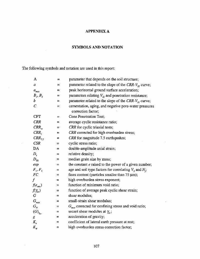
APPENDIX A
SYMBOLS AND NOTATION
The following symbols and notation are used in this report:
A =a =amax =B1,B2 =b =C =
CPT =CRR =CRRtx =CRR/ =CRR7.s =CSR =DA =Dr =Dso =exp =Fl' F2 =FC =j =j(emin) =j(tv) =G =Gmax =GN =(G)rav =g =Ko =Ku =
parameter that depends on the soil structure;
parameter related to the slope of the CRR-VS1 curve;
peak horizontal ground surface acceleration;
parameters relating VS1 and penetration resistance;
parameter related to the slope of the CRR-VS1 curve;
cementation, aging, and negative pore-water pressures
correction factor;
Cone Penetration Test;
average cyclic resistance ratio;
CRR for cyclic triaxial tests;
CRR corrected for high overburden stress;
CRR for magnitude 7.5 earthquakes;
cyclic stress ratio;
double-amplitude axial strain;
relative density;
median grain size by mass;the constant e raised to the power of a given number;age and soil type factors for correlating Vs and Nj;fines content (particles smaller than 75 ~m);
high overburden stress exponent;function of minimum void ratio;
function of average peak cyclic shear strain;
shear modulus;
small-strain shear modulus;
Gmax corrected for confining stress and void ratio;
secant shear modulus at tv;acceleration of gravity;
coefficient of lateral earth pressure at rest;high overburden stress correction factor;
107

In = natural logarithm function;MSF = magnitude scaling factor;Mw = earthquake moment magnitude;
m = stress exponent;
~ = SPT blow count in Japanese practice;
N60 = SPT energy-corrected blow count;
(N1)60 = SPT energy- and overburden stress-corrected blow count;n = magnitude scaling factor exponent;Pa = reference overburden stress (= 100 kPa);PL probability of liquefaction occurrenceTc = factor to account for effects of multidirectional shaking;Td shear stress reduction coefficient;SASW = Spectral-Analysis-of-Surface-Waves;
SePT = Seismic Cone Penetration Test;
sin = sine function;
SPT = Standard Penetration Test;
Sres = residual standard deviation;
Vs = small-strain shear wave velocity;VS1 = overburden stress-corrected Vs;
~I = limiting upper value of VS1 for liquefaction occurrence;
VS1m = mean stress-corrected Vs;
z = depth;
a(z) = function of depth;
{3(z) = function of depth;
'Yav = average peak cyclic shear strain;
p = mass density of soil;
ad = cyclic deviator stress in cyclic triaxial tests;
a' initial effective horizontal confining stress;h
a' mean effective confining stress;m
a' = initial effective confining stress in cyclic triaxial tests;0
av total vertical (or overburden) stress;a' = initial effective vertical (or overburden) stress;v
'X'av = average cyclic equivalent uniform shear stress generated byearthquake; and
'X'max = maximum cyclic shear stress generated by earthquake.
108

APPENDIXB
GLOSSARY OF TERMS
The following definitions apply to this report:
Case History
Critical Layer
Liquefaction
Occurrence
Moment Magnitude
Overburden Stress
Corrected Shear Wave
Velocity
Peak Horizontal Ground
Surface Acceleration
Shear Wave Velocity
Shear Wave
An earthquake and a test array.
The layer of non-plastic soil below the ground water table where
corrected values of shear wave velocity and penetration are the
least, and where cyclic stress ratios are the greatest.
Surface manifestations of excess pore-water pressure at depth,
such as sand boils, ground cracks and fissures, and ground
settlement.
An earthquake magnitude scale defined in terms of energy.
Shear wave velocity measurement corrected to a reference
vertical (or overburden) stress of 100 kPa.
The peak value in a horizontal ground surface acceleration
record that would occur at the site in the absence of liquefaction
or excess pore-water pressures.
The velocity of a propagating shear wave within a material witheither the direction of wave propagation or the direction ofparticle motion in the vertical direction.
A body wave with the direction of particle motion transverse to
the direction of wave propagation.
109

Test Array The two boreholes used for crosshole measurements, the boreholeand source used for downhole measurements, the cone soundingand source used for seismic cone measurements, the boreholeused for suspension logging measurements, or the line of
receivers used for Spectral-Analysis-of-Surface-Waves (SASW)
measurements.
110

APPENDIXC
SUMMARY OF CASE mSTORY DATA
Table C.1 presents a summary of case history data described in Chapter 3, and used inChapter 4 to establish the recommended liquefaction resistance curves. This database has beenexpanded and modified from the database presented by Andrus and Stokoe (1997). Most of themodifications are minor with the intent to have the data conform to the draft guidelinespresented in this document. The major modifications are based on new information orcorrection of an error in calculations. Some case histories included in the earlier database byAndrus and Stokoe have been omitted due to one of the three following reasons: (1) Thereported average downhole Vs measurement is for a depth interval much greater than theidentified critical layer. (2) The critical layer is likely older than 10 000 years and containscarbonate. (3) The location of the critical layer or field behavior is uncertain. References forthe case history data are given in Table 3.1.
111

112

.......
.......u.>
Table C.l - Summary Infonnation for Vs -Based Liquefaction and Non-Liquefaction Case Histories.
-··General Characteristics of Critical Laver···· ····Averaae Value for Critical LaVE r····Too No. of
SuI. Water of Averaae Values Elf.Test L1o. Table amax. Laver Thick Soil Fines Deoosi in Vert. Vert. a:R
Site Tvpe Mw Eff.? Deoth avo. Death ness Tvoe Content Tvoe Aoe Average Depth Stress Stress rd Vs Vsl a:R 7.51 = Y0= N m g m m % m kPa kPa m/s m/s
1906 SAN FRANCISCO, CALIFORNIA EARTHQU KE
Coyote Creek, S·Rl Xhole 7.7 1 2.4 0.36 3.5 2.5 sand &aravel <5 AF H 3 4.6 83.3 61.9 0.97 136 153 0.30 0.32Covote Creek, Rl-R2 Xhole 7.7 1 2.4 0.36 3.5 2.5 sand &aravel <5 AF H 2 4.2 75.2 58.0 0.97 154 177 0.29 0.31Covote Creek, Rl-R3 Xhole 7.7 1 2.4 0.36 3.5 2.5 sand &gravel <5 AF H 2 4.2 75.2 58.0 0.97 161 185 0.29 0.31Covote Creek, R2-R3 Xhole 7.7 1 2.4 0.36 3.5 2.5 sand & gravel <5 AF H 3 4.6 83.3 61.9 0.97 169 191 0.30 0.32Salinas River North, S·Rl Xhole 7.7 0 6.1 0.32 9.1 2.3 sandv silt ML to SM 44 A H 3 9.9 177.2 139.8 0.90 177 163 0.24 0.25Salinas River North, Rl-R2 Xhole 7.7 0 6.1 0.32 9.1 2.3 sandv silt ML to SM 44 A H 3 9.9 177.2 139.8 0.90 195 179 0.24 0.25Salinas River North, Rl-R3 Xhole 7.7 0 6.1 0.32 9.1 2.3 sandv silt ML to SM 44 A H 3 9.9 177.2 139.8 0.90 200 184 0.24 0.25Salinas River North, R2-R3 Xhole 7.7 0 6.1 0.32 9.1 2.3 sandv sill ML to SM 44 A H 3 9.9 177.2 139.8 0.90 199 183 0.24 0.25Salinas River South, S-Rl Xhole 7.7 1 6.1 0.32 6.6 5.3 sand &sillY sand SPtoSM 14 A H 2 8.0 141.2 122.6 0.93 131 124 0.22 0.24Salinas River South, R1-R2 Xhole 7.7 1 6.1 0.32 6.6 5.3 sand & sillY sand SPtoSM 14 A H 2 8.0 141.2 122.6 0.93 149 141 0.22 0.24Salinas River South. R1-R3 Xhole 7.7 1 6.1 0.32 6.6 5.3 sand &sillY sand SPto SM 14 A H 2 8.0 141.2 122.6 0.93 158 151 0.22 0.24Salinas River South, R2-R3 Xhole 7.7 1 6.1 0.32 6.6 5.3 sand & sillY sand SP to SM 14 A H 2 8.0 141.2 122.6 0.93 168 159 0.22 0.24
1957 DALY CITY, CALIFORNIA EARTHQU KE
Marina District, No.2 SASW 5.3 0 2.9 0.11 2.9 7.1 sand to siltv sand eSP-SM) -8 FH R 1 6.4 117.0 82.2 0.94 120 129 0.09 0.04Marina District, No. 3 SASW 5.3 0 2.9 0.11 2.9 7.1 sand to sillY sand (SP to SM) -12 FH R 1 6.4 117.0 82.2 0.94 105 113 0.09 0.04Marina District, No.4 SASW 5.3 0 2.9 0.11 2.9 2.1 sand rSPl <5 FH R 1 3.9 69.9 59.6 0.98 120 137 0.08 0.03Marina District, No. 5 SASW 5.3 0 5.9 0.11 5.9 4.1 sand eSPl <5 Dune? H? 1 7.9 140.6 120.5 0.93 220 211 0.08 0.03Marina District, school Dhole 5.3 0 2.7 0.11 2.7 1.6 sand (SP) 2 RJ R 2 3.5 62.3 54.1 0.98 112 130 0.08 0.03
1964 NIIGATA, JAPAN EARTHQUAKE
Niigata, Railway-Station ? 7.5 1 2.0 0.16 2.0 2.7 sand <5 ? ? 2 3.2 56.7 45.2 0.98 131 160 0.13 0.13Niiaata, Site A1 SASW 7.5 0 5.0 0.16 5.0 2.5 sand <5 ? ? 1 6.2 109.9 97.7 0.95 162 164 0.12 0.12Niiaata, Site Cl SASW 7.5 1 1.2 0.16 1.6 6.5 sand <5 ? ? 2 4.5 82.8 50.7 0.97 112 136 0.15 0.15Niigata. Site C2 SASW 7.5 1 1.2 0.16 1.2 4.8 sand <5 ? ? 1 4.0 73.4 46.5 0.97 118 147 0.15 0.15
1975 HAICHENG, PRC EARTHQUAKE
Chemical Fibre Dhole 7.3 1 1.5 0.12 6.0 5.5 sand to siltv clav 61 ? ? 3 8.6 159.7 90.3 0.92 147 151 0.13 0.12Construction Buildina Dhole 7.3 1 1.5 0.12 3.0 6.5 clavev silt to sillY clav 83 ? ? 2 6.8 124.8 73.6 0.95 103 111 0.13 0.12Fisheries &Shlobuildina Dhole 7.3 1 0.5 0.12 2.5 4.0 siltv sand to c1avev silt 90 ? ? 4 4.4 81.7 43.7 0.97 101 124 0.14 0.13Glass Fiber Dhole 7.3 1 0.8 0.12 2.7 3.8 sandv silt to c1avev silt 42 ? ? 3 4.8 89.8 50.3 0.97 98 117 0.13 0.13Middle School Dhole 7.3 0 1.0 0.12 5.0 6.0 c1avev silt to siltv clav 92 ? ? 2 10.2 191.6 100.9 0.90 143 143 0.13 0.12PaoerMili Dhole 7.3 1 1.0 0.12 2.5 2.5 clavev sill to sillv clav 72 ? ? 1 3.0 54.7 35.2 0.98 122 158 0.12 0.11
Test Type
Xhole = crosshole seismic test
Dhole =downhole seismic testSCPT =Seismic Cone Penetration Test
SASW = Spectral-Analysis·of·Surface·Waves test
Susp. =suspension logger test
Deposit Type
F = fillFH =fill, hydraulicFD = fill, dumped
FU =fill, uncompactedFI =fill, improved
A =AlluvialAF =Alluvial, fluvialVDF =volcanic debris flow
~R = Recent « 500 years)H =Holocene « 10 000 years)
CSR 7.5 = CSRI(Mv/7.5r2.56
? = unknown

........+:-
Table C.I - Summary Information for Vs -Based Liquefaction and Non-Liquefaction Case Histories.
····General Characteristics of Crillcal Laver---· ----Averaae Value for Critical LaVE r ----Top No. of
Suf. Water of Averaae Values Eft.Test L1a. Table amax. Laver Thick Soli Fines Deooslt In Vert. Vert. a:R
Site Tvoe Mw Elf.? Depth avo. Depth ness Tvpe Content Tvpe Aae Averaae Deoth Stress Stress rd Vs Vsl a:R 7.51 =yO=N m a m m % m kPa kPa m/s m/s
1979 IMPERIAL VALLEY EARTHQUAKE
Heber Road Channel Fill, Rl-R2 Xhole 6.5 1 1.8 0.50 2.0 2.7 slltv sand (SM) 22 AF R 4 3.5 63.2 46.8 0.98 131 159 0.42 0.29Heber Road Channel Fill, S-Rl Xhole 6.5 1 1.8 0.50 2.0 2.7 siltv sand (SM) 22 AF R 4 3.5 63.2 46.8 0.98 133 161 0.42 0.29Heber Road Point Bar, Rl-R2 Xhole 6.5 0 1.8 0.50 1.8 2.4 sand wlsilt (SP-SM) 10 AF R 4 3.4 60.3 45.4 0.98 164 201 0.42 0.29Heber Road Poinl Bar, S-Rl Xhole 6.5 0 1.8 0.50 1.8 2.4 sand wlsilt (SP-SM) 10 AF R 4 3.4 60.3 45.4 0.98 173 211 0.42 0.29Kornbloom SASW 6.5 0 2.4 0.12 2.5 3.5 sandv slit (MLl 75 AF R 5 4.2 75.1 58.1 0.97 105 120 0.10 0.07McKim SASW 6.5 1 1.5 0.51 1.5 3.5 slltv sand (SMl 20 AF R 4 3.0 54.1 39.7 0.98 126 160 0.43 0.30Radio Tower SASW 6.5 1 2.0 0.21 2.7 3.4 slllv sand to sandv slit (SM 10 MLl 35 AF H? 5 4.4 79.2 55.8 0.97 90 104 0.19 0.13Vall Canal SASW 6.5 0 2.7 0.12 2.7 2.8 sand wI silt to slllv sand (SP-SM to SMl 13 AF R 4 4.0 70.4 58.4 0.98 101 116 0.09 0.06Wildlife SASW 6.5 0 1.5 0.13 2.5 4.3 slllv sand to sandv sill (SM to MLl 27 AF R 5 4.7 86.7 55.3 0.97 114 133 0.13 0.09Wildlife 1 Xhole 6.5 0 1.5 0.13 2.5 4.3 sillv sand to sandv sill (SM to MLl 27 AF R 4 4.6 83.8 53.9 0.97 127 148 0.13 0.09Wildlife, 2 Xhole 6.5 0 1.5 0.13 2.5 4.3 slllv sand to sandv sill (SM to MLl 27 AF R 4 4.6 83.8 53.9 0.97 124 146 0.13 0.09
1980 MID-CHIBA, JAPAN EARTHQUAKE
Owl Island No.1, laver 1 dhole 5.9 0 1.3 0.08 4.5 3.3 slltv sand 20 FH R 1 6.1 111.4 65.3 0.96 155 173 0.08 0.04Owl Island No.1, laver 2 dhole 5.9 0 1.3 0.08 13.0 3.6 slltv sand 35 A H 1 14.8 255.8 124.5 0.77 195 185 0.08 0.04
1981 WESTMORLAND, CALIFORNIA EARTHQU KE
Heber Road Channel Fill, Rl-R2 Xhole 5.9 0 1.8 0.02 2.0 2.7 slltv sand (SMl 22 AF R 4 3.5 63.2 46.8 0.98 131 159 0.02 0.01Heber Road Channel Fill, S-Rl Xhole 5.9 0 1.8 0.02 2.0 2.7 sillv sand (SMl 22 AF R 4 3.5 63.2 46.8 0.98 133 161 0.02 0.01Heber Road Polnl Bar, Rl-R2 Xhole 5.9 0 1.8 0.02 1.8 2.4 sand wlsllt (SP-SMl 10 AF R 4 3.4 60.3 45.4 0.98 164 201 0.02 0.01Heber Road Point Bar, S-Rl Xhole 5.9 0 1.8 0.02 1.8 2.4 sand wlsllt (SP-SMl 10 AF R 4 3.4 60.3 45.4 0.98 173 211 0.02 0.01Kornbloom SASW 5.9 1 2.4 0.36 2.5 3.5 sandv silt (MLl 75 AF R 5 4.2 75.1 58.1 0.97 105 120 0.29 0.16McKim SASW 5.9 0 1.5 0.06 1.5 3.5 sillv sand (SMl 20 AF R 4 3.0 54.1 39.7 0.98 126 160 0.05 0.03Radio Tower SASW 5.9 1 2.0 0.20 2.7 3.4 sillv sand 10 sandv sill (SM to ML) 35 AF H? 5 4.4 79.2 55.8 0.97 90 104 0.18 0.10Vail Canal SASW 5.9 1 2.7 0.30 2.7 2.8 sand wI silt to sillv sand (SP-SM to SM) 13 AF R 4 4.0 70.4 58.4 0.98 101 116 0.23 0.12Wildlife SASW 5.9 1 1.5 0.27 2.5 4.3 silty sand to sandv silt (SM to ML) 27 AF R 5 4.7 86.7 55.3 0.97 114 133 0.26 0.14Wildlife, 1 Xhole 5.9 1 1.5 0.27 2.5 4.3 silty sand to sandv silt (SM to ML) 27 AF R 4 4.6 83.8 53.9 0.97 127 148 0.26 0.14Wildlife, 2 Xhole 5.9 1 1.5 0.27 2.5 4.3 silty sand to sandv silt (SM to ML) 27 AF R 4 4.6 83.8 53.9 0.97 124 146 0.26 0.14
..
Test Type
Xhole =crosshole seismic testDhole =downhole seismic test
SCPT =Seismic Cone Penetration Test
SASW = Spectral-Analysis-of-Surface-Waves testSusp. =suspension logger test
Deposit Type
F = fillFH = fill, hydraulicFD = fill, dumped
FU =fill, uncompactedFI =fill, improved
A =Alluvial
AF =Alluvial, fluvial
VDF =volcanic debris flow
~R =Recent « 500 years)
H = Holocene « 10 000 years)
CSR 7.5 =CSRI(MJ7.5)'2.56
? =unknown

..........V\
Table C.l - Summary Information for Vs -Based Liquefaction and Non-Liquefaction Case Histories.
····General Characteristics of Critical Laver·..• ···-Averaee Value for Critical LaYE r ••--Too No. of
SuI. Water of Averaee Values Elf.Test Lie. Table amax. Laver Thick Soil Fines Deoosl In Vert. Vert. CS'I
Site Tvpe Mw Elf.? Depth avg. Depth ness Type Content Tvpe Age Averaae Depth Stress Stress rd Vs Vsl CS'I 7.5l=YO=N m a m m % m kPa kPa m/s m/s
1983 BORAH PEAK,IDAHO EARTHQUAK
Andersen Bar SA-l SASW 6.9 1 0.8 0.29 0.8 2.4 sandv aravel GP-GWI <5 AF R 3 1.9 39.0 27.8 0.99 105 145 0.25 0.20Andersen Bar, Xl-X2 Xhole 6.9 1 0.8 0.29 0.8 2.4 sandv aravel GP·GWI <5 AF R 8 2.0 40.6 28.7 0.99 106 146 0.26 0.21Goddard Ranch, SA-2 SASW 6.9 1 1.2 0.30 1.2 2.0 sandv Qravel GPI <5 AF H 2 2.4 49.7 37.3 0.97 122 157 0.25 0.20Goddard Ranch, SA-4 SASW 6.9 1 1.2 0.30 1.2 2.0 sandy gravel GPI <5 AF H 2 2.4 49.8 37.4 0.97 105 136 0.25 0.20Mackav Dam, Toe SASW 6.9 0 2.3 0.23 2.3 2.7 sillY sandv aravel (GW to GMI 6 ? H 2 2.8 57.2 52.3 0.98 270 318 0.16 0.13North Gravel Bar Bar Site SASW 6.9 0 1.0 0.46 1.8 1.2 sandy Qravel -<5 A H? 2 2.4 51.0 36.0 0.99 206 266 0.41 0.33North Gravel Bar, Terrace SASW 6.9 0 3.0 0.46 3.0 1.3 sandy Qravel -<5 A H? 2 3.7 75.2 69.2 0.98 274 301 0.32 0.26Pence Ranch, SA-l SASW 6.9 1 1.7 0.36 1.8 1.9 Iaravellv sand to sandy gravel <5 AF H 4 2.8 57.3 46.2 0.98 103 125 0.28 0.23Pence Ranch, SA-2 SASW 6.9 1 1.5 0.36 1.5 2.8 Igravelly sand to sandy gravel <5 AF H 3 3.1 60.3 44.7 0.98 94 115 0.30 0.25Pence Ranch, SA-3 SASW 6.9 1 1.4 0.36 1.4 1.8 gravelly sand to sandy gravel <5 AF H 3 2.4 45.8 36.8 0.98 102 131 0.28 0.23Pence Ranch SA-4 SASW 6.9 1 1.8 0.36 1.8 2.8 aravellv sand to sandy gravel <5 AF H 2 3.1 62.1 49.4 0.98 109 131 0.28 0.23Pence Ranch, SA-5 SASW 6.9 1 1.5 0.36 1.5 1.9 aravellv sand to sandy gravel <5 AF H 2 3.0 60.5 45.6 0.98 123 151 0.29 0.24Pence Ranch, SA-A SASW 6.9 1 2.0 0.36 2.0 1.7 gravelly sand to sandy gravel <5 AF H 1 2.8 57.5 46.3 0.98 134 164 0.28 0.23Pence Ranch, SA-B SASW 6.9 1 1.5 0.36 1.5 1.7 oravelly sand to sandy gravel <5 AF H 2 2.1 38.8 32.9 0.99 128 170 0.27 0.21Pence Ranch, SA-e SASW 6.9 1 1.5 0.36 1.5 1.9 aravellv sand to sandv aravel <5 AF H 2 2.1 38.4 32.4 0.99 107 142 0.27 0.21Pence Ranch, SA-D SASW 6.9 1 1.5 0.36 1.5 1.7 aravellv sand to sandv aravel <5 AF H 2 2.1 39.4 33.8 0.99 131 173 0.26 0.21Pence Ranch, SA-E SASW 6.9 1 1.7 0.36 1.7 1.5 eravellv sand to sandv aravel <5 AF H 2 2.3 43.3 38.3 0.99 122 155 0.26 0.21Pence Ranch, X().XE Xhole 6.9 1 1.5 0.36 2.8 1.0 aravellv sand to sandv aravel <5 AF H 3 3.4 64.7 46.8 0.98 146 176 0.32 0.26
1985 CHIBA-IBAARAGI, JAPAN EARTHQUAKE
Owl Island No.1, laver 1 Dhole 6.0 0 1.3 0.05 4.5 3.3 sillY sand 20 FH R 1 6.1 111.4 65.3 0.96 155 173 0.05 0.03Owl Island No.1, laver 2 Dhole 6.0 0 1.3 0.05 13.0 3.6 sillY sand 35 A H 1 14.8 255.8 124.5 0.77 195 185 0.05 0.03
10/26/85 TAIWAN EARTHQUAKE EVENT LS T21
Loluna LSST, L2-L5/L6 Xhole 5.3 0 0.5 0.05 3.7 5.2 sil!V sand to sandv slit SM-ML 50 A H 3 6.1 114.1 45.4 0.96 137 167 0.08 0.03Lotuna LSST, L2-L7 Xhole 5.3 0 0.5 0.05 3.7 5.2 sil tv sand to sandv slit SM-ML 50 A H 3 6.1 114.1 45.4 0.96 127 155 0.08 0.03Loluna LSST, L8-L3 Xhole 5.3 0 0.5 0.05 4.1 4.8 sillY sand to sandv slit SM-ML 50 A H 3 6.1 114.1 45.4 0.96 156 191 0.08 0.03Lotune LSST, L8·L4 Xhole 5.3 0 0.5 0.05 3.0 5.9 sll tv sand to sandv slit SM-ML 50 A H 4 5.3 99.8 40.4 0.96 142 179 0.08 0.03
.---_._-- ..
Test Type
Xhole = crosshole seismic test
Ohole = downhole seismic testSCPT = Seismic Cone Penetration Test
SASW = Spectral-Analysis-of·Surface·Waves testSusp. = suspension logger test
Oepasit Type
F = fillFH '" fill, hydraulicFO = fill, dumped
FU = fill, uncompactedFI = fill, improved
A = AlluvialAF = AllUVial, fluvialVDF '" volcanic debris flow
iliI2R = Recent (< 500 years)H = Holocene « 10 000 years)
CSR 7.5 '" CSRI{Mv/7.5r2.56
? = unknown

............0\
Table C.1 - Summary Infonnation for Vs -Based Liquefaction and Non-Liquefaction Case Histories.
····General Characteristics of Critical Layer···· ····Average Value for Critical LavI r ••••Top No. of
Suf. Water of Average Values Elf.Test L1a. Table amax. Layer Thick Soli Fines Deposl In Vert. Vert. CS'l
Site Type Mw Elf.? Depth avg. Depth ness Type Content Type Aae Averaae Depth Stress Stress rd Vs Vsl CS'l 7.5l=YO=N m a m m % m kPa kPa m/s m/s
11/7/85 TAIWAN EARTHQUAKE (EVENT LSS 3)
Lotuna LSST, L2·L5/L6 Xhole 5.5 0 0.5 0.02 3.7 5.2 sillY sand to sandy slit SM·ML 50 A H 3 6.1 114.1 45.4 0.96 137 167 0.03 0.01Lotuna LSST, L2·L7 Xhole 5.5 0 0.5 0.02 3.7 5.2 sillY sand to sandy slit SM·ML 50 A H 3 6.1 114.1 45.4 0.96 127 155 0.03 0.01Lotuna LSST, L8·L3 Xhole 5.5 0 0.5 0.02 4.1 4.8 sillY sand to sandy silt SM·ML 50 A H 3 6.1 114.1 45.4 0.96 156 191 0.03 0.01Lotuna LSST, L8-L4 Xhole 5.5 0 0.5 0.02 3.0 5.9 sillY sand to sandy silt SM·ML 50 A H 4 5.3 99.8 40.4 0.96 142 179 0.03 0.01
1/16/86 TAIWAN EARTHQUAKE (EVENT LSS 4)
Lotung LSST, L2·L5/L6 Xhole 6.6 0 0.5 0.22 3.7 5.2 sillY sand to sandy sill SM·ML 50 A H 3 6.1 114.1 45.4 0.96 137 167 0.34 0.25LotunQ LSST, L2·L7 Xhole 6.6 0 0.5 0.22 3.7 5.2 sillY sand to sandY silt SM·ML 50 A H 3 6.1 114.1 45.4 0.96 127 155 0.34 0.25Lotung LSST, L8·L3 Xhole 6.6 0 0.5 0.22 4.1 4.8 sillY sand to sandy sill SM·ML 50 A H 3 6.1 114.1 45.4 0.96 156 191 0.34 0.25Lotung LSST L8·L4 Xhole 6.6 0 0.5 0.22 3.0 5.9 sillY sand to sandy slit SM·ML 50 A H 4 5.3 99.8 40.4 0.96 142 179 0.34 0.24
4/8/86 TAIWAN EARTHQUAKE (EVENT LSST 6)
Lotuna LSST, L2·L5/L6 Xhole 5.4 0 0.5 0.04 3.7 5.2 sillY sand to sandy silt {SM·ML 50 A H 3 6.1 114.1 45.4 0.96 137 167 0.06 0.03LotunQ LSST L2·L7 Xhole 5.4 0 0.5 0.04 3.7 5.2 sillY sand to sandy slit {SM-ML 50 A H 3 6.1 114.1 45.4 0.96 127 155 0.06 0.03Lotung LSST, L8·L3 Xhole 5.4 0 0.5 0.04 4.1 4.8 sillY sand to sandv slit ISM-ML 50 A H 3 6.1 114.1 45.4 0.96 156 191 0.06 0.03Lotung LSST L8-L4 Xhole 5.4 0 0.5 0.04 3.0 5.9 sillY sand to sandv slit ISM·ML 50 A H 4 5.3 99.8 40.4 0.96 142 179 0.06 0.03
5/20/86 TAIWAN EARTHQUAKE (EVENT LSS 7)
Lotung LSST, L2-L5/L6 Xhole 6.6 0 0.5 0.18 3.7 5.2 sillY sand to sandY slit SM·ML 50 A H 3 6.1 114.1 45.4 0.96 137 167 0.28 0.20Lotung LSST, L2·L7 Xhole 6.6 0 0.5 0.18 3.7 5.2 sillY sand to sandy silt SM-ML 50 A H 3 6.1 114.1 45.4 0.96 127 155 0.28 0.20LotunQ LSST, L8·L3 Xhole 6.6 0 0.5 0.18 4.1 4.8 silty sand to sandy slit SM-ML 50 A H 3 6.1 114.1 45.4 0.96 156 191 0.28 0.20Lotung LSST, L8·L4 Xhole 6.6 0 0.5 0.18 3.0 5.9 sillY sand to sandy slit SM·ML 50 A H 4 5.3 99.8 40.4 0.96 142 179 0.27 0.20
5/20/86 TAIWAN EARTHQUAKE EVENT LSSIT 8)
Lotuna LSST, L2·L5/L6 Xhole 6.2 0 0.5 0.04 3.7 5.2 sillY sand to sandy sill SM·ML 50 A H 3 6.1 114.1 45.4 0.96 137 167 0.06 0.04Lotuna LSST, L2-L7 Xhole 6.2 0 0.5 0.04 3.7 5.2 sillY sand to sandy sill SM·ML 50 A H 3 6.1 114.1 45.4 0.96 127 155 0.06 0.04Lotuna LSST, L8·L3 Xhole 6.2 0 0.5 0.04 4.1 4.8 sillY sand to sandy sill SM·ML 50 A H 3 6.1 114.1 45.4 0.96 156 191 0.06 0.04Lotuna LSST, L8-L4 Xhole 6.2 0 0.5 0.04 3.0 5.9 sillY sand to sandy slit SM·ML 50 A H 4 5.3 99.8 40.4 0.96 142 179 0.06 0.04
1---
Test Type
Xhole = crosshole seismic testDhole = downhole seismic testSCPT = Seismic Cone Penetration Test
SASW = Spectral·Analysls·of-Surface-Waves testSusp. = suspension logger test
Deposit Type
F = fillFH = fill, hydraulicFD = fill, dumped
FU = fill, uncompactedFI = fill, improved
A = AlluvialAF = Alluvial, fluvialVDF = volcanic debris flow
~R = Recent « 500 years)H = Holocene « 10 000 years)
CSR 7.5 = CSRI(Mv/7.5r2.56
? = unknown

I--'I--''-l
Table C.l - Summary Information for Vs -Based Liquefaction and Non-Liquefaction Case Histories.
--··General Characteristics of Critical Laver···· ·--·AveraCle Value for Critical LaYl r _•••Too No. of
Suf. Water of Averaae Values Elf.Test L1a. Table amax. Laver Thick Soli Fines Deoos! In Vert. Vert. CS'l
Site Type Mw Elf.? Deoth ava. Deoth ness Tvoe Content Tvoe Aae Averaae Deoth Stress Stress rd Vs Vsl CS'l 7.51 = YO=N m a m m % m kPa kPa m/s m/s
7/30/86 TAIWAN EARTHQUAKE (EVENT LSS 121
Lotuna LSST, L2-L5/L6 Xhole 6.2 0 0.5 0.18 3.7 5.2 slltv sand to sandy silt SM-ML 50 A H 3 6.1 114.1 45.4 0.96 137 167 0.28 0.17Lotuna LSST, L2-L7 Xhole 6.2 0 0.5 0.18 3.7 5.2 slltv sand to sandY slit SM-ML 50 A H 3 6.1 114.1 45.4 0.96 127 155 0.28 0.17Lotuna LSST, L8-L3 Xhole 6.2 0 0.5 0.18 4.1 4.8 slltv sand to sandY slit SM-ML 50 A H 3 6.1 114.1 45.4 0.96 156 191 0.28 0.17Lotuna LSST, L8-L4 Xhole 6.2 0 0.5 0.18 3.0 5.9 siltv sand to sandY slit SM-ML 50 A H 4 5.3 99.8 40.4 0.96 142 179 0.27 0.17
7/30/86 TAIWAN EARTHQUAKE (EVENT LSS 13\
Lotuna LSST, L2-L5/L6 Xhole 6.2 0 0.5 0.05 3.7 5.2 siltv sand to sandy silt SM-ML 50 A H 3 6.1 114.1 45.4 0.96 137 167 0.08 0.05Lotuna LSST, L2-L7 Xhole 6.2 0 0.5 0.05 3.7 5.2 slltv sand to sandy slit SM·ML 50 A H 3 6.1 114.1 45.4 0.96 127 155 0.08 0.05Lotuna LSST, L8-L3 Xhole 6.2 0 0.5 0.05 4.1 4.8 siltv sand to sandy silt SM-ML 50 A H 3 6.1 114.1 45.4 0.96 156 191 0.08 0.05Lotuna LSST, L8-L4 Xhole 6.2 0 0.5 0.05 3.0 5.9 slltv sand to sandy slit SM-ML 50 A H 4 5.3 99.8 40.4 0.96 142 179 0.08 0.05
11/14/86 TAIWAN EARTHQUAKE EVENT LSST 16
Lotuna LSST, L2·L5/L6 Xhole 7.6 0 0.5 0.16 3.7 5.2 slltv sand to sandy silt SM-ML 50 A H 3 6.1 114.1 45.4 0.96 137 167 0.25 0.26Lotuna LSST L2-L7 Xhole 7.6 0 0.5 0.16 3.7 5.2 slltv sand to sandy slit SM-ML 50 A H 3 6.1 114.1 45.4 0.96 127 155 0.25 0.26Lotuna LSST, L8-L3 Xhole 7.6 0 0.5 0.16 4.1 4.8 siltv sand to sandY slit SM-ML 50 A H 3 6.1 114.1 45.4 0.96 156 191 0.25 0.26Lotuna LSST, L8-L4 Xhole 7.6 0 0.5 0.16 3.0 5.9 slltv sand to sandy silt SM-ML 50 A H 4 5.3 99.8 40.4 0.96 142 179 0.24 0.25
1987 CHIBA-TOHO-OKI, JAPAN EARTHQUAKEI
Sunamachi, Tokvo Bay IDhole 6.5 0 6.2 0.10 6.2 5.8 sand with slit to slltv sand 15 FH R 2 9.0 166.8 138.8 0.92 150 141 0.06 0.04I
1987 ELMORE RANCH EARTHQUAKE
Heber Road Channel Fill, Rl·R2 Xhole 5.9 0 1.8 0.03 2.0 2.7 slltv sand ISM\ 22 AF R 4 3.5 63.2 46.8 0.98 131 159 0.03 0.01Heber Road Channel Fill, S-Rl Xhole 5.9 0 1.8 0.03 2.0 2.7 siltv sand ISM\ 22 AF R 4 3.5 63.2 46.8 0.98 133 161 0.03 0.01Heber Road Point Bar. Rl-R2 Xhole 5.9 0 1.8 0.03 1.8 2.4 sand wlsilt ISP·SMI 10 AF R 4 3.4 60.3 45.4 0.98 164 201 0.03 0.01Heber Road Point Bar, S-Rl Xhole 5.9 0 1.8 0.03 1.8 2.4 sand wlsilt ISP-SMI 10 AF R 4 3.4 60.3 45.4 0.98 173 211 0.03 0.01Kornbloom SASW 5.9 0 2.4 0.24 2.5 3.5 sandy silt IMLl 75 AF R 5 4.2 75.1 58.1 0.97 105 120 0.19 0.10McKim SASW 5.9 0 1.5 0.06 1.5 3.5 siltv sand ISM\ 20 AF R 4 3.0 54.1 39.7 0.98 126 160 0.05 0.03Radio Tower SASW 5.9 0 2.0 0.11 2.7 3.4 silty sand to sandy slit (SM to ML) 35 AF H? 5 4.4 79.2 55.8 0.97 90 104 0.10 0.05Vail Canal SASW 5.9 0 2.7 0.13 2.7 2.8 sand wI silt to silty sand (SP-SM to SM) 13 AF R 4 4.0 70.4 58.4 0.98 101 116 0.10 0.05Wildlife SASW 5.9 0 1.5 0.13 2.5 4.3 silty sand to sandy silt (SM to ML) 27 AF R 5 4.7 86.7 55.3 0.97 114 133 0.13 0.07Wildlife, 1 Xhole 5.9 0 1.5 0.13 2.5 4.3 silty sand to sandy silt (SM to MLl 27 AF R 4 4.6 83.8 53.9 0.97 127 148 0.13 0.07Wildlife 2 Xhole 5.9 0 1.5 0.13 2.5 4.3 sillv sand to sandy silt (SM to MLl 27 AF R 4 4.6 83.8 53.9 0.97 124 146 0.13 0.07
Test Type
Xhole = crosshole seismic testDhole = downhole seismic testSCPT = Seismic Cone Penetration Test
SASW = Spectral-Analysis-of·Surface-Waves testSusp. = suspension logger test
Deposit Type
F = fillFH = fill, hydraulicFD = fill, dumped
FU = fill, uncompactedFI = fill, improved
A= AlluvialAF = Alluvial, fluvialVDF = volcanic debris flow
~R = Recent « 500 years)H = Holocene « 10 000 years)
CSR 7.5 = CSRI(MJ7.5r2.56
? = unknown

......
......00
Table C.l - Summary Infonnation for Vs -Based Liquefaction and Non-Liquefaction Case Histories.
--·-General Characteristics of Critical Laver···· ····Averaae Value for Critical LavE r -_.-Too No. of
Suf. Water of Average Values Elf.Test L1Q. Table amax. Laver Thick Soli Fines DeDas! In Vert. Vert. aft
Site Tvpe Mw Elf.? Depth avg. Depth ness Type Content Type Age Average Depth Stress Stress rd Vs Vs1 aft 7.51 = Y0= N m a m m % m kPa kPa mls mls
1987 SUPERSTITION HILLS, CALIFORNIA EARTHQUA~ E
Heber Road Channel Fill, R1-R2 Xhole 6.5 0 1.8 0.18 2.0 2.7 siltv sand (SM) 22 AF R 4 3.5 63.2 46.8 0.98 131 159 0.15 0.11Heber Road Channel Fill, S-R1 Xhole 6.5 0 1.8 0.18 2.0 2.7 slltv sand (SM) 22 AF R 4 3.5 63.2 46.8 0.98 133 161 0.15 0.11Heber Road Point Bar, R1-R2 Xhole 6.5 0 1.8 0.18 1.8 2.4 sand wlsilt (Sp·SM) 10 AF R 4 3.4 60.3 45.4 0.98 164 201 0.15 0.10Heber Road Point Bar, S-R1 Xhole 6.5 0 1.8 0.18 1.8 2.4 sand wlsllt (SP-SM) 10 AF R 4 3.4 60.3 45.4 0.98 173 211 0.15 0.10Kornbloom SASW 6.5 0 2.4 0.21 2.5 3.5 sandv slit (MU 75 AF R 5 4.2 75.1 58.1 0.97 105 120 0.17 0.12McKim SASW 6.5 0 1.5 0.19 1.5 3.5 silty sand (SM) 20 AF R 4 3.0 54.1 39.7 0.98 126 160 0.16 0.11Radio Tower SASW 6.5 0 2.0 0.20 2.7 3.4 silty sand to sandy slit (SM to ML) 35 AF H? 5 4.4 79.2 55.8 0.97 90 104 0.18 0.12Vail Canal SASW 6.5 0 2.7 0.20 2.7 2.8 sand wI silt to silty sand (SP-SM to SM) 13 AF R 4 4.0 70.4 58.4 0.98 101 116 0.15 0.10Wildlife SASW 6.5 1 1.5 0.20 2.5 4.3 silty sand to sandy silt (SM to ML) 27 AF R 5 4.7 86.7 55.3 0.97 114 133 0.20 0.14Wildlife, 1 Xhole 6.5 1 1.5 0.20 2.5 4.3 silty sand to sandy slit (SM to ML) 27 AF R 4 4.6 83.8 53.9 0.97 127 148 0.19 0.13Wildlife, 2 Xhole 6.5 1 1.5 0.20 2.5 4.3 silty sand to sandy silt (SM to ML) 27 AF R 4 4.6 83.8 53.9 0.97 124 146 0.19 0.13
1989 LOMA PRIETA, CALIFORNIA EARTHQUAK i=
Bav Farm Island Dike SASW 7.0 0 3.6 0.27 3.6 2.8 sand with fines (SP-SM) 10 R R 1 5.2 91.9 77.0 0.96 204 219 0.20 0.16Bav Farm Island, Dike S·R1 Xhole 7.0 0 3.6 0.27 3.6 2.8 sand with fines (SP-SM) 10 R R 5 4.9 87.1 75.2 0.97 193 207 0.20 0.16Bav Farm Island, Dike R1-R2 Xhole 7.0 0 3.6 0.27 3.6 2.8 sand with fines (SP-SM) 10 R R 4 4.9 81.4 72.4 0.97 205 222 0.19 0.16Bav Farm Island, Loop SASW 7.0 1 3.5 0.27 3.5 1.7 sand with fines <12 FH R 1 3.8 66.7 61.4 0.98 125 142 0.18 0.15Bav Farm Island, Loop S-R1 Xhole 7.0 1 3.5 0.27 3.5 1.7 sand with fines <12 FH R 3 4.3 75.6 68.2 0.98 98 107 0.19 0.16Bav Farm Island LOaD R1-R2 Xhole 7.0 1 3.5 0.27 3.5 1.7 sand with fines <12 FH R 3 4.3 75.6 68.2 0.98 113 124 0.19 0.16Covote Creek, S-R1 Xhole 7.0 0 2.4 0.18 3.5 2.5 sand & gravel <5 AF H 3 4.6 83.3 61.9 0.97 136 153 0.15 0.13Covote Creek, R1-R2 Xhole 7.0 0 2.4 0.18 3.5 2.5 sand & gravel <5 AF H 2 4.2 75.2 58.0 0.97 154 177 0.15 0.12Covote Creek, R1·R3 Xhole 7.0 0 2.4 0.18 3.5 2.5 sand & gravel <5 AF H 2 4.2 75.2 58.0 0.97 161 185 0.15 0.12Covote Creek, R2-R3 Xhole 7.0 0 2.4 0.18 3.5 2.5 sand & gravel <5 AF H 3 4.6 83.3 61.9 0.97 169 191 0.15 0.13Harbor Office, UC-12 OCPT 7.0 1 1.9 0.25 3.0 1.6 silty sand 15 ? H 2 4.1 74.3 52.6 0.97 150 176 0.22 0.19Marina District, No.2 SASW 7.0 1 2.9 0.15 2.9 7.1 sand to silty sand (SP-SM) -8 FH R 1 6.4 117.0 82.2 0.94 120 129 0.12 0.10Marina District, No. 3 SASW 7.0 1 2.9 0.15 2.9 7.1 sand to silty sand (SP to SM) -12 R-I R 1 6.4 117.0 82.2 0.94 105 113 0.12 0.10Marina District, No.4 SASW 7.0 1 2.9 0.15 2.9 2.1 sand SP <5 R-I R 1 3.9 69.9 59.6 0.98 120 137 0.11 0.09Marina District, No.5 SASW 7.0 0 5.9 0.15 5.9 4.1 sand SP <5 Dune? H? 1 7.9 140.6 120.5 0.93 220 211 0.10 0.09Marina District school Ohole 7.0 1 2.7 0.15 2.7 1.6 sand SP 2 RJ R 2 3.5 62.3 54.1 0.98 112 130 0.11 0.09Port of Oakland, POO7-1 OCPT 7.0 1 3.0 0.24 5.0 4.0 sand SP <5 R-I R 3 7.2 131.5 90.4 0.94 148 152 0.21 0.18Port of Oakland, POO7-2 SASW 7.0 1 3.0 0.24 5.0 4.0 sand SP <5 FH R 2 6.4 115.7 82.9 0.95 157 165 0.21 0.17Port of Oakland, POO7·2 OCPT 7.0 1 3.0 0.24 5.0 4.0 sand SP <5 R-I R 3 7.2 131.8 90.7 0.94 151 155 0.21 0.18Port of Oakland, P007-2, S-R1 Xhole 7.0 1 3.0 0.24 5.0 4.0 sand SP) <5 R-I R 6 7.0 127.4 88.5 0.95 147 152 0.21 0._1.!!Port of Oakland P007-2 R1-R2 Xhole 7.0 1 3.0 0.24 5.0 4.0 sand SPI <5 FH R 6 7.0 127.4 88.5 0.95 181 186 0.21 0.18
Test Type
Xhole = crosshole seismic testDhole = downhole seismic testSCPT = Seismic Cone Penetration Test
SASW = Spectral-Analysis-of-Surface-Waves testSusp. = suspension logger test
Deposit Type
F = fillFH = fill, hydraulicFD = fill, dumped
FU = fill, uncompactedFI = fill. Improved
A= AlluvialAF = Alluvial. fiuvialVDF = volcanic debris flow
892R = Recent « 500 years)H = Holocene « 10 000 years)
CSR 7.5 = CSRI(Mv/7.5r2.56
? = unknown

I-"I-"
\0
Table C.l - Summary Infonnation for Vs -Based Liquefaction and Non-Liquefaction Case Histories.
·---General Characteristics 01 Critical Laver---· -·--Averaae Value lor Critical Lavl r ••••Top No. of
Suf. Water of Averaae Values Eft.Test Lia. Table amax. Laver Thick Soli Fines Deposit In Vert. Vert. cs:l
Site Tvpe Mw Eft.? Depth avo. Depth ness Tvpe Content Tvpe Aae Averaae Depth Stress Stress rd Vs Vsl cs:l 7.51 = YO=N m g m m % m kPa kPa mls mls
Port of Oakland, POO7-3 SCPT 7.0 1 3.0 0.24 5.5 1.5 sand with silt ISP·SM) 10 FH R 1 6.2 112.7 81.3 0.95 176 185 0.21 0.17Port of Richmond, POR·2 SCPT 7.0 1 3.5 0.16 4.0 4.0 slit IMU 57 FH R 4 5.8 102.9 80.9 0.96 145 152 0.13 0.10Port of Richmond POR-2 SASW 7.0 1 3.5 0.16 4.0 4.0 silt /MU 57 FH R 2 5.3 93.6 76.4 0.97 117 125 0.12 0.10Port of Richmond, POR-2, S-Rl Xhole 7.0 1 3.5 0.16 4.0 4.0 slit /MU 57 FH R 7 6.1 109.4 84.1 0.95 143 150 0.13 0.11Port of Richmond, POR·2, Rl-R2 Xhole 7.0 1 3.5 0.16 4.0 4.0 silt (ML) 57 FH R 7 6.1 109.4 84.0 0.95 135 141 0.13 0.11Port of Richmond, POR-3 SCPT 7.0 1 3.5 0.16 4.0 3.0 silt to siltv sand (ML to SM) >25 FH R 3 5.2 93.4 76.3 0.96 110 118 0.13 0.11Port of Richmond, POR·4 SCPT 7.0 1 3.5 0.16 3.8 3.2 slltv sand ML to SM >32 FH R 3 5.2 93.4 76.3 0.96 128 137 0.12 0.10Salinas River North S·Rl Xhole 7.0 0 6.1 0.15 9.1 2.3 sandv silt ML to SM 44 A H 3 9.9 177.2 139.8 0.90 177 163 0.11 0.09Salinas River North, Rl-R2 Xhole 7.0 0 6.1 0.15 9.1 2.3 sandv silt ML to SM 44 A H 3 9.9 177.2 139.8 0.90 195 179 0.11 0.09Salinas River North, Rl-R3 Xhole 7.0 0 6.1 0.15 9.1 2.3 sandv silt ML to SM 44 A H 3 9.9 177.2 139.8 0.90 200 184 0.11 0.09Salinas River North, R2·R3 Xhole 7.0 0 6.1 0.15 9.1 2.3 sandv slit ML to SM 44 A H 3 9.9 177.2 139.8 0.90 199 183 0.11 0.09Salinas River South, S-Rl Xhole 7.0 0 6.1 0.15 6.6 5.3 sand & sil y sand SPtoSM 14 A H 2 8.0 141.2 122.6 0.93 131 124 0.10 0.09Salinas River South, Rl-R2 Xhole 7.0 0 6.1 0.15 6.6 5.3 sand & sillY sand SP to SM 14 A H 2 8.0 141.2 122.6 0.93 149 141 0.10 0.09Salinas River South. Rl-R3 Xhole 7.0 0 6.1 0.15 6.6 5.3 sand & sillY sand SP to SM 14 A H 2 8.0 141.2 122.6 0.93 158 151 0.10 0.09Salinas River South. R2·R3 Xhole 7.0 0 6.1 0.15 6.6 5.3 sand &sillY sand SP to SM 14 A H 2 8.0 141.2 122.6 0.93 168 159 0.10 0.09Sandholdt Road, UC·4 Laver 1 SCPT 7.0 1 1.8 0.25 2.1 0.6 sand 2 ? H 1 2.5 44.3 37.4 0.99 91 116 0.19 0.16Sandholdt Road, UC-4 Laver 2 SCPT 7.0 0 1.8 0.25 5.9 4.1 sand 4 ? H 4 8.0 148.0 87.2 0.94 209 216 0.26 0.22Sandholdt Road UC·6 SCPT 7.0 0 1.7 0.25 3.0 4.3 sand 1 ? H 5 4.7 85.5 56.4 0.97 171 199 0.24 0.20Santa Cruz. SC02 SCPT 7.0 1 0.6 0.42 1.3 3.2 sillY sand -35? A H 11 2.9 53.6 31.2 0.98 122 164 0.45 0.38Santa Cruz. SC03 SCPT 7.0 1 2.1 0.42 2.1 2.4 sand to silty sand -12? A H 8 3.4 59.8 47.9 0.98 145 175 0.33 0.28Santa Cruz. SC04 SCPT 7.0 0 1.8 0.42 1.8 2.1 slltv sand -35? A H 7 2.9 51.7 41.3 0.98 163 202 0.33 0.28Santa Cruz, SC05 SCPT 7.0 0 2.8 0.42 3.0 1.8 slltv sand to sandv silt >35? A H 6 4.0 70.2 58.9 0.98 149 170 0.32 0.26Santa Cruz, SC13 SCPT 7.0 0 1.8 0.42 2.0 1.3 sillY sand -35? A H 4 2.8 48.9 39.9 0.98 119 149 0.33 0.27Santa Cruz, SC14 SCPT 7.0 1 1.2 0.42 1.5 1.5 sand <5? A H 5 2.3 41.2 30.7 0.99 126 169 0.36 0.30State Beach. UC-15 SCPT 7.0 1 1.8 0.25 1.8 2.8 sand 1 ? -- H 3 3.5 62.0 45.4 0.98 116 142 0.21 0.18State Beach. UC-16 SCPT 7.0 1 2.3 0.25 2.3 7.1 sand 1 ? H 7 5.5 99.8 68.2 0.96 162 179 0.22 0.18TI Fire Station, Redpath Dhole 7.0 0 1.4 0.13 4.5 2.5 siltv sand/SM) 24 FH R 1 6.9 127.1 73.3 0.95 129 142 0.14 0.11TI Fire Station Gibbs et al. Dhole 7.0 0 1.4 0.13 4.5 2.5 slltv sand/SM) 24 FH R 1 5.8 107.0 63.7 0.96 133 150 0.14 0.11TI Fire Station, 1992 SASW 7.0 0 1.4 0.13 4.5 2.5 siltv sand SM) 24 FH R 1 5.3 98.4 59.6 0.96 131 149 0.14 0.11TI Fire Station SCPT 7.0 0 1.4 0.13 4.5 2.5 siltv sand SM) 24 FH R 1 5.3 98.4 59.6 0.96 133 152 0.13 0.11TI Fire Station, 81-84 Xhole 7.0 0 1.4 0.13 4.5 2.5 sillY sand SM 24 FH R 3 5.5 101.3 60.9 0.96 137 155 0.14 0.11TI Fire Station, 82-B3 Xhole 7.0 0 1.4 0.13 4.5 2.5 sillY sand SM 24 FH R 8 5.5 101.3 60.9 0.96 129 146 0.14 0.11TI Fire Station, 82-84 Xhole 7.0 0 1.4 0.13 4.5 2.5 sillY sand SM 24 FH R 3 5.5 101.3 60.9 0.96 132 149 0.14 0.11TI Fire Station, B4-85 Xhole 7.0 0 1.4 0.13 4.5 2.5 sillY sand SM 24 FH R 3 5.5 101.3 60.9 0.96 131 148 0.14 0.11TI Fire Station, Portable Xhole 7.0 0 1.4 0.13 4.5 2.5 slltv sand SM 24 FH R 7 5.8 97.0 63.5 0.96 130 145 0.14 0.11JI Perimeter, UM03 SCPT 7.0 0 1.5 0.14 6.5 5.2 sand to clayev silty sand 13 FH R 17 9.1 174.7 99.8 0.92 173 173 0.15 0.12TI Perimeter, UM05 SCPT 7.0 1 2.4 0.14 3.3 2.3 sand to silty sand 5 FH R 8 4.6 83.7 62.5 0.97 151 169 0.12 0.10TI Perimeter UM06 SCPT 7.0 1 1.4 0.14 2.0 1.7 sand to siltv sand 5 FH R 5 2.9 53.4 38.7 0.98 123 157 0.12 0.10
Test Type
Xhole =crosshole seismic testDhole = downhole seismic testSCPT = Seismic Cone Penetration Test
SASW = Spectral-Analysis·ol-Surlace·Waves testSusp. =suspension logger test
Deposit Type
F =fillFH =fill, hydraulicFD =lill, dumped
FU =fill, uncompactedFI =fill, improved
A =AlluvialAF =Alluvial, fluvialVDF =volcanic debris Ilow
~R = Recent « 500 years)H = Holocene « 10 000 years)
CSR 7.5 = CSRI(Mv/7.5r2•56
? = unknown

l--'No
Table C.l - Summary Information for Vs -Based Liquefaction and Non-Liquefaction Case Histories.
····General Characteristics of Critical Laver···· ····Averaae Value for Critical LaVI r ••••Too No. of
Suf. Water of Averaae Values Elf.Test L1a. Table amax. Laver Thick Soli Fines Deoosl In Vert. Vert. arl
Site Tvpe Mw Elf.? Depth avg. Depth ness Type Content Type Age Average Depth Stress Stress rd Vs Vsl CS'l 7.51- YO=N m g m m % m kPa kPa m/s m/s
TI Perimeter, UM09 OCPT 7.0 1 2.7 0.14 2.7 3.8 sand to slltv sand 14 FH R 12 4.6 83.1 64.8 0.97 143 160 0.11 0.09TI Approach to Pier, SA·5b SASW 7.0 0 2.0 0.14 2.0 10.8 sand to sand with slit (SP to Sp·SM) 5 R R 3 6.6 123.7 78.1 0.94 189 206 0.13 0.11TI Aooroach to Pier, SA·6 SASW 7.0 0 2.0 0.14 2.0 10.8 sand to sand with slit (SP to Sp·SM) 5 A R 5 5.8 104.0 67.1 0.95 187 211 0.13 0.11TI Aooroach to Pier, SA·7 SASW 7.0 0 2.0 0.14 2.0 10.8 sand to sand wilh slit (SP to SP-SM) 5 A R 3 6.6 123.7 78.1 0.98 187 203 0.13 0.11Bav Bridae Toll Plaza, S·Rl Xhole 7.0 1 3.0 0.24 5.0 2.5 sand to sll tv sand SP·SM -9 RJ R 4 6.4 116.0 82.5 0.95 143 150 0.21 0.17Bav Bridae Toll Plaza, Rl·R2 Xhole 7.0 1 3.0 0.24 5.0 2.5 sand to sll tv sand SP-SM -9 RJ R 4 6.4 116.0 82.5 0.95 144 151 0.21 0.17Bav Brldae Toll Plaza, SFOBB·l OCPT 7.0 1 3.0 0.24 5.0 2.5 sand to sll tv sand Sp·SM -9 RJ R 2 6.5 117.8 83.4 0.95 148 155 0.21 0.18Bav Bridae Toll Plaza, SFOBB·2 OCPT 7.0 1 3.0 0.24 6.0 3.0 sand to sll tv sand SP·SM -13 RJ R 4 7.5 98.9 92.4 0.94 148 151 0.22 0.18
1993 KUSHIRO·OKI, JAPAN EARTHQUAK
Kushiro Port, No.2 Suso. 8.3 1 0.9 0.41 2.7 3.0 sand wilh sill (Sp·SM) 7 A H 3 4.2 74.8 41.9 0.97 152 189 0.46 0.60Kushiro Port, No. D Suso. 8.3 1 1.9 0.41 1.9 6.8 sand 5 RJ R 2 4.5 82.3 56.6 0.97 135 161 0.35 0·4£
1993 HOKKAIDO·NANSEI·OKI, JAPAN EARTHQUAKE
Pension House, BH·l Dhole 8.3 1 1.0 0.19 1.0 2.5 sandY aravel <5 VDF H 2 2.0 40.4 30.4 0.99 74 99 0.16 0.20Hakodate Port No. 1 SusP. 8.3 1 1.2 0.15 2.7 7.0 siltv sand to sand with slit (SM to SP·SM) 20 ? ? 7 7.0 112.5 55.7 0.94 131 154 0.18 0.23Hakodate Port No.2 Suso. 8.3 0 1.4 0.15 2.1 8.2 sand with slit (Sp·SM) 8 ? ? 8 6.5 107.7 57.8 0.95 143 166 0.17 0.22Hakodate Port, No.3 Suso. 8.3 1 1.4 0.15 1.5 11.5 silly sand (SM) 54 ? ? 11 7.0 117.1 62.2 0.93 124 141 0.16 0.21
1994 NORTHRIDGE, CALIFORNIA EARTHQUAK
I----Rorv Lane, M·20 OCPT 6.7 1 3.4 0.51 3.4 4.9 silty sand -10 A ? 3 5.6 100.6 78.4 0.97 160 170 0.40 0.30Rorv Lane, M-32 OCPT 6.7 1 3.4 0.51 3.4 3.3 slltv sand -10 A ? 2 5.4 97.0 76.7 0.96 152 161 0.40 0.30.BQry Lane, M-33 OCPT 6.7 1 3.4 0.51 3.4 2.1 silly sand -10 A ? 1 4.4 78.6 67.9 0.97 129 142 0.37 0.28
1995 HYOGOKEN·NANBU, JAPAN EARTHQUA~ E
·1-f--------Hanshin Exoresswav 5, 3 Suso. 6.9 1 2.1 0.50 2.1 3.2 aravellv silly sand (SP·SM to SM) 18 FD R 1 5.6 96.6 62.8 0.96 160 180 0.48 0.39Hanshln Exoresswav 5, 10 SUSD. 6.9 1 1.8 0.58 3.5 3.5 silty sandy gravel (SM) 16 FD R 4 5.5 100.8 64.6 0.96 112 126 0.56 0.45Hanshln Exoresswav 5, 14 Suso. 6.9 1 4.3 0.63 4.5 4.1 silty sandy gravel -12 FD R 4 6.5 115.7 94.2 0.95 175 178 0.48 0.38Hanshln Exoresswav 5 25 Suso. 6.9 1 3.2 0.65 5.3 6.3 aravellv sltlv sand to oravellv sand 9 FD R 5 8.8 151.6 96.7 0.92 172 173 0.60 0.48Hanshln Expressway 5, 29 Suso. 6.9 1 2.5 0.65 3.0 8.3 slltv sand to sandy aravel with slit 12 ? ? 3 7.2 123.1 77.8 0.94 167 179 0.60 0.48KNK Dhole 6.9 0 2.0 0.12 2.0 15.0 slit, sand, aravel -10 ? H 2 6.6 128.5 83.4 0.94 139 147 0.10 0.08Kobe-Nlshlnomlya EWY, 3 Suso. 6.9 0 3.7 0.63 4.4 6.1 oravellv sand·sandv aravel with sill 7 ? ? 6 7.0 126.1 93.8 0.95 175 178 0.51 0.41Kobe·Nlshlnomi~a'f:WY, 17 Suso. 6.9 0 2.0 0.53 2.0 2.5 aravellv sand with slit 8 ? ? 1 3.3 60.9 49.0 0.98 200 239 0.42 0.34Kobe·Nishlnomiva EWY 23 SUSD. 6.9 0 2.9 0.63 2.9 3.1 aravellv sand·sandv aravel with slit 11 ? ? 1 4.0 71.5 60.8 0.98 130 147 0.47 0.38
Test Type
Xhole = crosshole seismic testDhole =downhole seismic testSCPT =Seismic Cone Penetration Test
SASW = Spectral·Analysls·of·Surface·Waves testSusp. =suspension logger test
DepOSit Type
F = fillFH = fill, hydraulicFD =fill, dumped
FU =fill, uncompactedFI = fill, Improved
A = AlluvialAF = Alluvial, fluvialVDF =volcanic debris flow
892R = Recent « 500 years)H =Holocene « 10 000 years)
CSR 7.5 =CSRI(Mwl7.5r2.56
? =unknown
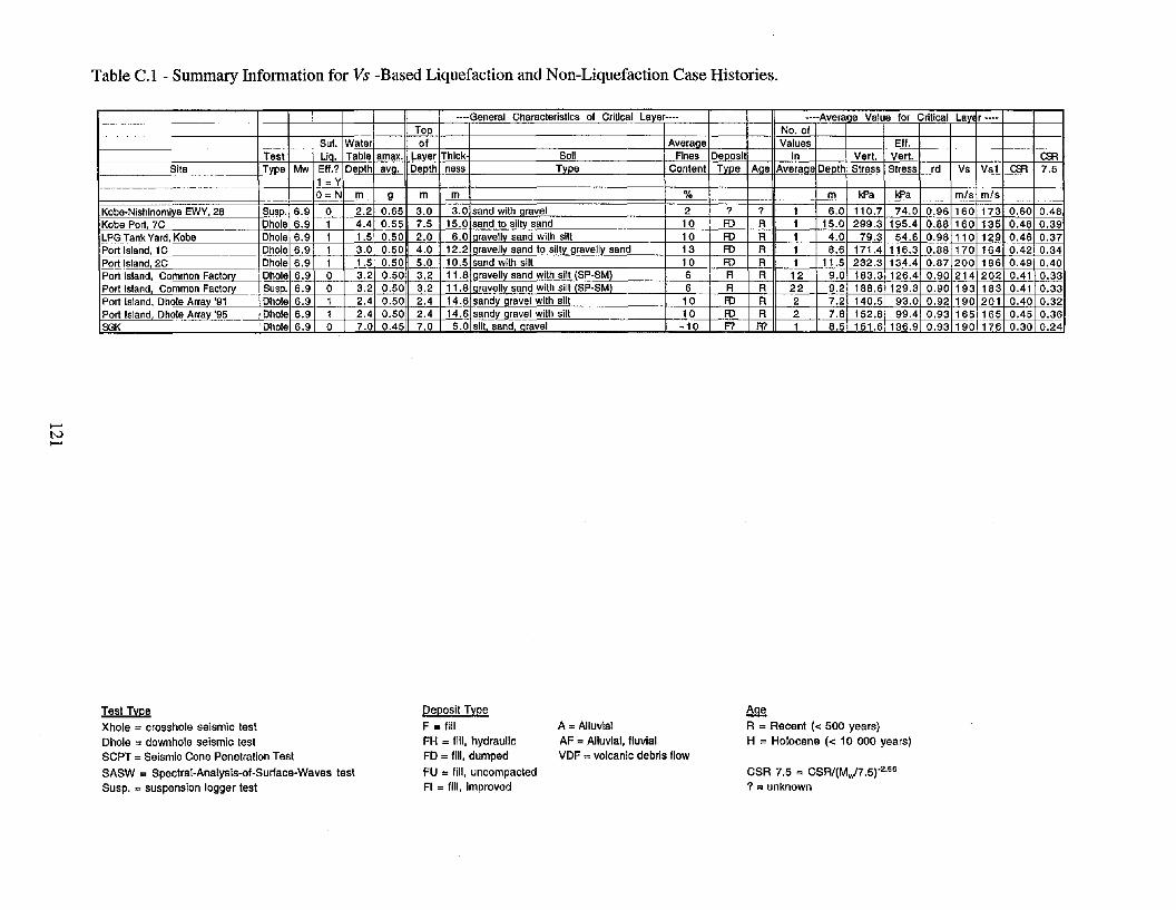
.....tv.....
Table C.I - Summary Information for Vs -Based Liquefaction and Non-Liquefaction Case Histories.
····General Characteristics of Critical Laver···· ····Averaae Value for Critical LavE r ••••Too No. of
SuI. Water of Averaae Values Elf.Test Lia. Table amax. Laver Thick Soil Fines Deoosl In Vert. Vert. a:R
Site Tvpe Mw Elf.? Deoth avo. Deoth ness Tvoe Content Tvoe Aae Averaae Deoth Stress Stress rd Vs Vsl a:R 7.51 = Y0= N m g m m % m kPa kPa mls mls
Kobe·Nishlnomlva EWY, 28 Suso. 6.9 0 2.2 0.65 3.0 3.0 sand with aravel 2 ? ? 1 6.0 110.7 74.0 0.96 160 173 0.60 0.48Kobe Port, 7C Dhole 6.9 1 4.4 0.55 7.5 15.0 sand to slltv sand 10 FD R 1 15.0 299.3 195.4 0.88 160 135 0.48 0.39LPG Tank Yard, Kobe Dhole 6.9 1 1.5 0.50 2.0 6.0 Iaravellv sand with slit 10 FD R 1 4.0 79.3 54.6 0.98 110 129 0.46 0.37Port Island, 1C Dhole 6.9 1 3.0 0.50 4.0 12.2 Iaravellv sand to sillY aravellv sand 13 FD R 1 8.6 171.4 116.3 0.88 170 164 0.42 0.34Port Island, 2C Dhole 6.9 1 1.5 0.50 5.0 10.5 sand with slit 10 FD R 1 11.5 232.3 134.4 0.87 200 186 0.49 0.40Port Island, Common Factorv Dhole 6.9 0 3.2 0.50 3.2 11.8 aravellv sand with silt eSp·SM) 6 R R 12 9.0 183.3 126.4 0.90 214 202 0.41 0.33Port Island, Common Factorv Susp. 6.9 0 3.2 0.50 3.2 11.8 aravellv sand with silt eSp·SMl 6 R R 22 9.2 188.6 129.3 0.90 193 183 0.41 0.33Port Island, Dhore Array '91 Dhole 6.9 1 2.4 0.50 2.4 14.6 sandY aravel with silt 10 FD R 2 7.2 140.5 93.0 0.92 190 201 0.40 0.32Port Island, Dhore Arrav '95 Dhole 6.9 1 2.4 0.50 2.4 14.6 sandY aravel with silt 10 FD R 2 7.8 152.8 99.4 0.93 165 165 0.45 0.36SGK Dhole 6.9 0 7.0 0.45 7.0 5.0 silt sand, aravel -10 F? R? 1 8.5 151.6 136.9 0.93 190 176 0.30 0.24
Test Type
Xhole =crosshole seismic testDhole =downhole seismic testSCPT =Seismic Cone Penetration Test
SASW =Spectral·Analysis-of-Surface-Waves testSusp. =suspension logger test
Deposit Type
F = fillFH = fill, hydraulicFD =fill, dumped
FU =fill, uncompactedFI =fill, improved
A = AlluvialAF =Alluvial, fluvialVDF = volcanic debris flow
892R = Recent « 500 years)H = Holocene « 10 000 years)
CSR 7.5 = CSRI(Mv/7.5r2 .56
? = unknown