DRAFT: EVOLUTIONARY CLUSTERING VIA MESSAGE PASSING 1

Evolutionary Clustering via Message PassingNatalia M. Arzeno and Haris Vikalo, Senior Member, IEEE

Abstract—When data are acquired at multiple points in time, evolutionary clustering can provide insights into cluster evolution andchanges in cluster memberships while enabling performance superior to that obtained by independently clustering data collected atdifferent time points. Existing evolutionary clustering methods typically require additional steps before and after the clustering stage toapproximate the number of clusters or match them across time. In this paper we introduce evolutionary affinity propagation (EAP), anevolutionary clustering algorithm that groups points by passing messages on a factor graph. The EAP algorithm promotes temporalsmoothness via factor nodes that link variable nodes across time, and introduces consensus nodes that enable cluster tracking andidentification of cluster births and deaths. Akin to the conventional (static) affinity propagation, the EAP framework automaticallydetects the number of clusters. The effectiveness of EAP is demonstrated on several simulated and real world datasets.

Index Terms—evolutionary clustering, affinity propagation, temporal data.

F

1 INTRODUCTION

E VOLUTIONARY clustering seeks to cluster data collectedat multiple points in time while taking into account

underlying dynamics and conserving temporal smoothness.The results of such an approach are typically more in-formative and generally outperform clustering conductedindependently at each time point [1], [2], [3]. In recent years,traditional clustering algorithms such as k-means, spectralclustering, and agglomerative clustering have been adaptedto the evolutionary clustering setting [1], [4], [5] and usedin a range of different applications including prediction oflinks between blogs, clustering tags from Flickr photos, andidentifying communities of spammers [1], [4], [6]. Theseevolutionary clustering algorithms modify the objective ofthe traditional clustering problems to include a term mea-suring the quality of the results at each time step as wellas a temporal smoothness term that compares the currentclustering with that performed at previous time steps andpromotes sustained cluster membership.

A limiting factor in most evolutionary as well as tra-ditional clustering methods is the necessity to provide thenumber of clusters, which is often determined using var-ious heuristics. Evolutionary clustering methods that au-tomatically decide the number of clusters typically do soby clustering with Dirichlet processes [2], [7], [8]. Ideally,evolutionary clustering algorithms should allow for varyingnumbers of clusters, i.e., they should permit that the clustersare born, evolve, or die at each time step. Additionally,algorithms should be able to handle data points that areonly present only for a subset of the time steps (i.e., datapoints can appear or be removed with time). While thereexist algorithms that can satisfy some [3], [5] or most ofthese requirements [2], [9], doing so in a practically feasiblemanner remains a challenge.

In this paper we propose evolutionary affinity propaga-

• N.M. Arzeno and H. Vikalo are with the Department of Electrical andComputer Engineering, The University of Texas at Austin, Austin, TX,78717.E-mail: narzeno@utexas.edu, hvikalo@ece.utexas.edu

tion (EAP), an evolutionary clustering algorithm that buildsupon ideas of static affinity propagation to cluster dataacquired at multiple time points by passing messages on anappropriately defined factor graph. The key distinguishingfeatures of EAP are:

1) EAP automatically determines the number of clus-ters at each time step.

2) By relying on certain consensus nodes introducedin the factor graph, EAP accurately and efficientlytracks clusters across time.

3) EAP identifies the global clustering solution bypassing messages between the nodes representingdata at different time steps.

4) The EAP output provides the cluster membershipfor each data point at each time instance.

5) The EAP framework allows having different num-bers of clusters at different time steps as well as datapoint insertions and deletions.

The EAP’s ability to automatically detect the number ofclusters is inherited from affinity propagation (AP). Similarto AP, EAP can handle non-metric similarities, and canbe efficiently implemented for large, sparse datasets. Ina departure from AP, the EAP’s cluster tracking propertyimplies that the points changing cluster membership can beidentified, along with cluster births, evolutions, and deaths.Moreover, EAP’s ability to find the global clustering solutionprevents propagation of errors that occurs in many evolu-tionary clustering methods where the clustering solution attime t is only dependent on the data or clustering solutionat t − 1 while it disregards those at t + 1 and other times.EAP provides an exemplar for each data point at each timeinstance and hence cluster memberships, both for a singletime instance as well as their evolution across time, arestraightforward to identify. Note that EAP is a data-centricclustering approach wherein points are tracked across time,contrary to distribution-based clustering methods focusingexclusively on the distributions and the evolution of theirparameters (and hence typically require an additional clus-ter assignment step). To our knowledge, EAP is the first

DRAFT: EVOLUTIONARY CLUSTERING VIA MESSAGE PASSING 2

evolutionary clustering algorithm that automatically detectsthe number of clusters, can automatically track clustersacross time steps, and focuses on the data instead of thedistribution models. This last point is a key distinction frommethods that automatically detect the number of clustersusing Dirichlet processes [2], [7], [8] and focus on inferringthe parameters of the cluster distributions.

The paper is organized as follows. In Section 2, existingevolutionary clustering methods and the traditional affinitypropagation algorithm are overviewed. The evolutionaryaffinity propagation algorithm is derived in Section 3, withthe novel concept of consensus nodes explained in Section3.1, the effect of parameter values explored in Section 3.2,and the case of point insertions and deletions described inSection 3.3. Section 4 presents evolutionary clustering re-sults on synthetic and real datasets. The paper is concludedin Section 5.

2 BACKGROUND

2.1 Evolutionary clustering.Chakrabarti et al.’s landmark 2006 paper introducing evo-lutionary k-means and evolutionary agglomerative hierar-chical clustering proposed a framework where the objectivefor clustering at a given time consists of a snapshot qualityterm and a historical cost term [1]. The snapshot qualityis formed using only the data at the current time step(i.e., the temporal nature of the data is ignored), while thehistorical cost is formed using the current clustering andthe clustering at the previous time step. In evolutionaryagglomerative hierarchical clustering, the snapshot qualityat time t aggregates the quality of all of the cluster mergingperformed to create the current clusters, while the historicalcost is the average distance between all pairs of objects in theclusterings at t − 1 and t. The authors of [1] proposed fourgreedy heuristics for determining cluster merges at time tbased on an objective that combines both the snapshot qual-ity and historical cost terms. On another note, the extensionof k-means clustering from classic (static) to evolutionarysetting requires changing how the cluster centroids aredetermined; at each time step t, they are found as a weightedcombination of a centroid at t − 1 and the expectation ofpoints assigned to that centroid at t, the latter being thecentroid update step in the classic k-means. Evolutionaryspectral clustering [4], [5] adopts the same framework ofdefining an objective that combines snapshot and temporalcost terms, where the temporal cost can be formulated indifferent ways depending on whether one wants to preservecluster quality (PCQ) or cluster membership (PCM). In thePCQ formulation, the temporal cost at time t is determinedbased on the quality of the partition formed using data fromtime t−1; in PCM, the temporal cost is a result of comparingthe partition at time t with the partition at t− 1.

In recent years, evolutionary clustering has been appliedin various settings. In the wireless communications settingand for MIMO channel measurement data, Czink et al. [10]proposed a Kalman filter for tracking clusters and findingone-step prediction of their positions; the actual clustering ateach time step was performed via KPowerMeans. Interestedin detecting climate change, Gunnemann et al. developed amethod for tracking clusters over time that is suitable for

settings where similar behaviors may be exhibited by differ-ent objects and in different feature subsets [11]. This methodwas applied to study cluster evolution in oceanographicdata. Wang et al. [12] studied synthetic chaotic processesand user communities in a web forum, wherein dynamicdata are generated by a stochastic process modeled by ahidden semi-Markov model and the smooth evolution ofclusters inferred via the Viterbi algorithm. To analyze spatio-temporal data sets, Rosswog and Ghose proposed an evolu-tionary clustering method that tracks clusters across time byextending the similarity between points and cluster centersto include their positioning at previous time steps [13]; thealgorithm in [13] is limited to the setting where the numberof clusters does not change with time. In line with theconcept of modifying similarities followed by static cluster-ing, Xu et al. proposed AFFECT, an evolutionary clusteringmethod where the matrix indicating similarity between datapoints at a given time step is assumed to be the sum of adeterministic matrix (the proximity matrix) and a Gaussiannoise matrix [3]. The AFFECT framework was demonstratedto enable adaptation of classic k-means, agglomerative, andspectral clustering algorithms to evolutionary setting [3]and has the advantage of allowing optimizable adaptiveweight of the temporal cost term in the objective function.The temporal smoothness assumption is incorporated intothe algorithm through the approximation of the proximitymatrix which includes a historical component in its calcula-tion. Following approximation of the proximity matrix at agiven time step, clustering is performed using a traditionalalgorithm of choice that groups points based on similarities.Recently, Kim et al. proposed the Temporal MultinomialMixture (TMM) for temporal clustering of categorical datastreams [14]. The TMM model is solved via expectation-maximization without a Dirichlet prior.

A more formal, distribution-based approach that avoidsheuristics relies on clustering with Dirichlet processes.Ahmed and Xing proposed a clustering algorithm via atemporal Dirichlet process mixture model, where the clus-ter parameters can evolve in Markovian fashion and theposterior optimal cluster evolution is inferred by a Gibbssampling algorithm [2], [7]. There, the cluster evolution isassumed to follow a linear state-space model with Gaussianlikelihoods, which helps avoid use of numerical techniquesin the Gibbs sampler. This method was applied to studythe evolution of topics in conference papers, where a lo-gistic mapping, Laplace approximation, and the second-order quadratic Taylor approximation were performed inorder to achieve the required Gaussian emission and enablerelatively simple calculation of the posterior. Xu et al. alsoproposed an evolutionary clustering method with an auto-matic cluster number inference that combines a hierarchicalDirichlet process with a hierarchical transition matrix froman infinite hierarchical hidden Markov model [8].

Evolutionary clustering methods have also been usedfor community detection and to study networks wheredata points are connected in a graph; in such settings,relationships between points are due to, e.g., belongingto the same group in a social platform. In this problemformulation, edges in the graph are often binary links, witha few algorithms allowing assignment of edge weights [15],[16] to represent, e.g., the number of interactions between

DRAFT: EVOLUTIONARY CLUSTERING VIA MESSAGE PASSING 3

points. Community detection has been widely studied forstatic networks; more recently, the concept of temporalsmoothing has been used to find dynamic communities insocial networks [17], [18]. Kim and Han [19] proposed theconcept of nano-communities, where the nodes in a graphi-cal representation of a nano-community can be linked acrosstime steps, resulting in a t-partite graph across time onwhich quasi-cliques are identified. Density-based clusteringwith an objective consisting of a snapshot and temporal costis performed to find clusters at each time step. A greedyalgorithm based on mutual information is then employed toobtain mapping between temporally smoothed local clus-ters. Yang et al. [16] presented a Bayesian approach to com-munity detection, where the communities are modeled by adynamic stochastic block model with posterior probabilitiesbeing inferred using Gibbs sampling. More recently, Folinoand Pizzuti [9] introduced DYNMOGA, a method for detec-tion of evolving communities based on genetic algorithmsthat solve a multiobjective problem. The authors considerobjectives that include different quality scores based onmeasures of similarity such as normalized cut or modular-ity, and a temporal cost based on the normalized mutualinformation between clustering at the current and previoustime steps. This implementation of temporal cost requiresthe clusterings be performed sequentially across time. Jiaet al. [15] also approach the dynamic network analysisproblem in a sequential manner. In their method, whichallows for weighted edges, communities are detected by anon-negative matrix factorization allowing for overlappingclusters and incorporating a historical cost. As in the evo-lutionary clustering with k-nearest neighbors, the detectedcommunities at time t are then used as the initialization forthe clustering at time t+ 1. Though community detection isnot the focus of the current paper, EAP can be used in thatsetting when a feature vector can be determined, such as thecontribution to different types of web forums or number ofpeople of different categories followed on twitter.

2.2 Affinity propagation

Affinity propagation (AP) is an exemplar-based clusteringmethod that takes similarities between data points and,by passing messages on a graph, finds the best exemplarfor each point and thus a clustering for the data [20]. Theobjective of AP is to maximize the total similarity betweendata points and their exemplars, the cluster representatives,subject to some constraints. The messages can be derived bythe max-sum algorithm on a factor graph with binary vari-able nodes cij indicating if point j is an exemplar of point iand factor nodes Ii(ci1, ci2 . . . ciN ) and Ej(c1j , c2j . . . cNj)enforcing single-cluster membership and self-selection (ifpoint j is an exemplar for i then it must also be an exem-plar for itself), respectively [21]. The number of clusters isautomatically inferred by the algorithm and it can be tunedvia the self-similarity, or preference, of the data points ifinformation about the dataset is available a priori. The finalAP formulation requires exchange of only two messages,responsibility and availability, between data points. Theresponsibility ρij indicates suitability of point j to be anexemplar for point i while the availability message αij con-

tains evidence why point i should choose j as an exemplar.These messages are defined as

αij =

{∑k 6=j max[ρkj , 0] if i = j,

min[0, ρjj +

∑k 6={i,j}max[ρkj , 0]

]if i 6= j,

ρij =sij −maxk 6=j

(αik + sik).

To avoid numerical oscillations, the messages are oftendamped. For instance, in the case of damping, at iterationk the update for ρij is calculated as

ρ(k)ij = λρ

(k−1)ij + (1− λ)

(sij −max

k 6=j(αik + sik)

), (1)

where λ denotes the damping factor. The damping isapplied in a similar way to the αij message updates. Inaddition to automatically detecting the number of clusters,AP does not require that similarities be metric [20], [22],and can be efficiently implemented to cluster large, sparsedatasets by only passing messages between points that havea similarity measure.

A number of extensions of affinity propagation havebeen proposed in recent years. including semi-supervisedclustering with strict [23], [24] or soft [25] pairwise con-straints, relaxation of the self-selection constraint [24], [26],hierarchical AP [27], AP with identification of subclasses[28], and fast AP with adaptive message updates [29]. APhas also been used to cluster temporal data in [30], wherean algorithm referred to as soft temporal constraint affinitypropagation (STAP) employs modified availability messagesto impose preference of assigning points at time t+ 1 to thesame exemplar as at time t. However, this scheme, derivedin the context of identifying dynamics of shoals (groups offish traveling together), does not impose backward temporalsmoothness and would require additional post-processingsteps to attempt tracking clusters.

3 METHODS: EVOLUTIONARY AFFINITY PROPA-GATION

In this section, we describe the proposed evolutionary affin-ity propagation (EAP) clustering algorithm. EAP clusterspoints by exchanging messages on the factor graph shownin Figure 1; this structure is an extension of the conventionalAP factor graph in [21]. Unlike the conventional AP wherethe points at each time step are clustered independentlyfrom those observed at other time steps, EAP relies onadditional factor nodes to establish connection between thevariable nodes at consecutive time steps and thus promotetemporal smoothness of the solution to the clustering prob-lem.

Fig. 1. Factor graph of evolutionary affinity propagation

cijt-­‐1   cijt  

Iit  Sijt  

Dijt   Dijt+1  

Iit-­‐1  Sijt-­‐1  

cijt+1  

Iit+1  Sijt+1  

Ejt-­‐1   Ejt   Ejt+1  

DRAFT: EVOLUTIONARY CLUSTERING VIA MESSAGE PASSING 4

In the EAP formulation, the Dtij nodes (see Figure 1)

penalize clustering configurations where data points changeexemplars in consecutive time steps. This stands in contrastto the traditional AP that clusters data collected at each timestep independently of all other time steps, which may leadto different exemplars for the same cluster at different timesteps. A mere addition of a penalty that would attempt toimpose temporal smoothness can yield a clustering resultwhere an exemplar is consistently associated with a clusterfor only a small number of time steps. To remedy this, EAPintroduces consensus nodes and Dt

ij factors that encouragepoints to select a consensus node as their exemplar. Morespecifically, introduction of the Dt

ij nodes affects responsi-bility messages, rendering them dependent upon messagesfrom previous and subsequent time steps. Therefore, thefinal configuration of clusters (i.e., grouping of points ineach of the time steps) is the result of considering allpoints as potential exemplars at all the time steps whileencouraging exemplar stability and temporal smoothness.Including exemplar stability as an explicit term in ourEAP formulation allows us to clearly track the evolutionof clusters across time without needing an additional stepof matching clusters across time steps as in [3]. The clustermatching, avoided in the EAP setting, requires polynomial-time computational complexity for one-to-one matching andbecomes more complex for the general case.

The EAP factor graph and messages are described next.The creation, feature values, and messages of consensusnodes are described in detail in Section 3.1. Note that thefactor nodes and messages present in EAP but absent fromthe AP formulation are highlighted in Figure 2 in blue.

Fig. 2. EAP messages at time t

Iit   Sijt  

Dijt   Dijt+1  

Ejt  

cijt  

sijt  βijt

ηijt

αijtρijtδijt φijt

As in the factor graph for AP described in [21], variablectij takes on value 1 if j is the exemplar for i and is 0otherwise (please see Figure 2). The factor node Iti ensuresthat each data point is assigned to only one cluster, Et

j

enforces the constraint that if j is an exemplar for anyi 6= j then j must also be an exemplar for itself, and St

ij

passes the similarity between a point and its exemplar (i.e.,communicates stij).Dt

ij encourages temporal smoothness bypenalizing changes in clusters and rewarding assignmentsto the nodes in the consensus node set Ct (γ ≥ ω ≥ 0).Unlike in the traditional AP formulation, the values of nodesin the EAP graph are time-dependent. Functionalities of the

nodes in Figure 2 can formally be summarized as

Etj(c

t1j , . . . , c

tNj) =

{−∞ if ctjj = 0 and

∑i c

tij > 0

0 otherwise

Iti (cti1, . . . , c

tiN ) =

{−∞ if

∑j c

tij 6= 1

0 otherwise

Stij(c

tij) =

{stij if ctij = 1

0 otherwise

Dtij(c

t−1ij , ctij) =

−γ if ct−1ij 6= ctij0 if ct−1ij = ctij = 1 and j ∈ Ct

−ω otherwise.(2)

We derive the messages starting from the max-sum updaterules [31]. Specifically, messages from the variable node to afactor node (mx→f ) are defined as the sum of the messagesarriving to the variable node from all other factor nodes,

mx→f (x) =∑

g:g∈ne(x)\f

mg→x(x), (3)

where ne(x) denotes the neighborhood of the variable nodex. As in [21], we define messages mt

ij that account for bothpossible variable node values as

mtij = mt

ij(ctij = 1)−mt

ij(ctij = 0). (4)

Using the message update rule from a variable node toa factor node (see eq. (3)) and the definition of messages ineq. (4), we readily derive βt

ij and ρtij as

βtij =α

tij + stij + φtij + δtij , (5)

ρtij =stij + ηtij + φtij + δtij . (6)

Note that in Figure 2 the messages from the variable nodeto the Dij factor nodes are not labeled since they are easilycalculated from the sum of the other messages going intoctij .

A message sent from a factor node to a variable nodeis formed by maximizing the sum of messages from otherfactor nodes to the variable node and the current functionvalue at the factor node,

mf→x(x)=maxx1,...,xn

f(x, x1, . . . , xn)+∑k:k∈ne(f)\x

mxk→f (xk)

. (7)

Following these definitions, ηtij and αtij remain the same1

as the corresponding messages in the traditional AP at agiven time (see [21] for derivation),

ηtij =−maxk 6=j

βtik (8)

αtij =

{∑k 6=j max[ρtkj , 0] if i = j

min[0, ρjj +

∑k 6={i,j}max[ρkj , 0]

]if i 6= j.

(9)

1. The message αij from the factor node Ii to the variable node cijis dependent only on messages received at factor node Ii from othervariable nodes and not on any messages coming from the new factornodes in EAP. Similarly, ηij is not affected by the new messages in EAPsince it only depends on messages received at Ej from other variablenodes.

DRAFT: EVOLUTIONARY CLUSTERING VIA MESSAGE PASSING 5

Using the definitions of βtij (eq. (5)) and ηtij (eq. (8)), the

ηtij can be eliminated from the definition of ρtij . In particular,although the updates for δij and φij depend on ηij , we canleverage eq. (6) to substitute ηtij = ρtij − stij − φtij − δtij andremove message dependence on η. The responsibilities ρ canthen be rewritten as

ρtij = stij + φtij + δtij −maxk 6=j

(αtik + stik + φtik + δtik). (10)

Therefore, there are four messages then need to be com-puted for each pair of nodes: α, ρ, φ, and δ.

The δ messages are dependent on the message valuesfrom the previous time step and the φ messages are de-pendent on the next time step, with δtij = 0 for all i, j inthe first time step and φtij = 0 for all i, j in the last timestep. Given the factor graph, it can be seen that δij and φijare symmetrical. The δtij are derived as follows, where 1

denotes the indicator function:

δtij(ctij = 0) =max

ct−1ij

[Dt

ij(ct−1ij , ctij = 0) + st−1ij (ct−1ij )

+ ηt−1ij (ct−1ij ) + αt−1ij (ct−1ij ) + δt−1ij (ct−1ij )

]=max

[− ω + ηt−1ij (0) + αt−1

ij (0) + δt−1ij (0),

− γ + st−1ij + ηt−1ij (1) + αt−1ij (1) + δt−1ij (1)

],

δtij(ctij = 1) =max

ct−1ij

[Dt

ij(ct−1ij , ctij = 1) + st−1ij (ct−1ij )

+ ηt−1ij (ct−1ij ) + αt−1ij (ct−1ij ) + δt−1ij (ct−1ij )

]=max

[− γ + ηt−1ij (0) + αt−1

ij (0) + δt−1ij (0),

− ω1(j 6∈ Ct) + st−1ij + ηt−1ij (1)

+ αt−1ij (1) + δt−1ij (1)

].

After substituting for ηt−1ij using eq. (6) and assigningδtij = δtij(c

tij = 1) − δtij(ctij = 0), the δtij messages can be

written as

δtij =

−γ + ω if d1=1, d2=1

ω1(j ∈ Ct) + ρt−1ij + αt−1ij − φ

t−1ij if d1=1, d2=0

−ρt−1ij − αt−1ij + φt−1ij if d1=0, d2=1

γ − ω1(j 6∈ Ct) if d1=0, d2=0,(11)

where

d1 =1(γ − ω ≥ ρt−1ij + αt−1

ij − φt−1ij

)d2 =1

(− γ + ω1(j 6∈ Ct) ≥ ρt−1ij + αt−1

ij − φt−1ij

).

Note that for γ ≥ ω ≥ 0, if d2 = 1 then d1 = 1.The φt−1ij messages can be similarly derived,

φt−1ij (ct−1ij = 0) =maxctij

[Dt

ij(ct−1ij = 0, ctij) + stij(c

tij)

+ ηtij(ctij) + αt

ij(ctij) + φtij(c

tij)]

=max[− ω + ηtij(0) + αt

ij(0) + φtij(0),

− γ + stij + ηtij(1) + αtij(1) + φtij(1)

]φt−1ij (ct−1ij = 1) =max

ctij

[Dt

ij(ct−1ij = 1, ctij) + stij(c

tij)

+ ηtij(ctij) + αt

ij(ctij) + φtij(c

tij)],

=max[− γ + ηtij(0) + αt

ij(0) + δtij(0),

− ω1(j 6∈ Ct) + stij + ηtij(1)

+ αtij(1) + φtij(1)

].

After eliminating ηtij , it is straightforward to show that thefinal messages become

φt−1ij =

−γ + ω if p1=1, p2=1

ω1(j ∈ Ct) + ρtij + αtij − δtij if p1=1, p2=0

−ρtij − αtij + δtij if p1=0, p2=1

γ − ω1(j 6∈ Ct) if p1=0, p2=0,(12)

where

p1 =1(γ − ω ≥ ρtij + αt

ij − δtij)

p2 =1(− γ + ω1(j 6∈ Ct) ≥ ρtij + αt

ij − δtij).

Note that for γ ≥ ω ≥ 0, if p2 = 1 then p1 = 1.Finally, let us define the set of exemplars E as

E = {j : αtjj + ρtjj + δtjj + φtjj > 0}.

The exemplar j for point i is identified as

argmaxj∈E

αtij + ρtij + δtij + φtij .

Since the number of consensus nodes is much smallerthan the number of data points N , the computational com-plexity of an EAP iteration (which involves exchanging mes-sages α, ρ, δ, φ between the nodes in each of T time steps)is O(N2T ). In the following section, we outline calculationsthat need to be performed to create and update consensusnodes; the complexity of those calculations does not exceedO(N2T ). We should also point out that running an iterationof the classic (static) AP over T time steps also requiresperforming O(N2T ) operations. Note that, just as in thecase of the classic AP, when N is large and the similaritymatrix is sparse the messages need not be passed betweenall pairs of points and the complexity can be reduced.

3.1 Consensus node creation and evolution

Due to dependence on past and future messages, the EAPmessage updates are implemented in a forward-backwardfashion. In each iteration, a message update is performedbetween the nodes sequentially from the first (t = 1) to thelast (t = T ) time step, followed by a second message updateperformed backwards from the last time step to the first.Consensus nodes are created and their features updatedonly in the forward part of the algorithm.

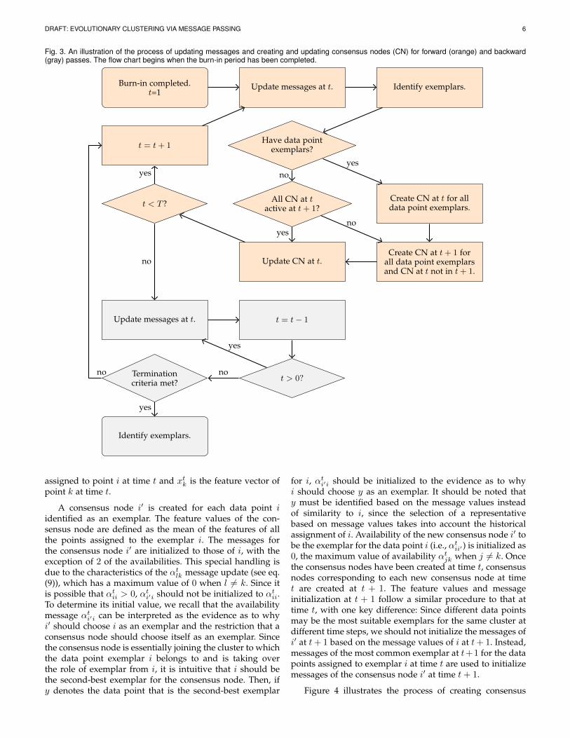
The process of performing message updates, consensusnode creation, and consensus node updates is illustrated inFigure 3. The forward pass is highlighted in orange whilethe backward pass is highlighted in gray. A consensus nodeis considered being active upon initialization and when itserves as an exemplar for data points. Consensus nodes areinactive before being born or after they have died.

To enable cluster tracking, messages are passed amongthe data points in the forward-backward fashion describedabove until at least 2 exemplars are identified in each timestep. This automatic burn-in period is necessary for theinitialization of the consensus node messages. At the endof the burn-in period, the data point exemplars at t = 1 areidentified and the consensus nodes created. The consensusnode creation is formalized by Algorithm 1 for the forwardpass of a single iteration, where eti denotes the exemplar

DRAFT: EVOLUTIONARY CLUSTERING VIA MESSAGE PASSING 6

Fig. 3. An illustration of the process of updating messages and creating and updating consensus nodes (CN) for forward (orange) and backward(gray) passes. The flow chart begins when the burn-in period has been completed.

Burn-in completed.t=1

Update messages at t. Identify exemplars.

Have data pointexemplars?

All CN at tactive at t+ 1?

Create CN at t for alldata point exemplars.

Create CN at t+ 1 forall data point exemplarsand CN at t not in t+ 1.

t = t+ 1

t < T ?

Update CN at t.

noyes

noyes

yes

Update messages at t. t = t− 1

t > 0?Terminationcriteria met?

Identify exemplars.

no

no

yes

no

yes

assigned to point i at time t and xtk is the feature vector ofpoint k at time t.

A consensus node i′ is created for each data point iidentified as an exemplar. The feature values of the con-sensus node are defined as the mean of the features of allthe points assigned to the exemplar i. The messages forthe consensus node i′ are initialized to those of i, with theexception of 2 of the availabilities. This special handling isdue to the characteristics of the αt

lk message update (see eq.(9)), which has a maximum value of 0 when l 6= k. Since itis possible that αt

ii > 0, αti′i should not be initialized to αt

ii.To determine its initial value, we recall that the availabilitymessage αt

i′i can be interpreted as the evidence as to whyi′ should choose i as an exemplar and the restriction that aconsensus node should choose itself as an exemplar. Sincethe consensus node is essentially joining the cluster to whichthe data point exemplar i belongs to and is taking overthe role of exemplar from i, it is intuitive that i should bethe second-best exemplar for the consensus node. Then, ify denotes the data point that is the second-best exemplar

for i, αti′i should be initialized to the evidence as to why

i should choose y as an exemplar. It should be noted thaty must be identified based on the message values insteadof similarity to i, since the selection of a representativebased on message values takes into account the historicalassignment of i. Availability of the new consensus node i′ tobe the exemplar for the data point i (i.e., αt

ii′ ) is initialized as0, the maximum value of availability αt

jk when j 6= k. Oncethe consensus nodes have been created at time t, consensusnodes corresponding to each new consensus node at timet are created at t + 1. The feature values and messageinitialization at t + 1 follow a similar procedure to that attime t, with one key difference: Since different data pointsmay be the most suitable exemplars for the same cluster atdifferent time steps, we should not initialize the messages ofi′ at t+ 1 based on the message values of i at t+ 1. Instead,messages of the most common exemplar at t+1 for the datapoints assigned to exemplar i at time t are used to initializemessages of the consensus node i′ at time t+ 1.

Figure 4 illustrates the process of creating consensus

DRAFT: EVOLUTIONARY CLUSTERING VIA MESSAGE PASSING 7

Algorithm 1 Cluster birth: Creation of consensus nodes

V t ← set of data points at time tCt ← set of consensus nodes at time tEt ← set of exemplars at time tfor i ∈ V t ∩ Et do:create consensus node i′ at time t:xti′ ←

∑j:etj=i x

ti

initialize message values of i′ to those of i:mt

i′j ← mtij ,m

tji′ ← mt

ji , for j∈ V t∪Ct,m∈{α, ρ, δ, φ}mt

i′i′ ← mtii , for m ∈ α, ρ, δ, φ

update αti′i and αt

ii′ :y ← argmaxj∈V t\i α

tij + ρtij + δtij + φtij

αti′i ← αt

iy

αtii′ ← 0

update exemplars to replace i with i′

end forinitialize consensus nodes at next time stepfor k ∈ Ct \ Ct+1 do:xt+1k ←

∑j:etj=k x

t+1j

l← argmaxj∈Et+1

∑i∈V t 1(eti = k)1(et+1

i = j)set messages for k at t + 1 using messages for l at t + 1following initialization of i′ messages aboveend for

nodes. In particular, the figure shows the status of group-ing data points represented by stacked polygons (squaresand triangles) following message updates at time t in theforward pass of EAP. The color of a polygon indicates theexemplar assigned to the corresponding data point whilethe shape of the polygons at both times reflects grouping ofthe corresponding points at time t. More specifically, thereare 2 exemplars at time t (red and blue) and 3 exemplars attime t+1 (purple, orange, and green). If both exemplars at tare data point exemplars, the algorithm creates 2 consensusnodes. The square consensus node at time t has a featurevector equal to the mean of the square data point featurevectors at time t and inherits message values α, ρ, δ, φ fromthe red exemplar at time t. The triangular consensus nodeat time t has a feature vector equal to the mean of thetriangular data point feature vectors at time t and inheritsmessage values α, ρ, δ, φ from the blue exemplar at timet. These consensus nodes are initialized at t + 1 beforeupdating the message values at that time step. The squareconsensus node at time t + 1 has a feature vector equal tothe mean of the square data point feature vectors at timet + 1 and inherits message values α, ρ, δ, φ from the mostcommon exemplar for the square data points at t + 1; inthis illustration, that is the orange exemplar. The triangularconsensus node at time t + 1 has a feature vector equalto the mean of the triangular data point feature vectors attime t + 1 and inherits message values α, ρ, δ, φ from themost common exemplar for the triangular data points att+1; here, the green exemplar. After the initialization of theconsensus nodes at t+ 1, the algorithm proceeds to updatemessages at t+ 1 including the new consensus nodes in themessage updates.

The creation of consensus nodes, and thus cluster births,occurs when data points are identified as exemplars. InEAP, exemplars are identified in the forward pass, at each

Fig. 4. An illustration how the consensus nodes are created. The stacksof polygons represent data points at times t and t + 1 after updatingthe messages at time t. The shape of a polygon indicates cluster mem-bership of the associated data point at time t while its color representsthe exemplar at the current time step; this is why at time t a color isconsistently associated with a polygon (i.e., all triangles are blue and allsquares are red). If the two exemplars at t are data points (as opposedto consensus nodes), a consensus node (CN) is created for each datapoint exemplar. These consensus nodes are further initialized at t + 1.At t, the square consensus node takes on a feature vector equal to themean of the square data points at t and has initial message values setto their exemplar (red) message values. At t+1, this square consensusnode is initialized with a data value equal to the mean of the square datapoints at t + 1. The message values for the square node at t + 1 areinitialized to the message values of the most common exemplar (mostcommon color, orange) from the square data points at t+ 1.

time step t, after the messages are updated. When the setof consensus nodes Ct is not empty, consensus nodes arefavored as exemplars. This is detailed in Algorithm 2, whereei indicates the exemplar for point i.

Algorithm 2 Exemplar identification

V t ← set of data points at time tCt ← set of consensus nodes at time tIdentify the set of exemplars E:E ← {j : αt

jj + ρtjj + δtjj + φtjj > 0}for i ∈ V t do

ECi ← {k ∈ E ∩ Ct : αtik + ρtik + δtik + φtik > 0}

if ECi 6= ∅ thenei ← argmaxk∈ECi α

tik + ρtik + δtik + φtik

elseei ← argmaxk∈E αt

ik + ρtik + δtik + φtikend if

end forreturn E ← E ∩ {e0, . . . , eN}

In order to track clusters, an additional update is per-formed during the exemplar identification and assignmentwhen a consensus node takes on a data point as an exem-

DRAFT: EVOLUTIONARY CLUSTERING VIA MESSAGE PASSING 8

plar. In the exemplar assignment, if a consensus node k doesnot identify itself as an exemplar but rather has data pointi as an exemplar, the consensus node takes on the messagevalues of i and the data points assigned to i as an exemplarare re-assigned to the consensus node k.

When an existing consensus node k is chosen as anexemplar (cluster evolution in Algorithm 3), the data valuefor k is updated as the mean of the data points that havek as the exemplar. After the data values are updated, thesimilarity matrix at time t is updated accordingly as well.

Algorithm 3 Cluster evolution and death via consensusnodesV t ← set of data points at time tCt ← set of consensus nodes at time tCt ← set of dead consensus nodes at time tidentify exemplars Et

Cluster evolutionfor k ∈ Ct ∩ Et do:xtk ←

∑j:etj=k x

tj

end forCluster deathCt ← Ct ∪ Ct \ Et

for t′ = t+ 1, . . . , T doCt′ ← Ct′ ∪ Ct \ Et

end for

If an existing consensus node is not selected as anexemplar, the cluster corresponding to the consensus node isconsidered to have died. Once a cluster has died, the samecluster cannot be born again in a future time step. Thereis an exception where a cluster may be “revived”, whicharises in the case of frequent change of exemplars beforethe message values converge. Suppose a consensus nodek dies at time t in iteration n. If the consensus node k isselected as an exemplar at time t − 1 in iteration n + 1, itis removed from the set of dead consensus nodes at t andits message values at t are re-established according to theinitialization in Algorithm 1. This process is repeated at t+1if the consensus node k is selected as an exemplar at time tin iteration n+ 1. The ability to revive a dead cluster whenmessage values at future iterations indicate evidence thatit should be active allows for a more accurate tracking ofclusters.

With particularly noisy data, it might be desirable torestrict creation and preservation of consensus nodes to onlythose clusters having size above a certain threshold. Settinga threshold may aid in finding a stable solution when, inthe initial iterations, many candidate exemplars are identi-fied. Since consensus nodes are preferred in the exemplarassignment, limiting the consensus nodes to a minimumcluster size discourages the assignment of data points totransitive consensus nodes or those that are representativeof outlier data. Note that such a restriction does not forcethe final solution to include only the clusters larger than thethreshold since data points may still emerge as exemplarsfor small clusters, including outliers that result in single-point clusters.

3.2 Effect of parameter valuesThe temporal smoothness and cluster tracking parametersintroduced in EAP, γ and ω, affect the number of clustersand the cluster memberships in the final result. In order tounderstand how to set the parameters, it is worth notingthat γ and ω affect the range of values that messages δ andφ can take on (as per eqs. (12) and (11)), such that if γ =ω = 0, then δtij = φtij = 0 for all i, j, t and the solution ofEAP without consensus nodes would be the same as that ofrunning AP separately at each time step.

In the case where γ = ω > 0, the δtij and φtij messages(where j is a consensus node) will be positive, and willin fact be the only non-zero messages. Note that from thedefinition of the function D in eq. (2), this is equivalent totreating solutions where data points are consistently chosenas exemplars in the same way as if a different exemplar waschosen at each time point. When γ > 0 and ω < γ, δtij andφtij can take on a maximum (positive) value of γ−ω for datapoints j or γ for consensus nodes j. Since consensus nodesare chosen as exemplars when αt

ij+ρtij+δ

tij+φ

tij > 0 for any

consensus node j in the set of exemplars, consensus nodesare more likely to be chosen as exemplars when γ > 0.

The value of ω should be set as a fraction of the valueof γ (i.e., ω = ξγ, ξ ∈ [0, 1]), where we have found thatξ ∈ [0, 0.5] yields good clustering results for real datasets.

Empirically, high values of γ may lead to a low numberof consensus nodes or clusters. This is due to the messagesδtij and φtij taking on a broader range of values, whichputs more weight on the temporal smoothness for exem-plar detection and assignment. The exemplar selection inturn affects the formation and survival of consensus nodes.Note that, typically, many consensus nodes are created afterthe burn-in period, and the number of consensus nodesdecreases as the message values stabilize. This is akin towhat is observed in classic AP, where fluctuating messagevalues lead to many more candidate exemplars in the earlieriterations than in the final solution. We have observedthat high values of the ratio ω/γ may lead to two typesof detrimental effects, resulting in either too few or toomany consensus nodes. If the number of consensus nodescreated immediately after the burn-in is not sufficientlylarge, the creation of new clusters may be discouraged andthe clustering solution will have too few clusters. With highω/γ, another possibility is that too many exemplars willbe identified, and thus too many consensus nodes will becreated. Moreover, high value of ω/γ makes it more likelythat more consensus nodes will continue being selected asexemplars as the message values iterate, possibly resultingin poor tracking or in a higher than optimal number ofclusters in the final solution. Thus, we recommend a lowvalue of ω as stated above (i.e., ω = ξγ, ξ ∈ [0, 0.5]).

3.3 Insertion and deletion of time pointsEAP is capable of handling datasets where data points arenot present for the entire duration of the considered timehorizon; in such scenarios, EAP tracks the set of “active”data points Vt at each time step t and only passes messagesbetween the active data points and active consensus nodes.If a data point i is inserted at time t, i ∈ V t, i 6∈ V t−1,the messages are initialized in a manner similar to the

DRAFT: EVOLUTIONARY CLUSTERING VIA MESSAGE PASSING 9

message update in the incremental AP [32]. For such a datapoint i, the nearest neighbor k1 in the set of active datapoints at time t is identified as k1 = argmaxj∈V t\i s

tij .

During each EAP iteration, at time t in the forward step, themessages for the inserted data points are initialized to thoseof their nearest neighbors. Unlike the message initializationfor inserted points in [32], EAP requires an additional stepfor updating availabilities of the inserted data points inorder to avoid violating the requirement that αt

ij ≤ 0 wheni 6= j. To avoid αt

ik1> 0, the availability messages of interest

are initialized based on the message values of the secondnearest-neighbor k2 such that αt

ik1= αt

k2k1, αt

k1i= αt

k1k2.

Finally, the messages from i to itself (e.g. αtii) are initialized

to the message values from k1 to itself.In the case of a data point deletion at time t, the only

action needed is the removal of the data point from the setof active nodes at time t.

4 EXPERIMENTAL RESULTS

We test EAP on several synthetic datasets as well as realdatasets comprising ocean and stock data. In the EAPand AP implementations, the similarity between points isdefined as the negative squared Euclidean distance. Thepreference (self-similarity) is set to the minimum similar-ity between all data points at a given time step for eachsynthetic and real dataset. We compare the performanceof EAP to that of the AFFECT’s evolutionary spectralclustering framework [3], as well as to the classic (static)AP. AFFECT was implemented using the AFFECT Matlabtoolbox. For clustering the synthetic and real ocean datawith AFFECT, the similarity between xi and xj is definedas exp(−‖xi − xj‖22/2σ2), with the default value 2σ2 = 5.Note that even though the AFFECT framework should inprinciple be capable of employing any similarity metric [3],we chose to compute the similarities based on the Gaussiankernel for use in the AFFECT framework since that providessignificantly better on the synthetic and ocean datasets thanrunning the framework with similarities defined as thenegative squared Euclidean distance (i.e., the similaritiesused by EAP and AP). The negative squared Euclideandistance is used as a similarity metric for all algorithmsapplied to the analysis of the stock dataset. To determinethe number of clusters needed to run AFFECT, we used themodularity criterion [33] since it allows for varying numberof clusters across time and performs better than the alterna-tive approach where the number of clusters is determinedby maximizing the silhouette width [34]. Note that theAFFECT framework was previously shown to outperformevolutionary k-means, evolutionary spectral clustering, andthe framework proposed by Rosswog and Ghose [13] onvarious synthetic and real datasets.

Clustering accuracy is evaluated by means of the Randindex [35] when data labels are available. The Rand index isdefined as the percentage of pairs of points that are correctlyclassified as being either in the same cluster or in differentclusters.

4.1 Gaussian dataWe test our algorithm on four Gaussian mixture modelsused to generate the synthetic datasets in [3], each with 2-

TABLE 1Accuracy Expressed in Terms of Rand Index for Gaussian Datasets

Dataset EAP AP EAP:noCN AFFECTseparated Gaussians 1 1 1 1colliding Gaussians 1 0.943 0.990 1

cluster change 0.998 0.879 0.981 0.964third cluster 0.999 0.971 0.999 0.963

dimensional Gaussians and 200 data points. The componentmembership for each data point is set and does not changeover time unless specified otherwise. The initial mixtureweights are uniform. At each time step, points in each of thecomponents are drawn from the corresponding Gaussiandistribution. The first dataset consists of two well-separatedGaussians and 40 time steps. The means at the initial timestep are set to [−4, 0] and [4, 0], with the covariance of 0.1I(I denotes the identity matrix). At each time step, the firstdimension of the mean of each component is altered by arandom walk with step size 0.1. At the time step 19, thecovariance matrix is changed to 0.3I . The second datasetis generated from two colliding Gaussians with the initialmeans of [−3,−3] and [3, 3] and identity covariance. Ineach of the time instances t = 2, . . . , 9, the mean of thefirst component is increased by [0.4, 0.4]. From t = 10 tot = 25, the means remain constant and the data pointsare drawn from their respective mixture component. Thethird dataset is generated in a similar way as the secondone, with the difference that some points change clusters.In particular, at time steps t = 10 and t = 11, points inthe second component switch to the first component witha probability of 0.25, altering the mixture weights. Fromt = 12 to t = 25, the data points maintain the componentmembership they had at t = 11. Finally, the fourth datasetis generated the same way as the second one for the first9 time steps. For t = 10 and t = 11, data points in thesecond cluster switch membership with a probability of 0.25to a new third Gaussian component with mean [−3,−3] andidentity covariance.

In addition to the comparison with the AFFECT’s evo-lutionary spectral clustering framework, the EAP resultsare compared with those achieved by clustering with APindependently at each time step. In order to demonstratethe impact of the consensus nodes on performance, we alsocompare the results with an implementation of evolutionaryaffinity propagation that does not employ consensus nodesand has message updates equivalent to those of EAP withω = 0. The results of EAP and its no-consensus-nodes vari-ant labeled EAP:noCN are shown in Table 1. The parametersfor the colliding Gaussians with a third cluster dataset wereset to γ = 5 and ω = 2, while for the other Gaussian datasetsthe parameters are γ = 5 and ω = 1. It should be noted thatrunning EAP with γ = 5 and ω = 1 on the dataset with athird cluster yielded a clustering solution with Rand indexof 0.997. The corresponding numbers of distinct exemplarsacross the time steps are shown in Table 2.

EAP achieved near-perfect clustering and correctlytracked clusters for all 4 datasets. Clustering with the EAPmessages but without consensus nodes yielded more ac-curate results and tracked clusters better than individually

DRAFT: EVOLUTIONARY CLUSTERING VIA MESSAGE PASSING 10

TABLE 2The Number of Distinct Exemplars for Gaussian Datasets

Dataset EAP AP EAP:noCNseparated Gaussians 2 67 22colliding Gaussians 2 48 11

cluster change 2 51 11third cluster 3 58 18

clustering with AP at every time step, resulting in a higherRand index and lower number of distinct exemplars thanAP. However, the accuracy of EAP:noCN was lower thanthat of EAP. This can be attributed to the competing exem-plars at consecutive time steps. Specifically, when severaldata points are potentially good exemplars for a cluster, themessage dependence on the future and past time steps mayresult in more candidate exemplars at a single time stepthan if the clustering were solely performed based on thedata collected in that time step. Despite the Rand index ofEAP:noCN being higher than that of AP due to incorporat-ing temporal smoothness, at times the competing exemplarsresult in a higher than actual number of clusters. The inclu-sion of consensus nodes and the message initialization andupdates in EAP overcome this limitation of EAP:noCN. Inthe dataset with points forming a third cluster, both EAPand EAP:noCN achieve near-perfect clustering. However,EAP (Rand index = 0.9998) slightly outperforms its coun-terpart without the consensus nodes (Rand index = 0.9991),misclassifying just a single point when the third clusteris introduced at t = 10. EAP outperforms AFFECT withspectral clustering for the datasets having points changingclusters and points forming a third separate cluster, provid-ing significantly higher accuracy during the 4 and 8 timesteps, respectively, following the initial cluster membershipchange. In the case of the additional cluster, AFFECT doesnot detect the third cluster until time step 18 even though itwas formed in time step 10; as a consequence, its Rand indexis lower than that of AP applied independently at individualtime steps. This highlights the advantage of automaticallyidentifying the number of clusters at each time step in EAPand avoiding heuristics used by other methods includingAFFECT.

Fig. 5. Rand index for colliding Gaussians with the change in clustermembership (left) and the appearance of a third cluster (right).

0 10 20

t

0.6

0.7

0.8

0.9

1

Rand i

ndex

0 10 20

t

0.6

0.7

0.8

0.9

1

AP

EAP:noCN

AFFECT

EAP

Figure 5 shows the Rand index across time steps forthe colliding Gaussians with some points changing clustermembership at times t ∈ {10, 11} (left panel) and collidingGaussians with some points switching to a new third clusterat t ∈ {10, 11} (right panel). In both datasets, as the datapoints from the two Gaussians get closer, the Rand index forAP (green) begins to drop. When the cluster membershipis altered, such that a third cluster is introduced or datapoints switch cluster membership, the Rand index for APdrops further. The case where points switch cluster mem-bership results in a lower Rand index for AP since somedata points exhibit closer similarities to points from theother cluster and AP cannot correct the clustering based onthe data points’ history. As mentioned above, without theintroduction of consensus nodes (EAP:noCN, black), someexemplars may compete against each other and the numberof clusters may be overestimated, resulting in a lower Randindex for t ∈ {9, 14}. EAP (red) yields the best clusteringresults, with a slight decrease in the Rand index aroundthe time of the perturbation in the cluster membershipsfollowed by a quick recovery.

4.2 Real (experimental) data

We tested the proposed evolutionary clustering algorithmon two real data sets: ocean temperature and salinity dataat the location where the Atlantic Ocean meets the IndianOcean, and stock prices from the first half of the year 2000.

4.2.1 Ocean water massesArgo, an ocean observation system, has enabled trackingof ocean temperature and salinity since 2000. More than3900 floats currently in the Argo network cycle between theocean surface and 2000m depth every 10 days, providingsalinity and temperature measurements at varying depths.The primary goal of the Argo program is to aid in the under-standing of climate variability. Evolutionary clustering pro-vides a way to discover and track changes in water massesat different depths. A water mass is a body of water witha common formation and homogenous values of variousfeatures, such as temperature and salinity, within it. Studyof water masses can provide insight into climate change,seasonal climatological variations, ocean biogeochemistry,and ocean circulation and its effect on transport of oxygenand organisms, which in turn affects the biological diversityof an area. Clustering has previously been used to identifywater masses with datasets comprising temperature, salin-ity, chemical, and optical measurements [36], [37], [38], [39],[40]. However, in studies that explore seasonal variationsof water masses, clustering is performed independently atdifferent time points of interest and the results for differentseasons are compared in order to find variations [38], [39],[40].

We examine the data from the Roemmich-Gilson (RG)Argo Climatology [41] which contains monthly averages(since January 2004) of ocean temperature and salinity datawith a 1 degree resolution worldwide.

Clustering is performed on the temperature and salinitydata at the location near the coast of South Africa wherethe Indian Ocean meets the South Atlantic. Specifically, thedata is obtained from the latitudes 25◦ S to 55◦ S and

DRAFT: EVOLUTIONARY CLUSTERING VIA MESSAGE PASSING 11

Fig. 6. Water masses at 1000 dbar. Clustering results for EAP (left), AP (middle), and AFFECT (right) at t = 2 (top) and t = 3 (bottom) are shown.

������ �� �������

������ ��� ��� ��� �� ��� ���

������

������

� ��� ��� �� ��� ���

�����

����������

� ��� ��� �� ��� ���

���������

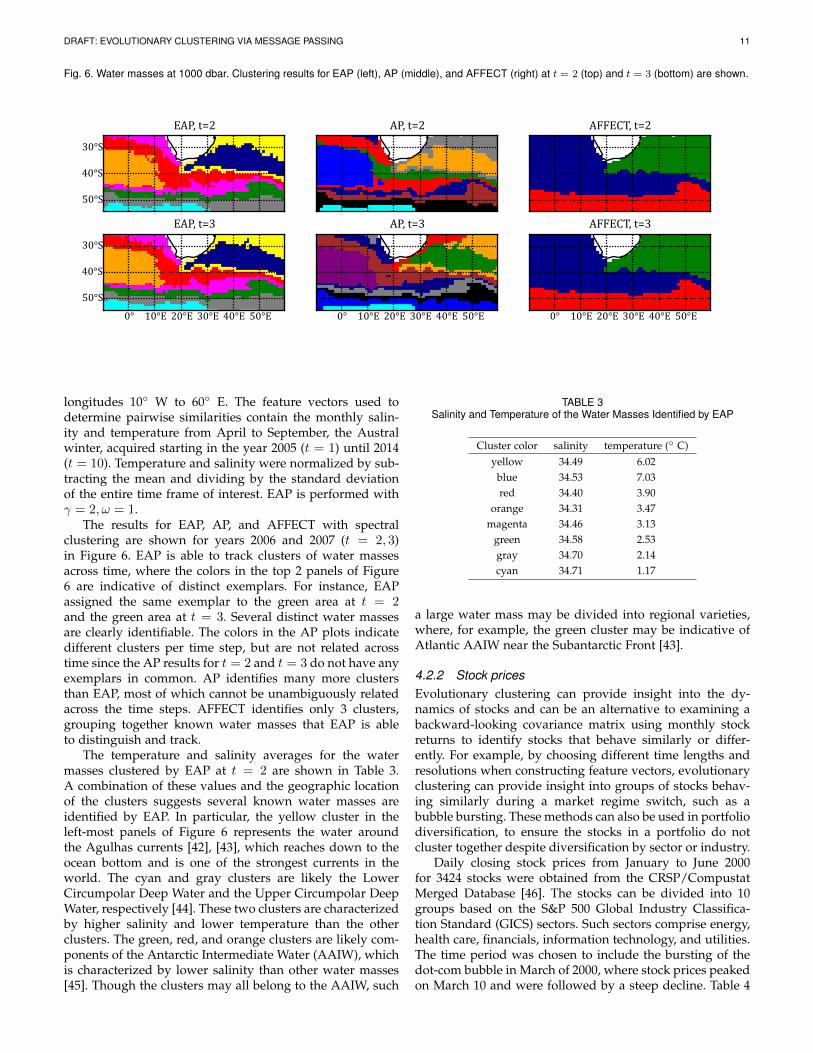
longitudes 10◦ W to 60◦ E. The feature vectors used todetermine pairwise similarities contain the monthly salin-ity and temperature from April to September, the Australwinter, acquired starting in the year 2005 (t = 1) until 2014(t = 10). Temperature and salinity were normalized by sub-tracting the mean and dividing by the standard deviationof the entire time frame of interest. EAP is performed withγ = 2, ω = 1.

The results for EAP, AP, and AFFECT with spectralclustering are shown for years 2006 and 2007 (t = 2, 3)in Figure 6. EAP is able to track clusters of water massesacross time, where the colors in the top 2 panels of Figure6 are indicative of distinct exemplars. For instance, EAPassigned the same exemplar to the green area at t = 2and the green area at t = 3. Several distinct water massesare clearly identifiable. The colors in the AP plots indicatedifferent clusters per time step, but are not related acrosstime since the AP results for t = 2 and t = 3 do not have anyexemplars in common. AP identifies many more clustersthan EAP, most of which cannot be unambiguously relatedacross the time steps. AFFECT identifies only 3 clusters,grouping together known water masses that EAP is ableto distinguish and track.

The temperature and salinity averages for the watermasses clustered by EAP at t = 2 are shown in Table 3.A combination of these values and the geographic locationof the clusters suggests several known water masses areidentified by EAP. In particular, the yellow cluster in theleft-most panels of Figure 6 represents the water aroundthe Agulhas currents [42], [43], which reaches down to theocean bottom and is one of the strongest currents in theworld. The cyan and gray clusters are likely the LowerCircumpolar Deep Water and the Upper Circumpolar DeepWater, respectively [44]. These two clusters are characterizedby higher salinity and lower temperature than the otherclusters. The green, red, and orange clusters are likely com-ponents of the Antarctic Intermediate Water (AAIW), whichis characterized by lower salinity than other water masses[45]. Though the clusters may all belong to the AAIW, such

TABLE 3Salinity and Temperature of the Water Masses Identified by EAP

Cluster color salinity temperature (◦ C)yellow 34.49 6.02

blue 34.53 7.03red 34.40 3.90

orange 34.31 3.47magenta 34.46 3.13

green 34.58 2.53gray 34.70 2.14cyan 34.71 1.17

a large water mass may be divided into regional varieties,where, for example, the green cluster may be indicative ofAtlantic AAIW near the Subantarctic Front [43].

4.2.2 Stock pricesEvolutionary clustering can provide insight into the dy-namics of stocks and can be an alternative to examining abackward-looking covariance matrix using monthly stockreturns to identify stocks that behave similarly or differ-ently. For example, by choosing different time lengths andresolutions when constructing feature vectors, evolutionaryclustering can provide insight into groups of stocks behav-ing similarly during a market regime switch, such as abubble bursting. These methods can also be used in portfoliodiversification, to ensure the stocks in a portfolio do notcluster together despite diversification by sector or industry.

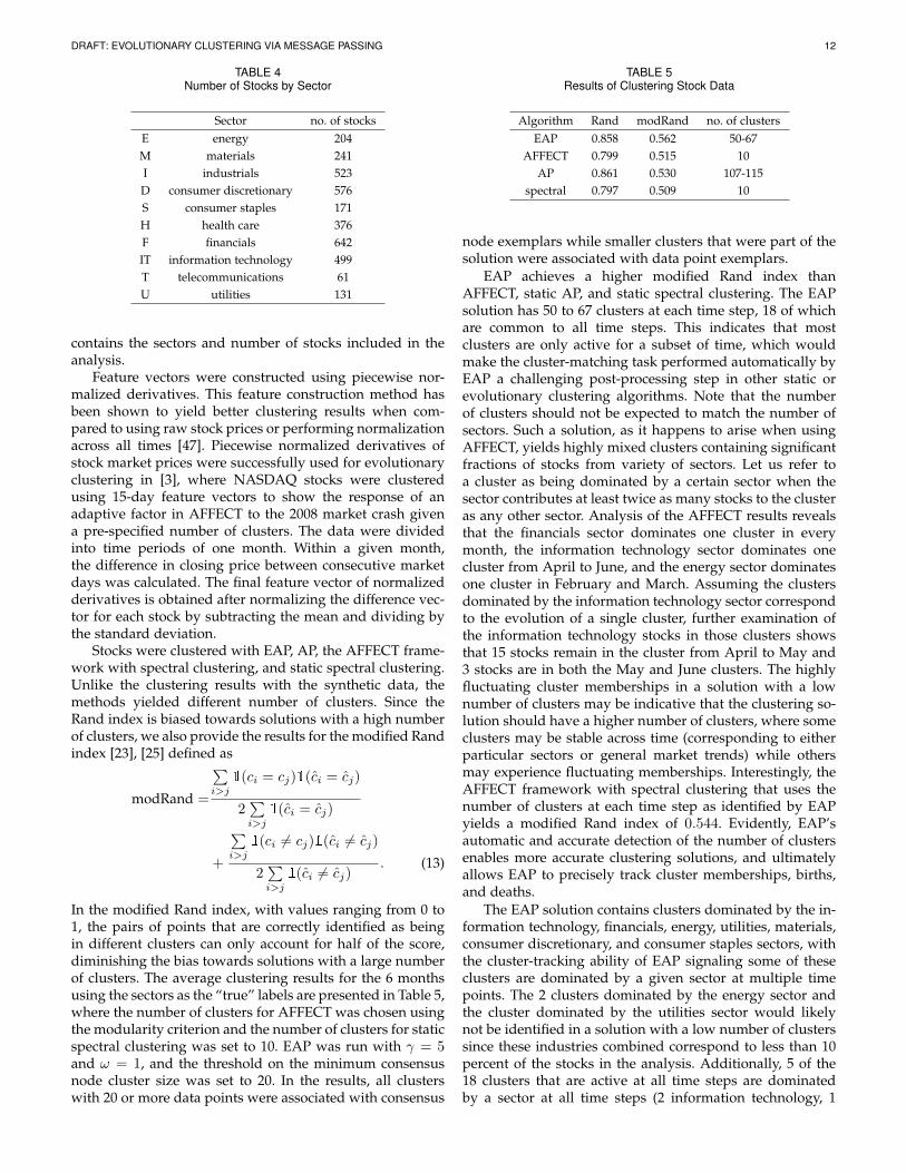
Daily closing stock prices from January to June 2000for 3424 stocks were obtained from the CRSP/CompustatMerged Database [46]. The stocks can be divided into 10groups based on the S&P 500 Global Industry Classifica-tion Standard (GICS) sectors. Such sectors comprise energy,health care, financials, information technology, and utilities.The time period was chosen to include the bursting of thedot-com bubble in March of 2000, where stock prices peakedon March 10 and were followed by a steep decline. Table 4

DRAFT: EVOLUTIONARY CLUSTERING VIA MESSAGE PASSING 12

TABLE 4Number of Stocks by Sector

Sector no. of stocksE energy 204M materials 241I industrials 523D consumer discretionary 576S consumer staples 171H health care 376F financials 642IT information technology 499T telecommunications 61U utilities 131

contains the sectors and number of stocks included in theanalysis.

Feature vectors were constructed using piecewise nor-malized derivatives. This feature construction method hasbeen shown to yield better clustering results when com-pared to using raw stock prices or performing normalizationacross all times [47]. Piecewise normalized derivatives ofstock market prices were successfully used for evolutionaryclustering in [3], where NASDAQ stocks were clusteredusing 15-day feature vectors to show the response of anadaptive factor in AFFECT to the 2008 market crash givena pre-specified number of clusters. The data were dividedinto time periods of one month. Within a given month,the difference in closing price between consecutive marketdays was calculated. The final feature vector of normalizedderivatives is obtained after normalizing the difference vec-tor for each stock by subtracting the mean and dividing bythe standard deviation.

Stocks were clustered with EAP, AP, the AFFECT frame-work with spectral clustering, and static spectral clustering.Unlike the clustering results with the synthetic data, themethods yielded different number of clusters. Since theRand index is biased towards solutions with a high numberof clusters, we also provide the results for the modified Randindex [23], [25] defined as

modRand =

∑i>j

1(ci = cj)1(ci = cj)

2∑i>j

1(ci = cj)

+

∑i>j

1(ci 6= cj)1(ci 6= cj)

2∑i>j

1(ci 6= cj). (13)

In the modified Rand index, with values ranging from 0 to1, the pairs of points that are correctly identified as beingin different clusters can only account for half of the score,diminishing the bias towards solutions with a large numberof clusters. The average clustering results for the 6 monthsusing the sectors as the “true” labels are presented in Table 5,where the number of clusters for AFFECT was chosen usingthe modularity criterion and the number of clusters for staticspectral clustering was set to 10. EAP was run with γ = 5and ω = 1, and the threshold on the minimum consensusnode cluster size was set to 20. In the results, all clusterswith 20 or more data points were associated with consensus

TABLE 5Results of Clustering Stock Data

Algorithm Rand modRand no. of clustersEAP 0.858 0.562 50-67

AFFECT 0.799 0.515 10AP 0.861 0.530 107-115

spectral 0.797 0.509 10

node exemplars while smaller clusters that were part of thesolution were associated with data point exemplars.

EAP achieves a higher modified Rand index thanAFFECT, static AP, and static spectral clustering. The EAPsolution has 50 to 67 clusters at each time step, 18 of whichare common to all time steps. This indicates that mostclusters are only active for a subset of time, which wouldmake the cluster-matching task performed automatically byEAP a challenging post-processing step in other static orevolutionary clustering algorithms. Note that the numberof clusters should not be expected to match the number ofsectors. Such a solution, as it happens to arise when usingAFFECT, yields highly mixed clusters containing significantfractions of stocks from variety of sectors. Let us refer toa cluster as being dominated by a certain sector when thesector contributes at least twice as many stocks to the clusteras any other sector. Analysis of the AFFECT results revealsthat the financials sector dominates one cluster in everymonth, the information technology sector dominates onecluster from April to June, and the energy sector dominatesone cluster in February and March. Assuming the clustersdominated by the information technology sector correspondto the evolution of a single cluster, further examination ofthe information technology stocks in those clusters showsthat 15 stocks remain in the cluster from April to May and3 stocks are in both the May and June clusters. The highlyfluctuating cluster memberships in a solution with a lownumber of clusters may be indicative that the clustering so-lution should have a higher number of clusters, where someclusters may be stable across time (corresponding to eitherparticular sectors or general market trends) while othersmay experience fluctuating memberships. Interestingly, theAFFECT framework with spectral clustering that uses thenumber of clusters at each time step as identified by EAPyields a modified Rand index of 0.544. Evidently, EAP’sautomatic and accurate detection of the number of clustersenables more accurate clustering solutions, and ultimatelyallows EAP to precisely track cluster memberships, births,and deaths.

The EAP solution contains clusters dominated by the in-formation technology, financials, energy, utilities, materials,consumer discretionary, and consumer staples sectors, withthe cluster-tracking ability of EAP signaling some of theseclusters are dominated by a given sector at multiple timepoints. The 2 clusters dominated by the energy sector andthe cluster dominated by the utilities sector would likelynot be identified in a solution with a low number of clusterssince these industries combined correspond to less than 10percent of the stocks in the analysis. Additionally, 5 of the18 clusters that are active at all time steps are dominatedby a sector at all time steps (2 information technology, 1

DRAFT: EVOLUTIONARY CLUSTERING VIA MESSAGE PASSING 13

financials, 1 energy, 1 utilities). As in the case of AFFECT,cluster memberships change over time, with between 42and 76 percent of the stocks remaining in the same clusterthrough consecutive months.

Fig. 7. EAP cluster membership by sector. The sectors are listed onthe horizontal axis, with the vertical axis corresponding to the clusters.The color indicates participation of a sector in a given cluster in termsof percentage of the cluster’s size, with red corresponding to higherpercentage. Blank rows indicate clusters that are not active. The sectorlabels are defined in Table 4.

E M I D S H F IT T U

February

E M I D S H F IT T U

March

E M I D S H F IT T U

April

A significant change in the structure of clusters occursbetween February and March, the months containing 55 and67 clusters, respectively. In Figure 7, each panel correspondsto a time step in EAP, the horizontal axis corresponds tothe sectors (Table 4), and each row corresponds to a specificcluster tracked across time, with blank rows indicating inac-tive clusters. The color represents the percentage of the clus-ter that belongs to a given sector, with red indicating higherpercentage. The active clusters undergo a major changebetween February and March and remain more consistentbetween March and April, suggesting a reorganization inMarch. The sector-dominated clusters can be identified inFigure 7 by observing locations of red rectangles, and theirdynamics can be tracked. For instance, it can be seen that theclusters dominated by utilities (U) and energy (E) sectors areconsistent across time, and that the cluster re-organization inMarch results in a second energy-dominated cluster whosestructure remains preserved through April. The numerouscluster births and deaths illustrated in Figure 7 further em-phasize advantages of automatic cluster number detectionand cluster tracking that are among EAP’s features.

5 CONCLUSION

We developed an evolutionary clustering algorithm, evolu-tionary affinity propagation (EAP), which groups points bypassing messages on a factor graph. The EAP graph includesfactors connecting variable nodes across time, inducing tem-poral smoothness. We introduce the concept of consensusnodes and describe message initialization and updates thatencourage data points to choose an existing consensus nodeas their exemplar. Through these nodes, we can identifycluster births and deaths as well as track the clusters acrosstime. EAP outperforms an evolutionary spectral clustering

algorithm as well as the individual time step clusteringby AP on several Gaussian mixture models emulating cir-cumstances such as changes in cluster membership and theemergence of an additional cluster. When applied to anocean water dataset, EAP was able to identify known watermasses and automatically match the discovered clustersacross time. In a stock clustering application, EAP yields amore accurate and interpretable solution than existing staticand evolutionary clustering methods. EAP’s capability toidentify the number of clusters and perform cluster trackingwithout additional pre- or post-processing steps makes it adesirable algorithm for studying the evolution of clusterswhen data is acquired at multiple time steps, such as in thestudy of climate change or exploration of social networks.

ACKNOWLEDGMENTS

This work was supported by the NSF Graduate ResearchFellowship grant DGE-1110007. The authors would like tothank Isabella Arzeno for her oceanography advice on watermass clustering, ranging from the suggestion of the problemand dataset to the interpretation of the results.

REFERENCES

[1] D. Chakrabarti, R. Kumar, and A. Tomkins, “Evolutionary clus-tering,” in Proceedings of the 12th ACM SIGKDD International Con-ference on Knowledge Discovery and Data Mining. New York, NY,USA: ACM, 2006, pp. 554–560.

[2] A. Ahmed and E. Xing, “Dynamic non-parametric mixture modelsand the recurrent chinese restaurant process: with applicationsto evolutionary clustering,” in Proceedings of the 2008 SIAM In-ternational Conference on Data Mining. Society for Industrial andApplied Mathematics, Apr. 2008, pp. 219–230.

[3] K. S. Xu, M. Kliger, and A. O. Hero III, “Adaptive evolutionaryclustering,” Data Mining and Knowledge Discovery, vol. 28, no. 2,pp. 304–336, Jan. 2013.

[4] Y. Chi, X. Song, D. Zhou, K. Hino, and B. L. Tseng, “Evolutionaryspectral clustering by incorporating temporal smoothness,” inProceedings of the 13th ACM SIGKDD International Conference onKnowledge Discovery and Data Mining. New York, NY, USA: ACM,2007, pp. 153–162.

[5] ——, “On evolutionary spectral clustering,” ACM Trans. Knowl.Discov. Data, vol. 3, no. 4, pp. 17:1–17:30, Dec. 2009.

[6] K. S. Xu, M. Kliger, and A. O. Hero III, “Tracking communities ofspammers by evolutionary clustering,” in International Conferenceon Machine Learning Workshop on Social Analytics: Learning fromHuman Interactions, 2010.

[7] E. P. X. Amr Ahmed, “Timeline: A dynamic hierarchical dirichletprocess model for recovering birth/death and evolution of topicsin text stream,” in Proceedings of the Twenty-Sixth Conference onUncertainty in Artificial Intelligence, 2010, pp. 20–29.

[8] T. Xu, Z. Zhang, P. Yu, and B. Long, “Evolutionary clustering byhierarchical dirichlet process with hidden markov state,” in EighthIEEE International Conference on Data Mining, 2008. ICDM ’08, Dec.2008, pp. 658–667.

[9] F. Folino and C. Pizzuti, “An evolutionary multiobjective approachfor community discovery in dynamic networks,” IEEE Transactionson Knowledge and Data Engineering, vol. 26, no. 8, pp. 1838–1852,Aug. 2014.

[10] N. Czink, R. Tian, S. Wyne, F. Tufvesson, J.-P. Nuutinen, J. Ylitalo,E. Bonek, and A. Molisch, “Tracking time-variant cluster param-eters in MIMO channel measurements,” in Second InternationalConference on Communications and Networking in China, 2007., Aug.2007, pp. 1147–1151.

[11] S. Gunnemann, H. Kremer, C. Laufkotter, and T. Seidl, “Tracingevolving subspace clusters in temporal climate data,” Data Miningand Knowledge Discovery, vol. 24, no. 2, pp. 387–410, Sep. 2011.

[12] Y. Wang, S. Liu, J. Feng, and L. Zhou, “Mining naturally smoothevolution of clusters from dynamic data,” in Proceedings of the2007 SIAM International Conference on Data Mining. Society forIndustrial and Applied Mathematics, Apr. 2007, pp. 125–134.

DRAFT: EVOLUTIONARY CLUSTERING VIA MESSAGE PASSING 14

[13] J. Rosswog and K. Ghose, “Detecting and tracking spatio-temporalclusters with adaptive history filtering,” in IEEE InternationalConference on Data Mining Workshops, Dec. 2008, pp. 448–457.

[14] Y.-M. Kim, J. Velcin, S. Bonnevay, and M.-A. Rizoiu, “Temporalmultinomial mixture for instance-oriented evolutionary cluster-ing,” in Advances in Information Retrieval, ser. Lecture Notes inComputer Science, A. Hanbury, G. Kazai, A. Rauber, and N. Fuhr,Eds. Springer International Publishing, Mar. 2015, no. 9022, pp.593–604.

[15] X. Jia, N. Du, J. Gao, and A. Zhang, “Analysis on community vari-ational trend in dynamic networks,” in Proceedings of the 23rd ACMInternational Conference on Conference on Information and KnowledgeManagement. New York, NY, USA: ACM, 2014, pp. 151–160.

[16] T. Yang, Y. Chi, S. Zhu, Y. Gong, and R. Jin, “Detecting communi-ties and their evolutions in dynamic social networks—a Bayesianapproach,” Machine Learning, vol. 82, no. 2, pp. 157–189, Sep. 2010.

[17] S. Fortunato, “Community detection in graphs,” Physics Reports,vol. 486, no. 3–5, pp. 75–174, Feb. 2010.

[18] S. Papadopoulos, Y. Kompatsiaris, A. Vakali, and P. Spyridonos,“Community detection in social media,” Data Mining and Knowl-edge Discovery, vol. 24, no. 3, pp. 515–554, Jun. 2011.

[19] M.-S. Kim and J. Han, “A particle-and-density based evolutionaryclustering method for dynamic networks,” Proc. VLDB Endow.,vol. 2, no. 1, pp. 622–633, Aug. 2009.

[20] B. J. Frey and D. Dueck, “Clustering by passing messages betweendata points,” Science, vol. 315, no. 5814, pp. 972–976, Feb. 2007.

[21] I. E. Givoni and B. J. Frey, “A binary variable model for affinitypropagation,” Neural computation, vol. 21, no. 6, pp. 1589–1600,Jun. 2009.

[22] D. Dueck and B. Frey, “Non-metric affinity propagation for unsu-pervised image categorization,” in IEEE 11th International Confer-ence on Computer Vision, 2007., Oct. 2007, pp. 1–8.

[23] I. E. Givoni and B. J. Frey, “Semi-supervised affinity propagationwith instance-level constraints,” in Proceedings of the Twelfth Inter-national Conference on Artificial Intelligence and Statistics, 2009, pp.161–168.

[24] M. Leone, Sumedha, and M. Weigt, “Unsupervised and semi-supervised clustering by message passing: soft-constraint affinitypropagation,” The European Physical Journal B, vol. 66, no. 1, pp.125–135, Oct. 2008.

[25] N. M. Arzeno and H. Vikalo, “Semi-supervised affinity propa-gation with soft instance-level constraints,” IEEE Transactions onPattern Analysis and Machine Intelligence, vol. 37, no. 5, pp. 1041–1052, May 2015.

[26] M. Leone, Sumedha, and M. Weigt, “Clustering by soft-constraintaffinity propagation: applications to gene-expression data,” Bioin-formatics, vol. 23, no. 20, pp. 2708–2715, Oct. 2007.

[27] I. Givoni, C. Chung, and B. J. Frey, “Hierarchical affinity propaga-tion,” arXiv e-print 1202.3722, Feb. 2012.

[28] C.-D. Wang, J.-H. Lai, C. Y. Suen, and J.-Y. Zhu, “Multi-exemplaraffinity propagation,” IEEE Transactions on Pattern Analysis andMachine Intelligence, Jan. 2013.

[29] Y. Fujiwara, M. Nakatsuji, H. Shiokawa, Y. Ida, and M. Toy-oda, “Adaptive message update for fast affinity propagation,” inProceedings of the 21th ACM SIGKDD International Conference onKnowledge Discovery and Data Mining. New York, NY, USA: ACM,2015, pp. 309–318.

[30] V. Quera, F. S. Beltran, I. E. Givoni, and R. Dolado, “Determiningshoal membership using affinity propagation,” Behavioural BrainResearch, vol. 241, pp. 38–49, Mar. 2013.

[31] C. M. Bishop, Pattern Recognition and Machine Learning. Springer,Aug. 2006.

[32] L. Sun and C. Guo, “Incremental affinity propagation clusteringbased on message passing,” IEEE Transactions on Knowledge andData Engineering, vol. 26, no. 11, pp. 2731–2744, 2014.

[33] M. E. J. Newman, “Modularity and community structure in net-works,” Proceedings of the National Academy of Sciences, vol. 103,no. 23, pp. 8577–8582, Jun. 2006.

[34] P. J. Rousseeuw, “Silhouettes: A graphical aid to the interpretationand validation of cluster analysis,” Journal of Computational andApplied Mathematics, vol. 20, pp. 53–65, Nov. 1987.

[35] W. M. Rand, “Objective criteria for the evaluation of clusteringmethods,” Journal of the American Statistical Association, vol. 66, no.336, pp. 846–850, Dec. 1971.

[36] M. J. Oliver, S. Glenn, J. T. Kohut, A. J. Irwin, O. M. Schofield,M. A. Moline, and W. P. Bissett, “Bioinformatic approaches for ob-

jective detection of water masses on continental shelves,” Journal ofGeophysical Research: Oceans, vol. 109, no. C7, p. C07S04, Jul. 2004.

[37] S. M. Techtmann, J. L. Fortney, K. A. Ayers, D. C. Joyner, T. D.Linley, S. M. Pfiffner, and T. C. Hazen, “The unique chemistry ofEastern Mediterranean water masses selects for distinct microbialcommunities by depth,” PLoS ONE, vol. 10, no. 3, Mar. 2015.

[38] S. Yusong, Y. Zuxiang, and L. Fengqi, “Application of the clus-tering method in analysing shallow water masses and modifiedwater masses in the Huanghai Sea and East China Sea,” ChineseJournal of Oceanology and Limnology, vol. 1, no. 3, pp. 272–284, Dec.1983.

[39] S. Chen, Y. Li, J. Hu, A. Zheng, L. Huang, and Y. Lin, “Multipa-rameter cluster analysis of seasonal variation of water masses inthe eastern Beibu Gulf,” Journal of Oceanography, vol. 67, no. 6, pp.709–718, Oct. 2011.

[40] J. Qi, B. Yin, Q. Zhang, D. Yang, and Z. Xu, “Analysis of seasonalvariation of water masses in East China Sea,” Chinese Journal ofOceanology and Limnology, vol. 32, no. 4, pp. 958–971, Jul. 2014.

[41] D. Roemmich and J. Gilson, “The 2004–2008 mean and annualcycle of temperature, salinity, and steric height in the global oceanfrom the Argo Program,” Progress in Oceanography, vol. 82, no. 2,pp. 81–100, Aug. 2009.

[42] L. D. Talley, G. L. Pickard, W. J. Emery, and J. H. Swift, “Chapter11 - Indian Ocean,” in Descriptive Physical Oceanography (SixthEdition). Boston: Academic Press, 2011, pp. 363–399.

[43] E. Rusciano, S. Speich, and M. Ollitrault, “Interocean exchangesand the spreading of Antarctic Intermediate Water south ofAfrica,” Journal of Geophysical Research: Oceans, vol. 117, no. C10,p. C10010, Oct. 2012.

[44] L. D. Talley, G. L. Pickard, W. J. Emery, and J. H. Swift, “Chapter13 - Southern Ocean,” in Descriptive Physical Oceanography (SixthEdition). Boston: Academic Press, 2011, pp. 437–471.

[45] ——, “Chapter 9 - Atlantic Ocean,” in Descriptive Physical Oceanog-raphy (Sixth Edition). Boston: Academic Press, 2011, pp. 245–301.

[46] The University of Chicago Booth School of Business, “Center forresearch in security prices (CRSP),” 2015.

[47] M. Gavrilov, D. Anguelov, P. Indyk, and R. Motwani, “Mining thestock market: Which measure is best?” in Proceedings of the SixthACM SIGKDD International Conference on Knowledge Discovery andData Mining. New York, NY, USA: ACM, 2000, pp. 487–496.

Natalia M. Arzeno received the B.S. and M.Eng.degrees in electrical engineering from the Mas-sachusetts Institute of Technology in 2006 and2007. She is a Ph.D. candidate in the Electricaland Computer Engineering Department at TheUniversity of Texas at Austin. She is a NationalScience Foundation Graduate Research Fellow-ship and Donald D. Harrington Dissertation Fel-lowship recipient. Her research interests includemachine learning, data mining, and healthcareanalytics.

Haris Vikalo received the B.S. degree from theUniversity of Zagreb, Croatia, in 1995, the M.S.degree from Lehigh University in 1997, and thePh.D. degree from Stanford University in 2003,all in electrical engineering. He held a short-termappointment at Bell Laboratories, Murray Hill,NJ, in the summer of 1999. From January 2003to July 2003 he was a Postdoctoral Researcher,and from July 2003 to August 2007 he wasan Associate Scientist at the California Instituteof Technology. Since September 2007, he has

been with the Department of Electrical and Computer Engineering, theUniversity of Texas at Austin, where he is currently an Associate Profes-sor. He is a recipient of the 2009 National Science Foundation CareerAward. His research interests include signal processing, bioinformatics,machine learning, and communications.