DRAFT

Willingness to pay for accommodating job attributes

when returning to work after cancer treatment:

A discrete choice experiment with Danish breast cancer survivors

Anna Kollerup Iversena,b and Jacob Ladenburga

aVIVE - The Danish Centre for Social Science ResearchbDepartment of Economics, University of Copenhagen

June 8, 2018

Abstract

We estimate 30-60 year old breast cancer survivors’ willingness to pay for accom-modating job attributes when they return to work after cancer treatment. We findthat breast cancer survivors are willing to accept a wage reduction in return to receivepsychological help and to work fewer hours in the first 18 months after returning towork. This clearly emphasizes the relevance of accommodating breast cancer survivorsto ease their return to work and to retain the survivors in employment. Further, weidentify preference heterogeneity across age groups, income levels and job types, high-lighting the importance of communication between employers and employees in orderto accommodate individual needs.

Keywords: Preference estimation, Income differentials, Compensation packages

JEL Codes: I1, J31, J33

DRAFT

1 Introduction

As cancer incidence grows and cancer survival rates increase,1 the importance of supportingcancer survivors to reenter the labour market cannot be neglected. From both an employeeand an employer perspective, it is important to accommodate cancer survivors in returningto work after ended cancer treatment. From the employee perspective, several studies havehighlighted the importance of offering accommodating attributes to breast cancer survivorsto increase the likelihood that they return to work after treatment.2 In turn, increasing thelikelihood of returning to work may help the cancer survivors to avoid long term incomelosses and personal disappointments. From the employer perspective, it is important to sup-port breast cancer survivors to avoid productivity losses and increased costs related to sick-and unemployment benefits. However, from an employer perspective, it may be difficultto accommodate cancer survivors on certain work conditions without any knowledge abouttheir preferences. On the other hand, it can be difficult for cancer survivors to demandspecial arrangements and to express needs to their employers as they may fear not to besupported and in worst case to become redundant and laid-off.

In this paper, we contribute with new important knowledge for both employees, employ-ers and policy makers as we give a clear insight into breast cancer survivors’ preferences forbeing accommodated when returning to work after treatment. The findings can be used byemployers as a foundation to implement health and well-being strategies in work places toretain breast cancer survivors in work in both the short and the long run. However, as wealso find heterogeneity in preferences across cancer survivors, we suggest employers to beaware of individual needs.

We apply a discrete choice experiment (DCE) from 2010, where breast cancer survivors,diagnosed in the period from 2006 to 2008, were asked to choose between their own jobsituation, when they returned to work, and two alternatives with accommodating attributes.The proposed alternatives included varying attribute levels for work tasks, hours of work,psychological help, accommodation period and wage reduction. The inclusion of a wagereduction allows for estimation of the trade-off between experiencing a wage reduction andreceiving an accommodating attribute. Through the unique design, we can estimate thewillingness to pay for the accommodating attributes with mixed logit models. First, we

1See e.g. Parry et al. (2011), World Health Organization - International Agency for Research on Cancer(2012), and Cancer Research UK (2018).

2See e.g. Mehnert (2011), Neumark et al. (2015), Bouknight, Bradley, and Luo (2006), and Hansen et al.(2008).

1

DRAFT

examine the average preferences of breast cancer survivors and second we explore observablesources of preference heterogeneity through indicators interacted with the attributes. Theresults show that employers can offer accommodating job attributes and corresponding wagereductions to accommodate breast cancer survivors. In particular, breast cancer survivorsare on average willing to accept a wage reduction of 314 to 359 EUR monthly for receivingpsychological help and working less hours the first six months after returning to work. Forperiods of 12 and 18 months after returning to work, this is reduced to 232-265 EUR and208-238 EUR monthly respectively, suggesting that the individuals are more willing to ex-perience a wage reduction for a shorter period of 6 months than a longer period of 12 to18 months. When examining observable sources of heterogeneity, we find preference hetero-geneity in age, wage and job type. Breast cancer survivors with ages above the median ageare willing to experience a larger wage reduction to receive psychological help and to workless hours than survivors with ages below the median age in the sample (54 years). Further,we elicit that breast cancer survivors with a wage above the media wage on average are morewilling to experience a wage reduction to reduce their working hours to 15 hours/week thansurvivors with a wage below the media wage in the sample (46,760 EUR). Breast cancer sur-vivors working in manual - or service jobs have a large disutility associated with experiencinga wage reduction to reduce their number of working hours to 15 hours/week compared tosurvivors working in non-manual jobs.

2 Background

Treatment procedures involving surgery, radio - or chemotherapy to fight breast cancer canbe highly invalidating during and after treatment (Tasmuth, Smitten, and Kalso 1996).Common adverse effects of treatment are fatigue, depression and sleep disturbances (Bower2008), jobstress, distress (Calvio et al. 2010) and cognitive limitations (Barton et al. 2010).Living with cancer and going through treatment may therefore have an impact on bothphysical and behavioural capabilities and hence, patients may have to make changes to theirwork life after treatment. The Danish Cancer Society (2017) recommends that employersand employees set up a meeting to discuss the process on returning to work and potentialwork adjustments. Some survivors may choose to carry on working full-time due to non-complicated treatments or financial limitations while others may choose to work part-time orto not work at all. Some cancer survivors may need other forms of accommodating aspectsto manage their work, such as psychological help, flexible scheduling or easier tasks. Afterall, work preferences during and after treatment may be very different across patients, andfor some it may be easier than for others to return to work. The Danish Cancer Society

2

DRAFT

(2017) states that for some patients it is a relief to return to work on full time while it forothers is too demanding to return on full time.

To our knowledge little is known about cancer survivors’ preferences for returning to workand reentering the labour market, while a lot is known about their preferences for treatmentand delivery of bad news during treatment.3 However, as briefly stated, previous stud-ies have highlighted the importance of accommodating breast cancer survivors to increasethe probability that they return to work. In a comprehensive literature review Mehnert(2011) identifies current knowledge about employment among cancer survivors. She findsthat perceived employer accommodation, flexible working arrangements, counselling, train-ing and rehabilitation services are significantly associated with a greater likelihood of beingemployed or return to work. Bouknight, Bradley, and Luo (2006) find that workplace ac-commodations played an important role in returning to work 12 and 18 months after breastcancer diagnosis. With the use of multivariate logistic regression, they find that breast cancerpatients who perceived that they would receive employer accommodation when returning towork were associated with a greater likelihood of returning to work. Neumark et al. (2015)investigates the influence of workplace accommodation on employment and hours worked ofwomen newly diagnosed with breast cancer. In particular, their results show that accommo-dation in the form of assistance with rehabilitative services was positively correlated withemployment and number of weekly hours worked. Hansen et al. (2008) compare four yearpost-diagnosis breast cancer survivors with a control group of non-cancer individuals andfind that fatigue was more strongly related to working for the individuals in the breast can-cer survivor group. They suggest a pressing need to better understand and manage fatiguein the workplace for employed breast cancer survivors. The mentioned studies emphasizethe importance of offering accommodating work aspects to breast cancer survivors, but theyalso emphasize the need for a better understanding of what employers should offer to helpcancer survivors.

3See e.g. Fujimori et al. (2006), Caldon et al. (2007), and Tessier, Blanchin, and Sebille (2017).

3

DRAFT

3 Data and descriptive statistics

3.1 Data and design

The analyses in this paper are based on a combination of survey data and administrativedata from Statistics Denmark where the latter is used to extract demographic and socioe-conomic characteristics on the surveyed breast cancer survivors. The survey was conductedin Denmark in 2010 and the respondents include 30 to 60-year-old breast cancer survivorswho were diagnosed in the period 2006 to 2008.4 Hence, the survey is conducted two to fouryears after diagnosis dependent on the diagnosis year of the individual cancer survivor. Thesurvey consists of a discrete choice experiment (DCE) and some follow-up questions.5 In thispaper we focus on the results from the DCE and then we gradually include the follow-upquestions to examine the robustness of our DCE results.

In the DCE, the breast cancer survivors were faced with six choice sets where they in eachset were asked to choose which of two alternative accommodation packages and their ownjob (status quo) they preferred when they returned to work. An example of a choice set canbe seen in table 1.

Table 1: Example of a choice set

Alternative 1 Alternative 2 Own job

Work tasks Same tasks as before Easier tasks

Status quoHours of work 37 hours/week 15 hours/weekPsychological help In the hospital No helpCompensation Period 6 months 18 monthsWage reduction 400 EUR/month 800 EUR/month

Choice

Note: In each choice situation, the survivors were asked to choose the preferredalternative: Alternative 1, Alternative 2 or Own job (status quo).

The breast cancer survivors were divided into six groups where each group received six4The survey is developed by former AKF and the department of Public Health at University of Copen-

hagen. The two data sources are combined through a unique link between personal identification andrespondent numbers. The funding is received from the Danish Cancer Society and the Rockwool Founda-tion.

5The survey also consists of questions related to labour market conditions before, during and after cancerdiagnosis. Among others, this involves questions related to job dissatisfaction, self-perceived ability to work,general state of health and offered accommodating attributes in own job. Heinesen et al. (2016) use thesurvey data where they examine the association between pre-cancer job dissatisfaction and return-to-workprobability three years after a cancer diagnosis.

4

DRAFT

choice sets different from the other groups. This results in a total of 72 different alterna-tives (6*6*2) in addition to the status quo alternative which ensures variation to model thechoices. As each breast cancer survivor were asked to choose between three alternatives sixtimes, each survivor is presented with 18 rows (6*3) in the data. Each row contains informa-tion about the choice of alternative and the attributes contained in the specific alternative.The dependent variable is a choice indicator taking the value 1 if the alternative is chosen.

The attributes presented in the different alternatives are chosen on behalf of focus groupinterviews, and the number of attributes are kept rather low in order to keep the choicesimple for the survivors to ensure coherent answers. The interviews resulted in five accom-modating attributes; work tasks, hours of work, psychological help, accommodation periodand absolute wage reduction. The levels of the five attributes are presented in table 2. Thewage reduction is coded from 0 to 2000 EUR while the other attributes are coded as dummyvariables.

Table 2: Attribute levels

Attribute Level

Work Tasks The same tasks (Ref.)Easier tasks

Hours of workFull time (37 hours/week) (Ref.)30 hours/week15 hours/week

Psychological helpNo help (Ref.)In the hospitalIn the workplace

Compensation period6 months (Ref.)12 months18 months

Wage reductiona

0 EUR/month (Ref.)70 EUR/month130 EUR/month400 EUR/month800 EUR/month2000 EUR/month

Note: Ref. is the reference attribute. Thus, the attribute15 hours/week is valued relative to 37 hours/week.aThe wage reduction given in EUR here is an approxi-mation to the wage reduction given in DKK in the DCE.

5

DRAFT

In table 3 it is shown that a gradual exclusion of respondents have been done priorto modelling the choices and three mutually exclusive groups have been created to exam-ine demographic differences between included and excluded breast cancer survivors. In thefollowing, we start describing this exclusion process and second descriptive statistics on in-cluded and excluded respondents are compared.

From table 3 it is seen that the survey population consisted of 3100 30-60 year old breast can-cer diagnosed in 2006-2008, who were employed two years before diagnosis and who survivedand were living in Denmark at the time of the survey. From the 3100, 77.7 pct. participatedin the survey. After having collected the survey data we have made to more restrictionsto the sample and hence excluded survivors not living in Denmark in 2011 and survivorswho had a colon or skin cancer diagnosis at the same time as the breast cancer diagnosis.Hence, the survey sample ends up consisting of 2370 respondents. From the survey sampleof 2370 respondents, 1699 respondents (71.7 pct.) chose between the two alternatives andthe status quo option in at least one choice set and at the same time they were interested inreturning to work or tried to return to work. Of the remaining respondents, 149 respondentsexhibit protest behavior according to criterion 2 which lowers the response rate to 65.4 pct.Not all respondents chose in all six choice sets, and therefore criterion 3 is an exclusion ofobservations (not respondents) for choice sets with no choice. Criterion 4 is an exclusion offive male respondents. At last, criterion 5 is an exclusion of respondents who chose the statusquo option in all six choice sets. We exclude these respondents to only model the choices ofthe respondents who are in fact on the market for changes. As seen, a very large share ofthe respondents chose the status quo option in all six choice sets. This could be explained intwo ways; 1) They prefer to return to exactly the same job as they had before treatment. Inthis case they are not willing to pay for any of the presented accommodating job attributes;2) They were compensated with attributes when they returned to work, and therefore theirown job situation, which in this case is the status quo option, contained accommodatingelements. In this case they may have a positive willingness to pay for accommodating at-tributes but they preferred the combination of attributes and wage reduction they receivedwhen they returned to work more than the combinations presented in the alternatives inthe DCE. Given 1) and 2) there exist a large group of respondents who chose status quo sixtimes, but where it is unknown whether they value accommodating attributes or not. Onbehalf of this, we only model the choices among the respondents who are on the market forchanges, i.e. the respondents who chose an accommodating alternative instead of status quoat least once.

6

DRAFT

Table 3: Number of observations and respondents by exclusion criteria

Exclusion criteria Respondents Sample size (pct.)

Survey populationa 3100Participated in the survey in 2010 2407 77.7Living in Denmark in 2011 2405 77.6Not diagnosed with colon or skin cancer simultane-ously with the breast cancer diagnosis

2370 76.5

Exclusion criteria Observations Respondents Response rate (pct.)

Survey Sample 42660 23701: Participated in the DCE and were interested inor trying to return to work

30582 1699 71.7

2: No protest behavior 27900 1550 65.43: Chose in specific choice setb 26865 1550 65.44: Women only 26775 1545 65.25: On the market for changes, i.e. not always statusquoc (Final sample)

12231 704 29.7

Groups presented with descriptive statistics Obs. Resp. Sample share (pct.)

ExcludedGroup 1: Excluded through criteria 1-5 15885 858 36.2Group 2: Excluded through criterion 6 14544 808 34.1IncludedGroup 3: Final sample 12231 704 29.7aThe survey population consists of 30-60 year old breast cancer diagnosed in 2006-2008, who were em-ployed two years before diagnosis and who survived and were living in Denmark at the time of the survey(in the fall of 2010).bIn the mixed logit model, choice sets without a choice are left out of the estimation.cThe respondent did not choose status quo in each of the six choice sets.

To examine whether the sample used in this paper differ significantly from the full sur-vey sample 1) The group of insufficient answers excluded through criterion 1 to 4; 2) Thegroup of always status quo choosers excluded through criterion 5; 3) The final sample. Intable 4, the descriptive statistics across the sub samples are shown. When comparing thedemographic characteristics of the excluded group 1 and included group 3, it is seen that theexcluded respondents in group 1 on average are three years older and have a significantlylower wage. When examining what the groups were offered in their own job situation, therespondents in the final sample, group 3, were not compensated differently than group 1,but the final sample experienced a slightly higher wage reduction of approximately 40 EURmonthly. When comparing group 3 and the respondents excluded due to always choosingstatus quo, group 2, the respondents in group 2 are on average 1.5 year older, but does notdiffer on other observables. Again offered compensation does not differ significantly betweenthe two groups, but the final sample (group 3) experience a wage reduction on approximately100 EUR more monthly than the respondents always choosing status quo. When examining

7

DRAFT

the ability to work one year after treatment across the groups it is seen that the ability towork for the final sample is significantly lower than the always status quo choosers.

The important take away is that the final sample of breast cancer survivors may have beenless sensitive to the proposed wage reductions in the DCE than the excluded survivors, asthe excluded survivors on average experienced a lower wage reduction in their status quo jobsituation while they were not significantly less compensated. Hence, the presented alterna-tives in the DCE may have been more attractive for the included than the excluded breastcancer survivors.

8

DRAFT

Table 4: Descriptive statistics

Group 3 (Final sample) Group 1 (Excluded) t-testa

Demographics

Age Mean 53.34 [6.95]b 56.59 [6.68] +Median 54 58

Wage (In 1000 EUR) Mean 46.76 [18.86] 39.23 [18.13] -Median 44.50 36.49

Manual job (0/1) Mean 0.20 [0.40] 0.20 [0.40]Education level Mean 2.45 [0.87] 2.12 [0.87] -Ability to work during treatment Mean 2.36 [2.62] 2.97 [3.26] +Ability to work 1 year after treat-ment

Mean 6.98 [2.65] 6.44 [3.30] -

Offered compensation in own jobcEasier tasks (0/1) Mean 0.33 [0.47] 0.29 [0.45]Psych. help in hospital (0/1) Mean 0.36 [0.48] 0.35 [0.48]Psych. help at work (0/1) Mean 0.11 [0.32] 0.09 [0.29]Hours of work Mean 24.20 [9.71] 24.75 [9.41]Wage reduction (EUR) Mean 142.41 [419.67] 102.60 [328.15] -

Respondents 704 858

Group 3 (Final sample) Group 2 (Excluded) t-test

Demographics

Age Mean 53.34 [6.95] 54.97 [6.61] +Median 54 56

Wage (In 1000 EUR) Mean 46.76 [18.86] 48.46 [20.20]Median 44.50 46.01

Manual job (0/1) Mean 0.20 [0.40] 0.18 [0.39]Education level Mean 2.45 [0.87] 2.41 [0.86]Ability to work during treatment Mean 2.36 [2.62] 2.99 [3.01] +Ability to work 1 year after treat-ment

Mean 6.98 [2.65] 7.96 [2.37] +

Offered compensation in own jobEasier tasks (0/1) Mean 0.33 [0.47] 0.29 [0.45]Psych. help in hospital (0/1) Mean 0.36 [0.48] 0.33 [0.47]Psych. help at work (0/1) Mean 0.11 [0.32] 0.12 [0.33]Hours of work Mean 24.20 [9.71] 24.61 [8.99]Wage reduction (EUR) Mean 142.41 [419.67] 44.28 [206.26] -

Respondents 704 808a T-test for two independent samples. +/-: Significant difference from group 3 (the final sample) at a 95pct. confidence level.

b Standard deviations in brackets.c The mean estimates for offered accommodation in own job are only based on the respondents whoanswered the questions about own job situation, i.e. missing answers are left out.Self-perceived ability to work is measured on a scale from 0-10.Education is measured on a scale from 1-4

9

DRAFT

4 Econometric framework

To model the choices of the breast cancer survivors, we use the theory of random utilitymodelling (RUM) where a decision maker faces choices among alternatives each consistingof a vector of measured attributes suggested by Mcfadden (1973). Breast cancer survivor n’strue but unobservable utility of alternative i in choice set t can be expressed as

Unit = V (Sn, xnit) + εnit (1)

where V (Sn, xnit) is the indirect utility function described by characteristics of survivor n,Sn, and the attribute levels, xnit, embodied in the presented alternative i. The term indirectutility function denotes that it is an approximation to the breast cancer survivor’s actualutility function. The error term implies that the analysis becomes one of probabilistic choiceand hence that in choice set t, respondent n chooses alternative i over all other alternativesj 6= i if the utility of alternative i is larger than the utility of alternative j

Pnit = Pr(Unit > Unjt) ∀ i 6= j (2)

which is the choice probability for choosing alternative i in choice situation t. To solve forthe choice probability, the error terms are assummed IID extreme value resulting in a logisticexpression for the choice probability

Pr(Unit > Unjt) =exp(Vnit)

exp∑J

j=1(Vnjt)(3)

To make the RUM operational, the deterministic indirect utility function, Vnit, is assumedlinear and additive in the attributes.6 With the attribute levels, breast cancer survivor n′sindirect utility function for alternative i in choice set t is given by

Vnit = βp(wage_cut)nit + β1(easier_tasks)nit + β2(30_hours)nit + β3(15_hours)nit

+ β4(psych_help_workplace)nit + β5(psych_help_hospital)nit

+ β6(12_months)nit + β7(18_months)nit + β8(status_quo)nit

+ β9(wage_cut)nitSn + ...+ β10(psych_help_hospital)nitSn + εnit (4)

where the parameter estimates are the marginal changes in utility derived from an exoge-nous change in a given attribute. Included parameters must differ over alternatives to be

6Under fairly general conditions, any function can be approximated arbitrarily closely by one that islinear in parameters (K. E. Train 2003).

10

DRAFT

estimated. Hence, Sn will be included through interactions with the attribute levels.

The breast cancer survivors participating in the DCE are forced to do trade-offs and thereforea reduction in hours of work from 37 to 30 hours will yield a WtP equal to the maximumamount of wage that an individual is willing to give up for working 7 hours less withoutbeing worse off. Defining individual n’s expected maximum utility of alternative i with log-sums, the WtP for an exogenous attribute change in alternative i is the difference in logsumsbetween working 37 and 30 hours in respectively state V 0 and V 1

WtP = − 1

βp

[ln∑i

exp(V 0ni)− ln

∑i

exp(V 1ni)

]

= − 1

βpln

[∑i exp(V

0ni)∑

i exp(V1ni)

]= − 1

β̂pβ̂30 hours (5)

which holds when ε0in = ε1in and the marginal utility of money is constant 7 (Zhao, Kockel-man, and Karlstrom 2012).

To estimate the utility parameters used to calculate the WtP, we will apply the MIXLmodel as it obviates the limitations of the conditional logit model by allowing for randomtaste variation and substitution over alternatives8 (K. E. Train 2003). In the MIXL model,the individual utility that individual n derives from choosing alternative i in choice situationt is given by

Unit = Vnit(xnit) + εnit

= β′nxnit + εnit

= (β + ηn)′xnit + εnit εnit ∼ IID extreme value (6)

where β is the mean attribute preference while ηn is respondent n’s deviation from the mean.The probability that respondent n chooses alternative i over all other alternatives in choice

7We added a minus in front of 1βp

to reflect that the WtP is measured as a positive value for a negativewage reduction coefficient, βp. We multiply with 500 because the wage reduction were divided with 500 toease the computational burden in Stata and we divide with 7.45 to convert from DKK to EUR. The standarderrors of the WtP estimates are calculated with the Delta Method.

8In the conditional logit model, homogeneous attribute preferences are assumed and the IIA assumptionrestricts substitution patterns over alternatives.

11

DRAFT

set t then follows from

Lnit(βn) = P (i|xnt, βn) =exp(β′nxnit)∑Jj=1 exp(β

′nxnjt)

(7)

The MIXL unconditional choice probability is the integral of the conditional probability overall possible values of βn from the distribution θ

Qnit(θ∗) =

∫Lnit(βn)f(βn|θ∗)dβn (8)

Allowing for examination of otherwise unobserved preference heterogeneity implies that theMIXL model allows for ηn to be random in addition to εnit. This implies that ηn is unknownby the researcher and therefore a shape of the underlying distribution has to be assumed. Inthis paper, we assume that the wage reduction parameter is fixed while the other attributesare assumed random normal distributed to capture that the preferences can be both positiveand negative for a given attribute9. As the log-likelihood in the MIXL model is too complex tosolve analytically, maximum simulated likelihood estimation (MSLE) is used to approximatethe log-likelihood function using 1000 Halton draws from the mixed distribution10.

9When fixing the wage reduction coefficient (unrealistic) homogeneous preferences for experiencing a wagereduction are assumed. Relaxing the assumption of preference homogeneity in the wage reduction coefficientis neither unproblematic as it may lead to implausibly dispersed distributions of ratios of coefficients. The lognormal distribution for instance allows for very small values which may produce unrealistic skewed estimatesof the wage reduction coefficient and too large WtPs (Small 2012; Hole and Kolstad 2012). For this reason,the fixed coefficient is often preferred to avoid these skewed distributions even if a statistical test suggests themodel with a log-normal coefficient to be better (Small 2012). Further, when examining sources of preferenceheterogeneity later, we address the fact that the survivors’ wage may affect their willingness to pay.

10In the estimated models, faster convergence is reached by dividing the wage reduction variable with 500to ease the computational burden. Further, starting values from the estimated mean and standard deviationsfrom a model without correlation have been used when adding correlations between the attributes to ensureconvergence.

12

DRAFT

5 Results

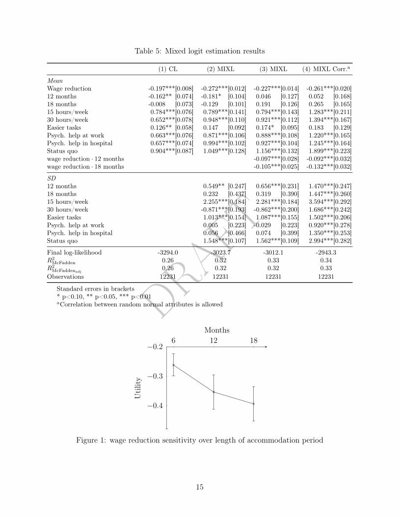
5.1 Main results

In table 11, the parameter estimates for the four different models are shown. Model (1)is a conditional logit (CL) model where homogeneous attribute preferences are assumed.In model (2), heterogeneity is allowed and thus standard deviations are estimated for therandom normal distributed attributes. A likelihood ratio test between model (1) and (2)results in a likelihood ratio value of 540.6 and a corresponding p-value p<0.001 (8 d.f.), andthus a significant improvement in the model fit is obtained when allowing for heterogeneity.This is also confirmed by examining the parameter adjusted Pseudo R2 which suggest aconsiderably greater explanatory power in the MIXL model compared to the CL model. Inmodel (2), the estimated standard deviations are significant, indicating that parameters doindeed vary in the sample. The mean coefficients are higher in model (2) than model (1) asthe variance of the error terms are normalized to set the scale of utility.11

Model (3) is an extension of model (2), with interactions between length of accommoda-tion period and wage reduction to examine whether the wage reduction sensitivity dependson the length of the accommodation period. It is seen that the included interaction termsare significantly negative and therefore that the survivors are less willing to experience awage reduction for a longer than a shorter period of time. A likelihood ratio test betweenmodel (2) and (3) again suggest a significant improvement in the model fit with a likelihoodratio value of 23.2 and a corresponding p-value at p<0.001 (2 d.f.).

In model (4), correlation between the random normal distributed parameters is allowed.Allowing for correlation involves estimation of 28 extra parameters as we estimate the lowertriangular covariance matrix between the random normal attributes. A likelihood ratio testbetween model (3) and (4) suggest a significant improvement with a likelihood ratio valueof 137.6 and a corresponding p-value of p<0.001 (28 d.f.). When examining the parameteradjusted Pseudo R2, the explanatory power is also slightly higher for model (4) than model(3). Thus, it is model (4) that the following willingness to pay estimates will be calculated

11Scale is inversely related to the error variance and cannot be separately identified. The solution istherefore to normalise for scale by normalising the variance of the error term. In the mixed logit modelparameter variance is treated as a separate component of the error, i.e. η′nxnit in Unit = β′xnit+η

′nxnit+εnit.

Hence εnit is net of parameter variance in the mixed logit model and will therefore be lower than in theconditional logit model. The parameters β are normalized such that εnit has the appropriate variance foran extreme value error. In the conditional logit model where Unit = β′xnit + εnit, β are normalized suchthat εnit has the variance of an extreme value deviate and the extreme value term will here incorporate anyvariance in the parameters (Revelt and K. Train 1998).

13

DRAFT

from and it is also model (4) we will extend with indicator interactions to examine sourcesof preference heterogeneity later. The higher log-likelihood value in model (4) reflects thatsignificant correlations between the attributes are present. Thus, when allowing for correla-tion, the parameter estimates for attributes which are highly correlated with other attributesincrease as more of the variance is captured. When examining the difference in parameterestimates from model (3) to model (4), it is not possible to determine what portion of thecorrelation is due to scale heterogeneity (smaller variance of the error term) and what portionis due to survivors preferring for instance both psychological help in the workplace and inthe hospital (higher total indirect utility). However, as we will calculate WtP estimates andas we will not make any parameter comparisons across samples (with potentially differentscales) the scale factor is irrelevant to examine further 12.

In figure 1, the wage reduction estimates over the length of accommodation period frommodel (4) are plotted, and it is seen that the sensitivity towards experiencing a wage re-duction to be accommodated increases over the three periods; 6, 12 and 18 months. Thisillustrates that the survivors are more willing to pay for the presented attributes for a shorterthan a longer period. With Wald tests for parameter equality, it is identified that the wagereduction sensitivity increases 35 pct. between 6 and 12 months, which is significant at a 95pct. confidence level, while there is no significant difference between 12 and 18 months.

12In calculation of WtP, the issue of scale heterogeneity disappears because of division, e.g. β∗1

β∗1

= λβ1

λβ2= β1

β2

14

DRAFT

Table 5: Mixed logit estimation results

(1) CL (2) MIXL (3) MIXL (4) MIXL Corr.a

MeanWage reduction -0.197***[0.008] -0.272***[0.012] -0.227***[0.014] -0.261***[0.020]12 months -0.162** [0.074] -0.181* [0.104] 0.046 [0.127] 0.052 [0.168]18 months -0.008 [0.073] -0.129 [0.101] 0.191 [0.126] 0.265 [0.165]15 hours/week 0.784***[0.076] 0.789***[0.141] 0.794***[0.143] 1.283***[0.211]30 hours/week 0.652***[0.078] 0.948***[0.110] 0.921***[0.112] 1.394***[0.167]Easier tasks 0.126** [0.058] 0.147 [0.092] 0.174* [0.095] 0.183 [0.129]Psych. help at work 0.663***[0.076] 0.871***[0.106] 0.888***[0.108] 1.220***[0.165]Psych. help in hospital 0.657***[0.074] 0.994***[0.102] 0.927***[0.104] 1.245***[0.164]Status quo 0.904***[0.087] 1.049***[0.128] 1.156***[0.132] 1.899***[0.223]wage reduction · 12 months -0.097***[0.028] -0.092***[0.032]wage reduction · 18 months -0.105***[0.025] -0.132***[0.032]

SD12 months 0.549** [0.247] 0.656***[0.231] 1.470***[0.247]18 months 0.232 [0.437] 0.319 [0.390] 1.447***[0.260]15 hours/week 2.255***[0.184] 2.281***[0.184] 3.594***[0.292]30 hours/week -0.871***[0.193] -0.862***[0.200] 1.686***[0.242]Easier tasks 1.013***[0.154] 1.087***[0.155] 1.502***[0.206]Psych. help at work 0.005 [0.223] -0.029 [0.223] 0.920***[0.278]Psych. help in hospital 0.056 [0.466] 0.074 [0.399] 1.350***[0.253]Status quo 1.548***[0.107] 1.562***[0.109] 2.994***[0.282]

Final log-likelihood -3294.0 -3023.7 -3012.1 -2943.3R2

McFadden 0.26 0.32 0.33 0.34R2

McFaddenadj0.26 0.32 0.32 0.33

Observations 12231 12231 12231 12231

Standard errors in brackets* p<0.10, ** p<0.05, *** p<0.01aCorrelation between random normal attributes is allowed

6 12 18

−0.4

−0.3

−0.2

Months

Utility

Figure 1: wage reduction sensitivity over length of accommodation period

15

DRAFT

In table 6, the WtP calculations are shown.13 It is seen that the survivors exhibit sig-nificant positive willingness to pay for working less hours and for receiving psychologicalhelp. Willingness to pay estimates for these attributes lie between 314 EUR and 359 EURmonthly for a period of 6 months. However, the survivors do not exhibit a significant WtPfor working on easier tasks. The significant WtP for the status quo option illustrates a strongpreference for the status quo option rather than being a useful WtP estimate. Wald testsfor parameter equality show that the willingness to pay for working 15 vs 30 hours are notsignificantly different from each other, and the same is true when comparing psychologicalhelp in the workplace vs the hospital. However, we will keep the attributes apart, as thestandard deviations around the mean estimates differ.

Table 6: WtP (EUR) based on model (4)

WtPa S.E. 95 pct. CF

6 months15 hours/week 330*** [57] 219 44130 hours/week 359*** [45] 270 447Easier tasks 47 [34] -19 113Psych. help at work 314*** [47] 222 406Psych. help in hospital 320*** [46] 230 410Status quo 488*** [67] 356 620

12 months15 hours/week 244*** [43] 159 32930 hours/week 265*** [36] 194 336Easier tasks 35 [25] -13 83Psych. help in workplace 232*** [36] 161 303Psych. help in hospital 236*** [36] 167 307Status quo 361*** [49] 265 458

18 months15 hours/week 219*** [38] 144 29430 hours/week 238*** [32] 176 300Easier tasks 31 [22] -12 75Psych. help in workplace 208*** [30] 150 267Psych. help in hospital 213*** [32] 150 275Status quo 324*** [43] 240 408

Standard errors in brackets* p<0.10, ** p<0.05, *** p<0.01WtP calculations are based on the coefficients from model (4) in table 11.First 6 months: WtP for working 30 hours relative to 37 hours/week 1.394

−(−0.261) ·5007.45 = 359 euro.

First 12 months: WtP for working 30 hours relative to 37 hours/week 1.394−(−0.261−0.092) ·

5007.45 = 265 euro.

13Over time the WtP are calculated by including the interaction between wage reduction and period:WtP 30 hours = − β̂30 hours

β̂p+β̂p*12 months· 5007.45

16

DRAFT

The estimated standard deviations provide important information about the distributionof preferences. In figure 2, the preference distributions are shown for receiving psychologi-cal help, working less hours and working on easier tasks. It is seen that the breast cancersurvivors agree more on their preferences for psychological help than working hours as theestimated standard deviations are larger for working less hours. When examining psycho-logical help, the two mean estimates for receiving psychological help in the workplace and inthe hospital are very close but we observe slightly more preference heterogeneity for psycho-logical help in the hospital. The distributions for working respectively 15 and 30 hours/weekrelative to 37 hours/week also yields interesting results. Here, it is seen that survivors agreemore on the valuation of working 30 hours/week than 15 hours/week. In particular, thestandard deviation for working 15 hours/week is remarkably large. This suggest that somesurvivors have a very high willingness to pay for working 15 hours/week while other sur-vivors experience a large disutility with working 15 hours/week compared to 37 hours/week.As we can observe heterogeneity among the breast cancer survivors through these signifi-cant standard deviations it is relevant to examine whether we can come closer at identifyingthe sources to the observed preference heterogeneity. This is done in the following by theinclusion of interaction terms between the random normal attributes and three importantindicators.

−10 −5 0 5 100

0.5

1

pdf

Psychologist in workplacePsychologist in hospital

−10 −5 0 5 100

0.5

1

pdf

15 hours/week30 hours/week

−10 −5 0 5 100

0.5

1

pdf

Easier tasks

Figure 2: Probability density functions, based on model (4)

17

DRAFT

5.2 Examining preference heterogeneity

Within the MIXL literature, preference heterogeneity has previously been accounted for inone of three ways; via random parameter estimates to reveal the presence of heterogeneitybut without explaining the source (Revelt and K. Train 1998); via the inclusion of interac-tion effects to systematically explain sources of heterogeneity (Small and Lam 2001); via acombination of both interaction effects and random parameters (Hensher and Greene 2003).In this paper, we apply the last of the three approaches, as we both allow the main attributesto be random normal distributed and as we include indicator interactions to examine ob-servable sources of preference heterogeneity. The interaction terms are kept fixed as theopposite would require a lot of variation within the indicator groups and as random normaldistributed interaction terms also increase the computational burden in Stata.

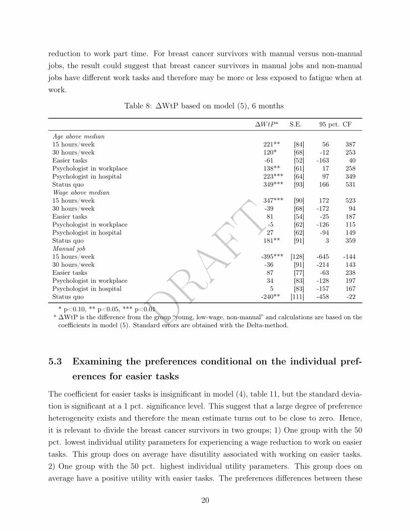
In the following, the reference case is young, low wage breast cancer survivors workingin non-manual jobs are compared with each of the three comparison groups; 1) age abovethe sample median, 2) wage above the sample median and 3) having a manual- or servicejob. The MIXL and WtP results14 are shown in table 7, while ∆WtP is shown in table8. The results in table 8 show that preference heterogeneity in age is elicited, where breastcancer survivors with ages above the median age in the sample on average are more willingto experience a wage reduction to receive psychological help and to work less hours thansurvivors with ages below the median age (54 years). This could suggest that older breastcancer survivors have different needs than younger survivors due to specific age-dependentcomplications such as slower recovery.

14 Mean WtP for working 30 hours/week compared to 37 hours/week for the reference group of young,low wage breast cancer survivors working in non-manual jobs can be calculated by the simple measure

WtP 30hours =β̂30hours

−β̂p· 500

7.45(9)

When examining preference differences across wage, this will be compared with mean WtP for young, highwage breast cancer survivors working in non-manual jobs

WtP 30hours·wage =β̂30hours + β̂30hours·wage

−(β̂p + β̂p·wage)· 500

7.45(10)

The mean difference in WtP between the reference group and the comparison group can then be calculatedas

∆WtP = WtP 30hours·wage −WtP 30hours (11)

which is interpreted as the extra WtP high wage breast cancer survivors exhibit compared to low wage breastcancer survivors to obtain a working week of 30 hours compared to 37 hours/week, all else equal. Standarderrors for ∆WtP are as for the WtP estimates also estimated with the Delta Method and are calculateddirectly from the MIXL coefficients to avoid approximate standard errors two times.

18

DRAFT

Table 7: Mixed logit estimation results, model (5), and WtP (EUR)

Reference groupa Age above median wage above median Manual job

Meanwage reduction -0.328*** [0.027] 0.057** [0.023] 0.049** [0.024] 0.064** [0.025]12 months -0.239 [0.226] 0.125 [0.230] 0.368 [0.248] -0.199 [0.289]18 months -0.114 [0.241] 0.122 [0.243] 0.669*** [0.258] -0.640** [0.299]15 hours/week 0.461 [0.352] 0.813** [0.370] 1.374*** [0.391] -1.642*** [0.465]30 hours/week 1.537*** [0.261] 0.217 [0.274] -0.391 [0.288] -0.441 [0.348]Easier tasks 0.110 [0.213] -0.267 [0.230] 0.320 [0.239] 0.321 [0.297]Psychologist in workplace 1.095*** [0.246] 0.364 [0.254] -0.187 [0.270] -0.079 [0.316]Psychologist in hospital 0.941*** [0.249] 0.735*** [0.258] -0.028 [0.269] -0.163 [0.319]Status quo 1.088*** [0.330] 1.215*** [0.352] 0.589 [0.367] -1.158*** [0.435]Wage reduction · 12 months -0.096*** [0.031]Wage reduction · 18 months -0.125*** [0.030]SD12 months 0.453* [0.269]18 months 0.947*** [0.249]15 hours/week 3.317*** [0.272]30 hours/week 1.541*** [0.239]Easier tasks 1.444*** [0.198]Psychologist in workplace 0.839*** [0.259]Psychologist in hospital 1.311*** [0.260]Status quo 2.665*** [0.276]

Final log-likelihood -2904.2R2

McFadden 0.35R2

McFaddenadj0.34

Observations 12231

Reference group Age above median Wage above median Manual job

WtP, 6 months (EUR)15 hours/week 94 [72] 316*** [82] 442*** [86] -300** [151]30 hours/week 315*** [56] 435*** [66] 276*** [67] 279** [109]Easier tasks 23 [44] -39 [49] 104** [52] 110 [91]Psychologist in workplace 224*** [52] 362*** [63] 220 *** [62] 258** [101]Psychologist in hospital 192*** [53] 415*** [65] 220*** [61] 198** [101]Status quo 223*** [72] 571*** [95] 404*** [91] -18 [133]

Standard errors in brackets* p<0.10, ** p<0.05, *** p<0.01aCorrelation between random normal attributes is allowed

For the 15 hours/week attribute, two sources of heterogeneity have been elicited. Breastcancer survivors with a wage above the median wage have a significantly higher willingnessto pay for working 15 hours/week than survivors with a wage below the median (46,760EUR). Further, breast cancer survivors working in manual jobs have a significantly lowerwillingness to pay for working 15 hours/week than survivors working in non-manual jobs.In regards to the higher willingness to pay among high wage survivors, the result is likely toillustrate that high wage survivors have the financial possibility of experiencing a large wage

19

DRAFT

reduction to work part time. For breast cancer survivors with manual versus non-manualjobs, the result could suggest that breast cancer survivors in manual jobs and non-manualjobs have different work tasks and therefore may be more or less exposed to fatigue when atwork.

Table 8: ∆WtP based on model (5), 6 months

∆WtP a S.E. 95 pct. CF

Age above median15 hours/week 221** [84] 56 38730 hours/week 120* [68] -12 253Easier tasks -61 [52] -163 40Psychologist in workplace 138** [61] 17 258Psychologist in hospital 223*** [64] 97 349Status quo 349*** [93] 166 531Wage above median15 hours/week 347*** [90] 172 52330 hours/week -39 [68] -172 94Easier tasks 81 [54] -25 187Psychologist in workplace -5 [62] -126 115Psychologist in hospital 27 [62] -94 149Status quo 181** [91] 3 359Manual job15 hours/week -395*** [128] -645 -14430 hours/week -36 [91] -214 143Easier tasks 87 [77] -63 238Psychologist in workplace 34 [83] -128 197Psychologist in hospital 5 [83] -157 167Status quo -240** [111] -458 -22

* p<0.10, ** p<0.05, *** p<0.01a ∆WtP is the difference from the group “young, low-wage, non-manual” and calculations are based on thecoefficients in model (5). Standard errors are obtained with the Delta-method.

5.3 Examining the preferences conditional on the individual pref-

erences for easier tasks

The coefficient for easier tasks is insignificant in model (4), table 11, but the standard devia-tion is significant at a 1 pct. significance level. This suggest that a large degree of preferenceheterogeneity exists and therefore the mean estimate turns out to be close to zero. Hence,it is relevant to divide the breast cancer survivors in two groups; 1) One group with the 50pct. lowest individual utility parameters for experiencing a wage reduction to work on easiertasks. This group does on average have disutility associated with working on easier tasks.2) One group with the 50 pct. highest individual utility parameters. This group does onaverage have a positive utility with easier tasks. The preferences differences between these

20

DRAFT

two groups will be examined in the following.

First, we compare descriptive statistics across the two groups. From table 9 it is seen thatthe group which prefer easier tasks and the group which does not are similar on age, job type,educational level and ability to work during treatment. They differ on wage level where thesurvivors who have disutility associated with easier tasks on average earn 4000 EUR moreannually. They also differ slightly on self-perceived ability to work during treatment, wherethe survivors who on average would like to work on easier tasks rate their ability to workslightly lower. This could explain why this is also the group preferring easier tasks.

Table 9: Descriptive statistics across individual preferences for easier task

Disutility for easier tasks Positive utility for easier tasks t-test

Age 53.14 [6.86] 53.55 [7.02]Annual wage (1000 EUR) 48.76 [18.92] 44.76 [18.59] ***Manual job (0/1) 0.19 [0.39] 0.21 [0.41]Education 2.46 [0.91] 2.43 [0.84]Ability to work during treatment 2.46 [2.55] 2.27 [2.69]Ability to work 1 year after end oftreatment

7.36 [2.51] 6.61 [2.72] ***

Observations 6108 6123Respondents 354 350

* p<0.10, ** p<0.05, *** p<0.01Standard deviations in bracketsSelf-perceived ability to work is measured on a scale from 0-10.Education is measured on a scale from 1-4

In table 10 the WtP results are presented while the utility parameters are left to the ap-pendix. The results show that the group with disutility for easier tasks on average wouldprefer a work week on 30 hours/week and psychological help in the hospital. The group whowould like to work on easier tasks prefer to work 15 hours/week and to receive psychologicalhelp at work. From the estimated utility parameters shown in the appendix, it is seen thatthe group who dislikes easier tasks have strong negative preferences for being accommodatedin 18 months compared to 6 months while the other group have strong preferences towardsan accommodation period of 18 months compared to 6 months. From figure 3, it is furtherseen that the group which do not want to be accommodated with easier tasks are not wagesensitive to the length of the accommodation period. The breast cancer survivors who arewilling to experience a wage reduction to work on easier tasks have a significantly higherwillingness to pay in the first six months than in 12 and 18 months respectively. Thus, thegroup which prefer easier tasks prefer a long period over a short period but they are sensitive

21

DRAFT

towards experiencing a wage reduction in a long period.

Table 10: WtP based on model (6) and (7) (EUR)

Disutility for easier tasks Positive utility for easier tasks t-test

6 months15 hours/week 346*** [90] 380*** [75]30 hours/week 609*** [83] 207*** [52] ***Easier tasks -478*** [50] 709*** [75] ***Psych. help at work 255*** [61] 438*** [61] **Psych. help in hospital 462*** [67] 244*** [58] **Status quo 471*** [97] 710*** [116]12 months15 hours/week 277*** [76] 265*** [57]30 hours/week 489*** [79] 144*** [37] ***Easier tasks -383*** [55] 494*** [59] ***Psych. help at work 205*** [54] 305*** [49]Psych. help in hospital 370*** [65] 170*** [44] **Status quo 378*** [82] 495*** [80]18 months15 hours/week 310*** [88] 226*** [45]30 hours/week 546*** [98] 123*** [32] ***Easier tasks -428*** [66] 421*** [42] ***Psych. help at work 228*** [61] 260*** [35]Psych. help in hospital 414*** [83] 145*** [35] ***Status quo 422*** [98] 422*** [62]

Observations 6108 6123

* p<0.10, ** p<0.05, *** p<0.01Standard errors in brackets

6 12 18

−0.6

−0.4

−0.2

0

Months

Utility

Disutility for easier tasksPositive utility for easier tasks

Figure 3: Wage reduction sensitivity over time

22

DRAFT

6 Discussion [To be continued]

In Denmark a consultation with a psychologist costs approximately 55 EUR if you get amedical referral through your doctor and approximately 150 EUR without. Cancer patientsin Denmark have the right to receive a medical referral up to 12 months after diagnosiswhere the maximum number of consultations with reimbursement is 12. If patients receive1 to 4 consultations a month the first six months after treatment, this will on average resultin individual expenses in the range 55 - 410 EUR for the patient monthly. We estimated awillingness to pay for psychological help on 314 EUR monthly if received in the work placeand 320 EUR if received in the hospital the first 6 months.

In our sample the average annual wage is 46,700 suggesting an average monthly wage at3,891 EUR. Hence, a reduction in working hours of 7 hours a week will approximately cost737 EUR monthly. As the breast cancer survivors were willing to pay on average 359 EURfor working 30 hours weekly instead of 37 they are not willing to pay as much as the actualcost for the employer, but they are willing to take on approximately half of the cost.

23

DRAFT

7 Conclusion

We have estimated breast cancer survivors’ willingness to pay for accommodating attributes.On average psychological help (in the workplace or the hospital) and a shorter working week(15 or 30 hours/week) is highly valued with willingness to pay estimates ranging from 314to 359 EUR monthly the first six months after returning to work after treatment. Thesurvivors agree highly on the valuation of psychological help while they a more dispersed intheir preferences for working hours. When examining the sources of preference heterogeneityin the valuation of working hours, it is seen that breast cancer survivors with ages above themedian age are relatively more willing to pay for receiving psychological help and workingless hours than survivors with ages below the median age suggesting different needs forolder breast cancer survivors. Two other sources of preference heterogeneity have beenelicited for the 15 hours/week attribute. Breast cancer survivors with an income abovethe median income have a significantly higher willingness to pay for working 15 hours/weekthan survivors with an income below the median. Breast cancer survivors working in manual-or service jobs have a significantly lower willingness to pay for working 15 hours/week thansurvivors working in non-manual jobs. Where the first source suggest the financial possibilityof experiencing a large wage reduction to work part time when having a high income, thelatter could suggest that breast cancer survivors in manual jobs and non-manual jobs havedifferent work tasks and therefore may be more or less exposed to fatigue when at work.

24

DRAFT

References

Barton, D et al. (2010). “Abstract P2-14-10: Self Reported Cognitive Function in BreastCancer Survivors: A 12 Month Longitudinal Descriptive Study”. In: Cancer Research70.24 Supplement, P2-14-10–P2-14-10. issn: 0008-5472.

Bouknight, Reynard R, Cathy J Bradley, and Zhehui Luo (2006). “Correlates of return towork for breast cancer survivors”. In: Journal of Clinical Oncology 24.3, pp. 345–353.

Bower, Julienne E (2008). “Behavioral symptoms in patients with breast cancer and sur-vivors”. In: Journal of clinical oncology : official journal of the American Society of Clin-ical Oncology 26.5. issn: 1527-7755.

Caldon, Lisa J.M. et al. (2007). “What influences clinicians operative preferences for womenwith breast cancer? An application of the discrete choice experiment”. In: European Jour-nal of Cancer 43.11, pp. 1662–1669.

Calvio L., Lisseth et al. (2010). “Measures of Cognitive Function and Work in Occupation-ally Active Breast Cancer Survivors”. In: Journal of Occupational and EnvironmentalMedicine 52.2, pp. 219–227. issn: 1076-2752.

Cancer Research UK (2018). Cancer Statistics - Incidence. url: http://www.cancerresearchuk.org/health-professional/cancer-statistics/incidence.

Fujimori, Maiko et al. (2006). “Preferences of cancer patients regarding the disclosure of badnews”. In: Psycho-Oncology 16.6, pp. 573–581.

Hansen, Jennifer A et al. (2008). “Breast cancer survivors at work”. In: Journal of Occupa-tional and Environmental Medicine 50.7, pp. 777–784.

Heinesen, Eskil et al. (2016). “Return to work after cancer and pre-cancer job dissatisfaction”.In: The Rockwool Foundation Research Unit 108.

Hensher, D. A and W. H. Greene (2003). “The Mixed Logit Model: The State of Practice”.In: Transportation 30.2, pp. 133–176.

Hole, Arne Risa and Julie Riise Kolstad (2012). “Chapter: 3 Mixed logit estimation og will-ingness to pay distributions: a comparison of models in preference and WTP space usingdata from a health-related choice experiment”. In: Empirical Economics 42.1, pp. 76–84.

Mcfadden, Daniel (1973). “Conditional logit analysis of qualitative choice behavior”. In: Fron-tiers in Econometrics. Ed. by P. Zarembka. New York: Academic Press. Chap. 4, pp. 105–142.

Mehnert, Anja (2011). “Employment and work-related issues in cancer survivors”. In: CriticalReviews in Oncology / Hematology 77.2, pp. 109–130.

Neumark, David et al. (2015). “Work Continuation while Treated for Breast Cancer: TheRole of Workplace Accommodations”. In: ILR Review 68.4, pp. 916–954.

25

DRAFT

Parry, Carla et al. (2011). “Cancer survivors: a booming population”. In: Cancer Epidemiologyand Prevention Biomarkers 20.10, pp. 1996–2005.

Revelt, David and Kenneth Train (1998). “Mixed logit with repeated choices: households’choices of appliance efficiency level”. In: University of California, Berkeley, pp. 647–657.

Small, Kenneth A. (2012). “Valuation of travel time”. In: Economics of Transportation 1.1-2,pp. 2–14.

Small, Kenneth A. and T. C. Lam (2001). “The value of time and reliability: Measurementfrom a value pricing experiment”. In: Transportation Research Part E 37.2-3, pp. 231–251.

Tasmuth, T., Kvon Smitten, and E. Kalso (1996). “PP-2-15 Pain and other symptoms duringthe first year after surgery for breast cancer”. eng. In: European Journal of Cancer 32.issn: 09598049.

Tessier, Philippe, Myriam Blanchin, and Veronique Sebille (2017). “Does the relationshipbetween health-related quality of life and subjective well-being change over time? Anexploratory study among breast cancer patients”. In: Social Science & Medicine 174,pp. 96–103.

The Danish Cancer Society (2017). Working after Cancer. url: https://www.cancer.dk/hjaelp-viden/hvis-du-har-kraeft/arbejde/arbejde-efter-kraeft/ (visited on05/26/2017).

Train, Kenneth E. (2003). Discrete Choice Methods with Simulation. 1st ed. CambridgeUniversity Press.

World Health Organization - International Agency for Research on Cancer (2012). EstimatedCancer Incidence, Mortality and Prevalence Worldwide in 2012. url: http://globocan.iarc.fr/Pages/fact_sheets_cancer.aspx.

Zhao, Yong, Kara Kockelman, and Anders Karlstrom (2012). “Welfare calculations in discretechoice settings: The role of error term correlation”. In: Transport Policy 19.1, pp. 76–84.

26

DRAFT

Appendix A

Table 11: Mixed logit estimation results, model (6) and (7)

(6) MIXL (7) MIXL

MeanWage reduction -0.297***[0.030] -0.275***[0.025]12 months 0.260 [0.302] -0.248 [0.212]18 months 1.046***[0.282] -0.955***[0.267]15 hours/week 1.682***[0.327] 1.415***[0.370]30 hours/week 0.916***[0.235] 2.493***[0.335]Easier tasks 3.141***[0.291] -1.955***[0.191]Psych. help at work 1.941***[0.252] 1.043***[0.253]Psych. help in hospital 1.081***[0.247] 1.888***[0.272]Status quo 3.146***[0.437] 1.929***[0.384]Wage reduction · 12 months -0.129***[0.050] -0.068 [0.046]Wage reduction · 18 months -0.203***[0.043] -0.032 [0.047]SD12 months 1.471***[0.504] 1.384***[0.362]18 months 1.861***[0.360] 1.570***[0.319]15 hours/week 4.283***[0.459] 3.590***[0.505]30 hours/week 1.422***[0.448] 2.182***[0.423]Easier tasks 1.518***[0.279] 0.350 [0.236]Psych. help at work 1.311***[0.350] 1.105***[0.380]Psych. help in hospital 1.476***[0.351] 1.609***[0.398]Status quo 4.963***[0.498] 2.724***[0.460]

Final log-likelihood -1294.6 -1289.9R2

McFadden 0.42 0.42R2

McFaddenadj0.39 0.39

Observations 6123 6108

Standard errors in brackets* p<0.10, ** p<0.05, *** p<0.01aCorrelation between random normal attributes is allowed

27