Pull Manufacturing System Design for Rough Mill Systems: A Case Study

Garrett Todd Norman

Thesis submitted to the faculty of Virginia Polytechnic Institute and State University in partial fulfillment of the requirements for the degree of

Master of Science

In Wood Science and Forest Products

Dr. D. Earl Kline, Chair

Dr. Brian H. Bond

Dr. Robert L. Smith

May 5, 2008 Blacksburg, VA

Keywords: Rough Mill, Value Stream, Pull Production, Supermarket

Pull Manufacturing System Design for Rough Mill Systems: A Case Study

Garrett Todd Norman

ABSTRACT Domestic secondary wood products manufacturers are losing their competitive

edge in the global economy. Foreign competition is steadily gaining market-share due to

decreased labor costs. While domestic operations can not compete with labor costs

available to foreign manufacturers, they may be able to remain competitive through

product lead time reduction and on-time delivery to the final customer. Pull based

manufacturing is one technique to reduce lead time increase on-time delivery.

Value stream mapping was used in this project to evaluate a furniture rough mill

located in Virginia to assess the current state, as well as develop 2 future state value

streams. The current state evaluation found the system to be yield driven and production

was based on a forecast. The lead time for internal nightstand components in the current

state was found to be 15.1 hours. Using pull production and supermarket methodology in

proposed future states, it was found that the lead time could be reduced to 7.5 hours.

Lead times could be reduced by eliminating yield increasing non-value added activities

currently in place which not only increase lead time, but also manufacturing waste as

defined by lean manufacturing concepts. A cost analysis found that the labor and

overhead costs associated with yield increasing activities in the current state outweighed

the costs of a decreased yield measurement in the future state.

While this project was limited to one rough mill and one product family of a

lesser valued wood species it represents what is possible for assisting secondary

manufacturers to remain competitive. The once successful traditional yield driven rough

iii

mill does not guarantee internal customer satisfaction and in this project is not cost

effective. Future research should focus on the implications of the furniture rough mill’s

inability to meet downstream demand to internal customers.

iv

Acknowledgements

I would like to thank the following people for their support of this research project. My most sincere thanks and appreciation to: Dr. D. Earl Kline who served as my advisor and provided me with guidance and support throughout this research project. Dr. Brian H. Bond and Dr. Robert L. Smith for serving on my committee and providing valuable input. Kevin Wampler, Andy Poore, Eric Jones, Larry Hagwood, J.L. Fackler Jr. and Marco Taylor for the endless hours spent educating me on how a rough mill and furniture plant operate. This project would be non-existent without their support. My fellow graduate students of the Wood Science department, especially: Alex Hagedorn, Tim Stiess, Omar Espinoza, Braden White, Jim Bisha, Brian Perkins, and Patrick Rappold for always providing support and entertainment outlet. Dan Cumbo for his words of wisdom and sparking my interest in continuous improvement. Elaine for all the love and words of encouragement that remained constant throughout the entirety of this project. My special thanks go to my parents, Gary and Kimbra Norman for everything I am today. Words can not describe their everlasting support and love.

v

Pull Manufacturing System Design for Rough Mill Systems

Table of Contents

LIST OF TABLES AND FIGURES.............................................................................. VIII

1 PROBLEM STATEMENT AND RESEARCH OBJECTIVES................................. 1

1.1 PROBLEM STATEMENT ......................................................................................... 1 1.2 RESEARCH OBJECTIVES ....................................................................................... 2 1.3 APPROACH ........................................................................................................... 3 1.4 LIMITATIONS........................................................................................................ 4

2 LITERATURE REVIEW ........................................................................................... 5

2.1 WOODEN FURNITURE MANUFACTURING TRENDS IN THE UNITED STATES........... 5 2.2 WOODEN FURNITURE MANUFACTURING PROCESSES........................................... 6 2.3 THE ROUGH MILL ................................................................................................ 9

2.3.1 The Rough Mill Defined............................................................................. 9 2.3.2 Rough Mill Costs ...................................................................................... 11 2.3.3 Performance Measures.............................................................................. 12 2.3.4 Yield.......................................................................................................... 13 2.3.5 Rough Mill Yield Simulation.................................................................... 13 2.3.6 Demand ..................................................................................................... 14 2.3.7 Flexibility.................................................................................................. 15 2.3.8 Over-Run (Overages)................................................................................ 15 2.3.9 Production Scheduling.............................................................................. 16

2.4 PRODUCTION CONTROL SYSTEMS ...................................................................... 17 2.4.1 Push Systems ............................................................................................ 18 2.4.2 Pull manufacturing / Just-in-time.............................................................. 19 2.4.3 Inventory Control...................................................................................... 21

2.5 VALUE STREAM MAPPING ................................................................................. 23

3 ROUGH MILL CURRENT STATE EVALUATION ............................................. 26

3.1 INTRODUCTION .................................................................................................. 26 3.2 METHODS .......................................................................................................... 26 3.3 MANUFACTURER PROFILE ................................................................................. 29 3.4 NIGHTSTANDS.................................................................................................... 30 3.5 PRODUCTION SCHEDULING ................................................................................ 32 3.6 CURRENT STATE ROUGH MILL VALUE STREAM ................................................ 33 3.7 LUMBER YARD .................................................................................................. 39 3.8 THE ROUGH MILL .............................................................................................. 40

3.8.1 Lumber Input ............................................................................................ 41 3.8.2 Rough Planer/Gang-Rip/Chop Operations ............................................... 42 3.8.3 Edge Gluing Operation ............................................................................. 47 3.8.4 Multi-Rip Operation.................................................................................. 48 3.8.5 Moulders ................................................................................................... 48

vi

3.9 YIELD ................................................................................................................ 50 3.10 WORK TIME ....................................................................................................... 51 3.11 ON-TIME DELIVERY........................................................................................... 52 3.12 CURRENT STATE IMPROVEMENT OPPORTUNITIES .............................................. 54

3.12.1 Overproduction ......................................................................................... 54 3.12.2 Unnecessary Inventory.............................................................................. 55 3.12.3 Waiting...................................................................................................... 55 3.12.4 Inappropriate Processing........................................................................... 56 3.12.5 Defects ...................................................................................................... 57 3.12.6 Transportation ........................................................................................... 58 3.12.7 Motion....................................................................................................... 59 3.12.8 Opportunities Summary ............................................................................ 60

4 ROUGH MILL FUTURE STATE EVALUATION................................................. 61

4.1 INTRODUCTION .................................................................................................. 61 4.2 METHODS .......................................................................................................... 61 4.3 FUTURE STATE VALUE STREAM MAPPING......................................................... 62

4.3.1 Future State Value Stream Map #1........................................................... 65 4.3.2 Future State Value Stream Map #2........................................................... 67

4.4 SUPERMARKET ................................................................................................... 68 4.4.1 A, B, C Analysis ........................................................................................ 69 4.4.2 Supermarket Inventory Levels.................................................................. 71

4.5 YIELD SIMULATION ........................................................................................... 74 4.5.1 Current State ROMI-3 Settings................................................................. 74 4.5.2 Future State ROMI-3 Settings .................................................................. 77 4.5.3 Lumber Input ............................................................................................ 77 4.5.4 Cutting Bills .............................................................................................. 78 4.5.5 Panel Production ....................................................................................... 81 4.5.6 Methods..................................................................................................... 81

4.6 LEAD TIME......................................................................................................... 85 4.7 ON-TIME DELIVERY........................................................................................... 85 4.8 IMPROVEMENT OPPORTUNITIES ......................................................................... 86

4.8.1 Overproduction ......................................................................................... 86 4.8.2 Unnecessary Inventory.............................................................................. 87 4.8.3 Waiting...................................................................................................... 87 4.8.4 Inappropriate Processing........................................................................... 87 4.8.5 Defects ...................................................................................................... 88 4.8.6 Transportation ........................................................................................... 89 4.8.7 Motion....................................................................................................... 89

5 VALUE STREAM EVALUATIONS FOR COST EFFECTIVENESS................... 90

5.1 METHODS .......................................................................................................... 91 5.2 CURRENT STATE VALUE STREAM ...................................................................... 91

5.2.1 Lumber, Processing and Total Costs ........................................................ 92 5.3 FUTURE STATE VALUE STREAM #1.................................................................... 94 5.4 FUTURE STATE VALUE STREAM #2.................................................................... 95

5.4.1 Lumber, Processing and Total Costs ........................................................ 95

vii

5.5 BREAK EVEN POINT ........................................................................................... 98 5.6 TOTAL COST SAVING POTENTIAL ...................................................................... 99

6 CONCLUSIONS..................................................................................................... 101

6.1 RESEARCH OBJECTIVES FINDINGS ................................................................... 102 6.1.1 Objective 1 .............................................................................................. 103 6.1.2 Objective 2 .............................................................................................. 103 6.1.3 Objective 3 .............................................................................................. 104

6.2 FUTURE RESEARCH AND LIMITATIONS ............................................................ 105

REFERENCES ............................................................................................................... 107

APPENDIX..................................................................................................................... 112

viii

List of Tables and Figures List of Tables: Table 2-1 Options for finished goods versus make-to-order (Smalley 2004) .................. 22 Table 2-2 Finished goods calculation ............................................................................... 23 Table 3-1 Collection methods for determining current state value stream and waste ...... 28 Table 3-2 Rough mill processing sequences..................................................................... 34 Table 3-3 Internal nightstand component order (BBR#1) ................................................ 35 Table 3-4 Current state value stream map breakdown...................................................... 39 Table 3-5 Rough mill labor per machine per shift ............................................................ 39 Table 3-6 Standard 4/4’’ 2-C Poplar Arbor used by study mill........................................ 44 Table 3-7 Moulder assignments........................................................................................ 49 Table 3-8 Available Work Time in Rough Mill ............................................................... 51 Table 3-9 Overages example according to MRP .............................................................. 57 Table 4-1 Differing SKU's with identical physical characteristics................................... 69 Table 4-2 Part grouping based on Table 4-1..................................................................... 70 Table 4-3 Finished goods inventory level calculation ...................................................... 71 Table 4-4 Finished good inventory level example............................................................ 72 Table 4-5 “A” Supermarket finished goods inventory levels ........................................... 73 Table 4-6 “B” Supermarket finished good inventory levels ............................................. 73 Table 4-7 Rip-saw inputs .................................................................................................. 75 Table 4-8 Chop-saw Inputs............................................................................................... 75 Table 4-9 Mill control....................................................................................................... 76 Table 4-10 Salvage Parts Inputs ....................................................................................... 76 Table 4-11 Part Grade parameters .................................................................................... 76 Table 4-12 BF Grade Distribution ................................................................................... 78 Table 4-13 Board Length Distribution.............................................................................. 78 Table 4-14 Example of part length adjustment................................................................. 79 Table 4-15 Internal nightstand components in Bill #1 and Bill #2................................... 80 Table 4-16 T-test results and statistics of actual and simulated yield models .................. 83 Table 5-1 Current State Value Stream Lumber Costs for order BBR#1 .......................... 92 Table 5-2 Rough Planer/Gang-Rip/Chop-saw costs ......................................................... 92 Table 5-3 High-frequency gluing operation processing costs .......................................... 93 Table 5-4 Multi-Rip operating costs ................................................................................. 93 Table 5-5 Moulder costs ................................................................................................... 93 Table 5-6 Total Cost of Current State value stream to produce order BBR #1 ................ 94 Table 5-7 Future State Value Stream Map #2 Lumber Costs........................................... 96 Table 5-8 Rough Planer/Gang-Rip/Chop-saw Costs ........................................................ 96 Table 5-9 Total Cost of Future State Value Stream #2 to produce order BBR #1 ........... 96 Table 5-10 Yield Adjustments to Determine Break Even Point....................................... 98 Table 5-11 Yearly costs to produce internal nightstand components ............................... 99

ix

List of Figures: Figure 1-1 Approach ........................................................................................................... 3 Figure 2-1 Wooden furniture imported from China from 1996 to 2006 (U.S.D.C 2007). . 5 Figure 2-2 Manufacturing steps of wooden furniture ......................................................... 6 Figure 2-3 Continuous edge glue process example (Willard 1970) ................................. 10 Figure 2-4 Where dollars go in rough mill manufacturing (Mitchell et. al 2005) ............ 12 Figure 2-5 An example of a supermarket pull system (Rother and Shook 2003)............. 20 Figure 3-1 Products sold by manufacturer as a % of sales volume in 2006 ..................... 30 Figure 3-2 Top Blind Rail................................................................................................. 31 Figure 3-3 Top Back Rail ................................................................................................. 31 Figure 3-4 Production scheduling..................................................................................... 32 Figure 3-5 Current State Value Stream Map .................................................................... 36 Figure 3-6 Yield Results from 15 4/4’’ 2-C poplar cuttings............................................. 50 Figure 3-7 Timeline of on-time percentages based on the “off-schedule” ...................... 53 Figure 4-1 Finished goods inventory example (Rother and Shook 2003) ........................ 64 Figure 4-2 Rough mill Future State Value Stream Map #1 .............................................. 66 Figure 4-3 Rough mill Future State Value Stream Map #2 .............................................. 68 Figure 5-1 Furniture manufacturing costs (provided by study site) ................................. 90 Figure 5-2 Total Cost of Current State Value Stream to produce order BBR #1 ............. 94 Figure 5-3 Total Cost of Future State Value Stream #2 to produce order BBR #1.......... 97 Figure 5-4 Total Cost breakdown ..................................................................................... 98 Figure 5-5 Break even yield measure ............................................................................... 99 Figure 5-6 All Internal Components Yearly Costs ......................................................... 100

1

1 Problem Statement and Research Objectives

1.1 Problem Statement

Traditional secondary wood products manufacturers are losing their

competitiveness in the new global economy. The industry is responding by developing

capacity and expertise in dealing with outsourcing to lower cost regions. Foreign

manufacturers, specifically those in China and other Asian countries, have increased their

share of the United States wood household furniture market to the point that they provide

more than half of the furniture demanded in the United States (Bumgardner et al. 2004).

Secondary wood products manufacturing research has focused on locally

optimizing high cost work centers such as drying and rough mill yield primarily because

of the high percentage of total material product cost incurred in such operations. While

simulation and optimization in previous research successfully helped maximize industry

yield, it has been shown high yield emphasis results in large batch sizes, excessive re-

work, high work-in-progress levels and increased production lead times (Willard 1970;

Thomas and Buehlmann 2007). Increased lead times prevent the rough mill from

meeting demand changes downstream effectively.

Schuler et al. (2002) noted that companies must prepare for a shift from the old

world of mass production to the new business world where variety and customization of

products and services are the norm. This shift can be seen in kitchen and bath companies

as this segment of the industry has not lost significant business due to imports by quickly

and more precisely responding to local customer need (Ray et al. 2006).

As seen in kitchen and bath companies, future competitiveness depends on system

optimization by focusing on what will make secondary manufacturing more effective at

2

meeting customer demand. Traditional yield based operations do not guarantee part

requirements will be met efficiently to meet real customer demand in a timely manner.

This study will focus on better connecting the lumber processing system (rough mill) to

downstream customer processes (machining and assembly), as a first step to optimizing

the entire system.

1.2 Research Objectives

The goal of this research was to study the overall cost effectiveness of achieving

yield but not meeting actual demand in the rough mill. This research provides a method

for furniture rough mills to become more responsive to downstream customer demand.

The project involved a case study of a large sized furniture manufacturer’s rough mill

located in Virginia. It was hypothesized that many non-value added processes exist that

increase production cost and reduce rough mill effectiveness at meeting demand. Many

of these non-value added processes deal with overproduction, inappropriate processing,

part transportation, and expediting parts in immediate demand. Techniques such as pull

systems and supermarkets are discussed as a strategy to balance between cutting yield vs.

precise yield of demanded parts. The specific research objectives were:

1) To perform a current state value stream evaluation of the rough mill

manufacturing system.

2) To design an improved rough mill future state value stream that is responsive to

downstream demand using pull system methodologies.

3) To demonstrate the cost effectiveness of the future state value stream using a

furniture manufacturing case study.

3

1.3 Approach

This research focused on rough mill operations, particularly, how yield influences

operations (Figure 1-1). It was hypothesized that many hidden costs are added in the

yield optimization system. While these optimization systems were effective at one time,

they may not be as effective today or not for certain product value streams. This study

develops and demonstrates a methodology to understand the true cost effectiveness of the

entire system.

While this study focuses on how yield influences operations, it is important to note

that the objective of downstream furniture operations is to minimize unit cost of

machining and assembly as well as the order backlog handling system. The downstream

furniture operations objective adds cost that can be more significant than the rough’s mill

focus on yield. This study’s methodology can be applied to future research to understand

how downstream cost effectiveness adds into the system.

Figure 1-1 Approach

4

The objectives of each operation shown in Figure 1-1 are to minimize local costs,

often times this approach does not accurately meet true demand needs on-time. In rough

mill operations, maximizing yield is the way to minimize lumber costs therefore yield

optimization systems are developed. This further removes the focus away from demand,

plus adds system costs in non-value added activities that may negate yield benefits.

Furniture assembly operations require the system to deal with order backlogs; this adds

costs that can negate yield benefits. The rough mill schedule needs to be altered to make

up for critical backlogs, this alteration further increases costs.

1.4 Limitations

This project was limited to the boundary of the rough mill of a furniture

manufacturer. While this project may prove to be beneficial for the rough mill, the real

opportunity is beyond the rough mill. The cost of not meeting demand in the studied

operation was outside the scope of this project as all costs associated with backlog and

reschedules were unavailable. However, it is an area that future research should focus on

and should not be limited to just the rough mill.

The value streams were limited to internal nightstand components. This was done

because the system is too complex to take on all value streams. The methods used focus

on all issues in-depth for one component; this approach is also applicable for other

component value streams. Similar opportunities are hypothesized and require additional

future state development. Yield simulation was used in this project and can only be

assumed to represent the study rough mill. While simulation is a working research tool,

it cannot simulate exactly what a rough mill does.

5

2 Literature Review

2.1 Wooden Furniture Manufacturing Trends in the United States

A recent survey found that 61% of large home furnishings manufacturing

executives agreed with the statement that by the end of the decade, little will remain of

domestic wood furniture and other similar wood products manufacturing in the United

States (Buehlmann et al. 2003). Figure 2-1, which represents the trend in imported

wooden furniture from China to the United States, displays one of the reasons why the

sampled executives believe this statement to be true (US Department of Commerce

2007).

W ood Household Furniture: C ustoms Value of C hinese Imports into United States

01,000,0002,000,0003,000,0004,000,0005,000,0006,000,000

19961997

19981999

20002001

20022003

20042005

2006

Year

Val

ue (i

n 1,

000

dolla

rs)

Figure 2-1 Wooden furniture imported from China from 1996 to 2006 (U.S.D.C 2007).

Chinese and other Asian countries have increased their market share in the United

States largely in part to a lower selling price. Lower selling prices are directly related to

6

these countries ability to produce the same product with much lower operational and

labor costs (Cao et al. 2004). For these reasons, China and other Asian countries have

focused efforts on industries such as furniture, that are labor intensive and provide

exporting potential (Schuler and Buehlmann 2002). As such, many domestic

manufacturers have moved their labor-intensive operations to Asian countries to stay

price competitive. While the furniture industry has moved to importing products,

members of the cabinet industry have found success in domestic production by improving

their manufacturing processes (Merillat 2003).

2.2 Wooden Furniture Manufacturing Processes

As Schuler (et al. 2002) noted, furniture manufacturing is labor intensive. In a

large furniture manufacturing facility in the United States several hundred people can be

employed at the plant level. Figure 2-2 is an overview of the typical processing stages of

manufacturing wooden furniture from start (lumber received) to finish (finished product

stored in the warehouse) (Anonymous N.D.).

Figure 2-2 Manufacturing steps of wooden furniture

The purpose of the lumber receiving, drying and storage stage is to receive,

prepare and maintain an adequate inventory of appropriate quality lumber for the

subsequent manufacturing processes (Anonymous N.D.). Lumber is typically provided

to furniture manufacturers from sawmills as rough green lumber (Skinner and Rogers

1968). Once green lumber has been received, it is unloaded, graded, sorted, stacked, air

7

and kiln dried, and stored until needed. These steps are performed outside of the plant in

what is typically known as the “lumber yard”. The amount of time lumber is in the

lumber yard depends on several variables; inventory levels, demand, species and

thickness. Lumber could remain on the lumber yard for several months before it is

further processed in the plant.

The lumber cutting order for a particular production run or time period is a

listing of all needed parts for a particular suite or grouping of furniture pieces. It can

contain several hundred combinations of part sizes and qualities, with quantities for each

combination. The cutting order is broken down into a series of cutting bills (Gatchell

1987). Cutting bills are essentially an aggregated list of parts to be cut in the rough end

of a furniture manufacturing facility (Buehlmann 1998). Once a cutting bill has been

completed, the required amount of lumber needed to fulfill the specific cutting bill can be

moved from the lumber yard to be processed.

Actual lumber processing for furniture manufacturing begins when dried lumber

enters the rough end and gluing stages. Here, rectangular pieces of lumber are cut out of

dried lumber provided by the lumber yard for use later as furniture components. In

addition to cutting specific lumber pieces to fulfill cutting bills requirements, defects in

the boards are often cut out of the boards. After pieces have been cut out of the boards

they may go on to the gluing process (Anonymous N.D.). Gluing pieces together

edgewise after they have been defected decreases the amount of lumber needed to be

input into the system and increases the overall lumber yield. By gluing these pieces

together, essentially a “defect-free” piece of lumber can be salvaged from what would

have been waste.

8

Solid and glued pieces from the rough end proceed to be machined once the entire

batch has been processed. The machining process is when lumber pieces take form;

pieces are taken from a rough, blank state and processed into a planed, shaped state of the

specified final dimension. To reach the final dimension and shape the following actions

may or may not take place depending on the final part requirements: planing, moulding,

shaping, cutting and tenoning (Anonymous N.D.). The rough end and gluing stage as

well as some of the machining processes take place in an area of the furniture plant

typically known as the “rough mill”.

Sanding operations take place after pieces have left the rough mill. Sanding

creates a smooth surface on the machined pieces faces and edges for the following

finishing steps. For some pieces, such as those that have been moulded previously,

sanding may not be required. Sanding represents the final manufacturing steps of

furniture pieces, once pieces have been sanded they are ready to be assembled into

furniture (Anonymous N.D.).

The assembly stage when is all the pieces required to construct the furniture come

together to create the furniture piece. To do this the lumber pieces can be glued, screwed,

stapled, and/or nailed together to make the furniture piece. After assembly, the furniture

piece moves to be “finished”. During the finishing process, coats of lacquer are applied

to the exposed wood surfaces. Finishing not only provides an appealing coating but also

provides the piece with the protection it needs to extend its lifespan (Anonymous N.D.).

Once a piece of furniture has been fully assembled and finished and has passed quality

inspection it is ready to be packed for shipping.

9

At this point the furniture is considered complete. The steps that remain involve

packing the piece to ensure no damage occurs during transport and holding in a

warehouse until it is demanded. The final step is shipping the packaged product to the

final customer once an order is received. Furniture is made in anticipation of actual

demand due to the traditionally long lead time of all manufacturing stages.

As can be seen, furniture manufacturing is typically very labor intensive and has

evolved to be a rather complicated and extended process. Lumber must go through many

stages of manufacturing, starting at the rough mill, to be ready for final assembly and

shipping. These stages not only include the essential steps such as shaping, machining,

assembly and finishing they also include many incidental steps such as transporting,

stacking, unstacking, queuing, and warehousing that can add significantly to the cost of

production.

2.3 The Rough Mill

2.3.1 The Rough Mill Defined

As previously mentioned, furniture and secondary wood products manufacturing

starts with the breakdown of dried lumber in the rough mill (Cumbo et al. 2006). The

rough mill production process for dimension parts starts with the cut-up of lumber and

other processes such as drying, grading, sorting, or skip planing of the lumber may

precede this process (Buehlmann 1998).

Lumber enters the rough mill from the lumber yard kiln dried and of random

length and random width for the purpose of cutting the lumber to smaller pieces of

specific demanded length and width while maximizing lumber yield. Since all finished

furniture pieces require components of different dimension and quantity, depending on

10

what product is currently being produced, the rough mill must dimension parts

accordingly (Willard 1970).

Due to the nature of wood as a material and previous drying process, defects are

present in most boards that enter the rough mill. Cutting defects out of the lumber as it

enters the rough mill is as of equal importance as the previously mentioned cutting for

dimension and quantity. Defects in the dimensioned pieces are generally considered

unacceptable for the finished product, especially pieces that are on the exposed surface of

the furniture piece (Willard 1970).

How parts are cut for dimension and defected depends on the type of cutting

system present in the rough mill. The two types of cutting systems employed in the rough

mill are: crosscut-first and rip-first. The distinction between these two systems is the

sequence in which the boards are cut to smaller pieces. Rip-first systems cut the

incoming boards to long, narrow strips and then crosscut the strips to length in the

second stage. Crosscut-first systems cut the parts to length first and then to width. Both

systems contain process loops that allow to repeat the cutting sequence to salvage parts

with defects. Salvaged parts may be glued together and remanufactured to increase yield

and fill cutting bill requirements (Buehlmann 1998). Edge-gluing pieces together is one

of ways salvage parts are remanufactured (Figure 2-3) (Willard 1970).

Figure 2-3 Continuous edge glue process example (Willard 1970)

11

The purpose of edge-gluing is to glue salvaged pieces from the previous cutting

operation together on edge into a continuous panel. The salvaged pieces receive glue on

both edges and are then fed edge to edge onto a continuous feed roll where the glue is

cured creating a continuous panel (Figure 2-3). To obtain the desired panel length out of

the continuous panel, a rip-saw is generally placed at the end of the gluer (Willard 1970).

Edge gluing is the result of the gang rip’s inability to fulfill cutting bill

requirements with solid pieces or the piece width requirement is wider than lumber

entering the system. In the occurrence of not being able to fulfill a cutting bill with solid

pieces from the gang-rip operation, random width pieces are edge glued together into a

panel. Further remanufacturing such as re-ripping must occur at this point to obtain strips

back out of the panels to fulfill cutting bill requirements. Once pieces have been obtained

as either solid or glued panels further manufacturing such as moulding, re-ripping and

sanding is required depending on the final destination of the piece.

2.3.2 Rough Mill Costs

As seen in Figure 2-4, material costs represent 50% of total costs in the rough mill

(Mitchell et al. 2005). This determination has lead both researchers and the industry to

focus efforts on reducing the costs associated with materials (lumber). While

improvement efforts have focused on the reducing material costs, what is often

overlooked is how some efforts effect other costs. For example, activities such as edge-

gluing is a method used to decrease material costs, however, edge-gluing activities also

increase labor, factory overhead costs and increase the amount of time required to process

dimensioned pieces.

12

Figure 2-4 Where dollars go in rough mill manufacturing (Mitchell et. al 2005)

2.3.3 Performance Measures

With material being the primary cost of rough mill operations, it is understandable

that secondary manufacturing companies containing rough mill operations consider their

most important performance metrics as: 1.) Yield; 2.) Production output (tally/quota); 3.)

Throughput (BF/labor hour); 4) labor costs (labor hours) and 5.) Quality (Cumbo et al.

2006). Cumbo et al. (2006) surveyed the secondary wood manufacturing industry and

found that that yield is considered to be the most important performance measure while

the labor costs associated with meeting the yield metric is not considered to be one of the

top 3 performance measures. Many yield recovery activities such as edge gluing have

been put into place in the rough mill; however the labor and equipment costs associated

with these activities are overlooked due to the importance manufacturers place on

meeting the yield metric.

Dollars in the Rough Mill

Factory Overhead, 23%

Sales, 4%

Labor, 20%

Materials, 50%

Profit, 3%

13

2.3.4 Yield

Lumber yield is the most commonly used measure of efficiency in the rough mill.

It has been estimated that increasing rough mill yield by 1% there is a potential to save

2% of total production costs (Wengert and Lamb 1994; Kline et al. 1998). This is why

yield has been used for a replacement for rough mill costs. Traditionally this was

satisfactory but presently may not be appropriate. Yield is defined as the ratio of (part)

output surface area to (lumber) input surface area (Buehlmann 1998). Mitchell et al.

(2005) stated that in a business sense percent rough mill yield is defined as the sum of the

volume of wood parts that are needed to satisfy the cutting bill (this will include parts of

all fixed lengths and widths, panels made up of random width parts, and specified

overages) divided by the volume of dry lumber used this can be expressed as:

% Yield = [Volume of Rough Parts and Panels (board feet) ÷ Volume of Rough,

Dry Lumber (board feet)] X 100

Mitchell et al. (2005) noted that lumber species, mix of lumber grades, lumber

drying quality, lumber size, cutting bill sizes, part quality, operator experience, plant

layout, machinery, processing sequence, and production scheduling can directly impact

rough mill yield. All of these factors interact so that a slight change in any factor may

have a large impact on yield—and hence on the profitability of the rough mill.

2.3.5 Rough Mill Yield Simulation

Rough mill research and development has relied heavily on computer simulation

to increase rough mill efficiency. Many computer simulation programs have been

14

created to simulate various aspects of rough mills and to determine yield, labor, capital

costs, and processing times (Giese and Danielson 1983; Brunner 1984; Thomas 1996).

ROMI-RIP (Thomas 1996) is a rough mill simulation program designed for research use

and was produced by the Northeastern Research Station’s Forestry Sciences Laboratory.

Thus far 3 versions of ROMI-RIP have been developed: ROMI-RIP (Thomas 1996),

ROMI RIP 2.0 (Thomas 1999), and ROMI-3 (Weiss and Thomas 2005). Thomas and

Buehlmann (2002) found that the ROMI RIP 2.0 program produced higher yield

measurements than actual rough mills but determined it was a valid program for research

use. The ROMI-RIP program has been used multiple times in rough mill research for

varying applications (Buehlmann 1998; Hamner et al. 2002; Shepley 2002; Thomas and

Brown 2003; Thomas and Buehlmann 2003; Thomas and Buehlmann 2007). Using the

“The Databank for Kiln-Dried Red Oak” (Gatchell et al. 1998) as lumber input,

researchers can observe the effects of lumber grade mixture, lumber length and width,

cutting bill requirements, arbor type and solid or panel production.

2.3.6 Demand

Past research dedicated to improving rough mill operations has focused primarily

on optimizing rough mill yield based on lumber grade and cutting requirements. While

yield improvement research has been helpful in improving rough mill efficiency, such

research has not considered the dynamic nature of downstream demand for parts

produced in the rough mill and the impact of that changing demand on the rough mill

(Cumbo et al. 2006). In other words, it is possible to achieve an overall high part yield,

while the parts produced may or may not supply any real or immediate demand, which

negatively affects manufacturing cost and flexibility downstream (Vickery et al. 1997).

15

2.3.7 Flexibility

Vickery et al. (1997) identified four dimensions of manufacturing strength in the

furniture industry: 1.) Innovation; 2.) Delivery; 3.) Flexibility; and 4.) Value. According

to Vickery et al. (1997), flexibility is the strong point of all furniture manufacturers.

Flexibility in manufacturing allows the system to rapidly respond to changes customer

demand. While flexibility in furniture takes a backseat to innovation and delivery,

Japanese manufacturers consider flexibility to be such a top priority they have developed

a type of manufacturing labeled as pull system manufacturing that focuses on system

flexibility. Furniture manufacturers have placed more emphasis on products reaching

their final destination than being able to respond to customer’s actual demand (Maskell

1991).

2.3.8 Over-Run (Overages)

To accommodate customer demand needs, traditional American manufacturing

(including the furniture industry) have developed extensive inventory holding systems.

These systems alleviate unforeseen changes in customer demand by holding large

amounts of finished goods until demand is known. Inflexibility and large of amounts of

finished goods inventory in the system has forced many systems to produce more than is

actually demanded and vice versa. No system should produce more than is actually

demanded if they hope to compete in today’s competitive marketplace (Rother and Shook

2003).

Lot size determines the amount of dimensioned parts the rough mill must

produce. A “lot” is the predicted customer demand for a piece of furniture. For example,

if it is forecasted that 300 nightstands will be demanded in the future, the lot size would

16

be 300. Once the lot size has been determined through forecasting, the number of parts

required to complete that particular lot size is calculated. Many of the parts within the lot

size vary in quantity and dimension. While only 300 tops may be required for the

finished product, there may be 800 internal components required. During the entire

furniture manufacturing process, a percentage of these parts may become defected and be

considered unusable, to combat against possible shortages, the rough mill may produce

material for 320 tops and 850 internal components. These extra parts are typically called

“overages” (Willard 1970).

Translating Smalley’s (2004) discussion on waste in terms of rough mill

operations, overproduction in the rough mill leads to ineffective use of time and effort by

producing parts that are not currently demand. By overproducing, money is tied up in the

extra manpower, and in making, storing and handling of the overproduced parts.

Carrying extra parts in the system makes the rough mill even more inflexible than it

already is because these parts need to be stored, managed, and oftentimes moved and

handled many times. While systems are overproducing parts, they often find themselves

behind schedule and must expedite parts that are actually in demand.

2.3.9 Production Scheduling

Furniture pieces are scheduled for cutting and manufacture by “lots” or “cuttings”.

In the 1960’s, cuttings or lot sizes manufactured in multiple factories ranged from 250 to

500 pieces. The larger cuttings had been an important factor in enabling companies to

hold prices within reason when labor and material costs increased. The increase in unit

costs on the small cuttings resulted primarily from decreased labor efficiency; the output

per labor hour was lower on the small cuttings as setup costs increased as a result of

17

workers and machines shifted more often from one pattern to another (Skinner and

Rogers 1968).

This type of production can be labeled as mass production. Assuming that every

thing produced is demanded and paid for, the mass production model says that the

cheapest way to produce a good is doing it very fast and in high volumes. Mass

production, while successful and cheapest according to traditional accounting practices

does not take into costs such as overages, shortages and expediting (Rother and Shook

2003).

In interviewing one company in particular, Skinner et al. (1968) found that the

cutting size was determined by the amount of plant storage available. Many furniture

manufacturers today still operate under the mass production model in that large cutting

sizes are produced and stored for use at a later time. The systems are considered to be

mature and inflexible in the current state, resulting in high work-in-process (WIP) levels

and long lead-times.

2.4 Production Control Systems

There are two different production control systems that manufacturing operate

under: push and pull systems. In a push system, production is controlled using forecasts

of believed customer demand. In this type of system, products are manufactured on the

assumption that when the item has been completed it will be demanded by the customer.

Pull systems work in the opposite manner of a push system in that products are not

manufacturing until they have been demanded by the customer (Ono 1988).

18

2.4.1 Push Systems

Mass production systems such as the traditional furniture industry are push type

systems. As mentioned, production is based on a forecast of believed customer demand.

Using the forecast, the production process is scheduled for individual process within the

manufacturing system, such as the rough mill. Depending on the type of forecast and

manufacturing environment, the forecast can be range from weeks to months before the

actual product is produced. If the forecast is correct this type of system works efficiently,

however if the forecast is incorrect it can be very difficult to correct especially for

systems that are inflexible such as the rough mill (Langer 2004).

Historically, furniture manufacturers have based operations on forecasted due

dates. In typical push-method fashion, operations are scheduled upstream from the end

operations forecasted due date. Software such as Material Requirements Planning (MRP)

has been implemented in various manufacturing settings, including furniture, to

determine the manufacturing schedule and inventory requirements (Bhoot 2004).

MRP is a very common production scheduling software tool used in push driven

manufacturing systems used amongst many industries (Deleersnyder et al. 1989). When

forecasts are accurate MRP proves to be a excellent tool, however when forecasting

errors do exist the effectiveness of MRP decreases (Lee and Everett 1986). Forecasting

errors, no matter what the size can have a tremendous consequence of cost effectiveness

(De Bodt 1983). Knowing the consequences associated with forecasting errors,

production planners rely on various buffering mechanisms to respond to forecast errors,

such as: freezing the schedule, maintaining safety stock, or overstating the planned lead

time, all of which can be expensive (Ho and Ireland 1993).

19

2.4.2 Pull manufacturing / Just-in-time

An alternative to push based manufacturing system is “pull” or “just-in-time”

manufacturing. Schuler et al. (2001) and Vickery et al. (1997) suggested just-in-time

manufacturing (pull systems) as a strategy for the existing domestic furniture industry to

consider for increasing flexibility and reducing operational costs. While they fall under

many different labels such as lean and continuous flow manufacturing, JIT systems in

simplest terms are “pull” production systems. Japanese manufacturers such as Toyota

have found great success using pull system methods (Singh and Brar 1992).

Pull production received its label because products are essentially pulled through

the system starting from the final process upstream through the system. The final process

withdraws material from the next upstream process as it is demanded. Producing to

actual demand is where pull differs from push manufacturing where manufacturing is

based on a forecast of demand. This type of withdrawal occurs at all steps in the system.

Material is not produced until it is demanded downstream and only the amount demanded

is produced (Ono 1988).

The success Toyota has found in using pull systems has lead to a recent focus from

industry and academics. As mentioned the philosophy behind pull is to create a

manufacturing system that produces the right amount of material at the right time (Singh

and Brar 1992). This philosophy goes against the current mentality of overages and

production based on capacity found in the rough mill. Ray et al. (2006) noted that while

this type of manufacturing was developed for the automotive industry, it has been applied

and successful in the wood products industry, specifically the cabinet industry.

20

Pull production aligns production and instruction with actual demand and

eliminates the need to forecast. Pull systems allow downstream processes to control

exactly what and how much is being produced. For pull systems to be successful,

“supermarkets” are used throughout the system. When a downstream process needs a

part, it will pull the part from the upstream processes supermarket. As material is pulled

from the supermarket, the upstream process replenishes the exact quantity of parts

withdrawn (Figure 2-5) (Rother and Shook 2003), as opposed to releasing materials

downstream as in push systems based on a forecast.

Figure 2-5 An example of a supermarket pull system (Rother and Shook 2003)

When using supermarkets, the supplying process assumes ownership of the

supermarket it supplies and the supermarket is typically located in close proximity to its

supplier. The close proximity allows the supplier to quickly identify the supermarket’s

inventory level. Withdrawals from the supermarket by customers are typically not made

21

without notification to the supplier processes. In many supermarket based pull system,

notifications come via “kanban” cards. Kanban cards are essentially signal which let the

supplying process know exactly what was taken and the quantity taken. When the

supplying process has received a kanban card the process knows exactly what to produce

to replenish its supermarket (Rother and Shook 2003).

According to Smalley (2004) the four major purposes for kanban systems are:

1. Prevent overproduction of material between production processes.

2. Provide specific production instructions between processes based upon

replenishment principles. Kanban achieves standard instruction by governing

both the timing of material movement and the quantity of material conveyed.

3. Serve as a visual control tool for production supervisors to determine whether

production is ahead or behind schedule.

4. Establish a tool for continuous improvement. Each kanban represents a

container of inventory in the value stream. Over time, this can lead to systematic

reduction in inventory, reduced process variation, and ultimately a proportional

decrease in lead time to the customer.

2.4.3 Inventory Control

The result of improper inventory planning can be very costly and disruptive to any

manufacturing system. Having too much undemanded inventory results in extra

handling, storage and ties up monies. Too little inventory results in shortages and means

expediting products through the system (Smalley 2004).

Proper inventory control begins with what is termed as “ABC” production analysis.

ABC production analysis is an inventory planning technique used by many pull based

22

companies to determine the amount of inventory that needs to be held. ABC analysis

differentiates products based on order frequency. “A” items account for 60% of demand,

“B” items the next 20% and “C” items the final 20% of demand. ABC analysis allows

manufacturers to identify which items are ordered frequently (A items) and which items

are in low demand or infrequent orders. ABC analysis is a good planning step to help

determine which products to hold in finished goods and which to make-to-order. By

determining which items are A, B, or C the manufacturer can determine which items need

to held in the previously mentioned supermarkets. Table 2-1 Represents various

strategies for finished goods holdings (Smalley 2004; Leonard 2005).

Table 2-1 Options for finished goods versus make-to-order (Smalley 2004)

Finished Goods Options Pros Cons

1. Hold all items (A's, B's, C's). All items are ready for

shipment. Increased inventory and holding

space.

2. Make to order all items Lowest inventory

levels. Requires flexible system and short

lead time. 3. Hold only C's, make to order A’s

and B’s Low inventory levels Requires mixed production control

and daily stability

4. Hold A’s and B’s products, make C's to order. Moderate inventory

Requires mixed production control and visibility on C items

Upon determining a proper finished goods options (Table 2-1), the level of

inventory goods to be held in finished goods can be calculated. According to Smalley

(2004) inventory can be split into three different segments: cycle stock, buffer stock, and

safety stock. Cycle stock covers normal customer demand while buffer stock covers

against change in normal customer demand. Safety stock is in place as protection against

quality issues and any downtime (Table 2-2). Smalley (2004) provides a simple equation

23

to calculate finished good requirements (Table 2-2). As can be seen the summation of

cycle, buffer and safety stock determines the proper finished goods inventory levels to be

held.

Table 2-2 Finished goods calculation Finished-Goods Calculation Average daily demand x Lead time to replenish (days) Cycle Stock + Demand variation as % of Cycle stock Buffer Stock + Safety factor as % of (Cycle stock + Buffer Stock) Safety Stock = Finished-goods inventory

2.5 Value Stream Mapping

Rough mills are managed using push methodology and are typically yield driven.

While improving yield improves overall output efficiency in the system it does not

directly link production to actual upstream demand. Value stream mapping is a tool that

helps provide the capability necessary to link production and upstream demand. A value

stream depicts all value and non-value added actions required to manufacture a product

from start to finish. There are two types of value stream maps: current state and future

state. The fundamental steps to current state value stream mapping according to Rother

and Shook (2003) are:

1.) Determining a product to map

2.) Determining selected product demand

3.) Product manufacturing process flow

4.) Work time

5.) Determining manufacturing process information

Current state maps depict the current manufacturing while the future state

represents the improved state of the manufacturing process using pull and supermarket

24

methodology which link production with demand (Rother and Shook 2003). The

following measurements are in value stream mapping: cycle time (C/T), changeover time

(C/O), lead time (LT), value-added time (VA) and machine uptime. Cycle time is the

time it takes to process one product and changeover time is the time to switch from

producing one product type to another. Lead time is the time it takes one piece to move

all the way through a process or a value stream, from start to finish. Overall LT is

determined by summing each individual lead time. Value added time, which is the time

required to transform the product into something the customer is paying for (Rother and

Shook 2003).

One of the benefits of value stream mapping is it helps to identify waste. Waste is

any process that does not add value to the product, processing that the customer is not

willing to pay for. Eliminating waste reduces waste and improves efficiency in the

system (Rother and Shook 2003; Leonard 2005). For pull systems to be successful they

must be flexible and responsive. To be flexible and responsive they must be free of

production waste.

According to Ono (1988), there are seven types of waste in production:

1) Overproduction

2) Waiting

3) Transportation

4) Inappropriate processing

5) Unnecessary inventory

6) Unnecessary Motion

7) Defects

25

The goal of the value stream mapping process is to identify current manufacturing

processes wastes for in the development of a future state pull-based value stream system.

While there has been significant research and development in industrial systems to test

and implement pull based manufacturing systems using value stream mapping

techniques, there is no current evidence to suggest that these practices are being utilized

in rough mill systems. Importance has been placed on lumber yield and material costs for

manufacturer’s sake while disregarding meeting customer demand.

26

3 Rough Mill Current State Evaluation

3.1 Introduction

As discussed in Chapter 1, the goal of this research is to study the cost

effectiveness of the current state value stream. In addressing this, the first study objective

as discussed in this chapter, describes and evaluates the current state value stream of a

furniture manufacturer’s rough mill located in Virginia. The value stream evaluation

focused specifically on internal nightstand components. All processes currently

performed in the rough mill to transform dried lumber into internal nightstand

components are identified and discussed. The current state evaluation also identifies

areas of improvement for consideration in the implementation of a future state pull based

value stream.

3.2 Methods

The first objective involved a description and evaluation of the current state value

stream of a rough mill at a furniture manufacturer in Virginia. This evaluation was based

on information obtained from on-site observation, data provided by the manufacturer, and

informal interviews with the company’s rough mill management, industrial engineering

department, and shop floor employees. The evaluation was performed using value stream

mapping techniques outlined by Rother and Shook (2003).

One product type, internal nightstand components, was the focus of the current

state value stream evaluation. One product type was chosen due to overall lead time

variation between products as a result of varying kiln drying schedules and finished

product type. Finished nightstands represent 12% of the manufacturer’s total sales and

27

their internal components are in constant demand, fairly uniform in dimension and

species, and undergo constant routing.

The current state evaluation also identifies what Ono (1988) considers to be

processing waste: overproduction, waiting, transportation, inappropriate processing,

unnecessary inventory, unnecessary motion and defects (Table 3-1). Eliminating waste

focuses efforts on the value creating activities that customer’s desire and are willing to

pay for, and results in improved processes – shorter lead times, fewer defects and errors

and lower costs.

Table 3-1 shows what information was collected and the collection method for the

current state evaluation and processing waste identification. Part yield and on-time

delivery was also measured; these metrics are representative of current industry rough

mill benchmarks as well as suggested pull system benchmarks. Using this information,

current state analysis determined what limits the rough mill’s flexibility and prohibits the

rough mill from meeting downstream demand.

28

Table 3-1 Collection methods for determining current state value stream and waste

Collection Method

From

Manufacturer Observation Interview Labor X X WIP X

Takt Time X X Lead Time X X Cycle Time X Cutting Bills X Yield Reports X Route Sheets X

Downtime X X Changeover Time X X X

Work time X X Overages X X Shortages X X

Product Flow X X X Transportation X

Motion X Information Flow X X On-time Delivery X X

29

3.3 Manufacturer Profile

The furniture manufacturer is considered to be a large organization that has been in

business since the 1920’s. It is currently a publicly traded company that operates 4

manufacturing facilities. However, this case study focused on the largest facility.

According to plant management, the majority (75%) of production is performed

domestically while the remaining products are imported. The majority of imported

products are chairs and upholstered products; it was a business decision that these items

(especially upholstered products) could be produced at a lower cost overseas.

Figure 3-1 displays all products the furniture manufacturer sold in 2006. This

information was provided by the manufacturer and is based on sales volume. All

products are sold directly to furniture retail stores and there is typically little or no direct

contact with the final customer. In the current business model, any problem the final

customer may encounter with the finished furniture piece is the immediate responsibility

of the retail store. If the retail store believes the manufacturer is responsible for any

customer problems, the manufacturer is contacted for restitution.

30

Products Sold 2006

Misc .1%

Chairs9%

Dining Room T ables

10%

Night S tands12%

Dressers , O ther Cases57%

Beds11%

Figure 3-1 Products sold by manufacturer as a % of sales volume in 2006

3.4 Nightstands

As shown in Figure 3-1, nightstand products represent 12% of the items sold in

terms of sales volume at the furniture manufacturer under study. The 2006 nightstand

production line consisted of 80 available different nightstand options (bachelors and

bedside chest options have been included in the nightstand line). Of the 80 options, 59

were manufactured during the 2006 year. Approximately 24,500 total nightstands,

bachelors and bedside chests were manufactured during 2006. Internal nightstand

components for these pieces provide structure to the piece and are unexposed. These

pieces are often termed as rails at the manufacturing site and many types of rails exist

such as: top front, top blind (Figure 3-2), bottom blind, top back (Figure 3-3), mid and

bottom back, shelf back, drawl parting are all examples of rail terms. Nightstand rails

were selected as the focus of this study due to the consistency in both dimension and

31

volume of their production at the study site as well as physical commonalities between

each style. The manufacturer felt these parts provided the greatest opportunity for value

stream mapping based on these reasons.

Figure 3-2 Top Blind Rail

Figure 3-3 Top Back Rail

32

The rough mill under study processed over 9.3 million GBF (Gross Board Feet) of

lumber in 2006. 23.6% (2.1 million GBF) of this was 4/4’’ 2-Common (C) yellow poplar

(Liriodendron tulipifera). 2-C yellow poplar is a readily available from lumber suppliers

and inexpensive species at the study mill well suited for use as unexposed furniture parts

such as nightstand rails.

3.5 Production Scheduling

Production is currently scheduled using batch and Material Requirements

Planning (MRP) methods. Using current inventories and forecasts of demand, a

“scheduler” decides which, when and how many product offerings are to be produced.

After products have been selected for manufacture based on the scheduler’s forecast, they

are entered into the company’s master production schedule (MPS). The MPS is an

aggregate schedule for all products in the furniture plant. Once the MPS has been

determined, this information is input into the company’s MRP software system. The

MRP system produces a disaggregated production schedule for each product in the

aggregate schedule. This disaggregate schedule is called a route sheet (Figure 3-4).

Figure 3-4 Production scheduling

33

Route sheets are the blueprint for a piece of furniture. Route sheets contain

information on rough and finish dimension sizes, exact machining details, material

routing through required machine operations, wood species, part quantities, part due dates

and some in some cases, pictures of the finished part are included. Depending on how

many different pieces are required to complete a furniture piece dictates the number of

route sheets. Each batch of specific parts within a single piece of furniture has its own

individual route sheet.

The amount of time currently allotted to process a batch of furniture at the study

site is 60 days. Thirty days is the amount of time the forecaster uses currently to schedule

out selected items (lumber, hardware) and the remaining 30 days is the amount of time

the plant is allotted to produce the final product (machining, assembly). A total of 60

days is used to both schedule and produce furniture at the manufacturer and

consequently, this time used can add significant costs and customer backlogs if the

scheduler is incorrect when forecasting.

3.6 Current State Rough Mill Value Stream

According to rough mill management and past route sheets, internal components

flow through one of four different machine routing sequences (Table 3-2). As can be

seen, all parts are first gang-ripped into strips and then chopped to length. The routing

sequence following ripping and chopping is based on two factors: final part design

(dimension, machining requirements) and if parts can be machined from edge-glued

panels.

Parts which travel through Sequence 1 and 2 in Table 3-2 are parts that are

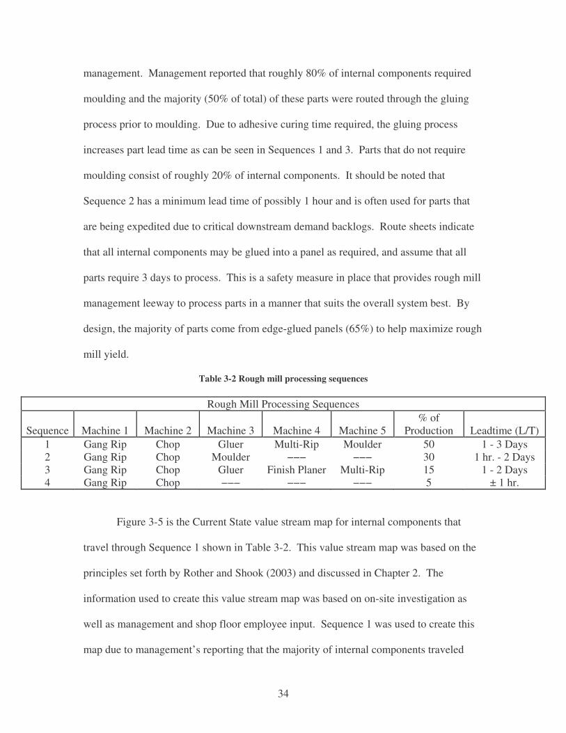
designed to be moulded. Table 3-2 was developed based on input from rough mill

34

management. Management reported that roughly 80% of internal components required

moulding and the majority (50% of total) of these parts were routed through the gluing

process prior to moulding. Due to adhesive curing time required, the gluing process

increases part lead time as can be seen in Sequences 1 and 3. Parts that do not require

moulding consist of roughly 20% of internal components. It should be noted that

Sequence 2 has a minimum lead time of possibly 1 hour and is often used for parts that

are being expedited due to critical downstream demand backlogs. Route sheets indicate

that all internal components may be glued into a panel as required, and assume that all

parts require 3 days to process. This is a safety measure in place that provides rough mill

management leeway to process parts in a manner that suits the overall system best. By

design, the majority of parts come from edge-glued panels (65%) to help maximize rough

mill yield.

Table 3-2 Rough mill processing sequences

Rough Mill Processing Sequences

Sequence Machine 1 Machine 2 Machine 3 Machine 4 Machine 5 % of

Production Leadtime (L/T) 1 Gang Rip Chop Gluer Multi-Rip Moulder 50 1 - 3 Days 2 Gang Rip Chop Moulder −−− −−− 30 1 hr. - 2 Days 3 Gang Rip Chop Gluer Finish Planer Multi-Rip 15 1 - 2 Days 4 Gang Rip Chop −−− −−− −−− 5 ± 1 hr.

Figure 3-5 is the Current State value stream map for internal components that

travel through Sequence 1 shown in Table 3-2. This value stream map was based on the

principles set forth by Rother and Shook (2003) and discussed in Chapter 2. The

information used to create this value stream map was based on on-site investigation as

well as management and shop floor employee input. Sequence 1 was used to create this

map due to management’s reporting that the majority of internal components traveled

35

through this machining sequence. The lead and value added times for the current state

value stream was based on observations an actual internal nightstand component order

(Table 3-3). Although the order shown in Table 3-3 is an actual order, the order number

(BBR#1) shown has been created to maintain confidentiality.

Table 3-3 Internal nightstand component order (BBR#1)

Nightstand - Bottom Back Rail

Length Width Thickness Material Grade # of

Pieces # of

Panels Total

Footage Lineal Feet

Rough 21’’ 23.25’

’ 1’’ Poplar 2 283 17.75 60 495

Finished 20.25’’ 1.25’’ 0.71875’’ − − − − − −

Table 3-3 is an example of the information that is found on a route sheet at the

study site. BBR#1 is a batch order for 283 bottom back rails that will be used in the

construction of a specific nightstand. This component’s final dimension and style has

been designed for 1 specific nightstand. Many other parts will used be along with order

BBR#1 for the final assembly of the nightstand. Rough dimensions (21’’ x 23.25’’)

reflect the panel dimensions required for panel glue-up. The number of panels shown

indicates how many panels are required for the multi-rip operation to obtain required 283

individual pieces of dimension size (20.25 x 1.25). Other information indicates rough

and finished thickness; material (species), part grade, total board and lineal footage for

the BBR#1 order. This order was selected to represent the internal nightstand

components to provide a common scale; nightstand order sizes vary due to forecasting by

the manufacturer and this order was reported to be a common order based on overall

component production.

36

Figure 3-5 Current State Value Stream Map

37

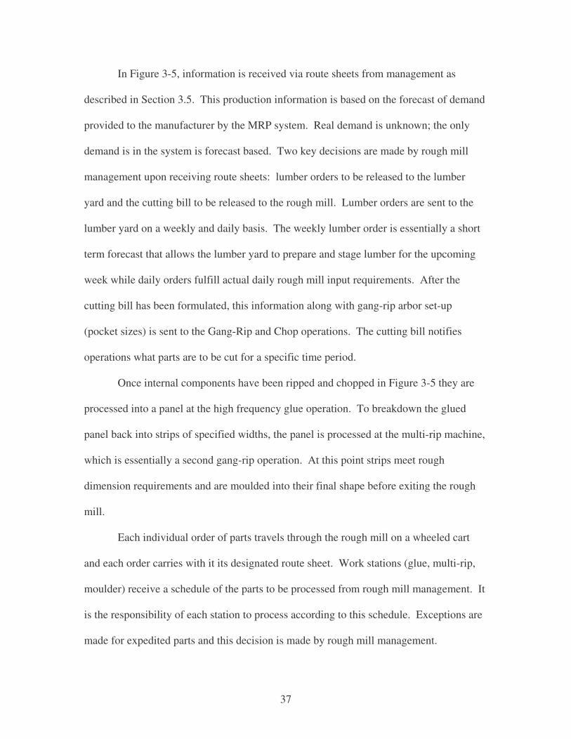
In Figure 3-5, information is received via route sheets from management as

described in Section 3.5. This production information is based on the forecast of demand

provided to the manufacturer by the MRP system. Real demand is unknown; the only

demand is in the system is forecast based. Two key decisions are made by rough mill

management upon receiving route sheets: lumber orders to be released to the lumber

yard and the cutting bill to be released to the rough mill. Lumber orders are sent to the

lumber yard on a weekly and daily basis. The weekly lumber order is essentially a short

term forecast that allows the lumber yard to prepare and stage lumber for the upcoming

week while daily orders fulfill actual daily rough mill input requirements. After the

cutting bill has been formulated, this information along with gang-rip arbor set-up

(pocket sizes) is sent to the Gang-Rip and Chop operations. The cutting bill notifies

operations what parts are to be cut for a specific time period.

Once internal components have been ripped and chopped in Figure 3-5 they are

processed into a panel at the high frequency glue operation. To breakdown the glued

panel back into strips of specified widths, the panel is processed at the multi-rip machine,

which is essentially a second gang-rip operation. At this point strips meet rough

dimension requirements and are moulded into their final shape before exiting the rough

mill.

Each individual order of parts travels through the rough mill on a wheeled cart

and each order carries with it its designated route sheet. Work stations (glue, multi-rip,

moulder) receive a schedule of the parts to be processed from rough mill management. It

is the responsibility of each station to process according to this schedule. Exceptions are

made for expedited parts and this decision is made by rough mill management.

38

Expedited parts are often the result of inaccurate upstream forecasting, unplanned

processing delays, and inaccurate inventory counts.

Between each process box shown in Figure 3-5 a black and white arrow exist

indicating that parts are “pushed” between each operation. The inventory triangle or WIP

held between each work station is shown below the “push” arrows. The number within

each process box represents the number of workers at each work station. The moulding

operation is the only operation which features the possibility of more than 1 machine

(currently 8 moulders are in place) being used for the production of internal nightstand

components indicated beside the moulder label in parenthesis in Figure 3-5. Below each

process box exists a data box, the data box contains the following information: cycle

time, changeover time, and uptime.

Flow time (F/T) was an additional measurement used at the moulders; flow time

represents the lead time when 1 moulder is used to process an entire batch. Due to batch

constraints, keeping an order confined to one moulder takes 19.8 minutes to process. If

the system was more flexible and the order could be distributed among the 8 moulders, it

could theoretically take 2.5 minutes. Typically 1 moulder to process a unit in order to

process an order. At the bottom of the figure lies a timeline which notes lead time and

value added time. The summation of lead and value added time is totaled on the bottom

right of the figure. BBR #1 (Table 3-3) of 60 board feet (BF) and 495 lineal feet (LF) of

internal components requires 15.1 hours (almost 2 business days) to be processed in the

rough mill while only 31.5 minutes of this time is value added time. Table 3-4 provides a

brief summary of the information found in Figure 3-5. It should be noted that the rough

39

planer/gang-rip/chop C/T was determined using 110.05 BF input due to rough mill

simulation results of 54.52%. This is discussed in detail in Chapter 4.5.

Table 3-4 Current state value stream map breakdown

Current state value stream map breakdown

Metric Rough Planer/Gang Rip/Chop High-Freq. Gluer Multi-Rip Moulder WIP 20 MBF 3376 BF 2442 BF 60 MLF

Throughput 2 MBF/hr. 1 MBF/hr. 750 BF./hr. 25 LF/min. Cycle Time 3.3 mins./unit 3.6 mins./unit 4.8 mins./unit 19.8 mins./unit

Changeover Time 15 mins. 20 mins. 6.5 mins. 23 mins. Uptime 70% 90% 80% 50%

Table 3-5 represents the labor as shown in Figure 3-5. Direct labor shown

represents the hourly labor employees while indirect represents supervisors on the floor.

Supervisors in some cases are shared resources, meaning they may be responsible for

more than one machine. This can be seen at the multi-rip and moulder. This information

was based on input from rough mill management, the industrial engineering department

and observation.

Table 3-5 Rough mill labor per machine per shift

Rough Mill Labor Per Machine per shift Machine Direct Labor Indirect Labor

Rough Planer 1 0 Gang Rip 2 0 Chop Saw 12 2

Gluer 5 1 Planer 2 0

Multi-Rip 2 0.5 Moulder (8) 2 0.375

3.7 Lumber Yard

Production begins in the lumber yard at the study site. Lumber is brought into the

lumber yard as green lumber from one of approximately 50 sawmill suppliers currently

40

used. At this point the lumber is graded to ensure the accuracy of the purchased grade

from the supplier. Once lumber has been graded and manually sticked, it is moved to a

holding area where it is airdried until demanded. Approximately 3.5 million BF of

lumber is held on the lumber yard for airdrying. The reason for holding this amount of

lumber is to remove moisture and help reduce the cycle time needed for the kiln drying

step. From the airdry storage site, the lumber will be staged for kiln drying. Airdrying

times can range from weeks up to several months. The amount of time spent airdrying

depends on lumber thickness and demand. Typically, as lumber thickness increases so

does the amount of time it will spend in the airdrying area. The time required to kiln dry

hardwood lumber is dependent on the lumber species, times can vary from 1 week to 3 or

more weeks. The furniture manufacturer operates 12 dry kilns with a total drying

capacity of 560 MBF. Once lumber exits the dry kilns and enters dry storage it is

physically ready to be staged into the rough mill for the lumber breakdown procedure.

3.8 The Rough Mill

The rough mill represents the first stages of lumber breakdown from kiln dried

boards into smaller pieces of wood that will make up the final furniture piece. At the

study site the following actions take place in the rough mill: rough planing, gang-rip and

chop, high-frequency gluing, finish planing, re-ripping and moulding. As seen in Table

3-2 not every internal nightstand component went through each of these actions. The

lead time designated by the company for the rough mill is 3 days and this is the standard

time used when determining the overall production schedule even though components

can be expedited in less time if needed (Table 3-2).

41

It should be noted that while internal nightstand components are the focus of this

study, many other parts are being processed through the rough mill at the same time.

Each machine in the rough mill is a shared resource. A shared resource means that no

machine in the rough mill is designated solely for the purpose of manufacturing internal

components. Hundreds of different parts create a 4/4’’ 2-C yellow poplar cutting bill and

the percent of internal components in a cutting varies on the schedulers forecast. Once

the rough mill was set up to run, it was observed that 4/4’’ 2-C yellow poplar was cut

typically 2-3 working days in a row.

3.8.1 Lumber Input

As mentioned, route sheets for each component order are produced by the MRP

system. Once route sheets have been produced, they are supplied to the rough mill 3

weeks ahead of the scheduled production start date. The rough mill supervisor collects

all route sheets due for a production week and separates them based on lumber

characteristics. For example, all 4/4’’ yellow poplar route sheets are grouped together

and all 5/4’’ yellow poplar bills are grouped together.

Route sheets do not indicate the time of the day parts are to be produced; they

only indicate production start date therefore grouping of route sheets is performed to

maximize yield by batching parts together and to increase productivity by limiting

changeovers at the rough planer and gang-rip operations. Changeovers at these stations

are required when lumber input characteristics differ such as thickness and or species.

The individual cutting bill tells the rough mill supervisor the board footage

requirement of the finished parts. To determine the lumber input needed to be input from

the lumber yard to the rough mill, the individual BF requirements from the route sheets

42

are summed and then a yield factor is applied. For example, if 1 batch of route sheets for

2-C yellow poplar individual component footage requirements totals 1 MBF; the rough

mill supervisor will order 2 MBF. The yield for 2-C yellow poplar in the rough mill has

been determined by management to be approximately 50%; this is why 2 MBF would be

input into the rough mill rather than 1 MBF. Once the BF required to fulfill cutting bill

requirements has been determined, the lumber yard will supply the lumber to the rough

mill.

3.8.2 Rough Planer/Gang-Rip/Chop Operations

This operation operates like a cell where the 3 pieces of equipment work together

as shown in Figure 3-5. Lumber advances from the lumber yard to the rough mill in

stacks via forklift. Between the lumber yard and rough planer roughly 18 MBF of

inventory is kept to feed the rough planer. The fork lift operator for the rough planer

must retrieve the lumber stacks from the lumber yard, stage stacks and feed the rough

planer at the same time. It was not observed during this study that the rough planer was

ever idle waiting for lumber. The forklift places stacks on a chain that feeds a Neuman

S282 planer. The basic human operations at this station are to unstack and destick the

stack and feed boards into the planer. Breakdown of the stack by the rough planer

operator is performed using a hoist and each board is manually taken from the top of the

stack and feed into the planer by the operator.

The rough planer is operated by 1 person and processing is first-in-first out (FIFO),

meaning whatever board comes to the planer operator first is the first board handled. The

planer has a 24’’ wide infeed and when the downstream gang-rip operation is running at

43

full capacity the planer operator has to feed the planer 2 boards at a time side-by-side to

maximize throughput to ensure the gang-rip is not starving for lumber.

The rough planer is paced by the gang-rip saw. If the gang-rip saw’s inventory

capacity is full, the rough planer must halt operations. Conversely, if the gang-rip

operation is starved the rough planer must increase production to satisfy the gang-rips

needs. It was observed during the study that the rough planer did not operate at full

capacity because the gang-rip operation was the bottleneck of the Rough Planer/Gang-

Rip/Chop operation. A conveyor and FIFO system links the rough planer to the gang-rip

saw therefore production matches the gang-rip. The inventory level between the rough

planer and the gang-rip was limited to the length of the conveyor system.

Changeover time for the rough planer to go to a different thickness was observed to

be 15 minutes. When a new species or thickness is ordered the planer operator must stop

operations. The operator must also wait until the downstream gang-rip and chop

operations cleared their systems of previous species or thickness before a new thickness

or species is planed; this is done to keep orders separated. Clearing the system was

observed to happen within the 15 minute changeover.

Lumber exits the planer and enters a Mareen Johnson fixed-blade gang-rip saw on

a conveyor. Just like the rough planer, the gang-rip operation is a FIFO process. There

are 2 operators at the gang-rip operation: one maintains the conveyor system and one

feeds the saw. One operator keeps boards exiting the rough planer to the gang-rip saw on

the conveyor and straight. This same operator also checks boards for quality and turns

the boards with the best face down. From here, boards continue to travel on the conveyor

to the next operator who uses a laser light to measure the maximum useable width of the

44

board based on the second best face. Defects such as wane are usually found on the

second best face and the best way get a true measurement of a board’s useable width is

by ensuring that this face is visible to the gang-rip operator. This measurement is used by

a computer control system to determine where the board will enter the gang-rip to

maximize the strip yield. The arbors in the gang-rip saw are spaced at varying pre-set

intervals determined by the cutting bill to maximize yield.

To maximize strip yield, a standard 4/4’’ 2-C yellow poplar arbor spacing sequence

(Table 3-6) was developed at the study mill using past cutting data. The purpose for

having this standard arbor is to maximize yield and decrease downtime from arbor

changeover. 4/4’’ 2-C poplar is roughly 24% of production therefore minimizing

downtime from changeovers which take 10 -15 minutes is required to maximize

throughput. As can be seen in Table 3-6 the widest 4/4’’ piece that can be obtained from

the standard arbor is 2 ¾’’ and the narrowest piece attainable is 1 3/8’’.

Table 3-6 Standard 4/4’’ 2-C Poplar Arbor used by study mill

Standard 4/4 Poplar Arbor Arbor Pocket Size

1 2 3/8'' 2 2 3/4'' 3 2’’ 4 1 3/8'' 5 2 3/8'' 6 2’’ 7 2’’ 8 2 3/4'' 9 1 3/8''

10 1 3/8''

For all cuttings on the gang-rip that are not 4/4’’ 2-C poplar, different arbor set-ups

are made depending on the order or bill. The arbor set-up for a non 4/4’’ 2-C poplar

45

order is formulated in the production office based on part size requirements from the

route sheets. The arbor is built ahead of time by employees in the tooling room. Once

the arbor has been built the changeover is performed by the same gang-rip operator that

feeds lumber into the machine. This changeover occurs within the 15 minutes allotted for

planer set-up time. The saw kerf produced by the saw blades is 3/16’’. Once pieces have

been ripped out by the gang-rip saw they travel on a conveyor to the chop saw operation.

The current throughput goal of the rough mill set by management is 2 MBF

through the gang-rip per hour for 4/4’’ lumber, this goal was observed to be met when no

lengthy changeovers occur when switching species. The only gang-rip downtime

observed was when waiting for the downstream chop operations. Downstream chop

operations can manually turn off the gang-rip line when too much lumber accumulates in

their small buffer area.

Strips come from the gang-rip saw on a conveyor belt to the chop saw operation.

The chop saw is a Barr Mullin Wondersaw brand chop saw. Between the gang-rip and

chop saw is a FIFO process. The purpose of the chop operation is to cut out unacceptable

wood features and cut pieces to required lengths. The defecting process involves

approximately 6 workers using fluorescent crayons to mark unacceptable features in the

lumber strips that need to be removed by the chop saw. Typically 2 marking workers

will operate 1 line. What determines constitutes a removable feature differs between

species and is based on the final part end use. An internal component that will go unseen

in a furniture piece is allowed to have more “features” than a piece that will be seen on

the outside. Markers are instructed how to defect based on cutting bill requirements by a

supervisor. Once a strip has been marked for removable features it is sent to the chop

46

saw where the strips will be automatically chopped using a computer vision system that

identifies the fluorescent mark on the strip and cuts out the marked section of the strip.

In addition to defecting, the chop saw also cuts the strips to part length

requirements. These part length requirements to fulfill orders based on cutting bill

requirements that are programmed to the chop saw scanning system. Essentially, the

scanning system first identifies marked sections to cut out of a strip and then determines

what part length to cut out of the remaining “acceptable” length of a strip. As several

hundred lengths and quantities per length may be required to fulfill a cutting bill,

emphasis on which part lengths to be cut at the chop operation differs.

Greater priority is placed on longer lengths than shorter lengths. Greater

emphasis is placed on longer lengths because these orders are considered to be “harder”

to fulfill. For example, it is easier to obtain a feature-free part length of 40’’ than is it a

defect-free part length of 60’’ therefore the scanning system first searches for a part of

60’’ and if that length is not obtainable it will search for a part of 40’’. While this

process of placing greater emphasis on longer pieces may increase yield it places less

emphasis on actual part demand. A piece that is of smaller length may be in more

demand however this piece may be passed over routinely by the scanning system because

greater emphasis is placed on longer lengths.

Once strips have been defected and cut to length, parts of a specific length and

width are then routed to a designated off-loading station where 6 more workers are

assigned specific part dimensions to unload. The worker assigned to the specific part

unloading station will then load the parts onto a cart until the order requirements are

fulfilled. Once the part requirements have been fulfilled, parts will be removed from the

47

chop saw cutting options and a new part will be inserted into its place and the cycle

repeats.

In many cases, part width requirements can not be met. This occurs for various

reasons such as: arbor pocket size does meet specific part requirements or less emphasis

was placed on the obtaining the piece as a solid piece at the chop saw. When parts width

requirements can not be meet, random width parts of the same length are edge-glued

together into panels.

3.8.3 Edge Gluing Operation Parts that come from the gang-rip line are either too small (less than 1 ¼’’) or

large (2 ¾’’) or if not enough parts come from the gang line as solid to fill an order. The

arbor pocket size also determines if parts will be glued into a panel. Obviously if a part

width requirement is wider than the widest pocket, random widths will be cut from cut

off saw at the required length and subsequently glued into a panel to allow for re-ripping

downstream to the desired width. The difficulty of the cutting bill and the range of part

sizes also play a role in whether a part will be glued or taken solid from the gang-rip.

Parts are staged after the chop line on carts in a designated area while waiting to

be glued. While several types of edge-gluing operations exist at the study site, internal

nightstand components are strictly routed to the Rosenquest machine. The Rosenquest is

a continuous edge gluer; meaning one continuous core is produced and then cut off at

specific lengths. It takes 5 operators to run the machine. Two operators stage a group of

10 or so parts by feeding the parts across a glue applicator on edge. The next 2 operators

take the parts off of the glue applicator and feed the parts edge to edge continuously into

the machine where the resin is cured. A chop saw resides on the exiting side of the

48

machine that cuts the continuous panel to length as indicated on the route sheet. From

here, the newly sized panel is off-loaded onto a cart by the 5th operator. At this point, the

panel proceeds downstream to be re-ripped at a Multi-Rip machine into the strip width

that was previously unattainable at the gang-rip operation. The throughput for the

Rosenquest was observed to be 1 MBF/hour.

3.8.4 Multi-Rip Operation

The multi-rip operation is essentially a gang-rip operation in that panels are fed

through a multiple blade saw. Using the same principles as the initial gang-rip system,

arbors in the machine are set to cut strips of specific widths out of a panel. These arbors

must be changed frequently depending to meet part width requirements and fulfill the

route requirements. The multi-rip machine is operated by 2 workers: 1 operator feeds

glued panels into the machine while the other removes the strips and places them onto a

cart. Throughput at the multi-rip was observed to be 750BF/hour and a recent study by

management determined that changeover is 6.5 minutes.

3.8.5 Moulders

Currently eight Weinig moulders are in place at the study site. Each moulder has

2 operators; 1 in-feed and 1 out-feed. The moulding operation is considered by most to

be the bottleneck of the study rough mill. Changeovers are frequent and fairly lengthy at

this operation. During observation it was apparent that the machines were operated at

approximately 50% uptime. Management felt the moulding operation could lengthen part

lead time by 1 day if downtime was not minimized.

49

Much like previous operations, part orders are grouped together at this point if

possible. Part grouping is not possible if the designed mould differs between orders.

Moulders operate only on the first shift due to the importance of this process and lack of

second shift supervision. Changeover times at the moulder operation often vary between

each moulder. Depending on operator experience and ability to properly set-up up the

machine changeover times differ, however it was observed that an average changeover

consumed approximately 23 minutes. This information was based data on obtained from

past improvement events and data collection by the manufacturer.

Batches are kept together through 1 moulder and not split to different moulders.

Batches are routed though to specific moulders based on availability and specific finished

thickness. A recent improvement event assigned each moulder specific part thicknesses

in hopes of decreasing downtime and creating standard work (Table 3-7). For example, if

a part requires a finished mould thickness of 15/16’’ it would be routed to either Moulder

# 2, 3, 5 or 6. Throughput for each individual moulder was measured to be 25

LF/minute; this was based on observation and data collection by the manufacturer.

Table 3-7 Moulder assignments

Moulder Part Finished Thickness 1 3/4'' − 2 15/16'' 1 5/8'' 3 15/16'' 13/16'' 4 3/4'' 15/16'' 5 15/16'' 1 5/8'' 6 15/16'' − 7 Any Any 8 Expedited and Sample Parts

50

3.9 Yield Fifteen 4/4’’ 2-C poplar cutting results were taken to determine yield results

(Figure 3-6). The cutting results were taken from the manufacturer based on output

provided by the Barr-Mullins Scanning System. A yield of 55% is the current

benchmark for 4/4’’ 2-C poplar in the rough mill. The average yield of the 15 cuttings

during the case study was 57.74%. Rough mill management uses a rule of thumb of 50%

yield which differs from the benchmark and actual results. Management was unable to

track of which parts were obtained solid and which would have to be subsequently glued.

The only measurement obtained from the software was the yield result even though

additional information may have been available. Yield is the most important metric at

the study rough mill however this metric is only known by management. Furthermore,

the yield measurement used by management comes from the Barr-Mullins scanning

system report. This yield may or may not be a good measure of actual rough mill yield.

Figure 3-6 Yield Results from 15 4/4’’ 2-C poplar cuttings

4/4 Poplar Yield

50

52

54

56

58

60

62

64

1 2 3 4 5 6 7 8 9 10 11 12 13 14 15 Consecutive cuttings

%

51

The yield results are observed quickly with no discussion as to why the

measurement was obtained or how to improve it. Lumber costs drive the focus of the

measurement. At the study site, the success of the rough mill’s performance is based on

its ability to meet or exceed the benchmark established for this metric.

3.10 Work Time

Table 3-8 shows the available work time in the study rough mill. As can be seen,

employees work four nine hours shift Monday through Thursday and 4 hours on Friday.

The rough mill operates a full first and partial second shift; the rough planer, gang-rip,

chop and 2 gluers operate on second shift. Management noted that on occasion the finish

planer and multi-rip operate on second shift however this is seldom. The gluing

operations on second shift do not include the high-frequency gluer used to produce

internal components. To address order backlogs it is not uncommon for overtime to be

performed which includes weekends. Including the rough mill manager and 4

department supervisors a total of 101 employees work in the rough mill. Rough mill

employee’s job experience ranges from 2 to 40 years.

Table 3-8 Available Work Time in Rough Mill

Time Available Actual Available Work Time Hours Minutes Paid Break (mins) Hours Minutes

Monday 9 540 20 8.67 520 Tuesday 9 540 20 8.67 520

Wednesday 9 540 20 8.67 520 Thursday 9 540 20 8.67 520

Friday 4 240 10 3.83 230 Total 40 2400 90 38.50 2310

52

3.11 On-Time Delivery

Past production schedules and input from with the manufacturer’s industrial

engineer was used to determine the rough mill success in meeting scheduled delivery

times to downstream processes. The rough mill’s ability to meet on time delivery to

downstream demand was observed to be the rough mill supervisor’s main concern; if the

schedule is not met in the rough mill, all downstream processes suffer. The rough mill

supervisor was observed to be under great pressure to meet downstream needs even

though much of the rough mill’s success was determined by the rough mill’s ability to

meet the set yield metric. No on-time delivery metric was used by the rough mill

supervisor to gauge success in meeting downstream demand.

Through the industrial engineering department in the main office, information was

made available to estimate the rough mill’s on-time delivery to internal customers.

Figure 3-7 represents the rough mill’s on-time delivery percentage for 9 weeks of

production. This was determined using the manufacturer’s “off-schedule”. The off-

schedule is a production schedule that contains orders that are being produced behind

their respective original schedule date. Orders on the off-schedule are the result of the

rough mill’s inability to meet the schedule’s requirements. The rough mill could not

produce these orders according to the original schedule therefore they were moved to the

off-schedule. Recovering the off-schedule while producing scheduled items is a difficult

feat, as can be seen from Weeks 1 through 6. Once the manufacturer gets behind with an

off-schedule, the on-time delivery percentages decrease in the following weeks.

53

% O n-Time Delivery

0

20

40

60

80

100

1 2 3 4 5 6 7 8 9

W eek

%

Figure 3-7 Timeline of on-time percentages based on the “off-schedule”

The lowest on-time delivery percentage obtained was 53% which occurred in both

weeks 4 and 5. On-time delivery increased in week 7; however, this week was a holiday

week and generally the scheduler keeps production at a minimum during holiday weeks.

This allowed the rough mill to recover the off-schedule. In week 9, on-time delivery

reaches a much improved 96%; however, this is the result of the manufacturer

undergoing a production “re-schedule”.

A re-schedule is a production schedule change provided by the scheduler that

virtually eliminates the off-schedule. In a re-schedule, off and on schedule products

production start dates are pushed back to remove the off-schedule. In some cases

products that might have been scheduled for manufacture may be removed and replaced

with products from the off-schedule. Since all products previously on the off-schedule

have been given a new belated production start date the rough mill can increase on-time

delivery percentages. A re-schedule is made possible since the original schedule is a

54

forecast; no products are in actual demand by the final furniture customer. Re-schedules

effect all processing at the manufacturer, not just the rough mill. The process of a re-

schedule was observed to be chaotic for management and production actually halted.

Production in the rough mill stopped during the study period and workers were sent home

to avoid working ahead of schedule. The implications of a re-schedule on overall rough

mill effectiveness has a significant impact, but this impact is beyond the scope of this

study.

3.12 Current State Improvement Opportunities

Many improvement opportunities exist for the rough mill however for the purpose

of this study they were limited to: overproduction, unnecessary inventory, waiting,

inappropriate processing, defects, transportation and motion. Identifying these areas of

opportunity in the Current State will provide focus points in the design and evaluation of

the Future State value stream maps (Chapter 4). Opportunities for improvements were

found based on observation and employee input.

3.12.1 Overproduction

Overproduction provides the greatest opportunity for improvement in the rough

mill and is often the root cause of waste in most manufacturing settings (Rother and

Shook 2003). Overproduction exists at the study site due to the nature of production

scheduling currently in place. Like most mass production models the current state

schedules production at multiple points throughout the rough mill. Each scheduling

location, or machine operation, produces to a forecasted schedule and then pushes the

products downstream to the next machine where the products must be recounted and

55

staged until that particular’s machine schedule indicates production. By producing to a

forecast and pushing products through the system waste can occur in: unnecessary

inventory, waiting, inappropriate processing, defects, transportation and motion. For this

reason, overproduction has been labeled the root cause of manufacturing waste. The goal

of the rough mill should be to schedule production at one point based on actual demand

and produce only to replenish consumed parts to alleviate manufacturing wastes

associated with overproduction.

3.12.2 Unnecessary Inventory

Unnecessary inventory is the result of overproduction. By producing too early

and pushing parts through the rough mill from one machine to another based on multiple

schedules, WIP levels of undemanded products increase. This inventory must be re-

counted and stored which results in additional manpower cost and production time. By

scheduling at one point based on demand, unnecessary inventory is not produced initially,

but only when needed, which should be the goal of the rough mill.

3.12.3 Waiting

Due to the lack of any systematic product flow, orders throughout the rough mill

are disorganized and workers could spend as much as 15 minutes locating which order to

process next. Work in progress for each machine is held in a specific location generally,

however that location may not be right beside machine and often several areas were used

to hold one machine’s WIP. As WIP levels increased, the disorganization of the rough

mill increased creating less flow and more downtime in finding the right orders to

process.

56

It was not observed that workers spent time waiting on orders to process. If an

order on the schedule was not ready, supervisors were notified and the workers continued

onto the next batch of parts, possibly producing ahead of schedule further adding to

unnecessary inventory. Machine utilization requirements dictated that if a scheduled

order could not be found, then any order in WIP would be processed to avoid a machine

being idle. Running orders out of sequence further reduces the ability of meeting

downstream demand on-time. WIP for a specified machine in the rough mill should be

kept at one standard location to eliminate time spent locating orders throughout the rough

mill and to prevent producing ahead of schedule.

3.12.4 Inappropriate Processing

What determines inappropriate processing can be defined as processing that is

considered to be value added or non-value added. Value added processing is considered

appropriate processing, while non-value added processing is considered inappropriate

processing. In the Current State value stream, 4 processing steps take place to produce

internal components of which 2 are considered value added (rough planer/gang-rip/chop

and moulding operation) and 2 are considered non-value added (edge gluing and multi-

ripping). These 2 non-value added operations were deemed necessary by management to

increase yield thus reducing lumber costs. But, these extra steps add cost and are not

essential for the function and form of internal components. The goal of the rough mill

should be to decrease inappropriate processing (non-value added processing) whenever

possible. Inappropriate processing does nothing to add value to the final product form

that could not be accomplished with the primary rough mill operations and only increase

lead time and decrease the rough mill’s ability to meet downstream demand.

57

3.12.5 Defects

Overproduction hides defects in products until the downstream processes use the

part which results in shortages. When an order does not contain the required amount, a

new batch of parts must either be expedited back through the system or pulled from

another order. The further an order gets through the rough mill before employees notice

a shortage the more complex and problematic it can be to find the source of problem and

to expedite parts.

To prevent shortages, an overage factor is applied to each part order by the MRP

system. At each specific machine, there is a chance that a small percentage of the parts

that enter the machine will not exit the machine in an acceptable state (due to quality

issues). Machine errors such as moulder bites or improper machine set-up may cause

parts to be deemed unacceptable and therefore these parts must be set aside and not

processed further.

Table 3-9 Overages example according to MRP

MRP Overages Machine Part Requirements (MRP) Overage

Gang-Rip/Chop 165 10 Gluer 160 5

Multi-Rip 158 3 Moulder 155 �

Actual Part Requirements 155 �

Table 3-9 is an example of the spoilage factor the MRP system applies to

determine the number of parts each machine requires to meet the actual part requirement

of 155. As can be seen, the Gang-Rip/Chop operation must produce 165 parts to ensure

that the subsequent machines have enough parts to fulfill the order. It is assumed that 10

parts will be “spoiled” during all steps in rough mill manufacturing. Current

58

management was unsure of how the spoilage factor was determined or adjusted as the

factors were created more than 20 years ago.

When parts are not spoiled as according to the MRP, these extra parts are

disposed before they exit the rough mill. In the example in Table 3-9, if no parts are

spoiled, then 10 parts are thrown away. This means that the extra work in processing,

transporting those 10 parts are wasted. When the spoilage factor does not cover the

degree of machine and human error, part shortages occur.

An order that is short on parts is bypassed and moved to the side until the shortage

is rectified. This delays the schedule as orders that were supposed to be processed at a

later time are being processed early while the scheduled order falls even further behind.

The entire rough mill can be off schedule due to shortages, especially if the lumber input

in the rough mill at the rough planer must change over to accommodate for expedited

orders.

Lumber input changeover due to expediting was not observed to occur during the

study however management indicated that the possibility exists. In the case that multiple

part orders of the same species fell short of requirement, these orders would be moved off

the schedule until the next time that particular lumber species was pulled from the lumber

yard. It is difficult to accurately obtain, track and maintain the correct number of pieces

and ensure these parts remain on the cart while being transported through and stored in

the rough mill.

3.12.6 Transportation

Because of overproduction and inappropriate processing, transportation in the

rough mill is extensive, part orders must be moved continuously to make room for more

59

orders. Parts travel through the rough mill on wheeled carts (approximately 3’ x 5’).

Management discovered parts may travel as much as 1.5 miles on carts before exiting the

rough mill. These carts are old, heavy and create clutter. Due to the design of the rough

mill, these carts are moved excessively and oftentimes moved solely for the purpose of

creating space for more carts. The majority of floor space in the rough mill consists of

these carts.

Generally each cart in the rough mill holds the parts to fulfill one order

requirement. As the study site decreases order size and increases order variety, issues

concerning cart usage and part transportation flexibility may increase. Decreased order

size results in carts not being filled to their full capacity to keep orders separate and

increased order variety yields increased the number of carts. The number of carts in the

rough mill is already at an observed maximum and the number currently in place should

only decrease. The goal of the rough mill should be to reduce part transportation

throughout the rough mill by providing a central location for WIP holdings. Locating

orders in an organized and standard manner, the chance of orders being transported 1.5

miles through the rough mill can be reduced.

3.12.7 Motion

Wasted motion in the rough mill is the result of inappropriate processing.

Because the manufacturer produces to a forecast it is entirely possible for the

manufacturer to produce a piece of furniture that will not be sold. Unless the

manufacturer is producing to fulfill immediate customer demand the act of forecasting

creates a wave of excess motion in actual manufacturing. Every action that takes place in

manufacturing, whether value or non-value added, is performed based on the belief that

60

customers desire the product being produced. If ultimately the customer does not

demand the product after final manufacturer, then even the value added steps throughout

the system would be considered waste in motion. The previously mentioned

improvement opportunities affect the amount of motion in the rough mill currently and

focusing on these areas will decrease the amount of excess motion. Addressing this issue

of linking actual demand to production scheduling is critical for ultimate business

success, but is beyond the scope of this study.

3.12.8 Opportunities Summary

As shown, opportunities exist for the current state to better respond to downstream

demand by eliminating processing waste. The following chapter will focus on rough mill

system design that will target each of the previously mentioned wastes. Ultimately, by

reducing these wastes the rough mill will be able to better serve downstream demand

appropriately. The priority of the future state value stream maps discussed in Chapter 4

is to ensure customer demand is met, first, and then it will be evaluated in terms of cost

effectiveness.

61

4 Rough Mill Future State Evaluation

4.1 Introduction

The purpose of this chapter is to describe a methodology to create improved rough

mill value streams. A case study was used to evaluate the cost effectiveness of two future

state value stream maps for the study site’s rough mill using pull production techniques.

The future state value stream maps are based on opportunities from the current state value

stream evaluation performed in Chapter 3. Just as in Chapter 3, the future state value

stream maps were based on internal nightstand component order BBR#1 (Table 3-3) and

processing sequence #1 (Table 3-2).

The purpose of pull system implementation is to reduce overall lead time at the

furniture manufacturer and increase on-time delivery from the rough mill to downstream

furniture operations. A yield analysis was performed using the ROMI-3 (Weiss and

Thomas 2005) simulation program on the current and both future state value stream

cutting bills to quantify and account for differences in yield.

4.2 Methods

The second objective involved the development of two future state value stream

maps (Future State #1 and Future State #2) based on the findings from the Current State

evaluation (Chapter 3). Both future state value streams were developed using the same

product as the Current State, internal nightstand component order BBR#1 (Table 3-3).

The purpose of future state value stream mapping was for the development of a pull

based system to better link production with demand; this was accomplished with the

implementation of supermarkets.

62

The amount of inventory to be held in supermarkets was based on the total internal

nightstand component piece production in 2006. All production data was obtained from

the furniture manufacturer. Internal nightstand components vary between each finished

nightstand style in dimension and part grade therefore previously mentioned ABC part

analysis was used to determine which components level will be held in the supermarket

and respective inventory levels. Supermarket inventory levels were determined by using

Smalley’s (2004) formulas for cycle, safety, and buffer stock.

To determine the effects of yield in the Future State value stream maps ROMI-3

(Weiss and Thomas 2005) simulation was used. Using simulation, a model was created

to validate the current state value stream. Validation was determined by simulating an

actual cutting at the furniture manufacturer. Part yield results from both the manufacturer

and simulation were compared. Using the validated current state simulation, changes in

the future state value stream were simulated to determine effects on yield.

Future State value #1 remained similar in processing activities as the Current State.

However, Future State #2 was designed based on the elimination of inappropriate

processing waste found in the Current State evaluation in order to decrease lead time and

increase on-time delivery to downstream demand. The effects of the supermarket based

pull system on manufacturing waste found in Objective 1 are discussed.

4.3 Future State Value Stream Mapping

The purpose of current state value stream mapping is for further development of

future state value stream maps. Using the findings from the Current State evaluation

(Chapter 3), future state value streams can be developed using pull techniques to limit

overproduction. As mentioned, overproduction is the root cause of not meeting

63

downstream demand (Chapter 3.12.1). Overproduction prohibits meeting downstream

demand in a timely manner by tying up the system with products that are not in current

demand.

To reduce overproduction, supermarkets of parts have been implemented into both

rough mill future state value maps to pull and control production. Supermarkets maintain

standard predetermined levels of finished goods which are based on normal variations in

past demand. As parts are removed from the supermarket, a kanban signal which

describes the type, quantity and processing method regarding parts removed from the

supermarket is sent to upstream production for supermarket replenishment. This

eliminates problems arising due to production forecasting and multiple scheduling points

which currently exist in the rough mill and limit it’s ability to meet downstream demand.

The standard types of inventory held in the supermarket are: cycle, buffer and

safety stock (Figure 4-1). As can be seen in Figure 4-1, cycle stock covers average

weekly demand, buffer stock, and safety stock is in place in the supermarket if actual

demand is greater than the cycle stock. Demand changes can be observed by monitoring

weekly supermarkets inventory levels and inventory levels can be adjusted accordingly to

avoid stock-outs and overproduction. The details of how the supermarket is applied in

this case study are discussed further in Chapter 4.4.

Future State value stream #1 does not represent a big change in the rough mill. It

utilizes the supermarket concept discussed above to address many of the issues discussed

in Chapter 3.12, particularly to provide limits to help control overproduction. The lead

time of this proposed value stream system has not been improved but the ability to

respond to downstream demand has been addressed. Non-value added activities have not

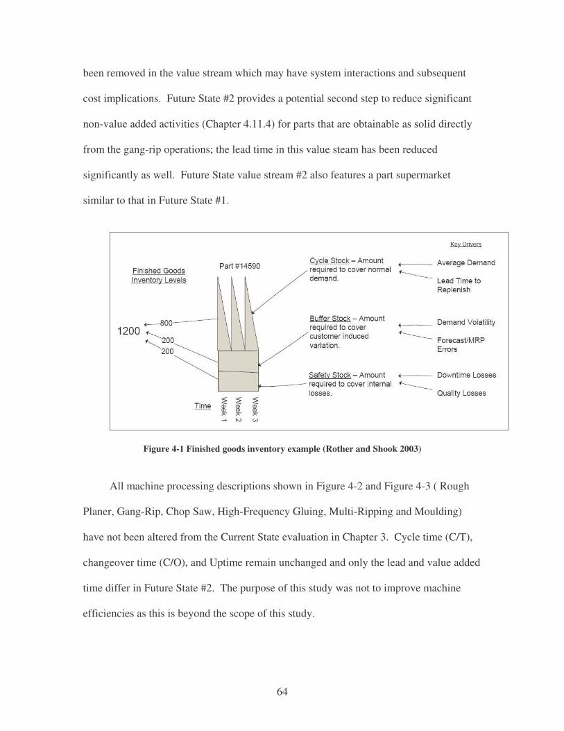
64

been removed in the value stream which may have system interactions and subsequent

cost implications. Future State #2 provides a potential second step to reduce significant

non-value added activities (Chapter 4.11.4) for parts that are obtainable as solid directly

from the gang-rip operations; the lead time in this value steam has been reduced

significantly as well. Future State value stream #2 also features a part supermarket

similar to that in Future State #1.

Figure 4-1 Finished goods inventory example (Rother and Shook 2003)

All machine processing descriptions shown in Figure 4-2 and Figure 4-3 ( Rough

Planer, Gang-Rip, Chop Saw, High-Frequency Gluing, Multi-Ripping and Moulding)

have not been altered from the Current State evaluation in Chapter 3. Cycle time (C/T),

changeover time (C/O), and Uptime remain unchanged and only the lead and value added

time differ in Future State #2. The purpose of this study was not to improve machine

efficiencies as this is beyond the scope of this study.

65

4.3.1 Future State Value Stream Map #1

As mentioned, Future State value stream map #1 (Figure 4-2) is similar to the

current state value stream map with the addition of a part supermarket as well as FIFO

(First-In-First-Out) lanes. Both value stream maps lead and value added times are based

on the example order (BBR#1) (Table 3-3) found in Chapter 3.6.

The part supermarket has been implemented in front of the moulding operation.

This location for the supermarket was based on constraints presented by varying finished

component moulding styles. By placing the supermarket upstream from the moulding

operation, internal components can be kept in a rough blank state and then moulded to

fulfill certain style requirements as needed. The number of differing moulding styles

would significantly increase the size of the supermarket if located downstream from the

moulding operation.

The implementation of the supermarket means the moulder operators simply pull

the required blank pieces from the supermarket immediately as indicated by the “part

schedule and moulding requirements” information provided. As parts are pulled from the

supermarket, the multi-rip machine operators notify management of parts withdrawn for

supermarket replenishment by kanban cards. This signals the rough planer/gang-rip/chop

cell to produce the withdrawn parts during the next 2-C poplar cutting. First-In-First-Out

lanes have been put into place for quality issues, the longer a part sits on a cart the greater

the potential for spoilage. Basically, the FIFO lane dictates a standard predictable and

visual route for internal parts through the system to ensure easy tracking of parts to be

replenished. Also in Future State #1, the part schedule and moulding requirements are

66

sent directly to the moulders eliminating possible schedule alterations by management

and allowing for production to be based on downstream MRP based demand.

Figure 4-2 Rough mill Future State Value Stream Map #1

67

4.3.2 Future State Value Stream Map #2 Future State #2 (Figure 4-3) is a simplified version of Future State #1 where only

value-added activities exist to supply the part supermarket reducing inappropriate

processing. For this to be possible, Future state value stream #2 requires that the gang-rip

and chop operations obtain the correct part width and length to avoid necessary non-value

activities associated with panel production. The supermarket analysis in Chapter 4.4

found that some internal components can not be obtained as solid from the gang-rip

operation because their dimensions were greater than any of the standard arbor pocket

sizes used at the study site for 2-C yellow poplar cuttings. Due to these arbor limitations,

panel production would be considered a necessary non-value added activities in this case.

These parts must be routed through Future State value stream #1; this routing is

represented in Figure 4-3 by two supermarket symbols.

By removing the non-value added processes, information flow and processing

documentation throughout the system has been decreased. Just as Future State #1, as

parts are withdrawn from the supermarket, the kanban signal is sent to rough mill

management for replenishment during the next poplar cutting. The flexibility of Future

State #2 is greatly increased by eliminating processing steps; not only will the

supermarket be able to supply downstream processes with the parts efficiently but the

lead time to replenish the supermarket is reduced as well. Because machines require

maintenance and occasionally may be non-operational the predictability of Future State

#2 is greater than both the Current and Future State #1. The overall lead time was

reduced by more than half of the Current State and Future State #1. The effects of

eliminating the panel glue-up activities are discussed in Chapter 4.5.

68

Figure 4-3 Rough mill Future State Value Stream Map #2

4.4 Supermarket

As mentioned, both future state value stream maps were developed using

supermarkets of internal components. Supermarkets are areas on the shop floor which

69

hold small levels of controlled inventory (Chapter 2.4.2). Inventory levels and which

items are held in the supermarket was based on 1 year of past production figures provided

by the manufacturer. A items represent 60% of demand and represent those parts that are

ordered frequently. B items constitute 20% of the total demand past A items, these items

are demanded frequently but not as frequent as A items. C items account for the

remaining items produced. C items are considered to be ordered infrequently and in

highly variable amounts (Smalley 2004). Orders for parts held in the supermarket receive

first priority since the orders are based on actual demand. All other MRP based orders

will be processed accordingly since a 3 day leeway has been built into the system to

process orders.

4.4.1 A, B, C Analysis

The 2006 nightstand production line consisted of 58 nightstand styles that are

constructed using 210 different internal component nightstand styles or Stock Keeping

Units (SKU). From the 210 SKU’s used during 2006 year, 109,858 individual internal

components were produced. In order to minimize the number of varying SKU’s in the

supermarket, parts of similar dimensions were grouped together. As seen in Table 4-1, it

is possible for differing SKU’s to have the same physical characteristics but be been

given different SKU’s. The quantity and SKU are the only differing features between

parts. Table 4-2 is an example of part grouping based on the differing SKU’s shown in

Table 4-1. The SKU’s have been eliminated and part quantities summed.

Table 4-1 Differing SKU's with identical physical characteristics

SKU # Length Width Thickness Quantity

12607 20’’ 1.5’’ 4/4’’ 165 28995 20’’ 1.5’’ 4/4’’ 200

70

Table 4-2 Part grouping based on Table 4-1

Length Width Thickness Quantity 20’’ 1.5’’ 4/4’’ 365

To further reduce the amount of individual part groups, downstream machine

capabilities were taken into consideration. Moulders are capable of handling rough parts

up to 3/8’’ wider than the finished dimension. Machines downstream from the rough mill

are capable of handling parts up to 2’’ longer than the specified finished length. Rough

mill management noted that often parts exit the rough mill with a length and width

greater than design indicated and does not effect quality or process speed. Taking this

into consideration, groups that have previously been limited to specific lengths and

widths were grouped further into “ranges” of lengths and widths as seen in Appendix 1

and Appendix 2. Appendix 1 and Appendix 2 is the determined A and B part widths and

lengths to be held in the supermarket for both future state supermarkets and the total

quantity of parts produced in 2006. Part widths have been separated based on the gang-

rip saws ability to obtain parts as either solid or glued. Component part grades (Grade 1

and Grade 2) were also used in the part analysis. Part Grades 1 and 2 are discussed in

Chapter 4.5.1.

As mentioned in Chapter 4.3.2, due to fixed-blade gang-rip, the widest part that

can be obtained is 2 ¾’’. The supermarket size was not limited to this constraint in the

Future State #2, even though the gluing process has been removed. Some parts contained

in the supermarket for Future State #2 must be routed through the gluing process. The

purpose of this study was not to provide a new arbor spacing sequence therefore the

current state arbor setting will remain unchanged. In this study, any part dimension that

71

is not within Appendix 1 and Appendix 2 is considered a C component and must be made

to order. These parts are given greater priority and processed before supermarket

replenishment stock. A total of 10 parts were classified as “A” components and 19

components were classified as “B”. Order BBR#1 (Table 3-3) which all value stream

maps were based upon is considered an A component.

4.4.2 Supermarket Inventory Levels

The part dimensions shown in Appendix 1 and Appendix 2 are the parts to be held

in the supermarket. The amount of finished goods to be held in the supermarket was

determined using Smalley’s (2004) calculation. Smalley’s calculation is the summation

of cycle, buffer and safety stock (Table 4-3).

Table 4-3 Finished goods inventory level calculation

Cycle Stock + Buffer Stock + Safety Stock =

Finished goods inventory level

Cycle stock according to Smalley (2004) is “average daily demand multiplied by

the lead time to replenish (days)”. To determine the cycle stock of the selected internal

components, the total annual amount of parts produced in each dimension category in

Appendix 1 and Appendix 2 was divided by the total number of work days (240) for the

year 2006. The lead time to replenish used to determine cycle stock was 5 days, or

essentially 1 work week. This lead time was used because the rough mill under study

typically only processes 4/4’’ 2-C yellow poplar in one batch 1 time per week and parts

of similar dimensions are grouped together when batched.

72

Buffer and safety stock exist in the supermarket to reduce the chances of

supermarket depletion. Buffer stock is percentage of the cycle stock to cover normal

demand variation (25%) (Smalley 2004) while safety stock is a percentage of both cycle

and buffer stock. 20% of cycle and buffer stock was used for safety stock. Because

demand variation from the manufacturer was unavailable, Smalley’s (2004) example for

buffer and cycle stock calculations was used. Table 4-4 is an example of how finished

goods inventory levels were determined for the part dimensions shown in Appendix 1

and Appendix 2. The example in Table 4-4 reflects how finished goods were calculated

for the part dimension group of 25.25’’ - 27.25’’ in length and 1.188’’ - 1.563’’ in width

and Part Grade 1. Table 4-5 and Table 4-6 are the determined finished good inventory

levels for A and B components.

Table 4-4 Finished good inventory level example

Finished Goods Inventory Level Example for 1 Part Dimension Annual Production 4373 Total parts −

Cycle Stock Daily Demand x 5 Days 91 Buffer Stock 25% x Cycle Stock 23 Safety Stock 20% x (Cycle and Buffer Stock) 23

Total Quantity Cycle + Buffer + Safety Stock 137

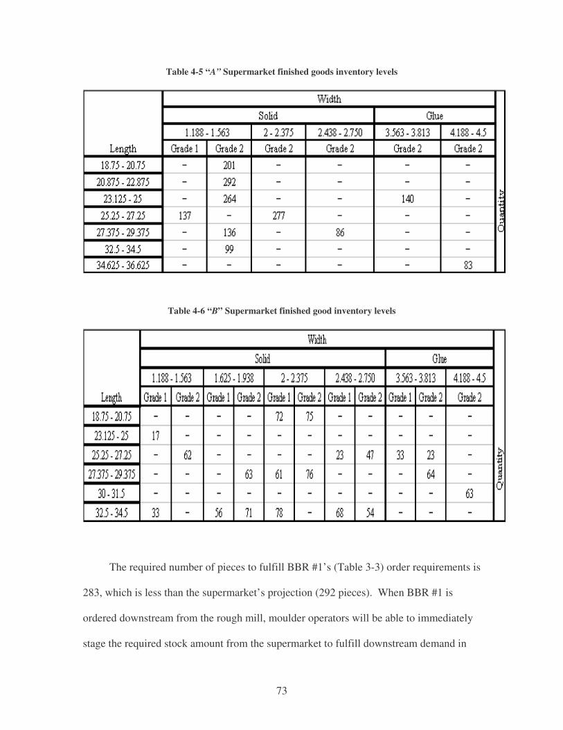
73

Table 4-5 “A” Supermarket finished goods inventory levels

Table 4-6 “B” Supermarket finished good inventory levels

The required number of pieces to fulfill BBR #1’s (Table 3-3) order requirements is

283, which is less than the supermarket’s projection (292 pieces). When BBR #1 is

ordered downstream from the rough mill, moulder operators will be able to immediately

stage the required stock amount from the supermarket to fulfill downstream demand in

74

essentially 19.8 minutes (lead time to mould). If the supermarket was not in place, this

order would have to be either scheduled in with the next 2-C poplar cutting or expedited

through the rough mill. The supermarket prevents overproduction by producing to actual

demand by maintaining replenishment standards. During the next time the rough mill

schedules 2-C yellow poplar the gang-rip/chop operation will replenish exactly what is

consumed.

4.5 Yield Simulation Since yield is currently the most important performance measure that is used

industry wide (Cumbo et al. 2006), testing the effects of cutting for solid parts on yield in

the second future state value stream was critical in determining the full impact of the

proposed changes. Currently, yield measurements at the study site are reported to

management daily via Barr-Mullins report. The yield report provides information solely

on overall yield and does not provide information on individual parts obtained during the

cutting that fulfill the current state value stream precisely. To get an unbiased difference

of yield, simulation is needed. ROMI-3 (Weiss and Thomas 2005), a rough mill

simulation software package described in Chapter 2.3.5 was used to simulate the yield of

the rough mill under study.

4.5.1 Current State ROMI-3 Settings

All information used to set-up the ROMI-3 (Weiss and Thomas 2005) simulation

was based on input from rough mill management and the company’s industrial

engineering department to best reflect the current state lumber cut up procedure at the

study site. Following ROMI-3 configuration settings, the rip saw setting selected was

75

Fixed-Blade-Best-Feed; the arbor spacing for all 4/4’’ poplar cuttings is shown in Table

3-6. As previously mentioned, the arbor spacing for 4/4’’ poplar is assumed not to

change between cuttings, this standard arbor configuration has been predetermined by

management and is assumed to maximize yield and limit changeover for all 4/4’’ poplar

cuttings. Additional information concerning gang-rip saw and chop-saw inputs is shown

in Table 4-7 and Table 4-8.

Table 4-7 Rip-saw inputs

Gang-Rip Inputs Current Arbor Width 22 1/16'' Saw Spacing Count 10 Ripsaw Kerf Size 3/16'' Left Edging Kerf 3/16'' Right Edging Kerf 3/16''

Table 4-8 Chop-saw Inputs

Chop-saw Inputs Endtrim allowance for each end 4/16'' Chop-saw Kerf size 3/16''

Table 4-9 represents inputs for the mill control feature. The term “salvage”

indicates parts require re-ripping to fulfill cutting bill requirements. Salvage parts in the

current system are obtained using “primary” lengths and widths; primary lengths and

widths represent part dimensions found in the cutting bill (Table 4-10).

76

Table 4-9 Mill control

Mill Control Processing units are in inches Part priorities are updated constantly Primary operations avoid orphan parts Salvage cuts to cutting bill requirements Random width strip parts okay in panels Minimum random width for panel parts = 1 1/4'' Maximum random width for panel parts = 2 3/4'' Board cutup optimization step = 4/16''

Table 4-10 Salvage Parts Inputs

Salvage Parts

Salvage uses primary widths Salvage uses primary lengths

Part prioritization was best defined in the simulation by the Complex Dynamic

Exponent (CDE) feature available; based on study site findings in Chapter 3.8.2. CDE is

a dynamic method of varying the priority emphasis placed on parts to be produced. CDE

allows part emphasis to change priority from one part to another as part quantities are

fulfilled (Weiss and Thomas 2005).

There are two part grades at the study site for internal nightstand components:

Part Grade 1 and Part Grade 2 (Table 4-11). Part Grade 1 requires both faces of the part

to be clear and free of defects (C2F). Part Grade 2 allows for sound knots and sap stain

and mineral streak.

Table 4-11 Part Grade parameters

Part Grades Grade Defect allowable Side

1 Clear, No defect Both Faces 1. Sound knots ‹ = .50 inch area Both Faces

2 2. Sap stain/mineral streak Both Faces

77

4.5.2 Future State ROMI-3 Settings

The majority of Future State ROMI-3 settings were assumed to not change: Arbor

spacing (Table 3-6), Rip-Saw Inputs (Table 4-7), Chop Saw Inputs (Table 4-8), Salvage

Parts Inputs (Table 4-10) and Part Grade Parameters (Table 4-11) all remained

unchanged. The only differences between the current and future state ROMI-3 (Weiss

and Thomas 2005) settings are:

• Modifications to the cutting bill (discussed in Section 4.5.4)

• Salvage cuts no longer fulfill cutting bill requirements

In order for salvage cuts to not fulfill cutting bill requirements, “Salvage cuts to

cutting bill requirements” feature has been turned off in the “Mill Control” (Table 4-9)

inputs. Salvage parts are the result of re-ripping and the future state’s goal is to produce

the correct dimensioned part from the gang-rip and chop operations without re-ripping

salvage. The yield difference between Current State and Future State ROMI-3 settings is

assumed to be representative of real differences.

4.5.3 Lumber Input

Using “The Databank for Kiln-Dried Red Oak” (Gatchell et al. 1998) within

ROMI-3, lumber used for the simulation was created based on an actual lumber load

input into the study rough mill. 2-C is the predominate grade when cutting 4/4’’ yellow

poplar. At the study site, lumber is only graded as green upon receiving and the actual

dried grade prior to lumber cutup is unknown. Table 4-12 is approximately the green

grade distribution of an 8748 BF 2-C yellow poplar cutting. Management felt this grade

distribution was representative of 2-C lumber inputs. Board lengths were made available

(Table 4-13) however width distribution were not available; therefore no minimum or

78

maximum board width was input into the system and boards of random width were

selected by the program. Fifteen different lumber files were created using for simulation

based on the information shown in Table 4-12 and Table 4-13.

Table 4-12 BF Grade Distribution

BF Grade Distribution

Grade BF % 1C 437.4 5 2C 7873.2 90 3C 437.4 5

Total 8748 100

Table 4-13 Board Length Distribution

Board Length Minimum Length 78'' Maximum Length 102''

4.5.4 Cutting Bills

Cutting Bill #1 (Appendix 3) is an example of an actual cutting bill used at the

study site and the cutting bill used to simulate the Current State value stream yield and

Future State value stream map #1. The cutting bill (Bill #1) for these value streams does

not change since panels are being produced. Again, the Current and Future State Value

stream map #1 assumes internal components will be glued in panels for multi-ripping.

Due to ROMI-3 restrictions on the amount of varying lengths and widths,

adjustments to the bill had to be made. The original cutting bill had more varying lengths

and widths than the software was capable of handling. To accommodate for software

limitations, parts whose lengths and widths were within 7/8’’in dimension in both length

and width were grouped together based on the greatest dimension (Table 4-14). Bill #1

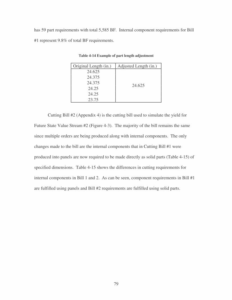
79

has 59 part requirements with total 5,585 BF. Internal component requirements for Bill

#1 represent 9.8% of total BF requirements.

Table 4-14 Example of part length adjustment

Original Length (in.) Adjusted Length (in.)

24.625 24.375 24.375 24.25 24.25 23.75

24.625

Cutting Bill #2 (Appendix 4) is the cutting bill used to simulate the yield for

Future State Value Stream #2 (Figure 4-3). The majority of the bill remains the same

since multiple orders are being produced along with internal components. The only

changes made to the bill are the internal components that in Cutting Bill #1 were

produced into panels are now required to be made directly as solid parts (Table 4-15) of

specified dimensions. Table 4-15 shows the differences in cutting requirements for

internal components in Bill 1 and 2. As can be seen, component requirements in Bill #1

are fulfilled using panels and Bill #2 requirements are fulfilled using solid parts.

80

Table 4-15 Internal nightstand components in Bill #1 and Bill #2

Bill # Width Length Quantity Grade

Panel (1=panel, 0=solid)

1 14.875 34.625 19 2 1 2 1.375 34.625 187 2 0 1 22.875 24.625 17 2 1 2 2 24.625 168 2 0 1 21.625 21.5 66 1 1 2 2.375 21.5 528 1 0 1 23.75 24.625 17 2 1 2 2 24.625 168 2 0 1 14.875 24.625 52 2 1 2 1.375 24.625 338 2 0 2 2 24.625 169 2 0

Due to the current state system which features a fixed blade best feed system

gang-rip saw, not all internal components could be successfully obtained in the correct

dimension. The arbor sizes did not exactly fit components required widths therefore part

sizes were increased to the closest arbor width of a greater size. For example, if an

internal component final part width requirement was designed to be 1.25’’; in Bill #2 the

part width was adjusted to 1.375’’ (closest arbor width of greater size). This resulted in a

total yield loss of 28 BF in the cutting and was accounted for in simulated yield results

found in Table 4-16. This loss would occur during the moulding operation of the

product. Future studies would require the determination of an optimum arbor spacing

design should Future State #2 be adopted, this would perhaps improve yield.

81

4.5.5 Panel Production

According to Weiss and Thomas (2005) a panel is defined as “a panel or glue-up

part is made of two or more solid parts that have been edge glued together”. ROMI-3

simulates panel production by cutting for: 1.) Solid parts of specified length and 2.) Solid

parts of either specified or random width. The user is given the option to cut for specified

or random width. This option is found in the Mill Control feature under the option

“Random width strip parts okay in panels”.

Random width is generally selected when a movable blade arbor is present when

no specified part widths are present and parts are of “true” random width. Even though

“true” random width parts are not obtained at the study site because the arbor is fixed

blade, the “Random width strip parts okay in panels (Table 4-9)” was still enabled. This

feature was enabled because no specific solid part width for panels is defined at the mill

and any of the solid part widths can be used at random to create panels, thus creating

random width part panel production.

4.5.6 Methods

Yield in ROMI-3 is broken down into 4 categories: 1.) Primary, 2.) Salvage, 3.)

Excess salvage and 4.) Total. Primary indicates yield that is obtained to fulfill cutting

bill requirements. Salvage yield is the result is re-ripping to fulfill cutting bill

requirements as mentioned previously. Excess Salvage is yielded parts that do not fulfill

cutting bill requirements and require storage until a need is found for that particular part.

Total yield is the summation of primary, salvage and excess salvage.

Using ROMI-3, 30 simulations were made to determine whether a difference in

yield existed when the gang-rip cut parts for glue up (Current and Future state #1) or for

82

solid parts (Future State #2). The cutting bill for the Current and Future state #1 (Bill 1;

Appendix 3) was replicated 15 times and the cutting bill for Future State #2 (Bill 2;

Appendix 4) was also replicated 15 times. Since 15 yield results from the manufacturer

were obtained (Control), each simulation was replicated 15 times.

The overall yield obtained from the ROMI-3 simulations was the measurement

used to define the Current and Future State #1 yield. Primary, Salvage and Excess

Salvage are all included in the yield measurement of the study site. Overall yield best

reflects the manner which yield is determined at the study site.

The primary yield was the measurement used to define the yield for Future State

#2. Because Future State #2 calls for the elimination of non-value added activities, the

salvage yield was not applied in the simulations (Chapter 4.5.2). One limitation of

ROMI-3 (Weiss and Thomas 2005) was the programs inability to turn off excess salvage

production (unusable parts); therefore the overall yield differed from the primary yield.

The primary yield measurement was separated from the overall yield measurement.

Using the Statistical Analysis System Institute SAS (1988) software, the

following yield results were compared for differences among means:

1. Null Hypothesis = Overall yield of Control and Bill #1 will be the same.

Research Hypothesis = Overall yield of Control and Bill #1 will be different.

2. Null Hypothesis = Overall yield of Bill #1 and Bill #2 will be the same.

Research Hypothesis = Overall yield of Bill #1 and Bill #2 will be different.

3. Null Hypothesis = Overall yield of Bill #1 and Primary yield of Bill #2 will be

the same.

83

Research Hypothesis = Overall yield of Bill #1 and Primary yield of Bill #2

will be different.

Test #1 of overall yield of both the control (actual study site reporting) and

Cutting Bill #1 (Current and Future State #1) will determine whether ROMI-3 simulation

is an acceptable program for use in assessing possible yield differences in Cutting Bill #1

(Current and Future State #1) and Cutting Bill #2 (Future State #2). Test #2 was

performed to determine whether overall yield differs between Cutting Bill 1 and 2. Test

#3 will determine whether a difference in yield exists between the Overall yield of Bill #1

(Current and Future State #1) and the Primary of Bill #2 (Future State #2).

4.5.6.1 Results Two sample t-tests were used to compare means of actual (control) and simulated

results (SAS 1988; Proc TTest). Sample and actual samples were first tested for equality

of variances using the Folded Form F Statistic. If variances were statistically found not

to be equal, the Cochran and Cox Approximation (SAS 1988) of the approximate t

statistic was used. Otherwise, the t test for independent samples with pooled variances

was used. All tests were considered significant at P < 0.05.

Table 4-16 T-test results and statistics of actual and simulated yield models

Test # Comparison Mean SE Folded F Test T-Test Control 57.75 0.49 P < 0.001 P < 0.001 1

Bill #1 54.52 0.06

Overall Bill #1 54.52 0.06 P = 0.61 P < 0.001 2 Overall Bill #2 55.43 0.05

Overall Bill #1 54.52 0.06 P = 0.51 P < 0.001 3 Primary Bill #2 53.01 0.05

84

4.5.6.2 Discussion

Thomas and Buehlmann (2002) validated ROMI-RIP (Thomas 1996) (original

simulation of ROMI-3) and found simulated yields were significantly higher (7%) than

actual rough mill yield. This contradicts findings shown in Table 4-16 which found that

simulation results to be lower than actual results (Test #1); however, in the authors study

(Thomas and Buehlmann 2002) all part requirements were solid and not glued panels.

Part dimension adjustment due to software limitations (Table 4-14) may have also

contributed to a decrease in yield. However, it was previously mentioned (Chapter 4.4.1)

that parts often exit the rough mill with greater dimension indicating that part dimension

adjustment in the simulation may not have affected yield.

Currently, no validation study of ROMI-RIP has been performed using panel parts

as cutting bill requirements therefore it is unknown whether Thomas and Buehlmann’s

(2002)’s findings apply to panel part production. As solid parts requirements increase in

Bill #2 from Bill #1 (Test #2), so does the overall yield (Table 4-16). This may support

Thomas and Buehlmann’s (2002) validation study findings that ROMI-RIP outperforms

rough mill yield when producing solid parts and also suggests that ROMI-RIP may

underperform when producing panel parts as compared to actual rough mills. At this

point in time it can only be assumed that ROMI-3 is sufficiently valid for relative

comparison of cutting bills. Therefore, results found in Table 4-16 were considered

applicable for this study’s purposes of assessing potential yield differences that exist for

Future State #2.

In Test #3 the Primary yield of Bill #2 (determined yield measurement of Future

State value stream #2) differs from the Overall yield of Bill #1 (determined yield

85

measurement of Current State and Future State value stream #1). This can be explained

by Salvage and Excess salvage yield that remained in the ROMI-3 simulations of Bill #1.

The average effect of yield loss (1.51%) in Bill #2 will be used as the basis of comparison

in the financial analysis of Chapter 5.

4.6 Lead Time

By eliminating inappropriate processing the lead time of Future State #2 (7.5 hours)

is reduced by more than half of the Current and Future State #1 (15.1 hours). It should be

noted that lead time for all value streams, current and future is relative to once 2-C

yellow poplar is scheduled to run through the rough mill. The addition of part

supermarkets in both future state value streams allows for immediate response to actual

demand downstream. With the implementation of a part supermarket, all lead and value

added operations upstream from the supermarket have already been performed based on

previous actual part demand. This differs from the Current State where operations are

performed based on a forecast of demand. If demand changes in the Current State, all

processing steps must be performed starting at the rough planer. In both future states, as

long as the supermarket has the specified inventory levels, only the moulding operation is

required to meet an immediate change in demand.

4.7 On-Time Delivery

To obtain an accurate representation of on-time delivery the supermarkets must

physically be in place and as of the time of this study supermarkets were not present at

the study site. Although on-time delivery is a measure that can not be defined in this

study it is believed that the supermarkets would only increase the percentage of parts

86

exiting the rough mill. Supermarkets provide safety in the system by maintaining

predetermined demanded inventory levels which buffer against possible machine

breakdown and order expediting. Decreased lead time in Future State Value Stream #2

(Chapter 4.6) allows for increased probability of meeting downstream demand in a more

timely manner.

4.8 Improvement Opportunities

As mentioned in Chapter 3.12 opportunities exist at the study site for improvement

in the areas of: overproduction, unnecessary inventory, waiting, inappropriate processing,

defects, transportation and motion. Based on the findings of Chapter 3.12 in these areas

the following opportunities exist based on the implementations of the proposed

supermarket pull system.

4.8.1 Overproduction

Multiple point scheduling and forecasting in the Current State was determined to

be the reason for overproduction. Since overproduction has been determined to be the

root cause of all manufacturing waste, it was essential to focus on this area in both Future

State value streams. To reduce overproduction, production scheduling has been reduced

to 1 point; at the supermarket. Scheduling at the supermarket means production is based

on actual downstream demand, and not to a forecast. Production in forecasting results in

the production of parts that are not in current demand. This 1 point schedule based on

actual demand results in the reduction of all other waste opportunities found in the

Current State evaluation (Rother and Shook 2003).

87

4.8.2 Unnecessary Inventory

Unnecessary inventory in the Current State has been replaced with necessary

supermarket inventory that maximizes production effectiveness in meeting demand.

Overproduction and multiple point scheduling resulted in unnecessary inventory in the

Current State. By producing to supermarket requirements in both Future States, all

inventories are standardized in that it provides a buffer to best deal with current system

uncertainties. Through scheduling production at 1 point based on demand, inventory will

not be produced until demanded, which is the goal of the rough mill

4.8.3 Waiting

It was found that waiting at the study site was the result of machine changeover

and operators locating orders. The purpose of this study was not to decrease machine

changeover time as currently the manufacturer is undergoing this practice. With the

supermarket, all orders for the moulding operation are kept in one location and no

searching is necessary. Searching for orders upstream from the supermarket in Future

State Value Stream #1 (Figure 4-2) should decrease with the implementation of FIFO

lanes. The FIFO lanes, if properly designed will keep order in the system. In Future

State Value Stream #2 (Figure 4-3), inappropriate operations have been removed

therefore searching for orders has virtually been eliminated.

4.8.4 Inappropriate Processing

Two processes were found to be non-value added in the Current State; edge-

gluing and multi-ripping. While these activities remained in Future State #1 as necessary

operations, they were eliminated in Future State #2 for parts that fit within the standard

88

gang-rip arbor set-up. Additional processing results in increased labor and overhead

costs and limits the flexibility of the system to meet demand. The lead time was reduced

to more than half of the Current and Future State #1 by removing these processes in

Future State #2.

4.8.5 Defects

Defects in the Current State evaluation were observed in overages and shortages.

Overages in the current state exist due in part to the spoilage factor applied by the MRP

scheduling system. If the overage applied to an order as seen in Table 3-9 is too great (no

parts are spoiled), these excess parts are essentially thrown away. With the addition of

the supermarket, only the correct amount of parts is withdrawn from the supermarket

eliminating the possibility of wasting excess product when the order leaves the rough

mill. By decreasing overages in the system, time wasted machining excess parts has been

reduced if not eliminated. Excess parts which exist from operations upstream from the

supermarket are maintained as part of the supermarkets inventory.

Shortages led to expediting parts through the Current State Value Stream (Chapter

3). Expediting parts is a confusing and cumbersome undertaking when many different

parts are being produced simultaneously. It is critical when expediting to make sure not

only the expediting parts are manufactured but also the current schedule is maintained.

If a part shortage occurs currently, the entirety of the rough mill manufacturing

procedure must be undergone. With the addition of the supermarket, all rough mill

procedures other than the moulding operation have already been undergone eliminating

unnecessary manufacturing. In essence, the supermarkets in both Future State’s create an

organized systematic way to avoid expediting. If moulder bites or other machining

89

defects occur at the moulding operation, additional product can be withdrawn as needed

from the supermarket. The safety factors (buffer and safety stock) built into the

supermarket are in place to cover overage occurrences.

4.8.6 Transportation

Internal components will remain on the previously discussed carts (Chapter

3.12.6) for transportation throughout the rough mill before entering the supermarkets. In

Future State #1, cart usage will remain an issue however Future State #2 cart usage is

reduced significantly with the elimination of inappropriate processing activities. Parts in

Future State #2 will travel straight from the chop operation to the supermarket. The

supermarket provides a central inventory holding location and will decrease the number

of occupied carts that workers must sort through when finding orders to process at other

operations.

4.8.7 Motion

With the reduction or elimination of previously mentioned shortages and

overages, waste in unnecessary production motion has been reduced. Although Future

State #1 maintains non-value added activities, Future State #2 has eliminated non–value

added activities and reduced unnecessary motion. The supermarket provides a central

location for internal nightstand components which reduces the amount of motion

currently spent on locating orders to process. Production in both Future State’s is based

on actual demand, unlike the Current State where production is based on a forecast.

When production in based on a forecast, all motion (value added and non-value added

activities) is wasted if the forecast is inaccurate.

90

5 Value Stream Evaluations for Cost Effectiveness

The purpose of this chapter was to evaluate the cost feasibility of all rough mill value

stream maps discussed (Current State, Future State #1 and Future State #2). Figure 5-1

displays the rough mill costs as compared to all costs at the study site. As can be seen,

rough mill costs rank third of all manufacturing processes.

The following information was used for this evaluation: 1.) Labor, 2.) Overhead and

3.) Lumber Costs. This information was provided by the manufacturer and figures have

been adjusted to maintain confidentiality. This evaluation will determine whether the

Future state value stream maps (Figure 4-2; Figure 4-3) proposed in Chapter 4 are

economically viable as compared to the Current State value stream map (Figure 3-5)

when producing the sample internal component order BBR #1 (Table 3-3).

Furniture M anufacturing C osts

M ateria l Co s ts45%

W areh o u s e/ Sh ip p in g

3% Fin is h6%

A s s emb ly11%

Packin g4%

M ach in in g & San d in g

14%

Ro u g h M ill7%

M arg in /Pro fit10%

Figure 5-1 Furniture manufacturing costs (provided by study site)

91

5.1 Methods

To determine the cost effectiveness the following information was used to

determine the Total Cost to manufacture order BBR#1 (Table 3-3): Lumber, Labor and

Overhead costs. The summation of Lumber, Labor, and Overhead cost per value stream

determined the Total Cost of each value stream. Labor and overhead are shown for each

machining operation. This information was based on the information provided by the

manufacturer.

The yield metric is the driving metric at the rough mill under study and it is

hypothesized that an emphasis to focus on reducing material costs increases labor and

overhead costs. The yield simulation results found in Objective #2 were used to

determine whether a decrease in the yield measurement due to the removal of the panel

glue-up operation in Future State #2 outweighs the processing costs.

5.2 Current State Value Stream

In the Current State Value Stream (Chapter 3) the following processes were

considered in the cost analysis: Rough Planer, Gang-Rip, Chop Saw, High Frequency

Gluing, Multi-Ripping and Moulding. While the actual rough mill yield obtained from

the study site was found to be 57.74% (Figure 3-6), the overall yield of 54.52% (Table

4-16) obtained from ROMI-3 (Weiss and Thomas 2005) was used in the financial

analysis to maintain a repeatable standard yield basis to compare all Future State cases.

Even though a statistical difference exist between the actual (Control) and ROMI-3 (Bill

1) results (Chapter 4.5.6.2), the ROMI-3 measurement will allow for an applicable cost

comparison in the Future State Value Stream Map #2 analysis (Chapter 5.4) where yield

92

measurements were obtained using ROMI-3 simulations. A lumber input cost of

$300/MBF or $0.30/BF for 2-C yellow poplar remained constant throughout the analysis.

5.2.1 Lumber, Processing and Total Costs

Table 5-1 represents the lumber costs for the current state value stream based on

the finished BF requirement of 60 (Table 3-3). Table 5-2 through Table 5-5 represent the

processing costs for the operations found in the Current State Value Stream Evaluation

(Chapter 3) to produce order BBR#1. 110.05 BF (Table 5-1) and 495 LF (Table 3-3) was

used in determining operating costs. The total costs to produce order BBR#1 are

displayed in Table 5-6 and Figure 5-2.

Table 5-1 Current State Value Stream Lumber Costs for order BBR#1

Lumber Costs

Finished BF Required 60 Yield 54.52

Rough BF Required 110.05 Cost Per BF $0.30

Total Lumber Cost $33.02

Table 5-2 Rough Planer/Gang-Rip/Chop-saw costs

Rough Planer/Gang-Rip/Chop Saw

Total labor required 17 Average wage $10.92 Labor Cost/hr. $185.64

Variable OH Costs/hr. $154.41

4/4 2-C Poplar BF/hr. 2000

Operating Costs per BF $0.17 110.05 BF Operating Costs $18.71

93

Table 5-3 High-frequency gluing operation processing costs

High Frequency Gluer Total labor required 6

Average wage $11.36 Labor Cost/hr. $68.16

Variable OH Costs/hr. $47.43 4/4 2-C Poplar BF/hr. 1000

Operating Costs per BF $0.12 60 BF Operating Costs $6.94

Table 5-4 Multi-Rip operating costs

Multi-Rip Total labor required 2.5

Average wage $11.36 Labor Cost/hr. $28.40

Variable OH Costs/hr. $23.71 4/4 2-C Poplar BF/hr. 750

Operating Costs per BF $0.07 60 BF Operating Costs $4.17

Table 5-5 Moulder costs

Moulder (1 of 8)

Total labor required 2.375 Average wage $11.80 Labor Cost/hr. $28.03

Variable OH Costs/hr. $28.22 4/4 2-C Poplar LF/hr. 1500

Operating Costs per LF $0.04 495 LF Operating Costs $18.56

94

Table 5-6 Total Cost of Current State value stream to produce order BBR #1

Total Processing Cost 2-C Yellow Poplar BF Costs $33.02

Rough Planer/Gang-Rip/Chop Saw $18.71 High Frequency Gluer $6.94

Multi-Rip $4.17 Moulder (1 of 8) $18.56

Total Cost To Produce Order BBR #1 $81.39

Current Sta te V alue Stream Tota l Costs to produce order BBR# 1

M o ulder (1 o f 8 ) $ 1 8 .5 6

M ult i-Rip $ 4 .1 7

H igh Frequen cy Gluer $ 6 .9 4

Ro ugh P lan erGan g-RipCh o p Saw $ 1 8 .7 1

2 -C Y ello w P o p lar BF Co st s

$ 3 3 .0 2

Figure 5-2 Total Cost of Current State Value Stream to produce order BBR #1

5.3 Future State Value Stream #1

Future State Value Stream Map #1 (Figure 4-2) processing and cutting bill

(Appendix 3) does not differ from the Current State Value Stream therefore direct

material, labor and processing costs do not differ. The only difference between the

Current and Future State #1 is the implementation of a part supermarket in Future State

95

#1. While processing improvements currently exist in the Current State system that could

possibly reduce operating costs, testing these improvements were outside of the scope of

this project therefore all operations and costs remain the same.

5.4 Future State Value Stream #2

The following processes were considered in the cost analysis in Future State Value

Stream #2: Rough Planer, Gang-Rip, Chop Saw and Moulding. Future State Value

Stream #2 was designed to reduce inappropriate processing that may prevent the rough

mill from meeting downstream demand. Therefore, non-value added processes (gluing or

multi-ripping) and their respective costs were eliminated. To eliminate these activities,

internal components were obtained as solid parts in Cutting Bill #2 (Appendix 4) from

the Gang-Rip and Chop operation as opposed to panel parts in Cutting Bill #1 (Appendix

3; Current State and Future State 1).

The primary yield measurement (53.01%; Table 4-16) from Bill #2 ROMI-3

simulation was used in the evaluation. The primary yield, not overall yield, was selected

for evaluation because overall yield includes salvage yield which is the result of

inappropriate processing (Chapter 4.5.6). Reducing waste such as inappropriate

processing is the goal of Future State #2.

5.4.1 Lumber, Processing and Total Costs

Table 5-1 represents the lumber costs for the current state value stream based on a

finished requirement of 60 BF (Table 3-3). 113.19 BF (Table 5-7) and 495 LF (Table

3-3) was used in determining operating costs (Table 5-8). Table 5-8 represents the

operating costs Future State Value Stream #2 (Figure 4-3) to produce order BBR#1; the

96

moulding costs shown in Table 5-5 does not change therefore this cost is only shown in

the Total Costs (Table 5-9).

Table 5-7 Future State Value Stream Map #2 Lumber Costs

Lumber Costs

Finished BF Required 60 Yield 53.01

Rough BF Required 113.19 Cost Per BF $0.30

Total Lumber Cost $33.96

Table 5-8 Rough Planer/Gang-Rip/Chop-saw Costs

Rough Planer/Gang-Rip/Chop Saw Total labor required 17

Average wage $10.92 Labor Cost/hr. $185.64

Variable OH Costs/hr. $154.41

4/4 2-C Poplar BF/hr. 2000

Operating Costs per BF $0.17 113.19 BF Operating Costs $19.24

Table 5-9 Total Cost of Future State Value Stream #2 to produce order BBR #1

Total Processing Cost 2-C Yellow Poplar BF Costs $33.96

Rough Planer/Gang-Rip/Chop Saw $19.24 Moulder (1 of 8) $18.56

Total Cost To Produce Order BBR #1 $71.76

97

F uture Stat e Value St ream M ap #2 T otal Cost s to p roduce order BB R#1

M o ulder (1 o f 8 ) $ 1 8 .5 6 2 -C Y ello w

P o p lar BF Co st s $ 3 3 .9 6

Ro ugh P lan erGan g-RipCh o p Saw $ 1 9 .2 4

Figure 5-3 Total Cost of Future State Value Stream #2 to produce order BBR #1

Figure 5-4 displays the operating costs by machine work center. As can be seen,

Future State #2 lumber input and Rough Planer/Gang-Rip/Chop Saw costs were higher

than Current and Future State #1. More lumber and machine processing is needed to

fulfill Future State #2 needs due to the yield simulation results found in Chapter 4.5.6.1.

While these costs are higher in Future State #2, they do not outweigh the costs to edge-

glue and multi-rip found in the Current and Future State #1. The costs associated with

the yield difference in Future State #2 were minimal compared to the costs associated

with edge-gluing and multi-ripping. This shows that a focus on the yield metric does not

always guarantee a cost effective system.

98

C ost Breakdown

$ 6 .9 4

$ 4 .1 7

$ 1 8 .5 6

$ 3 3 .0 2

$ 1 8 .7 1

$ 3 3 .9 6

$ 1 9 .2 4

$ -

$ 5 .0 0

$ 1 0 .0 0

$ 1 5 .0 0

$ 2 0 .0 0

$ 2 5 .0 0

$ 3 0 .0 0

$ 3 5 .0 0

$ 4 0 .0 0

L um ber co st s Ro ugh P lan er, Gan g-Rip ,

Ch o p Saw

H igh Frequen cyGluer

M ult i-Rip M o ulder

M ach in in g Pro ces s

Cos

t Curren t St at e an dFut ure St at e # 1

Fut ure St at e # 2

Figure 5-4 Total Cost breakdown

5.5 Break Even Point

Even though Bill #1 (Appendix 3; Current and Future State #1) produced a higher

yield than Bill #2 (Appendix 4; Future State #2), Future State #2 total costs ($71.76)

(Table 5-9) was found to be less than the Current and Future State #1 (Table 5-6). The

elimination of non-value added activities (gluing and re-ripping) outweighed the costs of

yield loss. The primary yield measurement would have to drop to 44.89% or below in

Future State Value Stream #2 before a monetary loss in experienced.

Table 5-10 Yield Adjustments to Determine Break Even Point

Future State Value Stream #2 Break Even Analysis

Yield (%) 53.01 51 49 47 45 44.89 Yield loss (%) � 2.01 4.01 6.01 8.01 8.12

Monetary difference $71.76 $73.86 $76.12 $78.57 $81.23 $81.39

99

$64.00$66.00$68.00$70.00$72.00$74.00$76.00$78.00$80.00$82.00$84.00$86.00

0 � 2 � 4 � 6 � 8 � 10

Yield % Loss

Cos

t

FutureSta te # 2

CurrentandFutureSta te # 1

Figure 5-5 Break even yield measure

5.6 Total Cost Saving Potential

Table 5-11 displays the total cost to produce the 109,858 internal nightstand

components in 2006 assuming all internal components have the same physical

characteristics as order BBR #1 (Table 3-3). Even though this is will not be the case as

each finished nightstand is different in style, Table 5-11 does represent savings potential.

As gluing increases from 100% solid (Future State #2) to 100% glued (Current and

Future State #1), so does the yearly costs. Not only is Future State #2 a more cost

effective way to meet downstream demand but it also is a more cost effective way to

manufacture internal nightstand components.

Table 5-11 Yearly costs to produce internal nightstand components

100% Solid 70% Solid, 30% Glue

70% Glue, 30% Solid 100%Glue

$27,856.57 $ 28,978.06 $ 30,473.37 $31,594.85

100

Figure 5-6 represents the total yearly costs to manufacture all internal

components, not solely nightstand components. Similar to the findings in Table 5-11, as

gluing increases so does the total costs to manufacture these components. While not all

internal components can be obtained as solid parts due to part dimension requirements

and gang-rip operation arbor limitations, Figure 5-6 represents the potential yearly

savings by reducing edge-glued panel production.

All Internal C omponents

$523,791.23

$544,878.65

$594,082.61

$572,995.20

$480,000

$500,000

$520,000

$540,000

$560,000

$580,000

$600,000

100% Solid 70% Solid, 30% Glue

70% Glue, 30% Solid

100% Glue

Cos

t $

Figure 5-6 All Internal Components Yearly Costs

101

6 Conclusions

The major advantages for domestic furniture manufacturers are proximity to the final

customer and ability to meet demand customer due to decreased lead times. Lower labor

costs available in foreign countries have pushed many organizations towards the import

market thus widening the gap between proximity and customer demand. Opportunity

exists for domestic secondary manufacturers by increasing their ability to meet customer

demand.

The Rough Mill is the first step in furniture manufacturing and carries the

responsibility of meeting downstream demand of all furniture operations. Traditionally,

the rough mill has been a push based yield driven system. Because lumber represents a

significant cost, non-value added yield recovery activities such as edge-gluing and

salvage operations have been put into place in rough mills. While these activities are

necessary when solid parts are unobtainable by the gang-rip arbor type due to dimension

requirements, they only increase lead times and manufacturing costs of obtainable solid

parts. The push based system coupled with non-value added activities limits the rough

mill’s ability to meet downstream demand changes in not only the furniture plant but

ultimately to the final customer.

One manufacturing method proven in other industries to successfully respond to

customer demand is “pull” manufacturing. In a pull system, production is not based on a

forecast like so many manufacturers have relied upon; it is based on actual demand. By

producing to demand, overproduction and inappropriate processing does not tie up rough

mill production with undemanded products which will eventually lead to finished good

inventory. Lead times can be reduced significantly by maintaining small amounts of

102

known demanded inventory in the manufacturing process in “supermarkets”. Because

the rough mill is the first manufacturing process, the success of the furniture operation to

meet final customer demand weighs heavily on this process. The reduction of lead time

in the rough mill ultimately reduces the furniture operations overall lead time to the

customer, increasing the competitive advantage it maintains against foreign competitors.

The domestic cabinet industry has found success using such techniques. On-time

delivery to downstream demand has increased through the reduction of lead times and

manufacturing waste. The cabinet industry has proven these techniques are applicable to

the wood products industry and this opportunity exists for all wood products

manufacturers (Merillat 2003; Ray et al. 2006).

This project demonstrates how manufacturing techniques such as pull systems and

value stream mapping can be applicable to the rough mill. These techniques have proven

that manufacturing steps that are currently in place to salvage yield result in increased

lead time and cost. While this project focused on only one of many products at one study

site, its findings are applicable for any manufacturer of dimension lumber pieces.

6.1 Research Objectives Findings

The purpose of this research was to provide a method for rough mill systems to

become more competitive by decreasing lead time to meet downstream demand. The

objectives of this research project were:

1) To perform a current state value stream evaluation of the rough mill

manufacturing system.

2) To design an improved rough mill future state value stream that is responsive to

downstream demand using pull system methodologies.

103

3) To demonstrate the cost effectiveness of the future state value stream using a

furniture manufacturing case study.

6.1.1 Objective 1

The first objective concerned a current state value stream evaluation of the rough

mill manufacturing system at a furniture company located in Virginia. The evaluation

focused on the manufacturing processing currently in place to produce internal nightstand

components, specifically order BBR#1 (Table 3-3). The information used to create this

value stream was based on on-site investigation and input from management and shop

floor employees.

The current state evaluation found that production scheduling for the rough mill

was performed based on forecasting using an MRP system. Lead time was determined to

be 907.2 minutes (15.1 hours) while value-added time was 31.5 minutes. Two activities

were determined to be non-value added (high-frequency edge gluing and multi-ripping).

On-time delivery from the rough mill to downstream processes was highly variable and

ranged from 53% to 96%. Overproduction was determined to be the root cause of the

rough mill’s inability to meet downstream demand. Overproduction was caused by

forecasted production and multiple point scheduling and resulted in products being

produced before they are in actual demand. To alleviate overproduction, production

should be based on actual demand and scheduled at 1 point.

6.1.2 Objective 2

The second objective involved the design of 2 value streams (Future State #1 and

Future State #2) using pull and supermarket system methodology. Future State #1 and #2

104

were developed based on the findings from the Current State evaluation (Objective #1).

Just as the Current State, both Future State value stream maps were developed using

example internal nightstand component order BBR#1 (Table 3-3). Production was

scheduled at 1 point in both Future States decreasing all waste associated with

overproduction.

Future State #1’s design was similar to the Current State evaluation in that all

machining processes remained (value added and non-value added). The overall lead time

of Future State #1 did not differ from the Current State (15.1 hours). However, the

implementation of a part supermarket allows the system to pull parts through the rough

mill to satisfy immediate customer demand in a more efficient manner.

Future State #2 is a simpler version of the Current State and Future State #1. The

only processes that were included in this design were value-added processes. Edge-

gluing and subsequent multi-ripping were removed to reduce inappropriate processing.

The overall lead time of Future State #2 was reduced by more than half (7.5 hours) and

the time to replenish the part supermarket was decreased as well, meaning the system is

more flexible to respond to downstream demand. However, Future State #2 produced a

lower yield measurement than the Current and Future State #1.

6.1.3 Objective 3

The third objective involved a cost evaluation of the Current State, Future State 1

and Future State 2 value stream evaluations performed in Chapter 3 and 4. The

information used to perform this analysis was: lumber, labor and overhead costs. Future

State #2 proved to be the most cost efficient value stream even though it produces the

lowest yield measurement. The elimination of inappropriate non-value added processes

105

outweighed the additional lumber costs required. Yield in Future State #2 would have to

be 8.12% lower than the Current and Future State #1 before Future State #2 would prove

to be not cost effective.

6.2 Future Research and Limitations

This project was limited to the boundary of the rough mill of a furniture

manufacturer. While this project may prove to be beneficial for the rough mill, the real

opportunity is beyond the rough mill. The cost of not meeting demand in the studied

operation was outside the scope of this project as all costs associated with backlog and

reschedules were unavailable. However, it is an area that future research should focus on

and should not be limited to just the rough mill.

The value stream was limited to internal nightstand components. This was

performed because the system is too complex to take on all value streams. The methods

used focus on all issues in-depth for one component; this approach is applicable for other

component value streams as well. Similar opportunities are hypothesized and require

future states.

Yield simulation was used in this project and can only be assumed to represent the

study rough mill. While simulation is a working research tool, it cannot simulate exactly

what a rough mill does. Sensitivity studies showed that yield would need to drop lower

than 8% over current yield before proposed changes would cause a negative cost impact.

The material used in this study (2-C yellow poplar) is a lesser valued species and this

would not be the case for higher value species but the relatively large margin indicates

potential for many other component value streams. Future research is needed to

understand this better.

106

Furniture part design currently exists without knowledge of how it affects

manufacturing procedures. Many similar part sizes exist for different part SKU’s, a

standard design system can be created to impact yield positively while maximizing part

flexibility for many different part value streams. While past research has been performed

which looks into solid parts and panel standardization (Araman and Lucas 1975; Araman

and Hansen 1983), future research should focus on the applicability of standard part

design for pull system implementation.

107

References Anonymous (N.D.). Waste Reduction Guide: Wood Furniture Industries. T. V. A.-.

Knoxville, Dolan-Friss Associates, Preventive Environmental Management, Radian Corporation.

Araman, P. and B. Hansen (1983). Conventional Processing of Standard-Size Edge-Glued Blanks for Furniture and Cabinet Parts: a Feasibility Study. U. S. D. o. Agriculture, Forest Service, Northeastern Research Station, Broomal. PA: 15.

Araman, P. and E. Lucas (1975). An Automated Rough Mill for the Production of Interior Furniture Parts. U. S. D. o. Agriculture, Forest Service, Northeastern Research Station, Upper Darby, PA: 5.

Bhoot, A. (2004). Development of an Order Promising Framework for Furniture Industry. Industrial Engineering, Mississippi State University. M.S. Thesis.

Brunner, C. C. (1984). CORY - A computer program to determine furniture cutting yields from both rip-first and crosscut-first sawing sequences. Wood Science and Forest Products. Blacksburg, VA, Virginia Tech. PhD Dissertation.

Buehlmann, U. (1998). Understanding the relationship of lumber yield and cutting bill requirements: a statistical approach. Department of Wood Science and Forest Products. Blacksburg, VA, Virginia Tech. PhD Dissertation.

Buehlmann, U., M. Bumgardner, A. Schuler and R. Christianson (2003). "US Competitiveness Study: How Furniture and Cabinet Manufacturers Compare." Wood and Wood Products 108(May): 49-51.

Bumgardner, M., U. Buehlmann, A. Schuler and R. Christianson (2004). "Domestic competitiveness in secondary wood industries." Forest Products Journal 54(10): 21-28.

Cao, X., E. N. Hansen, M. Xu and B. Xu (2004). "China's Furniture Industry Today." Forest Products Journal 54(11): 14-23.

108

Cumbo, D., D. E. Kline and M. Bumgardner (2006). "Benchmarking Performance Measurement and Lean Manufacturing in the Roughmill." Forest Products Journal 56(6): 25-30.

De Bodt, M. (1983). "Cost increases due to demand uncertainty in MRP lot sizing." Decision Science 14(3): 345-362.

Deleersnyder, J. L., T. J. Hodgson and P. J. O'Grady (1989). "Kanban Controlled Pull Systems: An Analytic Approach." Management Science 35(9): 1079-1091.

Gatchell, C. J. (1987). "Rethinking the design of the furniture rough mill." Forest Products Journal 31(3): 8-14.

Gatchell, C. J., E. Thomas and E. Walker (1998). 1988 Data Bank for kiln-dried red oak lumber. Gen. Tech. Rep. NE-245. N. R. S. Forest Service, U.S. Department of Agriculture: 60.

Giese, P. J. and J. D. Danielson (1983). CROMAX - a crosscut first computer simulation program to determine cutting yield. U. F. Service. Madison, Wisconsin, Forest Products Lab.

Hamner, P. C., B. H. Bond and J. K. Wiedenbeck (2002). "The effects of lumber lengths on part yields in gang-rip-first rough mills." Forest Products Journal 52(5): 71-76.

Ho, C. J. and T. C. Ireland (1993). "A diagnostic analysis of the impact of forecast errors on production planning via MRP system nervousness." Production Planning & Control 4(4): 311-322.

Kline, D. E., A. Widiyoko, J. K. Wiedenbeck and P. Araman (1998). "Performance of color camera-based machine vision system in automated furniture rough mill systems." Forest Products Journal 48(3): 38-45.

Langer, F. (2004). "The Fast Path to Excellence..Trimming the Fat Through Lean Manufacturing." abf journal 2(10).

Lee, T. S. and E. A. Everett (1986). "Forecasting Error Evaluation in Material Requirements Planning (MRP) Production - Inventory Systems " Management Science 32(9): 1186-1205.

109

Leonard, H. T. (2005). Time-Based Manufacturing System Design for Softwood Lumber Production. Wood Science and Forest Products. Blacksburg, VA, Virginia Tech. M.S.: 130.

Maskell, B. (1991). Performance Measurement for World Class Manufacturing. New York, NY, Productivity Press.

Merillat. (2003). "Shingo Prize 2003, Business Prize Recipient." www.shingoprize.org.

Mitchell, P. H., J. Wiedenbeck and B. Ammerman (2005). Rough Mill Improvement Guide for Managers and Supervisors, Gen. Tech. Rep. NE-329. Newtown Square, PA: U.S. Department of Agriculture, Forest Service, Northeastern Research Station.: 60 p.

Ono, T. (1988). Toyota Production System. Cambridge, Productivity Press.

Ray, C. D., J. H. Michael, J. Wiedenbeck and X. Zuo (2006). "The Lean Index: Operational "Lean" Metrics for the Wood Products Industry." Wood and Fiber Science 38(2): 238-255.

Ray, C. D., X. Zuo, J. H. Michael and J. K. Wiedenbeck (2006). "The Lean Index: Operational "lean" metrics for the wood products industry." Wood and Fiber Science 38(2): 238.

Rother, M. and J. Shook (2003). Learning to See: Value Stream Mapping to Create Value and Eliminate Muda. Cambridge, Mass., The Lean Enterprise Institute.

SAS (1988). SAS User's Guide. S. A. S. Institute. Cary, N.C.

Schuler, A. and U. Buehlmann (2002). Identifying Future Competitive Business Strategies for the U.S. Residential Wood Furniture Industry: Benchmarking and Paradigm Shifts. General Technical Report NE-304. Newtown Square, PA, US Department of Agriculture, Forest Service, Northeastern Research Station: 15 p.

Schuler, A., R. Taylor and P. Araman (2001). "Competitiveness of U.S. Wood Furniture Manufacturers.(Statistical Data Included)." Forest Products Journal 51(7): 14-20.

110

Shepley, B. (2002). Simulating optimal part yield from No. 3A Common grade lumber. Wood Science and Forest Products. Blacksburg, VA, Virginia Tech. M.S.

Singh, N. and J. K. Brar (1992). "Modeling and Analysis of Just-in-Time Manufacturing Systems: A Review." International Journal of Operations & Production Management 12(2): 3-15.

Skinner, W. and D. Rogers (1968). Manufacturing Policy in the Furniture Industry. Homewood, IL, Richard Irwin.

Smalley, A. (2004). Creating Level Pull. Brookline, MA, The Lean Enterprise Institute.

Thomas, E. (1996). "ROMI-RIP: an analysis tool for rip-first roughmill operations." Forest Products Journal 46(2): 57-60.

Thomas, E. (1999). "ROMI-RIP Version 2.0. A new analysis tool for rip-first rough mill operation." Forest Products Journal 49(5): 35-40.

Thomas, E. and J. Brown (2003). "Determining the impact of sorting capacity on rip-first rough mill yield." Forest Products Journal 53(7): 54-61.

Thomas, E. and U. Buehlmann (2003). "Performance review of the ROMI-RIP rough mill simulator." Forest Products Journal 53(3): 80-85.

Thomas, E. and U. Buehlmann (2007). "Yield Implications of global versus local process optimization in rip-first rough mills." Forest Products Journal 57(3): 66-70.

Thomas, E. R. and U. Buehlmann (2002). "Validation of the Romi-Rip Rough Mill Simulator." Forest Products Journal 52(2): 23-29.

US Department of Commerce, I. T. A. (2007, 2/17/07). "Top 25 Import Sources for SIC 2511 Wood Household Furniture: Customs Value. U.S. Imports For Consumption." from http://www.ita.doc.gov/td/ocg/imp2511.htm.

Vickery, S. K., C. Droge and R. E. Markland (1997). "Dimensions of manufacturing strength in the furniture industry." Journal of Operations Management 15(4): 317-330.

111

Weiss, J. and E. Thomas (2005). ROMI-3. N. F. E. Station. Princeton, WV, USDA Forest Service.

Wengert, E. M. and R. M. Lamb (1994). A handbook for improving quality and efficiency in rough mill operation: Principle guidelines, examples, and ideas. Princeton, WV., R.C. Byrd Hardwood Tech. Center.

Willard, R. (1970). Production Woodworking Equipment. Raleigh, NC.

112

Appendix

Appendix 1 Determined A components by length and width

Appendix 2 Determined B components by length and width

113

Appendix 3 Cutting Bill #1

114

Appendix 4 Cutting Bill #2