Dr. Abdur Razzak Lecture 7 Objectives

IUB Dr. Abdur Razzak 1

Digital Signal Processing

Lecture – 7

Signal Sampling

& Reconstruction

t0

Dr. Abdur Razzak

ECR305_L7

Objectives

To learn and understand

the sampling and

reconstruction of signals.


Sampling & reconstruction of analog signal

In many applications, for example, in digital communications, real

world analog signals are converted into discrete signals using sampling

and quantization operations (collectively called ADC).

Then the discrete signals are processed by DSP, and the processed

signals are converted into analog signals using a reconstruction

operation (called DAC).

Using Fourier analysis, we can describe the sampling operation from

the frequency-domain viewpoint, analyze its effects and then address

the reconstruction operation.

We also assume that the number of quantization levels is sufficiently

large so that the effect of quantization on discrete signals is negligible.

ECR305_L7Dr. Abdur Razzak


Ideal sampling & reconstruction of CT signal

Let xa(t) be an analog signal. Its spectrum (continuous time

Fourier transform - CTFT) is given by

where = 2F is an analog frequency in radians/sec.

The signal xa(t) can be reconstructed by inverse continuous time

Fourier transform (ICTFT) as

dtetxX tj

aa

deXtx tj

aa


dtetxFX Ftj

aa

2

dFeFXtx Ftj

aa

2


Sampling & reconstruction of discrete signal

We now sample xa(t) at sampling interval Ts seconds apart to

obtain the discrete-time signal x(n).

Let X() be the discrete-time Fourier transform of x(n). Then

The signal can be reconstructed from its spectrum by the inverse

transform

sa nTxnx

n

njenxX


deXnx nj

a2

1

n

fnjenxfX 2

dfefXnx fnj

a

2

2

1


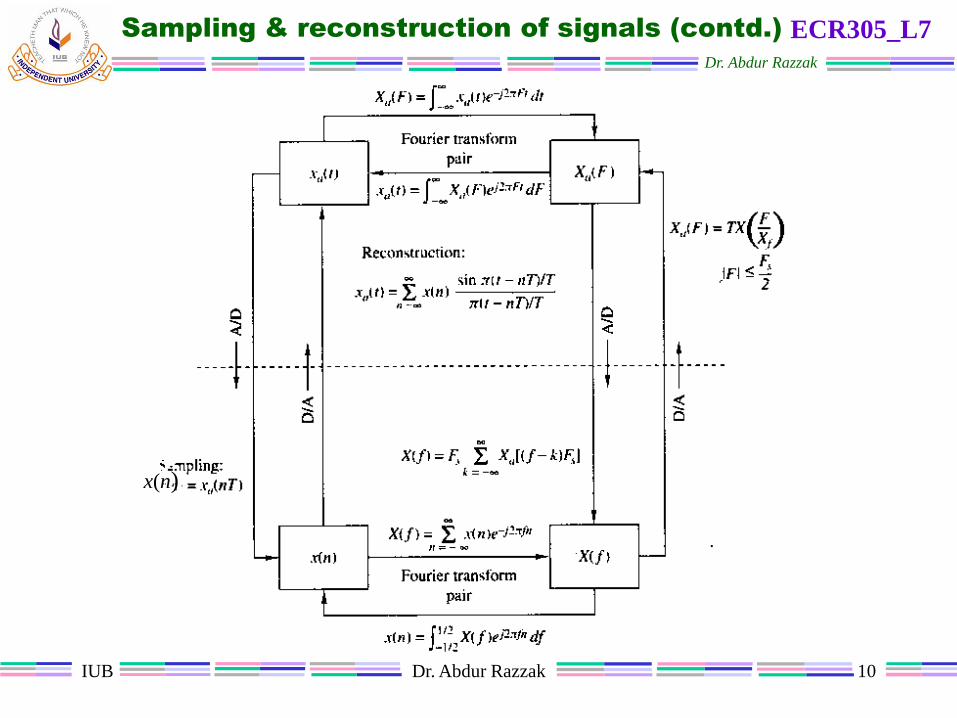
Sampling & reconstruction of signals (contd.) ECR305_L7Dr. Abdur Razzak


Band-limited signal & Sampling theorem

A signal is band-limited if there exists a finite random frequency

0 such that Xa(j) is zero for || > 0. The frequency F0 =

0/2 is called the signal bandwidth in Hz.

Sampling principle: A band-limited signal xa(t) with bandwidth

F0 can be reconstructed from its sample values x(n) = xa(nTs) if

the sampling frequency Fs = 1/Ts is greater than twice the

bandwidth F0 of xa(t).

Otherwise aliasing would result in x(n). The sampling rate of 2F0

for an analog band-limited signal is called the Nyquist rate.

02FFs



Reconstruction

If we sample band-limited xa(t) above its Nyquist rate, then we

can reconstruct xa(t) from its samples x(n). The reconstruction

follows two steps:

1. First the samples are converted into a weighted impulse train.

2. Then, the impulse train is filtered through an ideal analog

lowpass filter band-limited to the [-Fs /2, Fs /2] band.

...101...

ss

n

s TnxtxTnxnTtnx

Impulse train

conversion

Ideal lowpass

filterx(n) xa(t)



Reconstruction (contd..)

The above two-step procedure can be described mathematically

using an interpolation formula

MATLAB implementation: The sinc function can be used to

implement the above interpolation formula in MATLAB. If {x(n),

n1nn2} is given and if we want to interpolate xa(t) on a very

fine grid interval t, then the above equation

n

s

n

n

a

nTtFnxTnTtnx

TnTt

TnTtnxtx

sinc/sinc

/

/sin

21,sinc2

1

ttmtnTtmFnxtmxn

nn

ssa



Reconstruction (contd..) ECR305_L7Dr. Abdur Razzak


Sampling & reconstruction of signals (contd.) ECR305_L7Dr. Abdur Razzak

x(n)


MATLAB implementation

MATLAB

Examples

ECR 305_L7


MATLAB implementation

In a strict sense it is not possible to analyze analog signal using

MATLAB unless we use the symbolic toolbox.

However, if we sample xa(t) on a fine grid that has sufficiently

time increment to yield a smooth plot and a large enough

maximum time to show all the modes, then we can approximate

its analysis.

Let t be the grid interval such that t <<Ts. Then

can be used as an array to simulate an analog signal.

tmxmx aG



MATLAB implementation (contd..)

Similarly, the Fourier transform relation should also be

approximated as

Now if xa(t) [and hence xG(m)] is of finite duration, the above

equation is similar to discrete Fourier transform of the form

Hence the above equations can be implemented in MATLAB in a

similar fashion to analyze the sampling phenomenon.

m

tmj

G

m

tmj

Ga emxttemxjX

WxX

(5)

(6)



MATLAB example 3.18a

Let xa(t) = e-1000|t|. (a) Sample xa(t) at Fs = 5000 sample/sec to

obtain x1(n). Determine and plot X1(j).

% File name: ex3p18.m

% Analog signal

dt = 0.00005; t = -0.005:dt:0.005;

xa = exp(-1000*abs(t));

% Discrete-time signal

Fs = 5000; Ts = 1/Fs; n = -25:25;

x = exp(-1000*abs(n*Ts));

% Discrete-time Fourier transform

K = 500; k = 0:K; w = pi*k/K;

X = x*exp(-j*n'*w); X = real(X);

w = [-fliplr(w), w(2:K+1)]; % omega from -wmax to wmax

X = [fliplr(X), X(2:K+1)]; % X over -wmax to wmax interval



MATLAB example 3.18a (contd..)

% Plotting

Subplot(2,1,1);

plot(t*1000, xa);

xlabel('time in ms','fontsize',15);

ylabel('x1(n)','fontsize', 15);

title('Discrete-time signal','fontsize', 15);

hold on

stem(n*Ts*1000,x);

gtext('Ts = 0.2 ms','fontsize',12);

hold off

Subplot(2,1,2);

plot(w/pi,X);

xlabel('Frequency in pi units','fontsize', 15);

ylabel('X1(w)','fontsize', 15);

title('Discrete-time Fourier transform','fontsize', 15);



MATLAB example 3.18a (contd..) ECR305_L7Dr. Abdur Razzak


MATLAB example 3.19

Let xa(t) = e-1000|t|. Sample xa(t) at Fs = 5000 sample/sec to obtain

x1(n). Reconstruct the original signal and plot it.


% Original analog signal

t = -0.005:0.00005:0.005;

xa = exp(-1000*abs(t));

% Discrete-time signal x(n)

Fs = 5000; Ts = 1/Fs; n = -25:25; nTs = n*Ts;

xn = exp(-1000*abs(nTs));

% Analog signal reconstruction

dt = 0.00005; t = -0.005:dt:0.005;

ya = xn*sinc(Fs*(ones(length(n),1)*t-nTs'*ones(1,length(t))));

% Error calculation

Error = max(abs(xa-ya))



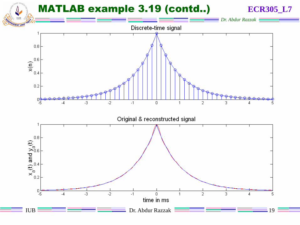
MATLAB example 3.19 (contd..)

% Plotting

subplot(2,1,1)

plot(t*1000, xa);

ylabel('x(n)','fontsize', 15);


hold on

stem(nTs*1000,xn);

hold off

subplot(2,1,2)

plot(t*1000, ya,'r');


ylabel('x_a(t) and y_a(t)','fontsize', 15);

title('Original & reconstructed signal','fontsize', 15);

hold on

plot(t*1000,xa);



MATLAB example 3.19 (contd..) ECR305_L7Dr. Abdur Razzak


MATLAB problem prob3p22

Let xa(t) = cos(20t+) sampled xa(t) at Ts = 0.005 sec intervals to

obtain x1(n). Reconstruct the original signal using the sinc

function and plot it.


% Original analog signal

t = -0.2:0.00001:0.2;

xa = cos(20*pi*t); % theta = 0 degree

% Discrete-time signal x(n)

Ts = 0.005; Fs = 1/Ts; n = -40:40; nTs = n*Ts;

xn = cos(20*pi*(nTs));

% Analog signal reconstruction

ya = xn*sinc(Fs*(ones(length(n),1)*t-nTs'*ones(1,length(t))));

% Error calculation

Error = max(abs(xa-ya))



MATLAB problem prob3p22 (contd..)

% Plottingsubplot(2,1,1)

plot(t, xa);

ylabel('x(n)','fontsize', 15);


axis([-0.2 0.2 -1.5 1.5]);

hold on

stem(nTs,xn);

grid

hold off

subplot(2,1,2)

plot(t, ya,'r');


ylabel('x_a(t) and y_a(t)','fontsize', 15);

title('Original & reconstructed signal','fontsize', 15);

hold on

plot(t,xa);

grid



MATLAB problem prob3p22 (contd..) ECR305_L7Dr. Abdur Razzak


References

1. John G. Proakis, Digital Signal Processing, Pearson, 4th

Edition, Seventh Impression, 2011. (pp. 384–440)

2. Vinay K. Ingle, and John G. Proakis, Digital Signal

Processing using MATLAB, Thomson Learning

Bookware Companion Series, 2007. (pp. 60–79)



Next class..

DFT

&

FFT


Dr. Abdur Razzak Lecture 7 Objectives

Documents

Transcript of Dr. Abdur Razzak Lecture 7 Objectives