Download report now. - Ohio Department of Natural Resources
71
Ohio Department of Natural Resources Division of Soil and Water Resources Technical Report 2011 A Functional Assessment of Stream Restoration in Ohio By Daniel E. Mecklenburg and Laura A. Fay
Transcript of Download report now. - Ohio Department of Natural Resources

Ohio Department of Natural Resources
Division of Soil and Water Resources
Technical Report
2011
A Functional Assessment of Stream
Restoration in Ohio
By Daniel E. Mecklenburg and Laura A. Fay

2
Abstract
Stream restoration has become a multi-million dollar industry while the science and techniques
are still relatively immature. A wave of early projects are now established and lend themselves to
systematic appraisals. To increase our understanding of stream restorations throughout Ohio, 51
stream restoration projects, comprising primarily physical reconfiguration, were characterized
and several elements of their ecological integrity evaluated. The stream restoration projects
assessed were constructed primarily to mitigate channel impacts from land development (94%).
The lengths of individual projects were limited (median 1117 ft). The streams affected tended to
be very small headwaters (median drainage area 224 ac).They also tended to be low energy
(median stream power, 14 lbf /(s·ft) at 2 yr peak discharge), with some very low energy more
naturally associated with wetlands (25% < 5 lbf /(s·ft) at 2 yr peak discharge). A multi perspective
evaluation of ecological integrity emphasized physical characteristics (morphology, hydraulic
process, vegetation, soil and habitat) and their deviation from natural condition. The most
striking deficiency in morphology was the lack of connectivity with a floodplain. Relative to
natural conditions, floodplains were most often both narrow and high. Performance standards
were evaluated based on their correlation with modeled floodplain connectivity. In-stream
structures were almost all riffles but indeterminately constructed for habitat or grade control.
The riffles were largely stable. However, they were often filled with fines and colonized by
wetland vegetation. Soil investigations revealed soil quality of many sites similar to reference
soils but a similar number of sites were considerably worse, dominated by subsoil with poor
consistence and low organic matter, permeability or root density. Predicting the quality of soil
characteristics (R2=0.69, P<<0.001) was best achieved by weighing the amount of in-situ and
depositional A horizon against the amount of in-situ and constructed C horizon. The headwater
habitat evaluation index (HHEI) scores showed virtually no correlation with other characteristics
of ecological integrity. The only significant correlation was a positive correlation with stream
power. The success of the observed stream restoration projects, as measured by several aspects
of physical condition, varied widely despite meeting required permit performance criteria. The
results of this study demonstrate a need for physical standards for restoration projects that
physically reconfigure streams.

3
Acknowledgements
The Ohio Department of Natural Resources, Division of Soil and Water Resources wishes to
thank the Ohio Water Development Authority (OWDA) for funding for this project.
The authors wish to thank the many people who provided recommendations for sites to be
studied and those who provided technical documents about the projects from the Ohio
Environmental Protection Agency and the Army Corps of Engineers districts. At Ohio EPA, special
thanks go to Mike Smith for input and feedback throughout the project. Also at Ohio EPA,
thanks to Randy Bournique, Dan Osterfeld, Paul Anderson, Dennis Mishne, Matt Fancher and
Jeffrey Boyles. At the Army Corps of Engineers Huntington District, thanks to Jim Spence and
Denise Marmer for providing data reports.
Thanks also to Drs. Andy Ward, Jon Witter and Jay Dorsey for input on data analysis.
This project could not have been completed without the soils’ expertise and efforts of Steve
Prebonick, Brian Cooley, Neil Martin, Matt Deaton and Tim Gerber.

4
Table of Contents Abstract ........................................................................................................................................... 2
Acknowledgements ......................................................................................................................... 3
Introduction ..................................................................................................................................... 8
Background .................................................................................................................................... 10
Stream Restoration Monitoring and Assessment ..................................................................... 10
Ecological Integrity .................................................................................................................... 11
Monitoring and Assessment in Ohio ......................................................................................... 11
Physical Integrity ....................................................................................................................... 12
Methods ........................................................................................................................................ 15
Selection of Study Sites ............................................................................................................. 15
Morphology ............................................................................................................................... 16
Soil Investigation ....................................................................................................................... 18
Habitat Assessments ................................................................................................................. 20
Results and Discussion .................................................................................................................. 21
Inherent Site Characteristics ..................................................................................................... 21
Morphology ............................................................................................................................... 24
Soil Investigations ...................................................................................................................... 38
Stream Channel Habitat Assessments ....................................................................................... 44
Summary and Conclusion .............................................................................................................. 49
References ..................................................................................................................................... 57
Appendix ........................................................................................................................................ 64

5
Figures
Figure 1 Ecological integrity is the integration of a hierarchy of many simpler functions down to
individual ecological services.
Figure 2 Water movement through streams emphasizing pathways between channel and
riparian area.
Figure 3 Distribution of drained lands in the United States.
Figure 4 Assessed project site locations.
Figure 5 Example of Soil Data Sheet.
Figure 6 Reconfigured stream channel length.
Figure 7 Reconfigured channel length measured relative to the 401 permit required channel
length.
Figure 8 Watershed size contributing to project streams.
Figure 9 Local channel slope.
Figure 10 Stream energy presented as stream power of the 2-yr peak discharge.
Figure 11 Channel size shown as the recurrence interval (RI) of bankfull flow rate.
Figure 12 Bankfull discharge as a percentage of the 2 yr RI peak discharge.
Figure 13 The 50 yr RI flood stage estimated for 54 stream reaches is shown as multiples of two
depth values, observed and estimated from a regional curve.
Figure 14 Entrenchment ratio based on regional curve derived channel dimensions and
observed dimensions.
Figure 15 Adjusted Flood Prone Area shown as areas saturated or inundated at three stages
with higher areas weighted less.
Figure 16 Floodplain extent for stream reaches with slopes less than 2%, in relation to natural
floodplain target width.
Figure 17 Example of floodplain inundation stages and the associated number of occurrences
for stages of recurrence intervals: 0.8, 1.6, 3.2, 6.4, 12.5, 25, 50, and 100 yr.
Figure 18 Floodplain connectivity in terms of the area of floodplain-flood exposure relative to a
benchmark condition. Floodplain exposure is the cumulative area inundated by 100 yrs of
statistically predicted storms.
Figure 19 Bankfull stream power of assessed channels is shown based on two methods, the
observed bankfull channel and a standard bankfull recurrence interval flow (0.8 yrs).
Figure 20 Unit stream power values shown, based on 2-yr peak flow rate and regional channel
dimensions and based on measured bankfull channel.

6
Figure 21 Unit stream power of the assessed streams relative to three reference data sets.
Figure 22 Sinuosity of 52 channel reaches, the first 19 of which have no meandering.
Figure 23 Sinuosity can be limited by the width of the floodprone area.
Figure 24 Ratio of the bed material observed to the expected natural mobile riffle material
indicates that the placed material at these sites was predominantly several times larger than
naturally occurring riffle material.
Figure 25 Dark stain on rock from embedded riffle indicating chemical reduction.
Figure 26 Riffle colonized by hydrophytic vegetation at the Slane residential site.
Figure 27 Constructed meandering channel colonized by vegetation at Millersburg Walmart site.
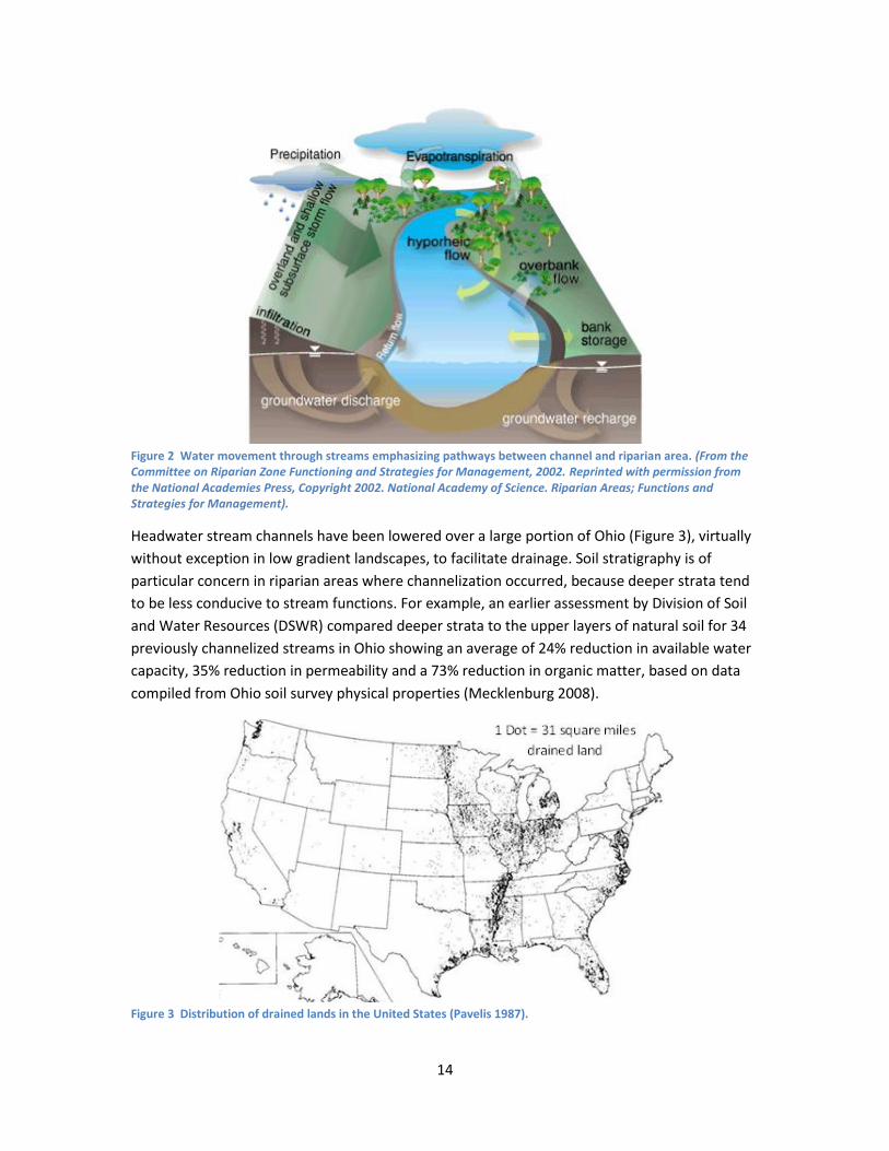
Figure 28 General soil health of sites ordered. The top site had the best average of five
individual soil characteristics rank.
Figure 29 Individual soil characteristics from the 22 stream restoration soil investigations ranked
best overall and the 22 ranked worst compared to 18 soil investigations of natural references.
Figure 30 Characteristics of the A, B and C horizons by soil origin, reference natural condition,
deposition post construction, in-situ, used in place, placed during construction.
Figure 31 The prevalence of four of the horizon origins had a correlation with the soil
investigation ranking.
Figure 32 Soil profiles with the combination of the most depositional or in-situ A horizon and
the least constructed or in-situ C horizon had the closest correlation with general soil health.
Figure 33 Habitat Types of 54 stream reaches.
Figure 34 HHEI scores are shown by column height for all fifty-four stream reaches assessed.
Figure 35-A, B, C HHEI scores verses in-channel vegetative density, floodplain connectivity, and
riparian soil health.
Figure 36-A HHEI scores trend lower for newer more recent projects.
Figure 36-B HHEI corresponds with inclusion of projects on low energy streams.
Figure 37 HHEI score has a high correlation with stream power, higher than any other
independent variable observed.

7
Tables
Table 1 Vegetation density of four sites examined to illustrate the contrast of vegetation density
of some stream channels and floodplains. Sites were selected for dense channel vegetation.
Appendix Table A Project stream information
Appendix Table B Discharge rate and stream power
Appendix Table C Floodplain widths
Appendix Table D Floodplain connectivity
Appendix Table E Channel and floodplain vegetation and roughness
Appendix Table F Riffle surface material
Appendix Table G Soil characteristics weighted score and functional health ranked best to worst
Appendix Table H Habitat index scores and channel vegetation characterization.

8
Introduction
The physical alteration of stream channels has been taking place in Ohio since the mid-1800s.
Tens of thousands of miles of streams have been channelized (Pavelis 1987). This monumental
effort was undertaken primarily to improve the use of the land through improved drainage or
reduced flooding (Keller 1976, Brookes 1988, ODNR 2008 and ODNR 2009). Only recently has
ecological integrity become a common goal for channel work. While streams continue to be
modified for drainage and flood control, there is now the added expectation for many of these
projects to minimize ecological impacts. In addition, a growing number of channel modification
projects now are undertaken for the sole purpose of improving ecological condition (Shields et
al 2003 and Bernhardt et al 2005).
No one term precisely encompasses the projects assessed in this report, so we will imperfectly
refer to them all as restoration. What constitutes stream restoration has been debated at
length (NRC 1992 and Shields et al 2003). Noting that restoring pre-settlement conditions is
rarely obtainable, restoration has been proposed to mean restoring the biota and ecological
processes and services (Shields et al 2003, 33 CFR 332.2). This partial restoration has
alternatively been described with terms such as renovation and rehabilitation. Either way the
idea implied is to improve the existing condition, which is not necessarily the case. For example,
where land development impacts a quality stream, the goal is to minimize ecological impacts.
Most projects have been constructed for reasons other than ecological improvement. By
restoration, we mean only that, within site constraints, one of the project goals was to maximize
ecological condition.
Typically, stream restoration projects have occurred for mitigation, defined by Shields et al
(2003), as “an activity to compensate for or alleviate environmental damage. Mitigation may
occur at the damaged site or elsewhere. It may also involve site restoration to an acceptable
condition, but not necessarily to a natural condition”. Not included in this report are projects
that provide stream preservation or stream bank stabilization for infrastructure protection
which are sometimes confusingly lumped together with restoration.
Ecological restoration may at times consist of manipulation of the biota including planting trees,
reintroduction of species or control of invasive species. However, for the purposes of this study,
stream restoration projects are limited to those that involve reconfiguration with a substantial
change in channel form.
In spite of having no concise definition, the types of projects reviewed in this report
demonstrate an initial attempt at implementing a new norm for the physical alteration of
stream channels. Enough projects have been constructed and are becoming established to allow
for meaningful evaluation. Learning from these projects was the goal of this assessment,
specifically better understanding which techniques are most appropriate for assessment,
evaluation and measuring success, and identifying elements of standards and guidelines that will

9
lead more efficiently to successful projects. For stream reconfiguration projects, undertaken at
least in part to benefit ecological integrity, this report will:
• describe the characteristics and types of streams being restored,
• evaluate restoration success based on an array of ecological functions,
• explore methods understood to be integral with the ecological function,
specifically elements of physical condition influenced by reconfiguration
projects that may serve as practical indicators of less tangible ecological
functions.

10
Background
Stream Restoration Monitoring and Assessment Although the terms stream mitigation, restoration, renovation, reclamation and rehabilitation
have been used throughout the scientific literature for several decades; the science is still
relatively immature (Tompkins and Kondolf 2007). Early on, Kondolf (1996) encouraged
systematic studies to evaluate the success of stream mitigation projects attempting to restore
ecological function. The lack of pre-project and post-project multi-disciplinary data was seen as
a weakness in the scientific community’s ability to collectively learn about each project’s
effectiveness. Kondolf recommended monitoring a broad array of stream characteristics to
accumulate knowledge on successes and failures.
A database of 1,345 stream restorations constructed between 1970 and 2004 in the upper
Midwest (Michigan, Ohio and Wisconsin), was compiled by Alexander and Allan (2006) as part of
the National River Restoration Science Synthesis project to evaluate the effectiveness of
commonly used stream restoration practices. Alexander and Allan emphasized the need for
more detailed and standardized evaluation. The monitoring results that did exist were generally
discouraging. Fewer than half of the 1,345 regionally completed projects evaluated by Alexander
and Allan (2007) were described as ecologically successful. According to Alexander (2005) in her
study of Michigan, Wisconsin and Ohio streams, the majority of the restoration projects were
not sustainable and chemical parameters showed no change after restoration indicating that the
stream’s assimilative capacity had not increased. Rather than seeing improved watershed scale
results, Alexander and Allan (2006) observed a trend toward increasing project costs and
decreasing project lengths over time, indicating more money was being spent on smaller and
more expensive projects. They also noted an increasing tendency to refer to channel
stabilization projects as restorations. According to the National River Restoration Science
Synthesis project, many projects were implemented to address the symptoms of an
environmental concern without first understanding the larger scale processes underlying the
observed environmental degradation (Tompkins and Kondolf 2007).
Two notable methods have been proposed specifically for ecological assessment of stream
restoration. The first is the post project appraisal (PPA) protocol described by Downs and
Kondolf (2002) which was an exhaustive list of physical assessments with streamflow data;
conveyance data; channel roughness; channel cross sections; longitudinal profile; channel bed
material; aquatic habitat mapping; mapping emergent, riparian and floodplain vegetation;
floodplain deposition samples; and comparisons of historical aerial photos. Another assessment
method proposed was more a list of guiding principles. Palmer et al (2005) suggested
restoration: 1) be based on an image of a dynamic healthy river; 2) measurably improve
ecological condition; 3) be self-sustaining and resilient to external perturbations; 4) cause no
lasting harm; and 5) have pre and post-assessments completed and publicly available. These two
very different restoration assessment methods are ecologically comprehensive. However,
neither provides much specific guidance or definitive criteria for stream restoration regulation

11
or design. Well-founded stream restoration tools and assessment methods are not yet broadly
established.
A third method is specifically a tool for the review of stream restoration proposals called
RiverRAT for River Restoration Assessment Tool. It was developed by NOAA Fisheries and US
Fish and Wildlife with an emphasis on west coast salmonid stream restorations. It starts with 16
questions regarding problem identification, the technical basis of the design and adequacy of
assessment measurements. It goes on through links to a companion document, “Science Base
and Tools for Evaluating Stream Engineering, Management and Restoration Proposals” to
provide an in-depth resource suitable for large stream restoration challenges.
Ecological Integrity Ohio’s stream mitigation/restoration programs have a sound conceptual foundation based on
ecological integrity, defined by Karr and Dudley (1981) as the ability of a system to maintain and
repair itself. Smith et al (1995) explained ecological integrity as the integration of nested
ecological functions composed of a hierarchy of the all things a system does, starting with the
individual processes such as nitrogen removal, flood control or support for a specific biotic
community as simple functions nested in broader processes all the way to the most complex,
ecological integrity, which is the maintenance of all the integrated functions (Figure 1). This
conceptual framework connects broad stream functions to measurable stream characteristics.
The denitrification process, for example, necessarily entails denitrifying bacteria and organic
matter in anoxic conditions. Peak flow attenuation by the process of flood routing is determined
by measurable floodplain form and quantifiable channel and floodplain roughness. Vegetation
communities require light and soil with quantifiable characteristics.
Some components of ecological integrity are influenced by stream projects more than others. In
this assessment, an attempt was made to evaluate component variables most sensitive to the
physical modifications of stream reconfiguration.
Figure 1 Ecological integrity is the integration of a hierarchy of many simpler functions down to individual ecological services (adapted from Fennessy, 2007 and Smith 1995). The simpler the function, the easier it is to describe by quantifiable structure and process variables.
Monitoring and Assessment in Ohio An advantage when conducting monitoring and assessment studies in Ohio is that Ohio EPA’s
Division of Surface Water has been a national leader in using biological indicators to assess
overall stream ecological integrity. Ohio EPA has developed a widely used Index of Biotic
Ecological Integrity
Biogeochemical Cycling Hydrology Biological Diversity
Nitrogen
Cycling
Vegetation
Diversity
Hydrologic
Connectivity
Nitrogen
Removal
Vegetation
Community
Flood
Control
12
Integrity (IBI) tool for fish assessment, an Invertebrate Community Index (ICI) tool for
macroinvertebrates, and the Qualitative Habitat Evaluation Index (QHEI) and Headwater Habitat
Evaluation Index (HHEI) tools for habitat quality assessment.
Ohio EPA recently initiated a study of the effects of stream restoration on fish and
macroinvertebrate communities. Two years of pre-restoration data have now been collected
(Ohio EPA 2009b and 2010a). Post construction studies by Ohio EPA will document the
effectiveness of the biological recovery. These Ohio EPA biotic studies are specifically on Clean
Water Act Section 319 funded stream restoration projects and do not include Clean Water Act
Sections 401/404 permitted stream mitigation projects which tend to be relocated channels on
developed sites rather than streams selected for restoration.
The 401/404 projects are monitored by the permittee, generally for stability, habitat and any
special permit conditions. The monitoring period is a minimum of five years post construction
with annual reports submitted to Ohio EPA and the US Army Corps of Engineers, both of which
make site visits in the third and fifth year.
Compared to Ohio’s established stream monitoring programs that assess the overall condition
of Ohio’s streams, monitoring more applicable to stream reconfiguration projects is still
developing. Generally, assessment of physical integrity is now limited to aspects of habitat.
By comparison, considerable monitoring work that includes key physical attributes has been
completed for Ohio wetlands. Ohio EPA generated four studies on the effectiveness of wetland
restoration (Fennessy and Roehrs 1997, Porej 2003, Kettlewell 2005 and Micacchion et al 2010)
and one report on the ecological effectiveness of wetland mitigation banks (Mack and
Micacchion 2006). Ohio EPA developed the Ohio Rapid Assessment Method (ORAM) screening
tool to determine the integrity of wetlands and the likelihood a comparable wetland could be
created elsewhere. Ohio EPA also requires that the functions of mitigated wetlands be assessed
and compared to natural wetlands using one of several OEPA vegetation, macroinvertebrate or
amphibian wetland assessment tools (Micacchion 2004, Mack 2007 and Ohio EPA 2004a). Ohio
EPA has used the results and conclusions of these wetland studies to better clarify the physical,
chemical and biological requirements for future mitigated wetlands to be created under Section
401 requirements.
Physical Integrity Water quality is a compilation of physical, chemical and biological integrity as defined by the
Clean Water Act, the cornerstone protection for surface water quality. Since 1972 and the
promulgation of the Federal Water Pollution Control Amendments, including The Clean Water
Act, projects that physically changed streams by moving the centerline or placing fill required a
permit and mitigation activities for those impacts.
Even though there is a lack of broadly established stream restoration assessment tools, there
appears to be agreement that morphology, or the study of form, is a logical part of stream
13
assessment. (This seems particularly apt for restoration involving stream reconfiguration.)
Morphological assessments are based on direct measurements of the channel cross sectional
dimension, longitudinal profile and meander pattern (Richards 1982). Stream form and process
are inextricably coupled and thus an extension of direct measurement of stream form provides
estimates of processes that take place at various flow rates. Vegetative roughness, velocity,
shear stress and stream power are but a few of the process values routinely estimated as part of
stream morphology assessment (Rosgen 1996).
Morphology assessment includes the entire area of the stream, not just the narrow strip
typically wetted by daily flow but instead the entire width covered by high flows. Assessment of
the floodplain is valuable because stream processes are largely episodic, during periods of high
flow (Kondolf 2006). The flood pulse concept postulated by Junk, Bayley and Sparks (1989)
described stream functions responsible for the productivity of river-floodplain systems as “batch
processes” occurring at high flow. Palmer (1976) proposed the concept of a streamway to be
inclusive of the portion of the valley that the dynamic meandering stream system occupies over
time. The compound form that most natural channels exhibit with relatively broad floodplain
and narrow channel allows streams to be self-maintaining through low flows and floods with a
range of energy that crosses orders of magnitude (Leopold 1994). Thus, the forms that streams
take at all flow rates are key to the evaluation of stream morphology.
A standard technique used in stream morphology is scaling proportional to the channel itself.
The bankfull channel is consistently associated with those intermediate discharge rates that are
both powerful enough and occur frequently enough to be most influential in the channel
forming processes (Dunne and Leopold 1978). The bankfull channel dimensions commonly serve
to normalize measured values and allow comparison of the characteristics of different size
streams. For instance, floodplains can be described in terms of the number of times wider than
the bankfull channel width. A floodplain 20 times wider than its bankfull channel is extensive
whether it is a little headwater stream or a major river. Similarly, flood stages are expressed in
multiples of the bankfull channel depth. For example, the width of flow at the stage two times
the maximum bankfull channel depth defines the often-used term floodprone width (Rosgen
1994).
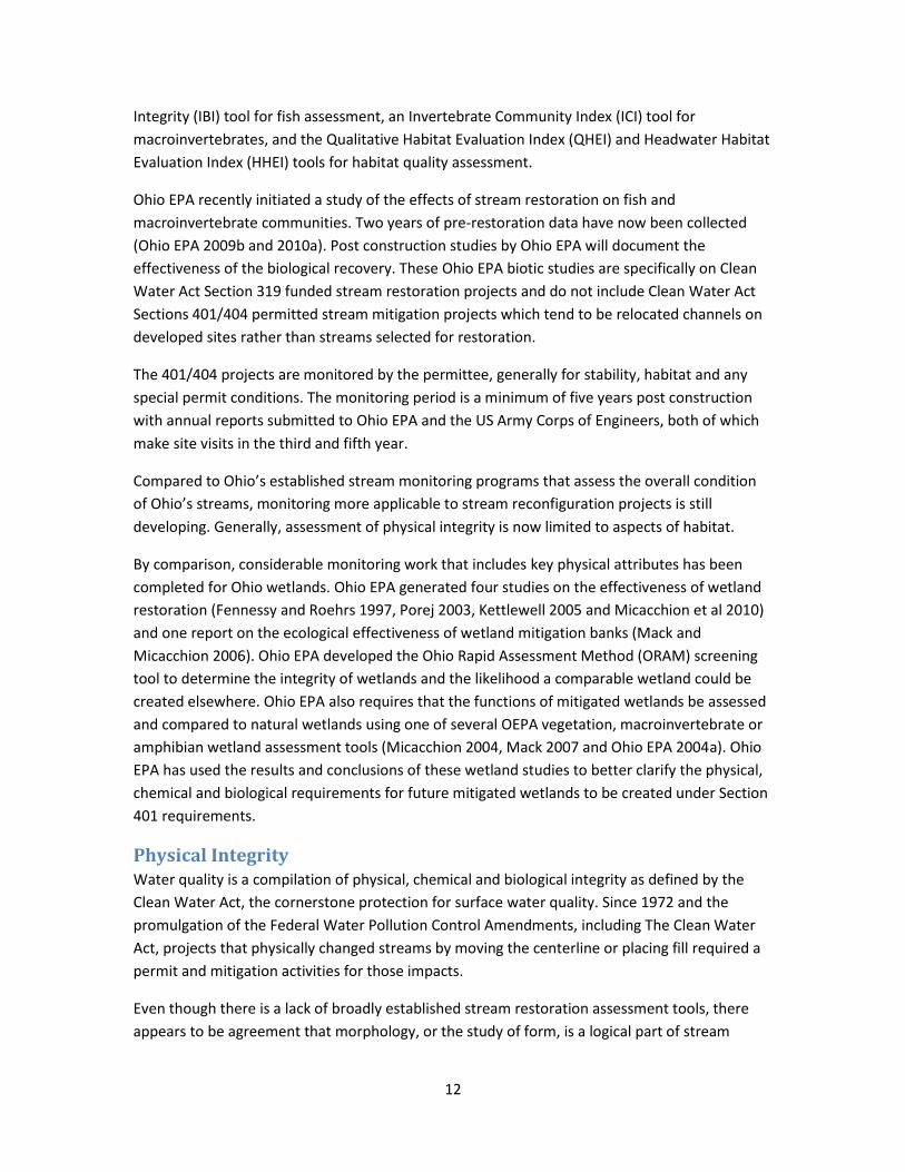
In addition to a stream’s form and processes, another physical aspect is the material of which it
is composed, its subsurface lithology. Streams do not simply flow over an impermeable two-
dimensional surface, but flow through banks, beds and floodplains laterally and vertically (Figure
2). Ground water and shallow hyporheic water flow through channel bed material and riparian
soils. Van der Putten (2004) described the ecological services provided by natural floodplain soils
including retention of nitrogen in biomass, physical stabilization, interception of runoff,
moisture retention, evapo-transpiration and carbon sequestration. For these, he described the
necessity of soil supporting soil organisms (bacteria, fungus, nematodes, protozoa, earthworms
and isopods). The material composition of a streamway has an intricate role in its ecological
functions and is certainly manipulated by restoration work.
14
Figure 2 Water movement through streams emphasizing pathways between channel and riparian area. (From the Committee on Riparian Zone Functioning and Strategies for Management, 2002. Reprinted with permission from the National Academies Press, Copyright 2002. National Academy of Science. Riparian Areas; Functions and Strategies for Management).
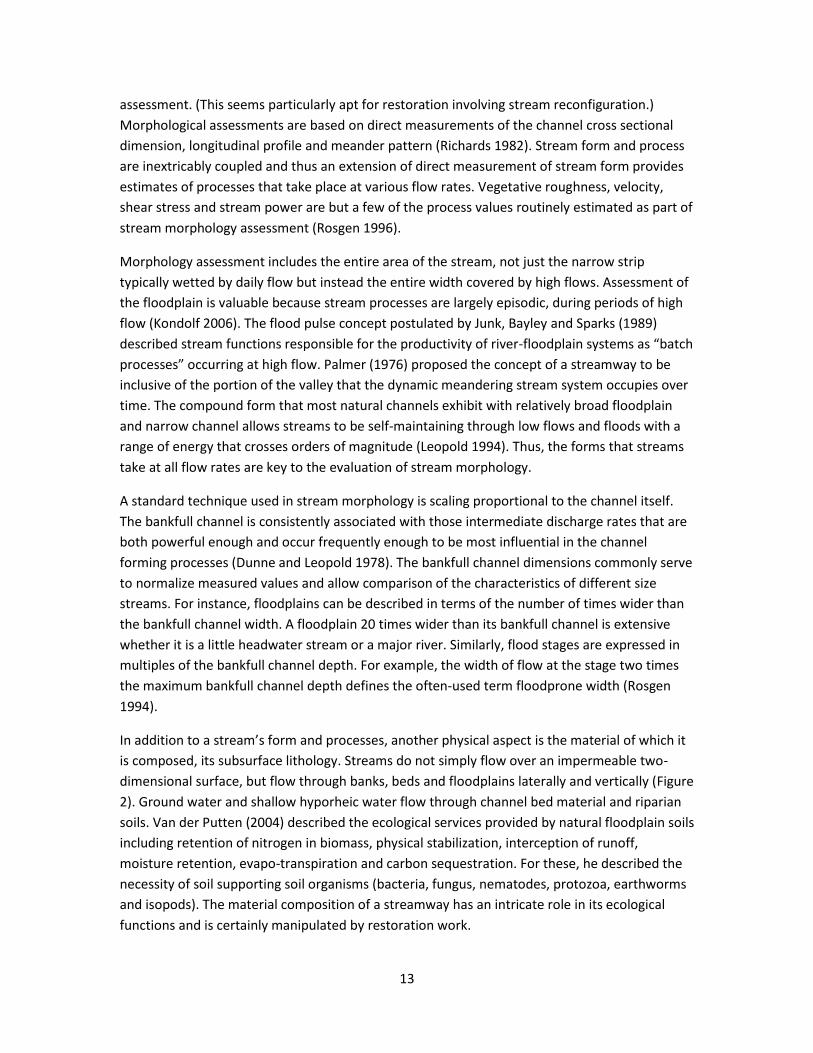
Headwater stream channels have been lowered over a large portion of Ohio (Figure 3), virtually
without exception in low gradient landscapes, to facilitate drainage. Soil stratigraphy is of
particular concern in riparian areas where channelization occurred, because deeper strata tend
to be less conducive to stream functions. For example, an earlier assessment by Division of Soil
and Water Resources (DSWR) compared deeper strata to the upper layers of natural soil for 34
previously channelized streams in Ohio showing an average of 24% reduction in available water
capacity, 35% reduction in permeability and a 73% reduction in organic matter, based on data
compiled from Ohio soil survey physical properties (Mecklenburg 2008).
Figure 3 Distribution of drained lands in the United States (Pavelis 1987).

15
Methods The physical condition of restored streams was investigated using multiple disciplines:
morphology, vegetation, soils, and habitat. Characteristics were selected for their key functional
roles in the nested scheme of ecological integrity.
Selection of Study Sites For this study, 51 projects involving substantial channel modification were selected for
monitoring from the total 518 permits issued in Ohio from 1996 to 2007. Permitted stream
projects were those regulated by Ohio EPA Division of Surface Water’s 401 Section, the United
States Army Corps of Engineers’ Nationwide permit 27 and 38, and Superfund cleanups (Figure
4).
Figure 4 Assessed project site locations. http://maps.google.com/maps/ms?ie=UTF8&hl=en&msa=0&msid=107960685558029914341.000452b1247b2a72059da&ll=40.375844,-82.650146&spn=4.017137,6.696167&t=p&z=8
The Ohio EPA’s 401 Section provided DSWR a list of all projects that authorized stream impacts
and required stream mitigation. Four hundred thirty six Section 401 projects were issued for
stream impacts between 1996 and February 7, 2007. DSWR also obtained lists of 10 stream
projects that were issued permits by the Army Corps of Engineers under Nationwide 38

16
(Cleanup of Hazardous and Toxic Waste) and 71 stream projects issued permits under
Nationwide 27 (Aquatic Habitat Restoration, Establishment and Enhancement Activities).
Superfund cleanups, by law, do not require either Clean Water Act 401 or 404 nationwide
permits but are required to comply with substantive applicable, appropriate and relevant
requirements (ARARs) from these types of permits. DSWR obtained information on one
Superfund site (Fieldsbrook) that was comparable to the types of remediation efforts conducted
in Nationwide 38 projects.
The combined list of 518 permitted projects included many that were predominantly bank
armoring, riparian plantings, utility crossings and stream preservation, with little or no channel
modification. The project descriptions were reviewed to identify mitigation that included
substantial channel work. Recurring keywords such as restoration, relocation or remediation
helped in the selection of projects with channel work. Permit administrators were also queried
to help distinguish between projects with or without substantial channel work. Projects
assessed were limited to those constructed from 1997 to 2006, limiting the variation in age and
ensuring at least three years had passed post construction prior to the 2009 monitoring season.
This review and evaluation resulted in a list of 51 permitted projects, one of which had two
modified streams, resulting in 52 streams monitored and another project had three distinct
designs in series, making the number of restored stream reaches 54.
Morphology Channel dimension, pattern and profile were surveyed for each project. While conditions
sometimes differed considerably within some sites, no attempt was made to describe the range
of conditions. Rather, a reach was selected that appeared to be most representative of the
project. If the stream generally appeared consistent, a section near the middle of the project
was assessed.
The stream surveys largely followed the field technique described by Harrelson et al. (1994)
using a laser level and survey tapes for the collection of stream channel measurements.
Additionally a handheld GPS and Google Earth imagery supplemented channel pattern
measurements. Measurements included bed and water surface elevations, changes in
vegetation, top of bank, and indicators of channel formation (i.e., depositional surfaces such as
benches, bars and breaks in the slope of the bank). Within each reach, two to four cross sections
typically were surveyed as necessary to characterize the channel and the valley. For stream sites
with uniform cross sections (e.g., Southgate Industrial Park) only one cross section was
surveyed.
Surface bed material was assessed at riffles. An attempt was made to distinguish between
mobile riffle surface material and material placed during construction. Pebble counts were
performed for gravel and coarser material according to Ward and Trimble (2004) based on the
technique by Wolman (1954). Silt and clay bed material was recorded based on visual and tactile
observation. Embeddedness was noted as highly or moderately embedded as evidenced by silt
and clay filling gravel or cobble interstices. Black staining on the buried portions of large

17
particles and the absence of macroinvertebrates on those surfaces were used to indicate anoxic
conditions.
Survey data were reduced and analyzed using a modified version of The Reference Reach
Spreadsheet Version 4.3L of STREAM (Spreadsheet Tools for River Evaluation, Assessment and
Monitoring) (Mecklenburg and Ward 2005)
Hydrology: Instantaneous peak discharges were estimated for the 2 to 100 yr recurrence
interval (RI) events using USGS’s Ohio urban and rural equations (Koltun and Whitehead 2001,
and Koltun 2003). Peak discharges were then interpolated and extrapolated for an expanded
doubling series, 0.2, 0.4, 0.8, …50, 100 yr RI, as described by Mecklenburg and Ward (2002) and
(Powell et al 2006)
Hydraulics: The Reference Reach Spreadsheet was modified to analyze not just bankfull flow,
but also the flow at a stage equal to the regionally predicted maximum bankfull depth and each
of the 10 peak discharge rates of the recurrence interval series from 0.2 to 100 yrs. At each
stage, only the cross sections appropriate for describing that stage were selected for analysis.
For example, a riffle crossing over between two outside bends might be the best location for
describing in-channel flows, but to describe flood flows a cross section perpendicular to the
valley may be more suitable.
Manning’s roughness coefficients were selected for three stages; low flow (0.2 yr RI), high flow
(100 yr RI) and at bankfull (the flow stage associated with major breaks in the cross sectional
geometry). Estimates of roughness were made iteratively to allow the effects of relative
roughness and vegetation submergence to be accounted for in the determination. A
spreadsheet macro was written to find the flow stage with the flow rate that matched the
hydrologically predicted peak discharge for each recurrence interval. Roughness coefficients for
these three stages were selected using Chow (1959) and Barnes (1967). Channel and floodplain
roughness coefficients for peak discharges of recurrence intervals between the three stages
were assigned values by interpolation.
Vegetation Assessments: Vegetation varied considerably from site to site and within individual
sites. Several assessment methods recorded characteristics of vegetation. The density of
vegetation was recorded on a range from dense and vigorous to sparse and separately by zone:
channel bed, riffles, bankfull channel, near bank and floodplain. Root density, quantified during
the soils investigation, is another measure of riparian vegetation. Manning’s roughness
coefficients further reflected the vegetation. Lastly, the basal area method was explored. This
assessment technique, as defined by Bonham (1989), involves cutting and bundling the
vegetation within a 1-meter square PVC quadrat, then measuring the circumference of the
bundle for the total stem density using the linear diameter measure technique of Pearse (1935)
and described by Bonham (1989). Vegetation assessments were done at randomly selected
locations in both the channel and the floodplain for four sites.

18
Soil Investigation Soil scientists from the Ohio DNR, Division of Soil and Water Resources applied the techniques
and skills established for soil mapping and land capability analysis to assess riparian soil quality.
This approach to the soil investigations was selected for the comprehensive view of soil health it
provides.
Sampling locations within the projects site were selected to be representative of the active
floodplain. The investigation went to a depth equivalent to the elevation of the adjacent
streambed such that the soils described are those that interact most with the stream during
periods of low flow as well as floods. At several sites, more than one investigation was
performed to describe substantially different conditions. A corresponding reference condition
investigation was performed for approximately half of the sites. This entailed the initial
identification of potentially undisturbed riparian soil near the site was initially identified using
remote imagery with the final location selected by the soil scientist in the field. No soil
investigations were performed for four of the projects that were highly entrenched with no
discernable floodplain. A total of 77 soil investigations were performed during the study.
Soil investigations involved excavation of pits by hand spade, followed by deeper excavation
with a bucket auger. Soil characteristics of color, redoximorphic features, texture, organic
matter, structure, consistence, and roots were recorded based on the methods of USDA NRCS
(2002). The origin of each horizon was recorded as constructed (re-soiled) material, soil
deposited or accumulated post construction, or natural material left in place although material
may have been removed above it. Soil profile horizon thickness was recorded using
nomenclature as established by the Soil Survey Staff (1998, 1999). A sample of the form can be
seen in Figure 5. A more detailed description of soil investigation techniques is in Appendix A.
Figure 5 Example of Soil Data Sheet
County: Medina Land Use: use is a natural area Date: September 18,2008
Location: Vegetation: honey locust, weeds, grass Evaluator: Steve Prebonick
Regional Curve: Mid Ohio Landform: floodplain
Drainage Area: 0.42 Position on Landform: flat Method
Watershed: Percent Slope: 0.5 Pit: X
Project Name: Brunswick Town Center Test Hole #: B ( south side of the drain) Auger: X
Site Name: Site B Latitude / Longitude: N 41 14 07.6 W 81 48 27.1 Probe:
Redoximorphic Features Texture Clay Frags OM Structure Consis- Tyler Effer-
Horizon Top Bottom Matrix Consentrations Deletions Class (%) (%) (%) Grade Size Shape tance Rate Roots vesence Origin
A 0 0.2 10YR 4/2 SiL 7 0 3 1 f gr Fr 0.6 M f&vf D
2C 0.2 5 10YR 4/2 CL 31 7 2 0 m Fi 0 C f&vf es C
3C1 5 20 10YR 5/4 CL 32 10 0.3 0 m Fi 0 es I
3C2 20 36 10YR 5/4 7.5YR 5/6 GR-L 23 25 0.3 0 m Fr 0.5 e I
Width of water in channel: 7 feet Additional notes:
Distance from center of channel: 30 feet
Relative elevation above water surface: 30 inches
Depth (in)
Soil Profile Saturation - Munsell Color Soil Permeability
flooding area 50 to 60 feet wide ; A horizon is recently deposited flood plain
sediments; 2C horizon is a mixture of topsoil and subsoil fill; 3C1 horizon is original
parent material; 3C2 is original parent material

19
Soil Profile - Soils are described in layers called horizons. Depth and characteristics of each
horizon were recorded. Generally, there are three basic horizons, A, B, and C. The A horizon is
normally the top layer of soil called topsoil. This layer has the largest accumulation of organic
matter and is the most biologically active. The next deeper horizon is the subsoil or B horizon
which is often divided into subhorizons with letters indicating conditions in which they formed.
The C horizon is not actually soil but parent material, and has far less structure and organic
matter, and more restricted root growth compared to the upper horizons. C horizons are usually
far less permeable although occasionally layers of sand and gravel may actually make them
more permeable.
Soil Texture is the percent sand, silt, and clay correlated to the USDA textural triangle for the
textural class. It affects water holding capacity, water movement, and root growth. Soil texture
was estimated in the field by hand, using the ribbon method as described by Thien (1979).
Soil Organic Matter accumulates from roots and when organic matter deposition exceeds
decomposition, and strongly influences microbial and chemical activity, water movement and
root growth. The percent of organic matter was estimated with visual-manual field methods
using the Color Chart for Estimating Organic Matter in Mineral Soils in Illinois (University of
Illinois Extension 1995).
Soil Structure was characterized by three variables - grade, size and type - according to the
National Soil Survey Center, NRCS, USDA (Schoenberger 2002). Soil structure characterizes the
tendency of a soil mass to break along distinct planes. Well-developed soil structure increases
soil permeability and facilitates root growth. Soil structure can be lost in cut and fill operations
and by compaction caused by construction activities. Once structure is destroyed, it typically
takes a very long time to redevelop, especially in the lower horizons. When stream restoration
projects are relocated into parent material (C horizon), it could take up to 1000 yrs for this
material to develop into soil (Jenny 1994).
Soil Consistence describes soil resistance to deformation and strongly affects water movement,
water holding capacity, and root growth. Visual-manual methods for field determinations take
into account resistance to rupture, resistance to penetration, plasticity, and toughness (Soil
Survey Division Staff 1951). The observations recorded are loose, very friable, friable, firm, and
very firm. Topsoil with good tilth is typically very friable or friable. DSWR Soil Scientists set a
numeric scale of consistence quality for use in calculating a single depth weighted average score
for each profile. The scale values were 3 for both loose and very friable, 2.5 for friable, 0.5 for
firm and 0 for very firm.
Soil Permeability is the rate of water movement through the soil profile. It is a complex product
of various soil morphological characteristics and processes. The Tyler loading rate (Tyler 2001)
was chosen as a practical indicator of soil permeability but also because of its established
correlation with microbial activity (Tugel and Lewandowski 1999) and nutrient uptake rate
(Doyle 2003). The Tyler loading rate was developed to assign hydraulic wastewater loading rates

20
to soil based on combinations of soil texture, structure type, and structure grade. These soil
characteristics are observed and recorded along with a rating from the Tyler Chart (Tyler 2001).
While the loading rate values have units of gallons/day/ft2, these units are not applicable to
floodplain processes. Instead, the Tyler loading rate values are used as a unitless scale starting
at zero indicating a restrictive soil horizon with water movement in such horizons very slow with
restricted root growth. Horizons that are more permeable have higher values on the scale. For
example, an undisturbed loam with excellent structure is assigned a value of 0.8. The high end
of the scale is 1.6 for the least restrictive soil horizon, such as coarse sand with the most
potential infiltration.
Root Density was estimated in the field according to the protocol defined by the National Soil
Survey Center (Schoenberger 2002). For each soil horizon, roots were indicated as many,
common, few, and very few. To calculate a single depth weighted average score for root density,
a numeric scale corresponding to the root density designations was defined. DSWR soil scientists
reviewed the National Soil Survey Center protocol, debated and reached consensus on a root
density scale of 4, 3.5, 2.5 and 0 for the designations many to very few.
Soil Origin is the soil morphogenesis as related to the restoration project. Each soil horizon was
categorized as an undisturbed natural in-situ layer (I), as placed during project construction (C),
or as deposited post project construction (D). The designation was evident from the soils
investigation.
Habitat Assessments Two established rapid assessment stream habitat protocols were utilized, the Ohio
Environmental Protection Agency’s Primary Headwater Habitat Evaluation Index (HHEI) (Ohio
EPA 2002) and the Qualitative Habitat Evaluation Index (QHEI) (Ohio EPA 2006). The Ohio EPA
released a revised version of the HHEI manual in October of 2009, but none of the metrics or
submetrics ranges changed from the original version and therefore did not affect the results.
The HHEI assessment method evaluates three metrics: visual estimation of substrate type,
maximum pool depth, and bankfull channel width. The QHEI evaluates 6 metrics (substrate, in-
stream cover, channel morphology, bank erosion and riparian zone, pool/glide and riffle/run
quality, and gradient) to determine if the channel has the physical potential to support
warmwater habitat fish communities. Ohio EPA developed the evaluation tool for primary
headwater streams because they recognized streams at this watershed scale generally did not
have sufficient water flow or physical habitat features to support well-balanced reproducing
communities of fish, although they did often support diverse communities of
macroinvertebrates, amphibians and pioneering species of fish (Ohio EPA 2004b).
The HHEI was developed for streams with drainage areas less than 1 mi2. The QHEI protocol was
developed and calibrated for streams with drainages greater than 3.1 mi2. Between 1 and 3.1
mi2 both methods were used; Ohio EPA (Mishne 2009) recommends the most appropriate
assessment tool be determined case by case, based on a stream’s potential to support
warmwater habitat fish and macroinvertebrate communities. Because so few steams were

21
clearly in the range for QHEI, greater than 3.1 mi2, the HHEI was performed at all sites. Both the
HHEI and QHEI assessments were performed by an Ohio EPA Certified Credible Data Level 3 staff
member.
Results and Discussion
The following section is generally organized by the independent driving variables given for each
site, followed by characteristics directly influenced by the design and construction, and then the
resulting habitat.
Inherent Site Characteristics The first five characteristics discussed: site location, project length, stream size, slope and
stream energy are largely given features of the watershed or the property involved and not a
function of stream design.
Site Locations tended to be around the more densely populated areas of Ohio, not surprising
since most permitted projects are associated with land development: commercial (20), roads
(10), residential (7), schools and churches (5), industrial (2), utilities (3) toxic cleanup (2), and
agriculture (2). Although only two projects were constructed for agricultural purposes, eight
were a functional part of an agriculture drainage system. Only three of these projects were
specifically selected for physical restoration or mitigation of channel impacts elsewhere.
Project Length, or more specifically the affected channel length, had a median value of 1,117 ft,
with the inter-quartile range (middle 50%) of the streams from 703 to 1943 ft (Figure 6). All but
one stream were less than 3,400 ft. The longest stream, at 11,780 ft (2.2 mi), was Fieldsbrook, a
Superfund Hazardous Waste Cleanup.
Figure 6 Reconfigured stream channel length. The median is shown as a solid line and the inter-quartile range as dashed lines.
Most streams, 32 of 52, were within plus or minus 10% of the length required by their 401
permit (Figure 7). Seven streams were more than 10% longer than required, while 13 were more
than 10% shorter than required.
0
500
1,000
1,500
2,000
2,500
3,000
3,500
Fifty Two Streams
Mo
difie
d C
ha
nn
el L
en
gth
(ft).
max = 11,780Project Length

22
Figure 7 Reconfigured channel length measured relative to the 401 permit required channel length.
Stream Size is described in terms of the total drainage area contributing runoff to the project
reach. The median drainage area size was 0.35 mi2 (224 ac) and the inter-quartile range was
0.16 mi2 (102 ac) to 0.59 mi2 (378 ac). The entire range of stream drainage areas was from the
smallest 0.012 mi2 (7.7 ac at Meadowlands in Chardon, Geauga County) to 12.8 mi2 (8,192 ac at
Owl Creek Farm, Knox County) (Figure 8). Eighty five percent of the streams assessed were
primary headwater habitat, i.e., less than 1 mi2, as defined by the Ohio Environmental
Protection Agency (Ohio EPA 2002).
Figure 8 Watershed size contributing to project streams. The horizontal line shows the median value of 0.35 mi
2.
The inter-quartile range from 0.59 to 0.16 mi2, is shown by dashed lines.
Channel Slope is the local channel slope calculated from the longitudinal channel profiles. The
median slope was 0.36%. The inter-quartile range of the streams was from 0.2 to 0.7%. Only two
streams were “steep”, above 2%, one of which was 4%, the Ohio Department of
Transportation’s (ODOT) State Route 37 project in Morgan County. The Rosgen Classification of
Natural Streams established a 2% slope threshold between flatter riffle-pool channels associated
with floodplains and steeper channels characterized by rapids and confined flood flows (Rosgen
1994). Ohio EPA’s Headwater Evaluation Index (HHEI) describes slopes less than 0.5% as flat.
Thirty-four out of the 52 streams (65%) had slopes that were less than 0.5 % (Figure 9).
Meeting Channel
Length Requirements
-30%
-20%
-10%
0%
10%
20%
30%
Fifty Two Streams
De
via
tio
n fro
m
Le
ng
th R
eq
uir
ed
max = +74%
Stream Size
0
1
2
3
4
Fifty Two Streams
Dra
inage A
rea (
sq.m
i.)
max = 12.8 sq.mi

23
Figure 9 Local channel slope for the 52 streams assessed. The solid black line represents the median of the projects and the inter-quartile range is shown by dashed lines.
Energy – In addition to describing streams by their gradient and their size separately, the
product of these two variables describes the stream energy, i.e., the work flowing water does in
maintaining channel form and driving stream processes. Streams with similar energy have many
similar characteristics. Large streams on flat slopes have similarities with smaller steeper
streams. Energy is commonly described by the term “stream power,” the amount of energy per
unit time (power) per unit stream length (Equation 1). The 2 yr discharge rate was selected for
use in this equation because it is estimated by most runoff methods and closest to the channel-
forming flows of most streams. Because the 2 yr discharge rate is independent of channel size, it
provides a useful benchmark for comparing the energy driving a stream system. Stream power
based on bankfull discharge introduces additional site variables that will be explored later in this
report.
(Eq. 1)
Stream Power where: Ω = stream power (lbf/(s·ft)) Q = discharge rate (ft3/s), and S=slope (ft/ft).
Stream power of the 2-yr recurrence interval (RI) peak discharge was evaluated for all the
streams (Figure 10). The median value was 14 lbf/(s·ft) and the inter-quartile range of the
streams was 5 to 26 lbf/(s·ft). In contrast, the named streams in Ohio from the Gazetteer of Ohio
Streams (ODNR 2001) have an estimated median value of 67 lbf/(s·ft), five times larger than the
median value of the assessed streams. Three quarters of the assessed sites have energy levels
below the lowest 20th percentile of named Ohio streams.
Channel Slope
0
0.5
1
1.5
2
2.5
Slo
pe
(%
)
Max = 4.0

24
Figure 10 Stream energy presented as stream power of the 2-yr peak discharge. The solid line shows the median value, 14 lbf/(s·ft), and the inter-quartile range, 5 to 26 lbf/(s·ft), is shown by the dashed lines. For reference, the box and whisker quartile plot is from 3285 values developed from the Gazetteer of Ohio Streams and USGS peak discharge equations.
Morphology Channel Size is often discussed in terms of the recurrence interval (RI) of its bankfull flow, i.e.,
channel flowing full without overtopping its banks. Leopold (1997) explained, “nearly all stream
channels, whether large or small, will contain without overflow approximately that discharge
that occurs about once a year”. The median bankfull flow recurrence interval (RI) estimated for
the 54 assessed reaches was 0.36 yrs. The inter-quartile range of the channels was from 0.20 to
0.52 yr RI and the minimum and maximum were 0.1 to 2.1 yrs (Figure 11).
Figure 11 Channel size shown as the recurrence interval (RI) of bankfull flow rate. The median is 0.36 yrs, shown by the horizontal line. The inter-quartile range was 0.20 to 0.52 yrs, shown by the dashed lines.
Naturally formed channels typically are larger than most of the channels in the reaches
assessed. Typically, streams form such that they flow bankfull at a recurrence interval near 0.8
yr based on a partial duration series, which is generally equivalent to the often-quoted 1.3 yr
bankfull RI based on an annual peak series (Langbein 1949). Sherwood and Huitger (2005) found
a median of 1.38 yr RI for bankfull discharges for their 40 gaged study sites in Ohio. However,
some less often referenced evidence suggests that bankfull discharge may be much more
frequent in certain conditions: at the head of the drainage basin (Richards 1982), in wetland
0.1
1
10
100
1000
10000
Str
ea
m P
ow
er
lbf/(
s·f
t)
Stream Power 2 yr Peak Discharge
Ohio Named Streams
0
0.5
1
1.5
2
2.5
Re
cu
rre
nce
Inte
rva
l (yrs
)..
Channel SizeAs Recurrence Interval of Bankfull Dischage Rate

25
streams (Jurmu and Andrle 1997) and in channels self-formed in over-wide drainage ditches
(Landwehr and Rhoads 2003).
The methods used to describe bankfull events that happen many times a year are problematic.
Recurrence intervals are traditionally based on the single largest discharge rate for each year of
the period of record, called the annual peak series. This series is readily available and
satisfactorily describes big, rare events. On the other hand, a partial duration series consists of
all peaks above a specified threshold. The two are related as shown by Equation 2 adapted here
from Langbein (1949). They correspond well for events greater than the 2 yr RI. However, a
partial duration series is more descriptive of events near the 1 yr RI and certainly much better
for describing events occurring many times a year. A drawback of using partial duration series is
data are not as readily available as annual peak data. A third approach describes frequent
events as a fraction or percentage of the 2-yr peak discharge (Equation 3).
( ⁄ )
(Eq. 2)
Partial duration series RI as related to annual peak series RI where: RIP = recurrence interval based on partial duration series, and RIA = recurrence interval based on annual peak series.
(Eq. 3)
Channel size represented as it’s bankfull flow capacity relative to the 2 yr RI peak discharge where: QBkF = Bankfull discharge and Q2yr = 2 yr annual peak discharge based on annual peak discharge series.
The bankfull flow rates of the channels assessed had a median 25% of the estimated 2 yr peak
discharge, the inter-quartile range of the channels was from 10% to 50% of the 2 yr peak
discharge, and the minimum and maximum were 2% and 110% of the 2 yr peak discharge
(Figure 12). The commonly referenced 1.3 yr RI peak discharge is often around 70% of the 2 yr
peak discharge. But then again Landwehr and Rhoads (2003) reported stable channels that
formed in the agricultural landscape of central Illinois were 5% to 8% of the 2-yr peak, similar to
the lower quartile of the channels assessed for this report.
Figure 12 Bankfull discharge as a percentage of the 2 yr RI peak discharge.
0%
20%
40%
60%
80%
100%
120%
(QB
kF
/ Q
2yr)
x 1
00
.
Channel SizeBankfull Flow as Percentage of 2 Yr Peak

26
Floodplain Connectivity is a general concept in ecology regarding the interaction between the
channel and floodplain (Kondolf 2006). It is governed predominantly by the relative elevation
and extent of the floodplain. Three methods of quantifying floodplain connectivity were used: 1)
entrenchment ratio, 2) weighted floodplain width and 3) modeled floodplain area exposed to
inundation over time. Reference floodplain width and flood stage are presented for comparison
with all three methods.
Floodplain dimensions are often expressed in terms of ratios of bankfull channel dimensions. For
example, lateral width of a floodplain may be described in terms of the equivalent number of
bankfull channel widths, and flood stages described in terms of a number of bankfull channel
depths. Because of the typically consistent size of bankfull channels relative to their drainage
areas, this approach usually works well. However, assuming consistent bankfull channel size
relationships does not appear valid for many of the streams involved in mitigation in Ohio.
Because streams are largely scalable, their proportions are often described as functions of the
size of their contributing drainage area. A regional curve is a generalized relationship between
drainage area and channel dimensions typical of a hydro-physiographic region. Regional curves
can serve as a basis for defining the floodplain dimensions. They are possibly even more
appropriate than dimensions defined as multiples of the bankfull channel dimensions.
Floodprone Width - While natural floodplains vary considerably in lateral extent, on average
floods of large rivers are proportionately wider than floods of small streams. The scalable nature
of floodplains makes it possible to define as point-of-reference a typical natural floodplain width
proportionate with various channel dimensions or drainage area.
Equation 4 defines a target floodprone width as a function of drainage area. The target
floodprone width was developed based on several natural characteristics: entrenchment ratios,
the lateral extent of meander patterns, bed load sediment transport, and measured streams in
Ohio (Ward et al 2002) and updated by ODNR (2006). The target floodprone width applies to
natural streams in Ohio with channel slopes less than 2% and is fully described in the “Rainwater
and Land Development” manual (ODNR 2006).
( ) (Eq. 4)
Target floodprone width from drainage area where: TargetFPW = target floodprone width (ft), and DA = drainage area (ac).
Flood Stage - Perhaps the most common measure of floodplain connectivity is the
entrenchment ratio defined in part by the bankfull channel depth. Specifically, floodprone width
is defined at a stage twice the channel depth. The stage at 2 times the maximum channel depth
was selected, as is described by Rosgen, to be in a range around a 50 yr recurrence interval for
the various channel types. The rationale for defining this stage is based on the correlation with
flood events of this magnitude (Rosgen 1994). However, that correlation was not observed in
the streams assessed for this report. The 50 yr RI stage of the observed streams averaged more

27
than 3 times the depth of the existing channels, had a standard deviation of 1.1 and was as high
as 6.7 times the existing channel depth (Figure 13). For the observed channels, the flow stages
defined by 2 times the measured channel depth ranged from routine flows to flows so large that
they would virtually never occur.
Figure 13 The 50 yr RI flood stage estimated for 54 stream reaches is shown as multiples of two depth values, observed and estimated from a regional curve. The mean is shown as a dot, the bars represent the inter-quartile range and the whiskers show the maximum and minimum. The multiple of two, highlighted, is used in the definition of entrenchment ratio for its correlation with flood events of this magnitude.
Equation 5 is Dunne and Leopold’s (1978) Eastern U.S. regional curve for mean bankfull depth
converted to maximum bankfull depth. It has been found to work reasonably well in describing
streams in Ohio (Ohio EPA 2009c). Flood stages were calculated again this time as two times the
regional curve maximum channel depth. As Figure 13 shows, two times the regional curve depth
was much better than the measured channel depth for predicting a stage associated with large
floods. The 50 yr RI peak discharge stage estimated in the assessed streams averaged 2.1 times
the regional curve depth with a standard deviation of 0.5. Further analysis presented in this
report uses both measured values and regional values for normalization.
( ) (Eq. 5)
Regional curve maximum channel depth where: dmax = maximum channel depth measured in a riffle or run, and DA = drainage area (mi
2).
Entrenchment Ratio - The entrenchment ratio, Equation 6, was developed as a rapid field
technique to quantify entrenchment and geomorphic stability. However, it has also been used
to benefit water quality. Entrenchment ratios have frequently been specified in Section 401
water quality certifications as a performance standard.
(Eq. 6)
Entrenchment ratio where: ER = entrenchment ratio, WFPA = width of floodprone area at a stage 2 times the maximum channel depth, and WBkF = bankfull channel width.
0
1
2
3
4
5
6
7
Observed Depth Regional Depth
Mu
ltip
les
of
Dep
th50 yr RI Stage
in Multiples of Channel Depth

28
Entrenchment ratios are a primary delineative criterion of the Rosgen Classification of Natural
Rivers. Channels are defined as entrenched, moderately entrenched and slightly entrenched, by
entrenchment ratios less than 1.4, 1.4 to 2.2 and greater than 2.2, respectively (Rosgen 1994).
This suggests that for Ohio streams, the vast majority of which have slopes less than 2%, one
would expect stable functioning streams to have entrenchment ratios above the 2.2 threshold.
Streams with values below 2.2 typically are associated with instability and poor habitat (Rosgen
1996). While entrenchment ratios of natural streams vary considerably, they are generally much
higher than the 2.2 threshold. For example, the average entrenchment ratio Rosgen (1996)
presented for the natural stream Type C4 was 5 and while the Type E4 was 57. Both are
common channel types in Ohio. The target floodprone width (Equation 4) corresponds to an
entrenchment ratio of about 10.
Only two of the sites assessed had slopes steep enough to expect channels to be moderately
entrenched naturally, which they were. Meadowlands Town Center had an entrenchment ratio
of 1.7 and ODOT SR 37 a value of 1.9. The rest of the sites all had slopes well below the 2% slope
threshold where natural streams would be expected to be slightly entrenched, assuming a single
thread channel. Of these 52 sites, 46% were more entrenched (smaller entrenchment ratio)
than suggested by the classification system. The median entrenchment ratio based on the
observed channel depth and width was 2.3 with the inter-quartile range of the sites from 1.7 to
3.6.
Two issues presented themselves when applying entrenchment ratios based on observed
values. The first was that not all channels are naturally single thread channels. Channels such as
high-energy braded channels, while they have wide flood flows, are still highly entrenched
(Rosgen 1996). Similarly, low energy discontinuous or wetland streams may have high
entrenchment ratios yet ample flood prone width. The second issue, as discussed above, is that
channel dimensions do not always provide a consistent value for normalization. Preferably, the
variability of different channel types would not affect the quantification of floodprone width.
To avoid the problems these two issues present, substituting channel dimensions from regional
curves for the measured channel dimensions may provide useful units of measure for floodplain
connectivity. For the same 52 sites expected to have floodplains and entrenchment ratios >2.2,
still 33% were more entrenched than expected for natural streams. The median entrenchment
ratio was 2.8 and the inter-quartile range of the sites from 2.0 to 5.9 (Figure 14).

29
Figure 14 Entrenchment ratio of 52 streams based on regional curve derived channel dimensions shown as bars and observed dimensions shown as diamonds. Correlation coefficient between them is 0.84.
Target Floodplain - A higher resolution assessment of the floodplain may be useful compared to
the entrenchment ratio. Surveyed cross sections can reveal floodplain characteristics at lower
stages that have a strong influence on ecological services and riparian quality. Figure 15
illustrates a draft method proposed by ODNR and OEPA for assessing floodplain form specifically
for its influence on water quality (Ohio EPA 2009c). The highest stage is the same as that used
for the entrenchment ratio measured at 2 times the typical regional maximum channel depth.
The intermediate stage and lower stage are at 1.5 and 1 times the maximum depth. Because of
their ecological importance, the areas saturated or inundated even by shallow backwater are
included in the width of each stage. Note this differs from the cross sectional dimensions used
for hydraulic analysis which exclude areas not contributing to the flow rate. To account for
diminished flooding frequency at higher stages, the area inundated only by the highest stage is
multiplied by a weighting factor of 0.4 and the intermediate stage by 0.8. No adjustment is
made to the area saturated or inundated at regional bankfull depth.
Figure 15 Adjusted Flood Prone Area shown as areas saturated or inundated at three stages with higher areas weighted less.
Entrenchment Ratio
0
2
4
6
8
10
12
14
16
18
20
Ra
tio
of F
loo
dp
ron
e W
idth
to
Ch
an
ne
l W
idth
Max values:
bar = 70
diamond =22

30
This measure of floodplain area connectivity can be normalized by making it a percentage of
typical natural conditions represented by the regional curve based target floodprone width
(Equation 4). For the 52 stream reaches with conditions expected to have floodplains naturally,
the median value was 43% of the target width.
Two additional thresholds have been described by ODNR (2006), 50% and 30% of the target
width - fifty percent representing the lower end of commonly observed natural floodplain
widths and 30% representing the lower end of floodplain widths for which we would reliably
expect geomorphic stability and net positive ecological services. Note that 10% of the target is
about the width of the channel, indicating high flows are no wider than flows contained in the
channel. Eleven of the 52 sites (21%) had floodplains greater than their natural target. Ten sites
(19%) were between 50 and 100% of the target and 17 sites (33%) were in the range of 30 to
50% of their target. The remaining 14 sites (27%) had less floodplain width than the minimum
defined threshold (Figure 16). The projects ranged from 18% to 530%.
Figure 16 Floodplain extent for stream reaches with slopes less than 2% (n=52), in relation to natural floodplain target width.
Modeled Floodplain Exposure - The two methods above rely on key cross sectional dimensions
as indicators of floodplain connectivity. A third more direct model of the flooding process was
made to gauge the efficacy of the first two methods as well as to further evaluate this aspect of
restoration success.
The model estimates floodplain connectivity in terms of average annual exposure the floodplain
has to flooding. To do this, peak flow rates were calculated for each site for the range of
recurrence intervals from 0.8 to 100 yr, then the stage and the area inundated at each stage
were estimated based on the reach surveys. Multiplying the areas inundated for each
recurrence interval by the statistically anticipated number of occurrences for each event over a
100 yr span yields the surface area exposed to flooding per 100 yrs (Figure 17). Finally, dividing
by 100 yrs gives the average annual floodplain exposure. The results can be expressed either in
units of area (ac) or as a percentage of a benchmark target to facilitate comparative extent of
Floodplain Extent
10%
40%
70%
100%
130%
160%
190%
Pe
rce
nt T
arg
et W
idth
Target
30% of Target
50% of Target
Max values = 225, 354 & 530%

31
different sized streams. In this case, the benchmark used was target floodplain width (Equation
4, Figure 17) saturated at the 0.8 yr RI event.
Figure 17 Example of floodplain inundation stages and the associated number of occurrences for each stage of recurrence intervals: 0.8, 1.6, 3.2, 6.4, 12.5, 25, 50, and 100 yr.
Floodplain exposure varied considerably from 1% to 900% of the benchmark natural condition.
While seven of the 52 sites were greater than 100% of the target, the median was only 19% and
the inter-quartile range of the sites from 9% to 53% of the benchmark target condition (Figure
18).
Figure 18 Floodplain connectivity in terms of the area of floodplain-flood exposure relative to a benchmark condition. Floodplain exposure is the cumulative area inundated by 100 yrs of statistically predicted storms. The median value is 19% while the inter-quartile range is 9% to 53% of a standard benchmark natural condition.
Modeling floodplain exposure, while rather laborious, can serve as a useful reference for
comparison to other simpler indicators, namely the entrenchment ratio and target floodplain
width presented above. The entrenchment ratio based on the observed bankfull channel had
the lowest correlation with floodplain connectivity, with a correlation coefficient of 0.37. An
entrenchment ratio based on regional channel dimensions had better correlation with
floodplain connectivity with a coefficient of 0.59. The target floodplain method based on the
weighted widths measured at three stages had the best correlation to floodplain connectivity
with a coefficient of 0.88.
90
91
92
93
94
95
96
97
98
-20 -10 0 10 20 30 40 50 60 70
Ele
vation (
ft)
Width (ft)
100 yr RI
once/100yrs
0.8 yr RI
64 times/100yrs
1.6 yr RI
32 times/100yrsBankfull
Channel
3.2 yr RI
16 times/100yrs
1%
10%
100%
1000%
Flo
od
pla
in E
xp
osu
re (a
s p
erc
en
t.o
f ty
pic
al n
atu
ral c
on
ditio
n)
Floodplain Connectivity

32
Energy in the Channel - The energy driving the formation and maintenance of streams is most
often described by the particular conditions when the channel is flowing full. This differs from
stream power discussed above which is based on the 2 yr peak discharge and thus independent
of the channel size. The bankfull energy is not simply an independent driving variable, but is
influenced by the channel form (i.e., size and width).
Bankfull Stream Power - Two approaches were used to describe bankfull stream power, usually
simply referred to as stream power. First, it was based on the flow rate of the measured bankfull
channel flowing full estimated with the Reference Reach Spreadsheet which utilizes Manning’s
equation (Mecklenburg and Ward 2005). Second, because of the tremendous variability in
channel size and the atypically small channels, bankfull stream power was calculated based on
the 0.8 yr RI peak flow rate, commonly associated with bankfull flow, (equivalent to 1.3 yr RI
annual peak series). The smaller of the two was bankfull stream power based on the observed
channel with a median of 2.3 lbf/(s·ft) and an inter-quartile range of 0.77 to 7.6 lbf/(s·ft). The 0.8
yr RI based bankfull stream power median value was 6.6 lbf/(s∙ft) and an inter-quartile range 3.6
to 12.4 lbf/(s∙ft) . These values are shown in Figure 19 relative to data sets that represent a
broad range of typical stream conditions. On reference data set from the Gazetteer of Ohio
Streams (ODNR 2001), bankfull stream power was estimated using a USGS empirical bankfull
discharge equation (Sherwood and Huitger 2005). This produced a median stream power for
Ohio of 67 lbf/(s∙ft) . The other reference data set in Figure 19 is from Western Germany
(Harnischmacher 2007) and has a median bankfull stream power of 58 lbf/(s·ft) . The bankfull
stream power of the assessed sites, using both approaches, averaged an order of magnitude less
than the referenced data sets.
Figure 19 Bankfull stream power of assessed channels is shown based on two methods, the observed bankfull channel and a standard bankfull recurrence interval flow (0.8 yrs). They are shown relative to two reference data sets.
0.01
0.1
1
10
100
1000
10000
100000
Str
ea
m P
ow
er
lb
f /(s
·ft)
Ohio Named Streams
Wide range of streams
in Western Germany
0.8 year RIDischage Rate
Observed BankfullChannel
Assessed Mitigation Streams
Stream Power
Reference

33
Unit Stream Power - Stream power can be thought of as a description of the stream’s
longitudinal profile, i.e., the power per unit length along the flow path. Applying the concept of
power with the added dimension of cross section apportions stream power across the width of
flow and is called unit stream power. Specifically, it is power per unit channel length per unit
channel width and calculated as shown by Equation 7. Unit stream power is even more strongly
dependent on the local channel form, notably channel size. Relying on channel size still presents
challenges as discussed above.
(Eq. 7)
Unit stream power where: ω = unit stream power (lbf/(s∙ft2)), QBkF = discharge rate (ft
3/s), S = channel slope (ft/ft),
and WBkF = bankfull channel width (ft).
The median bankfull channel unit stream power observed was 0.17 lbf/(s∙ft2) with the inter-
quartile range 0.05 to 0.56 lbf/(s∙ft2) . Among the sites, values ranged across 3 orders of
magnitude, from 0.01 to 21 lbf/(s∙ft2) (Figure 20).
Figure 20 Unit stream power values shown, based on 2-yr peak flow rate and regional channel dimensions shown as columns and based on measured bankfull channel shown as squares.
The unit stream power results are shown relative to other data sets in Figure 21. The often
referenced values from Andrew Brookes suggested that streams restored in his study region in
England with a unit stream power of 2.4 lbf/(s∙ft2) were stable. Sites with unit stream power
greater than 3.4 lbf/(s∙ft2) were prone to failing by erosion whereas channels with unit stream
power less than 1 lbf/(s∙ft2) were prone to failing by deposition. Of the 54 channel reaches
assessed for this study, 45 had unit stream power less than 1 lbf/(s∙ft2). Another recently
published study of low energy systems described as “swamp streams” found unit stream power
generally from 0.1 to 0.4 lbf/(s∙ft2) (Nanson 2010), a range around the median of the sites
assessed in this study. The range of unit stream power for all streams is suggested by two
sources, an analysis of the named steams in the Gazetteer of Ohio Streams (ODNR 2001) and a
study in Germany (Harnischmacher 2007), both of which suggest most unit stream power values
range between 1 and 10. Another point of reference is a classification system based on unit
stream power developed by Nanson and Croke (1992). It describes systems with less than 1
lbf/(s∙ft2) as low energy systems, medium energy channels between one (1) and 20 lbf/(s∙ft2) ,
0.001
0.01
0.1
1
10
100
Unit
Str
eam
Pow
er
(lb
f/(
s·f
t2)
Unit Stream Power

34
and high energy systems above 20 lbf/(s∙ft2) . Using Nanson and Croke’s criteria, one assessed
site was high energy, 8 sites fell into the medium range and 45 were low energy.
Figure 21 Unit stream power of the assessed streams relative to three reference data sets. The inter-quartile ranges are shown by boxes and whiskers show maximum and minimum values. Lines at 1 and 20 lbf/(s∙ft
2) show
thresholds of high, medium and low energy proposed by Nanson and Croke (1992).
Sinuosity - One measure of channel planform meandering is sinuosity. It is defined as the ratio
of stream length to valley length. For straight channels, the stream length is the same as the
valley length and the sinuosity is one. Leopold and Wolman (1992) observed that natural
channels are seldom straight. Of 52 channel reaches assessed, 19 had a sinuosity of one,
virtually straight with no perceivable meander pattern (two additional reaches were constructed
as wetlands and thus not included here). The median sinuosity of all sites was 1.05 and the
inter-quartile range was 1 to 1.15 (Figure 22). For reference, channels with sinuosity greater
than 1.3 are normally considered meandering and above 3 described as tortuously meandering.
Rosgen (1994) described sinuosity as low if less than 1.2, moderate in the range of 1.2 to 1.4 and
high if greater than 1.4. The number of channel reaches of low, moderate and high sinuosity
observed were 42, 7 and 3 respectively.
Figure 22 Sinuosity of 52 channel reaches, the first 19 of which have no meandering (sinuosity=1). The median was 1.05, shown as a heavy line. The inter-quartile range was 1.00 and 1.15.
0.001
0.01
0.1
1
10
100
1000
1 2 3 4 5
Unit
Str
eam
Pow
er lb
f/(
s·f
t2)
High EnergyConfined
Medium EnergyBraided and Single Thread Meandering
Low Energy Anastomosing
Broad RangeData Set
(Harnischmacher)
OhioGazetteerStreams
AssessedMitigation
Streams
SwampStreams(Nanson)
Nanson and Croke's Genetic Classification of Floodplains
Reference
Channel Sinuosity
1
1.2
1.4
1.6
1.8
2
2.2
52 Channel Reaches Assessed
Ch
an
ne
l L
en
gth
/ V
alle
y .
Le
ng
th

35
Sinuosity will be limited if the stream restoration is confined to a narrow area. Beltwidth is the
lateral extent of a meander pattern and is generally no wider than the streamway or floodprone
area. Therefore, the projects with small floodprone areas have the additional drawback of
limiting sinuosity.
Using the classic meander pattern geometry proposed by Leopold and Langbein (1966), an area
less than about 60% of the natural target floodprone width (Equation 4) begins to limit sinuosity.
Figure 23 shows that at 50% of the target streamway, sinuosity is limited to 1.45, whereas
streamways of 30% of the target width can accommodate sinuosity no greater than 1.07
(Mecklenburg 2003, Meander Pattern Spreadsheet 4.1). The analysis of the observed floodplain
extent showed that 60% of the project sites fell below the 50% target threshold and 27% fell
below the 30% target threshold thus limiting the potential for higher sinuosity closer to that
typically exhibited by natural channels.
Figure 23 Sinuosity can be limited by the width of the floodprone area. Percentages of the target floodprone width of Equation 4 are shown as dashed lines. Beltwidth is the lateral extent of a meander pattern.
Channel Bed Material – It appeared that about half of the reaches observed included
constructed riffles and only a few had continuous rock lining. Ongoing stream processes
obscured what the original intent for structures may have been (e.g., engineered riffles or grade
control) or whether bed forms had been constructed, formed naturally, or perhaps a
combination of the two. The riffle structures observed in their current form, whatever their
intended purpose or origin, were assessed for their stability and ecological performance.
Signs of instability, specifically incision, were largely absent. A few channels had evidence of
downcutting, but based on a single survey assessment it could not be determined definitively if
downcutting had occurred or would continue. Evidence of scour around riffles was common but
likely a sign of lateral adjustment rather than imminent vertical instability.
As an indicator of ecological function, the size of existing riffle surface material was compared to
the size of riffle material anticipated in a natural stream with the hydraulic conditions of the
project site. The threshold of motion theory of channel design describes the bed material at the
threshold of motion when the channel is flowing at bankfull and is compared to the dominant
-4
-3
-2
-1
0
1
2
3
4
Multip
les
of
Channel
Wid
th
Beltwidth 50% TargetSinuosity 1.45
Beltwidth 30%TargetSinuosity 1.07
Sinuosity and Beltwidth

36
size of the measured material (D50 to D84). Observed values were recorded whether the
material was placed during construction or deposited over time. Twenty-three of the 54 reaches
assessed (43%) had riffle material more than 3 times the size of the material expected in the
normal range of mobile riffle material. Of those, eight (15%) were more than 10 times the size of
expected natural mobile riffle material (Figure 24).
Figure 24 Ratio of the bed material observed to the expected natural mobile riffle material indicates that the placed material predominantly was several times larger than naturally occurring riffle material.
The authors observed anoxic conditions in 19 of 43 sites with constructed riffles similar to the
picture of the stained rock from a riffle at Sterling Lakes (Figure 25). It appeared that gravel and
cobble were placed, and then post construction fine sediments filled the interstices following
construction.
Figure 25 Dark stain on rock from embedded riffle indicating chemical reduction.
In addition to the infilling with fines and presence of anoxic conditions, constructed riffles were
frequently colonized by hydrophytic vegetation, predominantly cattails (Figure 26). The
vegetative density on the riffles varied from sparse to dense. On some sites, the vegetation was
more robust on the riffles than anywhere else on site. At 23 of the 43 sites with constructed
0
10
20
30
40
Be
d M
ate
ria
l Siz
e R
atio
Ob
serv
ed
/ N
atu
ral
23 of 54 Sites with Bed Material Significantly Larger than Predicted Natural
Oversized Riffle Bed Material

37
riffles, the riffles were colonized with emergent wetland vegetation, described as common on 8,
abundant on 7 and dominant on the riffles of the remaining 8 sites.
Figure 26 Riffle colonized by hydrophytic vegetation at the Slane residential site.
Firm substrate was maintained through pools and runs, at least in the thalweg, in 33 of 54
reaches assessed. Muck substrate dominated the remaining 21 sites and, of these, most (14)
had constructed riffles. Twenty-two of 54 sites had wetland vegetation colonizing pools and
runs. In nine of the 22, the vegetation was thick and robust throughout the reach. However,
only two of the nine appeared to have been intentionally designed as wetlands. The other seven
appeared to have been constructed as a meandering channel that developed into a narrow
meandering wetland (e.g., Figure 27). The vegetation in these seven constructed channels
appeared to be more thick and robust than the vegetation on the surrounding floodplains.
Vegetation densities were recorded on four of these sites (Table 1).
Figure 27 Constructed meandering channel colonized by vegetation at the Millersburg Walmart site.

38
Table 1 Vegetation density of four sites examined to illustrate the contrast of vegetation density of some stream channels and floodplains. Sites were selected for dense channel vegetation.
Site Name Vegetation Density (cm/m2) Channel Floodplain
ODOT SR 77 60.5 17.4 Reynoldsburg Kroger 38.4 21.0 Upper Sandusky Reservoir 47.3 4.8 Walmart Millersburg 67.3 14.0
Average 42.7 11.4
Soil Investigations Seventy-seven soils investigations were performed, 18 of which were reference soils of natural
condition. The investigations describe five characteristics of each soil horizon: the horizon
thickness, organic matter, permeability, consistence and root density.
Ranking - Two of the five characteristics, organic matter and permeability, were recorded as
numeric values with high values assumed to be better than low values. As described in Methods,
scales of numeric values were set by the DSWR soil scientists for the other three soil
characteristics for which descriptive terms were recorded, for example “B horizon,” “friable
consistence” or “few roots” again with higher values assigned to physical properties associated
with better soil health and greater ecological function. Values for the five characteristics were
recorded for each horizon, then weighted by the horizon thickness to give each soil investigation
five values, one for each soil characteristic. Ranking the values gave each soil investigation five
rankings, one for each soil characteristic.
Overall soil health does not have one measurable indicator. Each of the five characteristics
describe somewhat different aspects of soil health. The characteristics are certainly related, but
not entirely interdependent. A correlation analysis between each of the characteristics and the
sum of all the others showed the correlation was highly significant (P<<0.001), for horizon R2 =
0.46, organic matter R2=0.48, permeability R2=0.41 and consistence R2=0.54, whereas there was
less correlation between root density and the summed characteristics (R2=0.13, P=0.0014).
Overall soil health was designated by a composite of the five soil characteristics observed. Each
soil investigation’s five individual ranks were averaged. The average rank of its five individual soil
characteristics was then ordered from first to last, which was assumed to be best to worst
general soil health (Figure 28).
39
Figure 28 General soil health of sites ordered from top down, best to worst. The top site had the best average of five individual soil characteristics rank. The bars that appear short for their ranking are a result of root density and permeability not recorded in every investigation, but the overall order is still the average rank of available soil characteristics. The list includes natural soil reference condition.
Owl CreekCosgray
Christ Church RefODOT Lancaster
SawyerSlane Ref
Woodiebrook WestCenterville
Kent RefLibrary Ref
Centerville RefMorse Ref
South Tech West …Bryan Near BankUpper Sandusky
Daylay RefSawyer FPScotts Ref
Huber Heights RefCincinnati Road
ODOT 77Gantz Ref
Cincinnati Road RefBrunswick Ref
FieldsbrookMilfordMorse
Honda UpstreamWabash Dull Downstream
ODOT Green RefCramer
Reynoldsburg RefOwl Creek FPODOT Green
Centerville UpstreamWabash
WoodiebrookOwl Creek Ref
KentSawyer Ref
HondaSaybrook
Southgate UpstreamHormel
Owl CreekDaylay
CrossingsMillersburg
ODOT 73ODOT Lancaster …
SterlingMeadowlands
South Tech SouthSlaneWoo
OU AirportAbbey Road
Legacy VillageScotts
ReynoldsburgDaylay Ref
Christ ChurchUpper Sandusky FP
EnglewoodBrunswick
Polaris ShopsSancus
GantzSouthgate
Bryan Mid FPHuber Heights Sm Stm
Polaris Shops DownstreamLima Constructed
Estates Hawthorn HillsHicksville
South Tech WestHuber Heights Lg Stm
Horizon
Organic Matter
Permeability
Roots
Consistence
Be
st
Wo
rst
RankingComposite Soil Characteristics
Bar length indicates rank, shorter bars indicate higher rank

40
To evaluate the soils of the project sites against natural soil conditions, the top and bottom
ranked 22 permitted projects sites were compared to the reference sites. Figure 29 shows the
characteristic’s average of the permitted project group ranked best, the average of the group
ranked worst and the average of the reference sites. Generally, no significant differences were
seen in characteristics of natural conditions and the top ranked soils from the project sites while
the worst soils consistently had lower values than natural conditions. The most notable
difference between the “worst” soils and the “natural” sites was that the lower ranked sites had
soils composed of less A horizon and more C horizon (parent material). The lowest ranked sites
were also found to have a near absence of consistence qualities of friable, very friable or loose
soil.
Figure 29 Individual soil characteristics from the 22 stream restoration soil investigations ranked best overall and the 22 ranked worst compared to 18 soil investigations of natural reference sites.
Four permitted projects were excluded from this comparison of the 22 highest and lowest
ranked projects. No soils investigation was performed on these four sites because of their high
entrenchment and lack of floodplain soil. The soils on each of the four projects sites appeared to
Root Density
0%
20%
40%
60%
80%
100%
Ref Best Worst
Many
Common
Few
Very Few
None
Horizon
0%
20%
40%
60%
80%
100%
Ref Best Worst
A%
B%
C%
Organic Matter
0
1
2
3
4
Ref Best Worst
Pe
rce
nt O
rga
nic
Ma
tte
r
Permeability
0.0
0.2
0.4
0.6
0.8
Ref Best Worst
Tyle
r L
oa
din
g R
ate
Sca
le
Consistence
0%
20%
40%
60%
80%
100%
Ref Best Worst
Loose
Very Friable
Friable
Firm
Very Firm
Average Rank of Characteristics
0
10
20
30
40
50
60
70
Ref Best Worst
Ra
nk A
ve
rag
e

41
poor. If investigations had been performed, they would most likely have been among the 22
ranked lowest. Thus, the disparity between the soil characteristics of the highest and lowest
ranked sites is conservative.
Individual soil investigations typically revealed horizons from more than one origin. For example,
sediment may have deposited on re-soiled material that had been spread over undisturbed
material. So in addition to the comparison of soil characteristics by site, further analysis was
conducted comparing soil characteristics by its origin or how the floodplain soil developed, i.e.,
its morphogenesis. Each soil horizon was identified as:
• recent post-construction deposition (D),
• in-situ or soil that was not moved and was in place prior to construction (S),
• soil placed during construction (C) or
• natural undisturbed alluvial soil used as a reference condition (R).
The soil characteristics were evaluated by the origin and horizon (Figure 30). The A horizons
showed the least deviation from natural condition with two notable exceptions, that the organic
matter in the constructed soil was somewhat low (mean 16%) and the permeability of the soils
identified as in-situ and constructed were -26% and -42% respectively.
The B horizon showed similar deviation, but to a greater degree. The constructed soil organic
matter was lowest again (-33%) and the permeability of the in-situ and constructed -23% and -
48% respectively. The consistence of the B horizon in the depositional soils was somewhat more
friable, while the in-situ and constructed soils were less friable, - 57% and -68% from the friable
to firm threshold. No notable deviation was observed in root density except for the depositional
B horizon (insignificantly with n=1).
In the C horizon, organic matter was lower than the natural reference condition for all three
categories, the depositional being the lowest -72% with in-situ and constructed -53% and -43%
respectively. The depositional origin C horizon had the highest permeability, 107% higher than
reference C horizons while the in-situ and constructed were lower, -49% and -79% respectively.
Consistence had the same pattern with the depositional C horizon all above the friable-firm
threshold, 50% more than the reference while the in-situ and constructed were again lower, -
52% and -73% respectively. The roots showed the least difference but all having greater root
density than the reference C horizon.

42
Figure 30 Characteristics of the A, B and C horizons by soil origin; R= reference natural condition, D= deposition post construction, S= in-situ, used in place, C= placed during construction. The mean is plotted as a circle on the bar and whisker quartile plots.
012345
R (
n=
16)
D (
n=
47)
S (
n=
6)
C (
n=
22)
0
0.2
0.4
0.6
0.81
1.2
R (
n=
16)
D (
n=
47)
S (
n=
6)
C (
n=
22)
R (
n=
16
)D
(n=
47
)S
(n
=6
)C
(n=
22
)
Very
Firm
Firm
Friable
Ve
ry F
ria
ble
Lo
ose
R (
n=
16)
D (
n=
47)
S (
n=
6)
C (
n=
22)
None
Very
Few
Few
Com
mon
Many
012345
R (
n=
16)
D (
n=
1)
S (
n=
17)
C (
n=
12)
0
0.2
0.4
0.6
0.81
R (
n=
16)
D (
n=
1)
S (
n=
17)
C (
n=
12)
R (
n=
16)
D (
n=
1)
S (
n=
17)
C (
n=
12)
Very
Firm
Firm
Friable
Very
Friable
Loose
R (
n=
16)
D (
n=
1)
S (
n=
17)
C (
n=
12)
None
Very
Few
Few
Com
mon
Many
012345
R (
n=
6)
D (
n=
3)
S (
n=
22)
C (
n=
22)
0
0.2
0.4
0.6
0.81
1.2
1.4
1.6
R (
n=
6)
D (
n=
3)
S (
n=
22)
C (
n=
22)
R (
n=
6)
D (
n=
3)
S (
n=
22)
C (
n=
22)
Very
Firm
Firm
Friable
Very
Friable
Loose
R (
n=
6)
D (
n=
3)
S (
n=
22)
C (
n=
22)
None
Very
Few
Few
Com
mon
Man
y
A Horizon B Horizon C Horizon
Org
an
ic M
att
er
P
erm
ea
bil
ity
Co
ns
iste
nce
R
oo
t D
en
sit
y

43
Figure 31 shows how soil quality covaries with factors influenced by soil origin. A correlation
analysis was used to test the relationship between the ranking of general soil health and the
origin of the soil by horizon. The original ranking was redone excluding the horizon variable from
the original five. The correlation of rank on the prevalence of two horizons was highly
significant, the depositional A horizon (R2=0.36, P=0.0002) and the in-situ C horizon (R2=0.37,
P=0.002). Note in Figure 31-A, the linear regression of rank on the log of deposition of A horizon
(R2=0.54) demonstrates the few lowest ranked soils had little to no depositional A horizon. The
correlation of rank on the prevalence of constructed A and C horizons were significant (R2=0.36.
P=0.005) and borderline significant (R2=0.30, P=0.02).
Figure 31 - A, B, C, and D. The prevalence of four of the horizon origins had a noteworthy correlation with the soil investigation ranking from best to worst. For the correlation analysis the soil health rank is calculated without the horizon thickness.
Combinations of characteristics were explored in the interest of providing restoration guidance
on conditions to be encouraged or discouraged. By summing the prevalence of various positively
correlated soil horizons and subtracting the prevalence of negatively correlated ones, we found
two horizon combinations yielding strong correlation with the general soil health ranking based
on organic matter, permeability, consistence and root density. Soils with the most A horizon
from deposition or in-situ and the least C horizon in-situ or constructed were the best match
with the soil health ranking; the correlation was highly significant (R2=0.69, P<<0.001); the linear
regression line is shown in Figure 32-A. The second closest correlation, with nearly identical
results, was produced by including the depositional B and C horizons (Figure 32-B).
y = -32.61x + 46.52R² = 0.37
1
77
0% 100%
Rank
(best=
1 to
wo
rst=
77)
Recent Deposition A Horizon Prevalence in Prof ile
y = -25.49x + 52.49R² = 0.36
1
77
0% 100%
Rank
(1=
best to
wo
rst=
77)
Constructed A HorizonPrevalence in Prof ile
y = 29.655x + 27.02R² = 0.3013
1
77
0% 100%
Rank
(best=
1 to
wo
rst=
77)
Constructed C HorizonPrevalence in Prof ile
y = 33.00x + 29.75R² = 0.36
1
77
0% 100%
Rank
(best=
1 to
wo
rst=
77)
In-Situ C HorizonPrevalence in Prof ile

44
Figure 32-A. Soil profiles with the combination of the most depositional or in-situ A horizon and the least constructed or in-situ C horizon had the closest correlation with general soil health as indicated by organic matter, permeability, consistence and root density. Including all the depositional horizons produced virtually identical results. Figure 32-B includes all depositional A, B and C horizons.
Stream Channel Habitat Assessments The habitat assessment tool most appropriate for a stream depends mainly on the size of the
drainage area (DA). The majority of sites (51 of 54) were small enough (DA<3 mi2) to be primary
headwater habitat (PHWH) and be evaluated with HHEI. Only three sites had sufficient drainage
areas (DA>3 mi2) to make QHEI clearly the appropriate evaluative tool. The drainage area of four
sites fell between 1 and 3 mi2, where in addition to drainage area, the appropriate assessment
tool depends on the stream’s perceived potential to support warmwater habitat fish and
macroinvertebrate communities. Depending on how that is interpreted as many as 11 of the 54
sites might have been evaluated with QHEI.
Stream assessment tools were not necessarily appropriate for all the projects. Ohio EPA’s 2009a
version of the Primary Headwater Habitat Manual describes a PHWH stream as having a defined
bed and bank. Wetland vegetation dominated the bed of seven stream reaches and the banks, if
not already obscured by deposition, appeared to be becoming that way. Of these seven, two
were constructed as wetlands while the others had been constructed to be streams with a
single-thread meandering channel. While 22 sites had wetland vegetation, these seven had
continuous robust wetland vegetation and lacked open pools or runs. Thus, the seven stream
reaches (13%) were not classified as streams but as wetlands.
Figure 33 shows the distribution of the observed habitats. Most prevalent was Primary
Headwater Habitat (PHWH) (44 of 54) and, of those, 27 were Modified Class II, 15 were PHWH
y = -23.02x + 37.18
R² = 0.69
-1.5 -1.0 -0.5 0.0 0.5 1.0 1.5
Ran
k
Prevalence of A Horizon Deposited and In-Situ
Less Prevalence of C Horizon Constructed and In-Situ
1st -best
worst 77th-
y = -21.43x + 37.96R² = 0.67
-1.5 -1.0 -0.5 0.0 0.5 1.0 1.5
Rank
Prevalence of All Deposited Horizons and In-Situ A Horizon Less Prevalence of C Horizon, Constructed and In-Situ
1st -
best
worst 77th-

45
with potential for modified Class III biology, and 2 were Class III PHWH. The seven reaches that
classified as wetlands were all Category 2 wetlands based on the Ohio Rapid Assessment
Ranking. The three largest sites evaluated with QHEI were all Warmwater Habitat. If the
intermediate size sites were included there would be a total of four classified as Warmwater
Habitat, two Modified Warmwater Habitat and one Exceptional Warmwater Habitat.
Figure 33 Habitat Types of 54 stream reaches. Primary Headwater Habitat (PHWH) was most prevalent (44 sites), of which 27 were Modified Class 2, 15 PHWH with potential for modified Class 3 biology and two Class 3. Three were Warmwater Habitat (WWH) and seven were Category 2 wetlands.
To analyze and compare the habitat characteristics of all the sites, an HHEI was performed on
each site including the three reaches with drainage areas larger than 3 mi2 and the seven more
appropriately classified as wetlands. Figure 34 shows the distribution of HHEI scores from a low
of 31 to a high of 86. The median of all reaches was a score of 62 and the inter-quartile range
was 53 to 75. The QHEI scores are also shown in Figure 34 for streams with drainage areas
greater than 1 mi2. No significant correlation between QHEI and HHEI was evident (R2=0.14,
P=0.1).
Figure 34 HHEI scores are shown by column height for all fifty-four stream reaches assessed. Channels for which HHEI does not strictly apply are shown in light and dark columns, light for no defined bed and banks and dark for drainage areas greater than 3.1 mi
2. The median (62), and the inter-quartile range (53 to 75), are shown as
horizontal solid and dashed lines. QHEI scores are shown as diamonds.
PHWH
Mod Class 2PHWH - Class 3
Wetland
WWH
Habitat Distribution
PHWH with potential for mod
Class 3 biology
0
20
40
60
80
100
Habita
t In
dex S
core
Fifty four projects reaches
Habitat Evaluation

46
To explore the extent that the habitat index was related to other stream characteristics, a
correlation analysis was done between HHEI and virtually all other variables observed or
developed from analysis.
HHEI dependent variables are substrate, depth and width. Of these, substrate correlated
strongest with the overall HHEI score (R2=0.6, p<<.001), whereas pool depth and bankfull width
both exhibited more scatter (R2=0.2, p<0.001). Most other variables showing correlation with
the HHEI were themselves functions of substrate, depth and width; for example riffle surface
D84, regional depth, and shear stress.
Functions other than habitat are associated with driving variables that are not directly a part of
HHEI. Correlation analysis of HHEI on variables quantifying vegetation, floodplain connectivity
and riparian soil health yielded statistical significance only for variables associated with in-
channel vegetation. The linear regression line (Figure 35-A) shows in-channel vegetation density
is significantly negatively correlated with HHEI (R2=0.2, p=0.0005). A similar correlation was
found with other wetland characteristics, lack of open pools and runs and silt/muck substrate.
For the channels with the most in-channel vegetation the average HHEI score was 16 points
lower than the channels with the least vegetation. The vegetation density on the banks, near
channel and floodplain showed no significant correlation with HHEI scores (R2<<0.1, p>>0.05). A
similar lack of significant correlation was observed with floodplain exposure (R2=0.1, P=0.007)
and soil health rank (R2<<0.1, p>>0.05). The linear regression lines are shown in Figure 35-B
and C.

47
Figure 35-A HHEI was lower on streams with greater in-channel vegetative density. Figure 35-B HHEI was independent of stream’s floodplain connectivity. Figure 35-C HHEI was independent of riparian soil health.
HHEI through time - Another variable shown to be significantly correlated with HHEI was the
year of construction, or project age when the assessments were completed in 2009. Generally
HHEI scores increase with age at a linear rate of 1.7 points per year (Figure 36-A). The positive
HHEI trend is not attributed to the pool depth or channel width components, both of which
trended slightly lower with age. The increasing trend can be attributed to substrate scores as
discussed above. A possible explanation for the trend is that stream processes coarsen the
substrate with time. Alternatively, an examination of the energy of stream projects by the year
of construction suggests the trend may be a function of stream energy. Few low energy projects
were constructed prior to 2002 (Figure 36-B). The projects constructed from 1997 to 2001 had
an average stream power of 1.5 lbf/(s·ft) while those from 2002 to 2006 had an average stream
power of only 0.8 lbf/(s·ft). This may be due in part to changes in Clean Water Act Section 401
and 404 permit requirements and regulations, expanding the permitting scope to smaller and
lower gradient streams.
y = -5.3x + 68R² = 0.21
30
40
50
60
70
80
90
0 1 2 3
HH
EI
In-Channel Vegetation Score
HHEI by In-Channel VegetationA.
y = -3.4x + 65R² = 0.13
30
40
50
60
70
80
90
0.0 0.2 0.4 0.6 0.8 1.0
HH
EI
Floodplain Exposure relative to target value
HHEI by Floodplain ConnectivityB.
y = 0.07x + 60R² = 0.008
30
40
50
60
70
80
90
0 10 20 30 40 50 60 70 80
HH
EI
Soil Characteristics Average Rank
HHEI by Soil HealthC.

48
Figure 36-A HHEI scores trend lower for more recent projects. Figure 36-B HHEI corresponds with inclusion of projects on low energy streams.
The variability in the HHEI scores was best explained by stream power. The sites with HHEI less
than 60 had a median stream power of 0.08 lbf/(s∙ft) while those with a score above 60 had a
median stream power of 0.46 lbf/(s·ft), six times more stream power. The correlation of HHEI
score and stream power of the 2 yr peak discharge was highly significant (R2=0.3, P<<.001). The
linear regression line is shown in Figure 37.
Figure 37 HHEI score has a high correlation with stream power, higher than any other independent variable observed.
y = -1.7x + 3500R² = 0.072
30
50
70
90
1996 1998 2000 2002 2004 2006 2008
HH
EI
Projects by Year Constructed
y = -0.13x + 264R² = 0.0086
0.001
0.01
0.1
1
10
100
1996 1998 2000 2002 2004 2006 2008
Str
ea
m P
ow
er
lbf/(s
·ft-)
Year Constructed
B.
A.
y = 4.2ln(x) + 69.6R² = 0.3
30
40
50
60
70
80
90
0.001 0.01 0.1 1 10 100
HH
EI
Stream Power 2 yr lbf /(s·f t)
Energy

49
Summary and Conclusion
Monitoring and Assessment- Stream restoration efforts around the country have generally been
discouraging (Alexander and Allan 2006). However, stream restoration is still an immature
science (Tompkins and Kondolf 2007). To increase success, systematic study of stream
restoration has been encouraged (Kondolf 1996) along with evaluation and standardization of
the assessment methods themselves (Alexander and Allan 2006). The assessment method
challenge is complicated by the different meanings of “assessment” at different stages of
restoration projects. For example, initial assessment for planning, design and design review is
not the same as assessment of post construction performance and ecological response.
Different restoration goals exist and even what is meant by “restoration” is debated (Shields et
al 2003).
Restoration assessment in this study was based on ecological integrity (Karr and Dudley 1981),
Ohio’s legal foundation to water quality law. A conceptual framework of ecological integrity
described by Smith (1995) connects broad stream functions to measurable stream
characteristics which, as pointed out by Beechie et al (2010), are necessary to evaluate
restoration projects. Arguably, the measurable characteristics that are most directly
manipulated by restoration work are of primary interest. Thus, this study evaluated
characteristics that were 1) necessary conditions for ecological functions, 2) measurable, and 3)
products of design.
The types of projects evaluated were limited to those where the primary restoration activity was
physical reconfiguration. Projects that were principally planting or preservation, for example,
were not included. This study evaluated physical characteristics expected to play a major role in
hydrologic, chemical, physical and biological functions. Thus, the morphology of the
reconfigured stream was surveyed, analyzed and hydraulics modeled. This included the
floodplain form and hydraulics for the key influence these have on ecological functions (Junk,
Bayley and Sparks 1989). Similarly, floodplain soils were investigated because the material
composition of floodplains influences chemical, hydrologic and biological functions (Van der
Putten 2004). Vegetation was evaluated by several methods because of its diverse influence on
most functions (Johnson 1995). Finally, habitat was evaluated by applying standard protocols for
habitat indices (Ohio EPA 2002), which were further evaluated for their adequacy in measuring
ecological functions.
Characteristics of Stream Restoration Projects- The potential of restoration success can be
improved by recognizing the broad scale characteristics such as landscape context, process
drivers and geomorphic fitness (Beechie et al 2010). Several general site characterizations were
evident in the Ohio stream restoration projects assessed.
Fifty-two restored streams completed within the 10 construction seasons from 1997 to 2006
were identified as channel reconfiguration with ecological integrity as a goal. The projects are
50
predominantly streams modified during land development with only three of them initiated
specifically for stream restoration.
During those 10 years the total stream length physically reconfigured for restoration was 15
miles, an average rate of 1.5 mi/yr for the entire state. In contrast, the total number of miles of
stream channel in the state of Ohio has been estimated between 204,000 and 308,000 miles
(Ohio EPA 2010b, Section B). It is not known what portion of the total stream miles are
physically degraded, but it is a considerable proportion as indicated by Ohio EPA (2010b),
reporting that the leading cause of impairment in over 50% of streams they assessed was
channel habitat modification.
With stream restoration driven principally by mitigation, it appears the rate of stream
restoration has been spectacularly small in light of the quantity of streams that could
presumably benefit ecologically from restoration. On the other hand, depending on projections
of urbanization, restoration with land development could presumably present an opportunity
for restoring a considerable portion of streams in poor physical condition.
The streams restored tended to the extremes of the ranges exhibited by streams in Ohio in
three respects: positions in the watershed, energy, and cross sectional size. First the restored
streams tended to be small headwaters. Eighty five percent of the streams assessed were
primary headwater habitat, i.e., less than 1 mi2. While the largest stream’s watershed was 12.8
mi2, all the rest were smaller than 3.5 mi2. Half of the streams had less than 0.35 mi2 (220 ac)
watersheds and a quarter of them less than 0.16 mi2 (100 ac). Stream restoration work has been
principally at the upstream extent of what are considered headwater streams, on the scale of
drainage areas not in square miles but acres - a few hundred down to a few ten’s of acres.
Second, the restored streams tended to be low energy for Ohio. Stream characteristics are
determined to a large extent by a stream’s energy. Channel pattern, floodplain form, and bed
material are all influenced by stream energy, commonly expressed as stream power (Knighton
1998). While the restored streams exhibited a broad range relative to the stream power
calculated for all named streams in Ohio (ODNR 2001), they were predominantly very low
energy. Only three of the restored streams were above the 75th percentile of Ohio named
streams. The median value of 67 lbf/(s·ft) for all named streams was five times larger than the
median value of the restored streams of 14 lbf/(s·ft). Three-quarters of the restored streams had
stream power less than the lowest 20th percentile of Ohio streams.
Another value describing stream energy is unit stream power. This metric also shows a range
strongly skewed toward low energy for the restored streams. A classification system proposed
by Nanson and Croke (1992) defined streams less than 1 lbf/(s·ft2) as low energy. Eighty-three
percent of the sites assessed had unit stream power less than 1 lbf/(s·ft2). The familiar single
thread meandering channel characteristics associated with medium energy systems are not
indicative of low energy systems (Nanson and Croke 1992). The term used by Nanson (2010) to
describe streams below 0.4 lbf/(s·ft2) was “swamp streams”. Fifty-five percent of the sites

51
assessed fell below this threshold. This suggests the common archetypal gravel-bed, riffle-pool,
single thread meandering channel should not be the design objective for a large portion of Ohio
streams that are being restored. Instead the restoration of low energy streams should
incorporate more “wetland stream” characteristics.
Finally, bankfull stream channel cross sectional dimensions varied considerably from slightly
larger to much smaller than typically reported for naturally forming streams. While the often
reported size of natural bankfull channels can be expressed as 70% of the 2 yr peak discharge,
only a few of the assessed streams were around the 70% value; six were between 50 and 90% of
the 2 yr peak discharge. Many more were much smaller. Half of the restored stream channels
corresponded with flows from 25% to as little as 2% of the 2 yr peak discharge. However these
observations were consistent with what others have reported for streams in similar settings ; in
small headwaters (Richards 1982); in wetland streams (Jurmu and Andrle 1997); and in channels
self-formed in over-wide drainage ditches (Landwehr and Rhoads 2003).
Additionally, the prevalence of atypically small channel dimensions could be due in part to the
project’s age and stage of succession. Several projects were designed to utilize succession, but it
was apparent from recent deposition that several projects with constructed channel dimensions
likewise had self-adjusted to a smaller cross section. It is speculated that over time floodplain
deposition and shading out of early successional herbaceous vegetation will cause some
increase in channel size.
The Division of Soil and Water Resources recommends that stream restoration design and
regulatory assessment accommodate the range of stream characteristics found in Ohio, with
particular emphasis on streams geomorphic fit to small headwaters and low energy landscapes.
These include streams with more wetland characteristics, atypically small cross sectional size
and streams that have no defined bed and bank.
Floodplain Connectivity – The form of floodplains governs hydraulic processes at high flows,
which is key to the productivity of the stream-floodplain system (Junk, Bayley and Sparks 1989)
and self-maintenance of a dynamic channel (Palmer 1976) through a huge range of flow
conditions (Leopold 1994). Stream form and process are inextricably coupled, and thus direct
measurement of stream form provides information about processes that take place, particularly
at high flow rates (Leopold and Wolman 1957, Leopold et al 2005). Floodplain connectivity is a
critical variable governing ecological functions - chemical, physical and biological. The choices
made during restoration determine the amount of floodplain, its height, extent and all the
contingent ecological functions, which will exist beyond the foreseeable future (Maas and
Brookes 2010, Urban and Rhoads 2003).
Floodplain connectivity of each site was modeled to estimate the interaction of flow with the
floodplain surface. The amount of floodplain connectivity of the restored streams was evaluated
by comparing their modeled floodplain connectivity to a benchmark “typical natural condition”
(ODNR 2006). Floodplain exposure varied considerably from 1% to 900% of each site’s
52
benchmark. While seven of the 52 sites were greater than 100% of their benchmark, half of the
streams were less than 19% and a quarter of them less than 9%. Like natural streams, the
assessed projects demonstrated a broad range in the degree of connection between channel
and riparian area. However, unlike natural streams, the distribution of the assessed streams was
shifted far to the entrenched end of the range. Almost as a rule, the floodplains of assessed
projects were far smaller than floodplains of natural streams. The projects’ created floodplains
were both narrow and high, causing interaction with their riparian area to be limited in extent
and frequency.
Techniques for quickly assessing floodplain connectivity were also evaluated. The entrenchment
ratio as commonly used poorly described the floodplain, due at least in part to the reliance on
bankfull channel dimensions. The atypically small and inconsistent dimensions of the bankfull
channels made them poor tools for defining floodplain characteristics. A function of drainage
area (regional curve) as an alternative to bankfull channel dimensions provided a better
prediction of the intended flood stage. Either way, a considerable portion of the restored
streams was shown to be so entrenched they fell below the entrenchment threshold for stable
channel types. With flood stage as a function of channel dimensions, 46% of the streams were
too entrenched to be Type C or Type E channels. With the alternative drainage area based flood
stage, 33% were too entrenched.
Another floodplain connectivity technique was evaluated. The target flood prone width based
on drainage area was proposed by ODNR and Ohio EPA defining three flood stages – low
(occurring several times annually), intermediate, and high (occurring once in decades) (Ohio EPA
2009c). This method and the two entrenchment ratio techniques were evaluated as simple
indicators of floodplain connectivity by comparing them to the modeled inundation over time.
The commonly used entrenchment ratio based on measured channel dimensions was found to
have the weakest correlation to modeled floodplain connectivity (R2=0.36, p<<.001), presumably
due to its reliance on the bankfull channel size to determine a standard flood stage. The
alternative drainage area based entrenchment ratio was better (R2=0.58, p<<.001), and the
target flood prone width method had the best correlation to the modeled floodplain
connectivity (R2=0.88, p<<.001).
The Division of Soil and Water Resources recommends that adequate floodplain form be
included in the indicators of success for stream restoration projects. Furthermore, the DSWR
recommends entrenchment ratios not be the basis for quantifying the adequacy of floodplain
form, but a more precise method be used, one sensitive to frequent floods such as the target
floodprone width method described above.
Soil – Several characteristics of soil are pivotal variables governing stream and riparian corridor
functions. Many of the fluvial chemical and biological processes take place in soil (Wall 2004).
Though the importance of quantifying soil health is well recognized in other fields, that does not
seem to be the case for stream restoration. Soil is not a common subject in the stream design
and restoration literature, and is largely ignored by the restoration industry and in regulations.

53
Assessment methods specific to riparian soils are largely unavailable, so a weight of evidence
approach was employed in this study utilizing standard soil investigation methods. The soil
investigation focused on five characteristics of the soil that were both measurable and
understood to govern stream ecological functions. The sites were ranked based on the relative
quality of each of the characteristics.
While streams that ranked high for soil quality were comparable to reference sites, the
characteristics of the lower ranked sites were substantially worse. In the 22 lowest ranked sites,
the indicators of organic matter averaged only 23% that of the reference sites, and the indicator
of permeability, the Tyler loading rate, averaged only 17% of the rates scored for the reference
sites. The soil profiles of the lowest ranked sites were dominated by C horizon (77%), in contrast
to high ranked sites and reference sites that were 23% and 8% C horizon respectively. Root
densities for the lowest ranking sites were sparse, with 78% having few to no roots compared to
the best ranked and reference sites with 30% and 41%, respectively, having few to no roots. The
largest difference observed was for soil consistence, with the lowest ranked sites dominated by
firm and very firm soil (89%); whereas both the top ranked sites and reference sites were
dominated by loose, very friable and friable soil, 93% and 99% respectively.
In addition to the comparison of characteristics among the sites, another comparison was made
between three categories of soil origin on the restoration sites – 1) undisturbed in-situ, 2) placed
during construction, and 3) deposited post construction – as well as the natural reference soils.
Most restoration sites had two, if not all three, origins present. Soils were further broken down
by A, B and C horizons, making twelve categories. The number of samples of each origin varied
from n=1 to n=47. Depositional B horizon had only one sample. Among the notable observations
(Figure 30) were:
the characteristics of the A horizons decreased slightly in quality consistently from
reference to depositional to in-situ to constructed, with the indicator of permeability
having the largest drop (57%),
the characteristics of the B horizons exhibited similar trends but with more variation,
particularly consistence, which was predominantly firm in the constructed and in-situ
soils,
the characteristics of the C horizons did not show as clear trends. Depositional C horizon
soil was represented at only seven sites, some of which were gravel lenses with high
permeability and low organic matter. Constructed and in-situ C horizons had low
permeability, low consistence and slightly higher root density than the C horizon from
the reference sites.
The twelve possible combinations of the three horizons from the four origins were analyzed for
their correlation to the soil’s rank for soil quality. Only four of these 12 combinations showed a
correlation. While separately the correlation was weak, together the four combinations showed
a significant correlation with the ranked soil characteristics (R2=0.69, P<<0.001). Thus soil quality
as demonstrated by a composite ranking of organic matter, permeability, consistence and root

54
density was predicted by the restoration projects with the most depositional and in-situ A
horizons, and with the least constructed and in-situ C horizons.
The Division of Soil and Water Resources recommends riparian soil quality be included in the
indicators of success for stream restoration projects. One approach is to define threshold values
for key characteristics. Indicators of healthy soil and techniques for quantifying it are well
established and presumably could be useful in design and regulation. While standard soil
investigation field methods were used for this study, other, specific analysis of key
characteristics such as organic matter, respiration or permeability could also be used. This study
suggests that even the published physical characteristics of mapped soils (NRCS 2009) are
predictive of restoration site’s riparian soil health.
In lieu of defining thresholds for specific soil characteristics, the DSWR recommends that to
improve the quality of riparian soils, the presence of depositional or in-situ A horizons should be
promoted and the presence of constructed or in-situ C horizons discouraged. In more practical
terms this would include encouraging reconnecting streams to their original intact floodplain,
and creating conditions that promote deposition, while discouraging problematic scenarios such
as floodplains composed of existing subsoil, inadequate depth of re-soiling material placed over
subsoil, or re-soiling subsoil.
Riffle structures –Riffles are naturally one element of complex dynamic channel forms that are
maintained as energy and bed load transport oscillate between riffles, pools and bends (Lisle
1979). The periodic mobilization of natural riffle bed material releases accumulated fine
material, a rejuvenating process resulting in more uniformly course material absent fines,
allowing interstitial flow, important for biota, groundwater connectivity and chemical processes
(Rehg et al 2005). Constructed grade control riffles, on the other hand, necessarily are designed
to stay put (NRCS 2007a). Ecological impairments caused by immobile substrate were described
by Hester and Gooseff (2010), who found hyporheic flow greatly diminished over time due to
fine sediment movement into constructed riffles. While that may be a necessary trade off for
vertical stability, the riffles assessed by Hester and Gooseff had been placed not as grade control
but expressly to improve hyporheic flow.
Vertical stability was evident in the 54 stream reaches assessed with no appreciable incision
observed. Forty-three of the reaches had constructed riffles, 23 of which featured riffle surface
rock more than three times that expected to be mobile in similar natural streams. Not
surprisingly, anoxic conditions were prevalent in 19 of 43 sites with constructed riffles. It
appeared that gravel and cobble were placed, and post construction fine sediments filled the
interstices. Also, at 23 of the sites with constructed riffles, the riffles were colonized with
emergent wetland vegetation, described as common on eight of the sites, abundant on seven
and dominant on the remaining eight.
Riffle-pool bed form is common in natural streams but not universal. While prominent in gravel
bed streams, little bed form develops in sand or silt systems (Knighton, 1998). On the assessed

55
reaches it appeared that riffle structures were commonly used where they would not naturally
form. Nearly a quarter of all the sites were low energy streams with constructed riffles.
Frequent muck accumulation in pools and runs suggested that riffles were functioning as drop
structures, dissipating energy then not available to maintain the remaining bed form. Recently,
after assessing 26 stream restoration projects in North Carolina, Miller and Kochel (2010) argued
for less reliance on structural elements in natural channel design and for designs that
accommodate adjustment.
The Division of Soil and Water Resources recommends that riffle structures continue to be
encouraged where necessary for grade control, and designed appropriately with large stable
substrate but with recognition of their limited potential ecological performance. However, riffles
perform poorly if imposed in inappropriate hydrogeomorphic settings and should not be
encouraged indiscriminately. Where ecological function is the primary objective, DSWR
recommends that riffles be assessed for geomorphic fitness, including the size of material used.
Indicators of Aquatic Habitat – Ohio EPA’s Division of Surface Water has been a national leader
in using biological indicators to assess overall stream ecological integrity (Ohio EPA 2010b). A
strong correlation has been established between biota and habitat (Karr and Dudley 1981). Ohio
EPA also established indices of habitat quality, the QHEI and HHEI. However, these indices were
specifically designed to predict differences in biology in natural streams, not in reconfigured
streams (Ohio EPA 2004b). Ohio EPA determined that the HHEI has not proven useful in
distinguishing between various levels of channel modification impacts (Ohio EPA 2004b).
Primary headwater habitat was most prevalent for the assessed restored streams, most of
which were Modified Class 2 (50%), followed by modified stream channels with Class 3
biological potential (29%). The next most common (13%) were virtually all vegetated with no
defined bed and bank, thus defined as Category 2 wetlands. The median HHEI score of all stream
reaches was 62, whereas the inter-quartile range was 53 to 75.
The HHEI variables of channel width, depth and substrate size are each explicitly linked with
channel size and energy. The correlation of HHEI score and stream power was highly significant
(R2=0.3, P<<.001). Because habitat indices favor larger and higher energy streams, they are
problematic indicators of success for small, low energy restored streams. The regulatory use of
HHEI appears to have promoted over-sizing pools, substrate and perhaps channel width.
The Division of Soil and Water Resources suggests that habitat characteristics be encouraged
toward an optimum, not a maximum, and that these habitat characteristics include substrate
size, pool depth and channel width. DSWR suggests that measures of habitat quality include
indicators appropriate for low energy streams and wetlands.
Standards and Guidelines – The HHEI data did not reflect the other characteristics of ecological
integrity evaluated in the assessed restoration sites. This study showed no significant correlation

56
between HHEI and the suite of characteristics selected for their role in processes and functions
integral to stream ecological integrity.
The results of this study suggest some projects achieved higher habitat index scores by
artificially deviating from natural conditions. Specifically, bed material size and pool depth
indices award progressively higher scores for bigger rock and deeper pools. Material
considerably larger than anticipated for natural conditions was observed in almost half of the
projects. In addition, higher scores were awarded for oversized pools that will, in theory,
eventually aggrade. Observations confirmed this expectation as accumulated muck substrate
dominated 21 project sites. These deviations from the anticipated natural condition diminish
stream integrity, yet are encouraged by the use of the current habitat index scoring.
The Division of Soil and Water Resources agrees with Ohio EPA (2004b) and recommends HHEI
not be used to judge restoration success. Furthermore, the HHEI certainly should not be used as
an indicator of overall physical integrity. Perhaps the use of biotic and habitat indicators can
best serve for measuring watershed scale long term success of the programs designed to
influence reach scale restoration.
Assessing a broad array of stream characteristics is recommended by Kondolf (1996). Streams
are the integration of many ecological functions as described by Smith et al (1995), with simple
functions nested in broader processes all the way to the most complex, ecological integrity. This
study attempted to focus on characteristics within this conceptual framework that connect
broad stream functions to measurable stream characteristics. Broad evaluations were made of
morphology, soils, vegetation and aquatic habitat. The results varied widely with each of the
stream characteristics exhibiting high to low quality; unfortunately the low quality was well
represented. This suggests particular design goals or standards for these stream characteristics
were not adequately considered in the restoration design.
The DSWR recommends that physical standards be developed for stream restoration.
Furthermore, the DSWR recommends that physical standards: target characteristics
underpinning stream ecological functions, are products of design decisions, included standards
for riparian soils and cross sectional geometry (inclusive of high flow) and fit with inherent site
conditions.
This assessment project suggests stream mitigation and restoration work to date has achieved
only modest success in terms of restoring ecological integrity. However, much can be learned
from this work to improve future stream restoration.

57
References [33 CFR] Code of Federal Regulations Title 33: Navigation and Navigable Waters Part 332—Compensatory Mitigation for Losses of Aquatic Resources, Section 332.2.
Alexander GG. 2005. The state of stream restoration in the upper Midwest, USA. (master thesis). Ann Arbor (MI): University of Michigan. 115 p.
Alexander GG, Allan JD. 2006. Stream restoration in the upper Midwest, USA. Restoration Ecology 14(4):595-604.
Alexander GG, Allan JD. 2007. Ecological success in streams: case studies from the Midwestern United States. Environ Management 40:245-255.
Barnes HH. 1967. Roughness characteristics of natural channels. US Geological Survey, Water Supply Paper 1849. 213 p. Available from: http://pubs.water.usgs.gov/wsp1849.
Bernhardt ES, Palmer MA, Allan JD, Alexander G, Barnas K, Brooks S. 2005. Synthesizing US river restoration efforts. Sci 308:636-637.
Bonham CD. 1989. Measurements for terrestrial vegetation. New York (NY): John Wiley and Sons. 338 p.
Brookes A. 1988. Channelized rivers, perspectives for Environ management. New York (NY): John Wiley and Sons. 326 p.
Committee on Riparian Zone Functioning and Strategies for Management, Water Science and Technology Board, National Resource Council. 2002. Riparian areas; functions and strategies for management. Washington (DC): National Academies Press. 444 p.
Coombs J, Hall DO. 1982. Techniques in bioproductivity and photosynthesis. New York (NY): Pergamon Press. 171 p.
Chow VT. 1959. Open-channel hydraulics. New York (NY): McGraw-Hill Book Co. 680 p.
Downs PW, Kondolf GM. 2002. Post-project appraisals in adaptive management of river channel restoration. Environ Management 29:477-496.
Doyle MW, Stanley EH, Harbor HM. 2003. Hydrogeomorphic controls on phosphorus retention in streams. Water Resources Research 39(6):1147-1163.
Dunne T, Leopold LB. 1978. Water in environmental planning. New York (NY): WH Freeman. 818 p.
Fennessy MS, Roehrs J. 1997. A functional assessment of mitigation wetlands in Ohio: comparisons with natural systems. Ohio EPA, Division of Surface Water. Available from: http://www.epa.state.oh.us/portals/35/wetlands/1995_Mitigation_Report.pdf
Fennessy MS, Jacobs AD, Kentula ME. 2007. An evaluation of rapid methods for assessing the ecological condition of wetlands. Wetlands 27:543-560.

58
Harnischmacher S. 2007. Thresholds in small rivers? Hypotheses developed from fluvial morphological research in western Germany. Geomorphology 92:119-133.
Harrelson CC, Rawlins CL, Potyondy JP. 1994. Stream channel reference sites: An illustrated guide to field technique. USDA Forest Service, General Technical Report RM-245, Fort Collins (CO). 62 p.
Hester ET, Gooseff MN. 2010. Moving beyond the banks: hyporheic restoration is fundamental to restoring ecological services and functions of streams. Environ Sci & Technology 44:1521-1525.
Jenny H. 1994. Factors of soil formation: a system of quantitative pedology. New York (NY): Dover Publications. 297 p.
Johnson WC, Dixon MD, Simons R, Jenson S, Larson K. 1995. Mapping the response of riparian vegetation to possible flow reductions in the Snake River, Idaho. Geomorphology 13:159-173.
Junk WJ, Bayley PB, Sparks RE. 1989. The flood pulse concept in river-floodplain systems, p 110-127. In: DP. Dodge (ed.) Proceedings of the International Large River Symposium Can. Spec. Publ. Fish. Aquatic Sci. 106 p.
Jurmu MC, Andrle R. 1997. Morphology of wetland streams. Environ Management 21(6):921-941.
Karr JR, Dudley DR. 1981. Ecological perspective on water quality goals. Environ Management 5:55-68.
Keller EA. 1976. Chapter 7. Channelization: Environmental, Geomorphic and Engineering Aspects. In: Coates DR, editor. Geomorphology and Engineering. Stroudsburg (PA): Dowden, Hutchinson & Ross Inc. 360 p.
Kettlewell C. 2005. An inventory of Ohio wetland compensatory mitigation, Part 2. Ohio Environmental Protection Agency, Wetland Ecology Group, Division of Surface Water, Groveport, Ohio. Available from: http://www.epa.state.oh.us/portals/35/wetlands/WetlandMitigationInventory_Mar2005.pdf
Koltun GF, Whitehead MT. 2001.Techniques for estimating selected streamflow characteristics of rural, unregulated streams in Ohio. Water-Resources Investigations Report 02-4068. US Dept. of Interior, US Geological Survey. FHWA/OH-2001/13. 50p.
Koltun GF. 2003. Techniques for estimating flood-peak discharges of rural, unregulated streams in Ohio—Second Edition. Water-Resources Investigations Report 03-4164 US Dept. of Interior, US Geological Survey. FHWA/OH-2003/013. 75 p.
Kondolf GM. 1996. A cross section of stream channel restoration. J Soil and Water Conservation 51:119-125.
Kondolf GM, Boulton AJ, O'Daniel S, Poole GC, Rahel FJ, Stanley EH, Wohl E, Bång A, Carlstrom J, Cristoni C, Huber H, Koljonen S, Louhi P, and Nakamura K. 2006. Process-based ecological river restoration: visualizing three-dimensional connectivity and dynamic vectors to recover lost
59
linkages. Ecology and Soc 11(2): 5. Available from: http://www.ecologyandsociety.org/vol11/iss2/art5/
Langbein WB. 1949. Annual floods and the partial duration series. Transactions Am Geophysical Union 30(6): 879-881.
Landwehr K, Rhoads BL. 2003. Depositional response of a headwater stream to channelization, East Central Illinois, USA. River Research and Applications 19:77-100.
Leopold LB, Wolman MG. 1957. River channel patterns: braided, meandering and straight. Geological Survey Professional Paper 282-B. 85p.
Leopold LB. 1994. A view of the river. Cambridge (MA): Harvard University Press. 298 p.
Leopold LB. 1997. Water, rivers and creeks. Sausalito (CA): University Science Books. 183 p.
Leopold LB, Langbein WB. 1966. River meanders. Scientific Am, June: 60-69.
Leopold LB, Wolman MG, Miller JP. 1992. Fluvial Processes in Geomorphology. New York (NY): Dover Publications Inc. 522 p.
Leopold LB, Huppman R, Miller A. 2005. Geomorphic effects of urbanization in forty-one years of observation. Proceedings of the Am Philosophical Soc, 149(3):349-371.
Lisle T. 1979. A sorting mechanism for a riffle-pool sequence. Geological Soc of America Bull, Part 11. v. 90, p. 1142-1157, Doc. no. M90703.
Maas S, Brookes A. 2010. Fluvial design guide, Chapter 3. Fluvial geomorphology. Environment Agency UK. Available from: http://evidence.environment-agency.gov.uk/FCERM/en/FluvialDesignGuide/Chapter_3_Background.aspx and http://www.therrc.co.uk/projects/cole_brochure.pdf
Mack JJ, Micacchion M. 2006. An ecological assessment of Ohio mitigation banks: vegetation, amphibians, hydrology, and soils. Ohio EPA Technical Report WET/2006-1. Available from: http://www.epa.state.oh.us/dsw/wetlands/WetlandBankReport.aspx
Mack JJ. 2007. Integrated Wetland Assessment Program. Part 9: Field manual for the vegetation index of biotic integrity for wetlands v. 1.4. Ohio EPA Technical Report WET/2007-6. Available from: http://www.epa.state.oh.us/portals/35/wetlands/Part9_field_manual_v1_4rev4sept07.pdf
Mecklenburg DE. 2003. Meander pattern spreadsheet version 4.1. Ohio Department of Natural Resources Soil and Water Conservation Resources web site. Available from: ftp://ftp.dnr.state.oh.us/Soil_%26_Water_Conservation/Stream_Morphology/Meander_Pattern_4_1.xls
Mecklenburg DE. 2008. Tracking and monitoring self-forming streams and stream mitigation sites. In: 16th National Nonpoint Source Monitoring Workshop: Getting the Point about Nonpoint. 2008 Sept 14-18. Columbus (OH).

60
Mecklenburg DE, Ward AD. 2002. Quantifying and managing the impacts of urbanization on the effective discharge and stream stability. In: Proceedings of Environmental Flows for River Systems, 2002 March 3-8; Cape Town, South Africa.
Mecklenburg DE, Ward AD. 2005. STREAM modules: spreadsheet tools for river evaluation, assessment and monitoring. In: D’Ambrosio JL. editor. Self-sustaining solutions for streams, wetlands and watersheds. ASAE, St. Paul (MN). p 312-322. Available from: http://www.dnr.state.oh.us/Portals/12/water/streammorphology/08-09-18%20stream%20morphology%20webpage/Information/ASAE%20STREAM%20Modules%20paper.doc
Micacchion M. 2004. Integrated Wetland Assessment Program. Part 7: Amphibian index of biotic integrity (AmphIBI) for Ohio wetlands. Ohio EPA Technical Report WET/2004-7. Available from: http://www.epa.state.oh.us/portals/35/wetlands/Integrated_Wetland_Assessment_Program_Part7_AmphIBI_formatted.pdf
Micacchion M, Gara BD, Mack JJ. 2010. Assessment of wetland mitigation projects in Ohio. Volume 1: An ecological assessment of Ohio individual wetland mitigation projects. Available from: http://www.epa.state.oh.us/portals/35/wetlands/M928_Final_Report_Vol_1.pdf
Miller JR, Kochel CR. 2010. Assessment of channel dynamics, in-stream structures and post-project channel adjustments in North Carolina and its implications to effective stream restoration. Environ. Earth Sci. 59:1681-1692.
Mishne D. 2009. Personal communication regarding Cosgray Ditch drainage area.
Munsell Color. 2000. Munsell soil color charts. New York (NY): Munsell Company. 40 p.
Nanson RA, Nanson GC, Huang HQ. 2010. The hydraulic geometry of narrow and deep channels; evidence for flow optimization and controlled peatland growth. Geomorphology 117:143-154.
Nanson GC, Croke JC. 1992. The genetic classification of floodplains. Geomorphology 4:459-486.
[NRC] National Research Council. 1992. Restoration of aquatic ecosystems: science, technology, and public policy. Water Science and Technology Board, Commission on GeoSciences,
Environment and Technology Board, Washington (DC): National Academy of Sciences. 552p.
[NRCS] Natural Resources Conservation Service. 2007. Stream Restoration Design Handbook. National Engineering Handbook Part 654. Technical Supplement 14G, Grade Stabilization Techniques.
[NRCS] Natural Resources Conservation Service. 2009. Web Soil Survey Version 2.2.6. Available from: http://websoilsurvey.nrcs.usda.gov/app
[ODNR] Ohio Department of Natural Resources. 2001. Gazetteer of Ohio streams second edition. Available from: http://ohiodnr.com/Portals/7/pubs/pdfs/gazetteer_of_ohio_streams.pdf

61
[ODNR] Ohio Department of Natural Resources. 2006. Rainwater and Land Development Manual. Available from: http://www.dnr.state.oh.us/soilandwater/water/rainwater/default/tabid/9186/Default.aspx
[ODNR] Ohio Department of Natural Resources, Division of Soil and Water. 2008. Rural drainage systems, agencies and organizations reach consensus on ways forward. Available from: http://www.dnr.state.oh.us/Portals/12/programs/rural_drainage/docs/Drainage%20Report.pdf
[ODNR] Ohio Department of Natural Resources, Division of Soil and Water. 2009. Rural drainage manual (draft). 212 p.
Ohio Environmental Protection Agency, Division of Surface Water. 2002. Field evaluation manual for Ohio’s primary headwater habitat streams, version 2.0.
[OEPA] Ohio Environmental Protection Agency, Division of Surface Water. 2004a. Integrated Wetland Assessment Program. Part 8: Initial development of wetland invertebrate community index for Ohio. Ohio EPA Technical Report WET/2004-8. Available from: http://www.epa.state.oh.us/portals/35/wetlands/Part8_InvertReport2004.pdf
[OEPA] Ohio Environmental Protection Agency, Division of Surface Water. 2004b. Lorain SWCD ditch cleaning demonstration project: use of primary headwater habitat evaluation techniques to assess degrees of environmental impact. 13 p.
[OEPA] Ohio Environmental Protection Agency, Division of Surface Water. 2006. Methods for assessing habitat in flowing waters: using the qualitative habitat evaluation index (QHEI). Ohio EPA Technical Bulletin EAS/2006-06-1. Revised by the Midwest Biodiversity Institute. Available from: http://www.epa.state.oh.us/portals/35/documents/QHEIManualJune2006.pdf
[OEPA] Ohio Environmental Protection Agency, Division of Surface Water. 2009a. Field evaluation manual for Ohio’s primary headwater habitat streams, version 2.3. Available from: http://www.epa.state.oh.us/portals/35/wqs/headwaters/PHWHManual_2009.pdf
[OEPA] Ohio Environmental Protection Agency, Division of Surface Water. 2009b. Biological and habitat studies, 11 river and stream projects in Ohio year 2008, Section 319(h) Clean Water Act Grants. Ohio EPA /EAS 2009-2-1. Available from: http://epa.ohio.gov/portals/35/documents/319MonitoringReport2008.pdf
Ohio Environmental Protection Agency, Division of Surface Water. 2009c. Adjusted flood prone width calculation, stream mitigation protocol (draft). Available from:
http://www.epa.state.oh.us/LinkClick.aspx?fileticket=4N9%2fSgBhZ8s%3d&tabid=3755
[OEPA] Ohio Environmental Protection Agency, Division of Surface Water. 2010a. Biological and habitat studies, 7 river and stream projects in Ohio year 2009, Section 319(h) Clean Water Act Grants. Ohio EPA/EAS 2010-4-5. Available from: http://epa.ohio.gov/portals/35/documents/319MonitoringReport2009.pdf
[OEPA] Ohio Environmental Protection Agency, Division of Surface Water. 2010b. Ohio 2010 Integrated water quality monitoring and assessment report, summary of improvements and results. Available from: http://www.epa.state.oh.us/portals/35/tmdl/2010IntReport/Section_A.pdf

62
Palmer MA, Bernhardt ES, Allan JD, Alexander G, Brooks S, Carr J, Clayton S, Dahm CN, Shah JF, Galat DL, Gloss S, Goodwin P, Hart DD, Hassett B, Jenkinson R, Kondolf GM, Lave R, Meyer JL, O’Donnell TK, Pagano L, Sudduth E. 2005. Standards for ecologically successful river restoration. J of Applied Ecology 42:208-217.
Pavelis GA. 1987. Economic survey of farm drainage. In: Farm drainage in the United States: history, status, and prospects. Pavelis, GA editor. Economic Research Service, US Department of Agriculture, Miscellaneous Publications No. 1455, p 110-136.
Pearse K. 1935. An area-list method of measuring range plant populations. Ecology 16:573-579.
Porej D. 2003. An inventory of Ohio wetland compensatory mitigation. Ohio Environmental Protection Agency, Wetland Ecology Group, Division of Surface Water, Groveport, Ohio. Available from: http://www.epa.state.oh.us/portals/35/wetlands/WetlandMitigationInventory_Nov2003.pdf
Powell GE, Mecklenburg DE, Ward AD. 2006. Evaluating channel-forming discharges: a study of large rivers in Ohio. Am Soc of Agricultural and Biological Engineers 49(1):35-46.
Rehg KJ, Packman AI, Ren J. 2005. Effects of suspended sediment characteristics and bed sediment transport on streambed clogging. Hydrological Processes 19(2):413-427.
Richards KS. 1982. Rivers, form and process in alluvial channels. New York (NY): Methuen. 358 p.
Rosgen DL. 1994. A classification of natural rivers. Catena 22:169-199.
Rosgen DL. 1996. Applied river morphology. Pagosa Springs (CO): Wildland Hydrology. 390 p.
Schoenberger PJ, Wysocki DA, Benham EC, Broderson WD. editors. 2002. Field book for describing and sampling soils, version 2.0. Natural Resources Conservation Service, Lincoln (NE): National Soil Survey Center.
Sherwood JM, Huitger CA. 2005. Bankfull characteristics of Ohio streams and their relation to peak streamflow. U.S. Geological Survey scientific investigations report 2005-5153, 38 p. Available from: http://pubs.usgs.gov/sir/2005/5153/
Shields FD, Cooper CM, Knight SS, Moore MT. 2003. Stream corridor restoration research: a long and winding road. Ecological Engineering 20:441-454.
Smith RD, Ammann A, Bartoldus C, Brinson MM. 1995. An approach for assessing wetland functions using hydrogeomorphic classification, reference wetlands, and functional indices. Wetlands Research Program Technical Report WRP-DE-9. 90 p.
Soil Survey Division Staff. 1951. Soil survey manual. Soil Conservation Service. US Department of Agriculture Handbook 18. 503 p. Available from: http://soils.usda.gov/technical/manual/
Soil Survey Staff. 1998. Keys to Soil Taxonomy, 8th Edition. USDA, Natural Resources Conservation Service, Washington (DC): US Government Printing Office. 326 p.

63
Soil Survey Staff. 1999. Soil Taxonomy, 2nd Edition. USDA, Natural Resources Conservation Service, Agricultural Handbook No. 436, Washington (DC): US Government Printing Office. 869 p.
Thien SJ. 1979. Guide to texture by feel. A flow diagram for teaching texture by feel analysis. J of Agronomic Education 8:54-55.
Tompkins MR, Kondolf GM. 2007. Systematic post project appraisals to maximize lessons learned from river restoration projects: Case study of compound channel restoration projects in Northern California. Restoration Ecology 15:524-537.
Tugel AJ, Lewandowski AM. editors. 1999. Soil biology primer. NRCS Soil Quality Institute, Ames (IA). (PA-1637). Available from: http://soils.usda.gov/sqi/concepts/soil_biology/biology.html
Tyler EJ. 2001. Hydraulic wastewater loading rates to soil. In: On-site wastewater treatment. Proceedings of the 9th national symposium on individual and small community sewage systems (March 11-14; Fort Worth (TX). p 80-86.
University of Illinois Extension. 1995. Color chart for estimating organic matter in mineral soils in Illinois. AG1941. 4 pages including color chart.
Urban UM, Rhoads BL. 2003. Catastrophic human-induced change in stream-channel planform and geometry in an agricultural watershed, Illinois, USA. Annals Assoc Am Geographers, 94(4):783-796.
Van der Putten WH, Anderson JM, Bardgett RD, Behan-Pelletier V, Bignell DE, Brown GG, Brown VK, Brussard L, Hunt HW, Ineson P, Jones TH, Lavelle P, Paul EA, St. John M, Wardle DA, Wojtowicz T, Wall DH. 2004. In: Wall DH editor. Sustaining biodiversity and ecosystem services in soils and sediments, Washington (DC): Island Press. p 15-43.
Wall DH. 2004. Sustaining biodiversity and ecosystem services in soils and sediments. Washington (DC): Island Press. 275 p.
Ward AD, Mecklenburg DE, Mathews J, Farver D. 2002. Sizing stream setbacks to help maintain stream stability. In: Am Soc of Agricultural Engineers Paper Number 022239. 2002 ASAE annual meeting/CIGR XVth World Congress, Chicago (IL) 35 p.
Ward AD, Trimble SW. 2004 (2nd Edition). Environmental hydrology. New York (NY): Lewis Publishers. 475 p.
Wolman MG. 1954. A method for sampling coarse river-bed material. Transactions, Am Geophysical Union 35(6):951-956.

64
Appendix Appendix Table A Project stream information
Bankfull Bankfull
Ohio EPA Year Drainage Length Slope Sinuosity Width Area
ID Const (sq.mi.) (ft) (%) (ft) (ft2)
Abbey Road 021737 2004 0.066 1324 0.67 1.01 10.5 5.5
Brunswick 021019 2004 0.42 522 1.1 1.08 13.8 14.9
Bryan Near Bank 049995 2006 0.72 846 0.061 1 9.1 8.0
Centerville 042082 2005 0.94 835 0.43 1.1 10.1 3.5
Central Park 037782 2005 0.025 1059 0.15 1 5.3 2.0
Christ Church 021041 2005 0.098 233 0.35 1 7.7 4.2
Cincinnati Road 033937 2004 0.07 348 0.83 1.002 8.3 4.0
Coffman 021554 2004 0.07 651 1.6 1.01 10.5 4.5
Cosgray None 2005 1.7 838 0.23 1.06 8.9 7.8
Cramer 062750 2000 0.89 1290 0.53 1 12.9 15.5
Crossings 021881 2003 0.42 2133 0.039 1.1 9.6 9.6
Daylay None 2003 2.43 2976 0.19 1.1 26.5 19.1
Englewood 032959 2004 0.2 1918 0.69 1.2 14.3 11.0
Estates Hawthorn Hills 052228 2006 0.085 724 0.8 1 8.6 6.0
Fieldsbrook None 2003 3.6 11783 0.44 1.1 30.7 38.1
Gantz None 2000 2.35 245 1.5 1.05 15.4 26.2
Hicksville 034057 2005 0.6 1138 0.23 1 5.0 4.9
Honda 048384 2004 0.19 1447 0.1 1 7.4 3.4
Hormel 010139 2001 0.28 2407 0.5 1.2 12.5 10.9
Huber Heights Lg Stm 021284 2003 0.28 326 0.53 1.3 13.0 12.6
Huber Heights Sm Stm 021284 2003 0.12 546 1 1.3 8.9 3.1
Kent 034241 1999 0.11 1096 0.24 1 10.7 9.8
Legacy Village 010231 2005 0.28 1500 0.34 1.1 10.7 5.6
Lima Constructed None 2006 0.09 1234 0.099 1.1 21.1 11.8
Lyra 052467 2004 0.39 555 0.22 1 16.4 18.2
Meadowlands 048444 2005 0.012 635 2.2 1 5.3 2.3
Milford 021287 2004 0.12 969 0.9 1.04 6.8 3.4
Millersburg 010137 2002 0.07 439 0.22 1.05 16.9 5.7
Morse 042125 2005 0.45 622 0.16 1.02 13.3 10.5
ODOT 37 021923 2004 1 273 4 1 14.0 21.9
ODOT 73 042043 2005 0.34 757 0.51 1 17.1 11.1
ODOT 77 033874 2006 0.28 1000 0.31 1.2 15.8 9.8
ODOT Green 062856 1999 1.53 720 0.49 1 25.8 25.5
ODOT Lancaster 062849 2002 3.11 3394 0.26 1.02 20.7 28.0
OU Airport 010401 2003 0.36 1417 0.41 1.4 18.3 14.0
Owl Creek 063040 1997 12.8 1582 0.54 1 33.6 53.2
Polaris Fashion 052466 2001 0.31 2104 0.14 1.1 13.6 6.8
Polaris Shops 034221 2005 0.57 1082 0.27 1.2 11.7 10.4
Reynoldsburg 020976 2005 1.05 870 0.41 1.03 18.2 14.4
Sancus 035822 2004 0.45 428 0.36 1.3 26.4 18.4
Sawyer None 2006 0.49 1246 0.19 1.08 12.6 9.7
Saybrook 020831 2003 0.21 1049 0.12 1 6.6 1.9
Scotts NW 27 2005 0.52 2017 0.22 2.1 21.2 16.3
Slane 020633 2004 0.37 2266 0.47 1.2 12.4 6.7
South Tech South 034301 1998 0.59 2137 1 1.3 17.9 18.5
South Tech West 034301 2002 0.45 2124 0.19 1.4 13.7 10.6
Southgate 022300 2005 0.3 3002 0.21 1 7.0 4.4
Sterling 034016 2004 0.18 1441 1.1 1.04 11.9 9.7
Upper Sandusky 010532 2002 0.1 1200 0.23 1.1 19.0 5.5
Wabash None 2003 0.45 1300 0.3 1 8.8 7.4
Woo 010130 2003 0.18 2120 0.1 1 5.7 4.1
Woodiebrook 062905 2001 0.17 3200 1.4 1.9 9.9 4.1

65
Appendix Table B Discharge rate and stream power
Q BkF BkF RI Peak Discharge (cfs) Stream Power lbf /(s·ft)
(cfs) (yrs) 0.8 yr 2 yr 10 yr Q bkf Q 2yr
Abbey Road 7.3 0.78 7 15 39 0.21 0.29
Brunswick 37.3 0.54 51 84 186 0.70 1.86
Bryan Near Bank 7.4 0.24 32 60 134 0.03 0.03
Centerville 4.3 0.12 95 173 384 0.09 0.12
Central Park 1.6 0.43 3 7 17 0.03 0.03
Christ Church 3.7 0.39 7 14 30 0.11 0.11
Cincinnati Road 8.3 0.52 13 27 65 0.25 0.52
Coffman 8.1 0.34 16 26 57 0.42 0.76
Cosgray 8.9 0.16 74 129 269 0.11 0.14
Cramer 52.3 0.85 49 91 206 0.37 1.34
Crossings 5.3 0.25 20 34 67 0.02 0.01
Daylay 9.7 0.14 110 199 442 0.08 0.04
Englewood 22.4 0.63 28 53 120 0.32 0.67
Estates Hawthorn Hills 8.2 0.45 15 30 74 0.33 0.48
Fieldsbrook 143.9 0.58 190 349 864 0.33 1.29
Gantz 103.9 0.51 159 293 737 1.26 6.33
Hicksville 6.2 0.23 27 49 107 0.12 0.18
Honda 1.4 0.14 14 27 62 0.03 0.01
Hormel 25.1 0.54 37 71 167 0.26 0.62
Huber Heights Lg Stm 24.2 0.90 21 42 103 0.29 0.62
Huber Heights Sm Stm 6.4 0.46 12 24 63 0.21 0.44
Kent 14.2 0.38 24 38 77 0.13 0.20
Legacy Village 4.0 0.14 45 75 172 0.12 0.08
Lima Constructed 1.9 0.30 6 10 22 0.03 0.01
Lyra 19.9 0.59 27 51 121 0.14 0.17
Meadowlands 4.7 2.13 2 4 12 0.57 1.21
Milford 3.0 0.17 24 39 88 0.29 0.25
Millersburg 1.3 0.14 18 27 56 0.05 0.01
Morse 17.9 0.25 72 119 258 0.07 0.14
ODOT 37 118.7 1.53 66 134 345 3.59 21.08
ODOT 73 14.7 0.30 49 97 239 0.20 0.27
ODOT 77 5.8 0.20 33 53 114 0.12 0.07
ODOT Green 40.2 0.38 88 171 421 0.29 0.48
ODOT Lancaster 71.6 0.40 140 261 602 0.21 0.56
OU Airport 9.8 0.34 25 49 120 0.19 0.14
Owl Creek 223.0 0.39 427 771 1716 0.53 2.24
Polaris Fashion 1.2 0.12 22 43 104 0.05 0.01
Polaris Shops 15.5 0.36 36 69 162 0.13 0.22
Reynoldsburg 26.3 0.37 55 101 227 0.20 0.37
Sancus 19.8 0.53 30 56 131 0.16 0.17
Sawyer 14.6 0.54 21 39 82 0.09 0.14
Saybrook 0.4 0.11 12 22 47 0.02 0.00
Scotts 11.4 0.30 34 65 154 0.11 0.07
Slane 4.5 0.20 29 58 146 0.16 0.11
South Tech South 39.2 0.48 61 110 238 0.61 1.37
South Tech West 6.4 0.15 58 112 267 0.09 0.06
Southgate 2.7 0.19 16 28 56 0.08 0.05
Sterling 21.2 0.43 35 59 134 0.53 1.22
Upper Sandusky 1.1 0.21 6 12 25 0.04 0.01
Wabash 14.5 0.40 27 48 105 0.14 0.31
Woo 1.4 0.17 10 18 38 0.04 0.02
Woodiebrook 6.4 0.41 13 24 57 0.33 0.56

66
Appendix Table C Floodplain widths
Dmax Measure Dmax Based Stages Regional Based Stages
BkF Regional 0.8 RI 1x 1.5x 2x 1x 1.5x 2x
(ft) (ft) (ft) (ft) (ft) (ft) (ft) (ft) (ft)
Abbey Road 0.48 0.86 1.15 10.5 14.9 74.5 5.2 14.9 74.5
Brunswick 0.44 1.78 1.79 13.8 24.2 40.0 10.6 24.2 40.0
Bryan Near Bank 0.12 1.37 2.15 9.1 16.5 21.1 13.0 16.5 21.1
Centerville 0.03 0.63 1.52 10.1 21.1 24.9 14.4 21.1 24.9
Central Park 0.24 0.55 0.91 5.3 6.3 7.3 3.6 6.3 7.3
Christ Church 0.27 0.94 1.26 7.7 17.7 22.3 6.1 17.7 22.3
Cincinnati Road 0.31 0.69 1.16 8.3 10.3 12.3 5.4 10.3 12.3
Coffman 0.31 0.65 1.16 10.5 12.5 14.6 5.4 12.5 14.6
Cosgray 0.07 1.36 2.59 8.9 22.0 29.0 18.0 22.0 29.0
Cramer 0.57 1.79 2.14 12.9 17.5 19.8 14.1 17.5 19.8
Crossings 0.15 1.82 1.79 9.6 13.1 16.4 10.6 13.1 16.4
Daylay 0.05 1.19 2.72 26.5 42.1 54.8 20.6 42.1 54.8
Englewood 0.43 1.53 1.98 14.3 33.8 54.4 8.0 33.8 54.4
Estates Hawthorn Hills 0.27 1.03 1.22 8.6 11.4 16.2 5.8 11.4 16.2
Fieldsbrook 0.41 2.00 2.99 30.7 97.1 111.3 23.9 97.1 111.3
Gantz 0.36 2.80 2.70 15.4 33.3 44.0 20.3 33.3 44.0
Hicksville 0.13 1.15 1.95 5.0 17.3 20.6 12.1 17.3 20.6
Honda 0.05 0.83 1.48 7.4 12.8 15.3 7.8 12.8 15.3
Hormel 0.35 1.25 1.62 12.5 24.8 43.6 9.1 24.8 43.6
Huber Heights Lg Stm 0.57 1.50 1.62 13.0 26.5 60.6 9.1 26.5 60.6
Huber Heights Sm Stm 0.26 0.75 1.32 8.9 12.1 14.9 6.6 12.1 14.9
Kent 0.38 1.77 1.30 10.7 19.4 24.3 6.4 19.4 24.3
Legacy Village 0.05 1.12 2.12 10.7 29.6 38.4 9.1 29.6 38.4
Lima Constructed 0.18 0.95 1.23 21.1 37.2 53.6 5.9 37.2 53.6
Lyra 0.39 1.72 1.76 16.4 20.5 24.6 10.3 20.5 24.6
Meadowlands 1.06 0.60 0.76 5.3 7.0 9.1 2.7 7.0 9.1
Milford 0.08 0.84 1.81 6.8 11.4 14.1 6.6 11.4 14.1
Millersburg 0.05 0.85 1.16 16.9 346.6 373.0 5.4 346.6 373.0
Morse 0.15 1.18 1.82 13.3 36.9 40.2 10.9 36.9 40.2
ODOT 37 0.89 2.80 2.20 14.0 20.4 26.0 14.7 20.4 26.0
ODOT 73 0.15 1.10 1.70 17.1 22.6 28.6 9.8 22.6 28.6
ODOT 77 0.11 1.21 1.62 15.8 130.7 184.3 9.1 130.7 184.3
ODOT Green 0.23 1.86 2.44 25.8 34.7 38.0 17.3 34.7 38.0
ODOT Lancaster 0.27 2.32 2.86 20.7 34.3 43.6 22.6 34.3 43.6
OU Airport 0.20 1.65 1.72 18.3 91.6 121.9 10.0 91.6 121.9
Owl Creek 0.29 2.90 3.90 33.6 600.0 656.9 38.7 600.0 656.9
Polaris Fashion 0.03 0.70 1.16 13.6 39.4 46.2 9.4 39.4 46.2
Polaris Shops 0.23 1.50 1.92 11.7 21.4 43.5 11.9 21.4 43.5
Reynoldsburg 0.26 1.38 2.23 18.2 26.7 35.4 15.0 26.7 35.4
Sancus 0.35 1.15 1.82 26.4 39.4 61.5 10.9 39.4 61.5
Sawyer 0.38 1.06 1.85 12.6 112.6 138.0 11.2 112.6 138.0
Saybrook 0.02 0.63 1.51 6.6 9.3 11.7 8.1 9.3 11.7
Scotts 0.18 1.67 1.88 21.2 75.3 170.1 11.5 75.3 170.1
Slane 0.08 0.73 1.73 12.4 16.9 20.6 10.1 16.9 20.6
South Tech South 0.35 1.65 1.94 17.9 23.7 28.8 12.0 23.7 28.8
South Tech West 0.06 1.57 1.82 13.7 20.0 24.0 10.9 20.0 24.0
Southgate 0.10 0.95 1.65 7.0 19.2 23.0 9.3 19.2 23.0
Sterling 0.36 1.23 1.46 11.9 21.7 28.7 7.7 21.7 28.7
Upper Sandusky 0.10 0.70 1.27 19.0 46.4 113.6 6.1 46.4 113.6
Wabash 0.30 1.28 1.82 8.8 14.7 18.3 10.9 14.7 18.3
Woo 0.08 1.08 1.46 5.7 8.4 10.9 7.7 8.4 10.9
Woodiebrook 0.26 0.92 1.44 9.9 20.7 52.8 7.5 20.7 52.8

67
Appendix Table D Floodplain connectivity
Floodprone Area (ac) Exposure (ac/site/yr)Regional
Stage Target Existing Target
Abbey Road 0.83 0.56 33 57
Brunswick 0.23 0.68 6.5 76
Bryan Near Bank 0.19 0.73 10 86
Centerville 0.7 2.5 55 300
Central Park 0.098 0.32 2.2 35
Christ Church 0.13 0.28 6.4 31
Cincinnati Road 0.17 0.39 2.9 42
Coffman 0.085 0.21 1.3 22
Cosgray 0.88 3.2 60 380
Cramer 0.42 2.4 7.9 280
Crossings 0.37 1.2 30 140
Daylay 0.8 2.0 43 220
Englewood 0.73 0.91 73 95
Estates Hawthorn Hills 0.17 0.54 1.7 58
Fieldsbrook 8.0 14 450 1600
Gantz 0.14 0.58 7.3 68
Hicksville 0.28 1.2 19 150
Honda 0.69 0.88 53 100
Hormel 0.58 1.0 24 120
Huber Heights Lg Stm 0.26 0.45 10 50
Huber Heights Sm Stm 0.11 0.3 3 33
Kent 0.053 0.18 2.8 19
Legacy Village 0.82 0.92 59 100
Lima Constructed 0.68 0.67 31 55
Lyra 0.29 1.1 1.4 120
Meadowlands 0.10 0.24 0.63 25
Milford 0.38 1 20 110
Millersburg 1.5 0.29 230 25
Morse 0.36 0.78 27 87
ODOT 37 0.23 1.6 2.6 180
ODOT 73 0.43 0.94 18 99
ODOT 77 1.6 0.81 140 86
ODOT Green 0.62 2.3 19 250
ODOT Lancaster 1.8 6.9 60 800
OU Airport 1.3 1.2 100 130
Owl Creek 12 7.8 1200 910
Polaris Fashion 0.53 0.88 45 96
Polaris Shops 0.34 0.78 16 90
Reynoldsburg 0.55 1.4 16 160
Sancus 0.25 0.37 3.3 36
Sawyer 0.97 0.65 60 74
Saybrook 2.1 0.6 450 71
Scotts 0.74 0.55 58 58
Slane 0.48 0.87 33 98
South Tech South 0.23 0.78 4.7 85
South Tech West 0.4 1.1 160 130
Southgate 0.53 1.6 36 180
Sterling 0.27 0.63 10 68
Upper Sandusky 1.3 0.56 71 50
Wabash 0.76 3.4 27 400
Woo 0.033 0.18 1.8 21
Woodiebrook 0.16 0.20 6.0 22

68
Appendix Table E Channel and floodplain vegetation and roughness
Bankfull Stage 100 year Flood Stage
Channel Channel Near Channel Floodplain
Roughness Roughness Roughness Roughness
Abbey Road 0.08 0.05 0.15 dense brush to grass 0.15 dense brush to grass
Brunswick 0.065 0.07 0.05 light weeds to scattered brush 0.04 light weeds
Bryan Near Bank 0.027 0.027 0.08 robust grasses to robust grasses & cattails 0.035 grasses & weeds
Centerville 0.06 0.04 0.08 robust, annuals & grasses 0.08 robust, annuals & grasses
Central Park 0.04 0.035 0.03 mowed 0.03 mowed
Christ Church 0.065 0.07 0.15 robust, annuals & grasses 0.035 mowed grasses
Cincinnati Road 0.04 0.035 0.035 grasses, mowed occasionally 0.035 grasses, mowed occasionally
Coffman 0.05 0.045 0.035 mowed grass to landscaping 0.035 mowed grass to landscaping
Cosgray 0.055 0.035 0.05 dense brush to grasses to cattails 0.03 annuals
Cramer 0.035 0.03 0.08 medium dense brush 0.08 medium dense brush
Crossings 0.035 0.03 0.08 grasses to rushes to brush 0.03 sparse grasses to weeds
Daylay 0.07 0.05 0.07 robust grasses to annuals 0.07 robust grasses to annuals
Englewood 0.05 0.043 0.09 brush to grass 0.035 grass
Estates Hawthorn Hills0.08 0.05 0.025 bare 0.025 bare
Fieldsbrook 0.03 0.03 0.06 cattails to phragmites to grasses 0.07 cattails to phragmites to grasses
Gantz 0.056 0.047 0.04 brush to mowed 0.03 mowed
Hicksville 0.049 0.15 0.15 brush to dense trees 0.035 robust grass
Honda 0.055 0.05 0.08 cattails to weeds to willow 0.03 sparse weeds
Hormel 0.04 0.03 0.08 sparse grasses to willow brush & cottonwood 0.06 grass
Huber Heights Lg Stm0.052 0.046 0.05 robust grass & scattered brush 0.06 robust grass & scattered brush
Huber Heights Sm Stm0.035 0.035 0.07 grasses & brush 0.04 grasses weeds & scattered brush
Kent 0.057 0.53 0.1 willow thicket 0.04 grasses
Legacy Village 0.07 0.04 0.08 robust grasses to cattails to rushes 0.04 grasses
Lima Constructed 0.2 0.2 0.035 sparse weeds & grasses 0.04 sparse weeds & grasses
Lima Parabolic 0.2 0.2 0.035 sparse weeds & grasses 0.04 sparse weeds & grasses
Lima Self Forming 0.2 0.2 0.035 sparse weeds & grasses 0.04 sparse weeds & grasses
Lyra 0.18 0.15 0.03 grass & weeds 0.03 grass & weeds
Meadowlands 0.05 0.05 0.08 robust grasses & brush 0.08 robust grasses & brush
Milford 0.07 0.06 0.07 robust grasses to cattails 0.04 mowed grass & weeds
Millersburg 0.2 0.2 0.1 robust grass & scattered trees 0.1 robust grass & scattered trees
Morse 0.04 0.04 0.1 grasses & cattails 0.1 grasses & cattails
ODOT 37 0.07 0.05 0.05 boulders & sparse brush 0.05 boulders
ODOT 73 0.06 0.04 0.07 grass to brush 0.035 grass
ODOT 77 0.045 0.05 0.15 robust brush to robust grasses 0.03 sparse grass & weeds
ODOT Green 0.044 0.035 0.08 brush to grasses to woody vegetation 0.05 grasses to brush
ODOT Lancaster 0.027 0.026 0.05 brush to grasses 0.035 grasses
OU Airport 0.15 0.1 0.035 grass weeds 0.035 sparse weeds & grass
Owl Creek 0.035 0.033 0.1 brush to robust grasses 0.035 hay to robust brush
Polaris Fashion 0.2 0.15 0.035 weeds to scattered brush to bare 0.035 grasses weeds to cattails to brush
Polaris Shops 0.045 0.036 0.055 grasses to brush 0.035 grasses & weeds
Reynoldsburg 0.06 0.045 0.05 grasses to sparse brush to sparse grasses 0.05 grasses & weeds
Sancus 0.065 0.05 0.035 sparse weeds to cattails 0.03 mowed grass
Sawyer 0.035 0.035 0.1 robust grasses weeds to cattails to brush 0.1 robust grasses weeds to cattails to brush
Saybrook 0.045 0.045 0.2 robust brush to robust weeds & grass 0.04 weeds to mowed grass
Scotts 0.12 0.1 0.07 robust grass to brush 0.06 robust grass to sparse grass & weeds
Slane 0.15 0.11 0.05 robust grass to brush 0.045 grass
South Tech South 0.05 0.04 0.1 robust cattails to robust brush to weeds 0.035 grass & weeds
South Tech West 0.05 0.035 0.13 robust brush to robust cattails 0.045 weeds & grass
Southgate 0.09 0.09 0.035 grasses & weeds 0.035 grasses & weeds
Sterling 0.065 0.05 0.045 weeds & grass to brush 0.035 weeds & grass
Upper Sandusky 0.150 0.05 0.2 robust cattails to robust grass 0.035 mowed short
Wabash 0.035 0.035 0.09 robust grass 0.035 grass & weeds
Woo 0.1 0.09 0.027 grass weeds mowed 0.027 sparse grass weeds mowed
Woodiebrook 0.045 0.045 0.09 dense weeds & grass to dense brush 0.1 dense weeds & grass to brush

69
Appendix Table F Riffle surface material
Particle Size at Threshold of Motion (mm)Regional
BkF Dmean Q 0.8 yr D50 D84
Abbey Road 10 15 10 0.062 0.062
Brunswick 36 33 32 110 220
Bryan Near Bank 1.3 1.4 1.6 0.062 0.062
Centerville 4 13 18 11 34
Central Park 1.2 2 2 0.062 150
Christ Church 6 6 6 0.062 0.062
Cincinnati Road 11 18 14 0.062 120
Coffman 18 35 27 59 140
Cosgray 7 8 10 40 150
Cramer 16 17 13 30 76
Crossings 1.0 1.0 1.9 0.062 0.062
Daylay 4 9 9 32 67
Englewood 13 13 23 100 190
Estates Hawthorn Hills 17 18 15 0.062 0.062
Fieldsbrook 15 12 7 21 100
Gantz 62 60 61 58 230
Hicksville 6 8 7 90 110
Honda 1.3 2 3 0.062 60
Hormel 14 17 15 11 26
Huber Heights Lg Stm 14 15 15 56 140
Huber Heights Sm Stm 22 32 26 47 81
Kent 7 5 7 92 290
Legacy Village 4 10 11 0.062 0.062
Lima Constructed 2 2 2 0.062 0.062
Lyra 1.1 8 7 0.062 0.062
Meadowlands 15 15 9 81 140
Milford 15 27 27 0.062 16
Millersburg 2 2 2 0.062 0.062
Morse 5 7 8 15 29
ODOT 37 176 134 154 54 300
ODOT 73 10 16 17 83 120
ODOT 77 6 5 5 0.062 0.062
ODOT Green 15 22 25 49 110
ODOT Lancaster 10 12 13 14 27
OU Airport 4 8 7 0.062 0.062
Owl Creek 31 13 11 29 67
Polaris Fashion 3 3 6 0.062 0.062
Polaris Shops 6 6 7 43 95
Reynoldsburg 8 13 11 46 92
Sancus 8 11 9 130 180
Sawyer 4 5 2 0.062 8.4
Saybrook 0.9 3 2 0.062 0.062
Scotts 4 5 5 0.062 0.062
Slane 11 15 14 100 170
South Tech South 33 37 38 54 91
South Tech West 3 4 8 0.062 0.062
Southgate 4 5 6 0.062 1.7
Sterling 28 28 29 88 160
Upper Sandusky 2 3 3 0.062 0.062
Wabash 7 8 8 0.062 0.062
Woo 2 2 3 0.062 0.062
Woodiebrook 16 27 17 18 130
Riffle Surface (mm)

70
Appendix Table G Soil characteristics weighted score and functional health ranked best to worst
Ave Rank Horizon Organic Matter Permeability Consistence Root D/*+I/A-C/C-IC
Owl Creek 7.8 1.78 3.1 0.71 3.00 4.00 0.78Cosgray 10.4 2.00 2.8 0.75 3.00 3.63 0.00
Christ Church Ref 14.4 1.75 2.8 0.60 2.88 4.00 0.75Sawyer 14.8 2.00 3.5 0.20 2.75 4.00 1.00
ODOT Lancaster 16.0 1.67 4.3 0.68 2.50 --- 0.67Slane Ref 16.0 1.84 2.8 0.73 2.92 3.27 0.84
Woodiebrook West 16.4 2.00 3.0 0.48 2.60 3.85 0.20Centerville 17.2 1.33 9.7 0.68 2.58 3.67 1.00
Kent Ref 17.8 1.36 3.0 0.60 3.00 3.59 0.36Library Ref 18.0 1.62 3.1 0.80 2.81 3.18 0.62
Centerville Ref 18.4 1.74 4.0 0.80 2.50 2.97 0.74Morse Ref 19.2 1.65 2.6 0.73 2.82 3.47 0.65
South Tech West Downstream 19.4 1.53 3.2 0.80 2.50 3.46 1.00Bryan Near Bank 19.8 1.67 3.4 0.50 2.50 3.75 0.67Upper Sandusky 20.0 2.00 2.3 0.35 2.63 4.00 0.25
Daylay Ref 22.2 1.68 3.5 0.71 2.50 3.02 0.68Sawyer FP 22.6 1.00 3.7 0.33 2.83 3.83 0.33Scotts Ref 23.0 1.41 3.4 0.60 2.50 3.50 0.41
Cincinnati Road 24.2 2.00 3.0 0.13 2.58 3.50 0.17Huber Heights Ref 24.2 1.77 2.8 0.78 2.50 2.78 0.77
ODOT 77 25.8 1.58 1.3 0.60 2.71 3.50 0.00Gantz Ref 26.6 1.42 2.7 0.77 2.50 3.04 0.42
Brunswick Ref 27.0 1.37 3.1 0.60 2.50 3.19 0.37Cincinnati Road Ref 27.0 1.89 2.9 0.65 2.49 2.91 0.89
Fieldsbrook 28.0 1.13 2.2 0.55 2.55 3.85 0.13Centerville Upstream 28.3 0.89 1.2 1.11 2.78 --- 1.00
Milford 28.4 1.71 2.9 0.51 2.21 3.43 0.00Honda Upstream 29.0 1.00 3.5 0.30 1.50 4.00 0.00
Morse 29.2 1.80 1.2 0.71 2.75 2.70 0.80Wabash Dull Downstream 30.0 1.20 2.3 0.91 2.81 2.22 1.00
ODOT Green Ref 30.2 1.35 2.0 0.77 2.59 2.77 0.35Cramer 30.6 1.56 3.4 0.53 1.91 3.03 0.56
Reynoldsburg Ref 31.0 1.63 1.2 0.65 2.50 3.25 0.63Owl Creek FP 31.4 0.73 2.3 0.60 2.84 3.07 -0.28ODOT Green 33.0 1.00 0.5 0.67 2.92 3.25 1.00
Wabash 33.2 1.47 3.4 0.47 2.30 2.97 0.10Woodiebrook 33.2 0.18 1.8 0.54 2.59 3.72 -0.82
Owl Creek Ref 34.0 1.20 2.4 0.58 2.58 2.77 0.20Kent 34.4 0.18 1.2 0.50 3.00 3.55 -0.82
Sawyer Ref 35.0 0.90 2.7 0.48 2.50 3.30 -0.10Honda 35.6 1.25 1.5 0.60 0.63 3.63 0.25
Saybrook 36.8 1.15 1.5 0.45 1.50 3.75 0.15Southgate Upstream 37.0 1.67 1.7 0.30 0.75 3.60 0.67
Hormel 39.2 0.69 1.7 0.80 1.84 2.72 -0.31Polaris Fashion 40.2 1.58 1.1 0.49 1.67 3.08 0.58
Daylay 41.0 1.43 1.9 0.43 1.36 2.93 0.00Crossings 41.2 0.25 1.2 0.42 2.69 3.44 -0.87
Millersburg 42.0 0.00 1.0 0.20 2.50 4.00 -1.00ODOT 73 42.2 1.17 1.8 0.38 0.83 3.25 0.17
ODOT Lancaster Downstream 42.4 0.89 1.0 0.54 2.22 3.33 -0.11Sterling 43.4 2.00 0.0 0.05 0.83 3.58 0.00
Meadowlands 45.2 1.14 1.4 0.20 2.50 2.64 0.00South Tech South 45.4 1.19 3.0 0.23 0.71 2.50 0.19
Woo 47.4 1.00 1.3 0.00 1.25 3.50 -0.50Slane 47.6 0.45 2.4 0.06 0.73 3.50 -0.65
OU Airport 48.4 1.00 1.8 0.48 1.00 2.25 0.00Abbey Road 49.0 1.00 1.0 0.60 0.50 2.50 0.00
Legacy Village 50.4 0.40 0.6 0.12 1.00 3.60 -0.60Scotts 52.6 0.53 2.3 0.28 0.50 2.62 -0.53
Reynoldsburg 55.0 0.50 0.7 0.10 0.80 3.14 -0.60Upper Sandusky FP 56.4 0.90 1.2 0.09 1.13 1.81 -0.55
Christ Church 56.6 0.00 0.5 0.05 0.50 3.62 -1.00Englewood Downstream 56.6 0.15 0.1 0.05 0.19 4.00 -0.92
Englewood 59.0 0.58 0.8 0.05 0.63 2.71 -0.65Brunswick 60.4 0.00 0.3 0.31 1.75 0.00 -1.00
Sancus 60.4 0.05 1.6 0.14 0.40 2.54 -0.95Polaris Shops 61.6 0.14 0.1 0.08 0.50 3.05 -0.86
Gantz 63.8 0.65 0.2 0.00 1.19 0.00 -0.35Southgate 64.0 0.50 0.3 0.15 0.38 --- -0.50
Bryan Mid FP 64.4 0.15 0.7 0.05 0.23 2.65 -0.85Huber Heights Sm Stm 66.4 0.00 0.5 0.00 0.50 2.50 -1.00
Polaris Shops Downstream 67.0 0.14 0.0 0.04 0.21 2.83 -0.86Lima Constructed 67.8 0.07 0.4 0.03 0.58 0.13 -0.93
Estates Hawthorn Hills 69.0 0.00 0.3 0.00 0.50 0.00 -1.00Hicksville 70.0 0.00 0.3 0.00 0.00 2.50 -1.00
South Tech West 70.0 0.09 0.4 0.03 0.05 --- -0.91Huber Heights Lg Stm 70.4 0.00 0.0 0.00 0.50 0.00 -1.00
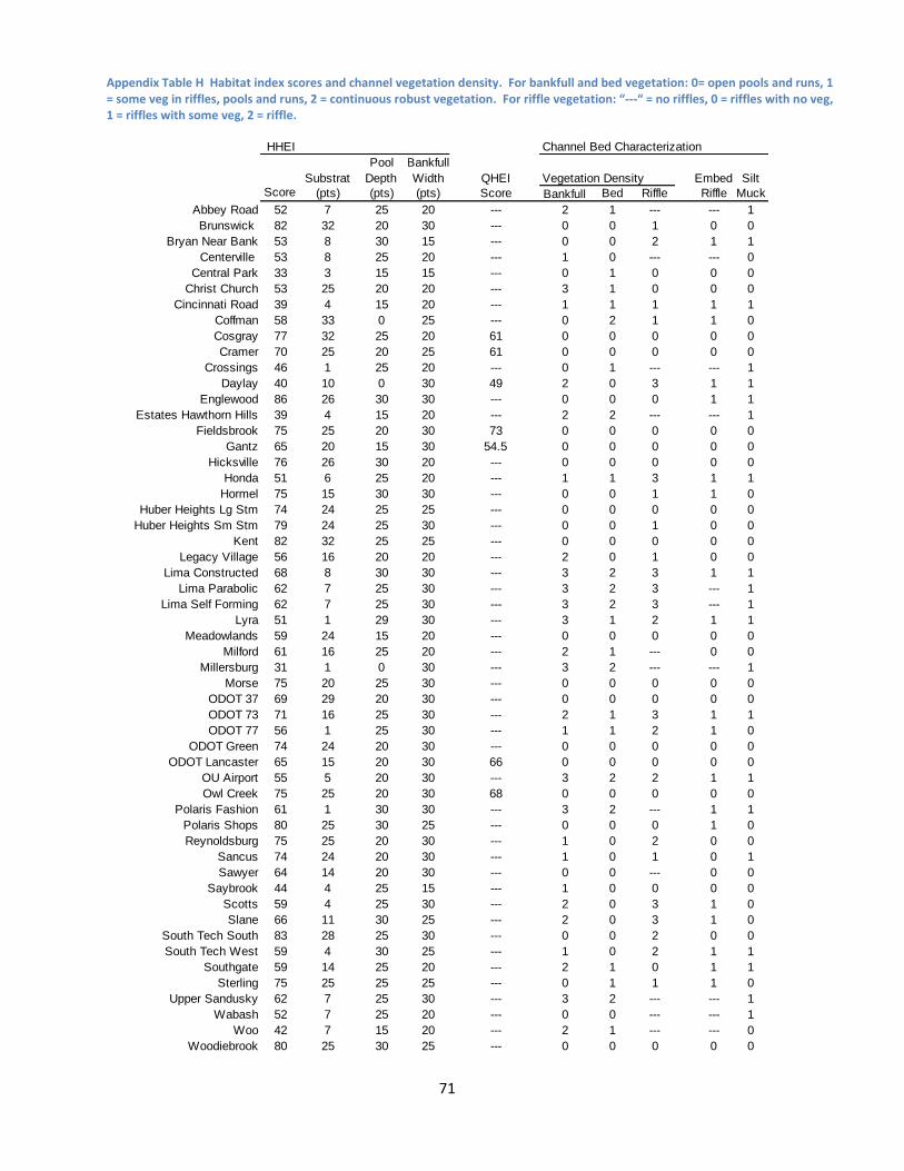
71
Appendix Table H Habitat index scores and channel vegetation density. For bankfull and bed vegetation: 0= open pools and runs, 1 = some veg in riffles, pools and runs, 2 = continuous robust vegetation. For riffle vegetation: “---“ = no riffles, 0 = riffles with no veg, 1 = riffles with some veg, 2 = riffle.
HHEI Channel Bed Characterization
Pool Bankfull
Substrat Depth Width QHEI Vegetation Density Embed SiltScore (pts) (pts) (pts) Score Bankfull Bed Riffle Riffle Muck
Abbey Road 52 7 25 20 --- 2 1 --- --- 1
Brunswick 82 32 20 30 --- 0 0 1 0 0
Bryan Near Bank 53 8 30 15 --- 0 0 2 1 1
Centerville 53 8 25 20 --- 1 0 --- --- 0
Central Park 33 3 15 15 --- 0 1 0 0 0
Christ Church 53 25 20 20 --- 3 1 0 0 0
Cincinnati Road 39 4 15 20 --- 1 1 1 1 1
Coffman 58 33 0 25 --- 0 2 1 1 0
Cosgray 77 32 25 20 61 0 0 0 0 0
Cramer 70 25 20 25 61 0 0 0 0 0
Crossings 46 1 25 20 --- 0 1 --- --- 1
Daylay 40 10 0 30 49 2 0 3 1 1
Englewood 86 26 30 30 --- 0 0 0 1 1
Estates Hawthorn Hills 39 4 15 20 --- 2 2 --- --- 1
Fieldsbrook 75 25 20 30 73 0 0 0 0 0
Gantz 65 20 15 30 54.5 0 0 0 0 0
Hicksville 76 26 30 20 --- 0 0 0 0 0
Honda 51 6 25 20 --- 1 1 3 1 1
Hormel 75 15 30 30 --- 0 0 1 1 0
Huber Heights Lg Stm 74 24 25 25 --- 0 0 0 0 0
Huber Heights Sm Stm 79 24 25 30 --- 0 0 1 0 0
Kent 82 32 25 25 --- 0 0 0 0 0
Legacy Village 56 16 20 20 --- 2 0 1 0 0
Lima Constructed 68 8 30 30 --- 3 2 3 1 1
Lima Parabolic 62 7 25 30 --- 3 2 3 --- 1
Lima Self Forming 62 7 25 30 --- 3 2 3 --- 1
Lyra 51 1 29 30 --- 3 1 2 1 1
Meadowlands 59 24 15 20 --- 0 0 0 0 0
Milford 61 16 25 20 --- 2 1 --- 0 0
Millersburg 31 1 0 30 --- 3 2 --- --- 1
Morse 75 20 25 30 --- 0 0 0 0 0
ODOT 37 69 29 20 30 --- 0 0 0 0 0
ODOT 73 71 16 25 30 --- 2 1 3 1 1
ODOT 77 56 1 25 30 --- 1 1 2 1 0
ODOT Green 74 24 20 30 --- 0 0 0 0 0
ODOT Lancaster 65 15 20 30 66 0 0 0 0 0
OU Airport 55 5 20 30 --- 3 2 2 1 1
Owl Creek 75 25 20 30 68 0 0 0 0 0
Polaris Fashion 61 1 30 30 --- 3 2 --- 1 1
Polaris Shops 80 25 30 25 --- 0 0 0 1 0
Reynoldsburg 75 25 20 30 --- 1 0 2 0 0
Sancus 74 24 20 30 --- 1 0 1 0 1
Sawyer 64 14 20 30 --- 0 0 --- 0 0
Saybrook 44 4 25 15 --- 1 0 0 0 0
Scotts 59 4 25 30 --- 2 0 3 1 0
Slane 66 11 30 25 --- 2 0 3 1 0
South Tech South 83 28 25 30 --- 0 0 2 0 0
South Tech West 59 4 30 25 --- 1 0 2 1 1
Southgate 59 14 25 20 --- 2 1 0 1 1
Sterling 75 25 25 25 --- 0 1 1 1 0
Upper Sandusky 62 7 25 30 --- 3 2 --- --- 1
Wabash 52 7 25 20 --- 0 0 --- --- 1
Woo 42 7 15 20 --- 2 1 --- --- 0
Woodiebrook 80 25 30 25 --- 0 0 0 0 0