DOWNHOLE ENTHALPY MEASUREMENT IN … ENTHALPY MEASUREMENT IN GEOTHERMAL WELLS Egill Juliusson,...

PROCEEDINGS, Thirty-First Workshop on Geothermal Reservoir Engineering Stanford University, Stanford, California, January 30-February 1, 2006 SGP-TR-179

DOWNHOLE ENTHALPY MEASUREMENT IN GEOTHERMAL WELLS

Egill Juliusson, Roland N. Horne

Stanford University, Department of Petroleum Engineering Green Earth Sciences Building, 367 Panama Street

Stanford, CA, 49305-2220, USA e-mail: [email protected]

ABSTRACT

Advances have been made in the ongoing research to find a way to measure enthalpy downhole in geothermal wells. The project has thus far revolved around determining applicable ways to determine the presence of air vs. water, which could ultimately lead to an estimate of the void fraction and enthalpy. The measurement principles tested have been based on temperature, resistivity and optical transmissivity. Successful results utilizing cross correlation techniques have lead to quite accurate estimates of bubble velocity using both resistivity measurements and optical measurements. However, so far, temperature measurements have not proven to be successful. Preliminary testing based on resistivity properties of two phase flow for determination of void fraction has begun. Future work includes deriving correlations between void fraction and resistivity using a new electrode design which looks outward from an in-situ probe into the well bore. Finally, the possibility of cross correlating the signal from two such electrode setups (spaced a known distance apart) is being investigated in the hope of obtaining the vapor velocity.

INTRODUCTION

Downhole measurement of enthalpy in geothermal wells is of interest to the industry for several reasons. For example, the enthalpy profile of a well could provide useful additional data for constraining reservoir models by history matching and reservoir performance monitoring. Additionally abrupt changes in the profile would help reveal fractures and quantify the power output from each fracture directly. The project is very challenging due to the problem of measuring of two phase flow rates over a range of flow regimes. It is further complicated by the fact that the measurement must be done in-situ and the sensor must be able to function at temperatures up to 350 °C. At this temperature, most electronics will

fail. Hence, either a mechanical solution must be found or the electronics must be specially designed to survive the downhole environment. Successful applications have been designed for temperature, pressure and spinner measurements, where the electronics are contained in a vacuum flask and thereby isolated from the heat. However, the spinner measurements have not proven to give a very accurate flow description. Recent developments of optical fiber technology have also brought new ways to measure pressure and temperature downhole but a means to quantify the additional flow parameters needed to directly determine the enthalpy is not available. The enthalpy rate, as referred to in this paper, is defined as the amount of internal energy (U) plus the compressive energy (PV) passing through a section of the wellbore over a unit time. Thus, a direct measurement of the enthalpy rate of a two phase flow would require knowledge of the temperature, void fraction and flow rate of both phases. In practice it has proven difficult to develop sensors that can accurately predict the flow rates of each phase in a two phase flow over all flow regimes. Hence, the focus of this research project has been to look at ways to measure the void fraction and flow rate of one of the phases, over a limited range of flow regimes. After all, an estimate of these two parameters, in conjunction with pressure and temperature measurements and the total flow rate at the well head would be sufficient to define a unique enthalpy profile.

THEORY

Enthalpy is a property of a system that can be defined (per unit mass) as:

Pvuh += [kJ/kg] (1)

Here u is the internal energy of the system per unit mass, P is the pressure and v is the specific volume. Enthalpy is a thermodynamic property and can therefore be found from P-vs.-T relations given two of the parameters P, v and T. For flowing fluids it is

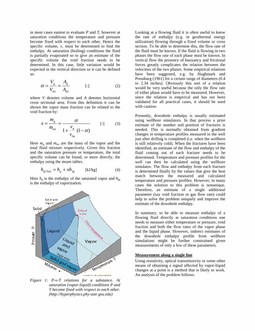
in most cases easiest to evaluate P and T, however at saturation conditions the temperature and pressure become fixed with respect to each other. Hence the specific volume, v, must be determined to find the enthalpy. At saturation (boiling) conditions the fluid is partially evaporated so to give an estimate of the specific volume the void fraction needs to be determined. In this case, little variation would be expected in the vertical direction so it can be defined as:

tot

g

tot

g

A

A

V

V==α [-] (2)

where V denotes volume and A denotes horizontal cross sectional area. From this definition it can be shown the vapor mass fraction can be related to the void fraction by:

)1(1 α

α

−+==

liq

gtot

g

v

vm

mx [-] (3)

Here mg and mtot are the mass of the vapor and the total fluid mixture respectively. Given this fraction and the saturation pressure or temperature, the total specific volume can be found, or more directly, the enthalpy using the steam tables.

fggTsat xhhh +=@ [kJ/kg] (4)

Here hg is the enthalpy of the saturated vapor and hfg is the enthalpy of vaporization.

Figure 1: P-v-T relations for a substance. At

saturation (vapor-liquid) conditions P and T become fixed with respect to each other. (http://hyperphysics.phy-astr.gsu.edu)

Looking at a flowing fluid it is often useful to know the rate of enthalpy (e.g. in geothermal energy utilization) flowing through a fixed volume or cross section. To be able to determine this, the flow rate of the fluid must be known. If the fluid is flowing in two phases the flow rate of each phase must be known. In vertical flow the presence of buoyancy and frictional forces greatly complicates the relation between the velocities of the two phases. Some empirical relations have been suggested, e.g. by Hughmark and Pressburg (1961) for a certain range of diameters (0.4 to 2.34 inches). Obviously this sort of a relation would be very useful because the only the flow rate of either phase would have to be measured. However, since the relation is empirical and has not been validated for all practical cases, it should be used with caution. Presently, downhole enthalpy is usually estimated using wellbore simulators. In that process a prior estimate of the number and position of fractures is needed. This is normally obtained from gradient changes in temperature profiles measured in the well just after drilling is completed (i.e. when the wellbore is still relatively cold). When the fractures have been identified, an estimate of the flow and enthalpy of the fluid coming out of each fracture needs to be determined. Temperature and pressure profiles for the well can then be calculated using the wellbore simulator. The flow and enthalpy from each fracture is determined finally by the values that give the best match between the measured and calculated temperature and pressure profiles. However, in many cases the solution to this problem is nonunique. Therefore, an estimate of a single additional parameter (say void fraction or gas flow rate) could help to solve the problem uniquely and improve the estimate of the downhole enthalpy. In summary, to be able to measure enthalpy of a flowing fluid directly at saturation conditions one needs to measure either temperature or pressure, void fraction and both the flow rates of the vapor phase and the liquid phase. However, indirect estimates of the downhole enthalpy profile from wellbore simulations might be further constrained given measurements of only a few of these parameters.

Measurement along a single line Using resistivity, optical transmissivity or some other means of obtaining a signal affected by vapor-liquid changes at a point is a method that is likely to work. An analysis of the problem follows.

Figure 2: Cross section of pipe with vapor-liquid

flow. A resistivity measurement (or equivalent) is being taken at multiple points across the “measured line”.

The goal is to find the enthalpy rate i.e. energy passing through the cross sectional area

∑+=i

gif AAA [m2] (5)

(here Af is the area occupied by liquid and Agi is the area occupied by vapor bubble i) per time unit. The enthalpy of the saturated vapor (hg) and liquid (hf) can be found from the steam tables and given the flow velocity (u) of each phase the flow rate can be found from

AuAuq gi

gigg α== ∑ [m3/s] (6)

Au

AAuq

f

igiff

)1( α−=

⎟⎠

⎞⎜⎝

⎛ −= ∑ [m3/s] (7)

Then the total enthalpy rate for each phase can be found as

g

ggg v

qhH =& [J/s] (8)

f

fff v

qhH =& [J/s] (eq .9)

Here the specific volumes vg and vf can be obtained from the steam tables, and the total enthalpy of the mixture is:

f

ff

g

gg

fg

v

uAh

v

uAh

HHH

)1( αα −+=

+= &&&

[J/s] (10)

So the average fraction of the cross section occupied by steam needs to be determined, i.e. the void fraction

A

Ai

gi∑=α [-] (11)

Suppose a measurement is taken at multiple points along a line across a cross section of a pipe (Figure 2). Assuming the bubbles will flow randomly through the cross section of the pipe, the fraction of the line that is occupied by vapor, averaged over time, would give the average fraction of steam going through the whole cross section (Figure 3).

Figure 3: The measured line, averaged over time,

will likely form a symmetric distribution of vapor concentration. Lighter blue means more time on average occupied by vapor.

If B(r) is defined as the time the measurement line is occupied by vapor at radius r divided by the total time the measurement is taken then as time goes by B(r) will form a smooth symmetric distribution. Integrating the distribution, B(r), over the cross

sectional area gives the area occupied by steam on average, Ag,av and dividing by the total area gives the formula for the average void fraction

∫

∫

=

==

2/

02

2

2/

0,

)(8

4/

)(2

D

D

avg

drrrBD

D

drrrB

A

A

ππ

α [-] (12)

This shows that it would suffice to measure the presence of gas vs. water at a few points along a single line across the pipe diameter to determine the average void fraction.

EXPERIMENTS

Experiments testing the applicability of using temperature, resistivity and optical sensors were carried out in a simple setup of segmented air-water flow. Temperature was measured with a fast response (~20 ms) thermocouple (type: Omega 5TC-TT-T-40-36). A resistivity sensor was made by fixing two electrodes (open ended wires) a small distance apart (~2 mm). When the sensor was placed in the flow path the voltage drop across the electrodes would depend on the resistance of the surrounding medium. The optical sensor consisted of a phototransistor on one side of the tube and a light source on the opposite side. When a bubble passed, less light passed through and the resistance of the phototransistor increased. A schematic diagram of the circuit for the resistivity and optical sensors is shown in Figure 4. A schematic diagram of the experiment is shown in Figure 5. The figure shows how a mixed air-water flow (flowing vertically upwards) passes three types of sensors, at three different spots. At spots 1 and 2

we have an optical, temperature and resistivity measurement. At spot 3 we only have a temperature measurement. After the fluid mixture passed the sensors it was separated and the quantity of each phase was measured over a specific time interval to find the individual flow rates. This basic configuation was used with flow tubes of two different sizes. First a 1/8 in. diameter brass tube was used, in which segmented air-water flow could be assumed. A 1 in. tube in which a single fully formed bubble would flow through the cross section was later used. In this case the length of the tube compared to the sensor spacing was too short such that the bubble pattern had changed significantly on the way from one sensor to the other. Therefore the results in the 1 in. tube were used more qualitatively to asses the applicability of using one sensor type vs. the other. The data acquisition program was developed in LabView. The program logged all seven sensors simultaneously at 1 kHz and wrote the results to a scaled binary output file. The output file was then decoded in Matlab for further data processing. Each test run was logged for approximately 10 seconds. There were some problems with 60 Hz electrical noise in the measurements. Grounding the power source made a particularly large improvement in that respect but nevertheless the noise in the temperature signal was never reduced to less than ±0.5°C. Moreover, there were some issues regarding cross talk between the two resistivity sensors i.e. a fluctuation in the signal from sensor 1 was sometimes seen at the same time in sensor 2. This phenomena is discussed further in the next section.

Figure 4: A circuit diagram for the phototransistor and resistivity sensors. As the diagram shows, a single 12V DC

source drives the whole circuit. When an air bubble passes one of the sensors, the resistance of the electrode/phototransistor changes, hence a different voltage drop is measured across the reference resistor connected to the terminal block.

Figure 5: A schematic of the experiment setup. A vertical air-water flow is investigated by three types of sensors. A

simple flow meter then measures the flow rate of each phase separately.

DATA ANALYSIS

Bubble velocity In order to directly calculate the enthalpy rate of a two-phase flow, the steam and liquid average velocities need to be determined. A part of that would be to find the velocity of the steam bubble as it traveled up the borehole. Using the signals obtained from two sensors, spaced a known distance apart, this bubble velocity could be inferred. Given the distance between the sensors, L, the mean bubble velocity would be

tt

Lv = . [m/s] (13)

In the case of our experiment, the time, tt, it took the bubble to travel from one sensor to the other, i.e. the time shift between the patterns measured by each sensor is what needed to be found. For slow and dispersed bubble flow (Figure 6) this could easily be seen from a quick look at the signals but when the bubble flow became more rapid (Figures 7 and 8) the pattern in the signal became harder to discern.

Figure 6: Signals obtained from the resistivity and

optical sensors at two different locations The bubble flow was relatively slow and dispersed. Hence a bubble pattern is clearly detectable and the time shift can be estimated visually. This will be referred to as Pilot test 2.

1.1 1.2 1.3 1.4 1.6 1.7 1.8 1.9 2 10.1

10.2

10.3

10.4Resistivity1

1.1 1.2 1.3 1.4 1.6 1.7 1.8 1.9 2 0.4 0.5 0.6 Phototrans1

1.1 1.2 1.3 1.4 1.5 1.6 1.7 1.8 1.9 2 9.2 9.4 9.6 9.8 10 Resistivity2

1.1 1.2 1.3 1.4 1.5 1.6 1.7 1.8 1.9 2 0.220.240.260.280.3 0.32

Phototrans2

Time [s]

Actual Signal Fourier Filtering




Figure 7: Signals from the resistivity and optical

sensors. As seen by comparison to the signals in Figure 6, the bubble flow is getting more rapid and the pattern is now harder to discern. This will be referred to as Pilot test 1.

Figure 8: Here we see the response from the same

sensors as in used previously but now the bubble flow is much more rapid. The bubble pattern is very hard to discern. This will be referred to as Pilot test 3.

Cross correlations A relatively simple but robust method to find the time shift in the signals was to calculate the cross-correlation function (XCF) between the two signals. The cross-correlation function is a function of the correlation coefficient between the two signals, where one of the signals has been shifted in time. The time at which the XCF has its maximum value then corresponds to the time shift between the two signals. The XCF is defined as follows:

∫ −−−= tott

totxy dtytyxtx

tR

0))()()((

1)( ττ (14)

Here x and y are the two signals, x and y are the signal averages over the entire measurement interval, ttot, and τ is the time shift. This method is commonly used in flow metering technology and has worked well to measure concentration signals that are

stochastic in nature. This is most often the case in turbulent two-phase flows. The method was tested on each of the signals and the results for Pilot test 2 and 3 are shown in Figures 9 and 10.

-0.5 0 0.5-0.3

-0.2

-0.1

0

0.1

0.2

0.3

0.4

0.5

0.6

0.7

Time shift = 0.283 [s]

Time increments-τ [s]

Sam

ple

cros

s-co

rrel

atio

n


Figure 9: This graph of Rxy(τ) for each sensor type

(test corresponding to Figure 6) shows a clear maximum at τ ≈ 0.28 s. Phototransistor data are in green and resistance data are in magenta. This is to verify that the cross-correlation method works.

Figure 10: This graph of Rxy(τ) for each sensor type

(test corresponding to Figure 8) shows a clear minimum at τ ≈ 0.11 s. The erroneous value of -0.001 s is predicted by the resistivity sensor because of crosstalk between the electrodes.

It was shown that the time shift could be found surprisingly clearly and accurately by this method. The only case in which the method broke down, was when measuring the rapid bubble flow using the resistivity sensors. In that case the maximum correlation was found for time shift τ ≈ 0. This erroneous result was introduced because of crosstalk between the two electrode sensors. Ways to resolve the problem are discussed in a later section.

0 0.1 0.2 0.3 0.4 0.5 0.6 0.7 0.8 0.9 1 9.6

9.8

10 Resistivity1


0 0.1 0.2 0.3 0.4 0.5 0.6 0.7 0.8 0.9 1 0.4

0.5

0.6

Phototrans1


0 0.1 0.2 0.3 0.4 0.5 0.6 0.7 0.8 0.9 1 9.2

9.4

9.6

9.8 Resistivity2


0 0.1 0.2 0.3 0.4 0.5 0.6 0.7 0.8 0.9 1 0.2

0.25

0.3Phototrans2


5.1 5.2 5.3 5.4 5.5 5.6 5.7 5.8 5.9 6 9.6 9.8 10 10.2

5.1 5.2 5.3 5.4 5.5 5.6 5.7 5.8 5.9 6 0.3 0.4 0.5

Phototrans1

5.1 5.2 5.3 5.4 5.5 5.6 5.7 5.8 5.9 6 9.4 9.6 9.8 10 10.2Resistivity2

5.1 5.2 5.3 5.4 5.5 5.6 5.7 5.8 5.9 6 0.15

0.2 0.25

Phototrans2

Time [s]





Resistivity1

Time [s]

Scaled signal differences A second method to determine the time shift was also devised, and is presented here to give comparison to the results obtained from the cross-correlation function. The basic idea was to find the time shift that gives the minimum difference when one signal was subtracted from the other. Since the signals were not necessarily at the same scale they had to be scaled by the ratio of the averages of the two signals, before taking the difference. The time shift between the signals was the value that minimized this quantity. More compactly, the goal was to find τ subject to:

⎪⎭

⎪⎬⎫

⎪⎩

⎪⎨⎧

+−=∆ )()()(min ττ tyy

xtxxy (15)

Since the data sets at hand were usually not very large it was easy to calculate the difference ∆xy as a function of τ on some reasonable interval and find the time shift corresponding to the minimum value in that dataset. Figures 11 and 12 show ∆xy(τ), calculated from the signals in Pilot tests 1 and 3. The results of this method were very consistent with those from the cross-correlation technique. In these two cases it seems that this method is more consistent, since the variability between the time shifts predicted by each sensor is smaller.

0 0.2 0.4 0.6 0.8 1 1.2 1.4 1.6 1.8 20.03

0.04

0.05

0.06

0.07

0.08

0.09

0.1

0.11

0.12


Time increments [s]

Mea

n di

ffer

ence

bet

wee

n si

gnal

s


Figure 11: This graph of ∆xy(τ) for each sensor type

(test corresponding to Figure 7) shows a clear minimum at τ ≈ 0.18 s. Phototransistor data are in green and resisivity data are in blue.

0 0.2 0.4 0.6 0.8 1 1.2 1.4 1.6 1.8 20.04

0.06

0.08

0.1

0.12

0.14

0.16

0.18


Time increments [s]

Mea

n di

ffer

ence

bet

wee

n si

gnal

s



Correct time shift value

Erroneous time shift value

Figure 12: This graph of ∆xy(τ) for each sensor type

(test corresponding to Figure 8) shows a clear minimum at τ ≈ 0.11 s. The erroneous value of 0.001 s is again predicted by the resistivity sensor because of crosstalk between the electrodes.

Void fraction and bubble geometry One of the more important quantities that one would like to measure in downhole wellbore flow is the void fraction. To that end, estimating the bubble frequencies and being able to count the bubbles becomes important. This proved nontrivial using the electrical resistivity measurements, due to a low signal-to-noise ratio and crosstalk effects. This section introduces some of the problems involved and the methods that were used for the analysis. Since the experiment dealt with segmented flow the bubble geometry could be modeled as a cylinder of diameter equal to the tubing diameter and length Lb,i which could be calculated as

ibib vtL ,, = [m] (16)

where v is the bubble velocity (as obtained earlier) and the tb,i is the time it took bubble number i to pass the sensor. Another property arising from the fact that the flow was segmented was that the water and air flow velocities were the same, and therefore the void fraction could be calculated as

tot

iib

tot

iib

tot

iib

t

t

vL

vL

AL

AL

∑

∑∑

=

==

.

,,

/

/α

[-] (17)

where Ltot is the total length of fluid (air and water) that passed through the measured section and all other quantities are as defined earlier.

Figure 13: A simplified model of vertical segmented

flow. By assuming that the water and air velocities are the same, the void fraction can be calculated as the ratio between the total time the sensor measures the presence of air and the total measurement time.

Given these assumptions, the total time that bubbles were present was all that was needed to calculate the void fraction. However, this quantity was not easily determined from the measurements because of the relatively slow response time of the sensors. Moreover, in the case of the resistivity measurements, the low signal-to-noise ratio and the crosstalk complicated the analysis still further. Two basic methods were investigated to infer consistent estimates of the void fraction between all four sensors.

Threshold from histogram In the first method a histogram of the measurement points was made and some intermediate value that could correspond to a transition value between air and water measurements was to be determined. This intermediate value had to be somewhere between the two peaks corresponding to measurement values for air and water as shown in Figure 14 (data taken from Pilot test 1). The threshold value for transition between air and water measurements was not defined clearly from the histogram for the phototransistor measurements and the situation did not improve by looking at the

resistivity measurements (Figure 15). Thus, this method was abandoned for the time being, keeping in mind that it might become feasible if the response time and accuracy of the sensors could be improved.

Figure 14: A histogram of measurements made with

phototransistor 1 at an intermediate flow rate. It is not clear where the threshold value for transition between air and water measurements lies.

Figure 15: A histogram of measurements made with

resistivity sensor 1 at an intermediate flow rate. It is hard to determine which signals correspond to presence of air and where to put the threshold value for the transition between the fluids.

Moving average threshold The second method investigated was to draw a threshold line that varied in time based on local variations in the signal. One advantage of using a method like this was that it might be useful in situations if the properties of the fluid were changing in time (e.g. if the measurement tool is being lowered downhole, the resistivity of the fluid would vary with depth and time). The threshold line was drawn as a one second moving average (note that the actual signal had also been filtered to remove the 60 Hz electrical noise). Figure 16 illustrates data from the phototransistor and Figure 17 has data from the resistivity sensor (data taken from Pilot test 1).

0.25 0.3 0.35 0.4 0.45 0.5 0.55 0.6 0.65 0.7 0

500

1000

1500

2000

2500

3000

Sensor measurement value [V]

Fre

quen

cy

Values corresponding to presence of water

Values corresponding to presence of air

Threshold value?

9 9.2 9.4 9.6 9.8 10 10.2 0

200

400

600

800

1000

1200

1400

1600

1800

2000

Sensor measurement value [V]

Fre

qenc

y

Values corresponding to presence of air?

Threshold value?

Values corresponding to presence of water

Figure 16: A moving average threshold used to

determine whether the signal from a phototransistor corresponds to air or water.

Figure 17: A moving average threshold used to

determine whether the signal from resistivity sensor corresponds to air or water.

As indicated by Figures 16 and 17, a fairly accurate bulk estimate of the presence of bubbles was obtained. The bubble signals from the two sensors showed a relatively good correlation and the calculated void fraction was 29.3% as calculated from the phototransistor 1 measurement but 31.1% using the resistivity sensor 1. Note also that because of the electrical noise in the resistivity measurement, it tended to estimate more frequent and smaller bubbles than did the phototransistor. The moving average threshold method works fairly well as long as the void fraction is in the intermediate ranges (say 20-80%), but as the limit of pure water or pure air is approached the method will cease to work because the moving average threshold will move too close to the signal of the dominant fluid. Hence, an underestimate of the dominant fluid is obtained. Tables 1 to 3 summarize estimates of bubble velocity, average bubble length, void fraction and the number of bubbles counted over the measurement period for each of the three Pilot tests. Table 4 shows the measured flow rates and flow rate ratios measured using the simple flow meter. Given the aforementioned assumptions for segmented flow, the ratio Qair/Qtot should equal the void fraction and hence the two values could be compared to get an estimate of the accuracy of these calculations. Some caution should be taken in the comparison since the uncertainty in the measurements from the flow meter was rather large.

Table 1: Summarized results for calculated bubble flow properties from Pilot test 1. Sensor: Resistivity1 Resistivity2 Phototrans1 Phototrans2 STDBbl Velocity [m/s]: 0.287 0.287 0.281 0.281 0.0038Avg Bbl Length [mm]: 6.5 5.4 9 8.6 1.7Void Fraction: 31.1% 27.6% 29.3% 30.8% 2%Number of Bbls: 279 296 184 203 55P

ilot te

st 1

Table 2: Summarized results for calculated bubble flow properties from Pilot test 2. Sensor: Resistivity1 Resistivity2 Phototrans1 Phototrans2 STDBbl Velocity [m/s]: 0.181 0.181 0.179 0.179 0.0008Avg Bbl Length [mm]: 6.4 4.8 9.3 8.2 2.0Void Fraction: 27.4% 24.8% 20.1% 20.1% 4%Number of Bbls: 143 173 71 82 49P

ilot te

st 2

Table 3: Summarized results for calculated bubble flow properties from Pilot test 3. Sensor: Resistivity1 Resistivity2 Phototrans1 Phototrans2 STDBbl Velocity [m/s]: 0.467 0.467 0.467 0.467 0.0000Avg Bbl Length [mm]: 8.2 9.2 12.8 10.3 2.0Void Fraction: 35.9% 49.6% 58.2% 54.9% 10%Number of Bbls: 378 464 392 459 45P

ilot te

st 3

3 3.1 3.2 3.3 3.4 3.5 3.6 3.7 3.8 3.9 4 0.3 0.4 0.5 0.6 0.7

Time [s]

Sig

nal

Moving average threshold for phototransistor 1 in segmented bubble flow

3 3.1 3.2 3.3 3.4 3.5 3.6 3.7 3.8 3.9 4 0

0.2 0.4 0.6 0.8

1

Time [s]

Wat

er(0

) or

Air(

1)

Air-water distribution

Actual signal (filtered) 1 second moving average

3 3.1 3.2 3.3 3.4 3.5 3.6 3.7 3.8 3.9 4 9.7 9.8 9.9 10

10.1

Time [s]

Sig

nal

Moving average threshold for resitivity sensor 1 in segmented bubble flow

3 3.1 3.2 3.3 3.4 3.5 3.6 3.7 3.8 3.9 4 0

0.2 0.4 0.6 0.8

1

Time [s]

Wat

er(0

) or

Air(

1)

Air-water distirbution

Actual signal (filtered) 1 second moving average

Table 4: Measurement results from the simple flow meter. The ratio Qair/Qtot can be compared to the void fractions reported in Tables 1 to 3. Note the relatively large uncertainty in the measurements made by the flow meter.

As expected the moving average threshold method seemed to work fairly well when the void fraction was at an intermediate value. This was seen in Pilot test 2. In Pilot test 1 the void fraction had become too low for a proper estimate to be made by this method and an underestimate of the water (the dominant fluid) was seen. In the case of Pilot test 3, an underestimate of air was seen, which was not predicted by this simple model of the segmented flow, but this could perhaps be explained by turbulence and vibrational effects that the flow had on the electrode. Electrical noise and crosstalk may also have played a role here.

Crosstalk In the case of the resistivity measurements a crosstalk effect was seen between the two sensor readings. This means for example, that sometimes when a bubble passed the resistivity sensor at spot 1, a signal change was seen in the resistivity measurement at spot 2 also. This was very clear e.g. in the signal seen around time 7.7s in Figure 6. In an attempt to explain this behavior one could propose that the anode of electrode 1 and the cathode of electrode 2 were connected through the water and formed another electrode. Let the resistance across this electrode be denoted by Re12. Then the measured voltage drop in circuit 2 could be calculated as

1

1222 )

11( −+−=

eeR

RRIVV [V] (17)

where Re2 is the voltage drop across electrode 2 and V

= 12V is the total voltage supplied to the circuit. When a bubble passes electrode 1 the connection between electrodes 1 and 2 weakens and Re12 goes up. According to equation 13 this leads to a lower value of VR2. The change in the signal because of this disturbance would be much smaller than the change in the signal if the bubble were passing at spot 2 because Re12 >> Re2

A similar relation should exist the other way around, between electrodes 2 and 1, but it was not seen as strongly, perhaps because the current could not travel as easily upstream, i.e. Re12 was not equal to Re21.

This could be because of a second bubble, traveling in between the sensors, that impeded the current. This explanation is perhaps not completely satisfactory and using separate power supplies for each sensor has been suggested by specialists that have developed a similar technology at the Schlumberger Experimental Facilities in Cambridge, UK. Alternative ways to deal with the crosstalk, i.e. signal processing methods, were also investigated. The way that gave the best results was to subtract the lagging signal (y) from the leading signal (x) and then cross correlate z = x - y to y. This way, the erroneous part of the signal (resulting from crosstalk) could be subtracted out of the leading signal and the peak in Rxy(τ) at τ≈0 was eliminated (Figure 18).

-0.5 0 0.5-0.4

-0.3

-0.2

-0.1

0

0.1

0.2

0.3

0.4


Time increments-τ [s]

Sam

ple

cros

s-co

rrel

atio

n


Figure 18: The cross-correlation between the lagging

signal (y) and the difference between the leading and the lagging signal (z=x-y) provides an appropriate estimate of the time shift.

FUTURE WORK

Full-size application design Some preliminary measurements have been made in a full-sized artificial well. The artificial well consists of a 6 in. diameter plexiglass tube which has adjustable air and water flow. A flow mixer is at the bottom of the tube so the flow will be homogeneous. Preliminary measurements with an electrode design

which is sketched roughly in Figure 19 have yielded results that show generally increased resistance as the amount of air is increased but a flow meter for the air is yet to be obtained.

Figure 19: Shown is a cross section of a wellbore

with an in-situ probe that consists of an electrode made of two brass plates (brown). The resistance across the electrode depends on the void fraction of the welbore flow.

As soon as the air flow rate can be measured, the reference void fraction can be calculated and correlations for the relation between resistance and void fraction can be made. To obtain an additional reference for the void fraction, a manometer will be attached to the side of the artificial well and the void fraction then calculated from the weight of the air-water column.

REFERENCES

Aziz, K. and Govier, G.W.: The Flow of Complex Mixtures in Pipes, Van Nostrand Reinold Company, 1972, pages 338-339.

Boles, M.A. and Çengel, Y.A.: Thermodynamics, An Engineering Approach, McGraw-Hill Companies, Inc., 2002.

Chen, C.Y., Horne, R.N., Li, K., and Villaluz, A.L.: “Quarterly Report for Contract DE-FG36-02ID14418, Stanford Geothermal Program, April-June 2004,” Stanford University, 2004, page 4.

Chen, C.Y., Dastan, A., Juliusson, E., Horne, R.N., Li, K., Stacey, R.W. and Villaluz, A.L.: “Quarterly Report for Contract DE-FG36-02ID14418, Stanford Geothermal Program, January-March 2005,” Stanford University, 2005.

Cheremisinoff, P.N., Cheremisinoff, N.P.: “Flow Measurement for Engineers and Scientists”, Marcel Dekker, inc, 1988. p. 101-130

Crow, C.T., Sommerfeld, M., Tsujinaka, Y., “Multiphase Flows With Droplets and Particles”, CRC Press, 1997. p. 309

Hughmark, G.A., and Pressburg, B.S.:"Holdup and pressure drop with gas-liquid flow in a vertical pipe," A.I.Ch.E. Journal, Vol. 7; page 677 (1961).

Partin, J.K., Davidson, J.R., Sponsler, E.N. and Mines, G.L.: “Deployment of an Optical Steam Quality Monitor in a Steam Turbine Inlet Line,” presented at the Geothermal Resource Council 2004 annual meeting, August 29- September 1, 2004, Indian Wells, California, USA; GRC Trans. 28 (2003).

Spielman, P.: "Continuous Enthalpy Measurement of Two-Phase Flow form a Geothermal Well," presented at the Geothermal Resource Council 2003 annual meeting, October 12-15, 2003, Morelia, Mexico; GRC Trans. 27 (2003).

DOWNHOLE ENTHALPY MEASUREMENT IN … ENTHALPY MEASUREMENT IN GEOTHERMAL WELLS Egill Juliusson,...

Documents

Transcript of DOWNHOLE ENTHALPY MEASUREMENT IN … ENTHALPY MEASUREMENT IN GEOTHERMAL WELLS Egill Juliusson,...