1

Distributive conflict, economic growth and exchange rate in Brazil1

Douglas Alcantara Alencar

Frederico Gonzaga Jayme Jr

Gustavo de Britto Rocha

Abstract

The aim of this paper is to analyse the interaction among aggregate demand, real exchange rate,

productivity for the Brazilian economy, between 1960 and 2011. Theoretical elements suggest that

there is relationship between aggregate demand, real exchange rate and productivity. The novelty is

that even though if aggregate demand regime is wage-led, exchange rate devaluation can have a

positive impact on productivity. Besides, even if the demand regime is profit-led, exchange rate

devaluation can have a negative impact on productivity, thus on economic growth. Because there is

a lack in theoretical and empirical studies in relation to the interaction between the above mentioned

macroeconomic indicators and aggregate demand regime, this research tries to investigate their

dependence.

Keywords: post-Keynesian, aggregate demand, real exchange rate, productivity, real wages

1. Introduction

Following the theoretical frameworks, in which capital accumulation and economic growth are

driven by the growth of the demand (SETTERFIELD, 2003; SAWYER, 2012; SCHODER, 2014).

This central tenet does not, however, rue out the importance of supply side factors to economic

growth. This paper takes on productivity, through the Kaldor-Verdoorn effect, to analyse its

interaction with the real exchange rate and real wages for the Brazilian economy, between 1960 and

2008 (KALDOR, 1966; NAASTEPAD, 2006; STORM & NAASTEPAD, 2012).

Theoretical fundamentals pose that there is relationship between aggregate demand, real exchange

rate, productivity and real wages. The novelty of this paper is to argue that even in an aggregate

wage-led, exchange rate devaluations can have a positive impact on productivity. On the other

hand, even if the demand regime is profit-led, exchange rate devaluations can affect productivity

and, thus, economic growth, adversely.

Some authors recommend to raise labour productivity through devaluation of the real exchange rate,

since this mechanism increases prices (caused by the devaluation of real exchange rate), and real

1 We would like to thank Malcom Sawyer and Sylvia Strawa for helpful comments on an earlier version of this paper. The usual

disclaimers applies. We are grateful to CNPq –the Brazilian National Council of Scientific and Technological Development for

the financial support.

2

wages would fall in the short term, assuming sticky nominal wages. This strategy considers, a

priori, that the demand regime is profit-led. However, as pointed out by Bhaduri and Marglin

(1990), Foley and Michl (1999), Naastepad (2006), Storm and Naastepad (2007, 2012), demand

regimes can be profit-led or wage-led, which is essentially an empirical question. In a wage-led

demand regime, a real devaluation of the exchange rate can reduce aggregate demand, which

negatively impacts capital accumulation and reduces productivity by reducing real wages.

In order investigate these matters, the paper follows these steps: i) a critical assessment of the

growth regimes literature, with a particular emphasis on the matters of productivity and real

exchange rate; ii) understanding the relationship between real exchange rate, productivity and

demand growth regimes; iii) proposing a theoretical model that relates real exchange rate,

productivity and growth regime; iv) An empirical test of the interaction between real exchange rate,

productivity and growth regime.

Besides this introduction, the second section discusses the basic Post-Keynesian/Kaleckian model.

The third section considers the interaction among demand regime, productivity and real exchange

rate. Finally, the forth section presents the conclusions.

2. Economic Growth

In Solow’s classical model, in the long run, economic growth is determined exogenously by the

supply side ‘natural rate of growth’. In the Post-Keynesian approach economic growth is an

endogenous phenomenon. The foundation for the Post-Keynesian models is based on Kaldor, the

Cambridge Equation and the endogenous economic growth.2 Kaldor (1956; 1957; 1958) discusses

the technical progress function, in which the labour productivity depends on per capita capital

growth and the existence of the relationship between economic growth and the functional income

distribution. Furthermore, in the Cambridge Equation, the capital stock growth rate depends on the

propensity of capitalist saving and the current value of profit rate. The Thrift paradox shows that if

there is an increase in propensity to save, this fact will lower the levels of capacity utilization and

reduces economic growth.

Stockhammer (1999,) Bertela (2007), and Oreiro (2011) identified three generations of economic

growth models in the Post-Keynesian tradition. The first generation was developed by Kaldor

(1956; 1957; 1958), Joan Robinson (1970), Kalecki (2009), Harrod (1933), Domar (1946), and

Luigi Pasinetti (1962). The second generation was proposed by Kalecki (2009) and Steindl (1956).

2 Endogenous growth in Post Keynesian framework is different from the endogenous growth built in Romer (1986/1990). In Romer,

the growth is endogenized by human capital in a typical Cobb-Douglas function in a dialogue with the Solow growth model, in

which the technical progress is exogenous. In a Post Keynesian framework, the endogenous growth is related to a demand-led

approach in which path-dependence is central for growth.

3

Finally the third generation has been presented by Bhaduri and Marglin (1990), Marglin and

Bhaduri (1991), Dutt (1994), Skott (1989; 1994), Lima (2000) and Naastepad (2007).

In the first generation of economic growth models, the income distribution function is endogenous,

which means that the income distribution is determined at the same together with economic growth.

The determination of this relationship guarantees full level of capacity utilization.3 In this case,

economic growth in the long term is induced by investment. As a result, investment will increase if

the profit share and/or the profit rate raises.

In the second generation models, the level of capacity utilization adjusts accordingly to changes in

savings and investment, rather than through the profit share. Increase in wages will increase

capacity utilization, and thus capital growth. The income distribution function is determined by the

exogenously given mark-up level on direct costs. Therefore, this function is also exogenous.

In the third generation models, the major innovation was to consider the degree of capacity

utilization and the profit margin as distinct arguments in the investment function, rather than

combine the arguments into the investment function. In this way, there is the possibility of rising

real wages have a positive impact on rate of profit (Stockhammer 1999; Bertella, 2007; Foley &

Michl, 1999).

According to Bhaduri and Marglin (1990), an expansion of aggregate demand and, therefore, of

economic growth may, sometimes, be achieved by increasing profit and the wage share. The

reasoning behind this argument is that the increasing wage share would lead to a positive effect on

consumption, which in turn would raise again capacity utilization and increase profit rates. The

requirement for this mechanism is that the impact on capacity utilization is higher than the impact

on reduction of the profit share. The opposite effect can also occur. Furthermore, the redistribution

of income from profits to wages may have an ambiguous effect on aggregate demand and thus,

economic growth.

The second generation of economic growth models has four major distinctions from the first

generation. First, prices are influenced by direct costs of production and the degree of monopoly.

Second, the marginal costs of production are considered constant until the economy reaches full

production capacity. Third, production capacity is not fully utilized. Fourth, the investment function

depends on the profit rate and the degree of capacity utilization.4 (Bertella, 2007).

3 In the original Kaldor approach, full employment was indeed assumed, but it could be said that it was not guaranteed, and there was

an assumed adjustment mechanism on the relative movements of wages and prices.

4. Regarding the degree of capacity utilized, the discussion made by Bhaduri and Marglin (1990) had previously been made, in some

way, by other authors. For instance, Amadeo (1986) argues that, if the level of capacity utilization is endogenous, so changes in real

wages make the effect regarding to functional distribution of income (wages and profits) ambiguous. The author argues that

reductions in real wages are not sufficient for the economy have higher rates of economic growth. On the other hand, increases in real

wages may increase on the level of capacity utilization, thus increasing the rate of profit.

4

The important innovation of the approach proposed by Bhaduri and Marglin (1990) was to consider

the degree of capacity utilization and the profit margin as distinct parts in investment function.

Thus, an increase in real wages can have a positive impact in the profit rate (STOCKHAMMER

1999; BERTELLA, 2007).

Bhaduri and Marglin (1990) argue that, in a closed economy with no government, expanding

aggregate demand can be led by the increase in wage or profit share. Increasing the wage share

would cause positive impact on consumption and increase the use of capacity utilization utilization

of firms, which would increase the rate of profit. Indeed, in order to get this result, the impact on the

capacity utilization must be greater than the impact of the reduction of the profit share in income.

On the other hand, the rising share of wages in income via higher real wages may increase the cost

of production, reducing profits, which could reduce investment and thus aggregate demand. The

redistribution of income from profits to wages, or otherwise, may have an ambiguous effect on

aggregate demand and economic growth.

3. Economic Growth, Real Exchange Rate and Aggregate Demand

Consider the following equation in growth rates:

𝑦 = 𝑐 + 𝑖 + 𝑥 − 𝑚 (1)

where 𝑦 is the output, 𝑐 the aggregate consumption; 𝑖 the aggregate investment; 𝑥 the exports; and

𝑚 the imports These variables are measured at constant prices.

Defining 𝜔 = (𝑊/𝑃)𝜆−1 = 𝑤𝜆−1 as real cost of labour per unit of output (TAYLOR, 1991), where

𝜔 is defined as the wage share, 𝑊 the nominal wage, 𝑃 the price, and finally 𝜆 the productivity.

The labour cost per unit of output in growth rate can be obtained from:

𝑣 = �̂� − �̂� (2)

Where 𝑣 represents the growth rate of labour cost per unit of output, �̂� growth rate of the real wage,

and �̂� growth rate of productivity. If �̂� is greater than �̂�, 𝑣 will also grow. This means that the

growth rate of 𝑣 will affect the income distribution from profits towards wage. The opposite also

occurs if �̂� is growing faster than �̂�. In this case, there will be income redistribution from wages to

profits (NAASTEPAD & STORM, 2007).

Defining real profit share:

𝜋 = 1 − 𝜔 (3)

5

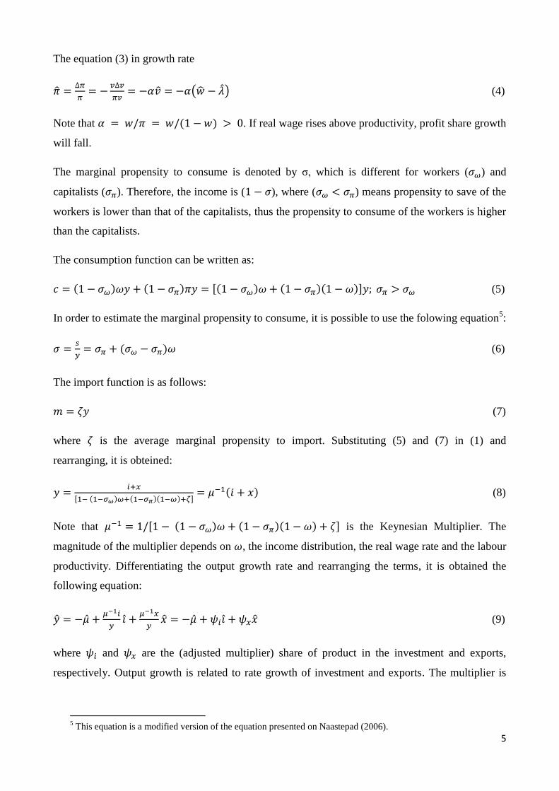
The equation (3) in growth rate

�̂� =∆𝜋

𝜋= −

𝑣∆𝑣

𝜋𝑣= −𝛼𝑣 = −𝛼(�̂� − �̂�) (4)

Note that 𝛼 = 𝑤/𝜋 = 𝑤/(1 − 𝑤) > 0. If real wage rises above productivity, profit share growth

will fall.

The marginal propensity to consume is denoted by σ, which is different for workers (𝜎𝜔) and

capitalists (𝜎𝜋). Therefore, the income is (1 − 𝜎), where (𝜎𝜔 < 𝜎𝜋) means propensity to save of the

workers is lower than that of the capitalists, thus the propensity to consume of the workers is higher

than the capitalists.

The consumption function can be written as:

𝑐 = (1 − 𝜎𝜔)𝜔𝑦 + (1 − 𝜎𝜋)𝜋𝑦 = [(1 − 𝜎𝜔)𝜔 + (1 − 𝜎𝜋)(1 − 𝜔)]𝑦; 𝜎𝜋 > 𝜎𝜔 (5)

In order to estimate the marginal propensity to consume, it is possible to use the folowing equation5:

𝜎 =𝑠

𝑦= 𝜎𝜋 + (𝜎𝜔 − 𝜎𝜋)𝜔 (6)

The import function is as follows:

𝑚 = 𝜁𝑦 (7)

where 𝜁 is the average marginal propensity to import. Substituting (5) and (7) in (1) and

rearranging, it is obteined:

𝑦 =𝑖+𝑥

[1− (1−𝜎𝜔)𝜔+(1−𝜎𝜋)(1−𝜔)+𝜁]= 𝜇−1(𝑖 + 𝑥) (8)

Note that 𝜇−1 = 1/[1 − (1 − 𝜎𝜔)𝜔 + (1 − 𝜎𝜋)(1 − 𝜔) + 𝜁] is the Keynesian Multiplier. The

magnitude of the multiplier depends on 𝜔, the income distribution, the real wage rate and the labour

productivity. Differentiating the output growth rate and rearranging the terms, it is obtained the

following equation:

�̂� = −�̂� +𝜇−1𝑖

𝑦𝑖̂ +

𝜇−1𝑥

𝑦�̂� = −�̂� + 𝜓𝑖𝑖̂ + 𝜓𝑥�̂� (9)

where 𝜓𝑖 and 𝜓𝑥 are the (adjusted multiplier) share of product in the investment and exports,

respectively. Output growth is related to rate growth of investment and exports. The multiplier is

5 This equation is a modified version of the equation presented on Naastepad (2006).

6

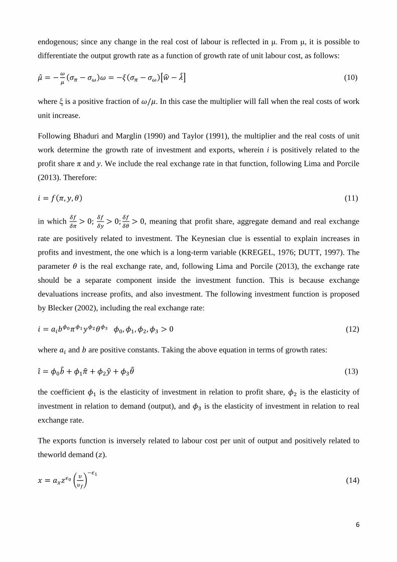
endogenous; since any change in the real cost of labour is reflected in μ. From μ, it is possible to

differentiate the output growth rate as a function of growth rate of unit labour cost, as follows:

�̂� = −𝜔

𝜇(𝜎𝜋 − 𝜎𝜔)𝜔 = −𝜉(𝜎𝜋 − 𝜎𝜔)[�̂� − �̂�] (10)

where ξ is a positive fraction of 𝜔/𝜇. In this case the multiplier will fall when the real costs of work

unit increase.

Following Bhaduri and Marglin (1990) and Taylor (1991), the multiplier and the real costs of unit

work determine the growth rate of investment and exports, wherein i is positively related to the

profit share π and y. We include the real exchange rate in that function, following Lima and Porcile

(2013). Therefore:

𝑖 = 𝑓(𝜋, 𝑦, 𝜃) (11)

in which 𝛿𝑓

𝛿𝜋> 0;

𝛿𝑓

𝛿𝑦> 0;

𝛿𝑓

𝛿𝜃> 0, meaning that profit share, aggregate demand and real exchange

rate are positively related to investment. The Keynesian clue is essential to explain increases in

profits and investment, the one which is a long-term variable (KREGEL, 1976; DUTT, 1997). The

parameter 𝜃 is the real exchange rate, and, following Lima and Porcile (2013), the exchange rate

should be a separate component inside the investment function. This is because exchange

devaluations increase profits, and also investment. The following investment function is proposed

by Blecker (2002), including the real exchange rate:

𝑖 = 𝑎𝑖𝑏𝜙0𝜋𝜙1𝑦𝜙2𝜃𝜙3 𝜙0, 𝜙1, 𝜙2, 𝜙3 > 0 (12)

where 𝑎𝑖 and 𝑏 are positive constants. Taking the above equation in terms of growth rates:

𝑖̂ = 𝜙0�̂� + 𝜙1�̂� + 𝜙2�̂� + 𝜙3𝜃 (13)

the coefficient 𝜙1 is the elasticity of investment in relation to profit share, 𝜙2 is the elasticity of

investment in relation to demand (output), and 𝜙3 is the elasticity of investment in relation to real

exchange rate.

The exports function is inversely related to labour cost per unit of output and positively related to

theworld demand (𝑧).

𝑥 = 𝑎𝑥𝑧𝜖0 (𝜐

𝜐𝑓)

−𝜖1

(14)

7

where 𝑎𝑥 is a positive constant, 𝜐𝑓 the real cost of work associated with exports, 𝜖0 the elasticity of

exports based on world demand and 𝜖1 is the elasticity of exports in relation to labour cost per unit

of output. Assuming that 𝜐𝑓 = 1 and 𝜖0 = 1; and linearizing equation (14) it is obtained the

following equation:

�̂� = �̂� − 𝜖1�̂� (15)

The exports grow with an increasing foreign demand and with decreasing unit labour costs.

Substituting equations, (4), (10), (13) and (15) into (9), it is obtained the follows:

�̂� =[𝜓𝑖𝜙0�̂�+𝜓𝑥�̂�+𝜓𝑖𝜙0�̂�]

[1−𝜓𝑖𝜙2]+

[𝜉(𝜎𝜋−𝜎𝜔)−𝜓𝑥𝜖1−𝜓𝑖𝜙1𝛼]

[1−𝜓𝑖𝜙2][�̂� − �̂�] (16)

Some results regarding the grow of the output:

1) In order to the autonomous components being meaningful, it is required that [1 − 𝜓𝑖𝜙2] >

0, since (0 < 𝜓𝑖 < 1), elasticity should fall with: 0 ≤ 𝜙2 < (1/𝜓𝑖);

2) In relation to growth rate of labour cost per unit of output [�̂� = (�̂� − �̂�)], the impact of

increased cost is ambiguous. If the growth of the real wage exceeds productivity growth

(�̂� > �̂�), which means (�̂� > 0), there will be two effects on output growth. On the one hand,

will reduce export and investment growth, and therefore the output. On the other hand, it

will increase the Keynesian multiplier, which means it will reduce the marginal propensity

to save, to distribute income from profits to wages.

3) Devaluation of the real exchange rate in a profit-led demand regime may increase the rate of

demand growth and the opposite happens if the demand regime is wage-led. In this case, the

impact of real depreciation of the exchange rate is also ambiguous.

If (1 − 𝜓𝑖𝜙2)>0 and differentiating equation (17) with respected to �̂�, the demand regime is wage-

led, which is show by the follow equation:

𝑑�̂�

𝑑�̂�= (𝜎𝜋 − 𝜎𝜔) > (

𝑖

𝜋𝑦) 𝜙1 + (

𝑥

𝜈𝑦) 𝜖1 (17)

If elasticity of the investment , based on profit share, and export cost elasticity are relatively smaller

than propensity to save (supposing that saving propensity by capitalists is greater than save

propensity by workers) then the demand regime is wage-led. In this scenario increases in wage

share will increase aggregate demand.

8

Conversely, if the export demand and the investment demand elasticities are higher than propensity

to save, the demand regime will be profit-led. This means that an increase in real wages will reduce

economic growth.

The interaction between productivity and demand regime, in a profit led economy, is represented

the following expression:

𝑑�̂�

𝑑�̂�> 0 if (𝜎𝜋 − 𝜎𝜔) < (

𝑖

𝜋𝑦) 𝜙1 + (

𝑥

𝜈𝑦) 𝜖1 (18)

If the derivative is taken in equation (17) relation to �̂�, the opposite result occurs (in comparison to

𝑑�̂� 𝑑�̂�⁄ ).

Under the wage-led regime, we have

𝑑�̂�

𝑑�̂�< 0 if (𝜎𝜋 − 𝜎𝜔) > (

𝑖

𝜋𝑦) 𝜙1 + (

𝑥

𝜈𝑦) 𝜖1 (19)

the negative impact on output growth of income redistribution implies that the growth rate of

productivity is greater than the effects of an increase in investments (via profit share) and exports

(via costs).

The derivative of equation (16) taken in relation to �̂� shows the demand led growth model:

𝑑�̂�

𝑑�̂�= 𝐶 =

[𝜉(𝜎𝜋−𝜎𝜔)−𝜓𝑥𝜖1−𝜓𝑖𝜙1𝛼]

[1−𝜓𝑖𝜙2] (20)

which has the equivalent interpretation as equation (17).

4. Results

This section brings tests for interaction among aggregate demand, real exchange rate, productivity

and real wages for the Brazilian economy, between 1960 and 2011 using the model developed

above. In order to calculate the demand regime, it will be estimate the follow equation:

Saving equation

𝜎 =𝑠

𝑦= 𝜎𝜋 + (𝜎𝜔 − 𝜎𝜋)𝜔 (6)

Investment equation

𝑖̂ = 𝜙0�̂� + 𝜙1�̂� + 𝜙2�̂� + 𝜙3𝜃 (13)

And export equation

9

�̂� = �̂� − 𝜖1�̂� (15)

The Gross Saving data was found on IPEADATA database, from 1960 to 2011. The Gross Saving

was deflated by Brazilian Index Consumer Prices (IPCA). The Gross Domestic Product (GDP) from

1960 to 2011 was also collected on IPEADATA database in real terms. The wage share data from

1960 to 2008 was used the same data presented by Marquetti e Porsse (2014) and from 2009 to

2011 the data for this variable can be found on National Account System (SCN) from Brazilian

Institute of Geography and Statistic (IBGE).

The data for Gross Fixed Capital Formation (investment) from 1960 to 2008 was obtained on

Marquetti e Porsse (2014). From 2009 to 2011 in IPEADATA database. The profit share is (𝜋 =

1 − 𝜔). In this case it is used the data for wage share, which was already explained the source. GDP

was also already explained the source. The real exchange rate was calculated in the usual manner:

𝜃 =𝑃∗

𝑃𝐸, where 𝑃∗ is U.S. producer prices base 100 in 2005, the source was IMF ; P is Brazil

consumer prices base 100 in 2005, the source was IPEADA; E is the end-of-period nominal

BRL/USD market exchange rate (buy); and 𝜃 is the real exchange rate,

The data for Brazilian export and World Income can be found on World Development Indicators

(WDI), World Bank, from 1960 to 2011. To calculated equation (2), or (𝑣 = �̂� − �̂�) is necessary

the data for real wage in growth rate and productivity in growth rate. From 1960 to 2008 the data

can be found in Marquetti e Porsse (2014) and from 2009 to 2011 the data for this variable can be

found on National Account System (SCN) from Brazilian Institute of Geography and Statistic

(IBGE).

10

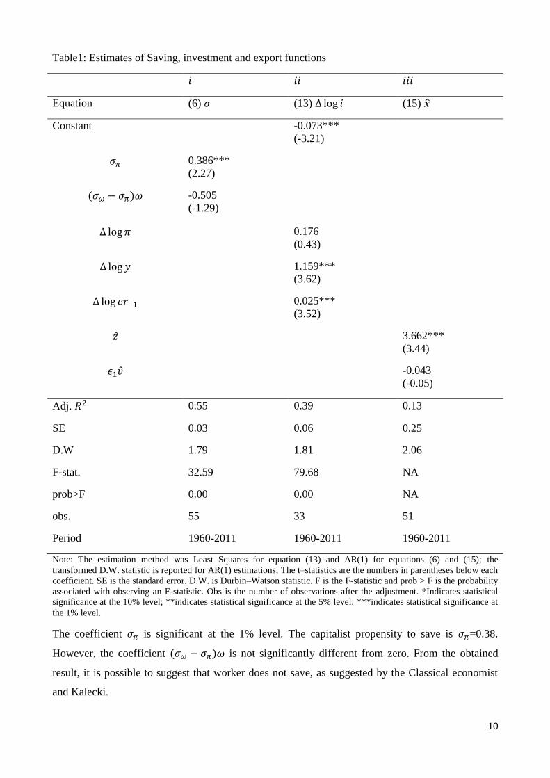
Table1: Estimates of Saving, investment and export functions

𝑖 𝑖𝑖 𝑖𝑖𝑖

Equation (6) 𝜎 (13) ∆ log 𝑖 (15) �̂�

Constant -0.073***

(-3.21)

𝜎𝜋 0.386***

(2.27)

(𝜎𝜔 − 𝜎𝜋)𝜔

-0.505

(-1.29)

∆ log 𝜋 0.176

(0.43)

∆ log 𝑦 1.159***

(3.62)

∆ log 𝑒𝑟−1 0.025***

(3.52)

�̂� 3.662***

(3.44)

𝜖1�̂� -0.043

(-0.05)

Adj. 𝑅2 0.55 0.39 0.13

SE 0.03 0.06 0.25

D.W 1.79 1.81 2.06

F-stat. 32.59 79.68 NA

prob>F 0.00 0.00 NA

obs. 55 33 51

Period 1960-2011 1960-2011 1960-2011

Note: The estimation method was Least Squares for equation (13) and AR(1) for equations (6) and (15); the

transformed D.W. statistic is reported for AR(1) estimations, The t–statistics are the numbers in parentheses below each

coefficient. SE is the standard error. D.W. is Durbin–Watson statistic. F is the F-statistic and prob > F is the probability

associated with observing an F-statistic. Obs is the number of observations after the adjustment. *Indicates statistical

significance at the 10% level; **indicates statistical significance at the 5% level; ***indicates statistical significance at

the 1% level.

The coefficient 𝜎𝜋 is significant at the 1% level. The capitalist propensity to save is 𝜎𝜋=0.38.

However, the coefficient (𝜎𝜔 − 𝜎𝜋)𝜔 is not significantly different from zero. From the obtained

result, it is possible to suggest that worker does not save, as suggested by the Classical economist

and Kalecki.

11

In relation to the investment equation (13), the coefficient related with the profit share is 0.176,

however, the mentioned coefficient is not statically different from zero, which means that

increasing in profit share does not raise investment, considering the Brazilian case. This coefficient

value considering the cases of France, Germany, Italy, UK and US, is on average (0.28) (STORM

& NAASTEPAD, 2007). However, the estimated coefficient in this exercise is not statistically

significant. On the other hand, the coefficients for demand is (1.159) and real exchange rate (0.025)

are both positive and statistically different from zero.

The result for the export equation (15) shows that the coefficient related with the real unit labour

cost has the expected sign (negative), however, this coefficient is not significantly different from

zero. Nevertheless the coefficient of world trade (�̂�) has the expected signal and it is significantly

different from zero. Therefore, this result rejects the possibility that reducing real wage would

increase the export growth rate.

To evaluate whether the demand regime is profit or wage led, equation (20A) is calculated. The

result is given below:

𝑑�̂�

𝑑�̂�= 𝐶 =

[𝜉(𝜎𝜋−𝜎𝜔)−𝜓𝑥𝜖1−𝜓𝑖𝜙1𝛼]

[1−𝜓𝑖𝜙2] = 0,176 (20)

Based on this result, the Brazilian economy is wage-led for the entire period (1960-2011).

5. Productivity

The model presented below builds on Naastepad (2006), Naastepad and Storm (2007) and Storm

and Naastepad (2012) by introducing a link between the exchange rate devaluation and productivity

in wage-led regime. On the other hand, even if the demand regime is profit-led, the exchange rate

devaluation can have a negative impact on productivity, hence on the economic growth. Besides,

the model includes a modified investment function presented in Storm and Naastepad (2012) by

imposing its dependence to the demand growth rate, the profit share and the real exchange rate,

following Missio and Jayme Jr. (2013).

According to Storm and Naastepad (2012), productivity is endogenous, depending demand and real

wage growth. The demand regime can be wage-led or profit-led. In both cases, an increase in real

wages can affect productivity positively through increasing spending on R&D, investment and

capital intensity in production. Silveira and Lima (2014) show that when wages increase, in a

heterogeneous firm environment, labour productivity also increases. This enhances the Storm and

Naastepad (2012) argument.

12

A simple equation of endogenous productivity growth can be expressed as follows:

�̂� = 𝛽0 + 𝛽1�̂� + 𝛽2�̂� + 𝛽3𝜃; 0 < 𝛽1 < 1; 𝛽2, > 0; 𝛽3 ≶ 0 (21)

Where �̂� is the growth rate of labour productivity, �̂� the growth rate of real output, �̂� the growth

rate of the real wage and 𝜃 the real exchange rate. 𝛽1 is the Kaldor-Verdoorn coefficient, i.e. the

growth in productivity is caused by increasing aggregate demand and output. The relation between

increasing productivity and demand growth can be expressed through the following channels: i)

improvements in the division of labour; ii) learning-by-doing; iii) increasing investment, as new

equipment and new methods can both enhance productivity (STORM and NAASTEPAD, 2012).

The coefficient 𝛽2 reflects a positive relationship between real wages growth and productivity

growth. The argument for this relationship refers to the Karl Marx’s idea of increasing real wages

leading to improvement in technical progress and innovation. Moreover, increasing in real wages

can also eliminate inefficient firms, favouring structural changes and raising the proportion of

skilled workers in the economy.

Regarding the coefficient 𝛽3, it reflects the indirect impact of the real exchange rate on productivity.

On one hand, the exchange rate can have negative indirect effects on productivity in the event of

devaluation. In this case, real wages will be reduced, thus it will decrease aggregate demand,

causing a reduction in industrial production and output, only if the demand regime is wage led.

Finally, it negatively impacts productivity.

Krugman and Taylor (1978) present three reasons why real exchange rate devaluation leads to

contractionary effects on aggregate demand. First, the depreciation of a currency raises exports and

imports prices. If trade is balanced, the terms of trade do not change, and an increase in import

prices is higher than exports, the net result will be a reduction of the country's income. Second, the

depreciation of the real exchange rate redistributes income from wages to profits. This happens for

two reasons: i) the monetary wages in the short term is rigid, then the depreciation of the exchange

rate reduces the real wage; ii) exports increase the income of exporters. Third, if the government

budget is unbalanced, it will have a compatible effect with impact on the income of the trade deficit.

If taxes are progressive, it will have a distribution on income from wages to profits, and greater

share on the economy of the collection tax, due to the devaluation. The devaluation transfers

income from the private sector to the public sector, since, assuming ad valorem taxes, depreciation

increases the price of imports, causing a positive impact on the collection of public sector.

Still, the coefficient 𝛽3 can be positive, as Missio and Jayme Jr. (2013) highlighted. They argue that

a higher real exchange rate (devaluation)level, it will increase the profit share, which affect the

13

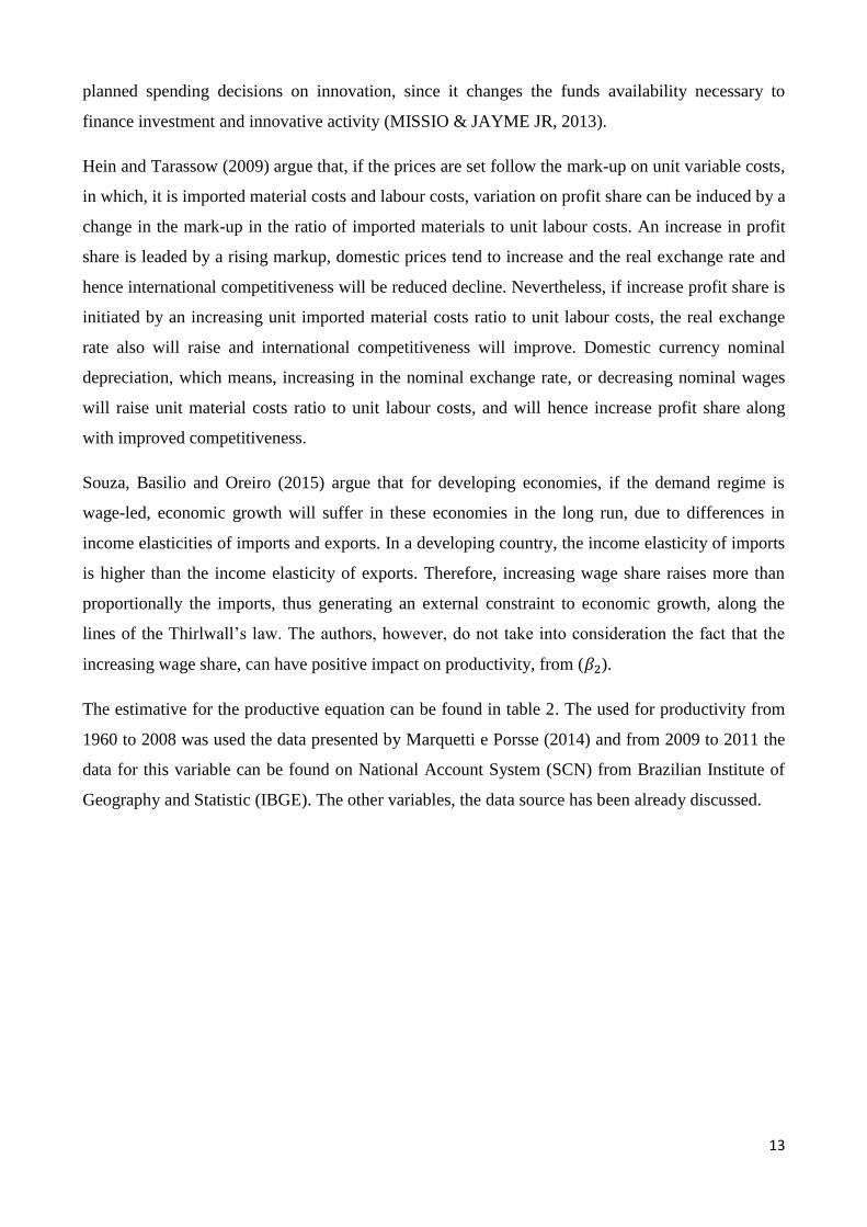
planned spending decisions on innovation, since it changes the funds availability necessary to

finance investment and innovative activity (MISSIO & JAYME JR, 2013).

Hein and Tarassow (2009) argue that, if the prices are set follow the mark-up on unit variable costs,

in which, it is imported material costs and labour costs, variation on profit share can be induced by a

change in the mark-up in the ratio of imported materials to unit labour costs. An increase in profit

share is leaded by a rising markup, domestic prices tend to increase and the real exchange rate and

hence international competitiveness will be reduced decline. Nevertheless, if increase profit share is

initiated by an increasing unit imported material costs ratio to unit labour costs, the real exchange

rate also will raise and international competitiveness will improve. Domestic currency nominal

depreciation, which means, increasing in the nominal exchange rate, or decreasing nominal wages

will raise unit material costs ratio to unit labour costs, and will hence increase profit share along

with improved competitiveness.

Souza, Basilio and Oreiro (2015) argue that for developing economies, if the demand regime is

wage-led, economic growth will suffer in these economies in the long run, due to differences in

income elasticities of imports and exports. In a developing country, the income elasticity of imports

is higher than the income elasticity of exports. Therefore, increasing wage share raises more than

proportionally the imports, thus generating an external constraint to economic growth, along the

lines of the Thirlwall’s law. The authors, however, do not take into consideration the fact that the

increasing wage share, can have positive impact on productivity, from (𝛽2).

The estimative for the productive equation can be found in table 2. The used for productivity from

1960 to 2008 was used the data presented by Marquetti e Porsse (2014) and from 2009 to 2011 the

data for this variable can be found on National Account System (SCN) from Brazilian Institute of

Geography and Statistic (IBGE). The other variables, the data source has been already discussed.

14

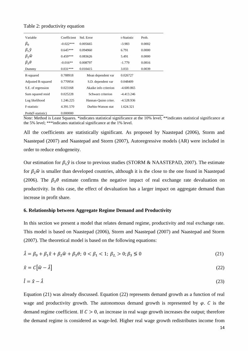
Table 2: productivity equation

Variable Coefficient Std. Error t-Statistic Prob.

𝛽0 -0.022*** 0.005665 -3.983 0.0002

𝛽1�̂� 0.645*** 0.094960 6.791 0.0000

𝛽2�̂� 0.459*** 0.083626 5.491 0.0000

𝛽3𝜃 -0.016** 0.008797 -1.779 0.0816

Dummy 0.031*** 0.010415 3.033 0.0039

R-squared 0.788918 Mean dependent var 0.026727

Adjusted R-squared 0.770954 S.D. dependent var 0.048409

S.E. of regression 0.023168 Akaike info criterion -4.600.865

Sum squared resid 0.025228 Schwarz criterion -4.413.246

Log likelihood 1.246.225 Hannan-Quinn criter. -4.528.936

F-statistic 4.391.570 Durbin-Watson stat 1.624.321

Prob(F-statistic) 0.000000

Note: Method is Least Squares. *indicates statistical significance at the 10% level; **indicates statistical significance at

the 5% level; ***indicates statistical significance at the 1% level.

All the coefficients are statistically significant. As proposed by Naastepad (2006), Storm and

Naastepad (2007) and Naastepad and Storm (2007), Autoregressive models (AR) were included in

order to reduce endogeneity.

Our estimation for 𝛽1�̂� is close to previous studies (STORM & NAASTEPAD, 2007). The estimate

for 𝛽2�̂� is smaller than developed countries, although it is the close to the one found in Naastepad

(2006). The 𝛽3𝜃 estimate confirms the negative impact of real exchange rate devaluation on

productivity. In this case, the effect of devaluation has a larger impact on aggregate demand than

increase in profit share.

6. Relationship between Aggregate Regime Demand and Productivity

In this section we present a model that relates demand regime, productivity and real exchange rate.

This model is based on Naastepad (2006), Storm and Naastepad (2007) and Naastepad and Storm

(2007). The theoretical model is based on the following equations:

�̂� = 𝛽0 + 𝛽1�̂� + 𝛽2�̂� + 𝛽3𝜃; 0 < 𝛽1 < 1; 𝛽2, > 0; 𝛽3 ≶ 0 (21)

�̂� = 𝐶[�̂� − �̂�] (22)

𝑙 = �̂� − �̂� (23)

Equation (21) was already discussed. Equation (22) represents demand growth as a function of real

wage and productivity growth. The autonomous demand growth is represented by 𝜑. 𝐶 is the

demand regime coefficient. If 𝐶 > 0, an increase in real wage growth increases the output; therefore

the demand regime is considered as wage-led. Higher real wage growth redistributes income from

15

profits towards wages and therefore, consumption growth is greater than the growth of investment

and exports. If 𝐶 < 0, an increase in real wage growth influences negatively the output growth, and

hence the demand regime is profit-led. Equation (23) expresses employment growth (𝑙) as a

difference between demand and productivity growth.

Using equation (21), employment growth can be expressed as a function of output growth:

𝑙 = (1 − 𝛽1)�̂� − 𝛽0 − 𝛽2�̂� − 𝛽3𝜃 (24)

Merging equations (21), (22) and (24), and solving for output, labour productivity and employment

growth, we get:

�̂� =𝜑−𝛽0𝐶

1+𝛽1𝐶+

(1−𝛽2)𝐶

1+𝛽1𝐶�̂� + [−

𝛽3𝐶

1+𝛽1𝐶 ]𝜃 = �̅� + �̅��̂� + 𝛿̅𝜃 (25)

�̂� = 𝛽0 + 𝛽1�̅� + [𝛽2 + 𝛽1�̅�]�̂� + (𝛽3 − 𝛽1𝛿̅)�̂� (26)

𝑙 = −𝛽0 + (1 − 𝛽1)�̅� + [(1 − 𝛽1)�̅� − 𝛽2]�̂� + [(1 − 𝛽1)𝛿̅ − 𝛽3]𝜃 (27)

Whereas: �̅� =𝜑−𝛽0𝐶

1+𝛽1𝐶, �̅� =

(1−𝛽2)𝐶

1+𝛽1𝐶 e 𝛿̅ = −

𝛽3𝐶

1+𝛽1𝐶.

6.1 The relationship between regime demand and real wage

Equations (25), (26) and (27) show how output growth, productivity and employment are affected

by changes in the real wage, in particular a reduction in real wage.

From equation (25), it is obtained:

𝑑�̂�

𝑑�̂�= �̅� =

(1−𝛽2)𝐶

1+𝛽1𝐶 (28)

Using the estimations from table 1 and the result of demand regime (𝐶 =0,176), which was obtained

from the equation (20), it is possible to calculate equation (28), in the following way:

𝑑�̂�

𝑑�̂�= �̅� =

(1−𝛽2)𝐶

1+𝛽1𝐶=

(1−0,459)0,176

1+0,645(0,176)= 0,085 (28’)

The total impact of an one-percentage-point decline in real wage growth on output growth is -0,085

percentage points. This one-percentage-point reduction in real wage growth decreases the profit

share by 0,176 percentage-points. The Kaldor-Verdoorn Effect is important to increase profit share

given that a raise in output growth has a significant impact on productivity growth (𝛽1). However,

reduction in real wage growth has a negative impact on productivity growth (𝛽2), which makes the

16

economy less wage-led, even though for the Brazilian economy, the (𝛽2) coefficient is smaller

compared to (𝛽1).

6.2 The relationship between regime demand and real exchange rate

Taking the derivative of equation (24) with respect to real exchange rate, we obtain:

𝑑�̂�

𝑑�̂�= 𝛿̅ = [−

𝛽3𝐶

1+𝛽1𝐶 ] (29)

The parameter 𝛽3 represents the relation between real exchange rate and productivity. Therefore,

we can have the following relations:

i) if 𝛽3 < 0 and 𝐶 > 0, the overall result is positive, which strengthens the wage led

feature of the demand regime. A decline in real wage growth has a negative impact on

output growth;

ii) if 𝛽3 < 0 and 𝐶 < 0, depreciation of the exchange rate reduces productivity, the overall

sign of the derivative will be negative, reinforcing the wage led demand regime;

iii) if 𝛽3 > 0 and 𝐶 > 0, exchange rate devaluations will reduce the demand;

iv) if 𝛽3 > 0 and 𝐶 < 0, the overall sign of the derivative will be positive, which means that

exchange rate devaluations will increase demand, reinforcing the profit-led demand

regime.

𝑑�̂�

𝑑�̂�= 𝛿̅ = −

𝛽3𝐶

1+𝛽1𝐶= − 0,00252 (29’)

The overall sign is negative, which means that exchange rate devaluations will decrease aggregate

demand, reinforcing the wage-led demand regime. Although the overall result is small, it suggest

that the real exchange rate devaluation can have a negative impact on productivity.

3.4.3 The relationship between demand regime and productivity

The total effect on productivity growth of a decline in real wage growth can be observed using

equations (1) and (27):

𝑑�̂�

𝑑�̂�= 𝛽2 + 𝛽1

𝑑�̂�

𝑑�̂�= 𝛽2 +

𝛽1(1−𝛽2)𝐶

1+𝛽1𝐶=

𝛽2+𝛽1𝐶

1+𝛽1𝐶 (30)

There are two effects related to the reduction of real wage growth on productivity. The direct effect

is through the 𝛽2∆�̂�, meaning that permanent reductions in real wages decline incentives to firms

invest in more efficient production techniques and therefore reducing the technical progress. The

indirect effect is through the Kaldor-Verdoorn multiplier 𝛽1. If the demand regime is wage-led the

17

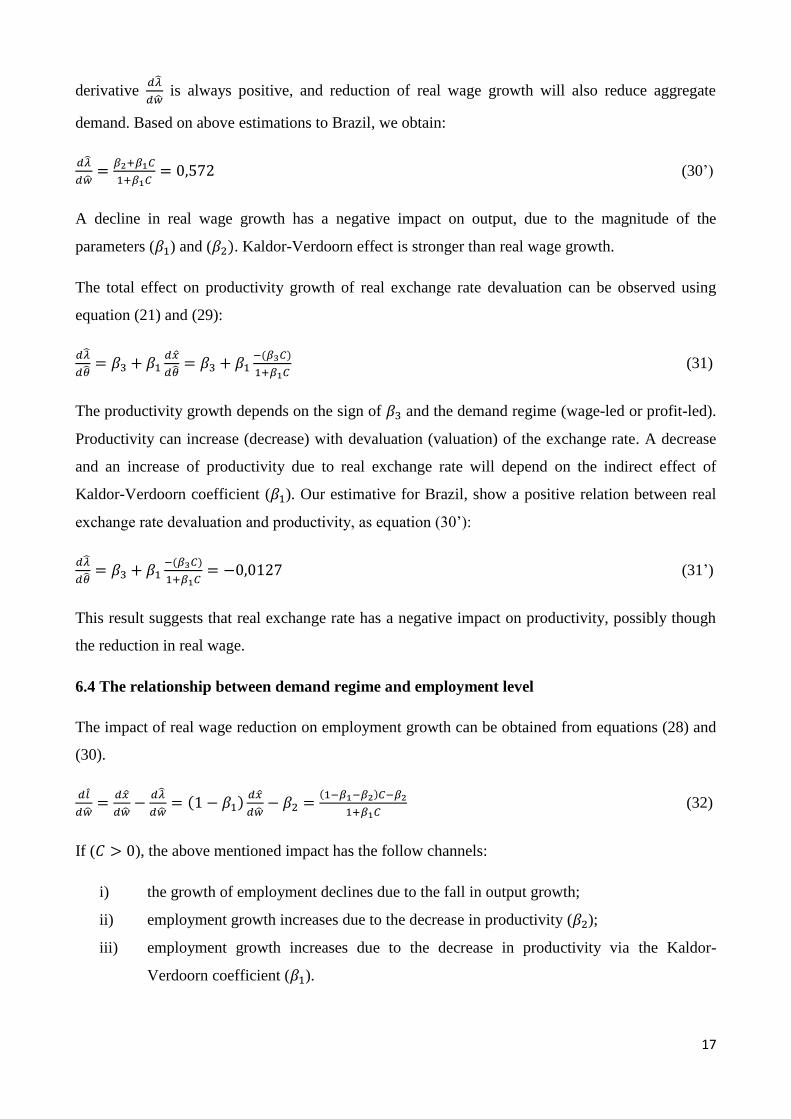
derivative 𝑑�̂�

𝑑�̂� is always positive, and reduction of real wage growth will also reduce aggregate

demand. Based on above estimations to Brazil, we obtain:

𝑑�̂�

𝑑�̂�=

𝛽2+𝛽1𝐶

1+𝛽1𝐶= 0,572 (30’)

A decline in real wage growth has a negative impact on output, due to the magnitude of the

parameters (𝛽1) and (𝛽2). Kaldor-Verdoorn effect is stronger than real wage growth.

The total effect on productivity growth of real exchange rate devaluation can be observed using

equation (21) and (29):

𝑑�̂�

𝑑�̂�= 𝛽3 + 𝛽1

𝑑�̂�

𝑑�̂�= 𝛽3 + 𝛽1

−(𝛽3𝐶)

1+𝛽1𝐶 (31)

The productivity growth depends on the sign of 𝛽3 and the demand regime (wage-led or profit-led).

Productivity can increase (decrease) with devaluation (valuation) of the exchange rate. A decrease

and an increase of productivity due to real exchange rate will depend on the indirect effect of

Kaldor-Verdoorn coefficient (𝛽1). Our estimative for Brazil, show a positive relation between real

exchange rate devaluation and productivity, as equation (30’):

𝑑�̂�

𝑑�̂�= 𝛽3 + 𝛽1

−(𝛽3𝐶)

1+𝛽1𝐶= −0,0127 (31’)

This result suggests that real exchange rate has a negative impact on productivity, possibly though

the reduction in real wage.

6.4 The relationship between demand regime and employment level

The impact of real wage reduction on employment growth can be obtained from equations (28) and

(30).

𝑑𝑙

𝑑�̂�=

𝑑�̂�

𝑑�̂�−

𝑑�̂�

𝑑�̂�= (1 − 𝛽1)

𝑑�̂�

𝑑�̂�− 𝛽2 =

(1−𝛽1−𝛽2)𝐶−𝛽2

1+𝛽1𝐶 (32)

If (𝐶 > 0), the above mentioned impact has the follow channels:

i) the growth of employment declines due to the fall in output growth;

ii) employment growth increases due to the decrease in productivity (𝛽2);

iii) employment growth increases due to the decrease in productivity via the Kaldor-

Verdoorn coefficient (𝛽1).

18

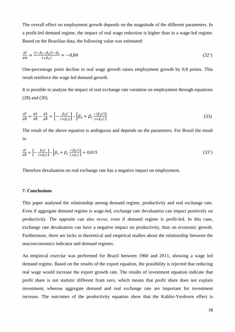
The overall effect on employment growth depends on the magnitude of the different parameters. In

a profit-led demand regime, the impact of real wage reduction is higher than in a wage-led regime.

Based on the Brazilian data, the following value was estimated:

𝑑𝑙

𝑑�̂�=

(1−𝛽1−𝛽2)𝐶−𝛽2

1+𝛽1𝐶= −0,84 (32’)

One-percentage point decline in real wage growth raises employment growth by 0,8 points. This

result reinforce the wage led demand growth.

It is possible to analyse the impact of real exchange rate variation on employment through equations

(28) and (30).

𝑑𝑙

𝑑�̂�=

𝑑�̂�

𝑑�̂�−

𝑑�̂�

𝑑�̂�= [−

𝛽3𝐶

1+𝛽1𝐶] – [𝛽3 + 𝛽1

−(𝛽3𝐶)

1+𝛽1𝐶] (33)

The result of the above equation is ambiguous and depends on the parameters. For Brazil the result

is:

𝑑𝑙

𝑑�̂�= [−

𝛽3𝐶

1+𝛽1𝐶] – [𝛽3 + 𝛽1

−(𝛽3𝐶)

1+𝛽1𝐶] = 0,015 (33’)

Therefore devaluation on real exchange rate has a negative impact on employment.

7. Conclusions

This paper analysed the relationship among demand regime, productivity and real exchange rate.

Even if aggregate demand regime is wage-led, exchange rate devaluation can impact positively on

productivity. The opposite can also occur, even if demand regime is profit-led. In this case,

exchange rate devaluation can have a negative impact on productivity, thus on economic growth.

Furthermore, there are lacks in theoretical and empirical studies about the relationship between the

macroeconomics indicator and demand regimes.

An empirical exercise was performed for Brazil between 1960 and 2011, showing a wage led

demand regime. Based on the results of the export equation, the possibility is rejected that reducing

real wage would increase the export growth rate. The results of investment equation indicate that

profit share is not statistic different from zero, which means that profit share does not explain

investment, whereas aggregate demand and real exchange rate are important for investment

increase. The outcomes of the productivity equation show that the Kaldor-Verdoorn effect is

19

considerable compared to real wage growth. The impact of real exchange rate on productivity

growth is negative but small; which might be due to the prolonged transmission mechanism.

Furthermore, a decline in real wage growth has a negative impact on output growth. A reduction in

real wage growth has a negative impact on productivity growth, which makes the economy wage-

led. Therefore, the interaction between demand regime and real exchange rate shows that

devaluation will have an ambiguous impact on the economy. On one hand, real exchange rate

devaluation has a positive relationship with investment. On the other hand, real exchange rate has a

negative impact on productivity. From the results found in this research, the Brazilian economy

operates in a wage led demand regime. In this scenario, real wage restraint is ineffective in reducing

unemployment; therefore a devaluation on real exchange rate has a negative impact on employment.

8. REFERENCES

AMADEO, Edward, J. Notes on growth, distribution and capacity utilization. Texto para discussão

no 116. Departamento de Economia, PUC-RJ, 1986.

BERTELLA, M. A. Modelos de Crescimento Kaleckianos: Uma Apreciação. Revista de

EconomiaPolítica, v. 27, p. 209-220, 2007.

BHADURI, A.; MARGLIN, S. (1990) Unemployment and the real wage: the economic basis for

contesting political ideologies, Cambridge Journal of Economics, 14, p. 375-393.

DOMAR, Evsey (1946). "Capital Expansion, Rate of Growth, and Employment". Econometrica 14

(2): 137–147, 1946.

DUTT, A.K. Stagnation, income distribution and monopoly power.Cambridge Journal of

Economics, 8, pp. 25-40, 1984.

DUTT, A. K. Growth, Distribution, and Uneven Development, Cambridge University Press, 1990.

FELIPE, J.; LAVIÑA, E.; FAN, E.(2008). The Diverging Patterns of Profitability, Investment and

Growth of China and India During 1980–2003. World Development, v. 36, n. 5, p. 741-

774.

FERRETTI, F. (2008). Patterns of technical change: a geometrical analysis using the wage-profit

rate schedule. International Review of Applied Economics, v. 22, n. 5, p. 565-583.

FOLEY, D., MICHL, T.R. (1999). Growth and Distribution.Harvard University Press, Cambridge,

MA.

20

FOLEY, D.; MARQUETTI, A. (1997).Economic growth from a classical prespective. In: Teixeira,

J (ed.). Money, growth, distribution and structural change: contemporaneos analysis.

Brasília: Editora da UnB.

FOLEY, D.; MARQUETTI, A, A. (1999).Productivity, Employment and Growth in European

Integration.Metroeconomica, v. 50, p. 277-300.

HARROD, R. International Economics. Cambridge: Cambridge University Press, 1933.

KALECKI, M. (2009) Theory of Economic Dynamics: An Essay on Cyclical and Long-Run

Changes in Capitalist Economy, Monthly Review Press.

KALDOR, N. (1966). Causes of the slow rate of economic growth of the United Kingdom: an

inaugural lecture. Cambridge: Cambridge University Press.

KRUGMAN, Paul; TAYLOR, Lance. Contractionary Effects of Devaluation. Journal

ofInternational Economics, 8(3): 445-456, 1978.

SETTERFIELD, M. (2003). Supply and Demand in the Theory of Long-run Growth: introduction

to a symposium on demand-led growth, Review of Political Economy, Volume 15,

Number 1, p, 23-32.

STORM, S., NAASTEPAD, C.W.M. (2012).Wage-led or profit-led supply: wages, productivity and

investment.Paper written for the projectNew perspectives on wages and economic growth:

the potentials ofwage-led growth.

VERDOORN, P.J. (1949). Fattoricheregolanolosviluppodellaproduttivita Del lavoro. L’industria.

No. 1, p. 3-10, 1949.

MARQUETTI, A. (2000). Estimativa do estoque de riqueza tangível no Brasil, 1950-1998. Nova

Economia, vol. 10, n. 2, p. 11-38.

MARQUETTI, A. (2002). Progresso técnico, distribuição e crescimento na economia brasileira:

1955-1998. Estudos Econômicos, v. 32, n. 1, p. 103-124.

MARQUETTI, A. e PORSSE, M. (2014) Padrões de Progresso Técnico na Economia Brasileira:

1952-2008. Revista da Cepal.

MISSIO, F. ; JAYME JR, F. G. . Restrição externa, nível da taxa real de câmbio e crescimento em

um modelo com progresso técnico endógeno. Economia e Sociedade (UNICAMP.

Impresso), v. 22, p. 367-407, 2013.

21

NAASTEPAD, C. W. M. Technology, demand and distribution: application to the Dutch

productivity growth slowdown. Cambridge Journal of Economics, no. 30, p. 403-34, 2006.

NAASTEPAD, C. W. M; STORM, Servaas. OECD demand regimes (1960-2000). Journal of Post-

Keynesian Economics, 29 (2), pp 211-246, 2007.

ONARAN,Ozlem, STOCKHAMMER,Engelbert. The Effect of Distribution on Accumulation,

Capacity Utilization and Employment: Testing the Wage-Led Hypothesis for

Turkey. Working Papers 0130, Economic Research Forum, revised, Oct 2001.

PALLEY, Thomas I. Inside Debt, Aggregate Demand, and the Cambridge Theory of

Distribution. Cambridge Journal of Economics, Oxford University Press, vol. 20(4), pages

465-74, July, 1996.

ROBINSON, J. The Accumulation of Capita.Macmillan, 1956.

_________.Essays in the Theory of Economic Growth.Macmillan, 1962.

ROWTHORN, R. Demand, Real Wages and Economic Growth.in Sawyer, M. C.(1988), Post-

Keynesian Economics, Edward Elgar, 1982.

ROMER, P. M. Increasing Returns and Long-Run Growth. Journal of Political Economy

Vol. 94, No. 5, pp. 1002-1037, 1986.

ROMER, P. M. Endogenous Technological Change. Journal of Political Economy. Vol. 98, No. 5,

Part 2: The Problem of Development: A Conference of the Institute for the Study of Free

Enterprise Systems, pp. S71-S102, 1990.

STOCKHAMMER, Engelbert. Robinsonian and Kaleckian Growth.An Update on Post-Keynesian

Growth Theories. Department of Economics Working Papers wuwp067, Vienna University

of Economics, Department of Economics, 1999.

TAYLOR, L. (1991). Lectures in Struturalism Macroeconomics, Cambridge, MA MIT Press.

TAVARES, Maria da C. A Retomada da hegemonia norte-americana. Revista de Economia

Política, v. 5, n. 2, p. 5-15, abr./jun. 1985.