DOUBLE STAR PM MACHINE SIMULATIONS - … · DOUBLE STAR PM MACHINE: ANALYSIS AND ... 1.3 Types of...

POLITECNICO DI MILANO

Scuola di Ingegneria Industriale e dell’Informazione

Corso di Laurea Magistrale in Ingegneria Elettrica

DOUBLE STAR PM MACHINE: ANALYSIS AND

SIMULATIONS

RELATORE: Prof. Stefania Maria CARMELI

CORRELATORE

Anno Accademico 2015-2016

TESI DI LAUREA DI:

Domenico CARDINALE

Matr. 817122

Ringrazio la mia famiglia per avermi

permesso di intraprendere questi studi

supportandomi lungo tutti questi anni, saluto

e ringrazio anche tutti i miei amici.

Un sentito ringraziamento alla Professoressa

Stefania Maria Carmeli per il suo

indispensabile aiuto nel compimento di

questa tesi e per la sua disponibilità e

pazienza

Contents

1 Introduction . . . . . . . . . . . . . . . . . . . . . . . . . . . . . . . . . . . . . . . . . . . . 1

1.1 Historical reasons . . . . . . . . . . . . . . . . . . . . . . . . . . . . . . . . . . . . . . . . . . . . . . . . . . . . . . . . . . . . . . . . . . . . . 1

1.2 About power converters . . . . . . . . . . . . . . . . . . . . . . . . . . . . . . . . . . . . . . . . . . . . . . . . . . . . . . . . . . . . . . 2

1.3 Types of multiphase machines . . . . . . . . . . . . . . . . . . . . . . . . . . . . . . . . . . . . . . . . . . . . . . . . . . . . . . . . 3

1.4 Stator windings . . . . . . . . . . . . . . . . . . . . . . . . . . . . . . . . . . . . . . . . . . . . . . . . . . . . . . . . . . . . . . . . . . . . . . . . 4

1.4.1 Machines with sinusoidal winding distribution . . . . . . . . . . . . . . . . . . . . . . . . . . . . . . . . . . . . . . . . 5

1.4.2 Concentrated winding machines. . . . . . . . . . . . . . . . . . . . . . . . . . . . . . . . . . . . . . . . . . . . . . . . . . . . 5

1.5 Sizing equations for multiphase machines. . . . . . . . . . . . . . . . . . . . . . . . . . . . . . . . . . . . . . . . . . . . . . 6

1.6 Advantages of multiphase machines. . . . . . . . . . . . . . . . . . . . . . . . . . . . . . . . . . . . . . . . . . . . . . . . . . . 9

1.6.1 Electric power segmentation . . . . . . . . . . . . . . . . . . . . . . . . . . . . . . . . . . . . . . . . . . . . . . . . . . . . . 9

1.6.2 Reliability and fault tolerance . . . . . . . . . . . . . . . . . . . . . . . . . . . . . . . . . . . . . . . . . . . . . . . . . . . . . 10

1.6.3 Performances . . . . . . . . . . . . . . . . . . . . . . . . . . . . . . . . . . . . . . . . . . . . . . . . . . . . . . . . . . . . . . . . . . . 11

2 Double star synchronous machine’s applications . . . . . . 13

2.1 Electric drive system of dual-winding fault-tolerant permanent-magnet motor

for aerospace applications. . . . . . . . . . . . . . . . . . . . . . . . . . . . . . . . . . . . . . . . . . . . . . . . . . . . . . . . .

13

2.1.1 Open-circuit and short-circuit condition. . . . . . . . . . . . . . . . . . . . . . . . . . . . . . . . . . . . . . . . 17

2.2 Split-phase machine for electric vehicles applications. . . . . . . . . . . . . . . . . . . . . . . . . . . . . 19

2.3 Ship applications: electric and hybrid electric propulsion. . . . . . . . . . . . . . . . . . . . . . . . . . 21

2.3.1 Cycloconverter systems. . . . . . . . . . . . . . . . . . . . . . . . . . . . . . . . . . . . . . . . . . . . . . . . . . . . 23

2.3.2 Synchronous converter systems. . . . . . . . . . . . . . . . . . . . . . . . . . . . . . . . . . . . . . . . . . . . . . 24

2.4 Locomotive traction system . . . . . . . . . . . . . . . . . . . . . . . . . . . . . . . . . . . . . . . . . . . . . . . . . . . 27

2.4.1 𝐵𝐵 26000 locomotive system. . . . . . . . . . . . . . . . . . . . . . . . . . . . . . . . . . . . . . . . . . . . . . . 27

3 Double star synchronous machine . . . . . . . . . . . . . . . . . . . 29

3.1: Description of the machine . . . . . . . . . . . . . . . . . . . . . . . . . . . . . . . . . . . . . . . . . . . . . . . . . . . 29

3.1.1 Rotor configurations. . . . . . . . . . . . . . . . . . . . . . . . . . . . . . . . . . . . . . . . . . . . . . . . . . . . . . 30

3.1.2 No load 𝐸𝑀𝐹. . . . . . . . . . . . . . . . . . . . . . . . . . . . . . . . . . . . . . . . . . . . . . . . . . . . . . . . . . . . 37

3.1.3 Hypotheses. . . . . . . . . . . . . . . . . . . . . . . . . . . . . . . . . . . . . . . . . . . . . . . . . . . . . . . . . . . . . 38

3.2: Phase variable model. . . . . . . . . . . . . . . . . . . . . . . . . . . . . . . . . . . . . . . . . . . . . . . . . . . . . . . . . 38

3.2.1 Model structure.. . . . . . . . . . . . . . . . . . . . . . . . . . . . . . . . . . . . . . . . . . . . . . . . . . . . . . . . . 38

3.2.2 Inductances. . . . . . . . . . . . . . . . . . . . . . . . . . . . . . . . . . . . . . . . . . . . . . . . . . . . . . . . . . . . . 39

3.2.3 Inductance waveforms. . . . . . . . . . . . . . . . . . . . . . . . . . . . . . . . . . . . . . . . . . . . . . . . . . . . . 39

3.2.4 Inductance matrix. . . . . . . . . . . . . . . . . . . . . . . . . . . . . . . . . . . . . . . . . . . . . . . . . . . . . . . . 40

3.2.5 Electromagnetic torque. . . . . . . . . . . . . . . . . . . . . . . . . . . . . . . . . . . . . . . . . . . . . . . . . . . . 41

3.3 Transformed variables model. . . . . . . . . . . . . . . . . . . . . . . . . . . . . . . . . . . . . . . . . . . . . . . . . . . 42

3.3.1 Introduction. . . . . . . . . . . . . . . . . . . . . . . . . . . . . . . . . . . . . . . . . . . . . . . . . . . . . . . . . . . . 42

3.3.2 Park transformation matrix. . . . . . . . . . . . . . . . . . . . . . . . . . . . . . . . . . . . . . . . . . . . . . . . . 42

3.3.3 transformed model. . . . . . . . . . . . . . . . . . . . . . . . . . . . . . . . . . . . . . . . . . . . . . . . . . . . . . . 45

3.2.5 Electromagnetic torque. . . . . . . . . . . . . . . . . . . . . . . . . . . . . . . . . . . . . . . . . . . . . . . . . . . . 46

3.3.5 Equivalent circuit. . . . . . . . . . . . . . . . . . . . . . . . . . . . . . . . . . . . . . . . . . . . . . . . . . . . . . . . . 47

4 Control strategies. . . . . . . . . . . . . . . . . . . . . . . . . . . . . . . . . . . 49

4.1 Wind turbines general characteristics. . . . . . . . . . . . . . . . . . . . . . . . . . . . . . . . . . . . . . . . . . . 49

4.1.1 Generalities. . . . . . . . . . . . . . . . . . . . . . . . . . . . . . . . . . . . . . . . . . . . . . . . . . . . . . . . . . . . . 49

4.1.2 Variable speed wind turbine’s regulation systems. . . . . . . . . . . . . . . . . . . . . . . . . . . . . . . . 52

4.1.3 Pitch regulation system. . . . . . . . . . . . . . . . . . . . . . . . . . . . . . . . . . . . . . . . . . . . . . . . . . . . 53

4.1.4 Synchronous generator system configuration. . . . . . . . . . . . . . . . . . . . . . . . . . . . . . . . . . . 54

4.2 Power converter control strategies .. . . . . . . . . . . . . . . . . . . . . . . . . . . . . . . . . . . . . . . . . . . . 55

4.2.1 Sinusoidal pulse width modulation. . . . . . . . . . . . . . . . . . . . . . . . . . . . . . . . . . . . . . . . . . . 55

4.2.2 Space vector modulation. . . . . . . . . . . . . . . . . . . . . . . . . . . . . . . . . . . . . . . . . . . . . . . . . . . 57

61

5 Simulations . . . . . . . . . . . . . . . . . . . . . . . . . . . . . . . . . . . . . . . . .

5.1 Machine data. . . . . . . . . . . . . . . . . . . . . . . . . . . . . . . . . . . . . . . . . . . . . . . . . . . . . . . . . . . . . . . . . 61

5.2 Machine model. . . . . . . . . . . . . . . . . . . . . . . . . . . . . . . . . . . . . . . . . . . . . . . . . . . . . . . . . . . . . . . 62

5.3 Torque expression. . . . . . . . . . . . . . . . . . . . . . . . . . . . . . . . . . . . . . . . . . . . . . . . . . . . . . . . . . . . . 64

5.4 PI regulator tuning. . . . . . . . . . . . . . . . . . . . . . . . . . . . . . . . . . . . . . . . . . . . . . . . . . . . . . . . . . . . 64

5.4.1 Current regulator.. . . . . . . . . . . . . . . . . . . . . . . . . . . . . . . . . . . . . . . . . . . . . . . . . . . . . . . . 64

5.4.2 Speed regulator design. . . . . . . . . . . . . . . . . . . . . . . . . . . . . . . . . . . . . . . . . . . . . . . . . . . . 66

5.5 Mechanical load equation. . . . . . . . . . . . . . . . . . . . . . . . . . . . . . . . . . . . . . . . . . . . . . . . . . . . . . 67

5.6 Park’s transformations. . . . . . . . . . . . . . . . . . . . . . . . . . . . . . . . . . . . . . . . . . . . . . . . . . . . . . . . . 68

5.7 Motor mode operation. . . . . . . . . . . . . . . . . . . . . . . . . . . . . . . . . . . . . . . . . . . . . . . . . . . . . . . . 69

5.7.1 System configuration. . . . . . . . . . . . . . . . . . . . . . . . . . . . . . . . . . . . . . . . . . . . . . . . . . . . . . 69

5.7.2 Simulation results. . . . . . . . . . . . . . . . . . . . . . . . . . . . . . . . . . . . . . . . . . . . . . . . . . . . . . . . 71

5.8 Generator mode operation (modulator as unity gain). . . . . . . . . . . . . . . . . . . . . . . . . . . . . 76

5.8.1 System configuration.. . . . . . . . . . . . . . . . . . . . . . . . . . . . . . . . . . . . . . . . . . . . . . . . . . . . . 76

5.8.2 Simulation results. . . . . . . . . . . . . . . . . . . . . . . . . . . . . . . . . . . . . . . . . . . . . . . . . . . . . . . . 77

5.9 Generator mode operation (complete model).. . . . . . . . . . . . . . . . . . . . . . . . . . . . . . . . . . . 81

5.9.1 System configuration . . . . . . . . . . . . . . . . . . . . . . . . . . . . . . . . . . . . . . . . . . . . . . . . . . . . . . 81

5.9.2 Description of the simulation. . . . . . . . . . . . . . . . . . . . . . . . . . . . . . . . . . . . . . . . . . . . . . . . 82

5.9.3 Six leg converter. . . . . . . . . . . . . . . . . . . . . . . . . . . . . . . . . . . . . . . . . . . . . . . . . . . . . . . . . 84

5.9.4 Simulation results . . . . . . . . . . . . . . . . . . . . . . . . . . . . . . . . . . . . . . . . . . . . . . . . . . . . . . . . 86

5.10 Generator mode operation with uncontrolled bridge . . . . . . . . . . . . . . . . . . . . . . . . . . . . 93

5.10.1 System configuration. . . . . . . . . . . . . . . . . . . . . . . . . . . . . . . . . . . . . . . . . . . . . . . . . . . . . 93

5.10.2 DC bus voltage control. . . . . . . . . . . . . . . . . . . . . . . . . . . . . . . . . . . . . . . . . . . . . . . . . . . . 93

5.10.3 Simulation. . . . . . . . . . . . . . . . . . . . . . . . . . . . . . . . . . . . . . . . . . . . . . . . . . . . . . . . . . . . . 94

5.10.4 Innovative control set up. . . . . . . . . . . . . . . . . . . . . . . . . . . . . . . . . . . . . . . . . . . . . . . . . . 96

Conclusions and further works

Bibliography

Acronyms and Symbols

𝑃𝑊𝑀: pulse width modulation

𝑉𝑆𝐼: voltage source inverter

𝐷𝑇𝐶: direct torque control

𝐷𝐶: direct current

𝐴𝐶: alternating current

𝑀𝑀𝐹: magneto motive force

𝐵𝐷𝐶𝑀: brushless DC machine

𝐼𝐺𝐵𝑇: insulated gate bipolar transistor

𝑃𝑀: permanent magnet

𝐷𝐹𝑃𝑀: doubly fed permanent magnet motor

𝐸𝑀𝐹: electromotive force

𝑆𝑉𝑃𝑊𝑀: space vector pulse width modulation

𝐹𝑂𝐶: field oriented control

𝑀𝑇𝑃𝐴: maximum torque per ampere method

𝑃𝑀𝑆𝑀: permanent magnet synchronous machine

𝐼𝑃𝑀: interior permanent magnets

𝑆𝑃𝑀: surface permanent magnets

𝐶𝑆𝐼: current source inverter

𝐷𝐹𝐼𝐺: doubly fed induction generator

𝑊𝑇: wind turbine

𝑇𝑆𝑅: tip speed ratio

𝑇𝐹: transfer function

𝑃𝐼: proportional integral regulator

𝑉 , : voltage and current, respectively

𝑛: number of phases of an electrical machine

𝛼: displacement between any two consecutive stator phases

𝑘, 𝑖: number of windings and number of sub phases

𝑁: number of three phase winding sets

N𝑠: number of series connected turns per phase

Φ𝑃: per pole flux

Φ𝑔: air gap flux

K𝑤: winding factor

𝑓: frequency of electrical quantities (𝐻𝑧)

𝐿: useful core length

𝐷: diameter of the air gap

𝑝: number of poles

𝑛𝑝: number of pole pairs

𝑛𝑟𝑝𝑚: rotor rotational speed 𝑟𝑝𝑚 of the electrical machine

N𝑡: number of series connected turns per coil

𝑞: number of slots per pole per phase

𝑏: number of parallel path per phase

𝜏𝑠: slot pitch

𝜎𝑠: current density

𝜆𝑠: electric loading

𝐶: output coefficient

𝑃, 𝑃𝑚: electrical (active) and mechanical power, respectively

𝐴𝑡 , 𝐴𝑠: turn and slot cross section area

𝐾𝑓: fill factor of a stator slot

𝑎𝑖 , 𝑏𝑖 , 𝑐𝑖: phases’ name in the 𝑖𝑡ℎ winding set

𝐼𝑠𝑐: short circuit current

𝐸0 , 𝐸𝐿2𝐿: no load 𝐸𝑀𝐹 phase and line to line value, respectively

𝜔𝑒 : electrical angular speed of the rotor (𝑒𝑙. 𝑟𝑎𝑑 𝑠⁄ )

𝑅𝑠 : stator resistance

𝐿𝑠 : stator inductance

𝐿𝑠𝜎: leakage inductance

𝐿𝑠𝑚: excitation inductance

𝑇𝑚𝑎𝑥: maximum torque

𝑇𝑒 : electromagnetic torque

𝑂1 𝑂2: neutral point of the first and second winding set respectively

𝑇𝑚: mechanical resistance torque

Φ𝑒 , Φ𝑎: excitation and armature flux, respectively

𝛾: angle between excitation and armature flux

𝐵 : magnetic induction

𝐻: magnetic field intensity

𝜇0: absolute permeability

𝐴𝑚 , ℎ𝑚 , 𝑉𝑚 , 𝑈𝑚: area, length, volume and magnetic voltage of the permanent magnet

𝐴𝑔 , ℎ𝑔 , 𝑉𝑔 , 𝑈𝑔: area, length, volume and magnetic voltage of the air gap

Ψ𝑃𝑀 : permanent magnets flux

𝐿, 𝑀: self and mutual inductance

𝜔𝑚 : mechanical angular speed of the rotor (𝑟𝑎𝑑 𝑠⁄ )

𝜃𝑒: electrical angle

𝜃𝑚: mechanical angle

𝛼 − 𝛽: stationary reference frame

𝑑 − 𝑞: reference frame synchronous with rotor position

𝑆: wind passage area in wind turbine

𝑣: wind speed

Ω𝑟 , n𝑟: angular speed of wind turbine’s blades (𝑟𝑎𝑑/𝑠 and 𝑟𝑝𝑚, respectively)

D𝑏 , 𝑟: diameter and radius of the blades of the wind turbine

𝜌: air density

𝑐𝑝: power coefficient

𝜆: tip speed ratio

𝛽: pitch angle

𝑚𝑎 , 𝑚𝑓: amplitude modulation ratio and frequency modulation ratio

𝑓ℎ, ℎ: frequency of harmonic component and harmonic order respectively

𝐽: inertia

𝐵𝑣: viscious friction coefficient

𝐾𝑝 , 𝐾𝑖 : PI regulator parameters

𝑔1 , 𝑔2: gate control signals

𝑉𝐷𝐶: 𝐷𝐶 bus voltage

𝐼𝐷𝐶: 𝐷𝐶 side current

𝜂: efficiency

Figures list

Figure 1.1: possible configuration with multiphase machines

Figure 1.2: types of stator slots (open slots)

Figure 1.3: schematic phase arrangment of a split phase machine with 𝑁 three phase winding sets

Figure 1.4: four phases windings machine

Figure 1.5: (a) three phase configuration (b) multi-star configuration (c) symmetrical polyphase

configuration

Figure 1.6: (a) multi-phase machine supplied by 𝑁 𝑛-phase inverters (b) example of 19 𝑀𝑊15-

phase induction motor with 𝑁 = 3 and 𝑛 = 5

Figure 2.1: redundant motor topology

Figure 2.2: cross section of the motor

Figure 2.3: control scheme for fault diagnosis

Figure 2.4: (a) open circuit fault (b) short circuit fault

Figure 2.5: traction/charge circuit in electric vehicle

Figure 2.6 equivalent circuit during charge operation

Figure 2.7: Principle scheme of the class 𝑇2 tanker

Figure 2.8: Queen Elizabeth ship principle scheme

Figure 2.9: block diagram a cycloconverter

Figure 2.10: three phase cycloconverter

Figure 2.11: double star synchronous machine drives by 12 pulse bridge

Figure 2.12: ship’s propulsion using synchro-converter

Figure 2.13: current waveforms using synchro-converter

Figure 2.14: step’s advancing currents

Figure 2.15: double star synchronous machine used in synchro-converter fed system

Figure 2.16: principle scheme of one of the two traction motor

Figure 2.17: input stage of 𝐵𝐵 26000 locomotive

Figure 3.1: windings arrangement in double star synchronous machine

Figure 3.2: flux density vs magnetizing field

Figure 3.4: (a) surface 𝑃𝑀 (b) interior 𝑃𝑀

Figure 3.5: maximum energy product

Figure 3.6: (a)surface permanent magnets (b) interior permanent magnets

Figure 3.7: inductance waveforms

Figure 3.8: graphical representation of the transformation

Figure 3.9: d-axis equivalent circuit Figure 3.10: q-axis equivalent circuit

Figure 4.1: (a) wind turbine blades and relative speeds (b) air flow

Figure 4.2: 𝑐𝑝vs 𝑇𝑆𝑅 at constant pitch angle

Figure 4.3: (a) Power coefficient as a function of 𝑇𝑆𝑅 for a given turbine (b) extracted power for

𝑐𝑝 = 𝑐𝑝𝑚𝑎𝑥

Figure 4.4: (a) wind turbine’s control system (b) generator rotational speed and consequent

generated power

Figure 4.5: scheme of the 𝑃𝑀𝑆𝐺 drive

Figure 4.6: possible configuration of 𝑃𝑀𝑆𝑀 drives: high, medium and low speed

Figure 4.7: (a) pulse width modulation (b) harmonic content

Figure 4.8: six leg converter structure

Figure 4.9: (a) possible converter states (b) graph of consecutive transitions (c) example of reference

vector

Figure 4.10: (a) six leg converter control strategy first case (b) six leg converter control strategy

second case

Figure 4.11: vector classification technique

Figure 5.1: machine model

Figure 5.2: disturbances

Figure 5.3 torque expression

Figure 5.4: procedure to find 𝐾𝑝 , 𝐾𝑖 gains

Figure 5.5: time domain response

Figure 5.6: frequency domain response

Figure 5.7: speed loop design scheme

Figure 5.8: transfer function and sensitivity function

Figure 5.9: mechanical load equation

Figure 5.10: Park’s transformation

Figure 5.11: complete simulated model

Figure 5.12: mechanical vs electromagnetic torque

Figure 5.13: reference vs actual speed

Figure 5.14: 𝑞1 current component

Figure 5.15: 𝑑1 current component



Figure 5.18: phase currents of the two winding sets

Figure 5.19: electrical power vs mechanical power

Figure 5.20: rotational speed imposed by the prime mover

Figure: 5.21: generator simulation without modulator

Figure 5.22: actual vs reference electromagnetic torque

Figure 5.23: 𝑖𝑞1 current component

Figure 5.24: 𝑖𝑑1 current component

Figure 5.25: (a) 𝑖𝑑2 current component (b) 𝑖𝑞2

current component

Figure 5.26: phase currents in generator mode operation


Figure 5.28: studied configuration system

Figure 5.29: single leg converter operation

Figure 5.29: complete system for motor mode operation

Figure 5.30: (a) rectifier mode operation (b) inverter mode operation both in unity power factor

operation


Figure 5.32: control system

Figure 5.33: gate signal generators

Figure 5.34: inverter and 𝐷𝐶 link model









Figure 5.43: actual phase voltages (first winding set)

Figure 5.44: first harmonic of 𝑣𝑎1

Figure 5.45: 𝐴𝐶 variables

Figure 5.46: 𝐷𝐶 side current

Figure 5.47: mechanical vs electrical power

Figure 5.48: (a) electrical circuit model (b) DC bus voltage regulation

Figure 5.49: (a) mechanical power (b) 𝐼𝑟𝑒𝑓 selection

Figure 5.50: regulated 𝐷𝐶 voltage Figure 5.51: electromagnetic torque (uncontrolled diode bridge)

Figure 5.52: 𝑖𝑑1 current component (uncontrolled bridge)

Figure 5.53: 𝑖𝑞1 current component (uncontrolled bridge)

Figure 5.54: mechanical and electrical powers (uncontrolled bridge)

Figure 5.55: (a) system configuration (b) 𝐷𝐶 bus regulation

Figure 5.56: corrective term control system

Tables

Table 1: Uses of additional degrees of freedom

Table 2: fault diagnosis methods

Table 3: main properties of hard magnetic materials

Table 4: value of inductance harmonics

Table 5: machine data

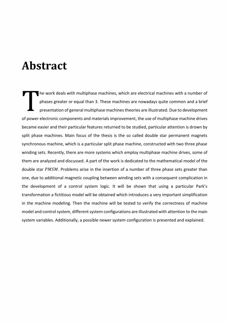
Abstract

he work deals with multiphase machines, which are electrical machines with a number of

phases greater or equal than 3. These machines are nowadays quite common and a brief

presentation of general multiphase machines theories are illustrated. Due to development

of power electronic components and materials improvement, the use of multiphase machine drives

became easier and their particular features returned to be studied, particular attention is drown by

split phase machines. Main focus of the thesis is the so called double star permanent magnets

synchronous machine, which is a particular split phase machine, constructed with two three phase

winding sets. Recently, there are more systems which employ multiphase machine drives, some of

them are analyzed and discussed. A part of the work is dedicated to the mathematical model of the

double star 𝑃𝑀𝑆𝑀. Problems arise in the insertion of a number of three phase sets greater than

one, due to additional magnetic coupling between winding sets with a consequent complication in

the development of a control system logic. It will be shown that using a particular Park’s

transformation a fictitious model will be obtained which introduces a very important simplification

in the machine modeling. Then the machine will be tested to verify the correctness of machine

model and control system, different system configurations are illustrated with attention to the main

system variables. Additionally, a possible newer system configuration is presented and explained.

T

Summary

Chapter 1 is a brief introduction of multiphase machines’ generalities. In particular, an

introduction about their sizing equation stator and rotor windings, advantages and disadvantages

arises by adding a number of machine phases greater or equal than three.

Chapter 2 illustrates some applicative cases in the use of the double star 𝑆𝑀. Its use is spread in

many application areas such as: more electric aircraft, ship applications, automobile and rail traction

drives.

Chapter 3 Shows the mathematical model of the double star 𝑃𝑀𝑆𝑀. Phase variables model is

transformed using a particular Park’s transformation and obtained results, such as: decoupling,

torque expression simplification, possible use of general three phase machine theory are presented

and discussed.

Chapter 4 Brief introduction to wind turbine systems: maximum extractable wind power,

possible system configuration, with particular attention to 𝑃𝑀𝑆𝑀 system configuration. Some

power converter’s control strategies, such as: 𝑃𝑊𝑀 and space vector modulation are presented.

Chapter 5 Simulations based on a real machine data are carried out in different system

configurations. Most important, wind turbine system simulation which shows the main part of the

electrical drive and steady state quantities.

1

Chapter 1

Introduction

n this chapter will be presented an overview of existing multiphase machine technologies

with particular attention on their advantages and construction. Also, a brief history of

reasons which brought interest in this kind of machines is presented along with

innovations that made possible their use and applications in modern electrical systems. Their

main features, such as: fault tolerance, energy segmentation and performances are presented

and discussed.

1.1 Historical reasons of multiphase machines

The roots of multiphase variable speed drives can be traced back to the late 1960𝑠, the time when

inverter-fed ac drives were in the initial development stage.

Due to the six step mode of three-phase inverter operation, one particular problem at the time was

the low frequency torque ripple. Since the lowest frequency torque ripple harmonic in an 𝑛-phase

machine is caused by the time harmonics of the supply of the order 2𝑛 ± 1, increase number of

phases seem to be the best solution to avoid the problem. Hence, significant efforts have been put

into the development of five phase and six-phase variable-speed drives supplied from both voltage

source and current source inverters.

This is an advantage of multiphase machines that is nowadays somewhat less important since pulse

width modulation (𝑃𝑊𝑀) of voltage source inverters (𝑉𝑆𝐼𝑠) enables control of the inverter output

voltage harmonic content. The other main historical reasons for early developments of multiphase

drives, are better fault tolerance and the possibility of splitting the motor power (current) across a

higher number of phases. By increasing the number of phases it is also possible to increase the

I

2

torque per 𝑟𝑚𝑠 ampere for the same volume machine. Improvement of noise characteristics and

reducing the stator copper loss are other advantages of multi-phase systems. The pace of research

started accelerating in the second half of the 1990𝑠, predominantly due to the developments in the

area of electric ship propulsion, which remains nowadays one of the main application areas for

multiphase variable-speed drives.

Other applications of this kind of machines are: locomotive traction, industrial high-power

applications, electric and hybrid-electric vehicles (propulsion, integrated starter/alternator concept,

and others), the concept of the “more-electric” aircraft and wind turbine generation. Most of the

recent works related to these applications are that typically high-performance motor control is

utilized, which are vector control or direct torque control (𝐷𝑇𝐶).

1.2 About power converters

Variable speed 𝐴𝐶 drives are nowadays invariably supplied from power electronic converters. Since

the converter can be viewed as an interface that decouples three-phase mains from the machine,

the number of machine’s phases is not limited to three any more. As an example can be seen Figure

1.1 in which is well shown an advantage introduced by development of power electronic converters.

In any case, three phase machines are the most utilized. Such a situation is expected to persist in

the future.

Figure 1.1: possible configuration with multiphase machines

3

The power rating of the converter should meet the required level for the machine and driven load.

However, the converter ratings cannot be increased over a certain range due to the limitation on

the power rating of semiconductor devices. One solution to this problem is using multi-level inverter

where switches of reduced rating are employed to develop high power level converters. Multi-phase

machines can be used as an alternative to multi-level converters. In multi-phase machines, by

dividing the required power between multiple phases, more than the conventional three, higher

power levels can be obtained and power electronic converters with limited power range can be used

to drive the multi-phase machine. Whether it is better to use multi-phase machines or multi-level

converters is debatable and in fact it is extremely application dependent. Insulation level is one of

the limiting factors that can prohibit the use of high voltage systems. Therefore, multi-phase

machines that employ converters operating at lower voltage level are preferred.

1.3 Types of multiphase machines

The types of multiphase machines for variable-speed applications are in principle the same as their

three-phase counterparts. There are induction and synchronous multiphase machines, where a

synchronous machine may be with permanent magnet excitation, with field winding, or of

reluctance type. Three phase machines are normally designed with a distributed stator winding that

gives near-sinusoidal 𝑀𝑀𝐹 distribution and supplied with sinusoidal currents. ( the exception is the

permanent magnet synchronous machine with trapezoidal flux distribution and rectangular stator

current supply, known as brushless 𝐷𝐶 machine, or simply 𝐵𝐷𝐶𝑀) Nevertheless, spatial 𝑀𝑀𝐹

distribution is never perfectly sinusoidal and some spatial harmonics are inevitably present.

Multiphase machines show more versatility in this respect. A stator winding can be designed to yield

either near-sinusoidal or quasi-rectangular 𝑀𝑀𝐹 distribution, by using distributed or concentrated

windings, for all ac machine types. Near sinusoidal MMF distribution requires use of more than one

slot per pole per phase. As the number of phases increases it becomes progressively difficult to

realize a near-sinusoidal 𝑀𝑀𝐹 distribution. For example, a five-phase four-pole machine requires a

minimum of 40 slots for this purpose, while in a seven-phase four-pole machines at least 56 slots

are needed (for a three-phase four-pole machine the minimum number of slots is only 24).

In both stator winding designs, there is a strong magnetic coupling between the stator phases. If the

machine is a permanent magnet synchronous machine, then concentrated winding design yields a

behavior similar to a 𝐵𝐷𝐶𝑀. A permanent magnet multiphase synchronous machine can also be of

4

so-called modular design where an attempt is made to minimize the coupling between stator

phases. (a three-phase permanent magnet machine may be designed in the same manner, but the

most important benefit of modular design, fault tolerance, is then not exploited to the full extent).

It should be noted that the spatial flux distribution in permanent magnet synchronous machines is

determined by the shaping of the magnets.

1.4 Stator windings

Stator windings of an 𝑛-phase machine can be designed in such a way that the spatial displacement

between any two consecutive stator phases equals 𝛼 = 2𝜋𝑛⁄ , in which case a symmetrical

multiphase machine results. This will always be the case if the number of phases is an odd prime

number. This winding topology requires a non-conventional 𝑛-phase inverter (and control strategy)

to be used for motor supply.

Figure 1.2: types of stator slots(open slots)

However, if the number of phases is an even number or an odd number that is not a prime number,

stator winding may be realized in a different manner, as 𝑘 windings having 𝑖 sub phases each (where

𝑛 = 𝑖 ∙ 𝑘 ). In such a case, the spatial displacement between the first phases of the two consecutive

sub phase windings is 𝛼 = 𝜋𝑛⁄ , leading to an asymmetrical distribution of magnetic winding axes

in the cross section of the machine (asymmetrical multiphase machines).

5

Figure 1.3: schematic phase arrangment of a split phase machine with 𝑁 three phase winding sets

A multi-phase winding topology which is very commonly used in high-power electric machinery is

the so-called “split-phase” configuration. As illustrated in Figure 1.3, this results from splitting the

winding into 𝑁 three-phase sets, displaced by 60𝑁⁄ electrical degrees apart. When the machine is

used as a motor, a split-phase winding arrangement can be desirable as it allows for 𝑁 three-phase

conventional inverter modules to be used for its supply. Some of the advantages of multiphase

machines, when compared to their three-phase counterparts, are valid for all stator winding designs

while others are dependent on the type of the stator winding.

1.4.1 Machines with sinusoidal winding distribution

This kind of machines are characterized with the following features:

Fundamental stator currents produce a field with a lower space-harmonic content.

The frequency of the lowest torque ripple component, being proportional to 2𝑛, increases

with the number of phases.

Since only two currents are required for the flux/torque control of an 𝐴𝐶 machine,

regardless of the number of phases, the remaining degrees of freedom can be utilized for

other purposes.

One such purpose, available only if the machine is with sinusoidal 𝑀𝑀𝐹 distribution, is the

independent control of multi-motor multiphase drive systems with a single power electronic

converter supply. As a consequence of the improvement in the harmonic content of the 𝑀𝑀𝐹, the

noise emanated from a machine reduces and the efficiency can be higher than a three-phase

machine.

6

1.4.2 Concentrated winding machines

In concentrated winding machine a possibility of enhancing the torque production by stator current

harmonic injection exists. Given the phase number 𝑛, all odd harmonics in between one and 𝑛 can

be used to couple with the corresponding spatial 𝑀𝑀𝐹 harmonics to yield additional average torque

components.

This possibility exists if the phase number is odd, while the only known case where the same is

possible for an even phase number is the asymmetrical six-phase machine with a single neutral

point. Torque enhancement by stator current harmonic injection is one possible use of the

additional degrees of freedom, offered by the fact that only two currents are required for flux and

torque control due to the fundamental stator current component. The table below shown other

possible ways to use additional degrees of freedom.

Table 1: Uses of additional degrees of freedom Figure 1.4: four phases windings machine

1.5 Sizing equations for multi-phase machines

Although characterized by a variety of possible phase arrangements, multi-phase windings can be

treated in the same way from machine sizing viewpoint, under the only hypothesis that each pole

span encompasses exactly as many phase belts as the phases are (𝑛). This hypothesis is verified in

the vast majority of multi-phase designs; only those designs are not covered where successive

phases are shifted by 360𝑛⁄ electrical degrees in space, as happens in symmetrical windings with

an even number of phases.

the rated phase voltage is given by:

𝑉 =

1

√2 Φ𝑃 N𝑠 K𝑤 (2𝜋𝑓) (1.1)

7

where Φ𝑃 is the flux per pole, N𝑠 the number of series-connected turns per phase, K𝑤 the winding

factor and 𝑓 the rated frequency. Quantities Φ𝑃, N𝑠 and 𝑓 can in turn be expressed as follows:

Φ𝑃 = B𝑔𝐿 𝜋𝐷 (2𝑛𝑝)⁄ (1.2)

N𝑠 = 𝑞 (2𝑛𝑝) N𝑡 𝑏⁄ (1.3)

𝑓 = 𝑛𝑅𝑃𝑀 𝑛𝑝 60⁄

(1.4)

In terms of: the average flux density B𝑔 in the air-gap, the useful core length 𝐿, the machine average

diameter 𝐷 at the air-gap, the number of pole pairs 𝑛𝑝, the number of slots per pole per phase 𝑞

(possibly fractional), the number of series-connected turns per coil N𝑡, the number of parallel paths

per phase 𝑏 and the speed 𝑛𝑅𝑃𝑀 in revolutions per minute.

A further design figure, called the output coefficient 𝐶, can be also introduced to describe the

degree of utilization of the machine volume (roughly proportional to 𝐷2𝐿 ) in terms of useful

machine torque (proportional to 𝑃 𝑛𝑅𝑃𝑀 ⁄ , where 𝑃 is the rated active power):

𝐶 = 𝑃 ( 𝑛𝑅𝑃𝑀 ⁄ 𝐷2𝐿)

(1.5)

Substitiuting equations from 1.1 to 1.4 into 1.5 yields:

𝑉 =

𝜋2√2

120

(2𝑛𝑝) 𝑃 𝐵𝑚𝐾𝑤𝑞𝑁𝑡

𝑏 𝐷 𝐶

(1.6)

Knowing that the slot picth expression is:

𝜏𝑠 =

𝜋𝐷

𝑞 𝑛 (2𝑛𝑝)

(1.7)

And introduce it into equation 1.6:

𝑉 =

𝜋2√2

120

𝑃𝐵𝑚𝑁𝑡𝐾𝑤

𝑏 𝐶 𝑛 𝜏𝑠

(1.8)

The slot pitch can be alternatevely expressed in terms of current density 𝜎𝑠 and the electric

loading 𝜆𝑠:

8

𝜏𝑠 =

2𝑁𝑡𝐴𝑡𝜎𝑠

𝜆𝑠

(1.9)

The two following equations are the applied definitions for 𝜎𝑠 and 𝜆𝑠:

𝜎𝑠 =

𝐼 𝑏⁄

𝐴𝑡=

2𝑁𝑡 (𝐼 𝑏)⁄

𝐴𝑠𝐾𝑓

(1.10)

𝜆𝑠 =

2𝑁𝑡 (𝐼 𝑏)⁄

𝜏𝑠

(1.11)

Where 𝐴𝑠 and 𝐾𝑓 are the cross section area and the filling factor of a stator slot. It can be finally

find:

𝑃

𝑉= 𝑘 (

𝐶𝜎𝑠𝐾𝑓

𝐵𝑚𝜆𝑠𝐾𝑤) (

𝐴𝑠

𝑁𝑡𝑏 𝑛)

(1.12)

where 𝑘 is a non-dimensional constant whose value only depends on the units used to express the

other quantities. Coefficient in the first brackets does not depend on the winding structure, but only

on the magnetic, thermal and electrical loading of the machine; therefore, for machines of

homogeneous design in terms of thermal class, insulation technology, cooling system effectiveness,

etc., first brackets can be regarded as a constant to a good approximation level.

Hence, equation 1.12 expresses the explicit relationship between the following design quantities:

• machine power (𝑃) and voltage (𝑉) ratings;

• winding structure in terms of slot cross-section area (𝐴𝑠), number of turns per coil (𝑁𝑡), number

of phases (𝑛) and number of parallel ways per phase (𝑏).

Equation 1.12 shows that if the power rating 𝑃 increases while the voltage 𝑉 below a certain level,

this naturally leads to decrease the number of turns per coil 𝑁𝑡, which may result in the need for

Roebel bars (𝑁𝑡=1) above a given power level. Equation 1.12 also demonstrates that there are three

design “levers” available to counteract the decrease of 𝑁𝑡, namely:

• increasing the slot cross-section area 𝐴𝑠;

9

• increasing of the number 𝑏 of parallel ways per phase;

• the increase of the number of phases 𝑛.

The first strategy is of limited help, since it generally implies a growth of the overall machine size.

The second strategy can be actually pursued until the number of parallel ways 𝑏 equals 2𝑝 since the

number of parallel ways cannot exceed the number of machine poles in any case.

Hence, it is easily understood that, after the limit 𝑏 = 2𝑝 has been reached, the only way left to

avoid the use of Roebel bar construction without incrementing the machine size consists of

increasing the number of its stator phases 𝑛.

1.6 Advantages of multiphase machines

As it was already said, many are the reasons which brought interest in electrical machines with a

number of phases greater than 3. Now they will be presented in more detail, while in chapter 2 they

will be examinated with some application examples.

1.6.1 Electric power segmentation

The basic reason why, in high-power multiphase machine design practice, it is often necessary to

move from an ordinary three-phase concept to an 𝑛 -phase one (with 𝑛 higher than three) is

illustrated in Figure 1.5. It can be seen in Figure 1.5a that in a three phase drive required to deliver

a mechanical power 𝑃 megawatts to the load, apart from losses, the same power 𝑃 is to be supplied

by the feeding inverter, each phase of which is thereby demanded to deliver a power 𝑃 3⁄ . When 𝑃

exceed some certain limits, the available power electronics technology may become inadequate to

achieve such power rating for a single inverter phase. This may be due to single power switch

component current or voltage capability limits or to the limit in the number of series-connected or

shunt-connected switches that can be included in a phase. As a consequence, it may be come

mandatory to split the overall inverter-supplied power 𝑃 into a higher number of phases. Such a

power segmentation can be achieved, for example, using multiple (𝑁) three-phase inverters, each

rated 𝑃 𝑁⁄ megawatts, instead of a single converter (as shown in Figure 1.5b) or still using a single

inverter but equipped with 𝑛 phases (𝑛 > 3), each carrying 𝑃 𝑛⁄ megawatts.

10

Figure 1.5: (a) three phase configuration (b) multi-star configuration (c) symmetrical polyphase configuration

In high power applications, the solution illustrated by Figure 1.5b (based on a “multiple star”

machine) is the most widespread because it enables the designer to use existing and proven three-

phase inverter units combined together instead of developing new polyphase topology with the

relevant control algorithms.

Figure 1.6: (a) Multi-phase machine supplied by N n-phase inverters (b) example of 19 MW15-phase induction motor

with N=3 and n=5

In fact, in high power applications, where project risk menagement issues play an important role

throughout system development because of the high investment or project costs, the possibility to

rely on individually proven and assessed subsystem is often regarded as a preferable option.

This does not exclude that other multiphase topologies can be implemented where, for example,

multiple (𝑁) symmetrical 𝑛-phase inverters feed a motor equipped with 𝑁 𝑛-phase stator winidngs.

11

In Figure 1.6a, an example of a 19 𝑀𝑊 15-phase ship propulsion induction motor fed by three 5 -

phase inverters is shown.

1.6.2 Reliability and fault tolerance

Multiphase design guarantees a higher system reliability and fault tolerance. In fact, in case of a

faulty phase, the multiphase system is capable of continuing operation, even without changes in

control system strategies, although with degraded operation and at reduced power. It is important

for safety but also in those cases where a drive trip and the consequent driven equipment stop

causes important economic losses due to production discontinuity.

It is also intuitive and experimentally proven that the higher the number of stator phases the less

the degradation and the power de-rating that is to be expected following a fault on a machine phase.

Therefore, increasing the number of phases is a provision which generally increments system fault

tolerance, in the sense that it reduces the effect of the fault in terms of machine performance.

1.6.3 Performances

It is well known from multiphase machine classical theory that increasing the number 𝑛 of stator

phases enhances the harmonic content of the air-gap flux density field, making its waveform closer

and closer to the sinusoidal profile as 𝑛 grows. This can be easily explained because the harmonic

rotating fields sustained by different phase sets in a multiple star machine undergo a beneficial

mutual cancellation effect.

The benefits which originate for the better air-gap flux waveform due to a high number of stator

phases are mainly the following:

• Reduction of rotor losses due to flux pulsations and consequent induced eddy currents in rotor

circuits (field, dampers if present) and permanent magnets (if present).

• Improvement of torque quality for reduced amplitude and increased frequency of torque

pulsations.

The former benefit is especially important for high-speed multiphase electric machines equipped

with permanent magnet rotors (permanent magnet eddy current losses tend to increase as the

speed grows). The latter benefit is crucial in those applications where the multiphase machine is

subject to strongly distorted phase currents and limits are imposed on the maximum allowed torque

12

ripple. This is the typical case of synchronous machines supplied by load commutated Inverters. The

mutual cancellation effects guaranteed by multiphase winding topologies is also important in

multiple-star synchronous machines fed by 𝑃𝑊𝑀 inverters, where considerable phase current

harmonic distortions can be accepted without any detrimental effect on the motor torque quality.

13

Chapter 2

Double star synchronous machine’s

applications

n the second chapter main applications of multiphase synchronous machine are

presented. It will be shown that this kind of machine represents a very reliable and

efficient solution in many applications. Its features, such as: reliability, fault tolerance,

higher power quality and high power density are highlighted and discussed. Wind turbine’s

applications will be discussed in detail in chapters 4 and 5.

2.1 Electric Drive System of Dual-Winding Fault-Tolerant Permanent-

Magnet Motor for Aerospace Applications

In most applications, the failure of a drive has a serious effect on the operation of the system. In

some cases, the failure results in lost production whereas in some others it is very dangerous to

human safety. Therefore, in life dependent application it is of major importance to use a drive which

continues operating safely under occurrence of a fault. The major faults which can occur within a

machine or converter are considered as:

winding open circuit

winding short circuit (phase to ground or within a phase)

winding short circuit at the terminals

power device open circuit, power device short circuit and

𝐷𝐶 link capacitor failure.

I

14

In order to limit the short circuit current, the machine should have a sufficiently large phase

inductance and in order to avoid loss of performance in healthy phases in faulty condition, mutual

inductance between the phases should be small. These two points are required for the reliability of

the system.

With the increasing development of aircraft, new more electric and all-electric aircraft in the

aviation sector have attracted increasingly more attention. The typical characteristic of the more-

electric or all-electric aircraft is that part or all pneumatic and hydraulic systems are replaced by

electrical drive systems, which can reduce the running cost, aircraft’s volume and weight, and fuel

cost and improve the reliability and maintainability of the aircraft. It is estimated that the weight

and fuel cost of an aircraft can be reduced by 10% and 9% adopting more-electric and all-electrical

aircrafts, respectively. More-electric aircraft is a transitional scheme from conventional aircraft to

all-electric aircraft. At present, the mainly more-electric aircraft includes the European Airbus 𝐴380,

American Boeing 𝐵787 and Lockheed Martin 𝐹 − 35.

The current research shows that the design of the electrical drive system is one of the key

technologies of more-electric aircraft. Compared with the conventional hydraulic fuel pump system,

the electrical drive system can not only improve the system efficiency and the flexibility of variable

speed control but also reduce the weight and volume of the system in the aircraft fuel pump system.

In the aircraft fuel pump system, where continuous operation must be ensured, reliability may be a

critical requirement. As we know, the motor and its drive system are the core parts of the electrical

drive system, therefore, in addition to meet some specific functions, the motor drive system for

aerospace applications must have high reliability and strong fault tolerance. Redundancy technology

is a method to improve the reliability of the motor drive system by adding extra resources such as

hardware or software. The parallel dual redundancy motor is the mostly used redundancy motor

which consists of two sets of independent windings with 30 electrical degree shift in space, two sets

of position sensors, and a mutual rotor.

The topology configuration is shown in the Figure 2.1 in which a high fault-tolerant and

electromagnetic performance 𝐷𝐹𝑃𝑀 motor and two sets of three-phase full-bridge drive circuits

are adopted in an electrical drive aircraft fuel pump system.

15

Figure 2.1: redundant motor topology Figure 2.2: cross section of the motor

Full rated torque can be provided by isolated 𝑎1𝑏1𝑐1 windings or isolated 𝑎2𝑏2𝑐2 windings under

fault conditions. Each redundancy consists of an electrically isolated three-phase full-bridge drive

and a regenerative energy dump circuit. The drives are composed of many single 600𝑉 𝐼𝐺𝐵𝑇𝑠 of

Microsemi Corporation, and each redundancy is supplied by a separate 270𝑉, as shown in Figure

2.1.

Compared with the existing fault-tolerant 𝑃𝑀 motor drive systems in which each phase winding

was driven by 𝐻 -bridge circuit, the drive system of the proposed 𝐷𝐹𝑃𝑀 motor can not only reduce

the number of power switches and save the system cost but also improve the reliability and power

density of the system.

To ensure a limited value of the short-circuit current of the 𝐷𝐹𝑃𝑀 motor, it must be increase the

self-inductance of the windings. Because the 𝐷𝐹𝑃𝑀 motor has the characteristics of magnetic

isolation and the mutual inductance between adjacent phase windings is very small, the steady state

short-circuit current 𝐼𝑠𝑐 is given by:

𝐼𝑠𝑐 =

𝐸0

√(𝜔𝑒𝐿𝑠)2 + 𝑅𝑠

2

(2.1)

𝐿𝑠 = 𝐿𝑠𝑚 + 𝐿𝑠𝜎

(2.2)

where 𝐸0 is the no-load back electromotive force (𝐸𝑀𝐹), 𝑅𝑠 and 𝐿𝑠 are the phase resistance and

phase self-inductance, respectively. 𝜔𝑒 is the electrical angular velocity of the rotor; 𝐿𝑠𝑚 and 𝐿𝑠𝜎

are the excitation inductance and the leakage inductance of the motor, respectively. By adopting

fractional slot, i.e., deep and narrow slot, the leakage inductance is increased, and the short-circuit

current will be reduced and limited.

16

In addition, the 𝐷𝐹𝑃𝑀 motor has a big overload ratio, if the rated torque of the 𝐷𝐹𝑃𝑀 motor is

𝑇𝑒_𝑛𝑜𝑚, the maximum torque capability of the 𝐷𝐹𝑃𝑀 motor are 𝑇𝑚𝑎𝑥and 𝑇𝑚𝑎𝑥′ under normal and

fault conditions,which can be expressed as follows:

𝑇𝑚𝑎𝑥 = 3𝑇𝑒_𝑛𝑜𝑚 (2.3)

𝑇𝑚𝑎𝑥

′ =3𝑇𝑒_𝑛𝑜𝑚

2 (2.4)

The control block diagram of the proposed 𝐷𝐹𝑃𝑀 motor is shown in Figure 2.3, in which the active–

active redundant fault tolerant control strategy based on the failure diagnosis and redundancy

communication and the two sets of three-phase full-bridge drive circuits, namely, inverter 1 and

inverter 2, are adopted. In addition, the two sets of independent redundancy control strategy

consist of the speed controller, the current controller, space vector pulse width modulation

(𝑆𝑉𝑃𝑊𝑀), 𝑎𝑏𝑐/𝑑𝑞 conversion, and the inverter.

Figure 2.3: control scheme for fault diagnosis

Motors and power converters have the highest failure rate in the aerospace control system. The

two main faults among the highest failure rate per flight hour are open-circuit fault and short-circuit

fault in phase winding. The fault diagnosis methods under open-circuit fault and short circuit fault

conditions are shown in Table 2.

17

Table 2: fault diagnosis methods

2.1.1 Open-circuit and short-circuit condition

Figure 2.4a shows the simulated results of the open-circuit fault in the first winding set, when the

𝐷𝐹𝑃𝑀 motor operated at the rated load of 20 𝑁𝑚 and a speed of 2000 𝑟𝑝𝑚. When the open-

circuit fault occurs in the first winding set at 0.02𝑠, the current waveforms of 𝑎2 , 𝑏2 and 𝑐2 windings

and the current waveforms of 𝑎1 , 𝑏1 , and 𝑐1 windings are shown in the first and second plot of

figure 2.4a, respectively. It is shown, that each set of windings provided 50% power and the peak

current of each phase is 26 𝐴 before 0.02𝑠. After the open circuit fault occurs in the first winding

set, the phase current of 𝑎1 , 𝑏1 and 𝑐1 windings reduced to 0 𝐴, while the phase current of 𝑎2 , 𝑏2

and 𝑐2 windings are twice as the original one. Its peak value of current in each phase was 52 𝐴, and

it provided 100% power to ensure that the output power of the proposed electric drive system

keeps constant. The third plot of figure 2.4a shows the corresponding torque waveforms of 𝑎2𝑏2𝑐2

windings when the open-circuit fault occurs in the first winding set. It can be seen that the output

torque generated by 𝑎2𝑏2𝑐2 windings was 10𝑁𝑚 before 0.02𝑠, which is only half of the rated load.

After the open-circuit fault occurs in the first winding set, the normal phase 𝑎2 , 𝑏2 and 𝑐2 windings

will output the whole rated load power, and the output torque was 20𝑁𝑚. The last two plots of

Figure 2.4a show the output torque and speed waveforms of the 𝐷𝐹𝑃𝑀 motor at pre- and post-

open circuit fault condition. It can be seen that the output torque and speed are all kept constant,

which verify the purpose of the control strategy when the proposed electric drive system of the

𝐷𝐹𝑃𝑀 motor operates at open-circuit fault condition.

Figure 2.4b shows simulated results of the short-circuit fault in the first winding set, when the

𝐷𝐹𝑃𝑀 motor operated at the load is 5𝑁𝑚 and the speed is 2000 𝑟𝑝𝑚. When the short circuit fault

occurs in the phase- 𝐴 winding at 0.15𝑠, the current waveforms of 𝑎2 , 𝑏2 and 𝑐2 windings and the

current waveforms of 𝑎1 , 𝑏1 and 𝑐1 windings are shown, again, in the first two plots of Figure 2.4b.

18

It is shown that the peak value of short-circuit current of 𝑎1 , 𝑏1 and 𝑐1 fault windings was nearly

50 𝐴, when the system came to steady state. Because 50 𝐴 was close to the limited value of the

𝐷𝐹𝑃𝑀 motor’s short circuit current, it can be seen that the system had the function of inhibiting

the short-circuit current.

Meanwhile, the peak current of 𝑎2 , 𝑏2 and 𝑐2 windings also increased greatly and stable at 25 𝐴.

The third plot shows the torque waveforms of 𝑎2𝑏2𝑐2 windings, when the short-circuit fault occurs

in the first winding set. It can be seen that the output torque of 𝑎2𝑏2𝑐2 windings was 2.5𝑁𝑚 before

0.15𝑠, which is only half of the load. After the short-circuit fault occurs in the phase- 𝐴 winding, the

normal phase 𝑎1 , 𝑏1 and 𝑐1 windings will compensate for the absent torque of the removed fault

phases and offset the pulsating torque of the short-circuit phases. The last two plots of Figure 2.4b

show the output torque and speed waveforms of the 𝐷𝐹𝑃𝑀 motor at pre- and post-short-circuit

fault condition. It can be seen that the proposed electric drive system can still operate steadily after

a short pulsation, which verifies the proposed fault-tolerant control strategy when the proposed

electric drive system of the 𝐷𝐹𝑃𝑀 motor operates at short-circuit fault condition.

Figure 2.4: (a) open circuit fault (b) short circuit fault

19

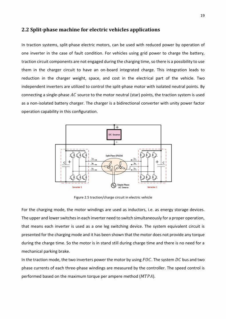
2.2 Split-phase machine for electric vehicles applications

In traction systems, split-phase electric motors, can be used with reduced power by operation of

one inverter in the case of fault condition. For vehicles using grid power to charge the battery,

traction circuit components are not engaged during the charging time, so there is a possibility to use

them in the charger circuit to have an on-board integrated charge. This integration leads to

reduction in the charger weight, space, and cost in the electrical part of the vehicle. Two

independent inverters are utilized to control the split-phase motor with isolated neutral points. By

connecting a single-phase 𝐴𝐶 source to the motor neutral (star) points, the traction system is used

as a non-isolated battery charger. The charger is a bidirectional converter with unity power factor

operation capability in this configuration.

Figure 2.5 traction/charge circuit in electric vehicle

For the charging mode, the motor windings are used as inductors, i.e. as energy storage devices.

The upper and lower switches in each inverter need to switch simultaneously for a proper operation,

that means each inverter is used as a one leg switching device. The system equivalent circuit is

presented for the charging mode and it has been shown that the motor does not provide any torque

during the charge time. So the motor is in stand still during charge time and there is no need for a

mechanical parking brake.

In the traction mode, the two inverters power the motor by using 𝐹𝑂𝐶. The system 𝐷𝐶 bus and two

phase currents of each three-phase windings are measured by the controller. The speed control is

performed based on the maximum torque per ampere method (𝑀𝑇𝑃𝐴).

20

Figure 2.6 equivalent circuit during charge operation

For battery charging, the source is connected to the motor two neutral points, 𝑂1 and 𝑂2 , by a

plug. The motor windings are used as inductors to form a single-phase full-bridge Boost rectifier by

using the available power semiconductors in the inverters. Since the component power rating are

usually high for traction purposes, the charger is a high-power non isolated battery charger. This is

a very efficient and reliable application of split phase electrical machine.

21

2.3 Ship applications: electric and hybrid electric propulsion

Multiphase machines are also used in ship’s power systems, in recent years, electric and hybrid

propulsion is more important due to advantages in electric machine utilization. It’s useful to classify

the systems, in particular how is generated the electrical power and how it is used for electric

propulsion. As for electrical power production we can have:

Diesel-electric propulsion: electrical energy is generated by a diesel prime mover.

Turbo-gas-electric or turbo-electric: when the prime mover is a gas turbine.

Electrochemical generators: in which the electrical energy is generated by an electro-

chemical system which uses hydrogen as fuel and oxygen as oxydising, eventually oxygen

can be withdraw from air.

The other classification is about the propulsion system itself, so it’d be:

𝐷𝐶 motor propulsion systems

Induction motors driven by controlled commutation converters

Synchronous machines driven by cycloconverters

Synchronous machines driven by synchro-converters

Figure 2.7: Principle scheme of the class 𝑇2 tanker

As an example it can be shown the principle circuit of the class 𝑇2 tanker, they were construct in

the world war 2 by USA and they were drive by a large synchronous machine of variable frequency,

from 0 to 60 𝐻𝑧.

22

The prime mover was a steam turbine (today steam turbines are abandoned), and as it can be seen

from the Figure 2.7 it fed all the electric circuit in the ship, while another small steam turbine fed

the excitation of the machine and to all the others 115𝑉 circuits.

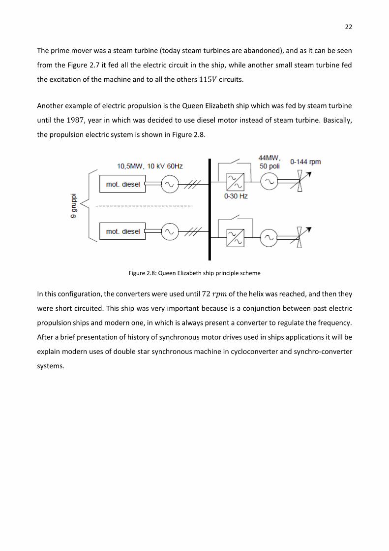
Another example of electric propulsion is the Queen Elizabeth ship which was fed by steam turbine

until the 1987, year in which was decided to use diesel motor instead of steam turbine. Basically,

the propulsion electric system is shown in Figure 2.8.

Figure 2.8: Queen Elizabeth ship principle scheme

In this configuration, the converters were used until 72 𝑟𝑝𝑚 of the helix was reached, and then they

were short circuited. This ship was very important because is a conjunction between past electric

propulsion ships and modern one, in which is always present a converter to regulate the frequency.

After a brief presentation of history of synchronous motor drives used in ships applications it will be

explain modern uses of double star synchronous machine in cycloconverter and synchro-converter

systems.

23

2.3.1 Cycloconverter systems

A cycloconverter is an electrical device which converts single phase or three phase alternating

current into variable magnitude and variable frequency single phase or three phase 𝐴𝐶.

Figure 2.9: block diagram a cycloconverter

Cycloconverters are used in high power applications driving induction and synchronous motors.

They are usually phase-controlled and, traditionally, they use thyristors due to their ease of phase

commutation.

In the case of three phase cycloconverter which is driving a synchronous machine, the system will

be the one presented in Figure 2.10 in which, a standard synchronous machine was used for

propulsion porpuse.

Figure 2.10: three phase cycloconverter

To improve harmonic content of primary current it shown that can be use a 12 pulse bridge which

drives a double star synchronous machine through cycloconverters, so the system can be

represented by the Figure 2.11. The use of a double star synchronous machine (in this case with

independent excitation) improves reliability and power quality. Cycloconverters allow to regulate

24

voltages and currents on the “𝐷𝐶” side of the converters. This solution has a high cost but it is

justified by the high power of the application.

Figure 2.11: double star synchronous machine drives by 12 pulse bridge

2.3.2 Synchronous converter systems

Principle scheme for ship’s propulsion using synchro-converter it is shown in Figure 2.12

Figure 2.12: ship’s propulsion using synchro-converter

In the scheme can be recognize the following devices:

A thyristor rectifier which generates a 𝐷𝐶 system

A thyristor inverter which fed the synchronous motor with a constant magnitude and

variable frequency voltage

Static excitation of the machine

25

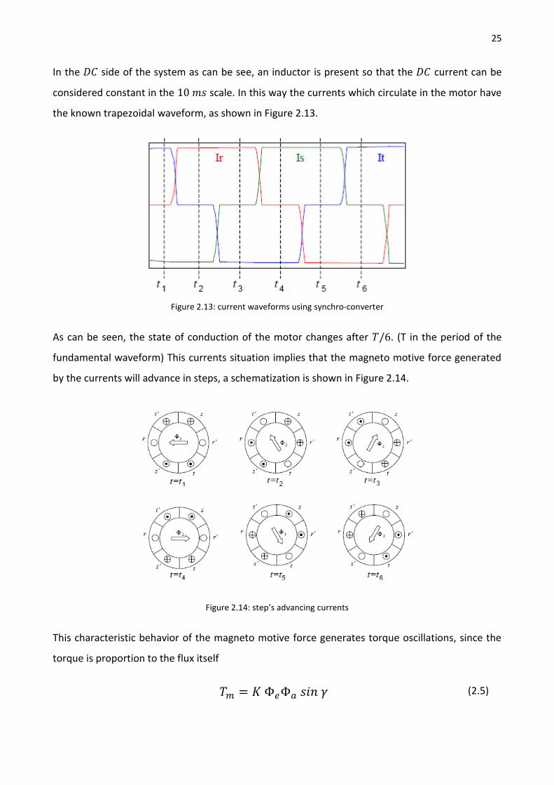
In the 𝐷𝐶 side of the system as can be see, an inductor is present so that the 𝐷𝐶 current can be

considered constant in the 10 𝑚𝑠 scale. In this way the currents which circulate in the motor have

the known trapezoidal waveform, as shown in Figure 2.13.

Figure 2.13: current waveforms using synchro-converter

As can be seen, the state of conduction of the motor changes after 𝑇/6. (T in the period of the

fundamental waveform) This currents situation implies that the magneto motive force generated

by the currents will advance in steps, a schematization is shown in Figure 2.14.

Figure 2.14: step’s advancing currents

This characteristic behavior of the magneto motive force generates torque oscillations, since the

torque is proportion to the flux itself

𝑇𝑚 = 𝐾 Φ𝑒Φ𝑎 𝑠𝑖𝑛 𝛾

(2.5)

26

Where:

Φ𝑒 and Φ𝑎 are excitation and armature flux, respectively

𝛾 is the angle between them

In normal operation Φ𝑒 rotates at nearly constant speed while Φ𝑎 rotates with steps, this is the

reason high torque oscillations are present.

A solution to this problem is the use of a double star synchronous machine with corresponding

windings displaced by 30 degrees, in this way the armature flux will assume 12 positions instead of

6 decreasing sensibly the oscillations of the machine.

Figure 2.15: double star synchronous machine used in synchro-converter fed system

As an example can be seen that in this case was used the double star synchronous machine coupled

with a 12 pulse rectifier, to improve harmonic content of the current draw by the grid.

27

2.4 Locomotive traction system

In the past synchronous motor drives were considered complicated and cumbersome, so

asynchronous drives were preferred. The development of power electronic and in particular of

electrical drives with intermediate 𝐷𝐶 circuit, allowed new development in synchronous machine

drives for traction systems. In particular, in 1982 was experienced the prototype 𝐵𝐵 10004 of

𝑆𝑁𝐹𝐶. The favorable results made possible to understand that synchronous converter systems were

preferable in high power applications.

2.4.1 𝑩𝑩 𝟐𝟔𝟎𝟎𝟎 locomotive system

The locomotive 𝐵𝐵 26000 is an example of traction system in which a double star synchronous

machine was used.

Figure 2.16: principle scheme of one of the two traction motor

The bi-current 𝐵𝐵 26000 called 𝑆𝑌𝐵𝐼𝐶 (syncrones-bicourant), are derive derived from the single

voltage 𝐵𝐵 10004 and they can generate the nominal performances with both supply systems. The

electrical drive is subdivided in two independent sub-drives, their scheme is represented in the two

Figures 2.16 and 2.17. Regulation is carried out with a step down converter. (for example in Figure

2.17 can be seen converter 𝐶𝐻1, used to regulate one of the two traction motor) Converters are

designed for the maximum power, which is, in this case 2800𝑊. The electrical power can be taken

from the 𝐷𝐶 grid through extra-rapid switch or from the ac grid through transformer and single

28

phase mixed bridge. The aim of the two input stages is two supply the nominal voltage which is

1600𝑉.

Figure 2.17: input stage of 𝐵𝐵 26000 locomotive

29

Chapter 3

Double star permanent magnets synchronous

machine

hapter three will present the main focus of the work: the so called double star PMSM.

The chapter is organized in order to understand primarily the construction of the

machine, from which it will be deducted the mathematical model of the machine in the

time domain. Then, from the results obtained in the time domain analysis and using an

appropriate and particular Park’s transformation, the transformed model is obtained and

explained. As it will be seen the variable transformation allows many advantages that will be

exploited for the control system in the chapter related to simulations.

3.1 Description of the machine

The double star synchronous machine is a synchronous multiphase machine in which there are two

sets of stator windings. The magnetic axes of the two stator windings are displaced each other by

𝛼 = 30 𝑑𝑒𝑔 in order to have 𝛼 = 60𝑁⁄ (where 𝑁 is the number of three phase sets) which is the

condition to obtain the so called split-phase configuration. This winding arrangement has different

advantages, such as: possibility of use already existing three phase components, greater power

density and less vibrating mechanical torque. The air gap situation can be represent as shown in the

Figure 3.1. The rotor is the same as its three phase counterparts and it is made with permanent

magnets, in particular interior permanent magnets (𝐼𝑃𝑀) and surface permanent magnets (𝑆𝑃𝑀)

manufacture techniques are used.

c

30

Interior permanent magnet (𝐼𝑃𝑀) machines are widely used taking advantage of the additional

torque component due to reluctance dependence on rotor position; such dependence obviously

affects the winding inductances, introducing a relevant complication in the case of double star.

Figure 3.1 windings arrangement in double star synchronous machine

The inherent advantage of this machine type is the elimination of the sixth harmonic torque

pulsation. Furthermore, using two three-phase sets instead of one increases the redundancy of the

system, as it was seen in chapter 2. Park’s transformation is generally applied to three phase

machines to model the machine using the rotor reference frame, which, especially for 𝐼𝑃𝑀

machines, is an important tool to eliminate the rotor angle dependency of inductances. From the

control design point of view, such simplifications are usually acceptable since non-idealities can be

considered as disturbances, but from the simulation point of view, the model may be oversimplified,

and thus, important phenomena may not become visible.

The electromagnetic coupling between the winding sets makes the modeling of double-star

machines more complex compared with conventional three-phase machines where such a coupling,

obviously, does not exist.

3.1.1 Rotor configurations

The rotor is made by permanent magnet materials. In recent years the interest in this materials is

improved and this made possible to have better materials at relative low cost, this is the reason why

𝑃𝑀𝑆𝑀 are nowadays used in much more applications with respect to the past.

The earliest manufactured magnet materials were hardened steel. Magnets made from steel were

easily magnetized. However, they could hold very low energy and it was easy to demagnetize. In

31

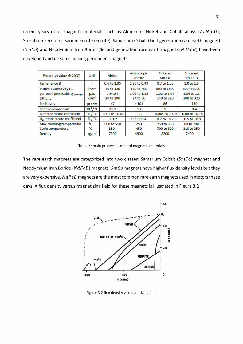
recent years other magnetic materials such as Aluminum Nickel and Cobalt alloys (𝐴𝐿𝑁𝐼𝐶𝑂),

Strontium Ferrite or Barium Ferrite (Ferrite), Samarium Cobalt (First generation rare earth magnet)

(𝑆𝑚𝐶𝑜) and Neodymium Iron-Boron (Second generation rare earth magnet) (𝑁𝑑𝐹𝑒𝐵) have been

developed and used for making permanent magnets.

Table 3: main properties of hard magnetic materials

The rare earth magnets are categorized into two classes: Samarium Cobalt (𝑆𝑚𝐶𝑜) magnets and

Neodymium Iron Boride (𝑁𝑑𝐹𝑒𝐵) magnets. 𝑆𝑚𝐶𝑜 magnets have higher flux density levels but they

are very expensive. 𝑁𝑑𝐹𝑒𝐵 magnets are the most common rare earth magnets used in motors these

days. A flux density versus magnetizing field for these magnets is illustrated in Figure 3.2

Figure 3.2 flux density vs magnetizing field

32

Hard magnetic materials are characterized by a broad main hysteresis loop and by a high coercitivity

(for this reason they are called “hard” materials); on the contrary, iron and most of iron alloys have

a narrow main hysteresis loop, and a low coercivity (for this reason they are called “soft” materials).

This property of the hard materials implies a high value of hysteresis losses (since, when the supply

delivers a 𝐷𝐶 current, the area of the hysteresis loop equals the hysteresis loss).

Actually, this is not a trouble, since in normal operating conditions, 𝑃𝑀𝑠 work with static fields (not

with 𝐴𝐶 fields), thus the 𝑃𝑀 material do not travel along the hysteresis loop, and the hysteresis

losses do not occur.

Figure 3.3: working point in hard magnetic materials

Instead, the useful consequence of a broad hysteresis loop is that when such a material is inserted

in a magnetic circuit, the working point on the magnetization curve has a high flux density, therefore

such material can be used as a flux source.

On the contrary, if a soft material is inserted in a magnetic circuit, the working point on the

magnetization curve has a very low flux density, therefore a soft material cannot be used as a flux

source. This property is demonstrated if the working point is obtained by a graphical intersection

between the magnetic characteristic of the flux source (the 𝐵 − 𝐻 curve of the 𝑃𝑀 in the 2𝑛𝑑

quadrant of 𝐵 − 𝐻 plane) and the magnetic characteristic of the magnetic, passive load (a straight

line, passing through origin of 𝐵 − 𝐻 plane, with a negative slope).

33

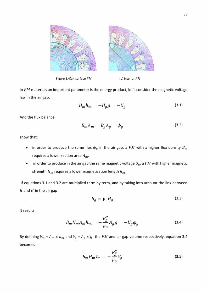
Figure 3.4(a): surface 𝑃𝑀 (b) interior 𝑃𝑀

In 𝑃𝑀 materials an important parameter is the energy product, let’s consider the magnetic voltage

law in the air gap:

𝐻𝑚ℎ𝑚 = −𝐻𝑔𝑔 = −𝑈𝑔

(3.1)

And the flux balance:

𝐵𝑚𝐴𝑚 = 𝐵𝑔𝐴𝑔 = 𝜙𝑔

(3.2)

show that:

in order to produce the same flux 𝜙𝑔 in the air gap, a 𝑃𝑀 with a higher flux density 𝐵𝑚

requires a lower section area 𝐴𝑚.

in order to produce in the air gap the same magnetic voltage 𝑈𝑔, a 𝑃𝑀 with higher magnetic

strength 𝐻𝑚 requires a lower magnetization length ℎ𝑚

If equations 3.1 and 3.2 are multiplied term by term, and by taking into account the link between

𝐵 and 𝐻 in the air gap

𝐵𝑔 = µ0𝐻𝑔

(3.3)

It results

𝐵𝑚𝐻𝑚𝐴𝑚ℎ𝑚 = −

𝐵𝑔2

𝜇0𝐴𝑔𝑔 = −𝑈𝑔𝜙𝑔 (3.4)

By defining 𝑉𝑚 = 𝐴𝑚 𝑥 ℎ𝑚 and 𝑉𝑔 = 𝐴𝑔 𝑥 𝑔 the 𝑃𝑀 and air gap volume respectively, equation 3.4

becomes

𝐵𝑚𝐻𝑚𝑉𝑚 = −

𝐵𝑔2

𝜇0𝑉𝑔 (3.5)

34

And solving for 𝑉𝑚:

The minus sign in equation 3.6 occurs because the 𝑃𝑀 working magnetic strength 𝐻𝑚 is negative,

due to the operation in the 2𝑛𝑑 quadrant. Equation 3.6 shows that, if the air gap volume 𝑉𝑔 and flux

density 𝐵𝑔 are defined, the 𝑃𝑀 volume 𝑉𝑚 is in inverse proportion with respect to the product

𝐵𝑚𝑥 𝐻𝑚: this quantity is an energy per unit volume 𝑊 𝑚3⁄ , and for this reason it is called energy

product. Thus, it seems to be advisable that the 𝑃𝑀 working point be in that portion of the

characteristic where the product 𝐵𝑚𝑥 𝐻𝑚 assumes its maximum value, since in this point (with fixed

value of 𝐵𝑔 , 𝐻𝑔, 𝑔, 𝐴𝑔) the 𝑃𝑀 volume has a minimum. In a similar way, since the energy stored in

the air gap is expressed by:

𝑊𝑔 = −

1

2

𝐵𝑔2

𝜇0𝐴𝑔𝑔 = −

1

2𝐵𝑚𝐻𝑚𝑉𝑚

(3.7)

if the 𝑃𝑀 volume is defined, the air gap energy is the higher, the higher is the energy product

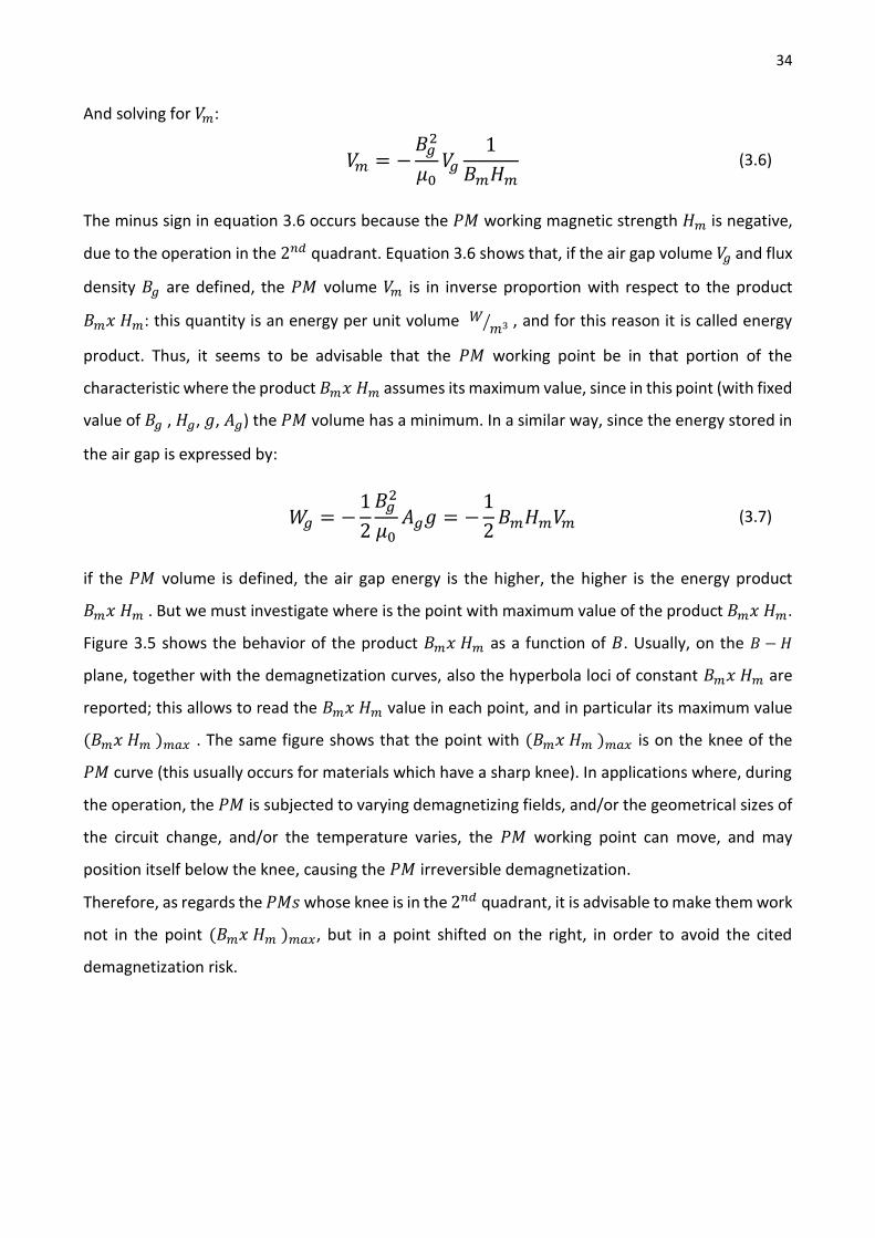
𝐵𝑚𝑥 𝐻𝑚 . But we must investigate where is the point with maximum value of the product 𝐵𝑚𝑥 𝐻𝑚.

Figure 3.5 shows the behavior of the product 𝐵𝑚𝑥 𝐻𝑚 as a function of 𝐵. Usually, on the 𝐵 − 𝐻

plane, together with the demagnetization curves, also the hyperbola loci of constant 𝐵𝑚𝑥 𝐻𝑚 are

reported; this allows to read the 𝐵𝑚𝑥 𝐻𝑚 value in each point, and in particular its maximum value

(𝐵𝑚𝑥 𝐻𝑚 )𝑚𝑎𝑥 . The same figure shows that the point with (𝐵𝑚𝑥 𝐻𝑚 )𝑚𝑎𝑥 is on the knee of the

𝑃𝑀 curve (this usually occurs for materials which have a sharp knee). In applications where, during

the operation, the 𝑃𝑀 is subjected to varying demagnetizing fields, and/or the geometrical sizes of

the circuit change, and/or the temperature varies, the 𝑃𝑀 working point can move, and may

position itself below the knee, causing the 𝑃𝑀 irreversible demagnetization.

Therefore, as regards the 𝑃𝑀𝑠 whose knee is in the 2𝑛𝑑 quadrant, it is advisable to make them work

not in the point (𝐵𝑚𝑥 𝐻𝑚 )𝑚𝑎𝑥, but in a point shifted on the right, in order to avoid the cited

demagnetization risk.

𝑉𝑚 = −

𝐵𝑔2

𝜇0𝑉𝑔

1

𝐵𝑚𝐻𝑚 (3.6)

35

Figure 3.5 maximum energy product

𝑃𝑀 motors are broadly classified by the direction of the field flux. The first field flux classification is

radial field motor meaning that the flux is along the radius of the motor. The second is axial field

motor meaning that the flux is perpendicular to the radius of the motor. Radial field flux is most

commonly used in motors and axial field flux have become a topic of interest for study and used in

a few applications.

𝑃𝑀 motors are classified on the basis of the flux density distribution and the shape of current

excitation. They are 𝑃𝑀𝑆𝑀 and 𝑃𝑀 brushless motors (𝐵𝐷𝐶𝑀). The 𝑃𝑀𝑆𝑀 has a sinusoidal-shaped

back 𝐸𝑀𝐹 and is designed to develop sinusoidal back 𝐸𝑀𝐹 waveforms. They have the following

features:

Sinusoidal distribution of magnet flux in the air gap

Sinusoidal current waveforms

Sinusoidal distribution of stator conductors.

𝐵𝐷𝐶𝑀 has a trapezoidal-shaped back 𝐸𝑀𝐹 and is designed to develop trapezoidal back

𝐸𝑀𝐹 waveforms. They have the following features:

Rectangular distribution of magnet flux in the air gap

Rectangular current waveform

Concentrated stator windings.

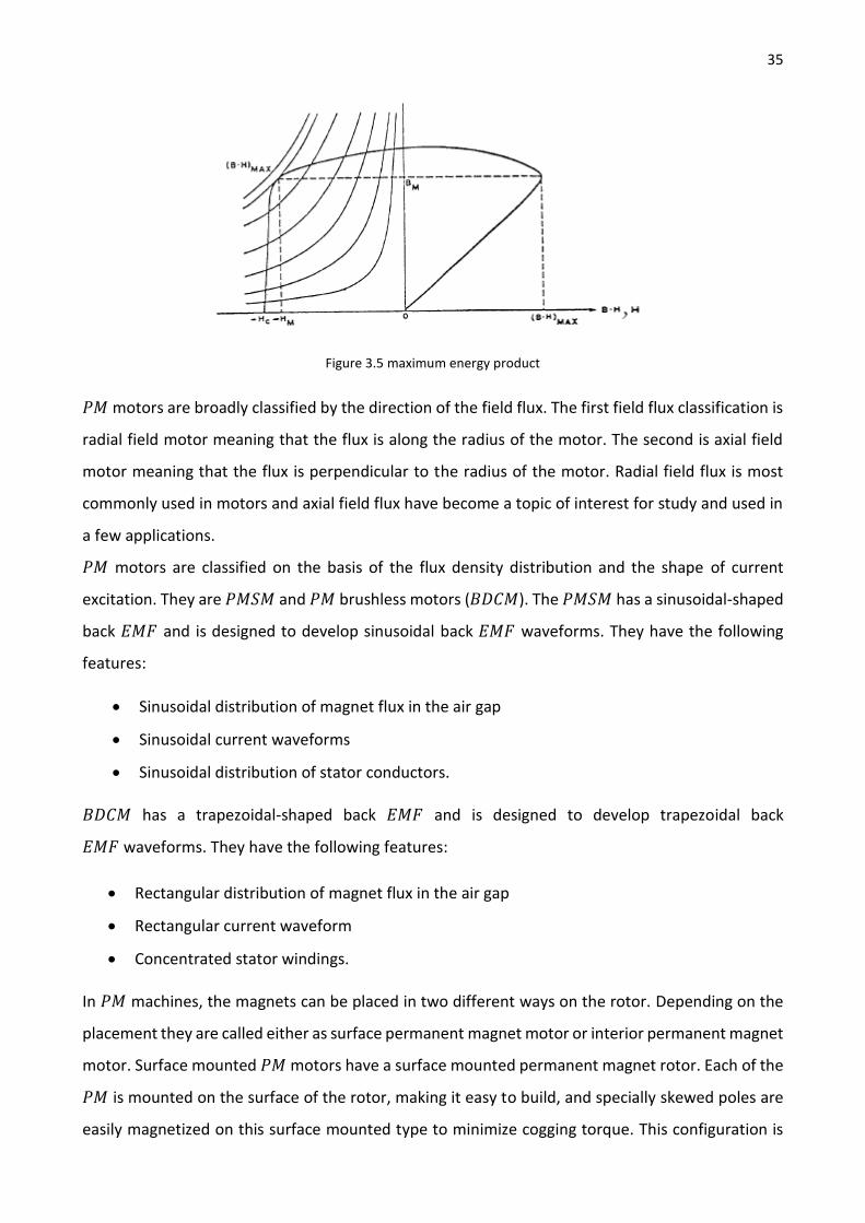
In 𝑃𝑀 machines, the magnets can be placed in two different ways on the rotor. Depending on the

placement they are called either as surface permanent magnet motor or interior permanent magnet

motor. Surface mounted 𝑃𝑀 motors have a surface mounted permanent magnet rotor. Each of the

𝑃𝑀 is mounted on the surface of the rotor, making it easy to build, and specially skewed poles are

easily magnetized on this surface mounted type to minimize cogging torque. This configuration is

36

used for low speed applications because of the limitation that the magnets will fly apart during high-

speed operations. These motors are considered to have small saliency, thus having practically equal

inductances in both axes.

The permeability of the permanent magnet is almost that of the air, thus the magnetic material

becoming an extension of the air gap. For a surface permanent magnet motor 𝐿𝑑 = 𝐿𝑞. The rotor

has an iron core that may be solid or may be made of punched laminations for simplicity in

manufacturing. Thin permanent magnets are mounted on the surface of this core using adhesives.

Alternating magnets of the opposite magnetization direction produce radially directed flux density

across the air gap. This flux density then reacts with currents in windings placed in slots on the inner

surface of the stator to produce torque. Figure 2.3 shows the placement of the magnet.

Figure 3.6(a): surface permanent magnets (b) interior permanent magnets

Interior 𝑃𝑀 motors have interior mounted permanent magnet rotor as shown in figure 2.4. Each

permanent magnet is mounted inside the rotor. It is not as common as the surface mounted type

but it is a good candidate for high-speed operation. There is inductance variation for this type of

rotor because the permanent magnet part is equivalent to air in the magnetic circuit calculation.

These motors are considered to have saliency with 𝑞-axis inductance greater than the 𝑑-axis

inductance (𝐿𝑑 > 𝐿𝑞).

37

3.1.2 No load back EMF

The no-load back-𝐸𝑀𝐹 waveform in 𝑃𝑀 synchronous machines depends on the rotor electrical

rotational speed 𝜔𝑒 and the Ψ𝑃𝑀 flux produced by the 𝑃𝑀𝑠. Commonly, Ψ𝑃𝑀 is assumed constant

in transformed models. In the steady state, 𝜔𝑒 can be assumed to be constant with a negligible

error. Assuming both the values constant results in sinusoidal voltage waveforms. However,

assuming Ψ𝑃𝑀 constant requires the air-gap flux density distribution to be sinusoidal. It is worth

mentioning that the harmonics in the no-load flux linkage can be taken into account in transformed

models also.

Generally, the voltage induced in the winding is given by:

𝐸0 = −

𝑑Ψ𝑃𝑀

𝑑𝑡 (3.8)

Where Ψ𝑃𝑀 is the flux linkage of the winding. The parameters having the greatest effect on the

induced voltage are the winding factor, the number of turns of the coil, the cross-sectional area of

the coil, and the flux density in the air gap.

In 𝑃𝑀 machines, the air gap flux density is obviously affected by the magnet configuration and the

magnetization direction, as well as by the stator geometry, e.g. stator slotting, which can be taken

into account by an analytical method, based on the determination of the air-gap magneto motive

force and the flux path permeance function. Besides being rather complex, such a model requires

(similarly as an 𝐹𝐸 model) the knowledge of the geometry details of the machine and the material

characteristics. In addition to the stator slotting, the winding layout has an important impact on the

harmonics generated in the back 𝐸𝑀𝐹.

The greatest winding factor for the fundamental wave in the case of a conventional three phase

machine is achievable with a full-pitch winding layout. As a drawback, the winding factors of the

harmonics (especially the 5𝑡ℎ and 7𝑡ℎ) increase as well. The double-star full-pitch windings generally

exhibit even higher harmonic components. As a benefit, higher voltage is obtained, the same air gap

flux being maintained, even if with a greater harmonic content.

38

3.1.3 Hypotheses

In developing the mathematical model, the following assumptions are made:

The set of three-phase stator winding is symmetrical.

The capacitance of all the windings can be neglected.

Each of the distributed windings may be represented by a concentrated winding.

The change in the inductance of the stator windings due to rotor position is sinusoidal

and does not contain higher harmonics.

Hysteresis loss and eddy current losses are ignored.

The magnetic circuits are linear (not saturated) and the inductance values do not

depend on the current.

3.2 Phase variable model

3.2.1 model Structure

The phase-variable model can be written in the following vector notation:

𝑽 = 𝑹𝑠𝑰 + 𝑝𝚿 (3.9)

where is 𝑹𝒔the stator winding resistance matrix, 𝑝 is the time derivative operator, and 𝚿 is the flux

linkage vector composed of the no-load flux Ψ𝑃𝑀 generated by the 𝑃𝑀𝑠 and the armature reaction

as follows:

𝚿 = 𝑳(𝜽)𝑰 + 𝚿𝑷𝑴 (3.10)

The vectors 𝑽 ,𝑰 , 𝚿 and 𝚿𝑷𝑴 are in the form:

𝒇 = [ 𝑓𝑎1

𝑓𝑏1 𝑓𝑐1 𝑓𝑎2 𝑓𝑏2 𝑓𝑐2

]𝑇 (3.11)

Currents are selected as state variables and the equations to be solve are derived from the system

of equation 3.9, obtaining:

p𝑰 = 𝑳(𝜽)−𝟏(𝑽 − p𝚿𝑷𝑴 − 𝑹𝒔𝑰 + p𝑳(𝜽) ∙ 𝑰)

(3.12)

39

3.2.2 Inductances

The dependence of the self- and mutual inductances on rotor position 𝜃 is generally conveniently

expressed by Fourier expansions. For example, a general equation defining a self-inductance and

taking into account higher order harmonics, can be written as:

𝐿𝑖(𝜃) = 𝐿𝑖0 + ∑ 𝐿𝑖2𝑛

∞

𝑛=1

cos (2𝑛𝜃𝑖 + 𝜑𝑖𝑛) (3.13)

where the subscript 𝑖 denotes the 𝑖𝑡ℎ winding ( 𝑖 = 𝑎1, …,𝑐2 ), 𝐿𝑖0 is the average value, 𝐿𝑖2𝑛 is the

coefficient of inductance harmonics (2𝑛𝑑, 4𝑡ℎ, 6𝑡ℎ, …), and 𝜑𝑖𝑛 is the displacement angle of the

corresponding harmonic component. A similar equation can be written to define the mutual

inductance as well:

𝑀𝑖𝑗(𝜃) = 𝑀𝑖𝑗0 + ∑ 𝑀𝑖𝑗2𝑛

∞

𝑛=1

cos (𝑛(𝜃𝑖 + 𝜃𝑗) + 𝜑𝑖𝑛) (3.14)

where the subscript 𝑖 , 𝑗 denotes the coupling between the 𝑖𝑡ℎand 𝑗𝑡ℎ windings (𝑖 , 𝑗 = 𝑎1, …, 𝑐2,

𝑖 ≠ 𝑗 ).

3.2.3 inductance waveforms

In general, when an electrical machine is modeled using Park’s transformation, the 𝑑 − 𝑞 axes

inductances are considered constant, meaning that the higher-order inductance harmonics are

neglected. The fundamental waveforms are defined by equations 3.13 and 3.14 with 𝑛 = 1.

Using the inbuilt post-processing procedures of the Maxwell 𝐹𝐸𝑀 software, the inductance

waveforms that also include higher-order harmonics can be obtained. Figure 3.7 shows the work

made in [3], in which inductance waveforms related to coil 𝑎1 are illustrated. The relative amounts

of harmonic components with respect to the fundamental one are shown in Table 4. According to

Table 4, significant amounts of harmonics, especially even harmonics, are present. The presence of

even harmonics is clearly visible also in Figure 3.7 because the negative and positive half-cycles are

not symmetrical. Particularly, the values of the 4𝑡ℎ-order inductance coefficients (𝑛 = 2) are

significantly high.

40

Table 4: value of inductance harmonics

Figure 3.7: inductance waveforms

3.2.4 Inductance matrix

Considering only the first inductance harmonic equations 3.13 and 3.14 become:

𝐿𝑖(𝜃) = 𝐿𝑖0 + 𝐿𝑖0 cos (2𝑛𝜃𝑖) (3.15)

𝑀𝑖𝑗(𝜃) = 𝑀𝑖𝑗0 + 𝑀𝑖𝑗0 cos (𝜃𝑖 + 𝜃𝑗)

(3.16)

It can be shown that the inductance matrix is made in this way:

41

𝑳(𝜃) = [

𝑳1(𝜃) 𝑴12(𝜃)𝑴21(𝜃) 𝑳2(𝜃)

] (3.15)

It is a 6𝑋6 full matrix in which we can recognize four main matrices, in particular we have:

𝑳1(𝜃): matrix associates with the first three phase winding, it expresses its self and mutual

inductance.

𝑳2(𝜃): matrix associated with the second three phase winding.

𝑴12(𝜃) ,𝑴21(𝜃): these two matrices represent the effect of one three phase winding on

the other.

Each of them are 3𝑋3 full matrices where every single term is 𝜃 dependent, later will be shown that

using Park’s transformation we can simplify these matrices and eliminate the rotor position

dependence.

For the sake of clarity can be shown the complete matrix:

[

𝐿𝑎1(𝜃) 𝑀𝑎1𝑏1

(𝜃) 𝑀𝑎1𝑐1(𝜃)

𝑀𝑏1𝑎1(𝜃) 𝐿𝑏1(𝜃) 𝑀𝑏1𝑐1(𝜃)𝑀𝑐1𝑎1(𝜃) 𝑀𝑐1𝑏1(𝜃) 𝐿𝑐1(𝜃)

𝑀𝑎1𝑎2(𝜃) 𝑀𝑎1𝑏2(𝜃) 𝑀𝑎1𝑐2(𝜃)𝑀𝑏1𝑎2(𝜃) 𝑀𝑏1𝑏2(𝜃) 𝑀𝑏1𝑐2(𝜃)𝑀𝑐1𝑎2(𝜃) 𝑀𝑐1𝑏2(𝜃) 𝑀𝑐1𝑐2(𝜃)

𝑀𝑎2𝑎1(𝜃) 𝑀𝑎2𝑏1(𝜃) 𝑀𝑎2𝑐1(𝜃)𝑀𝑏2𝑎1(𝜃) 𝑀𝑏2𝑏1(𝜃) 𝑀𝑏2𝑐1(𝜃)𝑀𝑐2𝑎1(𝜃) 𝑀𝑐2𝑏1(𝜃) 𝑀𝑐2𝑐1(𝜃)

𝐿𝑎2(𝜃) 𝑀𝑎2𝑏2(𝜃) 𝑀𝑎2𝑐2(𝜃)𝑀𝑏2𝑎2(𝜃) 𝐿𝑏2(𝜃) 𝑀𝑏2𝑐2(𝜃)𝑀𝑐2𝑎2(𝜃) 𝑀𝑐2𝑏2(𝜃) 𝐿𝑐2(𝜃) ]

(3.16)

In which it can be recognize the four main matrices presented earlier.

3.2.5 Electromagnetic torque

The torque equation can be derived starting from the energy stored in the magnetic fields and

defined as follow:

𝑇𝑒 = 𝑛𝑝

(12

𝑰𝑇 𝜕𝑳𝜕𝑡

𝑰 + 𝑰𝑇 𝜕𝜕𝑡

𝚿𝑃𝑀)

𝜔𝑒

(3.17)

Where 𝑛𝑝 is the number of pole pairs.

42

3.3 Transformed variables model

3.3.1 Introduction

General tools for multiphase machine modeling have been developed in the first half of the 20𝑡ℎ

century. The well-known space vector and 𝑑 − 𝑞 models of three-phase machines are only

particular cases of the universal 𝑛-phase machine models. Since the phase-variable model of a

physical multiphase machine gets transformed using a mathematical transformation, the number

of variables before and after transformation must remain the same.

This means that an 𝑛-phase machine will have 𝑛 new stator current (stator voltage, stator flux)

components after the transformation. If a machine is with sinusoidal-field distribution, standard

modeling assumptions apply and only the first harmonic of inductance terms exists in the phase-

variable model. Application of the decoupling (Park’s) transformation produces a set of 𝑛 equations.

The transformation will eliminate the dependence on the rotor position, simplifying the

modelization of the machine and the design of the drive.

3.3.2 Park transformation matrix

Park’s transformation for a three-phase system with no neutral connection is defined by the 2 × 3

matrix as:

𝑻𝑝(𝛿) = √2

3(

𝑐𝑜𝑠(𝛿) 𝑐𝑜𝑠 (𝛿 −2𝜋

3) 𝑐𝑜𝑠 (𝛿 +

2𝜋

3)

−𝑠𝑖𝑛(𝛿) −𝑠𝑖𝑛 (𝛿 −2𝜋

3) −𝑠𝑖𝑛 (𝛿 +

2𝜋

3)

)

(3.18)

The transformation matrix that transforms the phase variables, for instance, the 𝑳(𝜃) 6𝑥6 matrix,

into the 𝑑– 𝑞 reference frame is composed by two Park’s transformation matrices and can be

expressed as:

𝑻1(𝜃) = (

𝑻𝑝(𝜃 + α) 𝟎2,3

𝟎2,3 𝑻𝑝(𝜃 − α)) (3.19)

where 𝟎𝑖,𝑗 is a null matrix with 𝑖 rows and 𝑗 columns. Applying matrix 3.19 to 3.16, the resulting

matrix 𝑳𝑇1, related to two couples of orthogonal windings 𝑑∗ − 𝑞∗ and 𝑑∗∗ − 𝑞∗∗ , is given by:

43

𝑳𝑇1= 𝑻1(𝜃)𝑳(𝜃)𝑻1

𝑇(𝜃) (3.20)

𝑳𝑇1

= (𝑳𝑑𝑞∗ 𝑴𝑑𝑞∗

𝑴𝑑𝑞∗ 𝑳𝑑𝑞∗∗)

(3.21)

Where

𝑳𝑑𝑞∗ = 𝑳𝑑𝑞∗∗ = (𝐿𝑑∗ 00 𝐿𝑞∗

)

𝑴𝑑𝑞∗ = (𝑀𝑑∗ 00 𝑀𝑞∗

)

And

𝐿𝑑∗ = 𝐿𝑠0+

𝐿𝑠2

2− 𝑀𝑠2

+ 𝑀𝑠2

𝐿𝑞∗ = 𝐿𝑠0−

𝐿𝑠2

2− 𝑀𝑠2

− 𝑀𝑠2

𝑀𝑑∗ =1

2(3𝑀𝑚0

+ 𝑀𝑚2)

𝑀𝑞∗ =1

2(3𝑀𝑚0

− 𝑀𝑚2)

The complete 𝑳𝑇1 matrix is shown:

𝑳𝑇1=

(

(𝐿𝑑∗ 00 𝐿𝑞∗

) (𝑀𝑑∗ 00 𝑀𝑞∗

)

(𝑀𝑑∗ 00 𝑀𝑞∗

) (𝐿𝑑∗ 00 𝐿𝑞∗

))

(3.22)

With 𝑳𝑇1 not being a diagonal matrix, the transformed winding couples 𝑑∗ − 𝑞∗ and 𝑑∗∗ − 𝑞∗∗ are

mutually coupled with respect to each other. The matrix of the further transformation required to

eliminate such a coupling can be found by diagonalizing 𝑳𝑇1. With a suitable rearrangement of rows

and columns, the transformation matrix 𝑻2 to the final decoupled 𝑑1 – 𝑞1 and 𝑑2 – 𝑞2 reference

frames (also referred to as 𝑑 – 𝑞 reference frames) is obtained:

44

𝑻2 = 𝑘 (

1 00 1

1 00 1

0 1−1 0

0 −11 0

)

(3.23)

where the orthonormalization coefficient 𝑘 = 1√2

⁄ is introduced to enable the power to be

invariant. Application of matrix 3.23 to 3.22 yields:

𝑳𝑇2=

(

𝐿𝑑10

0 𝐿𝑞1

0 00 0

0 00 0

𝐿𝑑20

0 𝐿𝑞2)

(3.24)

where the inductances are defined by

𝐿𝑑! = 𝐿𝑑∗ + 𝑀𝑑∗

𝐿𝑞1= 𝐿𝑑∗ + 𝑀𝑞∗

𝐿𝑑2= 𝐿𝑞∗ − 𝑀𝑞∗

𝐿𝑞2= 𝐿𝑑∗ − 𝑀𝑑∗

Finally, by combining matrix 3.19 with 3.23, the whole transformation results in

𝑻3(𝜃) = (𝑻𝑝(𝜃 + α) 𝑻𝑝(𝜃 − α)

𝑻𝑝 (𝜃 + α +𝜋

2) 𝑻𝑝 (𝜃 − α −

𝜋

2))

(3.25)

Figure 3.8: graphical representation of the transformation

45

It is worth mentioning that 𝑳𝑇2 is directly derivable by the application of 𝑻3(𝜃). The proposed

transformation eliminates, like Park’s one, the triplex harmonics from the transformed quantities,

although they are generally not relevant in symmetric three-phase systems.

3.3.3 Transformed model

Starting from the phase variable model:

𝒗𝑠 = 𝑹𝑠𝒊𝑠 + 𝑝𝚿 (3.9)

𝒗𝑠 = 𝑹𝑠𝒊𝑠 + 𝑳(𝜃)𝑝𝒊𝑠 + 𝑝𝑳(𝜃)𝒊𝑠 + 𝒆 (3.9a)

Applying 𝑻3(𝜃) matrix it can be obtained:

𝒗𝑑𝑞 = 𝑹𝑠𝒊𝑑𝑞 + 𝑳𝑑𝑞𝑝𝒊𝑑𝑞 + 𝜔𝑚𝑱𝑳𝑑𝑞𝒊𝑑𝑞 + 𝒆𝑑𝑞

(3.26)

Where:

𝑱 = (

0 −11 0

0 00 0

0 00 0

0 −11 0

)

(3.27)

In expanded form the equation will have this form.

𝑣𝑑1= 𝑅𝑠𝑖𝑑1

+ 𝐿𝑑1𝑝𝑖𝑑1

− 𝜔𝑒𝐿𝑞1𝑖𝑞1

𝑣𝑞1

= 𝑅𝑠𝑖𝑞1+ 𝐿𝑞1

𝑝𝑖𝑞1+ 𝜔𝑒𝐿𝑑1

𝑖𝑑1+ 𝜔𝑒Ψ𝑃𝑀

𝑣𝑑2

= 𝑅𝑠𝑖𝑑2+ 𝐿𝑑1

𝑝𝑖𝑑2− 𝜔𝑒𝐿𝑞2

𝑖𝑞2

𝑣𝑞2= 𝑅𝑠𝑖𝑞2

+ 𝐿𝑞2𝑝𝑖𝑞2

+ 𝜔𝑒𝐿𝑑2𝑖𝑑2

(3.28)

The model using currents as state variable can be write:

𝑝𝑖𝑑1

=1

𝐿𝑑1

(𝑣𝑑1− 𝑅𝑠𝑖𝑑1

+ 𝜔𝑒𝐿𝑞1𝑖𝑞1

)

𝑝𝑖𝑞1=

1

𝐿𝑄1

(𝑣𝑞1− 𝑅𝑠𝑖𝑞1

− 𝜔𝑒𝐿𝑑1𝑖𝑑1

− 𝜔𝑒𝛹𝑃𝑀)

𝑝𝑖𝑑2=

1

𝐿𝑑2

(𝑣𝑑2− 𝑅𝑠𝑖𝑑2

+ 𝜔𝑒𝐿𝑞2𝑖𝑞2

)

(3.29)

46

𝑝𝑖𝑞2=

1

𝐿𝑞2

(𝑣𝑞2− 𝑅𝑠𝑖𝑞2

− 𝜔𝑒𝐿𝑑2𝑖𝑑2

)

And it is necessary to add the mechanical equation as well, which is, in its simplified form:

𝑝𝜔𝑒 =

𝑛𝑝

𝐽(𝑇𝑒 − 𝑇𝑚)

(3.30)

3.3.4 Electromagnetic torque

The equation for the electromagnetic torque is derived starting from the instantaneous power:

𝑃(𝑡) = 𝑣𝑑1𝑖𝑑1

+ 𝑣𝑞1𝑖𝑞1

+ 𝑣𝑑2𝑖𝑑2


(3.31)

In the steady state and neglecting the resistive voltage drop, the equation 3.26 becomes:

𝒗𝑑𝑞 = 𝒆𝑑𝑞 − 𝜔𝑚𝑱𝑳𝑑𝑞𝒊𝑑𝑞

(3.32)

Combining 3.31 and 3.32 and dividing 𝑃(𝑡) by the angular speed 𝜔𝑚 =𝜔𝑒

𝑛𝑝⁄ the electromagnetic

torque is obtained:

𝑇𝑒 = 𝑛𝑝(𝑖𝑞1Ψ𝑑1

∗ + 𝑖𝑞2Ψ𝑞2

∗ − 𝑖𝑑1Ψ𝑃𝑀,𝑞1

− 𝑖𝑑2Ψ𝑃𝑀,𝑞2

)

(3.33)

With

Ψ𝑑1

∗ = 𝑖𝑑1(𝐿𝑞1

− 𝐿𝑑1) + Ψ𝑃𝑀,𝑑1

Ψ𝑑2

∗ = 𝑖𝑑2(𝐿𝑑2

− 𝐿𝑞2) + Ψ𝑃𝑀,𝑑2

If 𝑃𝑀 flux harmonics are negligible but the fundamental one, 𝐿𝑑2= 𝐿𝑞2

and taking into account

inductance expression, 𝑀𝑚2= 𝐿𝑠2

+ 2𝑀𝑠2 , equation 3.33 simplifies to

𝑇𝑒 = 𝑛𝑝Ψ𝑑1

∗ 𝑖𝑞1= 𝑛𝑝[Ψ𝑃𝑀𝑖𝑞1

+ 𝑖𝑞1𝑖𝑑1

(𝐿𝑑1− 𝐿𝑞1

)]

(3.34)

recalling the simplified expression of the electromagnetic torque of variable-reluctance three-phase

machines.

The torque is made by two contributions, the first one is the interaction between the current on the

𝑞1 axis of the first winding set with the permanent magnet flux on the same axis and it is an

47

alignment torque, proportional to currents and flux. The second term is due to permanent magnets

shape and it is a reluctance torque contribution, 𝐼𝑃𝑀 machines are hybrid machines, meaning that

the total torque is a combination of isotropic 𝑃𝑀𝑆𝑀 and a reluctance synchronous machine.

3.3.5 Equivalent circuit

To show the machine equivalent circuit it can be take into account the founded 𝑑 − 𝑞 decoupled

system.




𝑣𝑞1




𝑣𝑑2



𝑖𝑞2




(3.28)

As can be seen the two axes are divided, to obtain two equivalent circuit, in which is possible to

recognize the 𝐹𝐸𝑀 contributes.

Figure 3.9: 𝑑-axis equivalent circuit

Figure 3.10: 𝑞-axis equivalent circuit

49

Chapter 4

control strategies

n the next chapter wind turbine systems and means to control grid side converters will be

presented. The aim of the brief presentation of wind turbine systems is to give the needed

information to understand the control problem, such as: input variable, aim of the control

system, desire value of output variables. Additionally, classical PMSM topologies are presented

along with the studied structure which is, as already said, not yet used in this kind of generation

systems.

4.1 Wind turbines general characteristics

4.1.1 Generalities

There are horizontal and vertical axes wind turbine, the most installed are the horizontal axes wind

turbines and the ones studied in this work. The power density of the wind is not very high, so to

have interesting powers the only mean is to have a high swept area by the blades. A wind turbine

needs a minimal speed of 3 − 5 𝑚/𝑠 (cut-in) to deliver power to the grid instead the rated power

is delivered when the wind speed reach 12 − 14 𝑚/𝑠. When the speed is higher of 25 𝑚/𝑠 (cut-off)

the turbine is stopped for safety reasons.

To the air flow can be associated a power (considering air flow with constant speed 𝑣 and

perpendicular with respect to section ):

𝑃𝑤 =

𝑑

𝑑𝑡(1

2𝑚𝑣2) =

1

2𝑣2

𝑑𝑚

𝑑𝑡=

1

2𝑣2(𝜌𝑆𝑣) =

1

2𝜌𝑆𝑣3 (4.1)

I

50

The extraction of power from the air flow implies that the air will slow down and that its section

increases. The power can’t be extracted completely from the air flow otherwise the air would stop

in the considered section.

Figure 4.1: (a) wind turbine blades and relative speeds (b) air flow

The maximum power which can be extracted from the air flow is:

𝑃∗ =

1

2𝜌𝑆𝑣∗(𝑣1

2 − 𝑣2∗2) =

1

2𝜌𝑆

2

3𝑣1 (

8

9𝑣1

2) =1

2𝜌𝑆

16

27𝑣1

3 (4.2)

The value 16/27 = 0.593 is the Betz’ limit. The maximum power which can be converted from the

undisturbed flow is about the 60%.

In practice the real extracted power is 60 − 70 % of this theoretical value.

Power is:

proportional to 𝑆 i.e. 𝐷𝑏2

the cost is more or less proportional to 𝐷𝑏

This is the reason why are constructed bigger 𝑊𝑇𝑠, furthermore the wind in higher heights have,

usually, more strength. Power coefficient 𝑐𝑝, is the ratio between extracted power from the turbine

and the power from the undisturbed flow:

𝑐𝑝 =

𝑃

𝑃𝑤=

𝑃

12

𝜌𝑆𝑣3⇒ 𝑃 =

1

2𝑐𝑝𝜌𝑆𝑣3

(4.3)

The power coefficient is a function of the tip speed ratio (𝜆 or 𝑇𝑆𝑅) and the pitch angle 𝛽. The

expression of 𝜆 is:

51

𝜆 =

Ω 𝑟

𝑣=

𝜋 𝑛𝑟 𝐷

60𝑣

(4.4)

Equation 4.4 for a given pitch angle (which means that the aerodynamic is fixed), states that:

if aerodynamic of the blades is fixed only one optimal 𝑇𝑆𝑅 exist , in which 𝑐𝑝 = 𝑐𝑝𝑚𝑎𝑥 as

shown in Figure 4.3(a)

When 𝑣 varies is necessary to change deliberately the blades’ rotational speed in order to

maintain 𝑐𝑝 = 𝑐𝑝𝑚𝑎𝑥

𝑇𝑆𝑅 low implies lift reductions and higher resistance, until the stall is reach

If 𝑇𝑆𝑅 is high lift and resistance must be reduced

The less is the number of blades faster turbines have to rotate in order to extract the

maximum wind power from the wind flow

Fast turbines have a large 𝑐𝑝 when 𝑇𝑆𝑅 is high, slow turbines have the contrary characteristic

Figure 4.2: 𝑐𝑝vs 𝑇𝑆𝑅 at constant pitch angle

If we consider for example the curve in Figure 4.3a, looking at equation 4.4 and considering a

constant 𝛽 can be said that:

𝑟 = 10 𝑚 (fixed) and 𝑣 = 10 𝑚/𝑠

if Ω𝑟 = 40 𝑟𝑝𝑚 = 4 𝑟𝑎𝑑/𝑠 , we’d have: 𝜆 = 4 and so 𝑐𝑝 = 0.12

if Ω𝑟 = 80 𝑟𝑝𝑚 = 8 𝑟𝑎𝑑/𝑠 , we’d have: 𝜆 = 8 and so 𝑐𝑝 = 0.42

52

Figure 4.3: (a) Power coefficient as a function of 𝑇𝑆𝑅 for a given turbine (b) Extracted power for 𝑐𝑝 = 𝑐𝑝𝑚𝑎𝑥

This simple numerical example well explain why it is better to have a turbine which can varies it’s

rotational speed, in fact a constant speed wind turbine cannot exploit the maximum produced

power except for the time in which the speed of the wind is so that: 𝑣 = 𝑣( 𝜆𝑜𝑝𝑡).

To produce the highest annual energy is suggested to maintain the 𝑐𝑝 as large as possible also when

the wind speed changes, Figure 4.3(b) shown a representation of this situation: power varies with

𝑣3.

And the 𝑇𝑆𝑅 is maintained at the condition of maximum power coefficient which corresponds to

the maximum extracted power.

4.1.2 Variable speed wind turbine’s regulation systems

A wind turbine can be schematized as a mass with a large inertia which rotates along with the

electrical generator. To these masses are applied the aerodynamic torque of the turbine and the

electromagnetic torque of the generator. For speed lower than nominal one the control system and

regulation act to maximize the aerodynamic torque while for speed larger of nominal speed control

system has to modulate such torque to maintain the speed below security limits.

In variable speed wind turbines, the electromagnetic torque can be varied independently from

aerodynamic torque therefore rotor rotational speed can be varied acting both on aerodynamic

torque and electromagnetic torque. Variation of electromagnetic torque is achieved through power

converter which regulates the generator currents. Advantages of variable speed wind turbines are:

Extracted power from wind increases (greater efficiency)

When wind speed is low rotational speed of the rotor is lower with respect to fixed speed

wind turbine, the noise is reduced.

Power quality increases

53

Lower dynamical stresses

The main drawback is about losses in the power converter and higher costs due to electrical

equipment.

4.1.3 Pitch regulation system

For moderate wind speed the pitch angle is maintained constant and generator torque is regulated

to follow the maximum 𝑐𝑝 condition. When wind speed increases, generally the rotor reach its

nominal speed before the nominal power is achieved, as can be seen in Figure 4.4(b). In this

condition the rotational speed is maintained constant with consequent fluctuation of output

power. Combined action of electromagnetic torque and pitch regulation ensure to maintain the

power to its nominal value.

The control scheme is shown in Figure 4.4(a) in which is possible to see that the instantaneous

rotational speed is compared both with reference rotational speed and 𝑃 − 𝑐𝑝 curve of the

generator with 𝑐𝑝𝑚𝑎𝑥 nominal rotational speed as we said is decided based on wind speed.

Pitch regulation acts when the rotational instantaneous speed exceed the reference value and

reduce it. For a given instantaneous rotational speed, the output power is given by the curve, so

the power converter is controlled to reach the reference power or to limit the power to its reference

value.

Figure 4.4: (a) wind turbine’s control system (b) generator rotational speed and consequent generated power

54

4.1.4 Synchronous generator system configuration

Nowadays, 𝑃𝑀𝑆𝐺 are widely used in wind turbine applications due to their high reliability and good

power density. In this paragraph will be shown the classic full converter configuration system, in

order to anticipate and explain the studied structure with double star synchronous machine and

two power converters. There are other many possible solutions to allow variable speed operation.

In particular, the most important are:

Induction generator with wound rotor and output variable resistance.

Induction generator with wound rotor in doubly fed configuration

Induction generator with wound rotor with power converter between stator and grid (full

converter configuration)

Figure 4.5: scheme of the 𝑃𝑀𝑆𝐺 drive

The classical full converter configuration is made by: synchronous generator, power converter,

transformer, gear box (if present), brakes, pitch drive system and control system.

As it was already said, frequency at generator output is proportional to the rotational speed, so to

maintain grid frequency as constant as possible a double stage power converter is needed to

decouple the generator from the grid:

First stage converts the electrical quantities in 𝐷𝐶 ones through diode bridge or controlled

bridge

Second stage converts 𝐷𝐶 quantities in alternating ones to match with grid requirements

Electromechanical conversion can occur at high, medium or low speed. High speed conversion (up

to 2000 𝑟𝑝𝑚) is similar to doubly-fed configuration in which a triple stage gear box is present which

is connected with a high speed generator, (usually 𝑃𝑀) the main advantage is to use a smaller and

55

lighter generator. Medium speed conversion (up to 500 𝑟𝑝𝑚) uses a single or double stage gearbox

coupled with a 𝑃𝑀 generator.

Lower speed allows smaller mechanical stresses with the consequence of higher reliability. The

generator diameter is larger with respect to the previous case. Low speed conversion (up to 30 𝑟𝑝𝑚)

is made without gearbox and the generator can be 𝑃𝑀 or wound rotor, due the low speed the

generator has to have a high pole number which corresponds to an even bigger generator but the

advantage of eliminate the gearbox with consequent decrease of mechanical losses and higher

reliability makes this solution very interesting.

Figure 4.6: possible configuration of 𝑃𝑀𝑆𝑀 drives: high, medium and low speed

4.2 Power converter control strategies

The main used strategies in power converter control are sinusoidal pulse width modulation (𝑃𝑊𝑀)

and space vector modulation.

4.2.1 Sinusoidal pulse width modulation

Briefly, in 𝑃𝑊𝑀 two signals are compared (carrier and control signal) in order to generate the

switching signal. An example of single phase pulse width modulation is shown in Figure 4.7(a) while

Figure 4.7(b) presents the harmonic content of the output voltage. The main quantities in pulse

width modulation are:

𝑚𝑎: amplitude modulation ratio, which is defined as:

𝑚𝑎 =

𝑉𝑐𝑜𝑛𝑡𝑟𝑜𝑙

𝑉𝑡𝑟𝑖𝑎𝑛𝑔𝑢𝑙𝑎𝑟 (4.5)

56

Where 𝑉𝑐𝑜𝑛𝑡𝑟𝑜𝑙 is the maximum of the sinusoidal control signal and 𝑉𝑡𝑟𝑖𝑎𝑛𝑔𝑢𝑙𝑎𝑟 is the maximum of

the carrier triangular signal.

𝑚𝑓: frequency modulation ratio, which is defined as:

𝑚𝑓 =

𝑓𝑠𝑓1

(4.6)

Figure 4.7: (a) pulse width modulation (b) harmonic content

Where 𝑓𝑠 is the frequency of the carrier signal and 𝑓1 is the frequency of the control signal, in

particular 𝑓1 is also the frequency of the first harmonic of the output voltage. It can be demonstrated

that the harmonic order is proportional to 𝑚𝑓, a high 𝑚𝑓 means that harmonics will be shifted at

high frequency, it will be said how they are distributed.

The harmonic spectrum of 𝑣𝐴0 , (output voltage waveform of the inverter) it brings three important

informations:

The peak amplitude of the fundamental frequency component (𝑉𝐴0) is 𝑚𝑎 times 1 2⁄ 𝑉𝐷𝐶

The harmonics in 𝑣𝐴0 appear as sidebands, centered around the switching frequency and its

multiplies, that is: 𝑚𝑓, 2𝑚𝑓, 3𝑚𝑓 and so on. This general pattern holds for 𝑚𝑎 in the range

0 − 1. For 𝑚𝑓 ≥ 9 (which is always the case) harmonic amplitudes are almost independent

of 𝑚𝑓 and the frequencies and orders at which they occur can be indicated as:

𝑓ℎ = (𝑗𝑚𝑓 ± 𝑘)𝑓1 (4.7)

ℎ = 𝑗(𝑚𝑓) ± 𝑘 (4.8)

57

𝑚𝑓 should be an odd integer. Doing that, the result is an odd symmetry [𝑓(−𝑡) = −𝑓(𝑡)] as

well as a half-wave symmetry [𝑓(𝑡) = −𝑓(𝑡 +1

2𝑇1)]. In this way only odd harmonics are

present in the output voltage.

In the case of six leg converter the situation will not change, in the sense that the basic concept is

the same but it is necessary to have six control signals.

Figure 4.8: six leg converter structure

It will be better explained later the characteristics of this power components since 𝑃𝑊𝑀 is the

modulation technique adopted in the simulations.

4.2.2 Space vector modulation

This technique, in the classical case of three phase system, is based on control the global three phase

system and not on control separately each phase. Moreover, it is easier to implement on a

microprocessor and shifts more significant harmonics on a higher frequency value. It is well known

that the inverter can assume eight different conduction’s state. (which can be characterized with

set of three bits)

The situation is well explained in the two following figures in which are presented the six possible

positions of the voltage space vector (function of the switches) and the graph of the consecutive

transitions from one state to another. (it is useful to minimize the transitions) To obtain the

reference space vector shown in Figure 4.9(c) it will be provide in a sampling period two voltages (in

figures are vectors 6 and 4) to obtain the resultant reference vector. Each sampling period the

reference will move and the provided vectors will change.

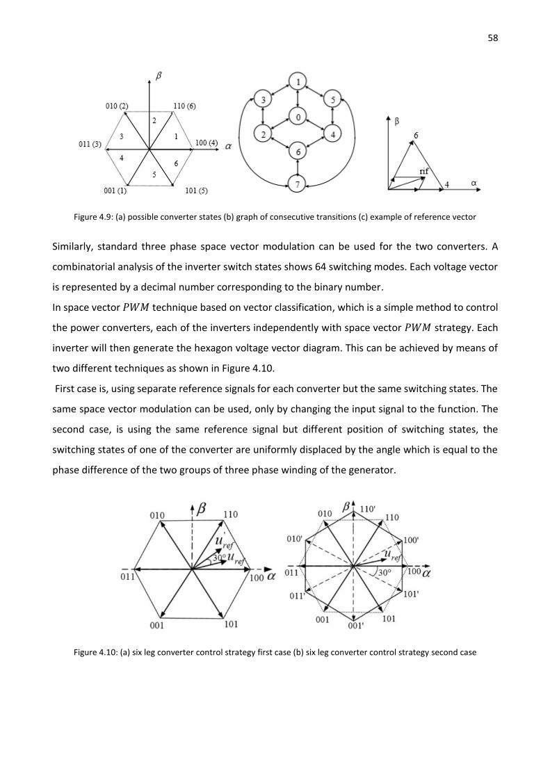
58

Figure 4.9: (a) possible converter states (b) graph of consecutive transitions (c) example of reference vector

Similarly, standard three phase space vector modulation can be used for the two converters. A

combinatorial analysis of the inverter switch states shows 64 switching modes. Each voltage vector

is represented by a decimal number corresponding to the binary number.

In space vector 𝑃𝑊𝑀 technique based on vector classification, which is a simple method to control

the power converters, each of the inverters independently with space vector 𝑃𝑊𝑀 strategy. Each

inverter will then generate the hexagon voltage vector diagram. This can be achieved by means of

two different techniques as shown in Figure 4.10.

First case is, using separate reference signals for each converter but the same switching states. The

same space vector modulation can be used, only by changing the input signal to the function. The

second case, is using the same reference signal but different position of switching states, the

switching states of one of the converter are uniformly displaced by the angle which is equal to the

phase difference of the two groups of three phase winding of the generator.

Figure 4.10: (a) six leg converter control strategy first case (b) six leg converter control strategy second case

59

Despite the fact that for this modulation technique only the (𝛼 − 𝛽) subspace is controlled, the

current harmonics from the phase currents spectra are considerably reduced compared with the

conventional 𝑆𝑉𝑀.

In fact, in both methods, the harmonic currents such as 5𝑡ℎ, 7𝑡ℎ, and 17𝑡ℎ, etc. are inherently

eliminated without extensive computations. The vector classification is simpler than the vector

space decomposition technique from the point of view of implementation complexity, because the

switching state vectors are mapped into the inverter basis frame rather than the machine basis

frame. And the maximum modulation index increases by 3.59% compared to vector decomposition

technique. Consequently, the vector classification techniques can be easily implemented with low

cost fixed-point 𝐷𝑆𝑃 controllers.

Figure 4.11: vector classification technique

61

Chapter 5

Simulations

n the last chapter simulation results are presented. It will be firstly introduced the machine

from which the data were taken, then the various blocks implemented in 𝑀𝑎𝑡𝑙𝑎𝑏/

𝑆𝐼𝑀𝑈𝐿𝐼𝑁𝐾. PID tuning procedure is explained along with motor mode operation. In the

end, generator mode operation will be largely illustrated, explaining obtained results and how

it was possible to conciliate 𝑆𝐼𝑀𝑈𝐿𝐼𝑁𝐾 signal logic with 𝑆𝑖𝑚𝑃𝑜𝑤𝑒𝑟𝑆𝑦𝑠𝑡𝑒𝑚 circuit logic in order

to simulate efficiently power electronic and power system components.

5.1 Machine data

Before the presentation of the simulations in 𝑀𝑎𝑡𝑙𝑎𝑏/𝑆𝐼𝑀𝑈𝐿𝐼𝑁𝐾 it is better to describe the

machine that was taken as reference in the work. In Table 5 are shown the most important

parameters from which the others can be derived.

Table 5: machine data

I

62

5.2 Machine model

The first step was to write in 𝑀𝑎𝑡𝑙𝑎𝑏/𝑆𝐼𝑀𝑈𝐿𝐼𝑁𝐾 the machine model starting from the derived

machine equations. As it was explained in rotating 𝑑 − 𝑞 reference frame it is easy to control the

machine because the torque depends just on the current component 𝑖𝑞1, due to the particular

transformation that was done on machine variables.




𝑣𝑞1




𝑣𝑑2



𝑖𝑞2




(3.28)

To use it, it is necessary to make the integral of the current’s derivatives in order to make

𝑆𝐼𝑀𝑈𝐿𝐼𝑁𝐾 solve the system of equations. The machine system is shown below in Figure 5.1 in

which the different terms shown in the equations are highlighted.

Figure 5.1 machine equations in 𝑀𝑎𝑡𝑙𝑎𝑏/𝑆𝐼𝑀𝑈𝐿𝐼𝑁𝐾

63

Figure 5.2 electromotive force contributes

As can be seen the contributes due to back electromotive forces are treated as disturbances, this is

because the only terms able to change the current (absorbed or delivered) are the voltages:

𝑢𝑑1= 𝑅𝑠𝑖𝑑1

+ 𝑝𝐿𝑑1𝑖𝑑1

𝑢𝑞1

= 𝑅𝑠𝑖𝑞1+ 𝑝𝐿𝑞1

𝑖𝑞1

𝑢𝑑2

= 𝑅𝑠𝑖𝑑2+ 𝑝𝐿𝑑2

𝑖𝑑2

𝑢𝑞2

= 𝑅𝑠𝑖𝑞2+ 𝑝𝐿𝑞2

𝑖𝑞2

(5.1)

In fact, writing the equations in the Laplace’s domain the transfer function (𝑇𝐹) of the input voltage

(without considering disturbances) and the output current can be obtained:

𝐼𝑑1(𝑠) =

1

𝑅𝑠+𝑠𝐿𝑑1

𝑈𝑑1(𝑠) 𝐼𝑞1

(𝑠) =1

𝑅𝑠+𝑠𝐿𝑞1

𝑈𝑞1(𝑠)

𝐼𝑑2(𝑠) =

1

𝑅𝑠+𝑠𝐿𝑑2

𝑈𝑑2(𝑠) 𝐼𝑞2

(𝑠) =1

𝑅𝑠+𝑠𝐿𝑞2

𝑈𝑞2(𝑠)

(5.2)

64

5.3 Torque expression

The electromagnetic torque expression was written considering equation 3.34 which is:

𝑇𝑒 = 𝑛𝑝Ψ𝑑1

∗ 𝑖𝑞1= 𝑛𝑝[Ψ𝑃𝑀,𝑑1

𝑖𝑞1+ 𝑖𝑞1

𝑖𝑑1(𝐿𝑑1

− 𝐿𝑞1)]

(3.34)

The model in 𝑀𝑎𝑡𝑙𝑎𝑏/𝑆𝐼𝑀𝑈𝐿𝐼𝑁𝐾 is shown in Figure 5.3:

Figure 5.3 torque expression

5.4 PI regulator tuning

Once found the 𝑇𝐹𝑠, the next step was to find current and speed regulators parameters. In this

work 𝑃𝐼 regulators were used and they were tuned using the 𝑀𝑎𝑡𝑙𝑎𝑏 application: 𝑇𝑢𝑛𝑒𝑟.

5.4.1 Current regulator

As we said the currents (and so the torque) are controlled by the 𝑢 voltages, the Figure 5.4 shows

the scheme of a current regulator, in particular in this scheme it was considered that:

Disturbances are compensated or not present

The modulator is a unity gain

For a better representation of the power supply, the unity gain could be replaced with a delay whose

value is tied to the switching time of the converter switches. If the modulator is based on a 𝑃𝑊𝑀

technique, for example, the delay between the instant of the reference variation and its

implementation varies from 0 to the entire period of switching. On average, we can assume a delay

equal to one half the switching time.

65

Figure 5.4: Procedure to find 𝐾𝑝 , 𝐾𝑖 gains

The scheme in Figure 5.4 is representative of just one winding set. Due to the presence of second

winding set it was necessary to do the procedure for both sets.

The procedure used to find 𝐾𝑝 , 𝐾𝑖 of the regulator (for example for the 𝑞1 axis) was:

Insert the transfer function in 𝑀𝑎𝑡𝑙𝑎𝑏:

Then the equation was open in 𝑃𝐼𝐷 𝑇𝑢𝑛𝑒𝑟, which allows to choose bandwidth and phase

margin of the output in the frequency domain. Additionally, time domain response can be

tuned as well in order to obtain a more robust and/or faster response. Below, the example

of the application is presented, in which time domain and frequency domain responses are

considered in order to find the optimal value of the two parameters.

Figure 5.5 time domain response function of 𝑃𝐼 parameters

66

Figure 5.6 frequency domain response function of 𝑃𝐼 parameters

The 𝑃𝐼 parameters were chosen as a tradeoff between a correct and fast response and the

maximum allowed value of the parameters themselves, in particular it is empirically known that the

𝐾𝑖 cannot overcome the value 10000.

In the work the value of the 𝐾𝑖 parameters was maintained around 5000.

The same was done for the other machine fictitious axis, in this way the regulator were tuned

for both type of operation: motor and generator in order to obtain a good steady state and

transient response, moreover the system has a good response to external disturbances

5.4.2 Speed regulator design

As it was said the main focus of the work was the use of the machine as generator but, in order to

verify the correctness of both the machine model and the regulator tuning process, the simulation

was tested as machine operates as motor. To do so, it was necessary to design also the speed

regulation loop and insert the mechanical equation, as shown in Figure 5.7.

Figure 5.7 speed loop design scheme

67

The transfer function 𝐹𝑖(𝑠) corresponds to the presented current loop. During the tuning process

of speed regulator, inner loop transfer function can be considered as a unity gain because the

bandwidth of the current loop is near to 1000 𝑟𝑎𝑑 𝑠⁄ (a decade bigger than the current loop one).

Figure 5.8 transfer function and sensitivity function

This is possible because the bandwidth of the speed loop transfer function is confined in the zone

in which the transfer function 𝐹(𝑗𝜔) has a gain equal to 1. The function 𝐹(𝑗𝜔) is the sensitivity

transfer function of the loop and represents the transfer function between the output variable and

the reference value of the input variable. The possibility of considering the current loop 𝑇𝐹 equal

to 1 is a good advantage because the regulation becomes easier, this method is called frequency

decoupling.

5.5 Mechanical load equation

For motor machine operation the mechanical equation related to the load was written as well:

𝜔𝑒 =

𝑛

𝐵𝑣 + 𝑠𝐽 (𝑇𝑒 − 𝑇𝑚)

(5.3)

Once obtained the electromagnetic torque, (see Figure 5.9) and subtracting the load torque (which

is a disturbance) the rotational speed (in 𝑒𝑙. 𝑟𝑎𝑑/𝑠) can be obtained through the transfer function

associated with the rotational masses: load + electrical motor. The two parameters are the inertia

( 𝐽 ) of the two masses and the viscous friction coefficient (𝐵𝑣) , the chosen values for these two

quantities are:

𝐽 = 0.065 𝐾𝑔 𝑚2

𝐵𝑣 = 0.21 𝑁𝑚 𝑠

68

Figure 5.9 mechanical load equation

5.6 Park’s transformations

The last blocks needed are the Park’s transformations blocks. As it was said they transform the phase

variable in Park component variables through a transformation. To obtain the transformation, the

matrix 𝑻3(𝜃) presented in Chapter 3 was implemented in 𝑀𝑎𝑡𝑙𝑎𝑏/𝑆𝐼𝑀𝑈𝐿𝐼𝑁𝐾 and shown in Figure

5.10. The inverse transformation 𝑻3−1(𝜃) is obtained by transposition of matrix 3.25.

𝑻3(𝜃) = (𝑻𝑝(𝜃 + α) 𝑻𝑝(𝜃 − α)

𝑻𝑝 (𝜃 + α +𝜋

2) 𝑻𝑝 (𝜃 − α −

𝜋

2))

(3.25)

It is important to notice that since this is the transformation in a rotating frame it takes as an input

the rotational speed 𝜔𝑒 and then through integration the 𝜃𝑒(𝑡) value of the rotational position is

obtained. The 𝑓(𝑢) functions are the actual equations which transform the time variables in Park’s

variables while the factor 1√3

⁄ is needed to achieve power invariance.

Figure 5.10 Park’s transformation

69

5.7 Motor mode operation

5.7.1 System configuration

The equations and blocks needed are already presented, consequently it is possible to show the

obtained results in the case of motor operation. As it was said, it was necessary to perform some

simulations in order to verify if the control system worked correctly and if the machine had a

behavior similar to the one taken as reference. The modulator wasn’t taken in exam because it was

not important for the purpose of the first simulations.

Input variables were:

The rated electrical speed, 𝜔𝑒 which is 𝜔𝑒_𝑛𝑜𝑚 = 𝑛𝑝𝜔𝑚_𝑛𝑜𝑚 ,where the nominal speed was

given (350 𝑟𝑝𝑚) and the number of poles (𝑝) was given as well, and

The rated resistant torque, which means that to obtain a steady state situation the motor

must generates an equal and opposite torque, which is in turns the nominal one obtained

through calculations.

In particular, the nominal torque value was obtained knowing that:

𝑃𝑒𝑙_𝑛𝑜𝑚 = √3 𝐸𝐿2𝐿𝐼𝑛𝑜𝑚 = 14146𝑊 (5.4)

From which can obtained the output mechanical power:

𝜂 =

𝑃𝑒𝑙_𝑛𝑜𝑚 − 3𝑅𝑠𝐼𝑛𝑜𝑚2

𝑃𝑒𝑙_𝑛𝑜𝑚= 0.943

(5.5)

Just Joule losses in stator windings were considered in the efficiency computation. Knowing the 𝜂

can be write:

𝑃𝑚_𝑛𝑜𝑚 = 𝜂𝑃𝑒𝑙_𝑛𝑜𝑚 = 13339𝑊 (5.6)

And, knowing that:

𝑃𝑚_𝑛𝑜𝑚 = 𝑇𝑚_𝑛𝑜𝑚 𝜔𝑚_𝑛𝑜𝑚 (5.7)

The nominal torque is obtained:

70

𝑇𝑚_𝑛𝑜𝑚 =

𝑃𝑚_𝑛𝑜𝑚

𝜔𝑚_𝑛𝑜𝑚= 364.5𝑁𝑚

(5.8)

Considering this result we can also obtain the nominal 𝑖𝑞1_𝑛𝑜𝑚 able to generate the nominal torque:

𝑖𝑞1_𝑛𝑜𝑚

=𝑇𝑚_𝑛𝑜𝑚

𝑛𝑝 Ψ𝑃𝑀= 63.75 𝐴

(5.9)

Where:

Ψ𝑃𝑀 =

𝐸𝐿2𝐿_𝑛𝑜𝑚

√3⁄

𝑛𝑝 𝜔𝑚_𝑛𝑜𝑚= 1.4295 𝑊𝑏

(5.10)

Ψ𝑃𝑀 is the flux of the permanent magnets chosen for the machine and it is chosen as a compromise

between high performances and low manufacture’s costs. In this case, it can be observed that the

machine rotor was made by 𝐼𝑃𝑀𝑠, this is the reason why the torque expression presented in

equation 3.34 has two contributes: anisotropy torque and excitation torque contribution. But

considering the current 𝑖𝑑1= 0 actually we treat the machine like an isotropic machine, in which

we consider just the excitation torque component. This is done because interior permanent

magnets are less expensive and easier to be realized with respect to surface permanent magnets,

consequently this solution has been chosen. Then anisotropy torque component is made inefficient

because it makes the control system more difficult; this operation, however does not affect too

much the performances of the machine.

Figure 5.11: complete simulated model

71

5.7.1 Simulation results

As it is shown in Figure 5.12 The electromagnetic torque (𝑇𝑒 , in green) follows very closely the

mechanical resistance torque (𝑇𝑚 , in black dashed line) the mechanical torque reference was given

as a step from time 0𝑠 to time 4𝑠, the insertion of the load was gradual to avoid high transient

variations. Now, it is interesting to understand if with the nominal generated electromagnetic

torque, the other quantities are as expected and if the control system works correctly.

For example, in Figure 5.13 the electrical angular speed (𝑒𝑙. 𝑟𝑎𝑑 𝑠⁄ ) is shown. The reference speed

at which the machine should rotate is the nominal one.

Figure 5.12: mechanical vs electromagnetic torque

Figure 5.13: reference vs actual speed

It can be seen that the control system works correctly, after 4𝑠 when the resistant torque remains

constant, the rotational speed of the machine follows the speed reference value. This result is

possible only if the current (𝑞1 axis) controller works efficiently as well. Figure 5.14 shows the

72

correctness of the most important current component (𝑖𝑞1) , because as it was said the dynamic of

the machine only depends on the value of this current.


The current (in green) follows very closely the reference value (black), reference value which is the

output of the speed controller in the first stage. Another important point to highlight is the current

value at steady state, which is 65 𝐴, very near to the one we expected to find. This difference will

bring to other differences in phase currents and in absorbed electrical power with respect to

nominal values, due to dissipations that probably are not given in nominal data. Anyway the

difference is not too high and the studied model can be considered reliable.

The correctness of the other three current controllers are verified and shown in the following

figures.


73



The control works correctly and the illustrated model can be considered a good solution to

schematize the machine behavior. In the second winding set it can be seen that there are not

transient phenomena, this is right since the two currents (𝑖𝑑2 , 𝑖𝑞2

) are both taken with a reference

value equal to 0 and as expected they are not affected on what happens in the other winding set,

due to decoupling. Instead as regards current 𝑖𝑑1 it can be highlight that the presence of the

motional term (disturbance) in the current equation affects its time variation. Anyway the effect of

the disturbance is small and so the controllers are working correctly. The parameters of the 𝑃𝐼𝑠

found in this test are the ones used later in the generator mode of operation.

The last important quantities to be checked are the phase currents, obtained anti-transforming the

𝑑 − 𝑞 currents absorbed by the fictitious machine and caused by the reference voltages obtained

through the controllers, and the power: mechanical output power and electrical absorbed power.

As for the current using the anti-transform block the following results were obtained (Figure 5.18),

all the six phase currents are presented in the same plot to highlight the phase shift between

currents of the same winding set and currents of different winding sets.

74

The first winding set currents (in blue) are shifted by 30 𝑑𝑒𝑔 with respect to currents of the second

winding set. This result was expected, in fact, the windings are space displaced by 30 𝑒𝑙. 𝑑𝑒𝑔 which

means that the magnetic flux generated by the 𝑃𝑀𝑠 invests each coil of different winding sets after

30 𝑒𝑙. 𝑑𝑒𝑔. In the following plots, for clarity purposes, just the first winding set currents are shown.

Figure 5.18: phase currents of the two winding sets

The maximum value of the absorbed currents was expected too, in fact considering that the only

current component taken different from 0 was the 𝑞1 component, using the 𝑻3(𝜃) it is obtained

that:

[ 𝑖𝑎1

𝑖𝑏1

𝑖𝑐1

𝑖𝑎2

𝑖𝑏2

𝑖𝑐2]

= 𝑻3(𝜃) [

0𝑖𝑞1

00

]

(5.11)

And knowing that the matrix 𝑻3(𝜃) introduces a coefficient 1√3

⁄ it can be write (for the modulus

of a generic phase current, in the example was taken current 𝑖𝑎1):

𝑖𝑎1_𝑚𝑎𝑥

=𝑖𝑞1

√3⁄ = 37.5 𝐴 (5.12)

Which corresponds to a 𝑟𝑚𝑠 value of:

75

𝑖𝑎1_𝑟𝑚𝑠

=𝑖𝑎1_𝑚𝑎𝑥

√2⁄ = 26.5 𝐴 (5.13)

Which is a value very close to the nominal one, the slight difference is due to the problem that was

already explained.

As concerns the power it was necessary to implement in 𝑀𝑎𝑡𝑙𝑎𝑏/𝑆𝐼𝑀𝑈𝐿𝐼𝑁𝐾 two different

relations, the first for the input electrical power, which is:

𝑃(𝑡) = 𝑣𝑑1𝑖𝑑1


+ 𝑣𝑑2𝑖𝑑2


(3.)

In which it is doubtless that the main contribute if not the only one is given by the term 𝑣𝑞1𝑖𝑞1

, in

fact as it was observed the other currents are equal to 0 or different to 0 just in the initial transient

part.


Due to stator resistance, efficiency of the simulated machine is not 1, but it should be considered

also that mechanical losses are here neglected. Even though they are not so large it is better to

consider them in order to explain in a better way the real behavior of the machine. The steady state

value considered as nominal was 15886 𝑊.

The second power relation, the one which provides the mechanical output power is:

𝑃𝑚 = 𝑇𝑚𝜔𝑚 = 𝑇𝑒𝜔𝑒

𝑛𝑝⁄

(5.14)

76

Which gives, after the transient, a mechanical output power of 13641𝑊.

To conclude it can be said that the model is quite accurate and the control system works correctly

for the simulated cases which were considered. Now, it will be presented the main important case

which is the generator operation.

5.8 Generator mode operation (modulator as unity gain)


In generator operation the machine model was maintained identical to the previous case, changing

the control structure and the input variables. In particular, in this operation mode, the electrical

speed is decided by the prime mover, which is the wind turbine. It was imagined a system in which

turbine blades were directly connected to the machine. The speed at which it rotates is decided

from the turbine control system in order to extract the maximum wind power (as it was seen in

Chapter 4). This part of the control system was neglected and it was considered that the speed

which drives the two rotational masses (wind turbine blades and electrical generator) was the one

which guarantees the maximum extracted power. The chosen speed was a ramp and it is shown in

Figure 5.20, the rotational speed is increased from 0𝑠 to 4𝑠, to avoid sudden stresses.


The input variable was the electromagnetic torque, in the simulation the nominal one was taken in

order to show the maximum extractable power from the wind turbine (if blades rotates at their

nominal speed) but in real systems in which the electrical delivered power has to be controlled, the

torque and the power vary considering the equation:

77

𝑃𝑚 = 𝑇𝑚 𝜔𝑚 ≅ 𝑃𝑒𝑙 (5.14)

In which the speed hasn’t to be considered as a constant, in the evidence of what it was said before,

i.e. the necessity to maintain 𝑐𝑝 as high as possible with different wind speed situations.

Figure: 5.21: generator simulation without modulator


Obtained results are shown, the main purpose is to verify if the machine and control system work

correctly in nominal operation conditions. To do so, modulator is not taken into account, meaning

that the six leg inverter is considered as ideal (as like unity gains).

The chosen torque was 𝑇𝑒𝑙_𝑛𝑜𝑚 = −364.5 𝑁𝑚, the torque increased after the speed reached its

nominal value, this operation allows better performances of the control system and it was used also

for the other simulation tests. The minus sign stands for the fact that with our signs conventions,

electrical and mechanical power were taken as they were entering the system. In this way the

electrical power was an outgoing power. Choosing the torque, means, in turn, choosing the voltages

at machine terminals able to deliver the correct current and so generate the desired resistant

electromagnetic torque. This will be shown in a better way when the modulator will be introduced.

As for now, considering again that the reference values of currents 𝑖𝑑1 , 𝑖𝑑2

, 𝑖𝑞2 are taken equal to

zero, the following results are shown:

78


As it can be seen the actual electromagnetic torque follows very well the reference value of the

resistant electromagnetic torque. As it was largely said, since the electromagnetic torque depends

on current 𝑖𝑞1 means that also that current has to follow its reference, which is obtained through

the equation:

𝑖𝑞1_𝑟𝑒𝑓 =

𝑇𝑒𝑙_𝑟𝑒𝑓

𝑛𝑝 𝜙𝑃𝑀

(5.9)

In fact, its dynamical behavior is:


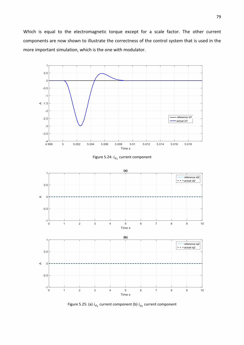
79

Which is equal to the electromagnetic torque except for a scale factor. The other current

components are now shown to illustrate the correctness of the control system that is used in the

more important simulation, which is the one with modulator.


Figure 5.25: (a) 𝑖𝑑2 current component (b) 𝑖𝑞2

current component

80

For the current components 𝑖𝑑2 , 𝑖𝑞2

the same comments made for motor mode operation are still

valid. As concerns phase currents, it can be stated that imposing a nominal torque means to impose

the nominal 𝑟𝑚𝑠 current at the output of the machine. As it will be shown in the next simulation

test, in the real machine this is achieved acting on power converter’s switches which are the

electrical device able to control the terminal voltages of the machine and, consequently, they

control the phase currents. The phase currents of the first winding set are shown in the figure below,

which is Figure 5.26.


The results in Figure 5.26 were explained in the previous paragraph as regards motor mode

operation. It can be interesting to note that in this operation mode the current is delivered instead

of being absorbed.

81

5.9 Generator mode operation (complete model)


The studied configuration is the one presented in Figure 5.28, in which the double star synchronous

generator (coaxial with the wind turbine) is connected to the 𝐷𝐶 link through a six leg converter. It

is considered that the grid side bus is an infinite bus, with the meaning that, this bus imposes the

voltage and the frequency at its terminal.

Figure 5.28: studied configuration system

In turns, have an infinite bus at the grid terminals means that the voltage at the 𝐷𝐶 bus is imposed

by the grid, the only quantity which can be controlled is the current injected. (and so the active

power) It also means that the six leg inverter behaves as if it was supplied with a 𝐷𝐶 voltage 𝑉𝐷𝐶 .

Controlling the inverter switches, the machine terminal voltages are controlled and so the amount

of current allowed to circulate and injected in the grid. In this configuration it is possible to work

with unity power factor.

Figure 5.29: single leg converter operation

82

Under Rectifier mode operation, the converter works like Boost converter. The upper switch and

lower diode work complementarily, the blue line shows the direction of current flow. Under Inverter

mode of operation, the converter works like Buck converter. The lower switch and the upper switch

and lower diode work complementarily which is shown by red line in Figure 5.29. The relationship

between input voltage (assumed sinusoidal) and converter voltage, ignoring the harmonics, can be

easily shown by a phasor. From Figure 5.30, the converter voltage is higher that the input voltage in

both modes near unity power factor operation. Therefore, the 𝐷𝐶 link voltage should be sufficiently

larger than diode rectification voltage otherwise the converter will behave like common diode

bridge.

Figure 5.30: (a) rectifier mode operation (b) inverter mode operation

Both in unity power factor operation

5.9.2 Description of the simulation

The modulator is here added to the simulation in order to illustrate in which way the real system

would work. To do so, the signal logic has to be synchronized with the circuit logic introduced by

𝑆𝑖𝑚𝑃𝑜𝑤𝑒𝑟𝑆𝑦𝑠𝑡𝑒𝑚𝑠. The 𝑆𝑖𝑚𝑃𝑜𝑤𝑒𝑟𝑆𝑦𝑠𝑡𝑒𝑚𝑠’ library is needed because it allows to introduce

electrical components, such as: resistances, inductors, capacitances, inverters, generators, and so

on.

In particular, the inverter and the control system of the inverter itself has been added. The system

becomes like the one shown in Figure 5.31 for motor mode operation. It is important is to note that

now there is not a direct passage from the control system to the machine terminals but instead, the

control system gives the reference values needed to generate the gate signals, which through the

inverter can control the terminal voltages and consequently, the currents.

83


Let us consider now in more detail how the system works.

Starting from the control system illustrated in Figure 5.32, the reference value of the output currents

are selected, except for 𝑞1 axes in which the resistant electromagnetic torque, which is, as it was

said before a scaled value of the 𝑞1current component.

Figure 5.32: control system

In the real system, these voltages must be modulated by the inverter. To do so, the inverter receives

the gate signals from the two 𝑃𝑊𝑀 generators. The process is shown in Figure 5.33, the reference

voltages, obtained from the regulation system are anti-transformed through anti-transform Park’s

block, then the signals are modified (scaled to obtain a per unit signal) in order to be compared with

the triangular waveform inside the block 𝑃𝑊𝑀 generator, and so generate the gate signals which

control opening and closing of the switches inside the inverter legs.

84

Figure 5.33: gate signal generators

In this way, gate control signals 𝑔1 and 𝑔2 are obtained and sent to the six leg inverter which is

already inside the circuit logic domain.

5.9.3 Six leg converter

The inverter receives the gate control signals 𝑔1 and 𝑔2. In this way, the inverter legs, generate the

desired voltages at the machine terminals. These phase voltages are measured through the

voltmeters and sent to the machine terminals using the block 𝑔𝑜 𝑡𝑜 (blue, in Figure 5.34)

Figure 5.34: inverter and 𝐷𝐶 link model

As it was said, the measured voltages are sent to the machine model, as shown in Figure 5.35, with

the meaning that: with that specific combination of open and closed switches the delivered amount

85

of current is the one obtained through the mathematical model of the machine (i.e. solving the

differential equations of the machine). Before introducing the voltages in the machine model they

have to be transformed using the Park’s transformation block.


The obtained currents are the input of the controlled generators Figure 5.34 (in yellow), they are

current generators current controlled. The control signals which drive the generators are in the

signal domain (𝑆𝐼𝑀𝑈𝐿𝐼𝑁𝐾) while the generators themselves are in the circuit domain

(𝑆𝑖𝑚𝑃𝑜𝑤𝑒𝑟𝑆𝑦𝑠𝑡𝑒𝑚). In this way, the two logics can be easily synchronized and advantages of their

combined use can be exploited.


The results are shown, in which as before, the aim is to understand the correct behavior of the

machine and control system. It was already proved the correctness of the machine model and the

good behavior of the control system in the case in which the modulator was considered as unity

gain. Now, it is important to understand if the complete system works correctly and if possibly the

control system can be used with a real machine and a real six leg inverter. The input electromagnetic

torque is a ramp with maximum value equal to 𝑇𝑒𝑛𝑜𝑚= −364.5 𝑁𝑚.

86


In Figure 5.36 the imposed rotational speed is shown. With respect to the previous case the ramp

was increased, it reached the nominal speed after 0.1𝑠, it was done to decrease the simulation time,

the change does not affect the correctness of the simulation or the performances of the control

system.

following the same steps used for the previous case, the first plot shows the time variation of the

electromagnetic torque.


It can be seen that follows very closely its reference value. The next is the 𝑖𝑞1 current component,

shown in Figure 5.38:

87


And the other current components are:

Figure 5.39: 𝑖𝑑1

current component

Figure 5.40: 𝑖𝑑2

current component

88

Figure 5.41: 𝑖𝑞2

current component

The control system works correctly, the amplitude of the oscillations around the reference value are

very low although they are present. Dynamical stresses in transient operation are not too high and

the 𝑃𝐼𝑠 regulation is fast. It can be said that if this control system would be applied to a real machine

and inverter, it would give good results in terms of performances.

However, it is important to show the behavior of the phase currents, which are the actual circulating

current components, their time evolution is presented in Figure 5.42, for the first winding set.


These are the currents delivered by the machine, so the currents at the machine terminals. They are

generated by the inverter which modulates the voltages, the next plots show these voltages, they

are shown for the first winding set.

89

Figure 5.43: actual phase voltages (first winding set)

As it was already said in Chapter 4, 𝑃𝑊𝑀 modulate the voltages in this way. Important to note is

the magnitude and frequency of the first harmonic along with magnitude and frequency position of

the other harmonics. Neglecting for now the issues related to higher order harmonics (which are

not the main focus of the work) let us consider the first harmonic of the voltage 𝑣𝑎1(The black line

in Figure 5.43 ).

Figure 5.44: first harmonic of 𝑣𝑎1

For the sake of clarity was shown just a part of a period. The other phase voltages have the same

time behavior as 𝑣𝑎1 with a phase displacement due to winding position. To complete the set of the

machine terminal’s quantities, phase current, phase voltage of phase 𝑎1 and line to line voltage are

shown together in the same plot (Just the first harmonic is presented).

90

Figure 5.45: 𝐴𝐶 variables

Obviously 𝑣𝑎𝑏1 was found as: 𝑣𝑎𝑏1

= 𝑣𝑎1− 𝑣𝑏1

and in fact its modulus is √3 times the modulus of

𝑣𝑎1. Another important data to take into account is the phase displacement between 𝑣𝑎1

and 𝑖𝑎1. It

is desirable to have 𝑐𝑜𝑠𝜑 = 1.

From the figure can be seen that:

∆𝑡 = 𝑡2 − 𝑡1 = 0.005𝑠

(5.15)

Where

𝑡2: time instant of the current peak

𝑡1: time instant of the voltage peak

So, knowing that:

𝜔𝑒∆𝑡 = 𝜑 = 0.733

(5.16)

It can be proved that the 𝑐𝑜𝑠𝜑 is equal to 1. Precisely its value is 0.999.

The last important quantities remained to be shown are the 𝐷𝐶 ones. In particular, the most

important is the delivered 𝐷𝐶 power which is the one injected into the grid. This power was

computed as:

𝑃𝐷𝐶 = 𝑉𝐷𝐶𝐼𝐷𝐶

(5.17)

91

Where 𝑉𝐷𝐶 , as it was said before is fixed by the infinite bus and its value was taken equal to 750𝑉.

Instead, in Figure 5.46 the direct current 𝐼𝐷𝐶 and its mean value are shown.

Figure 5.46: 𝐷𝐶 side current

Taking the mean value of the current 𝐼𝐷𝐶, the last Figure shows the two compared powers:

mechanical input power and electrical output power.

Figure 5.47: mechanical vs electrical power

92

5.10 Generator mode operation with uncontrolled diode bridge


To reduce the number of power converters, the idea was to substitute one of the two machine side

converters with a diode bridge, as shown in Figure 5.48a. The three phase diode bridge has the

advantage of being less expensive but it makes impossible to control the electrical quantities of the

second winding set. The simulation was carry out to study the behavior of the system in this

particular configuration and to understand if it was possible to find a way to mitigate the problems

derived by the insertion of an uncontrolled component such as the diode bridge.

Figure 5.48: (a) electrical circuit model (b) DC bus voltage regulation

5.10.2 DC bus voltage regulation

To take into account the insertion of an uncontrolled element it was necessary a more detailed

model of the grid converter: the 𝐷𝐶 voltage source was substituted by a controlled current source

and a capacitance. The 𝐷𝐶 control system was tested using last system configuration, which is the

one with both controlled power converters.

The control signal of the current source (𝐼𝑟𝑒𝑓) was decided by the control system. Figure 5.48b shows

the voltage control loop and the generation of the correct 𝐼𝑐 reference value able to maintain the

voltage as constant as possible on its reference value. The capacitance was 𝐶 = 100 𝑚𝐹 and it was

charged at 750𝑉. Then, the capacitance current 𝐼𝑐 is compared with the machine output current

(𝐼𝑚𝑎𝑐ℎ𝑖𝑛𝑒), as shown in Figure 5.49b (the signs are arbitrary but they need to be chosen correctly).

The machine current delivered by the machine was decided through power considerations

explained in Chapter 4.

𝑃𝑚 = 𝑇𝑒𝜔𝑚 ≅ 𝑉𝐷𝐶𝐼𝑚𝑎𝑐ℎ𝑖𝑛𝑒 = 𝑃𝐷𝐶 (5.18)

93

Figure 5.49: (a) mechanical power (b) 𝐼𝑟𝑒𝑓 selection

It wasn’t taken into account mechanical or electrical losses, this fact allows to find an easy

expression for the 𝐷𝐶 output current. From equation 5.18 the machine current can be obtained:

𝐼𝑚𝑎𝑐ℎ𝑖𝑛𝑒 =

𝑇𝑒𝜔𝑚

𝑉𝐷𝐶

(5.19)

As it was said, 𝐼𝑚𝑎𝑐ℎ𝑖𝑛𝑒 is compared with the 𝐼𝑐 and the signal sent to the modulator (which is here

considered as ideal). The grid side power converter allowed the correct 𝐼𝑟𝑒𝑓 to circulate (taking into

account the machine current 𝐼𝑚𝑎𝑐ℎ𝑖𝑛𝑒 ) in order to let 𝐼𝑐 through the capacitor. The 𝐷𝐶 bus voltage

was controlled and it follows its reference in all machine operation conditions, it can be said that

the voltage control worked correctly, as shown in Figure 5.50.

Figure 5.50: regulated 𝐷𝐶 voltage

The system was completely decoupled, grid side variables can be considered independent from the

machine side variables.

94

5.10.3 Simulation

The system configuration shown in Figure 5.48a brought into light difficulties in the prediction of

the machine behavior along with different cases in which the diode bridge didn’t work correctly.

This situation was anyway expected because, in order to be able to work, power converter needs a

𝐷𝐶 bus voltage greater or equal than √2 𝑉, which is the maximum value of the machine voltage

waveform. While, the diode bridge needs the 𝐷𝐶 bus voltage below that value, otherwise diode is

not able to conduct. It was decided to consider another system configuration. The two winding sets

were divided and connected to two different voltage sources (the 𝐷𝐶 regulation wasn’t taken into

account for this purpose). The second winding set 𝐷𝐶 bus voltage was set at 150𝑉. With this

particular system configuration the following results were obtained:

The reference torque was equal to −100 𝑁𝑚, this value was chosen to avoid overload of

one of the two machine stars. The actual electromagnetic torque followed the fixed

reference value, as shown in Figure 5.51.

Figure 5.51: electromagnetic torque (with uncontrolled diode bridge)

The obtained result for the electromagnetic torque is a consequence of a correct work of the

control system on the fictitious current components: 𝑖𝑑1 and 𝑖𝑞1

. In fact, thankfully, the

control system succeeded in the current regulation. The results obtained for the torque and

these two current components are good starting point for the creation of a newer and more

performing control system. In Figures 5.52 and 5.53 𝑖𝑑1 and 𝑖𝑞1

are shown.

95

Figure 5.52: 𝑖𝑑1 current component (uncontrolled bridge)

Figure 5.53: 𝑖𝑞1 current component (uncontrolled bridge)

As it was expected current components 𝑖𝑑2 and 𝑖𝑞2

were out of control but they never exceed

dangerous values and achieved the steady state their value was constant.

Last important quantities to show are the absorbed mechanical power and delivered 𝐷𝐶

electrical powers.

Figure 5.54: mechanical and electrical powers (uncontrolled bridge)

The obtained results were expected and not so terrible but in the end the system didn’t work in

acceptable way. This is why it was necessary to find a better way to control the system.

96

5.10.4 Innovative control set up

As already said, the two power electronic components cannot work with the same 𝐷𝐶 bus voltage

level. Additionally, Figure 5.54 shown that without an appropriate control strategy it is impossible

to achieve good performances of the system. In fact, with those initial data the diode bridge

delivered most of the output power, while the power converter carried a very low share of the total

power. A solution was found using the configuration set up shown in Figure 5.55a, in which 𝐷𝐶

buses were maintained separated but just the one connected to the diode bridge was controlled.

The other three phase set is thought to be in steady state.

Figure 5.55: (a) system configuration (b) 𝐷𝐶 bus regulation

The current controlled current source, as before, represents the grid side power converter

(modulator wasn’t taken into account). The idea is to use the grid power converter to regulate the

diode bridge delivered current acting on the 𝐷𝐶 bus voltage level. This can be achieved

because 𝑃𝐷𝐶 = 𝑉𝐷𝐶𝐼𝐷𝐶. As soon as the delivered power can be considered constant, voltage and

current are inversely proportional, thus varying 𝑉𝐷𝐶, it is possible to regulate the delivered current.

Figure 5.56: corrective term control system

97

The result, however, is a not perfectly constant value of the 𝐷𝐶 bus voltage 𝑉𝐷𝐶 2. Using this control

strategy the most important part is the choice of the correction term, in Chapters 4 and 5 was

explained that wind turbine system cannot always deliver the nominal power due to varying wind

speed or grid requirements. So, the reference 𝐷𝐶 current value for the bridge connected three

phase winding was chosen in an easy way: it was half the current demanded to the controlled

winding set, which is:

𝐼𝑚𝑎𝑐ℎ𝑖𝑛𝑒_𝑟𝑒𝑓 =𝑃𝑚

2 𝑉𝐷𝐶1

=𝑇𝑒 𝜔𝑚

2 𝑉𝐷𝐶1

In this way, it was thought that the two winding sets would share the same current amount avoiding

overload and ensuring good performances in term of delivered power. Then, 𝐼𝑚𝑎𝑐ℎ𝑖𝑛𝑒_𝑟𝑒𝑓 is sent to

a 𝑃𝐼 regulator, the output of this control loop is the corrective term to add or subtract from the 𝐷𝐶

voltage bus reference value. Then, through another control loop taking into account the already

present capacitance voltage and the instantaneous machine power, the correct signal is chosen to

be sent to the grid side converter’s modulator.

99

Conclusions and further works

he work presented many aspects of the so called double star synchronous machine. In

particular, some applications were discussed in which it resulted that this kind of machine

has a lot of advantages in high power applications. The main drawbacks are: the higher

costs in relation to classical three phase configurations and higher complexity of the control system.

To simplify the control system algorithm, the mathematical model presented all along Chapter 3

was implemented and the illustrated solution seems to be a correct way to schematize the machine,

in fact obtained results for motor mode operation, in terms of steady state quantities were very

similar to the ones obtained through measures on the real machine. The particular Park’s

transformation applied in this work allowed a great simplification in control system design.

Simulations were carried out for the main focus system configuration, which is wind turbine

systems: the machine was thought fixed with the wind turbine blades (gearless system) which

rotated at nominal speed and the electrical machine was demanded to deliver the nominal active

power. In the first configuration made by one power converter for each winding set, the results

were very promising, also considering introduced simplifications. In the second system

configuration, which was with just one power converter and a diode bridge, results were unstable

but the possibility of using the grid converter to control the diode bridge dynamical behavior makes

this cheaper configuration and its control system very interesting.

T

100

References

[1] Emil Levi, Senior Member, IEEE, “Multiphase Electric Machines for Variable-Speed Applications”

[2] Leila Parsa IEEE, Member, “On advantages of multi-phase machines”

[3] S. Kallio, J. Karttunen, M. Andriollo, P. Peltoniemi and P. Silventoinen, “Finite Element Based

Phase-Variable Model in the Analysis of Double-Star Permanent Magnet Synchronous Machines”

[4] Samuli Kallio, Mauro Andriollo, Andrea Tortella, and Jussi Karttune, “Decoupled 𝑑– 𝑞 Model of

Double-Star Interior-Permanent-Magnet Synchronous Machines”

[5] Xuefeng Jiang, Student Member, IEEE, Wenxin Huang, Member, IEEE, Ruiwu Cao, Member, IEEE,

Zhenyang Hao, and Wen Jiang, “Electric Drive System of Dual-Winding Fault-Tolerant Permanent-

Magnet Motor for Aerospace Applications”

[6] Saeid Haghbin, Torbjorn Thiringer and Ola Carlson, An Integrated Split-Phase Dual-Inverter

Permanent Magnet Motor Drive and Battery Charger for Grid-Connected Electric or Hybrid Vehicles

[7] H. Kim, K. Shin, S. Englebretson, N. Frank, and W. Arshad, Member, IEEE, “Analytical Model of

Multiphase Permanent Magnet Synchronous Machines for Energy and transportation Applications”

[8] Notes of the course: “Construction of electrical machine”, Prof. Di Gerlando

[9] M.Piattelli “Impianti elettrici sulle navi” Tilgher – Genova, 1996

[10] ABB Marine: “Diesel-electric machinery concept for 30000 DWT product carrier”

101

[11] ABB Marine: “CycloProsulsion systems” Technical documentation

[12] F.Perticaroli: “Sistemi elettrici per I trasporti” , Masson Milano,1993

[13] B. R. Pelly, “Thyristor Phase-Controlled Converters and Cycloconverters” Wiley, New York,

1971

[14] Franck Scuiller, Jean-Frederic Charpentier, Eric Semail, “Multi-star multi-phase winding for a

high power naval propulsion machine with low ripple torques and high fault tolerant ability.

VPPC’10, IEEE International Vehicular Power Propulsion Conference, Sep 2010, France. IEEE

[15] “ABB Quaderni di applicazione tecnica N.13”

[16] Notes of the course: “Electrical drives”, Prof. Castelli Dezza

[18] Marco Liserre, Senior Member, IEEE, Roberto Cárdenas, Senior Member, IEEE, Marta Molinas,

Member, IEEE, and José Rodríguez, Fellow, IEEE, “Overview of Multi-MW Wind Turbines and Wind

Parks”

[19] Jacob Aho, Andrew Buckspan, Jason Laks, Paul Fleming, Yunho Jeong, Fiona Dunne, Matthew

Churchfield, Lucy Pao, Kathryn Johnson, “A Tutorial of Wind Turbine Control for Supporting Grid

Frequency through Active Power Control”

[20] R. Bojoi, A. Tenconi, F. Profumo, G. Griva, D. Martinello, Politecnico di Torino, “Complete

Analysis and Comparative Study of Digital Modulation Techniques for Dual Three-phase AC Motor

Drives”

[21] Naim Suleyman TING, Yusuf Yasa, Ismail Aksoy, Yakup Sahin, “Comparison of SVPWM, SPWM

and HCC Control Techniques in Power Control of PMSG used in Wind Turbine Systems”

[22] Paresh C. SEN, Fellow, IEEE, “Electric Motor Drives and Control-Past, Present, and Future”

102

[23] Yanhui He, Yue Wang, Jinlong Wu, Yupeng Feng, Jinjun Liu School of Electrical Engineering of

Xi’an Jiao Tong University Xi’an Jiao Tong University Xi’an, China, “A Comparative Study of Space

Vector PWM Strategy for Dual Three-Phase Permanent-Magnet Synchronous Motor Drives.”

[24] Ned Mohan, Tore M. undeland, William P. Robbins, “Power electronics: Converters,

Applications and Design”

DOUBLE STAR PM MACHINE SIMULATIONS - … · DOUBLE STAR PM MACHINE: ANALYSIS AND ... 1.3 Types of...

Documents

Transcript of DOUBLE STAR PM MACHINE SIMULATIONS - … · DOUBLE STAR PM MACHINE: ANALYSIS AND ... 1.3 Types of...