Double Pendulum

Sang-Hyun Rah, Michael Clark,

John Robinson, Jacob Blumoff

Double Pendulum: Background & Theory

Sang-Hyun Rah

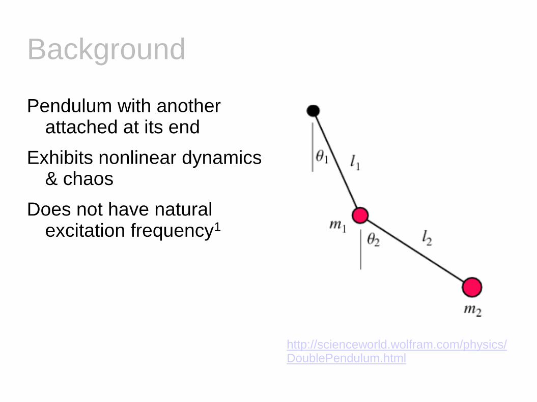
Background

Pendulum with another attached at its end

Exhibits nonlinear dynamics & chaos

Does not have natural excitation frequency1

http://scienceworld.wolfram.com/physics/DoublePendulum.html

Problem Definition

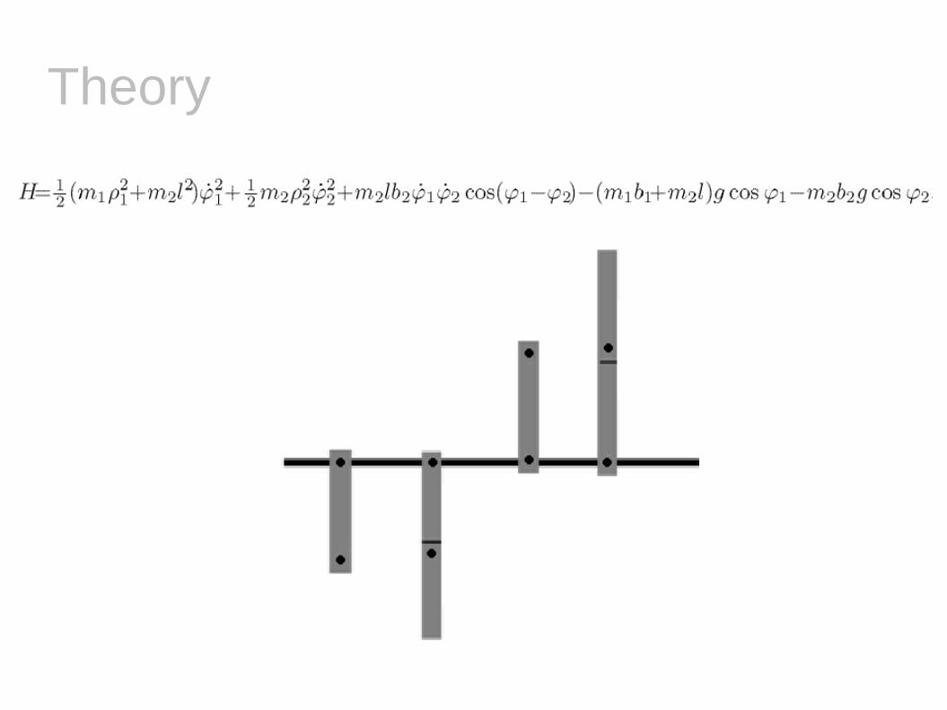
Theory

Kinetic / Potential Energy

Euler-Lagrange Equations2

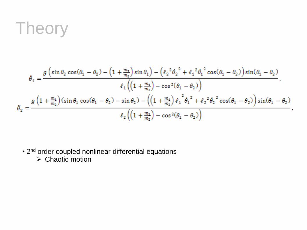
Theory

• 2nd order coupled nonlinear differential equations Chaotic motion

Theory

http://en.wikipedia.org/wiki/Double_pendulum

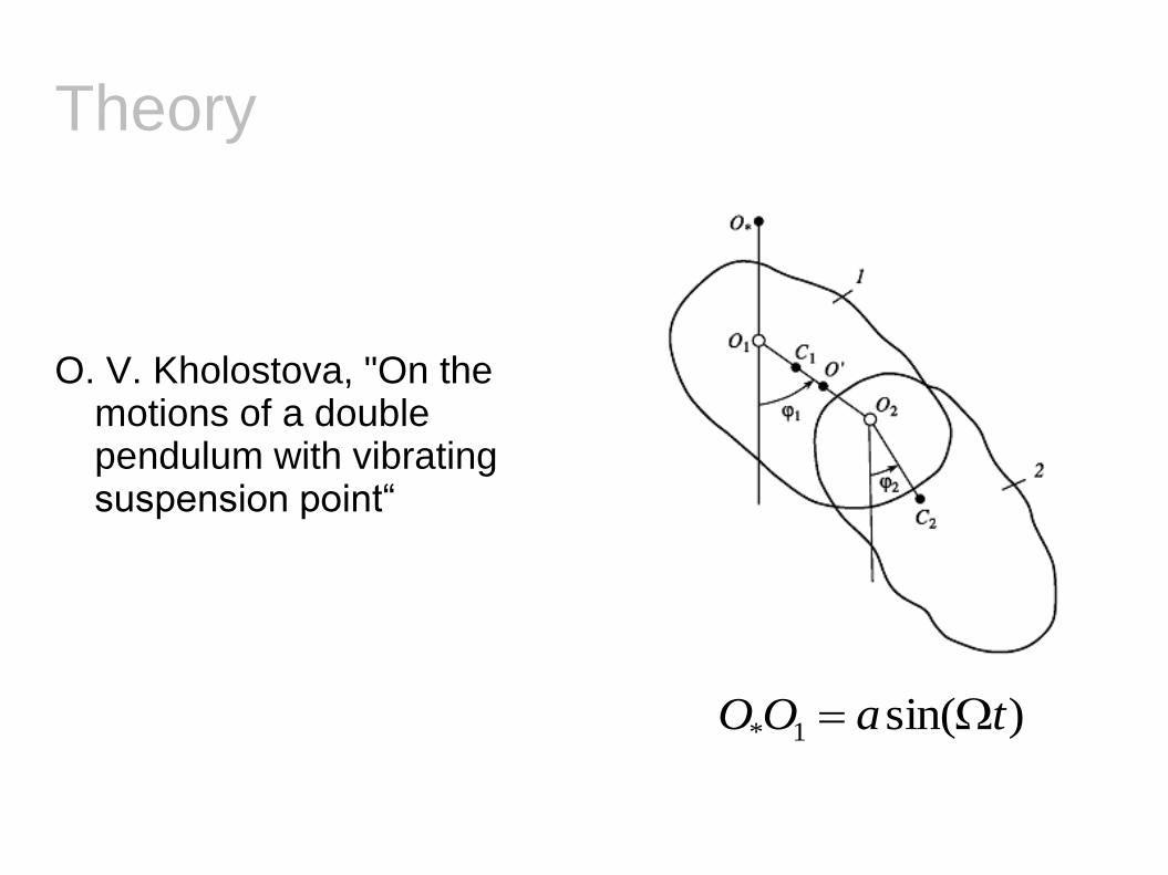
Theory

O. V. Kholostova, "On the motions of a double pendulum with vibrating suspension point“

)sin(1* taOO

Theory

O1O2 = l, O1C1 = b1 , O2C2 = b2, ρ1 and ρ2 : uniform mass density

Theory

Theory

For ‘ideal’ pendulum:

21

2121

2

2

2

1212

2 2mm

mmllllll

a

g

->The inverted pendulum is stable.

• No other stable orbits.

Theory

My contributions

Helping here and there

Website

References

1. http://en.wikipedia.org/wiki/Double_pendulum 2. Shinbrot T et al, “Chaos in a double pendulum”, Am. J. Phys. 60(6), June 1992 3. O. V. Kholostova, "On the motions of a double pendulum with vibrating suspension point," Mechanics of Solids, vol. 44, no. 2, pp. 184-197, April 2009. 4. R. B. Levien and S. M. Tan, "Double pendulum: An experiment in chaos," Am. J. Phys., vol. 61, no. 11, pp. 1038-1044, November 1993. 5. P. Qu, Q. Bi, “ANALYSIS OF NON-LINEAR DYNAMICS AND BIFURCATIONS OF A DOUBLE PENDULUM”, J. of Sound and Vibration, 217(4), 697-736, 1998

Double Pendulum: Data Collection

Michael Clark

Contributions

● Accelerometer analysis and debugging

● Driven double pendulum – initial conditions and experiment

● This section of presentation on data collection methods

Data Collection and Methods

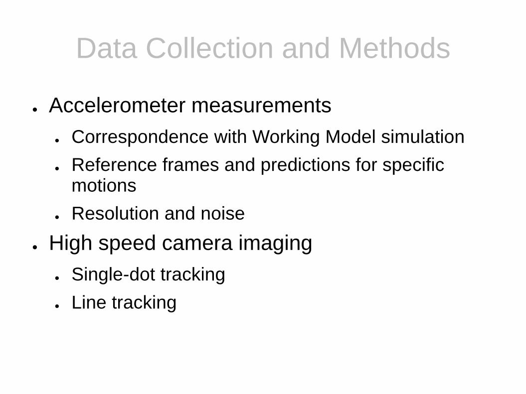
● Accelerometer measurements

● Correspondence with Working Model simulation

● Reference frames and predictions for specific motions

● Resolution and noise

● High speed camera imaging

● Single-dot tracking

● Line tracking

Accelerometer Measurements

● Analog Devices ADXL321 accelerometer

● Measures up to 18g

● Noise floor of 320μg/√Hz bandwidth

Simple Pendulum Tests

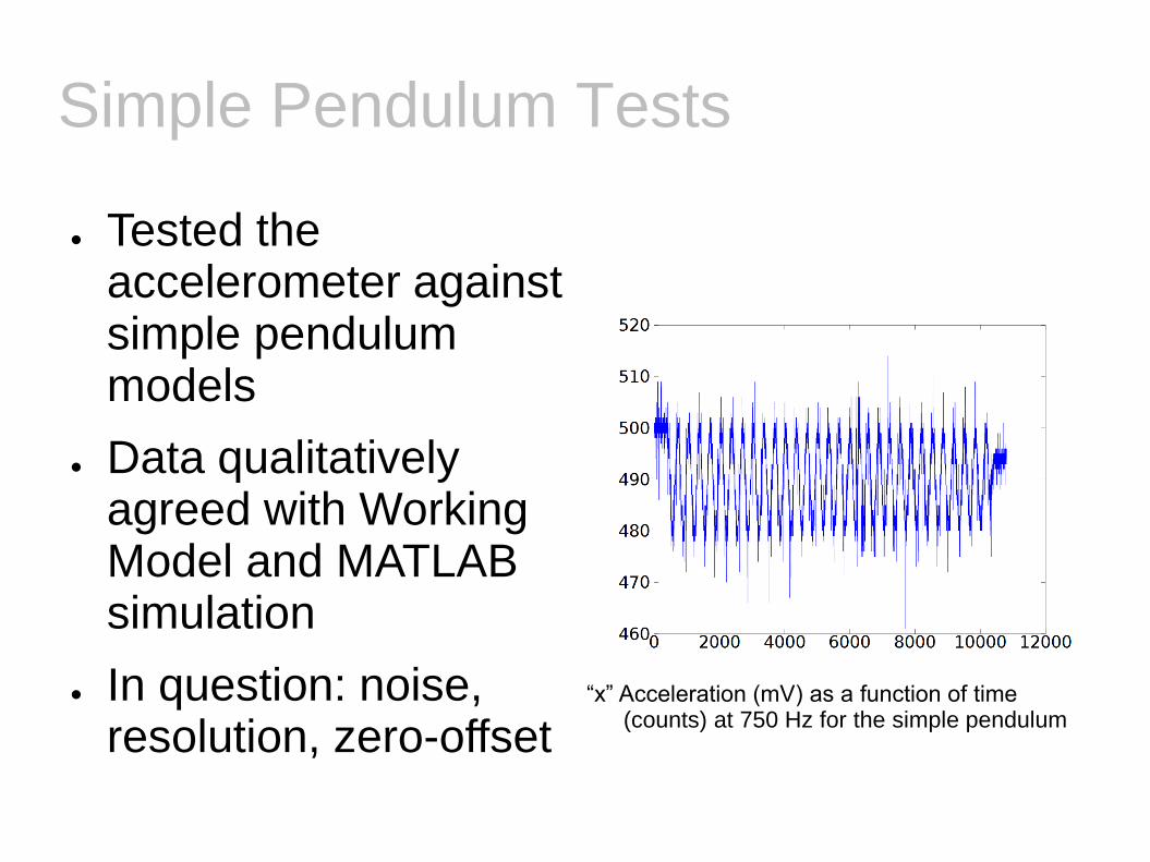
● Tested the accelerometer against simple pendulum models

● Data qualitatively agreed with Working Model and MATLAB simulation

● In question: noise, resolution, zero-offset

“x” Acceleration (mV) as a function of time (counts) at 750 Hz for the simple pendulum

d1

Coordinate Frame of Accelerometer

u

v

gravity

d2

θ1

θ2

φ=θ2-θ1 x

y

accelerometer

Accelerometer Results

● Basic geometry of the problem yields the result that (u,v)=(0,0) corresponds to (x,y)=(d2+d1cos(φ),d1sin(φ))

● It is still not a trivial task to convert a real-space trajectory to the moving, rotating frame of the accelerometer

● As a result of noise and these theoretical hurdles, we chose a different method of data collection

Video Motion Capture

● Use a high-speed (100 fps) camera to track part of the assembly

● Labview software tracks the marked point as it moves

● Real-time calculation of position and momentum

Tracking Issues

???

The tracking search box gets confused when support posts occlude the maker dot.

Solution: More Dots

● Not just more dots; a solid black line

● Costs the ability to track in real-time, but much more robust when only part of the line is blocked

● Still requires some processing when whole line is blocked

Double Pendulum: Data Processing

John Robinson

My Contributions

• Assisted in literature search

• Assisted in data collection

• Wrote and tested data processing code

Data Processing

• LabVIEW saves high-speed camera data as .bmp files

• 100 frames/second

• Convenient – no need to extract frames from video files

• Example Data:

• Step 1 – convert image to binary image using threshold

Data Processing

Data Processing

• Step 2 – convert binary image to skeleton using MATLAB Image Processing Toolkit

Data Processing

• Step 3 – perform linear regression to determine slope of skeleton

• Problem – ambiguity: two possible angles (between –pi/2 and pi/2)

Data Processing

• Solution – determine location of joint between two arms

• This can be extrapolated from slope together with information from reference images.

Location of suspension point

Length of first arm

Data Processing

Suspension point

Possible Joint Locations

Data Processing

Two possible locations for joint

Endpoint of skeleton closest to circle

Processed Data

0 200 400 600 800-1

-0.5

0

0.5

1

0 200 400 600 800-1.5

-1

-0.5

0

0.5

1

1.5Arm 1 Arm 2

Time (milliseconds) Time (milliseconds)

Angle

(ra

dia

ns)

Angle

(ra

dia

ns)

Problems

Double Pendulum w/ Oscillating Base

• Same procedure as for non-oscillating case except suspension point location varies

• Problem – poor resolution for small amplitude oscillation

Search box excluded from processing. Centroid of region determines suspension point location

Double Pendulum: Modeling

Jacob Blumoff

Contributions

• Modeling

• Hands-on work

We were inspired by this image from wikipedia. Time to flip based on initial conditions. Data collection is doable. Modeling is doable. We get to compare theory directly to data.

Main Idea

Theory Review

Integrating these would have been the best approach.

About the Model

Used WorkingModel2D and its BASIC-based internal scripting language.

Runs sets of initial (angle conditions) until the lower arm flips, or time runs out

2D Phase Space: Initial angular velocities = 0

1802 = 32,400 points

WorkingModel2D

Flaws in WorkingModel2D

It would have been much better to integrate in MATLAB or Mathematica

WorkingModel2D (scripting) only runs in real-time

Our main modeling result took ~12 hours, even with pruning.

Integrator is accurate, but only allows external code access to the data irregularly (chunky)

Flaws in the Model

We can only wait a finite time to see a flip

Not as bad as it seems

WM2D data chunkiness → limited temporal resolution (when did it flip?)

Pruning was not done correctly

Slow speed limits size and resolution

Nice Things

Time limit on how long we watch isn't that bad

We can later examine only those that didn't flip later with a longer time limit and add those points in.

It should be easy to prune some cases that will never flip, based on gravitational potential energy.

Was not implemented correctly (here)

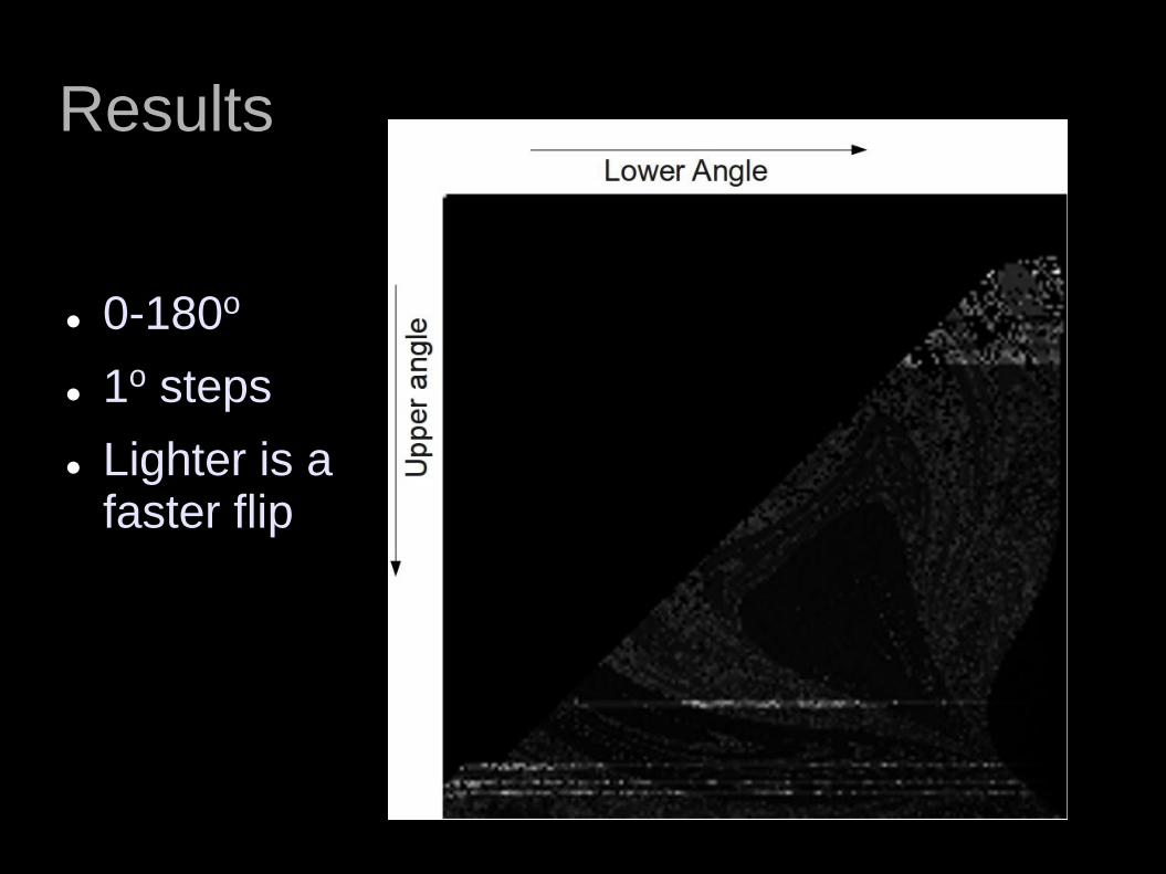
Results

0-180o

1o steps

Lighter is a faster flip

Comparison

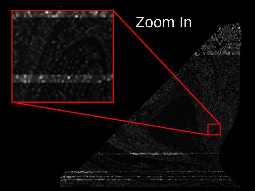
Zoom in (fractals are fun.)

Zoom In

What's Next?

Damping has been added, but not run

0-180 is all that's needed for the upper arm, by symmetry, but

We need to do -180 to 0 still for the lower arm

Better pruning (gravity) has been added, but not run

Redo the whole thing in MATLAB.