arX

iv:0

709.

1963

v3 [

astr

o-ph

] 1

8 D

ec 2

007

To appear in ApJ March 20, 2008; online at astroph http://arxiv.org/abs/0709.1963Preprint typeset using LATEX style emulateapj v. 03/07/07

DOUBLE CORONAL HARD AND SOFT X-RAY SOURCE OBSERVED BY RHESSI: EVIDENCE FORMAGNETIC RECONNECTION AND PARTICLE ACCELERATION IN SOLAR FLARES

Wei Liu1,2, Vahe Petrosian2, Brian R. Dennis1, and Yan Wei Jiang2

Received 2007 September 12; accepted 2007 December 06

ABSTRACT

We present data analysis and interpretation of an M1.4-class flare observed with the Reuven Ra-maty High Energy Solar Spectroscopic Imager (RHESSI) on April 30, 2002. This event, with itsfootpoints occulted by the solar limb, exhibits a rarely observed, but theoretically expected, double-source structure in the corona. The two coronal sources, observed over the 6–30 keV range, appear atdifferent altitudes and show energy-dependent structures with the higher-energy emission being closertogether. Spectral analysis implies that the emission at higher energies in the inner region between thetwo sources is mainly nonthermal, while the emission at lower energies in the outer region is primarilythermal. The two sources are both visible for about 12 minutes and have similar light curves andpower-law spectra above about 20 keV. These observations suggest that the magnetic reconnectionsite lies between the two sources. Bi-directional outflows of the released energy in the form of tur-bulence and/or particles from the reconnection site can be the source of the observed radiation. Thespatially resolved thermal emission below about 15 keV, on the other hand, indicates that the lowersource has a larger emission measure but a lower temperature than the upper source. This is likelythe result of the differences in the magnetic field and plasma density of the two sources.Subject headings: acceleration of particles—Sun: corona—Sun: flares—Sun: X-rays, gamma rays

1. INTRODUCTION

Magnetic reconnection is believed to be the main en-ergy release mechanism in solar flares. In the clas-sical reconnection model (e.g., Petschek 1964), mag-netic field annihilation in a current sheet producesoutflows of high speed plasma in opposite direc-tions (see Figure 1). This process can generateturbulence that accelerates particles and heats thebackground plasma stochastically (e.g., Ramaty 1979;Hamilton & Petrosian 1992; Park & Petrosian 1995;Miller et al. 1996; Petrosian & Liu 2004). Radio emis-sion and hard and soft X-rays (HXRs and SXRs) pro-duced by the high-energy particles and hot plasma areexpected to show signatures of the two oppositely di-rected outflows. Specifically, one would expect to see twodistinct X-ray sources, one above and one below the re-connection region (in the case of a vertical current sheet).

It is well established that many flares have SXR andHXR emission arising both from the source near thetop of the loop (loop-top source, e.g., Masuda 1994;Petrosian et al. 2002; Liu et al. 2004; Jiang et al. 2006;Liu 2006; Battaglia & Benz 2006) and from a pair offootpoint sources (e.g., Hoyng et al. 1981; Sakao 1994;Sui et al. 2002; Saint-Hilaire et al. 2007). The loop-topsource is believed to be near the reconnection site andproduced by freshly accelerated particles and/or heatedplasma. Observations of the expected two distinct X-raysources above and below the reconnection region havebeen rarely reported. This may be due to limited sen-sitivity, dynamic range, and/or spatial resolution of the

1 Solar Physics Laboratory (Code 671), Heliophysics Science Di-vision, NASA Goddard Space Flight Center, Greenbelt, Maryland20771; weiliu@helio.gsfc.nasa.gov

2 Center for Space Science and Astrophysics, Department ofPhysics, Stanford University, Stanford, California 94305

��������������������������������������������������������������������

Thick−target footpoints

Escaping particles

Looptop source

site emission

Turbulence accelerationregion, Coronal X−rayReconnection

Energyoutflows

Fig. 1.— Sketch of the stochastic acceleration model(Hamilton & Petrosian 1992; Park & Petrosian 1995;Petrosian & Liu 2004) proposed for solar flares. The greencurves are magnetic field lines in a possible configuration; the redcircles represent turbulence or plasma waves that are generatedduring magnetic reconnection.

instruments, because one source may be much dimmerthan the other, the two sources may be too close to-gether to be resolved, or both may be much weaker thanthe footpoints.

Sui & Holman (2003) and Sui et al. (2004) reported asecond coronal source that appeared above a strongerloop-top source in the 2002 April 15 flare and in anothertwo homologous flares. They suggested that there wasa current sheet existing between the two sources. Re-cently, in one of the events reported by Sui et al. (2004),Wang et al. (2007) discovered high speed outflows re-

2

vealed by Doppler shifts measured by the Solar Ultravi-olet Measurements of Emitted Radiation (SUMER) in-strument on board the Solar and Heliospheric Observa-tory (SOHO). This provides more evidence of magneticreconnection. Veronig et al. (2006) also found a sec-ond coronal source appearing briefly in the 2003 Novem-ber 03 X3.9 flare (Liu et al. 2004; Dauphin et al. 2006).Li & Gan (2007) reported another RHESSI flare, occur-ring on 2002 November 02, that shows a similar doublecoronal source morphology. They interpreted the twosources as thermal emission because no HXR emissionwas detected above 25 keV and the footpoints were oc-culted. In their event, however, the two sources havesomewhat different temporal evolution with the flux ofthe upper source peaking about 18 minutes later thanthat of the lower source. In radio wavelengths, Pick et al.(2005) reported a double-source structure observed inthe 2002 June 02 flare with the multi-frequency NancayRadio-heliograph (432–150 MHz). Due to its low bright-ness and/or technical difficulties, X-ray imaging spec-troscopy of the weaker coronal source was not availableor has not been studied for the above RHESSI events(Sui & Holman 2003; Sui et al. 2004; Veronig et al. 2006;Li & Gan 2007).

We report here another flare with two distinct coro-nal X-ray sources that occurred on April 30, 2002. Thebrightness of the upper source relative to the lower sourceis larger and the upper source stays longer (∼12 minutes)than those (3–5 minutes) of Sui et al. (2004). In addi-tion, the footpoints are occulted by the solar limb, andthus the spectra of the coronal sources are not contam-inated by the footpoints at high energies. This makes astronger case for the double coronal source phenomenonand allows for more detailed analysis, including X-rayimaging spectroscopy and temporal evolution of the in-dividual sources. Analysis of the decay phase of this flarewas originally reported by Jiang et al. (2006) as an exam-ple of suppression of thermal conduction and/or contin-uous heating attributed to the presence of plasma turbu-lence. Here we extend the analysis throughout the wholecourse of the flare.

Early in the flare, the two coronal sources are closetogether and the source morphology exhibits a double-cusp or “X” shape, possibly indicating where magneticreconnection takes place. As the flare evolves, the twosources gradually separate from each other. Both sourcesexhibit energy dependent structure similar to that foundfor the flares reported by Sui et al. (2004) and Liu et al.(2004). In general, for the lower source, higher-energyemission comes from higher altitudes, while the oppositeis true for the upper source. Imaging spectroscopy showsthat the two sources have very similar nonthermal com-ponents and light curves. These observations suggestthat the two HXR/SXR coronal sources are producedby intimately related populations of accelerated/heatedelectrons resulting from energy release in the same recon-nection region, which most likely lies between the twosources. These are consistent with the general pictureoutlined above. We also find that the two sources havedifferent thermal components, with a lower temperatureand larger emission measure for the lower source. Differ-ent magnetic topologies and plasma densities of the twosources can be the causes of such differences.

We present the observations and data analysis in §2

and our physical interpretation in §3. We conclude thispaper with a brief summary and discussion in §4. De-tails of specific RHESSI spectral analysis techniques areprovided in Appendix A.

2. OBSERVATIONS AND DATA ANALYSIS

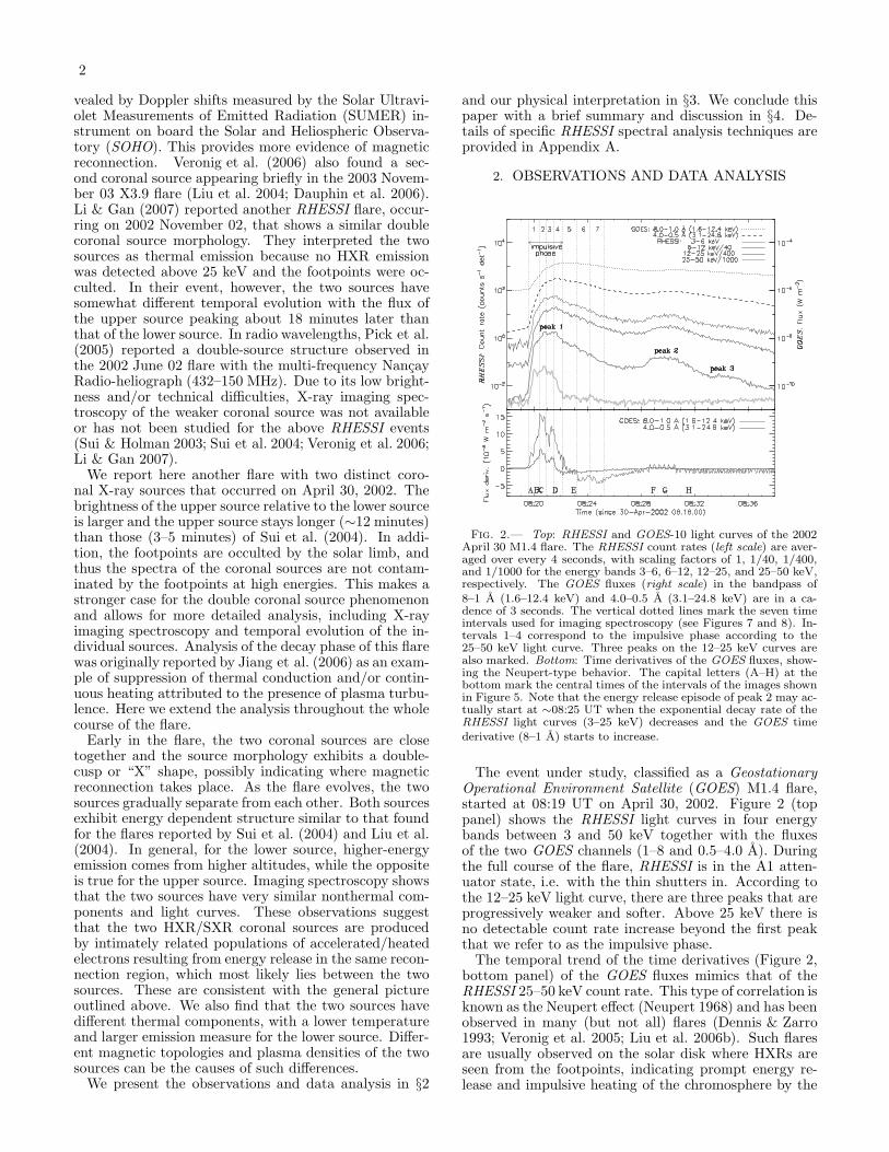
Fig. 2.— Top: RHESSI and GOES-10 light curves of the 2002April 30 M1.4 flare. The RHESSI count rates (left scale) are aver-aged over every 4 seconds, with scaling factors of 1, 1/40, 1/400,and 1/1000 for the energy bands 3–6, 6–12, 12–25, and 25–50 keV,respectively. The GOES fluxes (right scale) in the bandpass of8–1 A (1.6–12.4 keV) and 4.0–0.5 A (3.1–24.8 keV) are in a ca-dence of 3 seconds. The vertical dotted lines mark the seven timeintervals used for imaging spectroscopy (see Figures 7 and 8). In-tervals 1–4 correspond to the impulsive phase according to the25–50 keV light curve. Three peaks on the 12–25 keV curves arealso marked. Bottom: Time derivatives of the GOES fluxes, show-ing the Neupert-type behavior. The capital letters (A–H) at thebottom mark the central times of the intervals of the images shownin Figure 5. Note that the energy release episode of peak 2 may ac-tually start at ∼08:25 UT when the exponential decay rate of theRHESSI light curves (3–25 keV) decreases and the GOES timederivative (8–1 A) starts to increase.

The event under study, classified as a GeostationaryOperational Environment Satellite (GOES) M1.4 flare,started at 08:19 UT on April 30, 2002. Figure 2 (toppanel) shows the RHESSI light curves in four energybands between 3 and 50 keV together with the fluxesof the two GOES channels (1–8 and 0.5–4.0 A). Duringthe full course of the flare, RHESSI is in the A1 atten-uator state, i.e. with the thin shutters in. According tothe 12–25 keV light curve, there are three peaks that areprogressively weaker and softer. Above 25 keV there isno detectable count rate increase beyond the first peakthat we refer to as the impulsive phase.

The temporal trend of the time derivatives (Figure 2,bottom panel) of the GOES fluxes mimics that of theRHESSI 25–50 keV count rate. This type of correlation isknown as the Neupert effect (Neupert 1968) and has beenobserved in many (but not all) flares (Dennis & Zarro1993; Veronig et al. 2005; Liu et al. 2006b). Such flaresare usually observed on the solar disk where HXRs areseen from the footpoints, indicating prompt energy re-lease and impulsive heating of the chromosphere by the

3

nonthermal electrons. The hot and dense plasma re-sulting from the subsequent chromospheric evaporation(Neupert 1968) then fills the loop and gives rise to thegradual SXR increase (Liu 2006, Chapter 83). In thisflare, however, the footpoints are occulted by the limb(as we show below). Thus, the presence of the Neu-pert effect here implies that the coronal impulsive HXRsare produced by the same nonthermal electrons that fur-ther propagate down to the footpoints and drive chro-mospheric evaporation there.

Fig. 3.— RHESSI PIXON images in different energy bands at08:20:27–08:20:56 UT (interval 2 in Figure 2), around the maxi-mum of the main (first) HXR peak. We used the PIXON back-ground model and detectors 3–6 and 8, which yield a resolution of∼ 4.′′6 determined from the FWHM of the point spread functionobtained by simulation. Note that the PIXON algorithm, underfavorable conditions, can achieve a resolution as small as a fraction(see Aschwanden et al. 2004, §A8) of the FWHM resolution of thefinest detector used (6.′′8 for detector 3 in our case). The contourlevels are 10%, 30%, 50%, 70%, and 90% of the maximum, I max

(shown in the upper left corner of each panel, in units of photonscm−2 s−1 arcsec−2), of each individual image. The numbers in thelower right corners are the total counts accumulated by the detec-tors used for image reconstruction. The heliographic grid spacingis 1◦. The boxes shown in the 14–16 keV panel are used to obtainthe fluxes and centroids of the two sources in all the images at thistime (see text). The two black dashed lines in the 10–12 keV panelforming an “X” show the possible configuration of the reconnectingmagnetic field.

The spatial morphology of the flare is shown in Figure 3in X-rays and in Figure 4 in EUV. Figure 3 shows PIXON(Metcalf et al. 1996; Hurford et al. 2002) images at dif-ferent energies integrated over the interval of 08:20:27–08:20:56 UT (marked #2 in Figure 2) during the firstHXR peak. As can be seen, this flare occurred on theeast limb, and the X-ray emission at all energies (even ashigh as 39–50 keV) appeared above the limb, suggestingthat the footpoints were occulted. This conclusion is sup-ported by SOHO observations shown in Figure 4. Thetop left panel shows an EUV Imaging Telescope (EIT)195 A image taken at 08:22:58 UT (just two minutes afterthe RHESSI images in Figure 4). The red contours arefor the RHESSI image at 9–10 keV shown in Figure 3.

3 Available at http://sun.stanford.edu/∼weiliu/thesis/wei thesis.pdf.

Fig. 4.— Upper left: SOHO/EIT 195 A image at 08:22:58 UTin the background, superimposed with RHESSI contours in red at9–10 keV and 08:20:27–08:20:56 UT. The insert shows the zoomedview of the RHESSI source and co-spatial EIT emission (with adifferent color scale for better contrast). Upper right: SOHO/MDImagnetogram taken at 21:20 UT (some 13 hours after the flare),overplotted with the same RHESSI 9–10 keV contours in red. TheNOAA active regions (ARs) are labeled. The heliographic gridspacing is 10◦ in the two upper panels. Lower left: Overlay ofimages, same as those shown in Figure 3, in three energy bands asindicated in the legend. The contour levels are at 17% & 80% (9–10 keV), 47% & 90% (14–16 keV), and 80% & 90% (16–19 keV) ofthe maximum brightness of individual images. In each image, twocontours appear in the lower coronal source, while only the lower-level contour is present in the upper source because of its faintness.The two plus signs mark the centroids (separated by 4.′′6± 0.′′3) ofthe lower and upper 16–19 keV sources inside the 90% and 80%contours, respectively. The heliographic grid spacing is 1◦. Lowerright: Height above the limb of the centroids for the upper andlower coronal sources plotted as a function of energy for time in-tervals 1–4 marked in Figure 2. Note that during the first interval,only one source is detected and is shown as the lower source. Forclarity, uncertainties are shown for only one time interval for thelower source and they are similar at other times.

The RHESSI source is co-spatial with the brighteningin the EIT image, which is clearly above the limb. Theflare occurred near the region where large-scale trans-equatorial loops are rooted, presumably behind the limb.There was no brightening on the disk detected by EIT,nor was an active region seen in the SOHO MichelsonDoppler Imager (MDI) magnetograms in the vicinity ofthis flare. EIT and MDI have spatial resolutions of 2.′′6and 4′′, respectively, both better than the 6.′′8 resolutionof the finest RHESSI detector (#3) used here. The topright panel of Figure 4 shows the MDI magnetogram at21:20 UT, about 13 hours after the flare. At this time,NOAA AR 9934 had just appeared on the disk next tothe RHESSI source due to the solar rotation. This sug-gests that the flare took place in this active region whenit was still behind the limb. Because of the large size ofthe active region, it is difficult to determine the possiblelocations of the footpoints of the flare and to estimatethe approximate altitudes of the coronal sources.

2.1. Source Structure: Energy Dependence

Let us now return to Figure 3 and examine in detail theenergy-dependent morphology of the flare. At the lowestenergy shown (7–8 keV), there are two distinct sources,which we call the lower and upper coronal sources. The

4

centroids of both sources are above the solar limb, andthe upper source is dimmer. At a slightly higher en-ergy, 9–10 keV, the sources appear closer together and acusp shape develops between them. This trend is morepronounced at higher energies (10–19 keV) and the twosources (particularly the lower one) seem to have a fea-ture convex toward each other, mimicking the “X” shapeof the magnetic field lines in the standard reconnectionmodel. Meanwhile, the relative brightness of the uppersource increases with energy.

The change in source altitude with energy is shownmore clearly in the lower left panel of Figure 4. Theupper coronal source shifts toward lower altitudes withincreasing energy while the lower coronal source behavesoppositely. At 16–19 keV, the two sources, while beingspatially resolved, are closest together with their cen-troids separated by 4.′′6 ± 0.′′3 (see Figure 4, lower left).

We can appreciate this more quantitatively by look-ing at the heights (above the limb) of the centroids ofthe upper and lower coronal sources as a function ofenergy. This is shown in the lower right panel of Fig-ure 4. The boxes depicted in the middle panel of Fig-ure 3 were used to obtain the centroid positions. Theerror bars were obtained from the centroid position un-certainties in the same images reconstructed with thevisibility-based forward-fitting algorithm currently avail-able in the RHESSI software. The energy-dependent pat-tern is clearly present; that is, the centroid of the upper(lower) source shifts to lower (higher) altitudes with in-creasing energy. We note that, at very high energies(& 20 keV), this pattern becomes obscure (see Figures 3and 4), but the uncertainties in the source locations be-come large due to low count rates.

Three other time intervals during the first HXR peakwere also analyzed and the results are plotted in Figure 4,exhibiting similar patterns. At the very beginning of theflare (08:19:37–08:20:27 UT), only one source is visibleand we assign its centroid (black triangles) to the lowersource since it is the main source. As mentioned earlier,the second and third HXR peaks are weaker and softer,which does not allow for this kind of detailed analysiswith narrow energy bins. We defer our physical interpre-tation of these observations to §3.1.

2.2. Source Structure: Temporal Evolution

We now change our perspective, using relatively widerenergy bins as a trade-off for finer time resolution (com-pared with the above analysis), and examine the tempo-ral evolution of the source structure throughout the fullcourse of the flare.

Figure 5 shows the PIXON images taken at 6–9, 9–12, 12–16 and 16–25 keV at eight separate times (la-beled A–H in Figure 2). The morphology evolves follow-ing the general trend mentioned above. Early (08:19:28-08:20:01 UT, interval A) in the flare, only a single sourceis visible. During the next time interval (B), the up-per coronal source appears at 6–9 keV, but only a singlesource is evident at higher energies albeit with elongatedshapes. In interval C, two distinct coronal sources ap-pear in a dumb-bell shape at all the energies. As timeproceeds, both sources move to higher altitudes. Thismorphology is present for about 12 minutes (from 08:20to 08:32 UT) until the declining phase of the second peakwhen only one source is detected, possibly because of

Fig. 5.— PIXON images of different energies made with de-tectors 3–6 and 8 at selected times (i.e., intervals A–H as markedin Figure 2). In each panel, the gray-scale background is at 6–9 keV, while the red, green and blue contours (20% and 70% ofthe peak flux of each image) are at 9–12, 12–16 and 16–25 keV,respectively. The heliographic grid spacing is 2◦. The last panelshows the locations of the centroids of the lower and upper 6–9 keVsources at different times indicated by the color bar. The dashedline indicates the radial direction (perpendicular to the limb). Themagenta and green arrows point to the centroid locations at thetimes of the first and second HXR peaks, respectively.

the faintness of the upper source and the low count rate.Note that after 08:29 UT the upper source is dimmerthan 20% of the maximum of the image and thus doesnot appear in panels G and H.

The motions of the sources can be seen more clearlyfrom the migration of the centroids. To obtain the cen-troids and fluxes of the sources, we use contours whoselevels are equal to within 5% of the minimum betweenthe two sources so that the contours of the two sourcesare independent. The last panel in Figure 5 shows theevolution of the centroid positions of the two sources at6–9 keV. During the first HXR peak (indicated by the

5

magenta arrow), the lower coronal source first shifts tolower altitudes and then ascends. This is consistent withthe decrease of the loop-top height early during the flareobserved in several other events (Sui & Holman 2003;Liu et al. 2004; Sui et al. 2004). Meanwhile, the uppersource generally moves upwards. Such centroid motionsare also present at other energies as shown in the lowerright panel of Figure 4. The reversal of the lower sourcealtitude seems to happen again, but less obvious, duringthe second peak (marked by the green arrow).

We can examine the same phenomenon more quanti-tatively by checking the height of the source centroid asa function of time at different energies. This is shown inFigure 6a for the upper (left scale) and lower (right scale)coronal sources. We find that, again, the higher-energyemission comes from lower altitudes for the upper sourceand the lower source shows the opposite trend. The onlyexception (indicated by the dashed box) to this generalbehavior occurs for the upper source during the late de-clining phase of first HXR peak and during the secondand third peaks when there are large uncertainties be-cause of low count rates.

At 6–9 keV (red symbols), the altitude of the lowersource first decreases at a velocity of 10±2 kms−1, whilethe altitude of the upper source increases at a veloc-ity of 52 ± 18 kms−1. These are indicated by linear fits(red solid line) during the high flux period. This hap-pens during the rising phase (up to 08:21:14 UT) of thefirst HXR peak and is followed by an increase of thealtitudes of the two sources with comparable velocities(15±1 kms−1 and 17±4 kms−1 for the lower and uppersources, respectively) during the early declining phase(up to 08:22:59 UT). As time proceeds, the two sourcesgenerally continue to move to higher altitudes. The ve-locity of the lower source drops to 7.6 ± 0.5 kms−1 until08:28:56 UT, around the maximum of the second HXRpeak, and then to 2.3 ± 0.6 kms−1 afterwards. The ve-locity of the upper source also decreases in general, withsome fluctuations most likely due to the large uncertain-ties mentioned above. The relative motion of the twosources can be seen from the temporal variation of thedistance between their centroids as shown in Figure 6b(red asterisks), which undergoes a fast initial increaseand then stays roughly constant at 15′′ ± 1′′ within theuncertainties.

At 12–16 (green) and 16–25 keV (blue), the centroidshave a trend similar to those at 6–9 keV, except for thelower coronal source during the early rising phase of thefirst HXR peak. The initial increase of the height ofthe “lower”4 source at about 08:20 UT results from theelongation (see the second panel in Figure 5) of the sin-gle source, which could be a combination of the lowerand upper sources that are not resolved. The followingrapid decrease in height in the next time interval is aconsequence of the transition from a single-source to adouble-source structure as mentioned earlier. The uppersource, on the other hand, rises more rapidly than at 6–9 keV during the HXR rising and early declining phases.Its velocity at 16–25 keV, for example, is 32 ± 3 kms−1

during the interval of 08:21:14–08:22:59 UT. This en-ergy dependence of the rate of rise is consistent with the

4 Again, we assign its centroid to the lower source when there isonly a single source detected.

general trend of the loop-top source observed in severalother flares (Liu et al. 2004; Sui et al. 2004). We note inpassing that, in addition to the first HXR peak (markedwith D1 in Figure 6), the altitudes of the lower sourcecentroids also appear to first decrease and then increaseduring two other time periods5 (D2 and D3). This effectis most pronounced at 12–16 and 16–25 keV.

Fig. 6.— (a) Height (above the limb) of the centroids at differentenergies for the upper (left scale) and lower (right scale) coronalsources. The dotted vertical lines separate the different phases ac-cording to the motion of the lower source centroid (see text). Thered solid lines are linear fits to the data during the correspondingtime intervals, with the adjacent red numbers indicating the veloc-ities of the altitude gain in units of km s−1. The centroid positionof the upper source has large fluctuations and uncertainties duringthe interval marked by the dashed box. The letters D1, D2, andD3 mark the times when the altitude of the lower source decreases.(b) Left scale: Distance (red asterisks) between the centroids of thetwo coronal sources at 6–9 keV and separation (diamonds) betweenthe centroids of the lower source at 6–9 and 16-25 keV. The formeris shifted downwards by 9′′. Right scale: Base-10 logarithm of thespatially integrated light curve (counts s−1 detector−1, thin line)at 12–25 keV. (c) Light curves of the upper (dashed) and lower(solid) coronal sources in the energy bands of 6–9, 12–16, and 16–25 keV (divided by 10). The same contours (see text) were usedto obtain these light curves and the centroid positions in panel a.

2.3. Spectral Evolution

In this section, we examine the relationship betweenthe fluxes and spectra of the two coronal sources. Fig-ure 6c shows the photon flux evolution at 6–9, 12–16,

5 D3 coincides with the second HXR peak and D2 occurs around08:25 UT, which is the possible actual start of the second energy re-lease episode (see Figure 2), when the upper source also appears toshow a significant decrease in centroid altitude. Such altitude vari-ations seem to be associated with the possible increases of energyrelease rate indicated by the light curves. However, compared withD1, the features at the two later times are less definitive given therelatively fewer data points and larger uncertainties of the centroidheights.

6

and 16–25 keV. As evident, the fluxes of the two sourcesbasically follow the same time variation in all three en-ergy bands. The upper coronal source, however, appearslater and disappears earlier, presumably due to its faint-ness and the limited RHESSI dynamic range (∼10:1). Italso peaks later at 6–9 keV.

We also conducted imaging spectroscopic analysis foreach of the seven time intervals defined in Figure 2. Thespectra of the two sources separately and the spatiallyintegrated spectra were fitted with a single-temperaturethermal spectrum plus a power-law function. One im-portant step was to fit the spatially integrated spectraof individual detectors separately and then average theresults in order to obtain the best-fit parameters andtheir uncertainties. Interested readers are referred to Ap-pendix A for the technical details of the spectrum fittingprocedures used to obtain the results reported here.

Fig. 7.— Spectra of the lower and upper coronal sources andthe spatially integrated spectra (labeled as “total”) at four timesduring the major flare peak. The numbers (2, 3, 4, and 5) inthe upper-right corners correspond to the numbered time inter-vals shown in Figure 2. The upper source’s spectra and the totalspectra have been shifted downwards by one and three decades,respectively. The horizontal error bars represent the energy binwidths and the vertical error bars are the statistical uncertaintiesof the spectra. The best fit to the data with a thermal plus power-law model is shown as the dotted (dashed) line for the lower (upper)source. The thermal (dotted) and power-law (dashed) componentsof the best fit to the total spectra are also shown. The legendindicates the corresponding power-law indexes (γ) for each spec-trum (γ = 2 below the low cutoff energy). The lower portion ofeach panel shows the ratio of the upper to lower fluxes (asterisksymbols, left scale), and the residuals (solid lines, right scale) ofthe fit to the spatially integrated spectra, normalized to the 1σuncertainty of the measured flux at each energy.

A sample of the resulting spectra of four intervals isshown in Figure 7. Fits to the spatially integrated spec-tra indicate that the low-energy emission is dominated bythe thermal components, while the nonthermal power-law components dominate at high energies. The twocomponents cross each other at an energy that we callE cross. The spectra of the two coronal sources measuredseparately have similar slopes. In general, the ratio ofthe two spectra (upper source/lower source) is smaller

than unity and gradually increases with energy belowaround E cross. This trend can also be appreciated by not-ing the increasing relative brightness of the upper sourcewhen energy increases as shown in Figure 3. This energy-dependent variation of the flux ratio means that the ther-mal emissions of the two sources are somewhat differentnot only in emission measure (EM) but also in temper-ature, because different EMs alone would only affect thenormalizations and produce a flux ratio that is indepen-dent of energy. We also note that above E cross, the ra-tio stays constant within the larger uncertainties. Thismeans that the nonthermal spectra of the two sourceshave similar power-law indexes (see Figure 8a).

The reduced χ2 values of the spatially integrated spec-tra are somewhat large (&2) partly because we set thesystematic uncertainties to be zero as opposed to the de-fault 2%. Another reason was that we averaged the pho-ton fluxes and best-fit parameters over different detectorsthat have slightly different characteristics. Thus, the av-eraged model may not necessarily be the best fit to theaveraged data (see §A.1, item 9), although the χ2 valuesof the fits to the individual detectors are usually close tounity. The normalized residuals exhibit some systematic(non-random) variations, as shown in the bottom portionof each panel of Figure 7. This suggests that simple spec-trum form adopted here may not represent all the detailsof the data. However, since we are mainly concerned withthe similarities and differences between the spectra of thetwo coronal sources, such systematic variations would af-fect both spectra the same way and thus will not alterour major conclusions. More sophisticated techniques,such as the regularization method (Kontar et al. 2004),can be used to obtain better fits to the data, but theyare beyond the scope of this paper.

We now examine the temporal evolution of variousspectral characteristics as shown in Figure 8. Let usfocus on the late impulsive phase outlined by the twovertical dotted lines6. Again, we find that the power-lawindexes (Figure 8a) of the two coronal sources are veryclose, with a difference of ∆γ ≤ 0.7. The two spectraundergo continuous softening during this stage, and thespatially integrated spectrum follows the same generaltrend.

Figures 8b and 8c show that the thermal emissions ofthe two sources are quite different as noted above. Thelower coronal source has a larger emission measure butlower temperature than the upper source. As time pro-ceeds, both sources undergo a temperature decrease andemission measure increase. This must be the result ofthe interplay of continuous heating, cooling by conduc-

6 Beyond the time interval between the two vertical lines in Fig-ure 8, i.e., during the early impulsive phase (before 08:20:27 UT)and the decay phase (after 08:22:08 UT), interpretation of the spec-tral fitting needs to be taken with caution because of the large un-certainties due to low count rates and thus relatively poor statis-tics. Specifically, during certain intervals, reliable power-law com-ponents from fits to the spatially resolved spectra could not be ob-tained and thus the corresponding values of the spectral index (γ)and thermal-nonthermal cross-over energy (E cross) are not shownin Figure 8. In addition, the averages of the best-fit parametersof the two sources differ significantly from the corresponding val-ues of the spatially integrated spectrum. This is unexpected andmay indicate that there existed an extended source with low-surfacebrightness and/or that the fits to the imaged spectra at these timesare not reliable. Nevertheless, we show the fitting results here forcompleteness.

7

Fig. 8.— Evolution of various spectroscopic quantities of thelower (asterisks) and upper (diamonds) coronal sources and thespatially integrated emission (pluses, labeled “total”). The hori-zontal error bars represent the widths of the time intervals of in-tegration as labeled (1–7) in panel b (also in Figure 2). The twovertical dotted lines mark the boundaries of the time range whenboth coronal sources are best imaged. This spans the late impulsivephase (see the 25–50 keV light curve). Before and after this timerange the imaging spectroscopy has relatively large uncertainties(see text). (a) Spectral indexes (symbols, left scale) of the power-law components of the model fits, together with the 12–25 and25–50 keV light curves (solid lines, right scale). (b) and (c) Emis-sion measures (in 1049 cm−3) and temperatures (in 106 K) of thethermal components of the model fits. (d) The cross-over energy,E cross, at which the thermal and power-law components are equal.Note that the values here are the upper limits of E cross. This isbecause we assumed a γ = 2 index for the photon spectrum belowthe low-energy cutoff, but the power-law component may extendto low energies with a steeper index thus lowering the values ofE cross.

tion and radiation, and heat exchange between regions ofdifferent temperatures within the emission source. Notethat the temperature and emission measure of the spa-tially integrated spectrum, as expected, lie between thoseof the two sources.

We can further estimate the densities of the two sourcesusing their EMs and approximate volumes. Assumingthat the sources are spheres and using the 6.′′3 and 5.′′2FWHM source sizes obtained from the visibility forwardfitting images as the diameters, we obtained the volumes,V . We then estimated the lower limits of the densities(n =

√

EM/[V f ], assuming a filing factor f of unity) ofthe lower and upper sources at 08:20:27-08:20:56 UT tobe 2.4 × 1011 and 8.0 × 1010 cm−3, respectively.

Figures 8d shows the history of the cross-over energyE cross. In general, the lower source has a lower E cross be-cause of its lower temperature. The E cross values of bothsources increase with time because the thermal emissionbecomes increasingly dominant, as seen in many otherflares. Physical interpretation of these observations ispresented in the next section.

3. INTERPRETATION AND DISCUSSION

3.1. Energy Dependence of Source Structure

The energy-dependent source morphology presented in§2.1 (see Figure 4, lower left) is similar to that reportedby Sui & Holman (2003) and Sui et al. (2004) and in-terpreted as magnetic reconnection taking place betweenthe two coronal sources. In their interpretation, plasmawith a higher temperature is located closer7 to the re-connection site than plasma with a lower temperature.This can result in higher-energy emission coming from aregion closer to the reconnection site while lower-energyemission comes from a region further away, provided thatthe emission is solely produced by thermal emission (free-free and free-bound) and the lower-temperature plasmahas a higher emission measure.

Our interpretation is somewhat different, particularlyfor this flare. Regardless of the emission nature (ther-mal or nonthermal) of the HXRs, the energy-dependentsource structure here simply means harder (flatter) pho-ton spectra closer to the reconnection site, which cangive rise to a higher weighting there at high energies forthe centroid calculations. A larger spatial gradient of thespectral hardness would lead to a larger separation of theemission centroids at two given photon energies, and azero gradient (uniform spectrum) means no separation.As we have seen in §2.3, both coronal sources have sub-stantial power-law (presumably nonthermal) tails (Fig-ure 7), which makes a purely thermal interpretation im-probable. In the framework of the stochastic accelerationmodel (Hamilton & Petrosian 1992; Miller et al. 1996),one expects both heating of plasma and acceleration ofparticles into a nonthermal tail to take place. As shownin Petrosian & Liu (2004), higher levels of turbulencetend to produce harder electron spectra or more acceler-ation and less heating. One expects a higher turbulencelevel near the X-point of the reconnection site than fur-ther away. Consequently, there will be more accelerationand thus stronger nonthermal emission near the center,but more heating and thus stronger thermal emission fur-ther away from the X-point. In other words, the electronspectra and thus the observed photon spectra will beharder closer to the reconnection site. This physical pic-ture is sketched in Figure 9.

The observations here support the above scenario. Asshown in Figure 7, below the critical energy E cross (say,∼15 keV for 08:20:27–08:20:56 UT), the emission is dom-inated by the thermal component, and the two sourcesare further apart at lower energies (see Figure 4, lowerpanels). This translates to the outer region away fromthe center of the reconnection site being mainly thermalemission at low energies. Above E cross, on the otherhand, the power-law component dominates. The twosources being closer together at higher energies8 thusmeans that the region near the center is dominated by

7 Sui & Holman (2003) also suggested a possible transition atabout 17 keV from the thermal flare loops to the Masuda-typeabove-the-loop HXR source (Masuda et al. 1994), on the basis ofthe sudden displacement of the loop-top source position in the 2002April 15 flare.

8 At even higher energies (&25 keV), the distance between thetwo sources seems to increase, but with larger uncertainties (Fig-ure 4, lower right). This transition, if real, may suggest that trans-port effects become important. This is because higher-energy elec-trons require greater column depths to stop them, and thus theytend to produce nonthermal bremsstrahlung emission at larger dis-tances from where they are accelerated.

8

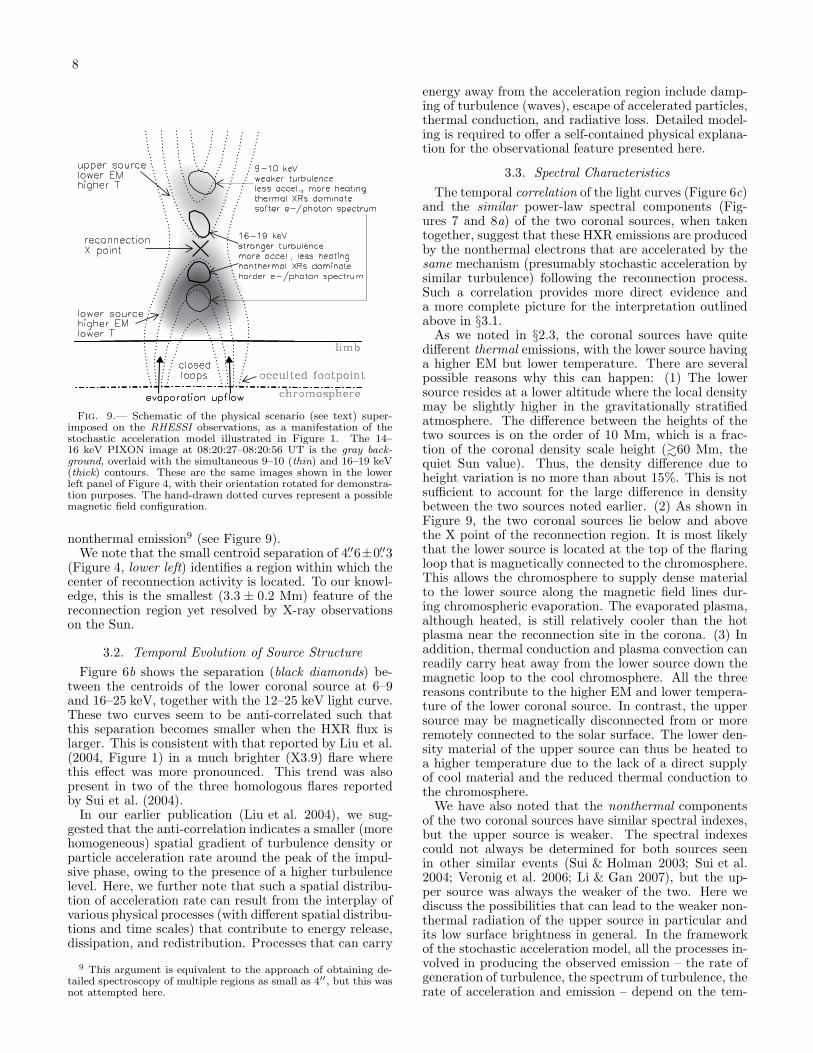
Fig. 9.— Schematic of the physical scenario (see text) super-imposed on the RHESSI observations, as a manifestation of thestochastic acceleration model illustrated in Figure 1. The 14–16 keV PIXON image at 08:20:27–08:20:56 UT is the gray back-ground, overlaid with the simultaneous 9–10 (thin) and 16–19 keV(thick) contours. These are the same images shown in the lowerleft panel of Figure 4, with their orientation rotated for demonstra-tion purposes. The hand-drawn dotted curves represent a possiblemagnetic field configuration.

nonthermal emission9 (see Figure 9).We note that the small centroid separation of 4.′′6±0.′′3

(Figure 4, lower left) identifies a region within which thecenter of reconnection activity is located. To our knowl-edge, this is the smallest (3.3 ± 0.2 Mm) feature of thereconnection region yet resolved by X-ray observationson the Sun.

3.2. Temporal Evolution of Source Structure

Figure 6b shows the separation (black diamonds) be-tween the centroids of the lower coronal source at 6–9and 16–25 keV, together with the 12–25 keV light curve.These two curves seem to be anti-correlated such thatthis separation becomes smaller when the HXR flux islarger. This is consistent with that reported by Liu et al.(2004, Figure 1) in a much brighter (X3.9) flare wherethis effect was more pronounced. This trend was alsopresent in two of the three homologous flares reportedby Sui et al. (2004).

In our earlier publication (Liu et al. 2004), we sug-gested that the anti-correlation indicates a smaller (morehomogeneous) spatial gradient of turbulence density orparticle acceleration rate around the peak of the impul-sive phase, owing to the presence of a higher turbulencelevel. Here, we further note that such a spatial distribu-tion of acceleration rate can result from the interplay ofvarious physical processes (with different spatial distribu-tions and time scales) that contribute to energy release,dissipation, and redistribution. Processes that can carry

9 This argument is equivalent to the approach of obtaining de-tailed spectroscopy of multiple regions as small as 4′′, but this wasnot attempted here.

energy away from the acceleration region include damp-ing of turbulence (waves), escape of accelerated particles,thermal conduction, and radiative loss. Detailed model-ing is required to offer a self-contained physical explana-tion for the observational feature presented here.

3.3. Spectral Characteristics

The temporal correlation of the light curves (Figure 6c)and the similar power-law spectral components (Fig-ures 7 and 8a) of the two coronal sources, when takentogether, suggest that these HXR emissions are producedby the nonthermal electrons that are accelerated by thesame mechanism (presumably stochastic acceleration bysimilar turbulence) following the reconnection process.Such a correlation provides more direct evidence anda more complete picture for the interpretation outlinedabove in §3.1.

As we noted in §2.3, the coronal sources have quitedifferent thermal emissions, with the lower source havinga higher EM but lower temperature. There are severalpossible reasons why this can happen: (1) The lowersource resides at a lower altitude where the local densitymay be slightly higher in the gravitationally stratifiedatmosphere. The difference between the heights of thetwo sources is on the order of 10 Mm, which is a frac-tion of the coronal density scale height (&60 Mm, thequiet Sun value). Thus, the density difference due toheight variation is no more than about 15%. This is notsufficient to account for the large difference in densitybetween the two sources noted earlier. (2) As shown inFigure 9, the two coronal sources lie below and abovethe X point of the reconnection region. It is most likelythat the lower source is located at the top of the flaringloop that is magnetically connected to the chromosphere.This allows the chromosphere to supply dense materialto the lower source along the magnetic field lines dur-ing chromospheric evaporation. The evaporated plasma,although heated, is still relatively cooler than the hotplasma near the reconnection site in the corona. (3) Inaddition, thermal conduction and plasma convection canreadily carry heat away from the lower source down themagnetic loop to the cool chromosphere. All the threereasons contribute to the higher EM and lower tempera-ture of the lower coronal source. In contrast, the uppersource may be magnetically disconnected from or moreremotely connected to the solar surface. The lower den-sity material of the upper source can thus be heated toa higher temperature due to the lack of a direct supplyof cool material and the reduced thermal conduction tothe chromosphere.

We have also noted that the nonthermal componentsof the two coronal sources have similar spectral indexes,but the upper source is weaker. The spectral indexescould not always be determined for both sources seenin other similar events (Sui & Holman 2003; Sui et al.2004; Veronig et al. 2006; Li & Gan 2007), but the up-per source was always the weaker of the two. Here wediscuss the possibilities that can lead to the weaker non-thermal radiation of the upper source in particular andits low surface brightness in general. In the frameworkof the stochastic acceleration model, all the processes in-volved in producing the observed emission – the rate ofgeneration of turbulence, the spectrum of turbulence, therate of acceleration and emission – depend on the tem-

9

perature, density, and the magnetic field strength andgeometry. As we mentioned above, the temperature,density, and field geometry of the two coronal sourcesare different. The magnetic field strength most likely de-creases with height. Consequently, we expect differentHXR intensities from the two sources. For example, thelower plasma density in the upper source will result inlower surface brightness for both thermal and nonther-mal bremsstrahlung emission. Magnetic topology canhave similar effects. The electrons responsible for theupper source are likely to be on open field lines or onfield lines that connect back to the chromosphere moreremotely (e.g., Liu et al. 2006a) and thus produce theirX-ray emission in a more spatially diffuse region. In con-trast, for the lower source, the electrons are confined inthe closed loop. In addition, as noted above, chromo-spheric evaporation can further increase the density inthe loop, enhancing the density effect mentioned here.These factors, again, lead to lower surface brightness forthe upper source. Finally, the rate of acceleration orheating depends primarily on the strength of the mag-netic field (Petrosian & Liu 2004), so that the relativelyweaker magnetic field of the upper source may result inslower acceleration and thus weaker nonthermal emis-sion. A large sample of this type of flares is required toconfirm or reject this explanation.

We should emphasize that since the radiating electronsin both sources are the direct product of the same accel-eration mechanism, they share common signatures. Thiswould explain the spectral similarity of the nonthermalemissions of the two coronal sources. The thermal X-ray emitting plasma, however, in addition to direct heat-ing by turbulence, involves many other indirect or sec-ondary processes, such as cooling by thermal conductionand hydrodynamic effects (e.g., evaporation in the closedloop). Therefore, the two thermal sources exhibit rela-tively large differences in their temperatures and emis-sion measures.

4. CONCLUDING REMARKS

We have performed imaging and spectral analysis ofthe RHESSI observations of the M1.4 flare that oc-curred on April 30, 2002. Two correlated coronal HXRsources appeared at different altitudes during the impul-sive and early decay phases of the flare. The long du-ration (∼12 minutes) of the sources allows for detailedanalysis and the results support that magnetic reconnec-tion and particle acceleration were taking place betweenthe two sources. Our conclusions are as follows.

1. Both coronal sources exhibit energy-dependentmorphology. Higher-energy emission comes fromhigher altitudes for the lower source, while the op-posite is true for the upper source (Figures 3 and4). This suggests that the center of magnetic recon-nection is located within the small region betweenthe sources.

2. The energy-dependent source structure (Figure 4),combined with spectrum analysis (Figure 7), im-plies that the inner region near the reconnectionsite is energetically dominated by nonthermal emis-sion, while the outer region is dominated by ther-mal emission. This observation, in the framework

of the stochastic acceleration model developed byHamilton & Petrosian (1992) and Petrosian & Liu(2004), supports the scenario (Figure 9) that ahigher turbulence level and thus more accelerationand less heating are located closer to the reconnec-tion site.

3. The light curves (Figure 6c) and the shapes of thenonthermal spectra (Figures 7 and 8a) of the twoX-ray sources obtained from imaging spectroscopyare similar. This suggests that intimately relatedpopulations of electrons, presumably heated andaccelerated by the same mechanism following en-ergy release in the same reconnection region, areresponsible for producing both X-ray sources.

4. The thermal emission indicates that the lower coro-nal source has a larger emission measure but lowertemperature than the upper source (Figures 8b and8c). This is ascribed to the expected different mag-netic connectivities of the two sources with the so-lar surface and the associated different plasma den-sities.

5. During the rising phase of the main HXR peak,the lower source (at 6–9 keV) moves downwards fornearly two minutes at a velocity of 10 ± 2 kms−1,while the corresponding upper source moves up-wards at 52 ± 18 kms−1 (Figure 6a). During theearly HXR declining phase, the two sources moveupwards at comparable velocities (15±1 kms−1 vs.17±4 kms−1) for another two minutes. Afterwards,both sources generally continue to move upwardswith gradually decreasing velocities throughout thecourse of the flare, with some marginally significantfluctuations.

6. For the lower source, the separation between thecentroids of the emission at different energies seemsto be anti-correlated with the HXR light curve(Figure 6b), which is consistent with our earlierfinding (Liu et al. 2004). In the stochastic acceler-ation model, such a feature suggests that a strongerturbulence level (thus a larger acceleration or heat-ing rate and a higher HXR flux) is associated witha smaller spatial gradient (i.e., more homogeneous)of the turbulence distribution or of the electronspectral hardness.

All the above conclusions fit the picture of magneticreconnection taking place between the two sources as il-lustrated in Figure 9. This is another, yet stronger, caseof a double-coronal-source morphology observed in X-rays, in addition to the five other events reported bySui & Holman (2003), Sui et al. (2004), Veronig et al.(2006), and Li & Gan (2007).

The general variation with height of the coronal emis-sion raises some interesting questions and provides cluesto the energy release and acceleration processes.

The fact that there are two sources rather than oneelongated continuous source suggests that energy releasetakes place primarily away from the “X” point of mag-netic reconnection. This can be explained by the follow-ing scenario. One may envision that the reconnectiongives rise to an electric field which results in runaway

10

beams of particles. This is an unstable situation and willlead to the generation of plasma waves or turbulence,which can then heat and accelerate particles some dis-tance away from the “X” point.

In addition, the energy-dependent structure of eachsource (i.e., higher energy emission being closer to the“X” point) that extends over a region of . 10′′ suggeststhat energy release and some particle acceleration occursin this region. This also indicates that the turbulencelevel or acceleration rate decreases with distance fromthe “X” point, which results in softer electron spectrafurther away from that point. In other words, this obser-vation suggests that the usually observed loop-top sourceis part of the acceleration region that resides in the loopand has some spatial extent, which is consistent withthe recent study reported by Xu et al. (2008). (In theircases, the second coronal source at even higher altitudesabove the reconnection site were not detected presum-ably because of the low total intensity and/or surfacebrightness.)

Our conclusions do not support the idea that particlesare accelerated outside the HXR source before being in-jected into the loop. Moreover, the observations here arecontrary to the predictions of the collisional thick-targetmodel (e.g., Brown 1971; Petrosian 1973), which has beengenerally accepted for the footpoint emission and was re-cently invoked by Veronig & Brown (2004) to explain thebulk coronal HXRs in two flares described by Sui et al.(2004). In such a model, one expects higher-energy emis-sion to come from larger distances from the accelerationsite (e.g., see Liu et al. 2006b, for HXRs from the legsand footpoints of a flare loop) due to the transport ef-fects mentioned in §3.1. The electron spectrum becomesprogressively harder with distance (because low-energyelectrons lose energy faster). This disagrees with the ob-servations of the flare presented here and of the two flaresreported by Sui et al. (2004).

We note in passing that there is a common beliefthat the “Masuda” type of “above-the-loop” sources(Masuda et al. 1994) constitutes a special class of HXR

emission. We should point out that the “Masuda”source is most likely an extreme case of the lower coro-nal source observed here and of the commonly observedloop-top sources that exhibit harder spectra higher upin the corona (e.g., Sui & Holman 2003; Liu et al. 2004;Sui et al. 2004). We also emphasize that some type oftrapping is required to confine high-energy electrons inthe corona while allowing some electrons to escape tothe chromosphere (see Figure 1). Coulomb collision ina high-density corona cannot explain simultaneous high-energy coronal and footpoint emission at energies as highas 33–54 keV in the Masuda case. The stochastic accel-eration model, on the other hand, provides the requiredtrapping by turbulence that can scatter particles and ac-celerate them at the same time (Petrosian & Liu 2004;Jiang et al. 2006).

Finally, besides the stochastic acceleration model,other commonly cited mechanisms, such as accelerationby shocks (e.g., Tsuneta & Naito 1998) and/or DC elec-tric fields (e.g., Holman 1985; Benka & Holman 1994),may or may not be able to explain the energy-dependentsource structure presented here. A rigorous theoreticalinvestigation of these models is required to evaluate theirviability.

This work was supported by NASA grants NAG5-12111, NAG5 11918-1, and NSF grant ATM-0312344 atStanford University. WL was also supported in partby an appointment to the NASA Postdoctoral Programat Goddard Space Flight Center, administered by OakRidge Associated Universities through a contract withNASA. We are grateful to Gordon Holman and the ref-eree for critical comments. We also thank Siming Liu,Hugh Hudson, Tongjiang Wang, Astrid Veronig, andSaku Tsuneta for fruitful discussions, and Kim Tolbert,Richard Schwartz, and many other RHESSI team mem-bers for their invaluable technical support. WL is par-ticularly indebted to Dr. Thomas R. Metcalf, who tragi-cally passed away recently, for his help with the PIXONimaging technique.

APPENDIX

A. APPENDIX: RHESSI SPECTRAL ANALYSIS

We document in this section the specific procedures adopted to obtain the spatially integrated spectra throughoutthe flare and the spatially resolved spectra of the two individual coronal sources during the first HXR peak. Theseprocedures are refinements to the standard RHESSI image reconstruction (Hurford et al. 2002) and spectral fitting(Smith et al. 2002) techniques that are implemented in the Interactive Data Language (IDL) routines available inthe SolarSoftWare (SSW, Freeland & Handy 1998). Specific analysis routines are described by (Schwartz et al. 2002)and in various documents on the RHESSI web site at http://hesperia.gsfc.nasa.gov/rhessidatacenter/. The proceduresdescribed here can be readily adopted for general RHESSI spectral analysis tasks.

A.1. Spatially Integrated Spectra

For the spatially integrated spectra, we used the standard forward fitting method implemented in the object-orientedroutine called Object Spectral Executive (OSPEX) and described in Brown et al. (2006). OSPEX uses an assumedparametric form of the photon spectrum and finds parameter values that provide the best fit in a χ2 sense to themeasured count-rate spectrum in each time interval.

In analyzing the RHESSI spatially integrated count-rate spectra, we took advantage of the fact that RHESSI makesnine statistically independent measurements of the same incident photon spectrum with its nine nominally identicaldetectors. By analyzing the data from each detector separately, up to nine values can be obtained for each spectralparameter. The scatter of these values about the mean then gives a more realistic measure of the uncertainty than canbe obtained from the best fit to the spectrum summed over all detectors. In addition, treating each detector separatelyallows us to use the 1/3 keV wide “native” energy bins of the on-board pulse-height analyzers for each detector. Thisavoids the energy smearing inherent in averaging together counts from different detectors that have different energy

11

bin edges and sensitivities. We limited the total number of energy bins by using the 1/3 keV native bins only wherethey are needed, i.e., between 3 and 15 keV. This provides the best possible energy resolution that is important inmeasuring the iron and iron-nickel line features at ∼6.7 and ∼8 keV, respectively (Phillips 2004), and the instrumentallines at ∼8 and ∼10 keV. We used 1 keV wide energy bins (three native bins wide) at energies between 15 and 100 keV,where the highest resolution was not needed to determine the parameters of the continuum emission in this range.

We recommend the following sequential steps, which we generally followed, to obtain the “best-fit” values of thespectral parameters and their uncertainties in each time interval throughout the flare.

1. Select a time interval that covers all of the RHESSI observations for the flare of interest. Also include timesduring the neighboring RHESSI nighttime just before and/or just after the flare for use in determining thenonsolar background spectrum.

2. Accumulate count-rate spectra corrected for live time, decimation, and pulse pile-up (Smith et al. 2002, althoughit is best to correct pile-up in step 6 below) for each of the nine detectors in 4-s time bins (about one spacecraftspin period) for the full duration selected in step 1 above. A full response matrix, including off-diagonal elements,is generated for each detector to relate the photon flux to the measured count rates in each energy bin.

3. Import the count-rate spectrum and the corresponding response matrix for one of the detectors into the RHESSIspectral analysis routine, OSPEX. We used detector 4 since it has close to the best energy resolution of all thedetectors.

4. Select time intervals to be used in estimating the background spectrum and its possible variation during theflare. In general, nighttime data must be used if the attenuator state changes during the flare; otherwise pre-and/or post-flare spectra can be used. Account can be taken of orbital background variations during the flare byusing a polynomial fit to the background time history in selectable energy ranges or by using the variations atenergies above those influenced by the flare. For this event, since the thin attenuator was in place for the wholeduration of the flare a pre-flare interval was used for background estimation.

5. Select multiples of the 4-s time intervals used in step 2 that are long enough to provide sufficient counts andshort enough to show the expected variations in the spectra as the flare progresses. Be sure that no time intervalincludes an attenuator change. For this event, we selected the seven time intervals marked in Figure 2 coveringthe first HXR peak.

6. Fit the spectrum for the interval near the peak of the event to the desired functional form. Spectra can be fittedto the algebraic sum of a variety of functional forms, ranging from simple isothermal and power-law functionsto more sophisticated models, such as various multi-thermal models and thin- and thick-target models witha power-law electron spectrum having sharp low-energy and high-energy cutoffs. In our case, we assumed anisothermal component plus a double power-law to provides acceptable fits to the measured count-rate spectrain most cases. This simple two-component model is sufficient to capture the key physics for this flare, i.e., toestimate the relative contributions of the thermal and nonthermal components of the X-ray emission.

The isothermal spectrum was based on the predictions using the CHIANTI package (v. 5.2, Dere et al. 1997;Young et al. 2003) in SSW with Mazzotta et al. (1998) ionization balance. The iron and nickel abundances wereallowed to vary about their coronal values to give the best fit to the iron features in the spectra.

For simplicity, we set the power-law index below the variable break energy to be fixed at γ = 2 to approximate aflat (constant) electron flux below a cutoff energy. The value of γ above the break energy and the break energyitself were both treated as free parameters in the fitting process.

We also included several other functions to accommodate various instrumental effects. These included two narrowGaussians near 8 and 10 keV, respectively, to account for two instrumental features that may be L-shell linesfrom the tungsten grids. The thin attenuator was in place during the entire course of the flare thus restrictingus from fitting the spectra below ∼6 keV.

Another routine available in OSPEX was used to both offset the energy calibration and change the detectorresolution to better fit the iron-line feature at ∼6.7 keV. This is important at high counting rates when theenergy scale can change by up to ∼0.3 keV.

Pulse pile-up can best be corrected for at this stage using a separate routine with count-rate dependent parametersalthough this is still in the developmental stage and was not used for this paper. However, the average live time(between data gaps) during the impulsive peak (interval 1, 08:20:27–08:20:56 UT) of this M1.4 flare was 93.4%.This is to be compared with the values of 55% and 94% for the 2002 July 23 X4.8 flare and the 2002 February20 C7.5 flare, respectively. In addition, the estimated ratio of piled-up counts to the total counts is below 10%at all energies, indicating very minor pile-up effects on the spectra of this event. A more detailed account onestimating pile-up severity can be found in Liu et al. (2006b, §2.1) and particularly for imaging spectroscopy inLiu et al. (2007).

It is important to use good starting values of the parameters to ensure that the minimization routine convergeson the best-fit values. These were obtained for detector 4 in the interval at the peak of the flare by experiencedtrial and error.

12

7. Once an acceptable fit (reduced χ2 . 2, with the systematic uncertainties set to zero) is obtained to the spectrumfor the peak interval, OSPEX has the capability to proceed either forwards or backwards in time to fit the count-rate spectra in other intervals using the best-fit parameters obtained for one interval as the starting parametersto fit the spectrum in the next interval. This reduces the time taken to fit each time interval but various manualadjustments are usually required to the fitted energy range, the required functions, etc., in specific intervals toensure adequate fits in each case with acceptable values of χ2.

8. The best-fit parameters found for each time interval for the one detector chosen in step 3 are now used as thestarting parameters in OSPEX for the other detectors. In this way, acceptable fits can be obtained in eachtime interval for all nine detectors. In practice, it is usually not possible to include detectors 2, 5, or 7 in thisautomatic procedure since they have higher energy thresholds and/or poorer resolution compared to the otherdetectors.

9. The different best-fit values (in practice, only six were obtained) of each spectral parameter can now be combinedto give a mean and standard deviation. These values then constitute the results of this spectral analysis and canbe used for further interpretation as indicated in the body of the paper. For display purposes, it is important toshow the best-fit photon spectrum computed using these mean parameters with some indication of the photonfluxes determined in each energy bin from the measured count rates. For this purpose, we have chosen to displaythe photon fluxes averaged over over all detectors used in the analysis (all but detectors 2, 5, and 7). The photonflux of each detector was determined by taking the count rate and folding it through the corresponding responsematrix with the assumed photon spectrum having the best-fit parameters. This gives a reasonable representationbut it is well known that data points determined in this way are “obliging” and follow the assumed spectrum(Fenimore et al. 1983, 1988). Hence, such plots (Figure 7) should be viewed with caution. Also note that theχ2 values of the averaged photon fluxes are not necessarily representative of the independent fits to the data ofindividual detectors.

A.2. Spatially Resolved Spectra

In order to determine the photon spectra of the two distinct sources seen in the X-ray images, we used RHESSI ’simaging spectroscopy capability and carried out the following steps.

1. We select the same seven intervals (marked in Figure 2) as those used for the spatially integrated spectra.

2. For each selected time interval, images in narrow energy bins ranging from 1 keV wide at 6 keV to 11 keV wideat 50 keV were constructed using the computationally expensive PIXON algorithm (Metcalf et al. 1996), whichgives the best photometry and spatial resolution (Aschwanden et al. 2004) among the currently available imagingalgorithms. Detectors 3, 4, 5, 6, and 8 covering angular scales between 6.′′8 and 106′′ were used to allow the twosources to be clearly resolved. No modulation was evident in the detector 1 and 2 count rates, showing that thesources had no structure finer than the 3.′′9 FWHM resolution of detector 2.

3. The PIXON images were imported into OSPEX for extracting fluxes of individual sources. Note that theimages are provided in units of [photons cm−2 s−1 keV−1 arcsec−2] using only the diagonal elements of thedetector response matrix to convert from the measured count rates to photon fluxes. OSPEX converts theimages back to units of [counts cm−2 s−1 keV−1 arcsec−2] using the same diagonal elements and then uses thefull detector response matrix, including all off-diagonal elements, to compute the best-fit photon spectrum(photons cm−2 s−1 keV−1) for each source separately. The summed count rates in the two boxes shown inthe middle panel of Figure 3 around the average positions of the two sources were accumulated separately foreach image in each energy bin. The boxes were adjusted accordingly for each time interval if the sources moved.(Note that only a single box was used for Interval 1 when only the lower source was detected.)

4. The uncertainties in the count rates were calculated from the PIXON error map based on χ2 variations of thereconstructed image (see Liu 2006, §A.2). The errors were originally obtained in photon space and then convertedin the same way described above to count space where the actual fitting was performed.

5. The two independent count-rate spectra, one for each source, were then fitted independently to the same functionsused for the spatially integrated spectra as described earlier. We further demand that the iron abundance ofthe thermal component and the break energy of the double power-law are fixed at the values given by the fitto the corresponding spatially integrated spectrum in the same time interval. This makes the spectra directlycomparable for our purposes. Note that the error bars of the imaging spectral parameters are obtained from theχ2 variation during the fitting procedure. At times when such an error is smaller than that of the correspondingspatially integrated spectrum, the latter value is used instead.

Finally, for a self-consistency check, we have compared the sum of the imaging spectra of the two sources with thespatially integrated spectrum and found they are consistent. The only exception is at the low energies (.10 keV)where the imaging spectra do not have enough resolution to see the iron-line feature.

REFERENCES

Aschwanden, M. J., Metcalf, T. R., Krucker, S., Sato, J., Conway,A. J., Hurford, G. J., & Schmahl, E. J. 2004, Sol. Phys., 219,149

Battaglia, M. & Benz, A. O. 2006, A&A, 456, 751

13

Benka, S. G. & Holman, G. D. 1994, ApJ, 435, 469Brown, J. C. 1971, Sol. Phys., 18, 489Brown, J. C., Emslie, A. G., Holman, G. D., Johns-Krull, C. M.,

Kontar, E. P., Lin, R. P., Massone, A. M., & Piana, M. 2006,ApJ, 643, 523

Dauphin, C., Vilmer, N., & Krucker, S. 2006, A&A, 455, 339Dennis, B. R. & Zarro, D. M. 1993, Sol. Phys., 146, 177Dere, K. P., Landi, E., Mason, H. E., Monsignori Fossi, B. C., &

Young, P. R. 1997, A&AS, 125, 149Fenimore, E. E., Conner, J. P., Epstein, R. I., Klebesadel, R. W.,

Laros, J. G., Yoshida, A., Fujii, M., Hayashida, K., Itoh, M.,Murakami, T., Nishimura, J., Yamagami, Y., Kondo, I., &Kawai, N. 1988, ApJ, 335, L71

Fenimore, E. E., Klebesadel, R. W., & Laros, J. G. 1983, Advancesin Space Research, 3, 207

Freeland, S. L. & Handy, B. N. 1998, Sol. Phys., 182, 497Hamilton, R. J. & Petrosian, V. 1992, ApJ, 398, 350Holman, G. D. 1985, ApJ, 293, 584Hoyng, P., Duijveman, A., Machado, M. E., Rust, D. M., Svestka,

Z., Boelee, A., de Jager, C., Frost, K. T., Lafleur, H., Simnett,G. M., van Beek, H. F., & Woodgate, B. E. 1981, ApJ, 246, L155

Hurford, G. J., Schmahl, E. J., Schwartz, R. A., Conway, A. J.,Aschwanden, M. J., Csillaghy, A., Dennis, B. R., Johns-Krull,C., et al. 2002, Sol. Phys., 210, 61

Jiang, Y. W., Liu, S., Liu, W., & Petrosian, V. 2006, ApJ, 638,1140

Kontar, E. P., Piana, M., Massone, A. M., Emslie, A. G., & Brown,J. C. 2004, Sol. Phys., 225, 293

Li, Y. P. & Gan, W. Q. 2007, Advances in Space Research, 39, 1389Liu, C., Lee, J., Deng, N., Gary, D. E., & Wang, H. 2006a, ApJ,

642, 1205Liu, W. 2006, PhD thesis, Stanford University,

http://adsabs.harvard.edu/abs/2006PhDT........35LLiu, W., Dennis, B. R., Petrosian, V., & Holman, G. D. 2007, in

preparationLiu, W., Jiang, Y. W., Liu, S., & Petrosian, V. 2004, ApJ, 611,

L53Liu, W., Liu, S., Jiang, Y. W., & Petrosian, V. 2006b, ApJ, 649,

1124Masuda, S. 1994, PhD thesis, University of TokyoMasuda, S., Kosugi, T., Hara, H., Tsuneta, S., & Ogawara, Y. 1994,

Nature, 371, 495

Mazzotta, P., Mazzitelli, G., Colafrancesco, S., & Vittorio, N. 1998,A&AS, 133, 403

Metcalf, T. R., Hudson, H. S., Kosugi, T., Puetter, R. C., & Pina,R. K. 1996, ApJ, 466, 585

Miller, J. A., Larosa, T. N., & Moore, R. L. 1996, ApJ, 461, 445Neupert, W. M. 1968, ApJ, 153, L59Park, B. T. & Petrosian, V. 1995, ApJ, 446, 699Petrosian, V. 1973, ApJ, 186, 291Petrosian, V., Donaghy, T. Q., & McTiernan, J. M. 2002, ApJ,

569, 459Petrosian, V. & Liu, S. 2004, ApJ, 610, 550Petschek, H. E. 1964, in The Physics of Solar Flares, ed. W. N.

Hess, 425Phillips, K. J. H. 2004, ApJ, 605, 921Pick, M., Demoulin, P., Krucker, S., Malandraki, O., & Maia, D.

2005, ApJ, 625, 1019Ramaty, R. 1979, in AIP Conf. Proc. 56: Particle Acceleration

Mechanisms in Astrophysics, ed. J. Arons, C. McKee, & C. Max,135–154

Saint-Hilaire, P., Krucker, S., & Lin, R. P. 2007, submitted toSol. Phys.

Sakao, T. 1994, PhD thesis, University of TokyoSchwartz, R. A., Csillaghy, A., Tolbert, A. K., Hurford, G. J., Mc

Tiernan, J., & Zarro, D. 2002, Sol. Phys., 210, 165Smith, D. M., Lin, R. P., Turin, P., Curtis, D. W., Primbsch, J. H.,

Campbell, R. D., Abiad, R., Schroeder, P., et al. 2002, Sol. Phys.,210, 33

Sui, L. & Holman, G. D. 2003, ApJ, 596, L251Sui, L., Holman, G. D., & Dennis, B. R. 2004, ApJ, 612, 546Sui, L., Holman, G. D., Dennis, B. R., Krucker, S., Schwartz, R. A.,

& Tolbert, K. 2002, Sol. Phys., 210, 245Tsuneta, S. & Naito, T. 1998, ApJ, 495, L67Veronig, A. M. & Brown, J. C. 2004, ApJ, 603, L117Veronig, A. M., Brown, J. C., Dennis, B. R., Schwartz, R. A., Sui,

L., & Tolbert, A. K. 2005, ApJ, 621, 482Veronig, A. M., Karlicky, M., Vrsnak, B., Temmer, M., Magdalenic,

J., Dennis, B. R., Otruba, W., & Potzi, W. 2006, A&A, 446, 675Wang, T., Sui, L., & Qiu, J. 2007, ApJ, 661, L207Xu, Y., Emslie, A. G., & Hurford, G. J. 2008, ApJ, 673, in pressYoung, P. R., Del Zanna, G., Landi, E., Dere, K. P., Mason, H. E.,

& Landini, M. 2003, ApJS, 144, 135