DOT/FAA/AR-10/17 Air Traffic Organization NextGen & Operations Planning Office of Research and Technology Development Washington, DC 20591

Piloted Simulation Study to Develop Transport Aircraft Rudder Control System Requirements, Phase 2: Develop Criteria for Rudder Overcontrol November 2010 Final Report This document is available to the U.S. public through the National Technical Information Services (NTIS), Springfield, Virginia 22161. This document is also available from the Federal Aviation Administration William J. Hughes Technical Center at actlibrary.tc.faa.gov.

U.S. Department of Transportation Federal Aviation Administration

NOTICE

This document is disseminated under the sponsorship of the U.S. Department of Transportation in the interest of information exchange. The United States Government assumes no liability for the contents or use thereof. The United States Government does not endorse products or manufacturers. Trade or manufacturer's names appear herein solely because they are considered essential to the objective of this report. This document does not constitute FAA certification policy. Consult your local FAA aircraft certification office as to its use. This report is available at the Federal Aviation Administration William J. Hughes Technical Center’s Full-Text Technical Reports page: actlibrary.tc.faa.gov in Adobe Acrobat portable document format (PDF).

Technical Report Documentation Page 1. Report No.

DOT/FAA/AR-10/17 2. Government Accession No. 3. Recipient's Catalog No.

4. Title and Subtitle

PILOTED SIMULATION STUDY TO DEVELOP TRANSPORT AIRCRAFT RUDDER CONTROL SYSTEM REQUIREMENTS, PHASE 2: DEVELOP CRITERIA FOR RUDDER OVERCONTROL

5. Report Date

November 2010

6. Performing Organization Code

7. Author(s)

Roger H. Hoh, Thomas K. Nicoll, and Paul Desrochers 8. Performing Organization Report No.

9. Performing Organization Name and Address

Hoh Aeronautics, Inc 2075 Palos Verdes Dr. North Suite 217

10. Work Unit No. (TRAIS)

Lomita, CA 90717 11. Contract or Grant No.

12. Sponsoring Agency Name and Address

U.S. Department of Transportation Federal Aviation Administration Air Traffic Organization NextGen & Operations Planning Office of Research and Technology Development

13. Type of Report and Period Covered

Final Report

Washington, DC 20591 14. Sponsoring Agency Code ANM-112

15. Supplementary Notes

The Federal Aviation Administration Airport and Aircraft Safety R&D Division COTR was Robert McGuire. 16. Abstract

This report presents the Phase 2 results of a three-phase study to identify criteria to minimize the potential for rudder overcontrol, leading to structural failure of the vertical stabilizer in transport aircraft in up-and-away flight. Rudder sizing and travel are typically defined by requirements for minimum-controllable airspeeds following an engine failure and crosswind limits for takeoff and landing. The rudder authority that results from these requirements can impose excessive loads on the vertical stabilizer at high airspeeds. Therefore, rudder travel is limited as airspeed increases. The method used to limit rudder travel can have an impact on the tendency to overcontrol and varies significantly among and within manufacturers. The objective of this program is to collect data that allows the Federal Aviation Administration to develop criteria for rudder flight control systems that ensure safe handling qualities by minimizing the tendency for overcontrol. A piloted simulation was conducted on the National Aeronautics and Space Administration Ames Research Center Vertical Motion Simulator. The results of that simulation showed that the primary factor leading to a tendency for rudder overcontrol was short pedal throw. All other factors were less significant. Specifically, increasing the pedal force did not compensate for short pedal throw, and nonlinearity in the load-feel curve, such as would result from high breakout and low maximum pedal force, was not a significant factor for overcontrol. Rudder overcontrol results in very high vertical stabilizer loads only if accompanied by a large sideslip angle. This piloted simulation showed that there is a tendency to achieve slightly higher sideslip angles for configurations with short pedal throw, but other factors must be present to accomplish the magnitude of sideslip that could cause failure of the vertical stabilizer. Preliminary analysis suggests that these factors consist of complete loss of yaw damper functionality when saturated and high rudder control power in combination with low effective dihedral. Phase 3 will focus on quantifying these factors to complete the development of criteria to prevent overcontrol and consequent overstressing the vertical stabilizer. 17. Key Words

Rudder, Flight simulator, Rudder travel, Vertical stabilizer

18. Distribution Statement

This document is available to the U.S. public through the National Technical Information Service (NTIS), Springfield, Virginia 22161. This document is also available from the Federal Aviation Administration William J. Hughes Technical Center at actlibrary.tc.faa.gov.

19. Security Classif. (of this report) Unclassified

20. Security Classif. (of this page) Unclassified

21. No. of Pages 115

22. Price

Form DOT F 1700.7 (8-72) Reproduction of completed page authorized

TABLE OF CONTENTS

Page

EXECUTIVE SUMMARY xi

1. INTRODUCTION 1

2. DESCRIPTION OF EXPERIMENT 2

2.1 Simulation Math Model 2 2.2 Simulator Motion System 2 2.3 Simulation Enviornment 3 2.4 Piloting Task 5

2.4.1 Sum of Sine Wave Inputs 6 2.4.2 Evaluation Scenario 7 2.4.3 Pilot Rating Card 9

3. TEST CONFIGURATIONS 9

3.1 Feel System Definitions 9 3.2 Configurations 11 3.3 Yaw Damper 14

3.3.1 Yaw Damper A Operation 14 3.3.2 Yaw Damper B Operation 15

3.4 Evaluation Pilots 16

4. FORCE ON VERTICAL STABILIZER 16

4.1 Representative Force Calculation 16 4.2 Vertical Stabilizer Loads 17 4.3 Rudder Overcontrol Parameter 25

5. CRITERIA DEVELOPMENT 28

5.1 Technical Approach 29 5.2 Effect of Pedal Travel, Limit Pedal Force, and Fbo/Flim 29 5.3 Linearity Index Parameter 33 5.4 Effect of Yaw Damper Implementation 34 5.5 Large Sideslip as a Contributing Factor 35 5.6 Effect of Holdback 40 5.7 Pilot Technique and Subjective Ratings 40 5.8 Control Power 43

iii

6. SIMULATOR MOTION EFFECTS 44

7. SUMMARY OF RESULTS 45

8. CONCLUSIONS 47

9. RECOMMENDATIONS 47

10. REFERENCES 47 APPENDICES A—Rudder Flight Control Systems B—Simulator Motion System C—Pilot Briefing D—Load-Feel Curves E—Statistics of Vertical Stabilizer Force and r peak

β−δ

F—Linearity Index G—MATLAB Simulink Model

iv

LIST OF FIGURES

Figure Page 1 The PFD Used in Rudder Simulation 3

2 Outside Visual Scene 4

3 The VMS Experimenter Displays 4

4 Pilot-in-the-Loop Representation of the Roll Task 5

5 Subjective Rating Scales and Questionnaire 8

6 Cooper-Harper Rating Scale 9

7 Rudder Flight Control System 10

8 Phase 2 Test Matrix 13

9 Implementation of YD A 14

10 Implementation of YD B 15

11 Region of Overcontrol 18

12 Example of Pilot Technique A 20

13 Example of Pilot Technique B 21

14 Time Histories Leading to Failure of Vertical Stabilizer 22

15 Rudder Reversal at Maximum Sideslip 25

16 Effect of rβ−δ on Vertical Stabilizer Force 26

17 Effect of rβ−δ on Vertical Stabilizer Force—Phase 2 Baseline Configurations 28

18 Rudder Overcontrol Parameter as a Function of Fbo/Flim for Baseline Configurations 30

19 Plot of ROP vs Pedal Travel for Baseline Configurations 31

20 Excess Vertical Stabilizer Force vs Pedal Throw 32

21 Correlation of ROP With LI 33

22 Comparison of ROP Between YD A and YD B 34

v

23 Comparison of Excess Force on Vertical Stabilizer Between YD A and YD B 35

24 Maximum Sideslip for Baseline Configurations 36

25 Effect of Yaw Damper A vs Yaw Damper B on Maximum Sideslip 37

26 Response of Transport Model to AA Flight 587 Pilot Inputs With YD A 38

27 Response of Convair 880 Model to Pilot Inputs From AA Flight 587 Accident With Yaw Damper Disabled 38

28 Response of Convair 880 Model and A300-600 to Pilot Inputs From AA Flight 587 Accident With the Yaw Damper Disabled and 50% Increase in Rudder Control Power 39

29 The ROP for Each Pilot for all Baseline Configurations 41

30 Average Overcontrol Rating vs Average ROP for Each Baseline Configuration 42

31 Average Overcontrol Rating vs Average F3σ peak 42

32 Average HQR vs Average ROP for Each Tested Configuration 43

33 Effect of Rudder Control Power 44

vi

LIST OF TABLES

Table Page 1 Sum of Sine Wave Parameters 6

vii

viii

LIST OF SYMBOLS AND ACRONYMS

Ai Sum of sine wave amplitude component ay cab ` Measured lateral simulator cab acceleration ayc.g. Lateral acceleration of vehicle at center of gravity ay EOM Lateral acceleration of the pilot’s station AYPG Math model output for AYPILOT AYPILOT Lateral acceleration at the pilot station CY-β Nondimensional change in vehicle side force due to change in sideslip CY-δr Nondimensional change in vehicle side force due to rudder deflection F3σ peak Largest expected vertical stabilizer force from simulation trials Fbo Force of pilot input measured at the pedal due to pedal breakout Fbofs Force of pilot input measured at the pedal due to the breakout feel spring Fbosp Breakout force due to feel spring Fcf Force of pilot input measured at the pedal due to Coulomb friction Fhb Force of pilot input measured at the pedal while returning the pedal to zero

displacement Flim Force of pilot input measured at the pedal at maximum pedal displacement Fped Force of pilot input measured at the pedal Fv Force on the vertical stabilizer Fβmax Maximum force imparted on the vertical stabilizer Gyf Vertical Motion Simulation lateral cab motion gain HMr Rudder hinge moment HMrmax Maximum specified hinge moment Kbofs Breakout feel spring constant Kped Rudder to pedal deflection gearing KSF Sum of sine wave gust gain Lβ Change in vehicle rolling moment due to sideslip Ni Sum of sine wave number of cycles p Body axis roll rate pgust Sum of sine wave rolling gust r Body axis yaw rate rstab Stability axis yaw rate S Wing planform area TS Sum of sine wave scoring time VCAS Calibrated vehicle airspeed VMC Minimum Controllable Airspeed VT True vehicle airspeed XC Sum of sine wave gust YDlim Yaw damper authority Yβ Change in vehicle side force due to change in sideslip Yδr Change in vehicle side force due to rudder deflection α Angle of attack β Vehicle sideslip βss max Static equilibrium sideslip angle

ΔFEF Excess force imposed on vertical stabilizer ΔpBD Pedal deflection due to control system backdrive δp lim Maximum pedal travel measured from detent to pedal stop δped Pedal deflection δr Rudder deflection δr com Commanded rudder deflection δrmax Maximum rudder deflection δrpilot Rudder deflection commanded by the pilot δrYD Rudder deflection commanded by the yaw damper ρ0 Reference free-stream air density σ Standard deviation φo Sum of sine wave phase component ωi Sum of sine wave frequency component AA American Airlines ACO Aircraft Certification Office AEG Aircraft Evaluation Group CFR Code of Federal Regulations DER Designated Engineer Representative DFT Discrete Fourier transform FAA Federal Aviation Administration FREDA FREquency Domain Analysis HQR Cooper-Harper Qualities Ratings KIAS Knots indicated airspeed LI Linearity index NASA National Aeronautics and Space Administration NTSB National Transportation Safety Board PFD Primary flight display ROP Rudder overcontrol parameter VMS Vertical Motion Simulator YD Yaw damper YD A Yaw damper implementation A YD B Yaw damper implementation B

ix/x

EXECUTIVE SUMMARY This report presents the Phase 2 results of a three-phase study to identify criteria to minimize the potential for rudder overcontrol, leading to structural failure of the vertical stabilizer in transport aircraft in up-and-away flight. The objective of Phase 2 was to develop rudder control system design criteria to minimize the tendency for pilot overcontrol in large transport aircraft. Phase 1 of the program focused on simulator motion requirements where it was determined that large lateral motion is necessary. On that basis, Phase 2 was conducted on the National Aeronautics and Space Administration (NASA) Ames Vertical Motion Simulator. The results of Phase 2 are presented in this report. Basic rudder control system design and sizing is constrained by the control power required for crosswind landings and directional control following an engine failure on takeoff. Rudder travel is limited with increasing airspeed so that full travel does not exceed the strength of the vertical stabilizer. Several significantly different methods for reducing rudder travel have been employed by manufacturers of transport aircraft. These rudder-limiting methods were studied in Phase 1 and 2 of this research using a moving base piloted simulation on the NASA Ames Research Center Vertical Motion Simulator to determine if there is a fundamental property that leads to an increased tendency for overcontrol. Variations in rudder control system parameters included shape of the pedal force-feel system, pedal breakout, maximum pedal force, maximum pedal travel, rudder control power, and yaw damper mechanization. Results showed that short rudder pedal travel significantly increased the tendency for overcontrol, whereas the other noted parameters were much less significant. Specifically, increasing the limit pedal force did not compensate for short pedal throw. The maximum forces produced on the vertical stabilizer were significantly less than those experienced in a transport aircraft accident wherein the National Transportation Safety Board cited pilot overcontrol of rudder as the primary cause of failure of the vertical stabilizer. This was traced to the fact that the peak sideslip angles achieved in the simulation were significantly less than occurred in the accident scenario. This is most likely due to a difference in aircraft dynamics and yaw damper design between the simulated and accident aircraft. These results indicate that a tendency to overcontrol with rudder and a tendency for large sideslip angles are necessary conditions to achieve forces large enough to result in structural failure of the vertical stabilizer. The tendency for piloted overcontrol with rudder is exacerbated by short pedal travel. Work is planned to determine criteria to prevent large sideslip angles in the presence of an overcontrol event.

xi/xii

1. INTRODUCTION.

This report describes the results of the second phase of a three-phase program to develop rudder flight control system requirements for up-and-away flight. The objective of each phase of the program is as follows.

• Phase 1—The primary objective of Phase 1 was to determine the lateral motion of the simulator necessary to obtain valid pilot opinion for aggressive rudder control. The secondary objective was to obtain initial results for Variable-Gearing, Variable Stop, and Force Limit rudder control system designs. Piloting tasks for this phase of testing were developed to guarantee aggressive use of rudder. The effect of simulator motion was analyzed using the National Aeronautics and Space Administration (NASA) Ames Research Center Vertical Motion Simulator (VMS) by comparing pilot opinion and control activity for tasks flown with restricted motion, to simulate a hexapod, with the results obtained with the full lateral travel available on this simulator. The Phase 1 report is given in reference 1. A test plan for Phase 2 was developed during Phase 1 [2].

• Phase 2—The Phase 2 simulation program discussed in this report was conducted on the NASA Ames Research Center VMS. This effort focused on systematic variations in rudder flight control system parameters, and the results were analyzed to formulate tentative criteria for rudder flight control systems in transport aircraft.

• Phase 3—The objective will be to resolve open issues that are identified in section 9 of this Phase 2 report.

The results of Phase 1 indicated that large, lateral simulator motion is necessary to obtain consistent subjective pilot ratings and commentary, although pilot control activity was found to be independent of the motion system. Initial results for variations in rudder control systems obtained in Phase 1 provided valuable insights that were used to develop the Phase 2 test plan.

Rudder sizing and travel are typically defined by requirements for minimum controllable airspeeds following an engine failure and crosswind limits for takeoff and landing. The rudder authority that results from these requirements can impose excessive loads on the vertical stabilizer at high airspeeds. Therefore, rudder travel is limited as airspeed increases. The method used to limit rudder travel can have an impact on handling qualities and tendency to overcontrol and varies significantly among and within manufacturers.

There have been a number of accidents/incidents where pilots misused the rudder control, most notably an Airbus A300-600 accident where the vertical stabilizer failed as a result of excessive rudder inputs in a wake vortex encounter [3]. The objective of this three-phase program is to provide data to allow the Federal Aviation Administration (FAA) to develop criteria for rudder flight control systems that ensure safe handling qualities by minimizing the tendency for overcontrol.

No attempt is made to optimize rudder flight control system design because it is felt that manufacturers have a good understanding of what is required for acceptable directional handling qualities for takeoff and landing (e.g., reference 4). Given that the rudder control on transport

1

aircraft is used almost exclusively for takeoff and landing tasks, the rudder control system parameters are optimized for that flight regime.

A detailed analysis of the different types of rudder control system designs that reduce rudder travel with increasing airspeed is given in appendix A.

2. DESCRIPTION OF EXPERIMENT.

2.1 SIMULATION MATH MODEL.

The simulated aircraft consisted of a generic transport model that was located at the NASA Ames Research Center simulation facility. The generic transport model was used in Phase 1 and was previously used in research studies involving transport aircraft. The model was well accepted by the subject pilots as a realistic simulation. Several pilots with transport aircraft experience flew the model during checkout for the present study, and all agreed that it was representative of a medium-sized, twin-engine transport aircraft at the test flight condition. The test flight condition consisted of cruise flight at 250 knots indicated airspeed (KIAS) at 2000-ft altitude. This flight condition was similar to what existed in an Airbus A300-600 accident wherein the vertical stabilizer failed. The National Transportation Safety Board (NTSB) accident report [3] indicated that pilot overcontrol of the rudder was the primary cause of the accident. All aspects of the simulator math model were held constant during the experiment except for the rudder flight control system. As described in detail in appendix A, the rudder flight control system was systematically varied, while the available rudder control power was constrained to be constant to the extent that was possible with different control systems. The simulator math model used for Phase 2 was identical to that used in Phase 1, except for some minor variations, which are described in appendix A. 2.2 SIMULATOR MOTION SYSTEM.

The piloted simulation was accomplished on the NASA Ames Research Center VMS. This facility was used based on the results of the Phase 1 study [1] that showed better correlation with pilot opinion with increased lateral motion. The VMS is a 6 degree-of-freedom moving base simulator with a lateral travel of 40 ft. For this simulation, the cab initial condition was close to the center of the lateral travel, thereby providing ±20 ft of travel during the runs. Vertical travel was ±30 ft and longitudinal travel was ±4 ft. Considerable effort was made to maximize the travel of the lateral motion system without hitting motion stops. This was done because the lateral motion cues were an important element in this study. Frequency response plots, showing the response of the lateral acceleration of the simulator cab to the lateral acceleration from the equations of motion (ay cab/ay EOM), are given in appendix B. It was necessary to slightly reduce the lateral motion gain after a short period of testing because the cab was hitting lateral software stops. This was done when one pilot noted that his concern for hitting a stop was affecting his control technique.

2

A short exercise was accomplished at the end of the simulation trials to investigate using higher motion gains, and those results are discussed in section 6. 2.3 SIMULATION ENVIRONMENT.

Standard transport cockpit flight controls were provided in the simulator cab, consisting of a transport-style yoke with a maximum travel of ±90°, and rudder pedals with a maximum travel of ±3.5 inches. The throttles were consistent with a twin-engine transport aircraft. The primary flight display (PFD) that was used in the simulated generic transport cockpit is shown in figure 1. This display was also provided to the researchers running the simulator in the control room.

Figure 1. The PFD Used in Rudder Simulation

Sideslip was displayed in the usual way with the “doghouse” symbol at the top of the display. It was also displayed with the more compelling sideslip ball at the bottom of the display. One ball deflection was scaled to 0.10 lateral g, which is the conventional scaling for this type of display. The top indicator was scaled so that 0.10 lateral g corresponded to a rectangle edge being aligned with one of the lower corners of the triangle. The displayed lateral accelerations were referenced to a point slightly aft of the cockpit and 58 ft in front of the center of gravity (i.e., location of the inertial reference system in the electronics and electrical bay). The acceleration displays were lagged by a first-order filter with a 0.5-second time constant. The magenta-colored airspeed and altitude “bugs” (figure 1) were tailored so the edge of desired performance existed when one edge of the square bug was aligned with the opposite edge of the white box surrounding the digital airspeed or altitude display. This made it easy for pilots to determine if they were within the specified desired airspeed and altitude performance during the task. Desired performance was specified as maintain airspeed at 250 ±10 kts and altitude at 2000 ±100 ft.

3

The outside visual scene consisted of an airport and buildings, as shown in figure 2.

Figure 2. Outside Visual Scene

It was observed that having the aircraft lined up with a runway was useful for holding heading during the large rolling gust inputs. However, the use of the runway for landing and runway alignment were not part of the task. The display in figure 2 was available to the experimenters along with several other displays that provided situational awareness in the control room. The cockpit control display (shown in figure 3) provided the VMS researchers with online information regarding the evaluation pilot’s control activity during the tasks. Telltale pointers were incorporated to display the maximum rudder deflections during the run.

Figure 3. The VMS Experimenter Displays

4

2.4 PILOTING TASK.

The current protocol for transport aircraft training is to use rudders for crosswind landings and engine-out on takeoff and landing, and to not use rudder for up-and-away flight. One exception is that pilots are allowed to use rudder for up-and-away flight to assist in controlling the aircraft if the pilot runs out of aileron control power following a gust or wake vortex upset. This training has been strongly reinforced following the A300-600 vertical stabilizer failure on American Airlines (AA) Flight 587. Nonetheless, some pilots are more prone to using rudders aggressively than others. In this study, the position was taken that in the unlikely event the rudder is used in an aggressive manner while in up-and-away flight, it should result in a predictable aircraft response with no tendency for overcontrol. A lateral disturbance profile was developed that required the pilot to use rudder to augment aileron to keep the wings near level and the aircraft on a constant heading ±10°. The disturbance consisted of a randomly appearing sum of sine waves that had the appearance of rolling gusts, which might occur in a wake vortex upset. The magnitude of the inputs was set to momentarily exceed the lateral control power during the peaks of the disturbance. This was done to require the subject pilots to use rudder to compensate for the lack of aileron control power. One subject pilot attempted to fly the task with aileron alone in accordance with the currently accepted pilot technique, and noted that this was not possible. He noted that his technique was to avoid use of the rudder until absolutely necessary. Most pilots noted that the disturbance input had the appearance of rolling gusts, which might occur in a wake vortex upset, except that it lasted longer than a typical wake vortex encounter (approximately 1 minute). The roll task is illustrated in figure 4.

(rolling gusts)

rudder-

Figure 4. Pilot-in-the-Loop Representation of the Roll Task

There was no attempt to simulate an actual wake vortex encounter with the roll-tracking task. However, all pilots agreed that the task was a realistic simulation of a wake vortex upset. The pilots were briefed that this was not a roll control study and that the focus was on rudder control. They were asked to focus on the use of rudder to augment roll control when assigning subjective pilot ratings.

pilo

feelsystem

aircrafdynamic

δrcom

++δ ped

δrTD

δrYfr

Y p φ

Ycf

Yfaδ w δa

aypilot

Pgust Yaw damper

φ

to motion

φ c = 0 + -

aileron-feelsystem

5

All runs were made at a nominal airspeed of 250 KIAS and an altitude of 2000 ft in visual meteorological conditions (VMC) conditions. Desired and adequate performance standards used in the task are given in the pilot briefing in appendix C. Some thrust lever activity was required to keep airspeed in the desired range, which was within ±10 kt of the 250-KIAS target speed. The increased thrust requirement during the runs was a result of the increased drag that resulted from large control inputs required to accomplish the task. 2.4.1 Sum of Sine Wave Inputs.

The governing equation for the sum of sine wave inputs used in the simulation was identical to that used in the Phase 1 tests and is given as follows.

(1) 01

sin( )n

c SF i ii

X K A t=

= ω∑ +φ

Where n = 7, and the values for frequency and amplitude of the input sine waves for each of the tasks are given in table 1.

Table 1. Sum of Sine Wave Parameters

Roll Axis (roll gust inputs) Sine Wave

No. Ai (pgust) (deg/sec)

Number of Cycles

ωi (rad/sec)

1 -9 3 0.2992 2 -9 4 0.39893 3 9 7 0.69813 4 4.5 18 1.79519 5 -1.8 30 2.99199 6 -1.8 40 3.98932 7 0.72 70 6.98131

The scale factor KSF was used to adjust the magnitude of all the input sine waves simultaneously. This was varied empirically during the simulator checkout with the result that the scale factor for the roll task was set to 1.0. For the yaw task, it was necessary to reduce the scale factor to 0.55 to avoid overdriving the motion system. All efforts were made to keep the motion gains as high as possible. φ0 is the initial phase angle, which was changed in increments of 60° to make the sequence appear more random to the pilots. Each configuration was evaluated three times by most of the

6

evaluation pilots. Each evaluation was accomplished with a different initial phase angle of 0°, 60° and 120°, respectively. In that way, each configuration was evaluated with identical disturbance inputs. This was done because some initial phase angles produced a more severe environment than others. The same initial phase angle was used for all seven sine waves in table 1. The sum of sine waves input lasted 69.25 seconds for each run. The first 5 seconds was for warm-up (nonscored time) followed by data-taking for the next 63 seconds, and the inputs were terminated 1.25 seconds later. Note, the frequencies in table 1 are calculated as a function of the number of cycles (Ni) and the scoring time.

2( 63sec) is i

s

NTTπ

= −ω =

2.4.2 Evaluation Scenario.

Test configurations were presented to the evaluation pilots in random order, and the pilots were not informed of the order. As a result, each evaluation pilot saw the configurations in a different order. It was decided that the first run with a new configuration was more representative of the real world because the need to augment aileron with rudder is extremely rare and represents unknown territory for the large majority of airline pilots. Therefore, the pilot was allowed to move the rudders prior to the run to get a feel for pedal throw and forces, and then to make one run. This was followed by comments and assignment of pilot ratings. Configuration evaluations were repeated at random times during the experiment, and in most cases, each pilot saw each configuration three times. Additional runs were made when unexpected trends in the data were obtained for a given configuration. The scenario for each evaluation was as follows. • The simulator was put in Operate mode with no disturbance inputs.

• Data-taking was initiated 5 seconds after the run began.

• A disturbance was injected 10 seconds after the run began.

• Data-taking terminated 63 seconds after being initiated and disturbances removed. The simulator was put into initial condition by the pilot after the disturbances were removed.

• Pilot made comments and ratings per the scales and questionnaires.

7

The pilots were requested to issue ratings (see figures 5 and 6), respond to a questionnaire, and issue Cooper-Harper Handling Qualities Ratings (HQR).

RATINGS

Tendency toOvercontrolWith Rudder

PedalForces

Strong

Moderate

None 1 1

2 2

3 3

4 4

5 5

Too Light

JustRight

TooHeavy

When rating pedal forces, consider both the ability to augment aileron and mitigation of overcontrol.

QUESTIONNAIRE

1. Assign Cooper-Harper Pilot Rating 2. Briefly describe any unusual rudder feel system characteristics and any other

information that you consider necessary to support your ratings.

Figure 5. Subjective Rating Scales and Questionnaire

8

Moderately objectionabledeficiencies

ExcellentHighly desirable

GoodNegligible deficiencies

Fair - Some mildlyunpleasant deficiencies

Pilot compensation not a factor fordesired performance

Pilot compensation not a factor fordesired performance

Minimal compensation required fordesired performance

8

9

10

Minor but annoyingdeficiencies

Very objectionable buttolerable deficiencies

Desired performance requires moderatepilot compensation

Adequate performance requiresconsiderable pilot compensation

Adequate performance requiresextensive pilot compensation

Major deficiencies

Major deficiencies

Major deficiencies

Adequate performance not attainable withmaximum tolerable pilot compensationControllability not in questionConsiderable pilot compensation isrequired for control

Intense pilot compensation is requiredfor control

Major deficiencies Control will be lost during some portionof required operation

Figure 6. Cooper-Harper Rating Scale

2.4.3 Pilot Rating Card.

The following are instructions from the actual pilot rating card.

“The purpose of these tests is to evaluate the rudder flight control system. The aileron control power is intentionally not adequate to regulate against the roll disturbances. This is done so that the pilot is forced to use rudder. Please focus your ratings and comments on the ability to use rudder to augment roll control in these severe disturbances.”

3. TEST CONFIGURATIONS.

3.1 FEEL SYSTEM DEFINITIONS.

Figure 7 shows the rudder flight control system used in this study.

pilot decisions

is adequateperformance

attainable with a tolerablepilot workload?

Deficiencieswarrant

improvement

Deficienciesrequire

improvement

is itsatisfactory without

improvement ?

Improvementmandatory

2

1

3

4

5

6

7

is itcontrollable?

Pilot decisions

9

.

FlimFped

δped

δmax

2Fcf

Fbo = Fbofs + Fcf

-(Fbofs + Fcf )= -Fhb

Fhb = Fbofs - Fcf

-(Fbofs - Fcf ) = -Fbo

Figure 7. Rudder Flight Control System

For the purpose of this simulation, the following definitions from figure 7 will apply. • Feel Spring Breakout (Fbofs)—A constant force in a direction to return the rudder control

to trim regardless of displacement. This is simulated with a large spring gradient over a small deflection, with the force held constant once that deflection is exceeded.

• Coulomb Friction (Fcf)—A constant force that is independent of displacement and in a direction opposite to the motion of the pedals.

• Breakout Force (Fbo)—The force required to initiate pedal motion. This is the sum of the feel spring breakout and Coulomb friction: Fbo = Fbofs + Fcf .

• Holdback (Fhb)—The force required to hold pedal deflection just prior to zero pedal deflection when moving towards center: Fhb = Fbofs−Fcf .

• Load-Feel Curve—Pedal force as a function of pedal displacement, which may be linear or nonlinear as shown in appendix D. A nonlinear load-feel gradient is typically used to provide good force cues for small pedal deflections in Variable Stop systems without requiring excessive forces to achieve large rudder deflections during engine out or crosswind landing operations. Load-feel curves are typically achieved with one or more

10

centering springs and, when necessary, cams to achieve the nonlinear gradient. Both linear and nonlinear load-feel curves were included in this experiment. The linear load-feel curves result when the breakout force value is close to Flim, and the only way to practically connect the two points is a straight line.

• Viscous Friction (Fvf)—Force that is proportional to pedal velocity in a direction to resist pedal motion, i.e., the feel system damping. The study in reference 4 did not indicate a strong sensitivity in pilot opinion with respect to rudder feel system damping. The subject pilots in that experiment found that the response was satisfactory without improvement (HQRs equal to or less than 3.5) for feel system damping ratios greater than 0.3. Tests with a damping ratio of zero resulted in HQRs of no worse than 4.2. In this experiment, the damping ratio was held at approximately 0.5.

• Stop—A force that simulates the mechanical limit of travel. The stop is a constant for variable gearing systems and is varies with airspeed in variable stop systems. The VMS control loaders created a stop in this experiment by increasing the force gradient to 400 lb/in.

• Flim—The pedal force necessary to move the pedals from trim to the stop. Trim was always zero pedal deflection for this experiment.

The pilot must input a force greater than the feel spring breakout force plus the Coulomb friction force (Fbofs + Fcf) before the rudder pedals move. The force required to keep the rudder pedals from returning to center is equal to or greater than (Fbofs – Fcf). (These parameters were previously studied in reference 4 for landing tasks.) 3.2 CONFIGURATIONS.

The objective of Phase 2 was to accomplish a systematic variation of the key parameters identified in Phase 1: limit force, breakout force, and maximum pedal throw (Flim, Fbo, and δplim, respectively). The baseline tests consisted of three values of pedal travel (1.2, 2.4, and 3.5 inches), two values of limit force (35 and 60 lb), and seven values of breakout between 4 and 45 lb. The effects of increased rudder travel (control power) and implementation of the yaw damper were also studied. The parameter Fbo/Flim was systematically varied from low to high values within the constraint of the rudder system design, which is primarily to provide acceptable handling qualities for tasks such as crosswind landings and engine-out yaw control. The achievable values of Fbo/Flim are limited by the holdback force, Fhb, which is calculated as Fhb = Fbo - 2Fcf, where Fcf is the Coulomb friction force. A 2-lb holdback force was used for most of the configurations, because it allowed the maximum variation in Fbo/Flim for a given Flim. Physically, the holdback force is the force that exists when returning the pedals to neutral, just prior to the pedals being centered.

11

12

The reference 4 study showed that holdback values between 0 and 8 lb were acceptable. A brief study of the effect of holdback was conducted with some of the subject pilots. Those pilots did not feel that the difference between 2 and 8 lb of holdback was significant (see section 5.6). The Coulomb friction force (Fcf) and the feel spring breakout force (Ffsbo) were calculated as a function of the total breakout force (Fbo) and the holdback force (Fhb) as follows.

(2)

The holdback force was set to 2 lb unless otherwise noted. The breakout force was varied to values as high as 45 lb. This was done to achieve large values of Fbo/Flim when the limit force was 60 lb. Breakout values above 28 lb may not be certifiable for precision rudder tasks, such as crosswind landings, based on the results of the rudder study [4] that showed HQRs were greater than 5 when breakout was above 28 lb1. Nonetheless, the test matrix included breakout values of 35 and 45 lb as a means to investigate trends for all combinations of limit force and maximum pedal travel. The full test matrix used in Phase 2 is shown in figure 8. The configuration designation is (Flim-Fbo-δplim), where maximum pedal deflection is rounded off. For example, a configuration with a limit force of 35 lb, a breakout of 10 lb, and a maximum pedal travel of 1.2 inches is indicated by (35-10-1). The three major areas of study were baseline configurations, control power variation, and yaw damper variation. Most of the runs were made to populate the baseline configurations. Each baseline configuration had a separate load-feel curve (pedal force versus pedal displacement). The shapes of the load-feel curve were dictated by the difference between breakout and limit force. When this difference was large, a nonlinear shape was used in accordance with standard practice (higher force gradient at lower deflection). When the difference was small, a linear load-feel curve was the only realistic way to connect the endpoints. The load-feel curves for each configuration are shown in appendix D. Based on analysis of the Phase 1 data, it was determined that the rudder control power must be held constant to isolate the effect of the rudder control system design parameters (Flim-Fbo-δplim). Control power was held constant by holding the rudder limit constant with airspeed changes and eliminating the effect of cable stretch (see appendix A for details).

1The results of the Phase 1 simulation [1] showed that the probability of certification is less than 50% for HQR >5.

2 2bo hb

sboF FFbo hb

cf fF FF − +

= =

Case Config max rud Flim Fbo max ped Case Config max rud Flim Fbo max ped Case Config max rud Flim Fbo max ped1 35-4-1 9 35 4 1.2 40 35-4-1-R12 12 35 4 1.2 70 35-4-1-YDB 9 35 4 1.22 35-10-1 9 35 10 1.2 41 35-10-1-R12 12 35 10 1.2 71 35-10-1-YDB 9 35 10 1.23 35-20-1 9 35 20 1.2 42 35-20-1-R12 12 35 20 1.2 72* 35-20-1-YDB 9 35 20 1.24 35-25-1 9 35 25 1.2 43 35-28-1-R12 12 35 25 1.2 73 35-25-1-YDB 9 35 25 1.24a 3VP 8.5 32 22 1.15 44 35-4-3-R12 12 35 4 3.5 74 60-15-1-YDB 9 60 15 1.25 35-4-2 9 35 4 2.4 45 35-10-3-R12 12 35 10 3.5 75 60-25-1-YDB 9 60 25 1.26 35-10-2 9 35 10 2.4 46 35-20-3-R12 12 35 20 3.5 76* 60-35-1-YDB 9 60 35 1.27 35-20-2 9 35 20 2.4 47 35-28-3-R12 12 35 25 3.5 77 60-45-1-YDB 9 60 45 1.28 35-25-2 9 35 25 2.4 48 60-15-1-R12 12 60 15 1.2 78 35-4-2-YDB 9 35 4 2.49 35-4-3 9 35 4 3.5 49 60-25-1-R12 12 60 25 1.2 79 35-10-2-YDB 9 35 10 2.410 35-10-3 9 35 10 3.5 50 60-35-1-R12 12 60 35 1.2 80 35-20-2-YDB 9 35 20 2.411 35-20-3 9 35 20 3.5 51 60-45-1-R12 12 60 45 1.2 81 35-25-2-YDB 9 35 25 2.412 35-25-3 9 35 25 3.5 82 35-4-1-R12-YDB 12 35 4 1.213 60-15-1 9 60 15 1.2 83 35-10-1-R12-YDB 12 35 10 1.214 60-25-1 9 60 25 1.2 84 35-20-1-R12-YDB 12 35 20 1.215 60-35-1 9 60 35 1.2 85 35-25-1-R12-YDB 12 35 25 1.216 60-45-1 9 60 45 1.2 86 60-15-2-YDB 9 60 15 2.417 60-15-2 9 60 15 2.4 87 60-25-2-YDB 9 60 25 2.418 60-25-2 9 60 25 2.4 88 60-35-2-YDB 9 60 35 2.419 60-35-2 9 60 35 2.4 89 60-45-2-YDB 9 60 45 2.420 60-45-2 9 60 45 2.421 60-15-3 9 60 15 3.522 60-25-3 9 60 25 3.523 60-35-3 9 60 35 3.5 Fbo Fhb Fcf Fbosp24 60-45-3 9 60 45 3.5 4 2 1 325 35-4-1-FL f(HMr) 35 4 f(HMr) 10 2 4 626 35-10-1-FL f(HMr) 35 10 f(HMr) Effect of Holdback 20 2 9 1127 35-20-1-FL f(HMr) 35 20 f(HMr) 25 2 11.5 13.528 35-25-1-FL f(HMr) 35 25 f(HMr) Config max rud Flim Fbo max ped Fhb 15 2 6.5 8.529 60-15-1-FL f(HMr) 60 15 f(HMr) 4 35-25-1 9 35 25 1.2 2 35 2 16.5 18.530 60-25-1-FL f(HMr) 60 25 f(HMr) 61 35-25-1-HB5 9 35 25 1.2 5 45 2 21.5 23.531 60-35-1-FL f(HMr) 60 35 f(HMr) 62 35-25-1-HB8 9 35 25 1.2 832 60-45-1-FL f(HMr) 60 45 f(HMr)33 60-5-1 9 60 5 1.2 For these cases Fcf = (Fbo-Fhb)/2 and Fbosp = (Fbo + Fhb)/234 60-5-2 9 60 5 2.435 60-5-3 9 60 5 3.5 For all cases except holdback variation: Fcf = (Fbo-2)/2 and Fbosp = (Fbo + 2)/2

Baseline Experiment Effect of Control Power Effect of Yaw Damper - YD B

13

config = configuration Fcf = Force of pilot input measured at the pedal due to Coulomb friction Fhb = Force of pilot input measured at the pedal while returning the pedal to zero displacement

f(HMr) = Force (rudder hinge moment) Flim = Force of pilot input measured at the pedal at maximum pedal displacement Fbo = Force of pilot input measured at the pedal due to pedal breakout

max ped = maximum pedal max rud = maximum rudder

Figure 8. Phase 2 Test Matrix

Configurations with 1.2- and 2.4-inch pedal travel were implemented as variable stop configurations (see appendix A). The configurations with 3.5-inch pedal throw are implemented as a variable gearing design. In Phase 1, the systems with high pedal forces had less control power because cable stretch reduced the rudder deflection at maximum pedal. Systems with low pedal forces had less cable stretch and, therefore, more control power. One approach would have been to vary the maximum rudder deflection as a function of limit force. However, the same effect was achieved by simply eliminating cable stretch. The schedule of maximum rudder deflection as a function of airspeed results in a change in rudder control power if the subject pilot allows the airspeed to vary significantly from the target of 250 KIAS. Therefore, the input to the rudder deflection versus airspeed schedule was held constant at 250 kts, regardless of the actual airspeed. The maximum achievable sideslip was found to be constant over the airspeed variations encountered in the experiment (±10 kts or less). 3.3 YAW DAMPER.

A block diagram of the representative generic yaw damper (YD) used in this simulation is shown in figure A-1 in appendix A. The yaw damper was implemented in two versions and labeled YD A and YD B. 3.3.1 Yaw Damper A Operation.

The YD A output was limited to ±3° and summed with the rudder deflection commanded by the pedals, and that value was passed to the rudder limiter, as shown in figure 9.

Yaw damperoutput to rudder

Note: Yaw damper input to rudder is restricted by magnitude of pilot input.

Figure 9. Implementation of YD A

Feel System

±YDli

Rudder pedal

δrYD

+ δr+Pilot rudder input

PCδrcom Rudder

Rudder Limiter

14

The pilot input pedal gearing was set so that maximum pedal deflection commanded the rudder limit. For baseline cases, this was set to 9°. With this implementation, if the pilot applied full rudder pedal, the yaw damper decreased rudder by as much as 3°, so that only 6° of deflection was available. This occurred because the yaw damper functioned to decrease the yaw rate and sideslip that resulted from a large rudder pedal input. For large pedal deflections, YD A operation was essentially one-sided in that it could decrease rudder deflection, but could not increase rudder deflection. This had the effect of decreasing rudder control power in a favorable way to limit undesirable sideslip excursions if the rudder was overcontrolled. An alternative mechanization would be to set the pedal-to-rudder gearing so that a full pedal input results in a command equal to the value of the rudder limit plus the yaw damper authority. If that is done, the above described decrease in control power is eliminated. For example, if the rudder pedal gearing is set so that the pilot can command 12° of rudder and the rudder is limited to 9°, then the rudder response to large pedal inputs will be to drive to and remain on the 9° limit. As discussed in section 5.5, this can have a significant effect on sideslip excursions and vertical stabilizer loads. This was not tested in Phase 2, but should be planned for Phase 3. 3.3.2 Yaw Damper B Operation.

YD B was implemented to investigate the effect of summing the yaw damper command downstream of the rudder limiter, as shown in figure 10.

FeeSystem

+

+

±YDlim

δrcom

δrYD

PCURudder

Yaw damperoutput to rudder

Pilotrudder input

Rudder pedal

Rudder Limiter

Note: Yaw damper input to rudder is not restricted by magnitude of pilot input.

Figure 10. Implementation of YD B

The YD B input to the rudder differs from YD A in that it is possible for the yaw damper to add to and subtract from the limited rudder. For example, if the rudder limit is 9° and the yaw damper is limited to 3°, then it is possible to achieve rudder deflections between 6° and 12°. The variable gearing design was used to implement the long pedal throw configurations (see appendix A). This design implicitly limits rudder deflection by varying the pedal-to-rudder gearing as a function of airspeed. The rudder limiter was set to 30° and therefore had no effect.

15

For this simulation, the rudder gearing was set so that full pedal (3.5 inches) resulted in 9° of rudder deflection. The yaw damper can add or subtract 3°, so in effect, this is the same as YD B. 3.4 EVALUATION PILOTS.

Twelve evaluation pilots performed formal evaluations in this program. The names and background of each pilot are as follows. The number next to each pilot’s name corresponds to the labels used in the data analysis when referring to the pilots. • Paul Desrochers Airline pilot, former Boeing test pilot, FAA Designated Engineer

Representative (DER) test pilot, type rated in most Boeing transport aircraft.

• Roger Hoh FAA DER test pilot, type rated Boeing 737

• Troy Zwicke FAA Aircraft Evaluation Group (AEG) pilot (Seattle Aircraft Certification Office (ACO))

• Mike Garrett FAA AEG pilot (Seattle ACO)

• Pat Morris FAA test pilot (Ft. Worth ACO)

• Jim Webre FAA test pilot (Los Angeles ACO)

• Guy Thiel FAA test pilot (Los Angeles ACO)

• Kevin Green FAA test pilot

• Al Wilson FAA test pilot (Seattle ACO)

• Rick Simmons FAA test pilot (Seattle ACO)

• Armand Jacob Airbus test pilot

• Mark Feurstein Boeing test pilot

4. FORCE ON VERTICAL STABILIZER.

4.1 REPRESENTATIVE FORCE CALCULATION.

The calculation of the loads on the vertical stabilizer used in Phase 1 was also used for Phase 2. This calculation was based on the lateral force on the vertical stabilizer is a result of sideslip and rudder deflection.

2

0( )2r r

CASv r Y Y r

S VF Y Y C Cβ δβ δ

ρ≈ β+ δ = β+ δ (3)

16

This expression assumes that all the sideforce due to sideslip is due to the vertical stabilizer. This is a reasonable approximation for the purpose of this study. Generic values of aircraft derivatives that are representative of large transport aircraft and a representative wing area (S) were used in equation 3 as follows:

0.0211/ deg and 0.00651/ deg

rY YC Cβ δ≈ − =

(4)

2( 0.034 0.01 )v r CASF V= − β+ δ

Where sideslip and rudder deflection are in degrees, airspeed is in ft/sec, Fv is in lb, and sideslip is positive with wind from the right, and rudder deflection is positive trailing-edge left (standard NASA sign conventions). Equation 4 does not provide values for any single aircraft, but does give the correct proportions of force due to sideslip and force due to rudder deflection for a typical transport aircraft. By using this same expression for all the tested configurations, it is possible to compare the forces on the vertical stabilizer that result from different rudder flight control system mechanizations. As a check, the sideslip (10°) and rudder deflection (-11°) for AA Flight 587 at the time of failure at 250 kts, were input to equation 4, resulting in a force of 80,327 lb on the vertical stabilizer. For the simulated generic transport aircraft, a near-maximum takeoff weight of 175,000 lb resulted in a lateral acceleration of 0.46 g. The NTSB data showed a lateral acceleration of 0.5 g, indicating that equation 4 is a reasonable estimate of sideforce due to sideslip and rudder deflection. 4.2 VERTICAL STABILIZER LOADS.

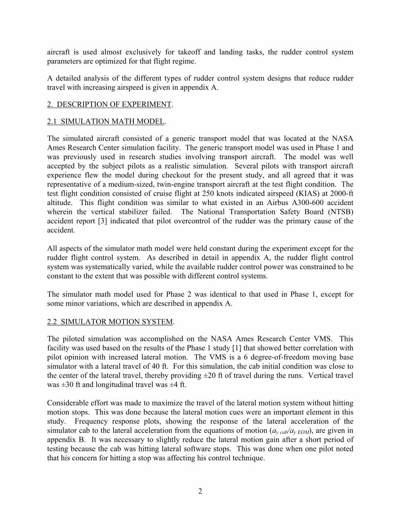
The loads on the vertical stabilizer result from a combination of sideslip and rudder deflection. Figure 11 shows that the force on the vertical stabilizer is maximized when sideslip and rudder deflection are of opposite sign. For sideslip and rudder deflection to be of opposite sign, the pilot must have applied rudder in a direction to reduce sideslip. This puts the rudder in the shaded red “overcontrol” region in figure 11.

17

β βV V

δr δr

REGION OF OVERCONTROLForce due to rudder deflection,F( r) adds to forcedue to sideslip, F( ).

and r have opposite sign (leads to large| - r|).

δβ

β δβ δ

Force due to rudder deflection,F( r) subtracts from force due to sideslip, F( ).

and r have the same sign (leads to reduced| - r|).

δβ

β δβ δ

Negative rudderdeflection

Positive sideslip

Airspeed VectorAirspeed Vector

Positive sideslip

Positive rudderdeflection

F( r)δF( r)δ

F( )β F( )β

Figure 11. Region of Overcontrol

When rudder is used to augment aileron (as was required to accomplish the task), the pilot intentionally sideslips in a direction to cause the effective dihedral (Lβ) to add to the rolling moment due to aileron. When this is done, rudder deflection and sideslip have the same sign and the force on the vertical stabilizer due to rudder deflection subtracts from the force due to sideslip. It is only when the pilot reverses the rudder in the presence of large sideslip that the forces are added, as defined by the shaded region in figure 11. Analysis of the simulation data indicated that significant rudder deflections into the overcontrol region occurred as a result of two distinct pilot techniques when regulating against large rolling disturbances. • Pilot Technique A. Pilot does not use rudder until full aileron deflection is applied, and

the aircraft is still rolling away from the applied aileron. At that point, a rudder input is made to augment the aileron. This tends to result in excursions into the overcontrol region because there is some sideslip due to the adverse yaw that develops with full aileron deflection. The avoidance of rudder to augment aileron until it is absolutely necessary is consistent with current training.

• Pilot Technique B. Pilot uses rudder continuously to augment roll control with aileron.

18

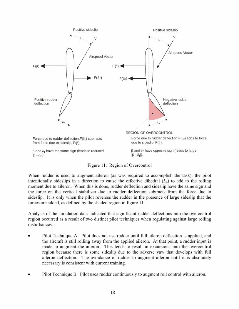
An example of technique A is shown in figure 12. Here, the pilot inputs full aileron to counter a large rolling gust with essentially no rudder input. The yaw damper cannot quite keep up with the large aileron input, resulting in a small positive sideslip (adverse yaw). When the pilot finally decides that rudder is necessary, he abruptly puts in full rudder control. The rudder enters the overcontrol region, resulting in a peak in the force on the vertical stabilizer. As long as the yaw damper minimizes the adverse yaw due to a full aileron input, the sideslip will remain small, and forces on the vertical stabilizer should not be excessive. Pilot technique B is shown in figure 13. The pilot is using rudder in a continuous manner. The sign of rudder and sideslip are the same, as expected when rudder is used to augment aileron. However, if the pilot gets out of phase with aileron or momentarily misapplies the rudder, the forces on the vertical stabilizer due to rudder and sideslip add. This occurs at 75.8 seconds, and a peak in the force on the vertical stabilizer is observed. This is similar to the scenario that resulted in failure of the vertical stabilizer in the NTSB report [3] (albeit, with a much greater magnitude of sideslip). The time histories in figure 13 are from the simulation run that produced the highest vertical stabilizer in Phase 2. While it is not the intent of this study to reconstruct the accident that led to failure of the vertical stabilizer reported in reference 3, it is illustrative to review the data from that accident in terms of the above discussion. The time histories in figure 14 were derived from the data in reference 5. These time histories indicate that the pilot was actively using rudder to augment aileron during the initial portion of the encounter (pilot technique B). This is evidenced by the fact that rudder was used to develop perverse yaw (sideslip has the same sign as rudder and in a direction to augment roll). Approximately 2.5 seconds into the encounter, the rudder is held against the right pedal stop, while the wheel is reversed to 20° left, followed by 50° right, and back to 40° left. This lack of correlation between aileron and rudder excited the Dutch roll mode, resulting in large sideslip angles. This was probably exacerbated by the fact that the yaw damper was only partially functional while the pilot held the pedal on the stop. The pilot then made a full rudder input from one stop to the other, resulting in maximum negative rudder in the presence of 10° of positive sideslip (i.e., full rudder input into the shaded overcontrol region in figure 11), which caused the vertical stabilizer to fail. This scenario is an extreme example of pilot technique B.

19

-100

0

100δ W

(%

)Cfg: 1, Run #: 915, Pilot #: 9

-100

0

100

δ P (

%)

δpMAX = 1.2 (in)

-50

0

50

p G (

deg/

sec)

,φ (

deg)

pG

φ

0

20

40

|Fv|

(10)

3 (lb

s)

δr-MAX = 9 (deg), βMAX = 4.4 (deg), |βmeas|Peak = 4.2 (deg), |Fv|Peak = 26082 (lbs)

-10

0

10

β (d

eg)

65 66 67 68 69 70 71 72 73 74 75-10

0

10

δ r (de

g)

Time (sec)

Figure 12. Example of Pilot Technique A

20

-100

0

100δ W

(%

)Cfg: 15, Run #: 719, Pilot: Kevin Greene

-100

0

100

δ P (

%)

δpMAX = 1.2 (in)

-50

0

50

p G (

deg/

sec)

,φ (

deg)

pG

φ

0

20

40

|Fv|

(10)

3 (lb

s)

δr-MAX = 9 (deg), βMAX = 4.4 (deg), |βmeas|Peak = 5.7 (deg), |Fv|Peak = 32166 (lbs)

-10

0

10

β (d

eg)

60 62 64 66 68 70 72 74 76 78 80-10

0

10

δ r (de

g)

Time (sec)

Figure 13. Example of Pilot Technique B

21

Figure 14. Time Histories Leading to Failure of Vertical Stabilizer

The FAA regulatory criteria that relate to vertical stabilizer structural integrity are specified in Title 14 Code of Federal Regulations (CFR) 25.351. The key elements of that requirement are as follows:

“(a) With the airplane in unaccelerated flight at zero yaw, it is assumed that the cockpit rudder control is suddenly displaced to the limit of travel.

- 80 - 60 - 40 - 20

0 20 40 60 80

0 2 4 6 8 10 12 14

Wheel (deg)

Time

- 15 - 10 - 5 0 5

10 15

0 2 4 6 8 10 12 14

Pedal Displacement

(deg)

Time

- 15 - 10 - 5 0 5

10 15

0 2 4 6 8 10 12 14

Rudder Displacement

(deg)

Time

- 15 - 10 - 5 0 5

10 15

0 2 4 6 8 10 12 14

Sideslip (deg)

Time

- 0.6 - 0.4 - 0.2

0 0.2 0.4

0 2 4 6 8 10 12 14

Lateral

Ver

tical

Sta

biliz

er S

truct

ural

Fai

lure

Load

Factor (g’s)

Time

22

(b)With the cockpit rudder control deflected so as always to maintain the maximum rudder deflection available, it is assumed that the airplane yaws to the overswing sideslip angle. (c) With the airplane yawed to the static equilibrium sideslip angle, it is assumed that the cockpit rudder control is held so as to achieve the maximum rudder deflection available. (d) With the airplane yawed to the static equilibrium sideslip angle of paragraph (c) of this section, it is assumed that the cockpit rudder control is suddenly returned to neutral.”

14 CFR 25.351 specifies that the airplane must be designed to withstand the loads (resulting from the above maneuvers) from the minimum control airspeed (VMC) to the maximum dive speed (VD). 14 CFR 25.351(d) is the most critical input because the forces due to sideslip are always higher than the force due to rudder (for example, see equation 4). The objective of this study was to identify characteristics of the rudder flight control system that make it more likely that rudder usage would result in forces higher than required by 14 CFR 25.351(d). If the force on the vertical stabilizer resulting from the maneuver specified by 14 CFR 25.351(d) is defined as Fβmax, then from equation 3

2

0max max( )

2CAS

Y ssS VF C

ββ

ρ= β (5)

If the rudder structure is designed in accordance with 14 CFR 25.351(d), forces exceeding Fβmax will result in exceedance of the limit load on the vertical stabilizer. This is expressed as a percentage over the limit load as follows.

3

max

1 100peakEF

FF

Fσ

β

⎛ ⎞Δ = −⎜ ⎟⎜ ⎟

⎝ ⎠ (6)

Where F3σ peak is defined as the largest expected force on the vertical stabilizer. If a vertical stabilizer structure is designed so that the design limit load is defined by Fβmax, then the ultimate load (1.5 times the limit load) would be defined when ΔFEF = 50%. Forces above Fβmax can only occur if the rudder enters the shaded overcontrol region in figure 11 in the presence of significant sideslip.

23

F3σ peak was calculated from the simulation data as follows: 1. Identify and store the peak (maximum) value of vertical stabilizer force ( peakF ) for a

group of runs, e.g., for all runs where Flim = 60 lb and δpedmax = 1.2 inches. 2. Calculate the average of peakF for all runs from step 1. 3. Calculate the standard deviation of peakF for all runs. 4. *

3 3 (peak avg peak peakF F std dev Fσ = + )

Appendix E shows that the peakF data from the simulation is well described by a normal distribution and, therefore, using the 3σ value is a reasonable estimate of the maximum force on the vertical stabilizer that would ever be encountered while accomplishing a task requiring use of rudder to augment aileron. The only way that the force on the vertical stabilizer can exceed Fβmax is for the pilot to make a rudder input into the overcontrol region when sideslip is large. The maximum achievable force that can be obtained from static equilibrium occurs by establishing the conditions specified by 14 CFR 25.351(c) (maximum steady sideslip) and suddenly reversing the rudder to the opposite stop (rather than centering the rudder as required by 14 CFR 25.351(d). An example of that maneuver is shown in figure 15, which shows the maximum steady sideslip to be 4.4 degrees. From equation 4, this results in Fβmax = 26,705 lb. The peak force due to a rudder reversal from maximum sideslip, shown in figure 15, is 40,000 lb. From equation 6

[ ]40,000 / 26,705 1 100 49.8%EFFΔ = − = This indicates that a stop-to-stop rudder reversal at maximum steady sideslip can result in reaching the ultimate load factor.

24

Ped

al D

efle

ctio

n (in

.)│ r

Figure 15. Rudder Reversal at Maximum Sideslip

4.3 RUDDER OVERCONTROL PARAMETER.

As discussed in section 4.2, large vertical stabilizer forces occur when the pilot makes a large rudder input in the presence of sideslip and the sign of rudder deflection is opposite the sign of sideslip. Stated mathematically, this occurs when the parameter rβ−δ takes on large values. A

generic plot of the effect on increasing rβ− δ on the force imposed on the vertical stabilizer is shown in figure 16.

│β

- δ

Side

slip

(deg

)Fo

rce

on V

ertic

alS

tabi

lizer

(lb)

Configuration 60-10-1: Maximum force = 60 lb, Breakout = 10 lb, Maximum pedal = 1.2 inches

25

δ rlim

β β

δ

= ss max Vary r

βss max

δδ

β

r = r Lim

Var

y

β δ- rMA

Fv -

For

ce o

n V

ertic

al S

tabi

lizer

Region ofSignificantOvercontrol

ROP > 0

ROP = 1.0

ROP < 0

CFR 25.351(d)criterion( r = 0 and = ss max)δ β β

CFR 25.351(a)criterion( r = rLim

and = 0)δ δ β

rβ− δ

Figure 16. Effect of rβ−δ on Vertical Stabilizer Force

The boundaries in figure 16 are based on steady-state conditions. The upper boundary is the vertical stabilizer force that results from a step rudder input in the presence of the maximum achievable steady-state sideslip (β = βss max). Higher values of sideslip can be achieved if rudder inputs are made to excite the Dutch roll mode. The lower boundary is the force resulting from varying sideslip in the presence of maximum rudder (δr lim). The curves intersect when rβ−δ is

at its maximum achievable value r MAβ− δ (defined when max lim and ss r rβ = β δ = δ and sign β ≠

sign δr). The possibility for high vertical stabilizer loads increases significantly as rβ− δ takes on values greater than δrlim (shown as the shaded region in figure 16). This is defined as the region of significant rudder overcontrol. The tendency for rudder reversals that result in excursions into the region of significant rudder overcontrol is quantified by positive values of the rudder overcontrol parameter (ROP).

lim lim3 3

lim max

r r rpeak peak

r r ssMA

ROP σ σβ − δ −δ β−δ −δ

= =β−δ −δ β

r (7)

ROP is normalized by the condition where sideslip and rudder are at their maximum achievable values without dynamic overshoot. This is done to minimize the effect of rudder control power so that ROP is primarily a measure of the tendency for rudder reversals into the significant overcontrol region in figure 16.

26

The following connections may be established between ROP and rudder overcontrol events: • ROP >0—The force on the vertical stabilizer is greater than can be achieved with rudder

alone (i.e., greater than specified by 14 CFR 25.351(b)). • ROP = 1—The maximum force that can be achieved at steady sideslip. Accomplished by

achieving the maximum steady sideslip with full rudder and rapidly reversing the rudder to the opposite limit.

• ROP >1—Forces exceed what can be achieved at steady sideslip—indicates rudder

reversal at sideslip greater than can be achieved in steady state (i.e., β >βss max).

3 r peakσβ − δ was calculated from the simulation data as follows:

1. Identify and store the peak (maximum) value of vertical stabilizer force ( )r peak

β−δ for a

group of runs, e.g., for all runs where Flim−60 lb and δpedmax = 1.2 inches. 2. Calculate the average r peak

β−δ for all runs from step 1.

3. Calculate the standard deviation of r peak

β−δ for all runs

4. ( )3

3* r r r peak−

peak avg peakstd dev

σβ − δ = β−δ + β δ

Appendix E shows that the r peak

β−δ data from the simulation is well described by a normal

distribution and, therefore, using the 3σ value is a reasonable estimate of the maximum expected value. The calculation of the standard deviation of rβ− δ is based on all configurations in the test matrix (figure 8). The calculation of a separate standard deviation for each configuration did not exhibit a consistent trend, indicating that the variability in the use of rudder was not configuration-dependent. It was, therefore, decided to calculate a single standard deviation for all 1014 runs. The intent of the rudder overcontrol criterion is to provide a metric to distinguish between rudder control systems that are prone to overcontrol from those that are not. Note, it is possible to experience rudder deflections in the region of overcontrol without exerting exceptional forces on the vertical stabilizer if sideslip is low when the rudder is over controlled (lower portion of shaded region in figure 16). Therefore, ROP can be quite large without experiencing excessive vertical stabilizer load. The basic concept of ROP is that values greater than zero indicate a tendency to overcontrol, and it is conceptually just a matter of time until such an excursion will occur in the presence of large sideslip (e.g., figure 14).

27

The current 14 CFR Part 25 351(d) criterion plots at a point on the upper boundary where steady sideslip is maximum and rudder deflection is zero, and the 14 CFR 25.351(a) criterion plots at a point on the lower boundary where rudder deflection is maximum and sideslip is zero. The data obtained from the baseline and YD B configurations in Phase 2 are plotted on figure 16 boundaries and shown in figure 17, where the peak force versus peak value of rβ− δ are plotted for each run.

5000

10000

15000

20000

25000

30000

35000

40000

45000

4 6 8 10 12 14

1.2 in2.4 in3.5 in

δr-LIM |β-δr|MA

βSS-MAX

CFR 14 25.351(d)Criterionδr = 0 deg

CFR 14 25.351(a)Criterionβ= 0 deg

│Fv│Peak (lb)

│β-δr│Peak (deg)

Figure 17. Effect of rβ−δ on Vertical Stabilizer Force—Phase 2 Baseline Configurations (δrlim = 9° and βssmax = 4.4°)

These data indicate that most runs did not exhibit significant overcontrol (ROP <0), and the runs where overcontrol did occur plotted near the lower boundary. This indicates that rudder overcontrol occurred mostly at low sideslip values, which implies that there was little tendency to excite the Dutch roll mode during the Phase 2 tests. Time histories for the run corresponding to the highest value of vertical stabilizer force plotted in figure 17 (approximately 32,000 lb) are shown in figure 13. The data for some runs fell below the lower boundary because the airspeed was slightly below the 250-kts target when the vertical stabilizer force peaked. 5. CRITERIA DEVELOPMENT.

The objective of this work is to develop proposed criteria and supporting data that allow the FAA to make recommendations regarding the design of rudder flight control systems that are resistant to pilot-induced overstressing of the vertical stabilizer in up-and-away flight.

28

5.1 TECHNICAL APPROACH.

The analysis discussed in this report shows that high vertical stabilizer loads result from a rudder reversal into the region of overcontrol at large sideslip values. The ROP was developed as a tool to analyze the data obtained in this experiment. As noted in figure 16, the tendency to overcontrol with rudder increases as ROP takes on values greater than zero. A successful criterion parameter will show good correlation with ROP, and thereby distinguish between configurations that are prone to overcontrol from those that are not. Note that ROP itself cannot be used as a criterion parameter because it requires a large amount of data, which is not practical for evaluating an actual rudder flight control system design. As shown in figures 16 and 17, it is possible to experience a range of forces on the vertical stabilizer for a given value of ROP, depending on sideslip. The approach taken here is that a good criterion will ensure that ROP is low so that it will be unlikely to encounter a rudder reversal at any value of sideslip, whether it was pilot-induced or a result of turbulence or a wake vortex encounter. The parameter has also been developed to analyze the simulation data. This parameter is a measure of the excess force imposed on the vertical stabilizer relative to the force required to meet 14 CFR 25.351(d). = 0 implies that the peak force on the vertical stabilizer is equal to the force that would occur for maximum steady sideslip with zero rudder, as specified by 14 CFR 24.351(d). This parameter is intended to put the simulation results in the proper context. Values of 50% or greater are considered to have the potential for structural failure of the vertical stabilizer. This is based on the argument that if the structure was designed so that the limit load just meets the 14 CFR 25.351(d) criterion, then the ultimate load would be 50% higher.

EFFΔ

EFFΔ

5.2 EFFECT OF PEDAL TRAVEL, LIMIT PEDAL FORCE, AND Fbo/Flim.

The basic hypothesis of the Phase 2 simulation test plan was that rudder overcontrol is strongly dependent on the highly nonlinear nature of the rudder pedal force deflection or load-feel curve due to large values of breakout. A simple measure of this nonlinearity is Fbo/Flim, the breakout force divided by the limit force (see section 3.1 for definitions of breakout and limit force). The results of the Phase 2 simulation in terms of Fbo/Flim and the value of ROP taken as an average across all pilots for each baseline configuration were plotted and are shown in figure 18. These results are based on using a standard deviation of 1.18° to calculate

3 r peakσβ − δ in

equation 7. As noted in section 4.3, the calculation of the standard deviation of rβ− δ is based on all runs for all configurations in the test matrix (figure 8).

29

0.20

0.40

0.60

0.80

0.00 0.20 0.40 0.60 0.80

Rud

der O

verc

ontr

ol P

aram

eter

, RO

P

Fbo/Flim

35-XX-1

35-XX-2

35-XX-3

60-XX-1

60-XX-2

60-XX-3

All Pilots: Std Dev |β-δr|Peak = 1.18 deg (N = 1014)

Figure 18. Rudder Overcontrol Parameter as a Function of Fbo/Flim for Baseline Configurations

Each configuration was run an average of 22 times with each pilot nominally evaluating three randomly inserted repeat runs for each configuration. The minimum number of runs for a given configuration was 20 and the maximum was 38. This was judged to be a significantly large sample to provide reliable trends.1 The most significant finding from the data in figure 18 is that the tendency to overcontrol with rudder is primarily dependent on rudder pedal travel. The 3.5-inch-long pedal throw configurations (circle symbols) were consistently and significantly less prone to overcontrol than the 1.2-inch short pedal throw configurations (diamond symbols). Other conclusions from the figure 18 data are: • The configurations with high limit force, long pedal throw, and Fbo/Flim between 0.25 and

0.42 (60-15-3 and 60-25-3) exhibited the lowest ROP values, indicating a strong resistance to rudder overcontrol.

• Increasing the pedal limit force did not significantly alleviate the tendency for

overcontrol for the short pedal throw configurations (compare the open and filled diamonds in figure 18).

1Early in the program, the configurations were evaluated three consecutive times before providing a rating. This was changed so that only one run was made before moving to the next configuration. When more than one run was made, only the first run was used in the data analysis.

30

• The ratio of Fbo/Flim had little effect on the tendency for overcontrol with the following exceptions.

- A significant decrease in ROP occurred when Fbo/Flim was set equal to 0.25 for

the short pedal throw configuration 60-15-1. This seemingly anomalous trend was noticed during the simulation and extra runs were made to determine if this effect was real. A total of 23 runs, with a standard deviation of 1.1o, suggest that this was not a random effect. This was the only case where a reduction in Fbo/Flim resulted in a large and beneficial effect on ROP (albeit, not as good as increasing the travel to 3.5 inches).

- Decreasing the breakout to 5 lb (Fbo/Flim ≈0.10) resulted in a noticeable increase

in ROP for some configurations. The pilots all complained of a “mushy feel” for this low value of breakout. This result suggests that there is a minimum value of breakout to ensure that ROP is minimized.

- A slight increase in ROP resulted from increasing Fbo/Flim to values greater than

0.42 for the long pedal throw (3.5 inches) configurations. A plot of the results in terms of pedal travel is shown by plotting ROP for each pedal displacement/force versus pedal travel2 (figure 19). The symbols represent the averaged value, the thick vertical lines represent the standard deviation of the averaged values, and the end points represent the maximum and minimum values of ROP.

-0.4-0.2

00.20.40.60.8

11.21.41.6

0 1 2 3 4

Rud

der

Ove

rcon

trol

Par

amet

er -

RO

P

Maximum Pedal Displacement, δp-lim (in)

35-XX-X

60-XX-X

All Pilots: Std Dev |β-δr|Peak = 1.18 deg (N = 1014)

Figure 19. Plot of ROP vs Pedal Travel for Baseline Configurations

2ROP is based on the value of r peak

β−δ averaged across all pilots and Fbo/Flim for each pedal displacement/force

configuration.

31

This data shows that increasing pedal travel is a considerably more effective way to reduce the tendency for rudder overcontrol than increasing pedal force. The large variation between the maximum and minimum values of ROP for a given pedal displacement/force is a result of different pilot techniques. Some pilots were considerably more aggressive than others. The excess vertical stabilizer force as a function of maximum pedal throw is shown by plotting ΔFEF obtained by averaging Fpeak across all pilots and configurations at each of the three tested pedal displacements (figure 20).

0

5

10

15

20

25

0 1 2 3 4

ΔFE

F(%

)

Maximum Pedal Displacement, δP-LIM (in)

35-XX-X

60-XX-X

Figure 20. Excess Vertical Stabilizer Force vs Pedal Throw

These data indicate that ΔFEF exhibits the same trend as ROP in that the short pedal throw configurations are more prone to high vertical stabilizer loads, and pedal force plays a less significant role. This data shows that the worst-case configuration (short pedal throw and low force) exceeded the 14 CFR 25.351(d) criterion, on average, by 21% and the best configuration (long pedal throw and high force) exceeded the criterion by 8%. That is, all the configurations exceeded the criterion limit, but the short pedal throw configurations were prone to a significantly higher exceedance. To put these results in context, a full rudder reversal from a maximum steady sideslip condition would result in ΔFEF = 50%.3

3This result is obtained from the calculation shown in equations 5 and 6.

32

The A300-600 vertical stabilizer failed with β = 10°, δr = -11°, and airspeed = 250 kts4. Substituting these values into the estimated vertical stabilizer force (equation 4) results in a force on the vertical stabilizer of 80,327 lb. The 14 CFR 25.351(d) limit (Fβmax) is calculated from equation 4 by setting β = 4.4°, δr = 0°, and airspeed = 250 kts, resulting in a value of 26,705 lb. Therefore, the estimated value of ΔFEF at the point of failure was 200%. This is an order of magnitude greater than what was experienced in the Phase 1 or Phase 2 VMS simulations. As will be discussed in section 5.5, the less than expected vertical stabilizer loads encountered in the simulation were due to sideslip excursions that were much less than in the accident scenario. 5.3 LINEARITY INDEX PARAMETER.

The linearity index (LI) was proposed in references 6 and 7 as a measure of tendency to overcontrol with rudder. LI was calculated for all the baseline configurations, as shown in appendix F. Appendix F also shows that LI ≈ 1 – Fbo/Flim for all the configurations tested in this simulation. ROP was correlated with LI, as shown in figure 21.

0.20

0.40

0.60

0.80

0.25 0.45 0.65 0.85

Rud

der O

verc

ontr

ol P

aram

eter

, RO

P

Linearity Index, LI

35-XX-1

35-XX-2

35-XX-3

60-XX-1

60-XX-2

60-XX-3

All Pilots: Std Dev |β-δr|Peak = 1.18 deg (N = 1014)

Figure 21. Correlation of ROP With LI

As expected, the correlation of ROP with LI indicates the same trends as the correlation with Fbo/Flim in figure 19, albeit flipped horizontally because LI ≈ 1 – Fbo/Flim. In conclusion, the LI describes the same phenomena as Fbo/Flim, and the parameters can be used interchangeably for configurations with similar rudder pedal load-feel characteristics with those 4It is unknown why the flight data recorder showed a rudder deflection of -11° when the rudder should have been mechanically limited to 9° based on the data in reference 3.

33

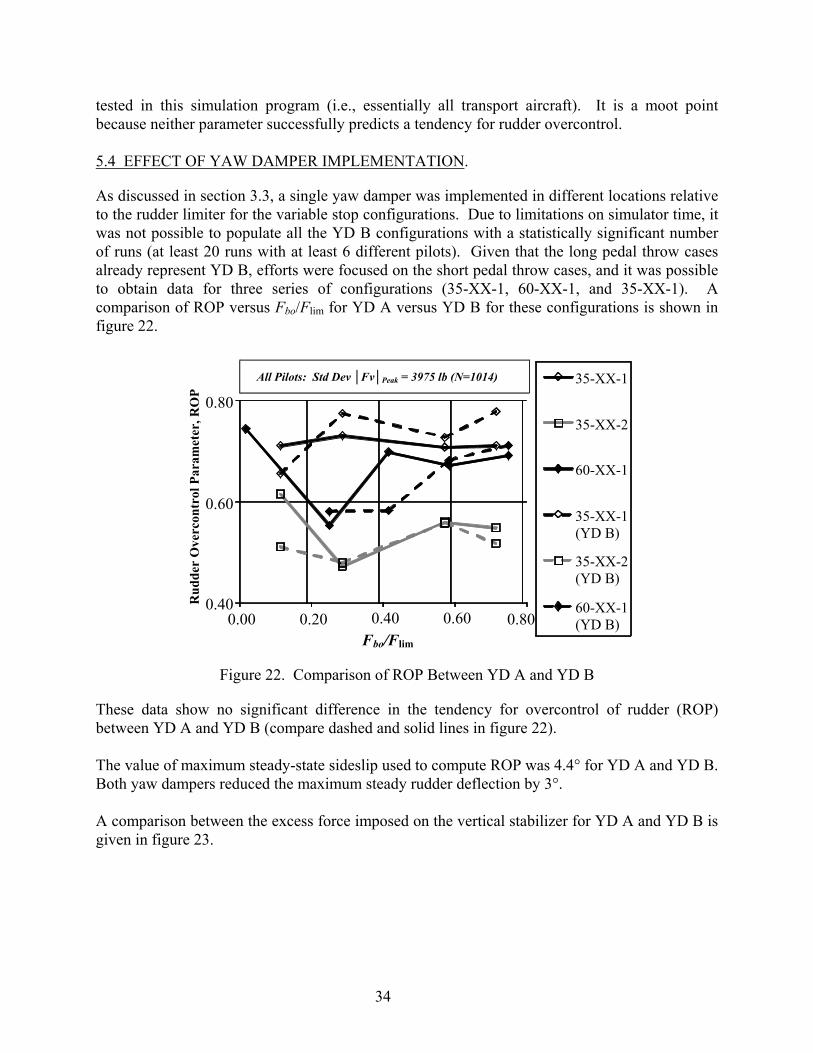
tested in this simulation program (i.e., essentially all transport aircraft). It is a moot point because neither parameter successfully predicts a tendency for rudder overcontrol. 5.4 EFFECT OF YAW DAMPER IMPLEMENTATION.

As discussed in section 3.3, a single yaw damper was implemented in different locations relative to the rudder limiter for the variable stop configurations. Due to limitations on simulator time, it was not possible to populate all the YD B configurations with a statistically significant number of runs (at least 20 runs with at least 6 different pilots). Given that the long pedal throw cases already represent YD B, efforts were focused on the short pedal throw cases, and it was possible to obtain data for three series of configurations (35-XX-1, 60-XX-1, and 35-XX-1). A comparison of ROP versus Fbo/Flim for YD A versus YD B for these configurations is shown in figure 22.

0.8060-XX-1 (YD B)

35-XX-2 (YD B)

35-XX-1 (YD B)

60-XX-1

35-XX-2

35-XX-1

0.600.40

0.80

0.60

0.40 0.00 0.20

All Pilots: Std Dev │Fv│Peak = 3975 lb (N=1014)

Rud

der

Ove

rcon

trol

Par

amet

er, R

OP

Fbo/Flim

Figure 22. Comparison of ROP Between YD A and YD B

These data show no significant difference in the tendency for overcontrol of rudder (ROP) between YD A and YD B (compare dashed and solid lines in figure 22). The value of maximum steady-state sideslip used to compute ROP was 4.4° for YD A and YD B. Both yaw dampers reduced the maximum steady rudder deflection by 3°. A comparison between the excess force imposed on the vertical stabilizer for YD A and YD B is given in figure 23.

34

25

1.5 2 2.5 3 3.5 4Maximum Pedal Displacement, δp-lim (in.)

35-XX-X (YD A)

60-XX-X (YD A) 35-XX-X (YD B) 60-XX-X (YD B)

1

20

15 ΔFEF

(%) 10

5

0

Figure 23. Comparison of Excess Force on Vertical Stabilizer Between YD A and YD B

These data indicate that there is no significant difference in the force imposed on the vertical stabilizer between YD A and YD B. 5.5 LARGE SIDESLIP AS A CONTRIBUTING FACTOR.

As shown in figure 15, the maximum achievable steady sideslip for the baseline configurations was 4.4°, and a rapid rudder reversal at that sideslip angle resulted in a vertical stabilizer load of approximately 40,000 lb. This is far below the estimated 80,327-lb load that resulted in the in-flight structural failure shown in figure 14. The large discrepancy between this event and the simulation results can be explained primarily by the fact that sideslip was never increased to the level experienced by the accident aircraft (10°). The peak sideslip5 angles that occurred during the simulation for the baseline cases are shown in figure 24. The symbols in figure 24 indicate the average peak sideslip, the ends of the thick vertical bars indicate the 1 σ variations in peak sideslip, and the T-ends indicate the maximum and minimum values of sideslip achieved for all baseline configuration runs. The short pedal throw configurations tended to produce larger values of sideslip, indicating more Dutch roll excitation. The maximum steady-state sideslip that could be achieved with maximum rudder deflection for the baseline configurations was 4.4°. The maximum sideslip achieved in the simulation was 5.8°, which is 1.4° more than the steady-state value.

5The peak sideslip is defined as the maximum sideslip that occurred during a 63-second simulation run.

35

2

2.5

3

3.5

4

4.5

5

5.5

6

0 1 2 3 4

|ß|Peak(deg)

Maximum Pedal Displacement, dP-LIM (in)

35-XX-X

60-XX-X

Figure 24. Maximum Sideslip for Baseline Configurations

The maximum sideslip achieved during the simulation was only slightly more than half that achieved in the accident scenario (10°) shown in figure 14. From equation 4, the maximum force that could have been exerted on the vertical stabilizer had the pilot reversed the rudder at the worst-case sideslip value of 5.8° would have been 51,267 lb (maximum rudder = 9°), as shown by the following calculation.

( ) [ ]2 20.034 0.01 0.034(5.8 0.01( 9) (250*1.69) 51, 267 lbv r CASF V= − β+ δ = − + − = This is compared to the force of 40,000 lb that can be achieved for a maximum rudder reversal at the maximum steady sideslip angle of 4.4° (see figure 15). Note that the force on the vertical stabilizer increases by approximately 6000 lb for every degree of sideslip. These results suggest that a tendency towards large sideslip angles plays a significant role in achieving large aerodynamic loads on the vertical stabilizer. Such a tendency would most likely result from a combination of degraded yaw damper performance and increased rudder control power. The effect of the yaw damper implementation (YD A and YD B) and the rudder control power on the peak sideslip angle achieved in the simulation is shown in figure 25. These data show that the effect of locating the yaw damper before or after the limiter (YD A and YD B, respectively) had only a minor effect on the peak sideslip angle. Increasing the rudder authority from 9° to 12° resulted in slightly increased sideslip excursions.

36

1

2

3

4

5

6

7

8

9

ßPeak(deg)

YDA, dr-LIM = 9YDA, dr-LIM = 12YDB, dr-LIM = 9YDB, dr-LIM = 12

Figure 25. Effect of Yaw Damper A vs Yaw Damper B on Maximum Sideslip

These results call into question how the sideslip angle on the A300-600 accident aircraft became so large (10° at point of failure, see figure 14). Even with rudder control power increased by 33%, the largest sideslip angle achieved during the simulation was 8.3°. A cursory MATLAB® Simulink® analysis was performed to investigate the effect of degrading the yaw damper and increasing rudder control power on peak sideslip to provide some insight into how very large values of sideslip could be achieved in a transport aircraft. The desktop simulation consisted of a linear model of the Convair 880, as described in appendix G6. Yaw Damper A was implemented into the Convair 880 model. The rudder and aileron inputs from the AA Flight 587 A300-600 accident were used to drive the model. The time histories of the response with a fully functioning (albeit saturated) yaw damper are shown in figure 26. These data indicate that the Convair 880 model achieved a peak sideslip angle of 5° (half that exhibited by the A300-600), similar to what was observed for the baseline cases in the simulation. One significant difference between the time histories of the rudder response of the Convair 880 in figure 26 and the A300-600 (figure 14) is that the maximum rudder deflections are less for the Convair 880 (which used YD A). According to information published in reference 3, the rudder deflection for the A300-600 was mechanically limited to approximately 9° at 250-kts airspeed where the vertical stabilizer failed. Figure 14 shows that the rudder achieved values as high as 11°. It is unknown why the rudder reached deflections beyond its mechanical limit.

6This model was used because linear aerodynamic data was readily available from reference 8.

37

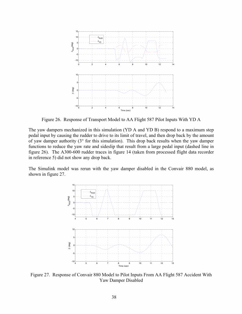
0 2 4 6 8 10 12 14

-10

-5

0

5

10

15

δ RU

D(d

eg)

δRUD

δYD

0 2 4 6 8 10 12 14-10

-5

0

5

10β

(deg

)

Time (sec)

Figure 26. Response of Transport Model to AA Flight 587 Pilot Inputs With YD A

The yaw dampers mechanized in this simulation (YD A and YD B) respond to a maximum step pedal input by causing the rudder to drive to its limit of travel, and then drop back by the amount of yaw damper authority (3° for this simulation). This drop back results when the yaw damper functions to reduce the yaw rate and sideslip that result from a large pedal input (dashed line in figure 26). The A300-600 rudder traces in figure 14 (taken from processed flight data recorder in reference 5) did not show any drop back. The Simulink model was rerun with the yaw damper disabled in the Convair 880 model, as shown in figure 27.

4 5 6 7 8 9 10 11 12 13

-10

-5

0

5

10

15

δ RU

D(d

eg)

δRUD

δYD

4 5 6 7 8 9 10 11 12 13-10

-5

0

5

10

β (d

eg)

Time (sec)

Figure 27. Response of Convair 880 Model to Pilot Inputs From AA Flight 587 Accident With Yaw Damper Disabled

38

Disabling the yaw damper approximates the effect of increasing the pedal-to-rudder gearing to allow the pilot to command a rudder deflection that is well over the rudder limit, as described in section 3.3.1. This caused the peak sideslip to increase 40% from 5° to approximately 7°. The rudder control power of the Convair 880 (Nδr) was increased by 50% to achieve 10° of sideslip with the yaw damper inoperative, as shown in figure 28.

4 5 6 7 8 9 10 11 12 13

-10

-5

0

5

10

15δ R

UD

(deg

)

δRUD

δYD

4 5 6 7 8 9 10 11 12 13-100

-50

0

50

100

δ WH

EE

L(deg

)

4 5 6 7 8 9 10 11 12 13-20

0

20

40

60

φ(de

g)

4 5 6 7 8 9 10 11 12 13-10

-5

0

5

10

β (d

eg)

CV880M

A300-600

4 5 6 7 8 9 10 11 12 13-0.5

0

0.5

a y-C

G (

gs)

Figure 28. Response of Convair 880 Model and A300-600 to Pilot Inputs From AA Flight 587 Accident With the Yaw Damper Disabled and 50% Increase in Rudder Control Power

The time history of the sideslip angle from the in-flight structural failure scenario (from figure 14) is also shown for comparison. The questions raised by this analysis were: • What design feature(s) would cause a saturated yaw damper to not deflect the rudder in a

direction to reduce yaw rate and sideslip? One example is described in section 3.3.1. • What design feature would cause the rudder to deflect to 11° when the mechanical limiter

is set at 9°? • What is a reasonable upper limit of rudder control power for transport aircraft?

39

The data discussed in section 5.8 indicates that ROP was significantly reduced when rudder control power was increased in this simulation, most likely because less rudder was required to provide the desired augmentation of aileron. This would not be the case if the effective dihedral is reduced (low Lβ), thereby requiring the pilot to use more rudder to augment aileron. In summary, a combination of high ROP, high control power, low effective dihedral, and a yaw damper that does not reduce the maximum rudder deflection when saturated, are all contributing factors that lead to large sideslip angles. 5.6 EFFECT OF HOLDBACK.

Physically, the holdback force is the force that exists when returning the pedals to neutral, just prior to the pedals being centered. The value of holdback was set to 2 lb for most of the test matrix to allow the maximum variation in Fbo/Flim (see section 3.2). The Lee, et al., rudder study [4] showed that values of holdback between 0 and 8 lb were acceptable. A brief study of the effect of holdback was conducted with four of the subject pilots. This consisted of conducting runs with holdbacks of 2 and 8 lb (configurations 35-25-1 and 36-25-1-HB) presented in the blind, and asking the pilots to describe any differences in rudder pedal characteristics. Excerpts of pilot commentary are given below. • Pilot 1—“Pedals felt the same” • Pilot 6 first look—“Could not tell the difference” • Pilot 6 second look—“Can feel better return but it would be easy to miss it. Does not

affect the way I fly or the ratings.” • Pilot 11—“Like this one best (the configuration with higher holdback) but the difference

is minor.” • Pilot 12—“Cannot tell one from the other” The values of r peak

β−δ were noted for each of the runs, and no consistent differences were

observed for the different values of holdback. These results confirm that holdback is not a factor for rudder overcontrol as long as it is kept within the values recommended in reference 4. 5.7 PILOT TECHNIQUE AND SUBJECTIVE RATINGS.

Two distinct types of pilot technique were observed during the simulation—those that did not use rudder until absolutely necessary (technique A) and those that used rudder continuously (technique B). It was also noted that some pilots used techniques A and B. In those cases, the

40

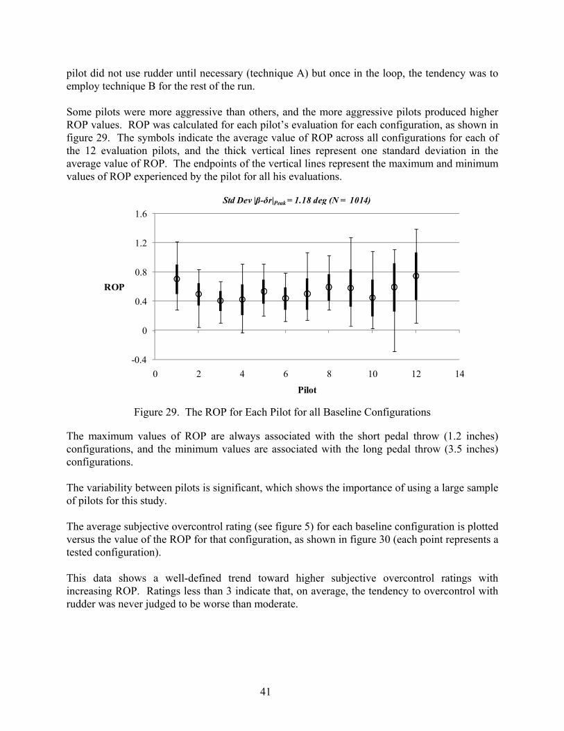
pilot did not use rudder until necessary (technique A) but once in the loop, the tendency was to employ technique B for the rest of the run. Some pilots were more aggressive than others, and the more aggressive pilots produced higher ROP values. ROP was calculated for each pilot’s evaluation for each configuration, as shown in figure 29. The symbols indicate the average value of ROP across all configurations for each of the 12 evaluation pilots, and the thick vertical lines represent one standard deviation in the average value of ROP. The endpoints of the vertical lines represent the maximum and minimum values of ROP experienced by the pilot for all his evaluations.

-0.4

0

0.4

0.8

1.2

1.6

0 2 4 6 8 10 12 14

ROP

Pilot

Std Dev |β-δr|Peak = 1.18 deg (N = 1014)

Figure 29. The ROP for Each Pilot for all Baseline Configurations

The maximum values of ROP are always associated with the short pedal throw (1.2 inches) configurations, and the minimum values are associated with the long pedal throw (3.5 inches) configurations. The variability between pilots is significant, which shows the importance of using a large sample of pilots for this study. The average subjective overcontrol rating (see figure 5) for each baseline configuration is plotted versus the value of the ROP for that configuration, as shown in figure 30 (each point represents a tested configuration). This data shows a well-defined trend toward higher subjective overcontrol ratings with increasing ROP. Ratings less than 3 indicate that, on average, the tendency to overcontrol with rudder was never judged to be worse than moderate.

41

1.0

1.5

2.0

2.5

3.0

0.2 0.3 0.4 0.5 0.6 0.7 0.8

Ave

rage

Ove

rcon

trol

Rat

ing

Rudder Overcontrol Parameter - ROP

Figure 30. Average Overcontrol Rating vs Average ROP for Each Baseline Configuration

The average overcontrol rating is plotted versus the average value of F3σ peak for each baseline configuration in figure 31 (note, F3σ peak is the largest expected force on the vertical stabilizer and is discussed in section 4.2.)

1.0

1.5

2.0

2.5

3.0

28000 30000 32000 34000

Ave

rage

Ove

rcon

trol

Rat

ing

Average F3σ-Peak (lbs)

Figure 31. Average Overcontrol Rating vs Average F3σ peak

As expected, the forces imposed on the vertical stabilizer tend to increase in proportion to the increase in overcontrol rating. The average HQR for each configuration is plotted versus the ROP, as shown in figure 32.

42

1

2

3

4

5

6

7

0.2 0.3 0.4 0.5 0.6 0.7 0.8

Ave

rage

HQ

R

Rudder Overcontrol Parameter - ROP

Figure 32. Average HQR vs Average ROP for Each Tested Configuration

These data indicate a weak trend showing increasing HQR with increasing values of ROP. There was considerable pilot commentary and discussion during the simulation regarding the assignment of subjective ratings. Most pilots agreed that because the task involved a semi out-of-control situation, it was difficult to separate the effect of rudder usage when assigning an HQR. Likewise, the overcontrol rating was found to be difficult to assign because most pilots could not decide exactly what constituted overcontrol. Attempts to define rudder overcontrol in terms of something that a pilot can identify were not successful. The rudder overcontrol parameters defined in section 4.2 are couched in terms of variables that are not obvious to the pilot (e.g., rβ−δ ). This suggests that there are only a few cues in the directional axis to warn the pilot of a potentially catastrophic failure, which is a significant consideration in the development of an overcontrol criterion. That is, the criterion cannot depend on pilot cueing in a similar manner to the stick force per g criterion in the longitudinal axis. 5.8 CONTROL POWER.

The effect of increased control power was investigated by increasing the rudder authority from 9° to 12° for some runs (configurations 40 through 51 in figure 8). The effect of increased control power on excess force on the vertical stabilizer (equation 6) and the rudder overcontrol parameter is shown in figure 33.

43

: 3975 ( 1014)

1.18 ( 1014)peak

peak

All Pilots Std Dev Fv lb N

Std Dev N

= =

β−δ = ° =

30.0

20.0

10.0

ΔFE 0.0 (%)

- 10.0

- 20.0 δrlim = 9°

- 30.0 δrlim = 12° - 40.0

- 0.60 - 0.40 - 0.20 0.00 0.20 0.40 0.60 0.80 1.00Rudder Overcontrol Parameter - ROP

Figure 33. Effect of Rudder Control Power

These results indicate that there is less tendency for overcontrol and, therefore, lower excess force on the vertical stabilizer for larger values of rudder control power. This is due to two factors: • The 14 CFR 25.351(d) criterion force (Fβmax) is higher (see section 4.2) because larger

steady-state sideslip angles can be achieved. • The pilots were able to achieve the desired effect of augmenting aileron with less rudder

input. These results should not be interpreted to mean that increased rudder control power is desirable, because the increase in Fβmax that goes with increased authority translates into a requirement for increased structural strength and, therefore, increased weight. Also, there is a tendency to incur larger values of sideslip with higher rudder control power, as shown in figure 25. 6. SIMULATOR MOTION EFFECTS.

As noted in section 2.2, a short exercise was done at the end of the simulation to investigate the use of a higher lateral motion gain (Gyf was increased from the nominal value of 0.4 to 0.6). Four of the pilots evaluated both short and long pedal throw configurations (35-25-1 and 60-15-3, respectively). The excerpted pilot comments were as follows. • Pilot 2—“Can definitely feel more lateral acceleration cues with increased motion gain,

especially at high frequency. I doubt that it has an effect on my rudder technique. If

44

anything I may tend to be less aggressive with rudder with the higher motion gain because the effect of a rudder input is felt immediately in the seat of the pants.”

• Pilot 6—“Concerned with hitting the wall with the higher motion gain – what we are

using is good enough. A little more kick in the seat of the pants. I m putting in the same pedal inputs as I use with the lower motion gain and see no effect on rating. I forgot the change 2/3 of the way through the run.”

• Pilot 11—“I am more cautious with rudder with the higher motion gains with the short

throw configuration. The motion gain has less effect on my rudder behavior for the long pedal throw configurations.”

• Pilot 12—“I can definitely feel the increased lateral motion. It provides better situational

awareness and feels more realistic.” The values of r peak

β−δ were noted for each run with the higher motion gain and the results

were unremarkable (i.e., consistent with values obtained with the lower motion gain). Pilot 11 was especially concerned with lateral motion and made numerous comments regarding the lack of lateral acceleration cues. The pilot felt that the higher motion gain afforded with Gyf = 0.6 would provide better results if the motion stop problem could be solved. One possible approach would be to test the higher motion gain by tailoring the disturbance input so most of the disturbances in a given run come from one direction. This would make it possible to set the initial condition of the simulator cab near one end of the lateral travel. Several such disturbance inputs would have to be provided so that the cab initial condition could be randomly biased to a point near the right and left ends of the 40-ft VMS travel. This approach should be investigated in Phase 3. It is recommended to verify the primary results of Phase 2 with increased motion before proceeding with Phase 3. This could be done by testing three values of Fbo/Flim for the short pedal throw configuration and two values of pedal travel (1.2 and 3.5 inches) at a nominal value of Fbo/Flim. 7. SUMMARY OF RESULTS.

The results of the Phase 2 simulation and data analysis are summarized as follows. • Very high vertical stabilizer forces result from rudder overcontrol in the presence of a

large sideslip angle.

- Rudder overcontrol is most likely with short pedal throw designs (1.2 inches of travel) than with long pedal throw designs (3.5 inches).

- Large sideslip angles depend on the details of the yaw damper functionality when

the yaw damper is saturated, rudder control power, and effective dihedral.

45

- Slightly larger sideslip excursions are more likely with short pedal throw designs than with long pedal throw designs.

• Increasing the maximum pedal force did not (noticeably) reduce the tendency for rudder

overcontrol for short pedal throw designs. • Long pedal throw in combination with higher maximum pedal force was shown to be an

effective way to minimize the probability of rudder overcontrol and to minimize sideslip excursions.

• The forces imposed on the vertical stabilizer were not large enough to cause structural

failure based on 14 CFR 25.351(d) criterion (stated mathematically is ΔFEF ≥50%). Most likely, this was because of the yaw damper, rudder control power, and effective dihedral used for the aircraft model in this simulation.

• The location of the yaw damper relative to the rudder limiter did not significantly affect

- the tendency for overcontrol of rudder. - the peak values of sideslip. - the forces imposed on the vertical stabilizer.

• Criteria to limit the possibility of overstressing the vertical stabilizer must include

- lower limits on the maximum pedal travel. - specifications on the functionality of the yaw damper in the presence of maximum

pedal displacements.

- consideration of rudder control power and effective dihedral. Other findings from the simulation were as follows: • The ROP was a good predictor of high forces on the vertical stabilizer for a given yaw

damper, rudder control power, and effective dihedral. • Parameters that attempt to quantify the pedal load-feel curve nonlinearity, such as

Fbo/Flim or the LI, are not effective in predicting the tendency for rudder overcontrol, with a few minor exceptions:

- For the 1.2-inch pedal throw configurations, using Fbo/Flim = 0.25 minimized the

tendency for overcontrol. However, this was not nearly as effective as increasing the pedal throw to 3.5 inches.

- For the 3.5-inch pedal throw configurations, the optimal range of Fbo/Flim was

between 0.25 and 0.42.

46

• Pilot technique varied significantly between pilots. Some pilots were more prone to overcontrol than others.

• Very low values of breakout, on the order of 5 lb, in the rudder feel system resulted in

degraded pilot opinion due to a “mushy feel.” Low breakout also increased the tendency for rudder overcontrol, especially for short pedal throw configurations.

8. CONCLUSIONS.

Factors that lead to a tendency to overstress the vertical stabilizer were identified as short pedal throw limits (less than approximately 3 inches), in combination with a yaw damper that becomes dysfunctional when saturated, and high rudder control power and low effective dihedral. Further study is needed to quantify the effects of yaw damper, rudder control power, and effective dihedral. The use of high pedal force gradients is only effective for long pedal throw designs where the pedal throw is approximately 3.5 inches or greater. Nonlinearities in the load-feel curve are not a significant factor for rudder overcontrol. 9. RECOMMENDATIONS.

Short pedal throw was identified as a primary contributor to rudder overcontrol. However, the tendency to overstress the vertical stabilizer also requires large sideslip angles. It is recommended that the Phase 3 study focus on factors that lead to large sideslip angles when augmenting aileron with rudder, such as • a yaw damper that becomes dysfunctional in terms of reducing rudder travel in the

presence of maximum or near-maximum pedal deflection. • high rudder control power in combination with low effective dihedral. A subset of runs should be included in Phase 3 to check the effect of increased motion. Bias the initial condition of the simulator cab and disturbance inputs so that the simulator does not hit lateral stops with increased motion. 10. REFERENCES. 1. Hoh, R.H., Nicoll, T.K., and Desrochers, P., “Piloted Simulation Study to Develop

Transport Aircraft Rudder Control System Requirements, Phase 1: Determine Simulator Motion Requirements and Initial Results,” FAA report DOT/FAA/AR-09/5, March 2009.

2. Hoh, R.H., “Simulation Test Plan to Develop Transport Aircraft Rudder Control System Requirements-Phase 2—Criteria Development,” HAI Technical Report 1137-2, July 31, 2006.

47

48

3. Anon, “In-Flight Separation of Vertical Stabilizer American Airlines Flight 587 Airbus Industrie A300-605R,” N14053 Belle Harbor, New York, November 12, 2001, NTSB/AAR-0404, PB2004-910404, Notation 7439B, October 12, 2004.

4. Lee, B., et al., “Effect of Pedal Feel System Characteristics on Aircraft HQ,” Proceedings of AIAA Atmospheric Flight Mechanics Conference, San Francisco, California, AIAA 2005-6034, 15-18 August 2005.

5. Callaghan, J.O., “Flight Control and Wake Turbulence Effects on American Airlines Flight 587,” Proceedings of AIAA Modeling and Simulation Technologies Conference, San Francisco, California, AIAA 2005-6110, 15-18 August 2005.

6. Hess, R.A., “Rudder Control Strategies and Force/Feel System Designs in Transport Aircraft,” Journal of Guidance, Control, and Dynamics, Vol. 28, Number 6, pp. 1251-1262, December 2005.

7. Hess, R.A., “Preliminary Assessment of Design Metrics for Transport Aircraft Rudder Control Systems,” A Presentation at NASA Langley.

8. Hefley, R.K. and Jewell, Wayne F., “Aircraft Handling Qualities Data,” STI Technical Report 1004-1, May 1972.

APPENDIX A—RUDDER FLIGHT CONTROL SYSTEMS

Generic versions of the three types of rudder flight control systems are discussed in this appendix. These are the same models that were used in Phase 1, except the cable stretch was assumed to be zero. This was done so the rudder control power was the same for the low and high values of rudder pedal force. Another deviation from Phase 1 was the maximum rudder and pedal deflections were not allowed to vary with airspeed. This was done to ensure that rudder control power did not vary if the pilot deviated from the target airspeed of 250 kts. As in Phase 1, the effects of structural compliance were not simulated. If the pilot applied a force of approximately 50 lb to the pedal on a typical transport rudder flight control system, structural compliance accounted for approximately 2% of the total pedal travel, which was determined to be insignificant for the purpose of this experiment. A.1 VARIABLE GEARING. The variable gearing design was used to simulate the long pedal throw designs. It is the only practical implementation for systems with long pedal throw. A generic variable gearing system is shown in figure A-1.

Fp

Load-feelSpring

RatioChanger

Ffsδp

δp

δpe

δpδp.

δp.

PilotInput

Kpe

d

Kped

Vcas

Pedal Stops+ 4 inches

Kvf

Kcs

1Fcf

viscousfriction

Coulombfriction

control loaderactuator

cable stretchcoefficient

δ r

Rudder Limiter

Rudderdeflection - deg

trim

+- Fbofs (breakoutof feel spring)

+

+ +-

+

-

pedal toruddergearing

Fcom

(Ffs + Fbofs)

(Ffs + Fbofs)

-

--

= +−30δ oLIMr

Kbofs

Kbofs = 200 lb/in

δr YD

δr Pilotδrcom

+- YDLIM

+

Yaw dampercommand to rudder

+

δbo = Kcs x Fbofs

Ffs

δp

Load Feel Spring with Breakout (All Rudder Systems)

Figure A-1. Generic Variable Gearing Rudder System

A-1

The force command to the control loader actuator (Fcom) is the sum of the viscous friction, Coulomb friction, load-feel spring, and breakout of the load-feel spring. Pedal motion occurs when the pilot force is not equal to Fcom. The pedal stops are achieved within the control loaders by increasing the spring force to a very large value. This is constant for the variable gearing system, but it is a calculated variable in the variable stop and force limit systems. Because Kbofs is a large number (100 lb/in), the feel spring breakout is a constant (Fbofs) for pedal deflections above approximately 0.10 to 0.20 inch (Fbofs/Kbofs) and has the sign of the pedal deflection. Variable gearing systems reduce the rudder control gearing (Kped = ratio of rudder travel-to-pedal travel) as a function of airspeed or dynamic pressure. As a result, the total pedal travel does not change, but the gradient of rudder surface deflection-to-pedal travel decreases as airspeed increases. Note, the rudder is not mechanically limited; its maximum travel being “limited” solely by the reduced gearing between pedal and rudder. The variable gearing is usually accomplished by means of a mechanical ratio changer (e.g., a variable lever arm). Since the yaw damper is always in series with the pedals (i.e., yaw damper does not cause pedals to move), the yaw damper servo effectively sums with the output of the ratio changer. As a consequence of this, the sum of the yaw damper input and pilot pedal motion can cause the rudder to momentarily exceed its theoretical limit. The advantage of this is that the yaw damper continues to perform its function regardless of the magnitude of the pilot input. The disadvantage of such a system is that a hardover failure could cause the rudder to move full travel (30°) at any airspeed. As noted in section 1.6.2.2 of reference A-1, the motivation for Airbus to change from a variable gearing system in the A300B2/B4 to a variable stop system in the A300-600 was that “it was less complex and had less severe failure modes.” The rudder pedal limits for the variable gearing system are fixed at ±3.5 inches. Rudder limiting is achieved by reducing Kped as a function of airspeed, as shown in figure A-3. The schedule of Kped versus calibrated airspeed is made such that the rudder deflection at full pedal is identical to the variable stop system at full pedal, at the same calibrated airspeed. The difference between the systems for this experiment is the full pedal for the variable gearing system is 3.5 inches and 1.2 inches for the variable stop and force limit systems. The variation of maximum rudder deflection as a function of airspeed is typically inversely proportional to the square of calibrated airspeed, i.e., dynamic pressure. The generic curve in figure A-2 reflects this relationship with minor adjustments based on a review of available data for (Douglas/Boeing and Airbus).

A-2

Rudder - deg

0

5

10

15

20

25

30

120 140 160 180 200 220 240 260 280 300 320

Calibrated Airspeed - kts

Max

imum

Rud

der D

efle

ctio

n - d

eg

Figure A-2. Limit on Rudder Travel as a Function of Calibrated Airspeed—Variable Gearing

The pedal deflection at airspeeds below 135 kts is based on a pedal-to-rudder gearing of Kped = 7.5 deg/in. This gearing is calculated to produce 30° of rudder deflection when the pedal is deflected 4.0 inches (i.e., Kped = δr max/4). At calibrated airspeeds above 135 kts, δrmax is reduced (figure A-2), and the resulting variation in Kped with airspeed is shown in figure A-3.

0.00

1.00

2.00

3.00

4.00

5.00

6.00

7.00

8.00

120 140 160 180 200 220 240 260 280 300 320

Calibrated Airspeed - kts

Peda

l-to-

Rud

der

Gea

ring

- Kpe

d - d

eg/in

Figure A-3. Variation of Kped With Airspeed—Variable Gearing

In this experiment, airspeed was nominally constant at 250 kts. Nonetheless, the nonlinear ratio changer is necessary to account for the effect of changes in the pedal-to-rudder gearing with airspeed changes during the run.

A-3

The variation in rudder gearing with airspeed was not used in the Phase 2 simulation, and the rudder gearing was set so that 3.5 inches of pedal travel resulted in a rudder deflection of 9° for the baseline configurations and 12° for the high control power configurations. A.2 VARIABLE STOP. The variable stop design results in short pedal throw. It was, therefore, used to simulate the configurations with 1.2- and 2.4-inch pedal throw. In this design, the rudder pedals and rudder surface are mechanically limited as a function of airspeed. The control gearing between rudder surface and rudder pedal (Kped) remains constant. Figure A-4 shows the generic variable stop system.

Fp Pilot Input

Load-feel Spring

Ffs δ p

δ p δpe

δ p δ p .

δp . Kped

Pedal Stops+δplimK vf

Kcs

1 Fcf

viscous friction

Coulomb friction

control loaderactuator

cable stretchcoefficient

δ r

Rudder Limiter Rudderdeflection -deg

trim

±Fbofs (breakout of feel spring)

+ + +

-

+-

pedal toruddergearing

Fcom

(Ffs + Fbofs)

(Ffs + Fbofs)

- --

Vcas

Pedal LimitFunction

δ

p

Lim

Vcas δ

r

Lim

δp lim

δ r

Yaw dampercommand to rudder

lim

K bofs

K bofs = 200 lb/in

δr YD

δr Pilot

δ r com

±Ylim

++

+-

1Kped

Backdrive pedals when on limit

rlim = p x Klim ped

Abs

-

sign pδBDpΔ

+

-

Figure A-4. Generic Variable Stop Rudder Control System

The pedal stop is a calculated variable in this mechanization. The A300-600 variable stop function is achieved by means of a mechanical limit on rudder travel that is varied as a function of airspeed. The commanded rudder position (δrcom) is determined by the sum of the pilot’s rudder pedal input (δppilot) and yaw damper command (δrYD). Since δrlim = δplim × Kped, the only way for δrcom to exceed the rudder limit is via yaw damper inputs that occur simultaneously with a large pedal input. According to reference A-1, yaw damper inputs that cause the rudder limit to be exceeded result in the pedal being pushed aft while the rudder position remains constant on

A-4

the limit. This is simulated by the ΔpBD input to the control loader in figure A-4. This is not shown as a force input to denote that it cannot be resisted by the pilot because the hydraulic system forces are very high. The variation of maximum rudder deflection with airspeed is identical to that used for the variable gearing system. The variation of pedal deflection limit with calibrated airspeed was achieved by dividing the rudder deflection by the constant Kped = 7.5 deg/in to achieve the result shown in figure A-5.

0

5

10

15

20

25

30

35

40

120 140 160 180 200 220 240 260 280 300 320

Calibrated Airspeed - kts

Max

imum

Def

lect

ion

Pedal x 10 - inches

Rudder - deg

Figure A-5. Reduction in Pedal and Rudder Deflection With Airspeed—Variable Stop The maximum rudder deflection plots shown in figures A-2 and A-5 were adjusted slightly to achieve a maximum pedal of 1.2 inches at 250 kts for the variable stop system (value common to A300-600, A300B2/B4, A310, and A330-300). The maximum pedal deflection of the MD-80 and MD-90 at 250 kts is 1.1 inches. The variation in maximum rudder deflection with airspeed was not used in the Phase 2 simulation. The maximum rudder deflection was set to 9° for the baseline configurations and 12° for the high control power configurations. A.3 FORCE LIMIT. This system was not tested in Phase 2 because of insufficient simulator time to get through the entire test matrix. It was tested in Phase 1 and showed good resistance to overcontrol. This resistance to overcontrol is not well understood, and additional testing in Phase 3 is recommended.

A-5

The force limit rudder system is intended to prevent excessive loads on the vertical stabilizer and rudder. This is typically done by limiting the rudder hinge moment, which is assumed to be proportional to the loads on the vertical stabilizer and rudder. The rudder hinge moment is given as1:

20 ( , )2rM CAS HrH Sc V C rρ

= δ β (A-1)

Where S = rudder area, c = mean aerodynamic chord of rudder, ρ0 = sea level air density = 0.00238 slug-ft2, VCAS is the calibrated airspeed, and CHr is the rudder hinge moment coefficient, which is a function of rudder deflection and sideslip angle. It is important to note that β is the aerodynamic sideslip angle, i.e.,

inertial gustβ = β −β

where: track angle heading angleinertialβ = − The force limit rudder system usually operates by providing a method to bypass hydraulic fluid around or through the actuator piston, such as drilling an orifice in the piston. This bypass is set so the actuator will stall at some level of reactive force (i.e., rudder hinge moment divided by lever arm). Once the actuator stalls, the pilot can move the control valve by increasing pedal deflection until the control valve bottoms. However, when the actuator is stalled, the inflow of hydraulic fluid is equal to the flow through the orifice and, therefore, the actuator piston does not move and, hence, the rudder does not move. The rudder pedal must move through some stroke (typically about 0.7 inch) before the control valve bottoms, which is inherent in this design. The rudder surface does not move during that interval. Once the control valve bottoms, additional force on the pedals is transmitted directly to the rudder surface. The aerodynamic loads are sufficiently high, which is equivalent to a hard stop. A simulation of a generic force limit rudder system is shown in figure A-6. The pedal stops are variable in this mechanization and are a function of rudder hinge moment, as described below. Note, if the aircraft is accelerated with a large rudder deflection, the effect should be to backdrive the pedals (as the value of the pedal limiter is reduced).

1The total force on the vertical stabilizer is a result of rudder deflection and sideslip. Limiting the rudder hinge moment to a value that limits rudder deflections that would exceed the allowable loads on the rudder mitigates the chances of exceeding the limit loads. However, the rudder hinge moment is an indirect measure of load on the vertical stabilizer, and it may be possible to exceed the allowable load, due to certain combinations of sideslip and rudder deflection, with an operational force limit system.

A-6

Fp

Load-feelSpring

Ffsδp

δp

δpe

δpδp.

δp.

PilotInput

Kped

Pedal Stops+ pLimδ

Kvf

Kcs

1Fcf

viscousfriction

Coulombfriction

control loaderactuator

cable stretchcoefficient

δ r

Rudder Limiter

Rudderdeflection - deg

trim

+- Fbofs (breakoutof feel spring)

+

+ +-

+

-

pedal toruddergearing

Fcom

(Ffs + Fbofs)

(Ffs + Fbofs)

-

--

+ rδ LIM = f(HMr)

Kbofs

Kbofs = 100 lb/in

δr YD

δr Pilotδrcom

+- YDLIM

++

Yaw dampercommand to rudder

Figure A-6. Generic Force Limit Rudder Control System

The commanded rudder is the sum of the pilot pedal input and yaw damper. A combination of large pedal input and yaw damper activity could cause hinge moment limiting and render the yaw damper ineffective. For mechanical implementations of this system, it would not be practical to sum the yaw damper input downstream of the rudder limiter. However, for a fly-by-wire implementation, it would be possible to set limits only on the portion of the input due to pedal, leaving the yaw damper to operate independent of pedal input. As long as the rudder hinge moment (HMr) is equal to or less than the maximum specified hinge moment (HMrmax), the rudder deflection is proportional to the pedal input, according to the control gearing, Kped. When the rudder hinge moment increases above HMmax, the rudder actuator stalls, resulting in an effective rudder deflection limit, ±δrlim. The calculation of the rudder limit is derived in equation A-2. The pedal stop limiter is set to allow the pedal travel required to reach the rudder limit, and then to bottom the servo valve, Δδp. Therefore, the pedal limiter is set as follows.

lim lim1 ( )p r pped

sign pK

δ = δ + Δδ δ (A-2)

For this series of experiments, the rudder travel to bottom the servo valve shall be set to 0.7 inch. The rudder limit (δrlim) is set by calculating the rudder deflection that results in HMrmax as follows.

A-7

maxmax 2( , )r r

CAS

HMrCHKrV

β δ = (A-3)

where: 012

Kr Sc= ρ

S = area of rudder c = mean aerodynamic chord of rudder VCAS = calibrated airspeed The rudder hinge moment characteristics used in this simulation are a generic representation of large transport aircraft rudders. The variation of hinge moment with sideslip tends to be highly nonlinear, as shown in figure A-7.

Figure A-7. Generic Variation of Rudder Hinge Moment With Sideslip

The plus signs in figure A-7 indicate the results of a fifth-order polynomial fit to the solid line as follows. 7 5 5 4 4 3 4 2( ) 4.9 10 3.21 7.16 10 6.04 10 0.0186CH sign− − − −⎡ ⎤β = × β − β + × β − × β + β β⎣ ⎦ (A-4)

where: β = degrees The variation of the hinge moment with rudder deflection is well represented as a linear function for rudder deflection angles less than 20°.

A-8

( )rr HCH C

δ rδ = δ (A-5) where: 0.0091/ deg

rHCδ

= − The total hinge moment is: (A-6) ( , ) ( ) ( ) ( )

rr rCH CH CH CH Cδ

β δ = β + δ = β + δH r

The maximum hinge moment occurs when the rudder is at its limit:

max lim 2

max( , ) ( )rr r H r

CAS

HMrCH CH CKrVδ

β δ = β + δ = (A-7)

Solving for the rudder limit:

here VCAS is in ft/sec, δrlim is in degrees, CH(β) is calculated from the fifth-order polynomial in

o be consistent with the variable gearing and variable stop configurations at 250 knots

ecall from equation A-2 that the rudder reaches its limit at 0.7 inch of pedal (Δδp) before the

quation A-8 shows that, for the force limit system, the rudder limit depends on the hinge

maxlim 2

( ) 1( )r

pedr

CAS H

HM signCH

KrV Cδ

δ⎡ ⎤δ = − β⎢ ⎥

⎣ ⎦(A-8)

Wequation A-4. Recall that the pedal deflection, when the rudder is at the limit, is calculated from equation A-2. Tcalibrated airspeed, the rudder hinge moment limit (HMmax) value was set to 3947 ft-lb, so the rudder limit is nominally 9° (at zero sideslip). Kr = 0.27 lb sec2/ft for the generic rudder configuration used in this experiment. Rpedal reaches its limit. At 250 KIAS, the rudder limit is at 1.2 inches of pedal travel, and the pedal continues to move an additional 0.7 inch. As a result, the final 35% of pedal travel occurs with no response from the rudder (unproductive pedal travel = 0.7 inch). Comparing the variable stop configuration with the same pedal travel will determine if this is good, bad, or not important. Emoment limit and aerodynamic sideslip angle. For example, if the pilot applies and holds a positive (left) rudder pedal input, a positive sideslip results. As shown in figure A-7, this results in a positive hinge moment coefficient, which from equation A-8 causes a higher value of rudder limit (CHδr is negative) than would occur with a variable stop system, i.e., more control authority. However, if there is a positive sideslip (tending to cause a left roll rate) and the pilot uses negative (right) rudder to decrease the sideslip and thereby reducing the left roll response, the sideslip term in equation A-8 subtracts from the HMmax term, resulting in a decreased rudder limit compared to the variable stop system. This scenario existed at the time of the vertical stabilizer structural failure in the AA Flight 587 accident. Therefore, it is possible that a force limit system would have prevented the failure. This is especially true because the combination

A-9

of positive sideslip and negative rudder deflection is additive in terms of aerodynamic load on the vertical stabilizer and rudder. A.4 GENERIC YAW DAMPER.

generic yaw damper, which is representative of large aircraft, was implemented into the Asimulation math model. Since the primary purpose of a yaw damper is to damp the Dutch roll mode and to enhance turn coordination, all transport yaw dampers have similar dynamic response characteristics. Therefore, a single generic yaw damper that accomplishes that function was determined adequate for this study. Figure A-8 shows a generic yaw damper.

φdeg sine 57.3g

VT

VT

α

p

++

rdeg/sec

deg/sec

-

ayc.g.

ft/sec 2

++

K .β -

-

-

β.

δrc

Note: positive r is TE leftδ

1

Yaw damperoutput to rudder - deg

+- 75 deg/sec

+- 2 deg/sec

+- 25 deg/sec

+-13 ft/sec 2

+- 50 deg/sec

1

1

1

.05s + 1

2s + 1

2s + 1

Kay.09 deg/ft/sec

1/57.3deg

KTC

True airspeed (ft/sec)

VCASV CASFLT (ft/sec)

0.10

1.30 1/sec

Figure A-8. Generic Yaw Damper

This commonly used yaw damper design is, essentially, a feedback of sideslip rate to rudder,

where sideslip rate is calculated as:

. . sinc gstab

T T

ay g rV V

β = + φ −

here: VT = true airspeed

α

s shown in the rudder control system block diagrams (figures A-1, A-4, and A-6), the yaw damper authority is limited for each of the rudder system designs. This limit is usually inversely

w cos sistabr r p= α − n r pα ≈ = A

A-10

proportional to airspeed above some reference airspeed. For example, reference A-1 notes that the A300-600 is limited to ±10° at and below 165 kts, and to 10(1 − 165/VCAS) at airspeeds above 165 kts. This works out to 3.4° at 250 kts. By comparison, the Boeing 737NG limits the yaw damper travel to ±3° at 250 kts. The yaw damper limit was fixed at ±3° for this simulation study. The Version A and B yaw damper implementations (discussed in section 3.3) were incorporated

to the variable stop and force limit rudder flight control system designs, as shown in figures

With this m ld saturate the rudder limiter so that the Version A yaw damper becomes ineffective.

limit system.

inA-9 and A-10.

Yaw damperoutput to rudder

Figure A-9. Variable Stop System With Version A and B Yaw Dampers

echanization, there is the possibility that the pilot’s rudder command cou

Figure A-10 illustrates how yaw damper B would be integrated with a force

δ pe

Vcas

δ r

PeFu

δ

dal Limit n

p

Lim

δ p lim

ction

δrYD

δrcoδ

±YD lim

Pedal Limiter

Kped

Rudder-to-Pedal

udder LimiteGearing

R r

mrpilot

Version A= True

Version B= True

++

+

δr lim = p Kδ lim ped

Effective pedal (see figure A-4)

δp li

m

+

A-11

δ pe

Effective pedal (See figure A-6)

Kped

±( r lim δ

Pedal Stop Rudder-to-

K ped Δδ ped )+

rδ

lim ±YD

δrYD

δ

Version A= True

Version B= True

= f(HMr)limrδ+

+ + +

+

pilot rcom

Yaw damper output to rudder

Rudder LimiterPedalGearing

δ r

Figure A-10. Force Limit System With Version A and B Yaw Dampers

A.5 REFERENCES. A-1. Hefley, R.K. and Jewell, W.F., “Aircraft Handling Qualities Data,” STI Technical Report

1004-1, May 1972.

A-12

APPENDIX B—SIMULATOR MOTION SYSTEM

Pilot-generated rudder pedal frequency sweeps of the transport model were performed with the motion system engaged to characterize the quality of the motion system (see figure B-1). An accelerometer was mounted in the center console of the simulator cab to determine the lateral acceleration at the pilot station (AYPILOT) without the possibility of errors in coordinate transformations from accelerometers in the moving base.

20 40 60 80 100 120 140 160 180-0.4

-0.3

-0.2

-0.1

0

0.1

0.2

0.3

Out

put

Cha

nnel

: A

YP

G

20 40 60 80 100 120 140 160 180-3

-2

-1

0

1

2

3

Inpu

t C

hann

el:

DP

XC

AB

Time (s)

Figure B-1. Typical Frequency The frequency response of the lateral motion system was obtained by applying a discrete Fourier transform (DFT) to the ratio of (AYPILOT)/(AYPG), where AYPILOT is the output of the lateral accelerometer mounted in the simulator cab next to the pilot, and AYPG is the math model output for lateral acceleration at the pilot’s station. All transfer function estimates were reduced with STI FREquency Domain Analysis (FREDA) software. FREDA software executes a traditional DFT over the entire unit circle, employing log-binning to average the power of adjacent frequencies to improve overall coherence. The input time histories were conditioned with a cosine taper. The DFT log-binned scale factor was 1.2, with a minimum of 3 points per bin.

B-1

The motion system frequency responses for the two motion gain settings employed during the Phase 2 study (Gyf = 0.4 and 0.6, where the 0.4 value was used for most of the simulation) are shown in figures B-2 and B-3.

-135

-90

-45

0

45

Pha

se (d

eg)

0

0.5

1

R2

10-1

100

101

-20

-10

0

10

Pow

er (d

B)

Frequency (rad/s)

0

0.5

1

1.5

Am

plitu

de (g

/g)

AYPILOT/AYPG

Pedal Sweep

Input PowerOutput Power

Figure B-2. Transfer Function Estimate of Vertical Motion Simulator Lateral Acceleration Response; Nominal Lateral Motion Gain (Gyf = 0.4)

B-2

-135

-90

-45

0

45

Pha

se (d

eg)

0

0.5

1

R2

10-1

100

101

-20

-10

0

10

Pow

er (d

B)

Frequency (rad/s)

0

0.5

1

1.5

Am

plitu

de (g

/g)

Frequency Response: AYPILOT/AYPG

Pedal Sweep

Input PowerOutput Power

Figure B-3. Transfer Function Estimate of Vertical Motion Simulator Lateral Acceleration Response; High Lateral Motion Gain (Gyf = 0.6)

Although the high gain response was judged to be more ideal in terms of realistic motion, this gain setting caused the simulator cab to reach software and hardware motion limits and was only used for a few trials, as discussed in section 6 of the main report. As shown in both responses, the magnitude curve is reasonably flat throughout, with the phase beginning to roll off near 4 rad/sec.

B-3

A distinct dip in input power was observed in the vicinity of 1 rad/sec. This led to decreased coherence in the vicinity of this frequency. The dip in output power was investigated to ensure that this was not a motion system abnormality. The power spectral density plot of the model output AYPG in figure B-4 shows that the drop in power near 1 rad/sec is a characteristic of the math model, which is probably related to pilot location ahead of the center-of-gravity.

10-1

100

101

-30

-25

-20

-15

-10

-5

0

5

Inpu

t P

ower

(dB

)

Frequency Analysis - Power Spectral Density

Figure B-4. Power Spectral Density of AYPG

The dip in power was also observed in the frequency response of AYPG to pedal inputs (figure B-5).

B-4

-90

-45

0

45

Pha

se (d

eg)

0

0.5

1

R2

10-1

100

101

-30

-20

-10

0

10

Pow

er (d

B)

Frequency (rad/s)

0

1

2

3

4

Am

plitu

de (

g/%

)

AYPG/DPXCAB

Pedal Sweep

Figure B-5. Frequency Response of Pilot Station Lateral Acceleration to Pedal Inputs; Math Model Only

B-5/B-6

APPENDIX C—PILOT BRIEFING

This appendix provides pertinent excerpts of the briefing that was sent to all pilots who participated in the program. TESTING Pilots will fly the task using a matrix of the different directional control system architectures, breakout, feel system curves, etc. Pilot performance data will be automatically recorded, as well as pilot opinions for each configuration via qualitative rating scales and a short questionnaire. Data analysis from Phase I determined that a large amplitude in-flight and/or ground-based simulator is required to complete the study. The objectives of Phase 2 are to develop the following: • A methodology for determining the maximum force that the pilot can exert on the vertical

stabilizer in the event of an overcontrol event. • A criterion that can be applied to any rudder flight control system to determine the

tendency for overcontrol.

○ Passing this criterion will allow a lighter vertical stabilizer structure ○ Failing this criterion will require a vertical stabilizer structure that can withstand

the maximum possible force on the vertical stabilizer (see first bullet). VMS Protocol A safety briefing for the operation of the VMS will be conducted prior to the first session of each test pilot by qualified personnel. An Authorization card must be completed and signed by the guest pilot. Pilots will be in constant communication with the simulator operators at all times via intercom. Rest breaks will be taken on an “as-needed” basis and in no case will a single session exceed 45 minutes. In most cases, two subject test pilots will be scheduled simultaneously and will trade out testing on a daily schedule suited to their individual needs and time constraints. A pre-flight briefing and de-brief will be conducted by testing staff. It was found beneficial in Phase I for new subject pilots to initially observe several data runs being performed by “experienced” pilots in the middle of their matrix. Flight Test General The simulated aircraft is a generic transport-category swept-wing twin-engined jet aircraft with a conventional planform. Weight is approximately 175,000 lb. with a nominal c.g. All other physical dimensions are not relevant to the study. The “cockpit” has a conventional yoke and rudder pedals, and the displays are a generic PFD with an EFIS version of “steam-era” engine gauges. There is no autopilot, flight director nor autothrottles. The initial flight condition is steady level flight at 250 KIAS, 2000’ MSL on a heading of 300 degrees. Each task will take approximately 75 seconds. The pilot shall fly an investigative run on each new configuration to

C-1

C-2

perform any desired exploratory techniques seen fit. Following that, at least 3 consecutive tasks in the same configuration will be flown prior to assigning an opinion using the subjective rating scales and questionnaire in the appendix. The Scales will be available to the pilot in the VMS cab. A large matrix of different directional control systems will be presented to the pilot at random. It is not necessary and perhaps undesirable for the pilot to know in advance the configuration that is being tested. Performance data for each run will also be recorded automatically by the simulation for analysis, and will not be revealed to the pilot after each run. This is to avoid interjecting any preconceived notions into the data. Piloting Tasks This semi-realistic piloting task is designed to require aggressive use of rudder and is not necessarily indicative of real-world flying. The testing premise is in recognition that pilots of transport aircraft are almost exclusively trained to only use rudder for crosswind take-offs and landings, engine-out procedures and some flight control malfunctions. However, if in a critical situation and the pilot does have to use rudder aggressively, the aircraft response must be predictable, and there should be no tendency for overcontrol, PIO, or control surface reversals that could overstress the vertical stabilizer. The task is designed to force use of the rudder in order to expose deficiencies in aircraft handling qualities in the directional axis. The task will require a return to trim condition, and some pilot action will be required to set trim e.g. throttles. Cockpit displays are provided to assist in trimming and in maintaining desired flight parameters. Piloting Task: Rolling Gusts The task is to maintain heading in the presence of random rolling gusts, some of which are of sufficiently large amplitude so as to exceed the aileron control power of the test aircraft. In some gusts, rudder will be required to assist in roll control so that the bank angles do not become sufficiently large and/or sustained so as to exceed the heading tolerance of +/- 10 deg. Gusts will be generated continuously throughout the data run after an initial 5 seconds quiescent period. Performance targets are:

Task Desired Adequate

Primary Heading +/- 10 deg Heading +/- 20 deg

Secondary Altitude +/- 100’ Airspeed +/- 10 KIAS

Altitude +/- 200’ Airspeed +/- 20 KIAS

When assigning ratings, please consider only the primary task. If you deviate significantly from desired performance on the secondary tasks, make additional runs as necessary to remain in desired performance most of the time. Occasional excursions out of desired are not considered to be a problem. DATA REDUCTION AND ANALYSIS. The data consists of pilot ratings and commentary as well as quantitative data, such as time histories and discrete parameters (e.g., RMS pedal deflection and maximum force on the vertical stabilizer). For this Phase 2 effort, the primary objective of the data analysis will be to develop criteria to evaluate the tendency for overcontrol for any rudder flight control system. Pilots were asked to use the rating scales and the questionnaire, which is provided in the appendix, after completion of each run. Since the task has been designed to require aggressive use of rudder, it is expected that any deficiencies in the directional axis will be reflected in the ratings.

C-3/C-4

APPENDIX D—LOAD-FEEL CURVES

The rudder pedal load-feel curves used for this study were constrained by the following design parameters: • Curves are nonlinear, consistent with standard industry practice to achieve a desirable

pedal force gradient around the center without excess force at large deflections. For configurations with high breakout values, it was not possible to use a nonlinear gradient.

• Fbo—each curve has a predefined breakout force • Flim—each curve has a predefined limit force • Fcf—each curve has a predefined Coulomb friction force • Fhb—each curve has a predefined holdback force • Δplim—each curve has a set maximum pedal travel It is generally accepted that a nonlinear force-feel curve provides the pilot a greater amount of proprioceptive feedback compared to a linear force-feel curve, allowing for steep gradients near the detent and lower control forces near maximum controller deflection, as shown in figure D-1.

FPED

δPδp-lim

Flim

FboFhb

2Fcf

Figure D-1. Generic Nonlinear Force-Feel Curve

For simplicity, the majority of the load-feel curves used in this study were second order. A generic expression for a second-order curve in terms of the constraining variables for the up stroke is as follows:

D-1

ped p boF c F= δ + (D-1) Solving for c in terms of the constraints at known values of Fped yields:

lim

lim

bo

p

F Fc −=

δ (D-2)

For the down stroke, similar logic can be used, knowing that Fbo = 2Fcf + Fhb: ( )ped p hbdown

F c F= δ + (D-3)

lim

lim

2 cf hb

p

F F Fc

− −=

δ (D-4)

Configurations with high values of Fbo/Flim were treated with linear force-feel curves (35-20, 25-X and 60-25, 35, 45-X):

lim

lim

boped bo

p

F FF p F−= δ +

δ (D-5)

( ) lim

lim

2 cf hbped p hbdown

p

F F FF F

− −=

δδ + (D-6)

The theoretical force-feel curves for the Phase 2 simulation are shown in figures D-2 through D-7.

D-2

0

10

20

30

40

0 0.2 0.4 0.6 0.8 1 1.2

FPED (lb)

δP (in)

35-4-1

35-10-1

35-20-1

35-25-1

Figure D-2. Theoretical Force-Feel Curves for lim lim35 lb and 1.2 in.pF = δ = (35-XX-1)

0

15

30

45

60

0 0.2 0.4 0.6 0.8 1 1.2

FPED (lb)

δP (in)

60-5-160-15-160-25-160-35-160-45-1

Figure D-3. Theoretical Force-Feel Curves for lim lim60 lb and 1.2 in.pF = δ = (60-XX-1)

D-3

0

10

20

30

40

0 0.4 0.8 1.2 1.6 2 2.4

FPED (lb)

δP (in)

35-4-2

35-10-2

35-20-2

35-25-2

Figure D-4. Theoretical Force-Feel Curves for lim lim35 lb and 2.4 in.pF = δ = (35-XX-2)

0

15

30

45

60

0 0.4 0.8 1.2 1.6 2 2.4

FPED (lb)

δP (in)

60-5-260-15-260-25-260-35-260-45-2

Figure D-5. Theoretical Force-Feel Curves for lim lim60 lb and 2.4 in.pF = δ = (60-XX-2)

D-4

0

10

20

30

40

0 0.5 1 1.5 2 2.5 3 3.5

FPED (lb)

δP (in)

35-4-3

35-10-3

35-20-3

35-25-3

Figure D-6. Theoretical Force-Feel Curves for lim lim35 lb and 3.5 in.pF = δ = (35-XX-3)

0

15

30

45

60

0 0.5 1 1.5 2 2.5 3 3.5

FPED (lb)

δP (in)

60-5-360-15-360-25-360-35-360-45-3

Figure D-7. Theoretical Force-Feel Curves for lim lim60 lb and 3.5 in.pF = δ = (60-XX-3)

D-5

D.1 PEDAL CONTROL LOADER INPUT POINTS. The vertical motion simulator’s (VMS) pedal control loaders can only accept the force gradient at a given pedal displacement as inputs and only a maximum of 10 points can be used. The derivative of equation D-1 was taken to compute the gradient. When applied to the generic case depicted in figure D-1, the resulting gradient curve is produced, as shown in figure D-8.

lim

lim2ped bo

p p

F F F

p

∂ −=

∂δ δ δ (D-7)

∂FPED/∂δP

δP

δP-LIM

Data pointconcentration

Figure D-8. Generic Nonlinear Force Gradient Curve As the gradient (when δP = 0) is undefined, a supplementary gradient was 200 lb/in. The resulting data points were adjusted to provide a maximum resolution where the force gradient rapidly changes. Tables D-1 through D-6 document the force gradient for each configuration.

D-6

Table D-1. Pedal Control Loader Points for 35-XX-1

Flim 35 lb

δplim 1.2 in.

Configuration (Flim-Fbo-δplim)

δP 35-4-1 35-10-1 35-20-1 35-25-1 0 00.00 00.00 00.00 00.00

0.1 00.00 00.00 00.00 00.00 0.1 125.95 46.88 12.71 8.47 0.2 046.62 33.68 12.71 8.47 0.3 034.16 27.65 12.71 8.47 0.5 024.61 21.51 12.71 8.47 0.9 017.57 16.08 12.71 8.47 1.3 014.39 13.39 12.71 8.47 1.9 011.78 11.09 12.71 8.47 2.5 010.21 09.67 12.71 8.47 3.1 09.14 08.69 12.71 8.47 3.6 08.46 08.06 12.71 8.47

Table D-2. Pedal Control Loader Points for 60-XX-1

Flim 60 lb δplim 1.2 in.

Configuration (Flim-Fbo-δplim) δped 60-5-1 60-15-1 60-25-1 60-35-1 60-45-1 0 000.00 00.00 00.00 00.00 00.00

0.1 000.00 00.00 00.00 00.00 00.00 0.1 297.94 93.76 29.66 21.19 12.71 0.2 082.90 62.50 29.66 21.19 12.71 0.3 059.78 50.11 29.66 21.19 12.71 0.5 042.71 38.27 29.66 21.19 12.71 0.9 030.35 28.27 29.66 21.19 12.71 1.3 024.83 23.44 29.66 21.19 12.71 1.9 020.29 19.34 29.66 21.19 12.71 2.5 017.59 16.84 29.66 21.19 12.71 3.1 015.73 15.11 29.66 21.19 12.71 3.6 014.57 14.01 29.66 21.19 12.71

D-7

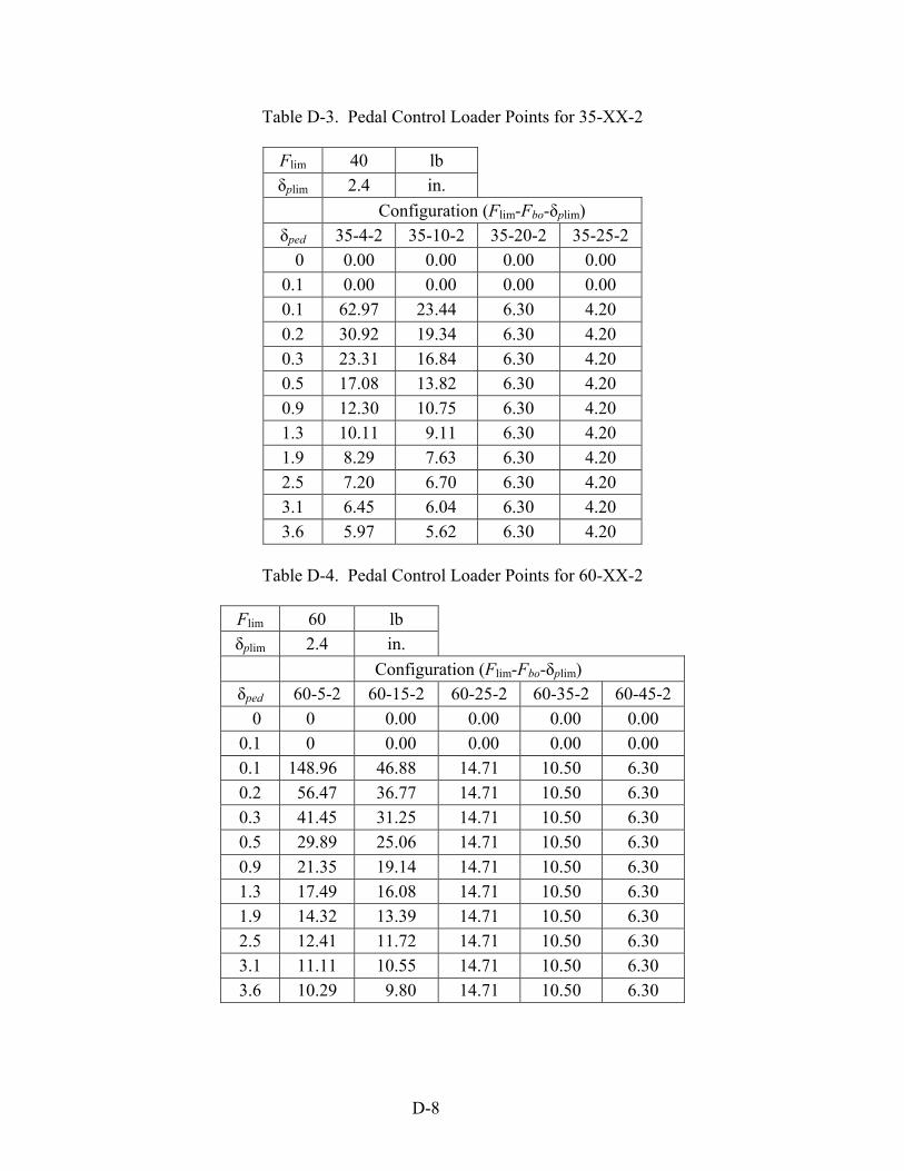
Table D-3. Pedal Control Loader Points for 35-XX-2

Flim 40 lb δplim 2.4 in.

Configuration (Flim-Fbo-δplim) δped 35-4-2 35-10-2 35-20-2 35-25-2 0.0 0.00 00.00 0.00 0.00 0.1 0.00 00.00 0.00 0.00 0.1 62.97 23.44 6.30 4.20 0.2 30.92 19.34 6.30 4.20 0.3 23.31 16.84 6.30 4.20 0.5 17.08 13.82 6.30 4.20 0.9 12.30 10.75 6.30 4.20 1.3 10.11 09.11 6.30 4.20 1.9 8.29 07.63 6.30 4.20 2.5 7.20 06.70 6.30 4.20 3.1 6.45 06.04 6.30 4.20 3.6 5.97 05.62 6.30 4.20

Table D-4. Pedal Control Loader Points for 60-XX-2

Flim 60 lb δplim 2.4 in.

Configuration (Flim-Fbo-δplim) δped 60-5-2 60-15-2 60-25-2 60-35-2 60-45-2 0.0 000 00.00 00.00 00.00 0.00 0.1 000 00.00 00.00 00.00 0.00 0.1 148.96 46.88 14.71 10.50 6.30 0.2 056.47 36.77 14.71 10.50 6.30 0.3 041.45 31.25 14.71 10.50 6.30 0.5 029.89 25.06 14.71 10.50 6.30 0.9 021.35 19.14 14.71 10.50 6.30 1.3 017.49 16.08 14.71 10.50 6.30 1.9 014.32 13.39 14.71 10.50 6.30 2.5 012.41 11.72 14.71 10.50 6.30 3.1 11.11 10.55 14.71 10.50 6.30 3.6 10.29 09.80 14.71 10.50 6.30

D-8

Table D-5. Pedal Control Loader Points for 35-XX-3

Flim 35 lb δplim 3.5 in.

Configuration (Flim-Fbo-δplim) δped 35-4-3 35-10-3 35-20-3 30-25-3 0.0 00.00 00.00 0.00 0.00 0.1 00.00 00.00 0.00 0.00 0.1 43.17 16.07 4.31 2.87 0.2 24.29 13.98 4.31 2.87 0.3 18.72 12.54 4.31 2.87 0.5 13.91 10.63 4.31 2.87 0.9 10.10 08.50 4.31 2.87 1.3 08.32 07.29 4.31 2.87 1.9 06.84 06.17 4.31 2.87 2.5 05.94 05.44 4.31 2.87 3.1 05.32 04.93 4.31 2.87 3.6 04.93 04.59 4.31 2.87

Table D-6. Pedal Control Loader Points for 60-XX-3

Flim 60 lb δplim 3.5 in.

Configuration (Flim-Fbo-δplim) δped 60-5-3 60-15-3 60-25-3 60-35-3 60-45-3 0.0 000.00 00.00 00.00 0.00 0.00 0.1 000.00 00.00 00.00 0.00 0.00 0.1 102.13 32.14 10.06 7.18 4.31 0.2 045.29 26.89 10.06 7.18 4.31 0.3 033.73 23.58 10.06 7.18 4.31 0.5 024.53 19.51 10.06 7.18 4.31 0.9 017.60 15.27 10.06 7.18 4.31 1.3 014.44 12.97 10.06 7.18 4.31 1.9 011.83 10.89 10.06 7.18 4.31 2.5 010.26 09.57 10.06 7.18 4.31 3.1 009.19 08.63 10.06 7.18 4.31 3.6 008.51 08.04 10.06 7.18 4.31

D-9

D.2 CONTROL LOADER PLOTS. To verify that the pedal control loaders were operating as intended, time histories were recorded while a VMS technician, seated in the cab, moved the pedals through the full range of motion (±δplim). Each run was started at full deflection. The resulting time histories (figures D-9 through D-35) show the measured force on the pedal (RUNDUM channel “FORCEPED”) versus pedal displacement, as measured from the motion cab (RUNDUM channel “DPXCAB”). A slight error in force at maximum pedal displacement was found, which was attributed the pedal dead band being changed without recalculation of the gradient points. However, this error was consistent throughout all trials and placed no limitations on data analysis.

-2 -1.5 -1 -0.5 0 0.5 1 1.5 2-40

-30

-20

-10

0

Fpe

d (

lb)

10

20

30

40 Loader Plot, Cfg: 35-4-1

δP

Figure D-9. Pedal Control Loader Fped vs δP (35-4-1)

D-10

-2 -1.5 -1 -0.5 0 0.5 1 1.5 2 -40

-30

-20

-10

0

10

20

30

40

Fpe

d (

lb)

Loader Plot, Cfg: 35-10-1

δP

Figure D-10. Pedal Control Loader Fped vs δP (35-10-1)

-2 -1.5 -1 -0.5 0 0.5 1 1.5 2 -40

-30

-20

-10

0

10

20

30

40 Loader Plot, Cfg: 35-20-1

Fpe

d (

lb)

δP

Figure D-11. Pedal Control Loader Fped vs δP (35-20-1)

D-11

Loader Plot, Cfg: 35-25-1

-2 -40-1.5 -1

40

30

20

10

Fpe

d (

lb)

0

-10

-20

-30

-0.5 0 0.5 1 1.5 2

δP

Figure D-12. Pedal Control Loader Fped vs δP (35-25-1)

-2 -1.5 -1 -0.5 0 0.5 1 1.5 2-80

-60

-40

-20

0

20

40

60

80

Fpe

d (

lb)

Loader Plot, Cfg: 60-5-1

δP

Figure D-13. Pedal Control Loader Fped vs δP (60-5-1)

D-12

-2 -1.5 -1 -0.5 0 0.5 1 1.5 2 -80

-60

-40

-20

0

20

40

60

80 Loader Plot, Cfg: 60-15-1

Fpe

d (

lb)

δP

Figure D-14. Pedal Control Loader Fped vs δP (60-15-1)

Loader Plot, Cfg: 60-25-1

80

2 -1.5 -1

60

40

20

Fpe

d (

lb)

0

-20

-40

-60

--80

-0.5 0 0.5 1 1.5 2

δP

Figure D-15. Pedal Control Loader Fped vs δP (60-25-1)

D-13

-2 -1.5 -1 -0.5 0 0.5 1 1.5 2-80

-60

-40

-20

0

20

40

60

80Loader Plot, Cfg: 60-35-1

Fpe

d (

lb)

δP

Figure D-16. Pedal Control Loader Fped vs δP (60-35-1)

Loader Plot, Cfg: 60-45-1

-2-80 -1.5 -1 -0.5 0 0.5 1 1.5

80

60

40

20

Fpe

d (

lb)

0

-20

-40

-60

2

δP

Figure D-17. Pedal Control Loader Fped vs δP (60-45-1)

D-14

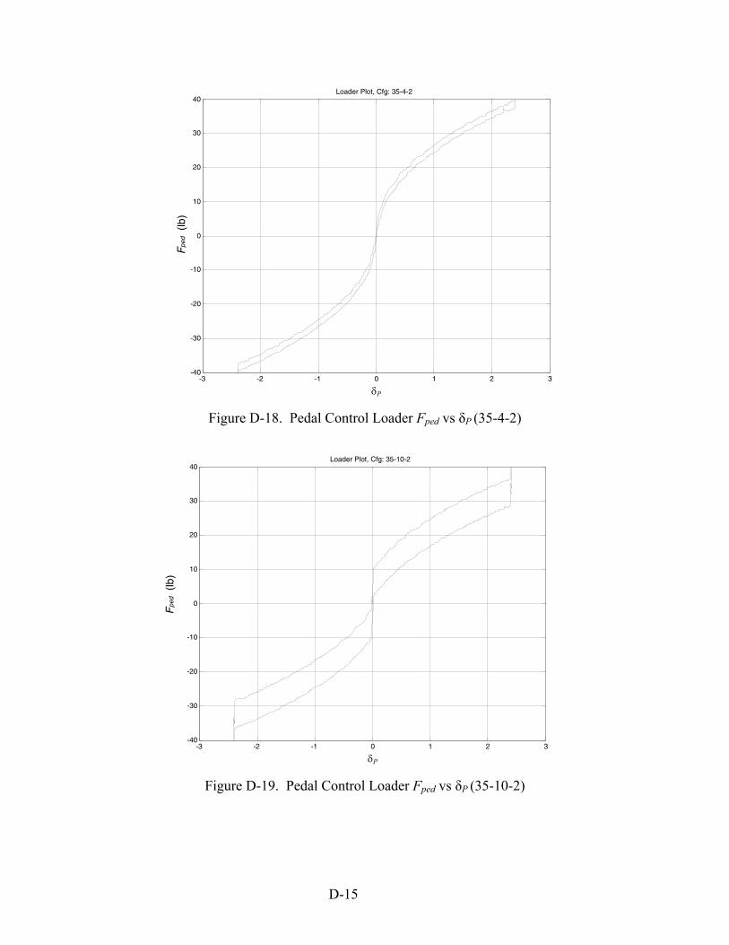
Loader Plot, Cfg: 35-4-2

-3 -40-2

40

30

20

10

Fpe

d (

lb)

0

-10

-20

-30

-1 0 1 2 3

δP

Figure D-18. Pedal Control Loader Fped vs δP (35-4-2)

Loader Plot, Cfg: 35-10-2

-3-40

40

30

20

10

Fpe

d (

lb)

0

-10

-20

-30

-2 -1 0 1 2 3

δP

Figure D-19. Pedal Control Loader Fped vs δP (35-10-2)

D-15

Loader Plot, Cfg: 35-20-2

-3-40

40

30

20

10

Fpe

d (

lb)

0

-10

-20

-30

-2 -1 0 1 2 3

δP

Figure D-20. Pedal Control Loader Fped vs δP (35-20-2)

Loader Plot, Cfg: 35-25-2

-3-40

40

30

20

10

Fpe

d (

lb)

0

-10

-20

-30

-2 -1 0 1 2 3

δP

Figure D-21. Pedal Control Loader Fped vs δP (35-25-2)

D-16

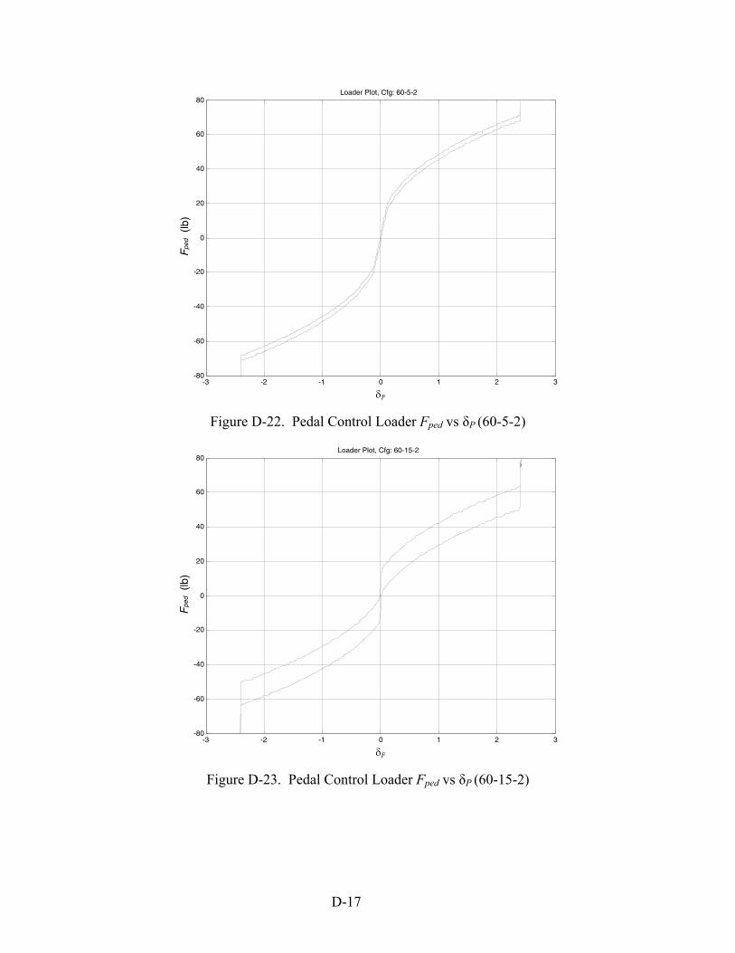
Loader Plot, Cfg: 60-5-2

-3-80

80

60

40

20

Fpe

d (

lb)

0

-20

-40

-60

-2 -1 0 1 2 3

δP

Figure D-22. Pedal Control Loader Fped vs δP (60-5-2)

Loader Plot, Cfg: 60-15-2

-3-80

-2 -1 0

80

60

40

20

Fpe

d (

lb)

0

-20

-40

-60

1 2 3

δP

Figure D-23. Pedal Control Loader Fped vs δP (60-15-2)

D-17

Loader Plot, Cfg: 60-25-280

Figure D-24. Pedal Control Loader Fped vs δP (60-25-2)

Figure D-25. Pedal Control Loader Fped vs δP (60-35-2)

-3 -2 -1 0 1 2 3-80

-60

-40

-20

0

20

40

60

Fpe

d (

lb)

δP

Loader Plot, Cfg: 60-35-280

-3 -2 -1 0 1 2 3-80

-60

-40

-20

0

20

40

60

Fpe

d (

lb)

δP

D-18

Loader Plot, Cfg: 60-45-280

Figure D-26. Pedal Control Loader Fped vs δP (60-45-2)

Figure D-27. Pedal Control Loader Fped vs δP (35-4-3)

-3 -2 -1 0 1 2 3-80

-60

-40

-20

0

20

40

60

Fpe

d (

lb)

δP

Loader Plot, Cfg: 35-4-340

-4 -3 -2 -1 0 1 2 3 4-40

-30

-20

-10

0

10

20

30

Fpe

d (

lb)

δP

D-19

Loader Plot, Cfg: 35-10-340

Figure D-28. Pedal Control Loader Fped vs δP (35-10-3)

Figure D-29. Pedal Control Loader Fped vs δP (35-20-3)

-4 -3 -2 -1 0 1 2 3 4-40

-30

-20

-10

0

10

20

30

Fpe

d (

lb)

δP

Loader Plot, Cfg: 35-20-340

-4 -3 -2 -1 0 1 2 3 4-40

-30

-20

-10

0

10

20

30

Fpe

d (

lb)

δP

D-20

Loader Plot, Cfg: 35-25-340

Figure D-30. Pedal Control Loader Fped vs δP (35-25-3)

Figure D-31. Pedal Control Loader Fped vs δP (60-5-3)

-4 -3 -2 -1 0 1 2 3 4-40

-30

-20

-10

0

10

20

30

Fpe

d (

lb)

δP

Loader Plot, Cfg: 60-5-380

-4 -3 -2 -1 0 1 2 3 4-80

-60

-40

-20

0

20

40

60

Fpe

d (

lb)

δP

D-21

Loader Plot, Cfg: 60-15-380

D-22

Figure D-32. Pedal Control Loader Fped vs δP (60-15-3)

Figure D-33. Pedal Control Loader Fped vs δP (60-25-3)

-4 -3 -2 -1 0 1 2 3 4-80

-60

-40

-20

0

20

40

60

Fpe

d (

lb)

δP

Loader Plot, Cfg: 60-25-380

-4 -3 -2 -1 0 1 2 3 4-80

-60

-40

-20

0

20

40

60

Fpe

d (

lb)

δP

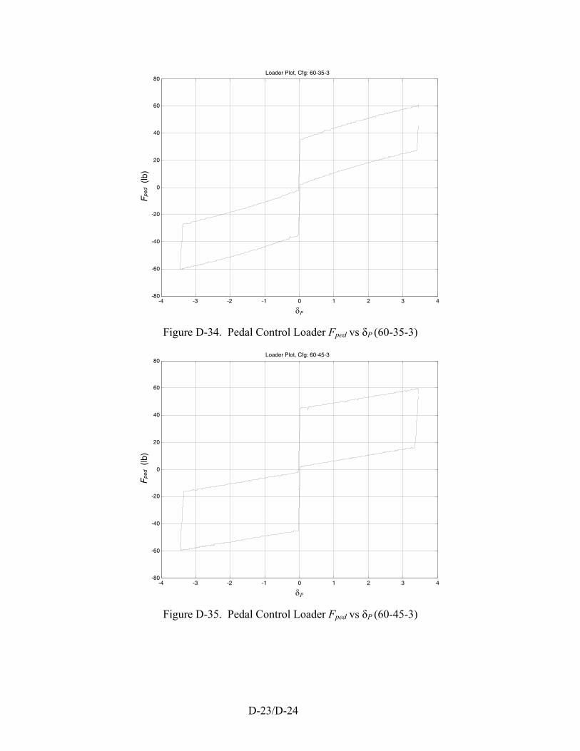
Loader Plot, Cfg: 60-35-380

Figure D-34. Pedal Control Loader Fped vs δP (60-35-3)

Figure D-35. Pedal Control Loader Fped vs δP (60-45-3)

-4 -3 -2 -1 0 1 2 3 4-80

-60

-40

-20

0

20

40

60

Fpe

d (

lb)

δP

Loader Plot, Cfg: 60-45-380

-4 -3 -2 -1 0 1 2 3 4-80

-60

-40

-20

0

20

40

60

Fpe

d (

lb)

δP

D-23/D-24

APPENDIX E—STATISTICS OF VERTICAL STABILIZER FORCE AND r peakβ − δ

Statistical analysis of the simulation data was performed to determine if the peak vertical stabilizer force and r peak

β − δ data are well represented by a normal distribution. This was done

to justify using three standard deviations as representative of the maximum expected value. All first runs were collected for the baseline configurations. Histograms were calculated using the Microsoft® Excel® data analysis tool pack. The bin range in figure E-1 was selected to cover the minimum through maximum vertical stabilizer force in 2000-lb increments. As shown in the histogram, the data is well approximated by a normal distribution with the peak in the vicinity of the mean global average value.

180

Figure E-1. Histogram of Peak Vertical Stabilizer Force

The same analysis was accomplished on the peak values of rβ − δ , with the result shown in figure E-2.

0

30

60

90

120

150

6000 12000 18000 24000 30000 36000

Freq

uenc

y

Peak Vertical Stabilizer Force (lb)

Std Dev |Fv| Peak = 3975 lb (N = 1014)

E-1

0

100

4

E-2

200

300

00

4 6 8 10 12 14

y

Std Dev |β‐δr|Peak = 1.18 deg (N =  1014)

Freq

uenc

y

(lb) r peakβ − δ

Figure E-2. Histogram of r peakβ − δ

APPENDIX F—LINEARITY INDEX

F.1 CALCULATION AND APPLICATION OF THE LINEARITY INDEX TO FORCE-FEEL CURVES. As discussed in references F-1 and F-2, the linearity index (LI) is a measure of how linear a force-feel system appears to the human operator. The metric is calculated as follows.

( ) (1( )

AREA DAHD AREA JHIJLIAREA DEBFD

)+= − (F-1)

The bold lines (ABCDA) on the force-feel curve shown in figure F-1 represent the amount of pedal displacement that is used to deflect the control surface. The remaining part of the curve (BHICB) represents a portion of the force-feel curve in which pedal displacement does not result in rudder displacement. Analogous to a situation where the rudder limit has been reached, while the control is allowed, either by mechanical means or by deformation of control linkage or cable stretch, to displace further (the scale has been exaggerated for clarity). As shown in equation F-1, the LI requires that three separate areas are obtained from the force-feel curve. Figure F-1 shows the AREA(DAHDA) is outlined by connecting the origin (D) to the breakout force (A), following the upstroke of the force-feel curve from point A to point H, and directly back to the origin at point D. The AREA(JHIJ) is outlined by points H, I, and where the line intersects the down stroke of the force-feel curve at point J1. The last area, AREA(DEBFD), is simply the rectangle formed by the points corresponding to the control force at maximum surface deflection, and the corresponding control deflection. For clarity, these areas are identified, shaded, and labeled in figure F-2, and equation F-1 becomes LI = [Area (1) + Area(2)]/Area(3).

BH

ICJ

A (Fbo)

D Fδp

δp lim

E

Fped

Fhb

Figure F-1. Generic Nonlinear Load-Feel Curve Typical of Transport Aircraft

1If the curve representing the downstroke of the pedal does not intersect line DH, then J is at the origin (coincident with D).

F-1

2 3

1

Figure F-2. Identification of Linear Index Area Components

This metric, as shown in figures F-1 and F-2, delineates the differences in force-feel system design with pilots performing a closed-loop tracking task with some caveats. LI is not an absolute scale. This metric is used to make comparisons of two or more different force-feel systems, and as noted, an LI value of 1.0 does not necessarily suggest that the force-feel system is ideal. For instance, if the control throw is too short or the control force at maximum displacement is too high, these factors could contribute to a poor pilot opinion of the force-feel system from a handling qualities perspective regardless of the LI value. A suggested lower limit of 0.6 is proposed as a criterion boundary in reference F-1. F.2 SIMULATED LOAD-FEEL CURVES AND AREA SEGMENT CALCULATION OF ANALYTICAL LOAD-FEEL CURVES. Application of LI to the analytical pedal displacement curves is rather straight forward, as each area of the curve is defined in terms of known quantities. AREA(DAHD), shaded area 1 on figure F-2, is calculated as follows:

lim lim lim1 0

limlim

p bop bo p

pp

F F FA Fδ⎡ ⎤−⎢= δ + −

δδ⎢ ⎥⎣ ⎦∫ pd⎥δ δ (F-2)

AREA(DIHD), shaded area 2 on figure F-2, is calculated as follows:

lim limlim2

lim lim

2p cf hb

p pXp p

F F FFA δ⎡ ⎤− −⎢= δ − δ +δ δ⎢ ⎥⎣ ⎦

∫ hb pF d⎥ δ (F-3)

F-2

Where X is the intersection of the down stroke curve and DH (point J in figure F-2), calculated from the following quadratic:

22 lim 2lim lim

lim limlim

20 2cf hb

hb hbp pp

F F FF FX F X⎡ ⎤⎛ ⎞− −⎢⎜ ⎟= − + +⎢⎜ ⎟δ δδ⎝ ⎠⎣ ⎦

F⎥⎥

m

(F-4)

Pedal force-feel curves of the current study were of the type that points B and H were coincident, meaning that, statically, the rudder was displaced linearly throughout the entire range of pedal motion. Therefore, calculation of AREA(DEBFD) , area 3 on figure F-2, was simply: 3 lim lipA F= δ (F-5) Calculation of area 1 for the linear force-feel systems was as follows:

lim lim lim1 0

lim lim

( ) p bop bo p

p p

F F FA Fδ ⎡ ⎤−= δ + −⎢

δ δ⎢ ⎥⎣ ⎦∫ pdδ δ⎥ (F-6)

Calculation of area 2 for the linear force-feel systems was as follows:

lim limlim2

lim lim

2( ) p cf hb

p pXp p

F F FFA δ ⎡ ⎤− −= δ − δ +⎢

δ δ⎢ ⎥⎣ ⎦∫ hb pF dδ⎥ (F-7)

Where X for the linear force-feel systems being calculated as:

limlim

lim lim

2hb

cf hb

p p

FXF F FF

=⎛ ⎞− −

−⎜ ⎟⎜ ⎟δ δ⎝ ⎠

(F-8)

To account for errors between the analytical and actual force-feel curves, the analytical values for Flim were modified with the changes found in table F-1.

F-3

Table F-1. Corrected Parameters and Reconciliation of Analytical and Actual Force-Feel Curves

Analytical 35 Analytical 60 Recorded 39 Recorded 68

35-4-1

Error 4

60-5-1

Error 8 Analytical 35 Analytical 60 Recorded 37 Recorded 64

35-10-1

Error 2

60-15-1

Error 4 Analytical 35 Analytical 60 Recorded 35 Recorded 61

35-20-1

Error 0

60-25-1

Error 1 Analytical 35 Analytical 60 Recorded 35 Recorded 60

35-25-1

Error 0

60-35-1

Error 0 Analytical 60 Recorded 60

60-45-1

Error 0 Analytical 35 Analytical 60 Recorded 39.5 Recorded 71

35-4-2

Error 4.5

60-5-2

Error 11 Analytical 35 Analytical 60 Recorded 36 Recorded 63

35-10-2

Error 1

60-15-2

Error 3 Analytical 35 Analytical 60 Recorded 35 Recorded 61

35-20-2

Error 0

60-25-2

Error 1 Analytical 35 Analytical 60 Recorded 35 Recorded 60

35-25-2

Error 0

60-35-2

Error 0 Analytical 60 Recorded 60

60-45-2

Error 0 Analytical 35 Analytical 60 Recorded 39 Recorded 69

35-4-3

Error 4

60-5-3

Error 9 Analytical 36.5 Analytical 60 Recorded 36.5 Recorded 63

35-10-3

Error 0

60-15-3

Error 3 Analytical 35 Analytical 60 Recorded 35 Recorded 61

35-20-3

Error 0

60-25-3

Error 1 Analytical 35 Analytical 60 Recorded 35 Recorded 60

35-25-3

Error 0

60-35-3

Error 0 Analytical 60 Recorded 60

60-45-3

Error 0

F-4

Having made the necessary adjustments to the analytical force-feel curves, the associated areas and LIs were calculated. The results are shown in table F-2. Example overlays of the analytical and actual pedal force-feel curve are shown in figure F-3.

Table F-2. Calculated Linear Index Parameters for the Force-Feel Curves

Force Curve No.

Flim (lb)

Fbo (lb)

δplim (in.)

Fcf (lb)

Fhb (lb) A** B** C**

X (in.)

A1 (in-lb)

A2 (in-lb)

A3 (in-lb) LI

35-4-1 39 4 1.2 1 2 1056.3 -1168.1 24.8 1.08 8.9 0.1 46.8 0.81 35-10-1 37 10 1.2 4 2 950.7 -741.1 16.4 0.76 10.8 1.7 44.4 0.72 35-20-1 35 20 1.2 9 2 NA NA NA 0.12 11.5 9.8 42.0 0.49 35-25-1 35 25 1.2 11.5 2 NA NA NA 0.10 14.4 12.8 42.0 0.35 35-4-2 39.5 4 2.4 1 2 270.9 -595.4 14.6 2.17 18.4 0.2 94.8 0.80 35-10-2 36 10 2.4 4 2 225.0 -344.0 9.7 1.50 21.9 3.5 86.4 0.71 35-20-2 35 20 2.4 9 2 NA NA NA 0.24 23.5 19.6 84.0 0.49 35-25-2 35 25 2.4 11.5 2 NA NA NA 0.19 29.4 25.5 84.0 0.35 35-4-3 39 4 3.5 1 2 124.2 -396.6 11.0 3.17 26.9 0.3 136.5 0.80 35-10-3 36.5 10 3.5 4 2 108.8 -243.5 8.0 2.21 32.4 5.0 127.8 0.71 35-20-3 35 20 3.5 9 2 NA NA NA 0.35 34.5 28.5 122.5 0.49 35-25-3 35 25 3.5 11.5 2 NA NA NA 0.28 43.2 37.1 122.5 0.34 60-5-1 68 5 1.2 1.5 2 3211.1 -3590.2 71.3 1.10 14.7 0.2 81.6 0.82 60-15-1 64 15 1.2 6.5 2 2844.4 -2248.1 44.7 0.77 17.9 2.7 76.8 0.73 60-25-1 61 25 1.2 11.5 2 NA NA NA 0.10 14.2 13.0 73.2 0.63 60-35-1 60 35 1.2 16.5 2 NA NA NA 0.07 20.1 18.9 72.0 0.46 60-45-1 60 45 1.2 21.5 2 NA NA NA 0.05 26.0 24.8 72.0 0.30 60-5-2 71 5 2.4 1.5 2 875.2 -1948.6 40.6 2.21 31.4 0.3 170.4 0.81 60-15-2 63 15 2.4 6.5 2 689.1 -1073.1 23.4 1.54 36.3 5.5 151.2 0.72 60-25-2 61 25 2.4 11.5 2 NA NA NA 0.19 29.1 25.7 146.4 0.63 60-35-2 60 35 2.4 16.5 2 NA NA NA 0.14 41.1 37.6 144.0 0.45 60-45-2 60 45 2.4 21.5 2 NA NA NA 0.11 53.0 49.4 144.0 0.29 60-5-3 69 5 3.5 1.5 2 388.7 -1255.9 27.5 3.21 45.1 0.4 241.5 0.81 60-15-3 63 15 3.5 6.5 2 324.0 -734.1 17.2 2.24 53.3 8.0 220.5 0.72 60-25-3 61 25 3.5 11.5 2 NA NA NA 0.28 42.9 37.3 213.5 0.62 60-35-3 60 35 3.5 16.5 2 NA NA NA 0.20 60.3 54.7 210.0 0.45 60-45-3 60 45 3.5 21.5 2 NA NA NA 0.16 77.7 72.0 210.0 0.29 **A, B, and C used for quadratic equation are not applicable (NA) for linear force-feel curves.

F-5

0

10

20

30

40

50

60

70

0 0.5 1 1.5 2 2.5 3 3.5

FPED(lb)

δ p (in)

Analytical

Actual

Figure F-3. Overlay of Analytical and Actual Force-Feel Curves Used in the Study

F.3 RELATIONSHIP OF LINEAR INDEX TO Fbo/Flim. Another parameter explored in this study was the ratio of the breakout force to the limit force Fbo/Flim. As it turns out, this ratio is closely related to LI. Consider the force-feel curve (60-45-3) shown in figure F-4.

0

10

20

30

40

50

60

0 0.5 1 1.5 2 2.5 3 3

FPED(lb)

.5δ p (in)

Fbo 2Fcf

δplim Fhb

Figure F-4. Analytical and Actual Force-Feel Curves of Configuration 60-45-3

F-6

The calculation of areas 1 and 2 can be approximated by the areas of a triangle:

112 bo pA F lim= δ (F-9)

( )2 li1 2 (2 cf p m )A F= δ − X

lim

(F-10)

Area 3 for this configuration is calculated as: 3 cf pA F= δ (F-11) Calculation of LI then becomes:

( )lim lim

lim lim

1 1 2 (2 21

bo p cf p

p

F FLI

F

δ + δ −= −

δ

)X (F-12)

For all current study configurations, the following was true: 2bo cf hbF F F= + (F-13) With the approximation of LI becoming:

lim lim

lim lim

1 1 ( )(2 21

bo p bo hb p

p

F F FLI

F

δ + − δ −= −

δ

)X (F-14)

Which then reduces to:

lim lim lim lim lim

12 2

bo hb bo hb

p

F F F FXLIF F F F

⎛= − + + −⎜δ ⎝ ⎠

⎞⎟ (F-15)

For the tested configurations in this study, the ratio lim

boFF

was the dominant term, resulting in an

approximation of LI as:

lim

1 boFLIF

=∼ (F-16)

As shown in figure F-5, the calculated and approximated values of LI are in close agreement for all the tested configurations.

F-7

0

0.2

0.4

0.6

0.8

1

1.2

0.00 0.20 0.40 0.60 0.80

LI and1‐Fbo/Flim

Fbo/Flim

LI 1‐FBO/FLIM

Figure F-5. Comparison of LI and Approximation From Fbo/Flim

Both Fbo/Flim and LI were considered as candidate metrics for an overcontrol criterion. As shown by equation F-16 and figure F-5, these parameters turn out to be very closely correlated. Nonetheless, both were tested against the simulation data with the results shown in section 5.3 of the main report. As expected, both parameters showed, essentially, identical trends. Neither parameter was sensitive to overcontrol tendency or to the maximum force imposed on the vertical stabilizer; therefore, and they were rejected as potential criterion parameters. This analysis shows that for load-feel curves that have the characteristics of those used in this simulation (which is representative of essentially all transport aircraft), Fbo/Flim and LI may be used interchangeably. F.4 REFERENCES. F-1. Hess, R.A., “Rudder Control Strategies and Force/Feel System Designs in Transport

Aircraft,” Journal of Guidance, Control, and Dynamics, Vol. 28, Number 6, pp. 1251-1262, December 2005.

F-2. Hess, R.A., “Preliminary Assessment of Design Metrics for Transport Aircraft Rudder

Control Systems,” A Presentation at NASA Langley.

F-8

APPENDIX G—MATLAB SIMULINK MODEL

To investigate how changes in yaw damper performance could affect experimental metrics the lateral/directional equations of motion for a transport aircraft were modeled in Simulink®. The Convair CV-880M transport aircraft model was used (figure G-1). Derivatives and mass properties were obtained from reference G-1. The chosen flight condition was cruise at 23,000 ft, M = 0.6 (615 ft/s). The state-space equations of motion Code Listing is shown on page G-2.

Figure G-1. Convair CV-880M Transport

G-1

G-2

Code Listing % Convair 880M Lateral Directional Derivatives % From Hefley, pp 205 g = 32.2; VT0 = 615; U0 = VT0*cos(5.3/57.3); W0 = U0*sin(5.3/57.3); alpha0 = (5.3)/57.3; Yv = -0.115; Yp = 0; Yr = 0; Lbeta_p = -5.98; Lp_p = -1.14; Lr_p = 0.434; Nbeta_p = 1.42; Np_p = -0.0416; Nr_p = -0.188; YdeltaR = 0.0245; YdeltaA = -0.00458; LdeltaR = 0.806; LdeltaA = 2.85; NdeltaR = -0.926; NdeltaA = 0.23; lz = 0; lx = 0; KTC = 0.1/57.3; KAY = (0.09)/57.3; KBD = (1.30);%/57.3; gct = g*cos(alpha0); dplim = 1.2; drlim = 9/57.3; KPED = drlim/dplim; A = [ Yv (W0-Yp)/VT0 (-U0+Yr)/VT0*cos(alpha0) g*cos(alpha0)/VT0 ; Lbeta_p Lp_p Lr_p 0 ; Nbeta_p Np_p Nr_p 0 ; 0 1 tan(alpha0) 0 ]; B = [ YdeltaA YdeltaR 0; LdeltaA LdeltaR Lp_p; NdeltaA NdeltaR 0; 0 0 0]; C = [ 1 0 0 0; 0 1 0 0; 0 0 1 0; 0 0 0 1; Yv (W0-Yp)/VT0 (-U0+Yr)/VT0*cos(alpha0) g*cos(alpha0)/VT0 ; Lbeta_p Lp_p Lr_p 0 ; Nbeta_p Np_p Nr_p 0 ]; D = [ 0 0 0; 0 0 0; 0 0 0; 0 0 0; YdeltaA YdeltaR 0; LdeltaA LdeltaR 0; NdeltaA NdeltaR 0]; states = { 'beta'; 'p'; 'r'; 'phi'}; inputs = { 'a'; 'r' 'pg'}; CON880M = ss(A,B,C,D,'StateName',states,'InputName',inputs); [num1 den1] = ss2tf(A,B,C,D,1); [num2 den1] = ss2tf(A,B,C,D,2); betada = tf(num1(1,:),den1); pda = tf(num1(2,:),den1); rda = tf(num1(3,:),den1); phida = tf(num1(4,:),den1); frees = tf([1 0],1); ayda = VT0*frees*betada-W0*pda+U0*rda-g*cos(alpha0)*phida;

The lateral directional CV-880M model (figure G-2) was augmented with an identical yaw damper, as used in the simulation trials.

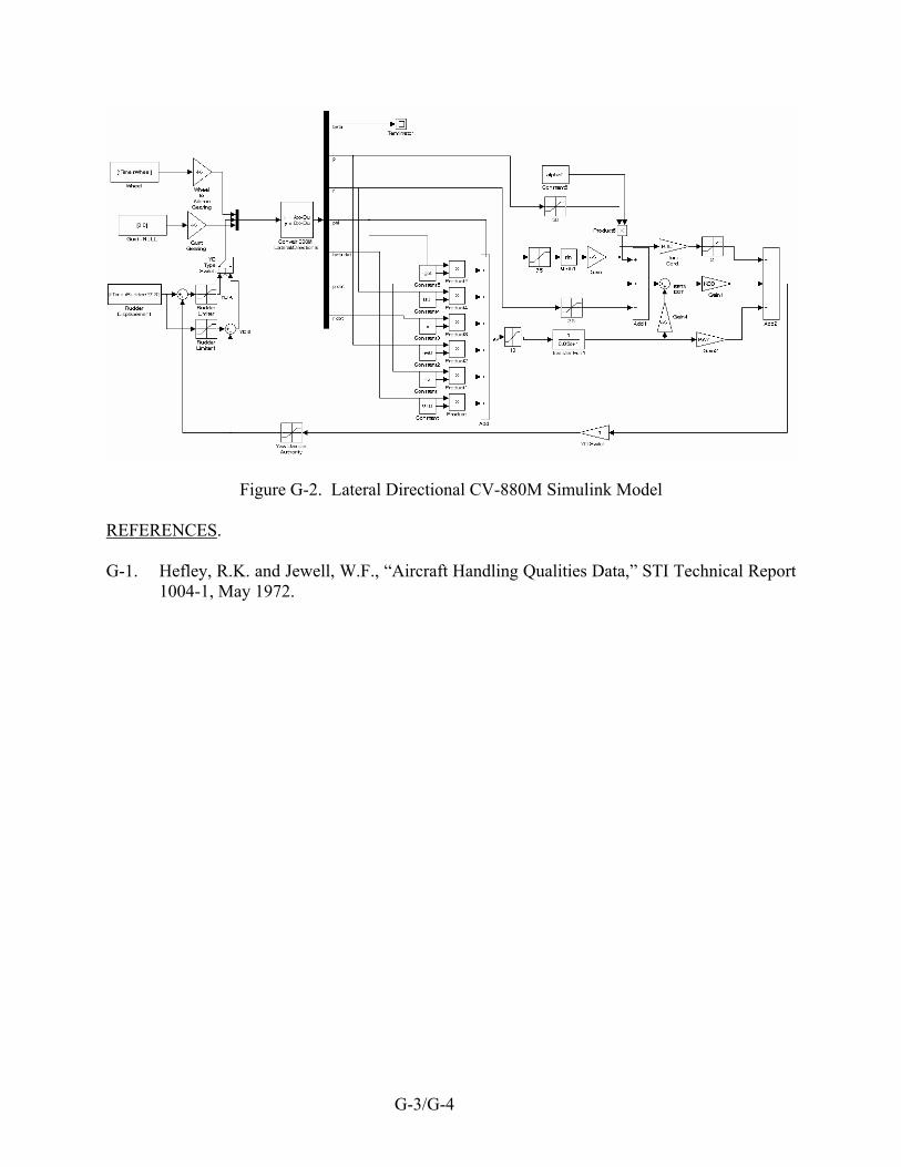
Figure G-2. Lateral Directional CV-880M Simulink Model REFERENCES.

G-1. Hefley, R.K. and Jewell, W.F., “Aircraft Handling Qualities Data,” STI Technical Report

1004-1, May 1972.

G-3/G-4