Dostoevsky: Better Space-Time Trade-Offs for LSM-Tree BasedKey-Value Stores via Adaptive Removal of Superfluous Merging

Niv Dayan, Stratos IdreosHarvard University

ABSTRACTWe show that all mainstream LSM-tree based key-value stores in theliterature and in industry suboptimally trade between the I/O cost ofupdates on one hand and the I/O cost of lookups and storage spaceon the other. The reason is that they perform equally expensivemerge operations across all levels of LSM-tree to bound the numberof runs that a lookup has to probe and to remove obsolete entriesto reclaim storage space. With state-of-the-art designs, however,merge operations from all levels of LSM-tree but the largest (i.e.,most merge operations) reduce point lookup cost, long range lookupcost, and storage space by a negligible amount while significantlyadding to the amortized cost of updates.

To address this problem, we introduce Lazy Leveling, a new de-sign that removes merge operations from all levels of LSM-tree butthe largest. Lazy Leveling improves the worst-case complexity ofupdate cost while maintaining the same bounds on point lookupcost, long range lookup cost, and storage space. We further intro-duce Fluid LSM-tree, a generalization of the entire LSM-tree designspace that can be parameterized to assume any existing design.Relative to Lazy Leveling, Fluid LSM-tree can optimize more forupdates by merging less at the largest level, or it can optimize morefor short range lookups by merging more at all other levels.

We put everything together to design Dostoevsky, a key-valuestore that adaptively removes superfluous merging by navigatingthe Fluid LSM-tree design space based on the application workloadand hardware. We implemented Dostoevsky on top of RocksDB,and we show that it strictly dominates state-of-the-art designs interms of performance and storage space.

ACM Reference Format:Niv Dayan, Stratos Idreos. 2018. Dostoevsky: Better Space-Time Trade-Offsfor LSM-Tree Based Key-Value Stores via Adaptive Removal of SuperfluousMerging . In Proceedings of 2018 International Conference on Management ofData (SIGMOD’18). ACM, New York, NY, USA, 16 pages. https://doi.org/10.1145/3183713.3196927

1 INTRODUCTIONKey-Value Stores and LSM-Trees. A key-value store is a data-base that efficiently maps from search keys to their correspond-ing data values. Key-value stores are used everywhere today fromgraph processing in social media [8, 17] to event log processing in

Permission to make digital or hard copies of all or part of this work for personal orclassroom use is granted without fee provided that copies are not made or distributedfor profit or commercial advantage and that copies bear this notice and the full citationon the first page. Copyrights for components of this work owned by others than ACMmust be honored. Abstracting with credit is permitted. To copy otherwise, or republish,to post on servers or to redistribute to lists, requires prior specific permission and/or afee. Request permissions from permissions@acm.org.SIGMOD’18, June 10–15, 2018, Houston, TX, USA© 2018 Association for Computing Machinery.ACM ISBN 978-1-4503-4703-7/18/06. . . $15.00https://doi.org/10.1145/3183713.3196927

WiredTiger

RocksDB, LevelDB, cLSM

bLSM

Cassandra, HBase

Dostoevsky

faster lookups

fasterupdates Monkey

update cost

poin

t lo

okup &

space c

ost

s

log

sortedarray

Monkey optimizes the Bloom filters allocation

Mainstream designs strike suboptimal trade-offs

Dostoevsky removes superfluous merging

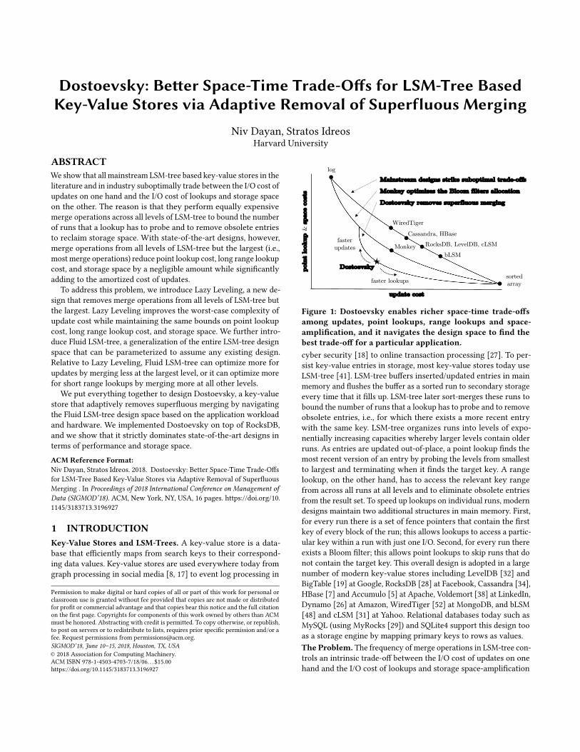
Figure 1: Dostoevsky enables richer space-time trade-offsamong updates, point lookups, range lookups and space-amplification, and it navigates the design space to find thebest trade-off for a particular application.cyber security [18] to online transaction processing [27]. To per-sist key-value entries in storage, most key-value stores today useLSM-tree [41]. LSM-tree buffers inserted/updated entries in mainmemory and flushes the buffer as a sorted run to secondary storageevery time that it fills up. LSM-tree later sort-merges these runs tobound the number of runs that a lookup has to probe and to removeobsolete entries, i.e., for which there exists a more recent entrywith the same key. LSM-tree organizes runs into levels of expo-nentially increasing capacities whereby larger levels contain olderruns. As entries are updated out-of-place, a point lookup finds themost recent version of an entry by probing the levels from smallestto largest and terminating when it finds the target key. A rangelookup, on the other hand, has to access the relevant key rangefrom across all runs at all levels and to eliminate obsolete entriesfrom the result set. To speed up lookups on individual runs, moderndesigns maintain two additional structures in main memory. First,for every run there is a set of fence pointers that contain the firstkey of every block of the run; this allows lookups to access a partic-ular key within a run with just one I/O. Second, for every run thereexists a Bloom filter; this allows point lookups to skip runs that donot contain the target key. This overall design is adopted in a largenumber of modern key-value stores including LevelDB [32] andBigTable [19] at Google, RocksDB [28] at Facebook, Cassandra [34],HBase [7] and Accumulo [5] at Apache, Voldemort [38] at LinkedIn,Dynamo [26] at Amazon, WiredTiger [52] at MongoDB, and bLSM[48] and cLSM [31] at Yahoo. Relational databases today such asMySQL (using MyRocks [29]) and SQLite4 support this design tooas a storage engine by mapping primary keys to rows as values.The Problem. The frequency of merge operations in LSM-tree con-trols an intrinsic trade-off between the I/O cost of updates on onehand and the I/O cost of lookups and storage space-amplification

(i.e., caused by the presence of obsolete entries) on the other. Theproblem is that existing designs trade suboptimally among thesemetrics. Figure 1 conceptually depicts this by plotting point lookupcost and space-amplification on the y-axis against update cost onthe x-axis (while these y-axis metrics have different units, theirtrade-off curves with respect to the x-axis have the same shape).The two points at the edges of the curves are a log and a sortedarray. LSM-tree degenerates into these edge points when it doesnot merge at all or when it merges as much as possible, respectively.We place mainstream systems along the top curve between theseedge points based on their default merge frequencies, and we drawa superior trade-off curve for Monkey [22], which represents thecurrent state of the art. We show that there exists an even supe-rior trade-off curve to Monkey. Existing designs forgo a significantamount of performance and/or storage space for not being designedalong this bottom curve.The Problem’s Source. By analyzing the design space of state-of-the-art LSM-trees, we pinpoint the problem to the fact that theworst-case update cost, point lookup cost, range lookup cost, andspace-amplification derive differently from across different levels.• Updates. The I/O cost of an update is paid later throughthe merge operations that the updated entry participates in.While merge operations at larger levels entail exponentiallymore work, they take place exponentially less frequently.Therefore, updates derive their I/O cost equally from mergeoperations across all levels.• Point lookups. While mainstream designs along the topcurve in Figure 1 set the same false positive rate to Bloomfilters across all levels of LSM-tree, Monkey, the currentstate of the art, sets exponentially lower false positive rates toBloom filters at smaller levels [22]. This is shown tominimizethe sum of false positive rates across all filters and to therebyminimize I/O for point lookups. At the same time, this meansthat access to smaller levels is exponentially less probable.Therefore, most point lookup I/Os target the largest level.• Long range lookups1. As levels in LSM-tree have exponen-tially increasing capacities, the largest level contains mostof the data, and so it tends to contain most of the entrieswithin a given key-range. Therefore, most I/Os issued bylong range lookups target the largest level.• Short range lookups. Range lookups with extremely smallkey ranges only access approximately one block within eachrun regardless of the run’s size. As the maximum number ofruns per level is fixed in state-of-the-art designs, short rangelookups derive their I/O cost equally from across all levels.• Space-Amplification. The worst-case space-amplificationoccurs when all entries at smaller levels are updates to entriesat the largest level. Therefore, the highest fraction of obsoleteentries in the worst-case is at the largest level.

Since the worst-case point lookup cost, long range lookup costand space-amplification derive mostly from the largest level, mergeoperations at all levels of LSM-tree but the largest (i.e., most mergeoperations) hardly improve on these metrics while significantlyadding to the amortized cost of updates. This leads to suboptimaltrade-offs. We solve this problem from the ground up in three steps.1In Section 3, we distinguish formally between short and long range lookups.

Solution 1: Lazy Leveling to Remove Superfluous Merging.We expand the LSM-tree design space with Lazy Leveling, a new de-sign that removes merging from all but the largest level of LSM-tree.Lazy Leveling improves the worst-case cost complexity of updateswhile maintaining the same bounds on point lookup cost, longrange lookup cost, and space-amplification and while providing acompetitive bound on short range lookup cost. We show that theimproved update cost can be traded to reduce point lookup cost andspace-amplification. This generates the bottom curve in Figure 1,which offers richer space-time trade-offs that have been impossibleto achieve with state-of-the-art designs until now.

Solution 2: Fluid LSM-Tree for Design Space Fluidity. We in-troduce Fluid LSM-tree as a generalization of LSM-tree that enablestransitioning fluidly across the whole LSM-tree design space. FluidLSM-tree does this by controlling the frequency of merge opera-tions separately for the largest level and for all other levels. Relativeto Lazy Leveling, Fluid LSM-tree can optimize more for updates bymerging less at the largest level, or it can optimize more for shortrange lookups by merging more at all other levels.

Solution 3: Dostoevsky to Navigate the Design Space.We puteverything together in Dostoevsky: Space-Time Optimized Evol-vable Scalable Key-Value Store. Dostoevsky analytically finds thetuning of Fluid LSM-tree that maximizes throughput for a particularapplication workload and hardware subject to a user constrainton space-amplification. It does this by pruning the search spaceto quickly find the best tuning and physically adapting to it dur-ing runtime. Since Dostoevsky spans all existing designs and isable to navigate to the best one for a given application, it strictlydominates existing key-value stores in terms of performance andspace-amplification. We depict Dostoevsky in Figure 1 as a blackstar that can navigate the entire design space.

Contributions. Our contributions are summarized below.

• We show that state-of-the-art LSM-trees perform equallyexpensive merge operations across all levels of LSM-tree, yetmerge operations at all but the largest level (i.e., most mergeoperations) improve point lookup cost, long range lookupcost, and space-amplification by a negligible amount whileadding significantly to the amortized cost of updates.• We introduce Lazy Leveling to remove merge operations atall but the largest level. This improves the cost complexityof updates while maintaining the same bounds on pointlookups, long range lookups, and space-amplification andwhile providing a competitive bound on short range lookups.• We introduce Fluid LSM-tree, a generalization of LSM-treethat spans all existing designs. Relative to Lazy Leveling,Fluid LSM-tree can optimize more for updates by mergingless at the largest level, or it can optimize more for shortrange lookups by merging more at all other levels.• We introduce Dostoevsky, a key-value store that dynamicallyadapts across the Fluid LSM-tree design space to the designthat maximizes the worst-case throughput based on the ap-plication workload and the hardware subject to a constrainton space-amplification.• We implemented Dostoevsky on RocksDB and show that itdominates existing designs for any application scenario.

4

fence pointers

buffer

Bloom filters

mai

n m

emor

yse

condar

y s

tora

ge

level 1 2

7

3

1

2568

1347

tiering

4

0 1 2

137

leveling

12345678

0

2568

… …

sorted runs

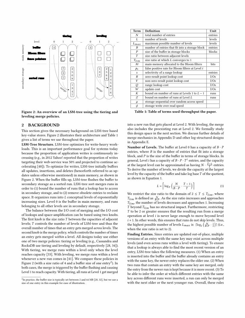
Figure 2: An overview of an LSM-tree using the tiering andleveling merge policies.

2 BACKGROUNDThis section gives the necessary background on LSM-tree basedkey-value stores. Figure 2 illustrates their architecture and Table 1gives a list of terms we use throughout the paper.LSM-Tree Structure. LSM-tree optimizes for write-heavy work-loads. This is an important performance goal for systems todaybecause the proportion of application writes is continuously in-creasing (e.g., in 2012 Yahoo! reported that the proportion of writestargeting their web-service was 50% and projected to continue ac-celerating [48]). To optimize for writes, LSM-tree initially buffersall updates, insertions, and deletes (henceforth referred to as up-dates unless otherwise mentioned) in main memory, as shown inFigure 2. When the buffer fills up, LSM-tree flushes the buffer tosecondary storage as a sorted run. LSM-tree sort-merges runs inorder to (1) bound the number of runs that a lookup has to accessin secondary storage, and to (2) remove obsolete entries to reclaimspace. It organizes runs into L conceptual levels of exponentiallyincreasing sizes. Level 0 is the buffer in main memory, and runsbelonging to all other levels are in secondary storage.

The balance between the I/O cost of merging and the I/O costof lookups and space-amplification can be tuned using two knobs.The first knob is the size ratio T between the capacities of adjacentlevels; T controls the number of levels of LSM-tree and thus theoverall number of times that an entry gets merged across levels. Thesecond knob is themerge policy, which controls the number of timesan entry gets merged within a level. All designs today use eitherone of two merge policies: tiering or leveling (e.g., Cassandra andRocksDB use tiering and leveling by default, respectively [28, 34]).With tiering, we merge runs within a level only when the levelreaches capacity [33]. With leveling, we merge runs within a levelwhenever a new run comes in [41]. We compare these policies inFigure 2 (with a size ratio of 4 and a buffer size of one entry2). Inboth cases, the merge is triggered by the buffer flushing and causingLevel 1 to reach capacity. With tiering, all runs at Level 1 get merged

2In practice, the buffer size is typically set between 2 and 64 MB [28, 32], but we use asize of one entry in this example for ease of illustration.

Term Definition UnitN total number of entries entriesL number of levels levels

Lmax maximum possible number of levels levelsB number of entries that fit into a storage block entriesP size of the buffer in storage blocks blocksT size ratio between adjacent levels

Tl im size ratio at which L converges to 1M main memory allocated to the Bloom filters bitspi false positive rate for Bloom filters at Level is selectivity of a range lookup entriesR zero-result point lookup cost I/OsV non-zero-result point lookup cost I/OsQ range lookup cost I/OsW update cost I/OsK bound on number of runs at Levels 1 to L − 1 runsZ bound on number of runs at Level L runsµ storage sequential over random access speedϕ storage write over read speed

Table 1: Table of terms used throughput the paper.

into a new run that gets placed at Level 2. With leveling, the mergealso includes the preexisting run at Level 2. We formally studythis design space in the next section. We discuss further details ofmerge mechanics in Appendix D and other log-structured designsin Appendix E.Number of Levels. The buffer at Level 0 has a capacity of B · Pentries, where B is the number of entries that fit into a storageblock, and P is the size of the buffer in terms of storage blocks. Ingeneral, Level i has a capacity of B · P ·T i entries, and the capacityat the largest level can be approximated as having N · T−1T entries.To derive the number of levels, we divide the capacity at the largestlevel by the capacity of the buffer and take log baseT of the quotient,as shown in Equation 1.

L =⌈logT

( NB · P

·T − 1T

) ⌉(1)

We restrict the size ratio to the domain of 2 ≤ T ≤ Tl im , whereTl im is defined as N

B ·P . As the size ratio increases and approachesTl im , the number of levels decreases and approaches 1. IncreasingT beyond Tl im has no structural impact. Furthermore, restrictingT to be 2 or greater ensures that the resulting run from a mergeoperation at level i is never large enough to move beyond leveli + 1. In other words, this ensures that runs do not skip levels. Thus,the highest possible number of levels Lmax is ⌈log2

(NB ·P ·

12

)⌉ (i.e.,

when the size ratio is set to 2).Finding Entries. Since entries are updated out-of-place, multipleversions of an entry with the same key may exist across multiplelevels (and even across runs within a level with tiering). To ensurethat a lookup is always able to find the most recent version of anentry, LSM-tree takes the following measures. (1) When an entryis inserted into the buffer and the buffer already contains an entrywith the same key, the newer entry replaces the older one. (2) Whentwo runs that contain an entry with the same key are merged, onlythe entry from the newer run is kept because it is more recent. (3) Tobe able to infer the order at which different entries with the samekey across different runs were inserted, a run can only be mergedwith the next older or the next younger run. Overall, these rules

ensure that if there are two runs that contain different versions ofthe same entry, the younger run contains the newer version.Point Lookups. A point lookup finds the most recent version ofan entry by traversing the levels from smallest to largest, and runswithin a level from youngest to oldest with tiering. It terminateswhen it finds the first entry with a matching key.Range Lookups. A range lookup has to find the most recent ver-sions of all entries within the target key range. It does this bysort-merging the relevant key range across all runs at all levels.While sort-merging, it identifies entries with the same key acrossdifferent runs and discards older versions.Deletes. Deletes are supported by adding a one-bit flag to everyentry. If a lookup finds that the most recent version of an entry hasthis flag on, it does not return a value to the application. When adeleted entry is merged with the oldest run, it is discarded as it hasreplaced all entries with the same key that were inserted prior to it.Fragmented Merging. To smooth out performance slumps due tolongmerge operations at larger levels, mainstream designs partitionruns into files (e.g., 2 to 64 MB [28, 32]) called Sorted String Tables(SSTables), and theymerge one SSTable at a time with SSTables withan overlapping key range at the next older run. This technique doesnot affect the worst-case I/O overhead of merging but only how thisoverhead gets scheduled across time. For readability throughoutthe paper, we discuss merge operations as having the granularityof runs, though they can also have the granularity of SSTables.Space-Amplification. The factor by which the presence of obso-lete entries amplify storage space is known as space-amplification.Space-amplification has traditionally not been a major concern fordata structure design due to the affordability of disks. The advent ofSSDs, however, makes space-amplification an important cost con-cern (e.g., Facebook has recently switched from B-trees to leveledLSM-trees due to their superior space-amplification properties [27]).We include space-amplification as a cost metric to give a completepicture of the designs that we introduce and evaluate.Fence Pointers. All major LSM-tree based key-value stores indexthe first key of every block of every run in main memory. We callthese fence pointers (see Figure 2). Formally, the fence pointerstake up O (N /B) space in main memory, and they enable a lookupto find the relevant key-range at every run with one I/O.Bloom Filters. To speed up point lookups, which are common inpractice [16, 48], each run has a Bloom filter [14] in main memory,as shown in Figure 2. A Bloom filter is a space-efficient probabilisticdata structure used to answer set membership queries. It cannotreturn a false negative, though it returns a false positive with atunable false positive rate (FPR). The FPR depends on the ratiobetween the number of bits allocated to the filter and the numberof entries in the set according to the following expression3 [50]:

FPR = e−(bits/entr ies ) ·ln(2)2

(2)

A point lookup probes a Bloom filter before accessing the corre-sponding run in storage. If the filter returns a true positive, thelookup accesses the run with one I/O (i.e., using the fence point-ers), finds the matching entry, and terminates. If the filter returns a

3Equation 2 assumes that the Bloom filter is using the optimal number of hash functionsbits

entr ies · ln(2) to minimize the false positive rate.

negative, the lookup skips the run thereby saving one I/O. Other-wise, we have a false positive, meaning the lookup wastes one I/Oby accessing the run, not finding a matching entry, and having tocontinue searching for the target key in the next run.

Bloom filter has a useful property that if it is partitioned intosmaller equally-sized Bloom filters with an equal division of entriesamong them, the FPR of each one of the new partitioned Bloomfilters is asymptotically the same as the FPR of the original filter(though slightly higher in practice) [50]. For ease of discussion, werefer to Bloom filters as being non-partitioned, though they can alsobe partitioned (e.g., per every block of every run) as some designsin industry to enable greater flexibility for space management (e.g.,Bloomfilters for blocks that are not frequently read by point lookupscan be offloaded to storage to save memory) [32].

Applicability Beyond Key-Value Stores. In accordance with de-signs in industry, our discussion assumes that a key is stored adja-cently to its value within a run [28, 32]. For readability, all figures inthis paper depict entries as keys, but they represent key-value pairs.Our work also applies to applications where there are no values(i.e., the LSM-tree is used to answer set-membership queries onkeys), where the values are pointers to data objects stored outsideof LSM-tree [39], or where LSM-tree is used as a building block forsolving a more complex algorithmic problem (e.g., graph analytics[17], flash translation layer design [23], etc.). We restrict the scopeof analysis to the basic operations and size of LSM-tree so that itcan easily be applied to each of these other cases.

3 DESIGN SPACE AND PROBLEM ANALYSISWe now analyze how the worse-case space-amplification and I/Ocosts of updates and lookups derive from across different levelswith respect to the merge policy and size ratio. To analyze updatesand lookups, we use the disk access model [1] to count the numberof I/Os per operation, where an I/O is a block read or written fromsecondary storage. The results are summarized in Figures 3 and 4.

Analyzing Updates. The I/O cost of updating an entry is paidthrough the subsequent merge operations that the updated en-try participates in. Our analysis assumes a worst-case workloadwhereby all updates target entries at the largest level. This meansthat an obsolete entry does not get removed until its correspondingupdated entry has reached the largest level. As a result, every entrygets merged across all levels (i.e., rather than getting discarded atsome smaller level by a more recent entry and thereby reducingoverhead for later merge operations).

With tiering, an entry gets merged O (1) time per level acrossO (L) levels. We divide this by the block size B since every I/O duringa merge operation copies B entries from the original runs to thenew run. Thus, the amortized I/O cost for one update is O ( LB ) I/O.

With leveling, the jth run that arrives at Level i triggers a mergeoperation involving the existing run at Level i , which is the mergedproduct of the previous T − j runs that arrived since the last timeLevel i was empty. Overall, an entry gets merged on average T

2 , orO (T ), times per level before that level reaches capacity, and acrossO (L) levels for a total ofO (T · L) merge operations. As with tiering,we divide this by the block size B to get the amortized I/O cost forone update: O ( L ·TB ) I/O.

long range lookupshort range lookupsupdates point lookups

leveling

tiering

O(1)

O(𝑇)

O(1)

O(𝑇)

O(1)

O(𝑇)

𝐎(𝑳)

𝐎(𝑳 ( 𝑻)

+

+ +

+ =

=

…

…

𝐎(𝒆-𝑴/𝑵)

O(𝑻 ( 𝒆-𝑴/𝑵)

+

+ +

+ =

=

…

…

O 123/4

56+

+ +

+ =

=

…

…

+ + =… 𝐎(𝒔𝑩)

+ + =… O 9:2;(< 𝐎(𝒔(𝑻𝑩 )

level L-2 L-1 L L-2 L-1 L L-2 L-1 L L-2 L-1 L

O 9:6(<O 9

:;(<

O 9:6(<O 9

:;(<O 9:=(<

… ………

O :<O :

<O :<

O ><O >

<O ><

𝐎 𝑳(𝑻𝑩

𝐎 𝑳𝑩

O 123/4

5;O 123/4

5=

O 123/4

52;O 123/4

56O 123/4

5;

(A) (B) (C) (D)

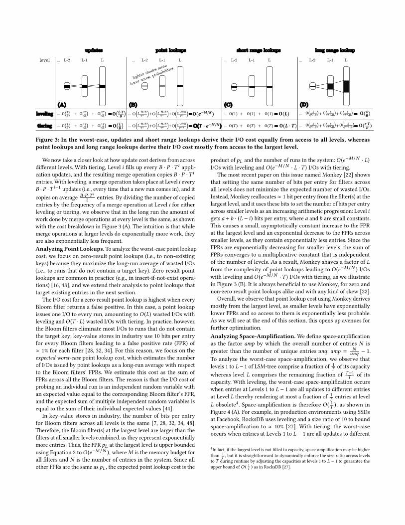
Figure 3: In the worst-case, updates and short range lookups derive their I/O cost equally from access to all levels, whereaspoint lookups and long range lookups derive their I/O cost mostly from access to the largest level.

We now take a closer look at how update cost derives from acrossdifferent levels. With tiering, Level i fills up every B · P ·T i appli-cation updates, and the resulting merge operation copies B · P ·T ientries. With leveling, a merge operation takes place at Level i everyB · P ·T i−1 updates (i.e., every time that a new run comes in), and itcopies on average B ·P ·T i

2 entries. By dividing the number of copiedentries by the frequency of a merge operation at Level i for eitherleveling or tiering, we observe that in the long run the amount ofwork done by merge operations at every level is the same, as shownwith the cost breakdown in Figure 3 (A). The intuition is that whilemerge operations at larger levels do exponentially more work, theyare also exponentially less frequent.AnalyzingPoint Lookups.To analyze theworst-case point lookupcost, we focus on zero-result point lookups (i.e., to non-existingkeys) because they maximize the long-run average of wasted I/Os(i.e., to runs that do not contain a target key). Zero-result pointlookups are common in practice (e.g., in insert-if-not-exist opera-tions) [16, 48], and we extend their analysis to point lookups thattarget existing entries in the next section.

The I/O cost for a zero-result point lookup is highest when everyBloom filter returns a false positive. In this case, a point lookupissues one I/O to every run, amounting to O (L) wasted I/Os withleveling andO (T · L) wasted I/Os with tiering. In practice, however,the Bloom filters eliminate most I/Os to runs that do not containthe target key; key-value stores in industry use 10 bits per entryfor every Bloom filters leading to a false positive rate (FPR) of≈ 1% for each filter [28, 32, 34]. For this reason, we focus on theexpected worst-case point lookup cost, which estimates the numberof I/Os issued by point lookups as a long-run average with respectto the Bloom filters’ FPRs. We estimate this cost as the sum ofFPRs across all the Bloom filters. The reason is that the I/O cost ofprobing an individual run is an independent random variable withan expected value equal to the corresponding Bloom filter’s FPR,and the expected sum of multiple independent random variables isequal to the sum of their individual expected values [44].

In key-value stores in industry, the number of bits per entryfor Bloom filters across all levels is the same [7, 28, 32, 34, 48].Therefore, the Bloom filter(s) at the largest level are larger than thefilters at all smaller levels combined, as they represent exponentiallymore entries. Thus, the FPR pL at the largest level is upper boundedusing Equation 2 toO (e−M/N ), whereM is the memory budget forall filters and N is the number of entries in the system. Since allother FPRs are the same as pL , the expected point lookup cost is the

product of pL and the number of runs in the system: O (e−M/N · L)

I/Os with leveling and O (e−M/N · L ·T ) I/Os with tiering.The most recent paper on this issue named Monkey [22] shows

that setting the same number of bits per entry for filters acrossall levels does not minimize the expected number of wasted I/Os.Instead, Monkey reallocates ≈ 1 bit per entry from the filter(s) at thelargest level, and it uses these bits to set the number of bits per entryacross smaller levels as an increasing arithmetic progression: Level igets a + b · (L − i ) bits per entry, where a and b are small constants.This causes a small, asymptotically constant increase to the FPRat the largest level and an exponential decrease to the FPRs acrosssmaller levels, as they contain exponentially less entries. Since theFPRs are exponentially decreasing for smaller levels, the sum ofFPRs converges to a multiplicative constant that is independentof the number of levels. As a result, Monkey shaves a factor of Lfrom the complexity of point lookups leading to O (e−M/N ) I/Oswith leveling and O (e−M/N ·T ) I/Os with tiering, as we illustratein Figure 3 (B). It is always beneficial to use Monkey, for zero andnon-zero result point lookups alike and with any kind of skew [22].

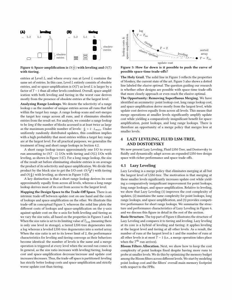
Overall, we observe that point lookup cost using Monkey derivesmostly from the largest level, as smaller levels have exponentiallylower FPRs and so access to them is exponentially less probable.As we will see at the end of this section, this opens up avenues forfurther optimization.Analyzing Space-Amplification. We define space-amplificationas the factor amp by which the overall number of entries N isgreater than the number of unique entries unq: amp = N

unq − 1.To analyze the worst-case space-amplification, we observe thatlevels 1 to L− 1 of LSM-tree comprise a fraction of 1

T of its capacitywhereas level L comprises the remaining fraction of T−1

T of itscapacity. With leveling, the worst-case space-amplification occurswhen entries at Levels 1 to L − 1 are all updates to different entriesat Level L thereby rendering at most a fraction of 1

T entries at levelL obsolete4. Space-amplification is therefore O ( 1T ), as shown inFigure 4 (A). For example, in production environments using SSDsat Facebook, RocksDB uses leveling and a size ratio of 10 to boundspace-amplification to ≈ 10% [27]. With tiering, the worst-caseoccurs when entries at Levels 1 to L − 1 are all updates to different

4In fact, if the largest level is not filled to capacity, space-amplification may be higherthan 1

T , but it is straightforward to dynamically enforce the size ratio across levelsto T during runtime by adjusting the capacities at levels 1 to L − 1 to guarantee theupper bound of O ( 1

T ) as in RocksDB [27].

leveling tiering

L-2 L-1 L L-2 L-1 L……

(A) (B)

…

……

obsolete entries

obsolete entries

Figure 4: Space-amplification isO ( 1T ) with leveling andO (T )with tiering.

entries at Level L, and where every run at Level L contains thesame set of entries. In this case, Level L entirely consists of obsoleteentries, and so space-amplification is O (T ) as level L is larger by afactor ofT − 1 than all other levels combined. Overall, space-amplif-ication with both leveling and tiering in the worst case derivesmostly from the presence of obsolete entries at the largest level.Analyzing Range Lookups. We denote the selectivity of a rangelookup s as the number of unique entries across all runs that fallwithin the target key range. A range lookup scans and sort-mergesthe target key range across all runs, and it eliminates obsoleteentries from the result set. For analysis, we consider a range lookupto be long if the number of blocks accessed is at least twice as largeas the maximum possible number of levels: s

B > 2 · Lmax . Underuniformly randomly distributed updates, this condition implieswith a high probability that most entries within a target key rangeare at the largest level. For all practical purposes, we generalize thetreatment of long and short range lookups in Section 4.2.

A short range lookup issues approximately one I/O to everyrun amounting to O (T · L) I/Os with tiering and O (L) I/Os withleveling, as shown in Figure 3 (C). For a long range lookup, the sizeof the result set before eliminating obsolete entries is on averagethe product of its selectivity and space-amplification. We divide thisproduct by the block size to get the I/O cost: O (T ·sB ) with tieringand O ( sB ) with leveling, as shown in Figure 3 (D).

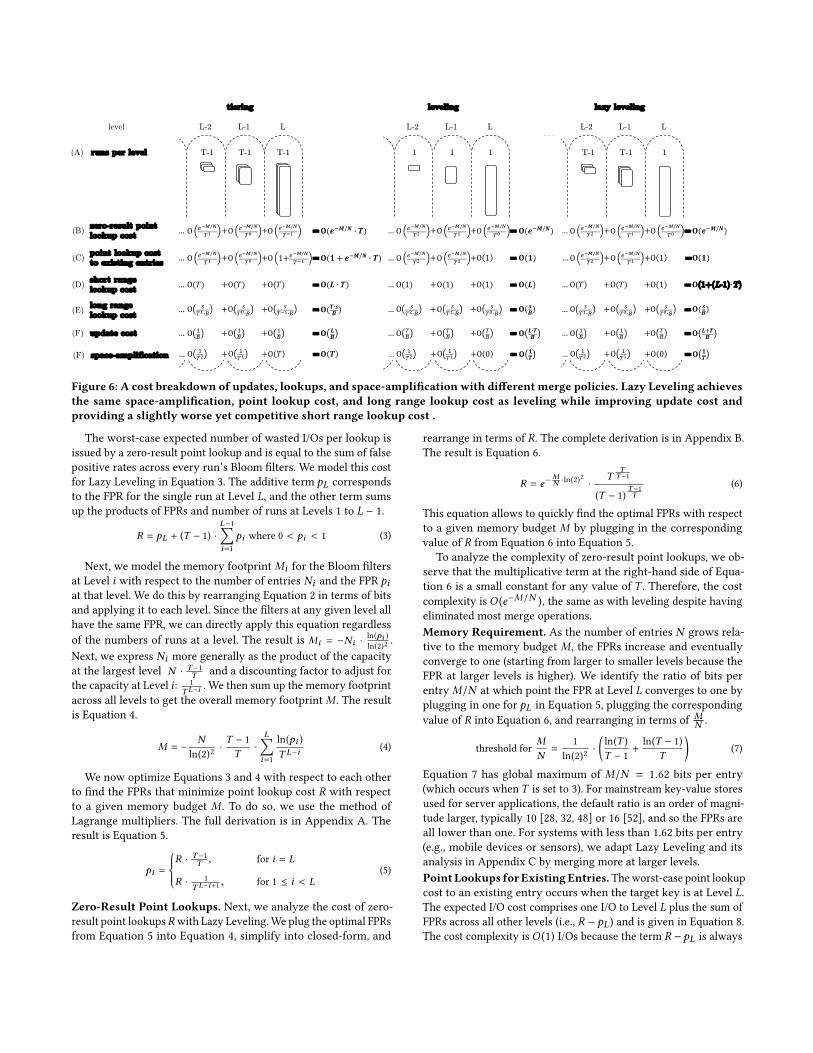
A key distinction is that a short range lookup derives its costapproximately equally from across all levels, whereas a long rangelookup derives most of its cost from access to the largest level.Mapping the Design Space to the Trade-Off Space. There is anintrinsic trade-off between update cost on one hand and the costsof lookups and space-amplification on the other. We illustrate thistrade-off in conceptual Figure 5, whereon the solid line plots thedifferent costs of lookups and space-amplification on the y-axisagainst update cost on the x-axis for both leveling and tiering aswe vary the size ratio, all based on the properties in Figures 3 and 4.When the size ratio is set to its limiting value ofTl im (meaning thereis only one level in storage), a tiered LSM-tree degenerates intoa log whereas a leveled LSM-tree degenerates into a sorted array.When the size ratio is set to its lower limit of 2, the performancecharacteristics for leveling and tiering converge as their behaviorsbecome identical: the number of levels is the same and a mergeoperation is triggered at every level when the second run comes in.In general, as the size ratio increases with leveling/tiering, lookupcost and space-amplification decrease/increase and update costincreases/decreases. Thus, the trade-off space is partitioned: levelinghas strictly better lookup costs and space-amplification and strictlyworse update cost than tiering.

look

up c

osts

&

spac

e-am

plifica

tion

update cost

log

T = 2

T = Tlim

sorted array

T = Tlim

Figure 5: How far down is it possible to push the curve ofpossible space-time trade-offs?

The Holy Grail. The solid line in Figure 5 reflects the propertiesof Monkey, the current state of the art. Figure 5 also shows a dottedline labeled the elusive optimal. The question guiding our researchis whether other designs are possible with space-time trade-offsthat more closely approach or even reach the elusive optimal.The Opportunity: Removing Superfluous Merging. We haveidentified an asymmetry: point lookup cost, long range lookup cost,and space-amplification derive mostly from the largest level, whileupdate cost derives equally from across all levels. This means thatmerge operations at smaller levels significantly amplify updatecost while yielding a comparatively insignificant benefit for space-amplification, point lookups, and long range lookups. There istherefore an opportunity of a merge policy that merges less atsmaller levels.

4 LAZY LEVELING, FLUID LSM-TREE,AND DOSTOEVSKY

We now present Lazy Leveling, Fluid LSM-Tree, and Dostoevsky tofluidly and dynamically adapt across an expanded LSM-tree designspace with richer performance and space trade-offs.

4.1 Lazy LevelingLazy Leveling is a merge policy that eliminates merging at all butthe largest level of LSM-tree. The motivation is that merging atthese smaller levels significantly increases update cost while yield-ing a comparatively insignificant improvement for point lookups,long range lookups, and space-amplification. Relative to leveling,we show that Lazy Leveling (1) improves the cost complexity ofupdates, (2) maintains the same complexity for point lookups, longrange lookups, and space-amplification, and (3) provides competi-tive performance for short range lookups. We summarize the struc-ture and performance characteristics of Lazy Leveling in Figure 6,and we discuss this figure in detail in the rest of the section.Basic Structure. The top part of Figure 6 illustrates the structure ofLazy Leveling and compares it to tiering and leveling. Lazy levelingat its core is a hybrid of leveling and tiering: it applies levelingat the largest level and tiering at all other levels. As a result, thenumber of runs at the largest level is 1 and the number of runs atall other levels is at most T − 1 (i.e., a merge operation takes placewhen the T th run arrives).Bloom Filters Allocation. Next, we show how to keep the costcomplexity of point lookups fixed despite having more runs toprobe at smaller levels.We do this by optimizing thememory budgetamong the Bloomfilters across different levels.We start bymodelingpoint lookup cost and the filters’ overall main memory footprintwith respect to the FPRs.

level L-2 L-1 L

T-1T-1T-1

tiering leveling

L-2 L-1 L

111

L-2 L-1 L

1T-1T-1

lazy leveling

+ + =… O $%O $

%O $% 𝐎 𝑳

𝑩

O(𝑇)O(𝑇)O(𝑇) 𝐎(𝑳 , 𝑻)+ + =

+ + =𝐎(𝑻,𝒔𝑩 )O /012,%O /

03,%O /02,%

…

…

+ + =… O 0%O 0

%O 0% 𝐎 𝑳,𝑻

𝑩

O(1)O(1)O(1) 𝐎(𝑳)+ + =

+ + =O /03,% 𝐎(𝒔𝑩)O /

02,%O /05,%

…

…

+ + =… O 0%O $

%O $% 𝐎 𝑳6𝑻

𝑩

+ + =O /03,% 𝐎(𝒔𝑩)O /

03,%O /02,%…

O(1)O(𝑇)O(𝑇) 𝐎(1+(L-1),T)+ + =…

update cost

short range lookup cost

long range lookup cost

(A)

+ + =… O 718/:

03 O 718/:

012O 718/:

02 𝐎(𝒆<𝑴/𝑵 , 𝑻) O 718/:

05 𝐎(𝒆<𝑴/𝑵)+ + =… O 718/:

02 O 718/:

03 O 718/:

05 𝐎(𝒆<𝑴/𝑵)+ + =O 718/:

02 O 718/:

03…zero-result point lookup cost

+ + =… O 718/:

03 O 1+718/:

012O 718/:

02 𝐎(𝟏 + 𝒆<𝑴/𝑵 , 𝑻) O 718/:

05 𝐎(𝟏)+ + =… O 718/:

02 O 1 O 718/:

05 𝐎(𝟏)+ + =O 718/:

02 O 1…point lookup cost to existing entries

runs per level

(B)

(C)

(D)

(E)

(F)

space-amplification(F) + + =… O 𝑇O $02O $

05 𝐎 𝑻 + + =… O 0O $02O $

05 𝐎 𝟏𝑻 + + =… O 0O $

02O $05 𝐎 𝟏

𝑻

Figure 6: A cost breakdown of updates, lookups, and space-amplification with different merge policies. Lazy Leveling achievesthe same space-amplification, point lookup cost, and long range lookup cost as leveling while improving update cost andproviding a slightly worse yet competitive short range lookup cost .

The worst-case expected number of wasted I/Os per lookup isissued by a zero-result point lookup and is equal to the sum of falsepositive rates across every run’s Bloom filters. We model this costfor Lazy Leveling in Equation 3. The additive term pL correspondsto the FPR for the single run at Level L, and the other term sumsup the products of FPRs and number of runs at Levels 1 to L − 1.

R = pL + (T − 1) ·L−1∑i=1

pi where 0 < pi < 1 (3)

Next, we model the memory footprintMi for the Bloom filtersat Level i with respect to the number of entries Ni and the FPR piat that level. We do this by rearranging Equation 2 in terms of bitsand applying it to each level. Since the filters at any given level allhave the same FPR, we can directly apply this equation regardlessof the numbers of runs at a level. The result is Mi = −Ni ·

ln(pi )ln(2)2 .

Next, we express Ni more generally as the product of the capacityat the largest level N · T−1T and a discounting factor to adjust forthe capacity at Level i: 1

T L−i. We then sum up the memory footprint

across all levels to get the overall memory footprintM . The resultis Equation 4.

M = −N

ln(2)2·T − 1T·

L∑i=1

ln(pi )T L−i (4)

We now optimize Equations 3 and 4 with respect to each otherto find the FPRs that minimize point lookup cost R with respectto a given memory budget M . To do so, we use the method ofLagrange multipliers. The full derivation is in Appendix A. Theresult is Equation 5.

pi =

R · T−1T , for i = L

R · 1T L−i+1

, for 1 ≤ i < L(5)

Zero-Result Point Lookups. Next, we analyze the cost of zero-result point lookupsR with Lazy Leveling.We plug the optimal FPRsfrom Equation 5 into Equation 4, simplify into closed-form, and

rearrange in terms of R. The complete derivation is in Appendix B.The result is Equation 6.

R = e−MN ·ln(2)

2·

TTT−1

(T − 1)T−1T

(6)

This equation allows to quickly find the optimal FPRs with respectto a given memory budget M by plugging in the correspondingvalue of R from Equation 6 into Equation 5.

To analyze the complexity of zero-result point lookups, we ob-serve that the multiplicative term at the right-hand side of Equa-tion 6 is a small constant for any value of T . Therefore, the costcomplexity is O (e−M/N ), the same as with leveling despite havingeliminated most merge operations.Memory Requirement. As the number of entries N grows rela-tive to the memory budget M , the FPRs increase and eventuallyconverge to one (starting from larger to smaller levels because theFPR at larger levels is higher). We identify the ratio of bits perentryM/N at which point the FPR at Level L converges to one byplugging in one for pL in Equation 5, plugging the correspondingvalue of R into Equation 6, and rearranging in terms of M

N .

threshold forMN=

1ln(2)2

·

(ln(T )

T − 1+

ln(T − 1)T

)(7)

Equation 7 has global maximum of M/N = 1.62 bits per entry(which occurs when T is set to 3). For mainstream key-value storesused for server applications, the default ratio is an order of magni-tude larger, typically 10 [28, 32, 48] or 16 [52], and so the FPRs areall lower than one. For systems with less than 1.62 bits per entry(e.g., mobile devices or sensors), we adapt Lazy Leveling and itsanalysis in Appendix C by merging more at larger levels.Point Lookups for Existing Entries.Theworst-case point lookupcost to an existing entry occurs when the target key is at Level L.The expected I/O cost comprises one I/O to Level L plus the sum ofFPRs across all other levels (i.e., R − pL) and is given in Equation 8.The cost complexity isO (1) I/Os because the term R − pL is always

poin

t lo

okup c

ost

(I/

O)

update cost (I/O)

lazy leveling

(A)

log

O!"

#/%&( )&*

O +) O +

) &,-./()&*

O1

O ()/&*

sortedarray

T = 2

T = Tlim

T = Tlim

short

range

lookup c

ost

(I/

O)

update cost (I/O)

(B)

log

leveling

O( )&*

O +) O +

) &,-./()&*

O,-. /

( )&*

O ()/&*

sortedarray

T = 2

T = Tlim

T = Tlim

lazy leveling

long r

ange

lookup c

ost

(I/

O)

update cost (I/O)

(C)

leveling

O +) O +

) &,-./()&*

O1 )

O ()/&*

sortedarray

T = 2

lazy leveling

O1

T = Tlim

logT = Tlim

O1&(

*&)/

O()&*

O1

space-a

mplifica

tion

O1

O𝑒3

4/(

O𝑒3

4/(

O+5!"

#/%&( )&*

O)&*(

Figure 7: Lazy Leveling offers better trade-offs between updates and point lookups (Part A), worse trade-offs between updatesand short range lookups (Part B), and the same trade-offs between updates and long range lookups (Part C).

less than 1 as long as the memory requirement in Equation 7 holds.

V = 1 + R − pL (8)

Range Lookups. A short range lookup issues at most O (T ) I/Osto each of the first L − 1 levels and one I/O to the largest level, andso the cost complexity is O (1 + (L − 1) · T ) I/Os. Note that thisexpression initially increases as T increases, but as T approachesits limiting value of Tl im this term converges to 1 as the additiveterm (L − 1) · T on the right-hand size becomes zero (i.e., at thispoint Lazy Leveling degenerates into a sorted array).

A long range lookup is dominated by sequential access to Level Lbecause it contains exponentially more entries than all other levels.The cost is O ( sB ) I/Os, where s is the size of the target key rangerelative to the size of the existing key space. This is the same aswith leveling despite having eliminated most merge operations.Updates.An updated entry with Lazy Leveling participates inO (1)merge operations per level across Levels 1 to L−1 and inO (T )mergeoperations at Level L. The overall number of merge operations perentry is therefore O (L +T ), and we divide it by the block size B toget the cost for a single update: O ( L+TB ). This is an improvementover the worst-case cost with leveling.Space-Amplification. In the worst case, every entry at Levels 1 toL − 1 is an update to an existing entry at Level L. Since the fractionof entries at Levels 1 to L − 1 is 1

T of the overall number of entries,space-amplification is at mostO ( 1T ). This is the same bound as withleveling despite having eliminated most merge operations.Limits. Figure 7 compares the behaviors of the different mergepolicies as we vary the size ratio T for each policy from 2 to itslimit of Tl im (i.e., at which point the number of levels drops toone). Firstly, we observe that these policies converge in terms ofperformance characteristics when the size ratioT is set to 2 becauseat this point their behaviors become identical: the number of levelsis the same and a merge operation occurs at every level when thesecond run arrives. Secondly, Part (A) of Figure 7 shows that theimprovement that Lazy Leveling achieves for update cost relativeto leveling can be traded for point lookup cost by increasing thesize ratio. This generates a new trade-off curve between updatecost and point lookup cost that dominates leveling, and convergeswith it again as T approaches Tl im (i.e., at which point both mergepolicies degenerate into a sorted array). Parts (B) shows that the

cost of small range lookups is competitive, and part (C) shows thatthis cost difference becomes negligible as the target range grows.Lesson: No Single Merge Policy Rules. Our analysis in figureFigure 7 shows that no single design dominates the others univer-sally. Lazy leveling is best for combined workloads consisting ofupdates, point lookups and long range lookups, whereas tieringand leveling are best for workloads comprising mostly updatesor mostly lookups, respectively. In the rest of the paper, we takesteps towards a unified system that adapts across these designsdepending on the application scenario.

4.2 Fluid LSM-TreeTo be able to strike all possible trade-offs for different workloads,we next introduce Fluid LSM-tree, a generalization of LSM-tree thatenables switching and combining merge policies. It does this bycontrolling the frequency of merge operations separately for thelargest level and for all other levels.Basic Structure. Figure 8 illustrates the basic structure of FluidLSM-tree. There are at mostZ runs at the largest level and at mostKruns at each of the smaller levels. To maintain these bounds, everyLevel i has an active run into which we merge incoming runs fromLevel i − 1. Each active run has a size threshold with respect to thecapacity of its level: TK percent for Levels 1 to L − 1 and T

Z percentfor Level L. When an active run reaches this threshold, we start anew active run at that level. Ultimately when a level is at capacity,all runs in it get merged and flushed down to the next level.Parameterization. The bounds K and Z are used as tuning pa-rameters that enable Fluid LSM-tree to assume the behaviors ofdifferent merge policies.

• K = 1 and Z = 1 give leveling.• K = T − 1 and Z = T − 1 give tiering.• K = T − 1 and Z = 1 give Lazy Leveling.

Fluid LSM-tree can transition from Lazy Leveling to tiering bymerging less frequently at the largest level by increasing Z , or itcan transition to leveling by merging more frequently at all otherlevels by decreasing K . Fluid LSM-tree spans all possible trade-offsalong and between the curves in Figure 7.Bloom Filters Allocation. Next, we derive the optimal FPRs thatminimize point lookup cost with respect to the parameters K and

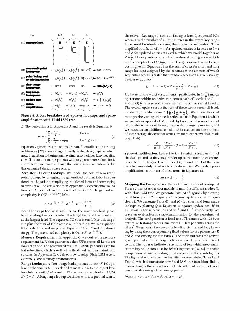
L-2 L-1 L

ZKK

+ + =… O $%&' 𝐎 𝑻

𝑩 &𝑳𝑲-

𝟏𝒁

+ + =O 1&2$3&% 𝐎(𝒔&𝒁𝑩 )O 2

$7&%O 2$8&%…

O(𝑍)O(𝐾)O(𝐾) 𝐎(Z+(L-1)&K)+ + =

𝐎(𝒁 & 𝒆<𝑴/𝑵)+ + =O @&ABCD

E&F7

…

…

level

O $%&' O $

%&1

O 1&GBCDO @&AB

CD

E&F8

𝐎(𝟏 + 𝒁 & 𝒆<𝑴/𝑵)+ + =O @&ABCD

E&F7… O(1 + 𝑍 & 𝑒<CD)O @&AB

CD

E&F8

update cost

short range lookup cost

long range lookup cost

(A)

zero-result point lookup cost

point lookup cost to existing entries

runs per level

(B)

(C)

(D)

(E)

(F)

space-amplification

(G) + + =… O J$8 O J

$ O 1<J 𝐎 𝒛 − 𝟏 + 𝟏𝑻

Figure 8: A cost breakdown of updates, lookups, and space-amplification with Fluid LSM-tree.

Z . The derivation is in Appendix A and the result is Equation 9.

pi =

RZ ·

T−1T , for i = L

RK ·

T−1T · 1

T L−i , for 1 ≤ i < L(9)

Equation 9 generalizes the optimal Bloom filters allocation strategyin Monkey [22] across a significantly wider design space, whichnow, in addition to tiering and leveling, also includes Lazy Levelingas well as custom merge policies with any parameter values for Kand Z . Next, we model and map the new space-time trade-offs thatthis expanded design space offers.Zero-Result Point Lookups. We model the cost of zero-resultpoint lookups by plugging the generalized optimal FPRs in Equa-tion 9 into Equation 4, simplifying into closed-form, and rearrangingin terms of R. The derivation is in Appendix B, experimental valida-tion is in Appendix I, and the result is Equation 10. The generalizedcomplexity is O (Z · e−M/N ) I/Os.

R = e−MN ·ln(2)

2· Z

T−1T · K

1T ·

TTT−1

T − 1(10)

Point Lookups for Existing Entries. The worst-case lookup costto an existing key occurs when the target key is at the oldest runat the largest level. The expected I/O cost is one I/O to this targetrun plus the sum of FPRs across all other runs. We use Equation8 to model this, and we plug in Equation 10 for R and Equation 9for pL . The generalized complexity is O (1 + Z · e−M/N ).Memory Requirement. In Appendix C, we derive the memoryrequirementM/N that guarantees that FPRs across all Levels arelower than one. The generalized result is 1.62 bits per entry as in thelast subsection, which is well below the default ratio in mainstreamsystems. In Appendix C, we show how to adapt Fluid LSM-tree toextremely low-memory environments.Range Lookups. A short range lookup issues at most K I/Os perlevel to the smaller L−1 Levels and at mostZ I/Os to the largest levelfor a total ofZ+K ·(L−1) random I/Os and a cost complexity ofO (Z+K · (L−1)). A long range lookup continues with a sequential scan to

the relevant key range at each run issuing at least sB sequential I/Os,

where s is the number of unique entries in the target key range.To account for obsolete entries, the number of sequential I/Os isamplified by a factor of 1+ 1

T for updated entries at Levels 1 to L−1and Z for updated entries at Level L, which we model together asZ + 1

T . The sequential scan cost is therefore at most sB · (Z +

1T ) I/Os

with a complexity of O ( s ·ZB ) I/Os. The generalized range lookupcost is given in Equation 11 as the sum of costs for short and longrange lookups weighted by the constant µ, the amount of whichsequential access is faster than random access on a given storagedevices (e.g., disk).

Q = K · (L − 1) + Z +1µ·sB·

(Z +

1T

)(11)

Updates. In the worst case, an entry participates in O ( TK ) mergeoperations within an active run across each of Levels 1 to L − 1,and in O ( TZ ) merge operations within the active run at Level L.The overall update cost is the sum of these terms across all levelsdivided by the block size: O

(TB ·

(LK +

1Z

)). We model this cost

more precisely using arithmetic series to obtain Equation 12, whichwe validate in Appendix I. We divide by the constant µ since the costof updates is incurred through sequential merge operations, andwe introduce an additional constant ϕ to account for the propertyof some storage devices that writes are more expensive than reads(e.g., flash).

W =ϕ

µ · B·

(T − 1K + 1

· (L − 1) +T − 1Z + 1

)(12)

Space-Amplification. Levels 1 to L − 1 contain a fraction of 1T of

the dataset, and so they may render up to this fraction of entriesobsolete at the largest level. In Level L, at most Z − 1 of the runsmay be completely filled with obsolete entries. We model space-amplification as the sum of these terms in Equation 13.

amp = Z − 1 +1T

(13)

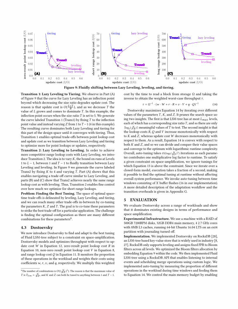
Mapping the Design Space. Figure 9 is an instance of conceptualFigure 7 that uses our cost models to map the different trade-offswith Fluid LSM-tree. We generate Part (A) of Figure 9 by plottingpoint lookup cost R in Equation 10 against update costW in Equa-tion 12. We generate Parts (B) and (C) for short and long rangelookups by plotting Q in Equation 11 against update costW inEquation 12 for selectivities s of 10−7 and 10−6, respectively. Weleave an evaluation of space-amplification for the experimentalanalysis. The configuration is fixed to a 1TB dataset with 128 byteentries, 4KB storage blocks, and overall 10 bits per entry across thefilters5. We generate the curves for leveling, tiering, and Lazy Level-ing by using their corresponding fixed values for the parameters Kand Z , and varying the size ratio T . The circle indicates the conver-gence point of all three merge policies where the size ratio T is setto two. The squares indicate a size ratio of ten, which most main-stream key-value stores use by default in practice [28, 32], to enablecomparison of corresponding points across the three sub-figures.The figure also illustrates two transition curves labeled Trans1 andTrans2, which demonstrate how Fluid LSM-tree transitions fluidlyacross designs thereby achieving trade-offs that would not havebeen possible using a fixed merge policy.5We set N = 233, E = 27, B = 25 , and M = 10 · 233 .

0.0

0.01

0.02

0.03

0.04

0.05

0.06

0.07

zero

-resu

ltpoin

tlo

okup

cost

(I/O

)

0.0 0.1 0.2 0.3 0.4 0.5 0.6

update cost (I/O)

(A)

0

10

20

30

40

50

60

70

short

range

lookup

cost

(I/O

)

0.0 0.1 0.2 0.3 0.4 0.5 0.6

update cost (I/O)

(B)

0

100

200

300

400

500

600

700

long

range

lookup

cost

(I/O

)

0.0 0.1 0.2 0.3 0.4 0.5 0.6

update cost (I/O)

(C)

leveling

tiering

lazy leveling

Trans1

tiering lazy leveling

leveling

tiering lazy leveling

levelingTrans2

Trans2

Trans1Trans2

Trans1

(A) (B) (C)

Figure 9: Fluidly shifting between Lazy Leveling, leveling, and tiering.

Transition 1: Lazy Leveling to Tiering.We observe in Part (A)of Figure 9 that the curve for Lazy Leveling has an inflection pointbeyond which decreasing the size ratio degrades update cost. Thereason is that update cost is O ( L+TB ), and as we decrease T thevalue of L grows and comes to dominate T . In this example, theinflection point occurs when the size ratioT is set to 5. We generatethe curve labeled Transition 1 (Trans1) by fixing T to the inflectionpoint value and instead varyingZ from 1 toT −1 (4 in this example).The resulting curve dominates both Lazy Leveling and tiering forthis part of the design space until it converges with tiering. Thus,Transition 1 enables optimal trade-offs between point lookup costand update cost as we transition between Lazy Leveling and tieringto optimize more for point lookups or updates, respectively.Transition 2: Lazy Leveling to Leveling. In order to achievemore competitive range lookup costs with Lazy Leveling, we intro-duce Transition 2. The idea is to varyK , the bound on runs at Levels1 to L − 1, between 1 and T − 1 to fluidly transition between LazyLeveling and leveling. In Figure 9 we generate the curve labeledTrans2 by fixing K to 4 and varying T . Part (A) shows that thisenables navigating a trade-off curve similar to Lazy Leveling, andparts (B) and (C) show that Trans2 achieves nearly the same rangelookup cost as with leveling. Thus, Transition 2 enables fine controlover how much we optimize for short range lookups.Problem: Finding the Best Tuning. The space of optimal space-time trade-offs is delineated by leveling, Lazy Leveling, and tiering,and we can reach many other trade-offs in-between by co-tuningthe parameters K , Z andT . The goal is to co-tune these parametersto strike the best trade-off for a particular application. The challengeis finding the optimal configuration as there are many differentcombinations for these parameters6.

4.3 DostoevskyWe now introduce Dostoevsky to find and adapt to the best tuningof Fluid LSM-tree subject to a constraint on space-amplification.Dostoevsky models and optimizes throughput with respect to up-date cost W in Equation 12, zero-result point lookup cost R inEquation 10, non-zero result point lookup cost V in Equation 8,and range lookup costQ in Equation 11. It monitors the proportionof these operations in the workload and weights their costs usingcoefficientsw , r , v , and q, respectively. We multiply this weighted

6The number of combinations isO (( NB ·P )3 ). The reason is that the maximum value of

T is Tl im = NB ·P , and K and Z can both be tuned to anything between 1 and T − 1.

cost by the time to read a block from storage Ω and taking theinverse to obtain the weighted worst-case throughput τ .

τ = Ω−1 · (w ·W + r · R + v · V + q ·Q )−1 (14)

Dostoevsky maximizes Equation 14 by iterating over differentvalues of the parameters T , K , and Z . It prunes the search space us-ing two insights. The first is that LSM-tree has at most Lmax levels,each of which has a corresponding size ratioT , and so there are only⌈log2 (

NP ·B )⌉ meaningful values ofT to test. The second insight is that

the lookup costs R, Q and V increase monotonically with respectto K and Z , whereas update costW decreases monotonically withrespect to them. As a result, Equation 14 is convex with respect toboth K and Z , and so we can divide and conquer their value spacesand converge to the optimum with logarithmic runtime complexity.Overall, auto-tuning takes O (loд2 ( N

B ·P )3 ) iterations as each parame-ter contributes one multiplicative log factor to runtime. To satisfya given constraint on space-amplification, we ignore tunings forwhich Equation 13 is above the constraint. Since we iterate over aclosed-form model, execution takes a fraction of a second, makingit possible to find the optimal tuning at runtime without affectingoverall system performance. We invoke auto-tuning between timewindows consisting of X buffer flushes (16 in our implementation).A more detailed description of the adaptation workflow and thetransition overheads is given in Appendix G.

5 EVALUATIONWe evaluate Dostoevsky across a range of workloads and showthat it dominates existing designs in terms of performance andspace-amplification.Experimental Infrastructure.We use a machine with a RAID of500GB 7200RPM disks, 32GB DDR4 main memory, 4 2.7 GHz coreswith 8MB L3 caches, running 64-bit Ubuntu 16.04 LTS on an ext4partition with journaling turned off.Implementation. We implemented Dostoevsky on RocksDB [28],an LSM-tree based key-value store that is widely used in industry [8,27]. RocksDB only supports leveling and assigns fixed FPR to Bloomfilters across all levels. We optimized the Bloom filters allocation byembedding Equation 9 within the code. We then implemented FluidLSM-tree using a RocksDB API that enables listening to internalevents and scheduling merge operations using custom logic. Weimplemented auto-tuning by measuring the proportion of differentoperations in the workload during time windows and feeding themto Equation 14. We control the main memory budget by enabling

10,9,9

10,5,9

10,4,9

8,3,7

5,1,4

5,1,4

4,1,3

5,1,4

7,1,6

8,1,7

10,1,9

15,1,14

20,1,10

50,1,10

T,Z,K

10,1,9

T,Z,K

10,1,9

10,1,9

10,1,9

10,1,9

10,1,9

10,1,4

6,1,9

10,1,1

30,1,1

100,1,1

0.0

0.1

0.2

0.3

0.4

0.5

0.6

0.7

0.8

0.9

1.0

norm

alize

dth

roughput

(ops/

s)

102 101

(A) point lookups / updates

0

0.5

1

norm

alize

dth

roughput

(ops/

s)

102 101

(B) point lookups / updates

ParametersK: bound on runs at Levels 1 to L 1Z: bound on runs at Level LT : size ratio

SystemsDostoevskyMonkeyWell-Tuned RocksDBDefault RocksDB

Existing Design SpaceTiering (T = 10)Leveling (T = 10)

Fluid LSM-Tree New Design SpaceTransition 1 (T = 10, Z = 4, K = 9)Lazy Leveling (T = 10)Transition 2 (T = 10, Z = 1, K = 4)

0.0

0.2

0.4

0.6

0.8

1.0

1.2

zero

-res

poin

tlo

okup

late

ncy

(ms)

0.0 0.00225 0.0045 0.00675 0.009

(C) update latency (ms)

64 TB16 TB1 TB

0.001

0.0015

0.002

0.0025

0.003

0.0035

0.004

0.0045

0.005

0.0055

0.006

update

late

ncy

(ms)

0.1 0.2 0.3 0.4 0.5 0.6 0.7 0.8 0.9

(D) skew coecient

0

10

20

30

40

50

60

70

80

90

exis

ting

poin

tlo

okup

late

ncy

(ms)

1 2 3 4 5 6 7 8 9 10

(E) bits per element

0

20

40

60

80

100

space

-am

plifica

tion

(%)

0 0.2 0.4 0.6 0.8 1

(F) updates / insertions

0.0

0.1

0.2

0.3

0.4

0.5

0.6

0.7

0.8

0.9

1.0

norm

alize

dra

nge

lookup

late

ncy

109 108 107 106 105 104 103 102

(G) range lookup selectivity (%)

0

0.5

1

norm

alize

dth

roughput

(ops/

s)

109108107106105104103102

(H) short range lookups / (updates & point)

Figure 10: Dostoevsky dominates existing designs by being able to strike better space-time trade-offs.

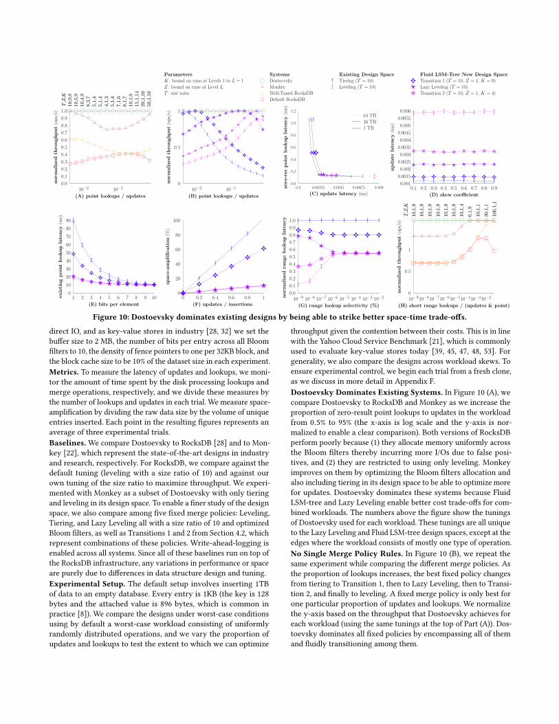
direct IO, and as key-value stores in industry [28, 32] we set thebuffer size to 2 MB, the number of bits per entry across all Bloomfilters to 10, the density of fence pointers to one per 32KB block, andthe block cache size to be 10% of the dataset size in each experiment.Metrics. To measure the latency of updates and lookups, we moni-tor the amount of time spent by the disk processing lookups andmerge operations, respectively, and we divide these measures bythe number of lookups and updates in each trial. We measure space-amplification by dividing the raw data size by the volume of uniqueentries inserted. Each point in the resulting figures represents anaverage of three experimental trials.Baselines. We compare Dostoevsky to RocksDB [28] and to Mon-key [22], which represent the state-of-the-art designs in industryand research, respectively. For RocksDB, we compare against thedefault tuning (leveling with a size ratio of 10) and against ourown tuning of the size ratio to maximize throughput. We experi-mented with Monkey as a subset of Dostoevsky with only tieringand leveling in its design space. To enable a finer study of the designspace, we also compare among five fixed merge policies: Leveling,Tiering, and Lazy Leveling all with a size ratio of 10 and optimizedBloom filters, as well as Transitions 1 and 2 from Section 4.2, whichrepresent combinations of these policies. Write-ahead-logging isenabled across all systems. Since all of these baselines run on top ofthe RocksDB infrastructure, any variations in performance or spaceare purely due to differences in data structure design and tuning.Experimental Setup. The default setup involves inserting 1TBof data to an empty database. Every entry is 1KB (the key is 128bytes and the attached value is 896 bytes, which is common inpractice [8]). We compare the designs under worst-case conditionsusing by default a worst-case workload consisting of uniformlyrandomly distributed operations, and we vary the proportion ofupdates and lookups to test the extent to which we can optimize

throughput given the contention between their costs. This is in linewith the Yahoo Cloud Service Benchmark [21], which is commonlyused to evaluate key-value stores today [39, 45, 47, 48, 53]. Forgenerality, we also compare the designs across workload skews. Toensure experimental control, we begin each trial from a fresh clone,as we discuss in more detail in Appendix F.Dostoevsky Dominates Existing Systems. In Figure 10 (A), wecompare Dostoevsky to RocksDB and Monkey as we increase theproportion of zero-result point lookups to updates in the workloadfrom 0.5% to 95% (the x-axis is log scale and the y-axis is nor-malized to enable a clear comparison). Both versions of RocksDBperform poorly because (1) they allocate memory uniformly acrossthe Bloom filters thereby incurring more I/Os due to false posi-tives, and (2) they are restricted to using only leveling. Monkeyimproves on them by optimizing the Bloom filters allocation andalso including tiering in its design space to be able to optimize morefor updates. Dostoevsky dominates these systems because FluidLSM-tree and Lazy Leveling enable better cost trade-offs for com-bined workloads. The numbers above the figure show the tuningsof Dostoevsky used for each workload. These tunings are all uniqueto the Lazy Leveling and Fluid LSM-tree design spaces, except at theedges where the workload consists of mostly one type of operation.No Single Merge Policy Rules. In Figure 10 (B), we repeat thesame experiment while comparing the different merge policies. Asthe proportion of lookups increases, the best fixed policy changesfrom tiering to Transition 1, then to Lazy Leveling, then to Transi-tion 2, and finally to leveling. A fixed merge policy is only best forone particular proportion of updates and lookups. We normalizethe y-axis based on the throughput that Dostoevsky achieves foreach workload (using the same tunings at the top of Part (A)). Dos-toevsky dominates all fixed policies by encompassing all of themand fluidly transitioning among them.

Dostoevsky is More Scalable. In Figure 10 (C), we compare LazyLeveling to the other merge policies as we increase the data size.Point lookup cost does not increase as the data size grows becausewe scale the Bloom filters’ memory budget in proportion to the datasize. The first takeaway is that Lazy Leveling achieves the samepoint lookup cost as leveling while significantly reducing updatecost by eliminating most merge operations. The second takeawayis that update cost with Lazy Leveling scales at a slower rate thanwith leveling as the data size increases because it merges greedilyonly at the largest level even as the number of levels grows. As aresult, Dostoevsky offers increasingly better performance relativeto state-of-the-art designs as the data size grows.

Robust Update Improvement Across Skews. In Figure 10 (D),we evaluate the different fixed merge policies under a skewed up-date pattern. We vary a skew coefficient whereby a fraction of c ofall updates target a fraction of 1 − c of the most recently updatedentries. The flat lines show that update cost is largely insensitive toskew with all merge policies. The reason is that levels in LSM-treegrow exponentially in size, and so even an update to the most recent10% of the data traverses all levels rather than getting eliminatedprematurely while getting merged across smaller levels. Hence, theimproved update cost offered by Lazy Leveling and by Dostoevskyby extension is robust across a wide range of temporal update skews.We experiment with point lookup skews in Appendix H.

Robust Performance Across Memory Budgets. In Figure 10(E), we vary the memory budget allocated to the Bloom filters andwe measure point lookup latency to existing entries. Even withas little as one bit per entry, Lazy Leveling achieves comparablelatency to leveling, and so Dostoevsky achieves robust point lookupperformance across a wide range of memory budgets.

Lower Space-Amplification. In Figure 10 (F), we vary the pro-portion of updates of existing entries to insertions of new entries,and we measure space-amplification. As the proportion of updatesincreases, there are more obsolete entries at larger levels, and sospace-amplification increases. We observe that space-amplificationfor Lazy Leveling and Leveling increase at the same rate, despiteeliminating most merge operations. As a result, Dostoevsky is ableto achieve a given bound on space-amplification while paying alower toll in terms of update cost due to merging.

DominationwithRange Lookups. Figure 10 (G) compares rangelookup costs as selectivity increases. The first takeaway is that forlow selectivities, Transition 2 achieves a competitive short rangelookup cost with leveling while achieving comparable bounds onpoint lookups and space-amplification (as showed in Figures 10(C), (E) and (F), respectively). The second takeaway is that as selec-tivity increases Lazy Leveling becomes increasingly competitive.We demonstrate how Dostoevsky uses these designs in Figure 10(H), where we increase the proportion of short range lookups inthe workload while keeping a fixed ratio of five updates per pointlookup. The best fixed merge policy changes from Lazy Levelingto Transition 2 to Leveling as the proportion of range lookupsincreases. Dostoevsky transitions among these policies therebymaximizing throughput and dominating existing systems.

6 RELATEDWORKKey-Value Stores in Industry. Mainstream key-value stores inindustry [6, 19, 28, 31, 32, 34, 48, 52] have the same architecture asDostoevsky: they persist data using LSM-tree and speed up pointlookups using Bloom filters. However, they are tuned suboptimallyover a small subset of the design space. LevelDB [32] hard codesthe size ratio to 10 and the merge policy to leveling. RocksDB [28]supports leveling but not tiering. bLSM [48] restricts the numberof levels to 3 by merging more aggressively as data grows. None ofthese systems optimize memory allocation across the Bloom filtersto minimize point lookup cost. Overall, it is hard to tune thesesystems even within their limited design spaces as the impact ofany existing tuning parameter on performance is unclear.Key-Value Stores in Research. Key-value stores in research ex-pand the trade-offs that are possible to achieve and navigate. Somedesigns use fractional cascading [13, 35] rather than fence point-ers thereby trading lookup cost for memory. Bϵ -tree and variants[2, 15, 42] use buffered in-place updates among linked nodes in-stead of fence pointers thereby trading memory for space and rangelookup cost, as nodes are padded and non-contiguous. Other de-signs [4, 11, 24, 25] use circular logs in storage and index themusing a hash table in memory thereby trading space for updatecost. Recent work [36] optimizes the size ratio of leveled LSM-treefor update skew. PebblesDB [45] merges more frequently acrossfrequently accessed parts of the key space. Monkey [22] allocatesmain memory among the Bloom filters of LSM-tree to minimizepoint lookup cost, and it transitions between leveling and tieringto maximize throughput.Dostoevsky. Our insight is that the recent Bloom filters optimiza-tion in Monkey [22] offers a new avenue for optimizing update costby relaxing merging at lower levels while keeping point lookupcost fixed. We exploit this by introducing Lazy Leveling, whichoffers better scalability trade-offs among point lookups, long rangelookups, updates, and space-amplification than we knew existedbefore. We further introduce Fluid LSM-Tree and Dostoevsky togeneralize and be able to navigate the expanded design space.Related Topics. In Appendix E, we discuss complementary tech-niques for reducing and scheduling merge operations. We alsodiscuss specialized and in-memory key-value stores.

7 CONCLUSIONWe show that merges in LSM-tree based key-value stores controlan intrinsic trade-off among the costs of updates, point lookups,range lookups, and space-amplification, yet existing designs donot strike optimal trade-offs among these metrics. The reason isthat merge operations do the same amount of maintenance workacross all levels, yet point lookups, long range lookups, and space-amplification derive their cost mostly from the largest level. Weintroduce Dostoevsky, a key-value store that offers richer space-time trade-offs by merging as little as possible to achieve givenbounds on lookup cost and space, and we show how to find thebest trade-off for a particular application workload and hardware.

Acknowledgments.We thank the anonymous reviewers for theirvaluable feedback. This work is supported by the National ScienceFoundation under grant IIS-1452595.

REFERENCES[1] A. Aggarwal and J. S. Vitter. The Input/Output Complexity of Sorting and Related

Problems. Communications of the ACM, 31(9):1116–1127, 1988.[2] D. Agrawal, D. Ganesan, R. Sitaraman, Y. Diao, and S. Singh. Lazy-Adaptive

Tree: An Optimized Index Structure for Flash Devices. Proceedings of the VLDBEndowment, 2(1):361–372, 2009.

[3] M. Y. Ahmad and B. Kemme. Compaction management in distributed key-valuedatastores. Proceedings of the VLDB Endowment, 8(8):850–861, 2015.

[4] D. G. Andersen, J. Franklin, M. Kaminsky, A. Phanishayee, L. Tan, and V. Va-sudevan. FAWN: A Fast Array of Wimpy Nodes. In Proceedings of the ACMSymposium on Operating Systems Principles (SOSP), pages 1–14, 2009.

[5] Apache. Accumulo. https://accumulo.apache.org/, 2016.[6] Apache. Cassandra. http://cassandra.apache.org, 2016.[7] Apache. HBase. http://hbase.apache.org/, 2016.[8] T. G. Armstrong, V. Ponnekanti, D. Borthakur, and M. Callaghan. LinkBench: a

Database Benchmark Based on the Facebook Social Graph. In Proceedings of theACM SIGMOD International Conference on Management of Data, pages 1185–1196,2013.

[9] M. Athanassoulis, S. Chen, A. Ailamaki, P. B. Gibbons, and R. Stoica. MaSM:Efficient Online Updates in Data Warehouses. In Proceedings of the ACM SIGMODInternational Conference on Management of Data, pages 865–876, 2011.

[10] M. Athanassoulis, S. Chen, A. Ailamaki, P. B. Gibbons, and R. Stoica. OnlineUpdates on Data Warehouses via Judicious Use of Solid-State Storage. ACMTransactions on Database Systems (TODS), 40(1), 2015.

[11] A. Badam, K. Park, V. S. Pai, and L. L. Peterson. HashCache: Cache Storage forthe Next Billion. In Proceedings of the USENIX Symposium on Networked SystemsDesign and Implementation (NSDI), pages 123–136, 2009.

[12] O. Balmau, D. Didona, R. Guerraoui, W. Zwaenepoel, H. Yuan, A. Arora, K. Gupta,and P. Konka. TRIAD: Creating synergies between memory, disk and log in logstructured key-value stores. In USENIX Annual Technical Conference, 2017.

[13] M. A. Bender, M. Farach-Colton, J. T. Fineman, Y. R. Fogel, B. C. Kuszmaul, andJ. Nelson. Cache-Oblivious Streaming B-trees. In Proceedings of the Annual ACMSymposium on Parallel Algorithms and Architectures (SPAA), pages 81–92, 2007.

[14] B. H. Bloom. Space/Time Trade-offs in Hash Coding with Allowable Errors.Communications of the ACM, 13(7):422–426, 1970.

[15] G. S. Brodal and R. Fagerberg. Lower Bounds for ExternalMemoryDictionaries. InProceedings of the Annual ACM-SIAM Symposium on Discrete Algorithms (SODA),pages 546–554, 2003.

[16] N. G. Bronson, Z. Amsden, G. Cabrera, P. Chakka, P. Dimov, H. Ding, J. Ferris,A. Giardullo, S. Kulkarni, H. C. Li, M. Marchukov, D. Petrov, L. Puzar, Y. J. Song,and V. Venkataramani. TAO: Facebook’s Distributed Data Store for the SocialGraph. In Proceedings of the USENIX Annual Technical Conference (ATC), pages49–60, 2013.

[17] Y. Bu, V. Borkar, J. Jia, M. J. Carey, and Condie. Pregelix: Big (ger) graph analyticson a dataflow engine. In Proceedings of the International Conference on Very LargeData Bases (VLDB), pages 161–172, 2014.

[18] Z. Cao, S. Chen, F. Li, M. Wang, and X. S. Wang. LogKV: Exploiting Key-ValueStores for Log Processing. In Proceedings of the Biennial Conference on InnovativeData Systems Research (CIDR), 2013.

[19] F. Chang, J. Dean, S. Ghemawat, W. C. Hsieh, D. A. Wallach, M. Burrows, T. Chan-dra, A. Fikes, and R. E. Gruber. Bigtable: A Distributed Storage System forStructured Data. In Proceedings of the USENIX Symposium on Operating SystemsDesign and Implementation (OSDI), pages 205–218, 2006.

[20] J. Chen, C. Douglas, M. Mutsuzaki, P. Quaid, R. Ramakrishnan, S. Rao, andR. Sears. Walnut: A Unified Cloud Object Store. In Proceedings of the ACMSIGMOD International Conference on Management of Data, pages 743–754, 2012.

[21] B. F. Cooper, A. Silberstein, E. Tam, R. Ramakrishnan, and R. Sears. Benchmarkingcloud serving systems with YCSB. In Proceedings of the ACM Symposium on CloudComputing (SoCC), pages 143–154, 2010.

[22] N. Dayan, M. Athanassoulis, and S. Idreos. Monkey: Optimal Navigable Key-Value Store. In Proceedings of the ACM SIGMOD International Conference onManagement of Data, pages 79–94, 2017.

[23] N. Dayan, P. Bonnet, and S. Idreos. GeckoFTL: Scalable Flash Translation Tech-niques For Very Large Flash Devices. In Proceedings of the ACM SIGMOD Inter-national Conference on Management of Data, pages 327–342, 2016.

[24] B. Debnath, S. Sengupta, and J. Li. FlashStore: high throughput persistent key-value store. Proceedings of the VLDB Endowment, 3(1-2):1414–1425, 2010.

[25] B. Debnath, S. Sengupta, and J. Li. SkimpyStash: RAM space skimpy key-valuestore on flash-based storage. In Proceedings of the ACM SIGMOD InternationalConference on Management of Data, pages 25–36, 2011.

[26] G. DeCandia, D. Hastorun, M. Jampani, G. Kakulapati, A. Lakshman, A. Pilchin,S. Sivasubramanian, P. Vosshall, and W. Vogels. Dynamo: Amazon’s HighlyAvailable Key-value Store. ACM SIGOPS Operating Systems Review, 41(6):205–220,2007.

[27] S. Dong, M. Callaghan, L. Galanis, D. Borthakur, T. Savor, and M. Strum. Optimiz-ing Space Amplification in RocksDB. In Proceedings of the Biennial Conference onInnovative Data Systems Research (CIDR), 2017.

[28] Facebook. RocksDB. https://github.com/facebook/rocksdb, 2016.

[29] Facebook. MyRocks. http://myrocks.io/, 2017.[30] B. Fitzpatrick and A. Vorobey. Memcached: a distributed memory object caching

system, 2011.[31] G. Golan-Gueta, E. Bortnikov, E. Hillel, and I. Keidar. Scaling Concurrent Log-

Structured Data Stores. In Proceedings of the ACM European Conference onComputer Systems (EuroSys), pages 32:1—-32:14, 2015.

[32] Google. LevelDB. https://github.com/google/leveldb/, 2016.[33] H. V. Jagadish, P. P. S. Narayan, S. Seshadri, S. Sudarshan, and R. Kanneganti.

Incremental Organization for Data Recording and Warehousing. In Proceedingsof the International Conference on Very Large Data Bases (VLDB), pages 16–25,1997.

[34] A. Lakshman and P. Malik. Cassandra - A Decentralized Structured StorageSystem. ACM SIGOPS Operating Systems Review, 44(2):35–40, 2010.

[35] Y. Li, B. He, J. Yang, Q. Luo, K. Yi, and R. J. Yang. Tree Indexing on Solid StateDrives. Proceedings of the VLDB Endowment, 3(1-2):1195–1206, 2010.

[36] H. Lim, D. G. Andersen, and M. Kaminsky. Towards Accurate and Fast Evaluationof Multi-Stage Log-structured Designs. In Proceedings of the USENIX Conferenceon File and Storage Technologies (FAST), pages 149–166, 2016.

[37] H. Lim, B. Fan, D. G. Andersen, and M. Kaminsky. SILT: A Memory-Efficient,High-Performance Key-Value Store. In Proceedings of the ACM Symposium onOperating Systems Principles (SOSP), pages 1–13, 2011.

[38] LinkedIn. Online reference. http://www.project-voldemort.com, 2016.[39] L. Lu, T. S. Pillai, A. C. Arpaci-Dusseau, and R. H. Arpaci-Dusseau. WiscKey:

Separating Keys from Values in SSD-conscious Storage. In Proceedings of theUSENIX Conference on File and Storage Technologies (FAST), pages 133–148, 2016.

[40] S. Nath and A. Kansal. FlashDB: dynamic self-tuning database for NAND flash.ACM/IEEE IPSN, 2007.

[41] P. E. O’Neil, E. Cheng, D. Gawlick, and E. J. O’Neil. The log-structured merge-tree(LSM-tree). Acta Informatica, 33(4):351–385, 1996.

[42] A. Papagiannis, G. Saloustros, P. González-Férez, and A. Bilas. Tucana: Design andImplementation of a Fast and Efficient Scale-up Key-value Store. In Proceedingsof the USENIX Annual Technical Conference (ATC), pages 537–550, 2016.

[43] M. Pilman, K. Bocksrocker, L. Braun, R. Marroquin, and D. Kossmann. Fast Scanson Key-Value Stores. Proceedings of the VLDB Endowment, 10(11):1526–1537,2017.

[44] J. Pitman. Probability. 1999.[45] P. Raju, R. Kadekodi, V. Chidambaram, and I. Abraham. Pebblesdb: Building

key-value stores using fragmented log-structured merge trees. Proceedings of theACM Symposium on Operating Systems Principles, 2017.

[46] Redis. Online reference. http://redis.io/.[47] K. Ren, Q. Zheng, J. Arulraj, and G. Gibson. SlimDB: A Space-Efficient Key-

Value Storage Engine For Semi-Sorted Data. Proceedings of the VLDB Endowment,10(13):2037–2048, 2017.

[48] R. Sears and R. Ramakrishnan. bLSM: A General Purpose Log Structured MergeTree. In Proceedings of the ACM SIGMOD International Conference on Managementof Data, pages 217–228, 2012.

[49] P. Shetty, R. P. Spillane, R. Malpani, B. Andrews, J. Seyster, and E. Zadok. BuildingWorkload-Independent Storage with VT-trees. In Proceedings of the USENIXConference on File and Storage Technologies (FAST), pages 17–30, 2013.

[50] S. Tarkoma, C. E. Rothenberg, and E. Lagerspetz. Theory and Practice of Bloom Fil-ters for Distributed Systems. IEEE Communications Serveys & Tutorials, 14(1):131–155, 2012.

[51] R. Thonangi and J. Yang. On Log-Structured Merge for Solid-State Drives. InProceedings of the IEEE International Conference on Data Engineering (ICDE), pages683–694, 2017.

[52] WiredTiger. WiredTiger. https://github.com/wiredtiger/wiredtiger, 2016.[53] X. Wu, Y. Xu, Z. Shao, and S. Jiang. LSM-trie: An LSM-tree-based Ultra-Large

Key-Value Store for Small Data Items. In Proceedings of the USENIX AnnualTechnical Conference (ATC), pages 71–82, 2015.

A OPTIMAL FALSE POSITIVE RATESIn this appendix, we derive the optimal false positive rates (FPRs)for Fluid LSM-tree that minimize the zero-result point lookup cost.This result can then be applied to any particular merge policy byplugging in the appropriate parameters K and Z . First, we modelpoint lookup cost with respect to these parameters:

R = Z · pL + K ·L−1∑i=1

pi (15)

Next, we use the method of Lagrange multipliers to find the FPRsthat minimize Equation 4 subject to Equation 15 as a constraint.We first express these in the standard form:

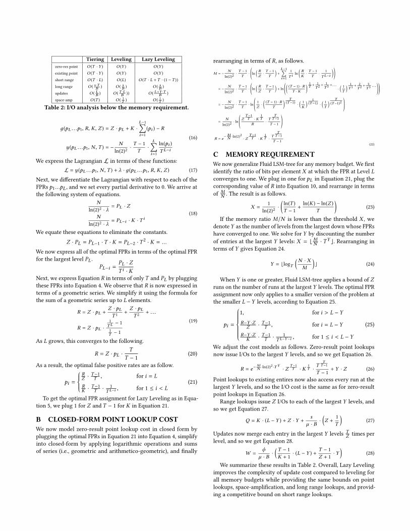
Tiering Leveling Lazy Levelingzero-res point O (T · Y ) O (Y ) O (Y )

existing point O (T · Y ) O (Y ) O (Y )

short range O (T · L) O (L) O (T · L +T · (1 −T ))

long range O ( s ·TB ) O ( sB ) O ( sB )

updates O ( LB ) O ( T ·LB )) O ( L+Y ·TB )

space-amp O (T ) O ( 1T ) O ( 1T )

Table 2: I/O analysis below the memory requirement.

д (pL ...p1, R, K, Z ) = Z · pL + K ·L−1∑i=1

(pi ) − R

y (pL ...p1, N , T ) = −N

ln(2)2·T − 1T·

L∑i=1

ln(pi )T L−i

(16)

We express the Lagrangian L in terms of these functions:L = y (pL ...p1, N , T ) + λ · д (pL ...p1, R, K, Z ) (17)

Next, we differentiate the Lagrangian with respect to each of theFPRs p1...pL , and we set every partial derivative to 0. We arrive atthe following system of equations.

Nln(2)2 · λ

= PL · Z

Nln(2)2 · λ

= PL−i · K · T i(18)

We equate these equations to eliminate the constants.

Z · PL = PL−1 ·T · K = PL−2 ·T2 · K = ...

We now express all of the optimal FPRs in terms of the optimal FPRfor the largest level PL .

PL−i =PL · Z

T i · KNext, we express Equation R in terms of onlyT and PL by pluggingthese FPRs into Equation 4. We observe that R is now expressed interms of a geometric series. We simplify it using the formula forthe sum of a geometric series up to L elements.

R = Z · pL +Z · pLT 1 +

Z · pLT 2 + ...

R = Z · pL ·1T L− 1

1T − 1

(19)

As L grows, this converges to the following.

R = Z · pL ·T

T − 1(20)

As a result, the optimal false positive rates are as follow.

pi =

RZ ·

T−1T , for i = L

RK ·

T−1T · 1

T L−i , for 1 ≤ i < L(21)

To get the optimal FPR assignment for Lazy Leveling as in Equa-tion 5, we plug 1 for Z and T − 1 for K in Equation 21.

B CLOSED-FORM POINT LOOKUP COSTWe now model zero-result point lookup cost in closed form byplugging the optimal FPRs in Equation 21 into Equation 4, simplifyinto closed-form by applying logarithmic operations and sumsof series (i.e., geometric and arithmetico-geometric), and finally

rearranging in terms of R, as follows.

M = −N

ln(2)2·T − 1T

·*.,ln

( RZ·T − 1T

)+

L−1∑i=1

1T i

ln(RK·T − 1T

·1

T L−i

)+/-

= −N

ln(2)2·T − 1T

·*.,ln

( RZ·T − 1T

)+ ln *.

,

((T − 1) · RT · K

) 1T +

1T 2 +

1T 3 +. . .

·

( 1T

) 1T 1 +

2T 2 +

3T 3 . . . +/

-

+/-

= −N

ln(2)2·T − 1T

· ln*..,

1Z·

((T − 1) · R

T

) T(T−1)

·

( 1K

) 1(T−1) ·

( 1T

) T(T−1)2 +//

-

=N

ln(2)2· ln

*..,

ZT−1T · K

1T

R·T

TT−1T − 1

+//-

R = e−MN ·ln(2)

2· Z

T−1T · K

1T ·

TTT−1T − 1

(22)

C MEMORY REQUIREMENTWe now generalize Fluid LSM-tree for any memory budget. We firstidentify the ratio of bits per element X at which the FPR at Level Lconverges to one. We plug in one for pL in Equation 21, plug thecorresponding value of R into Equation 10, and rearrange in termsof M

N . The result is as follows.

X =1

ln(2)2·

(ln(T )

T − 1+

ln(K ) − ln(Z )

T

)(23)

If the memory ratio M/N is lower than the threshold X , wedenoteY as the number of levels from the largest down whose FPRshave converged to one. We solve for Y by discounting the numberof entries at the largest Y levels: X = ⌊MN · T

Y ⌋. Rearranging interms of Y gives Equation 24.

Y = ⌊logT(N · X

M

)⌋ (24)

When Y is one or greater, Fluid LSM-tree applies a bound of Zruns on the number of runs at the largest Y levels. The optimal FPRassignment now only applies to a smaller version of the problem atthe smaller L − Y levels, according to Equation 25.

pi =

1, for i > L − Y

R−Y ·ZZ · T−1T , for i = L − Y

R−Y ·ZK · T−1T · 1

T L−Y−i , for 1 ≤ i < L − Y

(25)

We adjust the cost models as follows. Zero-result point lookupsnow issue I/Os to the largest Y levels, and so we get Equation 26.

R = e−MN ·ln(2)

2 ·TY· Z

T−1T · K

1T ·

TTT−1

T − 1+ Y · Z (26)

Point lookups to existing entires now also access every run at thelargest Y levels, and so the I/O cost is the same as for zero-resultpoint lookups in Equation 26.

Range lookups issue Z I/Os to each of the largest Y levels, andso we get Equation 27.

Q = K · (L − Y ) + Z · Y +s

µ · B·

(Z +

1T

)(27)

Updates now merge each entry in the largest Y levels TZ times per

level, and so we get Equation 28.

W =ϕ

µ · B·

(T − 1K + 1

· (L − Y ) +T − 1Z + 1

· Y)

(28)

We summarize these results in Table 2. Overall, Lazy Levelingimproves the complexity of update cost compared to leveling forall memory budgets while providing the same bounds on pointlookups, space-amplification, and long range lookups, and provid-ing a competitive bound on short range lookups.

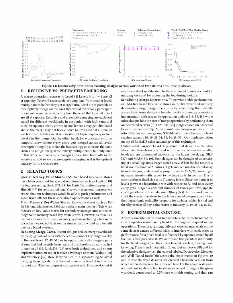
10,9,9

10,5,9

10,4,9

8,3,7

5,1,4

5,1,4

4,1,3

5,1,4

7,1,6

8,1,7

10,1,9

15,1,14

20,1,10

50,1,10

T,Z,K

0.0

0.1

0.2

0.3

0.4

0.5

0.6

0.7

0.8

0.9

1.0

transi

tion

cost

(dat

afr

acti

onre

wri

tten

)

102 101

(A) point lookups / updates

0.0

0.1

0.2

0.3

0.4

0.5

0.6

0.7

0.8

0.9

1.0

norm

alize

dth

roughput

(ops/

sec)

102 101

(B) point lookups / updates

ParametersK: bound on runs at Levels 1 to L 1Z: bound on runs at Level LT : size ratio

SystemsDostoevskyMonkey

Existing Design SpaceTiering (T = 10)Leveling (T = 10)

Fluid LSM-Tree New Design SpaceTransition 1 (T = 10, Z = 4, K = 9)Lazy Leveling (T = 10)Transition 2 (T = 10, Z = 1, K = 4)

0

2

4

6

8

10

12

poin

tlo

okup

late

ncy

(ms)

0.1 0.2 0.3 0.4 0.5 0.6 0.7 0.8 0.9

(C) skew coecient

0.0

0.02

0.04

0.06

0.08

0.1

0.12

poin

tlo

okup

cost

(I/O

)

0.1 0.2 0.3 0.4 0.5 0.6 0.7

(D) update cost (I/O)

Experimental ResultModel

Figure 11: Dostoevsky dominates existing designs across workload transitions and lookup skews.D RECURSIVE VS. PREEMPTIVE MERGINGA merge operation recurses to Level i if Levels 0 to i − 1 are allat capacity. To avoid recursively copying data from smaller levelsmultiple times before they get merged into Level i , it is possible topreemptively merge all the runs that would eventually participatein a recursive merge by detecting from the onset that Levels 0 to i−1are all at capacity. Recursive and preemptive merging are each bestsuited for different workloads. In particular, with high temporalskew for updates, many entries in smaller runs may get eliminatedand so the merge may not trickle down to level i even if all smallerlevels are full. In this case, it is desirable not to preemptively includeLevel i in the merge. On the other hand, for workloads with notemporal skew where every entry gets merged across all levels,preemptive merging is in fact the best strategy as it means the sameentries do not get merged recursively multiple times but only once.In this work, our concern is managing space-time trade-offs in theworst-case, and so we use preemptive merging as it is the optimalstrategy for the worst-case.

E RELATED TOPICSSpecialized Key-Value Stores. LSM-tree based Key-value storeshave been proposed for specialized domains such as LogKB [18]for log processing, GeckoFTL[23] for Flash Translation Layers, andSlimDB [47] for semi-sorted data. Our work is general-purpose, weexpect that our techniques would be able to push performance andspace trade-offs for these specialized applications as well.Main Memory Key-Value Stores. Key-value stores such as Re-dis [46] and Memcached [30] store data in main memory. This workfocuses on key-value stores for secondary storage, and so it is or-thogonal to memory based key-value stores. However, as there is amemory hierarchy for main memory systems including a hierarchyof caches, we expect that such a similar study would also benefitmemory based systems.Reducing Merge Costs. Recent designs reduce merge overheadsby merging parts of runs with the least amount of key range overlapin the next level [12, 49, 51], or by opportunistically merging partsof runs that had recently been read and are therefore already cachedin memory [43]. RocksDB [28] uses both techniques, and so ourimplementation on top of it takes advantage of them. Walnut [20]and WiscKey [39] store large values in a separate log to avoidmerging them repeatedly at the cost of an extra level of indirectionfor lookups. This technique is compatible with Dostoevsky but it

requires a slight modification to the cost model to only account formerging keys and for accessing the log during lookups.Scheduling Merge Operations. To provide stable performance,all LSM-tree based key-value stores in the literature and industryde-amortize large merge operations by scheduling them evenlyacross time. Some designs schedule fractions of merge operationsincrementally with respect to application updates [13, 35, 48], whileother designs hide the cost of merge operations by performing themon dedicated servers [3]. LSM-trie [53] merges based on hashes ofkeys to restrict overlap. Most mainstream designs partition runsinto SSTables and merge one SSTable at a time whenever a levelreaches capacity [6, 19, 28, 31, 32, 34, 48, 52]. Our implementationon top of RocksDB takes advantage of this technique.Unbounded Largest Level. Log-structured designs in the liter-ature have have been proposed with fixed capacities for smallerlevels and an unbounded capacity for the largest level, e.g., SILT[37] and MASM [9, 10]. Such designs can be thought of as consist-ing of a small log and a larger sorted array. When the log reaches afixed size threshold ofX entries, it gets merged into the sorted array.In such designs, update cost is proportional toO (N /X ), meaning itincreases linearly with respect to the data size N . In contrast, Dosto-evsky enforces fixed size ratioT among levels. Since the number oflevels grows at a logarithmic rate with respect to N , and since everyentry gets merged a constant number of times per level, updatecost logarithmic in the data size: O (logT (N )). In this work, we re-strict the scope of analysis to the latter class of designs due to theirtheir logarithmic scalability property for updates, which is vital andthereby used in all key-value stores in industry [7, 19, 28, 34, 48, 52].

F EXPERIMENTAL CONTROLAny experimentation on LSM-trees is subject to the problem that thecost of updates is not paid upfront but through subsequent mergeoperations. Therefore, running different experimental trials on thesame dataset causes different trials to interfere with each other asperformance for a given trial is influenced by updates issued by allthe trials that preceded it. We addressed this problem differentlyfor the fixed designs (i.e., the curves labeled Leveling, Tiering, LazyLeveling, Transition 1, Transition 2, and Default RocksDB) and forthe adaptive designs (i.e., the curved labeled Dostoevsky, Monkey,and Well-Tuned RocksDB) across the experiments in Figures 10and 11. For the fixed designs, we created a baseline version fromwhichwe created a new clone for each trial. For the adaptive designs,we used cost models to find in advance the best tuning for the givenworkload, constructed an LSM-tree with this tuning, and then ran

the experiment on it. Starting from a brand new LSM-tree for eachtrial eliminated interference among the trials thereby ensuringexperimental control. Another positive feature of this approachis that it enforced experimental control by isolating the study ofdifferent designs from the study of how to transition among them(which is an issue we now explain separately in Appendix G).

G DYNAMIC RUNTIME ADAPTATIONAdaptation in Dostoevsky consists of three phases: Measurement,Computation, and Transition. In Section 4.3, we focused on theComputation Phase. We now fill in the details and evaluate thewhole adaptation workflow.Measurement Phase. The Measurement Phase in Dostoevsky isresponsible for workload detection through time windows. Thelength of a window is a multiple of X buffer flushes during whichwe count the number of different operations in the workload andthe average selectivities of range lookups. X is a parameter thatcontrols a trade-off between the speed vs. the accuracy of findingthe best tuning. In our implementation we set X to 16 by default,though it is possible to alleviate the trade-off between speed vs.accuracy through known smoothing techniques across the timewindows [2, 40]. This phase involves no I/O, and so it does notcontribute significantly to overall system overheads.Computation Phase. At the end of the Measurement Phase, werun the Computation Phase to find the optimal tuning of FluidLSM-tree given the workload statistics. We describe the algorithmand its runtime characteristics in Section 4.3. In practice, runtimetakes up a fraction of a second and involves no I/O, and so thisphase does not contribute significantly to system overheads.Transition Phase. The Transition Phase physically adapts FluidLSM-tree to the new target tuning found by the Computation Phase.Our transition strategy reconciles for the fact that the I/O costof lookups is paid immediately whereas the I/O cost of updatesis paid later through merge operations. It does this by adaptinglazily or greedily depending on whether the new target tuning ismore update-optimized or lookup-optimized relative to the currenttuning, respectively. If the target tuning is more update-optimized,we adapt lazily by relaxing the merge policy so that the amortizedcost of updates through subsequentmerge operations is reduced. Onthe other hand, if the new target tuning is more lookup-optimized,we trigger merge operations greedily so that subsequent lookupsbecome cheaper as quickly as possible.

Figure 11 (A) and (B) compare transition costs between Dosto-evsky and Monkey across designs that are optimized for differentworkloads. The values on top of Figure 11 (A) for the parameters T ,K , and Z reflect the optimal tunings used by Dostoevsky earlier forthe experiment in Figure 10 (A) in Section 5, where we evaluatedthese designs independently of transition overheads. We now factorin transition overheads to show their impact on throughput. Onthe y-axis in Figure 10 (A), we measure the pure transition costof Dostoevsky between adjacent designs in terms of the fractionof the overall data that was rewritten while transitioning. Despitesome peaks, Dostoevsky merges 28% less than Monkey across alltransitions (i.e., measured by the sizes of the areas underneath thecurves). The reason is that Dostoevsky adapts across designs thatare more similar to each other (i.e., Transition 2, Lazy Leveling,

and Transition 1), whereas Monkey transitions across designs thatare comparatively more different. In other words, the Dostoevskydesign space is more dense and so optimal designs for similar work-loads are structurally closer to each other and require less of atransition overhead. In Figure 10 (B), we show how transition over-heads impact throughput. For each of these trials, we started withthe structure represented by the previous point, transitioned to thenew tuning, and continued to run the workload for a combined Nupdate/lookup operations. We measure overall throughput includ-ing the time taken for transitions. Dostoevsky largely outperformsMonkey across the board because it offers more highly optimizeddesigns for individual workloads as well as lower transition over-heads across these designs. In fact, had we continued to run theworkload for longer in each of these trials, the curves will haveeventually converged to the ones in Figure 10 (A) as the transitioncosts become increasingly amortized during a stable workload.

Greedy transitioning for optimizing lookups is a single point inthe space of possible policies. Future work directions include piggy-backing transitions on regular merge operations to amortize tran-sition costs, and scheduling transitions more cautiously to ensurethat workload periodicity and volatility do not turn transitions intopure overhead. This topic deserves a much larger study, whereasthe current adaptive policies are a starting point to demonstratethat the design space is worth navigating.

H ROBUST POINT LOOKUP PERFORMANCEACROSS SKEWS

In Figure 11 (C), we verify that our experimental results generalizeacross a wide range of lookup skews. In the experiment, a fractionof c of the lookups target the least recently inserted fraction of 1−cof the entries. The horizontal lines show that point lookup cost isinsensitive to skew across all designs. The intuition is that mostof the data is at the largest level and so most lookups that targetrecently inserted entries still reach the largest level most of thetime. As a result, the models that Dostoevsky uses to transitionacross designs are robust across workload skews.

I MODEL VALIDATIONIn Figure 11 (D), we validate our I/O cost models against the exper-imental results. We created this figure by comparing the number ofI/Os per operation that we observe in practice vs. the number ofI/Os predicted by our cost models in Section 4.2. Every point alongthe line labeled Experimental Result is the average taken from thou-sands of updates and lookups. As shown, the experimental resultshave a slightly higher update cost than predicted by our model.The reason is that our model does not take account of I/Os issuedby writing to RocksDB’s log. Moreover, the experimental resultshave a slightly lower zero-result point lookup cost. The reasonis that runs in RocksDB are partitioned and merged as units ofSSTables. When an SSTable is merged into the next level, it leavesa hole in the key-space at its origin level [51]. RocksDB is aware ofsuch holes by maintaining the first and last key of every SSTablein main memory, and so it eliminates the chance of a false positiveby avoiding access to the level altogether if the target key targets akey range for which there is a hole. Despite these sources of error,our model provides a good fit for the experimental results.