Dose-Response Modeling for EPA’s Organophosphate CumulativeRisk Assessment: Combining

Information from Several Datasets toEstimate Relative Potency Factors

R. Woodrow SetzerNational Center for Computational Toxicology

Office of Research and DevelopmentU.S. Environmental Protection Agency

Background

• Food Quality Protection Act, 1996Requires EPA to take into account when setting pesticide tolerances

“available evidence concerning the cumulative effects on infants and children of such residues and other substances that have a common mechanism of toxicity.”

Cumulative Risk (per FQPA):

• The risk associated with concurrent exposure by all relevant pathways & routes of exposure to a group of chemicals that share a common mechanism of toxicity.

Identifying the Common Mechanism Group: OP

Pesticides

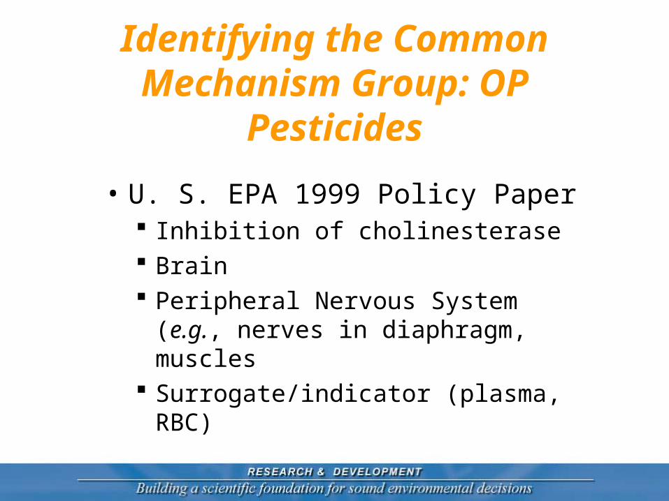
• U. S. EPA 1999 Policy Paper Inhibition of cholinesterase Brain Peripheral Nervous System (e.g.,

nerves in diaphragm, muscles Surrogate/indicator (plasma, RBC)

Synergy?

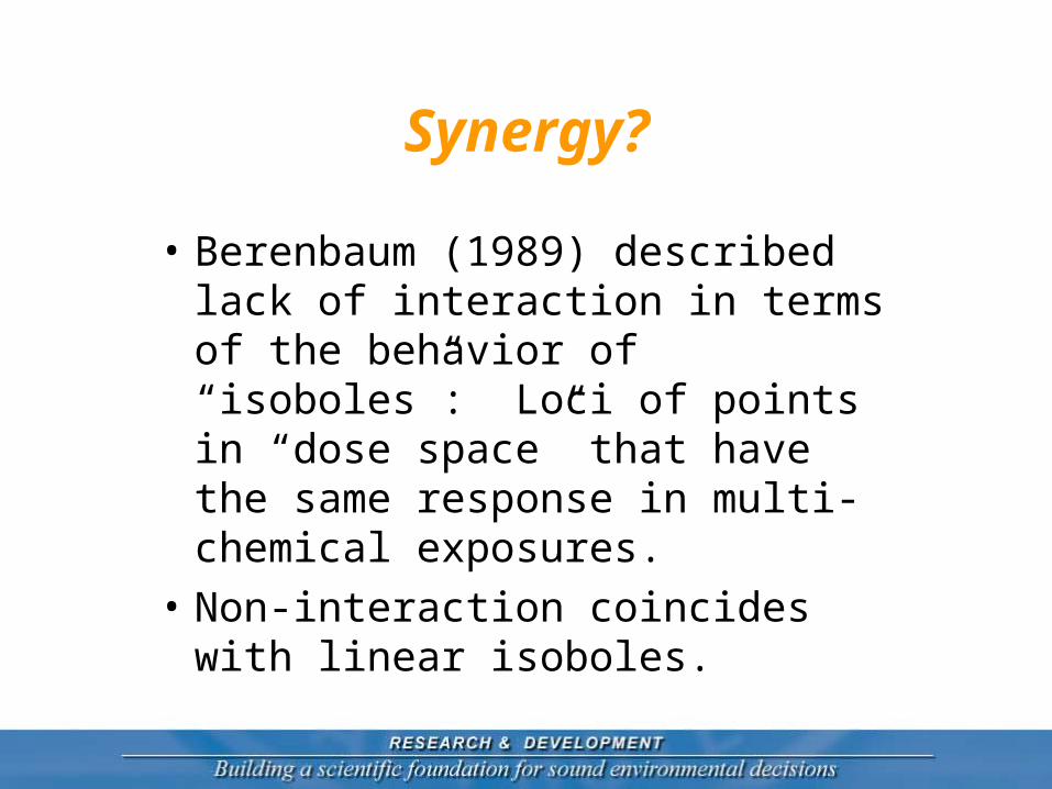
• Berenbaum (1989) described lack of interaction in terms of the behavior of “isoboles”: Loci of points in “dose space” that have the same response in multi-chemical exposures.

• Non-interaction coincides with linear isoboles.

Isoboles Example: 2 chems

Dose Chem 1

Dos

e C

hem

2

Dose-Response for Non-Interactive Mixture

For a two-chemical mixture, (d1, d2),

if D1 is the dose of chem 1 that gives response R, D2 is the dose of chem 2 that gives response R, then all the mixtures that give response R satisfy the equation:

1 2

1 2

1d d

D D

1

1

1n

n

dd

D D

For n chemicals:

:line

:hyperplane

Special Case

• When fi(x) = f(ki x): chemicals in a mixture act as if they were dilutions of each other Isoboles are linear and parallel Dose-response function for mixture is

f(k1x1+k2x2) Typically, pick one chemical as index (say

1 here) and express others in terms of that.

Then RPF for 2 is k2/k1

Strategy of Assessment

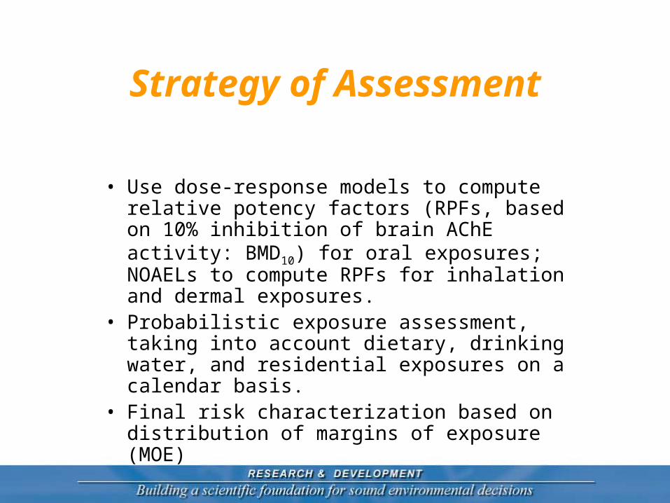
• Use dose-response models to compute relative potency factors (RPFs, based on 10% inhibition of brain AChE activity: BMD10) for oral exposures; NOAELs to compute RPFs for inhalation and dermal exposures.

• Probabilistic exposure assessment, taking into account dietary, drinking water, and residential exposures on a calendar basis.

• Final risk characterization based on distribution of margins of exposure (MOE)

OP CRA Science Team

• Vicki Dellarco • Elizabeth Doyle • Jeff Evans• David Hrdy• Anna Lowit• David Miller• Kathy Monk • Steve Nako

• Stephanie Padilla

• Randolph Perfetti • William O. Smith • Nelson Thurman • William Wooge• Plus Many, Many

Others

Oral Dose-Response Data

• Brain acetylcholinesterase (AChE) (as well as plasma and RBC)

• Female and male rats• Subchronic and chronic feeding bioassays• Always multiple studies for compounds• Often multiple assay methods• Ultimately, 33 OPs included• Usually ~ 10 animals per dose group/sex• Control CVs < 10%

Database of Acetylcholine Esterase

Data• 33 chemicals• 80+single-chemical studies• 3 compartments (brain, rbc, plasma)

2 sexes• multiple durations of exposure,

subchronic to chronic• total >1655 dose-response relationships

(~ 1300 retained)

Data StructureChemical

Study 1 Study 3Study 2

MF M MF F(in each Study X Sex) Mean, SD, N

Doses Compart. DS1 DS2 DS3 DS4

1

Brain X X X X

RBC X X X X

Plasma X X X X

… … … … … …

k

Brain X X X X

RBC X X X X

Plasma X X X X

Experimental Design

Chemical

Study 1 Study 3Study 2

MF M MF F

(in each StudyXSex:)

Doses Animals Compart. DS1 DS2 DS3 DS4

Di

1

Brain X

RBC X X

Plasma X X

… … … … … …

n

Brain X

RBC X X

Plasma X X

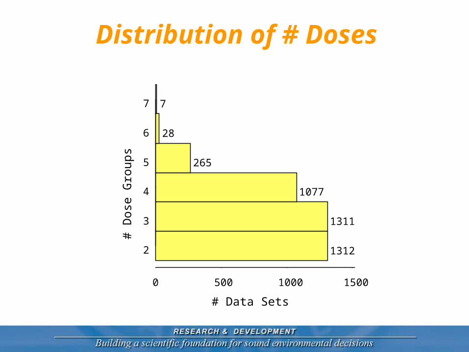
Distribution of # Doses

2

3

4

5

6

7

# Data Sets

# D

ose

Gro

ups

0 500 1000 1500

1312

1311

1077

265

28

7

Exposure Duration

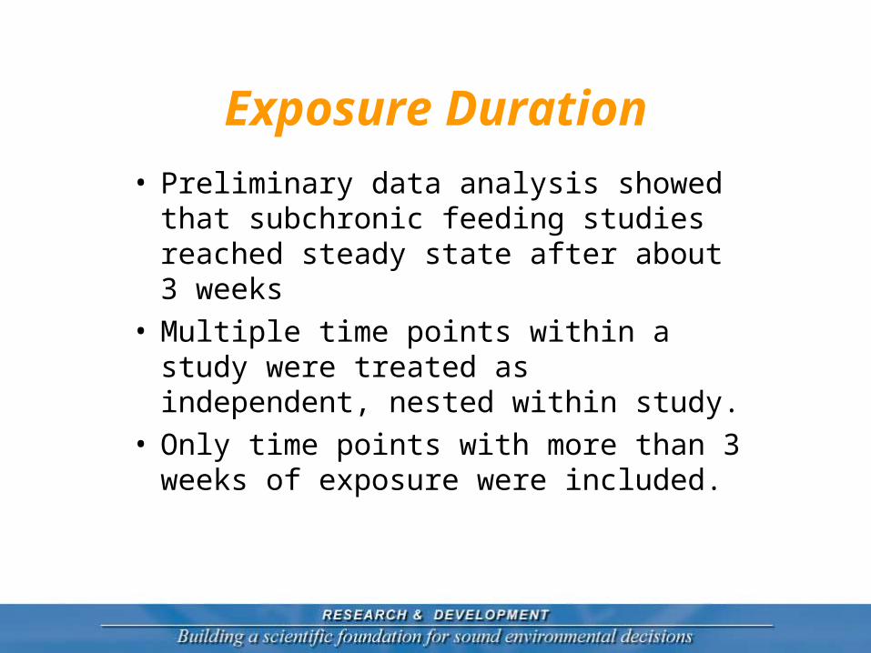
• Preliminary data analysis showed that subchronic feeding studies reached steady state after about 3 weeks

• Multiple time points within a study were treated as independent, nested within study.

• Only time points with more than 3 weeks of exposure were included.

Issues for Modeling

• Use as much of the acceptable data as possible

• Different units/analytic methods used• Expect responses to differ among

compartments, maybe sexes• Generally small number of dose levels

in a single data set (limiting the number of parameters that can be identified)

Hierarchical Structure of BMD Estimate

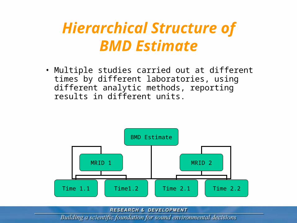
• Multiple studies carried out at different times by different laboratories, using different analytic methods, reporting results in different units.

BMD Estimate

MRID 1 MRID 2

Time 1.1 Time1.2 Time 2.1 Time 2.2

Two Modeling Approaches:

1. Model individual data sets, combining estimates.

2. Model the combined studies for each chemical compartment. Combined estimate is the estimate of the mean parameter (current revised risk assessment).

Modeling Individual Datasets

• Fit a model to each dataset, estimating BMD (and estimated standard error) each time.

• Model all three compartments and both sexes

• Use the global two-stage method (Davidian and Giltinan, 1995; 138-142) twice, once for each level of variability.

Dose-Response and Potency: Approach 1

15000 500 1000

050

010

0015

0020

00

Dose

AC

hE A

ctiv

ity

exp

1 e m

lm Dose

B By A P P

potency

Sequential Approach to Fitting

• Fit full model to all data using generalized nonlinear least squares (gnls)

• If no convergence or inadequate fit, Repeat (until good fit or # remaining doses

< 3):• set PB 0

• refit to dataset• drop highest dose

Potency Measure• Absolute potency is BMD calculated from fitted

model:

• Relative Potency:

• IF PBI = PBk

0.9ln

1Bk

Bkk

k

PP

BMDm

10.9ln 110.9ln 1

BIBII kI

k IBk

Bk k

PPBMD mm

BMD mPP m

Estimate dose-response for each dataset:

Random Effects Model for BMD

• Log(BMD) = μlBMD+ EMRID + ETime in MRID

• μlBMD varies between sexes• EMRID ~ N(0,σMRID

2)• ETime in MRID ~ N(0,σTiM

2)• Error variance proportional to (predicted)

mean of AChE activity at that dose; constant of proportionality varied among MRIDs.

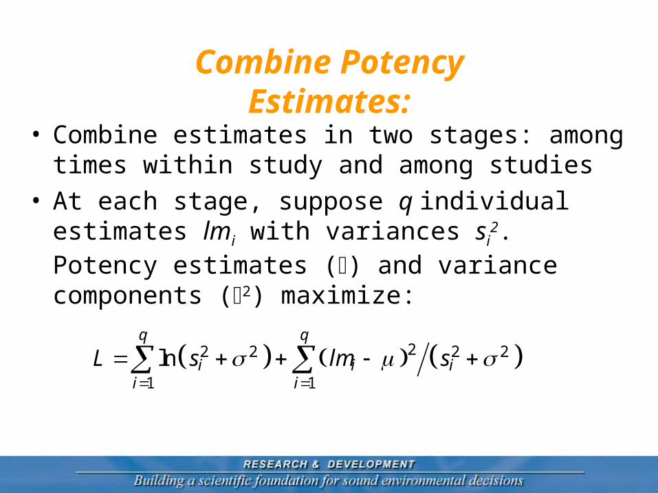
Combine Potency Estimates:

• Combine estimates in two stages: among times within study and among studies

• At each stage, suppose q individual estimates lmi with variances si

2. Potency estimates () and variance components (2) maximize:

22 2 2 2

1 1

lnq q

i i ii i

L s lm s

Combine Potency (more)• Variances for ln(potency) estimates:

• This implements the ‘Global Two-Stage’ method of Davidian and Giltinan, (1995)

• This method could apply to any single statistic or parameter, or vector statistic with simple modification.

2 21

1

1q

i is

Problems

• Estimate of m depends on PB. Particularly a problem when we cannot estimate PB.

• Would like a formal test of whether PBs differ among chemicals.

• Is there a shoulder on the dose-response curve in the low-dose region?

Solution

• Fit the same model to multiple related datasets, allowing information about DR shape to be shared across datasets

• Develop a more elaborate model that takes into account some of the biology to give a better description of the lower dose behavior.

Stage 1: A simple PBPK Model

Body ( C b)

Liver ( C l)

Metabolism ( V max , K m )

Urine ( ke)

Ingestion (Dose ×BW/24)

Q b

Q l

C a

• Two compartments: Liver and everything else.

• Oral dosing, assume 100% into the portal circulation

• Only consider saturable metabolic clearance and first order renal clearance.

• Run to steady state

Stage 1 (more)• Solve the system of differential equations

implied by the model for steady state. • The concentration of non-metabolized parent

OP in the body (idose) as a function of administered oral Dose rate is:

2

max

0.5 *

4

24 24;l b m e

l e b e l b

idose Dose S D

Dose S D Dose S

QQ K k VS D

BW Q k Q k QQ BW

Stage 2: Same as Before

• But reparametrized:

1log

1

1 e

B

B

m

P BMR

Pidose

iBMD

B By A P P

DR with First Pass Metabolism

0 2 4 6 8 10

0

500

1000

1500

2000

Dose

0

2

4

6

8

10

Sca

led

Inte

rna

l Do

se

AC

hE A

ctiv

ity

S =20.20.001

D = 2

Hierarchical Model:

• All datasets for a chemical fitted jointly using nlme in R.

• S and D varied only among chemicals

• A varied among sex × data set

• PB varied between sexes

• BMD random (same model as before)

Dose Response

0.0 0.4 0.8 1.2

0

5

10

15

Dose (mg/kg/day)

AC

hE

(U

/G)

Benchmark Dose: Fitting One Dataset at a Time

0.01 0.10 1.00

BMD

M

F

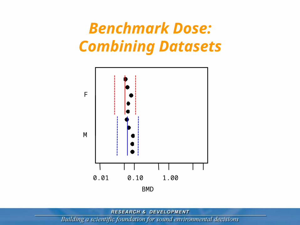
Benchmark Dose: Combining Datasets

0.01 0.10 1.00

BMD

M

F

0.0 0.2 0.4 0.6 0.8

-10

-5

0

5

Inhibition

Re

sid

ua

ls

Overall Quality of Fit: Residuals

Re

lati

ve

Po

ten

cy

0.001

0.01

0.1

1M

ALA

THIO

N

TE

TR

AC

HLO

RV

INP

HO

S

BE

NS

ULI

DE

TR

ICH

LOR

FO

N

PR

OFE

NO

FO

S

CH

LOR

PY

RIP

HO

SM

ET

HY

L

PH

OS

ALO

NE

DIA

ZIN

ON

TR

IBU

FO

SP

HO

SM

ET

DIC

HLO

RV

OS

PIR

IMIP

HO

SM

ET

HY

L

FE

NA

MIP

HO

S

CH

LOR

PY

RIF

OS

ETH

OP

RO

P

FO

ST

HIA

ZA

TE

NA

LED

AC

EP

HA

TE

AZI

NP

HO

SM

ET

HY

L

ME

TH

YLP

AR

ATH

ION

CH

LOR

ETH

OX

YF

OS

PH

OS

TE

BU

PIR

IM

ME

TH

IDA

TH

ION

DIM

ET

HO

AT

EF

EN

TH

ION

PH

OR

AT

E

ME

VIN

PH

OS

TE

RB

UF

OS

OX

YD

EM

ET

ON

ME

TH

YL

OM

ET

HO

AT

E

ME

TH

AM

IDO

PH

OS

DIS

ULF

OT

ON

DIC

RO

TOP

HO

S

Relative Potencies

Computing a MOE (Margin of Exposure)

Chem RPFExposure

(μg/kg/day)Eq.

Exposure

A (Index) 1.00 0.2 0.2

B 0.1 1.0 0.1

C 1.2 0.2 0.24

Total Equivalent Exposure 0.54

BMD10(A) = 0.08 mg/kg/day

MOE = 0.08 X 1000 μg/kg/day / 0.54 = 148

Distribution of Total MOEs

1. Combining Estimates

• Keeps dose-response modeling “simple”

• Delays problems about heterogeneity (sexes, compartments, studies, etc.) until after the modeling.

• Number of dose levels in the “smallest” dataset limits the model used, have to drop data sets with too few doses for the selected model.

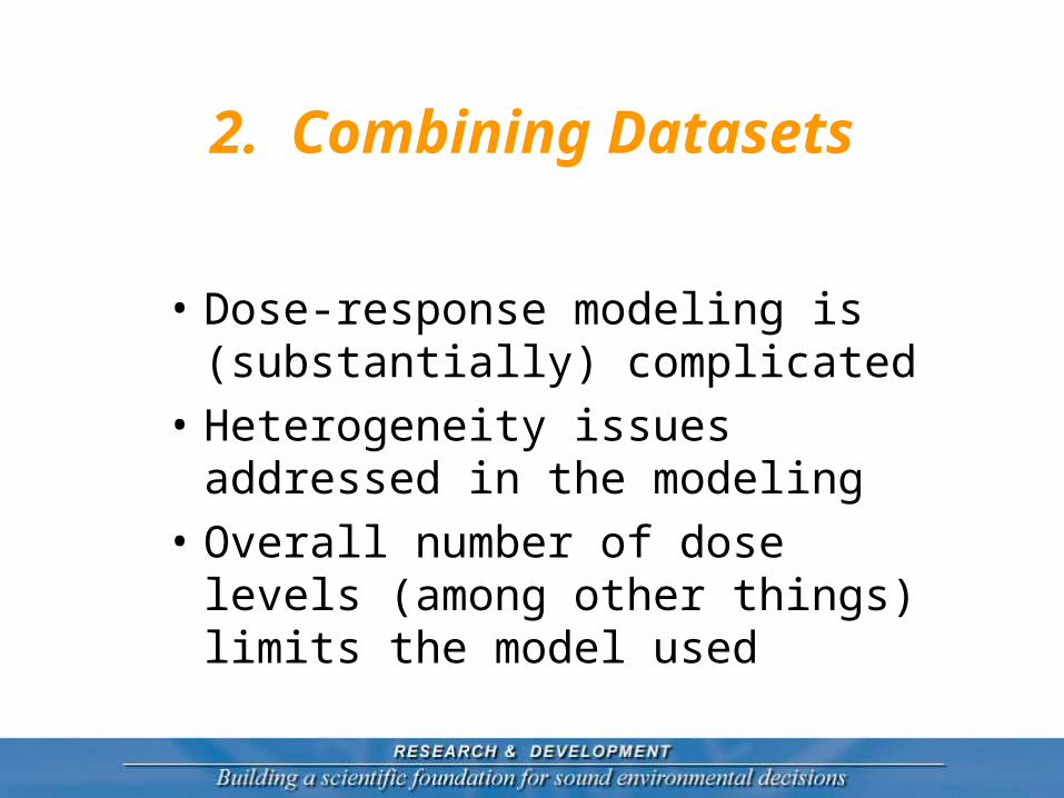
2. Combining Datasets

• Dose-response modeling is (substantially) complicated

• Heterogeneity issues addressed in the modeling

• Overall number of dose levels (among other things) limits the model used

Is PB a High-Dose Effect?

• Maybe, but could also be a consequence of multiple binding sites with different functions, or other aspects of the kinetics of AChE inhibition such as variation in aging among chemicals, which could manifest effects at lower doses as well.

Horizontal Asymptotes

0.0

0.2

0.4

0.6

0.8

FO

ST

HIA

ZA

TE

TR

IBU

FO

S

DIC

HLO

RV

OS

DIC

RO

TO

PH

OS

ME

TH

AM

IDO

PH

OS

OX

YD

EM

ET

ON

ME

TH

YL

TE

TR

AC

HLO

RV

INP

HO

S

NA

LED

ET

HO

PR

OP

AC

EP

HA

TE

FE

NA

MIP

HO

S

TR

ICH

LOR

FO

N

PH

OR

AT

E

ME

TH

YLP

AR

AT

HIO

N

BE

NS

ULI

DE

MA

LAT

HIO

N

TE

RB

UF

OS

AZ

INP

HO

SM

ET

HY

L

PH

OS

ALO

NE

PH

OS

ME

T

FE

NT

HIO

N

DIS

ULF

OT

ON

CH

LOR

PY

RIF

OS

ME

TH

IDA

TH

ION

ME

VIN

PH

OS

DIM

ET

HO

AT

E

PIR

IMIP

HO

SM

ET

HY

L

DIA

ZIN

ON

CH

LOR

PY

RIP

HO

SM

ET

HY

L

Direct Acting Require Activation

PB

Should We Expect Dose-Additivity? (Not Exactly!)

• Low-dose shoulder significantly improves fit in a substantial number of chemicals. At best, expect dose-additivity in terms of target dose.

• Horizontal asymptotes differ significantly among chemicals (P << 10-6), so dose-additivity cannot hold exactly.

Beginnings of A Theoretical Approach

• Through mathematical analysis and in silico experiments, ask: What features determine the shape

of individual chemical dose-response curves, and

what are the features of chemicals (if any) that lead to deviations from dose-additivity in cumulative exposures.

Example: A “Toy” OP Model

• Three compartments: brain, liver, everything else

• Constant infusion into the liver • Metabolic clearance in the liver,

Michaelis-Menten kinetics: (Vmax, Km)• AChE inhibition in the brain uses same

scheme as Timchalk, et al. (2002): Ki, Kr, Ka.

• Sample the 5-dimensional parameter space to make example “chemicals”.

AChE Inhibition Scheme

E + I

ks

kd

kI

kr

EIka

Bound EI

E = AChE

I = OP-like inhibitor

Strict Sense Dose Additivity

Dose Chem. 27

Dos

e C

hem

. 47

0 20 40 60 80 100 120

0

5

10

15

0 5000 10000 15000

0

20

40

60

80

100

Dose Chem 27

Pct

. AC

hE A

ctiv

ity

00.05

0.10.15

0.20.25

0.3

Bra

in C

onc.

27

0 500 1000 1500 2000

0

20

40

60

80

100

Dose Chem 47

Pct

. AC

hE A

ctiv

ity

0

0.05

0.1

0.15

0.2

0.25

Bra

in C

onc.

47

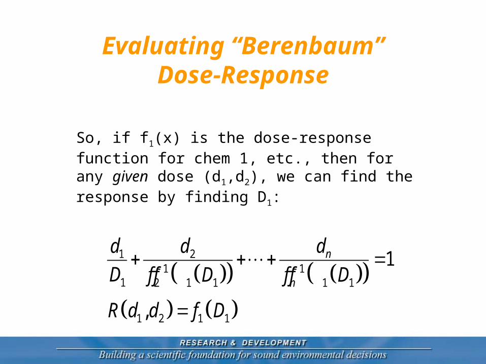
Evaluating “Berenbaum” Dose-Response

So, if f1(x) is the dose-response function for chem 1, etc., then for any given dose (d1,d2), we can find the response by finding D1:

1 21 1

1 2 1 1 1 1

1 2 1 1

1

,

n

n

dd d

D f f D f f D

R d d f D

DR for 50-50 Mixture

From PBPK

From RPFs

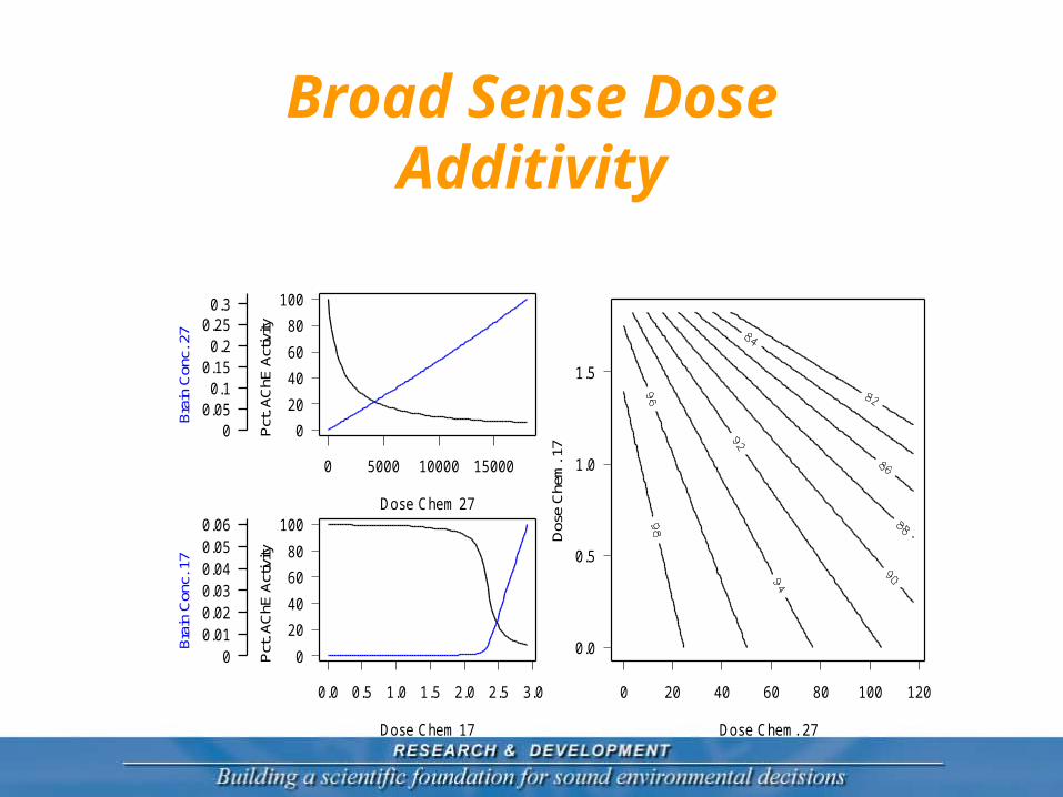
Broad Sense Dose Additivity

Dose Chem. 27

Dos

e C

hem

. 17

0 20 40 60 80 100 120

0.0

0.5

1.0

1.5

0 5000 10000 15000

0

20

40

60

80

100

Dose Chem 27

Pct

. AC

hE A

ctiv

ity

00.05

0.10.15

0.20.25

0.3

Bra

in C

onc.

27

0.0 0.5 1.0 1.5 2.0 2.5 3.0

0

20

40

60

80

100

Dose Chem 17

Pct

. AC

hE A

ctiv

ity

00.010.020.030.040.050.06

Bra

in C

onc.

17

DR for 50-50 Mixture

From PBPK

From RPFs

“Berenbaum”

Dose-Additivity “Dogma”

• What happens when two chemicals that are identical except for Ki are combined? (Same “mode of action”?) Chem 17: Ki = 11.04 Chem 300: Ki = 0.01, other parameters

the same

• Potency of 17 relative to 300 (ratios of BMD10) is ~ 4.25

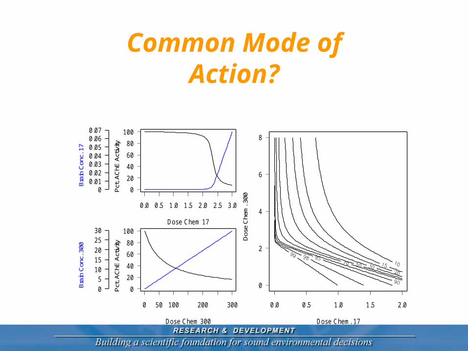
Common Mode of Action?

Dose Chem. 17

Dos

e C

hem

. 300

0.0 0.5 1.0 1.5 2.0

0

2

4

6

8

0.0 0.5 1.0 1.5 2.0 2.5 3.0

0

20

40

60

80

100

Dose Chem 17

Pct

. AC

hE A

ctiv

ity

00.010.020.030.040.050.060.07

Bra

in C

onc.

17

0 50 100 200 300

0

20

40

60

80

100

Dose Chem 300

Pct

. AC

hE A

ctiv

ity

05

1015202530

Bra

in C

onc.

300

Future Work

• OPCRA: Dose-response modeling is complete, tolerances being reassessed now.

• “Toy Models”: Explore other combinations Can we duplicate real OP dose-responses

without two sites on AChE? Activation Consequences for DR shape of metabolic

clearance in the blood.