domingo/teaching/ciic8996/Formal Analysis of... · Formal Analysis of Automated Model Abstractions...

Formal Analysis of Automated Model Abstractions underUncertainty: Applications in Systems Biology

A dissertation submitted to the

Division of Research and Advanced Studiesof the University of Cincinnati

in partial fulfillment of therequirements for the degree of

DOCTOR OF PHILOSOPHY

in the Department of Computer Scienceof the College of Engineering

July, 2011

by

Krishnendu Ghosh

M.S. (Mathematics), University of Wisconsin, Milwaukee, WIAugust 2001.

Dissertation Advisor and Committee Chair: John Schlipf, Ph.D.

All rights reserved

INFORMATION TO ALL USERSThe quality of this reproduction is dependent on the quality of the copy submitted.

In the unlikely event that the author did not send a complete manuscriptand there are missing pages, these will be noted. Also, if material had to be removed,

a note will indicate the deletion.

All rights reserved. This edition of the work is protected againstunauthorized copying under Title 17, United States Code.

ProQuest LLC.789 East Eisenhower Parkway

P.O. Box 1346Ann Arbor, MI 48106 - 1346

UMI 3503763

Copyright 2012 by ProQuest LLC.

UMI Number: 3503763

Abstract

In this dissertation, three fundamental problems in modeling of large scale biological systems

are addressed.

1. Modeling of chemical reactions under imprecise rate of reactions: A framework is cre-

ated to model chemical reactions with an interval based approach, incorporating im-

precision as well as creating a finite space. Algorithms are presented to construct

model abstraction efficiently. The results of the algorithms on a prototype elucidate

the model. The formalism presents a novel way to represent continuous data of con-

centrations for the chemicals and quantitative analysis of temporal behavior of the

system.

2. Multiscale formalism in discrete domains: Biological processes are multiscale. We

formalize the definition of multiscale modeling in discrete domains. A polynomial al-

gorithm is constructed to compute identifiability of multiscale systems.

3. Formal analysis of gene regulatory network: A formalism that incorporates noise in the

data is presented to study gene regulation. Computational efficiency of the formalism

is evaluated on a prototype constructed from biological experimental data.

Dedicated to Ma and Baba

Acknowledgements

PhD program has been a journey for me. I acknowledge all the people and their efforts

that made my journey, a memorable and rewarding one. My advisor, Dr. Schlipf, taught me

how to create science from disorganized ideas. My numerous meetings with him included

brainstorming of ideas and thinking out of box to seek an elegant solution. His exemplary

mentorship cannot be fathomed by words, rather it is imprinted and imbibed in my ability

to think precise formulation of problems. I, sincerely thank Dr. Schlipf for his contribution

in my development as a researcher.

I extend my gratitude and appreciation to my dissertation committee members- Dr.

Bhatnagar, Dr. Cheng, Dr. Medvedovic and Dr. Stan for their valuable suggestions and

guidance. I thank Dr. Bhatnagar for recruiting me as a graduate student and finding time

for me to answer my never ending set of questions. I thank Dr. Medvedovic for teaching me

how to become an effective communicator when interacting with biologists and statisticians.

Dr. Medvedovic supported my graduate assistantship for three years and had given me a

flexible schedule. I am grateful to him. I thank Dr. Cheng and Dr. Stan, for the pertinent

suggestions to enhance the quality of research. I thank the department of computer science

for supporting me with teaching assistantship for three years.

The PhD program would not be more enjoyable for me without the stimulating conver-

sations with Eric, Julia, Ryan and Tamisrada. In this journey, I thank the support of my

roomates, Vineet, Saurav, Susmit, Amlan, Ananda and Anubendu, who were patient to deal

with my idiosyncrasies and were always there to help me. I thank my friends, Angan, Sayan

and Shubhankar for making graduate life enjoyable. I thank Lisa, Shane and Ryan for always

finding time for me to put a smile on my face.

Words are not enough to thank my parents- Baba(father) and Ma(mother). My father

inspired me to pursue my dreams, instill discipline and resilience to fulfil my goals. My

mother always supported me in my life journey. She took away all the worries and hardships

so that her son could focus and pursue his dreams. I am inspired to write a better version of

Gorky’s ,The Mother. I thank my sister, Rinku for always being there for me and encouraging

me whenever I needed.

i

Table of Contents

1 Introduction 1

1.1 Formal Analysis in Systems Biology . . . . . . . . . . . . . . . . . . . . . . . 2

1.2 Automated Model Abstraction Under Uncertainty . . . . . . . . . . . . . . . 2

1.3 Contributions . . . . . . . . . . . . . . . . . . . . . . . . . . . . . . . . . . . 3

1.3.1 Temporal Reasoning for Chemical Reaction System . . . . . . . . . . 3

1.3.2 Multiscale Models in Discrete Domains . . . . . . . . . . . . . . . . . 3

1.3.3 Formal Analysis of Gene Regulation Network . . . . . . . . . . . . . 4

1.4 Outline of this dissertation . . . . . . . . . . . . . . . . . . . . . . . . . . . . 4

2 Background: Model Checking 6

2.1 System Modeling . . . . . . . . . . . . . . . . . . . . . . . . . . . . . . . . . 6

2.2 Model checking . . . . . . . . . . . . . . . . . . . . . . . . . . . . . . . . . . 7

2.2.1 LTL . . . . . . . . . . . . . . . . . . . . . . . . . . . . . . . . . . . . 8

2.2.2 CTL . . . . . . . . . . . . . . . . . . . . . . . . . . . . . . . . . . . . 9

2.2.3 Expressivity of CTL and LTL . . . . . . . . . . . . . . . . . . . . . . 11

2.3 Stochastic Models . . . . . . . . . . . . . . . . . . . . . . . . . . . . . . . . . 11

2.4 Probabilistic Model checking . . . . . . . . . . . . . . . . . . . . . . . . . . . 13

2.5 PCTL . . . . . . . . . . . . . . . . . . . . . . . . . . . . . . . . . . . . . . . 14

2.5.1 Syntax of PCTL: . . . . . . . . . . . . . . . . . . . . . . . . . . . . . 14

2.5.2 Semantics of PCTL . . . . . . . . . . . . . . . . . . . . . . . . . . . . 14

ii

2.5.3 Expressivity and complexity of PCTL . . . . . . . . . . . . . . . . . . 16

3 Prelimimaries: Chemistry, Biology and Model Construction 17

3.1 Reasoning from Chemical Kinetics . . . . . . . . . . . . . . . . . . . . . . . . 17

3.1.1 Physical Conditions affecting chemical kinetics . . . . . . . . . . . . . 17

3.1.2 Chemical Kinetics Theory . . . . . . . . . . . . . . . . . . . . . . . . 18

3.2 Genes and Gene Network . . . . . . . . . . . . . . . . . . . . . . . . . . . . . 19

3.3 Modeling of chemical reactions . . . . . . . . . . . . . . . . . . . . . . . . . . 20

4 Model Abstraction for Chemical Reactions 22

4.1 Formal methods in reasoning of biochemical pathways . . . . . . . . . . . . . 22

4.2 Preliminaries . . . . . . . . . . . . . . . . . . . . . . . . . . . . . . . . . . . 23

4.2.1 Rules for chemical reactions . . . . . . . . . . . . . . . . . . . . . . . 24

4.2.2 Definitions of Chemical Reaction . . . . . . . . . . . . . . . . . . . . 25

4.2.3 Model Assumptions . . . . . . . . . . . . . . . . . . . . . . . . . . . . 27

4.3 System Modeling . . . . . . . . . . . . . . . . . . . . . . . . . . . . . . . . . 29

4.3.1 Interval Representation of the concentration . . . . . . . . . . . . . . 32

4.4 Model . . . . . . . . . . . . . . . . . . . . . . . . . . . . . . . . . . . . . . . 32

4.4.1 The Kripke Transition Structure for a Set of Reactions . . . . . . . . 32

4.4.2 Features of the Chemical Reaction System . . . . . . . . . . . . . . . 35

4.4.3 Pruning . . . . . . . . . . . . . . . . . . . . . . . . . . . . . . . . . . 37

4.4.4 Rules of Pruning . . . . . . . . . . . . . . . . . . . . . . . . . . . . . 40

4.4.5 Properties of Kripke Transition System . . . . . . . . . . . . . . . . . 41

4.5 Initialization of the chemical reaction system . . . . . . . . . . . . . . . . . . 41

4.5.1 Modeling Equal Priority Reactions . . . . . . . . . . . . . . . . . . . 42

4.5.2 Approximating Chemical Reactions in the Kripke Transition System . 42

4.5.3 On-the-fly construction of Kripke transition system . . . . . . . . . . 43

iii

4.6 Construction of Kripke transition system for interval approximations . . . . 44

4.7 Discussion . . . . . . . . . . . . . . . . . . . . . . . . . . . . . . . . . . . . . 56

5 Formal Analysis of ERK Pathway 57

5.1 ERK Pathway . . . . . . . . . . . . . . . . . . . . . . . . . . . . . . . . . . . 57

5.2 Simulation of the ERK pathway . . . . . . . . . . . . . . . . . . . . . . . . . 59

5.2.1 Kripke transition system representing ERK pathway . . . . . . . . . 59

5.2.2 Results from simulation of ERK pathway . . . . . . . . . . . . . . . . 61

5.3 Guided Refinements in Computations . . . . . . . . . . . . . . . . . . . . . . 64

5.4 Discussion . . . . . . . . . . . . . . . . . . . . . . . . . . . . . . . . . . . . . 65

6 Multiscale System Design 66

6.1 Introduction . . . . . . . . . . . . . . . . . . . . . . . . . . . . . . . . . . . . 66

6.2 Background and Prior Work . . . . . . . . . . . . . . . . . . . . . . . . . . . 68

6.3 Formal Modeling of Multiscale Processes . . . . . . . . . . . . . . . . . . . . 71

6.4 Computation of Equivalences on LTS . . . . . . . . . . . . . . . . . . . . . . 73

6.5 Conclusion . . . . . . . . . . . . . . . . . . . . . . . . . . . . . . . . . . . . . 79

7 Formal Analysis of Gene Regulatory Relationships 80

7.1 Introduction . . . . . . . . . . . . . . . . . . . . . . . . . . . . . . . . . . . . 80

7.2 Preliminaries . . . . . . . . . . . . . . . . . . . . . . . . . . . . . . . . . . . 82

7.2.1 The Network model . . . . . . . . . . . . . . . . . . . . . . . . . . . . 82

7.2.2 The Control problem . . . . . . . . . . . . . . . . . . . . . . . . . . . 83

7.2.3 Chain functions . . . . . . . . . . . . . . . . . . . . . . . . . . . . . . 84

7.2.4 Regulatory Relationship Model . . . . . . . . . . . . . . . . . . . . . 86

7.3 Kripke structure representing regulatory relationship . . . . . . . . . . . . . 90

7.4 Application of the Regulatory-Relation to Galactose Utilization Pathway in

Yeast . . . . . . . . . . . . . . . . . . . . . . . . . . . . . . . . . . . . . . . . 91

iv

7.4.1 Galactose Utilization Pathway . . . . . . . . . . . . . . . . . . . . . . 92

7.4.2 Regulatory Relationship Model of the Galactose Pathway . . . . . . . 92

7.4.3 Noise in Gene Expression . . . . . . . . . . . . . . . . . . . . . . . . 94

7.4.4 Model Construction . . . . . . . . . . . . . . . . . . . . . . . . . . . . 95

7.4.5 Simulation . . . . . . . . . . . . . . . . . . . . . . . . . . . . . . . . . 96

7.4.6 Results from simulation of Galactose Pathway . . . . . . . . . . . . . 97

7.5 Discussion . . . . . . . . . . . . . . . . . . . . . . . . . . . . . . . . . . . . . 98

8 Future work 100

Bibliography 102

Appendix A. 116

v

List of Tables

4.1 Preprocessing on Kripke Transition System . . . . . . . . . . . . . . . . . . . 38

5.1 Time (in seconds) taken to read the files for interval midpoint approximation

and interval approximation. ”-” represents time greater than 15 minutes. . . 63

5.2 Execution times (in seconds) for CTL queries on ERK prototype using mid-

point approximation after the construction of model . Query 1-2,3-4, 5-6 and

7-8 represent reachability,pathway, checkpoint and stability properties on the

ERK prototype, repectively. . . . . . . . . . . . . . . . . . . . . . . . . . . . 63

5.3 Execution times (in seconds) for CTL queries on ERK prototype using interval

approximation after the construction of model on the identical set of queries

in Table 5.2. ”-” represents time greater than 15 minutes. . . . . . . . . . . 64

7.1 Execution times(in seconds) for PCTL queries on a regulatory relationship

construction using galactose dataset [Idekar et al.,2001] .”-” represents greater

than 20 minutes. . . . . . . . . . . . . . . . . . . . . . . . . . . . . . . . . . 98

8.1 Rate of Reactions [Cho et al.,2003, Calder et al.,2010] . . . . . . . . . . . . . 118

8.2 Initial Mass of the biochemicals in ERK pathway . . . . . . . . . . . . . . . 118

vi

List of Figures

2.1 A Kripke structure with initial state s0 . . . . . . . . . . . . . . . . . . . . . 8

3.1 Variation of enthalpy in a reaction(adapted from [Castellan,1983]) . . . . . . 19

3.2 Initiation of transcription . . . . . . . . . . . . . . . . . . . . . . . . . . . . . 20

4.1 Chemical properties controlling a chemical reaction . . . . . . . . . . . . . . 28

4.2 A Kripke transition system . . . . . . . . . . . . . . . . . . . . . . . . . . . . 31

5.1 RKIP inhibited ERK pathway (The same figure appeared in [Calder et al.,2006,

Shankland et al.,2005] . . . . . . . . . . . . . . . . . . . . . . . . . . . . . . 58

5.2 Kripke transition system representing ERK pathway with midpoint approxi-

mation . . . . . . . . . . . . . . . . . . . . . . . . . . . . . . . . . . . . . . . 61

6.1 Graphical structures showing similar ordering of reactions A,B and C repre-

sented by edge labels a,b and c, respectively . (A) Graph shows there are

consecutive processes. The label 10a in the dotted edge imply there are con-

secutive 10 edges labeled with a. (B) Graph shows there is no consecutive

labels on the edges. . . . . . . . . . . . . . . . . . . . . . . . . . . . . . . . . 67

7.1 Transcriptional regulatory network motifs [Blais et. al.,2005] . . . . . . . . . 88

7.2 Galactose Pathway (adapted from [Idekar et al.,2001]) . . . . . . . . . . . . . 93

7.3 Representation of regulatory relationship in stochastic formalisms. . . . . . . 97

vii

Chapter 1

Introduction

The advances in high throughput technologies and genome sequencing projects have pro-

vided impetus in the investigation of dynamics and interrelationships of biological entities as

integrated systems. The studies conducted in traditional molecular biology focused on bio-

logical entities such as genes, proteins and their functions individually and in isolation. The

protocols in molecular biology provided a myopic level of understanding of genes and gene

products. Kitano [Kitano,2002a] advocated systems-level understanding in systems biology

consisting of the biological entities and their interrelationships. A systems biology approach

includes identification of system structure comprising of network structures and interconnec-

tions of biological entities, investigation of system dynamics of the biological entities under

various conditions, control of the system entities with the aim to minimize noise and pro-

vide putative drug targets for diseases and finally, design and construction of the system

with the biological insights and simulation strategies substituting the ”trail-error” approach.

Complexity of living systems is a bottleneck for a detailed understanding and it is expensive

to perform biological experiments to collect data. Hence, there is need to construct com-

putational models to generate hypotheses to explain the experimental data and unravel the

interrelationships with system entities. Computational models are developed with emphasis

in understanding the intricate interrelationships and validation of the hypotheses from data

1

from biological experiments.

1.1 Formal Analysis in Systems Biology

Computational models in systems biology are created to automate the construction of the

relationships of gene and gene products from experimental data. The challenge in computa-

tional modeling is noise in the experimental data and imprecise parameters in the models.

The computational models are modeled on biological knowledge and hypotheses. Analysis of

biological experimental data is performed using the computational models. The results and

predictions generate hypotheses to be validated. The validation of hypotheses leads to refine-

ment of the biological knowledge, the basis for construction and revision of computational

models. The process is iterated with the aim of model validation on the biological experi-

mental data. Formal analysis, in particular model checking, seeks to prove the correctness

of the property in a given model, automatically. If the model does not fulfil the property

it returns, a counterexample is produced to debug and refine the model. The biological

properties are posed as queries, represented by temporal logic formulas to the model.

1.2 Automated Model Abstraction Under Uncertainty

Model abstraction in formal methods [Hsieh et al.,1998] is described as a process to reduce

the number of states for formal verification without losing behavioral properties of the orig-

inal model. The goal is to create a prototype that capture dynamics of relevant properties

of original model for verification of specifications on the model [Sinha et al.,2001]. Auto-

mated model abstraction algorithms reduce states by providing approximations in the model

abstraction. Large systems have inherent complexities in the form incomplete knowledge

of parameters of the system and integration of multiscale processes. Automated model ab-

straction is a key to analyze the temporal behavior of the system. The uncertainty in the

2

model parameters create challenges in the model analysis because of explosion of cases that

are to be considered for understanding accurate behavior of the model.

1.3 Contributions

1.3.1 Temporal Reasoning for Chemical Reaction System

The dissertation addresses a novel theoretical formalism for network inference. The for-

malism is able to answer quantitative (real) temporal logic queries and is comparable with

published models [Chabrier et al.,2003, Batt et al.,2005]. The formalism addresses imprecise

rate of chemical reactions and approximations to incorporate real values of concentrations of

biochemicals that are important in biological system modeling than boolean values. Two dif-

ferent algorithms are constructed to incorporate imprecision in the concentration, namely the

midpoint approximation and interval approximation. Deterministic and non-deterministic

models are constructed and evaluated on a prototype of ERK signalling pathway. The results

show one can evaluate, relatively efficiently, quantitative temporal queries on the models.

The novel formalism is able to provide a framework to reason using temporal logic without

the differential equations commonly used in hybrid system modeling. The approximations

used in the framework are able to represent uncertainty in the values of the chemical con-

stants.

1.3.2 Multiscale Models in Discrete Domains

Multiscale systems integrate entities that execute at different time scales. Large scale system

design combined with state explosion problem in model checking are constraints in biological

systems that necessitate multiscale approaches. Multiscale modeling in biology is critical in

understanding the connection between different levels of biological entities such as molecular,

3

cellular or atomic level. We formalize modeling of multiscale processes in discrete domains.

A polynomial time algorithm to compute equivalences between two multiscale models rep-

resenting identical processes is constructed. The formalism provide insights to solve the

identifiability of hidden markov models [Blackwell et al.,1957].

1.3.3 Formal Analysis of Gene Regulation Network

A novel formalism is created for an automated construction of gene networks directly from

gene expression data. The formalization allows us to reason about regulatory relationships

between genes taking into account intrinsic and extrinsic noise in the gene expression data.

The approach uses concepts in stochastic models such as markov model and markov decision

process. The formalism is evaluated for the computational efficiency in the construction of

the gene regulation network using probablistic temporal logic queries.

1.4 Outline of this dissertation

The structure of the dissertation is the following:

Chapter 2: contains concepts of model checking and temporal logics such as LTL and CTL.

The descriptions of stochastic models and probabilistic logic queries using PCTL are

stated.

Chapter 3: describes the definitions and concepts from chemistry and biology that are foun-

dational in modeling and analysis. The chapter contains concepts of modeling for-

malisms that are used later in this dissertaion.

Chapter 4: contains related work in chemical modeling , our contributions in formal modeling

chemical reaction network. The chapter describes the algorithms and approximations

for modeling uncertainty in the chemical reactions.

4

Chapter 5: details the implementation of the formal models described in chapter 4 on a

prototype representing the ERK pathway. Analysis on the computational model using

CTL and LTL queries are evaluated.

Chapter 6: states the contribution in the formalizations and definition of multiscale formal-

ism in discrete domains. A polynomial algorithm computes equivalences for multiscale

models.

Chapter 7: states the contributions in the automated construction of of gene network. Prob-

abilistic models incorporating noises have been described. A prototype of the model

is implemented on the galactose pathway to elucidate computational efficiency of the

model.

Chapter 8: contains the immediate and long term future research directions based on the

results of this dissertation.

Appendix A: contains the data for the simulation in the dissertation.

5

Chapter 2

Background: Model Checking

2.1 System Modeling

In this section, we explain system modeling to check the correctness of the system with a

given set of properties as reported [Clarke et al.,1986]. The first step for system verification

is the identification of the properties that is to be investigated on the system. The second

step is construction of a formal model capturing the properties that are to be considered

to verify its correctness. In this work, our focus is modeling a reactive system represent-

ing a system of chemical reactions and querying its dynamics over time. A reactive system

[Manna et al.,1991] maintains ongoing interaction(s) with its environment. The interac-

tions between the reactive system and its environment do not terminate [Clarke et al.,1986].

Hence, the system does not follow the input-output behavior. One of the important fea-

tures of a reactive system is a state. A state of the system gives a value of the variables

at a particular instant of time. The dynamics of system associated with the change in the

value(s) of the variable is captured by pair 〈s, s′〉 called a transition of the system. The com-

putations of a reactive systems defined in [Clarke et al.,1986] is an infinite system of states

where each state is obtained from the previous state by some transition. A state transition

graph, Kripke structure is an abstraction of the dynamics and behavior of a reactive system.

6

A Kripke structure consists of set of states, set of transitions and labeling function that

labels each state with the set of properties true in the state. Computations in a system is

represented by paths in the Kripke structure.

2.2 Model checking

In this section, we describe model checking and different temporal logics,such as linear tem-

poral logic(LTL) [Pneuli,1981] and computation tree logic(CTL) [Clarke et al.,1986].

Definition 2.1. (Model checking) Given a model,M and formula,φ , model checking is the

process of deciding whether a formula φ is true in the model, written M |= φ.

An appropriate knowledge representation structure such as Kripke structure,M = 〈S,R, Ls〉

given by:

Definition 2.2. A Kripke structure M over a set AP of proposition letters is a tuple

M = 〈S0, S, R, L〉 where,

1. S is a finite and nonempty set of states.

2. S0 ⊆ S is a set of states called the initial states.

3. R is a transition relation,R ⊆ S × S.

4. L : S → 2AP is the labeling function that labels s ∈ S with the atomic propositions

that are true in s.

A transition system is a Kripke structure 〈S0, S, R, L〉 where, for each state s ∈ S, there is

at least one state s′ ∈ S where (s, s′) ∈ R.

The intuition is:

1. There is only a finite set S of possible configurations of the system. At any time, the

system is in one of those configurations.

7

2. S0 is the set of states in which the system might be at time 0.

3. If the system is in state s at one time, when the state changes the system will move to

one of the states s′ where (s, s′) ∈ R.

4. L(s) is the set all atomic facts true when the state is in state s.

Figure 2.1: A Kripke structure with initial state s0

Here a transition system is constructed and physical information of the chemical reactions

or biological system is incorporated in a way to use the existing well studied logics such as,

LTL [Pneuli,1981] and CTL[Clarke et al.,1986]. We refer the reader to [Huth et al.,2003] for

an introduction.

2.2.1 LTL

We describe LTL [Pneuli,1981] model checking over M.

Syntax of LTL φ ::= > |⊥| p | (¬φ) | (φ ∧ φ) | (φ→ φ) | Xφ | Fφ | Gφ | φUφ

where p is any proposition. Operators X, F , G, and U are temporal operators : X means

next state,G for all states in future,F means in some state in future and U means until.

Semantics of LTL Start by defining satisfaction of formulas by infinite paths

π = s1, s2, s3, . . . in M. πi denotes the path starting with si, i.e, with nodes s1, . . . , si−1

removed.

1. π |= >.

8

2. π 6|=⊥.

3. π |= p if p ∈ L(s0).

4. π |= ¬φ if and only if π 6|= φ.

5. π |= φ1 ∧ φ2 if and only if π |= φ1 and π |= φ2 .

6. π |= φ1 ∨ φ2 if and only if π |= φ1 or π |= φ2.

7. π |= φ1 → φ2 if and only if π 6|= φ1 or π |= φ2.

8. π |= Xφ if and only if π2 |= φ.

9. π |= Gφ if and only if ∀i ≥ 1, πi |= φ.

10. π |= Fφ if and only if there is some i ≥ 1 such that πi |= φ.

11. π |= φUψ if and only if there is some i ≥ 1 such that πi |= ψ and ∀j = 1, . . . i− 1,

πj |= φ.

Finally, for any formula φ,M |= φ if every infinite path whose first state is in S0 satisfies φ.

2.2.2 CTL

We describe CTL [Clarke et al.,1983] model checking over M.

Syntax of CTL

φ ::= > | p | (¬φ) | (φ ∧ φ) | (φ→ φ) | Aψ | Eψ

ψ ::= φ | Xφ | φUφ | Fφ | Gφ

A and E are universal and existential quantifiers over paths out of the current state. The

syntax guarantees that each temporal operator is coupled with a preceding path quantifier.

Semantics of CTL Start by defining satisfaction of formulas at individual states of the

model:

1. M, s |= > and M, s 6|=⊥, ∀s ∈ S .

9

2. M, s |= p if p ∈ L(s).

3. M, s |= ¬φ if and only if M, s 6|= φ .

4. M, s |= φ1 ∧ φ2 if and only if M, s |= φ1 and M, s |= φ2

5. M, s |= φ1 ∨ φ2 if and only if M, s |= φ1 or Mn, s |= φ2

6. M, s |= φ1 → φ2 if and only if M, s 6|= φ1 or M, s |= φ2

7. M, s |= AXφ if and only if ∀s1 s→ s1 , M, s1 |= φ.

8. M, s |= EXφ if and only if ∃s1 s→ s1 M, s1 |= φ.

9. M, s |= AGφ if and only if for all paths s1 → s2 → s3 → . . . ,where s1 = s and for all

si along the path, M, si |= φ .

10. M, s |= EGφ if and only if there is a path s1 → s2 → s3 → . . . ,where s1 = s and for

all si along the path, implies M, si |= φ.

11. M, s |= AFφ if and only if for all paths s1 → s2 → s3 → . . . ,where s1 = s and there

is some si along the path, implies M, si |= φ.

12. M, s |= EFφ if and only if there is a path s1 → s2 → s3 → . . . ,where s1 = s and

there is some si along the path, implies M, si |= φ.

13. M, s |= A[φ1Uφ2] holds if and only if for all parths s1 → s2 → s3 → . . . where s1 = s.

that path satisfies φ1Uφ2 such that M, si |= φ2 and for each j < i ,Mnsj |= φ1.

14. M, s |= E[φ1Uφ2] holds if and only if there is a path s1 → s2 → s3 → where s1 equals

s and that path satisfies φ1Uφ2. M |= φ” means that every start state of M satisfies

φ.

Theorem 2.1. (Time complexity of CTL model checking [Clarke et al.,1986]) The time

complexity of the modelchecking problem of a given CTL in a model, M = 〈S,R, L〉 is

O(length(φ)(| S | + | R |).

Theorem 2.2. (Time complexity of LTL model checking [Sistla et al.,1985]) The time

complesity of the model checking problem of a given LTL in a model, is PSPACE complete.

10

2.2.3 Expressivity of CTL and LTL

We complete the discussion of CTL and LTL with comparing expressiveness of the

temporal logics,CTL and LTL. There are some queries that can be expressed in LTL but

not in CTL and vice versa. A LTL formula such as FGφ cannot be expressed in CTL.

Conversely, there are CTL formulas that are not expressed because of the limited

expressive power of LTL. In the case CTL, there is a path quantifier A or E before the

operators X,F and G. On the other hand, LTL does not have existential quantifier on its

path and hence, only “for all paths” that is A can be expressed. A CTL formula,AG(AFφ)

cannot be expressed in LTL. Also, there are forumlas, which cannot be expressed in either

LTL or CTL. An example of such an formula is A(FGφ) ∨ AG(AFφ). Hence, neither LTL

or CTL is an subset of each other.

2.3 Stochastic Models

In this section, definition of stochastic models are stated. There are two classes of

stochastic model based on the discrete and continous spaces. The discrete markov models

are discrete-time chain and markov decision process. Continuous-time markov chain is

stochastic model that describes time as a continuous parameter. In this dissertation, the

modeling of gene-regulation relationships is limited to discrete markov models. (For a

description of continuous models, see [Hermanns,2002].)

Definition 2.3. (Discrete-Time Markov Chains) A simple model of Markov chains is

discrete-time Markov chains (DTMC) is described formally, K〈S, S0, P, L〉 where

• S is a finite set of states.

• S0 is the initial state.

• P : S × S → [0, 1] , where P represents the probability matrix and∑

s,s′∈SP (s, s′) = 1.

11

• L : S → 2AP . AP is the set of atomic propositions.

The following description in paraphrased from [Parker,2002]: Terminating states can be

modeled with a self loop with probability one. A path, π through a DTMC is a sequence of

states s0s1s2, . . . is a sequence of non-empty states with a probability,P (s, s′) > 0∀i ≥ 0 .

We describe the definitions of probability measure on path. The notation is the following:

For any path π, the i state is denoted by π(i). A finite path of length m is usually denoted

πm. The set of infinite paths starting from s is given by Path(s).

The definition of probability measure, Prs on Path(s) is given in

[Parker,2002, Kemeny et al.,1966]. First define probabilities for finite paths πm. The

probability of any path of length 1 is 1. For a path πm = s0, s1, . . . , sm,

P (πm) = P (s0, s1) · P (s1, s2) · · ·P (sm−1, sm). Second, define probabilities for sets of infinite

paths: Let C(πm) be the set of all paths with prefix πm, and define probability

Prs(C(πm)) = P (πm). Extend probabilities to other sets as usual in probability theory.

Definition 2.4. (Markov Decision Processes) A generic model of DTMC is a Markov

Decision Processes (MDP). MDP models nondeterministic and probabilistic systems with

processes executing in parallel. Formally, a MDP is Km〈S0, S,A,P ,L〉 [Puterman,1994]

where

• S is a finite set of states.

• S0 is the initial state.

• A is the finite set of actions. 1

• P : S × A× S → [0, 1] and ∀a ∈ A, ∀s ∈ S∑s′∈S

P (s, a, s′) = 1

• L : S → 2AP . L represents the labeling function and AP represents is the set of

atomic propositions.

1A can be a set of subsets.

12

Clearly, the definition of markov chains show that they are proper subset of Markov

Decision Processes. In the discussion of probability measures, we summarize from

[Parker,2002]. Let H be a function that maps each state s ∈ S to finite,nonempty subset of

Dist(S) where Dist(S) is the set of all probability distributions ver S. Each µ ∈ Dist(S) is

of the form µ : S → [0, 1] where∑s∈S

µ(s) = 1. A path in a MDP is of the form

s0µ1→ s1

µ2→ s2 . . . where si ∈ S, µi+1 ∈ H(si) and µi+1(si+1) > 0 for all i ≥ 0. A path in a

MDP takes into account the nondeterminism and the probability. Assume the

nonderterministic choices are represented by the action. Using the notation from DTMC,

Path(s) is the set of all infinite paths from s. A finite path in a MDP is given by πm where

m ∈ N. Let A is a function defined on finite paths onto a probability distribution.

Formally, A(πm) ∈ H(sm). The notation, of a path for A is given by PathA(s) and

PathA(s) ⊆ Path(s). The details of probability measure PrA(s) on a set of paths,

PathA(s) is reported [Baier et al.,2002].

2.4 Probabilistic Model checking

Interpreting temporal logics over stochastic models such as discrete time markov chains

and markov decision models is probabilistic model checking.

Definition 2.5. (Probabilistic Model checking) Given a probabilistic model,Mp and

formula,φ ,model checking is the process of computing the answer to the question of

whether Mp |= φ holds.

It is important to note that in conventional model checkers give ”yes/no” answer.

Probabilistic model checking gives, instead, answers that are probabilities. We describe

probabilistic computation tree logic (PCTL) [Aziz et al.,1995, Hansson et al.,1994], an

extension of CTL on DTMCs and MDP.

13

2.5 PCTL

We describe the syntax of PCTL and semantics of PCTL over DTMCs and MDP. The

following is summarization from the published dissertation [Parker,2002].

2.5.1 Syntax of PCTL:

The syntax of PCTL is:

φ ::= true | p | φ ∧ φ | ¬φ | P⊕J [ψ]

ψ ::= Xφ | φU≤kφ | φUφ

where p is an atomic proposition,⊕ ∈ {≤, <,≥, >},J ∈ [0, 1] and k ∈ N. φ, ψ are state and

path formula respectively. φ and ψ are state and path formulas repectively. Each of these

formulas are interpreted over a DTMC or an MDP. Each state of DTMC or MDP is

labeled from the set of atomic proposition. Specification is represented in the form of a

state formula. Path formula ψ are preceded by the probability path operator P . Examples

of intervals that are bounds for P are : P≤0.5(ψ) denotes P[0,0.5](ψ). The meaning of a state

s of DTMC or MDP satisfies P⊕J is the probability of a path from s satisfying ψ is in the

bound stated by ⊕p. The path forumla, Xφ is true if φ is satisfied in the next state. The

formula φ1U≤kφ2 is true if φ2 is satisfied within k time-steps and φ1 is true till that point.

Similar is the description of φ1Uφ2 where φ2 is true some point in future and till then φ1 is

true.

2.5.2 Semantics of PCTL

In this section, we describe the semantics of PCTL on the stochastic models, DTMC and

MDP.

14

Semantics of PCTL over DTMC:: Given a DTMC, Mp = 〈S0, S,P , L〉 and a PCTL

formula, the notation s |= φ denotes that φ is satisfied in s. For a given path, π satisfying a

PCTL path formula, the notation is π |= ψ. The semantics of PCTL over Mp is

paraphrased from [Parker,2002]:

For a path π :

1. π |= Xφ if and only if π2 |= φ.

2. π |= φ1U≤kφ2 if and only if, for some ≤ k, πj |= φ2 and, for all j < i, πi |= φ1.

3. π |= φ1Uφ2 if and only if ∃k ≥ 0, π |= φ1U≤kφ2.

For a state, s ∈ S:

1. s |= true, ∀s ∈ S.

2. s |= a if and only if a ∈ L(s).

3. s |= φ1 ∧ φ2 if and only if s |= φ1 ∧ s |= φ2.

4. s |= ¬φ if and only if s 6|= φ.

5. s |= P⊕J [ψ] if and only if ps(ψ)⊕ p.

where ps(ψ) = Prs({π ∈ Path(s) | π ||= ψ}) where Prs is defined in Section 2.3.

Semantics of PCTL over MDP: The following discussion, we paraphrase from

[Parker,2002]. The semantics of PCTL over MDP are the identical with the semantics of

PCTL over DTMC. The computations of the probability of a set of paths in a MDP is for

an adversary. Notation: pAs (ψ) = PrAs ({π ∈ PathAs | π |= ψ}) where pAs (ψ) is the

probability that a path from s satisfies ψ under schedular (adversary) ,A. The semantics of

PCTL over MDP is in terms of quantification over a class of schedulars,Sdl.

1. s |=Sdl true ∀s ∈ S.

15

2. s |=Sdl a if and only if a ∈ L(s).

3. s |=Sdl φ1 ∧ φ2 if and only if s |=Sdl φ1 ∧ s |=Sdl φ2

4. s |=Sdl P⊕J if and only if pAs (ψ)⊕ p for all A ∈ Sdl.

The path formula can be expressed using ♦ operator: ♦φ is trueUφ, meaning that φ is

eventually true. The analogous bounded version of the specification ♦≤kφ means that φ is

satisfied within k time steps. The quantifiers on the set, Sdl, existentional and universal,

are also used in writing the specification.

2.5.3 Expressivity and complexity of PCTL

One of the limitations of PCTL is its expressibility. Some of the properties such as

♦φ1 ∧ ♦φ2 [Parker,2002] cannot be expressed. The formula, ♦φ1 ∧ ♦φ2 means that φ1 and

φ2 are eventually satisfied but not necessarily at the same time. The satifiability of the

formulas, ♦φ1 and ♦φ2 cannot be used for derivation of satisfiability of ♦φ1 ∧ ♦φ2. For

details on PCTL , refer the published literature

[Parker,2002, Kwiatkoska,2003, Aziz et al.,1995, Baier et al.,2002].

Theorem 2.3. (Time Complexity of PCTL model checking for DTMC

[Courcoubetis et al.,1988]) The time complexity for a given finite DTMC and PCTL

formula, φ, the model checking problem Mp |= φ can be solved in polynomial time in the

size of model Mp and linear in the size of the formula.

Theorem 2.4. (Time Complexity of PCTL model checking for MDP

[Courcoubetis et al.,1990]) The time complexity for a given finite MDP and PCTL formula,

φ, the model checking problem Mp |= φ can be solved in polynomial time in the size of

model Mp and linear in the size of the formula.

16

Chapter 3

Prelimimaries: Chemistry, Biology

and Model Construction

In this chapter, we describe the background definitions, methods and formalisms that form

the foundations of the dissertation.

3.1 Reasoning from Chemical Kinetics

Chemical reactions are governed by chemical kinetics and the chemical properties. Our

model incorporates chemical properties that have foundations un chemical kinetics theory.

3.1.1 Physical Conditions affecting chemical kinetics

We describe chemical kinetics and the theoretical background of chemical reactions from

the literature [Castellan,1983, Levine,2002]. The rate of reaction is defined by chemical

kinetics. Precisely, rate of reaction is the rate of increase of the advancement of reaction for

a substrate/product with time. The rate of reaction is a function of temperature, pressure

and the concentration of the various species in the reaction. It may also depend on the

concentration of the catalyst/inhibitors that may not appear in the overall rate equation of

17

the reaction. The rate of reaction may be proportional to the different powers of the

concentration of the substrates. The rate of reaction increase is given by the Arrhenius

equation: k = Ae−E/RT where k is the rate constant, A is called the frequency factor, E is

the activation energy. R is the universal gas constant and T is the temperature in Kelvin.

Chemical reactions are classified as homogeneous and heterogeneous reactions. A

homogeneous reaction occurs entirely in one phase, a heterogeneous reaction has atleast a

part of the reaction in more than one phase.

The rate of chemical reactions is directly proportional to the concentrations of the

reactants. The rate of reactions in liquid is the same as those in gas phase. Thus, the

chemical reactions can be studied in either liquid/gas phase because the mechanism is the

same. The rate of reaction is faster in liquid simply because of the increased concentration

of the reactants. The ionic reactions between the ions in solution occur very rapidly and

are stabilized by hydration.

3.1.2 Chemical Kinetics Theory

The rate constant for the forward reaction depends on the chemical properties of substrates

and the reverse rate depends on the chemical properties of the products. Enthalpy of a

system (comprising of chemicals), is the measure of total energy of the system. Figure 3.1

shows the variation of enthalpies of the substrates and products during a chemical reaction

with the qualitative notion of time.

HA, HP and HS are the total enthalpies of the activation, products and substrates

respectively. The quantity HA −HS, represents the energy quantity, E in the Arrhenius

equation, the energy that separates the reactant state from the product state. The

substrates must overcome the energy barrier for the formation of the products. The

magnitude of the energy barrier is given by HA −HS is the activation energy of the

forward direction, Ef . The magnitude of the activation energy in the reverse direction, Er

18

Figure 3.1: Variation of enthalpy in a reaction(adapted from [Castellan,1983])

is given by HA −HP . Hence, the relation Ef and Er is given by Er = Ef− (HS −HP ). A

chemical reaction is an endothermic reaction if HS −HP is negative and is exothermic if

positive. Therefore, the quantity of energy represented by HS −HP , determines if the

reaction is endothermic or exothermic.

3.2 Genes and Gene Network

In this section, we provide an outline of gene regulation by describing the functioning of

the basic elements to initiate regulation. The processs of protein and RNA production

from a gene is perfomed in two step procedure. In the first step, transcription, the

nucleotides, adenine(A),guanine(G), cytosine (C) and thymine (T) are replicated to

produce a single stranded messenger mRNA. Transcription is initiated by an enzyme,

RNA polymerase that binds to the promoter region of the gene as shown in Figure 4.1.

RNA binds-unbinds to the double stranded DNA with the consequence that the DNA

unwinds, generating a complementary strand of RNA. In the second step, translation, the

mRNA reacts with ribosome to produce amino acids. The production of gene products,

RNA and proteins from DNA is known as gene expression.

Advances in technology led to the completion of the Human Genome Project. The results

of the project were able to identify around 25000 genes in the human genome

19

Figure 3.2: Initiation of transcription

[Lander et al.,2001, Baltimore,2001]. The gene expression of a cell in human hair and in

human brain differ in the expression in the subset of the 25000 genes in each of the cases.

The diversity and complexity in the functionality of the cells is attributed to the gene

expression. Transcription is initiated and controlled by transcription factors (TF) that are

proteins. The TFs that prevents expression of are called repressors and the ones that

enhances expression are activators. In a gene, there are a number of transcription factors

binding sites (TFBS) for TF to bind because there are number of TFs that bind in the

promoter region. We refer the reader to [Cooper et al,2009] for details.

3.3 Modeling of chemical reactions

In this section, we review some of the challenges in model construction to model

biochemical processes as described [Thorsley et al.,2010]. Modeling of complex systems in

chemistry is intractable very complex. and hence, computationally intensive. Model

reduction is a process to reduce the model size and to study properties of a large scale

system under approximations. Modeling becomes tedius with the task of parameter

estimation for the chemical rate of reactions. The data for the rate of reactions is collected

from experiments. There is always a possibility that the reaction rate of certain chemical

reaction is not validated with experimental data. Parameters are estimated to bridge the

gap between the incomplete knowledge of the reaction and representation of the reaction in

20

the model. Modeling chemical reactions is important to unravel the underlying behavior of

the chemicals taking part in the reactions. The process of verifying the model behavior

equivalence [Thorsley et al.,2010] is model comparision. Quantification of the model

behavior is perfomed by model invalidation. In this dissertation, we describe a mechanistic

model for chemical reaction and a data dependent model for gene network construction. A

mechanistic model for chemical reactions [Gillespie,D.,1977] is based on the chemical

kinetics and the rate of reactions. The behavior of the model is solely studied from the

chemical parameters such as rate of reactions. The models that use biological experimental

data such as gene expression data to construct the biological processes for analysis are

known as data dependent models.

21

Chapter 4

Model Abstraction for Chemical

Reactions

4.1 Formal methods in reasoning of biochemical

pathways

We discuss the work in using formal methods in reasoning of biochemical pathways and

motivate the need for a new initiative to address quantitative reasoning on models of

biochemical pathways constructed with imprecision of data. Prior work incorporating

numerics in model checking has been published. Model checking by quantifying time

[Emerson et al.,1992] on real time systems and numerics in the form of weights have been

been discussed [Chatterjee et al.,2003].

A formalism for querying biomolecular interactions by representing and analyzing

protein-protein and protein-DNA interactions has been formulated

[Rivier-Chabrier et al.,2004] by creating a language and querying by temporal logic. A

complicated model by Batt et al.[Batt et al.,2005] was able to express quantitative queries

by incorporating the numeric quanitities of the gene and computing the derivatives of the

22

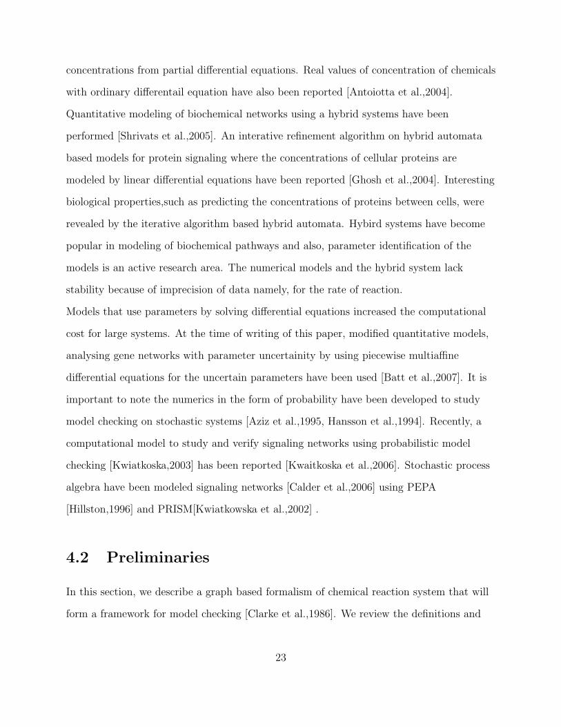
concentrations from partial differential equations. Real values of concentration of chemicals

with ordinary differentail equation have also been reported [Antoiotta et al.,2004].

Quantitative modeling of biochemical networks using a hybrid systems have been

performed [Shrivats et al.,2005]. An interative refinement algorithm on hybrid automata

based models for protein signaling where the concentrations of cellular proteins are

modeled by linear differential equations have been reported [Ghosh et al.,2004]. Interesting

biological properties,such as predicting the concentrations of proteins between cells, were

revealed by the iterative algorithm based hybrid automata. Hybird systems have become

popular in modeling of biochemical pathways and also, parameter identification of the

models is an active research area. The numerical models and the hybrid system lack

stability because of imprecision of data namely, for the rate of reaction.

Models that use parameters by solving differential equations increased the computational

cost for large systems. At the time of writing of this paper, modified quantitative models,

analysing gene networks with parameter uncertainity by using piecewise multiaffine

differential equations for the uncertain parameters have been used [Batt et al.,2007]. It is

important to note the numerics in the form of probability have been developed to study

model checking on stochastic systems [Aziz et al.,1995, Hansson et al.,1994]. Recently, a

computational model to study and verify signaling networks using probabilistic model

checking [Kwiatkoska,2003] has been reported [Kwaitkoska et al.,2006]. Stochastic process

algebra have been modeled signaling networks [Calder et al.,2006] using PEPA

[Hillston,1996] and PRISM[Kwiatkowska et al.,2002] .

4.2 Preliminaries

In this section, we describe a graph based formalism of chemical reaction system that will

form a framework for model checking [Clarke et al.,1986]. We review the definitions and

23

rules that form the basis of our quantitative model for representing a system of chemical

reactions.

4.2.1 Rules for chemical reactions

The chemical graph community have classified the chemical reactions in four classes based

on the atomic structure of the substrate and products [Rosello et al.,2004a]. The five rules

of chemical reactions are summarized in [Rosello et al.,2004a] for a given set of chemicals,C

= {A,B,C,AB,CD,AD,CB}. Also, AB,CD,AD and CB are formed by pairs of chemicals

(A,B),(C,D),(A,D) and (C,B),respectively.

Rule 1: The formation of single product from two or more substrates is given by the rule:

A + B → AB, where A,B are substrates and AB product respectively.

Rule 2: The formation of a two or more products formed by decomposition of a substrate

is of the form: A → B + C.

Rule 3: The products are formed by arrangement of the atoms of the substrate. A + BC

→ AC + B.

Rule 4: The products are formed by the exchange of the atoms of both the substrate,AB

+ CD → AD + CB.

Rule 5: A catalytic reaction is given by, A + CB → A + C+ B. In this reaction,A is the

catalyst. The catalyst(s) for the reactions gpverned by rules 1-4 can be represented

by chemical(s) appearing both as a substrate and product.

One of the important aspects of chemical reactions is the rate of reactions with respect to

amount of concentrations of the substrates. The chemical kinetics of the reactions is

governed by the laws of mass action and principle of equilibrium of chemical reaction

[Temkin et al.,1996] with respect to the concentrations of the chemicals in the reactions,

namely, substrates and products. Chemical reactions have been modeled using graphs and

24

hence, called chemical graphs [Temkin et al.,1996, Rosello et al.,2004a]. Modeling of

chemical reactions using chemical graphs in the form chemical reaction networks have been

described [Temkin et al.,1996, Benko et al.,1999]. Analysis of metabolic pathways have

been performed using directed graphs where the substrates, products, and enzymes were

represented by nodes and the chemical reactions by the edges of the graph

[Rosello et al.,2004].

4.2.2 Definitions of Chemical Reaction

A chemical reaction is represented by a formula

mAA+mBB + · · ·+mZZ → nAA+ nBB + · · ·+ nZZ

where the mX ’s and nY ’s are positive integers and the X’s and Y ’s are chemicals with

X ∈ {A, B, . . . , Z} and Y ∈ {A, B, . . . , Z} . The reading is that mA moles of chemical A,

mB moles of chemical B, . . .mZ moles of chemical Z react together to form nA moles of

chemical A, nB moles of chemical B, . . . and nZ moles of Z. A, . . . , Z are called substrates

of the reaction, and A, . . . , Z,products. Here, X, Y represents a single chemical or a set of

chemicals.

Definition 4.1. (Concentration) The amount of chemical A present in the system, called

the concentration of A, is represented by a.

Definition 4.2. (Reaction ratio of chemicals (substrates/products)) The reaction ratio of

a chemical (substrate/product) is the ratio of number of moles of the chemical

(substrate/product) to that of total number of moles (forming the substrates/products) in

the reaction. It is represented as ~XRatio = { ˆxrat1, . . . , ˆxratn} where X = S/P for set of

substrates/products, x = s/p represents each substrate/product and n ∈ N.

25

Example 4.1. (Reaction ratio) Given a reaction A + 6B → C + 3D. The total weight of

the substrates and products are 6 + 1 = 7 moles and 1 + 3 = 4 moles respectively. The

reaction ratio of substrates, A and B are given by 17

and 67

respectively. Similarly, the

reaction ratio of products are given by, C and D are, 14

and 34

respectively.

In the case of Rule 1 and Rule 2 of reaction, the reaction ratio of the single

product/substrate is equal to one. Below, let R+ denote the set of non-negative real

numbers.

Definition 4.3. A reaction tuple is a tuple given by

rtup = 〈 ~SRatio, ~PRatio,ForRate,RType,RevRate, ~Catalyst, ~Inhibitor〉

where

• ~SRatio = 〈 ˆsrat1, . . . , ˆsrati〉 where ˆsrati ∈ R+ represents the reaction ratio of i

substrates taking part in a reaction and i ∈ N.

• ~PRatio = 〈 ˆprat1, . . . , ˆpratj〉 where ˆpratj ∈ R+ represents reaction ratio of the j

products formed in a reaction and j ∈ N.

• ForRate ∈ R+ represents the rate of the reaction in the foward (→) direction,

• RevRate ∈ R+ represents the rate of the reaction in the backward (←) direction

• RType ∈ {−1, 0, 1} denotes the “type”of the reaction, where “-1”,“0” and “1”

represent endothermic, energy free and exothermic reaction,respectively. The priority

of reactions on RType is given by exothermic>energy free>endothermic.

• ~Catalyst = 〈 ˆcat1, . . . , ˆcatk〉 where ˆcatk ∈ R+ is the minimum amount for the chemical

to be neccessary to catalyze the reaction and k ∈ N. In the absence of a catalyst,

~Catalyst = 0

26

• ~Inhibitor = { înh1, . . . , înhk} where înhk ∈ R+ is the minimum amount chemical to

inhibit the reaction. In the absence of an inhibitor, ~Inhibitor = 0.

As a special case of a reaction tuple, we use ε = 〈~0,~0, 0, 0, 0, ∅, ∅〉 to represent there being

no reaction.

Definition 4.4. (Admissible reaction) A reaction is admissible if the following constraints

are fulfilled,

1. (Concentration of Substrates) The concentration of the substates should be atleast

the minimum concentration required to initiate the reaction.

2. (Concentration of Catalyst) If the reaction requires catalyst(s), the concentration of

the catalyst(s) should be atleast the minimum concentration(s) required to initiate

the reaction.

Definition 4.5. (Limiting chemical) A substrate(s) of a chemical reaction that is fully

consumed in the chemical reaction is a limiting chemical ,i.e, if the concentration of a

substrate z before the reaction is x moles, the concentration of z after the completion of

the reaction should be 0,then z is a limiting chemical.

4.2.3 Model Assumptions

The assumptions in our model:

1. We assume that the reactions are taking place in solution.

2. The external physical conditions such as temperature, pressure are assumed to be

constant during the reactions.(The external temperature does not influence the

system temperature.)

3. The forward rate of reaction is considered in our model. We can incorporate a reverse

rate by also including the reverse reaction with that rate.

27

4. All the reactions are assumed to be homogeneous, i.e., taking place in a single phase

(solution). This assumption would help us to have a single rate of reaction for a

particular reaction.

5. The reactions proceed till the concentrations of limiting substrates fall below the

minima required for the reaction.

Example 4.2. Given a reaction: 3A + B → 2C; if 3 moles of A reacts with 1 mole

of B then 2 moles of C is produced. If there are 7 moles of A and 1 moles of B

present in the chemical reaction system, then reaction will take place as long as the

molar ratio of A and B is maintained. In this case, only 3 moles of A will be used.

6. The reactions are controlled by chemical properties such as ionization potential,

solvation energy and lattice energy (Born-Haber Cycle). For example, for the given

reaction: Na(s) + 12X2 → NaX(aq), where X is any halogen,and s, g, aq represent

solid, gas and aqueous respectively, the chemical properties and chemical processes

(Born-Haber cycle) [Huheey et al.,1997] that control the reaction are shown in Figure

4.1 .

Figure 4.1: Chemical properties controlling a chemical reaction

Initially sodium,Na(s) in solid state changes into sodium vapors Na(g). The Na(g)

ionizes to sodium ions Na+ and halogen, X forms halogen ions,X− by gaining an

electron (electron affinity). There is a reaction between Na+ and X−. The energy

28

required to form NaX(s) is provided by lattice energy. Finally, NaX is formed in an

aqueous solution by giving off hydration energy.

7. The exothermic reactions are given higher precedence over endothermic reactions and

reactions, where no energy is liberated/required because exothermic reaction are

spontenous, evolving energy.

8. A catalyst is a substance that increases the rate of reaction and can be recovered

unchanged at the end of the reaction. If a substance slows a reaction, it is called an

inhibitor. The reactions that do not require catalyst are at a higher precedence than

a reaction that requires a catalyst. For the catalyst-initiated reaction to proceed

there has to be specific amounts of the catalyst in the solution. If the catalyst is not

present in the solution the “catalyst-reaction” will be slow (or the reaction cannot be

initiated at all). On the contrary, if a reaction requires an inhibitor, the reaction

would be at a higher precedence, because in the absence of inhibitor it will be more

vigorous.

9. The reactions take place when the substrate reach a threshold for a reaction. The

labels contain the information about the threshold levels of the substrates in a

reaction.

4.3 System Modeling

In this section, we explain system modeling to check the correctness of the system with a

given set of properties as reported in Clarke et al. [Clarke et al.,1986] .The first step for

system verification is the identification of the properties that are to be investigated on the

system. The second step is construction of a formal model capturing the properties that

are to be considered verification of its correctness. In this work, our focus is modeling a

reactive system representing a system of chemical reactions and querying its dynamics over

29

time. A reactive system [Manna et al.,1991] maintains ongoing interaction(s) with its

environment. The interactions between the reactive system and its enviroment does not

terminate [Clarke et al.,1986]. Hence, the system does not follow the input-output

behavior. One of the important features of a reactive system is a state. A state of the

systems gives a value of the variables at a particular instant of time. The dynamics of

system associated with the change in the value(s) of the variable is captured by pair 〈s, s′〉

called a transition of the system. A computation of a reactive systems defined in

[Clarke et al.,1986] is an infinite system of states where each state is obtained from the

previous state by some transition. A Kripke structure — a state transition graph — is an

abstraction of the dynamics and behavior of a reactive systems. A Kripke transition

system consists of set of states, set of transitions and labeling function that labels each

state with the set of properties true in the state. Computations in a system are represented

by paths in the Kripke transition system. Although we shall be working with Kripke

transition system, as part of our construction we shall use edge-labeled Kripke transition

system, which we call “E-Kripke transition system.”

Definition 4.6. A Kripke transition system M over a set AP of proposition letters is a

tuple M = 〈S0, S, R, L〉 where,

1. S is a finite and non empty set of states.

2. S0 ⊆ S is the set of initial states.

3. R is a transition relation,R ⊆ S × S such that for each s ∈ S there is at least one

s′ ∈ S and (s, s′) ∈ R

4. L : S → 2AP is the labeling function that labels s ∈ S with the atomic propositions

that are true in s.

Figure 4.2 represents a Kripke transition system . In the figure, p, q, r are the atomic

propositions s0, s1, s2 and s3 form the set of states,S for the Kripke transition system. The

transitions represent the relations between the states.

30

Figure 4.2: A Kripke transition system

Definition 4.7. (Edge-labeled)E-Kripke transition system) An edge labeled Kripke

transition system M over a set AP of proposition letters and a set E of labels is a tuple

M = 〈S0, S, R, Ls, Le〉 where,

1. 〈S0, S, R, Ls〉 is a Kripke transition system

2. Le : R→ E .

In this paper, AP will consist of formulas c = 0 or c ∈ (ci, ci+1] where c is the concentration

of one of the chemicals (substrates or products) being studied and (ci, ci+1] is one of the

concentration intervals for that chemical. A state will thus correspond to the (approximate)

concentrations of all the chemicals of interest. A transition (s, s′) where L(s) 6= L(s′) will

correspond to the change of state due to a chemical reaction’s taking place. A special case

of transition where a transition of the form (s, s) will be allowed to represent equilibrium,

i.e no reaction can take place further. Also,E will be the set of reaction tuples. In a state

where many reactions are possible, the priority on the reaction tuples will let us select

which reaction will take place first. The reduct Kripke transition system of an E-Kripke

transition system Me = 〈S0, S, R, Ls, Lr〉 is the Kripke transition system Mre〈S0, S, R, Ls〉.

31

4.3.1 Interval Representation of the concentration

The concentrations of the substrates and products in a reaction is represented by intervals.

Imprecise parameters in the reactions,namely the rate of reaction have been addressed by

making approximations [Batt et al.,2007] and by simulations [Cho et al.,2003]. In our

model, we address the imprecision in parameters by representing the concentration of the

chemicals in the form of intervals. Interval representation preserves the finiteness on

computation model and is an approximation to real computation. Prior work using interval

representation had been reported [Kifer et al.,1992].

4.4 Model

In this section, we describe the Kripke transition system for the set of chemical reactions

and then the important features of the Kripke transition system. A novel method pruning

is explained in details showing the model retains it accuracy with minimal simplications.

4.4.1 The Kripke Transition Structure for a Set of Reactions

We are given (1) a set C of chemicals, (2) for each chemical A ∈ C a set of intervals

{0}, (0, a1], (a1, a2], . . . (an,∞) in which to cluster the concentration of A, (3) a set of

chemical reactions,Rtuple with each reaction represented by its reaction tuple,rtup and

(4)for each reaction,rtup, 〈t, t′〉, where t and t′ represents the temperature before and after

the reaction. Additionally, we are also given a reaction tuple,ε with a pair of temperature

〈t, t〉 representing there is no change in temperature during no reaction. The E-Kripke

transition system Me = 〈S0, S, R, Ls, Lr〉 is as follows:

• AP is the set of all the atomic formulas a = 0, a ∈ (0, a1], or a ∈ (ai, ai+1] for all

A ∈ C and t = 0, t ∈ (0, t1] , or t ∈ (ti, ti+1] for all T ∈ T , where T represents the set

32

of temperature,ai, ti ∈ Q and i ∈ N. (Notation: a, t are symbols representing

concentration of chemical A and temperature T ,respectively. Q denotes the set of

rational numbers.)

• S is the set of all subsets s of AP where, for each A ∈ C, exactly one of the formulas

a ∈ {0}, or a ∈ (0, a1], or a ∈ (a1, a2], . . . is in s and exactly one of the formulas,

t ∈ {0}, or t ∈ (0, t1],or t ∈ (t1, t2], . . . is in s.

For such a state s, Ls(s) = s , i.e., Ls “says” that every atomic formula in s is true

and that all others are false. The states contain concentration of all the chemicals in

the system and temperature at a particular instance of time.

• S0 is the set of initial states of the E-Kripke transition system. An intial state

contains all the concentration of all the chemicals before any reaction. Hence, for this

discussion, | S0 |= 1.

• The label(edge label) on a transition is the reaction tuple, rtup. The labeled

transition is represented by a triple, 〈s, e, s′〉 where e = rtup.

• If z is temperature or any chemical, s(z) denotes the interval for z in the label for s.

• Let s, s′ ∈ S and reaction rtup have formula

mAA+mBB + . . .+mZZ + t→ nAA+ nBB + . . .+ nB + nZZ + t′.

Let C denote the set of chemicals, Substra, the set of substrates, and Prduc, the set

of products.

There are two types of edges in the E-Kripke transition system,r-edges (for reactions)

and ε-edges (for no reactions).

A. There is an r-edge from s to s′ representing an incomplete reaction and is labeled

with reaction tuple,rtup if ∃t, t′, x, x′, y, y′, ρ,mX , nY ∈ R+,κ ∈ {−1, 0, 1} is the Rtype

in the rtup and τ ∈ R such that

33

1. ∀X ∈ Substra, x ∈ s(X),x′ ∈ s′(X).

2. ∀Y ∈ Prduc, y ∈ s(Y ),y′ ∈ s′(Y ).

3. t ∈ s(t), t′ ∈ s′(t).

4. ∀X ∈ Substra, x′ = x− ρ(mX), ∀Y ∈ Prduc, y′ = y + ρ(nY ) and t′ = t+ κτ .

5. ∀C ∈ C \ (Substra ∪ Prduc), s(C) = s′(C).

6. ∃X ∈ Substra, s(X) 6= s′(X) and ∃Y ∈ Prduc, s(Y ) 6= s′(Y ).

The conditions (1)-(6) represent the interval approximation for incomplete reaction.

The definition of complete reaction is similar to the above with an additional

condition.

7. ∃X ∈ Substr(x′ = 0).

B. There is an ε-edge given by the condition, ∀C ∈ C, s(C) = s′(C) meaning there is

no reaction taking place and the label on this edge is rtup = ε.

A labeled transition,〈s1, e, s2〉 models a (complete/incomplete) reaction in the

edge-labeled Kripke transition system. A reaction is complete when the concentration

of some substrate of a reaction becomes zero. The catalyst(s) and inhibitor(s) is(are)

stated in the reaction tuple for each reaction.

We describe interval midpoint approximation for the E-Kripke transition system by

defining the rules on the edges. We use the definition and notation for the state, atomic

propositions, substrates, products, temperatures and reaction tuple for the E-Kripke

transition system to describe interval approximation. The rules for an incomplete reaction

for the interval midpoint approximation in the E-Kripke transition system are:

There is a r-edge from s to s′ labeled with reaction tuple,rtup if ∃t, t′, x, x′, y, y′, ρ,mX ,

possibly,nY ∈ R+,κ ∈ {−1, 0, 1} is the Rtype in the rtup and τ ∈ R such that

1. ∀X ∈ Substra, x = midpoint of s(X), x′i ∈ s′(X).

34

2. ∀Y ∈ Prduc,y = midpoint of s(Y ), y′ ∈ s′(Y ).

3. t = midpoint ofs(t), t′ ∈ s′(t).

4. ∀X ∈ Substra, x′ = x− ρ(mX), ∀Y ∈ Prduc, y′ = y + ρ(nY ) and t′ = t+ κτ .

5. ∀C ∈ C \ {A, . . . , Z, A, . . . , Z}, s(C) = s′(C).

6. ∃X ∈ Substra, s(X) 6= s′(X) and ∃Y ∈ Prduc, s(Y ) 6= s′(Y ).

The condition for the ε-edge for the interval midpoint approximation is identical with that

of interval method. The additional rule for modeling a complete reaction for the interval

midpoint approximation is condition (7).

4.4.2 Features of the Chemical Reaction System

The modeling of chemical reaction system begins with the E-Kripke transition system. The

states in the E-Kripke transition system are labeled by the concentrations of the chemicals

represented in interval form. If there is any change in the concentration interval of any of

the substrates and increase in the concentration interval of any of the products for the

reaction, then there is a transition between the states. In this way, a transition represents

an “incomplete reaction”. Representing incomplete reactions as transitions in E-Kripke

transition system is a mechanism to handle circumstances where the limiting chemical of

the reaction is not known. Allowing incomplete reactions has the following advantages:

1. Modeling limiting chemicals:- One of the important reasons to allow incomplete

reactions is to model reactions where the limiting substrates is not known. Chemical

reactions of the type A+B + C → D may have the limiting substrate(s) one of the

substrates or any combination of them. By allowing inomplete reaction, the

consumption of substrate(s) in a reaction can easliy be assessed when there is a

decrease in its concentration.

35

2. Temperature of the System :- Incomplete reactions allow to compute the system

temperature as a reaction progresses. The increment in the temperature of the

system may intiate a reaction other than the present one.

3. Catalyst :- The product formed from a reaction (in progress) may become a catalyst

of some other reaction that can be assigned a higher priority than the reaction in

progress. The reverse is true if the formation of the product may inhibit the reaction.

4. Reversible Reaction: Reversible reactions are modeled by a sequence of reaction are

forward and reverse reactions. When the reverse reaction is considered, the reverse

rate of the reversible reaction becomes the forward rate of reaction for the reverse

reaction. Incomplete reaction allows stability to the system so that the the system is

able to model the subsequent reaction that is different than the forward and reverse

reaction of the reversible reaction. If we model “incomplete reaction” and the

reversible reaction happens to be the higest enumerated reaction, then the forward

reaction is allowed. After the forward reaction is allowed, the model again

enumerates the set of admissible reactions.

5. Equilibrium State: The equilibrium state occurs when there is no further reaction

takes place in the chemical system and is represented with a self-transition. In other

words, a self-transition is constructed if there is no transition from a state in the

model.

6. Reaction Sequence: The sequential nature of the reactions taking place in the

chemical reaction system is represented qualitatively by temporal properties . The

transitions in the E-Kripke transition system do not reflect time steps explicitly but

depict partial ordering of the sequence of the reactions that proceed in the chemical

reaction system.

.

36

Example 4.3. (Incomplete reaction in Me)

By the midpoint assumption, we assume the initial concentration of A is 4.5, and the

initial concentration of B, 3.5. If 1 mole of A and B is consumed, the concentration of A

drops to 3.5, which is in (3, 4]; the concentration of B, to 2.5, which is in (2, 3]. The

concentration of C becomes (3,4] from (1,2] because 2 moles are added to the initial

concentration of C. Suppose a reaction is given by:

A+B → 2C,

where A,B form the substrates and C the product of the reaction. Let the concentrations

of A,B and C given by (4,5],(3,4] ,(1,2] repectively. In this example, we use interval

midpoint approximation to compute the concentration of C and D. We allow the following

intervals for all chemicals: {0}, (0, 1], (1, 2], (2, 3], (3, 4](4, 5] and (5,∞).

By the midpoint assumption, we assume the initial concentration of A is 4.5, and the initial

concentration of B, 3.5. If 1 mole of A and B is consumed, the concentration of A drops to

3.5, which is in (3, 4]; the concentration of B, to 2.5, which is in (2, 3]. The concentration

of C becomes (3,4] from (1,2] because 2 moles are added to the initial concentration of C.

4.4.3 Pruning

The E-Kripke transition system, Me is constructed for the chemical reactions forms the

structure on which logics is to be performed. In this section, we describe an action, pruning

that reduces the state space. The chemical properties of the chemicals in a reaction are

preprocessed and then, pruning is performed.

Definition 4.8. (Criterion, crtr) A criterion,crtr is an ordered sequence consisting

elements from rtuple where rtuple is a reaction tuple. For example, if

rtuple = 〈 ~SRatio, ~PRatio,ForRate,RType,RevRate, ~Catalyst, ~Inhibitor〉

37

then a criterion can be , crtr = {ForRate, Rtype}.

Definition 4.9. (Lexicographic Ordering) A lexicographic ordering, Ol on two sequences,

(a1, a2 . . . an) < (b1, b2, . . . bn) iff ∀i, ai < bi or (a1, . . . , ai) = (b1, . . . , bi) and ai+1 < bi+1,

where i+ 1 ≤ n and i, n ∈ N

Definition 4.10. (Enumeration) Enumeration is the process assigning numeric value in an

ascending order of a lexicographic ordered sequence.

The preprocessing before pruning is conducted by lexicographically ordering on the

reaction tuple,rtup based on criterion,crtr. The sequence of lexicographic ordered set of

transitions are enumerated.

Example 4.4. (Preprocessing) Assume there are 3 irreversible reactions represented by

reaction tuples rtup1, rtup2, rtup3 respectively. Table 4.1 shows the values of reaction

tuple,rtup for each of the reaction. ( Positive and negative Rtype values imply exothermic

and endothermic reaction respectively).

For simplicity, the attributes on the reaction tuple are shown that form the criterion.

Suppose,criterion,crtr = {ForRate, Rtype}. Lexicographic ordering on rtup yields rtup1

and rtup3 tied to be given the highest precedence and rtup2 is the least preference because

Rtype of rtup2 indicates that it is an endothermic reaction and exothermic reactions are

given precedence over endothermic reactions.

rtup ForRate RTypertup1 7 endothermicrtup2 5 endothermicrtup3 7 exothermic

Table 4.1: Preprocessing on Kripke Transition System

The lexicographic ordering begins ordering the reactions on ForRate and then on Rtype.

The ordering on ForRate yields that rtup1 and rtup3 is given higher precedence than rtup2

38

because the faster rate of forward reaction. The tie between rtup1 amd rtup3 on ForRate is

resolved when ordering on Rtype is performed. The reaction, rtup3 is exothermic, hence, it

is given higher precedence than reaction,rtup1. The lexicographic ordering on the reactions

enumerates rtup2, rtup1 and rtup3 in an ascending order.

Pruning removes some of the transitions of a Kripke transition system. We define two

types of pruning based on the number of transitions that are retained in the Kripke

transition system. In the definitions, we assume that there are no multiple reactions with

the same enumeration number.

Definition 4.11. (All-but-One(abo)- Pruning) A abo-pruning is the pruning process in

which the transitions in the E-Kripke transition system other than the one having the

highest enumeration value are pruned.

In the example 4.4, abo-pruning would allow only the reaction with rtup3 to take place

because the transition labeled with rtup3 label has the highest enumeration number. If

there are multiple reactions with the same highest enumeration number, we describe an

approximation in section 4.5.1.

Definition 4.12. (k-Pruning) A k-pruning is a pruning process in which k highest

transition are allowed in the E-Kripke transition system.

In the example 4.4, the precendence of reactions in ascending order is rtup2, rtup1 and

rtup3. Given k=2, the k-pruning will allow reactions rtup1 and rtup3.

A E-Kripke transition system, Me〈S0, S, R, Ls, Lr〉 after pruning using criterion ctr

transforms into another E-Kripke transition system with a reduced number of states and

relations, Mp〈S0, Sp ⊆ S,Rp ⊆ R,Ls, Lr〉. The E-Kripke transition system formed after

pruning is named P-Kripke transition system.

39

4.4.4 Rules of Pruning

The pruning on the E-Kripke transition system depends on the criterion specified. The

result of abo-pruning is the P-Kripke transition system. The assumptions we use in our

abstraction of chemical reaction system to construct the pruned Kripke transition system

are based on properties of chemical reactions. The assumptions are:

1. The system models incomplete reaction.

2. Pruning is performed on the lexicographic ordering defined by a criterion, crtr.

3. The reaction type that is exothermic gets higher precedence than those reactions

where no energy is required. The endothermic reactions take place thereafter.

4. The temperature t′, of the system after each incomplete reaction is recorded. The

temperature t′ becomes the initial tempreature t for the subsequent reaction.

5. The room temperature is threshold temperature for classification of the reactions.

For exmaple, an endothermic reaction will require a temperature higher than room

temperature for execution.

6. Among the ”exothermic” reactions the one that has the highest value of

exothermicity of reaction is assigned the highest enumeration value. Similarly, we

enumerate transitions after lexicographically ordering on reactions that require no

energy and endothermic reactions.

7. If any reaction requires a catalyst(s)/inhibitor(s) to initiate/impede and the

minimum amount of catalyst/inhibitor is not available then the reaction:

(i). Catalyst: The reaction is not considerd during the enumeration.

(ii). Inhibitor: The reaction is given the top enumeration number.

Based on the aforementioned assumptions, the rule for (abo)-pruning on the transitions in

E-Kripke transition system, Me is the following:

40

If there is only a single admissible transition(reaction) from a state, there is no pruning on

the transition else pruning is performed after lexicographic ordering on the admissible

transitions. Among the admissible transitions only the highest enumerated is allowed. In

the case of multiple highest transitions, all the highest enumerated transitions remain

attached to the state (See section 4.5.1). The pruning action is performd on the all the

states having atleast a transition out of them. Also, the model after the pruning is

represents a sequence of reactions.

4.4.5 Properties of Kripke Transition System

The properties of the P-Kripke transition system are the following:

Definition 4.13. (Substructure) A Kripke transition system M′〈S ′0, S ′, R′, L〉 is a

substructure of M〈S0, S, R, L〉 if S ′ ⊆ S, S ′0 = S0, R′ ⊆ R.

Lemma 4.1. The reduct of a P-Kripke transition system, Mp〈S0, Sp, Rp, Ls〉 is a

substructure of the reduct, Mre〈S0, S, R, Ls〉 of the E-Kripke transition system,

M〈S0, S, R, Ls, Le〉 where Sp ⊆ S and , Rp ⊆ R.

Proof. By definition of substructure and reduct of a E-Kripke transition system.

Lemma 4.2. The reduct of a P-Kripke transition system is a Kripke transition system.

Proof. By construction of a P- Kripke transition system, every state has atleast a

transition. Therefore, the reduct of a P-Kripke transition system is a Kripke transition

system.

4.5 Initialization of the chemical reaction system

In this section we describe how the P-Kripke transition system is used in modeling. The

construction addresses a way to model the chemical reactions based on the chemical

41

properties and permits incorporating imprecision in the concentrations of chemicals

involved in the reactions. The transitions are assigned priority (enumerated) based on the

chemical properties in the E-Kripke transition system.

4.5.1 Modeling Equal Priority Reactions

Theoretically, there can be more than one reaction that may be assigned the same priority

(same highest priority). We model the multiple reactions assigned the same priority in the

E-Kripke transition system by the following three cases:

1. (Uncommon substrate) The equal priority reactions do not have any substrate

common.

2. (Common substrates) The equal priority reactions share a subset of substrates.

3. (Uncommon and common substrates) The equal priority reactions that have a subset

of reactions that have common substrate(s) and rest, have uncommon substrate(s).

In all of the aforementioned cases, there is a transition representing each of the same

priority reactions.

4.5.2 Approximating Chemical Reactions in the Kripke

Transition System

The P-Kripke transition system serves as a structure to model a sequence of chemical

reactions. The abo-pruning creates a Kripke transition system that allows a single

transition (reaction) at a time step (assuming there are no multiple highest ordered

transitions). The interval representation of chemicals adds imprecision to the P-Kripke

transition system. The combination of the pruning and incorporation of the imprecision

creates the Kripke transition system for our model that will be used for reasoning based on

42

temporal logic. Our abstraction of chemical reaction system to construct the Kripke

transition system are based on properties of chemical reactions is the following:

1. The system allows only the highest enumerated incomplete reaction(s).

2. The imprecision in reactions is incorporated in the form of concentration being

represented in intervals.

3. Pruning is performed on the lexicographic ordering on the reaction tuple,rtup. The

Kripke transition system is derived with single transitions that correspond to the

highest enumerated transition(s). A transition is constructed for each of the multiple

equal priority reactions.

4. The concentration(s) of the substate(s)/product(s) is computed by one of the interval

approximations for the highest enumerated transition(s).

4.5.3 On-the-fly construction of Kripke transition system

We describe an efficient way to construct the Kripke transition system for abo-pruning. In

the E-Kripke transition system M〈S0, S, R, Ls, Le〉 the initial state,s0, s0 ∈ S0 is read. The

preprocessing is performed only on the admissible transitions(reactions). All but the the

highest enumerated transition,(s0, s′) obtained after the lexicographic ordering are pruned.

The change in the concentration of the chemicals representing the highest transition

(reaction) is computed and stored in s′ along with the concentration of the chemicals that

did not particpate in the transition (reaction). In the next iteration, pruning begins from

the state,s′. The pruning leads to a ordered sequence,σ = s0, s1, s2...sm ,m ∈ N The pruning

continues for all states,s, s ∈ S. The absence of transition from a state means there are no

chemical reactions that can proceed further, hence representing chemcial equilibrium. As

stated earlier in section 4.4.2, chemical equilibrium is represented by a self transition.

43

4.6 Construction of Kripke transition system for

interval approximations

The Kripke transition system that is constructed is given by ,Ka = 〈S0, S, R′, Ls, L

′e〉. The

construction is show in steps: Given a set of intervals for each chemicals

I = {0, (0, a1], (a1, a2], . . . , (an−1, an], (an,∞)}, all the transitions are computed by the

following algorithm, ConstructKripke. Notation: glb(Ip), lub(Ip) are the lower limit and

upper limit of the concentration interval of the pth. substrate before the admissible

reaction. In the discussion below, only admissible reactions are considered. In the

algorithm, p, q are number of substrates and products of an admissible reaction

respectively. An admissible reaction is represented:

mAA+mBB + . . .+mZZ + t→ nAA+ nBB + . . .+ nB + nZZ + t′. The concentration

interval for any chemical X is divided by its coefficient, mX e.g. an interval (xl, xu] of

chemical X becomes ( xl

mX, xu

mX] and is represented by (xl, xu], normalized value of (xl, xu].

Denormalization of intervals is defined by (xl, xu]×mX = (xl, xu]. In the algorithm,

normalized concentration will be used unless stated and the number of intervals are

assumed to be identical. For an interval,x = (xl, xu], glb(x) and lub(x) represents xl and

xu, respectively. For 1 ≤ i ≤ p and 1 ≤ j ≤ q, I istr and Ijprd represent ordered sets of

intervals representing substrate and product respectively.

Procedure ConstructKripke(S0, Ic)

Input: Set of states,S labeled with concentration intervals Ic from a set of m intervals,Ic

where c ∈ C. C is the set of chemicals. State, s0 represents initial concentration of the

chemicals and the set of reaction tuples,Rtup.

Output: Kripke transition system with all possible transitions (representing reactions)

S = {s0}, S ′ = {so}, S = ∅, T = ∅; {s0 is the initial set of concentrations and T is the set

of transitions}

44

while (S 6= S) do

S = S

for each state s ∈ S ′ {Begin from any state s ∈ S ′ } do

for each reaction rtup ∈ Rtup {Assume, there are p substrate(s) and q

product(s) in rtup} do

if rtup == ε then

Construct labeled transition, sε→ s, S = {s}, T = {(s, ε, s)}.

else

ConstructStates(rtup, s)

end if

end for

end for

S ′ = S

S = S ∪ S ′

end while

S∞ = S

Procedure ConstructStates(rtup, s)

Input: rtup is any reaction from the state s.

Output: Set of accessible state,S. and srtup→ s′ from the state, s and rtup.

1: Declare Local Variables: i, j, y, p, q, k, h ∈ N,ρy ∈ R+.

Declare Intervals: Iy ∈ Iy. {Refer: Input section for Iy}.

Declare List of Arrays: I i, Ij. {Normalized values of all the intervals of i substrate(I i)

and j,product of (Ij).}

2: if the following is True: ∀i, glb(I i) > 0 and i ≤ p in rtup and glb(Icat) ≥ ccat. {The

concentration of each substrate is nonzero, ccat is the minimum concentration of any

catalyst, cat in rtup.} then

45

3: for each ith. substrate i ≤ p and each jth. product j ≤ q in the rtup do

4: Normalize the intervals, I i and Ij to I i and Ij.

5: end for

6: α = min(lub(I1), . . . , lub(Ip)).

7: for each zth chemicals (substrates and products) in rtup ,z ≤ p+ q do

8: Sort the lub(Iz) and glb(Iz) in ascending order. Call the sorted

set,SortedEndPoints. If any e1 = e2 where e1, e2 ∈ SortedEndPoints,

remove e2 from SortedEndPoints.

9: Construct a set SortedPoints = {e1, e2, . . . , eg} ∪ {α} such that

e1 < ek ∈ SortedEndPoints, k ≤ g

10: Compute minimal pairwise distance,MinDist = min | e− e′ | where

e, e′ ∈ SortedPoints, e 6= e′ and eg < α ≤ eg+1.

11: end for

12: Initialize,α0 = 0, k = 1;

13: while αk < α do

14: αk = (k) ·(MinDist).

15: k = k + 1;

16: end while

17: for any interval, µ among (α0, α1], (α1, α2], . . . , (αk, α] where αk ∈ Γ do

18: S = S ∪ StatesAfterReaction(I i, Ij, I i, Ij, Ih, µ, rtup) {Ih are the intervals of

hth. chemicals that are not substrates/products}

19: end for

20: Construct labeled transitions: T = {(s, rtup, s′) : ∀s′ ∈ S}.

21: end if

22: return(S, T );

Procedure StatesAfterReaction(I i, Ij, I i, Ij, Ih, µ, rtup)

46

Input: The normalized concentration interval of the substrate(s),I i and products(s), Ij.

Normalized concentrations of the set of intervals of substrates I i and products Ij .

Concentration of rest of the chemicals,Ih and interval,µ.

Output: States labeled with concentration of chemicals after the reaction,rtup for µ.

1: Initialize StateSet = ∅.

2: for any ith. substrate where i ≤ p { Concentration of substrate(s) after the reaction}

do

3: Find, Istrl, Istru ∈ I i such that lub(I i)− glb(µ) ∈ Istru and glb(I i)− lub(µ) ∈ I istrl.

I istr = {Istrl, . . . , Istru}.

4: if glb(I i)− lub(µ) ≤ 0 then

5: then I istrl = {0}.

6: end if

7: end for

8: for any jth. product where j ≤ q { Concentration of product(s) after the reaction} do

9: Find, Iprdl, Iprdu ∈ Ij such that glb(Ij) + glb(µ) ∈ Iprdl and lub(Ij) + lub(µ) ∈ Iprdu.

Ijprd = {Iprdl, . . . , Iprdu}.

10: end for

11: for any ith substrate(s) and j product(s) where i ≤ p, j ≤ j do

12: Denormalize every intervals in I istr and Ijprd.

Call the set of denormalized intervals I istr and Ijprd. {Refer to Section 2.}

13: end for

14: StateSet = {I1str × . . .× I

pstr × I1

prd × . . .× Iqprd ×H} \ N ∪Nsub ∪Nprd where

H = {I1 × ...× Ih} where N ,Nstr and Nprd is of the form

{I1 × . . .× Ip × I1 × . . .× Iq × I1 × Ih}. N represents all the concentrations of the

substrate(s) and product(s) are same as before the reaction. Nsub represents all the

substrate I1, . . . , Ip that have same concentration before and after the reaction. Nprd

47

represents all the product concentrations, I1, . . . , Iq have the same concentration before

and after the reaction.

15: Return(StateSet)

Lemma 4.3. The procedure ConstructKripke terminates after finite number of steps.

Proof. The procedure ConstructKripke terminates after finite number of steps because

there are finite number of states constructed from finite number of concentration intervals

of chemicals. Procedure StateAfterReaction terminates after finite number of steps with

the computation of states after the reaction rtup with a finite number of substrate(s) and

product(s). Procedure ConstructStates terminates after a finite number of steps for a

finite number of intervals,µ.

In the proofs, the same notation as in the algorithm is used and stated when differently

used. The following lemmas are stated to prove the correctness of the algorithm

ConstructChemKripke.

Lemma 4.4. In lines 2− 10 of StatesAfterReaction, for each i, j, I istr and Ijprd contain

either 1 interval or 2 consecutive intervals.

Proof. We prove the lemma by cases. For simplicity, we do not use the subscripts i and j.

Assume the interval of any substrate and product is given by I and I and the set of

intervals of substrate and product after the reaction is given by Istr and Iprd. Recall, the

width,β of any µ is the minimal width among all the intervals of substrates and products.

Case A: Intervals for substrates:

Case 1a: lub(I)− glb(µ) ≥ 0 and glb(I)− lub(µ) ≤ 0.

By definition of Istrl = {0} and Istru = (0, a1] where a1 ∈ Q. Clearly the

intervals Istrl and Istru are 2 consecutive intervals.

48

Case 1b: lub(I)− glb(µ) ∈ Istrl and glb(I)− lub(µ) ∈ Istru.

Claim: Istrl and Istru can be represented by a single interval or 2 consecutive

intervals.

Proof. If there is an interval,Istr of an substrate with the property.

lub(Istr) = lub(Istru) and glb(Istr) = Istrl, then Istr will contain a single interval.

If some intervals of any substrate are of the size of the minimum width then the

width of two consecutive intervals is equal to twice the width of the minimum

interval. Hence, max(lub(I)− glb(µ))−min(glb(I)− lub(µ)) ≥ 2β.

or, lub(Istru)− glb(Istrl) ≥ 2β. Therefore intervals Istrl and Istru are 2

consecutive intervals.

Case B: Intervals for products.

Case 2a: If Iprdl = (an,∞) then by definition, Iprdu = (an,∞) where an ∈ Q. Clearly,

Iprd contains only one interval since Iprdl = Iprdu.

Case 2b: glb(Ij) + glb(µ) ∈ Iprdl and lub(Ij) + lub(µ) ∈ Iprdu.

Claim: Iprdl and Iprdu can be represented by a single interval or 2 consecutive

intervals.

Proof. Similar to case 1b.

The proof of the lemma shows the number of intervals is dependent on the width of the

intervals.

Definition 4.14. (Admissible Reaction) A reaction is admissible if the following

conditions are true:

1. (Substrates) Concentration of the substate(s) should be atleast the minimum

concentration(s).

49

2. (Catalysts) Concentration of the catalyst(s) should be atleast the minimum

concentration(s).

The information for the concentration of the catalyst(s) is in the rtup. In the algorithm,

only admissible are considered for the construction of the transitions.

Definition 4.15. (Restricted Property) The restricted property on concentration of any

substrates and product after any ρ-reaction is the following:

1. The concentration of all the substrate(s) and product(s) should not be the same as

before the reaction.

2. There should be atleast one substrate and one product that should have different

concentration before and after the reaction.

The restricted property is the parts (4) and (6) of the definition of Kd. In our discussion,

we will call the ρ of Kd and Ka will be referred as ρd and ρa. Clearly, the range of ρd is

defined as the range of values that before any of the substrate’s concentration is zero. This

is part (7) of the definition. The maximum value of ρd is defined by 6 ∃X ∈ Substra where

x− ρd(mA) < 0 . Clearly, the maximum value of ρd is the minimum of the lowest upper

bound of all the substrates of rtup is α. Hence, ρd ∈ (0, α]. The subdivision of the interval

(0, α] is based on the minimum width of the sorted endpoints of the intervals of the

concentrations of the substrate(s) and the product(s).

Lemma 4.5. For every state,s chemical reaction rtup and interval µ and for every choice

of ρa ∈ µ, every transition,(srtup→ s′) constructed by StatesAfterReaction is in Kd

Proof. Assume there is a labeled transition constructed by StateAfterReaction from a

given state,s to s′ where s′ ∈ StateSet after the reaction,rtup for any ρa ∈ µ. The cross

product constructed is StateSet with the restrictive property. Clearly, StateSet contains

only the cross products that represents a change in the concentration of atleast a substrate

50

and a product, fulfiling the requirements of the concentration of substrate(s) and

product(s) as stated in the parts (1-2) and (4-6) of the definition in Kd. We show the

transition,(s, rtup, s′) in Ka exists in Kd by showing the existence of x, x′, y, y′, t, t′, ρ, τ :

The notation for ρd is ρ for this part of the proof. We provide a motivational example and

then, formalize the construction. All the concentrations are normalized.

Example 4.5. A reaction,A+B → C +D

Chemical Set of Predefined Interval Initial ConcentrationA {{0}, (1, 2], (3, 4]} (1, 2]B {{0}, (0, 3], (3, 4]} (3, 4]C {{0}, (4, 6], (6, 8]} (4, 6]D {{0}, (4, 8], (8, 12]} (4, 8]

The value of α = min(lub(IA), lub(IB)) = min(2,4) = 2. The minimum distance for the

interval for ρ is 1. The set of intervals of µ, = {(0, 1], (1, 2]}. The concentration of the

chemicals after the reaction: A,B,C and D are the set of intervals computed after the

reaction for a interval µ.

Case 1. For any ρ ∈ (0, 1], A = {(0, 1], (1, 2]}, B = {(0, 3], (3, 4]}, C = {(4, 6], (6, 8]} and

D = {(4, 8], (8, 12]}.

Case 2. For any ρ ∈ (1, 2], A = {{0}, (0, 1]}, B = {(0, 3]}, C = {(4, 6], (6, 8]} and

D = {(4, 8], (8, 12]}.

The cross product of the concentrations of chemicals fulfiling the restrictive property after

the reaction for ρ ∈ (1, 2] is given by

1. A = 0 ∧B ∈ (0, 3] ∧ C ∈ (4, 6] ∧D ∈ (8, 12]

2. A = 0 ∧B ∈ (0, 3] ∧ C ∈ (6, 8] ∧D ∈ (4, 8]

3. A = 0 ∧B ∈ (0, 3] ∧ C ∈ (6, 8] ∧D ∈ (8, 12]

4. A ∈ (0, 1] ∧B ∈ (0, 3] ∧ C ∈ (4, 6] ∧D ∈ (4, 8]

51

5. A ∈ (0, 1] ∧B ∈ (0, 3] ∧ C ∈ (6, 8] ∧D ∈ (4, 8]

6. A ∈ (0, 1] ∧B ∈ (0, 3] ∧ C ∈ (6, 8] ∧D ∈ (8, 12]

7. A ∈ (0, 1] ∧B ∈ (0, 3] ∧ C ∈ (4, 6] ∧D ∈ (8, 12]

Similarly, the state constructed for ρ ∈ (0, 1]. We pick any of the aforementioned states

constructed for ρ ∈ (1, 2] and show a iterative way to compute the concentrations to the

source state,s. Notation: the concentration intervals for zth. chemical in the source and

target state is given by Iz and I ′z. We assume that the number of substrates is p and

products,q.The following examples illustrates the algebraic formulation.

ρ A B C DIz (1,2] (1, 2] (3, 4] (4, 6] (4, 8]I ′z (1,2] {0} (0, 3] (4, 6] (8, 12]Pick ρ = 1.5 x′A = 0 x′B ∈ (1.5, 3] y′C ∈ (5.5, 6] y′D ∈ (8, 9.5]

x′B = 1.6 yC = 5.6 yD = 8.4xA = 1.5 xB = 3.1 yC = 4.1 yD = 6.9

Iz (0,1] (1, 2] (3, 4] (4, 6] (4, 8]I ′z (0,1] (0, 1] (3, 4] (4, 6] (4, 8]Pick ρ = 0.5 x′A ∈ (0, .5] x′B ∈ (3, 3.5] y′C ∈ (4.5, 6] y′D ∈ (4.5, 8]

x′A = .5 x′B = 3.2 y′C = 5.5 y′D = 6.5xA = 1 xB = 3.7 yC = 5 yD = 6

Iz (0,1] (1, 2] (3, 4] (4, 6] (4, 8]I ′z (0,1] (0, 1] (3, 4] (6, 7.5] (8, 9.5]Pick ρ = 0.5 x′A ∈ (0, .5] x′B ∈ (3, 3.5] y′C ∈ (6, 6.5] y′D ∈ (8, 8.5]

x′A = .5 x′B = 3.2 y′C = 6.1 y′D = 8.5xA = 1 xB = 3.7 yC = 5.6 yD = 8

Pick ρ ∈ µ and compute the concentations of substrate(s) and product(s) in the source and

target states.

a. Concentration of substrates For ith. substrate, pick x′i and compute xi, where i ≤ p.

Case 1: I ′xi= 0 then x′i = 0. xi = x′i + ρ.

Case 2: Ixi= I ′xi

,pick x′i ∈ (glb(Ixi), lub(Ixi

)− ρ],xi = x′i + ρ.

52

Case 3: Pick x′i ∈ (lub(I ′xi)− ρ, lub(I ′xi

)]. xi = x′i + ρ

b. Concentration of products For jth. product, pick y′j and compute yj. where j ≤ q.

Case 1: If Iyj= I ′yj

,pick y′j ∈ (glb(Iyj) + ρ, lub(Iyj

)],y = y′j − ρ.

Case 2. Pick y′j ∈ (glb(I ′yj), glb(I ′yj

) + ρ] yj = y′j − ρ

Each of the values, xi, x′j, yj and y′j are in the intervals Ixi

, I ′xi, Iyj

and I ′j. The existence of

xi, x′i, yj, y

′j, t, t

′, ρ and τ is be formally shown by the following: The width of the interval µ

is minimum distance between the endpoints of the intervals. Any ρ ∈ µ is an amount that

is added/substrated to the concentration of product(s)/substrate(s). For any substrate, by

picking a ρ ∈ µ, xi and x′i exists by the construction. Formally, we show that xi is in the

interval in the source state,s from a selected x′i

Case 1: I ′xi= 0 then x′i = 0. xi = x′i + ρ. xi is computed from the ρ ∈ µ, x′i = 0. Assume

xi > lub(Ixi). It is true if ρ > lub(Ixi

)− glb(Ixi). Contradicting,ρ < lub(µ)− glb(µ)

and width of µ, lub(µ)− glb(µ) is minimum of the intervals. Hence, xi ≤ lub(Ixi).

Assume xi ≤ gub(Ixi). It is true if xi < lub(Ixi

)− glb(Ixi) implies there exist an

interval of µ whose width is less lub(Ixi)− glb(Ixi

). Contradicting, the minimality of

the width of µ. Hence, xi > glb(Ixi)

Case 2: Ixi= I ′xi

,pick x′i ∈ (glb(Ixi), lub(Ixi

)− ρ],xi = x′i + ρ. Assume xi > lub(Ixi). It is

true if x′i + ρ > lub(Ixi). The maximum value of x′ is lub(Ixi

)− ρ. By substition of

the maximum value of x′ in x′i + ρ > lub(Ixi), lub(Ixi

> lub(Ixi(contradiction).

Therefore, xi ≤ lub(Ixi). Assume xi ≤ glb(Ixi

). The statement is false ,the minimum

of x′ is glb(Ixi) and ρ > 0. Therefore, xi > glb(Ixi

).

Case 3: Pick x′i ∈ (lub(I ′xi)− ρ, lub(I ′xi

)]. xi = x′i + ρ. Assume,xi > lub(Ixi). It is true if

lub(I ′xi) + ρ > lub(Ixi

) or, lub(I ′xi)− lub(I)xi

> ρ. It is a contradiction since the

maximum value of ρ is the minimum width of the all the intervals. Hence,xi ≤ Ixi.

53

Assume xi ≤ glb(Ixi),then lub(I ′xi

) + ρ ≤ glb(Ixi). By definition ρ > 0 and

lub(I ′xi) = glb(Ixi

), the statement lub(I ′xi) + ρ ≤ glb(Ixi

) is false. Hence, xi > glb(Ixi).

By similar reasoning of case 2 and case 3 for substrates, the existence of yj and y′j for

products,case 1 and case 2 are proved. The existence of t ∈ It and t′ ∈ I ′t where It, I′t are

the intervals for temperature at the source and target states,respectively. The

relationship,t′ = t+ κτ is formulated by the values of κ and τ is a function of ρ, the

amount of substrate(s) being consumed in the reaction. If κ is 1/-1, then it is

incremented/decremented in the same way as the product(s)/substrate(s) with ρ

substituted by τ . If κ = 0, then t = t′. The existence of the concentrations from the target

state to source state proves all the transitions for a given µ that are in Ka are also in

Kd.

Lemma 4.6. For every state,s ∈ Kd and every reaction rtup, every transition,srtup→ s′

constructed by StatesAfterReaction is in Ka.

Proof. By definition of Kd, for any ρ ∈ R+, the concentration of the ith. substrates of any

reaction,rtup before and after the reaction is xi and x′i. Also ,x′i = xi + ρ(mX) where

mX ∈ R+. Similarly, the concentration of jth. product is y′j = yj + ρ(mY ) where mY ∈ R+.

The partition of (0, α] are µ. For any ρ ∈ µ is selected and the concentration of substrates

and products are computed by the linear relationship x′i = xi + ρ(mX) and y′j = y + ρ(mY ),

respectively. By construction, x′i, y′j ∈ R+. Similar reasoning is for temperature,t and t′. All

the existential quantifiers, namely, xi, x′i, yj, y

′j in the definition of a transition in Kd are

fulfilled by the transition in Ka.

Lemma 4.7. For every state,s chemical reaction rtup and interval µ and for every choice

of ρa ∈ (0, α], every transition,(srtup→ s′) constructed by ConstructStates is in Kd

Proof. Every transition constructed from reaction,rtup in also in Kd by construction of

subintervals for the interval,(0, α] and admissibility of reaction,rtup. By lemma 4.5, each

54

transition in the subinterval µ is also in Kd. Hence, union of subintervals,µ is the

interval,(0, α] and all the transitions constructed are in Kd.


constructed by ConstructStates is in Ka.

Proof. The transitions in Kd for every reaction,rtup fulfils the admissible an restrictive

property as in Ka. By lemma 4.6, all the transitions from state,s and for every admissible

reaction rtup, are transitions constructed in Ka.


constructed by ConstructKripke is in Kd.

Proof. We show any transition constructed by the procedure,ConstructKripke is in Kd.

Proof by cases:

Case a: rtup = ε

By construction of set,S = {s} and ρ = 0 for each substrate(s) and product(s).

Hence, ρ ∈ R+ fulfils the definition of Kd

Case b: rtup 6= ε

By lemma 4.5 and lemma 4.7 and ρ ∈ R+ for each substrate(s) and product(s).

We prove by induction on the set,S by claiming S = S is the fixed point. For each

state,s ∈ S ′, admissible reactions are computed. By computation of the concentrations and

the selection of intervals for each s, all the transitions reach the states in S ′. Clearly, since

no states are added to S. Since there are no states added to S,then S = S. All the states

in the set S∞ contain possible transitions where S∞ = S = S.

All the accessible states and all possible transitions are constructed by the greatest fixed

point construction in ConstructKripke on set of states,S from state s are in Kd.

55


constructed by ConstructKripke is in Ka.

Proof. The transitions in Kd are ε and ρ transitions. Each transition constructed fulfils the

definition in Ka by lemma 4.6 and lemma 4.8.

4.7 Discussion

The thrust of our work is to provide a way to incorporate numerics in model checking and

provide answers to the temporal logic based queries posed to the formal model representing

biochemical systems. We create an appropriate computational data structure, a Kripke

transition system with labels on the edges, on which temporal logic based queries are

posed. The answers to these queries should give significant insights about biochemical

properties in the system. Mathematical structures are created to represent of biochemical

reactions based on the laws of conservation of mass and energy is developed. A method,

pruning based on chemical properties, is defined, taking advantage of physical properties to

simplfiy the model and enable faster computation. Our model, when representing

biochemical reactions, is more generic and incorporates imprecision than the exisiting

models [Rivier-Chabrier et al.,2004, Batt et al.,2005]because our model is based on the first

principles of conservation of mass and energy in chemical reactions. The model does not

rely on differential equations and hence is less sensitive to the imprecision of parameters.

Similar to the hybrid systems, there is a continous component in the system, name the

continuity in the concentration intervals. The approximations of the interval computations

are advantageous in contrast to hybrid systems approach that rely heavily on differential

equations are less stable.

56

Chapter 5

Formal Analysis of ERK Pathway

5.1 ERK Pathway

Cell signalling is the controlling process for cell replication, differentiation, and

programmed cell death [Elliot et al.,2005]. The signals or the instructions that each cell

receives are initiated by neurotransmitters,hormones and growth factors (control gene

transcription). One of the important signalling pathway is the Ras pathway. Ras is an

ubiquitious protein and is a part of major pathway known to influence cell regulation. Ras

was found to be oncogenic in rat experiments and a mutated form of Ras is found in

cancerous tissues in humans [Elliot et al.,2005]. The pathway consists of three proteins

namely Raf, MEK and ERK stimulated in a cascade in the ordered way. The activated

form of ERK causes gene activation, the synthesis of their related proteins and providing

cellular responses to signalling such as EGF (epidermal growth factor). The RKIP

inhibited pathway ERK pathway (also known as Ras/Raf or Raf-1/MEK/ERK pathway)is

described in [Shankland et al.,2005, Calder et al.,2010, Cho et al.,2003]. The pathway

forms the communication channel to convey signal from cell membrane to the nucleas. The

graphical representation of ERK pathway in Figure 5.1 shows the important kinases that

are Raf, MEK and ERK. The ki where i ∈ N in Figure 5.1 are the rate constants for each

57

of the pathways. (Note: the colored circles in the Figure 5.1 represents the concentrations

were initialised. Raf-1* is an activated form of Raf. Raf-1*, RKIP and Raf-1*/RKIP are

proteins and Raf-1*/RKIP is the complex formed with other two [Calder et al.,2010]).

Figure 5.1: RKIP inhibited ERK pathway (The same figure appeared in [Calder et al.,2006,Shankland et al.,2005]

We describe RKIP-inhibited ERK pathway [Shankland et al.,2005] and translate each

pathway into a meaningful construct in our formalism. We model the ERK pathway with

an identical formalism that was created for the chemical reaction system in chapter 4. The

substrate (chemicals) resemble the proteins and the protein-complexes (products) formed

after each pathway are the products. The pathways are analogous to the reactions.

1. Raf is activated by growth factor recepters on the cell via the small G-protein RAS.

In our model it is the initial concentration of Raf,m1.

58

2. Raf phosphorylates and activates MEK, which in turn phosphorylates and activates

ERK. In our model, the activation is represented by Raf → Raf + Phospohorus →

MEK + Phosphorus.

3. One of the substrate of ERK is RKIP. ERK inactivates RKIP by phosphorylation

resulting in the dissociation of RKIP from Raf-1,permitting Raf to interact with

MEK. In our model, the chemical process is represented by ERK → RKIP +

Phosphorus. The presence of RKIP and Phosphorus will create to other reactions:

Raf-1 → RKIP and Raf + MEK. But only Raf + MEK will occur because Raf-1 →

RKIP will be inhibited by the presence of RKIP and Phosphorus.

4. When RKIP is dephosphorylated it can bind to Raf again. It would mean RKIP +

P1 → Raf + RKIP + P2 where P1 and P2 are amounts of phosphorus and P1 > P2.

5.2 Simulation of the ERK pathway

We conducted experiments on the prototype of the ERK pathway using computer to test

our formal model of ERK pathway and its computational efficiency. The experiments

provide insights for rigorous investigation to unravel complex relationships in the ERK

pathway. The results of the experiments elucidate an efficient way to incorporate real

numbers in the formal modeling of biochemical systems with incomplete knowledge.

5.2.1 Kripke transition system representing ERK pathway

The implementation of the ERK inhibited pathway is in accordance with the rules of

construction of Kripke transition system stated in section 4.4.1. Only those transitions,

representing pathways are considered that have non-zero concentration of the protein to

initiate the pathway.

59

The pruning of the transitions is performed on criterion, crtr = fRate where fRate is the

rate of the biochemical pathways (Appendix A).

The ordering of the pathway (transition) is highest if the rate of the reaction of the

pathway is highest. All the transitions but the highest ordered transition are pruned

(definition 4.11). Reversible pathways are represented by two different pathways, forward

and reverse pathways (See section 4.4.2). The initial concentrations other than

Raf-1*,RKIP, MEK-PP,ERK-PP and RP are assigned zero [Cho et al.,2003] (Appendix A).

The amount of protein consumption in a pathway is equal to product of rate of forward

reaction(pathway), amount of protein before the initiation of the pathway and time allowed

for the pathway to proceed. Hence, in unit time, the consumption of proteins in a pathway

is equal to the product of the fRate of the pathway and the amount of protein in the

pathway. Therefore, we model incomplete pathway by allowing the pathway to proceed for

an unit time. It is possible that none of the (amount of) proteins initiating the pathway

would be exhausted. If there are n- products formed in the pathway, the mass of the n

protein-complexes is equal to the total mass of the proteins consumed in the pathway

divided by n. The law of mass action is fulfilled when the concentration of proteins

consumed during the progression of the pathway is equal to the concentration of

protein-complexes formed during the reactions [Calder et al.,2006]. In our implementation,

a single interval is used for the initial concentration of the proteins and protein-complexes

in the ERK pathways. The bounds of concentration intervals of the form (a1, a2] are

represented by two atomic propositions ,p1 > a1 and p2 ≤ a2 in the Kripke transition

system. The algorithm for the construction of the Kripke transition system is described in

Figure 5.2.

60

ConstructKripke(Ptway, Prot, I, Const, Ordr):Ptway = {p1, p2, . . . p15} : Set of PathwaysProt = {pr1, pr2, . . . , prk} :Set of ProteinsI = {(pi1, pi1], (pi2, pi2], . . . , (pik, pik]} : Set of concentration intervals for proteins andprotein-complexes.Const = {k1, k2, . . . k15} : Rate constants of pathwaysOrdr = {o1, o2, . . . , o15} : Ordering of the pathways

Step 1: The transition representing the highest ordered pathway is allowed.

Step 2: For each m ∈ I Update the concentrations using the midpoint of theinterval,(pim, pim] based on the law of mass action after the transition.

Step 3: Continue Step 1-2 till there cannot be any transition and represent it by anε-transition.

Figure 5.2: Kripke transition system representing ERK pathway with midpoint approxima-tion

5.2.2 Results from simulation of ERK pathway

The properties of biochemicals such as stability , reachability of a pathway(s) and the

change in their concencentration are biologically significant for understanding the ERK

pathway. The interesting biological properties translated in temporal logic, CTL and LTL

such as reachability, liveness and safety have been described [Rivier-Chabrier et al.,2004].

We implement our formal model using NuSMV model checker (http://nusmv.fbk.eu). The

rate constants and initial concentration of the biochemicals are stated in Appendix A. The

biochemicals with concentration intervals of the form (al, au]. The interval of a chemical is

represented by by a proposition. We simulate the midpoint approximation and the interval

approximation. In the midpoint approximation, the midpoint of the limiting substrate is

used for the concentration used in the reaction. In the interval approximation, the

reactions are controlled by the ρ amount of concentration for the substrates. We conducted

tests on the prototype of the ERK pathway on a Sun Solaris platform with processor of 502

Mz with 1152 MB memory.

61

Biological Queries: We report some of the interesting biological queries stated

[Rivier-Chabrier et al.,2004] posed to the Kripke transition system. Given an initial state, I

1. (Reachability query) Is there pathway producing a protein, Prot within a

concentration interval, Prota. The translation of the query in CTL formula is given

by I ∈ EF (Prota).

2. (Pathway query) Is it possible to produce protein, Prot1 with concenration Prot1a

without producing Prot2 with concentration Prot2a? The query is expressed by CTL

formula E[Prot1aUProt2a].

3. (Check point property) Is protein, Prot1 with concentration Prot1a is neccessary

check point to reach Prot2 with concentration Prot2a?. The CTL formula

¬E[¬Prot1aUProt2a] is contrapositive of the statement.

4. (Stability) Is there a stable concentration, Prot1a of a protein? CTL formula,

EF (AG(Prot1a)).

The execution time by NuSMV model checker using CTL formulas on midpoint

approximations and interval approximation are recorded. The queries were executed with

intial concentration of Raf-1*, RKIP, RP, MEK-PP and ERK-PP and the rest were

assigned to zero. The time taken by NuSMV to construct the model the midpoint are given

in Table 5.1 which includes the time to read the model and build the model. Once the

model is built by the software, we executed the CTL queries and times on models with 5,

10, 15, 20, 25 and 30 intervals are recorded in Table 5.2 and Table 5.3. The computer was

not able to build the model with 35 intervals for each of the chemicals.

Table 5.3 show that the models are too huge for the execution of CTL queries for the

models with 20, 25 and 30 intervals. Table 5.2 and Table 5.3 clearly demonstates that

midpoint approximation is computationally efficient than the interval approximation. The

queries (6-8) illustrates the time taken to execute temporal logic formulas of large size is

62

Time (in seconds) File with number of intervals5 10 15 20 25 30 35

Midpoint approximation 0.8 3.3 10 26.7 57 124.7 -Interval approximation 0.6 2.6 7.5 18.9 41 80.7 -

Table 5.1: Time (in seconds) taken to read the files for interval midpoint approximation andinterval approximation. ”-” represents time greater than 15 minutes.

CTL formula Number of Intervals5 10 15 20 25 30

1. EF(raf = ZERO) 0.4 2.2 18.5 15.5 9.9 9.42. EF(0 < RP ≤ 600) 0.1 0.3 1.9 1.1 1.9 1.43. E((MEKPP = ZERO) U (erkpp = ZERO)) 0.6 2.4 22.4 8 9.9 12.74. E((rkipp = ZERO) U (rkip = ZERO)) 0.5 1 8.5 6.1 5.1 4.45. ¬ E(¬ (erkp = ZERO) U ¬ (mekpp = ZERO)) 0.4 1.6 7.5 2.5 3.5 5.36. ¬ E(¬ (mekraf1 = ZERO) U ¬ (raf = ZERO)) 0.2 0.7 6.3 2.0 1.8 1.27. EF(AG(!(raf = ZERO) AND !(rkip = ZERO)) 0.7 2.9 29.9 17.9 16.8 18.28. EF(AG(!(raf = ZERO) AND !(mek = ZERO)) 2.4 10.3 74 65.6 41.6 43.8

Table 5.2: Execution times (in seconds) for CTL queries on ERK prototype using mid-point approximation after the construction of model . Query 1-2,3-4, 5-6 and 7-8 representreachability,pathway, checkpoint and stability properties on the ERK prototype, repectively.

more.The accuracy is greater in the interval approximation than midpoint approximation.

An example query that are expressed in CTL and not in LTL. The are biological queries

such as Is a protein,φ with concentration interval (x,y] be produced by every other proteins

in the system represented in the form of AG(AFφ) are expressed in CTL but not in LTL.

Similarly, the LTL formula, FGφ is not expressible in CTL.

Refinements in the concentration intervals: A way to refine and reduce the length of the

concentration intervals of the biochemicals is by using properties of the system. Temporal

logic formula representing that the concentration of a protein, P oscillates between q1 and

q2 has been described [Antoiotta et al.,2003, Langmead et al,2006]:

G(F (p ≤ q1) ∧ [(p ≤ q1)⇒ F(p > q2)] ∧ [(p > q2)⇒ F(p ≤ q1)])

The above formula means that whenever the concentration of p is falls below q1 it is

greater than q2 and eventually, it will rise above q2 but fall below q1. This formula gives

63

CTL formula Number of Intervals5 10 15 20 25 30

1. EF(raf = ZERO) 765.9 - - - - -2. EF(0 < RP ≤ 600) - - - - - -3. E((MEKPP = ZERO) U (erkpp = ZERO)) 0.6 12 123 - - -4. E((rkipp = ZERO) U (rkip = ZERO)) 3 363.4 - - - -5. ¬ E(¬ (erkp = ZERO) U ¬ (mekpp = ZERO)) 3.1 80.2 - - - -6. ¬ E(¬ (mekraf1 = ZERO) U ¬ (raf = ZERO)) 9 - - - - -7. EF(AG(!(raf = ZERO) AND !(rkip = ZERO)) 157.2 - - - - -8. EF(AG(!(raf = ZERO) AND !(mek = ZERO)) - - - - - -

Table 5.3: Execution times (in seconds) for CTL queries on ERK prototype using intervalapproximation after the construction of model on the identical set of queries in Table 5.2.”-” represents time greater than 15 minutes.

insights for initialization of the intervals. In our model, the interval of an biochemical,p can

be refined and represented by (q2, q1]. The interval (q2, q1] can be divided in subintervals.

In this way, precision of concentration of p taking part in pathways can be increased by

narrowing the length of intervals.

5.3 Guided Refinements in Computations

The approximations, midpoint and interval have advantages and disadvantages. The

midpoint approximation is computationally efficient than interval approximation but is less

accurate. We propose an approach, guided refinements that takes the advantages of

midpoint and interval approximations. Initially, we refine the range of concentrations using

the midpoint approximations by finding the lower and upper limits of the range for the

concentration of each chemicals that an occur in the system. The subdivision of the smaller

range of each chemicals is used for interval approximation. Here, the range of the intervals

are decreased so that the intervals are of smaller width for the n number of intervals.

Another way to reduce the range is to check if there are subdivisions that can be isolated.

If there are intervals that are between lower and upper limits, then the intervals are

pruned. The new range is the conjunction of the several intervals. Each intervals are then

64

again subdivided to the subintervals that do not appear in the systems for a specific

chemicals. Once the range is reduced, then the interval approximation is used for an

enhanced accuracy in the model.

5.4 Discussion

Our formalism is able to incorporate numerical information represented by the intervals.

Pruning is a method to reduce the size (states and transitions) of the Kripke transition

system by using domain knowledge in the form of rate of reactions and the biochemical

properties. The limitations of the pruning is that some of the reactions do not occur at all.

For example, one of the pathways in which protein, MEK/Raf-1* intiates two different

pathways with rate constants k13 and k14,respectively. The pathway with k14 is always

given higher priority in our formalism than pathway with rate constant k13 using our

formalism of abo pruning. A way to incorporate allow both the pathways in the model is to

use k-pruning (see definition 4.12). Here, for k = 2 will allow both the pathways creating a

nondeterministic Kripke transition system. The implementation of the ERK pathway

elucidated computational efficient framework to incorporate real values and use temporal

logic as a reasoning mechanism. Prior work addressing numerics in interval form with

differential equations to capture the change in the concentration of the proteins in a

pathway has been reported [Batt et al.,2005].

65

Chapter 6

Multiscale System Design

6.1 Introduction

Formal method tools such as model checking is used significantly to model biological

processes. One of the key computational challenges in model checking is a state explosion

problem. Several methods have addressed the problem of state explosion by reducing the

size of the state space [Clarke et al.,1986]. Model checking in system biology

[Antoiotta et al.,2003, Rivier-Chabrier et al.,2004, Kwaitkoska et al.,2006] is used as a

reasoning mechanism to answer interesting and important biological queries. Biological

system modeling requires integration of several processes that execute in different orders of

time scales. The need to create an integrated environment for studying biological queries

at different levels, namely molecular, cellular and organic levels is essential for a detailed

understanding of the system. One goal for in-depth study is to extract the causes of

diseases in an organism. In this paper, we show a way of modeling multiscale processes in a

system by representing the processes as labels in a labeled transition system describe an

polynomial time algorithm to decide whether the two structures representing multiscale

processes have the identical ordering of processes. We motivate the need for multiscale

model for a biological system.

66

For example assume there are three chemical reactions,A,B and C represented as processes

interacting asynchronously in a system.

A : X → Y

B : Y → X + Z

C : Y → X + U .

The amount of biochemical, Y produced by the reaction A in one cycle is .1 of the amount

of Y needed to initiate reactions B and C. Hence, in a asynchronous model, the reaction A

is allowed to complete 10 times before process B and C can trigger. B and C produce X. In

the asynchronous model, the sequence of reactions taking place is given by

A,A . . . 10times,B orC,A . . . 10times. Figure 6.1(A) represents the above example. The

nodes contain the information of the concentration of each chemical after an reaction. The

label on each edge represent a specific reaction. For simplicity, the example includes only

three processes. In real scenerio there could be more. In model checking, it is desirable

that the state space be minimal. In order to work on a structure with lesser number of

states, a possible solution is to create a structure depicted in Figure 6.1(B) that has the

same partial ordering on the edge labels.

Figure 6.1: Graphical structures showing similar ordering of reactionsA,B and C representedby edge labels a,b and c, respectively . (A) Graph shows there are consecutive processes.The label 10a in the dotted edge imply there are consecutive 10 edges labeled with a. (B)Graph shows there is no consecutive labels on the edges.

67

We ask Is there an algorithm to decide whether two structures have identical partial

ordering of the processes ? We design a novel formalism that is natural and succinct for

model mutliscale processes in a system. The contributions in this work is:

1. We design of a non deterministic system modeling interacting multiscale processes.

2. We give an algorithm to check partial ordering of the processes in two systems

representing mutliscale processes.

The paper is organized as follows: section 6.2 describes background and prior work.

Section 6.3 provides details for the formulation of multiscale processes as stuttering in a

labeled transition system. Section 6.4 describes a polynomial algorithm for computing

equivalences based on fixpoint computation. Section 6.5 describes the future directions for

this work.

6.2 Background and Prior Work

We review the literature on stuttering on systems, algorithms for computing equivalences

on kripke structure, asynchronous modeling and temporal logics in biological systems.

These are different theories but form the basis of our work. The intersection of multiscale

models and temporal logics is an upcoming research area, and hence there is no central

body of literature. Stuttering on systems had been mentioned by Lamport [Lamport,1983]

for modeling concurrent programs and reasoning by temporal logics. A stuttering path is

finite length path segment consisting of identically labeled successive states in the path of a

Kripke structure.

Definition 6.1. (Kripke structure) Given a set of propositions,AP , a Kripke

structure,K = 〈S, S0, E, L〉 consists of

1. S is the set of states.

2. E ⊆ S × S

68

3. L : S → 2AP where L is the labeling function that labels each state with a subset

from the set,AP .

We review the definitions of stuttering [Lamport,1983] that are relevant to our work.

Definition 6.2. (Stuttering Equivalence [Clarke et al.,1986]) Two infinite paths in Kripke

structure K, µ = soα0

� s1

α1

� s2 . . . and ν = r0

β0

� r1

β1

� . . . in K are stuttering equivalent if

there are two infinite ordered sequences of positive integers,i = 0 < i0 < i1 < . . . and

j = 0 < j0 < j1 < . . . such that ∀k ≥ 0

L(sik) = L(sik+1) = . . . = L(sik+1−1) = L(rjk) = L(rjk+1) = . . . = L(rjk+1−1). The indices ik

and jk are the starting points of µ and ν, respectively.

The notation ≡s denotes stuttering equivalence.

Definition 6.3. (Stuttering Equivalence [Clarke et al.,1986]) Two Kripke structures K

and K′ are stuttering equivalent iff

1. The initial states of K and K′ are the same.

2. For each path ,µ from an initial state,so ∈ S0 of K , there exists a path ν of K′ from

the same initial state of s0 such that µ ≡s ν.

3. For each path ,ν from an initial state of s0 ∈ S0 of K′ , there exists a path µ of Kfrom

the same initial state of s such that ν ≡s µ.

A deterministic asychronous model [Clarke et al.,1999] was defined on a state transition

system, 〈S0, S, T, L〉 where the set of states, S, the set of initial states,S0 and the labeling

function,L are identical to the definition 6.1 for Kripke structure. The set of transitions,T

for the state transition system is given by ∀t ∈ T, t ⊂ S × S. Concurrency in the system

between two events is not related to the time delay and hence, an interleaving succession of

transitions exist. The processes on the asynchronous system were the state labels and the

paths of the state transition systems that were stuttering equivalent. The state space was

69

reduced by partial ordered methods that characterized transitions to be invisible if the

transitions connected states with identical labels.

Recently, there has been research emphasis to design biological systems and querying by

temporal logics to reveal interesting biological relationships

[Rivier-Chabrier et al.,2004, Kwaitkoska et al.,2006]. Fisher and colleagues

[Fisher et al.,2008] describe a bounded asychronous model that had a scheduling

mechanasm that controls the number of executions of the processes with the objective of a

single time scale among the execution of the processes. The scheduler introduces a form of

nondeterminism in the system by selecting the next process for execution. The schedule

mechanism is designed by assigning boolean values for each processes in the system.

Processes represented by genes were modeled with timed automata [Seibert et al.,2006] and

the model addressed “process A and process B synthesizes same amount of product in

different time scales”.

We address modeling of multiscale processes without a scheduler and create an abstraction

to capture nondeterminism in a natural way. Our formalism creates a nondetermistic

structure modeling multiscale processes with a the time scale with smaller time order as

the standard unit. We propose an algorithm for computing the reduced sized structure.

There has been substantial work done describing algorithms for reduction of structures are

based on preordering and bisimulation computation. Computation of stuttering

bisimulation are described [Groote et al.,1990] on a related problem, relational coarsest

partition with stuttering (RCPS) problem. Dams [Dams,1996] also described an algorithm

to compute bisimulation. The algorithms for computing bisimulation equivalences are easy

to check oon deterministic structures [Clarke et al.,1986]. Browne,Clarke and Grumberg

[Browne et al.,1988] showed characterization of finite kripke structure by CTL

(computation tree logic) [Clarke et al.,1986] formula. They also showed a characterization

of a pair of kripke structure by a CTL formula. A similar characterization on kripke

70

structure with fairnes constraits was shown by Aziz and colleagues [Aziz et al.,1994]. We

define equivalences on the structures to capture the multiscalar properties of the processes

and provide a fixed point based polynomial algorithm to check the equivalences between

the structure. The algorithm to compute equivalence is similar to the preorder algorithm

for computing AF (for all paths in some future state) operator of CTL.

6.3 Formal Modeling of Multiscale Processes

We define labeled transition system (see definition 6.4) to describe mutliscale processes

and the result of execution of each process in the system.

Definition 6.4. (Labeled transition system (LTS)) Given a set of propositions, AP being

the set of labels for states and EL, a set of labels for edges a labeled state transition system

is defined as M = 〈S0, S, E, L, Le〉 where,

1. S0 is the set of initial states.

2. S is a set of states.

3. E ⊆ S × S.

4. Le : E 7→ EL is an edge-labeling function.

5. L : S 7→ 2AP is a state-labeling funtion.

The label on an edge,e ∈ T is given by Le(e) = α, written as: sα−→ s′. A path in the

labeled state transition system is finite or infinite sequence σ = s0α0−→ s1

α1−→ . . .. We can

think of a path as either a sequence of states or a sequence of edges. We write e� e′ to

indicate that the head (target) is edge e′ and the tail(source) is edges e. For e and edge in

an LST M, let Π(E) be the set of paths starting with e, and let Π(M) be the set of all

paths in M. We use variable πe for an element of Π(e). A prefix of length m of a path,πe1

is a finite sequence,πme1 = e0,1, e1,1, . . . , em−1,1 where m ∈ N. αi denotes the label of ith.

71

edge. Below we shall be interested in comparing two LTSs,M1 and M2, with the same set

of state labels and the same set of edge labels. Si, Ei and Π(Mi) denote the set of

state,edges and paths in Mi. when we refer to edge ei, unless we state otherwise, we mean

that ei ∈ Ei.

The design of the system modeling multiscale processes are the following: The edge labels

on the LTS represent the individual processes. The labels on the states are the quantities

present when the system is in that state. An example with reference to biological system

model: a path fragment in M〈S0, S, E, L, Le〉 is given by e, s, e′ where

e, e′ ∈ E, s ∈ S, Le(e) = x, Le(e′) = y and L(s) = {a, b, c} implies the quantities of

biochemicals present after execution of process x and before execution of process y are a, b,

and c. A path segment of the form e1 � e2 � e3 � e4 where Le(e1) = Le(e2) = Le(e3) = x

and Le(e4) = y represents execution of process x 3 times before process y can start

execution. The path segment also depicts that the quantities of biochemicals formed after

execution of x three times is necessary to initiate y. Hence, computationally, a construct to

collapse the stutter e1, e2, e3 is useful to reduce the size but capturing the notion that y

executes after x. We define to the following constructs to collapse the stutter in the paths

in a LTS.

Definition 6.5. (Path Signature) For infinite path π = e0, e1, e2, e3, . . . in a labeled state

transition system M, (α0, α1, α2, . . . ..) is the sequence of edge labels in π. The path

signature is the subsequence of labels π = α0, αi1 , αi2 , αi3 where 0 ≤ i1 ≤ i2 ≤ . . . ,αij is in

π iff αij 6= αij−1.

Note that the path signature of an infinite path is finite if and only if all but finitely many

edges on the path have the same label.

Definition 6.6. (Path signature equivalence on paths) Paths π ∈ Π(M), π′ ∈ Π(M′) are

path signature equivalent iff their path signatures are identical. Write π ≡psig π′.

72

Definition 6.7. (Path Signature on edges) Given two LTS,M1 and M2 ,the relation path

signature on edges (≡psig) is defined on edges e1 ∈ E1 and e2 ∈ E2. e1 ≡psig e2 if and only if

the following conditions hold:

1. Le(e1) = Le(e2).

2. For all paths, πe1 ∈ Π(e1) there is a path πe2 ∈ Π(e2) such that πe1 ≡psig πe2 .

3. For all paths, πe2 ∈ Π(e2) there is a path πe1 ∈ Π(e1) such that πe1 ≡psig πe2 .

Definition 6.8. A relation,Re defined on the edges of M1 and M2 is given by

(e1, e2) ∈ Re, e1 ∈ E1 and e2 ∈ E2 where, Le(e1) = Le(e2).

6.4 Computation of Equivalences on LTS

In an LST M, a path is stuttering if it has a block of successive edges in tha path having

same edge labels. A path segment σ = e1 � e2 � e3 . . .→ em� . . ., is identically labeled

(il) if the labels of all the edges are identical. For such an il path we write e1 em. We

explicitly allow m = 1. Notation e0

+� e′ means that for some m ≤ 0, e0 em� e′, and

Le(e0) 6= Le(e′).

For a detailed description on stuttering on paths, see [Clarke et al.,1986]. The definitions

for checking equivalences on the LTSs that allow stuttering on the edges are below. We

normally call the edges on a path starting with edge ei, e0,i, e1,i, e2,i, . . . , so in fact e0,i = ei.

73

Definition 6.9. For any set Y of ordered pairs of edges K1,K2, let Prest(Y ) be

{(e1, e2) ∈ Y | ∀e′1 where e1 � e′1

∃ a path e2 = e0,2 � e1,2 � e2,2 � em,2 � e′2

where e0,2 � e1,2 � e2,2 � em,2 is il,

for each i ≤ m, (e1, ei,2) ∈ Y, and (e′1, e′2) ∈ Y,

and conversely, ∀e′2 where e2 � e′2

∃ a path e1 = e0,1 � e1,1 � e2,1 � em,1 � e′1

where e0,1 � e1,1 � e2,1 � em,1 is il,

for each i ≤ m, (ei,1, e2) ∈ Y, and (e′1, e′2) ∈ Y

}

The algorithm to compute fixed point for two labeled transition structures allowing

stuttering on the edge labels is based on Fixed Point Computation algorithm. The input of

the algorithm is Re as stated earlier.

Algorithm 1 Fixed Point Computation of Path Signature

Input: Set of Ordered Pairs, Y = Re

Output: Greatest fixed point,Y∞, of operation Y = Y ∩ Prest(Y )1: Y := Re;2: Y ′ = 0;3: while (Y 6= Y ′)4: {5: Y ′ := Y ;6: Y := Y ∩ Prest(Y );7: }8: Y∞ = Y ′

Lemma 6.1. The algorithm terminates after finite number of steps and computes fixed

point, given by Y = Prest(Y ).

74

Proof. The loop that begins in line (3) takes finite number of steps,i ∈ N for the algorithm

to terminate because there are finite number of ordered pairs of edges in Re.

Claim : The algorithm computes the fixed point,i.e Y = κst(Y ). Let Y∞ be the set of

ordered pairs at the end of the loop and Y∞ = Y ′ = Y . By definition of the

set,Y ′ = {e1, e2) | e1 ∈ E1, e2 ∈ E2, Le(e1) = Le(e2)}. For every (e1, e2) ∈ Y ′ implies

(e1, e2) ∈ Y because at the end of the loop,Y∞ = Y ′ = Y The statement in line(6) in the

algorithm, every (e1, e2) ∈ Y implies (e1, e2) ∈ Prest(Y ). Therefore, by definition 6.9 and

(e1, e2) ∈ Y in line (6),

Y = {(e1, e2) ∈ Y | ∀e′1, e1 � e′1 implies ∃ an il-path segment e2 � . . .� em,2 → e′2,∀i ≤

m, (e1, ei,2) ∈ Y ∧ (e′2, e′2) ∈ Y, AND ∀e′2, e2 � e′2 implies ∃ an il-path segment e1 � . . .�

em,1 � e′1, ∀i ≤ m, (ei,1, e2) ∈ Y ∧ (e′1, e′2) ∈ Y }. Therefore, Y = Prest(Y ).

The number of iterations of the algorithm’s loop is O(m) where m =| Re |. (And the entire

algorithm is low-degree polynomial complexity in m for any reasonable way of storing the

kripke structure.) The above algorithm computing the greatest fixed point is based on the

following recursive relation,Yi defined on the ordered pairs (e1, e2) :

Yi+1 = Yi ∩ Prest(Yi), where Y0 = {(e1, e2) | Le(e1) = Le(e2)}. The greatest fixed point is

the first i ∈ N such that Y∞ = Yi+1 = Yi.

Definition 6.10. (Path Signature i-Length Stutter Equivalence ) The relation path

signature i- length equivalence (≡istpsig) is defined on for all e1 ∈ E1 and e2 ∈ E2 where

i ∈ N. e1 ≡istpsig e2 iff the following conditions hold:

1. Le(e1) = Le(e2).

2. For every e′1 there exists e′2 such that e1 � e′1, e2

+� e′2 and (e′1, e

′2) ∈ Yi−1.

3. For every e′2 there exists e′1 such that e1

+� e′1, e2 � e′2 and (e′1, e

′2) ∈ Yi−1.

Lemma 6.2. If e1 ≡i+1stpsig e2 then e1 ≡istpsig e2.

75

Proof. We prove by cases:

Case: i = 0. e1 ≡1stpsig e2 implies Le(e1) = Le(e2). Therefore, e1 ≡0

stpsig e2.

Case: i > 0. Assume e1 ≡i+1stpsig e2 implies e1 ≡istpsig e2.

By definition 6.10,e1 ≡i+1stpsig e2 implies (e1,1, e1,2) ∈ Yi where e1 � e1,1, e2

+� e1,2. Assume,

ei,1 = e1,1, ei,2 = e1,2. By condition (2) of definition 6.10 ∀ei−1,1∃ei−1,2, ei,2+� ei−1,2 and

(ei,1, ei,2) ∈ Yi−1. By similar reasoning, condition(3) of definition 6.10.e1 ≡i+1stpsig e2 implies

(ei,1, ei,2) ∈ Yi where ei,1 = e1,1, ei,2 = e1,2. By the assumption and i = i− 1, ei,1 ≡istpsig ei,2

then ei, 1 ≡i−1stpsig ei,2

Lemma 6.3. If (e1, e2) ∈ Yi+1 then e1 ≡i+1stpsig e2.

Proof. Given (e1, e2) ∈ Yi+1 , we want to show that conditions(1-3) of defintion 6.10 hold

true. Assume for all e′, e1 � e′1, there exists e′2, e2

+� e′2 such that (e′1, e

′2) ∈ Yi imply

e′1 ≡istpsig e′2. By definition of Yi+1 = Yi ∩ Prest(Yi), (e1, e2) ∈ Yi+1 imply

(e1, e2) ∈ Yi and (e1, e2) ∈ Prest(Yi). Also, by definition 6.9 , for all e′1 there exists e′2 such

that e1 � e′1, e2

+� e′2, (e

′1, e′2) ∈ Yi. Hence, conditions (1) and (2) of definition 6.10 hold

true. Since,(e1, e2) ∈ Yi+1 , by definition 6.10 and assumption, e1 ≡i+1stpsig e2.

By identical reasoning and assuming, for all e′2 there exists e′1 such that (e′1, e′2) ∈ Yi.

Conditions (1) and (3) of definition 6.10 are fulfilled. Since,(e1, e2) ∈ Yi+1 , by definition

6.10 and assumption, e1 ≡i+1stpsig e2.

Lemma 6.4. If e1 ≡i+1stpsig e2 then (e1, e2) ∈ Yi+1.

Proof. Assume e1 ≡istpsig e2 then (e1, e2) ∈ Yi. We prove by induction on i. By lemma 6.2,

if e1 ≡i+1stpsig e2 implies e1 ≡istpsig e2. By induction hypothesis, e1 ≡istpsig e2, (e1, e2) ∈ Yi. By

condition(2) of the definition 6.10, e1 ≡i+1stpsig e2 implies for every e′1 there exists e′2 such

that e1 � e′1, e2

+� e′2, (e1, e2) ∈ Yi and (e′1, e

′2) ∈ Yi. Therefore, by definition

6.9,(e1, e2) ∈ Prest(Yi). By similar reasoning on condition (3) of the definition 6.10 and by

76

definition 6.9, (e1, e2) ∈ Prest(Yi). Hence, by the relation, Yi+1 = Yi ∩ Prest(Yi),

(e1, e2) ∈ Yi+1 whenever (e1, e2) ∈ Yi and (e1, e2) ∈ Prest(Yi).

Theorem 6.1. (Invariant for Algorithm) For all ordered pairs, (e1, e2) ∈ Yi iff e1 ≡istpsig e2.

Proof. If (e1, e2) ∈ Yi then e1 ≡istpsig e2 is true by lemma 6.3. Conversely, by lemma 6.4,

e1 ≡istpsig e2 implies for all ordered pairs, (e1, e2) ∈ Yi.

Theorem 6.2. e1 ≡psig e2 iff ∀i ∈ Ne1 ≡istpsig e2.

Proof. Assume e1 ≡psig e2. Condition (1) of the definition 6.7 implies condition (1) of the

definition 6.10. We want to show condition(2) of the definition 6.7 implies condition (2) of

the definition 6.10. Given for all paths, πe1 ∈ Π(e1)∃ a path πe2 ∈ Π(e2) such that

πe1 ≡psig πe2 . Let πe1 ∈ Π(e1). The number of edges in M1 and M2 are finite. Hence, the

paths πe1 and πe2 have finite number of distinct edges. The edges,ex,1 and ey,2 where

x, y ∈ N are the last edges before it forms cycle in the paths πe1 and πe2 .

Therefore,πe1 u e1 � e1,1 . . .� ex,1. Similarly,πe2 u e2

+� e1,2 . . .

+� ey,2. The prefixes of

the paths is given by πjeawhere ea ∈ {e1, e2} and j ∈ N. Condition (2) of the definition 6.7

states πe1 ≡psig πe2 implies the prefixes of the paths, πie1 ≡psig πie2. By induction on the

lengths of prefix of the paths ,πe1 and πe2 for i = x, x− 1, . . . , 1 and e1 ≡psig e2 :

For every ei−1,1 there exists ei−1,2 such that ei,1 � ei−1,1, ei,2+� ei−1,2 and

(ei−1,1, ei−1,2) ∈ Yi−1. By induction and condition (2) for the definition 6.10 holds true

implying, e1 ≡istpsig e2.

Conversely, assume e1 ≡istpsig e2 for all i ∈ N. Condition (1) in the definition 6.10 implies

condition (1) in the definition 6.7. We show condition(2) of the definition 6.10 imples

condition (2) of the definition 6.7. Proof by cases:

Case:(Finite Paths:) For i ∈ N , construct path,πe2 iteratively from relation e1 ≡istpsig e2

implies e1 ≡psig e2 for paths πe1 and πe2 for finite length.

77

Case:(Infinite Paths:) We prove the following:

Claim: If (e1, e2) ∈ Y∞ then for every infinite πe1 ∈ Π(e1) , there exists πe2 ∈ Π(e2)

such that e1 ≡psig e2. Here, Y∞ = Yi+1 = Yi. Let Y∞ = Yk, k ∈ N.

Proof. We construct a path πe2 ∈ Π(e2) starting from e2 such that (e1, e2) ∈ Y∞. By

condition (2) of definition 6.10, for every e′1 there exists e′2 such that e1 � e′1,

e2

+� e′2 and (e′1, e

′2) ∈ Yi−1. For i = 0, 1, . . . ≤ k, the path signature of πe2 is given by

e0,2

+� e1,2 . . .

+� ep,2 whenever πe1 = e0,1 � e1,1 . . .� ek,1 and (ei,1, ei,2) ∈ Yi. The

path signature of πe2 is constructed iteratively : e0,2

+� e1,2

+� . . . where

(e1, e2) ∈ Yi,(e1,1, e1,2) ∈ Yi−1, . . .. For each path segment of the

form,ej,2+� ej+1,2, j ∈ N in the path signature of πe2 and by the definition of il-path

segment, there exists a finite path segment such that ej,2 � d1 � . . .� dm� ej+1,2.

,dm ∈ E2 and by definition of 6.9,(ej,1, dm) ∈ Yi. Iteratively, il- path segments are

constructed for each path segment, ej,2+� ej+1,2 in the path signature of πe2 . Hence,

πe2 = e0,2 � d1 . . .� dm� e1,2, . . .. Therefore, e1 ≡psig e2. We show the path πe2

constructed from the infinite path, πe1 and Yi is infinite. Let πme1 and πme2 represent the

prefix of length m ∈ N of the path πe1 and πe2 , respectively. By above reasoning,

πme1 ≡psig πme2

. Since πe1 is infinite and ∀em,1 ∈ {em,1, em+1,1, . . .}, there exists

em,2, em,2 � em+1,2. such (em,1, em,2) ∈ Yi. This can only be true if πe2 is infinite.

Hence, for every edge e1 ∈ πe1 there exists an e2 ∈ πe2 such that (e1, e2) ∈ Yi.

The reasoning for the cases of finite and infinite path and condition(2) of the definition

6.10 imply condition (2) of the definition 6.7. By similar reasoning, if (e1, e2) ∈ Y∞ then

for every infinite πe2 ∈ Π(e2) , there exists πe1 ∈ Π(e1) such that e1 ≡psig e2.

We showed condition(2) of the definitions are equivalent. Condition(3) of the definitions

are equivalent by similar reasoning.

Corollary 6.1. e1 ≡psig e2 iff (e1, e2) ∈ Y∞.

78

6.5 Conclusion

In this paper we created labeled transition system to model multiscale processes. We will

continue design formalisms for repeating pattern of processes with the objective of

minimizing the state space for large systems. The algorithm constructed in this work is

polynomial. It will be useful to seek a sublinear time algorithm that is able to compute

equivalences on large transitions systems. The algorithm also provides insights to solve the

identifiability problem of hidden markov model [Blackwell et al.,1957]. Another different

research direction would be extend the notion of path signature equivalences on

probabilistic systems and algorithms to compute the equivalences.

79

Chapter 7

Formal Analysis of Gene Regulatory

Relationships

7.1 Introduction

Data from the high throughput gene expression experiments such as DNA micrarray

experiments are studied to unravel the regulatory relationships among genes. Reverse

engineering to contruct regulatory relationships from data has been one of the important

research themes in systems biology. Computational models have been developed to gain

understanding of the dynamics of the biological entities in a system. Discrete and

qualitative models, namely petri nets [Kauffner et al.,2000] ,π-calculus [Regev et al.,2001],

planning,algebraic expressions [Eker et al.,2002] and formal methods [Chabrier et al.,2003]

have been used as inference schemes to study the regulatory relationships. We refer to

published reviews [Li et al.,2008, Karlebach et al.,2008] on computational models of

inference of regulatory networks from data. Modeling and interpretation of gene expression

data is a challenging task because of noise in the data and incomplete data. Reasoning

methods reported such as boolean models have been described to reduce the number of

solutions [Akutsu et al,2003]. The boolean models are drastic simplifications used to model

80

and study [Gat-Viks et al.,2006] the real biological processes but these model do provide

insights to the molecular biologists to perform specific experiments. We describe a

formalism that incorporates real numbers and use temporal logics as a tool for reasoning.

In this work we develop an efficient formalism to discover interrelationships between genes

forming regulatory relationships

[DeJong et al.,2002, Bernot et al.,2004, Gat-Viks et al.,2006]

We will use temporal logics as the reasoning mechanism to discover the properties related

to the gene regulatory relationships. The objective of our work will be to:

1. Create a theoretical formalism to represent real values in queries related to regulatory

relationships.

2. Incorporate imprecision in the form of probabilities in a nondeterministic formalism.

3. Implement and validate our theoretical model on an example such as galactose

utilization in yeast [Jones et al.,1992].

4. Compare results of our formalism with the existing boolean models

[Gat-Viks et al.,2006] in terms expressive power of the models.

In section 7.2 we review the literature on modeling of gene networks using boolean

networks , possible extensions to the published models and describe an formalism,

regulatory relationship that represents real numbers in a boolean paradigm for automated

construction of gene networks from gene expression data. Section 7.3 defines the Kripke

structure representing gene regulatory relationships. Section 7.4 describes the application

of the regulatory relationship on galactose pathway. Simulation on a prototype of the

galactose pathway is able to quantify computability on two different stochastic

formulations that modeled noise in the gene expression data.

81

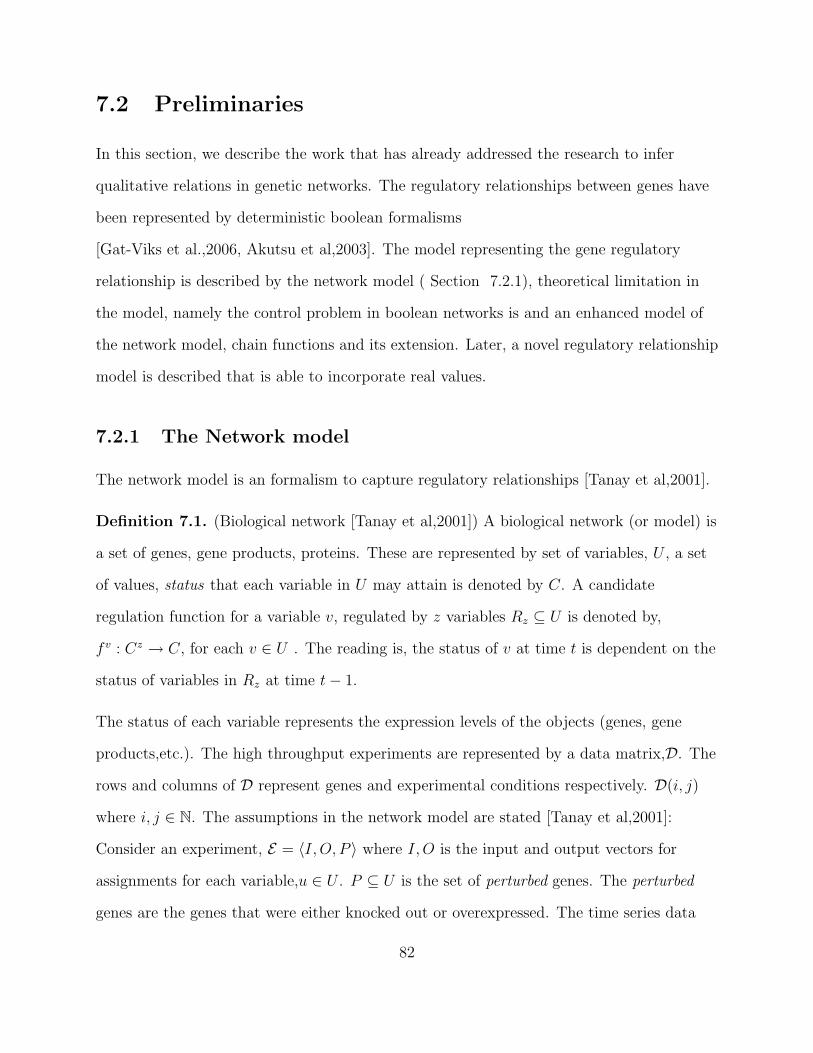
7.2 Preliminaries

In this section, we describe the work that has already addressed the research to infer

qualitative relations in genetic networks. The regulatory relationships between genes have

been represented by deterministic boolean formalisms

[Gat-Viks et al.,2006, Akutsu et al,2003]. The model representing the gene regulatory

relationship is described by the network model ( Section 7.2.1), theoretical limitation in

the model, namely the control problem in boolean networks is and an enhanced model of

the network model, chain functions and its extension. Later, a novel regulatory relationship

model is described that is able to incorporate real values.

7.2.1 The Network model

The network model is an formalism to capture regulatory relationships [Tanay et al,2001].

Definition 7.1. (Biological network [Tanay et al,2001]) A biological network (or model) is

a set of genes, gene products, proteins. These are represented by set of variables, U , a set

of values, status that each variable in U may attain is denoted by C. A candidate

regulation function for a variable v, regulated by z variables Rz ⊆ U is denoted by,

f v : Cz → C, for each v ∈ U . The reading is, the status of v at time t is dependent on the

status of variables in Rz at time t− 1.

The status of each variable represents the expression levels of the objects (genes, gene

products,etc.). The high throughput experiments are represented by a data matrix,D. The

rows and columns of D represent genes and experimental conditions respectively. D(i, j)

where i, j ∈ N. The assumptions in the network model are stated [Tanay et al,2001]:

Consider an experiment, E = 〈I, O, P 〉 where I, O is the input and output vectors for

assignments for each variable,u ∈ U . P ⊆ U is the set of perturbed genes. The perturbed

genes are the genes that were either knocked out or overexpressed. The time series data

82

representing expression levels for a series of n time points and yield n− 1

experiments(triples). An experiment having I = O is a steady state experiment. Steady

state experiments exclude the case in the the model where variables regulate themselves

(hence eliminate self regulation). The data in steady state eliminates the requirement for

additional synchrony assumptions (time series data is along some sychronized biological

process).

The model provides the likely networks containing,P for given I and O. The limitation of

the network model is that it is computationally expensive [Tanay et al,2001]. The network

model lays the foundation for boolean formalism addressing the problem of inferring

genetic relationships from experimental data,mainly gene expression data.

7.2.2 The Control problem

In biology, there may be several factors influence genes during regulation. Identification of

a set of perturbations and its effects on the system is important to understand complex

biological system. Hence, the need of a control theory on biological systems had been

addressed [Kitano,2002] for a system level understanding of biological processes relate it to

the set of perturbations that affects biological behaviors. The results from control theory

model linear systems but they fail when applied to nonlinear biological systems. A way to

incorporate the influence of other genes or factors is by defining a control bit for a gene. In

the case of boolean model, the control bit has a boolean value. Prior work using boolean

networks to model genes and their expression levels have been reported [Kauffman,1993]. A

boolean network is a directed graph G(V, F ) where V represents a set of nodes and F , a set

of boolean functions. In a boolean network model of a genetic network the nodes represent

gene or gene products. Each node is labeled a boolean value and the value of the nodes

change synchronously with a discrete value of time, t. The boolean function assigns value

to the node, na ∈ V for the next step with other nodes that influence na. The control

83

problem associated with the boolean network occurs when m external nodes, 〈u1, . . . , um〉

are added to the n original(internal) nodes, 〈v1, . . . , vn〉 of the boolean network. The value

of any internal nodes, vi is controlled by a subset, C = of the set of external and internal

nodes. vi at time t+ 1 is given by the equation vi(t+ 1) = fi(C)(t) where fi is the boolean

function. The vector, V k = 〈v1(k), . . . , vm(k)〉 represents the boolean values of the internal

nodes in the kth. time step. Similar notation for the values of external nodes at time step

k is, xk = 〈u1(k), . . . um(k)〉.

Definition 7.2. (Boolean-network(BN) control problem [Akutsu et al.,2007]) A boolean

network (BN) is a directed graph, G(V,E) with boolean functions defined on each v ∈ V .

Given an initial state of vertices of G represented by a boolean vector, V 0 and the desired

state on the vertices after mth. time steps represented by a boolean, V p. The BN-control

problem is to find values of the external nodes 〈x0, . . . xp〉 such that V (0) = V 0 and

V (p) = V p. If there does not exist such a set, the output should be “No”.

Theorem 7.1. ([Akutsu et al.,2007]) BN-Control is NP-hard.

The use of boolean control vector is a mechanism to reduce complexity of the number of

degree of freedom of influences on the regulator set.

7.2.3 Chain functions

A boolean formalism incorporating the control property of the genes called chain functions

have been reported. Earlier,a boolean model to identify genetic network was proposed by

Akustu et al [Akutsu et al,2003] and later, was enhanced by chain function model

[Gat-Viks et al.,2006]. We review the chain function model [Gat-Viks et al.,2006]. The

chain function model [Gat-Viks et al.,2006] have additional conditions to that of the

network model: (i) the status of variables are assumed to discrete and take only boolean

values. (ii) the regulatory relations are deterministic. Before formally defining chain

84

function, we introduce the following notation [Gat-Viks et al.,2006]. A set of variables is

denoted U where the variables represents genes and gene products. Also, | U |= n+ 1 ,

n ∈ N. A status of a variable(gene), g ∈ U represents a boolean value and is given by

sta : g → {0, 1}. The sta(g) is the boolean value of the expression level of a gene, g. Any

perturbations on a variable changes its status. A chain function can be described, quoting

[Gat-Viks et al.,2006]:

A variable, g0 ∈ U is regulated by U1 = {g1, g2, . . . , gn} ⊂ U , if there is a

function, f g0 such that sta(g0) = f g0(sta(gn), . . . , sta(g1)) and U1 is minimal set

with that property.

The function, f g0 is the chain function for g0 for a set of regulator set, U1. The set, U1 is

the regulator set and g0 is the regulatee. The control property for each gi ∈ U1 where

1 ≤ i ≤| U1 | is given by binary constant,yi. If yi = 0(1), gi is an activator (repressor). The

control property is static for the set of regulator. The status of the regulatee, g0 depends

on the chain function, f g0 on the set of regulators, U1. The function, f g0 is defined by two

n-dimensional vectors, a(gi) and in(gi) representing the activity and influences to each

gi ∈ U1. The influence, in(gi) represents the influence of gi on gi−1. An ordering defined on

the set, U sta1 = {sta(gn), . . . , sta(g1)} implies sta(gi) is the successor of sta(gj) i < j.

The algorithm to compute sta(g0) given by [Gat-Viks et al.,2006]:

Algorithm 2 ChainFunction(g0,U sta1 , Y )

Input: Regulatee,g0,Status of the genes in the ordered set of regulators,U sta1

Control pattern of the regulators,Y = {yn, . . . , y1}Output: Status of Regulatee,sta(g0).1: Initialize in(gn+1) = 1. // in(gn) is the influence on gn is always 1.2: for j → n to 1 do3: a(gj) = in(gj+1) ∧ sta(gj). // a(gn) represents the activity of gn.)4: in(gj) = yj ⊕ a(gj).5: end for6: sta(g0) = in(g1)

85

The total number of boolean functions for m variables is Θ(22m). By contrast, chain

function formalism [Gat-Viks et al.,2003] is computationally efficient.

Theorem 7.2. ([Gat-Viks et al.,2003]) The number of chain functions with m control

variables is Θ(m!(log2e)m+1).

7.2.4 Regulatory Relationship Model

In this section, we describe our formalism of gene regulation. We use the intuition that a

set of genes, regulatee is regulated by another set of genes, regulators . The set of

regulators does not change its expression levels during the process of regulation. Each

regulatee changes its expression levels.

A regulatory relationship capturing regulatee-regulator relationship is represented by a

formula

{l1(g1), l2(g2) . . . , lm(gm)}{l1(g′1),...,lk(g′k)}−→ {l1(g1), l2(g2), . . . , lm(gm)}

where m, k are positive integers, gm’s and g′k’s are genes forming regulatees and regulators.

The reading is that gene g1 changes its expression level from l1 to l1, gene g2 changes its

expression level from l2 to l2,· · · and gene gm changes its expression level from lm to lm in

the presence of set of regulators given by gene g′1 with expression level l1,· · · and gene g′k

with expression level lk.

Formally, we define a regulation for a regulatory relationship in the following way:

We are given a set of genes, G, set of labels representing the expression levels of the genes,

El , a labeling function, L : G ⊆ G → El represents genes labeled with expression levels.

(Notation, LG means labelling funtion L on a set of genes, G)

Definition 7.3. (Regulation) A regulation, Reg = 〈LG, LG, LG′〉 such that:

86

1. (Change in Expression Level) LG ∩ LG = ∅ where L, L are the labeling functions

representing the expression levels on a set of genes, G before and after the regulation

respectively.

2. (Disjoint Condition) G ∩G′ = ∅ and G 6= ∅.

3. (Minimality) There is no set, LG ⊂ LG′ such that there is a regulation,

Reg′ = 〈LG, LG, LG〉. Here, L is the labeling function on the set of regulators,G′.

The regulatory-relationship formalism captures the notion of boolean values where presence

of a gene with a specific label may be true/false. Also, this formalism does not assume the

knowledge of the control vectors and is data-dependent. The labeling on the genes models

the experimental data. A gene, ga with expression label, x regulates another gene, gb with

expression label, y. Here, the labels on the ga and gb will be x and y ,respectively.

Example 7.1. (Representations of regulations) The regulatory relationships that can be

captured with our definition of regulation in the case of transcription(TF)-DNA

interactions are explained. Network motifs model interactions and are represented by a

directed graph where the nodes are labeled with transcription factors and genes. The

direction on the edges represent direction of the regulaton (translational and binding

activity as shown in the Figure 7.1 by a transcription factor [Blais et. al.,2005] on gene. In

our definition, TF proteins, TF-encoding gene and target genes are represented as set of

labelled genes. Using definition and notation of regulation, we show network motifs are

modeled by our formalism.

We describe the different ways of regulations with our formal definition of regulation.

Recall, the set representing regulatee, LG after regulation becomes LG and the set of

regulator is represented by LG′ . In some cases of this example shown in Figure 7.1, LG is

unknown because the expression levels after the regulation is not mentioned.

1. Auto-regulation: The transcription protein and the TF-encoding gene are represented

87

Figure 7.1: Transcriptional regulatory network motifs [Blais et. al.,2005]

88

by LG and LG respectively. Here, the set of regulators, LG′ = ∅. Note, our definition

of regulation differs from Gat-Viks model [Gat-Viks et al.,2006]. The Gat-Viks model

assumes that set of regulators is a nonempty set, hence,the model does not express

auto regulation.

2. Feed Forward Loop: In our formalism, we represent the feed forward loop by using

two distinct regulations,respectively.

(a) The first regulation,reg1 is modeled by: 〈LG, LG, LG′〉 represents TF2 encoding

gene, TF2 protein and TF1.

(b) In the second regulation, LG, LG′ represents target gene and combined set( TF1

protein and TF2 protein). In this regulation the LG is not mentioned that is

expression level of the target gene after the regulation.

3. Multi-component Loop: The multi-component loop is represented by two regulations.

(a) The first regulation, LG, LG and LG′

represent TF2 (TF-encoding gene),TF2

(TF protein) and TF1 respectively.

(b) The second regulation,LG, LG and LG′

represent TF1,TF1-protein and TF2

protein,respectively.

In the multi-component loop,the second regulation triggers the first and vice versa.

4. Regulator Chain: In this network motif,there are three regulations that are ordered:

(a) First regulation: LG, LG and LG′

represent TF2 encoding gene,TF2 protein and

TF1 protein respectively.

(b) Second regulation: LG, LG and LG′

represent TF3 ending gene protein, TF3

protein and TF2 protein respectively.

(c) Third regulation: LG and LG′

represent target gene and TF3 protein respectively.

Here , LG is the expression level of the target gene is not mentioned.

89

5. Input- based network motifs: There are two types of input based network motifs. In

each case, LG is not shown in the Figure 7.1:

(a) Single Input: LG and LG′

represent target gene and TF respectively.

(b) Multiple Input: LG and LG′

represent target gene and combination of TF1,TF2

and TF3, respectively. Note: LG′

an be either of TF1,TF2 or TF3 only, taken

two TFs at a time. In each case the regulation would be different.

7.3 Kripke structure representing regulatory

relationship

We are given (1) a set of genes,G (2) for each gene g ∈ G a set of labels, El representing the

expression levels, for el ∈ El, el ∈ R (3) a set of regulations,Reg and a set of labeling

functions,L. We define the Kripke structure,M = 〈S,R, L〉 (refer to chapter 1 for the

defintion) in the following way:

• AP is the set of all the atomic formulas of the form l(g) = 0 or l(g) = el where l ∈ L

and g ∈ G. (Notation: l(g) are symbols representing the expression level of a gene, g.)

• S is the set of subsets s of AP where, for each g ∈ G, exactly one of the formulas of

the form, l(g) = 0 or l(g) = el is in s.

For such a state s, L(s) = s, i.e., L “says” that every atomic formula in s is true and

that all others are false. The states contain expression levels of the genes in the

system.

• For all s, s′ ∈ S and a regulatory relationship given by

{l1(g1), l2(g2) . . . , lm(gm)}{l1(g′1),...,lk(g′k)}−→ {l1(g1), l2(g2), . . . , lm(gm)}

90

is represented by reg ∈ Reg. The notation for the set of regulatee before and after

regulation ,reg is LG and LG, set of regulators in given by LG′ where L, L, L ∈ L.

Here, LG means L ∈ L is a labeling function on a set of gene,G. Also,

G ⊆ G, G′ ⊆ G \G. Symbolically, a regulation is LGLG′−→ LG. We use the

notation:s(l(g)) means gene,g ∈ G with expression level l(g) true in state s ∈ S.

l(g), l(g) represents any of the genes labeled with expression levels in the regulatee

before and after the regulation respectively. l(g) is the any genes with expression

level from the set of regulators. There is an edge from s to s′ representing a

regulation if ∃x, y ∈ R

1. ∀lg ∈ LG, x ∈ s(lg).

2. ∀lg ∈ LG, y ∈ s′(lg).

3. ∀lg′ ∈ LG′ , s(lg′) = s′(lg′).

4. ∀lg ∈ LG\G, s(lg) = s′(lg) where L ∈ L.

7.4 Application of the Regulatory-Relation to

Galactose Utilization Pathway in Yeast

The regulatory-relationship formalism captures the notion of boolean values where presence

of a gene with a specific label may be true/ false. Also, this formalism does not assume the

knowledge of the control vectors and is data-dependent. The labeling on the genes models

the experimental data. A gene, ga with expression label, x regulates another gene, gb with

expression label, y. Here, the labels on the ga and gb will be x and y ,respectively.

91

7.4.1 Galactose Utilization Pathway

The function of galactose(gal) pathway is to transport galactose in a cell and then

efficiently convert into glucose-6-phosphate [Idekar et al.,2001]. Galactose is transported in

the cell by GAL2 or HXT . The enzymes, GAL1, GAL7, GAL10, GAL5 convert convert

galactose to galactose-1-P and finally, glucose-6-phosphate is formed. The regulatory

network for the gal pathway consists of GAL4, GAL80 and GAL3 for the trancriptional

control of the transportation of galactose and conversion of galactose into

glucose-6-phosphate. The function of GAL6 is not known clearly. The gal pathway is

shown in the Figure 7.2 is adapted from [Idekar et al.,2001]. Figure 7.2 shows the

processes from the galactose pathway that are moldeled in our formalisms.

The representation of the Gal pathway is given by the following relations. The notationx↔

represents “in the presence of x”.

7.4.2 Regulatory Relationship Model of the Galactose Pathway

We assume to gene and proteins as entities participating in the gal utilization pathway.

The notation for the labels representing the expression levels on the genes before and after

the regulation is given by L and L The gal pathway represented in the

regulatory-relationship model for the gal pathway is given below:

1. Metabolic Pathway

(a) LG(GAL)L2(GAL2)/HSTs←→ LG(GAL).

(b) LG(GAL),LGP (GAL1P)L1(GAL1)←→ LGP (GAL1P),LG(GAL).

(c) LGP (GAL1P),LGL1(GL1P)L7(GAL7)←→ LGL1(GL1P),LGP (GAL1P).

(d) LGL1(GL1P),LGL6(GL6P)L5(GAL5)←→ LGL1(GL1P),LGL6(GL6P).

2. Regulatory Network

92

Figure 7.2: Galactose Pathway (adapted from [Idekar et al.,2001])

93

(a) L2(GAL1)x←→ L2(GAL1),where x = L3(GAL3), L4(GAL4), L80(GAL80).

(b) L7(GAL7)x←→ L7(GAL7),where x = L3(GAL3), L4(GAL4), L80(GAL80).

(c) L5(GAL5)x←→ L5(GAL5),,where x = L3(GAL3), L4(GAL4), L80(GAL80).

The aforementioned relationships are the system constructs for probabilistic model

checking. We outline the probabilistic model for the galactose pathway using the

relationship regulation model.

7.4.3 Noise in Gene Expression

Gene expression have been described as a stochastic process

[Swain et al.,2002, Elowitz et al.,2002]. The stochastic fluctuations in cellular components

are significant. It is explained by intrinsic (ηint) and extrinsic (ηext) noise. The stochastic

property of gene expression is explained from [Swain et al.,2002].

Stochasticity in Gene expression

Paraphrasing from [Swain et al.,2002]:

Translation and transcription are triggered at different times and different

orders in different cells and are caused by gene sequence and properties of the

encoded protein. These stochastic perturbations occur locally and caused by

gene sequence and properties of the encoded protein and are referred “intrinsic”

noise . Extrinsic noise occurs due to fluctuations in the gene expression caused

by the other molecular species in the cell such as RNA polymerase. The protein

noise , η(t) and protein concentration,P (t) at time t given by the following

mathematical formula:

η2(t) =〈P (t)2〉 − 〈P (t)〉2

〈P (t)〉2

94

where the angled brackets denote an average over the probability distribution of

P at time t.

The total experimentally measurable noise,ηtot is given by [Swain et al.,2002]:

η2tot = η2

int + η2ext. Recent work [Collins et al.,2010] have illustrated a way to tune and

control gene expression noise by designing biological experiments that TATA box (segment

of DNA sequence found in the promoter of a gene) mutations and noise propogation during

transcription. The experimental data was validated by a numerical mathematical model to

capture noise in the gene expression data. Stochastic boolean model [Garg et al.,2009] have

reported overpresentation of noise in gene regulatory networks.

7.4.4 Model Construction

The perturbation matrix data from the galactose perturbation experiments are used for the

contruction of the model.

Modeling noise in the model: We collect all the regulatory relations of the form

Lg1LG−→ Lg1 . There is a regulation if there is a change of the expression levels of a gene in

an experiment (such as gene knock-out experiments) from its wildtype level. We model

noise in the experiments by representing probabilities on the transitions. For example for

the regulation,Lg1LG−→ Lg1 , let Lg1 = 1, Lg1 = 2.3. We represent multiple values of Lg1 to

accomodate noise in the model. Therefore for the regulation,Lg1LG−→ Lg1 is represented by

the three transitions, Lg1LG−→ Lg1 = 2.2, Lg1

LG−→ Lg1 = 2.3 and Lg1LG−→ Lg1 = 2.4 with

probability of .2,.6 and .2,respectively.

Construction of Gene Network: The relationships between the regulation relations is

derived recursively. An example of the regulations relations is given by

Lg1Lg2−→ Lg1 .

Lg2Lg3−→ Lg2 .

95

Lg3Lg4−→ Lg3 .

. . .

Lgn

Lgn−1−→ Lgn .

Hence, the regulation in a recursive way and the interaction is shown in a form of a path,

πregulation = gn, gn−1 . . . g1. Clearly, the paths can be non-deterministic if the

regulatee/regulator are set of labeled genes and for each lalebed gene in the sets, a path

πregulation can be constructed.

7.4.5 Simulation

We implement the model in PRISM (www.prismmodelchecker.com) on a Sun machine with

processor of 502 Mhz with 1152 MB memory. Idekar date set [Idekar et al.,2001] is used for

the simulation the regulatory relationship formalism. The stochastic models that are used

in the modeling are discrete time markov chain and markov decision processes. The

probabilistic temporal logic queries are in PCTL logics. We pose sample PCTL queries and

record the times. The intervals are representation of the gene expression levels. Stated in

the section 7.3, the labels,el are in the form of (a1, a2]. The intervals are represent

expression levels such as high, low and medium. The regulatee-regulator is constructed

from the data whenever there is a change in expression value from the wildtype (normal)

level. Figure 7.3 shows the formalism is based on discrete time markov chain (DTMC) and

markov decision process (MDP). We assume that the probabilities on the transitions of an

indentical distribution is equally likely. In the simulation model, the stochastic formalisms

represent the noise in the data. The DTMC model is deterministic in terms of probability

distribution labeled on the transitions from a state. The MDP model introduces

nondeterminism in the model and selects nondeterministically the probability distribution

from a state. Clearly, DTMC representation of regulatory relationship than the MDP

96

representation. Figure 7.3(A) shows the discrete time markov chain model for the

regulatory relationship. g3(l3) acts as a trigger to gene, g1 and g2 with labels l1, l2,

respectively. The probabilities, p is 1/4. Figure 7.3(B) represents the markov decision

model for the regulatory relationship where the probabilities, p1 and p2 are 1/3 and 1/2

respectively. p1 and p2 represent different distributions.

Figure 7.3: Representation of regulatory relationship in stochastic formalisms.

7.4.6 Results from simulation of Galactose Pathway

We pose simple PCTL (probabilistic CTL)logic on DTMC and MDP formalisms of

regulatory relationship record the times.

The sample PCTL queries (for expression level high) are the following:

Query 1-2: The maximum probability to reach a state where GENE is at level,high. PCTL

formula, Pmax? = (trueUGENE = high)

Query 3-4: The probability that GENE is at level high is less than .1. PCTL formula,

P<0.1(FGENE = high)

97

Query 4-6: The probability that GENE is at high is within 7 steps from GENE is in its

wildtype state is atleast 0.98. PCTL formula,

P≥0.98[(GENE = wildtype)U<=7(GENE = high)].

Query 7-8: From an initial state, the probability that GENE is in wildtype state before it

expresses to high level is greater than equal to 0.99. PCTL formula,

”init” => P≥0.99[(GENE = wildtype)U(GENE = high)]

Query PCTL formula Number of IntervalsDTMC(in sec) MDP (in sec)5 8 10 15 5 8 10 15

1. Pmax? = (trueUGAL1 = high) 0.077 1.24 1.281 12.384 0.983 54.266 142.57 -2. Pmax? = (trueUGAL6 = high) 0.006 0.045 0.064 0.143 0.007 0.041 0.064 -3. P<0.1(FGAL1 = high) 0.144 4.9 4.92 51.36 1.737 227.79 1073 -4. P<0.1(FGAL1 = high) 0.002 0.003 0.003 0.005 0.002 0.002 0.029 -

5. P≥0.98[(GAL7 = wildtype)U<=7(GAL7 = high)] 0.078 2.7 2.382 25 1.774 199.06 805 -

6. P≥0.98[(GAL3 = wildtype)U<=7(GAL3 = high)] 0.002 1.8 1.763 19 0.002 183.85 774 -

7. ”init” => P≥0.99[(GAL1 = wildtype)U(GAL1 = high)] 0.097 2.8 2.967 29.57 1.638 209.218 837 -

8. ”init” => P≥0.99[(GAL6 = wildtype)U(GAL7 = high)] 0.002 2.2 2.259 24.42 0.002 188.633 792 -

Table 7.1: Execution times(in seconds) for PCTL queries on a regulatory relationship con-struction using galactose dataset [Idekar et al.,2001] .”-” represents greater than 20 minutes.

7.5 Discussion

In this work, we formalize regulatory relationship and automate the construction of gene

regulatory relationship taking account of noise in the data. We simulate the theoretical

formalism using the galactose dataset. The simulation supports the fact that non

deterministic formalism is computationally intensive on the prototype constructed from

galactose dataset. The accuracy for the construction of galactose pathway is proportional

inversely to the computational effciency of the regulatory relationship formalism. The

regulatory relationship formalism provides insights for automated construction of gene

regulatory relationships from noisy data. Hence, the need to investigate for an efficient

stochastic formalism that is data dependent is of paramount importance. One way is to

construct markov decision processes and then, a probability distribution, D is constructed

98

from data. Clearly, the probability distribution D eliminates the nondeterminism and is

data dependent, call the formalism, mixture of markov models. The temporal logics for

mixture of markov models is to be investigated further.

99

Chapter 8

Future work

The dissertation addresses some of the important modeling problems in large scale systems

with applications in systems biology.

First, model abstractions and several algorithms were created to incorporate incomplete

and imprecise knowledge in the model. Second, the definition of multiscale formalism in

discrete domains are stated and a polynomial time complexity algorithm is constructed to

compute equivalences in two transition systems representing multiscale processes. Third, a

formalism, using probabilistic system modeling and automated reconstruction of gene

regulation relationships incorporating noise from the biological experimental data, is

created.

When I think about the future work in the domain of fomal analysis and model

abstraction, I envision three significant bodies of work based on the work from this

dissertation. Each of the topics would require overlapping knowledge but can be

”stand-alone” by itself. I want to describe how the results of this dissertation will form the

foundation for the three research directions.

1. Modeling of Chemical Reactions: In this dissertation, the modeling of chemical reactions

addressed the imprecise and incomplete knowledge. Biochemical modeling in general is

100

multiscale. It is natural to integrate multiscale formalism with imprecise and incomplete

knowledge in biochemical modeling. The model abstraction will borrow ideas from

chapters on chemical reaction modeling and multiscale formalism. The integrated model

will be rigorously validated with biological experimental data in different pathways.

2. Formal Analysis Large Scale System Models: We addressed multiscale formalism. The

theoretical research questions are as follows:

1. Is there a sublinear algorithm to compute the equivalences?

2. Is there a definition of multiscale formalism in probabilistic system modeling?

3. Use the ideas developed in the multiscale formalism and seek a solution for the

identifiability problem of hidden markov model [Blackwell et al.,1957].

The solution to the aforementioned queries would have significant contributions in the

foundations of formal analysis of multiscale systems.

3. Temporal Logics on Mixture of Stochastic Models: The gene network modeling provided

us some insights of modeling data with noise. The current probabilistic logics that are

published are on markov chains, markov decision models and continuous time markov

model. Temporal logic formalism on a mixture of stochastic models has not been addressed

till date. The advantages of mixture of markov chains is its ability to incorporate

uncertainty in the selection of the markov chain. It will be also be more data dependent

such that probabilities assigned to select the markov chain. The theory of temporal logics

for the mixture of markov chain will be formalized in future.

Summary: I gave an outline for some of the immediate future research directions. There

are innumerous research areas in which formal modeling can be applied. I feel, in the area

of formal modeling, we have just broken the ground to build a strong foundations for a

massive structure. One of the active research areas is the intersection of embedded systems

101

and human computer interaction. Another research area is temporal reasoning of clinical

records under uncertainty. The list is endless and clearly, illustrates the potential of formal

modeling in several research areas in computer science. The challenge in foreseeable future

is to bridge the gap between what we can contribute and what we would want to

accomplish in the area of formal modeling.

102

Bibliography

[Kitano,2002a] Kitano,H. Systems biology: A brief overview,Science,2002,Vol. 295,no.

5560,pp 1662-1664.

[Kitano,2002b] Kitano,H. Computational systems biology Nature,2002,420,206-210.

[Lesser,2005] Leser,U A query language for biological networks,Bioinformatics, Sep 1;21

Suppl 2:ii33-ii39 ,2005.

[Krishnamurthy et al.,2003] Krishnamurthy,L., Nadeau1,J., G. Ozsoyoglu,G.,

Ozsoyoglu,M.,Schaeffer,G., Tasan,M. and Xu,W.Pathways database system: an

integrated system for biological pathways,Vol. 19,pp 930-937,Bioinformatics,2003.

[Clarke et al.,1986] Clarke,E.,M.,Grumberg,O. and Peled,D.,A. Model Checking, The MIT

Press,1999.

[Pneuli,1981] Pneuli,A .A temporal logic of programs Theoretical Computer

Science,13:45-60,1981.

[Cooper et al,2009] Cooper,G. and Hausman,R. The Cell : A Molecular Approach, Fifth

Edition.

[Manna et al.,1991] Manna,Z. and Pnuelli,A. The Temporal Logic of Reactive and

Concurrent Systems,Publisher Springer Verlag,1991.

103

[Clarke et al.,1983] Clarke,E.,M.,Emerson,E.,A and Sistla,A.,P. Automatic verification of

finite-state concurrent systems using temporal logic specifications Proceedings of the

10th. Annual ACM Symposium on Principles of Programming Language,1983.

[Sistla et al.,1985] Sistla, A. P., and Clarke, E. M. Complexity of propositional linear

temporal logics, J. ACM 32,3 , 733-749,1985.

[Kifer et al.,1992] Kifer,M and Subrahmanium,V.,S. Theory of Generalised Annotated Logic

Programing and its Application, Journal of Logic Programming,12,4 pp 334-368,1992.

[Langmead et al,2006] Langmead,C.,L.,Jha,S. and Clarke,E.,M. Temporal Logics as query

languages for dynamic bayesian networks: Application to D. Melanogaster embryo

development,Carnegie Mellon School of Computer Science Technical

report,CMU-CS-06-159,September 2006.

[Temkin et al.,1996] Temkin,O.,N.,Zeigarnik,A.,V. and Broncheev,D. Chemical Reaction

Networks, A Graph-Theoretical Approach CRC Press,1996.

[Benko et al.,1999] Benko,G, Flamm,C., and Stadler,P.,F. A Graph-Based Toy Model of

Chemistry Journal of Chemistry Information and Computer Science.

[Eker et al.,2002] Eker,S.Knapp,M.,Laderoute,K. Lincoln,P.,Meseguer,J. and Sommez,K.

Pathway logic:symbolic analysis of biological signaling, Pacific Symposium on

Biocomputing 2002(PSB 2002),2002.

[Rivier-Chabrier et al.,2004] Rivier-Chabrier,N.,Chiaverini,M.,Danos,V.,Fages,F.,Schacter

Modeling and query biomolecular interaction networks ,Theoretical Computer

Science,25-44,325,2004.

[Fisher et al.,2008] Fisher,J. et al Bounded Asyncrony: A biologically notion of

concurrency,Proceedings of FMSB,2008,Cambridge,Springer.

104

[Lamport,1983] Lamport,L What good is temporal logic, Information Processing 83,R.E.A

Mason,editor,Elsevier Publications,1983,657-688.

[Alur et al.,2001] Alur,R. ,Belta,C.,Ivancic,F.,Kumar,V.,Mintz,M., Pap- pas,G.,J,Rubin,H.

and Schug,J. Hybrid modeling and simulation of biomolecular networks. Lecture Notes

in Computer Science, 2034, 2001.

[Shrivats et al.,2005] Shrivaths,R. and Prasad,S. Verifying Dynamics for Biochemical

Systems,ICSB,2005.

[Faeder et al.,2005] Faeder,J.,R., Blinov,M.,L.,Goldstein,B. and Hlavacek,W.,S. Rule based

Modeling of Biochemical Networks Complexity,Complexity, 10, 22-41,2005.

[Antoiotta et al.,2004] Antoniottia,M.,Piazza,C.,Policritid,A., Simeonic,M and Mishra,B.

Taming the complexity of biochemical models through bisimulation and collapsing:

theory and practice, Theoretical Computer Science,325,45-67,2004.

[Antoiotta et al.,2003] Antoniottia,M.,Piazza,C.,Policritid,A., Simeonic,M and Mishra,B.

Model building and Model checking of Biological Processes,Cell Biochemical and

Biophysics,38(3),272-286, 2003.

[Ciobanu,2004] Ciobanu,G. Software verification of biomolecular systems. In G.Ciobanu,

G.Rozenberg (Eds.): Modelling in Molecular Biology, Natural Computing Series,

Springer, 40-59, 2004.

[Bockmayr et al.,2002] Bockmayr,A. and Courtois,A. Using hybrid concurrent constraint

programming to model dynamic biological system ICLP,2002.

[Calzone et al.,2006] Calzone,L,Fages,F and Soliman,S. BIOCHAM: an environment for

modeling biological systems and formalizing experimental knowledge,Bioinformatics Vol.

22, no. 14., pages 18051807,2006.

105

[Ausiello et al.,1983] Ausiello,G.,D’Atri,A. and Sacca,D. Graph algorithms for functional

dependency, Journal of ACM,30:752-766,1983.

[Yadav et al.,2004] Yadav,M.,Kelley,B.,P.,Silverman,S.,M. The Potential of a Chemical

Graph Transformation System H. Ehrig et al. (Eds.): ICGT 2004, LNCS 3256, pp.

8395, 2004.

[Rosello et al.,2004a] Rosello,F. and Valiente,G.Chemical Graphs, Chemical Reaction

Graphs and Chemical Graph Transformation, GraBaTs ,2004 Preliminary version.

[Vardi,2005] Vardi,M.,Y. Model Checking for Database Theoreticians ,T. Eiter and L.

Libkin,Editore: ICDT 2005, LNCS 3363, pp. 116, 2005.

[Rosello et al.,2004] Rosello,F. and Valiente,G.Analysis of Metabolic Pathways by Graph

Transformation, H. Ehrig et al. (Eds.): ICGT 2004, LNCS 3256, pp. 7082, 2004.

[Gallo et al.,1993] Gallo,G. et al. Directed Hyper-graphs and Applications, Discrete

Applied Mathematics, Vol. 42, pp. 17720,1993.

[Aziz et al.,1995] Aziz,A.,Singhal,V., Balarin,F., Brayton,R.,K. and

Sangiovanni-Vincentelli,A. It Usually Works: The Temporal Logic of Stochastic Systems

Proceedings of Conference on Computer-Aided Verification, Liege, Belgium, July, 1995.

[Hansson et al.,1994] Hansson,H. and Jonsson,B. A Logic for Reasoning about Time and

Reliability,Formal Aspects of Computing ,6, pp. 512-535,1994.

[Hermanns,2002] Hermanns,H. Interactive Markov Chains and the Quest for Quantified

Quality,Lecture Notes in Springer Verlag,2002.

[Kemeny et al.,1966] Kemeny,J.,Snell,J. AND Knapp.A. Denumerable Markov Chains, D

.Van Nostrad Company,1966.

106

[Baier et al.,2002] Baier,C. and Kwiatkowska,M. Model checking for a probabilistic

branching time logic with fairness. Distributed Computing,11(3):125-155,1998.

[Courcoubetis et al.,1988] Courcoubetis,C. and Yannakakis,M. Verifying temporal

properties of finite state probabilistic programs, Proceeding of FOCS,pp. 338-345, IEEE

computer Society Press,1988.

[Courcoubetis et al.,1990] Courcoubetis,C. and Yannakakis, M. The complexity of

probabilistic veridication. Journal of the ACM,42(4),857-907,1995.

[Chatterjee et al.,2003] Chatterjee,Dasgupta,P. and Chakrabarti,P.,P. A Branching Time

Temporal Framework for Quantitave Reasoning, Journal of Automated Reasoning,

30,205-232,2003.

[Batt et al.,2005] Batt,G.,RoperS,d,de Jong,H.,Geiselmann,J. Mateescu,R., Page,M. and

Schneider,D. Validation of qualitative models of genetic regulatory networks by model

checking: analysis of the nutritional stress response in Escherichia coli,

Bioinformatics,Vol 21, Suppl 1,pp i19-i28,2005.

[Batt et al.,2007] Batt,G. Belta,C. and Weiss,R. Model checking genetic regulatory

networks with parameter uncertainty, Tenth International Workshop on Hybrid

Systems: Computation and Control,HSCC’07, Editors. A.Bemporad,A Bicci and

G,Butazzo,Lecture Notes in Computer Science 4416,Springer-Verlag,61-75.

[Thorsley et al.,2010] Thorsley,D. and Klavins,E. Theory of Approximation for Stochastic

Biochemical Processes,Control Theory and Systems Biology, edited by Iglesias,P,.A and

Ingalis,B.P, MIT Press, 2010.

[Bernot et al.,2004] Bernot,G.,Comet,J.,Richard,A. and Guespin,J. Application of formal

methods to biological regulatory networks extending Thomas’ asynchronous logical

approach with temporal logic, Journal of Theoretical Biology,229,2004.

107

[Lander et al.,2001] Lander,E. et al, Initial sequencing and analysis of the human genome.

Nature 409,6822,2001.

[Baltimore,2001] Baltimore,D. Our genome unvieled Nature 409, 6822,814-816.

[Emerson et al.,1992] Emerson,E.,A,Mok,A.,K,Sistla,A.,P and Srinivasan,J. Quantative

Temporal Reasoning Real-Time,4,331-352.

[Castellan,1983] Castellan ,G.,W. Physical Chemistry, Third Edition, Addison Wesley

Publisher 1983.

[Levine,2002] Levine,I. Physical Chemistry, Fifth Edition, McGraw-Hill Higher Education,

2002.

[Schuab et al.,2007] Schaub M.,A., Henzinger, T.,A., Fisher J. Qualitative Networks: A

Symbolic Approach to Analyze Biological Signaling Networks, BMC Systems Biology.

1:4, 2007.

[Fisher et al.,2006] Fisher,J. and Henzinger,T.,A. Executable biology, Proceedings of the

Winter Simulation Conference (WSC), IEEE Computer Society Press, 2006.

[Baral et al.,2004] Baral,C.,Chanceller,K.,Tran,N.,Tran,N.,L.,Joy,A. and Berens,M. A

knowledge based approach for representing and reasoning about signaling

networks,Bioinformatics, Vol. 20, Supplement1,pp. i15-i22,2004

[Priami,2003] Priami,C.(ed.) Computational Methods in Systems Biology, LNCS 2602,

Springer Verlag, 2002.

[Parker,2002] Parker,D. Implementation of Symbolic Model Checking for Probabilistic

Systems,Ph.D. thesis, University of Birmingham. August 2002.

108

[Talcott et al.,2004] Talcott,C., Eker,S., Knapp,M.,Lincoln,P. and Laderoute,K. Pathway

logic modelling of protein functional domains in signal transduction,Pacific Symposium

on Biocomputing 2004 (PSB 2004),pp 568-580.

[Ghosh et al.,2004] Ghosh, R. and Tomlin, C. Symbolic reachable set computation of

piecewise affine hybrid automata and its application to biological modelling: Delta-notch

protein signalling, Systems Biology, 1(1):170183, June 2004.

[Regev et al.,2001] Regev,A.,Silverman,W., Shapiro,E.,Y. Representation and Simulation

of Biochemical Processes Using the pi-Calculus Process Algebra, Pacific Symposium on

Biocomputing, 459-470,2001.

[Clarke et al.,1986] Clarke,E.,Emerson,E.,A. and Sistla,A.,P. Automatic Verification of

Finite State Concurrent Systems using Temporal logic specifications,ACM Trans. of

Programming Languages and systems:8(2):244-263,April,1986.

[Kwiatkoska,2003] Kwiatkowska,M.Model checking for Probability and Time from Theory

to Practice, Proceedings in 18th.IEEE Symposium on Logic in Computer Science

(LICS’03), pages 351-360, IEEE Computer Society Press, June 2003.

[Kwaitkoska et al.,2006] Kwiatkowska,M., Norman,G. Parker,D. Tymchyshyn,O.,Heath,J.

and Gaffney,E. Simulation and verification for computational modelling of signalling

pathways. In Proceedings of the 2006 Winter Simulation Conference, 2006.

[Cimatti et al.,1999] Cimatti,A.,Clarke,E.,Giunchiglia,F. and Roveri,M.NuSMV: a new

symbolic model verifier, In N. Halbwachs and D. Peled, editors. Proceeding of

International Conference on Computer-Aided Verification (CAV’99). In Lecture Notes

in Computer Science, number 1633, pages 495-499, Trento, Italy, July 1999.

[Huheey et al.,1997] Huheey,J.,E., Keiter,E.,A. and Keiter,R.,L. Inorganic Chemistry:

Principles of Structure and Reactivity, Prentice Hall, 1997,

109

[Shankland et al.,2005] Shankland,C.,Tran,N., Baral,B. and Kolch,W. Reasoning about the

ERK signal transduction pathway using BioSigNet-RR, Proceedings of Computational

Methods in Systems Biology (CMSB’05), 2005.

[Calder et al.,2006] Calder,M.,Gilmore,S and Hillston,J. Modelling the influence of RKIP

on the ERK signalling pathway using the stochastic process algebra PEPA Transactions

on Computational Systems Biology VII, vol. 4230, pp. 1-23, Springer, 2006.

[Cho et al.,2003] Cho,K.-H.Shin,S.-Y., H.-W. Kim, Wolkenhauer,O. McFerran,B. and

Kolch,W. Mathematical modeling of the influence of RKIP on the ERK signaling

pathway, In C. Priami, editor, Computational Methods in Systems Biology (CSMB03),

volume 2602 of LNCS, pages 127141. Springer-Verlag, 2003.

[Calder et al.,2010] Calder,M.,Gilmore,S., Hillston,J. and Vyshemirsky,V. Formal methods

for biochemical signalling pathways Formal Methods: State of the Art and New

Directions,Springer,pp 185-215, 2010.

[Calder et al.,2005] Calder,M., Vyshemirsky,V.,Gilbert,D. and Orton,R. Analysis of

signalling pathways using Prism model checker,Proceedings of CSMB 2005,pp

179-190,2005.

[Calder et al.,2006] Calder,M.,Vyshemirsky,V.,Gilbert,D. and Orton,R. Analysis of

signaling pathways using continuos time markov chains, Transactions of Computational

System Biology VI vol 4220.pp 44-67,Springer, 2006.

[Hillston,1996] Hillston,J. A Compositional Approach to Performance Modelling.

Cambridge University Press,1996.

[Kwiatkowska et al.,2002] Kwiatkowska,M., Norman,G. and Parker,G. PRISM:

Probabilistic symbolic model checker. In T. Field, P. Harrison, J. Bradley,and U.

110

Harder, editors, Proc. 12th International Conference on Modelling Techniques and

Tools for Computer Performance Evaluation (TOOLS02), volume 2324 of LNCS, pages

200204. Springer, 2002.

[Elliot et al.,2005] Elliot,W.,H and Elliot,D.,C. Biochemistry and Molecular Biology

,Oxford University Press,2005.

[Batt et al.,2007] Batt,G.,Yordanov,B.,Weiss,R. and Belta,C. Robustness Analysis and

tuning of synthetic gene networks, Bioinformatics, 3(18):2415-2422,2007.

[Seibert et al.,2008] Siebert, H. and Bockmayr, A. Temporal Constraints in the Logical

Analysis of Regulatory Networks Theoretical Computer Science, 391/3, 258-275, 2008.

[Kauffner et al.,2000] Kauffner,R., Zimmer,R. and Lengauer,T. Pathway analysis in

metabolic databases via differential metabolic display (DMD), Bioinformatics,16 ,pp.

825-836, 2000.

[Chabrier et al.,2003] Chabrier,N. and Fages,F. Symbolic Model checking of biology

chemical networks. In Priami,C.(ed.),Computational Methods in System Biology(CMSB

2003),pp. 149-169, 2003.

[Regev et al.,2001] Regev,A.,Silverman,W. and Shapiro,E. Representation and simulation

of biochemical processes using π calculus algebra., Pacific Symposium of

Biocomputing,2001 (PSB 2001),pp. 459-470,2001.

[Li et al.,2008] Li,H.,Xuan,J.,Wang,Y.,Zhan,M. Inferring regulatory networks,Froniers in

Bioscience,13,263-275,2008.

[Eker et al.,2002] Eker,S.Knapp,M.,Laderoute,K. Lincoln,P.,Meseguer,J. and Sommez,K.

Pathway logic:symbolic analysis of biological signaling, Proceedings of the 2002 Pacific

Symposium on Biocomputing (PSB 2002),2002.

111

[DeJong et al.,2002] DeJong,HModeling and Simulation of Genetic Regulatory Systems: A

Literature Review,Journal of Computational Biology, Volume 9, Number 1, 2002.

[Blais et. al.,2005] Blais,A and Dynlacht,B.,D. Constructing transcriptional regulatory

networks,Genes and Development 19:1499-1511,2005.

[Gat-Viks et al.,2006] Gat-Viks,Karp,R.,M,Shamir,R. and Sharan,R. Reconstructing chain

functions in Genetic Networks,Siam J. of Discrete Mathematics,Vol 20,No.3,pp 727.

[Bernot et al.,2004] Bernot,G.,Comet,J.,P.Richard,A. and Guespin,J.emphApplication of

formal methods to biological regulatory networks: extending Thomas’ asynchronous

logical approach with temporal logic, Journal of Theoretical Biology,229339-347,2004.

[Seibert et al.,2006] Siebert,H. and Bockmayr,A.Incorporating Time Delays into the Logical

Analysis of Gene Regulatory Networks C. Priami (Ed.): CMSB 2006, LNBI 4210, pp.

169183, 2006.

[Akutsu et al.,2007] Akutsu,T.,Hayashida,M., Chingb,W. and Ng,M.,K. Control of Boolean

networks: Hardness results and algorithms for tree structured networks,Journal of

Theoretical biology,244,4, 670-679,2007.

[Tanay et al,2001] Tanay,A and Shamir,R. Computational expansion of genetic

networks,Bioformatics,17,243-253.

[Liang et al.,1998] Liang,S.,Fuhrman,S. and Somogyi,R. REVEAL¿ a general reverse

engineering algorithm for inference of genetic network architectures,Proceedings of the

1998 Pacific Symposium on Biocomputing (PSB 1998),1998.

[Heath et al.,2008] Heath,J.,Kwiatkowska,M.,Normal,G.,Parker,D. and Tymchyshyn

Probabilistic Model Checking of complex Biological Pathways,theoretical Computer

Science,391(3),pages 239-257, 2008.

112

[Gillespie,D.,1977] Gillepie,D. Exact stocahstic simulation of coupled chemical

reactions,Journal of Physical Chemistry,81(25),2340-2361,1977.

[Langmead et al,2006] Langmead,C.,Jha,S. and Clarke,E. Temporal Logics as query

languages for Dynamic Bayesian Networks: Application to D. Melanogaster Embryo

Development,Carnegie Mellon University School of Computer Science Technical Report

CMU-CS-06-159,September 2006.

[Akutsu et al,2003] Akutsu,T.,Kuhara,S.,Maruyama,O.,Miyano,S. Identification of genetic

networks by strategic gene disruptions and gene overexpressions under a boolean model,

Theoretical Computer Science,298,235-251,2003.

[Getoor et. al.,2007] Getoor,L. and Taskar,B. Introduction to Statistical Relational

Learning, MIT Press, 2007.

[Gat-Viks et al.,2003] Gat-Viks,I. and Shamir,R. Chain functions and scoring functions in

genetic networks,bioinformatics,19 Suppl 1:i108-17,2003.

[Karlebach et al.,2008] Karlebach,G. and Shamir,R. Modelling and analysis of gene

regulatory networks, Nature Review Molecular Cell Biology,Oct 9(10),770-80,2008.

[Tanay et al.,2004] Tanay,A.,Sharan,R. Kupiec,M. and Shamir,R. Analysis of highly

heterogeneous genomewide data Revealing modularity and organization in the yeast

molecular network by integrated PNAS,March 2, vol. 101,no. 9, 29812986,2004.

[Kauffman,1993] Kauffman,S.,A. The Origins of Order:self-Orgnaization and Seclection in

Evolution,Oxford University Press,New York.

[Steggles et. al.,2007] Steggles,L.,J.,Banks,R., Shaw,O.,and Wipat,A. Qualitatively

modelling and analysing genetic regulatory networks: a Petri net approach,

Bioinformatics, 23(3):336-343,2007.

113

[Kitano,2002] Kitano,H. Computational System Biology,Nature,Vol. 420,pp.206-210,2002.

[Jones et al.,1992] Jones,E.,W.,Pringle,J.,R. and Broach,J.,R, Editors The Molecular and

Cellular Biology of the Yeast Saccharmomyces: Gene Expression,Cold Spring Harbor

Laboratory Press,Cold Spring Harbor,New York,1992.

[Shmulevich et al.,2002] Shumlevich,I.,Dougherty,E.,R.,Kim,S.,Zhang,W. Probabilitis

Boolean networks: a rule-based uncertainity model for gene regulatory

networks,Bioinformatics 18,261-274,2002.

[Clarke et al.,1986] Clarke,E.,M.,Emerson,E.,A. and Sistla,A.,P. Automatic Verification of

Finite-State Concurrent Systems Using Temporal Logic Specifications, ACM

Transactions on Programming Languages and Systems,Vol. 8 and No.2,1986.

[Idekar et al.,2001] Idekar et al. Integrated genomic and proteomic analyses of a

systematically perturbed metabolic network, Science.

[Gat-viks et al.,2003] Gat-Viks,I. and Shamir,R. Chain functions and scoring functions in

genetic networks, Bioinformatics, pp 108-i117,2003.

[Parker,2002] Parker,D.,T.Implementation of Symbolic Model Checking for Probabilistic

System Ph.D Thesis, University of Birmingham,2002.

[Puterman,1994] Puterman,M.,L Markov Decision Processes,John Wiley and Sons,1994.

[Swain et al.,2002] Swain,P.,S.,Elowitz,M.,B. and Siggia,E.,D Intrinsic and extrinsic

contributions to stochasticity in gene expression.PNAS,Vol 99,20,2002.

[Garg et al.,2009] Garg,A.,Mohanram,K.,Di Cara,A and De Micehli,G. Modeling

stochasticity and robustness in gene regulatory networks,Bioinformatics,Vol 25,pp

101-109,2009.

114

[Collins et al.,2010] Murphy,K.,F., Adams,M.,R.,Wang,X.,Balazsi and Collins,J.,James

Tuning and controlling gene expression noise in synthetic gene networks,Nucleic Acids

Research,2010 Vol 38.No.8,2712-2726.

[Shmulevich et al.,2002] Shmulevich,I.,Dougherty,E.,R.,Kim,S. and Zhang,W. Probabilistic

Boolean networks: a rule-based uncertainty model for gene regulatory

networks,Bioinformatics,Vol 18, No.2,pp261-274,2002.

[Faulon et al.,2007] Martin,S.,Zhang,Z.,Martino,A. and Faulon,J. Boolean dynamics of

genetic regulatory networks inferred from microarray time series data,Bioinformatics,

Vol 23, no. 7, 2007, pages 866-874.

[Sinha et al.,2001] Sinha,R. Liang,V.,C., Paredis,C.,J.,J. and Khosla,P.,K. Modeling and

Simulation Methods for Design of Engineering Systems, Journal of Computing and

Information Science in Engineering. Vol. 1, pp. 84-91, 2001.

[Hsieh et al.,1998] Hsieh,Y. and Levitan,S.,P. Model Abstraction for Formal Verification,

pp.140, Design Automation and Test in Europe (DATE ’98), 1998.

[Blackwell et al.,1957] Blackwell,D. and Koopmans,L. On the identiability problem for

functions of finite Markov chains, The Annals of Mathematical Statistics,

28(4):1011-1015, 1957.

[Swain et al.,2002] Swain,P.,S.,Elowitz,M.,B. and Siggia,E.,D. Intrinsic and extrinsic

contributions to stochasticity in gene expression.PNAS,Vol 99,20,2002.

[Elowitz et al.,2002] Elowitz,B.Levine,A.,J.,Siggia,E.,R. and Swain,P.,E. Stochastic Gene

Expression in a single cell,Science,Vol 297,2002.

[Collins et al.,2010] Murphy,K.,F., Adams,M.,R.,Wang,X.,Balazsi and Collins,J.,James

115

Tuning and controlling gene expression noise in synthetic gene networks,Nucleic Acids

Research,2010 Vol 38.No.8,2712-2726.

[Paige et al.,1987] Paige,R. and Tarjan,R.E. Three efficient algorithms based on partition

refinement. SIAM Journal on Computing 16(6):973-989,1987.

[Groote et al.,1990] Groote,J,.F. and Vaandrager,F. An efficient algorithm for branching

bisimulation and stuttering equivalence,ICALP,626-638,1990.

[Browne et al.,1988] Browne,M.,C.,Clarke,E.,M. and Grumberg,O Characterizing Finite

Kripke Structures in Propositional Temporal Logic,Theoretical Computer Science,59

(1988) 115-131.

[Dams,1996] Dams,D. Abstract interpretation and partition refinement for model checking

Ph.D thesis,Eindhoven Institute of Technology,Eindhoven (Netherlands),1996.

[Aziz et al.,1994] Aziz,A.,Singhal,V.,Balarin,F.,Brayton,R.,K.

Sangiovanni-Vincentelli,A.,L. Equivalences of Fair Kripke Structure,ICALP,1994.

[Huth et al.,2003] Huth,M and Ryan,M. Logic in cimputer Science: Modelling and

Reasoning about systems,Second edition,Cambridge Press,2004.

[Clarke et al.,1999] Clarke,E.,M.Grumberg,O,Minea,M. and Peled,D,A. State Space

Reduction using Partial Order Techniques,Software Tools for Technology Transfer, vol

3,no. 1,1999.

116

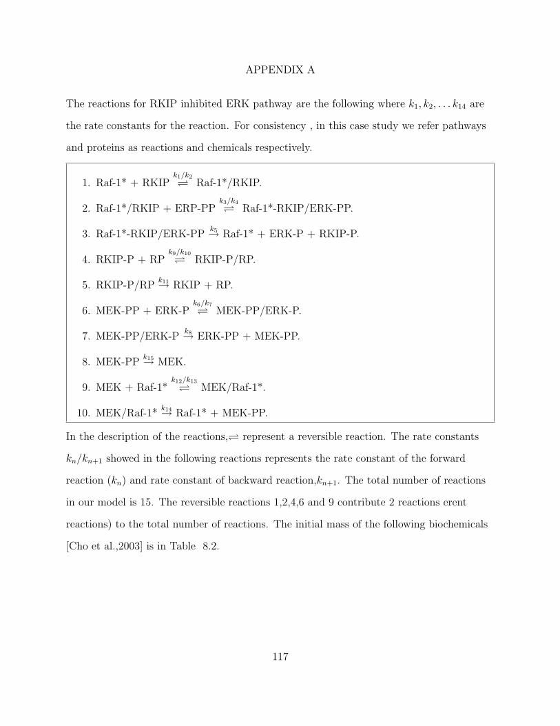
APPENDIX A

The reactions for RKIP inhibited ERK pathway are the following where k1, k2, . . . k14 are

the rate constants for the reaction. For consistency , in this case study we refer pathways

and proteins as reactions and chemicals respectively.

1. Raf-1* + RKIPk1/k2 Raf-1*/RKIP.

2. Raf-1*/RKIP + ERP-PPk3/k4 Raf-1*-RKIP/ERK-PP.

3. Raf-1*-RKIP/ERK-PPk5→ Raf-1* + ERK-P + RKIP-P.

4. RKIP-P + RPk9/k10 RKIP-P/RP.

5. RKIP-P/RPk11→ RKIP + RP.

6. MEK-PP + ERK-Pk6/k7 MEK-PP/ERK-P.

7. MEK-PP/ERK-Pk8→ ERK-PP + MEK-PP.

8. MEK-PPk15→ MEK.

9. MEK + Raf-1*k12/k13 MEK/Raf-1*.

10. MEK/Raf-1*k14→ Raf-1* + MEK-PP.

In the description of the reactions, represent a reversible reaction. The rate constants

kn/kn+1 showed in the following reactions represents the rate constant of the forward

reaction (kn) and rate constant of backward reaction,kn+1. The total number of reactions

in our model is 15. The reversible reactions 1,2,4,6 and 9 contribute 2 reactions erent

reactions) to the total number of reactions. The initial mass of the following biochemicals

[Cho et al.,2003] is in Table 8.2.

117

k1 k2 k3 k4 k5 k6 k7 k8

0.53 0.0072 0.625 0.00245 0.0315 0.8 0.0075 0.071k9 k10 k11 k12 k13 k14 k15

0.92 0.00122 0.87 0.05 0.03 0.06 0.02

Table 8.1: Rate of Reactions [Cho et al.,2003, Calder et al.,2010]

Biochemicals Raf-1* RKIP MEK-PP ERK-PP RPMass in intervals(in µM) [65-70] [0-1] [62-70] [172-182] [160-165]

Table 8.2: Initial Mass of the biochemicals in ERK pathway

118

domingo/teaching/ciic8996/Formal Analysis of... · Formal Analysis of Automated Model Abstractions...

Documents

Transcript of domingo/teaching/ciic8996/Formal Analysis of... · Formal Analysis of Automated Model Abstractions...