Dollarization and Financial Integration

Cristina Arellano∗

University of Minnesota

Jonathan Heathcote†

Georgetown University and CEPR

November 16, 2005

Abstract

This paper builds a simple theoretical model designed to study the effects of dollarization on

financial conditions. We compare allocations under two regimes: a flexible exchange rate regime

and a dollarized regime. Under flexibility, each period a benevolent government decides how

much to borrow or lend on an international bond market and the devaluation rate. Under dol-

larization the government decides only its debt policy. In equilibrium, international borrowing

is limited endogenously such that the government always chooses to repay when the penalty for

default is permanent future exclusion from financial markets. Dollarization implies the loss of

the devaluation rate as a policy instrument, but may still be optimal. The reason is that floating

defaulters can use the devaluation rate as a substitute for debt in responding to country-specific

shocks while dollarized economies in default find themselves in a more uncomfortable situation.

Thus dollarization reduces a government’s incentives to default, and thereby increases a coun-

try’s ability to borrow in equilibrium. We quantify these gains by calibrating the model to three

countries for which dollarization has been implemented or considered: Mexico, El Salvador and

Ecuador, and find that El Salvador features the greatest gains from dollarization.

∗arellano@econ.umn.edu†jhh9@georgetown.edu

1 Introduction

The recurrence of currency and financial crises in emerging markets has generated an intense

debate on the appropriate exchange rate regime. Dollarization has attracted special attention,

in part because of the recent official dollarization of Ecuador and El Salvador.1

The most important difference between dollarizing and simply pegging the exchange rate

is that dollarizing represents more permanent restrictions on domestic monetary policy. Thus

thinking about dollarization leads one to thinking about what a government might have to gain

by tying its hands more tightly with regards to monetary policy, which in turn leads to the issue

of credibility. In discussing papers in a conference volume on the topic of dollarization, Sargent

(2001) writes

“In their papers and verbal discussions, proponents of dollarization often appealed

to commitment and information problems that somehow render dollarization more

credible and more likely to produce good outcomes. Those proponents presented no

models of how dollarization was connected with credibility. We need some models."

In this paper we explore one avenue via which dollarization may increase credibility. In par-

ticular, we explore a model in which dollarization enhances a borrowing government’s credibility

in international financial markets, and thereby increases international financial integration.

The basic idea is as follows. Emerging-markets economies are typically subject to big shocks,

large fractions of government revenue are linked to volatile commodity prices, and raising tax

rates often increases evasion and substitution towards the informal sector. Thus traditional

sources of government revenue are often volatile and difficult to adjust. In this context seignior-

age is a valuable fiscal instrument, since extra money can rapidly be printed as required.

At the same time, emerging-markets economies also issue debt to smooth fluctuations and to

ease temporary liquidity problems. Dollarization can help strengthen fragile sovereign debt mar-

kets by increasing borrowers’ incentives to repay loans. The reason is that debt and seigniorage

are partial substitutes as revenue sources, so that an economy with an independent monetary

policy is prone to default, even if this means future exclusion from credit markets. Dollarization

makes the ability to access international debt markets more valuable, reducing the likelihood of

default and thereby loosening credit constraints.

We study a small open endowment economy populated by consumers, firms and a govern-

ment. Consumers work for firms, and each period they produce a stochastic quantity of goods

that can be used for private or public consumption. Firms sell these goods in exchange for cash.

Once the goods market has closed, firms pay their workers. Thus the cash that consumers spend

on goods in the current period must be carried over from the previous period. The government

1Dollarization in the broad sense of unilaterally adopting a stronger foreign currency such as the U.S. Dollar,Euro, or Yen.

2

is not subject to a cash-in-advance constraint: as long it has control over monetary policy it can

print new money after observing firm output and spend it immediately to purchase goods that

will be provided publicly. The government is benevolent and rational, and seeks to maximize

the utility of a representative consumer. In addition to revenue from seigniorage, the govern-

ment also trades one period bonds in international financial markets at a constant real interest

rate. However, the government cannot commit to repay international debts; contracts must be

self-enforcing. Thus foreign creditors set borrowing limits such that the government always has

the incentive to honor its obligations, where the penalty in case of default is permanent financial

autarky.

In addition to output shocks, the economy is also subject to taste shocks in the form of

changes to the relative taste for publicly versus privately-provided consumption. Taking as

given the process for shocks, the government chooses one of two possible exchange rate regimes:

flexibility or dollarization. Under flexibility, the government sets the money growth rate and

implicitly the inflation and devaluation rate period-by-period. Under dollarization, the inflation

rate is constant and equal to zero, and the government receives no revenue from seigniorage.

Thus once dollarized the government’s only policy instrument is its international debt position.

The dollarization decision is assumed to be irreversible 2 For simplicity, the government does

all the international borrowing and lending in the economy.

To assess quantitatively the effect that dollarization has on financial integration, we calibrate

our model to three countries: Mexico, El Salvador and Ecuador so that the flexible exchange rate

economy replicates some key features the economies. We calibrate to these countries because

they have been frequently been discussed as a candidates for dollarization with El Salvador and

Ecuador having in fact implemented dollarization. We find that large taste shocks are required

to account for the fact that government expenditure (and government consumption) is much

more volatile than GDP. The model does a good job in terms of replicating some key empirical

correlations in all three countries, such as the countercyclicality of inflation and the positive

correlation between government consumption and inflation.

By comparing the flexible regime to the dollarized regime, we find that the dollarized econ-

omy exhibits looser borrowing constraints and less frequent debt crises, identified as periods

in which the borrowing constraint is binding. We find that El Salvador features the greatest

gains from dollarization in terms of better financial conditions. In our model dollarization has

the greatest impact on financial integration when the economy’s fluctuations come in large part

by varying government needs as opposed to varying output. The reason is that debt policy is

a good substitute for the inflation policy when inflation is being used to finance government

shocks and thus dollarization has the least costs in this case. We find evidence that El Salvador

2In reality, it is presumably possible, though costly to de-dollarize a dollarized economy. However, the keydifference between dollarization and a fixed exchange rate regime is precisely that under dollarization it is morecostly to allow the exchange rate to float.

3

faces larger fluctuations coming from government shocks and thus dollarization has its greatest

net benefit.

>In order to address welfare issues, we then move to consider the version of the model in

which the economy starts out under a floating regime, and each period the government decides

whether or not to dollarize. We find that dollarization is the optimal regime choice when taste

shocks are relatively large to productivity shocks, and when the government’s international debt

becomes sufficiently large.

1.1 Historical experience

Our model predicts that dollarizing economies should exhibit greater international borrowing

ability - which may by manifested either as an increase in international borrowing or as a decline

in risk-premia - in addition to declines in the level and volatility of inflation. There is not too

much direct historical evidence which can be used to test the model, but the experience of

the small number of countries that have dollarized appears to be broadly consistent with the

predictions of our theory.

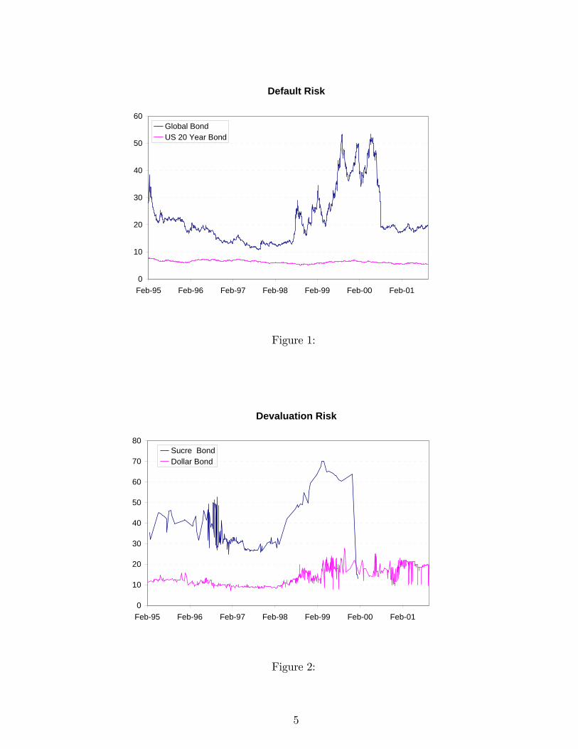
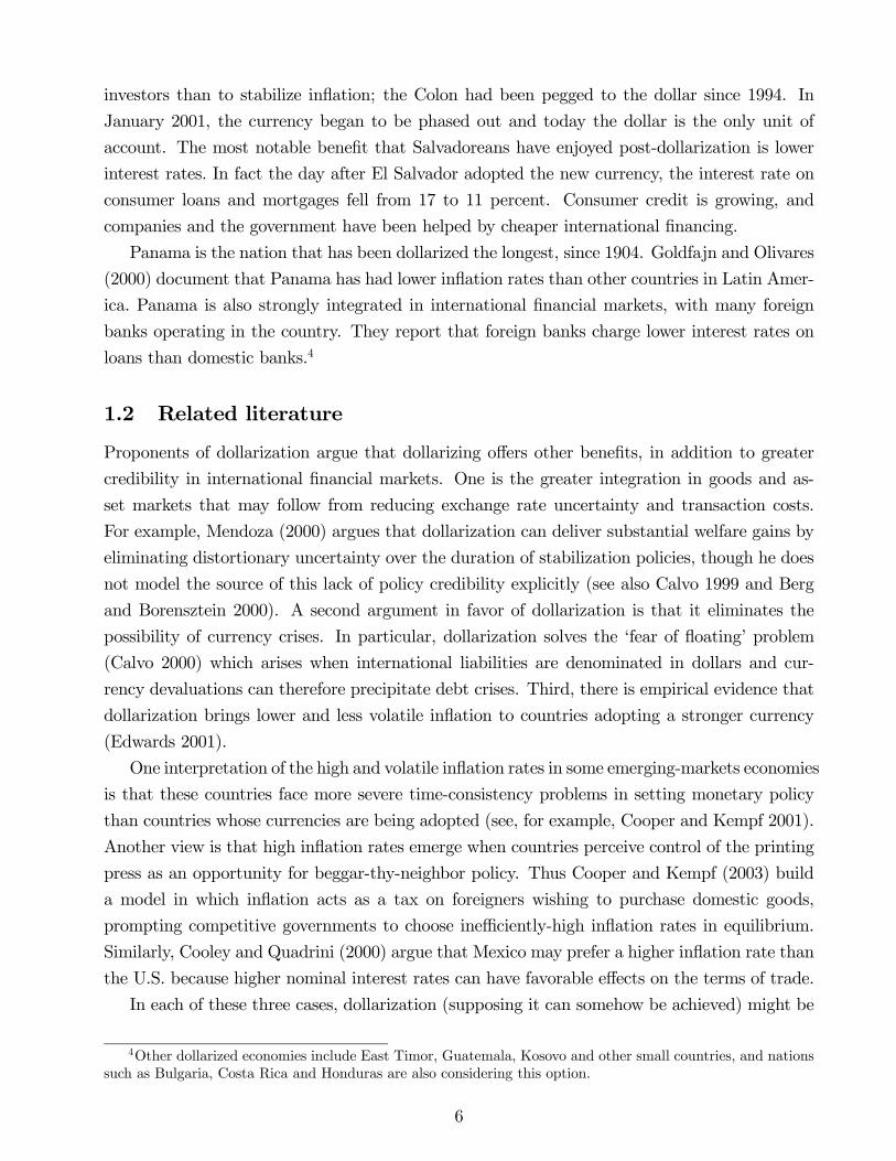
Ecuador dollarized in 2000 in the midst of a severe economic crisis with a collapsing banking

system, a sliding local currency, and after defaulting on its Brady bonds late in 1999. The

regime was implemented in an attempt to reduce inflation, bring stability to the economy, and

gain credibility with international investors. Since dollarization, Ecuador’s inflation has been

significantly reduced to single digits and the country has been able to renegotiate its debts at

somewhat lower interest rates.

Figure 1 shows the yields on Ecuadorian government bonds denominated in dollars that

are traded internationally , (JP Morgan Emerging Market Bond Index for Ecuador), together

with the yield on US 20 year government bonds. The difference in these two yields is a

common measure of default risk. The figure shows that default risk increased significantly in

1998 precluding the 1999 crisis and default. In July 2000 the yields came down again after

Ecuador dollarized and renegotiated its debt. Figure 2 shows the yields on domestic Ecuadorian

government bonds denominated in dollars and in sucres (Ecuador’s domestic currency before

dollarization). The difference between these two yields is a broad measure of devaluation

risk because both types of bonds are traded locally, have similar terms and conditions, and

the difference is the currency denomination.3 The figure shows that devaluation risk increased

dramatically in 1998, and it collapsed to zero when the economy dollarized. A key feature from

these figures is that devaluation risk and default risk move together as periods with high default

probabilities are associated with expectations of devaluations.

El Salvador implemented its dollarization plan in 2001 more in an effort to attract foreign

3Sucre and Dollar Bond yields are on 4 to10 year maturity bonds. In Ecuador, the domestic market forgovernment bonds is thin, and due to the lack of data we grouped the longer maturity bonds available to reportthe time series of yields.

4

Default Risk

0

10

20

30

40

50

60

Feb-95 Feb-96 Feb-97 Feb-98 Feb-99 Feb-00 Feb-01

Global BondUS 20 Year Bond

Figure 1:

Devaluation Risk

0

10

20

30

40

50

60

70

80

Feb-95 Feb-96 Feb-97 Feb-98 Feb-99 Feb-00 Feb-01

Sucre BondDollar Bond

Figure 2:

5

investors than to stabilize inflation; the Colon had been pegged to the dollar since 1994. In

January 2001, the currency began to be phased out and today the dollar is the only unit of

account. The most notable benefit that Salvadoreans have enjoyed post-dollarization is lower

interest rates. In fact the day after El Salvador adopted the new currency, the interest rate on

consumer loans and mortgages fell from 17 to 11 percent. Consumer credit is growing, and

companies and the government have been helped by cheaper international financing.

Panama is the nation that has been dollarized the longest, since 1904. Goldfajn and Olivares

(2000) document that Panama has had lower inflation rates than other countries in Latin Amer-

ica. Panama is also strongly integrated in international financial markets, with many foreign

banks operating in the country. They report that foreign banks charge lower interest rates on

loans than domestic banks.4

1.2 Related literature

Proponents of dollarization argue that dollarizing offers other benefits, in addition to greater

credibility in international financial markets. One is the greater integration in goods and as-

set markets that may follow from reducing exchange rate uncertainty and transaction costs.

For example, Mendoza (2000) argues that dollarization can deliver substantial welfare gains by

eliminating distortionary uncertainty over the duration of stabilization policies, though he does

not model the source of this lack of policy credibility explicitly (see also Calvo 1999 and Berg

and Borensztein 2000). A second argument in favor of dollarization is that it eliminates the

possibility of currency crises. In particular, dollarization solves the ‘fear of floating’ problem

(Calvo 2000) which arises when international liabilities are denominated in dollars and cur-

rency devaluations can therefore precipitate debt crises. Third, there is empirical evidence that

dollarization brings lower and less volatile inflation to countries adopting a stronger currency

(Edwards 2001).

One interpretation of the high and volatile inflation rates in some emerging-markets economies

is that these countries face more severe time-consistency problems in setting monetary policy

than countries whose currencies are being adopted (see, for example, Cooper and Kempf 2001).

Another view is that high inflation rates emerge when countries perceive control of the printing

press as an opportunity for beggar-thy-neighbor policy. Thus Cooper and Kempf (2003) build

a model in which inflation acts as a tax on foreigners wishing to purchase domestic goods,

prompting competitive governments to choose inefficiently-high inflation rates in equilibrium.

Similarly, Cooley and Quadrini (2000) argue that Mexico may prefer a higher inflation rate than

the U.S. because higher nominal interest rates can have favorable effects on the terms of trade.

In each of these three cases, dollarization (supposing it can somehow be achieved) might be

4Other dollarized economies include East Timor, Guatemala, Kosovo and other small countries, and nationssuch as Bulgaria, Costa Rica and Honduras are also considering this option.

6

viewed as increasing monetary policy credibility, in the sense of lowering the equilibrium inflation

rate. In this paper we pursue a different explanation for inflation dynamics in emerging-markets

economies: episodes of high and volatile inflation simply reflect periods during which less dis-

torting sources of revenue are not available. Thus in our model, policy is always time-consistent

and the devaluation rate does not have any beggar-thy-neighbor effects, but dollarizing still

reduces the mean and the variance of the inflation rate and the devaluation rate.

Among the costs of dollarization that are often cited are the loss of seigniorage revenues and

the inability to respond to external shocks with monetary policy (see, for example, Schmitt-

Grohe and Uribe 2001). For developed economies, the advantage of monetary independence is

usually expressed in terms of the ability to adjust the short-run real interest rate or the real

exchange rate in response to country-specific shocks. For emerging-markets economies, there is

often a simpler reason to want to retain the ability to print one’s own currency - seigniorage can

be an important and flexible source of government revenue. We will document the importance

of seigniorage revenue for Mexico and other emerging-markets economies later in the paper.

Canzoneri and Rogers (1990) explore the importance of seigniorage in the European Union, and

find that the optimal inflation rate is country-specific depends on differences in the efficiency of

tax collection systems across countries.

Sims (2002) argues that dollarization is costly because it prevents the economy from issuing

(state-contingent) nominal debt, without affecting dollar interest rates. However, governments

in emerging markets are largely unable to issue external debt in their own currency, no matter

what exchange rate regime they have, so it is not clear that this constitutes a strong argument

against dollarization in practice.

2 Model

The economy is populated by a large number of identical, infinitely-lived consumers, a repre-

sentative firm, and a government. In each period t = 0, 1, ... the economy experiences one of

finitely-many events st. We denote by st = (s0, ...st) the history of events up to and including

period t. The probability, as of date 0, of a particular history st is φ(st). The initial realization

s0 is given.

2.1 Firms

The representative firm in the economy produces a stochastic amount of output y(st) at date t

given history st. This good can be converted into a private consumption good c(st) or a public

consumption good, g(st). Output is produced at the start of the period, and then allocated

between consumers and the government in a cash market in the middle of the period. At the

end of the period, firms pay their workers (consumers) nominal wages w(st).

7

2.2 Consumers

Consumers are infinitely-lived, discount at rate β, and derive utility from both privately and

publicly provided consumption goods. Expected lifetime utility is given by

∞Xt=0

βtXst

φ(st)u(c(st), g(st), λ(st)) (1)

Period utility takes the following separable form:

u(c(st), g(st), λ(st)) =1

1− γ

£λ(st)c(st)1−γ + (1− λ(st))g(st)1−γ

¤0 < λ(st) < 1,

where λ(st) is a stochastic taste shock. We view λ(st) as capturing changes through time in

household preferences for public versus private goods, or changes in the taste for the allocation

mechanism (government provision versus market provision). One possible manifestation of these

changes in taste would be electoral cycles in which populist free-spending governments and more

fiscally conservative market-oriented governments take turns in power. We will assume that

st = (yt, λt) evolves according to a first-order Markov process.

The representative consumer enters the period with money savings from the previous period

ns(st−1) and wages from the previous period w(st−1). He observes the endowment shock y(st),

the taste shock λ(st), and the price level P (st). He then decides how much of his money to

spend, subject to the cash-in-advance constraint and the budget constraint:

P (st)c(st) ≤ ns(st−1) + w(st−1) ≡ n(st−1) (2)

ns(st) = n(st−1)− P (st)c(st) (3)

where n(st−1) denotes total nominal balances carried into period t. Note that these two con-

straints jointly imply ns(st) ≥ 0. Let

np(st) ≡ n(st−1)− ns(st)

denote money used for purchases by the household at date t.

2.3 Household Problem

The household problem is to choose the sequence of money savings ns(st) and consumptions

c(st) to maximize expected lifetime utility (eq 1) subject to the cash-in-advance constraint (eq.

2), the budget constraint (eq. 3) and a non-negativity constraint on consumption, c(st) ≥ 0,taking as a given a complete set of date and state contingent endowments y(st), taste shocks

8

λ(st), wages w(st), prices P (st), probabilities φ(st), and initial money holdings n(s−1) :

The inter-temporal first order condition for the household’s problem is

φ(st)u1(c(st), g(st), λ(st)) ≥ β

Pst+1

∙φ(st, st+1)

µu1(c(s

t, st+1), g(st, st+1), λ(s

t, st+1))

π(st, st+1)

¶¸(4)

with equality if ns(st) > 0

where π(st, st+1) denotes the gross inflation rate when next period’s state is st+1.

The transversality condition is

limst→s∞

βtPstφ(st)u1(c(s

t), g(st), λ(st))ns(st)

P (st)= 0. (5)

2.4 Government

The government is the only actor in the economy with access to a competitive international

bond market.5 In the bond market the government can borrow and lend one-period real bonds.

We assume that international lenders can decide whether to lend, how much to lend, and at

what price to lend. However they cannot make the price of loans contingent on the borrowing

government’s current net bond position, on net bond purchases, or on the shocks that will hit the

economy in the next period. Thus asset markets are far from complete. However, the assumed

market structure seems appropriate for emerging-markets economies, for whom international

borrowing must typically be repaid at non-contingent dates in non-contingent numbers of U.S.

dollars.

International debt contracts are not externally enforceable. We assume that lenders can

commit to honor their debt contracts, but the domestic government cannot commit not to

default on its debt obligations if it is an international net debtor. If it defaults, creditors are

assumed to credibly punish the government by permanently excluding it from the bond market:

a government that has defaulted in the past can neither buy nor sell bonds.

International lenders in the bond market can earn a safe real return r on the world mar-

ket. Given the assumptions that bond prices must be non-contingent and that the market for

international loans is competitive, all lenders sell bonds at the same price 1/(1 + r). The only

way that lenders can assure repayment is by rationing credit.6 Thus lenders impose endogenous

borrowing constraints on the government such that no borrowing occurs beyond the point at

5In reality, non-government international trade in financial assets is growing, but it is still the case that mostexternal debt in countries where dollarization is considered a possibility represents government borrowing. Forexample, as of March 2003, Argentina government debt accounts for 67% of the total stock of foreign debt; inMexico, it accounts for 56% and in Ecuador it accounts for 73%.

6One could imagine an alternative market structure in which lenders offer a menu of contracts, each of whichspecifies a loan amount and an interest rate. Contracts for greater loan amounts would then be associated withhigher interest rates to compensate for greater risk of default. In equilibrium the unconditional expected returnto the lender would be equalized across contracts. This market structure is adopted in Arellano, 2003.

9

which the probability of default in the subsequent period is positive.

2.5 Government Problem when Floating

At time zero, the government in the flexible regime decides on a policy Λ = g(st), B(st), μ(st)which defines government consumption, asset holdings B(st), and the gross money growth rate

μ(st) for all t and for all st given some initial assets B−1.

The government is not subject to a cash-in-advance constraint. Thus it can print new money

D(st) within the period after observing y(st) and λ(st) and use this money immediately to help

finance public consumption, g(st). LetM(st) denote the aggregate stock of money in circulation

at the end of period t. Thus the money growth rate μ(st) is equal to

μ(st) =M(st)

M(st−1)=

M(st−1) +D(st)

M(st−1).

In addition to seigniorage and revenue from international borrowing, the government can

also seize a constant fraction of the endowment τ directly. This can be interpreted as a constant

tax on private-sector output, or as the government producing fraction τ of output. Thus the

government nominal budget constraint, prior to default, is given by:

P (st)g(st) = τP (st)y(st) +D(st)− P (st)B(st) + (1 + r)P (st)B(st−1) (6)

where B(st) are real riskless foreign assets purchased at st

In addition, the state-contingent borrowing constraint requires bonds purchased to exceed

some (typically negative) state-contingent limit:

B(st) ≥ B(st) (7)

The government is allowed to default at any date. If the government chooses to default at

st, for all histories sr consistent with st the government budget constraint becomes

P (st)g(st) = τP (st)y(st) +D(st). (8)

However, as noted above the lenders will not lend beyond the point at which the default

probability becomes positive. We assume that the constraints B(st) are tight enough to deter

the government from ever defaulting in equilibrium, but ”not too tight”. They are not too tight

in the sense that if the history is st and the start-of-period assets are B(st), the government

is exactly indifferent between repaying and defaulting. We will return to the not-too-tight

condition when we define an equilibrium.

10

2.6 Government Problem when Dollarized

The problem for the government in a dollarized economy differs from the one described above

in two respects. First, the money growth rate is not a domestic policy instrument. We assume

that in the dollarized economy, a foreign government (the United States) conducts monetary

policy to target some path for the foreign inflation rate. Assuming the law of one price holds,

the domestic price and inflation rate will equal their foreign counterparts at every date. We

assume that the foreign government retains any seigniorage it collects from supplying cash to

the domestic economy. Since printing new cash is not a source of revenue for the domestic

government, the term D(st) drops out of the government budget constraints pre and post

default, eqs. 6 and 8. When we compare the flexible and dollarized economies we will assume

that the foreign government targets a constant inflation rate equal to zero.

The second difference is that the maximum amount of borrowing allowed at a point in time,

B(st), will differ across the flexible and dollarized regimes. This is because default incentives will

vary with the exchange rate regime. In particular, if debt and seigniorage are good substitutes

for financing temporary spending needs, then borrowing constraints will likely be looser in

the dollarized economy. The reason is simply that the punishment for default (loss of the

debt instrument) is painful in the dollarized economy when monetary policy cannot be used to

substitute for debt, but less painful in the flexible regime, where post-default seigniorage can

be used in place of debt in periods when the government needs revenue.

2.7 Some Equilibrium Relationships

The relationships described below apply to both the flexible and dollarized economies. The

difference between the two regimes is that under flexibility new money in local circulation

D(st) is controlled by the domestic government and the associated seigniorage appears in the

domestic government budget constraint. In the dollarized economy, D(st) is controlled by the

foreign government, and associated seigniorage does not appear in the domestic government

budget constraint.

At the end of the period, firms pay as wages all the cash they hold. Thus

w(st) = P (st)(1− τ)y(st)

The market clearing condition for the cash goods market is

P (st)(1− τ)y(st) = np(st) +D(st) (9)

If D(st) is negative, the interpretation under flexibility is that the government is borrowing

goods abroad, selling them on the domestic market, and taking the money it receives in exchange

11

out of circulation. The interpretation under dollarization is that the foreign government is selling

goods in exchange for dollars.

In equilibrium, all the money in the economy at the end of the period (after firms have paid

wages) is held by households, so

M(st) =M(st−1) +D(st) = n(st)

Note that if households do no money saving (ns(st) = 0) we get the standard quantity

equation with velocity equal to one:

P (st)(1− τ)y(st) = n(st−1) +D(st) =M(st).

>From the goods market clearing condition, the price level is given by

P (st) =np(st) +D(st)

(1− τ)y(st)=

M(st)− ns(st)

(1− τ)y(st). (10)

Substituting P (st) into the consumer’s budget constraint, eq. 3, gives

ns(st) = n(st−1)−µnp(st) +D(st)

(1− τ)y(st)

¶c(st)

c(st) = (1− τ)y(st)

µnp(st)

np(st) +D(st)

¶= (1− τ)y(st)

µM(st−1)− ns(st)

M(st)− ns(st)

¶Note that if the household is not doing any money saving (ns(st) = 0), then c(st) = (1 −

τ)y(st)/μ(st).

By printing money, the government (domestic or foreign) controls:

bμ(st) ≡ M(st)− ns(st)

M(st−1)− ns(st)(11)

where bμ(st) is the effective gross tax rate on consumption.The inflation rate is given by

π(st+1) =P (st+1)

P (st)=

µM(st+1)− ns(st+1)

M(st)− ns(st)

¶y(st)

y(st+1)=bμ(st+1)bμ(st) np(st+1)

np(st)

y(st)

y(st+1)(12)

Thus inflation is related to the growth rates of the effective consumption tax rate, the growth

rate of cash used to purchase goods, and the growth rate of output.

At the end of period t there are some nominal dollars in the hands of households, M(st).

It is clear, however, that the dollar face value of this money is not going to be allocative. In

12

particular, let x(st) denote the fraction of cash on hand that agents save at st :

x(st) =ns(st)

n(st−1)

We can now express all real variables in terms of the sequences y(st), λ(st), B(st), μ(st) and

x(st), with no reference to nominal variables M(st), P (st) or D(st).

In particular, from 12 the real return to money saving is given by

π(st+1) =P (st+1)

P (st)=

µμ(st+1)− x(st+1)

μ(st)− x(st)

¶μ(st)

y(st)

y(st+1)(13)

Note that if the money savings rate x(st) = 0 then inflation does not depend on the current

money growth rate μ(st). If x(st) > 0 then increasing μ(st) (while holding constant future

money growth rates) will have a weaker impact on inflation, since households will respond to

faster money growth by reducing savings, driving up the price level at date t (see eq. 10) and

thereby reducing inflation between t and t+ 1.

>From 11 the effective gross tax rate on consumption is

bμ(st) = μ(st)− x(st)

1− x(st)

>From the household’s budget constraint 3 and the goods market clearing condition 9 we

can express consumption, c(st), real balances and real money savings as

c(st) =

µ1− x(st)

μ(st)− x(st)

¶(1− τ)y(st) (14)

M(st)

P (st)=

µμ(st)

μ(st)− x(st)

¶(1− τ)y(st) (15)

ns(st)

P (st)=

µx(st)

μ(st)− x(st)

¶(1− τ)y(st) (16)

Note that the money growth rate has a direct effect on consumption and an indirect effect

via x(st). The direct effect is that faster money growth reduces purchasing power and reduces

consumption. The indirect effect is that if x(st) is positive, then agents will partially compensate

by reducing savings.7

dc

dx= 1− μ

The real value of seigniorage (received by the domestic government under flexibility, and by

7Note that faster money growth in period t (higher μ(st)) does not reduce the savings rate in period t becauseagents want to avoid seeing their money devalued; their money will be devalued whether they spend it or saveit.

13

the foreign under dollarization) is:

D(st)

P (st)=

M(st)−M(st−1)

P (st)=

µμ(st)− 1

μ(st)− x(st)

¶(1− τ)y(st) (17)

Note that x(st) ∈ [0, 1] .Setting μ(st) = 1 implies zero seigniorage. As μ(st) → ∞, D(st)P (st)

→(1 − τ)y(st) and thus c(st) → 0. Note that for μ(st) ≥ 1 seigniorage is (weakly) positive. Forμ(st) < 1, seigniorage is negative.

Note that consumption plus seigniorage is equal to the fraction of domestic output that is

not taxed directly:

c(st) +D(st)

P (st)= (1− τ)y(st)

Substituting this equation into the government budget constraint for the flexible economy,

we see that real domestic absorption is independent of the money growth rate under flexibility:

c(st) + g(st) = y(st)−B(st) + (1 + r)B(st−1) (18)

Note that there is no analogue to eq. 18 in the dollarized economy.

3 Definition of Equilibrium

We first define equilibrium for two economies that are not of direct interest, but that are useful

for defining borrowing constraints that are not too tight. The first economy is one in which:

(i) the borrowing constraints B(st) are exogenous, and (ii) the government must respect theconstraints and is not allowed to default. The second economy is one that has defaulted in

the past and has no access to the international debt market. The third economy, which is the

economy of interest, features borrowing constraints that are not too tight. In this economy

default is permitted but never observed in equilibrium.

Definition 1 Equilibrium with exogenous borrowing constraints. Consider a set of constraintseB =n eB(st)o ∀t ≥ 0 and for all st. A competitive continuation equilibrium given history sr

and initial assets Br−1 is a policy Λr and an associated allocation rule mapping policies into

private savings choices xr(Λr) such that for all t ≥ r and for all st consistent with sr : (i)

the household’s intertemporal first order condition 4 and transversality condition 5 are satisfied

when consumption is given by 14, inflation is given by 13, and real money savings are given

by 16, (ii) the policy is feasible: eqs. 6 and 7 are satisfied given initial assets Br−1 and the

constraints eB, and c(st), g(st) ≥ 0 when seigniorage D(st)/P (st) is given by 17 in the flexibleeconomy, and is equal to zero in the dollarized economy.

Definition 2 Post-default equilibrium. A post default equilibrium is defined in exactly the same

14

way, except that feasibility for the government requires B(st) = 0 for all t, st. Thus eqs. 6 and

7 are replaced by 8

Definition 3 Ramsey problem. The time zero Ramsey problem is to choose a policy Λ0 that

maximizes expected lifetime utility 1 when the allocation rule x0(Λ0) satisfies the conditions for

competitive equilibrium. The Ramsey equilibrium is the solution to the Ramsey problem.

Let W (Br−1, sr; eB) denote the value of Ramsey equilibrium with exogenous borrowing con-

straints eB, given assets Br−1 and history sr. Let V (sr) denote the value of the Ramsey post-

default equilibrium.

Definition 4 Borrowing constraints that are not too tight. A set of borrowing constraints B =B(st) for all t ≥ r, st such that for all st+1 in which φ(st, st+1) > 0

minst+1 st. φ(st,st+1)>0

W (B(st),¡st, st+1

¢;B)− V

¡st, st+1

¢= 0 (19)

Definition 5 Monetary equilibrium with competitive riskless lending. This is defined in exactlythe same way as the economy with exogenous borrowing constraints, except that (i) the borrowing

constraints are defined by the solution to eq. 19 (i.e. they are not too tight), and (ii) at each t

and st the government has the option of defaulting, in which case from t onwards eqs. 6 and 7

are replaced by the constraint 8.

Note that for a given set of constraints B, the value W (a, st;B) is strictly increasing in a

for any st, while the value of default is independent of the quantity of debt defaulted on. It

follows immediately that if for any (st, st+1) the government weakly prefers not to default given

inherited assets B(st) the government will strictly prefer to repay for any a > B(st). Conversely,

if the government is indifferent about default for some st+1 given st, then if a < B(st) and st+1

is realized, the government will strictly prefer to default. Note that if all lenders but one were

in total willing to lend an amount strictly less than B(st) in st, then the last lender could make

a positive profit on a marginal additional loan by charging a real interest rate greater than r

and bearing no default risk (assuming the government is borrowing constrained at st). Thus

the only equilibrium in the lending market in which no excess profits remain is one in which

lenders are willing in aggregate to lend up to B(st) at the safe world interest rate r.

3.1 Ramsey Equilibria

We now describe how we solve for the Ramsey equilibrium in our economies. Solving the Ramsey

problem in the dollarized economy is simpler, because monetary policy in this case is exogenous,

and the planner only needs to decide on the optimal debt policy.

15

3.1.1 Dollarized Economy

The Ramsey equilibrium in the dollarized monetary economy with riskless lending can be charac-

terized by solving the following planner’s problem. Consider a planner who maximizes expected

lifetime utility (eq. 1) subject to budget constraints

g(st) = τy(st)−B(st) + (1 + r)B(st−1) (20)

and a set of borrowing constraints of the form eq. 7.

Sufficient conditions for a solution to this problem are the optimality conditions for bonds:

φ(st)(1− λ(st))g(st)−γ ≥ β(1 + r)Pst+1

£φ(st, st+1)(1− λ(st+1))g(st+1)−γ

¤(21)

with equality if B(st) > B(st)

limst→s∞

βtPstφ(st)(1− λ(st))g(st)−γ

¡B(st)−B(st)

¢= 0. (22)

Note that in the dollarized economy, separability between private and public consumption

in preferences implies that consumers and the government end up solving completely separate

problems. Consumers use money savings to smooth the marginal utility of private consumption

through time, taking as given inflation rates. The government uses debt to smooth the marginal

utility of public consumption through time, taking as given the world interest rate and state-

contingent borrowing constraints.

3.1.2 Flexible Economy

Wewill show that the Ramsey equilibrium in the flexible monetary economy with riskless lending

can be characterized by solving the following planner’s problem.

Planner’s Problem Without Money Consider a planner who maximizes expected lifetime

utility (eq. 1) subject to a set of borrowing constraints of the form eq. 7 and an aggregate

resource constraint 18.

Sufficient conditions for a solution to this planner’s problem are the optimality conditions

for bonds (eqs. 21 and 22) described above and an intra-temporal first-order condition

λ(st)c(st)−γ = (1− λ(st))g(st)−γ (23)

which says that the planner wants to equate the marginal utilities of privately and publicly

provided goods at each date.

Combining 18 and 23 gives

c(st) =R(st)

(1 + κ)(24)

16

where

R(st) = y(st)−B(st) + (1 + r)B(st−1) (25)

κ(st) =

µλ(st)

(1− λ(st)

¶− 1γ

Thus

g(st) = κ(st)c(st) (26)

Note that because the marginal utilities of private and public consumption are equated state-

by-state, the inter-temporal first order condition 21 can be expressed in terms of c(st), g(st) or

total resources available for domestic consumption R(st). For example, in the case γ = 1, the

first order condition simplifies to

φ(st)

R(st)≥ β(1 + r)

Pst+1

∙φ(st, st+1)

R(st, st+1)

¸.

Thus in this case, the planner simply wants to smooth fluctuations in the endowment through

time, irrespective of the process for taste shocks: a floating, credit-worthy government will

typically issue when the endowment is relatively low, and repay when the endowment is high.

Decentralization Proposition Suppose the borrowing constraints faced by this planner

are "not too tight" in the same sense that we defined not-too-tight constraints in the flexible

monetary equilibrium with competitive riskless lending. Suppose γ = 1. Then the allocations

c(st), g(st) and B(st) that solve the planner’s problem without money also solve the Ramsey

problem in the monetary economy with riskless lending, and the values of the not-too-tight

borrowing constraints are also the same in both economies.

Note that the Ramsey planner in the monetary economy maximizes the same objective as

in the planner’s problem above, faces the same aggregate resource constraint period-by-period

(the consumers and government budget constraints, eqs. 14 and 6 imply eq. 18), and will have

the same optimality conditions for debt. Thus it remains to show that the government in the

monetary economy, in which control of the money growth rate is the only way to reallocate

resources between the public and private sectors, can achieve the same allocations as a planner

who can effectively use lump-sum taxes and transfers to redistribute freely period by period. In

particular, we need to show that there exist sequences for money growth rates μ(st), inflation

rates π(st+1) and savings rates x(st) such that:

(i) The consumer’s budget constraint is satisfied: given the target values for consumption

(eq. 24), μ(st) and x(st) satisfy the budget constraint (eq. 14). This implies that the savings

17

rate can be expressed as

x(st) =c(st)μ(st)− (1− τ)y(st)

c(st)− (1− τ)y(st)(27)

(ii) The government’s budget constraint is satisfied: given the target values for consumption

(eq. 24), μ(st) and x(st) satisfy the budget constraint (eq. 6).

(iii) The optimality conditions for money savings are satisfied: given the target values for

consumption, μ(st), π(st+1) and x(st) are such that if

φ(st)λ(st)c(st)−γ > βPst+1

∙φ(st, st+1)λ(s

t+1)c(st+1)−γ1

π(st+1)

¸(28)

where the inflation rate π(st+1) is given by

π(st+1) =¡μ(st+1)− x(st+1)

¢ y(st)

y(st+1)(29)

then today’s money growth rate is given by8

μ(st) =(1− τ)y(st)

c(st). (30)

Otherwise, if the strict inequality in 28 does not hold, money growth rates are defined by

the difference equation

φ(st)λ(st)c(st)−γ =Pst+1

∙φ(st, st+1)λ(s

t+1)c(st+1)−γ1

π(st+1)

¸(31)

and the transversality condition

limst→s∞

βtPstφ(st)λ(st)c(st)−γ

M(st)

P (st)= 0. (32)

where π(st+1) is given by 13, and real balances M(st)/P (st) are given by 15.

Proof of Decentralization Proposition First note that if savings rates are given by 27 then

the consumer’s budget constraint is satisfied, and since the aggregate resource and borrowing

constraints must be satisfied - they appear in the constraint set of the planner’s problem without

money - the government’s budget constraint is satisfied by Walras’ Law. Thus it only remains

to show that there exists a set of money growth rates μ(st) that can implement the target values

for c(st) while satisfying the optimality conditions for money savings.

Suppose that borrowing constraints are not too tight according to the planner’s problem, and

that the sequence for government debt solves the planner’s problem. We will show that for any

8Note that from 27 this implies that x(st) = 0.

18

possible monetary policy implemented after some date T, we can decentralize the target values

for c(st) and g(st) between periods 0 and T in a monetary equilibrium with riskless lending.

Total resources R(st) in the planner’s solution are given by eq. 25. A sufficient condition for

proving that the planner’s choices for c(st) and g(st) can be implemented is that the planner

can implement any value for c(st) ∈ (0, R(st)) for all st and for all t ≤ T. This amounts to

showing that the monetary authority effectively has access to a lump-sum tax instrument. To

verify that the condition is satisfied we need to understand the response of prices and quantities

to changes in the money growth rate.

Note first, that because this is an endowment economy, neither money growth nor inflation

have any distortionary effects on factor supplies. Suppose that from period T + 1 onwards,

the government will follow a particular policy defined by ΛT+1. The money growth rate at st,

μ(st), will affect c(st), x(st) and π(st+1). However it will not affect future savings rates and

consumption values, which will depend solely on ΛT+1. Past monetary policy does not restrict

the set of feasible allocations that can be achieved looking forward, because current and future

policy determine the real value of the dollars consumers carry into the period, which is what

matters for real allocations.9 Given arbitrary choices for T, sT and the tax rate τ we will show

first that the government can implement any value for c(sT ) ∈¡0, R(sT )

¢with an appropriate

choice for μ(sT ), and thus we can also implement the c(sT ) that solves the planner’s problem

without money Then we can work backwards to compute the value for μ(sT−1) that delivers

the appropriate c(sT−1), exploiting once again the fact that changes in μ(sT−1) do not impact

c(sT−1, sT ). In this fashion we can work backwards all the way to period 0, along the way

deriving sequences for μ(st), π(st+1) and x(st) that decentralize the planner’s solution.

We guess, and will verify, that given a particular monetary policy from tomorrow onwards,

there will be a critical money growth rate μ(st) such that for any μ(st) ≥ μ(st) the money

savings rate x(st) is constant and equal to zero, while for μ(st) < μ(st) the savings rate x(st) is

continuous and decreasing in μ(st), with the property that x(st)→ 0 as μ(st)→ μ(st).

If the target value for c(st) is less than or equal to

c(st) =(1− τ)y(st)

μ(st).

then it can be implemented with a money growth rate μ(st) defined by 30, where μ(st) ≥ μ(st)

and x(st) = 0. In this case, the lower is the target value for c(st) the higher is the required μ(st).

From 14, as μ(st)→∞, c(st)→ 0.

9The real purchasing power of consumers’ money balances entering the goods market at (st, st+1) is givenby

M(st)

P (st, st+1)=

µ1

μ(st, st+1)− x(st, st+1)

¶(1− τ)y(st, st+1)

and thus does not depend on μ(st) or x(st).

19

If the target value for c(st) is greater than c(st) then it will not be possible to implement in

a monetary economy without money savings. In this case, the required money growth rate will

be low or negative, savings x(st) will be positive, and the inter-temporal first order condition

for money saving will be an equality, eq. 31. Since c(st, st+1) > 0, μ(st, st+1) > x(st, st+1) for

all st+1, and using the expressions 14 and 13 for current consumption and the inflation rate

between t and t+ 1 the inter-temporal first order condition equation implicitly defines x(st) as

a continuous function of μ(st):

In particular, assuming γ = 1 and substituting in the expression for inflation from 13 the

inter-temporal first order condition may be written

λ(st)

c(st)= β

Pst+1

φ(st, st+1)

φ(st)

λ(st, st+1)

c(st, st+1;Λt+1)

(μ(st)− x(st)) y(st+1)

μ(st) (μ(st, st+1)− x(st, st+1;Λt+1)) y(st)(33)

Using 14 to express consumption as a function of x(st) and μ(st) gives

λ(st)μ(st)

(1− x(st)) (1− τ)= β

Pst+1

φ(st, st+1)

φ(st)

λ(st, st+1)

c(st, st+1;Λt+1)

y(st+1)

(μ(st, st+1)− x(st, st+1;Λt+1))(34)

It is immediate from this expression that the savings rate x(st) is everywhere decreasing

in μ(st).10 The critical money growth rate μ(st) is the value of μ(st) that solves 34 when

x(st) = 0. For μ(st) > μ(st) the inter-temporal first order condition will be a strict inequality

with x(st) = 0, confirming the guess that for money growth rates exceeding μ(st), household

maximization will imply no money saving.

The important point relating to our decentralization result is that when γ = 1 the savings

rate x(st) is uniformly decreasing in the money growth rate μ(st). The implication is that if

the government has infinite resources it can make seigniorage arbitrarily small and consumption

arbitrarily large by reducing μ(st) towards the point at which x(st) = μ(st) (see eq. 14). In

practice, of course the government does not have infinite resources, but it always has a least

R(st) − (1 − τ)y(st) resources from direct taxation and international borrowing. So it can

reduce the money growth rate to the point at which seigniorage is equal to, the negative of

this number, in which case c(st) = R(st). Thus we have shown that, for the case γ = 1, the

monetary authority can implement any value for c(st) ∈ (0, R(st)) with an appropriate choice10Here is some intuition for the response of x(st) to μ(st). Absent a change in the savings rate, a reduction in

the money growth rate μ(st) reduces the current price level P (st) and increases expected inflation π(st+1), whichtends to reduce savings. It also increases current consumption, and reduces the marginal utility of consumption,making consumers want to save more. With no change in the savings rate the second effect would dominate,leaving the marginal utility of consumption at st too low (see 34). Of course, in equilibrium prices and decisionsadjust so that the household’s inter-temporal first order condition is satisfied. When γ = 1 the equilibriumadjustment mechanism is that the expected inflation rate rises by more than under the no-savings-adjustmenthypothsis, and the savings rate rises. This increase in the savings rate is consistent with the inflation dynamic(see 13), and the reduced return to saving reduces the right hand side of the intertemporal first order condition.At the same time, a higher savings rate actually increases equilibrium consumption (see eq. 14), reducing theleft hand side of the first order condition, but for γ = 1 the first effect dominates.

20

for μ(st).

Since the monetary authority effectively has access to lump-sum taxes, it can and will set

μ(st) at each date to equalize the marginal utilities of private and public consumption state-by-

state, thereby achieving the same allocations as in the planner’s problem without money. Recall

that the planner uses debt to smooth fluctuations in the endowment over time. Thus monetary

policy will be used primarily to adjust the mix between private and public consumption in

response to taste shocks. When λ(st) is high, indicating a preference for private consumption,

the money growth rate μ(st) and thus seigniorage will be relatively low.

Decentralization When γ > 1 When γ > 1 the solution to the planner’s problem can still

be decentralized in a monetary equilibrium. However, there are multiple monetary equilibria,

and only one of them is constrained efficient.

[TO BE COMPLETED]

3.2 Three Questions

Here we briefly address three questions. First, for a given government policy in the monetary

economy, is there a unique equilibrium? Second, assuming the government can commit to

monetary policy under flexibility, is the welfare-maximizing monetary policy the same when

the government takes borrowing constraints as given versus when the government recognizes

that the position of constraints that are not-too-tight will depend in principle on the announced

policy? Third, is the policy that solves the Ramsey problem time consistent? We will argue

that for each of the questions, the answer is “yes”.

First, for a given monetary policy there is a unique monetary equilibrium when γ = 1.

This follows immediately from the fact that the savings rate x(st) is everywhere decreasing in

μ(st). In particular, for any policy ΛT+1 defining policy from period T + 1 and onwards, each

possible money growth rate μ(sT ) at sT implies a unique value for x(sT ) and thus for c(sT ) and

π(sT , st+1). A similar argument can be applied, recursively, at each date t ≤ T.When γ > 1, the

savings rate x(st) is not everywhere decreasing in μ(st). Furthermore, for a given ΛT+1, there

are typically ranges for the money growth rate within which one value for μ(sT ) supports more

than one combination of c(sT ), x(sT ) and π(sT , st+1) satisfying all the equilibrium conditions.

Thus for γ > 1 multiple equilibria can arise.

Regarding the second question, suppose that the government could credibly commit to a

future money growth rate policy prior to default, but cannot commit to repay foreign lending,

and cannot commit to monetary policy post-default. Is it possible that the government can

increase welfare beyond the value of the solution to the Ramsey problem, in which the govern-

ment takes the position of the borrowing constraints as given? The answer is no. The reason

is as follows. First, taking as given borrowing constraints that are not-too-tight, the solution

21

to the Ramsey problem described above maximizes value. Thus the only way a different policy

could potentially increase value would be if it implied looser borrowing constraints. However,

we can argue that not-too-tight constraints can only be tighter under alternative policies.

First, note that post default, the government will always set the money growth rate to

equalize the marginal utilities of private and public consumption. Thus changing monetary

policy prior to default cannot change the value of default. Second, prior to default, for any given

set of borrowing constraints, value inside the contract is maximized under the policy described

above, where monetary policy is used to equate the marginal utilities of private and public

consumption. Since value inside the contract could only be lower for any alternative monetary

policy, not-too-tight borrowing constraints could only be tighter under any alternative policy.

The third question was whether the policy that solves the Ramsey problem is time-consistent,

or whether the policy that maximizes expected value at time zero no longer looks optimal if

the government is allowed to re-optimize in some future date and state. The policy described

above is in fact time-consistent, because the optimal policy from st onwards is independent of

policy prior to date t. Potential deviations from the pre-announced policy would be to default

on outstanding debts, or to deviate from pre-announced debt or monetary policy. Default

will reduce welfare, given borrowing constraints that are not-too-tight. Deviating from pre-

announced debt policy will reduce welfare, since the pre-announced policy smooths government

consumption as effectively as possible. Deviating from pre-announced monetary policy will be

welfare-reducing, because such a change can only change the mix between private and public

consumption (in a welfare-reducing fashion) without changing the total resources R(st) in the

economy.

4 Quantitative Analysis

In this section we solve numerically the two monetary economies: one with a flexible exchange

rate regime, and the other one with a dollarized regime. The objective of the quantitative

analysis is to compare across regimes the degree of financial integration in terms of borrowing

constraints, probabilities of crisis, and debt policy. Our strategy is to calibrate the flexible

regime economy to countries in which dollarization has been discussed or implemented as their

exchange rate policy. We calibrate the model to three countries: El Salvador and Ecuador, that

dollarized in 2001 and 2000, and Mexico for which dollarization has been considered as possible

policy. With a given calibration for each country, we then solve the economies assuming a

dollarized regime and compare then in terms of business cycles and financial conditions.

22

4.1 Calibration

Data for real output, government consumption and household consumption in the three countries

is per capita annual data taken from the World Development Indicators for 1960-2002.11 To

study the dynamics of foreign public debt in our model we use the series for Government Foreign

Financing as a percentage of GDP taken from the International Financial Statistics for 1980-

2002. This series measures the change in net foreign assets held by the government. Inflation

is the percentage change in consumer prices. We log the series of output, private and public

consumption and filter all the data with a 15 year Band-Pass Filter.12 Figure 2 shows the raw

statistics and the filtered series of output for the three countries.

The stochastic structure for the shocks are calibrated for each country. We assume λ and y

follow are AR(1) jointly distributed log normal process, where their innovations are allowed to

be correlated. Allowing for correlation between shocks is important for giving the model enough

flexibility to match the business cycle statistics for the three countries. In particular we assume

the following stochastic structure:

log(yt) = ρ log(yt−1) + εyt

log(λt) = ρ log(λt−1) + ελt

E[εy] = E[ελ] = 0

E[εy0ελ] = Ω =

"σ2y σyλ

σyλ σ2λ

#The volatility and covariance of shocks are estimated jointly such that the model under the

flexible regime matches the volatility of government consumption, volatility of output, and the

correlation between government consumption and output in each of the countries. Thus σy,

σyλ, and σλ are calibrated country by country to match the data. We assume a common persis-

tence parameter ρ across shocks and across countries of 0.8, which is the average persistence of

output across the three countries. Shocks are discretized into a 25 state Markov process using

quadrature as in Tauchen and Hussey.

The annual interest rate r is set to 4% which is a standard value for real business cycle

models. We assume that utility is log separable with γ = 1. We choose the time preference

parameter β to match the volatility of public foreign assets in Mexico. The mean value for λ is

11The specific series we used from WDI are: General government final consumption expenditure, Householdfinal consumption expenditure, GDP, (denominated in real local domestic currency and divided by Population)and Inflation, consumer prices (annual %).

12We use a longer filter to keep some of the lower frequency movements that have been documented by Aguiarand Gopinath (2004) to be important for emerging countries.

23

set to 0.88 to match the mean government consumption to GDP ratio across the three countries.

We assume that default entails an extra cost of lowering the countries endowment by θ, which

we set to 1%. Table 1 summarizes the parameters values in the model.

Table 1.

Estimation of Parameters per Country

Target Statistics per Country Mexico El Salvador Ecuador

Volatility of output σy= 0.0257 σy= 0.0344 σy= 0.0281

Volatility of government consumption σλ= 0.0031 σλ= 0.0092 σλ= 0.0091

Correlation of government and output ρλy= −0.3226 ρλy= 0.4424 ρλy= −0.7430Common Parameters Across Countries

Persistence ρ = 0.8

Output costs post default θ = 1%

Mean government/output λ= 0.88

Public foreign assets volatility in Mexico β = 0.95808

4.2 Results

Table 2 presents business cycle statistics for the data in Mexico and for the model under the

flexible and dollarized regime. Consumption and output volatilities are similar in Mexico, with

consumption being slightly less volatile. Government expenditures are much more volatile than

output. Inflation in Mexico has been extremely volatile. In Mexico, the correlations among

private consumption, public consumption and output are positive. Inflation rates are weakly

negatively correlated with output, and positively correlated with government spending. In

Mexico, net public foreign assets are positively correlated with output and weakly positively

correlated with government consumption. Thus the government uses more foreign debt to

finance its budget in recessions.13

Table 2.

MEXICO Data Flexible Economy Dollar Economy

σx ρx,y ρx,g σx ρx,y ρx,g σx ρx,y ρx,g

Government 5.67 0.78 — 5.67 0.78 — 3.98 0.78 —

Consumption 3.84 0.94 0.67 3.40 0.93 0.71 3.94 1.0 0.91

Inflation 19.10 -0.09 0.24 2.71 -0.05 0.06 — — —

Public foreign assets 1.31 0.41 0.14 1.31 0.47 0.20 0.20 0.18 -0.23

Output 3.95 — 0.78 3.94 — 0.78 3.94 — 0.78

Borrowing constraint -24.81 -25.39

% in Crisis 39.02 25.63

13It has been documented that the trade balance is on the contrary countercyclical; however our emphasishere is on the public sector debt dynamics.

24

Table 3 shows business cycle statistics for the benchmark model with the calibration for

Mexico under flexible exchange rates and dollarization. Business cycle statistics are those of the

limiting distribution of assets. Our calibration suggests that productivity shocks are the most

important with the standard deviation of productivity shocks being 8 times larger than that of

taste shocks.

Standard deviations of output, government, and the public foreign assets and the correlation

of government and output were calibrated jointly by the choices for the standard deviations and

correlation of shocks and the time preference parameter. The flexible economy replicates some

other important features of the Mexican economy. The volatility of consumption is lower than

output volatility, as in the data. The model can also match the contemporaneous positive

correlation between government and private consumption, and the positive correlation between

government and output. In the model, the taste shock makes households value highly private

consumption, and simultaneously value public consumption less, which tends to make the cor-

relation negative. But productivity shocks imply a positive correlation, because when output is

high, the government optimally wants to increase both public and private consumption. Given

that productivity shocks are most important in Mexico, the model can generate the positive

correlations with private consumption.

The model matches the acliclycality of inflation and predicts a slightly positive correlation

between inflation and government as observed in Mexico. This is because in the flexible

economy, the government finances government consumption with the inflation tax revenue and

debt and thus when the economy has a large taste for government consumption inflation is

higher. However given that output shocks and government consumption taste are positively

correlated ( ρλy < 0), periods of high taste of government consumption are also periods of

high output. Thus inflation doesn’t need to be adjusted as heavily as to deliver the right level

of government consumption. However this same reason is also why the model misses the high

volatility of inflation observed in Mexico.

The model matches the procyclicality of public foreign assets. In the model with strong

productivity shocks, debt is used to smooth output fluctuations; the government runs down its

assets in periods of low output, and engages in precautionary savings in periods of relatively

high output.

Table 3 also presents statistics for the dollarized economy using the benchmark calibration.

The labor tax τ used equals 12.87, which is the optimal labor tax assuming that post default the

government adjusts one time the labor tax to the optimal post default level. In several respects,

the dollarized economy exhibits a slightly higher degree of international financial integration

than the flexible exchange rate economy. The dollarized economy can sustain more borrowing

in equilibrium as the endogenous borrowing constraint in the dollarized economy is looser than

in the flexible economy and the probability of being in crisis is smaller.14 The government of the

14We have assumed that all elements in the transition matrix are non-zero, such that the model generates a

25

dollarized economy has less incentives to default because debt is the only policy available for

smoothing government fluctuations, and thus the government’s credibility in financial markets is

increased. Figure 4 presents the distribution of assets in the limiting distribution for the flexible

and dollarized economies. Both economies have a distribution of assets that have a probability

mass at the constraint. The dollarized economy features a lower probability of being in a

financial crises: the probability mass at the respective constraint is 39% in the flexible economy

compared to 25% in the dollarized case. However the dollarized economy uses debt less strongly

as seen in the lower volatility of foreign assets and the smaller range for asset positions in the

limiting distribution.

Business cycle statistics in the dollarized economy, are qualitatively similar to those in the

flexible economy. Consumption volatility is exactly equal to output volatility, because in the

dollarized economy with constant taxes there is no way to affect the time path of private

consumption. Government consumption volatility is much smaller in the dollarized economy.

This suggests that for Mexico, debt in the dollarized regime is not as good of a substitute policy

for the inflation rate in the flexible regime. In our model dollarization changes the correlation

between foreign assets and government consumption by making it negative. In the dollarized

regime debt is used to finance volatile government consumption needs; the government borrows

when it faces a high taste for government consumption, and saves when it faces a low taste.

We next analyze the case of El Salvador. This country dollarized its economy in 2000

and here we use our model to analyze the effect of such policy on its international financial

integration.Table 3.

EL SALVADOR Data Flexible Economy Dollar Economy

σx ρx,y ρx,g σx ρx,y ρx,g σx ρx,y ρx,g

Government 9.73 -0.05 — 9.73 -0.04 — 8.27 -0.05

Consumption 7.58 0.90 -0.38 5.22 0.90 -0.22 5.27 1.0 0.12

Inflation 4.46 -0.29 0.19 3.96 -0.19 0.34 — — —

Public net foreign assets 0.48 0.03 -0.19 2.17 0.53 -0.18 1.19 0.45 -0.83

Output 5.27 — -0.05 5.27 — -0.04 5.27 — -0.04

Borrowing constraint -24.91 -25.56

% in Crisis 22.18 9.54

Business cycle statistics for El Salvador are quite different than for Mexico. Government

consumption is almost twice as volatile than output and private consumption is substantially

more volatile than output. Inflation in El Salvador features a negative correlation with out-

put and a positive correlation with government consumption. Public government consumption

present a negative correlation with both output and private consumption which is opposite from

the Mexican data. Lastly, public debt is acyclical and negatively correlated with government

single borrowing constraint for each regime.

26

consumption. Thus periods of high government expenditures needs are associated with periods

of larger debt levels.

Our calibration suggests that taste shocks are more important for El Salvador than for

Mexico, although productivity shocks are also very important. Productivity shocks are 3.7

times bigger than taste shocks for El Salvador calibration. In addition the calibration suggests

that the taste for government consumption is high in periods of low output. The sources of

shocks are important for the effect of dollarization on financial integration. As we show below

the increase in financial integration with dollarization is the largest when taste shocks are strong.

The flexible model calibrated to El Salvador matches many of the features of the data. The

model features the negative correlations of private and public consumption as in the data, the

countercyclicality of inflation, and the positive correlation of inflation and government con-

sumption. The model predicts that in El Salvador inflation is used heavily in periods of high

government consumption needs, not only due to a high taste for government consumption but

also because output is exactly lower in those periods. Thus this calibration generates a larger

volatility in inflation that is countercyclical.

In addition the model matches the positive correlation of public foreign assets and output

and the negative correlation of public foreign assets and government consumption. In the flexible

economy debt is used to smooth output fluctuations and taste shocks. The model generates a

negative correlation of foreign assets and government consumption because conditional on the

productivity shock, the government engages in more borrowing to finance the larger need for

government consumption. The model underestimates a bit the volatility of both inflation and

private consumption, but overall it provides a good fit to the Salvadorean data.

The table presents business cycle statistics for the dollarized regime, where we use a labor

tax τ of 0.1317 estimated in the same way as for Mexico. The dollarized economy calibrated to

El Salvador presents a higher degree of financial integration. The economy is able to borrow a

larger proportion of output, and the probability of being in crisis drops by half from 22% to 9%

of the time. In addition with this calibration, we find that debt in the dollarized regime is a

good substitute for the inflation policy in the flexible regime, as seen by the similar volatility of

government consumption across regimes. The reason why debt is a good substitute to inflation

for this calibration and not for the Mexican calibration is because a larger proportion of the

volatility of government consumption in El Salvador is coming from the volatility of taste shocks.

In the dollarized economy, borrowing is the largest when output is low, and when the taste for

government consumption is large and this states happen simultaneously for El Salvador. In

Mexico, taste shocks are small and are negatively correlated with output, and thus the economy

faces a trade-off such that debt cannot be used as effectively for the two purposes.

We now analyze the case of Ecuador which dollarized its economy in 2000. Business cycle

statistics in Ecuador have a similar flavor than those in Mexico in various aspects. Government

consumption is very strongly correlated with output and private consumption, and private

27

consumption is slightly less volatile than output; pointing to evidence of strong productivity

shocks. However in Ecuador government consumption is very volatile, more than 3 times as

volatile as output and inflation is countercyclical, pointing to evidence of taste shocks.

Our calibration suggests that taste shocks are quite strong in Ecuador but that they are

strongly positively correlated with productivity shocks. This suggests that government needs

increase when output increases but by much more. The reason for this relation is the oil

dependence that Ecuador has in terms of government consumption and output. Oil constitutes

a large source of government revenues and a large fraction of the economy as a whole and thus

both tend to move together.

The model under the flexible regime can match various aspects of the Ecuadorian economy,

but does a less good of a job than for the calibration of the other two countries. In particular it

predicts a lower volatility of private consumption, and a strong positive correlation of inflation

and output which is at odds with the data. The reason for the procyclicality of inflation is

that in booms government consumption needs are even higher than the increase in output, and

so inflation is high to finance it. Government consumption in the model is financed mainly

by inflation and not debt, because the government finds it better to save in those periods for

precautionary reasons given the high output.Table 4.

ECUADOR Data Flexible Economy Dollarized Economy

σx ρx,y ρx,g σx ρx,y ρx,g σx ρx,y ρx,g

Government 13.37 0.85 — 13.37 0.85 — 7.05 0.85 —

Consumption 4.29 0.90 0.81 2.97 0.84 0.61 4.32 1.00 0.83

Inflation 11.62 -0.21 -0.02 3.26 0.30 0.40 — — —

Public net foreign assets 0.75 0.10 0.06 1.54 0.49 0.33 0.50 -0.36 -0.82

Output 4.32 — 0.85 4.32 — 0.85 4.32 — 0.85

Borrowing Constraint -24.82 -25.36

% in Crisis 25.08 18.78

Our model predicts that dollarization in Ecuador will increase financial integration but

not significantly. The endogenous borrowing constraint is a bit looser, allowing the economy

to borrow more, and the probability of being in crisis decreases from 25% to 19%. However

debt is not as effective to finance government consumption needs in the dollarized regime as

inflation is in the flexible regime. The volatility of government consumption is much smaller

in the dollarized regime because debt is not used as heavily as observed by the low volatility

of foreign assets. It is interesting that with this calibration the model can generate a negative

correlation between foreign assets and output even in this insurance model of debt. The reason

is that in Ecuador what drives the use of debt in the dollarized regime is the high volatility of

government expenditure relative to output fluctuations. The economy borrows when the taste

for government consumption is high regardless of the fact that the economy might be in a boom.

28

The labor tax for this calibration is of 12.86.

Our main findings are that the effect dollarization has on financial integration depends

crucially on which type of shocks economies face. If economies fluctuations are mainly due to

productivity disturbances, as we found in Mexico and Ecuador, dollarization does not increase

financial integration substantially. On the other hand, if economies fluctuations are strongly due

to shocks affecting government expenditures needs, as we found in El Salvador, then dollarization

provides a mechanism for the government to gain credibility in financial markets, and thus it

increases financial integration.

4.3 Is dollarization welfare improving?

[TO BE COMPLETED]

5 Conclusion

This paper presents a simple model designed to study the interaction between dollarization

and credibility in international financial markets. In our model dollarization is costly because

seigniorage is lost as a policy instrument. At the same time dollarization is potentially bene-

ficial precisely because eliminating the seigniorage instrument strengthens incentives to repay

debt and thereby increases access to international credit. The overall effects of dollarization

on financial integration depend crucially on which type of shocks economies face. Economies

for which shocks to government revenue requirements are important will likely experience the

greatest gains from relinquishing control of monetary policy.

References

[1] Arellano, C., 2005. Default Risk, the Real Exchange Rate and Income Fluctuations in

Emerging Economies, University of Minnesota, Working Paper.

[2] Berg, A. and E. Borensztein, 2000. Full Dollarization: the Pros and Cons, IMF Policy

Discussion Paper. Washington DC.

[3] Calvo, G., 1999. On Dollarization, University of Maryland, Working Paper

[4] Calvo, G., 2001. Capital Markets and the Exchange Rate: with Special Reference to the

Dollarization Debate in Latin America, Journal of Money, Credit, and Banking, 33(2),

312-334.

29

[5] Canzoneri M. and C. Rogers,1990. Is the European Community an Optimal Currency

Area? Optimal Taxation Versus the Cost of Multiple Currencies, American Economic

Review, 80(3), 419-433

[6] Cooley, T. and V. Quadrini, 2001. The Costs of Losing Monetary Independence: The Case

of Mexico, Journal of Money, Credit and Banking, 33(2), 370-397.

[7] Cooper, R. and H. Kempf, 2001. Dollarization and the Conquest of Hyperinflation in

Divided Societies, Federal Reserve Bank of Minneapolis Quarterly Review.

[8] Cooper, R. and H. Kempf, 2002. Overturning Mundell: Fiscal Policy in a Monetary Union,

Federal Reserve Bank of Minneapolis Staff Report 311.

[9] Cooper, R. and H. Kempf, 2003. Commitment and the Adoption of a Common Currency,

International Economic Review, 44(1), 119-142.

[10] Edwards, S., 2001. Dollarization and Economic Performance: An Empirical Investigation,

NBER Working Paper 8274.

[11] Goldfajn, I. and G. Olivares, 2000. Is Adopting Full Dollarization the Solution? Looking

at the Evidence, Pontificia Universidade Católica do Rio de Janeiro, Working Paper.

[12] Mendoza, E., 2001. The Benefits of Dollarization when Stabilization Policy Lacks Credi-

bility and Financial Markets are Imperfect, Journal of Money, Credit and Banking, 33(2),

440-474.

[13] Powell, A. and F. Sturzenegger, 2000. Dollarization: The Link between Devaluation and

Default Risk, University Torcuato Di Tella, Working Paper.

[14] Schmitt-Grohé, S. and M. Uribe, 2001. Stabilization Policy and the Costs of Dollarization,

Journal of Money, Credit and Banking, 33(2), 482-509.

[15] Sargent, T., 2001. Comment on Fiscal Consequences for Mexico of Adopting the Dollar,

Journal of Money, Credit and Banking, 33(2), 619-625.

[16] Sims, C., 2001. Fiscal Consequences for Mexico of Adopting the Dollar, Journal of Money,

Credit and Banking, 33(2), 597-616.

[17] Zhang, H.,1997. Endogenous Borrowing Constraints with Incomplete Markets, Journal of

Finance, 52(5), 2187-2209.

30