Does Unequal Turnout Matter?

The Income Distribution of Voters and the Meltzer-Richard Model

PRELIMINARY AND INCOMPLETE

Lucy Barnes ∗

May 1, 2007

Abstract

Unequal turnout may lead to policies that do not reflect the interests of the population as a

whole. In particular, the Meltzer-Richard model of redistributive policy has the income of the

median voter as a key parameter. Thus it would appear that who votes may matter, given the

well documented class bias in voting. This paper investigates the income distribution of voters

compared to the income of the whole population. I find that the two distributions differ very

little, both in the US and cross nationally. I also find that correcting for the turnout bias does

not lead to any change in the effect of inequality on redistribution in US states between 1972

and 2000, where the Meltzer-Richard model finds little support. Neither does turnout make

a difference in considering the effect of inequality on preferences over redistribution across the

countries in the ISSP. However, in these data the positive effect of inequality on preferences for

redistribution is borne out by the data.

Introduction

At its most basic, the motivation behind this paper lies in seeking an answer to why the poor

in democracies do not use their numerical advantage to equalize the distribution of resources via

government policy. Of course, empirically what we observe is that the poor in different countries∗I am grateful for comments from Torben Iversen, Jeffrey Liebman, Jonas Pontusson, and the participants of

the Graduate Students’ Political Economy Workshop and the Proseminar on Inequality and Social Policy for usefulcomments and feedback. All remaining errors are my own.

1

are differentially successful in this attempt to ‘soak the rich’, and a large literature has been devoted

to explaining why this is the case.

It seems obvious to many non-specialists1 that a major reason that policy fails to reflect the

preferences of the numerically dominant poor is that this section of the population is not politi-

cally relevant. This concern is echoed by many scholars of voter turnout, exemplified by Lijphart

(Lijphart (1997)[27]) who claim the class bias in voting as a serious problem for the democratic

credentials of the (in particularly American) political system. In the American context, there has

been much debate as to the effect of turnout on election outcomes and on policy based on the idea

that if the poor were to vote as much as the rich, more pro-poor policies would result.

However, in many studies of redistribution- particularly those by economists- a ‘perfect’ democ-

racy (in the sense that everyone votes) is usually assumed without much ado, and the median voter

is assumed to determine policy outcomes in the polity. In particular, much ink has been spilled

(some might say wasted) debating the merits and defects of Allan Metzer and Scott Richard’s 1981

model (Meltzer and Richard (1981)[30]). This simple model predicts that redistribution should be

increasing in the degree of pre-fisc inequality in democracies, where the median voter is assumed to

determine policy. Where benefits are universal and flat rate, and taxation proportional to income,

then any individual will stand to gain more from redistribution the further her income is below

the mean. Empirically, income distributions tend to be right skewed, thus median income is below

mean income. As this distance increases (which also corresponds to an increase in inequality, by

most measures) the median voter will prefer higher levels of redistribution, constrained only by the

‘leaky bucket’ inefficiencies of higher taxation.

The Meltzer-Richard model, however, finds only mixed support empirically. It runs counter to

what Lindert has described as the ‘Robin hood paradox’, that in fact redistribution seems to be

higher where pre-fisc distributions are more equal, and where Robin Hood is most sorely needed, he

is nowhere to be found. However, despite the large quantity of research on the relationship between

inequality and redistribution, there is no study that can truly claim to test the Meltzer-Richard

model. This paper is an attempt to bring the empirical evidence closer to testing the actual logic

of the Meltzer-Richard model, as well as to consider how unequal turnout plays into redistributive1at least to many of my acquaintances in Cambridge

2

policy with the effect on the income of the decisive median voter as the relevant mechanism.

The surprising (?) results are that while the data both from within the US and cross nation-

ally do indicate an income bias in propensity to vote, the effect of this bias on the distribution

of income is small, and certainly not large enough to be the important empirical ‘wedge’ between

the Meltzer-Richard theory and the Robin hood paradox. In the case of the US, correcting for the

effect of unequal turnout on the income distribution of voters (compared to the income distribution

of the population as a whole) has no effect on the effect of inequality on redistribution.

I also present some preliminary results in comparative context which indicate that the non-effect

of abstention on the relevant income distribution holds more broadly, and some results on the effect

of income inequality on the preferences of the voting and total population rather than the policy

outcome measures which are usually studied.

Motivation and Literature Review

This paper stands at the intersection of two major literatures in political science: that concerning

voter turnout and the comparative political economy literature on the determinants of redistribu-

tion, in particular the Meltzer-Richard model. The former research tradition emphasizes the class

bias in political participation, and specifically in voting, and posits that a consequence of unequal

turnout could be that policy too is skewed in favor of the more advantaged in society. Lijphart [27]

calls this problem ‘democracy’s unresolved dilemma’, and much attention has been devoted to the

effects of turnout on both electoral and policy outcomes.

Most of the debate about the effect of turnout on electoral outcomes comes from the US litera-

ture, where the ‘traditional’ view, that the Democrats would benefit from higher turnout since low

turnout was disproportionately concentrated among those likely to vote Democratic (the poor, and

minorities for example), has been challenged by a ‘revisionist’ camp claiming that outcomes would

be very similar even if everybody voted. Citrin, Schickler and Sides (2003)[9] find that although

the Democrats tend to be disadvantaged by non-voting in Senate races, the difference is rarely

3

large enough that it would have changed electoral outcomes. Similarly, Highton and Wolfinger

(2001)[16] find no difference between voters and non-voters. Nagel and McNulty (1996) [31] find

that data from senate and gubernatorial elections since 1965 show no relationship between turnout

and partisanship. They interpret their results as inconsistent with the view that Democratic voters

are disproportionately concentrated among likely non-voters, but supportive of the the argument

presented by de Nardo (de Nardo (1980)[11]) that those who are less likely to vote are also less

likely to have strong partisan attachments once they get to the ballot box: although they may

lean toward the Democrats, these peripheral voters are also more fickle. De Nardo argues that the

‘joke’s on the Democrats’; as increasing turnout would not be to their benefit.

Nevertheless, electoral results tell us little if the parties involved have adapted their platforms to

appeal to those who vote rather than those who abstain. The poor could be disadvantaged in policy

terms even if the ‘left’ party won, if both parties’ policy platforms shift to favor the rich. In terms

of policy outcomes, Hicks and Swank [15] use pooled time series data for 18 developed nations from

1960 to 1982 and find that in addition to government partisanship, high voter turnout increases

welfare spending. Hill and Leighley (1992) [17] and Hill, Leighley and Hinton-Anderson (1995) use

CPS data to find that under-representation of the poor leads to lower levels of spending in US state

electorates, although they note that the level of class bias, their substantive independent variable,

is only modestly related to turnout levels. In addition, left-of-center governments have been found

to increase welfare spending (in line with, but not restricted to, traditional power resources theory

[25]) by Hicks and Swank [15], Iversen and Wren [22] and Huber and Stephens [19], among others,

and turnout levels influence partisan outcomes. Left-leaning parties in general do better as turnout

increases [32].

A third relevant strand of literature focuses on the policy preferences of voters as compared to

non-voters. Again this literature is centered on the US, and, as with that on electoral outcomes, the

tendency seems to be that empirical studies find little difference between the preferences of voters

and non-voters. Gant and Lyons (1993)[13] use ANES data from 1972 to 1988 and conclude that

abstention does not significantly change the political landscape. Bennett and Resnick (1990)[6]

similarly find few differences between voters and non-voters, although importantly for this project,

4

one dimension on which there may be some bias is over welfare spending preferences. Wolfinger and

Rosenstone (1980)[38] similarly find that non-voters do not differ markedly from voters in terms of

their policy preferences.

It is worth noting in passing that much of the literature on political participation in general,

and voting as particularly concerns us here, is devoted to finding which aspects of SES tend to be

the most important predictors of turnout. In this literature (see, for example, Wolfinger (1980)

[38]) the correlation between income, occupation and status makes a clear causal effect of income

on turnout difficult to parse out. However, the causal effect of income on voting does not matter

for our purposes. The cause of the income bias in turnout is immaterial: if people who vote have

higher incomes, even for purely spurious reasons, and income determines preferences, we would

still see the same deviation of median voter preferences from median individual preferences, with

the same implications for policy bias against the poor. The logical difference between these two

questions (‘what determines turnout?’ and ‘how does unequal turnout affect the income distribu-

tion of voters?’) may get us some way in understanding the apparent contradiction between the

participation-SES bias literature and the absence of any effect of turnout on substantive outcomes.

To anticipate the empirical results somewhat, the similarity of the income distributions of voters

and that of the population as a whole is in accordance with the prevailing scholarly consensus on

the effect of turnout on outcomes in the US (although this consensus does not reach journalists

and politicians). As a result, however, it does not provide an explanation for the lack of empirical

support for the Meltzer-Richard model. While to some extent a disappointing null finding, the test

of the Meltzer-Richard model provided by measures that explicitly take into account the nature of

the voting population is a stronger blow to the model.

Meltzer and Richard [29] explicitly acknowledge the problematic nature of using median income

to proxy for the income of the median voter. They use time series data from the US to test their

model, and find that the relative income of the median voter does have explanatory power in ex-

plaining changes in redistributive spending. Their results indicate that the ‘Wagner’s Law’ effect

of rising GDP raising government spending needs to be qualified as they set out in their model.

5

Perotti [33] looks at several different measures of redistribution across countries in an investigation

of the mechanisms by which inequality could affect growth, but finds little consistent relationship

between inequality and redistribution. Rodgriguez [35] tries to test the Meltzer-Richard theory di-

rectly using evidence using both time series and cross sectional (across states) data from the United

States and finds neither a short- nor a long-term effect of inequality on redistributive spending.

However, the data he uses are economy-wide aggregates rather than measures of actual voters, and

no account is given about the possibility that the median voter might be different to the economic

agent with median income. For example, no attempt is made to control for either immigration or

turnout, both of which we would expect to change the distribution of voters’ income relative to

that of taxpayers. The differences between these results seem to stem from the data sources used,

and considering the quality of the data in each case it would seem that the result of no effect is

ultimately the more convincing.

Indication that the distribution of voters’ income does differ from the income distribution more

generally, and that the mechanism may be the median voter, comes from Franzese [12], who finds

that democratic governments respond to greater inequality with larger redistributive transfers where

there are higher levels of aggregate political participation. He also finds the converse to be true,

that increases in participation raise distributive spending disproportionately where there is greater

underlying inequality. In particular, while neither the income skew nor the level of turnout on their

own reach traditional levels of statistical significance in his model specification, the interaction

between the two is highly significant, as is the joint hypothesis of the effect of all three variables

together being different from zero. However, as Hill and Leighley point out in their study [17],

turnout is not an ideal proxy for the income distribution of voters. If turnout falls from near 100%,

this fall will almost certainly introduce a class bias that had not previously existed (a classic ex-

ample of this is the Netherlands which abandoned compulsory voting in 1970; see Verba, Nie and

Kim [37] for a summary). But around the level witnessed in countries without compulsory voting

laws, it is not necessarily the case that all changes in turnout are equal in terms of their effects on

the distribution of voters’ income. Thus the approach taken by Franzese, while an improvement,

still does not directly address the question at hand.

6

Thus this paper is the first to synthesize these two approaches. In particular, I explore how the

fact that not everyone votes affects the distribution of income that is relevant for policy-making.

From the perspective of the Meltzer-Richard model, this is an important innovation as it brings the

empirical analysis one step closer to testing the model’s predictions. In terms of the voter turnout

literature, the synthesis is also important, since the distribution of income in the Meltzer-Richard

model offers a theoretical framework for the translation of lower turnout and class bias in voting

to policy, if it exists.

Unequal Turnout and the Meltzer-Richard Model

The underlying logic as to why unequal turnout would affect the Meltzer-Richard model, or why the

Meltzer-Richard model might provide a mechanism by which a bias in turnout might be translated

to policy bias, is outlined in figure 1. The basic intuition is that by changing the relevant population,

unequal turnout will change the identity of the median voter, and thus their preferences over

redistribution. The necessity of taking the change in population into account is illustrated in

Figure ??, which shows a situation where the naive measure of income inequality (the measure

for the population as a whole) would predict that the median voter would prefer redistribution

(median income is less than the mean), whereas the income of the median voter actually exceeds

population mean income, so a median-voter determined policy would not lead to redistribution.

Empirical Results

I present empirical results in four sections. First, I show that the income distribution of voters

in the US is little different from the population distribution. Second, I show that this holds more

generally across countries. This is in accordance with the ‘revisionist’ account of bias in turnout:

although at the individual level it may be the case that richer individuals are more likely to vote, at

an aggregate level this has little impact. Third, I present an econometric model of redistribution in

the US states as a test of the Meltzer-Richard model, with the relevant income inequality measures

corrected for turnout bias. These results are not supportive either of the Meltzer-Richard model, nor

of the idea that turnout might make the difference- a result unsurprising in light of the similarity of

the income distributions. Finally, I present preliminary evidence suggesting that while the Meltzer-

7

Richard model may not hold at the level of policy outcomes, the ‘demand side’, whereby inequality

determines preferences, finds some support. However, here too there is no robust evidence that

differential turnout matters.

The Income Distribution of American Voters

I use data from the Current Population Survey (CPS)[7] from 1972 to 2004 to investigate the dif-

ference between the income distribution of voters and that of the population as a whole. I use the

November Voter Supplements to simulate a population for each election year, for the population as

a whole and for those who responded that they voted in the election that year. For each election

year, for each state, I draw a number of individuals in proportion to the size of the income bracket

in the survey (the CPS typically contains 14 gradations of income in the November survey. The

CPS March files also contain reports of income in exact dollar amounts, which could be matched

to the November data on voting, but due to higher levels of non-response, and artificial cluster-

ing around ‘round’ numbers ($0, $10000 and $20000 in particular) in these reports, I prefer the

bracketed measures. The distributions calculated from the brackets lead to the straightforward

calculation the measure of skew that is the relevant inequality parameter in the Meltzer-Richard

model, by subtracting the median income in the simulated population from the mean income. The

measure of mean income used is the same in both cases- the mean income in the population as a

whole, since even those who do not vote pay taxes. The median voter’s income is taken from the

population of voters only. I also construct the ‘naive’ measure of skew, not corrected for voting

behavior, for comparison.

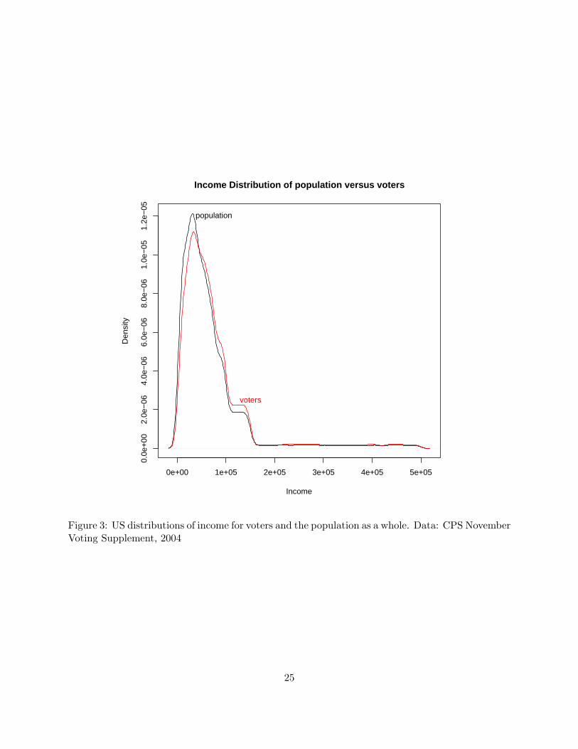
The main finding of this project is that the income distribution of voters does not differ much

from that of the income distribution of the population as a whole. Figure 3 shows the two distribu-

tions for the year 2004. While there is slight evidence that voters are better off than the population

(as evidenced by greater mass in the region of income just above $100,000, and slightly less in

the region from about $10,000 to $60,000, the overall picture is one of little difference. Figure 4

shows a quantile-quantile plot of the incomes of voters, the population as a whole, and non-voters.

here again we see that up to around the 90th percentile, the income of voters tracks that of the

population as a whole very closely. The income of non-voters is somewhat lower at each quantile,

8

but the smaller number of non-voters (this survey has turnout reported at rates of about 72%)

accounts for the non-symmetry of the deviations. The convergence of incomes at the very top of

the distribution may be an artifact of top-coding in the data, but the important aspect of the figure

for our purposes is how little difference there is in the bulk of the distribution. Differences in the

top decile are less important because the relevant piece of the model that is affected by turnout is

the income of the median voter, which is fairly robust to differences if the top tail. The sensitivity

of the mean to top incomes does not matter since the relevant measure of mean income is the mean

income of all taxpayers, and this is not changed by turnout.

The Income Distribution of Voters in Comparative Perspective

Calculating the income distributions of voters in different countries presents some serious data

problems. The best data on income (the LIS) contains no information on voting, and nor do

many other standard sources of data. The relevant information could probably be compiled from

national data sources, but there would remain questions of comparable. The approach taken here is

designed to be suggestive only, given that the measures I have of turnout are very imperfect. I use

the ISSP Role of Government III (1996) [21] to calculate distributions of income for 21 countries

for which the data are available. The ISSP does not actually ask directly about whether the

respondent voted in the last election. Thus the measures I use are somewhat indirect. The first is

the question that asks of people who did not vote, what their reason for non voting was. Those

who did vote are coded as such. Thus I use this an an indicator of voting. The second measure

uses the question asking respondents for whom they cast their vote in the last election. Again,

this question includes a response indicating that the respondent did not vote, which provides my

indicator variable. In some countries only one of these two variables is available. The resulting

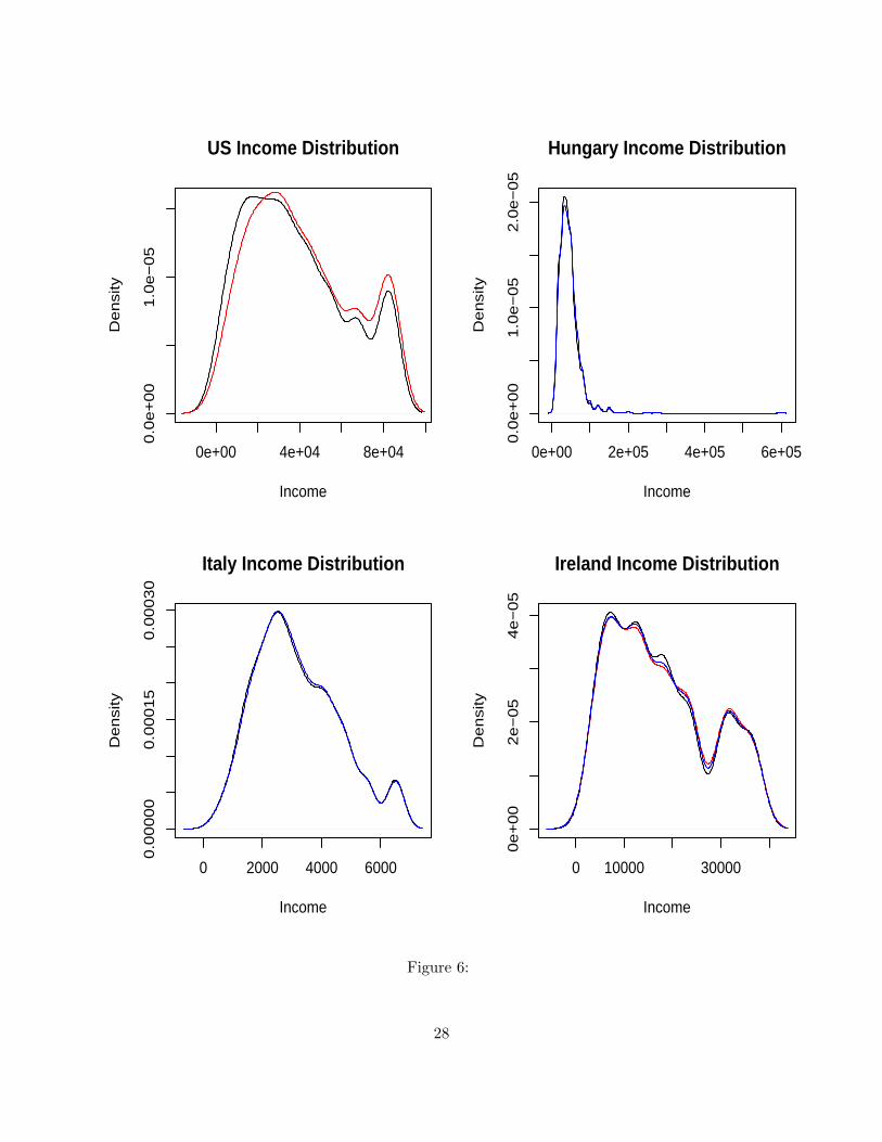
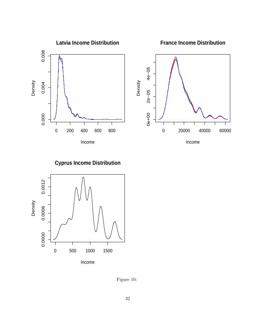
distributions are displayed in Figures 5,6,7,8,9 and 10. Again, the most striking feature of these

distributions is the similarities of the population distributions and the distributions only including

those who vote. The one exception to this seems to be the US, where the distribution of voters

does in fact seem to be shifted fairly significantly rightwards. However, given the limitations of

these data, those from the CPS seem more convincing. However, this discrepancy may be worth

further investigation.

9

Meltzer-Richard Implications: US State Spending in Time-Series Cross Section

Due to the limited data on cross-national income distributions of voters as compared to non-voters,

the primary test of the Meltzer-Richard model that I have pursued using the appropriate income

distribution (mean minus median voter income) measure is a time series, cross-sectional analysis

of US states. The magnitude of the CPS survey allows for reasonable estimates of the inequality

parameter from the micro-data, aggregated at the state level. I use the November Voter Supple-

ments of the Current Population Survey [7] from 1972 to 2000 to simulate a population for each

election year, for the population as a whole and for those who responded that they voted in the

election that year. For each election year, for each state, I draw a number of individuals in pro-

portion to the size of the income bracket in the survey (the CPS typically contains 14 gradations

of income in the November survey. The CPS March files also contain reports of income in exact

dollar amounts, but due to higher levels of non-response, and artificial clustering around ‘round’

numbers ($0, $10000 and $20000 in particular) in these reports, I prefer the bracketed measures.

The distributions calculated from the brackets lead to the straightforward calculation the measure

of skew that is the relevant inequality parameter in the Meltzer-Richard model, by subtracting

the median income in the simulated population from the mean income. The measure of mean

income used is the same in both cases- the mean income in the population as a whole, since even

those who do not vote pay taxes. The median voter’s income is taken from the population of voters

only. I also construct the ‘naive’ measure of skew, not corrected for voting behavior, for comparison.

The drawback of comparing states as opposed to nations is the potential for a lack of variation

on the dependent variable. However, the individual U.S. states are responsible for two of the most

important programs of redistribution, Supplemental Security Income (SSI) and ‘welfare’: Aid to

Families with Dependent Children (AFDC) and Temporary Aid to Needy Families (TANF) after

1996. These programs constitute a significant proportion of the redistributive effort made in the

United States, and there is considerable variation in the generosity of benefits across states. In 2004

the average monthly TANF payment to a family with three children was $420, but levels ranged

from $170 to $923 [26]. There is also a large degree of variation in total state expenditure. Since

this captures all the services provided by the state, to the extent that these are ‘lump sum’ benefits

paid for through proportional taxation, this is a better measure of the ‘redistribution’ that the

10

Meltzer-Richard model seeks to explain. Thus this is my preferred measure, even though it may be

less ‘redistributive’, as commonly understood, than the more targeted public welfare expenditures.

Thus I estimate the model with these two measures of the dependent variable: per capita state

spending on public welfare, and total state government expenditure per capita. The difference be-

tween the two measures is that the latter includes many public goods which are not direct transfers

to individuals. Not all of these will benefit the poor, (spending on highways, for example) but the

additional spending will tend to be redistributive for two reasons. First, the direct intuition from

the Meltzer-Richard model, is that any benefit provided equally to all and financed from a progres-

sive tax is redistributive. Second, the poor may benefit more from public goods which are provided

in equal measure to all, since the rich are more likely to take advantage of private substitutes. In

particular, expenditures for housing and community development, parks and recreation, education,

health and hospitals are expenditures included in total spending which are likely to benefit the poor

disproportionately. In terms of adhering directly to the terms of the theoretical model, the total

expenditure model is to be preferred, since it is precisely these lump-sum benefits which the model

concerns. Public welfare spending, by contrast, is likely to be targeted to those poorer than the

median voter, and thus exhibit a different logic with respect to voting and inequality than the one

envisaged by the model. However, this latter variable captures everyday notions of ‘redistribution’

better than the broader expenditure measure, thus I include results for both variables. The data

for both of these variables come from the Statistical Abstract of the United States [8] for various

years, as do the data on the proportion of the population over age 65 and the unemployment rate.

In contrast to the limited variation that the US states may provide on the dependent variable,

to some extent this kind of comparison may be more tenable since the maintained assumption that

the relationships between the variables (whatever they turn out to be) are in fact generated by the

same underlying processes is easier to defend given more similar units of observation. The second

important implicit assumption in using a pooled cross-section is that the relevant relationships

are constant across time. Since the theory relating inequality to redistribution is highly abstract,

and is relies predominantly on the assumption that individuals are trying to maximize their in-

come, this aspect does not seem too problematic (although there is a literature on the emergence

11

of post-materialist voting [20], much recent scholarship [28],[3] indicates that the importance of

voting according to economic interests has not declined in the U.S. However, there is one caveat.

The benefits of redistribution to the median voter depends on the efficiency of the taxation system,

as the disincentive effects of high marginal rates for the rich may limit output, harming even the

poorest in the population. Thus if the system of taxation has become more efficient over time

(efficient in the technical sense of raising the same revenue for a smaller cost in terms of output

foregone), this could undermine the assumption of a stable relationship over time, which would

render pooling the repeated cross sections inappropriate. Arguably this has indeed been the case

in the U.S. in the last thirty years. I will ignore this potential spoiler for now.

The model I estimate is a multivariate one, where for each state (indexed i = 1, ..., N) for each

year (indexed t = 1, ..., T ), redistributive spending is given by:

yit = α + φyi,t−1 + β1(inequality)it + βXit + εit,

where the βXit are the relevant control variables that must be included to isolate the relationship

between inequality and redistribution. Ideally, given the theoretical model, the model would be

estimated in levels. However, since all the variables show some degree of non-stationarity over time,

this presents a problem. My initial time-series analyses could not reject the null hypotheses that

each of the variables is non-stationary in levels, nor did they show evidence of cointegration at

traditional significance levels. Differencing the variables resulted in data that can be well modeled

by stationary time series, but this implies investigating the relationships between changes in the

independent variables and dependent variables:

∆yit = α + φ∆yi,t−1 + β1(∆inequality)it + β∆Xit + εit.

I present the results of both models, noting that while the models in changes are much to be

preferred from a statistical standpoint, they do depart from the exact scope of the theoretical

model.

I follow the literature and Beck and Katz (1995)[4] and use ordinary least squares regression (OLS)

with panel corrected standard errors. To account for the time-dependency of the outcome variable,

12

the lagged dependent variable is included in the right hand side. One lag turns out to be ensure that

the errors are (conditionally) temporally independent, which is no that surprising given that one lag

in the dependent variable is a lag of two years. Given the dimensions of the data (N = 50, T = 16),

such methods specifically for time-series cross-sectional data perform usually better and almost

never worse than econometric methods used in panel data. For the sake of robustness checking,

I also estimate the model in levels using a lest squares dummy variables (LSDV) estimator. The

model is:

yit = αi + φyi,t−1 + β1(inequality)it + βXit + εit.

The LSDV estimator allows for heterogeneity in means for each state, constant through time, by

including a series of dummy variables for each geographical unit. This estimator is biased, since it

effectively demeans the variables using a mean estimated from all the time periods, introducing a

correlation between the demeaned lagged dependent variable and the demeaned error term. How-

ever, in terms of trading off bias and root mean squared error, in typical TSCS data the LSDV

estimator outperforms many alternative estimators (see Beck and Katz (2004) and the references

therein)[5].

The matrix of control variables in each case includes: gross state product per capita; union mem-

bers as a percentage of non-agricultural wage and salary workers (including public sector workers);

the unemployment rate; the proportion of the population older than 65 years; and the proportion

of the state’s population that is African American. State product is included to capture the effects

of ‘Wagner’s Law’ that growing government expenditure is a result of economic progress. Union

membership has been shown to be important in the determination of the size of welfare states

cross-nationally: the differential mobilization and organization of labor being a key explanatory

variable in the power resources theory of welfare state development [25]. The data for gross state

product come from the Bureau of Economic Analysis [2], and is estimated as the sum of the costs

incurred and incomes earned in the states’ production divided by the population of the state in

the same year, while data on union membership come from Hirsch, MacPhereson and Vroman’s

estimates from the CPS [18].

13

The other key variable in power resources theory is the political power of socialist or leftist

parties in government [19]. In my initial analyses I included a dummy variable for the partisanship

of the incumbent governor leading up to the election-year observation. However, it never had any

significant effect, thus I omit it in the results presented here. Furthermore, there are theoretical

reasons to doubt that U.S. partisan incumbency would have the same important effect on redis-

tributive effort, as compared to the parties in Western Europe, which is the focus of the literature

that finds an important effect. First, neither of the American parties can truly be characterized as

a party of the left, or a social democratic party, and it is the incumbency of social democrats which

is found to be important in the European literature. Second, political parties in the U.S. are far less

cohesive, coherent entities than their European counterparts [23]. This is particularly pronounced

at the state level, since to be a Democrat in one state or region can mean a very different plat-

form from the party platform of another state’s Democratic party. This is particularly pronounced

with respect to the historical difference between Northern and Southern democrats, but it remains

a more general point. Divergence in party strategies within the parties makes incumbency a far

weaker predictor of outcomes.

The unemployment rate is likely to be positively related to redistribution for mechanical reasons:

as unemployment increases, the population eligible to receive transfer benefits is likely to increase.

For this reason it is included as a control. Note though that this effect is likely to be much stronger

in the cases of transfers and public welfare expenditure than in total expenditures, which are less

likely to have this mechanism at work, and may remain stable as other projects are cut to finance

higher levels of unemployment. Similarly, since much government spending is directed toward the

elderly, an increasing elderly population may increase expenditure. At the state level this is less

pronounced than federal expenditure (the latter includes the bulk of Social Security and Medicare

expenditure), but nevertheless SSI and other medical spending are two examples of why a large

elderly population is likely to lead to greater spending. Demographic change may also have a more

complicated effect. Since the elderly are disproportionately likely to vote than the population as

a whole, a higher proportion of elderly people may lead to different patterns in the relationship

between voting and income than we would otherwise expect, and perhaps increase political pressure

for redistribution (if the elderly are more likely to be poorer) as well as working via the mechanical

14

effect on expenditures. On the other hand, a high proportion of elderly residents has been shown

to depress education spending, particularly when the children receiving schooling are of a different

ethnic group than the elderly [34]. Thus the effect of the proportion elderly may depend on the

nature of redistributive spending.

Finally, I include the proportion of the state population that is African-American to capture

the possibility that this diversity affects redistributive generosity. Alesina and Glaeser [1] maintain

that a large portion of the difference between US redistributive effort and the higher levels found in

Western Europe is accounted for by greater racial diversity in America, and that this association is

repeated at the state level in the United States. Austen-Smith and Wallerstein demonstrate that

this outcome can prevail even when people have ‘color-blind’ preferences, where affirmative action

is an alternative to redistribution as a policy dimension in aid of minorities [10]. There is also a

strong relationship in American public opinion, which reveals little support for welfare when it is

associated with African American recipients [14].

One other variable which is accorded some importance in the international comparative litera-

ture is the degree of openness of the economy to international trade and competition. Katzenstein

[24] argues that small, open economies develop industrial policies to shelter workers from the higher

risks that international exposure brings. However, the accuracy of this link is disputed convincingly

by Rodrik [36], and while data are available on international trade, the relevant risks that state-level

policy would need to insure, under this argument, include the risks associated with higher levels of

inter-state trade within the U.S. In the absence of such data I do not include this variable in the

analysis.

Results

As outlined above, I estimate two different specifications (changes and levels), and two different es-

timators (OLS and LSDV), for both of the dependent variables (public welfare spending per capita

and total state expenditure per capita). Each of these is estimated using both the naive measure of

skew and the measure corrected for turnout. The results are very similar across the two estimators

15

thus I do not report those for the LSDV estimator. Across the two estimators the significance and

magnitude of the coefficients on inequality are qualitatively identical. The only difference is that

the effects of unemployment and population over 65 are no longer significant in the LSDV models

estimated in levels. This is likely because they trend only very gradually through time and this

variation is captured by the unit-specific means. Overall, the results are fairly consistent across

specifications, and indicate that while inequality thus measured may have a statistically significant

positive effect on government spending on redistribution, the substantive magnitude of the effect is

tiny. Tables 1 and 2 present the regression results.

The tables show coefficients which represent the effect in dollars on the dependent variable of a

$1000 change in GSP per capita, the lagged dependent variable or the measures of skewness, and

for a 1% change in either unionization, the unemployment rate or the proportion of the population

over 65 years of age. There are a few notable things about the results with respect to the control

variables. First, GSP per capita has the predicted sign in all cases, and is significant in three of

the four specifications for both measures of inequality (models 1c, 1d, 2a,2b,2c and 2d). That

it has no effect in the models for changes in public welfare spending is not that surprising when

we consider that in periods of growth, there are fewer people in need of public welfare spending,

although increased tax receipts, among other things, ensure that total expenditure still rises. In

terms of levels, however, variation in unemployment comes less from year-to-year growth but from

differences across states, and here therefor it is the case that richer states are able to provide more

generous benefits, in accordance with Wagner’s Law. Unionization rates are significant in only

two of the eight models, and are signed inconsistently in the remaining six. The absence of strong

union pressure for higher levels of redistributive spending may be a result of the weakness of U.S.

labor in general, such that even in highly unionized states members cannot push for benefits to

labor as has been shown to be the case in Europe. Alternatively it may be that even where unions

remain numerically strong in the period since 1972 they limit their demands on governments in the

face of increasingly hostile attitudes of business and the public at large. Of course, much of this is

speculation and making the argument that this is indeed the case would be a task for future research.

Unemployment has a consistently positive and significant effect on public welfare spending, but

16

not on general expenditures; this is in line with theoretical predictions. The proportion of elderly

people in the population is complicated, confirming the ambiguous theoretical predictions. First,

it is the only coefficient that is sensitive to the inclusion of the proportion of African Americans in

the state, which coincides with Poterba’s findings on education spending. In models 1a and b, and

2a, b, c, and d, the proportion of old people in the population has a negatively signed coefficient,

and in the models estimated in changes it is a large effect. This may be accounted for by the fact

that most state-level spending is not directed toward the elderly, but rather provides education and

transfers to younger people. The effect of the size of the black population of the state runs counter

to theoretical prediction when considering changes, but is in accordance with the theoretical lit-

erature when considering levels. This could be due to some lags in timing, however it might also

point to a mis-specification of the model, particularly given the distinctiveness of the American

South in terms both of redistribution and black population. The levels effect of proportion black

may be picking up an anti-redistributive legacy of Southern institutions and attitudes rather than

the mechanisms identified in the theoretical discussion.

The lagged dependent variable is significant in levels for both dependent variables, but insignif-

icant in estimating changes. The interpretation of the coefficient on the lagged dependent variable

in changes is that it measures the extent to which a change in expenditure is followed by a continued

change (in the same direction), thus is is not too surprising that it is not an important variable in

these specifications. In levels, the conclusion that high spending in one year leads to high spending

the next is unsurprising, but the lagged dependent variable is necessary to model the temporal

dependence in the data. the coefficients on unemployment are interesting, as its effects are consis-

tently significant and positive in determining public welfare spending per capita, and consistently

negative but insignificant in predicting total expenditure. One possible explanation for this would

be that there is a mechanical translation of higher unemployment to higher direct transfers, since

more people are eligible for benefits, but at the same time unemployment limits state resources,

which ultimately must come from taxation, and thus constrains total expenditure.

However, the important results for testing the Meltzer-Richard model are the coefficients on

the inequality measures. There are three aspects to these results. First, inequality is generally

17

significant and positive, as predicted. Second, however, it is consistently associated with only a

tiny substantive effect, despite being precisely estimated. For a $1000 increase in the rate of change

of inequality, the rate of change of public welfare spending increases by about one-tenth of a cent.

Alternatively in levels, an increase of $1000 in the difference between the mean income and that

of the median voter, total expenditure per capita increases by one and a half cents. The average

rate of change of Meltzer-Richard skew from one period to the next is $3663, this amounts to an

average increase of less than half a cent per period in increasing the rate of change of public welfare

spending, and four and a half cents in the rate of increase of total spending. The estimates from the

models in levels indicate that moving from the 25th to the 75th percentile inequality levels (a move

of one and a quarter standard deviations of that variable) would lead to only a $412 increase in total

expenditure, 0.2 standard deviations of the dependent variable. Third, and most importantly for

this project, there is never any qualitative difference between the naive measure of inequality and

the measure correcting for turnout. All of these results are fairly robust to the model specification.

Meltzer-Richard Implications: Preferences on Redistribution in Comparative

Perspective

One advantage of the ISSP data in considering the effect of turnout on the preferences of the median

voter is that it does allow us to directly consider preferences rather than redistributive outcomes,

which are likely to be affected by many other factors also. These factors (unionization, left party

government etc) may still be important, but is likely to be less important for the determination of

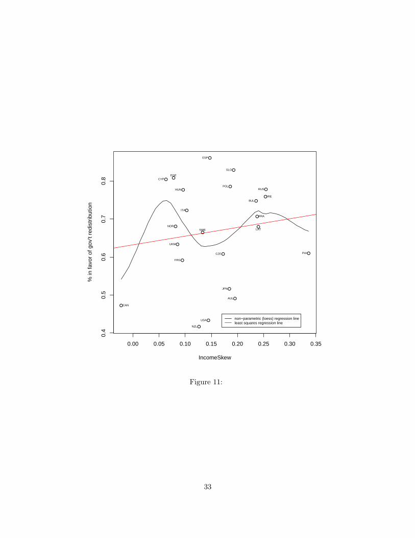
preferences than in determining actual redistribution. Figure 11 shows the effect of income skew on

population level preferences. The dependent variable here is the percentage of respondents within

the country answering “definitely should be” or “probably should be” to the question

On the whole, do you think it should be or should not be the governments responsibility

to: Reduce income differences between the rich and poor.

The figure reveals a positive relationship between inequality and support for redistribution, as pre-

dicted by the Meltzer-Richard model, but there is wide variation around this trend, and further

the relationship appears to be non-linear. This non-linearity seems to be driven by the fact that,

by these measures of inequality, the USA, New Zealand, Australia and Japan score in the middle

18

range on inequality and have low support for redistribution.

Figures 12 and 13 show the difference between the preferences of the median income individual

and the median income voter, by two measures. Figure 12 shows the percentage of individuals

in the median income quintile who support government redistribution, analogous to the aggregate

measure.This figure does provide support for the contention that turnout makes the difference to

the Meltzer-Richard model: for the population as a whole, support for redistribution is (albeit very

weakly) increasing in the skew of income. However in the right hand panel where only those who

voted are considered, the relationship does become negative (and also support for redistribution is

generally lower). However, this result is not robust to a slightly different definition of the median.

Figure 13 shows the average answer to the same question as above from all voters who report in-

come equal to the median income (population or voters) in their country, where the response that

the government “definitely should” reduce income differences between rich and poor is coded as 4,

“probably should” as 3, “probably should not” as 2, and “definitely should not” as 1. Here the

positive relationship between income skew and preferences over redistribution is amplified when

turnout is taken into account.

The overall impression of these results is that, on the whole, turnout cannot account for the

discrepancy between the Meltzer-Richard model and empirical observation. However, the results in

terms of preferences actually show exactly the relationship that the Meltzer-Richard model predicts.

Thus it may be worth considering that the ‘demand side’ of the Meltzer-Richard model, operating

from the distribution of income to individual level preferences (and the preferences of the median

voter) holds, but it is on the policy ‘supply side’ that the model fails. That is, the translation of

preferences into policy is where the simplifying assumptions of the Meltzer-Richard model are too

restrictive.

Discussion, Conclusion

In conclusion, it seems that unequal turnout does not provide the explanation for the Robin Hood

paradox, since there is little difference between the income distributions of those who vote as com-

pared to the populations they represent. This is not the fatal assumption in the Meltzer-Richard

19

model.

However, in trying to investigate this across countries, I find that the Meltzer-Richard effect of

inequality increasing redistribution, does seem to hold in the context of individual preferences over

policy. Thus it is likely in the translation from preferences to policy that the ‘problem’ with the

Meltzer-Richard model emerges. This is hardly surprising given the lack of any model of politics

in the model. These results also indicate that unequal voter turnout is hardly ‘democracy’s unre-

solved dilemma’, since the preferences, and outcomes based on the voter population are unaffected

by explicitly modeling turnout. Nevertheless, some ‘dilemma’ remains, to the extent that if the

preliminary findings here- that preferences do track the predictions of the Meltzer-Richard model-

hold, then the lack of congruence between these preferences and policy outcomes raises questions

as to how these preferences are aggregated and channeled into policy.

20

Figures & Tables

1a 1b 1c 1dChanges Changes Levels Levels

Intercept 58.5*** 57.8*** −60.9*** −60.0***(5.4) (5.4) (17.6) (17.7)

M-R Skew .00089** −.00019(.0004) (.0003)

Naive Skew .00092** −.00013(.0004) (.0003)

GSP/capita 0.68 0.86 2.9*** 2.8***(1.9) (1.9) (.59) (.61)

Unionization (%) 3.7** 3.7** −.38 −.40(1.7) (1.7) (.32) (.32)

Unemployment (%) 7.5*** 7.8*** 4.3*** 4.4***(1.7) (1.7) (1.3) (1.2)

Population 65+ (%) −25.0*** −25.0*** 3.8*** 3.8(9.5) (9.5) (1.0) (1.1)

Population Black (%) 22.4*** 22.3*** −0.23 −0.24(6.5) (6.6) (0.26) (0.27)

Lagged DV 26.7 26.8 1010*** 1009***(45.7) (45.5) (23.0) (23.2)

Table 1: OLS estimates. Dependent Variable (DV) is Public Welfare Spending per Capita. Inde-pendent variables in 000s, except proportions. Panel Corrected Standard Errors in parentheses.Significance levels: *** 0.01, ** 0.05, * 0.1.

21

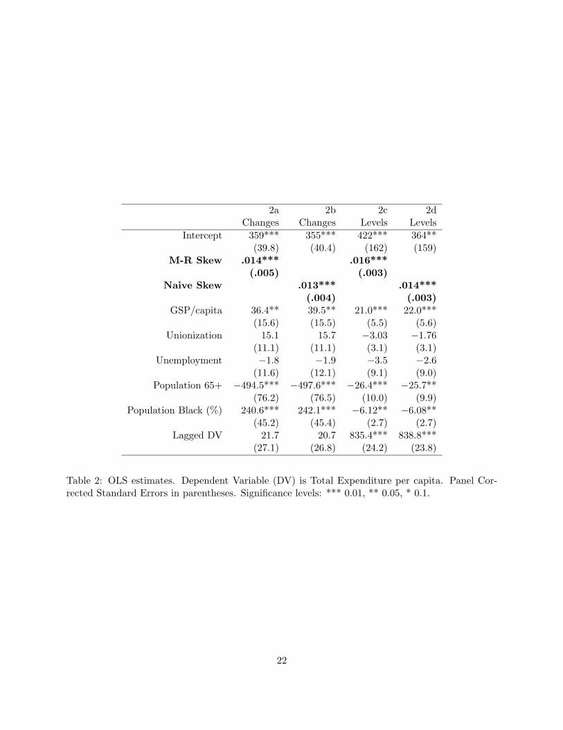
2a 2b 2c 2dChanges Changes Levels Levels

Intercept 359*** 355*** 422*** 364**(39.8) (40.4) (162) (159)

M-R Skew .014*** .016***(.005) (.003)

Naive Skew .013*** .014***(.004) (.003)

GSP/capita 36.4** 39.5** 21.0*** 22.0***(15.6) (15.5) (5.5) (5.6)

Unionization 15.1 15.7 −3.03 −1.76(11.1) (11.1) (3.1) (3.1)

Unemployment −1.8 −1.9 −3.5 −2.6(11.6) (12.1) (9.1) (9.0)

Population 65+ −494.5*** −497.6*** −26.4*** −25.7**(76.2) (76.5) (10.0) (9.9)

Population Black (%) 240.6*** 242.1*** −6.12** −6.08**(45.2) (45.4) (2.7) (2.7)

Lagged DV 21.7 20.7 835.4*** 838.8***(27.1) (26.8) (24.2) (23.8)

Table 2: OLS estimates. Dependent Variable (DV) is Total Expenditure per capita. Panel Cor-rected Standard Errors in parentheses. Significance levels: *** 0.01, ** 0.05, * 0.1.

22

Figure 1: In the basic model, the median voter is ‘automatically’ determined by individual income.In model B, who the median is will depend on who turns out to vote. This will mean that thepreferences of the actual median voter may not be the preferences of the individual with medianincome. The latter we would still expect to be increasing in equality, but the effect of inequalityon the former would depend on how inequality affects turnout and the income bias to turnout.Thus we would see a divergences of the preferences of the MV from the median person. This is incontrast to a model where voting is egalitarian but the rich have other ways to influence policy.There the bias toward the rich would intervene between ‘median voter preferences’ and ‘policy’,and we would not necessarily see a divergence of preferences between the median voter and themedian individual. 23

2 3 4 5 6 7

0.0

0.2

0.4

0.6

0.8

Income Distribution of Voters versus Economic Agents

Income

Den

sity

Distribution of Voters

Distribution of Economic Agents

Y*YM YMV

Figure 2: The Difference Between Median Income and Median Voter Income in (Approximate)Skewed Normal Distributions Where Income of Voters is More Skewed than Population Income.Y M is median income of the population, Y ∗ is population mean income, and Y MV is the incomeof the median voter.

24

0e+00 1e+05 2e+05 3e+05 4e+05 5e+05

0.0e

+00

2.0e

−06

4.0e

−06

6.0e

−06

8.0e

−06

1.0e

−05

1.2e

−05

Income Distribution of population versus voters

Income

Den

sity

population

voters

Figure 3: US distributions of income for voters and the population as a whole. Data: CPS NovemberVoting Supplement, 2004

25

●●●●●●●●●●●●●●●●●●●●●●

●●●●●●●●●●●●●●●●●●●●●●●●

●●●●●●●●●●

●●●●●●●●●●

●●●●●●●●●●

●●●●●●

●●●●●●●●●●●

●

●

●

●

●

●

●

0e+00 1e+05 2e+05 3e+05 4e+05 5e+05

0e+

001e

+05

2e+

053e

+05

4e+

055e

+05

q.pop

q.vo

t

●●●●●●●●●●●●●●

●●●●●●●●●●●●●●●●

●●●●●●●●●●●●●●●●

●●●●●●●●●●●●●●●

●●●●●●●●●●

●●●●●●●●

●●●●●●●●●●●●●●

●●

●●

●

●

●

●●●●●●●●●●●●●●

●●●●●●●●●●●●●●●●●●

●●●●●●●●●●●●●

●●●●●●●●●●

●●●●●●●●●●

●●●●●●●●

●●●●●●

●●●●●●

●●

●●●

●●

●●

●

●

●

●

●

●

●●●●●●●●●●●●●●

●●●●●●●●●●●●●●●●

●●●●●●●●●●●●●●●●

●●●●●●●●●●●●●●●

●●●●●●●●●●

●●●●●●●●

●●●●●●●●●●●●●●

●●

●●

●

●

●

●●●●●●●●●●●●●●

●●●●●●●●●●●●●●●●●●

●●●●●●●●●●●●●

●●●●●●●●●●

●●●●●●●●●●

●●●●●●●●

●●●●●●

●●●●●●

●●

●●●

●●

●●

●

●

●

●

●

●

non−voters

voters

Figure 4: Quantile-quantile plot of incomes: population versus voters and non-voters. Data: CPSNovember VotingSupplement, 2004. Note that the real divergence between voters and non-voters(and the population as a whole) occurs only at the very highest quantiles of the distribution- aboveabout the 90th percentile.

26

0e+00 2e+05 4e+05 6e+05

0.0

e+

00

1.0

e−

05

Australia Income Distribution

Income

De

nsi

ty

0 5000 15000 25000

0.0

00

00

0.0

00

10

0.0

00

20

W.Ger Income Distribution

IncomeD

en

sity

0 5000 10000 15000

0.0

00

00

0.0

00

15

0.0

00

30

E.Ger Income Distribution

Income

De

nsi

ty

0 10000 30000 50000

0e

+0

02

e−

05

4e

−0

5

Great Britain Income Distribution

Income

De

nsi

ty

Figure 5: Black lines indicate the distribution of income in the population as a whole; red lines thedistribution of those classified as voters by the ‘reasons for not voting’ question; blue lines thosewho voted according to the ‘what party did you vote for’ question.

27

0e+00 4e+04 8e+04

0.0

e+

00

1.0

e−

05

US Income Distribution

Income

De

nsi

ty

0e+00 2e+05 4e+05 6e+05

0.0

e+

00

1.0

e−

05

2.0

e−

05

Hungary Income Distribution

IncomeD

en

sity

0 2000 4000 6000

0.0

00

00

0.0

00

15

0.0

00

30

Italy Income Distribution

Income

De

nsi

ty

0 10000 30000

0e

+0

02

e−

05

4e

−0

5

Ireland Income Distribution

Income

De

nsi

ty

Figure 6:

28

0e+00 4e+05 8e+05

0.0

e+

00

1.0

e−

06

2.0

e−

06

Norway Income Distribution

Income

De

nsi

ty

0 10000 20000 30000 40000

0e

+0

02

e−

05

4e

−0

5

Sweden Income Distribution

IncomeD

en

sity

0 40000 80000 120000

0e

+0

04

e−

05

8e

−0

5

Czech Income Distribution

Income

De

nsi

ty

0e+00 4e+05 8e+05

0e

+0

02

e−

06

4e

−0

66

e−

06

Slovenia Income Distribution

Income

De

nsi

ty

Figure 7:

29

0 2000 4000 6000 8000

0e

+0

04

e−

04

Poland Income Distribution

Income

De

nsi

ty

0e+00 2e+05 4e+05 6e+05

0e

+0

02

e−

06

4e

−0

6

Bulgaria Income Distribution

IncomeD

en

sity

0 2000 6000 10000

0e

+0

04

e−

04

Russia Income Distribution

Income

De

nsi

ty

0 40000 80000 120000

0.0

e+

00

6.0

e−

06

1.2

e−

05

New Zealand Income Distribution

Income

De

nsi

ty

Figure 8:

30

0e+00 4e+04 8e+04

0.0

e+

00

1.0

e−

05

Canada Income Distribution

Income

De

nsi

ty

0e+00 4e+04 8e+04

0.0

00

00

0.0

00

06

0.0

00

12

Phillipines Income Distribution

IncomeD

en

sity

0 5000 10000 15000

0.0

00

00

0.0

00

06

0.0

00

12

Japan Income Distribution

Income

De

nsi

ty

0e+00 4e+05 8e+05

0e

+0

04

e−

06

8e

−0

6

Spain Income Distribution

Income

De

nsi

ty

Figure 9:

31

0 200 400 600 800

0.0

00

0.0

04

0.0

08

Latvia Income Distribution

Income

De

nsi

ty

0 20000 40000 60000

0e

+0

02

e−

05

4e

−0

5

France Income Distribution

IncomeD

en

sity

0 500 1000 1500

0.0

00

00

.00

06

0.0

01

2

Cyprus Income Distribution

Income

De

nsi

ty

Figure 10:

32

●

●

●

●

●

●

●

●

●

●

●

●

●

●

●

●

●

●

●

●

●

●

●

0.00 0.05 0.10 0.15 0.20 0.25 0.30 0.35

0.4

0.5

0.6

0.7

0.8

IncomeSkew

% in

favo

r of

gov

't re

dist

ribut

ion

AUL

FRG

EGE

UKM

USA

HUN

ITA

IRE

NORSWE

CZE

SLO

POL

BUL

RUS

NZL

CAN

PHI

JPN

ESP

LAT

FRA

CYP

non−parametric (loess) regression lineleast squares regression line

Figure 11:

33

●

●

●

●

●●

●

●

●

●

●

●

●

●

●

●

●

●

●

0.00 0.10 0.20 0.30

0.2

0.3

0.4

0.5

0.6

0.7

0.8

0.9

IncomeSkew

% o

f med

ian in

com

e qu

intile

in fa

vor o

f gov

't red

istrib

ution

AUL

FRG

EGE

UKM

USAHUN

ITA

NOR

CZE

SLO

POL

BUL

RUS

NZL

PHI

JPN

ESP

LAT

FRA

●

●

●

●

●

●

●

●

●

●

●

●

●

●

●

●

●

●

●

0.00 0.10 0.20 0.30

0.2

0.3

0.4

0.5

0.6

0.7

0.8

0.9

IncomeSkew

% o

f med

ian in

com

e qu

intile

(vot

ers)

in fa

vor o

f gov

't red

istrib

ution

AUL

FRG

EGE

UKM

USA

HUN

ITA

NOR

CZE

SLO

POL

BUL

RUS

NZL

PHI

JPN

ESP

LAT

FRA

Figure 12:

34

●

●

●

●

●

●

●

●

●●

●

●

●

●

●

●●

●

●

●

●●

●

0.00 0.10 0.20 0.30

1.0

1.5

2.0

2.5

3.0

3.5

4.0

IncomeSkew

med

ian in

com

e ind

ividu

al's p

refe

renc

e on

gov

't red

istrib

ution

AUL

FRG

EGE

UKM

USA

HUN

ITA

IRE

NORSWE

CZE

SLO

POL

BUL

RUS

NZLCAN

PHI

JPN

ESP

LAT

FRA

CYP

●

●

●

●

●

●

●●

●

●

●

●

●

●

●●

●●

●

●●●

0.00 0.10 0.20 0.30

1.0

1.5

2.0

2.5

3.0

3.5

4.0

IncomeSkew

med

ian in

com

e vo

ter's

pre

fere

nce

on g

ov't r

edist

ribut

ionAUL

FRG

UKM

USA

HUN

ITA

IRENOR

SWE

CZE

SLO

POL

BUL

RUS

NZLCAN

PHIJPN

ESP

LATFRA

CYP

Figure 13:

35

References

[1] Alberto Alesina and Edward L. Glaeser. Fighting Poverty in the US and Europe. Oxford:

Oxford University Press, 2004.

[2] U.S. Department Of Commerce: Bureau Of Economic Analysis. Regional economic accounts.

http://www.bea.gov/bea/regional/gsp. Accessed 5 July 2006. Last Revised 6 June 2006.

[3] Larry M. Bartels. What’s the matter with ’what’s the matter with kansas’? Quarterly Journal

Of Political Science, 1(2), 2006.

[4] Nathaniel Beck and Jonathan N. Katz. What to do (and not to do) with time-series cross-

section data. American Political Science Review, 89(3), 1995.

[5] Nathaniel Beck and Jonathan N. Katz. Time-series cross-sections: Dynamics, 2004. Paper Pre-

sented To The Annual Meeting Of The Society For Political Methodology, Stanford University,

2004.

[6] Bennett and Resnick. The implications of nonvoting for democracy in the united states.

American Journal of Political Science, 34(3), 1990.

[7] United States Department Of Commerce: Bureau Of The Census. Current population

survey:voter supplement files, 1972-2002. 1972: hdl:1902.2/00060http://id.thedata.org/

hdl%3a1902.2%2f00060; 1974: hdl:1902.2/07558http://id.thedata.org/hdl%3a1902.

2%2f07558; 1976:hdl:1902.2/07699http://id.thedata.org/hdl%3a1902.2%2f07699;

1978:hdl:1902.2/07876http://id.thedata.org/hdl%3a1902.2%2f07876; 1980:hdl:

1902.2/07875http://id.thedata.org/hdl%3a1902.2%2f07875; 1982:hdl:1902.2/

08193http://id.thedata.org/hdl%3a1902.2%2f08193; 1984:hdl:1902.2/08457http:

//id.thedata.org/hdl%3a1902.2%2f08457; 1986:hdl:1902.2/08707http://id.thedata.

org/hdl%3a1902.2%2f08707; 1988:hdl:1902.2/09318http://id.thedata.org/hdl%

3a1902.2%2f09318; 1990:hdl:1902.2/09715http://id.thedata.org/hdl%3a1902.2%

2f09715; 1992:hdl:1902.2/06365http://id.thedata.org/hdl%3a1902.2%2f06365;

1994:hdl:1902.2/06548http://id.thedata.org/hdl%3a1902.2%2f06548; 1996:hdl:

1902.2/02205http://id.thedata.org/hdl%3a1902.2%2f02205; 1998:hdl:1902.2/

02803http://id.thedata.org/hdl%3a1902.2%2f02803; 2000:hdl:1902.2/03182http:

36

//id.thedata.org/hdl%3a1902.2%2f03182; 2002:hdl:1902.2/03967http://id.thedata.

org/hdl%3a1902.2%2f03967.

[8] U.S. Department Of Commerce: Bureau Of The Census. Statistical abstract of the united

states: Various years. http://www.census.gov/compendia/statab/past years.html.

[9] Citrin, Schickler, and Sides. What if everyone voted? simulating. the impact of increased

turnout in senate elections. American Journal of Political Science, 47(1), 2003.

[10] Austen-Smith David and Michael Wallerstein. Redistribution and affirmative action. North-

western University, typescript, 2004.

[11] J de Nardo. Turnout and the vote - the joke’s on the democrats. American Political Science

Review, 74(2), 1980.

[12] Robert J Franzese Jr. Political participation, income distribution and public transfers in devel-

oped democracies. Paper Presented To The American Political Science Association, September,

2000.

[13] Gant and Lyons. Democratic theory, nonvoting, and public policy: The 1972-88 presidential

elections. American Political Quarterly, 21(2), 1993.

[14] Martin Gilens. Why Americans Hate Welfare: Race, Media and the Politics of Anti-Poverty

Policy. Chicago: University of Chicago Press, 1999.

[15] Alexander M Hicks and Duane H. Swank. Politics, institutions and welfare spending in indus-

trialized democracies, 1960-1982. American Political Science Review, 86(3), 1992.

[16] Highton and Wolfinger. The political implications of higher voter turnout. British Journal of

Political Science, 31(1), 2001.

[17] Kim Quaile Hill and Jan E. Leighley. The policy consequences of class bias in state electorates.

American Journal Of Political Science, 36(2), 1992.

[18] Barry T. Hirsch, David A. Macpherson, and Wayne G. Vroman. Estimates of union density

by state. Monthly Labor Review, 124(7), 2001.

37

[19] Evelyne Huber and John D Stephens. Development And Crisis Of The Welfare State: Parties

And Policies In Global Markets. Chicago: University Of Chicago Press, 2001.

[20] Ronald F. Inglehart. The silent revolution: Intergenerational change in post-industrial soci-

eties. American Political Science Review, 65(4), 1971.

[21] International Social Survey Program (ISSP). 1999-10-07: International social survey program:

Role of government iii, 1996. hdl:1902.2/02808http://id.thedata.org/hdl%3A1902.2%

2F02808. Inter-university Consortium for Political and Social Research [distributor(DDI)].

[22] Torben Iversen and Anne Wren. Equality, employment and budgetary constraint: The

trilemma of the service economy. World Politics, 50(4), 1998.

[23] Richard S. Katz and Robin Kolodny. Party organization as an empty vessel: Parties in am-

reican politics. In Richard S. Katz and Peter Mair, editors, How Parties Organize: Change

And Adaptation In Party Organizations In Western Democracies. London: Sage Publications,

1994.

[24] Peter Katzenstein. Small States In World Markets: Industrial Policy In Europe. Cornell

University Press, 1985.

[25] Walter Korpi. The Democratic Class Struggle. London: Routledge, 1983.

[26] Ed Lazere and Chris Tallent. Not enough to live on. Dc Fiscal Policy Institute, 2006.

[27] Arend Lijphart. Unequal participation: Democracy’s unresolved dilemma. American Political

Science Review, 91(1), 1997.

[28] Nolan M Mccarty, Keith T. Poole, and Howard Rosenthal. Income Redistribution And The

Realignment Of American Politics. Washington D.C: The Aei Press, 1997.

[29] Allan H Meltzer and Scott F. Richard. Tests of a rational theory of the size of government.

Public Choice, 41(3), 1983.

[30] Allen H. Meltzer and Scott F. Richard. A rational theory of the size of government. Journal

Of Political Economy, 89(5), 1981.

38

[31] Nagel and McNulty. Partisan effects of voter turnout in senatorial and gubernatorial elections.

American Political Science Review, 90(4), 1996.

[32] Alexander Pacek and Benjamin Radcliff. Turnout and the vote for left-of-centre parties: A

cross- national analysis. British Journal Of Political Science, 25(1), 1995.

[33] Roberto Perotti. Growth, income distribution and democracy: What the data say. Journal

Of Economic Growth, 1, 1996.

[34] James M. Poterba. Demographich structure and the political economy of public education.

Journal of Policy Analysis and Management, 16(1), 1998.

[35] Francisco Rodriguiez C. Does distributional skewness lead to redistribution? evidence from

the united states. Economics And Politics, 11(2), 1999.

[36] Dani Rodrik. Has Globalization Gone Too Far? Washington DC:Institute For International

Economics, 1997.

[37] Sidney Verba, Norman H. Nie, and Jae-On Kim. Participation And Political Equality. Cam-

bridge, England:Cambridge University Press, 1978.

[38] Raymond E Wolfinger and Steven J. Rosenstone. Who Votes? New Haven: Yale University

Press, 1980.

39