MNRAS 465, 105–110 (2017) doi:10.1093/mnras/stw2770Advance Access publication 2016 October 28

Does turbulence determine the initial mass function?

David Liptai,1‹ Daniel J. Price,1 James Wurster1,2 and Matthew R. Bate2

1School of Physics and Astronomy, Monash University, Clayton, VIC 3800, Australia2School of Physics, University of Exeter, Stocker Road, Exeter EX4 4QL, UK

Accepted 2016 October 25. Received 2016 October 24; in original form 2016 August 28

ABSTRACTWe test the hypothesis that the initial mass function (IMF) is determined by the densityprobability distribution function (PDF) produced by supersonic turbulence. We compare 14simulations of star cluster formation in 50 M! molecular cloud cores where the initial turbu-lence contains either purely solenoidal or purely compressive modes, in each case resolvingfragmentation to the opacity limit to determine the resultant IMF. We find statistically indis-tinguishable IMFs between the two sets of calculations, despite a factor of 2 difference in thestar formation rate and in the standard deviation of log (!). This suggests that the density PDF,while determining the star formation rate, is not the primary driver of the IMF.

Key words: brown dwarfs – stars: formation – stars: low-mass – stars: luminosity function,mass function.

1 IN T RO D U C T I O N

Two decades of theoretical studies have established that a lognormaldensity probability distribution function (PDF) is the defining char-acteristic of supersonic turbulence (e.g. Vazquez-Semadeni 1994;Nordlund & Padoan 1999; Ostriker, Gammie & Stone 1999; Klessen2000; Kritsuk et al. 2007; see review by Elmegreen & Scalo 2004).In particular, numerous studies (e.g. Padoan, Nordlund & Jones1997a; Lemaster & Stone 2008; Price, Federrath & Brunt 2011;Molina et al. 2012) have shown that the density variance is propor-tional to the Mach number, giving

" 2ln ! = ln

!1 + b2M2" , (1)

where " ln ! is the standard deviation in the logarithm of the density(i.e. the ‘width’ of the PDF), M is the root-mean-square (RMS)Mach number and b is a constant of order unity related to themixture of solenoidal and compressive modes in the velocity field(e.g. Federrath, Klessen & Schmidt 2008; Federrath et al. 2010).

Padoan & Nordlund (2002) proposed that the PDF determines theIMF for low-mass stars (M < 1 M!), based on the observation thatthe IMF is also lognormal at the low-mass end (e.g. Chabrier 2003,2005). Relating the PDF to the IMF is powerful because it enablesanalytic theories of star formation (e.g. Krumholz & McKee 2005;Hennebelle & Chabrier 2008, 2009; Hopkins 2012; Guszejnov &Hopkins 2015) which predict the IMF from the few parameters inequation (1). Relating the initial mass function (IMF) to the statisticsof turbulence explains the universal nature of the IMF in the MilkyWay (e.g. Bastian, Covey & Meyer 2010), since nearby molecularclouds show supersonic motions with seemingly universal scaling

# E-mail: david.liptai@monash.edu

relations (Zuckerman & Evans 1974; Larson 1981; Heyer & Brunt2004).

Measurements of lognormal column density PDFs from extinc-tion mapping (Lombardi, Alves & Lada 2006; Lombardi, Lada &Alves 2008, 2010) lend support to a direct relationship between thePDF and the IMF. In particular, Kainulainen et al. (2009) showedthat star-forming clouds differ from non-star-forming clouds by thepresence of a power-law tail in the column density PDF at high den-sities, suggesting that self-gravity merely converts the high-densityend of the PDF into stars. The measured mass function of ‘cores’also seems to mimic the stellar IMF, but shifted to higher masses,implying a one-to-one relationship between ‘cores’ and ‘stars’ withan efficiency factor of "0.3 (e.g. Motte, Andre & Neri 1998; Testi &Sargent 1998; Luhman & Rieke 1999; Johnstone et al. 2000; Alves,Lombardi & Lada 2007; Nutter & Ward-Thompson 2007; Enochet al. 2008; Rathborne et al. 2009; Chabrier & Hennebelle 2010).However, numerous studies have also cautioned or argued againsta direct core mass function and IMF relationship (e.g. Ballesteros-Paredes et al. 2006; Goodwin et al. 2008; Smith, Clark & Bonnell2008, 2009).

Alternatively, Bonnell et al. (1997) and Bate & Bonnell (2005)proposed that the IMF is determined by ‘competitive accretion’between low-mass fragments for a limited gas supply, with accretiontruncated by the preferential ejection of low-mass stars and browndwarfs from unstable multiple systems. This was demonstrated inthe star cluster formation calculations of Bate, Bonnell & Bromm(2003; hereafter BBB03). These were the first attempts to simulatethe IMF ‘directly’ by resolving the gravitational collapse to theopacity limit for fragmentation (the density at which radiation istrapped by dust, ! # 10$13 g cm$3, implying an increase rather thandecrease in the Jeans mass with density, and hence the formation ofa single hydrostatic object; Low & Lynden-Bell 1976; Rees 1976).

C% 2016 The AuthorsPublished by Oxford University Press on behalf of the Royal Astronomical Society

at University of Exeter on D

ecember 13, 2016

http://mnras.oxfordjournals.org/

Dow

nloaded from

106 D. Liptai et al.

Sink particles were inserted in the calculations once the opacity limitwas reached, enabling simulation of the subsequent accretion up tothe final stellar masses. This approach has had remarkable success atreproducing the observed IMF, with the most recent calculation byBate (2012) modelling the formation of 183 stars and brown dwarfsfrom a 500 M! cloud, finding an IMF statistically indistinguishablefrom the local IMF compiled by Chabrier (2005).

While these simulations employ turbulent clouds, it is not obvioushow the resultant IMF relates to the details of the initial turbulence.A subsequent study by Bate (2009c) found no change in the IMFwhen the slope of the power spectrum of the initial turbulencewas varied. In their simple model to explain the IMF produced bysimulations, Bate & Bonnell (2005) invoke the PDF only indirectly,via a lognormal distribution of mass accretion rates. Nevertheless,a connection may still exist.

Here, we investigate the PDF–IMF connection by simulating starformation in two initially identical sets of model clouds, set up witheither purely solenoidal or purely compressive initial velocity fields.If the PDF determines the IMF, then we expect the IMFs to differ,since the PDFs should be very different. If the IMF is more due tonurture than nature, the effect may be more minor. The main caveatto our study is that we assume impulsive rather than continuousturbulent driving.

Girichidis et al. (2011) performed a related study, along with othervariations in the initial conditions, and found that the shape of theIMF was unaffected by the type of turbulent driving. However, theysimulated more massive and denser clouds (M = 100 M! and R =0.1 pc) and did not resolve to the opacity limit (sinks were insertedat a scale of 40 au, compared to 5 au employed here and in BBB03).We also perform a statistical study with multiple realizations of theinitial velocity field in each case, compared to their single realiza-tion. Lomax, Whitworth & Hubber (2015) recently compared theeffect of solenoidal versus compressive forcing in star formation cal-culations, but focused on smaller cores (M = 3 M!; R = 3000 au),examining the effect on disc and binary fractions rather than theIMF.

While this paper was under review, an important and comple-mentary study to ours was published by Bertelli Motta et al. (2016),examining the correlation between the IMF and the statistics ofturbulence using two sets of simulations where the turbulence wasfirst driven to a steady state in a periodic box before ‘switching on’gravity. These authors varied the Mach number as well as the den-sity of the cloud, using a total mass of either 5750 M! or 516 M!in a 10 pc3 or 3 pc3 domain, respectively. Their ‘high density’ sim-ulations were resolved only to a density of 1.6 & 10$14 g cm$3, oneorder of magnitude less than the opacity limit, with sink particleradii of 100 au. They found no correlation between the Mach num-ber and the characteristic mass of the resulting IMF, concluding thatthe IMF is mainly determined by small-scale processes such as discformation and fragmentation and not by turbulence driven at thescale of the cloud. However, studying the role of initial conditionsin a clump with decaying turbulence remains important since thismay be closer to the situation in dense cores prior to the onset ofstellar feedback.

2 N U M E R I C A L M E T H O D

We use the PHANTOM smoothed particle hydrodynamics (SPH) code(Lodato & Price 2010; Price & Federrath 2010; Price 2012). Thisis the first application of PHANTOM to star cluster formation.

2.1 Initial conditions

Aside from the initial velocity fields, our setup is identical to thatin BBB03: we set up a series of turbulent, spherical clouds, with50 M! of gas of uniform density with diameter 0.375 pc. Thecorresponding initial free-fall time is tff = 1.90 & 106 yr. Theminimum Jeans mass at the opacity limit is Mmin # 0.0011 M!.We use 3.5 million SPH particles, consistent with BBB03, whoshowed that about 75 particles are required per Mmin (see also Bate& Burkert 1997). Particles were distributed in a uniform randomdistribution. We adopt code units with a length unit of 0.1pc, massunit of 1 M! and time units such that G = 1.

2.2 Equation of state

We adopt a barotropic equation of state P = K!$ . Following BBB03,we prescribe $ = 1 (i.e. isothermal) for densities lower than theopacity limit for fragmentation (! = 10$13 gcm$3), $ = 7/5 for10$13 gcm$3 < ! < 10$10 gcm$3 and $ = 1.1 for ! > 10$10 gcm$3.We define the constant K to be such that the sound speed is cs =1.84 & 104 cm s$1 during the isothermal phase (i.e. 10 K assuminga mean molecular weight µ = 2.46) and in the $ = 7/5 regimesuch that the pressure remains continuous when $ changes. Asdiscussed by Bate (2009a), using a barotropic equation of stateoverproduces low-mass stars and brown dwarfs compared to ob-servations, since the cold gas surrounding the protostars fragmentstoo readily (cf. Fig. 6). Several groups (Bate 2009b, 2012; Offneret al. 2009; Commercon et al. 2010; Krumholz et al. 2010) showedthat this can be solved by modelling radiation in the flux-limiteddiffusion approximation. However, simulations with radiation areexpensive, precluding the kind of statistical study we perform here,the radiation algorithm is not yet implemented in PHANTOM, anda barotropic equation of state is sufficient to answer the questionof whether the PDF influences the IMF. We also ignore magneticfields which change the star formation rate and perhaps also the IMF(Ostriker et al. 1999; Heitsch, Mac Low & Klessen 2001; Vazquez-Semadeni, Kim & Ballesteros-Paredes 2005; Tilley & Pudritz 2007;Price & Bate 2008, 2009; Myers et al. 2014).

2.3 Velocity fields: solenoidal versus compressive driving

We impulsively drive turbulence in each cloud, as in BBB03, by im-posing an initial supersonic turbulent velocity field. The amplitudeof the velocity fluctuations follow a power spectrum P(k) ' k$4,where k is the wavenumber, in order to be consistent with Larson’sscaling relation. We generate each field via a Fourier transform ona 643 grid, which is then interpolated on to the SPH particles. Thecoefficient of each Fourier mode is drawn from a Rayleigh distri-bution with each mode also given a uniform random phase between[$ !, !]. This is equivalent to sampling from a cylindrical bivariateGaussian (Dubinski, Narayan & Phillips 1995).

To obtain a purely solenoidal velocity field, we take the curl ofa vector field to produce a divergence-free velocity field. Similarlyfor a purely compressive velocity field, we take the gradient of ascalar field to produce a curl-free field. We compute the gradientsin Fourier space. Velocities are normalized so that the initial kineticenergy is equal to the gravitational potential energy, giving an ini-tial RMS Mach number of M = 6.4. We performed simulationsusing seven realizations of the initial velocity field for each case(solenoidal or compressive), realized by changing the seed in therandom number generator for the phases and amplitudes.

MNRAS 465, 105–110 (2017)

at University of Exeter on D

ecember 13, 2016

http://mnras.oxfordjournals.org/

Dow

nloaded from

Does the PDF lead to the IMF? 107

Figure 1. Evolution of column density during the gravitational collapse of two example 50 M! molecular cloud cores with purely solenoidal (top) and purelycompressive (bottom) initial turbulent velocity fields. The large-scale structure of the clouds is very different, with the compressive case showing a factor of 2increase in the standard deviation of log (!) compared to the solenoidal case as well as stronger shocks and a faster onset to star formation. To obtain enoughstatistics to determine the IMF, we perform simulations using seven realizations of each type of driving, giving 14 simulations in total.

2.4 Sink particles

Following BBB03, we introduce sink particles (Bate, Bonnell &Price 1995) when the central density of pressure-supported frag-ments reaches !s = 10$11 g cm$3, two orders of magnitude higherthan the opacity limit. Once !s is exceeded and sink formationconditions are satisfied, we replace gas particles within 5 au witha sink particle. Gas particles within 5 au are accreted if they passchecks for angular momentum and boundness, with their mass andmomentum added to the sink. Gravity between sinks is softenedwithin 4 au; gas particles are accreted without checks within thisradius.

3 R ESULTS

3.1 Column density evolution

Fig. 1 shows the evolution of column density from t = 0 to t = 0.3tff

(left to right) in two representative calculations, using solenoidaldriving (top, as in BBB03) and compressive driving (bottom).Shocks form quickly in both cases, due to the impulsive super-sonic velocity field, but are stronger in the compressive case, driv-ing the formation of large-scale filaments after only 0.3tff. For thesolenoidal case, ( · v = 0 initially by definition, so there are noregions which initially promote collapse.

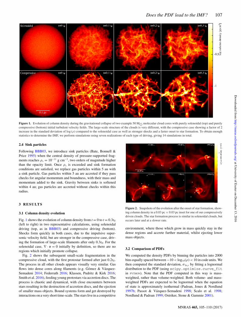
Fig. 2 shows the subsequent small-scale fragmentation in thecompressive cloud, with the first protostar formed after just 0.2tff.The process in all other clouds appears visually very similar. Gasflows into dense cores along filaments (e.g. Gomez & Vazquez-Semadeni 2014; Federrath 2016; Klassen, Pudritz & Kirk 2016;Smith et al. 2016), feeding young protostars via accretion discs. Theprocess is chaotic and dynamical, with close encounters betweenstars resulting in the destruction of accretion discs, and the ejectionof smaller mass objects. Bound systems form and get destroyed byinteractions on a very short time-scale. The stars live in a competitive

Figure 2. Snapshots of the evolution after the onset of star formation, show-ing column density in a 0.03 pc & 0.03 pc inset for one of our compressivelydriven clouds. The star formation process is similar in solenoidal clouds, butoccurs later and at a slower rate.

environment, where those which grow in mass quickly stay in thedense regions and accrete further material, whilst ejecting lowermass objects.

3.2 Comparison of PDFs

We computed the density PDFs by binning the particles into 2000bins equally spaced between $10 < log10(!) < 10 in code units. Wethen computed the standard deviation, " ln ! by fitting a lognormaldistribution to the PDF (using scipy.optimize.curve_fitin PYTHON). Note that the PDF computed in this way is mass-weighted, rather than volume-weighted. Both volume- and mass-weighted PDFs are expected to be lognormal when the equationof state is approximately isothermal (Padoan, Jones & Nordlund1997b; Passot & Vazquez-Semadeni 1998; Scalo et al. 1998;Nordlund & Padoan 1999; Ostriker, Stone & Gammie 2001).

MNRAS 465, 105–110 (2017)

at University of Exeter on D

ecember 13, 2016

http://mnras.oxfordjournals.org/

Dow

nloaded from

108 D. Liptai et al.

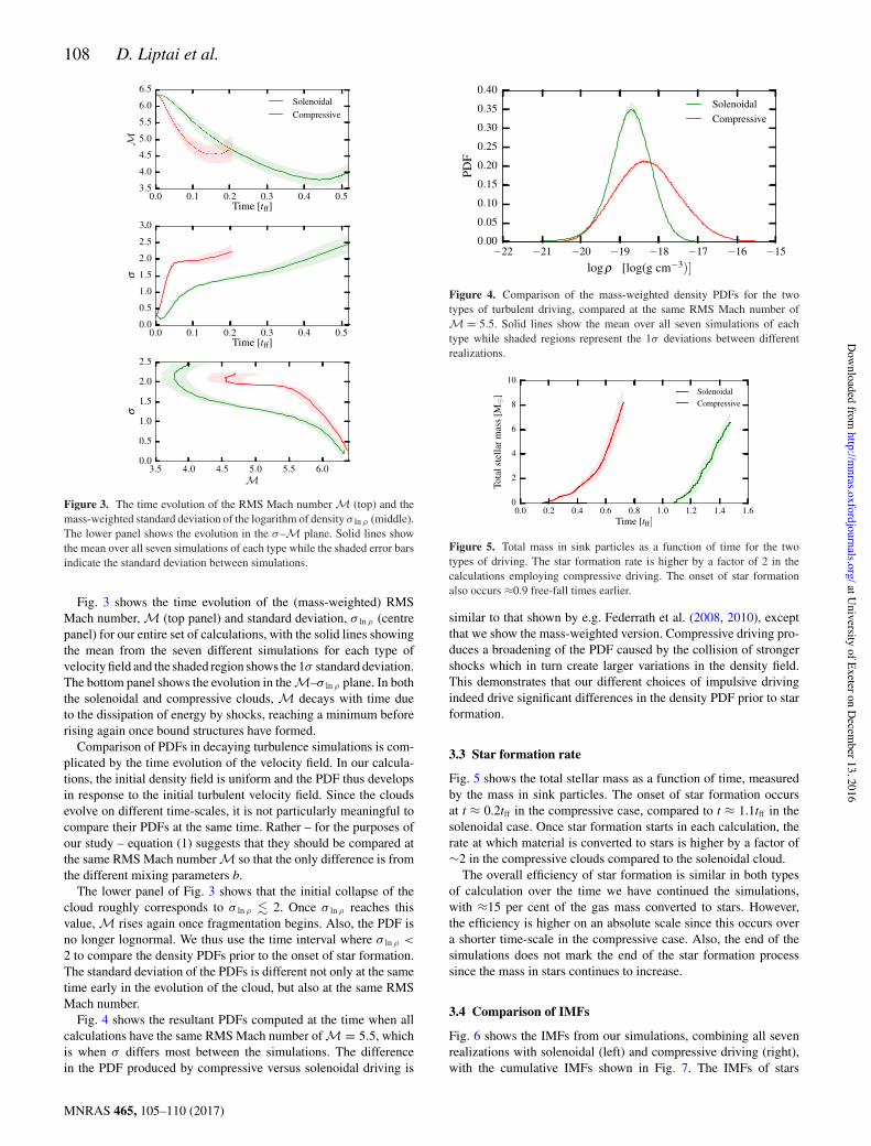
Figure 3. The time evolution of the RMS Mach number M (top) and themass-weighted standard deviation of the logarithm of density " ln ! (middle).The lower panel shows the evolution in the "–M plane. Solid lines showthe mean over all seven simulations of each type while the shaded error barsindicate the standard deviation between simulations.

Fig. 3 shows the time evolution of the (mass-weighted) RMSMach number, M (top panel) and standard deviation, " ln ! (centrepanel) for our entire set of calculations, with the solid lines showingthe mean from the seven different simulations for each type ofvelocity field and the shaded region shows the 1" standard deviation.The bottom panel shows the evolution in the M–" ln ! plane. In boththe solenoidal and compressive clouds, M decays with time dueto the dissipation of energy by shocks, reaching a minimum beforerising again once bound structures have formed.

Comparison of PDFs in decaying turbulence simulations is com-plicated by the time evolution of the velocity field. In our calcula-tions, the initial density field is uniform and the PDF thus developsin response to the initial turbulent velocity field. Since the cloudsevolve on different time-scales, it is not particularly meaningful tocompare their PDFs at the same time. Rather – for the purposes ofour study – equation (1) suggests that they should be compared atthe same RMS Mach number M so that the only difference is fromthe different mixing parameters b.

The lower panel of Fig. 3 shows that the initial collapse of thecloud roughly corresponds to " ln ! ! 2. Once " ln ! reaches thisvalue, M rises again once fragmentation begins. Also, the PDF isno longer lognormal. We thus use the time interval where " ln ! <

2 to compare the density PDFs prior to the onset of star formation.The standard deviation of the PDFs is different not only at the sametime early in the evolution of the cloud, but also at the same RMSMach number.

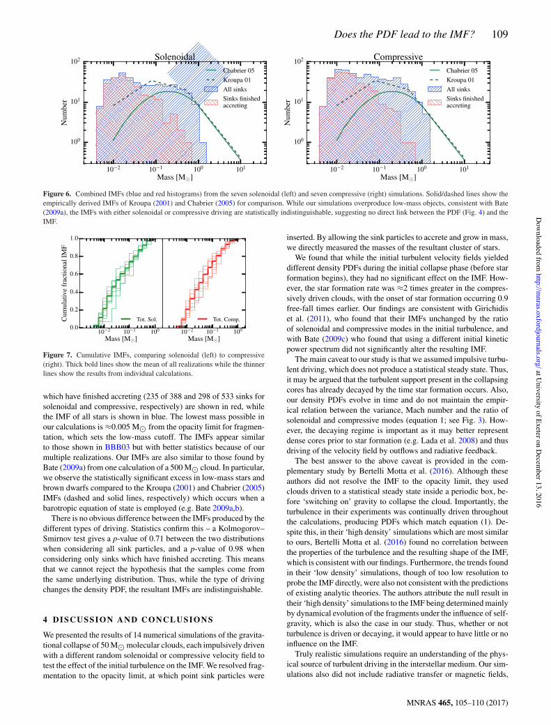
Fig. 4 shows the resultant PDFs computed at the time when allcalculations have the same RMS Mach number of M = 5.5, whichis when " differs most between the simulations. The differencein the PDF produced by compressive versus solenoidal driving is

Figure 4. Comparison of the mass-weighted density PDFs for the twotypes of turbulent driving, compared at the same RMS Mach number ofM = 5.5. Solid lines show the mean over all seven simulations of eachtype while shaded regions represent the 1" deviations between differentrealizations.

Figure 5. Total mass in sink particles as a function of time for the twotypes of driving. The star formation rate is higher by a factor of 2 in thecalculations employing compressive driving. The onset of star formationalso occurs #0.9 free-fall times earlier.

similar to that shown by e.g. Federrath et al. (2008, 2010), exceptthat we show the mass-weighted version. Compressive driving pro-duces a broadening of the PDF caused by the collision of strongershocks which in turn create larger variations in the density field.This demonstrates that our different choices of impulsive drivingindeed drive significant differences in the density PDF prior to starformation.

3.3 Star formation rate

Fig. 5 shows the total stellar mass as a function of time, measuredby the mass in sink particles. The onset of star formation occursat t # 0.2tff in the compressive case, compared to t # 1.1tff in thesolenoidal case. Once star formation starts in each calculation, therate at which material is converted to stars is higher by a factor of"2 in the compressive clouds compared to the solenoidal cloud.

The overall efficiency of star formation is similar in both typesof calculation over the time we have continued the simulations,with #15 per cent of the gas mass converted to stars. However,the efficiency is higher on an absolute scale since this occurs overa shorter time-scale in the compressive case. Also, the end of thesimulations does not mark the end of the star formation processsince the mass in stars continues to increase.

3.4 Comparison of IMFs

Fig. 6 shows the IMFs from our simulations, combining all sevenrealizations with solenoidal (left) and compressive driving (right),with the cumulative IMFs shown in Fig. 7. The IMFs of stars

MNRAS 465, 105–110 (2017)

at University of Exeter on D

ecember 13, 2016

http://mnras.oxfordjournals.org/

Dow

nloaded from

Does the PDF lead to the IMF? 109

Figure 6. Combined IMFs (blue and red histograms) from the seven solenoidal (left) and seven compressive (right) simulations. Solid/dashed lines show theempirically derived IMFs of Kroupa (2001) and Chabrier (2005) for comparison. While our simulations overproduce low-mass objects, consistent with Bate(2009a), the IMFs with either solenoidal or compressive driving are statistically indistinguishable, suggesting no direct link between the PDF (Fig. 4) and theIMF.

Figure 7. Cumulative IMFs, comparing solenoidal (left) to compressive(right). Thick bold lines show the mean of all realizations while the thinnerlines show the results from individual calculations.

which have finished accreting (235 of 388 and 298 of 533 sinks forsolenoidal and compressive, respectively) are shown in red, whilethe IMF of all stars is shown in blue. The lowest mass possible inour calculations is #0.005 M! from the opacity limit for fragmen-tation, which sets the low-mass cutoff. The IMFs appear similarto those shown in BBB03 but with better statistics because of ourmultiple realizations. Our IMFs are also similar to those found byBate (2009a) from one calculation of a 500 M! cloud. In particular,we observe the statistically significant excess in low-mass stars andbrown dwarfs compared to the Kroupa (2001) and Chabrier (2005)IMFs (dashed and solid lines, respectively) which occurs when abarotropic equation of state is employed (e.g. Bate 2009a,b).

There is no obvious difference between the IMFs produced by thedifferent types of driving. Statistics confirm this – a Kolmogorov–Smirnov test gives a p-value of 0.71 between the two distributionswhen considering all sink particles, and a p-value of 0.98 whenconsidering only sinks which have finished accreting. This meansthat we cannot reject the hypothesis that the samples come fromthe same underlying distribution. Thus, while the type of drivingchanges the density PDF, the resultant IMFs are indistinguishable.

4 D I S C U S S I O N A N D C O N C L U S I O N S

We presented the results of 14 numerical simulations of the gravita-tional collapse of 50 M! molecular clouds, each impulsively drivenwith a different random solenoidal or compressive velocity field totest the effect of the initial turbulence on the IMF. We resolved frag-mentation to the opacity limit, at which point sink particles were

inserted. By allowing the sink particles to accrete and grow in mass,we directly measured the masses of the resultant cluster of stars.

We found that while the initial turbulent velocity fields yieldeddifferent density PDFs during the initial collapse phase (before starformation begins), they had no significant effect on the IMF. How-ever, the star formation rate was #2 times greater in the compres-sively driven clouds, with the onset of star formation occurring 0.9free-fall times earlier. Our findings are consistent with Girichidiset al. (2011), who found that their IMFs unchanged by the ratioof solenoidal and compressive modes in the initial turbulence, andwith Bate (2009c) who found that using a different initial kineticpower spectrum did not significantly alter the resulting IMF.

The main caveat to our study is that we assumed impulsive turbu-lent driving, which does not produce a statistical steady state. Thus,it may be argued that the turbulent support present in the collapsingcores has already decayed by the time star formation occurs. Also,our density PDFs evolve in time and do not maintain the empir-ical relation between the variance, Mach number and the ratio ofsolenoidal and compressive modes (equation 1; see Fig. 3). How-ever, the decaying regime is important as it may better representdense cores prior to star formation (e.g. Lada et al. 2008) and thusdriving of the velocity field by outflows and radiative feedback.

The best answer to the above caveat is provided in the com-plementary study by Bertelli Motta et al. (2016). Although theseauthors did not resolve the IMF to the opacity limit, they usedclouds driven to a statistical steady state inside a periodic box, be-fore ‘switching on’ gravity to collapse the cloud. Importantly, theturbulence in their experiments was continually driven throughoutthe calculations, producing PDFs which match equation (1). De-spite this, in their ‘high density’ simulations which are most similarto ours, Bertelli Motta et al. (2016) found no correlation betweenthe properties of the turbulence and the resulting shape of the IMF,which is consistent with our findings. Furthermore, the trends foundin their ‘low density’ simulations, though of too low resolution toprobe the IMF directly, were also not consistent with the predictionsof existing analytic theories. The authors attribute the null result intheir ‘high density’ simulations to the IMF being determined mainlyby dynamical evolution of the fragments under the influence of self-gravity, which is also the case in our study. Thus, whether or notturbulence is driven or decaying, it would appear to have little or noinfluence on the IMF.

Truly realistic simulations require an understanding of the phys-ical source of turbulent driving in the interstellar medium. Our sim-ulations also did not include radiative transfer or magnetic fields,

MNRAS 465, 105–110 (2017)

at University of Exeter on D

ecember 13, 2016

http://mnras.oxfordjournals.org/

Dow

nloaded from

110 D. Liptai et al.

both of which play an important role in determining the IMF. Fur-thermore, our ability to probe the IMF at M " 1 M! is limited bythe 50 M! total mass of our model clouds. Worthwhile follow-upstudies would include radiative feedback and more massive clouds(e.g. Bate 2012; Krumholz, Klein & McKee 2012) and magneticfields (e.g. Myers et al. 2014).

ACKNOWLEDGEMENTS

We thank the anonymous referee for comments which have im-proved the paper. We acknowledge CPU time on gSTAR, fundedby Swinburne University and the Australian Government. Thisproject was funded via Australian Research Council DiscoveryProject DP130102078 and Future Fellowship FT130100034. Weused SPLASH (Price 2007).

R E F E R E N C E S

Alves J., Lombardi M., Lada C. J., 2007, A&A, 462, L17Ballesteros-Paredes J., Gazol A., Kim J., Klessen R. S., Jappsen A.-K.,

Tejero E., 2006, ApJ, 637, 384Bastian N., Covey K. R., Meyer M. R., 2010, ARA&A, 48, 339Bate M. R., 2009a, MNRAS, 392, 590Bate M. R., 2009b, MNRAS, 392, 1363Bate M. R., 2009c, MNRAS, 397, 232Bate M. R., 2012, MNRAS, 419, 3115Bate M. R., Bonnell I. A., 2005, MNRAS, 356, 1201Bate M. R., Burkert A., 1997, MNRAS, 288, 1060Bate M. R., Bonnell I. A., Price N. M., 1995, MNRAS, 277,

362Bate M. R., Bonnell I. A., Bromm V., 2003, MNRAS, 339, 577 (BBB03)Bertelli Motta C., Clark P. C., Glover S. C. O., Klessen R. S., Pasquali A.,

2016, MNRAS, 462, 4171Bonnell I. A., Bate M. R., Clarke C. J., Pringle J. E., 1997, MNRAS, 285,

201Chabrier G., 2003, PASP, 115, 763Chabrier G., 2005, Astrophys. Space Sci. Libr., 327, 41Chabrier G., Hennebelle P., 2010, ApJ, 725, L79Commercon B., Hennebelle P., Audit E., Chabrier G., Teyssier R., 2010,

A&A, 510, L3Dubinski J., Narayan R., Phillips T. G., 1995, ApJ, 448, 226Elmegreen B. G., Scalo J., 2004, ARA&A, 42, 211Enoch M. L., Evans N. J., II, Sargent A. I., Glenn J., Rosolowsky E., Myers

P., 2008, ApJ, 684, 1240Federrath C., 2016, MNRAS, 457, 375Federrath C., Klessen R. S., Schmidt W., 2008, ApJ, 688, L79Federrath C., Roman-Duval J., Klessen R. S., Schmidt W., Mac Low M.-M.,

2010, A&A, 512, A81Girichidis P., Federrath C., Banerjee R., Klessen R. S., 2011, MNRAS, 413,

2741Gomez G. C., Vazquez-Semadeni E., 2014, ApJ, 791, 124Goodwin S. P., Nutter D., Kroupa P., Ward-Thompson D., Whitworth A. P.,

2008, A&A, 477, 823Guszejnov D., Hopkins P. F., 2015, MNRAS, 450, 4137Heitsch F., Mac Low M.-M., Klessen R. S., 2001, ApJ, 547, 280Hennebelle P., Chabrier G., 2008, ApJ, 684, 395Hennebelle P., Chabrier G., 2009, ApJ, 702, 1428Heyer M. H., Brunt C. M., 2004, ApJ, 615, L45Hopkins P. F., 2012, MNRAS, 423, 2037

Johnstone D., Wilson C. D., Moriarty-Schieven G., Joncas G., Smith G.,Gregersen E., Fich M., 2000, ApJ, 545, 327

Kainulainen J., Beuther H., Henning T., Plume R., 2009, A&A, 508, L35Klassen M., Pudritz R. E., Kirk H., 2016, MNRAS, preprint

(arXiv:1605.08835)Klessen R. S., 2000, ApJ, 535, 869Kritsuk A. G., Norman M. L., Padoan P., Wagner R., 2007, ApJ, 665, 416Kroupa P., 2001, MNRAS, 322, 231Krumholz M. R., McKee C. F., 2005, ApJ, 630, 250Krumholz M. R., Cunningham A. J., Klein R. I., McKee C. F., 2010, ApJ,

713, 1120Krumholz M. R., Klein R. I., McKee C. F., 2012, ApJ, 754, 71Lada C. J., Muench A. A., Rathborne J., Alves J. F., Lombardi M., 2008,

ApJ, 672, 410Larson R. B., 1981, MNRAS, 194, 809Lemaster M. N., Stone J. M., 2008, ApJ, 682, L97Lodato G., Price D. J., 2010, MNRAS, 405, 1212Lomax O., Whitworth A. P., Hubber D. A., 2015, MNRAS, 449, 662Lombardi M., Alves J., Lada C. J., 2006, A&A, 454, 781Lombardi M., Lada C. J., Alves J., 2008, A&A, 489, 143Lombardi M., Lada C. J., Alves J., 2010, A&A, 512, A67Low C., Lynden-Bell D., 1976, MNRAS, 176, 367Luhman K. L., Rieke G. H., 1999, ApJ, 525, 440Molina F. Z., Glover S. C. O., Federrath C., Klessen R. S., 2012, MNRAS,

423, 2680Motte F., Andre P., Neri R., 1998, A&A, 336, 150Myers A. T., Klein R. I., Krumholz M. R., McKee C. F., 2014, MNRAS,

439, 3420Nordlund Å. K., Padoan P., 1999, in Franco J., Carraminana A., eds, Inter-

stellar Turbulence. Cambridge Univ. Press, Cambridge, p. 218Nutter D., Ward-Thompson D., 2007, MNRAS, 374, 1413Offner S. S. R., Klein R. I., McKee C. F., Krumholz M. R., 2009, ApJ, 703,

131Ostriker E. C., Gammie C. F., Stone J. M., 1999, ApJ, 513, 259Ostriker E. C., Stone J. M., Gammie C. F., 2001, ApJ, 546, 980Padoan P., Nordlund Å., 2002, ApJ, 576, 870Padoan P., Nordlund A., Jones B. J. T., 1997a, MNRAS, 288, 145Padoan P., Jones B. J. T., Nordlund A. P., 1997b, ApJ, 474, 730Passot T., Vazquez-Semadeni E., 1998, Phys. Rev. E, 58, 4501Price D. J., 2007, PASA, 24, 159Price D. J., 2012, J. Comput. Phys., 231, 759Price D. J., Bate M. R., 2008, MNRAS, 385, 1820Price D. J., Bate M. R., 2009, MNRAS, 398, 33Price D. J., Federrath C., 2010, MNRAS, 406, 1659Price D. J., Federrath C., Brunt C. M., 2011, ApJ, 727, L21Rathborne J. M., Lada C. J., Muench A. A., Alves J. F., Kainulainen J.,

Lombardi M., 2009, ApJ, 699, 742Rees M. J., 1976, MNRAS, 176, 483Scalo J., Vazquez-Semadeni E., Chappell D., Passot T., 1998, ApJ, 504, 835Smith R. J., Clark P. C., Bonnell I. A., 2008, MNRAS, 391, 1091Smith R. J., Clark P. C., Bonnell I. A., 2009, MNRAS, 396, 830Smith R. J., Glover S. C. O., Klessen R. S., Fuller G. A., 2016, MNRAS,

455, 3640Testi L., Sargent A. I., 1998, ApJ, 508, L91Tilley D. A., Pudritz R. E., 2007, MNRAS, 382, 73Vazquez-Semadeni E., 1994, ApJ, 423, 681Vazquez-Semadeni E., Kim J., Ballesteros-Paredes J., 2005, ApJ, 630, L49Zuckerman B., Evans N. J., II1974, ApJ, 192, L149

This paper has been typeset from a TEX/LATEX file prepared by the author.

MNRAS 465, 105–110 (2017)

at University of Exeter on D

ecember 13, 2016

http://mnras.oxfordjournals.org/

Dow

nloaded from