Does the Fed Respond to Oil Price Shocks? - Logan T. Lewis · Lutz Kilian Logan T. Lewis University...
38
0 Does the Fed Respond to Oil Price Shocks? Lutz Kilian Logan T. Lewis University of Michigan University of Michigan CEPR November 1, 2010 Abstract: Since Bernanke, Gertler and Watson (1997), a common view in the literature has been that systematic monetary policy responses to the inflation caused by oil price shocks are an important source of aggregate fluctuations in the U.S. economy, yet post-1987 data reveal no evidence of systematic policy responses to oil price shocks. Even prior to 1987, the Federal Reserve was not responding to the inflation triggered by oil price shocks, but rather to the oil price shocks directly, consistent with a preemptive move by the Federal Reserve to counteract potential inflationary pressures. There are indications that this response is poorly identified, however, and there is no evidence that this policy response in the pre-1987 period caused substantial fluctuations in the federal funds rate or in real output. One explanation of the low explanatory power of systematic policy responses to oil price shocks is that the Federal Reserve has been responding differently to different types of oil price shocks. Our analysis suggests that the traditional monetary policy reaction framework explored by BGW and incorporated in subsequent DSGE models should be replaced by DSGE models that take account of the endogeneity of the real price of oil and that allow policy responses to depend on the underlying causes of oil price shocks. JEL: E31, E32, E52, Q43, Key words: Counterfactual; Oil; Recessions; Systematic monetary policy; Policy response. Acknowledgements: We thank Mark Gertler, Ana María Herrera, Elena Pesavento and two referees for helpful discussions. Correspondence to: Lutz Kilian, Department of Economics, University of Michigan, 611 Tappan Street, Ann Arbor, MI 48109-1220. Email: [email protected] . Phone: (734) 647-5612. Fax: (734) 764-2769.
Transcript of Does the Fed Respond to Oil Price Shocks? - Logan T. Lewis · Lutz Kilian Logan T. Lewis University...

0
Does the Fed Respond to Oil Price Shocks?
Lutz Kilian Logan T. Lewis
University of Michigan University of Michigan CEPR
November 1, 2010
Abstract: Since Bernanke, Gertler and Watson (1997), a common view in the literature has been that systematic monetary policy responses to the inflation caused by oil price shocks are an important source of aggregate fluctuations in the U.S. economy, yet post-1987 data reveal no evidence of systematic policy responses to oil price shocks. Even prior to 1987, the Federal Reserve was not responding to the inflation triggered by oil price shocks, but rather to the oil price shocks directly, consistent with a preemptive move by the Federal Reserve to counteract potential inflationary pressures. There are indications that this response is poorly identified, however, and there is no evidence that this policy response in the pre-1987 period caused substantial fluctuations in the federal funds rate or in real output. One explanation of the low explanatory power of systematic policy responses to oil price shocks is that the Federal Reserve has been responding differently to different types of oil price shocks. Our analysis suggests that the traditional monetary policy reaction framework explored by BGW and incorporated in subsequent DSGE models should be replaced by DSGE models that take account of the endogeneity of the real price of oil and that allow policy responses to depend on the underlying causes of oil price shocks. JEL: E31, E32, E52, Q43,
Key words: Counterfactual; Oil; Recessions; Systematic monetary policy; Policy response.
Acknowledgements: We thank Mark Gertler, Ana María Herrera, Elena Pesavento and two referees for helpful discussions. Correspondence to: Lutz Kilian, Department of Economics, University of Michigan, 611 Tappan Street, Ann Arbor, MI 48109-1220. Email: [email protected]. Phone: (734) 647-5612. Fax: (734) 764-2769.

1
1. Introduction
Although it is common to attribute the recessions of the 1970s and early 1980s to oil price
shocks, it has proven difficult to rationalize such large real effects based on standard
macroeconomic models of the transmission of oil price shocks (see Kilian (2008a) for a review).
One channel that may help amplify the effects of oil price shocks on real output is the
endogenous policy response of the central bank to oil price shocks. Bernanke, Gertler and
Watson (1997), henceforth referred to as BGW, stipulated that the Federal Reserve, when faced
with potential or actual inflationary pressures triggered by a positive oil price shock, responds by
raising the interest rate, amplifying the decline in real output associated with oil price shocks.1 In
assessing the effect of this policy response from VAR models, BGW postulated a counterfactual
in which the Federal Reserve holds the interest rate constant. In other words, the Federal Reserve
is not responding to any of the effects of the oil price shock on the economy. BGW concluded
that the Fed's systematic and anticipated response to oil price shocks is the main cause of the
recessions that tend to follow oil price shocks and that these recessions could have been avoided
(at the cost of higher inflation) by holding the interest rate constant.2
BGW’s results have not remained unchallenged. For example, Hamilton and Herrera
(2004) showed that the estimates in BGW are sensitive to the choice of the VAR lag order.
Allowing for additional lags undermines the importance of the policy response. They also
demonstrated that implementing a constant interest rate policy would have required policy
changes so large to be unprecedented historically and hence not credible in light of the Lucas
critique, a point acknowledged by Bernanke, Gertler and Watson (2004). This evidence has done
little to diminish the appeal of BGW’s results, however.
BGW’s empirical results also have motivated a theoretical literature that examines the
potential macroeconomic impact of monetary policy responses to oil price shocks using DSGE
models. The conclusions reached in this literature very much depend on the specification of the
1 BGW viewed the monetary policy response to oil price shocks merely as a convenient example in the context of the broader question of how important systematic monetary policy responses are relative to exogenous monetary policy shocks. This example, however, has subsequently received great attention in its own right and it is this aspect of the BGW study that we focus on in this paper. 2 In the words of BGW, “an important part of the effect of oil price shocks on the economy results not from the change in oil prices, per se, but from the resulting tightening of monetary policy. This finding may help explain the apparently large effects found by Hamilton and many others.” (p. 136). They conclude that their results “provide substantial support for the view that the monetary policy response is the dominant source of the real effects of an oil price shock” (p. 124).

2
DSGE model. Whereas Leduc and Sill (2004), for example, concluded that in their DSGE model
monetary policy contributes about 40 percent to the drop in real output following a rise in the
price of oil, Carlstrom and Fuerst (2006) found that under alternative assumptions the entire
decline in real output following an oil price shock may be due to oil and none attributable to
monetary policy.3 Thus, the key question remains of how plausible the original empirical
estimates in BGW are. In this paper, we re-examine the evidence presented in BGW within the
context of the class of VAR models they employed. We build on recent insights as to the
specification of these models, we introduce additional data, and we exploit additional
econometric tools that aid in the interpretation of the model estimates.
The paper is organized as follows. In section 2, we discuss the rationale of the narrative
account presented in BGW. In section 3, we motivate and summarize the innovations in our
VAR model specification relative to BGW’s original analysis. In section 4, we analyze the
responses to oil price shocks over the periods of 1967.5-1987.7 and 1987.8-2008.6. Our analysis
of the VAR framework used in BGW implies that the Federal Reserve during the 1970s and
early 1980s responded not to actual inflation triggered by oil price shocks, but rather responded
directly to the oil price shocks, consistent with a preemptory move to counteract potential
inflationary pressures. In contrast, there is no evidence at all of a systematic policy response to
oil price shocks since the late 1980s.
One interpretation of this evidence is that monetary policy responses to oil price shocks
for the pre-1987 period are not well identified. There is no compelling evidence of the Federal
Reserve tightening in response to the 1973/74 oil price shock; in fact, the Federal Reserve
lowered the interest rate when oil prices increased sharply in late 1973. As BGW acknowledge,
their empirical estimates rest mainly on evidence from 1979. This finding raises the question of
whether Paul Volcker raised interest rates in 1979 in response to the oil price shock of that year
or whether he would have raised interest rates in response to rising inflation even in the absence
of oil price shocks, as suggested, for example, in Barsky and Kilian (2002). One way of
discriminating between these hypotheses is to focus on the post-Volcker period. Clearly,
Greenspan and Bernanke have been rightly credited for putting the inflation objective first in the
tradition of Volcker’s policies, and there have been enough oil price shocks between 1987 and
3 For related work see Blanchard and Gali (2010), Rotemberg (2010), and Harris, Kasman, Shapiro and West (2009), among others.

3
2008 to help us identify the Federal Reserve’s systematic policy response to oil price shocks. Yet
the type of model proposed by BGW shows no evidence at all of systematic monetary policy
responses to oil price shocks after 1987, during the Greenspan-Bernanke era. This evidence is
consistent with the view that the response estimates based on the 1979 data have been spurious.
An alternative explanation of the lack of evidence of a monetary policy response to oil price
shocks after 1987 is that oil price shocks have become less inflationary over time, allowing the
policymaker to respond less aggressively to oil price shocks without causing a major recession.
In section 5, we show that this recent debate is largely irrelevant because even prior to 1987
monetary policy responses to oil price shocks did not have large cumulative effects on aggregate
fluctuations, as measured by historical decompositions. That conclusion is independent of the
choice of counterfactual.
This finding makes sense in light of evidence that the Federal Reserve’s policy response
has been much more sophisticated than BGW’s model gives it credit for. In section 6, we present
evidence that the Federal Reserve on average has been responding differently to oil price shocks
driven by global demand pressures than to oil price shocks driven by oil supply disruptions, for
example. Our analysis suggests that DSGE models of monetary policy responses in particular
must account for a variety of structural shocks in the crude oil market, each of which may
necessitate a different policy response. For example, the policy response required in dealing with
oil price shocks reflecting shifts in the global demand for oil driven by unexpected growth in
emerging Asia should look different from the response required in dealing with oil price shocks
triggered by oil supply disruptions in the Middle East. These results suggest that the traditional
framework of monetary policy reactions to oil price shocks explored by BGW and incorporated
in subsequent DSGE models should be replaced by DSGE models that take account of the
endogeneity of the real price of oil and allow policy responses to depend on the underlying
causes of oil price shocks. A recent example of a stylized DSGE model that formally establishes
that it is suboptimal from a welfare point of view for a central bank to respond to oil price shocks
rather than the underlying causes of these price shocks is Nakov and Pescatori (2010). We
conclude in section 7 with a discussion of the relevance of our results for today’s policy makers.
2. The Rationale for a Monetary Tightening in Response to Oil Price Shocks
Although few researchers have questioned the narrative in BGW, the rationale for the policy
response they stipulated is not self-evident. There are three problems. First, it is widely accepted

4
that the Federal Reserve in the 1970s was as much concerned with maintaining output and
employment as it was concerned with containing inflation. In fact, it has been argued that the
Federal Reserve was overly concerned with the output objective during this period (see, e.g.,
Barsky and Kilian 2002). To the extent that oil price shocks are recessionary, in the absence of a
policy response one would have expected the Federal Reserve to ease rather than tighten
monetary policy in response. Even if one were to grant that oil price shocks also have
inflationary effects, it would not be obvious that the appropriate policy response on balance
would be to raise the interest rate. In fact, BGW’s notion of a policymaker responding
aggressively to inflationary pressures seems more consistent with the Volcker era than with U.S.
monetary policy in the 1970s.
Second, while a robust theoretical finding is that oil price shocks are at least mildly
recessionary in the absence of a monetary policy response, it is not clear that oil price shocks are
necessarily inflationary. For simplicity suppose that a one-time oil price shock occurs, while
everything else is held constant. There are two main channels of transmission. One is the
increased cost of producing domestic output (which is akin to an adverse aggregate supply
shock); the other is the reduced purchasing power of domestic households (which is akin to an
adverse aggregate demand shock). The latter channel of transmission may be amplified by
increased precautionary savings and by the increased operating cost of energy-using durables
(see Edelstein and Kilian 2009). Recent empirical evidence suggests that the supply channel of
transmission is weak and that the demand channel of transmission dominates in practice (for a
review see, e.g., Kilian 2008a). On that basis, one would expect an exogenous oil price shock, if
it occurs in isolation, to be recessionary and deflationary, suggesting that there is no reason for
monetary policy makers to the raise interest rate at all. In fact, one could make the case that
policy makers should lower interest rates to cushion the recessionary impact. Moreover, if both
the aggregate demand and the aggregate supply curves shift to the left, as seems plausible, the
net effect on the domestic price level is likely to be small, so there is little need for central
bankers to intervene under the price stability mandate. Thus, unless a good case can be made for
the risk of a wage-price spiral, oil price shocks would not be expected to cause sustained
inflation. This analysis shows that BGW implicitly take the rather extreme view that oil price
shocks necessarily represent adverse aggregate supply shocks that are both recessionary – if only
mildly so because otherwise there would be no need for an amplifier – and inflationary.

5
The third problem is BGW’s premise that all oil price shocks are the same. The recent
literature has established that oil price shocks do not take place in isolation, casting doubt on the
premise that monetary policy makers respond directly and mechanically to innovations in the
price of oil. For example, Kilian (2008a) stresses that policy makers should respond not to
innovations in the price of oil (which are merely a symptom rather than a cause), but directly to
the underlying demand and supply shocks that drive the real price of oil along with other
macroeconomic variables. More specifically, Nakov and Pescatori (2010) demonstrate that a
welfare-maximizing central banker should not respond to innovations in the price of oil in
models of endogenous oil price shocks.
3. Innovations in the Model Specification Relative to BGW’s Analysis
This does not imply, of course, that policymakers may not have chosen to respond to oil price
shocks as stipulated in BGW, but, in light of the caveats discussed in section 2, the empirical
success of BGW’s model is by no means a foregone conclusion. Below we reexamine their
conclusions bringing to bear additional data as well as additional econometric tools. We do so
within the context of the class of models they postulated. In addition to examining a much
longer sample period and conducting subsample analysis, we modify the VAR model used by
BGW as follows:
First, the impulse response analysis in BGW is mainly based on the nominal net oil price
increase measure of Hamilton (1996, 2003). Kilian and Vigfusson (2009) have shown that
censored VAR models of the type estimated by BGW produce inconsistent estimates and have a
tendency to exaggerate the responses to oil price shocks.4 Moreover, the hypothesis of
symmetric response functions in oil price increases and decreases cannot be rejected even for
large oil price innovations, suggesting that standard linear VAR models are adequate for
modeling the responses to oil price shocks. For that reason we follow an alternative strand of the
literature and replace the net nominal oil price increase measure by the percent change in the real
price of oil (see, e.g., Rotemberg and Woodford 1996; Kilian 2009; Herrera and Pesavento
2009). This approach is consistent with the specification of standard economic models of the
4 This tendency applies to the BGW model as well. For example, replacing the percent change in the real price of oil in our baseline model below by the 3-year net real oil price increase roughly doubles the magnitude of the response of real output and implies much larger, if still modest, cumulative effects of oil price innovations on the evolution of U.S. real output because fluctuations in the real price of oil are dominated by fluctuations in the nominal price.

6
transmission of oil price shocks.5
Second, BGW relied on an interpolated measure of real GDP. The dangers of
interpolating economic data are well known (see, e.g., Angelini, Henry and Marcellino 2006).
Since BGW’s original analysis, much progress has been made in constructing coincident
indicators of monthly real activity. In our analysis, we use a version of the Chicago Fed’s
National Activity Index (CFNAI), which is based on the leading principal component of a wide
range of monthly indicators of U.S. real activity.6 The effectiveness of the use of principal
components and related data dimension reduction methods in the context of VAR models of
monetary policy has been demonstrated in Bernanke, Boivin and Eliasz (2005) and Bańbura,
Giannone and Reichlin (2008), among others. The CFNAI index produces temporary declines in
real activity in response to an unanticipated monetary tightening that persist for less than two
years, whereas the interpolated real GDP series of BGW implies much more persistent and hence
less plausible effects on real output. In addition, our approach is consistent with the view that
central bankers consider a wide range of indicators of real activity in making policy decisions
rather than real GDP only (see, e.g., Evans 1999). Figure 1 shows that the CFNAI business cycle
fluctuations differ from those in the quarterly real GDP series in amplitude and timing, although
there are many commonalities as well. The NBER recessions are shown as shaded areas. Figure
1 illustrates why the CFNAI is a credible measure of the business cycle.7
Third, rather than expressing all variables in the VAR model in levels we log difference
the CPI, consistent with the common view that the price level is I(1). This transformation
facilitates the construction of historical decompositions for the inflation rate. The CFNAI real
output variable is already stationary by construction and does not require differencing or
filtering. In addition, we also difference the real price of oil and the real price of imported
5 There are good economic reasons for specifying the VAR model in the real price of oil, but we note that very similar empirical results would be obtained if in the VAR model we replaced the percent change in the real price of oil by the percent change in the nominal price of oil. 6 The CFNAI is methodologically identical to the index of real economic activity developed in Stock and Watson (1999). It is based five categories of data: (1) output and income (21 series); (2) employment, unemployment, and hours (24 series); (3) personal consumption, housing starts, and sales (13 series); (4) manufacturing and trade sales (11 series); and (5) inventories and orders (16 series). All nominal series are adjusted for inflation. We employ the three-month average version of the index, as is standard. Very similar if somewhat noisier results are obtained with the unsmoothed series. 7 Another possible choice for the monthly measure of U.S. real output would have been U.S. industrial production. An obvious advantage of the monthly CFNAI is that it captures a wide range of information the Federal Reserve uses in assessing the business cycle, only one of which is industrial production. This distinction has become more important over time, as the share of industrial production in U.S. real output has been declining, while the share of the service sector has increased.

7
commodities in the baseline specification. This transformation has little effect on the qualitative
pattern of the impulse responses. An alternative specification with the real price of oil in levels
and the linearly detrended real price of commodities produced similar results; so did a
specification allowing for a trending cointegration relationship between the real price of oil and
the real price of commodities, reflecting the secular decline in real non-oil commodity prices.8
We also experimented with dropping the real commodity price index from the baseline model.
Again, the qualitative results were robust to this sensitivity analysis.
Finally, we reduced the model to its essentials by dropping the term structure variables
ordered below the interest rate in BGW’s original models. Those additional variables are not
required for our analysis and may be dropped without loss of generality. A similar approach was
followed in Leduc and Sill (2004) and Herrera and Pesavento (2009), for example.
Rather than show how each of these changes in the analysis alters the results of BGW one
at a time, our strategy is to show that the modified model proposed in this paper produces more
credible estimates of the responses to monetary policy shocks as well as more credible
counterfactuals than the BGW model. A direct comparison of our results with BGW’s is not
possible, given BGW’s use of a censored oil price variable in constructing VAR impulse
responses. Not only are these impulse response estimates inconsistent, as demonstrated in Kilian
and Vigfusson (2009), making that comparison rather academic, but the nature of an innovation
in the net oil price increase is inherently different from that of an innovation in the percent
change in the price of oil, making it impossible to compare the magnitudes of the implied
response functions. Nor does the log level specification of BGW allow estimation of the
cumulative effect of each shock on U.S. inflation and real activity, which is central to our
analysis.
4. The Benchmark VAR Model
Our data are monthly and span 1967.5-2008.6. We deliberately exclude the episode of the recent
financial crisis from consideration, as standard monetary policy reaction functions would not be
expected to apply to that period. Our baseline model focuses on the sample period of 1967.5-
1987.7. Although one might be concerned about the inclusion of data prior to 1973, given the
institutional changes in global oil markets after 1972, the results are not overly sensitive to the
8 Standard tests do not reject the null of no cointegration between the real price of oil and the real price of commodities at conventional significance levels, even allowing for separate trends.

8
starting date. The starting date of 1967.5 is dictated by the availability of the CFNAI data. It is
almost identical to the starting date of 1965.1 in BGW. The ending date of 1987.7 is more natural
in our view than the ending date of 1995.12 in BGW, given the transition from Volcker to
Greenspan in 1987. This shorter sample period also takes account of Hamilton and Herrera’s
(2004, p. 267) observation that the 1990/91 oil price shock episode may not fit the narrative in
BGW. We verified that our substantive results are not sensitive to shortening the sample in this
manner. Using additional data not available to BGW at the time, we provide a separate analysis
of the post-1987.7 period in section 4.4.
The baseline VAR model includes five variables: the percent change in the real price of
imported commodities, the percent change in the real price of imported crude oil, the CFNAI
measure of U.S. real activity, the U.S. CPI inflation rate, and the federal funds rate (in this
order). The commodity price index is the spot index provided by the Commodity Research Board
(CRB) and excludes the price of crude oil. We follow Mork (1989) is using the U.S. composite
refiner’s acquisition cost of crude oil. The refiner’s acquisition cost is provided by the Energy
Information Administration as far back as 1974.1. This price series is extrapolated backwards at
the rate of growth of the U.S. producer price for oil and deflated by the U.S. CPI.9
The VAR model includes 12 lags and an intercept.10 The model allows identification of
the monetary policy shock as well as the oil price shock based on a recursive ordering. The
identification of the oil price shock exploits the conventional assumption that oil prices are
predetermined with respect to domestic macroeconomic aggregates (see Kilian and Vega 2010).
The real price of commodities is included following BGW because it is widely viewed as an
indicator of inflationary pressures to which the Federal Reserve responds (also see Barsky and
Kilian 2002, 2004). We order the real price of imported non-oil commodities first in an effort to
control for global demand pressures in isolating exogenous oil price shocks. The results are not
sensitive to that assumption, however. The monetary policy shock is identified as in BGW as the
9 The producer price index is the PW561 series of Hamilton (2003). Mork (1989, p. 741) observes that “during the price controls of' the 1970s, this index is misleading because it reflects only the controlled prices of domestically produced oil. However, since the price control system closely resembled a combined tax/ subsidy scheme for domestic and imported crude oil, the marginal cost of crude to U.S. refiners can be approximated by the composite (for domestic and imported) refiner acquisition cost (RAC) for crude oil”. 10 Hamilton and Herrera (2004) discuss the importance of choosing a lag order that is large enough to capture the effects of oil price shocks. They suggest that choosing a lag order below 12 is likely to undermine the reliability of the impulse response estimates, whereas there is no indication that more than 12 lags are needed in typical monthly VAR models of the transmission of oil price shocks. Our main results are robust to using 18 lags instead.

9
residual of the federal funds rate after accounting for the contemporaneous feedback from all
variables ordered above the federal funds rate. This approach is standard in the literature (see,
e.g., Christiano, Eichenbaum and Evans 1999). The remaining structural shocks in the VAR
model are not identified.
4.1. Responses to an Exogenous Monetary Policy Shock
A useful starting point for the analysis is a review of the responses to an exogenous monetary
policy shock in the modified VAR model. We consider an exogenous increase of 10 basis points
in the federal funds rate. Figure 2 shows response patterns fully consistent with similar VAR
models in the literature (see Christiano et al. 1999). A monetary tightening induces a temporary
increase in the federal funds rate and a temporary decline in real output. Real commodity prices
and the real price of oil fall. There is evidence of the usual price puzzle. Over time, CPI inflation
declines significantly, but the effect on the price level is not significant.
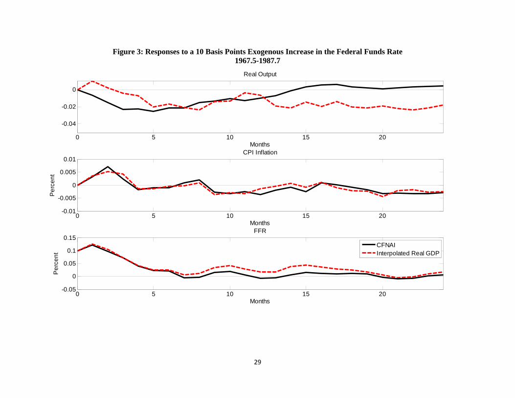
Figure 3 illustrates that the implications of our modified VAR model using the CFNAI
measure of real output are more economically plausible than those from the same model using
interpolated real GDP as in BGW. In particular, the latter model implies an implausibly
persistent decline in real output in response to a monetary policy tightening. The real output
measure based on interpolated and HP-filtered real GDP as in BGW’s analysis returns to its
steady state only after four years, compared with one and a half years if real output is measured
based on the CFNAI. The inflation and interest rate dynamics are very similar. We conclude that
our modified model provides a credible baseline for further analysis.
4.2. Systematic Policy Responses to an Oil Price Shock during 1967-1987
The main question of interest is how the Federal Reserve responds endogenously to an oil price
shock. We consider a 10 percent increase to the real price of oil not related to other innovations
in global commodity prices. Our initial analysis focuses on 1967.5-1987.7. The results in the left
column of Figure 4 are seemingly very much in line with the narrative in BGW. The oil price
shock is associated with a persistent increase in the real price of oil. Within two months, CPI
inflation sharply spikes. Following the spike in inflation, the federal funds rate rises temporarily,
followed by a temporary drop in real output and a gradual reduction in inflation. The decline in
the CFNAI reaches -0.5 after one year. Most past recessions have been associated with a value of
-0.7 or lower. Compared with the original BGW results, the interest rate response is somewhat

10
smaller. It only involves a cumulative increase within the first year of 60 basis points rather than
80 basis points. The magnitude of our estimate is consistent with Hamilton and Herrera’s (2004,
p. 282) preferred response estimate.
4.2.1. What Was the Federal Reserve Responding to?
It is useful to examine in more detail what variables the Federal Reserve is responding to in the
VAR model of section 4.1 by means of a decomposition of the policy response to the dynamics
triggered by an oil price shock. The intuition underlying this procedure is straightforward. In any
given period following an exogenous oil price shock, the deviation of the response of the federal
funds rate from the baseline of zero can be written as the sum of the response to its own lagged
values and of the responses to lagged values of other variables in the system. This allows us to
decompose which variables are driving the policy response.
Consider the structural VAR(p) representation
0 1 1 ... ,t t p t p tA y A y A y
where ty is the K -dimensional vector of variables, t denotes the vector of structural
innovations, the K K matrix 0A is lower triangular, and the intercept has been suppressed for
notational convenience. Express this VAR system as
1 1 ...t t t p t p ty Cy A y A y
where C is a K K dimensional lower triangular matrix with zeroes on the diagonal. Define
1 .pB C A A
The contribution of variable i to the response of the federal funds rate at horizon h to an oil price
shock at date 0 is given by:
min( , )
, , 5, ,2,0
0,1,2, ; 1,...., ,p h
FFR i h mK i i h mm
d B h i K
where ,2,i h m refers to the { ,2}i element of the K K impulse response coefficient matrix at
horizon ,h m denoted by h m , as defined in Lütkepohl (2005).
The left column of Figure 5 shows the decomposition of the response of the federal funds
rate in the left column of Figure 4 along these lines. To improve the readability of the graph,
results are shown in two separate plots. On impact, the response of the federal funds rate is
explained entirely by the Federal Reserve’s direct reaction to the oil price shock; there is

11
essentially no contemporaneous response to inflation, real output or commodity prices. For the
first three months, the Federal Reserve responds to the oil price shock by lowering interest rates,
which is inconsistent with the narrative of BGW. For the next three months, the Federal Reserve
responds directly to oil price shocks by raising the interest rate. There is little evidence of the
Federal Reserve’s policy response working through inflation. That response is negligible for the
first three months and small thereafter. The sign of the response to inflation varies across the
horizon. Likewise, there is very little reaction to the real output dynamics triggered by oil price
shocks. Thus, to a first approximation, almost all of the response of the federal funds rate after
the impact period is accounted for by the own lags of the federal funds rate.
This analysis is useful in that it shows that the Federal Reserve during the 1970s and
early 1980s responded not to actual inflation triggered by oil price shocks, but rather responded
directly to the oil price shocks, consistent with a preemptory move against potential inflationary
pressures. For example, the Federal Reserve might have been responding to oil price shocks
because they were seen as potential causes of wage-price spirals. This interpretation seems
conceivable in an unstable monetary environment. To the extent that this policy response is
successful in preempting the risk of inflation, one would never actually observe wage-price
spirals or a large response of inflation to the real price of oil in the data.
4.2.2. Counterfactual Analysis
The decomposition used in section 4.2.1 also is helpful in the construction of explicit
counterfactuals. The key contribution of BGW is the inclusion of the price of oil in the monetary
policy reaction function. How much of a difference does it make that the Federal Reserve is
allowed to respond directly to oil price shocks? The relevant counterfactual in answering this
question is not one in which the Federal Reserve holds the interest constant in response to an oil
price shock, as postulated by BGW, but a counterfactual in which the Federal Reserve reacts to
fluctuations in other macroeconomic state variables (such as inflation and real output) as it
normally would with only the direct response to the real price of oil being shut down. Below we
contrast the construction and implications of these two counterfactuals.
Under the counterfactual of only shutting down the direct response to the real price of oil,
we construct a sequence of hypothetical shocks to the federal funds rate that offsets the
contemporaneous and lagged effects of including the real price of oil in the policy reaction
function. This sequence of shocks is:

12
min( , )
, 5,2 2, 5, 2 2,1
, 0,1,2,...p h
FFR h h mK h mm
B x B z h
where ,0 , 1,..., ,ix i K denotes the contemporaneous response of variable i to the oil price shock
in the absence of a counterfactual policy intervention. The change in variable i in response to the
oil price shock after the counterfactual policy response is denoted by:
,0 ,0 ,5,0 ,0 5/ ,i i i FFRz x
where 5 denotes the standard deviation of the exogenous monetary policy shock. The
corresponding values for 0h can be generated recursively, starting with 1i from:
min( , )
, , , , ,1 1
p h K
i h i mK j i h m i j j hm j j i
x B z B x
and
, , ,5,0 , 5/ ,i h i h i FFR hz x
where 1,..., .j K
In contrast, for the original BGW counterfactual, which BGW refer to as the Sims-Zha
counterfactual based on a proposal in Sims and Zha (2006), one simply constructs a hypothetical
path of the shock ,FFR t that offsets all endogenous dynamics in the federal funds rate such that
the federal funds rate remains unchanged over time. In our notation, this can be expressed as: min( , )
, 5, ,5 5, ,1 1 1
, 0,1,2,...,p hK K
FFR h j j mK j j h mj m j
B x B z h
building on the same recursion as in the construction of the alternative counterfactual described
above. For an alternative description of the BGW counterfactual see Hamilton and Herrera
(2004).
Figure 6 compares these counterfactuals with the unconstrained responses in the VAR
model. Shutting down the direct response to oil price shocks has virtually no effect on inflation
and little effect on real output. The Federal Reserve still would have raised interest rates by a
roughly similar number of basis points in response to exogenous oil price shocks, but the bulk of
that response would have occurred three months later. This evidence casts serious doubt on the
narrative in BGW. For completeness we also include the original counterfactual computed as in
BGW in Figure 6. In that case, the federal funds rate remains constant by construction. This
policy would have had essentially no effect on inflation and real output would have been only

13
slightly higher, if at all.
An interesting question is what policy surprises each counterfactual would have involved
compared with actual policy choices. Figure 7 shows that under the new counterfactual interest
rates would have unexpectedly risen by about 17 basis points on impact, would have fallen by
about 33 basis points in month 4 after the oil price shock and would have risen again by about 25
basis points in month 6, relative to actual policy choices. This sequence of policy surprises is
somewhat different from that under the BGW counterfactual. One way of assessing how
reasonable the implied departures from actual policy outcomes would have been is to focus on
the magnitude of actual policy changes in the past; given that we are interested in unanticipated
policy changes, however, a better approach is to compare these implied changes to historical
policy shocks in the fitted VAR model. The largest policy surprises in the structural VAR model
are 446 and -662 basis points and occurred in 1980. About 30 percent of all policy shocks in the
sample period exceed 30 basis points and a further 32 percent are below -30 basis points. By that
standard, the policy changes of up to -33 basis points and up to +25 basis points required to
implement the counterfactuals in the left panel of Figure 7 do not seem unreasonable.
A closely related concern is that constructing any counterfactual is subject to the Lucas
critique (see Hamilton and Herrera 2004; Bernanke, Gertler and Watson 2004; Sims and Zha
2006). Rather than provide a comprehensive analysis of this issue, we follow Hamilton and
Herrera (2004) in analyzing BGW’s approach on its own terms. We follow the common
assumption in this literature of assuming that the policy changes contemplated are small enough
not to affect the structure of the economy materially. This assumption is more credible in our
context than in the original analysis in BGW because the counterfactuals in the left panel of
Figure 7 do not involve a surprise change in interest rates relative to actual policy outcomes in
the same direction “for 36 months in succession” (Hamilton and Herrera 2004, p. 269). The
obvious concern raised by Hamilton and Herrera is that the sequence of policy shocks required to
implement the counterfactual may be predictable. This is not a problem in the left panel of
Figure 7. It can be shown that not only is the sequence of policy shocks in Figure 7 required
under the new counterfactual less predictable than the sequence under the BGW counterfactual,
but that evaluating the first six autocorrelations of our policy shocks under the null of i.i.d.
shocks provides no evidence of statistically significant predictability. Moreover, the time path of
the federal funds rate shocks in the left panel of Figure 7 does not look noticeably different from

14
plots of actual policy surprises for a period of similar length in the estimated model. Hence, it is
not evidently unreasonable to presume that the model structure is stable with respect to these
policy interventions.
4.3. Does the Narrative Account in BGW Match Actual Policy Decisions?
Although our estimates for 1967-1987 – unlike the original estimates in BGW – pass simple
plausibility checks, as shown in the preceding section, there are other reasons to be skeptical of
BGW’s interpretation of the evidence. It is instructive to focus on the relationship of the
narrative account in BGW with the actual evolution of the federal funds rate during the two oil
price episodes of the 1970s. Although the Federal Reserve was not following an interest rate rule
at the time, we follow the literature in postulating that the federal funds rate effectively was
controlled by the Federal Reserve.11 The left panel of Figure 8 covers the first oil price shock
episode of late 1973 and early 1974. A striking feature of these data is that the Federal Reserve
had been raising interest rates steadily from early 1972 until mid-1973. This finding is consistent
with evidence from Federal Reserve policy statements. The Federal Reserve by its own account
was responding to rising commodity prices when it continuously raised interest rates long before
the oil price shock of late 1973. The observed rapid increases in global industrial commodity
prices in 1972/73 were an indication of an overheating global economy, consistent with the
analysis in Barsky and Kilian (2002). In contrast, when the oil price shocks did occur in late
1973, the Federal Reserve lowered interest rates for the first time in more than a year, consistent
with the interpretation of oil price shocks as adverse aggregate demand shocks. The decline in
interest rates continued into 1974, even after oil prices doubled again in January. Only in March
of 1974, interest rates began to rise again, reaching a peak in July, before gradually receding to
about 6 percentage points by early 1975.
This response is clearly different from the narrative account in BGW of a generic oil
price shock episode and BGW readily conceded that “the 1974-75 decline in real output is
generally not well explained by the oil price shock. The … major culprit was (non-oil)
commodity prices. Commodity prices … rose very sharply before this recession and stimulated a
sharp monetary policy response of their own.” (p. 121). Thus, BGW’s evidence in favor of a
monetary policy response to oil price shocks rests squarely on the 1979 episode covered in the
11 For related accounts of U.S. monetary policy in the 1970s see Barsky and Kilian (2002) and Kozicki and Tinsley (2009).

15
right panel of Figure 8. Given that both the federal funds rate and the real price of oil began to
increase in May of 1979, it is not surprising that data from this episode tend to dominate
estimates of the contemporaneous correlation of oil price shocks and interest rate changes.12 This
fact is troublesome because we do not know whether Paul Volcker raised interest rates in
response to the oil price shock of 1979 or in response to rising inflation driven by domestic
policies. Given that both interest rates and oil prices moved at about the same time, it is difficult
to separate correlation from causation. In short, there is reason to suspect an identification
problem. This explanation also would help account for the fact that the interest rate response to
oil price shocks does not work through the higher inflation or lower output triggered by
unexpected oil price increases, but rather occurs in direct response to the real oil price increase,
as we documented earlier (see left panel of Figure 5). This is precisely the type of pattern we
would expect if the VAR model incorrectly interpreted an exogenous increase in interest rates
under Chairman Volcker as an endogenous response to the oil price shocks of 1979.
4.4. Systematic Policy Responses to an Oil Price Shock during 1987-2008
The discussion in section 4.3 suggests that the monetary policy response to oil price shocks is not
well identified. Much depends on whether we interpret the rise in interest rates in 1979 under
Paul Volcker as a response to the oil price shocks of that year or as a shift in the policy regime
away from the employment objective that would have taken place even in the absence of the oil
price shocks of 1979. One way of discriminating between these hypotheses is to focus on the
pre-Volcker period 1967.5-1979.7. Estimates for this period (which are not shown to conserve
space) indicate that in response to an oil price shock the Federal fund rate initially declines below
its mean, then rises substantially above its mean (with a peak after 7 months), and finally drops
substantially below its mean (with a trough after 17 months), before returning to its mean. This
pattern roughly matches the evolution of the federal funds rate after late 1973 in the left panel of
Figure 8. The estimated responses of the federal funds rate are statistically significant based on
one-standard error bands. Clearly, this response pattern differs from the narrative in BGW who
did not envision that the Federal Reserve would lower the interest rate in response to an oil price
shock in the short run or, for that matter, in the second year following the oil price shock. These
12 BGW (p. 133) are aware of this point. They acknowledge the instability of their VAR results across subsamples, but attribute the stronger response of the Federal Reserve to oil price shocks during 1976-85 to the Federal Reserve’s substantially increased concern with inflation during the Volcker era.

16
estimates are not dispositive, however, because there is reason to doubt that the Federal Reserve
prior to Paul Volcker was committed to the price stability objective.
We also estimated the same model for the Volcker period of 1979.8-1987.7 for
comparison (with pre-sample observations from the pre-Volcker period). Interestingly, the
estimated responses provide no support for the notion that Volcker raised interest rates in
response to oil price shocks and thereby caused a recession, although we hasten to add that this
sample is likely to be too small to allow meaningful inference. A better way of assessing whether
there is an identification problem in 1979 is to focus on the post-Volcker period. Clearly,
Greenspan and Bernanke have been rightly credited for putting the inflation objective first in the
tradition of Volcker’s policies, and there have been enough oil price shocks between 1987 and
2008 to help us identify the Federal Reserve’s systematic policy response to oil price shocks.
The right column of Figure 4 shows that there is no evidence at all of systematic
monetary policy responses to oil price shocks after 1987, during the Greenspan-Bernanke era.
Although the response of the real price of oil to an oil price shock is quite similar to that in the
first subsample, there is almost no increase in the federal funds rate or in real output and the path
of inflation shows no evidence of significant price pass-through even in the absence of a policy
reaction. Only on impact and twelve months later are there small spikes in inflation. The right
column in Figure 5 decomposes the rather small response of the federal funds rate further. The
positive impact response reflects a direct response to the oil price shock; subsequent federal
funds rate movements are merely responses to own lags. Finally, the right column in Figure 6
illustrates that the counterfactual departures from the actual policy outcomes would have made
essentially no difference for the inflation and real output responses. In light of that finding, the
implication of Figure 7 (right column) that the original BGW counterfactual (unlike the
alternative counterfactual proposed in this paper) would have involved positive policy surprises
for at least three years in a row, which hardly seems plausible, is a moot point. On the basis of
these results, there clearly is no reason to include the real price of oil in the policy reaction
function of the VAR model after 1987.
5. Historical Decompositions
An alternative explanation of the lack of evidence of a monetary policy response after 1987 is
that oil price shocks have become less inflationary over time, allowing the policymaker to

17
respond less aggressively to oil price shocks without causing a major recession.13 The implicit
premise in this literature is that monetary policy responses to oil price shocks had large
cumulative effects on real activity prior to 1987, making it important to explain the absence of
large cumulative effects after 1987. Large responses to a one-time oil price shock, however, need
not translate into large cumulative effects of oil price shocks on macroeconomic aggregates in
actual data because the actual data involve a vector sequence of oil price innovations of different
magnitudes and signs. Thus, in assessing the historical evidence, we need to move beyond
impulse response analysis and construct historical decompositions of the data. Figure 9 shows
that, notwithstanding the impulse response results in Figure 4, the cumulative contribution of oil
price shocks through time on U.S. real output in particular is negligible. Figure 9 plots the actual
(demeaned) real output and inflation data and the fluctuations in the same variable explained by
the direct effect of oil price shocks and the endogenous policy response combined. It is evident
that oil price shocks overall had little impact on observed U.S. real activity and inflation even in
the first subsample. Likewise, we see that oil price shocks had little effect on the federal funds
rate not only in 1973/74, but more importantly under Volcker in 1979/80.
Because the indirect effect on U.S. real activity associated with the monetary policy
response and the direct effect of oil price shocks on U.S. real activity are of the same sign, an
immediate implication of Figure 9 is that central bankers’ monetary policy responses to oil price
shocks cannot have been a major contributor to the U.S. recessions of the 1970s and the early
1980s.14 This result is quite powerful in that it does not depend on any counterfactual and is in
striking contrast to BGW’s original analysis.
Despite BGW’s failure to explain the 1974/75 recession based on the Federal Reserve’s
reaction to the oil price shock and despite their limited success in explaining subsequent
recessions based on policy reactions to oil price shocks, BGW concluded that the data overall
were supportive of a dominant role for monetary policy reactions. The historical decomposition
of real output in Figure 9 does not support that view. There is no indication that U.S. real
activity would have been much different under alternative policy scenarios, even in the late
1970s and early 1980s, despite the fact that our results pass standard tests of whether the
13 For related discussion see Blanchard and Galí (2010), Herrera and Pesavento (2009), Edelstein and Kilian (2009), and Kilian (2009, 2010), among others. 14 A very similar result applies to the second subsample (but is not shown to conserve space). The model provides no evidence that a monetary policy response to oil price shocks played a dominant role in the recessions of 1990, 2001, or late 2007, for example.

18
counterfactual is reasonable, as discussed in section 4.2.2. This conclusion is much more in line
with the theoretical results in Carlstrom and Fuerst (2006) of the impotence of systematic
monetary policy than with BGW’s original results, although unlike Carlstrom and Fuerst we do
not find any evidence of large direct effects of oil price shocks on the U.S. economy either.
It is interesting to compare our findings to the analysis in Herrera and Pesavento (2009).
As part of a comprehensive study of potential causes of the Great Moderation, Herrera and
Pesavento (2009) examined the extent to which systematic monetary policy responses had
dampened fluctuations in real activity during the 1970s. Unlike our model, theirs was based on
quarterly data. Here we consider a simplified version of their model. Figure 10 presents historical
decompositions for quarterly U.S. real GDP growth and GDP deflator inflation. The recursively
identified model includes the percent change in the real price of oil, the percent growth rate of
real GDP, GDP deflator inflation and the federal funds rate (in that order).15 The results shown
are based on the same sample period of 1967.II-1987.II. Essentially identical results would be
obtained using Herrera and Pesavento’s original sample period. Figure 10 contrasts the actual
demeaned data with the cumulative effect of oil price shocks on real GDP growth and deflator
inflation. Notwithstanding important differences in the sample period, model specification and
data, the empirical results are fully consistent with our earlier analysis. In particular, the
historical decompositions of real GDP growth based on the quarterly model in Figure 10
substantively agree with our historical decompositions of the CFNAI measure of real output in
Figure 9. Regardless of the model adopted, there is no evidence that oil price shocks indirectly
through the monetary policy reaction or directly were a major contributor to the recessions of
1974/75, 1980 or 1981-83.
6. Toward a New Class of Monetary Policy Reaction Functions
One reason why the conventional monetary policy reaction model fails to explain large
fluctuations in U.S. real activity may be that not all oil price shocks are the same. Oil price
shocks are best viewed as symptoms of deeper structural shocks in oil markets. One would
expect the Federal Reserve to respond differently to oil price shocks associated with, say,
15 We follow Herrera and Pesavento in fitting a VAR(4) model. Unlike Herrera and Pesavento we order the percent change in the real price of oil first in line with the results in Kilian and Vega (2009) and we drop the growth rate of potential output. These changes do not materially alter the results of the historical decomposition nor does the exclusion of industry level variables that do not relate to our analysis. Our results for real GDP growth are substantively identical with those in Herrera and Pesavento (2009, Figure 7) for the larger quarterly model.

19
unexpected booms in global demand, than oil supply disruptions. An unexpected demand boom
driven by the global business cycle, for example, will stimulate the U.S. economy in the short
run, whereas an unanticipated oil supply disruption will not, calling for different policy
responses depending on the composition of the oil demand and oil supply shocks underlying the
oil price shock. For that reason one would not expect the relationship between interest rates and
the real price of oil to be stable over time.16
Figure 11 investigates this point by adding the federal funds rate as the fourth variable to
the recursively identified VAR model utilized in Kilian (2009).17 We trace out the effects on the
federal funds rate of unanticipated oil supply disruptions (“oil supply shocks”), unexpected
positive innovations to the global business cycle (“aggregate demand shocks”) and demand
shocks that are specific to the oil market (“oil-market specific demand shocks”). Figure 11
shows that the Federal Reserve tends to respond to positive oil demand shocks by raising the
interest rate, whereas it tends to lower the interest rate in response to oil supply disruptions. The
positive response to aggregate demand shocks in particular is consistent with the Federal
Reserve’s decision to raise interest rates long before the oil price shock of late 1973. The
negative response to unanticipated oil supply disruptions is consistent with the view that the
Federal Reserve views the resulting oil price increases as adverse aggregate demand shocks.
Interpreting the positive response to demand shocks in this context is more difficult, as higher oil
prices are but one of many consequences of such demand shocks.
Although the responses shown in Figure 11 correctly represent historical averages, they
need not be representative of actual policy responses at any given point in time. Even granting
that the Federal Reserve does distinguish between oil demand and oil supply shocks in setting
interest rates, it would be surprising if the Federal Reserve had pursued a consistent policy over
time. It is equally important to recognize that embedding such a modified policy reaction
function in the BGW model and estimating this VAR model on historical data is not a sensible
idea. On the one hand, the well-documented shifts in U.S. monetary policy regimes between
1973 and 2008 imply that any VAR model that embeds oil demand and supply shocks in the
policy reaction function would have to allow for time-varying coefficients or would have to be
16 Note that this source of instability is different from the other potential explanations in that it does not involve changes in the unconditional distribution of the economy. 17 The assumption that the price of oil and hence that oil demand and supply shocks are predetermined with respect to the U.S. interest rate is consistent with evidence in Kilian and Vega (2010).

20
based on split samples. On the other hand, the methodology underlying Figure 11 requires long
samples with sufficient variation in all oil demand and oil supply shocks to ensure identification.
Thus, the idea of embedding oil demand and oil supply shocks within a time-varying parameter
VAR monetary policy reaction function, while perhaps natural, does not seem practical.
This caveat does not apply, however, to theoretical studies of the optimal monetary
policy response to oil demand and oil supply shocks. Such studies require a different class of
structural models than are customarily used by policy makers and macroeconomists.
Recent advances in the DSGE modeling of endogenous oil price shocks are a step in that
direction.18 While none of these papers provides a comprehensive analysis of all relevant aspects
of the relationship between oil prices and the macro economy, a new class of models is
beginning to emerge that allows policymakers to respond differently to different types of oil
price shocks.19 Such DSGE models also will allow economists to distinguish between alternative
causes of fluctuations in the global demand for industrial commodities, and to simulate the
impact of alternative policy choices. Given that traditional DSGE models of the role of
systematic monetary policy responses to oil price shocks ignore the distinction between different
oil demand and oil supply shocks, they are not directly relevant to question of how the Federal
Reserve should respond to shocks in global oil markets. Thus, the fundamental question raised in
BGW of how large the effects are of systematic monetary policy responses to these shocks
remains as relevant as ever.
7. Conclusion
Since BGW (1997), a common view in the literature has been that systematic monetary policy
responses to the actual or potential inflationary pressures triggered by oil price shocks are an
important source of aggregate fluctuations in the U.S. economy. Notwithstanding the popularity
of this view, doubts remain about the empirical strategy used in support of that proposition.
Using improved model specifications, additional data, and additional econometric tools that aid
in the interpretation of the model estimates, we documented that there is no empirical support for
an important role of monetary policy responses in amplifying the effects of oil price shocks.
18 For example, Bodenstein, Erceg and Guerrieri (2007) model oil-market specific demand shocks, and Balke, Brown, and Yücel (2009) model the dependence of oil demand on global macroeconomic conditions. In related work, Nakov and Pescatori (2010) explicitly model the endogeneity of oil production decisions. 19 Useful extensions in this context also include a model of the external transmission of oil demand and oil supply shocks (see Kilian, Rebucci and Spatafora 2009) and of the nexus between crude oil prices and retail energy prices (see Edelstein and Kilian 2009).

21
This finding is not completely surprising. We observed that the narrative underlying BGW’s
analysis of the 1970s is not self-evident in light of economic theory and at odds with recent
empirical and theoretical work accounting for the endogeneity of the price of oil. Moreover,
actual policy actions during the two oil price shock episodes of the 1970s do not fit well with the
narrative account in BGW.
It is useful to put our results in perspective relative to earlier studies of the BGW model.
Hamilton and Herrera (2004) aimed to show that the monetary policy response to oil price
shocks in BGW’s model was implausibly large. They made the case that the counterfactual
constructed in BGW was not credible because it evidently violated the Lucas critique. Based on
our analysis of the same sample period, using the same criteria employed in Hamilton and
Herrera, the economically more relevant counterfactual proposed in this paper of shutting down
the response to oil price shocks appears credible. Nevertheless, there is no evidence that the
monetary policy response had large effects on U.S. real activity or CPI inflation. The latter
conclusion is independent of the choice of counterfactual. Hence, our results differ from BGW’s,
but for different reasons than Hamilton and Herrera’s.
Hamilton and Herrera (2004) also made the case that the direct effects of oil price shocks
on the U.S. economy were substantial, making it less important to consider mechanisms of
amplifying the effects of oil price shocks such as endogenous monetary policy responses.
In contrast, we found that the combined direct and indirect effect of oil price shocks on the U.S.
economy has been negligible. This result is driven mainly by the specification of the oil price
shock measure. The censored VAR model used in BGW’s and in Hamilton and Herrera’s (2004)
analysis has been shown to yield inconsistent impulse response estimates (see Kilian and
Vigfusson 2009). Indeed, such inconsistent models tend to show much larger effects of oil price
shocks on real output than the estimates we found. Given the lack of evidence for asymmetries in
the responses of real output to oil price innovations recently documented in Kilian and
Vigfusson, our analysis relies on conventional linear VAR specifications rather than alternative
nonlinear regression models. Such models are consistent with standard macroeconomic models
of the transmission of oil price shocks and can be consistently estimated using standard methods.
A potential concern with all monetary policy VAR models is the possibility of breaks in
the policy reaction function associated with the transition from one chairman of the Federal
Reserve to the next. Our subsample analysis addressed this issue within the constraints imposed

22
by the data. In addition to reexamining the analysis of BGW on data for the 1967.5-1987.7
period (as well as the Volcker and pre-Volcker era within that period), we examined in detail
policy responses to oil price shocks during the Greenspan-Bernanke era of 1987.8-2008.6. Ours
is not the first study to find important differences in policy responses after 1987. For example, as
part of a comprehensive study of potential causes of the Great Moderation, Herrera and
Pesavento (2009) concluded that systematic monetary policy responses had dampened
fluctuations in real activity during the 1970s, but had virtually no effect after the mid-1980s.
Their conclusion appears to have been based on impulse response analysis and forecast error
variance decompositions. Indeed, notwithstanding important differences in the sample period,
model specification and data, our empirical analysis supported their conclusions, as far as
impulse response analysis is concerned. The difference is in the emphasis. Whereas Herrera and
Pesavento (2009) stressed differences in average volatility and in the magnitude of impulse
responses across the two samples, we are more specifically concerned with the ability of
systematic monetary policy responses to explain specific recessions in the 1970s and early
1980s. We showed that, even before the mid-1980s, systematic monetary policy responses were
not a dominant source of the real effects of oil price shocks. Our analysis showed that historical
decompositions of real GDP growth based on Herrera and Pesavento’s quarterly model
substantively agree with our historical decompositions of the CFNAI measure of monthly real
output. Regardless of the model adopted, there is no evidence that oil price shocks indirectly
through the monetary policy reaction or directly were a major contributor to the recessions of
1974/75, 1980 or 1981-83.
An important question in the recent literature has been what explains the apparent
absence of a monetary policy response after the mid-1980s. We stressed that the evidence in
favor of policy responses to oil price shocks in the 1970s and early 1980s is heavily influenced
by the episode of 1979, and that it is unclear whether Volcker raised interest rates in 1979 in
response to the oil price shock or whether he would have raised interest rates in response to
rising inflation even in the absence of that shock. To the extent that there is no causal link from
the oil price shock of 1979 to rising interest rates, the disappearance of this dynamic correlation
in subsequent data is not surprising.
Much of the discussion in this paper has been about whether there were large real effects
from monetary policy responses to oil price shocks in the 1970s and early 1980s. It may seem

23
that this question should be primarily of interest to economic historians. This interpretation
would be a mistake. Not only is this question central in designing theoretical models of the
transmission of oil price shocks, but recent work by Harris et al. (2009), for example, has
suggested that the Federal Reserve after 2005 may have been too passive in dealing with the
determinants of high asset and oil prices. The question of how to respond to higher oil prices is
likely to take on a new urgency, as the world economy recovers from the current crisis.
Moreover, the policy environment of 2009 in many ways resembles that at the beginning of the
1970s (see Kilian 2010). Understanding the monetary policy regimes in that era, to what extent
they were successful, and to what extent they can be improved upon is crucial for monetary
policy makers as the global recovery unfolds.
Our analysis suggests that the traditional monetary policy reaction framework explored
by BGW and incorporated in subsequent DSGE models has outlived its usefulness. There is
growing, but not yet universal, awareness that it would be a mistake for policy makers to respond
to oil price shocks rather than its underlying determinants. Rather than respond to relative price
shocks that often are merely symptoms of broader global macroeconomic developments, central
banks must identify and respond to the deeper causes of oil price shocks. This requires a
different class of structural models than are customarily used by policy makers. It calls for DSGE
models that take account of the endogeneity of the real price of oil and that allow policy
responses to depend on the underlying causes of oil price shocks. Recent advances in the DSGE
modeling of oil price shocks have made important strides in that direction, although more
remains to be done to make these models operational for policy use.

24
References
Angelini, E., Henry, J., and M. Marcellino (2006), “Interpolation and Backdating with a Large Information Set,” Journal of Economic Dynamics and Control, 30, 2693-2724.
Balke, N.S., S.P.A. Brown, and M.K. Yücel (2009), “Oil Price Shocks and U.S. Economic Activity: An International Perspective,” mimeo, Federal Reserve Bank of Dallas. Bańbura, M., Giannone, D., and L. Reichlin (2008), “Bayesian VARs with Large Panels,” Journal of Applied Econometrics, 25, 71-92. Barsky, R.B., and L. Kilian (2002), “Do We Really Know that Oil Caused the Great Stagflation? A Monetary Alternative,” in: NBER Macroeconomics Annual 2001, B.S. Bernanke and K. Rogoff (eds.), MIT Press: Cambridge, MA, 137-183. Barsky, R.B., and L. Kilian (2004), “Oil and the Macroeconomy Since the 1970s,” Journal of Economic Perspectives, 18(4), 115-134. Bernanke, B.S., Boivin, J., and P. Eliasz (2005), “Measuring the Effects of Monetary Policy: A
Factor Augmented Vector Autoregressive (FAVAR) Approach,” Quarterly Journal of Economics, 120, 387-422.
Bernanke, B.S., Gertler, M., and M.W. Watson (1997), “Systematic Monetary Policy and the Effects of Oil Price Shocks,” Brookings Papers on Economic Activity, 1, 91-157. Bernanke, B.S., Gertler, M., and M.W. Watson (2004), “Reply to Oil Shocks and Aggregate Economic Behavior: The Role of Monetary Policy,” Journal of Money, Credit and Banking, 36, 287-291. Blanchard, O.J., and J. Galí (2010), “The Macroeconomic Effects of Oil Shocks: Why are the 2000s so Different from the 1970s?” Forthcoming in: J. Galí and M. Gertler (eds.), International Dimensions of Monetary Policy, University of Chicago Press: Chicago, IL. Bodenstein, M., Erceg, C.J., and L. Guerrieri (2007), “Oil Shocks and U.S. External
Adjustment,” mimeo, Federal Reserve Board. Carlstrom, C.T., and T.S. Fuerst (2006), “Oil Prices, Monetary Policy, and Counterfactual Experiments,” Journal of Money, Credit and Banking, 38, 1945-1958. Christiano, L.J., Eichenbaum, M., and C.L. Evans (1999), “Monetary Policy Shocks: What Have We Learned and to What End?” Handbook of Macroeconomics, 1, Chapter 2, Elsevier Science, 65-148. Edelstein, P., and L. Kilian (2009), “How Sensitive are Consumer Expenditures to Retail Energy Prices?” Journal of Monetary Economics, 56, 766-779.

25
Evans, C.L. (1999), “If You Were the Central Banker, How Many Data Series Would You Watch? An Empirical Analysis.” mimeo, Federal Reserve Bank of Chicago. Gonçalves, S., and L. Kilian. (2004), “Bootstrapping Autoregressions with Conditional Heteroskedasticity of Unknown Form,” Journal of Econometrics, 123(1), 89-120. Hamilton, J. D. (1996). “This is What Happened to the Oil Price–Macroeconomy Relationship,”
Journal of Monetary Economics, 38, 215–220. Hamilton, J. D. (2003) “What is an Oil Shock?” Journal of Econometrics, 113, 363–398. Hamilton, J.D., and A.M. Herrera (2004), “Oil Shocks and Aggregate Economic Behavior: The Role of Monetary Policy,” Journal of Money, Credit and Banking, 36, 265-286. Harris, E.S., Kasman, B.C., Shapiro, M.D., and K.D. West (2009), “Oil and the Macroeconomy:
Lessons for Monetary Policy,” mimeo, University of Wisconsin. Herrera, A.M., and E. Pesavento (2009), “Oil Price Shocks, Systematic Monetary Policy, and the
‘Great Moderation’,” Macroeconomic Dynamics, 13, 107-137. Kilian, L. (2008a), “The Economic Effects of Energy Price Shocks,” Journal of Economic Literature, 46(4), 871-909. Kilian, L. (2008b), “A Comparison of the Effects of Exogenous Oil Supply Shocks on Output and Inflation in the G7 Countries,” Journal of the European Economic Association, 6, 78-121. Kilian, L. (2009), “Not All Oil Price Shocks Are Alike: Disentangling Demand and Supply Shocks in the Crude Oil Market,” American Economic Review, 99(3), 1053-1069. Kilian, L. (2010), “Oil Price Shocks, Monetary Policy and Stagflation,” forthcoming in: Fry, R., Jones, C., and C. Kent (eds.), Inflation in an Era of Relative Price Shocks, Sydney, 2010. Kilian, L., A. Rebucci and N. Spatafora (2009), “Oil Shocks and External Balances,” Journal of International Economics, 77, 181-194. Kilian, L., and C. Vega (2010), “Do Energy Prices Respond to U.S. Macroeconomic News? A
Test of the Hypothesis of Predetermined Energy Prices,” forthcoming: Review of Economics and Statistics.
Kilian, L., and R. Vigfusson (2009), “Are the Responses of the U.S. Economy Asymmetric in Energy Price Increases and Decreases?” mimeo, Department of Economics, University of Michigan. Kozicki, S., and P.A. Tinsley (2009), “Perhaps the 1970s’ FOMC Did What It Said It Did?” Journal of Monetary Economics, 56, 842-855.

26
Leduc, S., and K. Sill (2004), “A Quantitative Analysis of Oil Price Shocks, Systematic
Monetary Policy, and Economic Downturns,” Journal of Monetary Economics, 51, 781- 808.
Lütkepohl, H. (2005), New Introduction to Multiple Time Series Analysis, Springer: Berlin. Mork, K.A. (1989), “Oil and the Macroeconomy. When Prices Go Up and Down: An Extension of Hamilton’s Results,” Journal of Political Economy, 97, 740‐744. Nakov, A., and A. Pescatori (2010), “Monetary Policy Trade-Offs with a Dominant Oil Producer,” Journal of Money, Credit, and Banking, 42, 1-32. Rotemberg, J. (2010), “Comment on Blanchard-Gali: The Macroeconomic Effects of Oil Price Shocks: Why are the 2000s so different from the 1970's?” Forthcoming in: J. Galí and M. Gertler (eds.), International Dimensions of Monetary Policy, University of Chicago
Press: Chicago, IL. Rotemberg, J., and M. Woodford (1996), “Imperfect Competition and the Effects of Energy Price Increases on Economic Activity,” Journal of Money, Credit, and Banking, 28, 550- 77. Sims, C.A., and T. Zha (2006), “Does Monetary Policy Generate Recessions?” Macroeconomic
Dynamics, 10, 231-272. Stock, J.H., and M.W. Watson (1999), “Forecasting Inflation,” Journal of Monetary Economics, 44, 293-335.

27
1970 1975 1980 1985 1990 1995 2000 2005-5
-4
-3
-2
-1
0
1
2
3
4
5CFNAI versus Percent Deviations of Quarterly Real GDP from HP-Trend
CFNAIGDP
Figure 1: Alternative Measures of the Business Cycle in U.S. Real Output
Notes: Three-month moving average of the Chicago Fed National Activity Index (CFNAI) and HP-filtered log real U.S. GDP in percent deviation from trend. NBER recessions are shown as shaded areas.

28
0 5 10 15 20-0.5
0
0.5Real Price of Commodities
Per
cent
0 5 10 15 20-0.5
0
0.5Real Price of Oil
Per
cent
0 5 10 15 20-0.04
-0.02
0
0.02CFNAI
Inde
x
0 5 10 15 20-0.01
0
0.01
0.02CPI Inflation
Per
cent
0 5 10 15 20-0.1
0
0.1
0.2FFR
Per
cent
Months0 5 10 15 20
-0.06
-0.04
-0.02
0
0.02CPI
Per
cent
Months
Figure 2: Responses to a 10 Basis Points Exogenous Increase in the Federal Funds Rate (with 1-Standard Error Bands) 1967.5-1987.7
Notes: The error bands were constructed using the recursive-design wild bootstrap method of Goncalves and Kilian (2004).
29
0 5 10 15 20
-0.04
-0.02
0
Months
Real Output
0 5 10 15 20-0.01
-0.005
0
0.005
0.01CPI Inflation
Months
Per
cent
0 5 10 15 20-0.05
0
0.05
0.1
0.15FFR
Months
Per
cent
CFNAIInterpolated Real GDP
Figure 3: Responses to a 10 Basis Points Exogenous Increase in the Federal Funds Rate 1967.5-1987.7

30
0 5 10 15 200
20
40Real Price of Oil
Per
cent
0 5 10 15 200
20
40Real Price of Oil
Per
cent
0 5 10 15 20
-0.5
0
0.5CFNAI
Inde
x
0 5 10 15 20
-0.5
0
0.5CFNAI
Inde
x
0 5 10 15 20
-0.2
0
0.2
CPI Inflation
Per
cent
0 5 10 15 20
-0.2
0
0.2
CPI Inflation
Per
cent
0 5 10 15 20-1
0
1
FFR
Per
cent
Months0 5 10 15 20
-1
0
1
FFR
Per
cent
Months
Figure 4: U.S. Responses to a 10 Percent Real Oil Price Shock (with One-Standard Error Bands)
1967.5-1987.7 1987.8-2008.6
Notes: Estimates based on recursively identified VAR(12) model for the percent change in real CRB commodity prices, the percent change in the real price of oil, CFNAI, CPI inflation and the federal funds rate. A CFNAI value below -0.7 is commonly associated with the onset of a recession (see http://www.chicagofed.org/digital_assets/publications/cfnai/background/cfnai_background.pdf).

31
0 5 10 15 20-0.5
0
0.5
1
Per
cent
1967.5 - 1987.7
0 5 10 15 20-0.5
0
0.5
1
Months
Per
cent
0 5 10 15 20-0.5
0
0.5
1
Per
cent
1987.8 - 2008.6
Total FFRReal Commodities PriceReal Oil PriceFFR
0 5 10 15 20-0.5
0
0.5
1
Months
Per
cent
Total FFRCFNAICPI Inflation
Figure 5: Decomposition of the Response of the Federal Funds Rate to a 10 Percent Real Oil Price Shock
Notes: The decomposition underlying this figure is described in section 4.2.1.

32
0 5 10 15 20
-0.4
-0.2
0
0.2
CFNAI
Inde
x
0 5 10 15 20
-0.4
-0.2
0
0.2
CFNAI
Inde
x
0 5 10 15 20
-0.2-0.1
00.10.2
CPI Inflation
Per
cent
0 5 10 15 20
-0.2-0.1
00.10.2
CPI Inflation
Per
cent
0 5 10 15 20-1
-0.5
0
0.5
1FFR
Per
cent
0 5 10 15 20-1
-0.5
0
0.5
1FFR
Per
cent
Unrestricted BGW Counterfactual New Counterfactual
Figure 6: Counterfactual Simulations
1967.5-1987.7 1987.8-2008.6
Notes: BGW Counterfactual refers to the counterfactual of holding constant the interest; New Counterfactual refers to the counterfactual of shutting down the direct monetary policy response to oil price shocks in the policy reaction function.

33
10 20 30 40 50-40
-30
-20
-10
0
10
20
30
Bas
is P
oint
s
Months
1967.5 - 1987.7
New CounterfactualBGW Counterfactual
10 20 30 40 50-5
-4
-3
-2
-1
0
1
2
3
4
5
Bas
is P
oint
s
Months
1987.8 - 2008.6
Figure 7: Policy Shocks Required for the Implementation of the Counterfactual
Notes: BGW Counterfactual refers to the counterfactual of holding constant the interest; New Counterfactual refers to the counterfactual of shutting down the direct monetary policy response to oil price shocks in the policy reaction function.

34
1972.5 1973 1973.5 1974 1974.5 1975 1975.5 19760
2
4
6
8
10
12
January 1974
October 1973
1979.5 1980 1980.5 1981 1981.5 1982 1982.5 1983 1983.5 19840
2
4
6
8
10
12
14
16
18
20
April 1979
February 1981
Figure 8: The Evolution of the Federal Funds Rate during the Oil Price Shocks of the 1970s and Early 1980s
Notes: In October of 1973 and January of 1974 the price of oil doubled. April 1979 marks the beginning of the 1979 oil price surge; in February of 1981 the price of imported crude oil peaks.

35
1972 1974 1976-6
-4
-2
0
2
Inde
xCFNAI
1972 1974 1976-1
-0.5
0
0.5
1
1.5
2
Per
cent
CPI Inflation
1972 1974 1976-6
-4
-2
0
2
4
6
Per
cent
FFR
1979 1981 1983-4
-3
-2
-1
0
1
2
Inde
x
CFNAI
1979 1981 1983-1
-0.5
0
0.5
1
1.5
2P
erce
ntCPI Inflation
1979 1981 1983-5
0
5
10
15
Per
cent
FFR
Demeaned Actual Cumulative Effect
Figure 9: Cumulative Effect of Real Oil Price Shocks on U.S. Real Output, Inflation and Interest Rates: Selected Episodes Monthly Baseline Model
Notes: Historical decompositions constructed from the monthly model underlying Figure 4.

36
1972 1972.5 1973 1973.5 1974 1974.5 1975 1975.5 1976 1976.5 1977-4
-3
-2
-1
0
1
2
3
4Real GDP Growth
Per
cent
Cumulative EffectDemeaned Actual
1972 1972.5 1973 1973.5 1974 1974.5 1975 1975.5 1976 1976.5 1977-2
-1.5
-1
-0.5
0
0.5
1
1.5
2GDP Deflator Inflation
Per
cent
1979 1979.5 1980 1980.5 1981 1981.5 1982 1982.5 1983 1983.5 1984-4
-3
-2
-1
0
1
2
3
4Real GDP Growth
Per
cent
1979 1979.5 1980 1980.5 1981 1981.5 1982 1982.5 1983 1983.5 1984-2
-1.5
-1
-0.5
0
0.5
1
1.5
2GDP Deflator Inflation
Per
cent
Figure 10: Cumulative Effect of Real Oil Price Shocks on U.S. Real Output and Inflation: Selected Episodes Quarterly Model
Notes: Estimates based on macroeconomic block and oil block of the quarterly VAR model of Herrera and Pesavento (2009). Unlike Herrera and Pesavento we order the percent change in the real price of oil first in line with the results in Kilian and Vega (2009) and we drop the growth rate of potential output. These changes do not materially alter the results. The results shown are based on the same sample period as our earlier estimates. Essentially identical results for the upper row would be obtained using Herrera and Pesavento’s original sample period.

37
0 5 10 15-0.4
-0.3
-0.2
-0.1
0
0.1
0.2
0.3
0.4
0.5Oil supply shock
Per
cent
Months0 5 10 15
-0.4
-0.3
-0.2
-0.1
0
0.1
0.2
0.3
0.4
0.5Aggregate demand shock
Per
cent
Months0 5 10 15
-0.4
-0.3
-0.2
-0.1
0
0.1
0.2
0.3
0.4
0.5Oil-specific demand shock
Per
cent
Months
Figure 11: Response of the Effective Federal Funds Rate to Oil Demand and Oil Supply Shocks (with One-Standard Error Bands)
Notes: Estimates from a recursively identified oil-market VAR model based on Kilian (2009) augmented by the change in the federal funds rate as the fourth variable. The sample period is 1973.2-2008.6. All shocks have been normalized to imply an increase in the real price of oil. Aggregate demand shocks refer to shocks that increase global demand for all industrial commodities (including crude oil); oil-specific demand shocks are other shocks that increase the demand for crude oil; oil supply shocks represent unexpected disruptions of the global production of crude oil.