University of Nebraska - LincolnDigitalCommons@University of Nebraska - Lincoln

Library Philosophy and Practice (e-journal) Libraries at University of Nebraska-Lincoln

2012

Does the Digital Environment Improve ModernUsers' Internet Awareness?T SaravananAnnamalai University, sarlib@live.in

M. M. KalaivaniAnnamalai University

V. SenthilkumarAnnamalai University

Follow this and additional works at: http://digitalcommons.unl.edu/libphilprac

Part of the Library and Information Science Commons

Saravanan, T; Kalaivani, M. M.; and Senthilkumar, V., "Does the Digital Environment Improve Modern Users' Internet Awareness?"(2012). Library Philosophy and Practice (e-journal). 773.http://digitalcommons.unl.edu/libphilprac/773

http://unllib.unl.edu/LPP/

Library Philosophy and Practice 2012

ISSN 1522-0222

Does the Digital Environment ImproveModern Users' Internet Awareness?Dr. T. SaravananAssistant Professor

M.M. KalaivaniPhD Scholar

Dr. V. SenthilkumarAssistant Professor

Department of Library & Information ScienceAnnamalai UniversityTamilnadu, India

Introduction

Man invented many wonderful gadgets to the society. Now, those items are ruling the world andwithout which regular routines are unimaginable in the human beings life. Many studies reveal thatpeople routines are heavily tied with those items. The Internet and its resources are playing a vital rolein everyone life. Awareness of Information literacy concepts and skills are essential things to themodern users in order to improving their potential in research and other areas of academy. Theassociations between the users and their dependency of Internet have been traced in many studies.The global development of Internet features in digital libraries has generated changes in the pattern oflibrary routines. Progressive development of Internet technology has affected the way of modern usersin utilizing the electronic collections. The reasonable price of those electronic items enables the usersto buy and access the electronic resources as and when they are interested. The massive impact ofInternet and its electronic resources change the way of information seekers, who are seekinginformation in electronic environment. This is one kind of an attempt to investigate the modern users'Library visit and their awareness of Internet.

Objectives

The objectives of this research were concerned with to measure the respondents' frequency of Libraryvisit; their awareness levels of Internet, and the level of existing relationship between their Library Visitand Internet awareness.

Methodology

The respondents were selected from the disciplines of Commerce, Economics, English and Historybelonging to the Faculty of Arts, Annamalai University located in Tamilnadu. In our experimental designthe population range for said disciplines was traced as 250. Selecting sample is an important task inany social sciences research. Hence the standard method was applied to measure the required samplesize. The samples were selected for evaluation as calculated using the expected error rate, desired

precision range and confidence level. Based on the said attributes the required sample size was tracedas 111.95, but study included 120 samples for further investigation. To fulfill the structured problemobjectives a well structured questionnaire was structured and distributed to 150 users on the basis ofstratified random sampling. Of them 120 filled in questionnaires were taken into the account of analysis.The collected data were carefully sorted and analyzed with the statistical procedure namely Two-WayANOVA. Also, the Post-Hoc Test (Tukey HSD) has been applied to go in depth to trace the positions ofdifferences.

Scope

Restrictions always exist to explore our presentations in any journals. Keeping this aspect in mind thepresent investigation comprises the respondents' frequency of Library visit and their Internet awarenesslevels only.

Hypotheses

To fulfill the said objectives a few null hypotheses have been structured in the present study.

H1 - There are no statistically significant differences among the respondents' Branch wise Library visit.

H2 -There are no statistically significant differences among the respondents' Branch wise Internetawareness.

H3- There are no statistically significant differences between the groups of means among the Branches.

H4- There are no statistically significant differences between the groups of means among the Libraryvisit; the groups of means among the Awareness.

H5 -There are no statistically significant differences between the groups of means among the Libraryvisit within each Branch; the groups of means among the awareness within each Branch.

H6 -There are no statistically significant differences between the groups of means among the Brancheswithin Library visit; the groups of means among the Branches within awareness.

H7-There is no statistically significant linear relationship between the respondents' Library visits andInternet awareness.

Analysis

Table 1: Frequency of Library Visit:

Table 1.1:Row Analysis:

Table 1.2:Col. Analysis:

Table 1.3:Total Analysis:

The branch wise respondents' Library visit could be observed from the Table 1. 42.50% of theCommerce discipline users visit the library daily, followed by once in 2 days (27.50%) and rest of thelevels have secured as 10% & 5% respectively. Economics discipline has secured 33.33% for theoption 'Daily" followed by once in 2 days (30.00%), Bi-Month (13.33%), Monthly & Weekly (10.00%)and rest of the level 'Bi-Week' has got 3.33% only. 50.00% of the English branch users visit the library'Daily', followed by once in 2 days (20.00%),Weekly (15.00%), Bi-Week(10.00%) and the remainingoptions have secured 2.50% each. 40.00% of History users visit the library 'Daily' while 25.00% of themvisit the library 'once in 2 days'. The rest of the options have got their own in between the ranges of5.00% and 11.67%. The columns and total analyses may explore more information about thedispersions of the observations. The observed points alone would never help any investigators to makethe inferences about the population. Hence, a Two-Way ANOVA (Table 1.4) has been performed totrace the significance among the variables. From the ANOVA test results, it is inferred that with theweakened evidences (F=3.69(Fcrit =3.287), 8.38(Fcrit =2.901)) we fail to claim support to theformulated hypothesis one (H1) in favor of the alternative at the significance level of alpha 0.05%.Other test results also confirm the same. Distributions could be clearly observed from the plotdistributions (See Annexure-i), which have been formulated for better capture.

Table 1.4: Two Way Analysis of Variance:

Variable analyzed: Score/Factor A (rows) variable: Branch/Factor B (columns) variable: Visit

Source D.f. SS MS F Prob.> F Omega squared

Among Branch 3 100 33.333 3.69 0.036 0.117

Among Visits 5 378.5 75.7 8.38 0.001 0.535

Residual 15 135.5 9.033

Non Additivity 1 89.962 89.962 27.658 0

Balance 14 45.538 3.253

Total 23 614 26.696

Omega squared for combined effects = 0.652

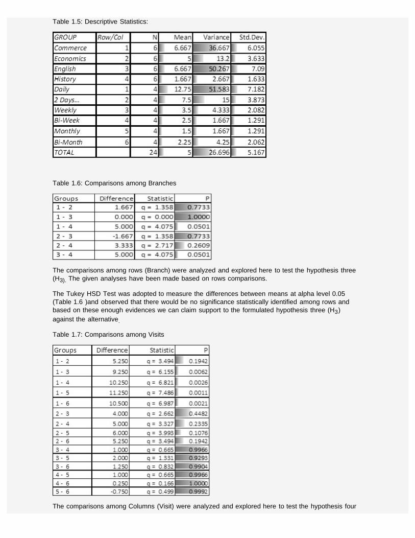
Table 1.5: Descriptive Statistics:

Table 1.6: Comparisons among Branches

The comparisons among rows (Branch) were analyzed and explored here to test the hypothesis three(H3). The given analyses have been made based on rows comparisons.

The Tukey HSD Test was adopted to measure the differences between means at alpha level 0.05(Table 1.6 )and observed that there would be no significance statistically identified among rows andbased on these enough evidences we can claim support to the formulated hypothesis three (H3)against the alternative.

Table 1.7: Comparisons among Visits

The comparisons among Columns (Visit) were analyzed and explored here to test the hypothesis four

(H4). The given analyses have been made based on Columns comparisons.

Table 1.7 depicts that there would be no significance statistically identified among columns at alphalevel 0.05, and based on these enough evidences, we can claim support to the formulated hypothesisfour (H4) against the alternative, except the groups 1-3,4,5,6 as they have secured enough statisticalevidences.

Comparisons among Visit within Each Branch

The comparisons among columns (visit) within each were analyzed and explored here to test thehypothesis five (H5).

Table 1.8: Row 1 Comparisons (Commerce)

Table 1.8 shows the test results that there would be no significance statistically identified amongcolumns within row (Commerce) and based on these enough evidences we can claim support to theformulated hypothesis five (H5) against the alternative, except the groups 1-4,5 as they have securedenough statistical evidences.

Table 1.8a: Row 2 Comparisons (Economics)

Table 1.8a shows the test results that there would be no significance statistically identified amongcolumns within row (Economics) and based on these enough evidences we can claim support to the

formulated hypothesis five (H5) against the alternative..

Table 1.8b: Row 3 Comparisons (English)

Table 1.8b shows the test results that there would be no significance statistically identified amongcolumns within row (English) and based on these enough evidences we can claim support to theformulated hypothesis five (H5) against the alternative, except the groups 1-3,4,5,6 as they havesecured enough statistical evidences.

Table 1.8c: Row 4 Comparisons (History)

Table 1.8c shows the test results that there would be no significance statistically identified amongcolumns within row (History) and based on these enough evidences we can claim support to theformulated hypothesis five (H5) against the alternative.

Comparisons among Branch within Each Visit

The comparisons among rows within each column (visit) were analyzed and explored here to test thehypothesis six (H6). The given analyses have been made based on column 1 comparisons.

Table 1.9: Column 1 Comparisons

The above Tukey HSD Test among pairs of means at alpha level 0.05 clearly indicates that therewould be no significance statistically identified among rows within each column(1) and based on theseenough evidences we can claim support to the formulated hypothesis six (H6) against the alternativeexcept the pairs 1-4 and 3-4 as they have secured enough evidences..

Table 1.9a: Column 2 Comparisons

Table 1.9a explores the Tukey HSD Test results at alpha level 0.05 that there would be no significancestatistically identified among rows within each column(2) and based on these enough evidences we canclaim support to the formulated hypothesis six (H6) against the alternative.

Table 1.9b: Column 3 Comparisons

Table 1.9c: Column 4 Comparisons

Table 1.9d: Column 5 Comparisons

Table 1.9e: Column 6 Comparisons

From the tables 1.9a-1.9e if could be inferred that at alpha level 0.05 there would be no significancestatistically identified among branches within each visit, and based on these enough evidences we canclaim support to the formulated hypothesis six (H6) that the groups of means among the brancheswithin Library visit are equal.

Table 2: Awareness of Internet

Table 2.1: Row Analysis:

Table 2.2: Col. Analysis:

Table 2.3: Total Analysis:

Respondents' awareness levels of Internet could be observed from the Table 2. In Commerce discipline57.50% of the users have adequate awareness followed by 'Insufficient' (25.00%) and 'I can manage'(17.50%). In Economics 56.67% of the respondents have adequate awareness followed by 'Insufficient'(36.67%), and rest of the level has secured 6.67%. The respondents from the branch 'English' havereceived the scores 52.50% (adequate), 30.00% (I can manage) and 17.50% (Insufficient) respectively.History branch has secured 40.0% for the option 'adequate', and rests of the options have received30.00% each. The columns and total analyses may explore more information about the dispersions ofthe observations. The observed points alone would never help the investigators to make the inferencesabout the population. Hence, a Two-Way ANOVA (Table 2.4) has been performed to trace thesignificance among the variables. From the ANOVA test results it is inferred that there would be nosignificance exist among the branch wise analysis (F=3.347(Fcrit =4.757)), which led us to claimsupport to the formulated hypothesis two (H2) against the alternative at the significance level of alpha0.05%. The analysis for the awareness levels did show up the significance as it has secured the Fvalue 6.038(Fcrit =5.143), which could be the reason for not claiming support to the hypothesis two(H2) in favor of the alternative. Distributions could be clearly observed from the plot distributions (SeeAnnexure-ii) which have been formulated for better capture.

Table 2.4: Two Way Analysis of Variance

Variable analyzed: Score/ Factor A (rows) variable: Branch/ Factor B (col.) variable: Awareness

SOURCE D.F. SS MS F Prob.> F Omega Squared

Among Branch 3 200 66.667 3.347 0.097 0.242

Among Awareness 2 240.5 120.25 6.038 0.037 0.346

Residual 6 119.5 19.917

NonAdditivity 1 60.923 60.923 5.2 0.072

Balance 5 58.577 11.715

Total 11 560 50.909

Omega squared for combined effects = 0.588

Table 2.5: Descriptive Statistics:

Table 2.6: Comparisons among awareness

The comparisons among columns (awareness) were analyzed and explored here to test the hypothesisfour (H4). The given analyses have been made based on rows comparisons.

Table 2.6 depicts that there would be no significance statistically identified among columns at alphalevel 0.05, and based on these enough evidences, we can claim support to the formulated hypothesisfour (H4) against the alternative, except the groups 1-2 as they have secured enough statisticalevidences to reject the same hypothesis..

Comparisons among Awareness within Each Branch

Table 2.7: Row 1 Comparisons

Table 2.7a: Row 2 Comparisons

Table 2.7b: Row 3 Comparisons

Table 2.7c: Row 4 Comparisons

Tables 2.7-2.7c depict that there would be no significance statistically identified among the awareness

within each row (Branch) at alpha level 0.05, and based on these enough evidences, we can claimsupport to the formulated hypothesis five (H5) that the groups of means among the awareness withineach branch are equal, against the alternative..

Comparisons among branch within each awareness levels

The comparisons among rows (Branch) within each column (awareness) were analyzed and exploredhere to test the hypothesis six (H6).

Table 2.8: Column 1 Comparisons (Adequate)

Table 2.8a: Column 2 Comparisons (I can manage)

Table 2.8b: Column 3 Comparisons (Insufficient)

Tables 2.8-2.8b depict that there would be no significance statistically identified among the brancheswithin each column (awareness) at alpha level 0.05, and based on these enough evidences, we canclaim support to the formulated hypothesis six (H6) that the groups of means among the brancheswithin each awareness are equal..

Pearson Coefficient of Correlation Test:

Table 3: Daily and Adequate

Daily and Adequate

Pearson Coefficient of Correlation 0.9145

t Stat 3.1958

df 2

P(T<=t) two tail 0.0856

t Critical two tail 4.3027

An evaluation was made of the linear relationship between the selected variables using Correlation.Test result indicates positive relationship between the variables. However, no statistically significantlinear relationship between Daily and Adequate as r(2)=0.9145, p = 0.086. Hence, we do not haveenough statistical evidences to claim support to the alternative against the formulated hypothesis seven(H7). Figure -3 Plots the combinations of two variables against one another for better capture.

Figure-3: Scatter Plot Distribution

Table 3.1: Daily and I can manage

Daily and I can manage

Pearson Coefficient of Correlation 0.8678

t Stat 2.4695

df 2

P(T<=t) two tail 0.1322

t Critical two tail 4.3027

An evaluation was made of the linear relationship between the selected variables using CorrelationAnalysis. Test result indicates positive relationship between the variables. However, no statisticallysignificant linear relationship between Daily and I Can Manage as r(2)=0.8678, p= 0.132. Hence, we donot have enough statistical evidences to claim support to the alternative against the formulatedhypothesis seven (H7). Figure -3.1 Plots the combinations of two variables against one another forbetter capture.

Figure-3.1: Scatter Plot Distribution

Table 3.2: Daily and Insufficient

Daily and Insufficient

Pearson Coefficient of Correlation 0.4746

t Stat 0.7625

df 2

P(T<=t) two tail 0.5254

t Critical two tail 4.3027

An evaluation was made of the linear relationship between the selected variables using CorrelationAnalysis. Test result indicates positive relationship between the variables. However, no statisticallysignificant linear relationship between Daily and Insufficient as r(2)=0.4746, p = 0.525. Hence, we donot have enough statistical evidences to claim support to the alternative against the formulatedhypothesis seven (H7). Figure -3.2 Plots the combinations of two variables against one another forbetter capture.

Figure-3.2: Scatter Plot Distribution

Table 4: Once in 2 Days and Adequate

Once in 2 Days and Adequate

Pearson Coefficient of Correlation 0.9525

t Stat 4.4217

df 2

P(T<=t) two tail 0.0476

t Critical two tail 4.3027

An evaluation was made of the linear relationship between the selected variables using CorrelationAnalysis. Test result indicates positive relationship between the variables and also statisticallysignificant linear relationship between Once in 2 Days and Adequate as r(2)=0.9525, p = 0.0476.Hence, we do not have enough statistical evidences to claim support to the formulated hypothesisseven (H7) as there would be a favor for the alternative. Figure-4 Plots the combinations of twovariables against one another for better capture.

Figure-4: Scatter Plot Distribution

Table 4.1: Once in 2 Days and I can manage

Once in 2 Days and I can manage

Pearson Coefficient of Correlation 0.3218

t Stat 0.4807

df 2

P(T<=t) two tail 0.6782

t Critical two tail 4.3027

An evaluation was made of the linear relationship between the selected variables using CorrelationAnalysis. Test result indicates positive relationship between the variables. However, no statisticallysignificant linear relationship between Daily and I can manage as r(2)=0.3218, p = 0.6782. Hence, wedo not have enough statistical evidences to claim support to the alternative against the formulatedhypothesis seven (H7). Figure -4.1 Plots the combinations of two variables against one another forbetter capture.

Figure-4.1: Scatter Plot Distribution

Table 4.2: Once in 2 Days and Insufficient

Once in 2 Days and Insufficient

Pearson Coefficient of Correlation 0.922

t Stat 3.367

df 2

P(T<=t) two tail 0.078

t Critical two tail 4.3027

An evaluation was made of the linear relationship between the selected variables using CorrelationAnalysis. Test result indicates positive relationship between the variables. However, no statisticallysignificant linear relationship between Daily and Insufficient as r(2)=0.922, p = 0.078. Hence, we do nothave enough statistical evidences to claim support to the alternative against the formulated hypothesisseven (H7). Figure -4.2 Plots the combinations of two variables against one another for better capture.

Figure-4.2: Scatter Plot Distribution

Table 5: Week and Adequate

Weekly and Adequate

Pearson Coefficient of Correlation 0.8532

t Stat 2.3136

df 2

P(T<=t) two tail 0.1468

t Critical two tail 4.3027

An evaluation was made of the linear relationship between the selected variables using CorrelationAnalysis. Test result indicates positive relationship between the variables. However, no statisticallysignificant linear relationship between Week and Adequate as r(2)=0.8532, p = 0.1468. Hence, we donot have enough statistical evidences to claim support to the alternative against the formulatedhypothesis seven (H7). Figure -5 Plots the combinations of two variables against one another for bettercapture.

Figure-5: Scatter Plot Distribution

Table 5.1: Week and I can manage

Weekly and I can manage

Pearson Coefficient of Correlation 0.8806

t Stat 2.6279

df 2

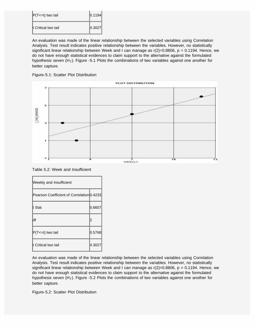
P(T<=t) two tail 0.1194

t Critical two tail 4.3027

An evaluation was made of the linear relationship between the selected variables using CorrelationAnalysis. Test result indicates positive relationship between the variables. However, no statisticallysignificant linear relationship between Week and I can manage as r(2)=0.8806, p = 0.1194. Hence, wedo not have enough statistical evidences to claim support to the alternative against the formulatedhypothesis seven (H7). Figure -5.1 Plots the combinations of two variables against one another forbetter capture.

Figure-5.1: Scatter Plot Distribution

Table 5.2: Week and Insufficient

Weekly and Insufficient

Pearson Coefficient of Correlation 0.4233

t Stat 0.6607

df 2

P(T<=t) two tail 0.5768

t Critical two tail 4.3027

An evaluation was made of the linear relationship between the selected variables using CorrelationAnalysis. Test result indicates positive relationship between the variables. However, no statisticallysignificant linear relationship between Week and I can manage as r(2)=0.8806, p = 0.1194. Hence, wedo not have enough statistical evidences to claim support to the alternative against the formulatedhypothesis seven (H7). Figure -5.2 Plots the combinations of two variables against one another forbetter capture.

Figure-5.2: Scatter Plot Distribution

Table 6: Bi-Week and Adequate

Bi-Week and Adequate

Pearson Coefficient of Correlation -0.1058

t Stat -0.1505

df 2

P(T<=t) two tail 0.8942

t Critical two tail 4.3027

An evaluation was made of the linear relationship between the selected variables using Correlationanalysis. Test result indicates the negative and weak relationship between the variables Bi-Week andAdequate as r(2)=-0.1058, p = 0.8942. With the help of enough statistical evidences it is inferred thatthere would not be a possible significance statistically identified to claim support to the alternativeagainst the formulated hypothesis seven (H7). Figure -6 Plots the combinations of two variables againstone another for better capture.

Figure-6: Scatter Plot Distribution

Table 6.1: Bi- Week and I can manage

Bi-Week and I can manage

Pearson Coefficient of Correlation 0.7384

t Stat 1.5483

df 2

P(T<=t) two tail 0.2616

t Critical two tail 4.3027

An evaluation was made of the linear relationship between the selected variables using CorrelationAnalysis. Test result indicates positive relationship between the variables. However, no statisticallysignificant linear relationship between Bi-Week and I can manage as r(2)=0.7384, p = 0.2616. Hence,we do not have enough statistical evidences to claim support to the alternative against the formulatedhypothesis seven (H7). Figure -6.1 Plots the combinations of two variables against one another forbetter capture.

Figure-6.1: Scatter Plot Distribution

Table 6.2: Bi-Week and Insufficient

Bi-Week and Insufficient

Pearson Coefficient of Correlation -0.6825

t Stat -1.3206

df 2

P(T<=t) two tail 0.3174

t Critical two tail 4.3027

An evaluation was made of the linear relationship between the selected variables using Correlationanalysis. Test result indicates the negative and weak relationship between the variables Bi-Week andInsufficient as r(2)=-0.6825, p = 0.3174. With the help of enough statistical evidences it is inferred thatthere would not be a possible significance statistically identified to claim support to the alternativeagainst the formulated hypothesis seven (H7). Figure -6.2 Plots the combinations of two variablesagainst one another for better capture.

Figure-6.2: Scatter Plot Distribution

Table 7: Monthly and Adequate

Monthly and Adequate

Pearson Coefficient of Correlation 0.6199

t Stat 1.1171

df 2

P(T<=t) two tail 0.3802

t Critical two tail 4.3027

An evaluation was made of the linear relationship between the selected variables using CorrelationAnalysis. Test result indicates positive relationship between the variables. However, no statisticallysignificant linear relationship between Monthly and Adequate as r(2)=0.6199, p = 0.3802. Hence, we donot have enough statistical evidences to claim support to the alternative against the formulatedhypothesis seven (H7). Figure -7 Plots the combinations of two variables against one another for bettercapture.

Figure-7: Scatter Plot Distribution

Table 7.1: Monthly and I can manage

Monthly and I can manage

Pearson Coefficient of Correlation -0.2272

t Stat -0.3299

df 2

P(T<=t) two tail 0.7728

t Critical two tail 4.3027

An evaluation was made of the linear relationship between the selected variables using Correlationanalysis. Test result indicates the negative and weak relationship between the variables Monthly and Ican manage as r(2)=-0.2272, p = 0.7728. With the help of enough statistical evidences it is inferredthat there would not be a possible significance statistically identified to claim support to the alternativeagainst the formulated hypothesis seven (H7). Figure -7.1 Plots the combinations of two variablesagainst one another for better capture.

Figure-7.1: Scatter Plot Distribution

Table 7.2: Monthly and Insufficient

Monthly and insufficient

Pearson Coefficient of Correlation 0.969

t Stat 5.629

df 2

P(T<=t) two tail 0.03

t Critical two tail 4.3027

An evaluation was made of the linear relationship between the selected variables using CorrelationAnalysis. Test result indicates positive relationship between the variables. Also, there would be astatistically significant linear relationship between Monthly and Insufficient as r(2)=0.969, p = 0.03.Hence, we do not have enough statistical evidences to claim support to the formulated hypothesisseven (H7) against the alternative. Figure -7.2 Plots the combinations of two variables against oneanother for better capture.

Figure-7.2: Scatter Plot Distribution

Table 8: Bi-Month and Adequate

Bi-Month and Adequate

Pearson Coefficient of Correlation 0.658

t Stat 1.2358

df 2

P(T<=t) two tail 0.342

t Critical two tail 4.3027

An evaluation was made of the linear relationship between the selected variables using CorrelationAnalysis. Test result indicates positive relationship between the variables. However, no statisticallysignificant linear relationship between Bi-Month and Adequate as r(2)=0.658, p = 0.342. Hence, we donot have enough statistical evidences to claim support to the alternative against the formulatedhypothesis seven (H7). Figure -8 Plots the combinations of two variables against one another for bettercapture.

Figure-8: Scatter Plot Distribution

Table 8.1: Bi-Month and I can manage

Bi-Month and I can manage

Pearson Coefficient of Correlation -0.2134

t Stat -0.3089

df 2

P(T<=t) two tail 0.7866

t Critical two tail 4.3027

An evaluation was made of the linear relationship between the selected variables using Correlationanalysis. Test result indicates the negative and weak relationship between the variables Bi-Month and Ican manage as r(2)=-0.2134, p = 0.7866. With the help of enough statistical evidences it is inferredthat there would not be a possible significance statistically identified to claim support to the alternativeagainst the formulated hypothesis seven (H7). Figure -8.1 Plots the combinations of two variablesagainst one another for better capture.

Figure-8.1: Scatter Plot Distribution

Table 8.2: Bi-Month and Insufficient

Bi-Month and Insufficient

Pearson Coefficient of Correlation 0.956

t Stat 4.6098

df 2

P(T<=t) two tail 0.044

t Critical two tail 4.3027

An evaluation was made of the linear relationship between the selected variables using Correlationanalysis. Test result indicates the strong relationship between the variables Bi-Month and Insufficientas r(2)=-0.956, p = 0.044. With the help of enough statistical evidences it is inferred that there wouldnot be a possible significance statistically identified to claim support to the alternative against theformulated hypothesis seven (H7). Figure -8.2 Plots the combinations of two variables against oneanother for better capture.

Figure-8.2: Scatter Plot Distribution

Determinations:

The present study encompasses the sample size up to 120 comprising the disciplines of Commerce,Economics, English and History. The study reveals that the respondents' daily visit to the library toutilize the IT infrastructures has secured the first slot as the mean value is traced as 12.75 withStd.Dev. 7.182. Respondents' 2 days once visit received the mean 7.5, and Std.Dev. 3.873. The Weekwise visit to the library has secured the mean and Std.Dev. 3.5, 2.082 followed by Bi-Week (2.5,1.291), Bi-Month (2.25, 2.062) and rest of the attribute month have the least values (1.5, 1.291). Itcould be inferred from the analysis that the majority of respondents would like to visit the library daily inorder to access the electronic features that are offered in the library. Two-Way Anova was applied tofulfill the research question; do the modern users' Library visits differ? , and the results (F=3.69, 8.38)made us to conclude that there would be a possible significance exist between the users visit to thelibrary. The calculated w2 shows approximately 11 per cent of variance for the variable Branch while

53 per cent of variance exists in Library visits. The w2 for combined effects is traced as 0.652. Further,we were interested to trace the specific groups in which the significance exist, and hence the Post-HocTest namely Tukey HSD was adopted to analyze the pairs. The visit wise comparison test resultsrevealed that the groups 1-3, 4, 5, 6 (Table 1.7) did show the significance rather than other pairs. TheComparisons among visit within each branch test results revealed that the groups 1- 4, 5 (Table 1.8a);the groups 1-3, 4, 5, 6 (Table 1.8c) have come up with the significance while other pairs didn't showthe significance. The Comparisons among branch within each visit test results showed that the groups1- 4 & 3-4 (Table 1.9) are having significance when compared to the remaining pairs.

The analysis for the attributes 'Internet awareness' reveal that majority of respondents have gotadequate awareness (mean=16.25, Std.Dev.=8.539) of Internet whereas the rest of the users felt thatthey have insufficient knowledge of the Internet (mean=7.75, Std.Dev.=3.594) followed by the level 'Ican manage', which has received the mean 6 with the Std.Dev.4.546. Two-Way Anova was againapplied to test the research question, do the users' Internet awareness levels differ? , and the resultsfor rows (F=3.347, 6.038) made us to conclude that there would not be a possible significance existbetween the users' awareness levels. In contrary the results for columns (F=6.038) would not led us toconclude the same. To trace the significance for the pairs, we once again used the Post-Hoc Test(Tukey HSD). The awareness wise comparison test results indicates possible significance for thegroups 1-2 (Table 2.6) rather than other pairs. The statistical tool namely Pearson's correlationcoefficient has been adopted to test the research question, do the users' Library visits influence them toupgrade their awareness of Internet? , and the outcomes were explored towards the Tables 3-8.2.Correlation Test result indicates positive as well as statistically significant linear relationship betweenthe variables (Table 4) Once in 2 Days and Adequate as r(2)=0.9525, p = 0.0476 ; (Table 7.2) Monthlyand Insufficient as r(2)=0.969, p = 0.03, and (Table 8.2) Bi-Month and Insufficient as r(2)=-0.956, p =0.044. Though some of the strong/weak and positive/negative relationships were identified between thevariables thorough out the study the possible significance was not captured in between the levels ofthe variables except a few levels. It would be interesting to observe the above results that the frequentvisits to the library enable one to be aware of the Internet, when compared to the Bi-Month and Monthwise visits. Hence, it could be concluded that there would be linear relationship exist between theusers' library visits and their awareness of Internet. Of course, the electronic environment setups insidethe library upgrade the modern users' Internet awareness.

Acknowledgements

I sincerely express my thanks to Professor Emeritus William G. Miller, Lowa State University.

References

1. Ricco RAKOTOMALALA.(2005). Tanagra: Un logiciel gratuit pour l'enseignement et la recherche. inActes de EGC'2005, RNTI-E-3.vol-2. Pp.697-702.

2. Saravanan, T. (2010). Google Use and Users: A Survey. Information Studies. Vol.16. N.1. Pp.49-64.

3. Saravanan T and Gopalakrishnan, S.(2011). Higher education user's awareness of Google:Searching for Structure. Library Progress (International). Vol.31. N.1. Pp.91-97.

4. TexaSoft. (2007) WINKS SDA, 6th ed., Cedar Hill, Texas.

5. William G. Miller.(2009). Statistics and Measurement Using Openstat.

Appendix 1

Figure 1: Branch wise 3D Distribution

Figure 2: Library Visit-3D Distribution

Figure 3: Branch Vs Visit 3D Distribution

Appendix 2

Figure 4: Branch Mean Distribution

Figure 5: Awareness Mean Distribution

Figure 6: Branch Vs Awareness Mean Distribution