Does Student Sorting Invalidate Value-Added Models of Teacher Effectiveness?

An Extended Analysis of the Rothstein Critique

Cory Koedel

University of Missouri

Julian R. Betts*

University of California, San Diego

National Bureau of Economic Research

July 2009

Value-added modeling continues to gain traction as a tool for measuring

teacher performance. However, recent research (Rothstein, 2009a,

2009b) questions the validity of the value-added approach by showing

that it does not mitigate student-teacher sorting bias (its presumed

primary benefit). Our study explores this critique in more detail.

Although we find that estimated teacher effects from some value-added

models are severely biased, we also show that a sufficiently complex

value-added model that evaluates teachers over multiple years reduces

the sorting-bias problem to statistical insignificance. One implication of

our findings is that data from the first year or two of classroom teaching

for novice teachers may be insufficient to make reliable judgments about

quality. Overall, our results suggest that in some cases value-added

modeling will continue to provide useful information about the

effectiveness of educational inputs.

* The authors thank Andrew Zau and many administrators at San Diego Unified School District

(SDUSD), in particular Karen Bachofer and Peter Bell, for helpful conversations and assistance

with data issues. We also thank Zack Miller, Shawn Ni, Mike Podgursky, seminar participants at

Northwestern University and Simon Fraser University, and two anonymous referees for useful

comments and suggestions, and the National Center for Performance Incentives for research

support. SDUSD does not have an achievement-based merit pay program, nor does it use value-

added student achievement data to evaluate teacher effectiveness. The underlying project that

provided the data for this study has been funded by a number of organizations including The

William and Flora Hewlett Foundation, the Public Policy Institute of California, The Bill and

Melinda Gates Foundation, the Atlantic Philanthropies and the Girard Foundation. None of

these entities has funded the specific research described here, but we warmly acknowledge their

contributions to the work needed to create the database underlying the research.

1

Economic theory states that in an efficient economy workers should be paid their value

marginal product. Implementing this rule in the service sector is not simple, as it is often not

obvious how to measure the output of a white collar worker. Teachers provide an example of

this problem: public school teachers‟ salaries are determined largely by academic degrees and

credentials, and years of experience, none of which appears to be strongly related to teaching

effectiveness.

Perhaps in recognition that teacher pay is not well aligned with teaching quality,

President Obama has recently called for greater use of teacher merit pay as a tool to boost

student achievement in America‟s public schools. And yet, in the United States, teacher merit

pay is hardly a new idea. It has been used for at least a century, but most programs are short-

lived, or survive either by giving almost all teachers bonuses or by giving trivial bonuses to a

small number of teachers. Teachers have traditionally complained that principals cannot explain

why they gave a bonus to one teacher but not another (Murnane et al., 1991, pp. 117-119).

Opponents of teacher merit pay would raise the question of whether we can reliably measure

teachers‟ value marginal products such that informed merit-pay decisions can be made.

The advent of widescale student testing, partly in response to the requirements of the

federal No Child Left Behind law, raises the possibility that it is now feasible to measure the

effectiveness of individual teachers. Indeed, recently developed panel datasets link students and

teachers at the classroom level, allowing researchers to estimate measures of „outcome-based‟

teacher effectiveness.1 Because test scores are generally available for each student in each year,

they lend themselves comfortably to a “value-added” approach where the effectiveness of

teacher inputs can be measured by student test-score growth. The conjuncture of President

1 For recent examples see Aaronson, Barrow and Sander (2007), Hanushek, Kain, O‟Brien and Rivkin (2005), Harris

and Sass (2006), Koedel and Betts (2007), Nye, Konstantopoulos and Hedges (2004), and Rockoff (2004).

2

Obama‟s recent calls for teacher merit pay and the development of panel datasets that provide

information on student achievement growth raise the stakes considerably: can we use student

testing to reliably infer teaching quality?

In most schools, students are not randomly assigned to teachers. A presumption in value-

added modeling is that by focusing on achievement growth rather than achievement levels, the

problem of student-teacher sorting bias is resolved because each student‟s initial test-score level

is used as a control in the model. The value-added approach is intuitively appealing, and

increasing demand for performance-based measures by which teachers can be held accountable -

at the federal, state and district levels – has only fueled the value-added fire.2 However, despite

the popularity of the value-added approach among both researchers and policymakers, not

everyone agrees that it is reliable. Couldn‟t it be the case that a given teacher either

systematically or occasionally receives students whose gains in test scores are unusually low, for

reasons outside the control of the teacher? Ability grouping would be one source of persistent

differences in the types of students across classrooms. Random variations, accompanied by

mean reversion, would be a source of fleeting differences that a value-added model might

wrongly attribute to a given teacher.

Recent research by Rothstein (2009a) shows that future teacher assignments have non-

negligible predictive power over current student performance in value-added models, despite the

fact that future teachers cannot possibly have causal effects on current student performance.

This result suggests that student-teacher sorting bias is not mitigated by the value-added

approach. Rothstein‟s critique of the value-added methodology comes as numerous studies have

2 No Child Left Behind legislation is one example of this demand at the federal level (e.g., adequate yearly

progress), and states such as Florida, Minnesota and Texas have all introduced performance incentives for teachers

that depend to some extent on value-added. For a further discussion of the performance-pay landscape, particularly

as it relates to teachers, see Podgursky and Springer (2007).

3

used and continue to use the technique. It raises serious doubts about the value-added

methodology just as other work, such as Kane and Staiger (2008), Jacob and Lefgren (2007) and

Harris and Sass (2007), appears to confirm that value-added is a meaningful measure of teacher

performance.

We further explore the reliability of value-added modeling by extending Rothstein‟s

analysis in two important ways. First, Rothstein estimates teacher effects using only a single

year of data for each teacher. We consider the importance of using multiple years of data to

identify teacher effects. If the sorting bias uncovered by Rothstein is transitory to some extent,

using multiple cohorts of students to evaluate teachers will help mitigate the bias.3 For example,

a principal may alternate across years in assigning the most troublesome students to the teachers

at her school, or teachers may connect with their classrooms more in some years than in others.4

These types of single-year idiosyncrasies will be captured by single-year teacher effects, but will

be smoothed out if estimates are based on multiple years of data. Second, we evaluate the

Rothstein critique using a different dataset. Given that the degree of student-teacher sorting may

differ across different educational environments, his results may or may not be replicated in

other settings.

Our extension of Rothstein‟s analysis corroborates his primary finding – value-added

models of student achievement that focus on single-year teacher effects will generally produce

biased estimates of value-added. However, when we estimate a detailed value-added model and

restrict our analysis to teachers who teach multiple classrooms of students, we find no evidence

3 Rothstein notes this in his appendix, although he does not explore the practical implications in any of his models.

4 Additionally, some of what we observe to be sorting bias may be attributable to the random assignment of students

to teachers across small samples (classrooms). In an omitted analysis, we perform a Monte Carlo exercise to test for

this possibility. Although any given teacher may benefit (be harmed) in any given year from a random draw of high-

performing (low-performing) students, we find no evidence to suggest that this would influence estimates of the

distribution of teacher effects.

4

of sorting bias in the estimated teacher effects. Although this result depends on the degree of

student-teacher sorting in our data, it suggests that at least in our setting, sorting bias can be

almost completely mitigated using the value-added approach and looking across multiple years

of classrooms for teachers.

Our results in this regard are encouraging, but less detailed value-added models that

include teacher-effect estimates based on single classroom observations fare poorly in our

analysis. That some value-added models will be reliable but not others, and that value-added

modeling may only be reliable in some settings, are important limitations. They suggest that in

contexts such as statewide teacher-accountability systems, large-scale value-added modeling

may not be a viable solution. Because the success of the value-added approach will depend

largely on data availability and the underlying degree of student-teacher sorting in the data

(much of which may be unobserved), post-estimation falsification tests along the lines of those

proposed by Rothstein (2009a) will be useful in evaluating the reliability of value-added

modeling in different contexts.

Although we do not uncover a well-defined set of conditions under which value-added

modeling will universally return causal teacher effects across different schooling environments

(outside of random student-teacher assignments such conditions are unlikely to exist), we do

identify conditions under which value-added estimation will perform better. The most important

insight is that teacher evaluations that span multiple years will produce more reliable measures of

teacher effectiveness than those based on single-year classroom observations. Often implicitly,

the value-added discussion in research and policy revolves around single-year estimates of

teacher effects. Our analysis strongly discourages such an approach.

5

The remainder of the paper is organized as follows. Section I briefly describes the

Rothstein critique. Section II details our dataset from the San Diego Unified School District

(SDUSD). Section III replicates a portion of Rothstein‟s analysis using the San Diego data.

Section IV details our extended analysis of value-added modeling and presents our results.

Section V uses these results to estimate the variance of teacher effectiveness in San Diego.

Section VI concludes.

I. The Rothstein Critique

Rothstein raises concerns about assigning a causal interpretation to value-added estimates

of teacher effects. His primary argument is that teacher effects estimated from value-added

models are biased by non-random student-teacher assignments, and that this bias is not removed

by the general value-added approach, nor by standard panel-data techniques. Consider a simple

value-added model of the general form:

(1) 1 ( )it it it it i itY Y X T

In equation (1), Yit is a test-score for student i in year t, Xit is a vector of time-varying

student and school characteristics (for the school attended by student i in year t), and Tit is a

vector of indicator variables indicating which teacher(s) taught student i in year t. This model

could be re-formulated as a “gainscore” model by forcing the coefficient on the lagged test score

to unity and moving it to the left-hand side of the equation. The error term is written as the sum

of two components, one that is time-invariant ( i ) and another that varies over time ( it ).

Rothstein discusses sorting bias as coming from two different sources in this basic model.

First, students could be assigned to teachers based on “static” student characteristics. This type

of sorting corresponds to the typical tracking story – some students are of higher ability than

others, and these students are systematically assigned to the best teachers. Static tracking may

6

operationalize in a variety of ways including administrator preferences, parental preferences, or

teacher preferences (assuming that primary-school aged children, upon whom we focus here, are

not yet able to form their own preferences). Given panel data, the typical solution to the static-

tracking problem is the inclusion of student fixed effects, which control for the time-invariant

components to the error terms in equation (1). If student-teacher sorting is based only on static

student characteristics, this approach will be sufficient.

However, the student-fixed-effects solution to the static tracking problem necessarily

imposes a strict exogeneity assumption. That is, to uncover causal teacher effects from a model

that controls for time-invariant student characteristics, it must be the case that teacher

assignments in all periods are uncorrelated with the time-varying error components in all periods.

To see this, note that we could estimate equation (1) by first differencing to remove the time-

invariant component to the error term:5

(2) 1 1 2 1 1 1( ) ( ) ( ) ( )it it it it it it it it it itY Y Y Y X X T T

The first-differencing induces a mechanical correlation between the lagged test-score gain and

the first-differenced error term in equation (2). This correlation can be resolved by

instrumenting for the lagged test-score gain with the second-lagged gain, or second-lagged level

(following Anderson and Hsiao, 1981). In addition, year-t teacher assignments may also be

correlated with the first-differenced error term. Specifically, if students are sorted dynamically

based on time-varying deviations (or shocks) to their test-score-growth trajectories, then lagged

shocks to test-score growth, captured by 1it , will be correlated with year-t teacher assignments,

5 In the case of first differencing, it is more accurate to describe the assumption as “local” strict exogeneity in the

sense that the error terms across time must be uncorrelated with teacher assignments only in contiguous years.

7

and the teacher effects from equation (2) cannot be given a causal interpretation.6 Rothstein‟s

critique can be summarized as follows: If students are assigned to teachers based entirely on

time-invariant factors, unbiased teacher effects can in principle be obtained from a well-

constructed value-added model. However, if sorting is based on dynamic factors that are

unobserved by the econometrician, value-added estimates of teacher effects cannot be given a

causal interpretation.

Rothstein proposes a falsification test to determine whether value-added models produce

biased estimates of teacher effectiveness. He suggests simply adding future teacher assignments

to the model, and testing whether these teacher assignments have non-zero “effects”. Future

teachers do not causally influence current test scores, which means that any observed “effects”

must be the result of a correlation between teacher assignments and the error terms.

Alternatively, if the coefficients on the future-teacher indicator variables are jointly insignificant,

sorting bias is unlikely to be a major concern for any teacher effects in the model (as this finding

would suggest that the controls in the model are capturing the sorting bias that would otherwise

confound the teacher effects). In Rothstein‟s analysis (2009a), his most provocative finding is

that future teacher assignments have significant predictive power over current student

performance. This result suggests that value-added estimates of teacher effects are contaminated

by substantial sorting bias.

II. Data

We use administrative data from four cohorts of fourth-grade students in San Diego (at

the San Diego Unified School District) who started the fourth grade in the school years between

1998-1999 and 2001-2002. The standardized test that we use to measure student achievement,

6 Serial correlation in the epsilons would imply that if year-t teacher assignments are correlated with 1it then they

will also be correlated with it , invalidating any value-added model even in the absence of static tracking.

8

and therefore teacher value-added, is the Stanford 9 mathematics test. The Stanford 9 is

designed to be vertically scaled such that a one-point gain in student performance at any point in

the schooling process is meant to correspond to the same amount of learning.7

Students who have fourth-grade test scores and lagged test scores are included in our

baseline dataset. We estimate a value-added model that assumes a common intercept across

students, and a second model that incorporates student fixed effects. In this latter model we

additionally require students to have second-lagged test scores. For each of our primary models,

we estimate value-added for teachers who teach at least 20 students across the data panel and

restrict our student sample to the set of fourth-grade students taught by these teachers.8 In the

baseline dataset, we evaluate test-score records for 30,354 students taught by 595 fourth-grade

teachers. Our sample size falls to 15,592 students taught by 389 teachers in the student-fixed-

effects dataset. The large reduction in sample size is the result of (1) the requirement of three

contiguous test-score records per student instead of just two, which in addition to removing more

transient students also removes one year-cohort of students because we do not have test-score

data prior to 1997-1998 (that is, students in the fourth grade in 1998-1999 can have lagged scores

but not second-lagged scores) and (2) requiring the remaining students be assigned to one of the

389 fourth-grade teachers who teach at least 20 students with three test-score records or more.9

We include students who repeat the fourth grade because it is unlikely that grade repeaters would

be excluded from teacher evaluations in practice. In our original sample of 30,354 students with

current and lagged test-score records, only 199 are grade repeaters.

7 For detailed information about the quantitative properties of the Stanford 9 exam, see Koedel and Betts

(forthcoming). 8 This restriction is imposed because of concerns about sampling variation (see Kane and Staiger, 2002). Our results

are not sensitive to reasonable adjustments to the 20-student threshold. 9 Only students who repeated the 4

th grade in the latter two years of our panel could possibly have had more than

three test-score records. There are 32 students with four test-score records in our dataset.

9

III. Replication of Rothstein’s Analysis

Based on details provided by Rothstein in his paper (2009a) and corresponding data appendix,

we first replicate a portion of his analysis using data from the 1999-2000 fourth-grade cohort in

San Diego. This replication is meant to establish the extent to which Rothstein‟s underlying

findings are relevant in San Diego.10

We estimate the following basic value-added model:

(3) 4 3 3 4 4 5 5

i i i i i iY S T T T

Equation (3) is a gainscore model and corresponds to Rothstein‟s “VAM1” model with

indicators for past, current and future teacher assignments. 4

iY represents a student‟s test-score

gain going from the third to fourth grade, Si is a vector of school indicator variables, and x

iT is a

vector of teacher indicator variables for student i in grade x. Correspondingly, x is a vector of

teacher effects corresponding to the set of teachers who teach grade x. Rothstein‟s basic

argument is that if future teacher effects, for fifth-grade teachers in this case, are shown to be

non-zero then none of the teacher effects in the model can be given a causal interpretation.11

We replicate the data conditions in Rothstein (2009a) as closely as possible when

estimating this model. There are two conditions that seemed particularly important. First, in

specifications that include teacher identifiers across multiple grades, Rothstein excludes students

who changed schools across those grades in the data. Second, he also focuses on only a single

cohort of students passing through the North Carolina public schools. Similarly to Rothstein, the

dataset used to estimate equation (3) does not include any school switchers, and is estimated

using just a single cohort of fourth-grade students in San Diego.

10

The replication data sample is roughly a subsample of the student-fixed-effects dataset, but we use different

teachers because Rothstein does not require teachers to teach 20 students for inclusion into the model. 11

Rothstein‟s analyses (2009b, 2009a) are quite thorough and we refer the interested reader to his paper for more

details.

10

In our replication we focus on the effects of fourth and fifth-grade teachers in equation

(3). In accordance with the literature that measures the importance of teacher value-added, we

report the adjusted and unadjusted variance of the teacher effects. We follow Rothstein‟s

approach to reporting the teacher-effect variances, borrowed from Aaronson, Barrow and Sander

(2007), where the unadjusted variance is just the raw variance of the teacher effects and the

adjusted variance is equal to the raw variance minus the average of the square of the robust

standard errors. We follow the steps outlined in Rothstein‟s appendix to estimate the within-

school variance of teacher effects without teachers switching schools. Our results are detailed in

Table 1.

The first two columns of Table 1 report the results of separate Wald tests of the

hypotheses that all grade 4 teachers have identical effects and that all grade 5 teachers have

identical effects. Confirming Rothstein‟s findings, the null hypothesis that grade 5 teachers have

an equal effect on students‟ gains in grade 4 is rejected with a p-value below 0.01.

The next two columns show the raw standard deviations of teacher effects and the

standard deviations after adjusting for sampling variance. (These are scaled by dividing by the

standard deviation of student test scores.) The adjusted standard deviations are 0.24 and 0.15 for

grade 4 and grade 5 teachers respectively. Rothstein‟s estimates that are most analogous to those

in our Table 1, both in terms of the model and data, are reported in his Table 5 (column 2) for the

“unrestricted model”. There, he shows adjusted standard deviations of the distributions of grade

4 and grade 5 teacher effects of 0.193 and 0.099 standard deviations of the test, respectively.

These results are also replicated virtually identically in his Table 2 (column 7) where he uses a

larger student sample and excludes lagged-year teacher identifiers from the model. Our

estimates, which show a larger overall variance of teacher effects, are consistent with past work

11

using San Diego data (Koedel and Betts, 2007). The relevant result to compare with Rothstein

(2009a) is our estimate of the ratio of the standard deviations of the distributions of future and

current teacher effects. Rothstein finds that the standard deviation of the distribution of future

teacher “effects” is approximately 51 percent of the size of that of current teacher effects (i.e.,

0.099/0.193), whereas in our analysis this number is slightly higher at roughly 63 percent

(0.15/0.24). Our results here confirm Rothstein‟s findings that future teachers explain a sizeable

portion of current grade achievement gains, and establish that his primary result is not unique to

North Carolina.

The results in Table 1, and the corresponding results detailed by Rothstein, suggest that

student-teacher sorting bias is a significant complication to value-added modeling. Information

about the degree of student-teacher sorting in our data will be useful for generalizing our results

to other settings. We document observable student-teacher sorting in our data by comparing the

average realized within-teacher standard deviation of students‟ lagged test scores to analogous

measures based on simulated student-teacher matches that are either randomly generated or

perfectly sorted. This approach follows Aaronson, Barrow and Sander (2007). Although sorting

may occur along many dimensions, the extent of sorting based on lagged test scores is likely to

provide some indication of sorting more generally. Table 2 details our results, which are

presented as ratios of the standard deviation of interest to the within-grade standard deviation of

the test (calculated based on our student sample). Note that while there does appear to be some

student sorting based on lagged test-score performance in our dataset, this sorting is relatively

mild.

12

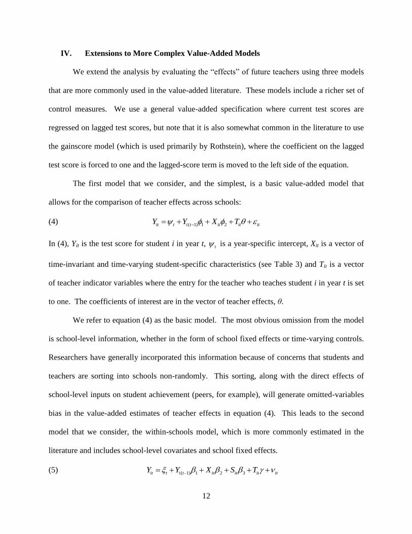
IV. Extensions to More Complex Value-Added Models

We extend the analysis by evaluating the “effects” of future teachers using three models

that are more commonly used in the value-added literature. These models include a richer set of

control measures. We use a general value-added specification where current test scores are

regressed on lagged test scores, but note that it is also somewhat common in the literature to use

the gainscore model (which is used primarily by Rothstein), where the coefficient on the lagged

test score is forced to one and the lagged-score term is moved to the left side of the equation.

The first model that we consider, and the simplest, is a basic value-added model that

allows for the comparison of teacher effects across schools:

(4) ( 1) 1 2it t i t it it itY Y X T

In (4), Yit is the test score for student i in year t, t is a year-specific intercept, Xit is a vector of

time-invariant and time-varying student-specific characteristics (see Table 3) and Tit is a vector

of teacher indicator variables where the entry for the teacher who teaches student i in year t is set

to one. The coefficients of interest are in the vector of teacher effects, θ.

We refer to equation (4) as the basic model. The most obvious omission from the model

is school-level information, whether in the form of school fixed effects or time-varying controls.

Researchers have generally incorporated this information because of concerns that students and

teachers are sorting into schools non-randomly. This sorting, along with the direct effects of

school-level inputs on student achievement (peers, for example), will generate omitted-variables

bias in the value-added estimates of teacher effects in equation (4). This leads to the second

model that we consider, the within-schools model, which is more commonly estimated in the

literature and includes school-level covariates and school fixed effects.

(5) ( 1) 1 2 3it t i t it it it itY Y X S T

13

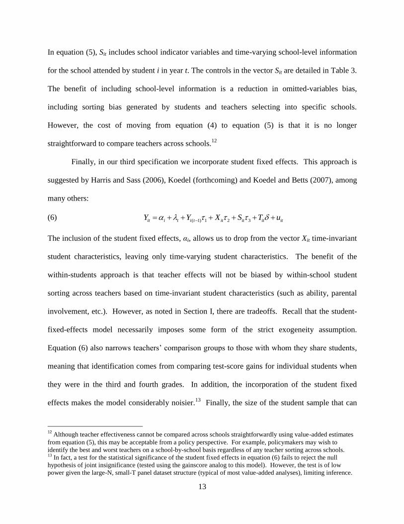
In equation (5), Sit includes school indicator variables and time-varying school-level information

for the school attended by student i in year t. The controls in the vector Sit are detailed in Table 3.

The benefit of including school-level information is a reduction in omitted-variables bias,

including sorting bias generated by students and teachers selecting into specific schools.

However, the cost of moving from equation (4) to equation (5) is that it is no longer

straightforward to compare teachers across schools.12

Finally, in our third specification we incorporate student fixed effects. This approach is

suggested by Harris and Sass (2006), Koedel (forthcoming) and Koedel and Betts (2007), among

many others:

(6) ( 1) 1 2 3it i t i t it it it itY Y X S T u

The inclusion of the student fixed effects, αi, allows us to drop from the vector Xit time-invariant

student characteristics, leaving only time-varying student characteristics. The benefit of the

within-students approach is that teacher effects will not be biased by within-school student

sorting across teachers based on time-invariant student characteristics (such as ability, parental

involvement, etc.). However, as noted in Section I, there are tradeoffs. Recall that the student-

fixed-effects model necessarily imposes some form of the strict exogeneity assumption.

Equation (6) also narrows teachers‟ comparison groups to those with whom they share students,

meaning that identification comes from comparing test-score gains for individual students when

they were in the third and fourth grades. In addition, the incorporation of the student fixed

effects makes the model considerably noisier.13

Finally, the size of the student sample that can

12

Although teacher effectiveness cannot be compared across schools straightforwardly using value-added estimates

from equation (5), this may be acceptable from a policy perspective. For example, policymakers may wish to

identify the best and worst teachers on a school-by-school basis regardless of any teacher sorting across schools. 13

In fact, a test for the statistical significance of the student fixed effects in equation (6) fails to reject the null

hypothesis of joint insignificance (tested using the gainscore analog to this model). However, the test is of low

power given the large-N, small-T panel dataset structure (typical of most value-added analyses), limiting inference.

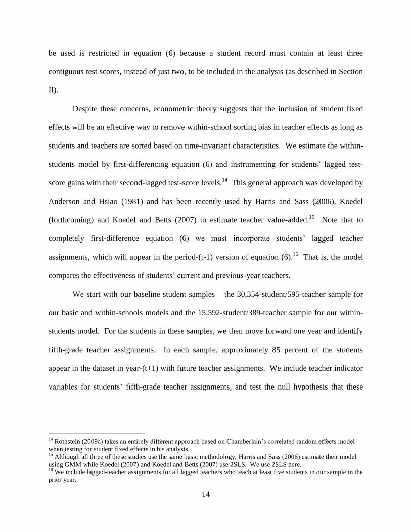
14

be used is restricted in equation (6) because a student record must contain at least three

contiguous test scores, instead of just two, to be included in the analysis (as described in Section

II).

Despite these concerns, econometric theory suggests that the inclusion of student fixed

effects will be an effective way to remove within-school sorting bias in teacher effects as long as

students and teachers are sorted based on time-invariant characteristics. We estimate the within-

students model by first-differencing equation (6) and instrumenting for students‟ lagged test-

score gains with their second-lagged test-score levels.14

This general approach was developed by

Anderson and Hsiao (1981) and has been recently used by Harris and Sass (2006), Koedel

(forthcoming) and Koedel and Betts (2007) to estimate teacher value-added.15

Note that to

completely first-difference equation (6) we must incorporate students‟ lagged teacher

assignments, which will appear in the period-(t-1) version of equation (6).16

That is, the model

compares the effectiveness of students‟ current and previous-year teachers.

We start with our baseline student samples – the 30,354-student/595-teacher sample for

our basic and within-schools models and the 15,592-student/389-teacher sample for our within-

students model. For the students in these samples, we then move forward one year and identify

fifth-grade teacher assignments. In each sample, approximately 85 percent of the students

appear in the dataset in year-(t+1) with future teacher assignments. We include teacher indicator

variables for students‟ fifth-grade teacher assignments, and test the null hypothesis that these

14

Rothstein (2009a) takes an entirely different approach based on Chamberlain‟s correlated random effects model

when testing for student fixed effects in his analysis. 15

Although all three of these studies use the same basic methodology, Harris and Sass (2006) estimate their model

using GMM while Koedel (2007) and Koedel and Betts (2007) use 2SLS. We use 2SLS here. 16

We include lagged-teacher assignments for all lagged teachers who teach at least five students in our sample in the

prior year.

15

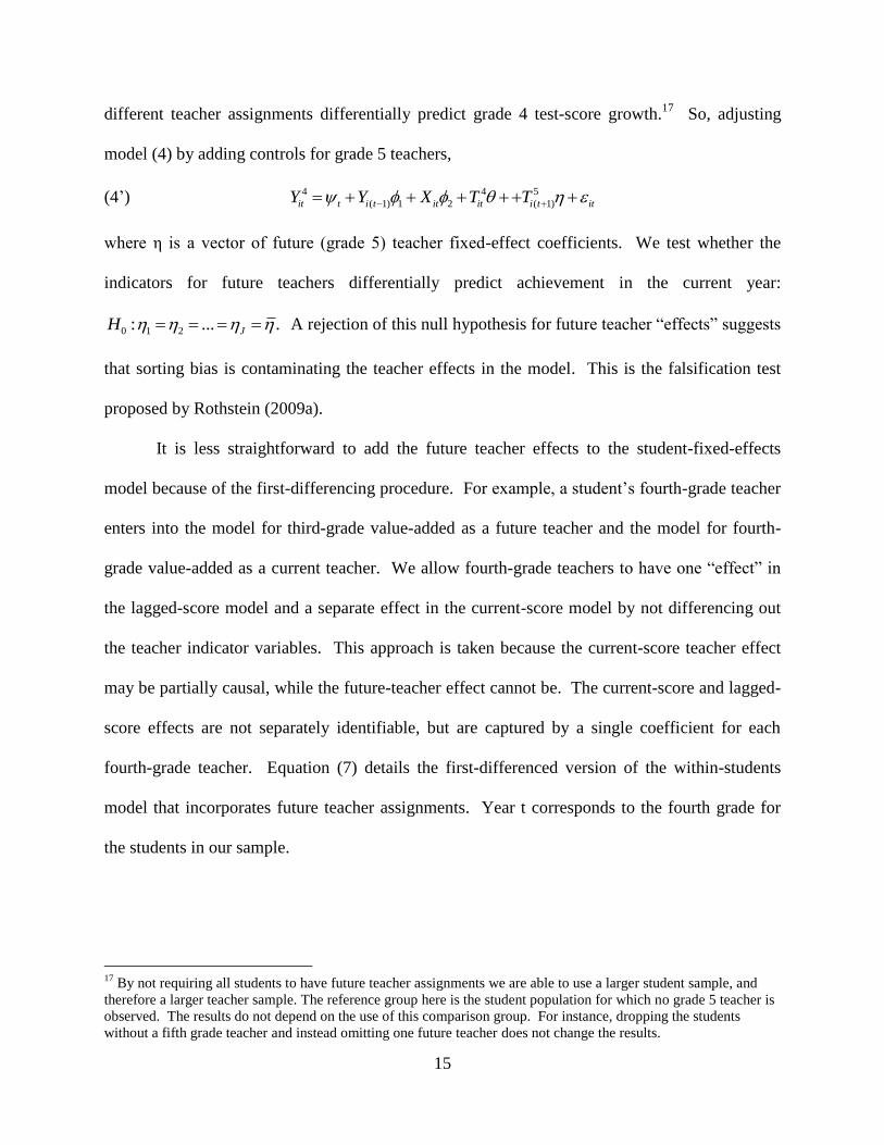
different teacher assignments differentially predict grade 4 test-score growth.17

So, adjusting

model (4) by adding controls for grade 5 teachers,

(4‟) 4 4 5

( 1) 1 2 ( 1)it t i t it it i t itY Y X T T

where η is a vector of future (grade 5) teacher fixed-effect coefficients. We test whether the

indicators for future teachers differentially predict achievement in the current year:

0 1 2: ... .JH A rejection of this null hypothesis for future teacher “effects” suggests

that sorting bias is contaminating the teacher effects in the model. This is the falsification test

proposed by Rothstein (2009a).

It is less straightforward to add the future teacher effects to the student-fixed-effects

model because of the first-differencing procedure. For example, a student‟s fourth-grade teacher

enters into the model for third-grade value-added as a future teacher and the model for fourth-

grade value-added as a current teacher. We allow fourth-grade teachers to have one “effect” in

the lagged-score model and a separate effect in the current-score model by not differencing out

the teacher indicator variables. This approach is taken because the current-score teacher effect

may be partially causal, while the future-teacher effect cannot be. The current-score and lagged-

score effects are not separately identifiable, but are captured by a single coefficient for each

fourth-grade teacher. Equation (7) details the first-differenced version of the within-students

model that incorporates future teacher assignments. Year t corresponds to the fourth grade for

the students in our sample.

17

By not requiring all students to have future teacher assignments we are able to use a larger student sample, and

therefore a larger teacher sample. The reference group here is the student population for which no grade 5 teacher is

observed. The results do not depend on the use of this comparison group. For instance, dropping the students

without a fifth grade teacher and instead omitting one future teacher does not change the results.

16

4 5

( 1) 1 2 3 4 ( 1) 5it i t i t it it it i t itY Y X S T T u

3 4

( 1) ( 1) ( 2) 1 ( 1) 2 ( 1) 3 ( 1) 3 4 ( 1)i t i t i t i t i t i t it i tY Y X S T T u

(7) ( 1) ( 1) ( 1) ( 2) 1 ( 1) 2 ( 1) 3

4 3 5 4

4 ( 1) 3 ( 1) 5 4 ( 1)

( ) ( ) ( ) ( ) ( )

( )

it i t i i t t i t i t it i t it i t

it i t i t it it i t

Y Y Y Y X X S S

T T T T u u

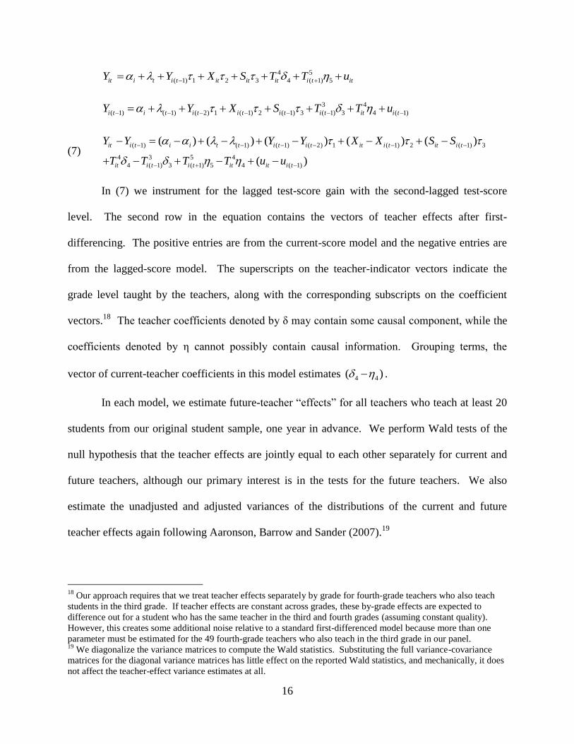
In (7) we instrument for the lagged test-score gain with the second-lagged test-score

level. The second row in the equation contains the vectors of teacher effects after first-

differencing. The positive entries are from the current-score model and the negative entries are

from the lagged-score model. The superscripts on the teacher-indicator vectors indicate the

grade level taught by the teachers, along with the corresponding subscripts on the coefficient

vectors.18

The teacher coefficients denoted by δ may contain some causal component, while the

coefficients denoted by η cannot possibly contain causal information. Grouping terms, the

vector of current-teacher coefficients in this model estimates 4 4( ) .

In each model, we estimate future-teacher “effects” for all teachers who teach at least 20

students from our original student sample, one year in advance. We perform Wald tests of the

null hypothesis that the teacher effects are jointly equal to each other separately for current and

future teachers, although our primary interest is in the tests for the future teachers. We also

estimate the unadjusted and adjusted variances of the distributions of the current and future

teacher effects again following Aaronson, Barrow and Sander (2007).19

18

Our approach requires that we treat teacher effects separately by grade for fourth-grade teachers who also teach

students in the third grade. If teacher effects are constant across grades, these by-grade effects are expected to

difference out for a student who has the same teacher in the third and fourth grades (assuming constant quality).

However, this creates some additional noise relative to a standard first-differenced model because more than one

parameter must be estimated for the 49 fourth-grade teachers who also teach in the third grade in our panel. 19

We diagonalize the variance matrices to compute the Wald statistics. Substituting the full variance-covariance

matrices for the diagonal variance matrices has little effect on the reported Wald statistics, and mechanically, it does

not affect the teacher-effect variance estimates at all.

17

A caveat to the falsification tests in the basic and within-schools models is that they need

not indicate sorting bias. Returning to equation (4‟) and the analogous within-schools model, if

students are sorted into year-(t+1) classrooms based on year-t performance, grade 5 teacher

assignments should be correlated with grade 4 test-score growth. By itself, this is not an

indictment of the value-added model because a model of grade 5 test-score growth, which would

be used to estimate grade 5 teacher effects, would include grade 4 performance as a control.

However, only if grade 4 test scores capture fully differences in academic readiness prior to

grade 5 would this benign explanation for grade 5 teacher effects suffice. If this condition fails,

then the future teacher coefficients in the basic and within-schools models will capture sorting

bias attributable to any unobserved factors that determine both academic performance and

student-teacher assignments. In the context of the models, if the error terms in the basic and

within-schools models are serially correlated, non-zero future teacher effects will be

problematic.20

One way to test the extent to which the future-teacher effects in these models are

capturing bias from sorting on unobservables is to look at prior-year teachers. If lagged test

scores are complete measures of academic readiness, which is the condition required for the

future-teacher effects to be benign, the contributions of prior-year teachers to student

performance should be small. Rothstein (2009a) shows that this is not the case, and in fact

lagged teacher assignments are strong predictors of student outcomes in value-added models.21

This suggests that non-zero future teacher effects in the basic and within-schools models will

reflect sorting bias.

20

We expect that the student fixed effects model will reduce the problem of serial correlation because in the simpler

models the errors will partly reflect omitted student ability and motivation, which are largely unchanging across

grades. 21

We replicate this finding in our data (results available upon request).

18

Turning to the within-students model, the falsification test is a test of strict exogeneity.

By assumption, the time-varying information contained in year-t test scores does not influence

teacher assignments in year-(t+1) in this model. Non-zero future teacher effects indicate that the

future-year teacher assignments are correlated with the first differenced error terms – that is, they

indicate that strict exogeneity fails.

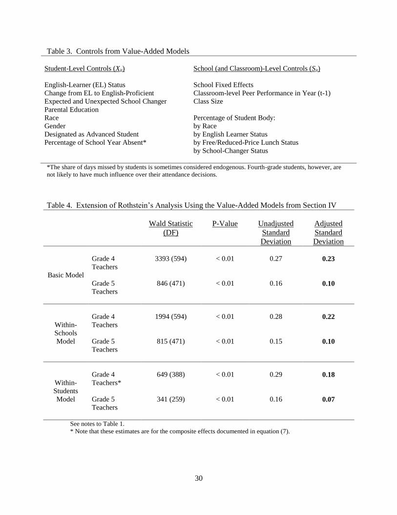
Table 4 details our initial results from the three value-added models - in all three

specifications, the significance of the future-teacher “effects” cannot be rejected. Although the

results in Table 4 continue to show non-zero future teacher effects, note that the estimates of the

standard deviations of teacher effects are much smaller than the analogous estimates in Table 1.

For example, the ratio of the adjusted standard deviation of the future-teacher-effects distribution

to the adjusted standard deviation of the current-teacher-effects distribution falls below one half

in each of the models in Table 4 (down from approximately 0.6 in Table 1).22

Compared to

Table 1, Table 4 indicates that richer value-added models that evaluate teachers over multiple

years reduce the bias in the estimated teacher effects.23

One potentially important aspect of the results in Table 4 is that some of the future-

teacher “effects” are estimated using multiple cohorts of students. If the sorting captured by

Rothstein‟s estimates (and our analogous estimates) is transitory to some extent then using

multiple cohorts of students to evaluate teacher effects will help mitigate the bias. To illustrate,

we write the single-year teacher effect estimate for teacher j at school k in year t from the basic

value-added model as the sum of five components:

22

Note that the meaning of this ratio is less clear in the student-fixed-effects model because the current-teacher

effects from this model estimate the joint parameter 4 4( ) in equation (7). Ultimately, however, the important

result from the student-fixed-effects model is that the future-teacher “effects” have a less predictive power over

current test-score growth. 23

The control variables added to the specifications marginally reduce the sorting bias. This result is consistent with

Rothstein (2009a). Although Rothstein does not report results from models that incorporate student or school-level

control variables, he notes that his results do not qualitatively change if they are included in the model.

19

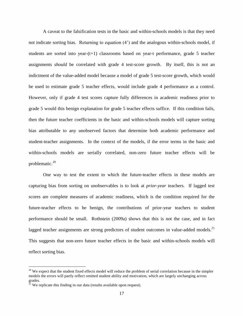
(8) ˆ ( )jkt j k j jt jt

In (8), j is teacher j‟s true effect, k measures the quality of school k, j measures bias from

persistent student sorting to teacher j across years, jt measures bias from non-persistent student

sorting to teacher j and jt is the statistical noise associated with the teacher-effect estimate. If

0k the within-schools model is appropriate. Including additional student-level controls

and/or student fixed effects will reduce the impacts of j and jt ; however, if students are

sorted to teachers based on dynamic and unobserved attributes that are correlated with test-score

growth (e.g., expected mean reversion), these terms can be non-zero in expectation even in the

within-students model.

Using multiple years of data to evaluate teachers will reduce the bias from sorting on

unobservables to the extent that the sorting is transitory and captured by jt rather than j . So

long as student sorting is partly transitory, the variance of our estimated teacher effects will fall

with the number of cohorts observed for each teacher j because jt is being averaged over an

increasing number of cohorts of students. In the extreme, if sorting on unobservables contributes

only to jt (i.e., it is entirely non-persistent from year to year), the sorting bias will go to zero as

t increases.

Table 5 provides compelling evidence that transitory sorting bias may be an important

concern in the data. We group students by year-(t+1) classrooms, then calculate the within-

teacher, across-year correlations of classroom-average year-t gainscores for the year-(t+1)

teachers who teach in each year of the within-students data panel. In the context of equation (8),

for teacher j these correlations provide a rough measure of the relationship between ( )j jt

20

and ( 1)( )j j t . Correlations near one would suggest that there is little scope for transitory

bias, and that adding additional years of teacher data will not be helpful. Correlations near zero

would indicate that the sorting bias can be reduced by evaluating teachers across multiple years.

The first panel of Table 5 reports correlations for raw year-t gainscores, which range between

0.30 and 0.36 across years. The second panel reports correlations for year-t gainscores that are

demeaned within students (i.e., we subtract students‟ average gains), which are even smaller and

range from 0.14 to 0.30. Although these correlations are not zero, they are far from one,

suggesting that transitory sorting bias can be reduced by evaluating teachers across multiple

years.

As a second way to investigate the significance of transitory sorting bias we replicate our

analysis from Table 4 but only evaluate future teachers who teach students in every possible year

of the data panel. For the basic and within-schools models, this means that future teachers teach

students in four consecutive years. For the within-students model, future teachers teach students

in three consecutive years (recall that we only use three year-cohorts of students in the within-

students model).

We report our results in Table 6. Consistent with what is suggested by the correlations in

Table 5, future-teacher “effects” are smaller when we focus on future teachers who teach

multiple cohorts of students. In fact, in the student-fixed-effects model, when we focus on future

teachers who teach at least three classrooms of students, the adjusted variance of grade 5 teacher

effects goes to zero. This suggests that at least some of the sorting bias uncovered by Rothstein

(2009a) is transitory.24

This finding highlights perhaps the most policy-relevant implication of

our study – evaluating teachers over multiple years will improve the performance of value-added

24

Our transitory-sorting bias finding is consistent with other work that finds that multi-year teacher effects are more

stable (McCaffrey et al., 2009) and more predictable (Goldhaber and Hansen, 2009). However, reduced sampling

variance will also be a determinant of these other results.

21

models, and depending on the sorting environment, may be sufficient to mitigate sorting bias if

static tracking is adequately controlled for.25

V. Is this Transitory Sorting Bias or Sample Selection?

In addition to transitory sorting bias, sample selection may also partly explain our results

in Table 6. For example, by requiring teachers to teach in all three years of our data panel, we

exclude a disproportionate share of inexperienced teachers. If students are sorted differently to

experienced and inexperienced teachers, this could contribute to our findings. Although we

cannot capture fully the differences between the teachers who do and do not exit the data panel,

we can replicate the correlative analysis in Table 5 separately for the experienced and

inexperienced teachers who remained in the dataset for all three years. We present these

correlations in Table 7 - they do not suggest that the magnitude of transitory sorting bias will

differ across experienced and inexperienced teachers.26

We also directly test the extent to which our results in Table 6 are driven by sample

selection. If what we‟ve uncovered is a sample-selection effect, then if we remove a cohort of

student data and re-run the model using the new student subsample but the same teachers, the

adjusted variance of grade 5 teacher effects should remain near zero, and the Wald test should

continue to retain the null that all grade 5 teachers have an identical "effect" on grade 4

achievement. Table 8 shows the results when we re-estimate the within-students model after

removing one cohort of grade 4 students at a time. The adjusted variance of grade 5 teachers

25

Although we focus on future teachers, the analysis is also relevant for lagged teachers. In omitted results we find

that the patterns of bias that are associated with transitory sorting for future teachers are also reflected among lagged

teachers, although the interpretation of the lagged-teacher analysis is less straightforward for a handful of reasons,

some specific to our dataset (contact the authors for details). 26

We omit the demeaned-gainscore correlations for brevity - they are smaller in magnitude and display a similar

pattern to the raw gainscores.

22

now rises. Also, in two of three cases the adjusted variance for the grade 4 teachers also

increases as would be expected.

So, why does the fixed-effect model using future teachers who teach in all years, shown

in Table 6, appear to salvage hope for the use of value-added models? We conclude that there is

not something unusual about this sample of grade 5 teachers. Rather, the main reason why we

succeed in reducing future teacher effects to zero has mostly to do with the fact that in Table 6

we include only grade 5 teachers who teach in all years in the data. The use of multiple years of

data reduces transitory sorting bias significantly.27

VI. The Variance of Teacher Quality in San Diego

The results from the previous section suggest that we can estimate the variance of causal

teacher effects in San Diego using a within-students value-added model that focuses on teachers

who teach in all three years of our data panel. For this analysis we return to the within-students

model in equation (6) from Section IV, and estimate teacher effects for fourth-grade teachers.

Unlike in the previous analysis, we do not include future teachers in the model, and estimate a

typical first-differenced specification (as opposed to the non-standard specification in equation

(7)).

Across all of the fourth-grade teachers in our within-students sample, the adjusted

standard deviation of the teacher effects from the model in equation (6) is estimated to be 0.22 –

this number is similar in magnitude to the results above.28

To estimate the magnitude of the

variance of actual teacher quality, free from sorting bias, we split the teacher sample into two

27

In an analysis omitted for brevity, we investigated the extent to which transitory student sorting is exacerbated by

principal turnover. Although our findings are consistent with a principal-turnover effect in the expected direction,

the effect is not statistically significant. One implication of this result is that transitory student sorting does not

unduly depend on principal turnover. Further details are available from the authors upon request. 28

Recall that the within-student teacher “effect” estimates in Tables 6 and 8 are from the non-standard first-

differenced model in equation (7).

23

groups. Group (A) consists of fourth-grade teachers who taught in all three years of our within-

students data panel and group (B) consists of teachers who did not. Approximately 45 percent of

the fourth-grade teachers belong to group (A) and 55 percent to group (B).29

Consistent with the

transitory-sorting-bias result in Table 6, the adjusted variance of the teacher effects from group

(A) is approximately 24 percent smaller than the adjusted variance of the teacher effects from

group (B). Correspondingly, the standard deviations of the adjusted teacher-effect distributions,

measured in standard-deviations of the test, are 0.20 for group (A) and 0.23 for group (B). The

standard deviation of the adjusted difference-in-variance between the two groups is 0.11. Table

9 documents these results.

Although the analysis in the previous section suggests that the observed variance gap

between the teachers in groups (A) and (B) will be driven, at least in part, by differences in

transitory sorting bias, two other explanations merit discussion. First, again, sample selection

may be a concern if group (A) is a more homogeneous group of teachers than group (B). As

shown in Table 10, there are some observable differences in experience and education that

suggest that this might be a concern. Specifically, teachers in group (A) are likely to be more

experienced and to have a master‟s degree. We investigate the extent to which differences across

groups along these dimensions might explain the observed variance difference by estimating the

within-group variance of teacher quality for more and less experienced teachers, and then for

teachers with and without master‟s degrees. The within-group variance of teacher effects among

teachers with master‟s degrees is higher than the within-group variance of those without, which

29

Note that in Table 6, for fifth-grade teachers, roughly 57 percent taught in all three years of the data panel. The

difference in stability between our fourth- and fifth-grade teacher samples may be explained by the different

selection criteria. Our initial sample of fifth-grade teachers in Table 4 teach at least 20 students for whom we

observe teacher assignments in four consecutive years, while our sample of fourth-grade teachers teach at least 20

students for whom we observe teacher assignments in just three consecutive years. Also, the fifth-grade teacher

sample is identified conditional on students being taught by one of the teachers in the fourth-grade teacher sample.

24

works counter to the observed variance gap. For experience, there is more variation among

teachers with 10 or more years of experience and among novice teachers (with 5 or fewer years

of experience) than among teachers with 5-10 years of experience. Ultimately, the variance

decompositions based on grouping teachers by observable qualifications do not suggest a clear

variance-gap effect.30

We also note that the grouping criterion here is somewhat arbitrary in the sense that there

is nothing particularly special about the years covered by our data panel. For example, some of

the teachers in group (A) surely left the district in the year after our data panel ended or didn‟t

teach in the year before it started, and some of the teachers in group (B) surely taught in three or

more contiguous years outside of the data panel (for example, if a teacher taught in the year prior

to the first year of our data panel, and then the first two years of our data panel but not the third,

we would assign the teacher to group (B)).

The second explanation for the observed variance gap is that it occurs by chance. To

evaluate this possibility, we use a bootstrap to derive empirically the distribution from which the

variance-gap estimate would be drawn if the sample were split at random. We randomly assign

the teachers from our sample into two groups that are equivalent in size to groups (A) and (B)

above, and calculate the adjusted-variance gap between these randomly assigned groups. We

repeat this procedure 500 times and use the 500 variance-gap estimates to define the variance-

gap distribution. The variance gap is calculated as the adjusted variance of teacher effects in the

30

The differences in variances across the teacher samples split by observable qualifications are small, in the

neighborhood of 0.01 to 0.02 standard deviations. Although we cannot disentangle the effects of transitory sorting

bias from the observable differences across teachers in the two samples of interest (groups A and B), there is a large

literature showing that teachers differ only mildly in effectiveness based on observable qualifications (Hanushek,

1996; exceptions in the literature include Clotfelter, Ladd and Vigdor, 2007). Perhaps most relevant to the present

study, Betts, Zau and Rice (2003) estimate value-added models in the San Diego Unified School District using

student fixed effects, with separate models for elementary, middle and high school students. Although they find

some evidence that teacher qualifications matter at the high school level, they find very little evidence of this in

elementary schools.

25

smaller group minus the adjusted variance of teacher effects in the larger group, all divided by

the adjusted variance of teacher effects in the larger group. In other words, we calculate

[var( ) var( )] / var( ))GroupA GroupB GroupB . The average variance gap generated by the

bootstrap analysis is +1 percent. The standard deviation in this variance gap is quite large

though, at 24 percent. Thus, the variance gap estimated between the teachers in groups (A) and

(B), -24 percent as shown in Table 9, is just over a standard deviation away from the average of

the empirical variance-gap distribution (at approximately the 13th

percentile of the range of

bootstrapped estimates). Although the empirical variance-gap distribution is wide (the 90-

percent confidence interval ranges from -35 and +45 percent), which limits our ability to detect

statistical significance even when the observed variance gap is large, the gap estimated between

groups (A) and (B) is suggestive of a transitory-sorting-bias effect.

VII. Conclusion

On the one hand, our results corroborate Rothstein‟s key finding that value-added models

of student achievement can produce biased estimates of teacher effects. In fact, we show that

even detailed value-added models that estimate teacher effects across multiple cohorts of

students can still produce biased estimates, as evidenced by the future-teacher “effects”

documented in Tables 4, 6 and 8. However, on the other hand, our results are encouraging

because they indicate that sorting bias in value-added estimation need not be as large as is

implied by Rothstein‟s work. A key finding here is that using multiple years of classroom

observations for teachers will reduce sorting bias in value-added estimates. This result raises

concerns about using single-year measures of teacher value-added to evaluate teacher

effectiveness. For example, one may not want to use achievement gains of the students of novice

26

teachers who are in their first year of teaching to make decisions about which novice teachers

should be retained.

In our setting in San Diego, using a student-fixed-effects model and evaluating teachers

who teach students in three consecutive years mitigates the contribution of sorting-bias to the

teacher-effect estimates. Although this result may not universally generalize, and depends on the

degree of student-teacher sorting in our data, it suggests that under some circumstances value-

added modeling can continue to be a powerful tool in the analysis of teacher effectiveness.

Nonetheless, to the extent that our results corroborate Rothstein‟s findings, they highlight

an important issue with incorporating value-added measures of teacher effectiveness into high-

stakes teacher evaluations. Namely, value-added is manipulable by administrators who

determine students‟ classroom assignments. Our entire analysis is based on a low-stakes

measure of teacher effectiveness. If high stakes were assigned to value-added measures of

teacher effectiveness, sufficient safeguards would need to be put in place to ensure that the

system could not be gamed through purposeful sorting of students to teachers for the benefit of

altering value-added measures of teacher effectiveness.

27

References

Aaronson, Daniel, Lisa Barrow and William Sander. 2007. Teachers and Student

Achievement in the Chicago Public High Schools. Journal of Labor Economics 25:95-135.

Anderson T.W. and Cheng Hsiao. 1981. Estimation of Dynamic Models with Error

Components. Journal of the American Statistical Association. 76:598-609.

Betts, Julian R., Andrew Zau and Lorien Rice. 2003. Determinants of Student Achievement:

New Evidence from San Diego, San Francisco: Public Policy Institute of California.

Downloadable from www.ppic.org.

Clotfelter, Charles T., Helen F. Ladd and Jacob L. Vigdor. 2007. Teacher-Student Matching

and the Assessment of Teacher Effectiveness. Journal of Human Resources. 41:778-820.

Goldhaber, Dan and Michael Hansen. 2008. Is It Just a Bad Class? Assessing the Stability of

Measured Teacher Performance. CRPE Working Paper #2008-5.

Hanushek, Eric, John Kain, Daniel O‟Brien, and Steven Rivkin. 2005. The Market for

Teacher Quality. Working Paper no. 11154, National Bureau of Economic Research,

Cambridge, MA.

Hanushek, Eric. 1996. Measuring Investment in Education. The Journal of Economic

Perspectives 10:9-30.

Harris, Douglas and Tim R. Sass. 2006. Value-Added Models and the Measurement of

Teacher Quality. Unpublished manuscript, Department of Economics, Florida State

University, Tallahassee.

-- 2007. What Makes for a Good Teacher and Who Can Tell? Unpublished manuscript,

Department of Economics, Florida State University, Tallahassee.

Jacob, Brian and Lars Lefgren. 2007. Principals as Agents: Subjective Performance

Assessment in Education. Working Paper no. 11463, National Bureau of Economic

Research, Cambridge, MA.

Kane, Thomas and Douglas Staiger. 2002. The Promise and Pitfalls of Using Imprecise

School Accountability Measures. Journal of Economic Perspectives 16:91-114.

-- 2008. Estimating Teacher Impacts on Student Achievement: An Experimental

Evaluation. Working Paper no. 14607, National Bureau of Economic Research,

Cambridge, MA.

Koedel, Cory (forthcoming). An Empirical Analysis of Teacher Spillover Effects in

Secondary School. Economics of Education Review.

28

Koedel, Cory and Julian R. Betts. 2007. Re-Examining the Role of Teacher Quality in the

Educational Production Function. Working Paper 07-08, University of Missouri, Columbia.

-- (forthcoming). Value-Added to What? How a Ceiling in the Testing Instrument

Influences Value-Added Estimation. Education Finance and Policy.

McCaffrey, Daniel F., J.R. Lockwood, Tim R. Sass and Kata Mihaly. 2009. The Inter-

Temporal Variability of Teacher Effect Estimates. Education Finance and Policy 4.

Murnane, Richard J., Judith D. Singer, John B. Willett, James J. Kemple and Randall J.

Olson. 1991. Who Will Teach? Policies That Matter, Cambridge, MA: Harvard University

Press.

Nye, Barbara, Spyros Konstantopoulos and Larry V. Hedges. 2004. How Large are Teacher

Effects? Educational Evaluation and Policy Analysis 26:237-257.

Podgursky, Michael J. and Mathew G. Springer. 2007. Teacher Performance Pay: A Survey.

Journal of Policy Analysis and Management 26:909-950.

Rockoff, Jonah. 2004. The Impact of Individual Teachers on Student Achievement: Evidence

from Panel Data. American Economic Review, Papers and Proceedings.

Rothstein, Jesse. 2009a (forthcoming). Teacher Quality in Educational Production: Tracking,

Decay, and Student Achievement. Quarterly Journal of Economics.

Rothstein, Jesse. 2009b. Student Sorting and Bias in Value-Added Estimation: Selection on

Observables and Unobservables. Education Finance and Policy 4.

29

Table 1. Standard Deviations of Teacher Effects from a Model with Controls for Past, Current

and Future Teachers. Dependent Variable: Fourth-Grade Gain in Test Score

Wald Statistic (DF)

P-Value Unadjusted Standard

Deviation

Adjusted Standard

Deviation

Grade 4

Teachers

952 (292) <0.01 0.40 0.24

Grade 5

Teachers

610 (253) <0.01 0.30 0.15

The Wald statistics and p-values refer to tests that all teachers in the given grade have identical effects on student

gains in grade 4. The standard deviations refer to the standard deviations of estimated teacher effects, both raw and

adjusted as explained in the text.

Table 2. Average Within-Teacher Standard Deviations of Students‟ Period (t-1) Test Scores Within Schools Across District

Actual Random

Assignment

Perfect

Sorting

Random

Assignment

Perfect

Sorting

Standard Deviations of

Lagged Scores

0.81

0.90

0.32

0.99

<0.01 Note: In the “Perfect Sorting” columns students are sorted by period (t-1) test-score levels in math. For the

randomized assignments, students are assigned to teachers based on randomly generated numbers from a uniform

distribution. The random assignments are repeated 25 times and estimates are averaged across all random

assignments and all teachers. The estimates from the simulated random assignments are very stable across

simulations.

30

Table 3. Controls from Value-Added Models

Student-Level Controls (Xit)

School (and Classroom)-Level Controls (Sit)

English-Learner (EL) Status

Change from EL to English-Proficient

Expected and Unexpected School Changer

Parental Education

Race

Gender

Designated as Advanced Student

Percentage of School Year Absent*

School Fixed Effects

Classroom-level Peer Performance in Year (t-1)

Class Size

Percentage of Student Body:

by Race

by English Learner Status

by Free/Reduced-Price Lunch Status

by School-Changer Status

*The share of days missed by students is sometimes considered endogenous. Fourth-grade students, however, are

not likely to have much influence over their attendance decisions.

Table 4. Extension of Rothstein‟s Analysis Using the Value-Added Models from Section IV

Wald Statistic

(DF)

P-Value

Unadjusted

Standard

Deviation

Adjusted

Standard

Deviation

Basic Model

Grade 4

Teachers

3393 (594)

< 0.01

0.27

0.23

Grade 5

Teachers

846 (471) < 0.01 0.16 0.10

Within-

Schools

Model

Grade 4

Teachers

1994 (594)

< 0.01

0.28

0.22

Grade 5

Teachers

815 (471) < 0.01 0.15 0.10

Within-

Students

Model

Grade 4

Teachers*

649 (388)

< 0.01

0.29

0.18

Grade 5

Teachers

341 (259) < 0.01 0.16 0.07

See notes to Table 1.

* Note that these estimates are for the composite effects documented in equation (7).

31

Table 5. Across-Year Correlations in Year-t Gainscores Averaged at the Teacher-by-Year Level

for Year-(t+1) Teachers Who Taught in all Three Years of the Within-Students Panel.

Raw Gainscores

Year 1 Year 2 Year 3

Year 1 1

Year 2 0.35 1

Year 3 0.30 0.34 1

Year-t Gainscores Demeaned Within Students

Year 1 Year 2 Year 3

Year 1 1

Year 2 0.20 1

Year 3 0.14 0.30 1

Table 6. Extension of Rothstein‟s Analysis Using the Value-Added Models from Section IV and

Only Modeling Future Teachers Who Taught Students in Each Year of the Data Panel

Wald Statistic

(DF)

P-Value

Unadjusted

Variance (sd)

Adjusted

Variance (sd)

Basic Model

Grade 4

Teachers

4640 (594)

< 0.01

0.27

0.23

Grade 5

Teachers

268 (140) < 0.01 0.14 0.09

Within-

Schools

Model

Grade 4

Teachers

2260 (594)

< 0.01

0.28

0.23

Grade 5

Teachers

260 (140) < 0.01 0.14 0.08

Within-

Students

Model

Grade 4

Teachers*

684 (388)

< 0.01

0.29

0.19

Grade 5

Teachers

158 (147) 0.25 0.13 0.00**

Notes: See notes to Table 1. For the basic and within-schools models this analysis includes fifth-grade teachers

who teach in all four years of our data panel. In the within-students model we evaluate just three year-cohorts of

students and therefore we include fifth-grade teachers who teach in three consecutive years.

* Note that these estimates are for the composite effects documented in equation (7).

** Adjusted-variance estimate was marginally negative.

32

Table 7. Across-Year Correlations in Year-t Gainscores Averaged at the Teacher-by-Year Level

for Year-(t+1) Teachers who Taught in all Three Years of the Within-Students Panel, by Teacher

Experience.

Raw Gainscores – Experienced Teachers (N = 104)

Year 1 Year 2 Year 3

Year 1 1

Year 2 0.27 1

Year 3 0.33 0.38 1

Raw Gainscores – Inexperienced Teachers (N = 43)

Year 1 Year 2 Year 3

Year 1 1

Year 2 0.59 1

Year 3 0.22 0.23 1

Table 8. Within-Students Model Using Only Future Teachers Who Taught Students in Each

Year of the Data Panel, With Each of the Three Year Cohorts Individually Omitted from the

Dataset.

Wald Statistic

(DF)*

P-Value

Unadjusted

Variance (sd)

Adjusted

Variance (sd)

Drop Fourth-

Grade

Cohort in

1999-2000

Grade 4

Teachers**

568 (369)

< 0.01

0.31

0.18

Grade 5

Teachers

181 (147) 0.03 0.17 0.06

Drop Fourth-

Grade

Cohort in

2000-2001

Grade 4

Teachers**

651 (374)

< 0.01

0.34

0.21

Grade 5

Teachers

190 (147) 0.01 0.20 0.09

Drop Fourth-

Grade

Cohort in

2001-2002

Grade 4

Teachers**

617 (332)

< 0.01

0.36

0.23

Grade 5

Teachers

196 (147) < 0.01 0.21 0.07

See notes to Table 1. * The number of grade 4 teachers included in the model changes across rows because some of the grade 4

teachers only taught in a single year. Note that the 2001-2002 cohort of students was somewhat larger than the other

two cohorts, which explains why there are fewer grade 4 teachers in the model when this cohort is dropped.

** These estimates are for the composite effects documented in equation (7).

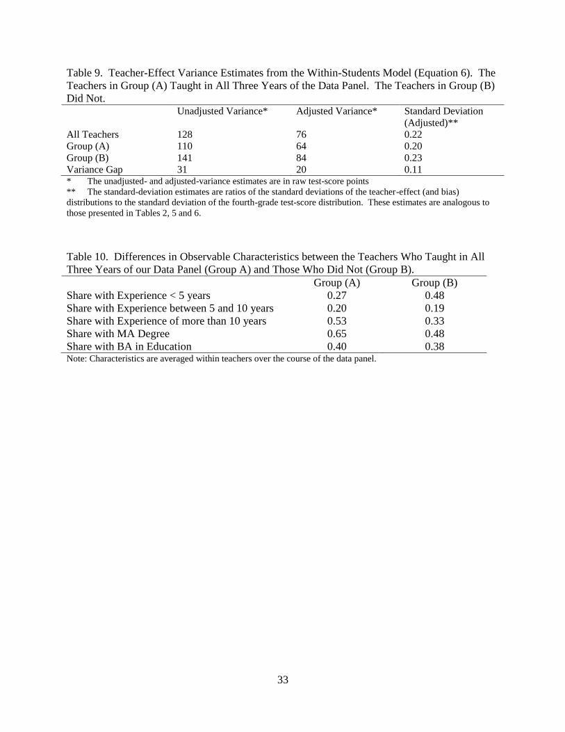
33

Table 9. Teacher-Effect Variance Estimates from the Within-Students Model (Equation 6). The

Teachers in Group (A) Taught in All Three Years of the Data Panel. The Teachers in Group (B)

Did Not. Unadjusted Variance* Adjusted Variance* Standard Deviation

(Adjusted)**

All Teachers 128 76 0.22

Group (A) 110 64 0.20

Group (B) 141 84 0.23

Variance Gap 31 20 0.11 * The unadjusted- and adjusted-variance estimates are in raw test-score points

** The standard-deviation estimates are ratios of the standard deviations of the teacher-effect (and bias)

distributions to the standard deviation of the fourth-grade test-score distribution. These estimates are analogous to

those presented in Tables 2, 5 and 6.

Table 10. Differences in Observable Characteristics between the Teachers Who Taught in All

Three Years of our Data Panel (Group A) and Those Who Did Not (Group B).

Group (A) Group (B)

Share with Experience < 5 years 0.27 0.48

Share with Experience between 5 and 10 years 0.20 0.19

Share with Experience of more than 10 years 0.53 0.33

Share with MA Degree 0.65 0.48

Share with BA in Education 0.40 0.38 Note: Characteristics are averaged within teachers over the course of the data panel.