Does SHEM for Additive Schwarzwork better than predicted by itscondition number estimate ?

Petter E. Bjørstad2, Martin J. Gander1, Atle Loneland2, and TalalRahman3

1 Introduction and Model Problem

The SHEM (Spectral Harmonically Enriched Multiscale) coarse space is anew coarse space for arbitrary overlapping or non-overlapping domain de-composition methods. In contrast to recent new coarse spaces like GenEO[13] or the one in [12] that improve certain Rayleigh quotients in the con-vergence analysis of the underlying domain decomposition method, SHEM isbased on understanding the stationary iterates of the domain decompositionmethod itself (see [6] for details), and can thus be constructed and used alsofor domain decomposition methods which do not (yet) have such a conver-gence analysis, like for example Restricted Additive Schwarz (RAS) [7], oroptimized Schwarz [4]. SHEM is based on the approximation of an optimalcoarse space which was discovered in [3], and further studied in [5, 4, 7], see[6] for a general introduction, and also [9] for the specific case of AdditiveSchwarz (AS). SHEM can use spectral information, as its name indicates,but can also be constructed avoiding eigenvalue problems, for examples, see[8]. If a convergence analysis for the domain decomposition method is avail-able, SHEM can improve the corresponding convergence estimate, see [8] fora condition number estimate when SHEM is used with AS. We are interestedhere to test numerically if in this case

1. the hypothesis of small overlap (one or two mesh sizes) in the proof in [9]is necessary for the condition number estimate to hold in practice;

2. the quadratic growth in the factor H/h in the condition number estimatefrom [9] is really present when the method is used numerically.

Section of Mathematics, University of Geneva, 1211 Geneva 4, SwitzerlandMartin.Gander@unige.ch · Department of Informatics, University of Bergen, 5020

Bergen, Norway Atle.Loneland@ii.uib.no · Department of Computing, Mathematicsand Physics, Western Norway University of Applied Sciences, 5063 Bergen, Norway

Talal.Rahman@hvl.no

1

2 Petter E. Bjørstad, Martin J. Gander, Atle Loneland, and Talal Rahman

We consider as our model problem the following variational formulation of asecond order elliptic boundary value problem with Dirichlet boundary con-ditions: find u ∈ H1

0 (Ω) such that

a(u, v) =

∫Ω

α(x)∇u · ∇v dx =

∫Ω

fv dx ∀v ∈ H10 (Ω), (1)

where Ω is a bounded convex domain in R2, f ∈ L2(Ω) and α ∈ L∞(Ω) suchthat α ≥ α0 for some positive constant α0. Discretizing this problem using P1finite elements from the finite element space Vh with associated mesh Th(Ω)leads to the linear system

Au = f . (2)

Let Ω be partitioned into non-overlapping open, connected Lipschitz poly-topes Ωi : i = 1, . . . , N such that Ω =

⋃Ni=1Ωi, where each Ωi is assumed

to consist of elements from Th(Ω). We assume that this partitioning is shape-regular. By extending each subdomain Ωi with a distance δ in each direction,we create a further decomposition of Ω into overlapping subdomains Ω′iNi=1.As usual, we assume that each point x ∈ Ω is contained in at most N0 sub-domains (finite covering). The layer of elements in Ωi touching the boundary∂Ωi is denoted by Ωhi and we assume that the triangles corresponding to thislayer are shape regular with minimum diameter hi := min

K∈Th(Ωhi )hK , where hK

is the diameter of the triangle K. The interfaces between two subdomains,Ωi and Ωj , are defined as Γ ij := Ωi ∩ Ωj . The sets of vertices of elementsin Th(Ω) (nodal points) belonging to Ω, Ωi, ∂Ω, ∂Ωi and Γij are denotedby Ωh, Ωih, ∂Ωh, ∂Ωih and Γijh. With each interface we define the space offinite element functions restricted to Γij and zero on ∂Γij as V 0

h (Γij).We define the restriction of the bilinear form a(·, ·) to an interface Γij

shared by two subdomains as

aΓij(u, v) :=

(α|Γij

(x)Dτu,Dτv)L2(Γij)

,

where α|Γij(x) := lim

y∈Ωi→xα(y) and Dτ denotes the tangent derivative with

respect to Γij . In order to obtain continuous basis functions across subdomaininterfaces, we define a second bilinear form on each interface Γij ,

aΓij(u, v) := (αij(x)Dτu,Dτv)L2(Γij)

,

where αij is taken as the maximum of α|Γijand α|Γji

.

Given a partition of unity χiNi=1 subordinate to the overlapping decom-position defined above and corresponding restriction matrices Ri, as well asa suitable coarse space V0 with restriction operator R0, the two-level additiveSchwarz method may be defined for i = 0, . . . N as

Does SHEM for Additive Schwarz work better than predicted? 3

M−1AS,2 =

N∑i=0

RTi A−1i Ri where Ai := RiAR

Ti . (3)

Classically, coarse spaces for Additive Schwarz methods consist of finite ele-ments on a coarser triangulation TH of Ω. This type of choice for the coarsespace, however, is not robust with respect to large variations in the coefficientα.

2 The SHEM Coarse Space

SHEM is based on enriching a particular underlying coarse space, which inthe case of high contrast problems is the multiscale finite element coarsespace, see [1, 10]. We use the variant that generates the multiscale elementsby solving lower dimensional problems along the edges, and then extend-ing the result harmonically into the interior of the element. In the case ofLaplace’s equation on a rectangular domain decomposition, this underlyingcoarse space would just be Q1 finite elements on the subdomains, see [5]. Notethat SHEM is also interesting in this case, since it systematically improvesthe overall convergence of the underlying domain decomposition method inan optimized way, see [9]. We choose here for SHEM a harmonic enrichmentbased on solutions of local eigenvalue problems along the interfaces betweensubdomains1:

Definition 1 (Generalized Interface Eigenvalue Problem). For eachinterface Γij , we define the generalized eigenvalue problem: find ψ and λ,such that

aΓij (ψ, v) := λbΓij (ψ, v) ∀v ∈ V 0h (Γij), (4)

where bΓij (ψ, v) := h−1i∑

k∈Γijh

βkψkvk and βk =∑

K∈Th(Ω)k∈dof(K)

αK .

We will test the following two types of SHEM coarse spaces:

• SHEMm, where m is an integer: here we choose the m eigenfunctionsassociated with the smallest m eigenvalues of (4), and extend each of themharmonically into the two subdomains Ωi and Ωj adjacent to the interfaceΓij with zero Dirichlet boundary conditions on the remaining part of thesubdomain boundaries. These functions are then added to the underlyingmultiscale coarse space to form SHEMm.

• SHEMτ , where τ is a given tolerance: here we choose adaptively on each in-terface Γij to include all eigenfunctions associates with eigenvalues smaller

1 Any other Sturm Liuville problem could be used as well to get a different variant ofSHEM, for example more expensive Schur complements corresponding to the Dirichlet to

Neumann maps [11], or one could construct even cheaper interface basis functions without

eigenvalue problem, see [8].

4 Petter E. Bjørstad, Martin J. Gander, Atle Loneland, and Talal Rahman

than τ , extend them harmonically like above and add them to the under-lying multiscale coarse space to form SHEMτ .

Theorem 1 (Condition Number Estimate [8]). If the overlap is one ortwo mesh sizes, then the condition number of the two level Schwarz operator(3) with the SHEMm coarse space can be bounded by

κ(M−1AS,2A) C20 (N0 + 1), (5)

where C20 '

(1 + 1

λm+1

)and λm+1 := min

imin

Γij⊂∂Ωi

λijmij+1.

The restriction on the overlap size is necessary in the proof based on theabstract Schwarz framework. The convergence estimate in Theorem 1 alsoindicates a quadratic dependence of the condition number on the mesh ratioH/h, even for the case without enrichment, because the inverse of the smallesteigenvalues of (4) have a quadratic dependence on the ratio H/h. In the caseof Laplace’s equation and without enrichment, such that our coarse spaceis just the normal Q1 coarse space, standard domain decomposition theorysays that the condition number of additive Schwarz should depend linearlyon the mesh ratio H/h. We investigate now numerically if these restrictionsare really also properties of SHEMm, or just artefacts in the analysis.

3 Numerical Investigation of the SHEM coarse space

We solve problem (1) with f = 1 on a unit square domain Ω = (0, 1)2, and thecoefficient α(x) represents various (possibly discontinuous) distributions. Weuse AS with SHEMm as a preconditioner for the conjugate gradient method,and stop the iteration when the l2 norm of the residual is reduced by a factorof 10−6. If not stated otherwise, the coefficient α(x) is equal to 1 for all thenumerical examples, except in the areas marked with red where the value ofα(x) is equal to α. All the experiments were carried out using Matlab 9.0 ona serial workstation. For the interface eigenvalue problems, we have in ourimplementation exploited the fact that we are able to extract exactly the 1Dstiffness and mass matrix corresponding to the bilinear forms in Definition 1algebraically from the global problem.

3.1 Is small overlap necessary for SHEM?

We start by studying the dependence on the overlap for the contrast func-tion α(x) shown in Figure 1. For the case of overlap δ = 2h and δ = 8h,we show the iteration counts and condition number estimates in Table 1 for

Does SHEM for Additive Schwarz work better than predicted? 5

Fig. 1 Distribution of α for a geometry with h = 1128

, H = 16h. The regions marked with

red are where α has a large value α.

the classical multiscale coarse space (MS), SHEMm and the adaptive variantSHEMτ=6e−3. We see that even though the theory only addressed small over-lap, SHEMm works very well also with larger overlap, and overlap improvesthe performance like usual. We even see that independence of the contrastarrives for the large overlap already with two enrichment functions instead ofthree. This is because the middle of the three channels crossing the interfacesin Figure 1 is shorter, and for the large overlap case included in the overlap,and thus not a convergence problem any more for the underlying AS; thereare therefore only two channels left the coarse space has to treat, see [6] pre-sented at this conference. In the current adaptive variant SHEMτ=6e−3 it isnot clear how to take into account the overlap, and thus the same number of

MS SHEM1 SHEM2 SHEM3 SHEM4 SHEMτ=6e−3

dim. 49 161 273 385 497

α #it. (κ) #it. (κ) #it. (κ) #it. (κ) #it. (κ) #it. (κ) dim.

100 21 (1.29e1) 16 (7.45e0) 15 (5.99e0) 13 (5.19e0) 13 (5.15e0) 21 (1.29e1) 49102 122 (3.74e2) 70 (1.17e2) 47 (6.70e1) 19 (6.77e0) 16 (5.66e0) 25 (1.10e1) 233

104 367 (3.64e4) 248 (1.10e4) 187 (6.22e3) 19 (6.78e0) 17 (5.73e0) 25 (1.09e1) 233

106 610 (3.64e6) 423 (1.10e6) 290 (6.22e5) 19 (6.78e0) 17 (5.73e0) 25 (1.09e1) 233

100 16 (5.57e0) 15 (4,88e0) 15 (4.82e0) 15 (4.94e0) 15 (4.95e0) 16 (5.47e0) 49102 47 (4.08e1) 28 (1.53e1) 19 (5.58e0) 18 (5.02e0) 18 (4.99e0) 21 (6.26e0) 233104 145 (3.48e3) 55 (1.08e3) 20 (6.03e0) 18 (5.06e0) 18 (4.99e0) 21 (6.55e0) 233

106 241 (3.48e5) 78 (1.08e5) 20 (6.03e0) 18 (5.06e0) 18 (4.99e0) 21 (6.56e0) 233

Table 1 Top half: overlap δ = 2h. Bottom half: overlap δ = 8h. Iteration count and con-dition number estimate for the channel distribution in Figure 1 for the classical multiscale

coarse space, SHEMm, m = 1, 2, 3, 4 and SHEMτ=6e−3 for h = 1128

, H = 16h. Here ’dim’denotes the dimension of the coarse space.

6 Petter E. Bjørstad, Martin J. Gander, Atle Loneland, and Talal Rahman

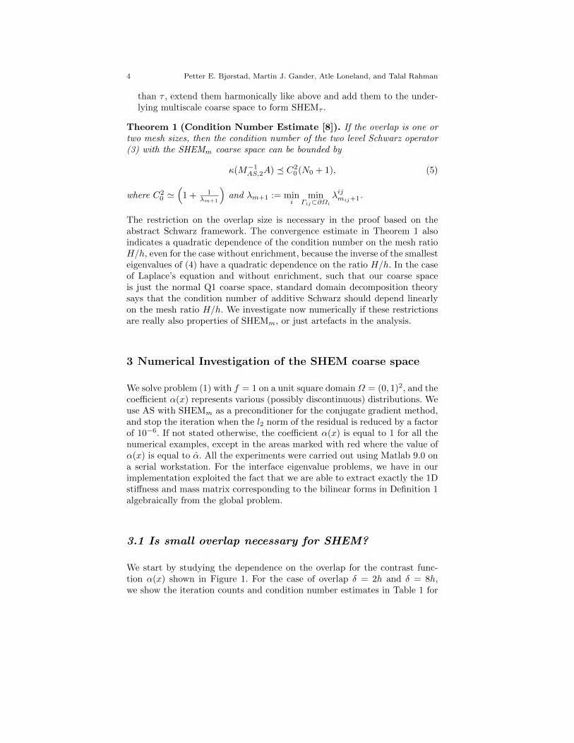
Fig. 2 Distribution of α for a geometry with h = 1128

, H = 16h. The regions marked withred are where α has a large value α.

enrichment functions was chosen. Larger overlap can however also be takeninto account by a different construction of SHEM for AS, see [9].

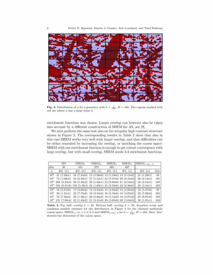
We next perform the same test also on the irregular high contrast structureshown in Figure 2. The corresponding results in Table 2 show that also inthis case SHEM works very well with larger overlap, and that difficulties canbe either remedied by increasing the overlap, or enriching the coarse space:SHEM with one enrichment function is enough to get robust convergence withlarge overlap, but with small overlap, SHEM needs 2-3 enrichment functions.

MS SHEM1 SHEM2 SHEM3 SHEM4 SHEMτ=6e−3

dim. 49 161 273 385 497

α #it. (κ) #it. (κ) #it. (κ) #it. (κ) #it. (κ) #it. (κ) dim.

100 21 (1.29e1) 16 (7.45e0) 15 (5.99e0) 13 (5.19e0) 13 (5.15e0) 21 (1.29e1) 49102 72 (1.09e2) 53 (6.49e1) 27 (1.52e1) 22 (9.47e0) 20 (6.45e0) 36 (2.14e1) 165

104 288 (9.43e3) 98 (5.46e3) 29 (1.60e1) 23 (9.60e0) 21 (6.54e0) 38 (2.44e1) 169106 524 (9.41e6) 156 (5.49e5) 32 (1.60e1) 24 (9.59e0) 22 (6.28e0) 39 (2.44e1) 169

100 16 (5.57e0) 15 (4,88e0) 15 (4.82e0) 15 (4.94e0) 15 (4.95e0) 16 (5.47e0) 49102 29 (1.31e1) 22 (7.75e0) 19 (5.54e0) 18 (5.10e0) 18 (5.05e0) 22 (7.89e0) 165

104 72 (7.56e2) 28 (1.36e1) 20 (5.68e0) 19 (5.12e0) 19 (5.07e0) 25 (9.97e0) 169106 121 (7.50e4) 32 (1.43e2) 21 (5.41e0) 20 (5.05e0) 20 (5.02e0) 26 (1.01e1) 169

Table 2 Top half: overlap δ = 2h. Bottom half: overlap δ = 8h. Iteration count and

condition number estimate for the distribution in Figure 2 for the classical multiscale

coarse space, SHEMm, m = 1, 2, 3, 4 and SHEMτ=6e−3 for h = 1128

, H = 16h. Here ’dim’denotes the dimension of the coarse space.

Does SHEM for Additive Schwarz work better than predicted? 7

MS SHEM1 SHEM2 SHEM3 SHEM4Hh

#it. (κ) #it. (κ) #it. (κ) #it. (κ) #it. (κ)

8 18 (7.67e0) 14 (5.36e0) 14 (5.02e1) 14 (5.07e0) 13 (5.12e0)

16 21 (1.29e1) 16 (7.45e0) 15 (5.99e0) 13 (5.19e0) 13 (5.15e0)

32 29 (2.37e1) 20 (1.22e1) 18 (8.97e5) 15 (7.52e0) 14 (6.55e0)64 41 (4.52e1) 26 (2.23e1) 22 (1.56e1) 19 (1.32e1) 18 (1.03e1)

128 58 (8.85e1) 36 (4.25e1) 30 (2.88e1) 25 (2.23e1) 23 (1.82e1)

256 80 (1.75e2) 50 (8.83e1) 41 (5.57e1) 34 (4.24e1) 31 (3.42e1)

16 367 (3.64e4) 248 (1.10e4) 187 (6.78e3) 19 (6.78e0) 17 (5.73e0)

32 525 (7.47e4) 326 (2.32e4) 252 (1.32e4) 22 (9.33e0) 19 (7.74e0)64 740 (1.51e5) 458 (4.76e4) 329 (2.72e4) 28 (1.70e1) 22 (1.25e1)128 1062 (3.05e5) 665 (9.62e4) 457 (5.52e4) 38 (3.15e1) 29 (2.25e1)

256 1522 (6.12e5)∗ 980 (1.94e5)∗ 679 (1.11e5)∗ 52 (6.06e1) 41 (4.28e1)

16 288 (9.43e3) 98 (5.46e3) 29 (1.60e1) 23 (9.60e0) 21 (6.54e0)32 443 (1.97e4) 129 (1.14e4) 38 (2.75e1) 28 (1.53e0) 23 (8.00e0)64 612 (4.03e4) 170 (2.31e4) 51 (5.07e1) 36 (2.73e1) 29 (1.27e1)

128 856 (8.17e4) 232 (4.65e4) 70 (9.82e1) 48 (5.20e1) 38 (2.26e1)256 1207 (1.64e5) 315 (9.33e4) 98 (1.94e2) 66 (1.02e2) 52 (4.30e1)

* Stagnation.

Table 3 Top: α = 1. Middle: Distribution of α from Figure 1 with α = 104. Bottom:

Distribution of α from Figure 2 with α = 104. Iteration count and condition numberestimate for the classical multiscale coarse space and SHEMm, m = 1, 2, 3, 4, solving

Problem 1 for decreasing h, H = 18

and overlap δ = 2h.

3.2 What is the condition number growth in H/h?

We now test numerically the dependence on the mesh ratio H/h for the casewhere α = 1 and for the high contrast cases given in Figure 1 and 2 withα = 104. The iteration counts and condition number estimates are givenin Table 3 for decreasing h while the subdomain diameter is kept fixed atH = 1/8. We clearly see that the convergence rate is linearly dependenton the mesh ratio H/h, for both the constant coefficient case and the highcontrast cases. This confirms that the restrictions in the analysis in [9] arenot a property of SHEM itself, but rather restrictions of the analysis. We alsosee that for very high contrast, SHEM can even fix stagnation when usingthe appropriate amount of enrichment.

4 Conclusions

The numerical experiments we presented indicate that the first convergenceestimate for SHEM in Theorem 1 might not need the technical assumptionof small overlap, and also that the convergence bound with the square de-pendence on the mesh ratio H/h is too pessimistic. Another important ob-servation is that the dimension of the coarse space is not larger than the

8 Petter E. Bjørstad, Martin J. Gander, Atle Loneland, and Talal Rahman

dimension of the largest subdomain in our experiments, and thus the coarsespace solve remains less expensive than the subdomain solves. Based on thisnumerical investigation, we are currently carefully studying the technical es-timates in the proof of Theorem 1 to see under which conditions on the highcontrast parameter α the overlap restriction and the quadratic dependenceon the mesh ratio in the condition number estimate can be removed. We arealso working on the extension to three dimensional problems, see [2], and ona parallel implementation.

References

1. Jørg Aarnes and Thomas Y. Hou. Multiscale domain decomposition methods forelliptic problems with high aspect ratios. Acta Math. Appl. Sin. Engl. Ser., 18(1):63–

76, 2002.

2. Erik Eikeland, Leszek Marcinkowski, and Talal Rahman. Overlapping Schwarz Meth-ods with Adaptive Coarse Spaces for Multiscale Problems in 3D. arXiv:1611.00968,

November 2016.

3. Martin J Gander and Laurence Halpern. Methodes de decomposition de domaine.Encyclopedie electronique pour les ingenieurs, 2012.

4. Martin J. Gander, Laurence Halpern, and Kevin Santugini Repiquet. Discontinuouscoarse spaces for DD-methods with discontinuous iterates. In Domain Decomposition

Methods in Science and Engineering XXI, pages 607–615. Springer, 2014.

5. Martin J. Gander, Laurence Halpern, and Kevin Santugini Repiquet. A new coarsegrid correction for RAS/AS. In Domain Decomposition Methods in Science and En-

gineering XXI, pages 275–283. Springer, 2014.

6. Martin J. Gander, Laurence Halpern, and Kevin Santugini Repiquet. On optimalcoarse spaces for domain decomposition and their approximation. In these proceedings

(submitted). 2017.

7. Martin J. Gander and Atle Loneland. SHEM: An optimal coarse space for RAS andits multiscale approximation. In Domain Decomposition Methods in Science and En-

gineering XXIII. Springer, 2016.

8. Martin J Gander, Atle Loneland, and Talal Rahman. Analysis of a new harmonicallyenriched multiscale coarse space for domain decomposition methods. arXiv preprint

arXiv:1512.05285, 2015.

9. Martin J. Gander and Bo Song. Complete, optimal and optimized coarse spaces forAS. In these proceedings (submitted). 2017.

10. I. G. Graham, P. O. Lechner, and R. Scheichl. Domain decomposition for multiscalePDEs. Numer. Math., 106(4):589–626, 2007.

11. A. Heinlein, A. Klawonn, J. Knepper, and O. Rheinbach. Multiscale coarse spaces foroverlapping Schwarz methods based on the ACMS space in 2d. ETNA, page submitted,2017.

12. Axel Klawonn, Patrick Radtke, and Oliver Rheinbach. Feti-dp methods with an adap-

tive coarse space. SIAM Journal on Numerical Analysis, 53(1):297–320, 2015.13. Nicole Spillane, Victorita Dolean, Patrice Hauret, Frederic Nataf, Clemens Pechstein,

and Robert Scheichl. Abstract robust coarse spaces for systems of PDEs via generalizedeigenproblems in the overlaps. Numerische Mathematik, 126(4):741–770, 2014.