Does semi-formal credit help to cope ... - uni-heidelberg.de · the feature that credit supply in...

Does semi-formal credit help to cope with aggregate shocks?

Evidence from Roscas and the Indian Ocean Tsunami

Kristina Czura, Stefan Klonner

Goethe University Frankfurt, Germany

August 2, 2010

Abstract

We analyze the e¤ects of the 2004 Indian Ocean Tsunami on credit demand in

Rotating Savings and Credit Associations (Roscas) in South India. We combine �nancial

data from a semi-formal intermediary with geophysical data on the Tsunami. Exploiting

the feature that credit supply in Roscas is �xed on the short term, we estimate the

extent to which the price of credit changed in response to this shock. Comparing

branches a¤ected and una¤ected by the Tsunami before and after the Tsunami hit, we

�nd a signi�cant increase in the interest rate by 5.3 per cent on average in the a¤ected

branches. Interest rates increased most dramatically in the �rst three months after

the Tsunami hit and decreased subsequently over the year 2005. We conclude that (i)

funds provided by Roscas did play a role for coping with this huge negative shock, (ii)

repercussions of the Tsunami in the Rosca credit market were limited in terms of the

order of magnitude of e¤ects, and (iii) semi-formal credit and o¢ cial aid appear to be

substitutes as disaster coping mechanisms rather than complements.

Keywords: Natural Disaster, Roscas, Coping Strategies

JEL categories: O16, Q54

1

1 Introduction

Over the last two decades a body of research on the vulnerability of the poor has accumu-

lated in development economics. Policy makers and researchers alike increasingly recognize

that not only the average level of household income at a given point in time, but also

the ability or inability to cope with income shocks matters for the welfare of the poor.

Townsend�s (1994) seminal study on mutual insurance and consumption smoothing in re-

sponse to income shocks using household survey data has led to further work on particular

mechanisms through which households insure or smooth consumption. Both formal and

informal credit have been identi�ed as important mechanisms in dealing with idiosyncratic

shocks. (e.g. Eswaran & Kotwal (1989); Udry (1990); Udry (1994); Gertler et al. (2002);

Skou�as (2003)). Further, access to credit has been identi�ed to reduce the use of other

coping mechanisms like child labor and reduction of educational attainment of children in

the face of negative income shocks (e.g. Jacoby & Skou�as (1997); Beegle et al. (2006);

Guarcello (2009)).

There is, however, little research on how households cope with large aggregate shocks,

like natural disasters, and what role credit plays in this context. A few studies elicit a

substitution e¤ect of other coping mechanisms like child labor or educational attainment

and credit in the face of aggregate shocks (e.g. Jacoby & Skou�as (1997); Gitter & Barham

(2007)). Sawada (2008) �nds direct evidence for consumption smoothing after the Kobe

earthquake for households having access to credit compared to credit constrained house-

holds. Nevertheless, there is little evidence on the direct use of credit as insurance against

aggregate shocks in the literature. Notable contributions of Del Ninno et al. (2003) and

Khandker (2007) are based on the 1998 �ood in Bangladesh, and �nd that household bor-

rowing, especially informal credit and micro credit, played a major role for consumption

smoothing in the face of this shock.

Very little continues to be known on the e¤ect of large, aggregate shocks on the markets

relevant for households�ability to cope with such risks. Important issues like how e¤ec-

tively credit �ows from regions less a¤ected by a natural disaster to more a¤ected regions,

2

or whether �within a¤ected regions � funds �ow from less to more a¤ected households,

remain largely unexplored. In this paper, we tackle this latter issueby investigating the

consequences of the 2004 Tsunami on an important segment of the credit market in South

India. Using data from a semi-formal �nancial intermediary, we estimate the extent to

which the price of credit changed in response to the Tsunami hit. As the supply of funds is

�xed in the short run in the institution that we study, an increase in the price of credit in

locations a¤ected by the Tsunami allows us to conclude that semi-formal credit was indeed

a relevant coping mechanism. Second, the longitudinal dimension of our data allows us to

identify the dynamics of the role of credit in the aftermath of this large shock.

We use data from 14 branches of a �nancial company in the Indian state of Tamil

Nadu on over 16,000 loans handed out in 2004 and 2005 to address these issues empirically.

The �nancial institution considered are formally organized Roscas (Rotating Savings and

Credit Associations) in which individuals get together to borrow and save. Those Roscas

are administered by the same �nancial company in branches in various locations across the

state of Tamil Nadu. The interest rate for each loan is determined by concurrent competitive

bidding. This feature together with the �xed supply of funds in the short run makes this

institution ideal to test for instantaneous changes in credit demand. In this quasi-natural

experiment, we use di¤erence-in-di¤erence estimation methods to identify changes in the

borrowing interest rate in a¤ected locations relative to una¤ected locations around the hit

of the Tsunami on December 26, 2004. We use geophysical data by Maheshwari et al.

(2005) and Narayan et al. (2005) to capture the extent of the Tsunami hit. Information

on the local severity of the Tsunami from these sources is combined with spatially mapped

Rosca data using GIS methods.

We �nd a signi�cant increase in the interest rate in the a¤ected branches after the

Tsunami. In branches classi�ed as a¤ected, interest rates increased by around 5% on av-

erage. This translates to an increase of around one percentage point relative to an average

borrowing rate of roughly 20%. Accounting for variation in the intensity of the Tsunami

we �nd an increase in the interest rate of around 3% per additional meter of wave height.

3

We conclude, �rst, that funds provided by Roscas did play a role for coping with this

huge negative shock, second, that the repercussions of the Tsunami in the Rosca credit

market were limited in terms of the order of magnitude of e¤ects, and third, that credit

demand increased most dramatically right after the shock. This latter observation is in line

with qualitative evidence on aid �ows and relief programs which are reported to have reached

the a¤ected areas with a time lag of several months. In this connection, our results suggest

that semi-formal credit and o¢ cial aid are substitutes as disaster coping mechanisms, rather

than complements.

The paper is organized as follows. Section 2 takes a closer look at the functioning of

Roscas and the data. In section 3 we describe the identi�cation strategy and estimation

approach. The estimation results are presented in section 4. Robustness checks and some

extensions of the analysis are considered in section 5. Section 6 concludes.

2 Background and Data Description

Tsunami - Geophysical Data

The December 26, 2004 earthquake in Sumatra, Indonesia, caused Tsunami waves to hit

the coast of India. The giant Tsunami waves of 3 to 11 meters in height penetrated in-

land up to 3 km leading to extensive damage in the states of Andhra Pradesh, Kerala,

Tamil Nadu and the Union Territory of Pondicherry on the Indian mainland. The coast of

Tamil Nadu was hit especially hard, accounting with 7995 dead people for over 60% of lost

lives during the Tsunami in India. 230 villages and 418 kuppams (hamlets) were �attened

completely and more than 470,000 people had to evacuate from their homes. Additionally,

the Tsunami caused massive destruction to infrastructure, soil quality, and property, like

boats and �shing equipment, depleting physical capital and productive assets. Fishery and

related activities such as �sh marketing, �sh transport, �sh processing, boat making and

repair is an important economic activity along the coast of Tamil Nadu. Fishermen mostly

living in huts close to the coast were most severely a¤ected in destruction of livelihood.

4

Additionally, they su¤ered from a substantial destruction on production assets with 16,772

boats fully and 19,305 boats partly damaged. Other sources of livelihood along the coast

like agriculture and livestock were a¤ected by loss of 16,083 cattle and in storage of agricul-

tural produce as well as soil destruction or salinization of 8460.24 hectares of agricultural

land and 669.82 hectares of horticultural land. The total value of damage caused to boats,

infrastructure like ports, roads, electricity installations, and water supply, public buildings

and soils is estimated at 2,350,950,000,000 Indian Rupees (AsianDevelopmentBank (2005);

Maheshwari et al. (2005); Narayan et al. (2005); Athukorala & Resosudarmo (2005);

TamilNaduGovernment (2005)).

The extend of damage varied with Tsunami intensity.1 The intensity depends on the

maximum height of the Tsunami waves which themselves are depending on geographic and

geologic conditions. For instance mangrove swamps or the Sri Lankan mainland cushioned

the impact of the waves on parts of the Indian coast. Figure 1 shows the Tsunami intensity

measured at di¤erent geographic points in a survey shortly after the Tsunami. The higher

the Tsunami intensity at a geographic site, the more severely is the destruction at the

hit location (Papadopoulos & Imamura (2001)). For the Tsunami measures we take data

from a survey conducted by the Department of Earthquake Engineering, Indian Institute

of Technology, Roorkee. The data set contains geo codes of Tsunami hit locations and

measures of the run up height and inundation distance at the Tsunami survey measure

points (Maheshwari et al. (2005); Narayan et al. (2005)). The run up height ranges from

1There are di¤erent ways to measure the size of a Tsunami aiming at a common scale for Tsunamis

like the Richter scale for the quanti�cation of earthquakes. One common measure is the Tsunami intensity

depending on the so called run up height. The run up height is the maximum height of the water observed

above a reference sea level. A very common de�nition of the Tsunami intensity is based on Soloviev�s

(1970) calculations as intensity i=log2(p2* run up height) which is also used by the National Geophysical

Data Center (NGDC). Another intensity scale was introduced by Shuto (1993) as intensity i=log2(run up

height). Papadopoulos and Imamura (2001) relate Shuto�s intensity scale based on physical parameters to

their proposed 12 step intensity scale based on observed destruction from a Tsunami. For simpli�cation we

apply a small transformation and use the natural log of the run up height as a measure of tsunami intensity

in the later analysis.

5

3 to 11 meters averaging 5.8 meters in a¤ected areas considered in our study (Table 1).The

sample mean of the run up height corresponds to 2.59 meters. In addition to the physical

run up height we use two measures for the Tsunami intensity. The �rst alternative measure

is the wave intensity formed by the natural log of the run up height as wave intensity =

ln(run up heigth). This is comparable to other measures of Tsunami intensity based on

physical parameters of the Tsunami. Average wave intensity is 1.65 in a¤ected branches

and 0.74 in the whole sample.

The second measure is the damage intensity. We apply the Tsunami intensity mapping in

Tamil Nadu from Narayan et al. (2006). It is formed according to the 12 step intensity scale

by Papadopoulos & Imamura (2001) based on observable destruction caused by a Tsunami.

It ranges from an intensity in step 1 "I. Not felt" to "XII. Completely devastating" in step

12.2 In a¤ected branches the damage intensity ranges from 6.5 corresponding to the category

"damaging" to a damage intensity of 10 corresponding to the category "very destructive"

on the 12 step intensity scale. The average damage intensity in a¤ected branches is nearly

8 representing the category "heavy damaging". The sample mean of the damage intensity

is 3.6.

Chit Fund - Financial Data

We combine the geophysical data with �nancial data from a semi-formal �nancial institu-

tion in the southern Indian state of Tamil Nadu that organizes Roscas. In a Rosca, or chit

fund as they are called in India, a group of people get together regularly to borrow and save.

At each meeting, every member of the group contributes a �xed amount to a common pot

that is allocated to one of the participants. Every participant receives the pot once during

the course of a Rosca. In our study the pot is allocated by an oral ascending bid auction

where the highest bidder receives the pot less the winning bid amount. Once a participant

2The 12 step Intensity scale is: I) Not felt, II) Scarcely felt, III) Weak, IV) Largely observed, V) Strong,

VI) Slightly damaging, VII) Damaging, VIII) Heavy damaging, IX) Destructive, X) Very destructive, XI)

Devastating, and XII) Completely Devastating. See Papadopoulos & Imamura (2001).

6

has received a pot he is ineligible to bid for another. Nevertheless, he continues paying his

monthly contributions until the Rosca ends. This is ensured by required provision of guar-

antors after receiving a pot, commission receipts and legal measures by the Rosca organizer.

The bid amount of each auction is distributed among the participants of the Rosca as a

dividend. This creates an interest component, where the winner of a pot pays interest for

the money he receives and the other participants receive interest for the contribution they

save in the respective round.

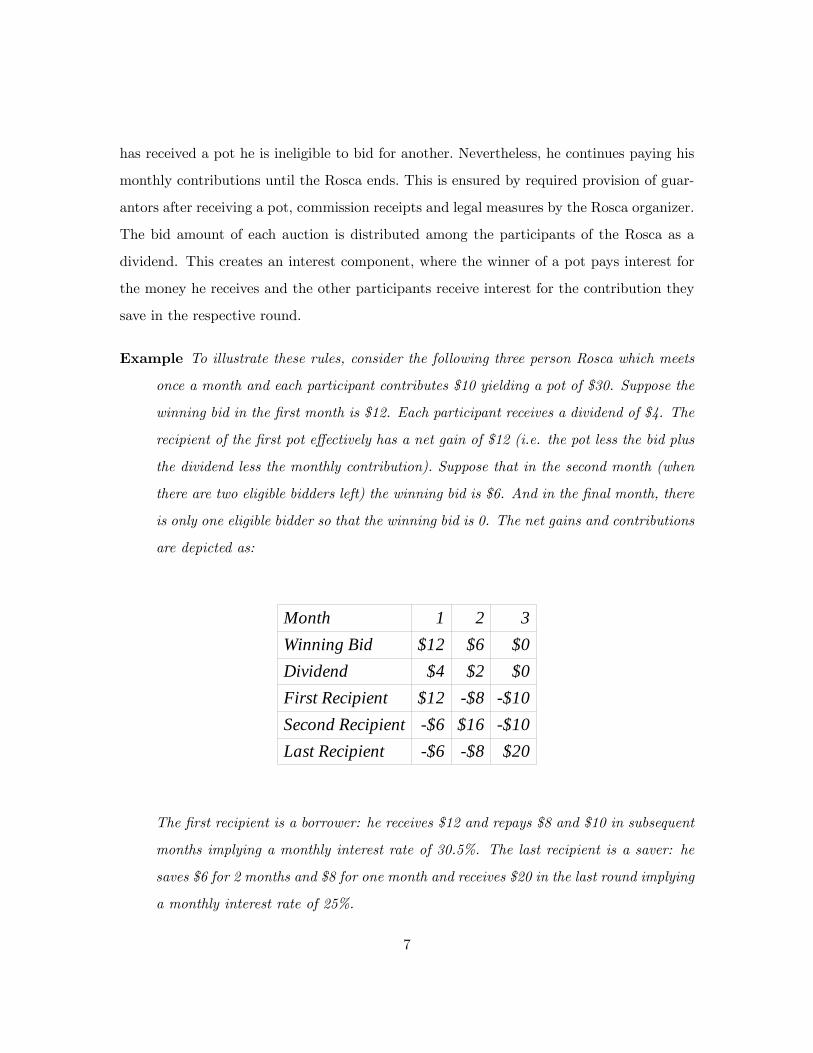
Example To illustrate these rules, consider the following three person Rosca which meets

once a month and each participant contributes $10 yielding a pot of $30. Suppose the

winning bid in the �rst month is $12. Each participant receives a dividend of $4. The

recipient of the �rst pot e¤ectively has a net gain of $12 (i.e. the pot less the bid plus

the dividend less the monthly contribution). Suppose that in the second month (when

there are two eligible bidders left) the winning bid is $6. And in the �nal month, there

is only one eligible bidder so that the winning bid is 0. The net gains and contributions

are depicted as:

Month 1 2 3Winning Bid $12 $6 $0Dividend $4 $2 $0First Recipient $12 $8 $10Second Recipient $6 $16 $10Last Recipient $6 $8 $20

The �rst recipient is a borrower: he receives $12 and repays $8 and $10 in subsequent

months implying a monthly interest rate of 30.5%. The last recipient is a saver: he

saves $6 for 2 months and $8 for one month and receives $20 in the last round implying

a monthly interest rate of 25%.

7

Due to the bidding process participants pay a di¤erent bid amount to get the pot and

hence a di¤erent interest rate, depending on their willingness to pay during the auction. We

exploit this variation in the bid amount in our empirical analysis.

The data set includes information on over 16,000 auctions from January 2004 to October

2005 of Rosca groups that started before December 2004. Each Rosca is uniquely identi�ed

by a group code and a branch code. The auctions within a Rosca are uniquely identi�ed by

the round of the Rosca. Generally, a Rosca facilitates borrowing and saving. As shown in

the example, the recipient of the �rst pot is a pure borrower and the recipient of the last pot

is a pure saver. For all auctions in between, the participation in the Rosca contains both

saving and credit components. The credit component dominates in earlier rounds whereas

the saving component dominates in later rounds.

The primary variable of interest in the present study is the bid amount as it proxies the

interest component. The pattern of the bid amount di¤ers across rounds. Generally, �rst

rounds of each Rosca produce the highest bid amounts. Early pot winners use the Rosca

to obtain funds that they repay by monthly subsequent contributions. Hence, they have a

high willingness to pay displayed in high bid amounts. Late pot winners use the Rosca as

a savings device. Hence, they want to receive the pot as late as possible to pay minimal

bid amounts. Those e¤ects lead to higher winning bids in earlier Rosca rounds and lower

winning bids in later rounds. Consequently, bid amounts decrease over the course of the

Rosca.

The data we use is from an established Rosca organizer with headquarters in Chennai.

This company started its business in Chennai, the state capital located in the Northeast

of Tamil Nadu in 1973 and has been expanding gradually since then. The Rosca organizer

o¤ers Roscas of di¤erent durations and monthly contributions resulting in various values of

the pot. This chit value ranges from 10,000 to 1,000,000 Indian Rupees with an average of

around 60,000 Indian Rupees (Table 1). The average winning bid in the sample is 13,131

Indian Rupees with a minimum of 500 Indian Rupees and a maximum of 300,000 Indian

8

Rupees.3 The relative bid amount de�ned as the winning bid relative to the respective chit

value allows comparison of bids across di¤erent denominations. It ranges from 5% to 40%

of the chit value with a sample mean of 19.75%. Rosca participants winning the auction

have to provide guarantors to secure continued contribution and repayment of the received

fund. The number of the so called cosigners ranges from zero to nine with an average of

1.57. Di¤erent participants use Roscas as a savings or borrowing device. On the one hand,

private individuals, participate in Roscas. On the other hand, �nancial institutions such

as banks participate in Roscas as institutional investors. The fraction of auctions won by

institutional investors in the sample is 38%. Rosca funds provided by this organizer are

used for productive investments and consumption alike (Klonner & Rai (2006); Klonner

(2008)).

3 Identi�cation Strategy and Estimation

For the analysis of the e¤ects of the Tsunami on credit demand we study the relative bid

amount in di¤erent Rosca groups. First, we divide all auction observations in the sample

into auctions taking place before the Tsunami and auctions taking place after the Tsunami

on December 26th in 2004. Second, we divide all branches into Tsunami a¤ected and

una¤ected branches. Overall, we look at 14 branches in the coastal area of Tamil Nadu

within a distance of 25 km from the coastline. Five branches are identi�ed as Tsunami

a¤ected branches and nine branches are identi�ed as una¤ected branches.4 All branches

within a proximity of 5 km to the coastline are classi�ed as a¤ected branches. This de�nition

3A commission of Rs. 500 has to be paid to the chairman of the Rosca at every auction. This poses the

bottom line of the winning bid amount. We only consider auctions in which a bidding took place indicated

by a winning bid amount higher than the commission. Further, the Indian government imposed a bid ceiling

on the winning bid amount of 40% of the chit value. With a maximum chit value of Rs. 1,000,000 the

maximum winning bid corresponds to Rs. 400,000.4A¤ected branches are the branches in Cuddalore, Karaikal, Nagappattinam, Pondicherry, and Tuticorin.

Una¤ected branches are branches in Chidambaram, Mayiladuthurai, Nagercoil, Pattukkottai, Ramanatha-

puram, Ramnad, Sirkazhi, Thiruthuraipondi, and Tiruvarur.

9

avoids any selection issues as the classi�cation solely depends on the branch�s distance to

the coastline. All branches within a distance of 5 to 25 km from the coastline are classi�ed

as una¤ected branches. The distances are measured with available geo information on

branch locations, coastlines and Tsunami survey points. Third, we combine the geophysical

information with the �nancial data. Every Rosca branch is assigned the run up height,

wave intensity and damage intensity measured at its closest Tsunami survey point.

We are interested in the e¤ect of the Tsunami on credit demand across branches. If

borrowing serves as a coping mechanism to aggregate shocks, we expect a higher demand

for borrowing in a¤ected branches driving up the winning bid in a Rosca. All Rosca groups

we are considering in the analysis started before the Tsunami, hence we are looking at

the e¤ect of the Tsunami on credit demand conditioned on participation in a Rosca. If

Roscas were used to mitigate the aggregate shock of the Tsunami hit, this is re�ected in an

increased relative bid amount after the Tsunami.

To estimate the increase in credit demand due to the Tsunami we compare the relative

winning bids in Tsunami a¤ected and una¤ected branches before and after the Tsunami. A

simple comparison of means in a¤ected and una¤ected branches already leads �rst indica-

tions. Before the Tsunami, the average relative bid amount in a¤ected branches is 21,8%.

It decreases to 17.07% after the Tsunami (Table 2). In una¤ected branches, the average

relative bid amount is 22% before the Tsunami and 15.57% after the Tsunami. Although

there is a general decrease over time, the decrease is stronger for una¤ected branches (-6.43

percentage points) than for a¤ected branches (-4.73 percentage points).

By applying di¤erence-in-di¤erence estimation technique we will estimate in equation

(1) whether the lower decrease in a¤ected branches is systematic and can be assigned to

the event of the Tsunami.

relative_bid_amountbgdr = � afterbgdr+� � affectedb + � � affectedb � afterbgdr

+xdr+ugdr (1)

The dependent variable is the relative_bid_amountbgdr which is the winning bid in

10

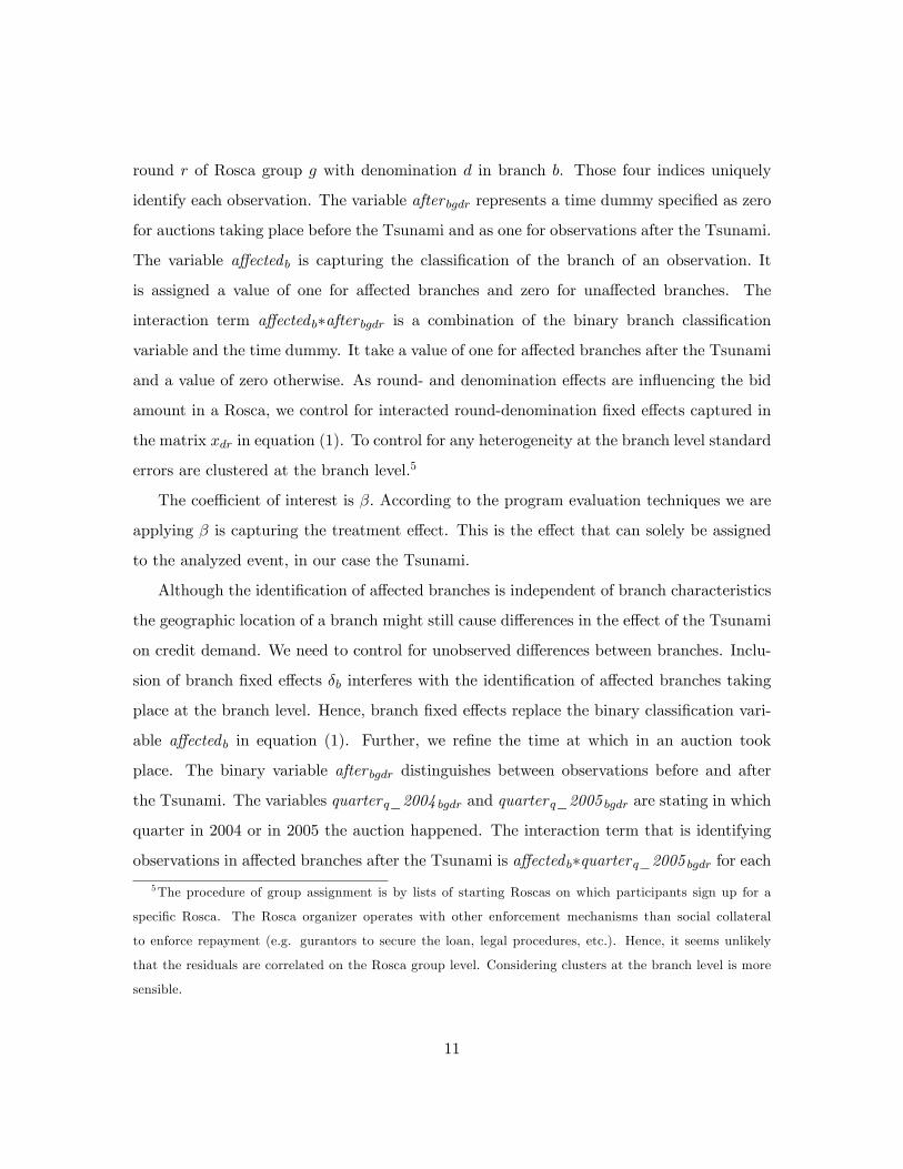
round r of Rosca group g with denomination d in branch b. Those four indices uniquely

identify each observation. The variable after bgdr represents a time dummy speci�ed as zero

for auctions taking place before the Tsunami and as one for observations after the Tsunami.

The variable a¤ected b is capturing the classi�cation of the branch of an observation. It

is assigned a value of one for a¤ected branches and zero for una¤ected branches. The

interaction term a¤ected b�after bgdr is a combination of the binary branch classi�cation

variable and the time dummy. It take a value of one for a¤ected branches after the Tsunami

and a value of zero otherwise. As round- and denomination e¤ects are in�uencing the bid

amount in a Rosca, we control for interacted round-denomination �xed e¤ects captured in

the matrix xdr in equation (1). To control for any heterogeneity at the branch level standard

errors are clustered at the branch level.5

The coe¢ cient of interest is �: According to the program evaluation techniques we are

applying � is capturing the treatment e¤ect. This is the e¤ect that can solely be assigned

to the analyzed event, in our case the Tsunami.

Although the identi�cation of a¤ected branches is independent of branch characteristics

the geographic location of a branch might still cause di¤erences in the e¤ect of the Tsunami

on credit demand. We need to control for unobserved di¤erences between branches. Inclu-

sion of branch �xed e¤ects �b interferes with the identi�cation of a¤ected branches taking

place at the branch level. Hence, branch �xed e¤ects replace the binary classi�cation vari-

able a¤ected b in equation (1). Further, we re�ne the time at which in an auction took

place. The binary variable after bgdr distinguishes between observations before and after

the Tsunami. The variables quarter q_2004 bgdr and quarter q_2005 bgdr are stating in which

quarter in 2004 or in 2005 the auction happened. The interaction term that is identifying

observations in a¤ected branches after the Tsunami is a¤ected b�quarter q_2005 bgdr for each5The procedure of group assignment is by lists of starting Roscas on which participants sign up for a

speci�c Rosca. The Rosca organizer operates with other enforcement mechanisms than social collateral

to enforce repayment (e.g. gurantors to secure the loan, legal procedures, etc.). Hence, it seems unlikely

that the residuals are correlated on the Rosca group level. Considering clusters at the branch level is more

sensible.

11

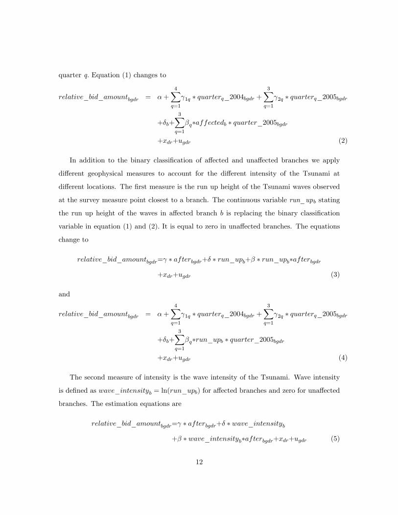
quarter q. Equation (1) changes to

relative_bid_amountbgdr = �+

4Xq=1

1q � quarterq_2004bgdr +3Xq=1

2q � quarterq_2005bgdr

+�b+3Xq=1

�q�affectedb � quarter_2005bgdr

+xdr+ugdr (2)

In addition to the binary classi�cation of a¤ected and una¤ected branches we apply

di¤erent geophysical measures to account for the di¤erent intensity of the Tsunami at

di¤erent locations. The �rst measure is the run up height of the Tsunami waves observed

at the survey measure point closest to a branch. The continuous variable run_upb stating

the run up height of the waves in a¤ected branch b is replacing the binary classi�cation

variable in equation (1) and (2). It is equal to zero in una¤ected branches. The equations

change to

relative_bid_amountbgdr= � afterbgdr+� � run_upb+� � run_upb�afterbgdr

+xdr+ugdr (3)

and


4Xq=1



+�b+

3Xq=1

�q�run_upb � quarter_2005bgdr

+xdr+ugdr (4)

The second measure of intensity is the wave intensity of the Tsunami. Wave intensity

is de�ned as wave_intensityb = ln(run_upb) for a¤ected branches and zero for una¤ected

branches. The estimation equations are

relative_bid_amountbgdr= � afterbgdr+� � wave_intensityb

+� � wave_intensityb�afterbgdr+xdr+ugdr (5)

12

and


4Xq=1



+�b+

3Xq=1

�q�wave_intensityb � quarter_2005bgdr

+xdr+ugdr (6)

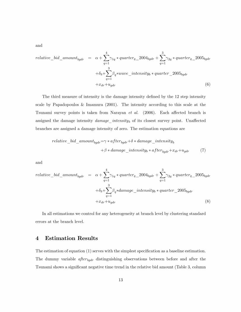
The third measure of intensity is the damage intensity de�ned by the 12 step intensity

scale by Papadopoulos & Imamura (2001). The intensity according to this scale at the

Tsunami survey points is taken from Narayan et al. (2006). Each a¤ected branch is

assigned the damage intensity damage_intensityb of its closest survey point. Una¤ected

branches are assigned a damage intensity of zero. The estimation equations are

relative_bid_amountbgdr= � afterbgdr+� � damage_intensityb

+� � damage_intensityb � afterbgdr+xdr+ugdr (7)

and

relative_bid_amountbgdr = �+4Xq=1



+�b+3Xq=1

�q�damage_intensityb � quarter_2005bgdr

+xdr+ugdr (8)

In all estimations we control for any heterogeneity at branch level by clustering standard

errors at the branch level.

4 Estimation Results

The estimation of equation (1) serves with the simplest speci�cation as a baseline estimation.

The dummy variable after bgdr distinguishing observations between before and after the

Tsunami shows a signi�cant negative time trend in the relative bid amount (Table 3, column

13

(1)). The interaction term a¤ected b�after bgdr identi�es the e¤ect on the relative bid amount

in a¤ected branches after the Tsunami. We observe a positive and signi�cant point estimate

of 0.815 percentage points corresponding to an increase in the relative bid amount of around

4% evaluated at the sample mean of the relative bid amount of 19.75%. The percent

increase corresponds to an increase in the interest rate implying that the interest rate is

higher in a¤ected branches after the Tsunami compared to the interest rate in una¤ected

areas. Re�ning the estimation equation by including branch �xed e¤ects and quarterly

time e¤ects (equation (2)) supports the �ndings of the baseline analysis qualitatively. We

observe a signi�cant increase of 1.05 percentage points in the relative bid amount in a¤ected

branches in the �rst quarter after the Tsunami (Table 3, column (2)). Evaluated at the

sample mean of the relative bid amount this corresponds to a rise of 5.3% of the interest

rate. The repercussion of the Tsunami in the �rst quarter is signi�cant at the 1% level

but its magnitude is limited. Further, we notice that this e¤ect fades away in the second

and third quarter after the Tsunami. From the signi�cant increase in the interest rate, we

conclude that credit demand actually intensi�ed in a¤ected branches in the �rst quarter

after the Tsunami. This pattern supports the idea that borrowing was used to bridge the

time lag until emergency relief and aid �ows started.

Exploiting the fact that Tsunami impact di¤ered along the coastline, we replace the

binary classi�cation in a¤ected and una¤ected branches by three di¤erent measures for the

Tsunami intensity. The �rst measure is the height of the Tsunami waves. Equation (3)

estimates the e¤ects of the run up height on the relative bid amount in a¤ected branches.

The coe¢ cient of the interaction term run_upb�after bgdr shows the e¤ect of the wave height

on the interest rate in a¤ected branches after the Tsunami. The signi�cant point estimate

of 0.136 con�rms that the relative bid amount is increasing in wave height (Table 3, column

(3)). Per one percent increase in wave height the relative bid amount increased by 0.68%

in a¤ected branches. Equation (4) disentangles the e¤ect over time. After the Tsunami, we

observe a point estimate of 0.132 at the 1% signi�cance level in the �rst quarter, a point

estimate of 0.180 at the 5% signi�cance level in the second quarter, and a point estimate

14

of 0.103 at the 10% signi�cance level in the third quarter in a¤ected branches (Table 3,

column (4)). Per one percent increase in wave height the relative bid amount increases by

0.5 to 0.9% in a¤ected branches in the three quarters after the Tsunami.

The second measure is the wave intensity as the logarithmic run up height. The inter-

action term wave_intensityb�after bgdr is measuring the e¤ect of the wave intensity on the

interest rate in a¤ected branches. In the simple speci�cation of equation (5) we observe a

signi�cant point estimate of 0.524 percentage points (Table 3, column (5)). This implies

an increase of 2.65% in the interest rate per additional meter in wave height evaluated at

an average borrowing rate of around 20%. The more re�ned speci�cation of equation (6)

with branch �xed e¤ects and quarterly time e¤ects shows that in the �rst quarter after the

Tsunami the relative bid amount increased by 0.575 percentage points at the 1% signi�-

cance level (Table 3, column (6)). In the second and third quarter there is an increase of

0.651 percentage points and 0.406 percentage points at the 10% signi�cance level. Those

estimates correspond to an increase in the interest rate of 2 to 3.3% per additional meter

of wave height.

The third measure of Tsunami intensity is the damage intensity based on observed dam-

age caused by the disaster. The estimation of equation (7) considers only a di¤erentiation

between observations before and after the shock. The interaction term damage_intensityb

�after bgdr has a signi�cant estimated coe¢ cient of 0.108. Per percent increase in the dam-

age intensity on the 12 step scale, the relative bid amount is increasing by 0.l08 percent

corresponding to a 0.5% increase evaluated at the sample borrowing rate of around 20 %

(Table 3, column (7)). After the Tsunami we observe a point estimate of 0.126 at the 1%

signi�cance level in the �rst quarter, a point estimate of 0.130 at the 10% signi�cance level

in the second quarter, and a point estimate of 0.0861 at the 10% signi�cance level in the

third quarter in a¤ected branches (Table 3, column (8)). Per one percent increase in the

damage intensity, the interest rate is increasing by 0.4 to 0.66% in the three quarters after

the Tsunami.

In our data we observe an increase in the interest rate in a¤ected branches after the

15

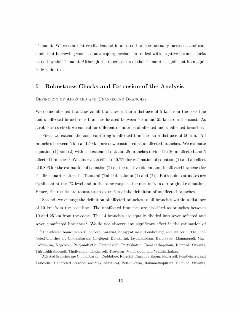
Tsunami. We reason that credit demand in a¤ected branches actually increased and con-

clude that borrowing was used as a coping mechanism to deal with negative income shocks

caused by the Tsunami. Although the repercussion of the Tsunami is signi�cant its magni-

tude is limited.

5 Robustness Checks and Extension of the Analysis

Definition of Affected and Unaffected Branches

We de�ne a¤ected branches as all branches within a distance of 5 km from the coastline

and una¤ected branches as branches located between 5 km and 25 km from the coast. As

a robustness check we control for di¤erent de�nitions of a¤ected and una¤ected branches.

First, we extend the zone capturing una¤ected branches to a distance of 50 km. All

branches between 5 km and 50 km are now considered as una¤ected branches. We estimate

equation (1) and (2) with the extended data on 25 branches divided in 20 una¤ected and 5

a¤ected branches.6 We observe an e¤ect of 0.750 for estimation of equation (1) and an e¤ect

of 0.896 for the estimation of equation (2) on the relative bid amount in a¤ected branches for

the �rst quarter after the Tsunami (Table 4, column (1) and (2)). Both point estimates are

signi�cant at the 1% level and in the same range as the results from our original estimation.

Hence, the results are robust to an extension of the de�nition of una¤ected branches.

Second, we enlarge the de�nition of a¤ected branches to all branches within a distance

of 10 km from the coastline. The una¤ected branches are classi�ed as branches between

10 and 25 km from the coast. The 14 branches are equally divided into seven a¤ected and

seven una¤ected branches.7 We do not observe any signi�cant e¤ect in the estimation of

6The a¤ected branches are Cuddalore, Karaikal, Nagappattinam, Pondicherry, and Tuticorin. The unaf-

fected branches are Chidambaram, Chigleput, Devakottai, Jayamkondam, Karaikkudi, Mannargudi, May-

iladuthurai, Nagercoil, Palayamkottai, Paramakudi, Pattukkottai, Ramanathapuram, Ramnad, Sirkazhi,

Thirutuhiraipoondi, Tindivanam, Tirunelveli, Tiruvarur, Villuparam, and Vriddhachalam.7A¤ected branches are Chidambaram, Cuddalore, Karaikal, Nagappattinam, Nagercoil, Pondicherry, and

Tuticorin. Una¤ected branches are Mayiladuthurai, Pattukkottai, Ramanathapuram, Ramnad, Sirkazhi,

16

equation (1) and only a marginally signi�cant positive point estimate for the �rst quarter

after the Tsunami in the estimation of equation (2) (Table 4, column (3) and (4)). Though

the sign of the estimated coe¢ cients is correct, they are mostly not signi�cant. We conclude

that the e¤ects of the Tsunami were limited to the area very close to the coastline.

Third, we maintain the extended de�nition of a¤ected branches at a 10 km distance and

additionally extend the de�nition of una¤ected branches to a distance between 10 and 50

km. The 25 branches are split up in seven a¤ected and 18 una¤ected branches.8 None of

the point estimates measuring the impact of the Tsunami in a¤ected branches is signi�cant.

Again we ascribe this to the geographical limitation of the Tsunami impact to locations

close to the coastline.

Placebo Experiment

We have to exclude the possibility that the results are driven by time trends unrelated

to the Tsunami and estimation problems with di¤erence-in-di¤erence estimation technique

in the presence of serial correlation.9 We conduct a placebo experiment with the same

speci�cations as in the estimation of the quasi-natural experiment by the Tsunami but

use a di¤erent time period. Instead of a balanced sample with observations of one year

before and one year after the Tsunami we shift back the considered time period for one year

and use data on observations from 2003 to 2004. The de�nition of a¤ected and una¤ected

branches stays the same as in the original analysis namely all branches closer than 5 km to

the coastline are classi�ed as a¤ected. We create an arti�cial event of a "Pseudo-Tsunami"

to happen at 26th December 2003 solely by de�nition of the time dummy after bgdr that

Thiruthuraipondi, and Tiruvarur.8A¤ected branches are Chidambaram, Cuddalore, Karaikal, Nagappattinam, Nagercoil, Pondicherry, and

Tuticorin. Una¤ected branches are Chidambaram, Chigleput, Devakottai, Jayamkondam, Karaikkudi, Man-

nargudi, Mayiladuthurai, Nagercoil, Palayamkottai, Paramakudi, Pattukkottai, Ramanathapuram, Ramnad,

Sirkazhi, Thirutuhiraipoondi, Tindivanam, Tirunelveli, Tiruvarur, Villuparam, and Vriddhachalam.9See Bertrand et al. (2004) for caveats of di¤erence-in-di¤erence estimation technique in the presence of

serial correlation.

17

divides the sample in observations before and after the shock. This date is exactly one

year before the real Indian Ocean Tsunami happened. All observations from 1st January

2003 to 26th December 2003 are classi�ed as "before Pseudo-Tsunami" and all observations

from 27th December 2003 to 31st December 2004 classi�ed as "after Pseudo-Tsunami". We

apply the same estimation techniques to the data set containing the pseudo event. Since

the "Pseudo-Tsunami" is marking an arti�cial event that did not actually take place we

expect to see no e¤ect in the data.

The data set we are using in the placebo experiment contains observations on 18,898

auctions from January 2003 to December 2004 (Table 5). It di¤ers from the originally

data set. The chit value ranges from 10,000 to 1,000,000 Indian Rupees with an average of

around 57,000 Indian Rupees (Table 5). The average winning bid in the sample is 15,618

Indian Rupees with a minimum of 500 Indian Rupees and a maximum of 400,000 Indian

Rupees.10 The relative bid amount as the winning bid relative to the respective chit value

allows comparison of bids across di¤erent denominations. It ranges from 5% to 40% of

the chit value with a sample mean of 24,42%. The number of cosigners required to secure

continued contribution and repayment of the received fund ranges from zero to ten with an

average of 1.87. The fraction of auctions won by other �nancial institutions taking part in

the Roscas as institutional investors is 37% in the sample.

The geophysical data used in the placebo experiment is the same as in the original

analysis. Due to a di¤erent partition of observations in a¤ected and una¤ected branches

the sample means di¤er slightly from the 2004-2005 data set. The run up height ranges from

3 to 11 meters averaging 5.69 meters in a¤ected areas considered in our study (Table 5). The

sample mean of the run up height corresponds to 2.58 meters. The �rst intensity measure

is the wave intensity. Average wave intensity is 1.63 in a¤ected branches and 0.74 in the

whole sample. The second measure is the damage intensity formed according to the 12 step

10A commission of Rs. 500 has to be paid to the chairman of the Rosca at every auction. This poses

the bottom line of the winning bid amount. Further, the Indian government imposed a bid ceiling on the

winning bid amount of 40% of the chit value. With a maximum chit value of Rs. 1,000,000 the maximum

winning bid corresponds to Rs. 400,000.

18

intensity scale by Papadopoulos & Imamura (2001) based on observable destruction caused

by a Tsunami. In a¤ected branches the damage intensity ranges from 6.5 corresponding

to the category "damaging" to a damage intensity of 10 corresponding to the category

"very destructive" on the 12 step intensity scale. The average damage intensity in a¤ected

branches is nearly 8 representing the category "heavy damaging". The sample mean of the

damage intensity is 3.6.

Estimation of equation (1) applying the placebo data yields an insigni�cant point esti-

mate of the impact on the "Pseudo-Tsunami" on the relative bid amount in a¤ected branches

compared to una¤ected branches. Also the re�ned estimation of equation (2) does not yield

any signi�cant estimates of an impact in any quarter after the "Pseudo-Tsunami" (Table

6, column (1) and (2)). Beyond the insigni�cance of the estimates, they all have the wrong

sign to show any positive impact. The same holds true for the analysis of the three Tsunami

intensity measures. Neither the run up height, nor the wave intensity or the damage inten-

sity show any signi�cant impact of the "Pseudo-Tsunami" in the a¤ected branches (Table

6, column (3)-(8)). We conclude that there can be no e¤ect on the "Pseudo-Tsunami" iden-

ti�ed on the relative bid amount that di¤ers for a¤ected and una¤ected branches. This is

naturally as expected since there was no real event taking place. Nevertheless it gives sub-

stantial con�dence that the results obtained in the impact evaluation of the real Tsunami

hit are not driven by any methodological e¤ects or the general negative time trend in the

data.

Structure of the Borrower Pool

There are other aspects which might be driving the results in the impact evaluation. After

su¤ering from material loss in the Tsunami a¤ected branches individuals are less desirable

borrowers for the Rosca organizer. To minimize default risk the Rosca organizer could be

trying to change the structure of the borrower pool of auction winners. Private persons

and �nancial institutions alike participate in Roscas to invest or obtain funds. Institutional

investors such as banks or semi-formal �nancial companies generally have a lower risk and

19

higher �nancial power. This allows them to pay higher interest rates and hence crowed

out private investors in an auction. Additionally, they are less likely to be a¤ected from

Tsunami destruction. Hence, they seem to be more desirable borrowers after the aggregate

shock. Consequently, the Rosca organizer could be trying to substitute private investors for

institutional ones.

If discouragement of private investors and encouragement of institutional investors as

a mean to reduce default risk after the Tsunami is fostered by the Rosca organizer, it

will most likely take informal forms. Hence, it is not observed in the data. However,

we can observe whether an institutional or a private investor is winning the auction. By

forming a binary variable institutional_investor bgdr that equals zero for private investors

and one for institutional investors we can analyze the linear probability of an institutional

investor receiving the funds. By applying di¤erence-in-di¤erence technique we test whether

institutional investors are more likely to receive the Rosca funds in a¤ected branches than in

una¤ected branches after the Tsunami. We estimate equations (1) to (8) but use the binary

variable for an institutional investor as the dependent variable. For instance, equation (1)

and (2) change to

institutional_investorbgdr= � afterbgdr+� � affectedb

+� � affectedb � afterbgdr+xdr+ugdr (1b)

and

institutional_investorbgdr=�+4Xq=1



+�b+3Xq=1

�q�affectedb � quarter_2005bgdr

+xdr+ugdr (2b)

The analysis using a binary classi�cation of a¤ected and una¤ected branches shows no

signi�cant impact of the Tsunami in a¤ected branches on the probability that an institu-

tional investor is receiving the Rosca funds (Table 7, column (1) and (2)). The same holds

20

true for the three measures of Tsunami intensity, namely the run up height, the wave inten-

sity and the damage intensity (Table 7, column (3) to (8)). We conclude that the observed

increase in the interest rate is not driven by a change in the structure of the borrower pool

from private to institutional investors.

Other loan characteristics

A way to discourage borrowers from obtaining funds is increasing indirect costs of credit.

Generally, upon receiving a pot, borrowers have to provide guarantors, so called cosigners,

to secure repayment and continued contributions to the Rosca. The number of cosigners

or guarantors required to pledge the reception of the chit value is one measure of such

indirect costs. By demanding more cosigners the semi-formal institution studied here can

augment such indirect costs and discourage a¤ected individuals from obtaining funds. By

applying di¤erence-in-di¤erence technique we test whether the number of required cosigners

has increased after the Tsunami in a¤ected areas. We estimate equations (1) to (8) but use

the number of cosigners as the dependent variable cosignersbgdr. For instance, equation (1)

and (2) change to

cosignersbgdr = � afterbgdr+� � affectedb

+� � affectedb � afterbgdr+xdr+ugdr (1c)

and

cosignersbgdr = �+4Xq=1



+�b+3Xq=1

�q�affectedb � quarter_2005bgdr + xdr+ugdr (2c)

The analysis using a binary classi�cation of a¤ected and una¤ected branches shows no

signi�cant impact of the Tsunami in a¤ected branches on the number of cosigners (Table 8,

column (1) and (2)). The same holds true for the three measures of Tsunami intensity, the

run up height, the wave intensity and the damage intensity, respectively (Table 8, column

21

(3) to (8)). We conclude that the observed increase in the interest rate is not driven by a

change in required securities to pledge the borrowed funds.

6 Conclusion

In this study, we use geophysical data and detailed �nancial data from a semi-formal �nan-

cial institution organizing Roscas in Tamil Nadu to investigate directly changes in credit

demand caused by the Indian Ocean Tsunami of 26 December, 2004. A di¤erence-in-

di¤erence approach is applied to test for changes in the interest rate in a¤ected branches

compared to the una¤ected branches after the Tsunami.

We �nd a positive and signi�cant increase in the relative bid amount in the a¤ected

branches after the Tsunami. This corresponds to a 5.3% increment in the interest rate in

the �rst quarter in 2005 that can be attributed to the Tsunami hit re�ecting an overall

expansion of credit demand in a¤ected branches. Accounting for the treatment intensity

measured by run up height and wave intensity we observe a raise in the interest rate in the

�rst quarter after the Tsunami of 0.6% per one percent increase in the wave height and an

increase of the interest rate of around 3% per additional meter of wave height.

We conclude that local funds provided by Roscas did play a role in coping with the after-

e¤ects of the Tsunami. Although Roscas only pool local resources, they seem to provide

insurance against aggregate shocks. Nevertheless, the deployment of Rosca funds is limited

in terms of the magnitude of e¤ects. The signi�cant positive e¤ect in the �rst three months

after the Tsunami hit subsequently diminished in later months. This latter observation is

in line with qualitative evidence on aid �ows and relief programs which are reported to

have reached the a¤ected areas with a time lag of several months. In this connection, our

results suggest that semi-formal credit and o¢ cial aid are substitutes as disaster coping

mechanisms, rather than complements.

22

References

AsianDevelopmentBank. 2005. An Initial Assessment of the Impact of the Earthquake

and Tsunami of December 26, 2004 on South and Southeast Asia.

Athukorala, Prema-Chandra, & Resosudarmo, Budy P. 2005. The Indian Ocean

Tsunami: Economic Impact, Disaster Management and Lessons. Asian Economic Papers,

4(1), 1�39.

Beegle, Kathleen, Dehejia, Rajeev, & Gatti, Roberta. 2006. Child Labor and

Agricultural Shocks. Journal of Development Economics, 81, 80�96.

Bertrand, Marianne, Duflo, Esther, & Mullainathan, Sendhil. 2004. How Much

Should We Trust Di¤erence-In-Di¤erence Estimates? Quarterly Journal of Economics,

119(1), 249�275.

Del Ninno, Carlo, Dorosh, Paul A., & Smith, Lisa C. 2003. Public Policy, Mar-

kets and Household Coping Strategies in Bangladesh: Avoiding a Food Security Crisis

Following the 1998 Floods. World Development, 31(7), 1221�1238.

Eswaran, Mukesh, & Kotwal, Ashok. 1989. Credit as Insurance in Agrarian

Economies. Journal of Development Economics, 31, 37�53.

Gertler, Paul, Levine, David I., & Moretti, Enrico. 2002. Do Micro�nance Pro-

grams Help Families Insure Consumption Against Illness? California Center for Popula-

tion Research On-line Working Paper Series.

Gitter, Seth R., & Barham, Bradford L. 2007. Credit, Natural Disasters, Co¤ee,

and Educational Attainment in Rural Honduras. World Development, 35(3), 498�511.

Guarcello, Lorenzo; Mealli, Fabrizia; Rosati Furio Camillo. 2009. Household

vulnerability and child labor: the e¤ect of shocks, credit rationing, and insurance. Journal

of Population Economics, 23(1), 169�198.

23

Jacoby, Hanan G., & Skoufias, Emmanuel. 1997. Risk, Financial Markets, and Human

Capital in a Developing Country. Review of Economic Studies, 64, 311�335.

Khandker, Shahidur R. 2007. Coping with Flood: Role of Institutions in Bangladesh.

Agricultural Economics, 36(2), 169 �180.

Klonner, Stefan. 2008. Private Information and Altruism in Bidding Roscas. The

Economic Journal, 118(528), 775�800.

Klonner, Stefan, & Rai, Ashok. 2006. Adverse Selection in Credit Marktes: Evidence

from Bidding Roscas. Working Paper, Cornell Universtiy, Williams College.

Maheshwari, B.K., Sharma, M.L., & Narayan, J.P. 2005. Structural Damages on the

Coast of Tamil Nadu Due to Tsunami Caused by December 26, 2004 Sumatra Earthquake.

ISET Journal of Earthquake Technology, 42(2-3), 63�78.

Narayan, J.P., Sharma, M.L., & Maheshwari, B.K. 2005. Run-Up and Inundation

Pattern Developed During the Ocean Tsunami of December 26, 2004 Along the Coast of

Tamilnadu (India). Gondwana Research, 8(4), 611�616.

Narayan, J.P., Sharma, M.L., & Maheshwari, B.K. 2006. Tsunami Intensity Mapping

Along the Coast of Tamilnadu (India) During the Deadliest Indian Ocean Tsunami of

December 26, 2004. Pure and Applied Geophysics, 163, 1279�1304.

Papadopoulos, A., & Imamura, Fumihiko. 2001. A Proposal for a New Tsunami

Intensity Scale. ITS Proceedings, 5(5-1), 569�577.

Sawada, Yasuyuki. 2008. How Do People Cope with Natural Disasters? Evidence from

the Great Hanshin-Awaji (Kobe) Earthquake in 1995. Journal of Money, Credit and

Banking, 40(2-3), 463�488.

Skoufias, Emmanuel. 2003. Economic Crises and Natural Disasters: Coping Strategies

and Policy Implications. World Development, 31(7), 1087 � 1102. Economic Crises,

Natural Disasters, and Poverty.

24

TamilNaduGovernment. 2005. Tsunami: Impact & Damage.

Townsend, Robert. 1994. Risk and Insurance in Village India. Econometrica, 62((2)),

539�591.

Udry, Christopher. 1990. Credit Markets in Northern Nigeria: Credit as Insurance in a

Rural Economy. World Bank Econ Rev, 4(3), 251�269.

Udry, Christopher. 1994. Risk and Insurance in a Rural Credit Market: An Empirical

Investigation in Northern Nigeria. Review of Economic Studies, 61, 495�526.

25

Figure 1: Tsunami Hit Locations, Rosca Branches and Tsunami Intensity in Tamil Nadu

Table 1

Mean Standard Deviation Minimum Maximum

All Branches (16,419 Observations)

Financial Data

Chit Value (INR) 60,200.99 102,338.30 10,000 1,000,000

Duration in Month 37.22 6.63 25 60

Monthly Contribution 1,608.75 2,642.03 200 30,000

Bid Amount (INR) 13,131.20 26,158.22 520 300,000

Relative Bid Amount 0.1975 0.1087 0.0504 0.4

Number of Cosigners* 1.5662 1.2403 0 9

Institutional Investor Dummy 0.3753 0.4842 0 1

Geophysical Data**

Run Up Height (meter) 2.5924 3.4390 0 11

Wave Intensity 0.7377 0.8749 0 2.3979

Damage Intensity 3.5683 4.0704 0 10

Unaffected Branches (9,077 Observations)

Financial Data

Chit Value (INR) 55,797.07 90,816.60 10,000 1,000,000



Bid Amount (INR) 12,171.96 24,055.83 520 240,000




Geophysical Data**

Run Up Height (meter) 0 0 0 0

Wave Intensity 0 0 0 0

Damage Intensity 0 0 0 0

Affected Branches (7,342 Observations)

Financial Data

Chit Value (INR) 65,645.60 114,770.90 10,000 1,000,000



Bid Amount (INR) 14,317.12 28,501.26 525 300,000

Relative Bid Amount 0.2003 0.1097 0 0



Geophysical Data**


Wave Intensity 1.6497 0.4552 1.0986 2.3979

Damage Intensity 7.9799 1.3588 6.5 10

Descriptive Statistics of Auctions in 2004‐2005

Calculations are based on data Rosca auctions from January 2004‐October 2005 in Tamil Nadu in branches within 25 km distance of coastline. Only auctions with a bid amount higher than the commission are considered to ensure a bidding process took place. Bid Amount: Winning bid amount of auction. Relative Bid Amount: bid amount as fraction of chit value. Institutional Investor Dummy: 1 if auction is won by an institutional investor, 0 otherwise. Run up height: Maximum height of water observed above a reference sea level (height in meter). Wave intensity=ln(run up height). Damage Intensity by 12 step intensity scale: I) Not felt, II) Scarcely felt, III) Weak, IV) Largely observed, V) Strong, VI) Slightly damaging, VII) Damaging, VIII) Heavy damaging, IX) Destructive, X) Very destructive, XI) Devastating, and XII) Completely Devastating. *only for groups that reported cosigner data (8,935 auctions, 4,904 in unaffected branches, 4,031 in affected branches).** based on tsunami survey measure points of the Indian Institute of Technology Roorkee, India for affected branches.

Table 2

Before Tsunami After Tsunami Difference Significance Level of Difference

All Branches 21.90 16.23 ‐5.67 p<1%(0.10922) (0.1222) (0.16904)

Affected Branches 21.80 17.07 ‐4.73 p<1%(0.16661) (0.18604) (0.25794)

Unaffected Branches 22.00 15.57 ‐6.43 p<1%(0.14446) (0.16103) (0.22313)

Dependent variable: relative bid amount. No fixed effects included. All entries times 100, since dependent variable is a fraction (bid amount/ chit value). Standard errors in parenthesis. Observations of auctions from January 2004‐October 2005. (1) All branches in Tamil Nadu within a distance of 25 km from coastline. (2) Only affected branches within a distance of 5km from coast line. (3) Unaffected branches within a distance of 5km to 25km from coast line.

Relative Bid Amount

Average Relative Bid Amount Before and After the Tsunami

Tsunami Measure:(1) (2) (3) (4) (5) (6) (7) (8)

Constant 9.20*** 37.7*** 7.47*** 31.4*** 7.15*** 31.7*** 9.23*** 37.6***(0.325) (0.416) (1.14) (0.608) (0.965) (0.565) (0.317) (0.403)

Tsunami Measure (Dummy) ‐8.21 ‐0.0635 ‐0.16 ‐0.0203(0.618) (0.104) (0.403) (0.0833)

After Tsunami (Dummy) ‐1.70*** ‐1.69*** ‐1.73*** ‐1.73***(0.325) (0.298) (0.310) (0.317)0.815** 0.136*** 0.524** 0.108**(0.351) (0.0418) (0.187) (0.0419)

1. Quarter 2004 (Dummy) 2.32*** 2.37*** 2.39*** 2.37***(0.416) (0.373) (0.394) (0.403)

2. Quarter 2004 (Dummy) 2.09*** 2.15*** 2.16*** 2.15***(0.538) (0.488) (0.511) (0.523)

3. Quarter 2004 (Dummy) 1.68*** 1.73*** 1.75*** 1.73***(0.446) (0.403) (0.424) (0.434)

4. Quarter 2004 (Dummy) 1.25*** 1.31*** 1.32*** 1.30***(0.334) (0.315) (0.340) (0.342)

1. Quarter 2005 (Dummy) 0.193 0.376 0.307 0.268(0.287) (0.271) (0.279) (0.282)

3. Quarter 2005 (Dummy) ‐0.315* ‐0.239 ‐0.259 ‐0.281*(0.154) (0.159) (0.162) (0.158)

Tsunami Measure x 1.Quarter 2005 1.05*** 0.132*** 0.575*** 0.126***(Dummy) (0.288) (0.0380) (0.160) (0.0349)Tsunami Measure x 2.Quarter 2005 0.922 0.180** 0.651* 0.130*(Dummy) (0.532) (0.0725) (0.314) (0.0676)Tsunami Measure x 3.Quarter 2005 0.644 0.103* 0.406* 0.0861*(Dummy) (0.403) (0.0509) (0.218) (0.0480)Observations 16419 16419 16419 16419 16419 16419 16419 16419R‐squared 0.797 0.804 0.797 0.804 0.797 0.804 0.797 0.804Round‐Denomination Fixed Effects Yes Yes Yes Yes Yes Yes Yes YesBranch Fixed Effects No Yes No Yes No Yes No Yes

Difference‐in‐Difference‐Estimation of the Relative Bid Amount in 2004 and 2005 on Different Tsunami Measures

Tsunami Measure x After Tsunami (Dummy)

All coefficients times 100, since they are representing fractions (relative bid amount). Observations from January 2004‐October 2005. Dependent Variable: Relative Bid Amount. Affected branches within 5 km distance from coast, unaffected branches within 5 ‐ 25km distance from coast.(1)‐(2) Binary classification in affected and unaffected branches, (3)‐(4) Run up height, (5)‐(6) wave intensity=ln(run up height), (7)‐(8) damage intensity by 12 step intensity scale by Papadopoulos and Imamura (2001). Round‐Denomination Fixed Effects included in all regressions. Branch Fixed Effects included as indicated. Standard errors clustered at branch level. Robust standard errors in parentheses. *** p<0.01, ** p<0.05, * p<0.1

Affected Branches Run Up Height Wave Intensity Damage Intensity

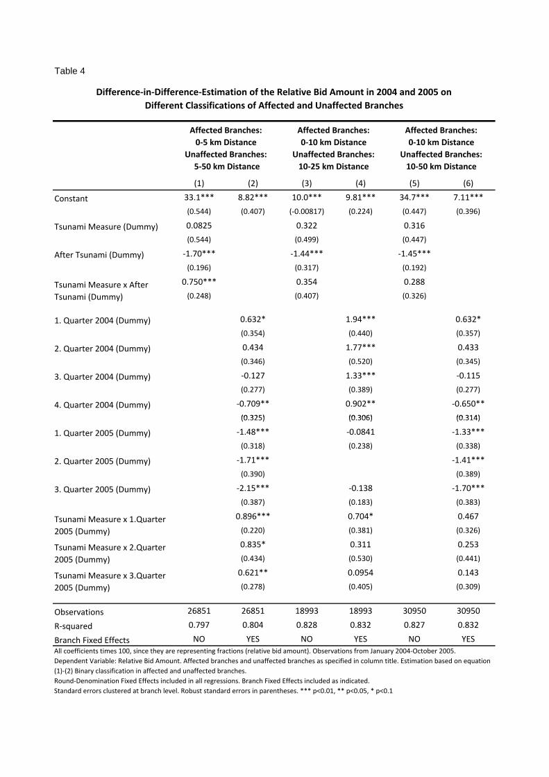
Table 4

(1) (2) (3) (4) (5) (6)

Constant 33.1*** 8.82*** 10.0*** 9.81*** 34.7*** 7.11***

(0.544) (0.407) (‐0.00817) (0.224) (0.447) (0.396)

Tsunami Measure (Dummy) 0.0825 0.322 0.316

(0.544) (0.499) (0.447)

After Tsunami (Dummy) ‐1.70*** ‐1.44*** ‐1.45***

(0.196) (0.317) (0.192)

0.750*** 0.354 0.288

(0.248) (0.407) (0.326)

1. Quarter 2004 (Dummy) 0.632* 1.94*** 0.632*

(0.354) (0.440) (0.357)

2. Quarter 2004 (Dummy) 0.434 1.77*** 0.433

(0.346) (0.520) (0.345)

3. Quarter 2004 (Dummy) ‐0.127 1.33*** ‐0.115

(0.277) (0.389) (0.277)

4. Quarter 2004 (Dummy) ‐0.709** 0.902** ‐0.650**

(0 325) (0 306) (0 314)

Difference‐in‐Difference‐Estimation of the Relative Bid Amount in 2004 and 2005 on Different Classifications of Affected and Unaffected Branches

Affected Branches:0‐5 km Distance

Unaffected Branches: 5‐50 km Distance

Affected Branches: 0‐10 km Distance


Affected Branches: 0‐10 km Distance



(0.325) (0.306) (0.314)

1. Quarter 2005 (Dummy) ‐1.48*** ‐0.0841 ‐1.33***

(0.318) (0.238) (0.338)

2. Quarter 2005 (Dummy) ‐1.71*** ‐1.41***

(0.390) (0.389)

3. Quarter 2005 (Dummy) ‐2.15*** ‐0.138 ‐1.70***

(0.387) (0.183) (0.383)

0.896*** 0.704* 0.467

(0.220) (0.381) (0.326)

0.835* 0.311 0.253

(0.434) (0.530) (0.441)

0.621** 0.0954 0.143

(0.278) (0.405) (0.309)

Observations 26851 26851 18993 18993 30950 30950

R‐squared 0.797 0.804 0.828 0.832 0.827 0.832

Branch Fixed Effects NO YES NO YES NO YESAll coefficients times 100, since they are representing fractions (relative bid amount). Observations from January 2004‐October 2005. Dependent Variable: Relative Bid Amount. Affected branches and unaffected branches as specified in column title. Estimation based on equation (1)‐(2) Binary classification in affected and unaffected branches. Round‐Denomination Fixed Effects included in all regressions. Branch Fixed Effects included as indicated. Standard errors clustered at branch level. Robust standard errors in parentheses. *** p<0.01, ** p<0.05, * p<0.1

Tsunami Measure x 3.Quarter 2005 (Dummy)



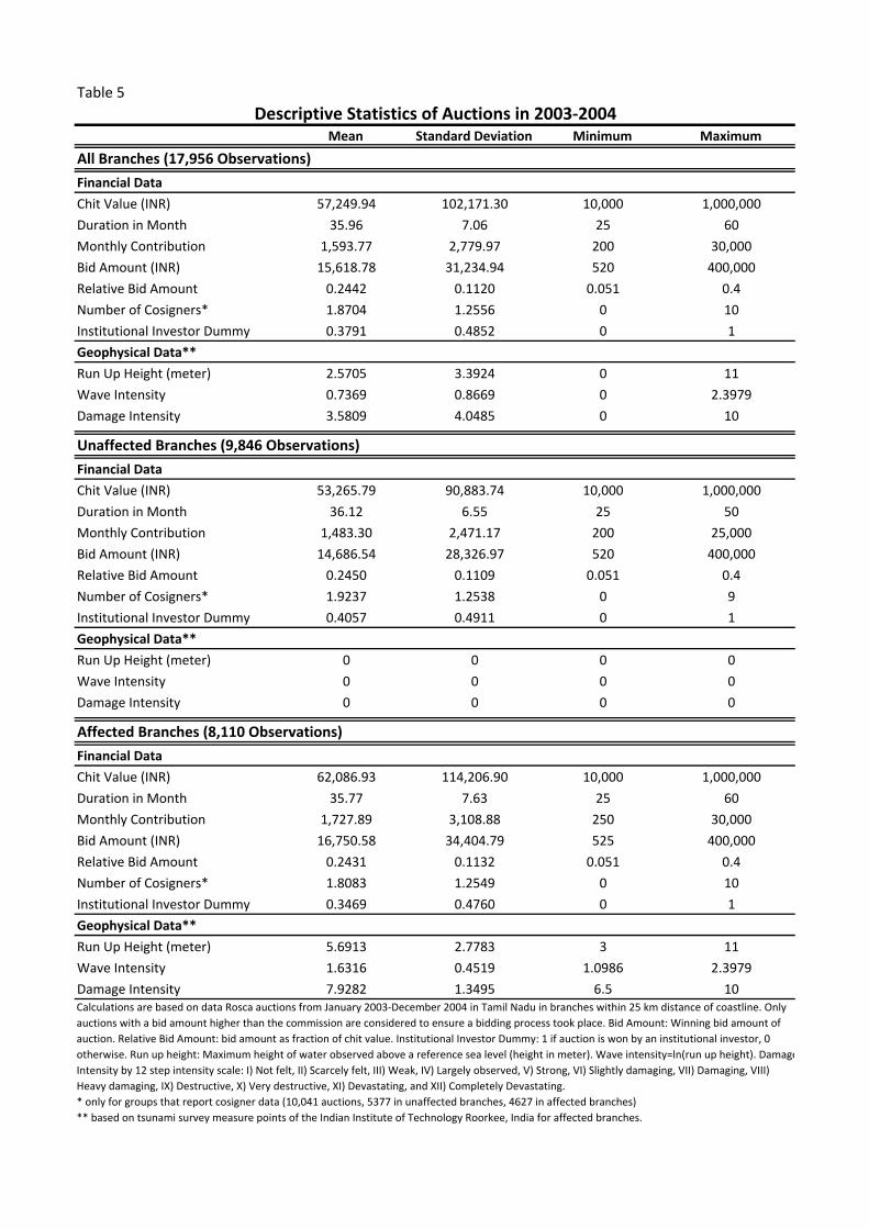
Table 5

Mean Standard Deviation Minimum Maximum

All Branches (17,956 Observations)

Financial Data

Chit Value (INR) 57,249.94 102,171.30 10,000 1,000,000



Bid Amount (INR) 15,618.78 31,234.94 520 400,000




Geophysical Data**


Wave Intensity 0.7369 0.8669 0 2.3979

Damage Intensity 3.5809 4.0485 0 10

Unaffected Branches (9,846 Observations)

Financial Data

Chit Value (INR) 53,265.79 90,883.74 10,000 1,000,000



Bid Amount (INR) 14,686.54 28,326.97 520 400,000




Geophysical Data**

Run Up Height (meter) 0 0 0 0

Wave Intensity 0 0 0 0

Damage Intensity 0 0 0 0

Affected Branches (8,110 Observations)

Financial Data

Chit Value (INR) 62,086.93 114,206.90 10,000 1,000,000



Bid Amount (INR) 16,750.58 34,404.79 525 400,000




Geophysical Data**


Wave Intensity 1.6316 0.4519 1.0986 2.3979

Damage Intensity 7.9282 1.3495 6.5 10

Descriptive Statistics of Auctions in 2003‐2004

Calculations are based on data Rosca auctions from January 2003‐December 2004 in Tamil Nadu in branches within 25 km distance of coastline. Only auctions with a bid amount higher than the commission are considered to ensure a bidding process took place. Bid Amount: Winning bid amount of auction. Relative Bid Amount: bid amount as fraction of chit value. Institutional Investor Dummy: 1 if auction is won by an institutional investor, 0 otherwise. Run up height: Maximum height of water observed above a reference sea level (height in meter). Wave intensity=ln(run up height). DamageIntensity by 12 step intensity scale: I) Not felt, II) Scarcely felt, III) Weak, IV) Largely observed, V) Strong, VI) Slightly damaging, VII) Damaging, VIII) Heavy damaging, IX) Destructive, X) Very destructive, XI) Devastating, and XII) Completely Devastating. * only for groups that report cosigner data (10,041 auctions, 5377 in unaffected branches, 4627 in affected branches) ** based on tsunami survey measure points of the Indian Institute of Technology Roorkee, India for affected branches.

Table 6

Tsunami Measure:(1) (2) (3) (4) (5) (6) (7) (8)

Constant 6.25*** 4.54*** 31.4*** 10.7*** 31.1*** 4.53*** 31.0*** 4.54***(0.687) (0.304) (1.17) (0.548) (0.996) (0.311) (0.875) (0.310)

Tsunami Measure (Dummy) 0.0975 0.00821 0.0465 0.0146(0.530) (0.0628) (0.280) (0.0625)

After Tsunami (Dummy) ‐0.959** ‐0.823** ‐0.872** ‐0.909**(0.354) (0.341) (0.355) (0.356)‐0.0499 ‐0.0623 ‐0.149 ‐0.0204(0.457) (0.0803) (0.312) (0.0635)

1. Quarter 2004 (Dummy) 1.54** 1.54** 1.54** 1.54**(0.548) (0.548) (0.548) (0.549)

2. Quarter 2004 (Dummy) 1.91*** 1.92*** 1.92*** 1.91***(0.485) (0.485) (0.485) (0.485)

3. Quarter 2004 (Dummy) 1.54*** 1.54*** 1.54*** 1.54***(0.493) (0.493) (0.493) (0.493)

4. Quarter 2004 (Dummy) 1.60** 1.60** 1.60** 1.60**(0.540) (0.540) (0.540) (0.540)

1. Quarter 2005 (Dummy) 1.11** 1.28*** 1.23** 1.19**(0.468) (0.413) (0.438) (0.450)

2. Quarter 2005 (Dummy) 1.05* 1.13** 1.12** 1.09**(0.486) (0.463) (0.480) (0.486)

3. Quarter 2005 (Dummy) 0.627* 0.620* 0.635* 0.631*(0.304) (0.319) (0.311) (0.310)

Tsunami Measure x 1.Quarter 2005 ‐0.271 ‐0.116* ‐0.339 ‐0.0574(Dummy) (0.435) (0.0600) (0.273) (0.0579)Tsunami Measure x 2.Quarter 2005 ‐0.581 ‐0.135 ‐0.449 ‐0.0842(Dummy) (0.518) (0.0803) (0.336) (0.0707)Tsunami Measure x 3.Quarter 2005 ‐0.389 ‐0.0652 ‐0.25 ‐0.0502(Dummy) (0.440) (0.0638) (0.259) (0.0553)Observations 17956 17956 17956 17956 17956 17956 17956 17956R‐squared 0.791 0.798 0.791 0.798 0.791 0.798 0.791 0.798Branch Fixed Effects NO YES NO YES NO YES NO YESPlacebo Experiment: Observations from January 2003‐October 2004. All coefficients times 100, since they are representing fractions (relative bid amount). Dependent Variable: Relative Bid Amount. Affected branches within 5 km distance from coast, unaffected branches within 5 ‐ 25km distance from coast.(1)‐(2) Binary classification in affected and unaffected branches, (3)‐(4) Run up heigth, (5)‐(6) wave intensity=ln(run up height), (7)‐(8) damage intensity by 12 step intensity scale by Papadopoulos and Imamura (2001). Round‐Denomination Fixed Effects included in all regressions. Branch Fixed Effects included as indicated. Standard errors clustered at branch level. Robust standard errors in parentheses. *** p<0.01, ** p<0.05, * p<0.1

Placebo Experiment: Estimation of the Relative Bid Amount in 2003 and 2004 on Different Tsunami Measures of "Pseudo‐Tsunami"Affected Branches Run Up Height Wave Intensity Damage Intensity


Table 7

Tsunami Measure:(1) (2) (3) (4) (5) (6) (7) (8)

Constant 0.0363 1.144*** 0.0309 ‐0.0205 0.0201 1.111*** 0.0421 1.080***(0.0347) (0.0147) (0.0619) (0.0276) (0.0520) (0.00742) (0.0462) (0.0162)

Tsunami Measure (Dummy) ‐0.0363 ‐0.00281 ‐0.0167 ‐0.00421(0.0347) (0.00563) (0.0221) (0.00462)

After Tsunami (Dummy) ‐0.00736 ‐0.0136 ‐0.0129 ‐0.0114(0.0163) (0.0148) (0.0157) (0.0159)0.00967 0.00418* 0.0137 0.00238(0.0227) (0.00221) (0.0104) (0.00250)

1. Quarter 2004 (Dummy) ‐0.0360 0.00392 ‐0.0285 0.000532(0.0240) (0.0289) (0.0224) (0.0291)

2. Quarter 2004 (Dummy) ‐0.0359* 0.00420 ‐0.0283 0.000683(0.0187) (0.0274) (0.0189) (0.0285)

3. Quarter 2004 (Dummy) ‐0.0123 0.0275 ‐0.00484 0.0242(0.0170) (0.0235) (0.0175) (0.0241)

4. Quarter 2004 (Dummy) 0.000568 0.0405* 0.00807 0.0371(0.0162) (0.0209) (0.0152) (0.0232)

1. Quarter 2005 (Dummy) ‐0.0329** ‐0.0315**(0 0140) (0 0128)

Difference‐in‐Difference‐Estimation of the Institutional Investor on Different Tsunami MeasuresAffected Branches Run Up Height Wave Intensity Damage Intensity


(0.0140) (0.0128)2. Quarter 2005 (Dummy) 0.0289** 0.0316**

(0.0126) (0.0133)3. Quarter 2005 (Dummy) ‐0.0218 0.0149 ‐0.0180 0.0115

(0.0175) (0.0174) (0.0169) (0.0184)Tsunami Measure x 1.Quarter 2005 0.0200 0.00622 0.0205 0.00353(Dummy) (0.0342) (0.00371) (0.0166) (0.00386)Tsunami Measure x 2.Quarter 2005 ‐0.0275 ‐0.000392 ‐0.00634 ‐0.00204(Dummy) (0.0234) (0.00249) (0.0123) (0.00287)Tsunami Measure x 3.Quarter 2005 0.0150 0.00381 0.0141 0.00278(Dummy) (0.0265) (0.00313) (0.0135) (0.00308)Observations 18993 18993 18993 18993 18993 18993 18993 18993R‐squared 0.284 0.307 0.284 0.307 0.284 0.307 0.284 0.307Branch Fixed Effects NO YES NO YES NO YES NO YES Observations from January 2004‐October 2005. Dependent Variable: Institutional Investor. Affected branches within 5 km distance from coast, unaffected branches within 5 ‐ 25km distance from coast.(1)‐(2) Binary classification in affected and unaffected branches, (3)‐(4) Run up heigth, (5)‐(6) wave intensity=ln(run up height), (7)‐(8) damage intensity by 12 step intensity scale by Papadopoulos and Imamura (2001). Round‐Denomination Fixed Effects included in all regressions. Branch Fixed Effects included as indicated. Standard errors clustered at branch level. Robust standard errors in parentheses. *** p<0.01, ** p<0.05, * p<0.1

Table 8

Tsunami Measure:(1) (2) (3) (4) (5) (6) (7) (8)

Constant 1.106*** 0.952*** 4.063*** ‐0.177* 4.089*** ‐0.115* 3.057*** ‐0.114*(0.0719) (0.0526) (0.116) (0.0846) (0.109) (0.0616) (0.133) (0.0610)

Tsunami Measure (Dummy) ‐0.0744 0.00388 ‐0.0104 ‐0.00571(0.0875) (0.0171) (0.0666) (0.0133)

After Tsunami (Dummy) ‐0.0128 0.00458 ‐0.00169 ‐0.00603(0.0336) (0.0310) (0.0332) (0.0338)‐0.0186 ‐0.00999 ‐0.0259 ‐0.00410(0.0461) (0.00912) (0.0347) (0.00682)

1. Quarter 2004 (Dummy) ‐0.0771 ‐0.0605 ‐0.0590 ‐0.0545(0.0630) (0.0702) (0.0721) (0.0735)

2. Quarter 2004 (Dummy) 0.00370 0.0207 0.0221 0.0265(0.0480) (0.0446) (0.0460) (0.0467)

3. Quarter 2004 (Dummy) ‐0.000321 0.0180 0.0189 0.0230(0.0397) (0.0472) (0.0511) (0.0520)

4. Quarter 2004 (Dummy) ‐0.0302 ‐0.0122 ‐0.0112 ‐0.00708(0.0437) (0.0533) (0.0578) (0.0592)

1. Quarter 2005 (Dummy) ‐0.0637 ‐0.0168 ‐0.0270 ‐0.0290(0.0372) (0.0319) (0.0315) (0.0319)

2. Quarter 2005 (Dummy) 0.0327 0.0337 0.0334(0.0382) (0.0399) (0.0401)

3. Quarter 2005 (Dummy) ‐0.0326(0.0394)

Tsunami Measure x 1.Quarter 2005 0.0174 ‐0.00893 ‐0.0147 ‐0.00119(Dummy) (0.0714) (0.0101) (0.0447) (0.00918)Tsunami Measure x 2.Quarter 2005 ‐0.0991 ‐0.0227*** ‐0.0810** ‐0.0153*(Dummy) (0.0679) (0.00564) (0.0303) (0.00737)Tsunami Measure x 3.Quarter 2005 ‐0.0850 ‐0.0205 ‐0.0708 ‐0.0134(Dummy) (0.0757) (0.0120) (0.0502) (0.0107)Observations 10033 10033 10033 10033 10033 10033 10033 10033R‐squared 0.531 0.543 0.530 0.544 0.530 0.544 0.530 0.544Branch Fixed Effects NO YES NO YES NO YES NO YES Observations from January 2004‐October 2005. Dependent Variable: Number of Cosigners. Affected branches within 5 km distance from coast, unaffected branches within 5 ‐ 25km distance from coast.(1)‐(2) Binary classification in affected and unaffected branches, (3)‐(4) Run up heigth, (5)‐(6) wave intensity=ln(run up height), (7)‐(8) damage intensity by 12 step intensity scale by Papadopoulos and Imamura (2001). Round‐Denomination Fixed Effects included in all regressions. Branch Fixed Effects included as indicated. Standard errors clustered at branch level. Robust standard errors in parentheses. *** p<0.01, ** p<0.05, * p<0.1

Difference‐in‐Difference‐Estimation of the Number of Cosigners on Different Tsunami MeasuresAffected Branches Run Up Height Wave Intensity Damage Intensity


Does semi-formal credit help to cope ... - uni-heidelberg.de · the feature that credit supply in...

Documents

Transcript of Does semi-formal credit help to cope ... - uni-heidelberg.de · the feature that credit supply in...