DI

SC

US

SI

ON

P

AP

ER

S

ER

IE

S

Forschungsinstitut zur Zukunft der ArbeitInstitute for the Study of Labor

Does Leaving Welfare Improve Health?Evidence for Germany

IZA DP No. 4370

August 2009

Martin HuberMichael LechnerConny Wunsch

Does Leaving Welfare Improve Health?

Evidence for Germany

Martin Huber SEW, University of St. Gallen

Michael Lechner

SEW, University of St. Gallen, ZEW, CEPR, PSI, IAB and IZA

Conny Wunsch

SEW, University of St. Gallen and CESifo

Discussion Paper No. 4370 August 2009

IZA

P.O. Box 7240 53072 Bonn

Germany

Phone: +49-228-3894-0 Fax: +49-228-3894-180

E-mail: iza@iza.org

Any opinions expressed here are those of the author(s) and not those of IZA. Research published in this series may include views on policy, but the institute itself takes no institutional policy positions. The Institute for the Study of Labor (IZA) in Bonn is a local and virtual international research center and a place of communication between science, politics and business. IZA is an independent nonprofit organization supported by Deutsche Post Foundation. The center is associated with the University of Bonn and offers a stimulating research environment through its international network, workshops and conferences, data service, project support, research visits and doctoral program. IZA engages in (i) original and internationally competitive research in all fields of labor economics, (ii) development of policy concepts, and (iii) dissemination of research results and concepts to the interested public. IZA Discussion Papers often represent preliminary work and are circulated to encourage discussion. Citation of such a paper should account for its provisional character. A revised version may be available directly from the author.

IZA Discussion Paper No. 4370 August 2009

ABSTRACT

Does Leaving Welfare Improve Health? Evidence for Germany*

Using exceptionally rich linked administrative and survey information on German welfare recipients we investigate the health effects of transitions from welfare to employment and of assignments to welfare-to-work programmes. Applying semi-parametric propensity score matching estimators we find that employment substantially increases (mental) health. The positive effects are mainly driven by males and individuals with bad initial health conditions and are largest for males with poor health. In contrast, the effects of welfare-to-work programmes, including subsidized jobs, are ambiguous and statistically insignificant for most outcomes. Robustness checks that include a semi-parametric instrumental variable approach do not provide reasons for concern. JEL Classification: I38, J68, I10 Keywords: welfare programs, health effects Corresponding author: Michael Lechner Swiss Institute for Empirical Economic Research (SEW) University of St. Gallen Varnbüelstrasse 14 CH-9000 St. Gallen Switzerland E-mail: michael.lechner@unisg.ch

* This project received financial support from the St. Gallen Research Centre for Ageing, Welfare, and Labour Market Analysis (SCALA). The data have been collected under a contract with Germany’s Federal Ministry of Labour and Social Affairs (BMAS). The data originated from a joint effort of ZEW/SEW with IAB, Nuremberg, TNS Emnid Bielefeld and IAQ, Gelsenkirchen to use administrative and survey data for welfare reform evaluation. We thank the project group for their help in the preparatory stages of this project. The usual disclaimer applies. An internet appendix for this paper can be downloaded from www.sew.unisg.ch/lechner/h4_health.

1 Introduction

Many Western economies recently reformed their welfare and unemployment benefit

schemes with the intention of activating benefit recipients and speeding up their reintegration

into the labour market. The majority of studies analyses whether specific instruments or pol-

icy reforms succeed in terms of raising employment and earnings of unemployment benefit

and welfare recipients (e.g. Heckman, LaLonde, and Smith, 1999, Grogger and Karoly, 2005,

LaLonde, 2003, Kluve, 2006). In this study, we analyse whether such successful activation

strategies come with particular additional benefits in terms of improved health. This would

not only be beneficial for the former benefit recipients, but also for the society as a whole.

Health care costs would be reduced, the work capacity of the individuals might increase and

they may become less likely to exit the labour force via the various disability insurance

schemes. All of this would ease the burden on the welfare state.

This paper investigates whether finding work or participating in welfare-to-work pro-

grammes affects different aspects of mental and physical health of German welfare recipients.

In Germany, welfare payments are made to people with no or insufficient income to support

themselves and dependent household members. At least about half of all recipients are unem-

ployed individuals who are ineligible for unemployment insurance payments (e.g., due to an

exhaustion of their claim). In summary, German welfare recipients have unfavourable em-

ployment histories, are (long-term) unemployed, or employed with very low earnings.

Our econometric analysis is based on semi-parametric matching estimators. This estima-

tion technique is attractive due to its robustness to functional form assumptions and it exploits

the unusually informative data the analysis is based on. We use individual data on German

welfare recipients collected after the recent reform of the German unemployment insurance

and welfare system (the so-called Hartz IV reforms) that came into effect in January 2005.

Administrative data from various sources covering 1998 to 2007 lead to considerable infor-

1

mation on up to 10 years of employment, unemployment, and earnings histories of welfare

recipients. These administrative records were linked to two waves of a panel survey as well as

detailed information on local labour market conditions and local employment offices. Fur-

thermore, the panel survey collected detailed 'soft' information, e.g. on the social background,

as well as on self-reported health. It is argued below that such information is indeed needed to

address our research question in a credible way.

As many welfare recipients are long-term unemployed, the literature on the health effects

of job loss and unemployment is related to this paper. Several studies in medicine and social

sciences have found a negative association between unemployment and various aspects of

self-assessed and objective health, see e.g. the surveys by Jin, Shah, and Svoboda (1997),

Björklund and Eriksson (1998), and Mathers and Schofield (1998).

More recently, considerable efforts were made towards the identification of causal effects

of unemployment on health. Based on five years of the European Household Panel, Böcker-

man and Ilmakunnas (2009) compare those continuously employed with individuals that ex-

perience spells of unemployment. Using semi-parametric matching and difference-in-differ-

ence methods, they find no health effects and therefore consider the negative correlation of

health and employment as spurious. They argue that this is due to poorer health of the unem-

ployed before they actually become unemployed, meaning that individuals with bad health are

more likely to enter unemployment. One contribution of Böckerman and Ilmakunnas (2009) is

the acknowledgement of the importance of controlling for health in a period when both

groups considered are in the same labour market state. Other papers attempting to uncover

causal health effect use plant closures as instrument to control for the endogeneity between

unemployment and health (e.g. Kuhn, Lalive, and Zweimüller, 2007, Browning, Dano, and

Heinesen, 2006). In the case of a closure one expects that dismissal affects all employees and

2

is thus not related to health.1 In contrast to the earlier literature that was more based on

empirical associations only, these studies come to contradictory conclusions.

As becoming unemployed or welfare-dependent has an immediate negative impact on in-

come, another related field is the research on the effects of the socio-economic status, as for

example measured by income and education, on health outcomes. Again, how to deal with the

endogeneity problem of health and income is the key issue, and different ways to approach

that problem might explain the divergence of the results in this literature. Recent studies ex-

ploiting long panel data (e.g. Fritjers, Haisken-DeNew, and Shields, 2005, Smith, 2007, Grav-

elle and Sutton, 2009) conclude that income has a positive effect on health. Several studies, a

majority of which appeared in different branches of the medical literature, consider the rela-

tionship between welfare receipt and health over different horizons, at different stages of the

life cycle, and for different countries.2 These papers have in common that their focus is on

empirical associations and attempts to uncover causal relationships are limited.

We contribute to the literature in several dimensions. Firstly, this is to our best knowl-

edge the first study that analyses transitions out of unemployment or welfare receipt. Sec-

ondly, the data allows us to use an econometric design in which all individuals have the same

employment status initially, namely they are all on welfare. By doing so and controlling for

health and other conditions at this initial stage, most issues leading to reversed causality from

health to the labour market status can be ruled out. Thirdly, the welfare population our results

apply to is particularly interesting as it represents the group with the least favourable social

conditions and employment prospects. This group provides a particular challenge to policy

1 A related strategy is to use involuntary job losses as instrument (e.g., Gallo, Bradley, Siegel, and Kasl, 2000, and Gallo, Teng, Falba, Kasl, Krumholz, and Bradley, 2006). This is, however, more problematic as it does not exclude the possibility of firms to sort on the health conditions.

2 E.g., see Boothroyd, and Olufokunbi (2001), Butterworth, Crosier, and Rodgers (2004), Byrne, Browne, Roberts, Ewart, Schuster, Underwood, Flynn-Kingston, Rennick, Bell, Gafni, Watt, Ashford, and Jamieson (1998), Coiro (2001), Danziger, Carlson, and Henly (2001), Eaton, Muntaner, Bovasso, and Smith (2001), Ensminger (1995), Ensminger and Juon (2001), Jayakody, Danziger, and Pollack (2000), Kalil , Born, Kunz, and Caudill (2001), Kovess, Gysens, Poinsard, Chanoit, and Labarte (2001).

3

makers with respect to labour market integration and health issues. Fourthly, the econometric

analysis is based on exceptionally rich data of linked survey and administrative information

on individuals, households, regions, and local employment offices. As most studies use either

surveys or administrative data they generally rely on a less informative set of variables. The

richness of the data does not only increase our confidence to come comparably close to the

'causal' effects, it also allows us to use different identification strategies (selection on observ-

ables versus selection on unobservables) to check the robustness of our results. Fifthly, we

assess effect heterogeneity in several dimensions. Finally, we use rather flexible econometric

methods, namely semi-parametric propensity score matching and semi-parametric conditional

IV estimators. In contrast to commonly used parametric methods, these robust methods have

the advantage that they do not rely on tight, but arbitrary functional form assumptions that are

most likely violated in reality.

Our results suggest that entering employment affects health positively, mainly through a

substantial increase in mental health. Welfare recipients who were employed at some point

between the two survey interviews have on average a higher daily work capacity, fewer

symptoms pointing to health problems, a smaller probability to suffer from mental symptoms

(as anxieties and problems with sleep) or to feel lethargic and depressed. The effects are sig-

nificant and economically important, which is line with findings in Burgard, Brand, and

House (2005), Gallo et al. (2000, 2006), and Kuhn et al. (2004), but not with Böckerman and

Ilmakunnas (2009), Browning et al. (2006), and Salm (2008). The results are particularly pro-

nounced for men, as well as for individuals with relatively bad initial health and are thus

strongest for men with poor health. The effects of programme participation, including low-

paid subsidised jobs, however, are ambiguous. The majority of the effects of programme par-

ticipation are insignificant and most notably, the effect on overall health is close to zero. In

conclusion, a rapid reintegration into the 'normal' labour market, as intended by recent welfare

4

reforms, seems to be in the interest of both welfare recipients and policy makers also for

health reasons.

The remainder of the paper is organised as follows. The next section provides some

background on welfare receipt in Germany. Section 3 characterizes our linked administrative

and survey data and the health information available. Section 4 defines the sample and pre-

sents descriptive statistics. Section 5 discusses identification and econometric estimation.

Section 6 presents the main results of the paper which are based on propensity score match-

ing. Section 7 provides evidence on effect heterogeneity for various subgroups. Section 8

shows the robustness checks based on semi-parametric IV and parametric linear and nonlinear

regressions. Section 9 concludes.3

2 Welfare receipt in Germany

In Germany, welfare payments are made to households with no or insufficient income to

support themselves. At least about half of all recipients are unemployed individuals who are

ineligible for or have exhausted unemployment insurance payments. Welfare is conditional on

a means-test. Eligibility and amount of welfare depend on household composition and in-

come. Only individuals of age 15 to 64 who are capable of working at least 15 hours per week

as well as their dependent children are eligible. Households receive a cash payment that is

supposed to cover food, clothing, etc. Accommodation and heating costs are also covered (up

to a maximum) but are paid directly to the property owners. Claimants have to register with

the local employment office and are obliged to participate in welfare-to-work programmes if

3 Further information is provided in an appendix that is available on the internet (http://www.sew.unisg.ch/ lechner/h4_health). It contains a data appendix describing the evaluation sample, descriptive statistics for additional control variables not included in Section 3 as well as for variables used in the IV regressions. It also comprises the probit coefficient estimates for the propensity score models, technical information about semi-parametric IV estimation, an excerpt of survey questions related to health, and institutional information about welfare receipt in Germany.

5

requested to do so. In summary, German welfare recipients have unfavourable employment

histories, are (long-term) unemployed, or employed with very low earnings.

3 Data base

3.1 General description of the data

Our analysis is based on a unique data set that combines various data sources. The core of

these data is a survey of welfare recipients who were interviewed in two waves at the begin-

ning (January - April 2007) and around the end of 2007 (November 2007 - March 2008). The

stock sample in the survey includes roughly 21,000 individuals receiving welfare in October

2006. Despite 93% of interviewees agreeing in the first wave to participate in the follow-up

interview, attrition was non-negligible, mainly due to relocation and refusal to participate,

which leaves us with 13,914 panel cases.

It is important to note that our sample is not drawn randomly from the population of wel-

fare recipients, but is stratified. Stratification is based on the following individual characteris-

tics: age (15-24 / 25-49 / 50-64), children under age 3 are in the household, and being a single

parent.4 This is done to ensure that the number of observations is sufficiently high for these

groups. The two latter groups as well as the younger and older individuals are considered to

face a particularly high risk of entering and staying in welfare and are, thus, of particular in-

terest to policy makers.

The survey is unique with respect to the information available for welfare recipients and

sample sizes. It includes individual socio-economic characteristics such as gender, age, mari-

tal status, education, nationality and migration background, labour market status and labour

market history, last occupation, and welfare receipt. It also contains details on self-assessed

4 The data contain sample weights for each individual in the sample that take into account both stratification and attrition.

6

health in various dimensions, as well as questions related to social background, social inte-

gration, and satisfaction with the life situation and the employment office. Finally, it includes

information on the household such as the number, age and employment status of other house-

hold members as well as the interviewees' relation to them.

The survey information has been linked to administrative records provided by Germany's

Federal Employment Agency (FEA) for the period 1998-2007. The linked panel sample con-

sists of 12,433 individuals, as some welfare recipients denied the permission to link the data

and/or no such administrative records were available. The administrative data combine spell

information from social insurance and programme participation records as well as the benefit

payment and jobseeker registers. They comprise very detailed information in several dimen-

sions. Personal characteristics include education, age, gender, marital status, number of chil-

dren, profession, nationality, disabilities, and health. The benefit payment register provides

information on type and amount of unemployment insurance benefits received as well as re-

maining claims. The jobseeker register includes additional information on the desired form of

employment and compliance with benefit rules. Moreover, the data include information on

previous employment including the type of employment, industry, occupation, and earnings.

With respect to program participation, the type of the program and its actual duration, as well

as the planned duration (for training only) is included.

Lastly, the linked administrative and survey data were merged with information at the

agency and regional level. The latter includes a range of regional characteristics reflecting

labour market conditions (e.g. share of (long-term) unemployment, share of welfare recipi-

ents, GDP per worker, population density, and industry structure). The former characterize the

agencies' organisational structure, placement strategies, and counselling concept. This allows

us to observe an extensive list of factors that might impact on employment and health which

will be crucial for our identification strategy.

7

For the econometric analysis to be outlined further below, we restrict the evaluation sam-

ple to individuals who entered welfare within 12 months before interview 1. Otherwise, the

follow-up period after the transition would be relatively short compared to the pre-transition

period on welfare such that the health state after the transition might be predominantly driven

by the long welfare history. Furthermore, we discard individuals stating not to receive welfare

benefits at interview 1 (246 obs.), being younger than 26 (1486), or having missing values in

the outcomes (183) and pre-transition outcomes (182). The evaluation sample consists of

2,849 individuals, for whom three welfare states are considered: remaining on welfare (hence-

forth W), finding employment (E), and programme participation (P).5 The transition period

contains all months after interview 1 up to (and including) the last month before interview 2

(when the outcome is measured). Whereas state W is defined as receiving welfare over the

whole transition period, E and P only require to be employed or in a programme, respectively,

for at least one month. The internet appendix provides more details on the evaluation sample

and the welfare states.6

3.2 The information on health

As briefly mentioned in the last section, our data include self-assessed information on the

general health status and the prevalence of symptoms related to physical, mental, and psycho-

somatic deficiencies. General health is covered by the assessment of one's overall health on a

scale from 1 (very good) to 5 (poor) and the capacity to work up to a specific amount of hours

per day (1: less than 3 hours, 2: 3 to less than 6 hours, 3: 6 to less than 8 hours, 4: 8 hours and

more). Based on these variables we also construct indicator variables for 'very good, good, or

satisfactory health' and of 'being capable of working 6 or more hours per day'.

5 The majority of programmes are relatively short job search assistance and training programmes, as well as workfare programmes.

6 See http://www.sew.unisg.ch/lechner/h4_health.

8

The survey comprises indicators for a range of symptoms pointing to health problems:

gastro-intestinal problems, cardiovascular problems, nerval problems and anxieties, allergies

and skin problems, problems with back/neck/spine/intervertebral discs, problems with bones

and joints, problems with sleeping, and no symptoms. Information on symptoms complements

the general health judgements as it is directly related to tangible deficiencies. It allows con-

structing a variable reflecting the total number of symptoms and dummies for various catego-

ries of symptoms, namely 'physical' (problems with back/neck/spine/intervertebral discs

and/or with bones and joints), 'mental' (nerval problems, anxieties, and/or problems with

sleeping), and 'psychosomatic' (gastro-intestinal, cardiovascular, and/or allergies and skin

problems). Furthermore, the survey includes an indicator for whether the respondent is 'often

lethargic and depressed', which also points to mental health problems. The internet appendix

provides an excerpt of all questions related to health.

The health information in our data is subjective, i.e. not obtained by some medical ex-

amination, which would be infeasible for such a large population. As a consequence, so-called

'justification bias' may be a source of concern: individuals may underreport their true health

status to justify receiving welfare receipt. Comparing working and non-working individuals

based on cross-sectional data on subjective health and medical records Baker, Stabile, and

Deri (2004) show, for example, that justification bias is not only an issue for general health

status, but also for subjective information about well-defined, narrow medical problems and

symptoms, although the overall magnitude of reporting bias is not large in their study. How-

ever, well-defined indicators of symptoms and medical conditions, as we also have in our

study, are typically considered to be less sensitive to that problem (e.g. van Doorslaer and

Jones, 2003, and Lindeboom and van Doorslaer, 2004).

9

Justification bias leads to non-classical measurement error and endogeneity problems.7

Therefore, reliable remedies require an instrument and/or an objective measure coming from

medical records, see for instance Bound (1991), or Maurer, Klein, and Vella (2007). Other-

wise point identification is lost and a bounding approach may be used instead as in Kreider

and Pepper (2007, 2008). It is important to note that these remedies work only under strong

assumptions when health is used as an explanatory variable. When health is an outcome vari-

able and there is non-classical measurement error, a nonparametric solution of this (identifi-

cation) problem can generally not exist without additional (usually objective medical) infor-

mation that allows to assess the bias in some sense.8

The phenomenon of justification bias is extensively documented in the literature on the

transition from work to disability (e.g. Benítez-Silva, Buchinsky, Chan, Cheidvasser, and

Rust, 2004, and Kreider and Pepper, 2007) and from work to (early) retirement (e.g., Bound,

1991, and Kalwij and Vermeulen, 2008), both exit strategies from the labour market. So far

there is, however, no evidence for the transition from welfare to work. There is a fundamental

difference between these transitions. Eligibility for disability benefits is directly related to

health implying that there is a strong incentive to understate one's health status. For (early)

retirement individuals have to argue to employers, neighbours, family members, etc. why they

cannot continue to work. A deterioration of health seems one of the most plausible arguments

in most of these cases. If they cannot convince (in particular) employers, employees may not

be able to exit, which may reduce their utility considerably.

7 Despite the issue of biased reporting, Böckerman and Ilmakunnas (2009) argue that various subjective health measures have been proven to have substantial value in predicting objective health outcomes and are for this reason alone worth analyzing.

8 By their very nature, instrumental variable estimators can be seen as purging an explanatory variable from its 'endogenous' component by filtering out the effect of the exogenous components and subsequently inflating the result on the outcome accordingly. It is not obvious how to apply such an idea directly to an outcome variable.

10

In contrast, the majority of welfare recipients is staying involuntarily. Moreover, there is

no financial incentive to underreport health as eligibility is independent of health. In fact,

there is an incentive not to appear too unhealthy as the capability of working is a precondition

for receiving the benefits: individuals not capable of working at least 15 hours per week re-

ceive considerably lower benefits. Yet, bad health may be used as an excuse for low job

search activity and refusal of job interviews and job offers. But this seems to be a behaviour

that would be constant over time and can, thus, be taken care of by conditioning on reported

pre-intervention health, as done in this study. A remaining incentive could be justifying being

on welfare by a bad health condition to make it socially and personally more acceptable. This

incentive seems much weaker compared with the ones discussed above, though. Furthermore,

it is a priori not clear how much of this will appear in an anonymous survey at all.

There are further arguments why the problem of justification bias should be less severe in

our application. Health information will be used in two ways: as conditioning variables

(measured in the pre-intervention period at interview 1), and as outcome variables (measured

in the post-intervention period at interview 2). Here, the use of health as conditioning variable

is innocuous as everybody in our sample is on welfare before the intervention and because we

condition on how long individuals have been on welfare. Thus, problems related to justifica-

tion bias in the conditioning variable are ruled out by construction. What remains is the po-

tential bias of the health outcomes measured after the (potential) transition into employment

or a programme. First note that justification bias is probably not an issue among programme

participants, as they still receive welfare so that their social status has hardly changed. Sec-

ond, by conditioning on the pre-intervention values of the health outcomes we control for any

time-constant sources of justification bias. So what we might worry about is that welfare re-

cipients report ever worse health the longer they stay on welfare. However, the descriptive

statistics show that for those who remain on welfare, reported health does on average not de-

teriorate with increasing duration on welfare in any substantial way (see Table I.2 in the inter-

11

net appendix). Assuming that the true health does not improve on average due to welfare,

which appears reasonable given the evidence in the literature on welfare and unemployment

discussed in the introduction, increasing justification bias does not seem to be an issue in our

sample.

In summary, although we cannot rule out (or test for) justification bias, so far there is no

evidence from other studies on the existence of such bias for the transition from welfare to

work. However, most important is the argument that in our particular study design its occur-

rence in any relevant magnitude seems to be unlikely.

4 Descriptive statistics

Table 1 reports the mean values of various socio-economic characteristics, variables

characterising labour market and welfare histories, regional characteristics, initial health

states, and (post-transition) health outcomes for all welfare states in the evaluation sample in

order to assess selectivity with regard to the transition into the various states.9 Individuals

switching into employment are on average younger, better educated and more often males

than those individuals on welfare and in programmes. They also tend to have more favourable

labour market histories, e.g., their current and past mean duration on welfare is the shortest

while their work experience is on average the highest. Particularly noteworthy is the fact that

they enjoy considerably better initial health conditions. As initial health is strongly correlated

with health later in life, this points to potentially strong selection effects that empirical studies

lacking information on pre-transition health may fail to control for. Furthermore, individuals

in E more often live in areas with a comparably small share of long-term unemployment.

9 For further descriptive statistics we refer to the internet appendix (http://www.sew.unisg.ch/lechner/h4_health).

12

Table 1: Means of selected variables across welfare (W), employment (E), and programme (P)Socio-economic characteristics at first interview W E W P E P

age (years) 45 41 45 44 41 44 female (binary) .52 .44 .56 .56 .44 .54 migrant (binary) .30 .30 .31 .24 .30 .25 taking care of children (binary) .23 .15 .24 .15 .15 .16 single parent (binary) .08 .06 .08 .09 .05 .09 no school-leaving qualifications (binary) .03 .03 .03 .02 .03 .02 elementary schooling (binary) .01 .00 .01 .01 .00 .01 lower secondary schooling (Hauptschule) (binary) .44 .38 .43 .42 .38 .45 higher secondary schooling (Realschule) (binary) .34 .35 .34 .37 .36 .35 matriculation standard (binary) .18 .24 .19 .17 .23 .16 no professional degree (binary) .19 .18 .19 .18 .18 .17 vocational education (binary) .57 .55 .56 .58 .55 .59 technical school, college or university (binary) .29 .32 .29 .29 .31 .28 Labour market and welfare histories at first interview W E W P E P

duration of current welfare receipt (months) 1.95 1.65 1.90 1.95 1.55 1.95 duration of current unemployment (months) 5.70 3.50 5.95 5.75 3.20 5.95 mean duration of welfare receipt since beg. of 2005 (months) 6.20 5.70 6.40 6.85 5.40 6.85 months regularly employed since beg. of 2005 1.75 3.25 1.95 2.30 3.50 2.10 months in minor employment since beg. of 2005 1.20 1.20 2.00 1.35 1.30 .80 currently job seeker (binary) .53 .81 .55 .70 .00 .00 public employment programme in the two yrs before welfare (bin.) .09 .06 .09 .21 .05 .21 training programme in the two yrs before welfare (binary) .14 .15 .15 .20 .14 .22 Regional characteristics at first interview W E W P E P

normalized (to mean zero) regional share of long-term unemployed -.04 -.18 -.07 .07 -.18 .03 normalized (to mean zero) population density .62 .56 .60 .61 .56 .64 Eastern Germany (binary) .24 .24 .22 .37 .26 .34 Health at first interview W E W P E P

long-term illness (binary) .21 .07 .18 .10 .07 .12 recognized severe disability (binary) .15 .10 .15 .16 .10 .17 very good, good or satisfactory health (binary) .49 .69 .50 .62 .69 .61 capable of working 6 or more hours per day (binary) .73 .90 .73 .84 .90 .85 psychosomatic symptoms (binary) .45 .35 .44 .39 .35 .37 mental symptoms (binary) .35 .27 .35 .33 .28 .35 physical symptoms (binary) .57 .46 .55 .54 .46 .52 number of symptoms (binary) 1.97 1.42 1.91 1.72 1.44 1.73 feeling often lethargic and depressed (binary) .25 .18 .24 .23 .19 .26 Health at second interview W E W P E P

very good, good or satisfactory health (binary) .50 .68 .51 .59 .70 .58 capable of working 6 or more hours per day (binary) .70 .92 .71 .84 .92 .86 psychosomatic symptoms (binary) .45 .35 .44 .35 .34 .34 mental symptoms (binary) .34 .23 .35 .34 .24 .35 physical symptoms (binary) .55 .46 .56 .50 .47 .49 number of symptoms (binary) 1.92 1.35 1.89 1.67 1.36 1.64 feeling often lethargic and depressed (binary) .26 .13 .25 .20 .14 .21 Observations 917 461 1142 245 382 185 Notes: Means refer to the evaluation sample. Comparison W-E is conditional not being employed at interview 1. Comparison W-P is conditional on not being in a programme at interview 1. Comparison E-P is conditional on not being employed or in a programme at interview 1. This explains the difference in sample sizes of the same wel-fare state across comparisons. See the internet appendix for more details.

13

Programme participants and those remaining on welfare are similar in terms of age, gen-

der, and education. However, the latter more often take care of children and are less likely to

currently seek for a job pointing to a decreased labour market attachment. This is also sup-

ported by poorer initial health state and a higher prevalence of a long-term illness. Interest-

ingly, the share of migrants in P is smaller than in W. Furthermore, programme participants

more often live in East Germany, where ALMPs play a relatively important role ever since

the German unification, and in areas with a high share of long-term unemployment. They are

also more likely to have participated in programmes earlier in life.

The lower panel of Table 1 displays several health outcomes. The differences in the out-

comes across welfare states are substantial but cannot be interpreted causally due to the selec-

tion problem.

5 Identification and estimation

5.1 Identification

5.1.1 General issues

For individuals initially on welfare, we want to understand the health effects of a transi-

tion into employment or a programme versus staying on welfare without employment or a

programme, respectively. We define those states as being in employment or in a programme

for at least one month between the interviews 1 and 2. Note that employment is not condi-

tional on the continuation or termination of welfare receipt: individuals may or may not be on

welfare when working. Identification of causal effects requires us to infer the counterfactual

health state, i.e. the potential health of working individuals had they remained on welfare

without a job as well as the potential health of programme participants had they not partici-

pated.

14

As shown in Section 4, individuals in employment or programmes differ from those on

welfare. Assume, for instance, that welfare recipients with better initial health have ceteris

paribus a higher probability to find work. As initial health is strongly correlated with health at

a later stage, comparing the health outcomes of individuals with and without transition into

employment would be prone to selection bias. In the non-experimental setting of this study,

identification requires us to control for all factors that are jointly related to the transition into

employment or a programme, and to health. Besides initial health, it is acknowledged in the

literature that socio-economic factors such as education, age, occupation, wealth, and income

are strongly correlated with health (see for instance Llena-Nozal, Lindeboom, and Portrait,

2004, and Mulatu and Schooler, 2002), while they also determine an individual's labour mar-

ket perspectives. The same argument is likely to hold for the individual labour market history.

A long working life and particular occupations might harm physical health while the effect on

mental health might go in either direction, depending on an individual's willingness or reluc-

tance to work as well as the level of stress associated with a particular type of job. Further-

more, holding a particular position in a company may shape behaviour and habits related to

health.

Particularly with regards to mental health one can think of many potential confounding

factors that affect both the outcome and the welfare state. For example, being a single parent

is likely to hamper employment and might also be related to psychological distress (see for

instance Olson and Pavetti, 1996). Similar arguments hold for social integration (e.g. having

friends who offer support), migrant status, and local labour market conditions.

Below we will argue that we observe all important confounders, i.e. relevant factors that

jointly determine the welfare state and the health outcomes, such that potential health (for

different hypothetical welfare states) is independent of the actual welfare state conditional on

these confounders. This so-called conditional independence assumption (CIA) implies that a

15

(non-) transition from welfare to employment or a programme is quasi-random when control-

ling for the observed confounders.10 It allows us to identify average health effects of employ-

ment and programme participation for various populations by comparing the health states of

individuals in different welfare states who are comparable with respect to the confounders.

Even though the CIA seems to be plausible given our extraordinarily rich data, we neverthe-

less check the robustness of our results using a second identification strategy based on an

instrumental variable (IV) approach, which is outlined in Section 8.1.

5.1.2 Motivation for identification based on the CIA

We conclude from the last section that the identification of health effects related to em-

ployment and programme participation requires very rich information with respect to potential

confounders. Our data cover all important individual socio-economic variables such as gen-

der, education, age, profession, past occupations, migrant status, marital status, and dummies

for being a single parent and taking care of (small) children.

Income and wealth are captured by the sources of income (e.g. employment or welfare),

the amount of the welfare benefit as well as up to 10 years of past earnings and benefit histo-

ries. We are able to control for previous spells of employment, welfare receipt, unemploy-

ment, and out of labour force status for up to 10 years. Furthermore, the survey comprises

information on social support coming from family members, friends, or institutions, and on

the social background and labour market attachment (e.g., 'I know many welfare recipients' or

'a lot of friends are successful in their jobs') which might jointly affect (mental) health and

employment probabilities.

On the household level, the data comprise the number of children younger than 6, the

number of household members, the relation to the person we look at, and the employment

10 For an in depth discussion of the CIA, see for instance Imbens (2004).

16

status of all household members, among others. The latter variables proxy, for example, social

background, labour market attachment, and income potential. Regarding regional characteris-

tics, the local rate of total and long-term unemployment, the population density, the distance

to the next big city, and several economic performance indicators are included.

Furthermore, we can characterize in great detail the public employment offices with re-

spect to their organisational dimensions and the counselling strategies, which might affect job

and programme placements as well as satisfaction and mental health. Such variables are in-

tenseness and aims of activation and case management, existence of organisational obstacles

as well as average number of welfare recipients per caseworker. In the survey we also observe

how satisfied welfare recipients are both concerning their situation in general, and concerning

the work of the employment office in particular.

One very important argument in favour of a selection-on-observables strategy is the fact

that we observe and thus can condition on the pre-transition values of the outcome variables

measuring health, as all outcomes are measured at both interviews. Therefore, even if there

are remaining unobserved factors that affect both the welfare state and the outcomes, we

capture at least their time-constant components by conditioning on pre-transition outcomes.

The data used are unusually informative compared to recent studies examining the health

effects of unemployment or job loss, which either rely on surveys (Gallo et al., 2000, 2006,

Burgard et al., 2007, Böckerman and Ilmakunnas, 2009) or on administrative data (Kuhn et

al., 2007, Browning et al., 2006), but never on linked data. Moreover, we also have detailed

information on the performance of the local labour market and on how the employment of-

fices work. Finally, in contrast to the majority of studies investigating effects on health out-

comes, we can condition on the pre-transition values of the outcome variables. Thus, it is rea-

sonable to assume that the most important potential confounders are observed and that the

health effects of employment and programme participation can be identified.

17

5.2 Estimation

All possible parametric, semi- and nonparametric estimators of causal effects that allow

for effect heterogeneity (see Section 7) are implicitly or explicitly built on the principle that in

order to determine the effects of being in one state instead of the other (e.g., employment

versus welfare), outcomes should be compared of individuals in both welfare states that are

comparable, meaning that they possess the same distribution of confounders. Here, adjusted

propensity score matching estimators are used to produce such comparisons. These estimators

define 'similarity' of these two groups in terms of the probability to be observed in one or the

other state conditional on the confounders. This conditional probability is called the propen-

sity score (see Rosenbaum and Rubin, 1983, for the basic ideas). We estimate the propensity

scores used to correct for selection into welfare states based on probit models. The specifica-

tions and coefficient estimates for the various propensity score models are provided in the

internet appendix. These models have been tested extensively against misspecification (non-

normality, heteroscedasticity, omitted variables).

The matching procedure used in this paper incorporates the improvements suggested by

Lechner, Miquel, and Wunsch (2009). These improvements tackle two issues: (i) To allow for

higher precision when many 'good' comparison observations are available, they incorporate

the idea of calliper or radius matching (e.g. Dehejia and Wahba, 2002) into the standard algo-

rithm used for example by Gerfin and Lechner (2002). (ii) Furthermore, matching quality is

increased by exploiting the fact that appropriately weighted regressions that use the sampling

weights from matching have the so-called double robustness property. This property implies

that the estimator remains consistent if either the matching step is based on a correctly speci-

fied selection model, or the regression model is correctly specified (e.g. Rubin, 1979; Joffe,

Ten Have, Feldman, and Kimmel, 2004). Moreover, this procedure should reduce small sam-

ple as well as asymptotic bias of matching estimators (see Abadie and Imbens, 2006) and thus

18

increase robustness of the estimator. The exact structure of this estimator is shown in Table

A.1 in Appendix A.

There is an issue here on how to draw inference. Abadie and Imbens (2008) show that the

'standard' matching estimator (nearest neighbour or fixed number of comparisons) is not

smooth enough and, therefore, bootstrap-based inference is not valid. However, the matching-

type estimator implemented here is by construction smoother than the one studied by Abadie

and Imbens (2008) because we have a variable number of comparisons and because we apply

the bias adjustment procedure on top. Therefore, it is presumed that the bootstrap is valid. It is

implemented following MacKinnon (2006) by bootstrapping the p-values of the t-statistic

directly based on symmetric rejection regions using 4999 bootstrap replications.11

Two issues affecting the appropriateness of matching estimators are common support

with respect to the propensity score, and match quality. If there is insufficient common sup-

port in the different welfare states, no appropriate matches are at hand for a subset of obser-

vations. For this reason, we discard any observation in one state having a higher or lower pro-

pensity score estimate than, respectively, the maximum or minimum in the other state. This,

of course, affects the population the causal effects refer to given that discarded observations

systematically differ from the original sample. If the sample size is considerably reduced due

to the common support restriction, one might therefore argue that the effects are not repre-

sentative for the target population any more. Fortunately, this is not a serious issue in our

estimations as the common support is well above 90% for all comparisons of welfare states

(94% for W-E, 95% for W-P, and 92% for E-P).

11 Bootstrapping the p-values directly as compared to bootstrapping the distribution of the effects or the standard errors has advantages because the 't-statistics' on which the p-values are based may be asymptotically pivotal whereas the standard errors or the coefficient estimates are certainly not.

19

The match quality concerns the question whether the distribution of the confounders is

balanced among matched observations in different welfare states implying that comparable

individuals with respect to the confounder values were actually matched. Checking the means

and medians of potential confounders for matched individuals in different welfare states sug-

gests that the after-match balance is high for all comparisons of welfare states.

6 Results

This section presents our main effect estimates obtained by semi-parametric propensity

score matching. Results for semi-parametric IV regressions and parametric estimates are used

as robustness checks and are discussed in Section 8.

We are particularly interested in the average health effects of finding employment (E) for

at least one month between the two interviews vs. remaining on welfare (W) for the entire

population of welfare recipients who either find employment or remain on welfare. We de-

note these average effects as EW. Analogously, PW and EP denote the average health effects

of programme participation vs. welfare and employment vs. programme participation, respec-

tively. From a theoretical perspective, the impact of switching into employment is ambiguous.

Individuals might face higher job-related health risks and suffer a decrease in mental health if

work is perceived as a burden. On the other hand, a job may increase self-esteem and thus,

mental health, and it could also affect individual behaviour in a way that augments physical

health.

The empirical results in Table 2 suggest that the transition to work has a positive impact

on health. While the increase in overall health is positive but not statistically significant, there

is a large and significant positive effect on the daily work capacity: the probability of having a

work capacity of 6 or more hours per day increases by 11 percentage points from 0.79 to 0.9.

Moreover, the number of symptoms is reduced significantly by 0.19. The prevalence of men-

tal symptoms decreases by 8 percentage points (from 0.30 to 0.22) which may be driven by

20

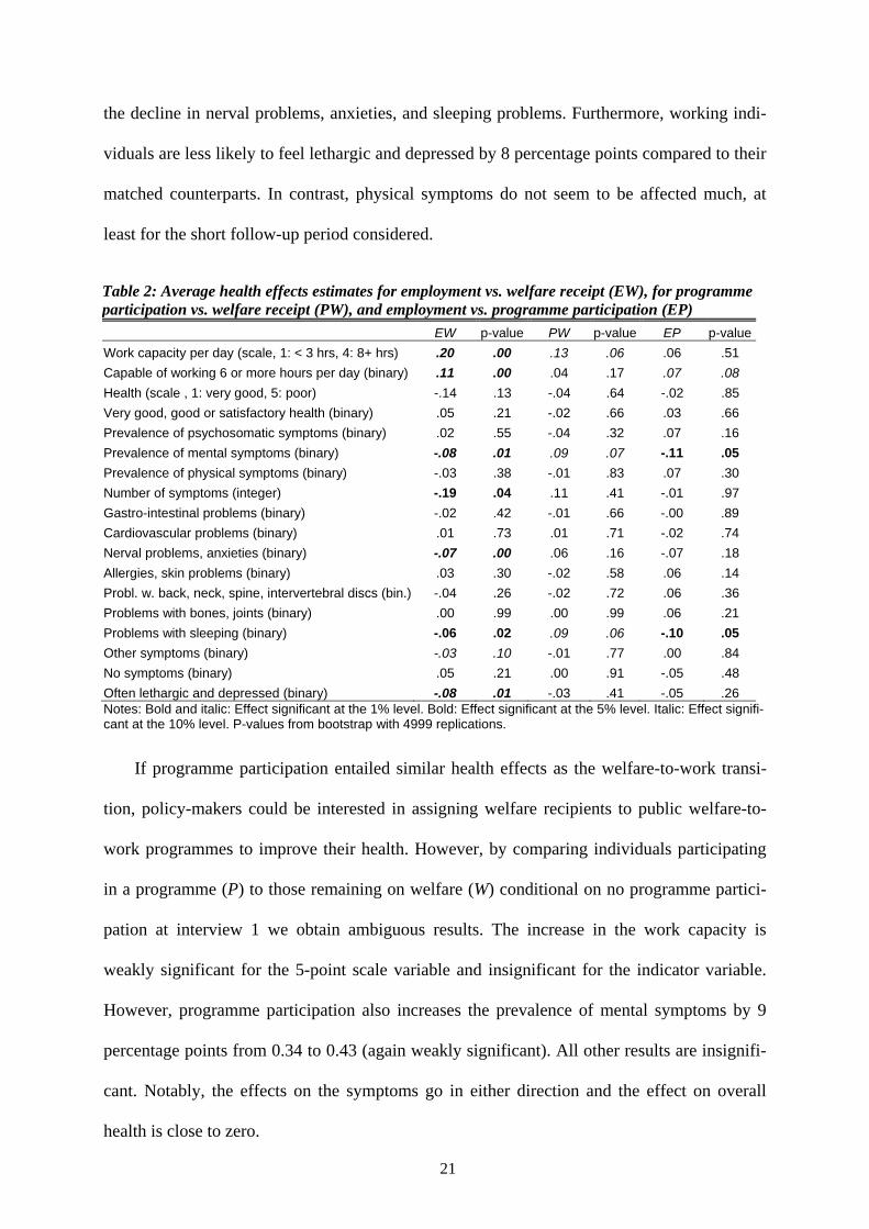
the decline in nerval problems, anxieties, and sleeping problems. Furthermore, working indi-

viduals are less likely to feel lethargic and depressed by 8 percentage points compared to their

matched counterparts. In contrast, physical symptoms do not seem to be affected much, at

least for the short follow-up period considered.

Table 2: Average health effects estimates for employment vs. welfare receipt (EW), for programme participation vs. welfare receipt (PW), and employment vs. programme participation (EP)

EW p-value PW p-value EP p-value

Work capacity per day (scale, 1: < 3 hrs, 4: 8+ hrs) .20 .00 .13 .06 .06 .51 Capable of working 6 or more hours per day (binary) .11 .00 .04 .17 .07 .08 Health (scale , 1: very good, 5: poor) -.14 .13 -.04 .64 -.02 .85 Very good, good or satisfactory health (binary) .05 .21 -.02 .66 .03 .66 Prevalence of psychosomatic symptoms (binary) .02 .55 -.04 .32 .07 .16 Prevalence of mental symptoms (binary) -.08 .01 .09 .07 -.11 .05 Prevalence of physical symptoms (binary) -.03 .38 -.01 .83 .07 .30 Number of symptoms (integer) -.19 .04 .11 .41 -.01 .97 Gastro-intestinal problems (binary) -.02 .42 -.01 .66 -.00 .89 Cardiovascular problems (binary) .01 .73 .01 .71 -.02 .74 Nerval problems, anxieties (binary) -.07 .00 .06 .16 -.07 .18 Allergies, skin problems (binary) .03 .30 -.02 .58 .06 .14 Probl. w. back, neck, spine, intervertebral discs (bin.) -.04 .26 -.02 .72 .06 .36 Problems with bones, joints (binary) .00 .99 .00 .99 .06 .21 Problems with sleeping (binary) -.06 .02 .09 .06 -.10 .05 Other symptoms (binary) -.03 .10 -.01 .77 .00 .84 No symptoms (binary) .05 .21 .00 .91 -.05 .48 Often lethargic and depressed (binary) -.08 .01 -.03 .41 -.05 .26 Notes: Bold and italic: Effect significant at the 1% level. Bold: Effect significant at the 5% level. Italic: Effect signifi-cant at the 10% level. P-values from bootstrap with 4999 replications.

If programme participation entailed similar health effects as the welfare-to-work transi-

tion, policy-makers could be interested in assigning welfare recipients to public welfare-to-

work programmes to improve their health. However, by comparing individuals participating

in a programme (P) to those remaining on welfare (W) conditional on no programme partici-

pation at interview 1 we obtain ambiguous results. The increase in the work capacity is

weakly significant for the 5-point scale variable and insignificant for the indicator variable.

However, programme participation also increases the prevalence of mental symptoms by 9

percentage points from 0.34 to 0.43 (again weakly significant). All other results are insignifi-

cant. Notably, the effects on the symptoms go in either direction and the effect on overall

health is close to zero.

21

Our findings therefore suggest that programme participation does on average not have

such pronounced and unambiguously positive effects on health as employment. This is also

confirmed by the direct comparison of a transition into employment vs. programme participa-

tion conditional on neither being in a programme, nor in employment at interview 1. The in-

crease in the daily work capacity (binary) and the decrease in the prevalence of mental symp-

toms are significant at the 10%- and 5%-level, respectively. Apart from the prevalence of

sleeping problems, all other estimates are rather imprecise, which may be due to the small

sample size.

7 Heterogeneity analysis

In this section, we investigate whether there are subgroups of individuals that particularly

benefit from a transition into employment in terms of health. For this purpose, we estimate the

health effects separately for subsamples defined by the welfare state between the two inter-

views, gender, migrant status, age, education, and initial health.

Table 3 presents the average effects by welfare state. E.g., we evaluate the average health

effects of employment (E) vs. welfare (W) on those actually switching into employment (and

not on the entire population as in Section 5). We denote these parameters as EW|E, indicating

that the average effects are conditional on the state 'employment'. Analogously, EW|W

represents the average health effect on those remaining on welfare. Accordingly, the average

effects of a programme (P) vs. welfare (W) on programme participants and welfare recipients

without programme are PW|P and PW|W. EP|E and EP|P denote the average effects of em-

ployment vs. programme for the employed and programme participants, respectively.

22

Table 3: Average health effect estimates by welfare state for employment vs. welfare (EW), programme vs. welfare (PW), and employment vs. programme (EP)

EW|E EW|P PW|P PW|W EP|E EP|PWork capacity per day (scale, 1: < 3 hrs, 4: 8+ hrs) .09 .26 .16 .13 .06 .07 Capable of working 6 or more hours per day (binary) .02 .16 .05 .04 .08 .07 Health (scale , 1: very good, 5: poor) -.08 -.17 -.15 -.01 -.07 .07 Very good, good or satisfactory health (binary) .01 .07 .07 -.04 .04 -.01 Prevalence of psychosomatic symptoms (binary) .06 .00 -.05 -.03 .10 -.00 Prevalence of mental symptoms (binary) .01 -.12 .03 .10 -.12 -.10 Prevalence of physical symptoms (binary) -.02 -.04 -.05 .00 .07 .05 Number of symptoms (integer) .07 -.33 -.14 .16 .01 -.03 Gastro-intestinal problems (binary) .02 -.04 .01 -.02 -.00 -.01 Cardiovascular problems (binary) .02 .01 -.02 .02 -.01 -.03 Nerval problems, anxieties (binary) -.02 -.11 .04 .07 -.08 -.05 Allergies, skin problems (binary) .04 .03 -.01 -.02 .07 .03 Probl. w. back, neck, spine, intervertebral discs (bin.) -.03 -.05 -.04 -.01 .07 .02 Problems with bones, joints (binary) .03 -.02 -.09 .02 .04 .10 Problems with sleeping (binary) .02 -.11 -.01 .11 -.11 -.08 Other symptoms (binary) -.01 -.03 -.01 .00 -.00 -.01 No symptoms (binary) .04 .05 .06 -.02 -.05 -.05 Often lethargic and depressed (binary) -.05 -.11 -.05 -.02 -.04 -.08 Notes: Bold and italic: Effect significant at the 1% level. Bold: Effect significant at the 5% level. Italic: Effect signifi-cant at the 10% level. P-values from bootstrap with 4999 replications.

Comparing the transition into employment vs. remaining on welfare we find that EW|W

are generally larger and more often significant than EW|E. This implies that the positive

health effects are more pronounced for individuals with less favourable socio-economic char-

acteristics, which more often appear in the group remaining on welfare. Most of the statisti-

cally significant EW|W estimates are similar or slightly higher than the corresponding EW

results. Notably, the effect on the daily work capacity is even stronger. This suggests that

those who would benefit the most from a job placement do actually not get or take this op-

portunity.

All PW|P estimates apart from the positive and weakly significant effect on scale-meas-

ured work capacity are insignificant, which may be partly due to the smaller sample size. The

PW|W results are similar in magnitude and significance to the PW estimates. EP|E and EP|P

estimates for the daily work capacity and mental symptoms go into the same direction as EP

estimates.

23

24

Table 4 reports average health effect estimates for various subgroups defined by gender,

migrant status, age, education, and initial health. Several patterns are worth noting. Most

strikingly, the health effects appear to be much larger for males. The positive effects on men's

overall health and daily work capacity as well as the decrease in the number of symptoms and

the prevalence of mental symptoms and lethargy are large and significant. In contrast, the ef-

fects on women's health are substantially smaller and insignificant in most cases (apart from

the effect on the daily work capacity). This suggests that women's health is much more inert

with respect to the employment state than men's. One potential explanation for this result

might be that males value employment more than females and feel a larger pressure to provide

for themselves and, if existing, their family such that they suffer from higher psychological

distress when remaining on welfare.

The other results in the first panel of Table 4 are less clear-cut, but the positive health ef-

fects of employment seem to be somewhat higher for migrants and prime-age workers in most

cases. The role of education is at best ambiguous. For example, general health is more

strongly increased for individuals with vocational training than for those with a higher educa-

tion (technical school, college, or university), but the converse is true for the daily work ca-

pacity. In contrast, the second panel of Table 4 reveals that there appears to be substantial

effect heterogeneity with respect to initial health. Those reporting poorer overall health in

interview 1 benefit most from a transition into employment as becomes obvious from the

strong increase in the daily work capacity, the substantial decrease in the number of symp-

toms, and the reduced likelihood to face mental symptoms and to feel depressed. As one

would expect from the results discussed so far, health effects are strongest for males with bad

initial health. T-tests indicate that the positive effects on the daily work capacity and the re-

duction in mental symptoms are significantly higher for men with poor health than for those

with better health conditions. In contrast, the health effects for females seem to vary less with

respect to initial health and are not significantly different for those with poor vs. better health.

25

Table 4: Effect heterogeneity of employment vs. welfare receipt in various subgroups

Total Female Male Migrant No migrant 26-40 yrs 41-55 yrs High educa-

tion§ Low educa-

tion+ Work capacity per day (scale, 1: < 3 hrs, 4: 8+ hrs) 0.20 (0.00) 0.14 (0.10) 0.24 (0.00) 0.32 (0.00) 0.22 (0.00) 0.24 (0.00) 0.16 (0.02) 0.30 (0.00) 0.22 (0.00) Capable of working 6 or more hours per day (binary) 0.11 (0.00) 0.09 (0.03) 0.12 (0.00) 0.16 (0.00) 0.10 (0.00) 0.09 (0.00) 0.04 (0.32) 0.15 (0.00) 0.12 (0.02) Health (scale , 1: very good, 5: poor) -0.14 (0.13) -0.05 (0.78) -0.33 (0.00) -0.29 (0.03) -0.18 (0.06) -0.05 (0.65) -0.19 (0.10) -0.06 (0.60) -0.26 (0.00) Very good, good or satisfactory health (binary) 0.05 (0.21) 0.01 (0.84) 0.11 (0.05) 0.03 (0.65) 0.08 (0.07) -0.01 (0.95) 0.06 (0.25) -0.03 (0.70) 0.13 (0.02) Prevalence of psychosomatic symptoms (binary) 0.02 (0.55) 0.02 (0.68) 0.02 (0.70) -0.10 (0.10) 0.04 (0.36) 0.06 (0.28) -0.01 (0.82) 0.13 (0.11) -0.02 (0.71) Prevalence of mental symptoms (binary) -0.08 (0.01) 0.00 (0.98) -0.13 (0.01) -0.09 (0.17) -0.05 (0.26) -0.03 (0.53) -0.05 (0.30) -0.11 (0.04) -0.02 (0.59) Prevalence of physical symptoms (binary) -0.03 (0.38) -0.08 (0.11) 0.00 (0.99) 0.06 (0.40) -0.03 (0.67) -0.04 (0.50) 0.02 (0.77) 0.03 (0.67) -0.04 (0.39) Number of symptoms (integer) -0.19 (0.04) -0.16 (0.30) -0.26 (0.05) -0.38 (0.06) -0.11 (0.43) -0.05 (0.76) -0.15 (0.30) -0.08 (0.59) -0.14 (0.26) Gastro-intestinal problems (binary) -0.02 (0.42) 0.02 (0.73) -0.03 (0.43) -0.07 (0.04) 0.04 (0.36) 0.08 (0.09) -0.03 (0.54) 0.01 (0.74) -0.02 (0.52) Cardiovascular problems (binary) 0.01 (0.73) 0.04 (0.46) -0.02 (0.69) -0.09 (0.09) 0.04 (0.33) 0.01 (0.89) -0.04 (0.27) 0.05 (0.35) -0.02 (0.63) Nerval problems, anxieties (binary) -0.07 (0.00) -0.06 (0.17) -0.09 (0.04) -0.10 (0.17) -0.06 (0.13) -0.07 (0.08) -0.08 (0.07) -0.11 (0.01) -0.06 (0.14) Allergies, skin problems (binary) 0.03 (0.30) 0.02 (0.61) 0.00 (0.93) -0.03 (0.54) 0.02 (0.63) 0.03 (0.52) 0.06 (0.25) 0.06 (0.32) 0.05 (0.33) Probl. w. back, neck, spine, intervertebral discs (bin.) -0.04 (0.26) -0.10 (0.08) -0.01 (0.90) 0.04 (0.54) -0.06 (0.08) -0.01 (0.81) -0.02 (0.69) 0.08 (0.20) -0.07 (0.14) Problems with bones, joints (binary) 0.00 (0.99) -0.05 (0.41) 0.01 (0.90) -0.01 (0.76) -0.01 (0.88) -0.06 (0.15) 0.05 (0.37) -0.10 (0.07) 0.03 (0.49) Problems with sleeping (binary) -0.06 (0.02) 0.00 (1.00) -0.09 (0.03) -0.07 (0.24) -0.05 (0.23) -0.01 (0.75) -0.05 (0.30) -0.04 (0.45) -0.03 (0.45) Other symptoms (binary) -0.03 (0.10) -0.03 (0.19) -0.03 (0.05) 0.02 (0.85) -0.03 (0.05) -0.01 (0.80) -0.03 (0.32) -0.02 (0.40) -0.03 (0.03) No symptoms (binary) 0.05 (0.21) 0.04 (0.51) 0.05 (0.26) -0.04 (0.55) 0.07 (0.11) 0.02 (0.74) 0.04 (0.45) 0.01 (0.90) 0.03 (0.63) Often lethargic and depressed (binary) -0.08 (0.01) -0.03 (0.62) -0.11 (0.01) -0.08 (0.24) -0.06 (0.24) -0.10 (0.01) -0.11 (0.08) -0.07 (0.24) -0.10 (0.01) Observations 1378 680 698 415 963 557 458 411 779 Common support 94% 92% 91% 76% 92% 88% 83% 87% 92% Notes: Average health effect estimates per subgroup. p-values based on 999 bootstrap replications in parentheses. §: technical school, college or university. +: vocational training. Shaded figures: Effect differences across subgroups are significant at the 5% level (t-tests). Bold and italic: Effect significant at the 1% level. Bold: Effect significant at the 5% level. Italic: Effect significant at the 10% level.

- To be continued -

26

Table 4: Effect heterogeneity of employment vs. welfare receipt in various subgroups (continued)

Total

Very good to satisfactory

health Less than satisfy.

health

Females, very good to

satisfy. health

Females, less than satisfy.

health

Males, very good to

satisfy. health

Males, less than

satisfy. health Work capacity per day (scale, 1: < 3 hrs, 4: 8+ hrs) 0.20 (0.00) 0.17 (0.00) 0.35 (0.00) 0.18 (0.04) 0.25 (0.04) 0.19 (0.00) 0.29 (0.02) Capable of working 6 or more hours per day (binary) 0.11 (0.00) 0.07 (0.00) 0.17 (0.00) 0.12 (0.00) 0.04 (0.58) 0.02 (0.41) 0.19 (0.01) Health (scale , 1: very good, 5: poor) -0.14 (0.13) -0.14 (0.03) -0.26 (0.11) -0.09 (0.31) -0.26 (0.11) -0.15 (0.12) -0.44 (0.00) Very good, good or satisfactory health (binary) 0.05 (0.21) 0.06 (0.10) 0.05 (0.41) 0.03 (0.54) 0.06 (0.31) 0.05 (0.22) 0.13 (0.13) Prevalence of psychosomatic symptoms (binary) 0.02 (0.55) 0.04 (0.30) 0.01 (0.86) -0.01 (0.84) -0.06 (0.49) 0.04 (0.33) 0.02 (0.83) Prevalence of mental symptoms (binary) -0.08 (0.01) 0.01 (0.63) -0.18 (0.01) 0.01 (0.75) -0.10 (0.25) 0.00 (0.90) -0.20 (0.02) Prevalence of physical symptoms (binary) -0.03 (0.38) -0.01 (0.82) -0.06 (0.33) -0.03 (0.67) -0.09 (0.32) 0.09 (0.11) 0.06 (0.44) Number of symptoms (integer) -0.19 (0.04) 0.02 (0.79) -0.51 (0.00) -0.10 (0.42) -0.51 (0.06) 0.20 (0.07) -0.29 (0.23) Gastro-intestinal problems (binary) -0.02 (0.42) 0.03 (0.20) -0.04 (0.41) 0.03 (0.51) -0.06 (0.40) 0.06 (0.12) -0.14 (0.01) Cardiovascular problems (binary) 0.01 (0.73) -0.02 (0.42) 0.03 (0.55) -0.05 (0.27) 0.07 (0.43) -0.01 (0.82) 0.01 (0.92) Nerval problems, anxieties (binary) -0.07 (0.00) -0.01 (0.51) -0.14 (0.04) -0.02 (0.61) -0.13 (0.18) 0.00 (0.88) -0.12 (0.11) Allergies, skin problems (binary) 0.03 (0.30) 0.04 (0.15) 0.06 (0.46) 0.03 (0.36) 0.02 (0.84) 0.01 (0.58) 0.05 (0.67) Probl. w. back, neck, spine, intervertebral discs (bin.) -0.04 (0.26) -0.02 (0.62) -0.08 (0.22) -0.03 (0.58) -0.11 (0.28) 0.09 (0.06) 0.08 (0.37) Problems with bones, joints (binary) 0.00 (0.99) 0.01 (0.71) -0.07 (0.26) -0.06 (0.14) -0.16 (0.05) 0.09 (0.06) 0.00 (0.98) Problems with sleeping (binary) -0.06 (0.02) 0.02 (0.52) -0.19 (0.00) 0.00 (0.91) -0.10 (0.21) 0.00 (0.98) -0.15 (0.02) Other symptoms (binary) -0.03 (0.10) -0.03 (0.07) -0.04 (0.09) -0.02 (0.39) -0.02 (0.32) -0.02 (0.72) -0.01 (0.69) No symptoms (binary) 0.05 (0.21) 0.04 (0.39) 0.00 (0.92) 0.04 (0.57) 0.03 (0.50) 0.02 (0.75) -0.04 (0.48) Often lethargic and depressed (binary) -0.08 (0.01) -0.05 (0.11) -0.11 (0.08) -0.09 (0.04) -0.09 (0.32) -0.05 (0.16) -0.14 (0.04) Observations 1378 765 613 386 294 379 319 common support 94% 93% 85% 87% 84% 86% 89% Notes: Average health effect estimates per subgroup. p-values based on 999 bootstrap replications in parentheses. Shaded figures: Effect differences between subgroups are significant at the 5% level (t-tests). Bold and italic: Effect significant at the 1% level. Bold: Effect significant at the 5% level. Italic: Effect significant at the 10% level.

27

8 Robustness checks

8.1 Instrumental-variable-based identification and estimation

As at least a subset of identifying assumptions underlying any causal analysis is not test-

able, it would be valuable to have available alternative identification strategies that appear to

be equally credible. Ideally, both strategies should lead to similar results, or at least not con-

tradict each other. Below we argue that there exists an instrumental variable (IV) strategy that

also identifies the health effects of employment vs. remaining on welfare.

Identification based on instrumental variables hinges on the availability of a variable that

is correlated with the welfare state but has no direct effect on the outcome, an instrument. We

argue that the indicator variable 'possession of a driver's licence' is, at least conditional on

other observed factors, a valid instrument for the welfare-to-employment transition. It is quite

intuitive that the possession of a driver's license has a positive correlation with the probability

to find work. Firstly, a driver's license increases the mobility and the likelihood to accept jobs

that are more distant from home. Secondly, it represents a form of human capital that might

be substantial for jobs targeted at low-educated individuals (e.g., carrier services). Indeed, the

data show a positive correlation between license possession and transition into employment,

significant at the 5 % level. The variation in the instrument is quite substantial, as only 62% of

the individuals in the sample have a driver's license, which is more than 10% less than the

German average.12

12 According to the survey "Typologie der Wünsche 2006/2007" which was conducted in 2006/07 and is representative for the German population older than 13. For details, see http://de.statista.org/statistik/diagramm/studie/32090/umfrage /besitz-pkw-fuehrerschein/#info. The difference is plausible given that we observe a particular share of the German population that is poorer, less educated, and less attached to the labour market than the average.

28

However, for the instrument to be 'valid' it must be plausible that there are no direct ef-

fects of license possession on health. This may be challenged in the case of a recently ob-

tained driver's license, which abruptly increases mobility and the possibility to extend social

contacts, and might affect mental health for this reason. It, therefore, seems advisable to ex-

clude individuals that obtained their licenses rather recently. Even though the data do not

contain the licence’s issue date, they contain information on the age at which individuals usu-

ally receive their driver's license. The share of license possessors conditional on age increases

steadily up to the age of 26 when it reaches its peak (roughly 75%) and declines slowly after-

wards to 62% for the age group 60-65. This suggests that increases below 26 are mainly

growth driven, i.e., they are caused by individuals who recently passed the driving test. The

moderate declines above 26 are most likely due to cohort effects as older generations (and

among them, particularly women) are less likely to ever obtain a driver's license. To reinforce

the plausibility of the instrument, we therefore exclude individuals younger than 26.

The instrument validity (exclusion restriction) is also violated if some characteristics are

jointly related to license possession and health. Two potential confounders already mentioned

are age (cohort effects) and gender (role models). Furthermore, the instrument is correlated

with the socio-economic status (income, wealth, education, and profession) if wealthier indi-

viduals are more inclined to invest in a driver’s license.13 We would also expect that marital

status, household composition and the presence of children are joint determinants, as families

might prefer to invest in private mobility whereas single households might not. Urbanization

and the availability of public transport as substitute for private mobility are further potential

determinants. Social networks, milieu, and migration background might also shape prefer-

13 This argument is supported by the results in "Typologie der Wünsche 2006/2007", where 84.1% of the highest income group (4000 EUR and more per month), but only 54.2% of the lowest income group (up to 499 EUR) possess a driver’s license.

29

ences concerning driving. Effort and ability reflect the non-monetary cost of passing the

driving test. Finally, it seems plausible that the possession of a driver's license varies with

initial health and disability status.

It can be reasonably argued that these factors are also related to health in one or the other

way. This implies that the instrument is only valid conditional on the aforementioned con-

founders. Our data allow us to either directly observe or to proxy these factors potentially re-

lated to the instrument and the outcomes. We, therefore, believe that our instrument is valid

conditional on observed characteristics. Descriptive statistics for potential IV confounders are

provided in the internet appendix.

Under some conditions, the IV approach identifies the so-called local average treatment

effect (LATE), which is in our case the mean effect of employment on health among those

individuals not working without driver's license and working with a licence. It is thus the

average causal effect for those who comply in the sense that they switch from welfare to em-

ployment if they are provided with a driver's license. If the health effects are heterogeneous,

one could expect the LATE to differ from the other causal effects presented in the previous

sections, as it refers to a different population, namely the compliers. See Imbens and Angrist

(1994) and Angrist, Imbens, and Rubin (1996) for an in depth discussion of the LATE pa-

rameter and its identifying assumptions.

For LATE estimation conditional on observed characteristics we use a semi-parametric

method suggested by Frölich (2007) which is outlined in the internet appendix. This method

contains two matching steps for which we use the same algorithm as for the estimates pre-

sented in Section 6. The LATE estimates are reported in Table A.2 of Appendix B along with

quantiles of the effects' distributions obtained from 4999 bootstrap replications and the esti-

mates of the intention to treat (ITT) effects. Due to the small proportion of compliers (roughly

15%) the LATE estimates are rather imprecise (none is statistically different from zero at the

10% level) and should not be taken at face value. We merely use them to check the robustness

of the matching estimates. In fact, each of the latter is included in the 90% confidence interval

of the respective LATE estimate. Therefore, we do not find contradictory evidence to the

matching results based on the CIA.

8.2 Parametric regression

As a further robustness check, we estimate the effects parametrically using OLS for the

health and work capacity measured by scales and probit specifications for the binary health

outcomes. For each comparison we regress the health outcomes on a binary transition indica-

tor (e.g., 1 for employment and 0 for welfare) and on all variables included in the respective

propensity score specification. The parametric methods neither account for effect heterogene-

ity, nor for non-linearities between the welfare state, the covariates, and the health outcomes.

Table A.3 in Appendix B presents the effect estimates and analytical p-values. For the bi-

nary outcomes, the health effects are evaluated at the respective sample's mean characteristics

of . The employment transition's effects on the prevalence of mental symptoms and feel-

ings of depression are negative while the daily work capacity is increased. Most of the effect

estimates related to programme participation are again statistically insignificant. Overall, we

find effects very similar to the ones based on matching. Thus, we conclude that the parametric

results, albeit prone to potential specification bias, support our main results.

X

9 Conclusion

We estimate the effects of a transition from welfare to employment or to welfare-to-work

programmes on various physical and mental health outcomes by analysing a combination of

exceptionally informative survey and administrative data on German welfare recipients that

have been linked to regional information and characteristics of employment offices. The rich-

ness of the data as well as the possibility to condition on the pre-transition states of the out-

30

31

come variables allows us to control for the relevant confounding factors in our estimation

based on semi-parametric propensity score matching. We also use semi-parametric IV esti-

mators and parametric regressions to check the robustness of the matching estimates and find

no contradictory results.

The results suggest that employment increases health in general and mental health in par-

ticular, as evidenced by substantial decreases in the prevalence of mental symptoms and

feelings of depression, and an improved daily work capacity. These effects are mainly driven

by males, suggesting that women's health is relatively inert with respect to the employment

state. Moreover, welfare recipients with less favourable characteristics, in particular with bad

initial health, seem to be more likely to benefit than the better risks. Effects are most pro-

nounced for males with bad initial health. Therefore, it seems that at least some of the adverse

effects on health that have been documented in the literature on job displacement (e.g., Kuhn,

Lalive, and Zweimüller, 2007, Browning, Dano, and Heinesen, 2006) are potentially reversi-

ble.

In contrast, the effect of programme participation is ambiguous and most effect estimates

are not significantly different from zero. Thus, keeping unemployed individuals 'busy' in wel-

fare-to-work programmes ceteris paribus entails poorer health states than a placement into

employment, which might be crucial for future employability. From this perspective, a 'work

first' approach rather than extensive use of welfare-to-work programmes seems to be in the

interest of both policy-makers and welfare recipients.

32

References

Abadie, A., and G. W. Imbens (2006): "Large Sample Properties of Matching Estimators for Average Treatment Effects", Econometrica, 74, 235-267.

Abadie, A., and G. W. Imbens (2008): "On the Failure of the Bootstrap for Matching Estimators", Econometrica, 76, 1537-1557.

Angrist, J. D., G. W. Imbens, and D. B. Rubin (1996): "Identification of Causal Effects Using Instrumental Vari-ables", Journal of the American Statistical Association, 91, 444–472.

Baker, M., M. Stabile, and C. Deri: "What Do Self-Reported, Objective, Measures of Health Measure?", The Journal of Human Resources, 39, 1067-1093.

Benítez-Silva, H., M. Buchinsky, H. M. Chan, S. Cheidvasser, and J. Rust (2004): "How large is the bias in self-reported disability?", Journal of Applied Econometrics, 19, 649-670.

Björklund, A., and T. Eriksson (1998): "Unemployment and mental health: evidence from research in the Nordic countries", Scandinavian Journal of Social Welfare, 7, 219-235.

Böckerman, P., and P. Ilmakunnas (2009): "Unemployment And Self-Assessed Health: Evidence From Panel Data", Health Economics, 18, 161–179.

Boothroyd, R. A., and D. Olufokunbi (2001): "Leaving theWelfare Rolls: The Health and Mental Health Status of Current and Former Welfare Recipients", Mental Health Services Research, 3, 119- 128.

Bound, J. (1991): "Self-Reported Versus Objective Measures of Health in Retirement Models", The Journal of Human Resources, 26, 106-138.

Browning, M., A. M. Dano, and E. Heinesen (2006): "Job displacement and stress-related health outcomes", Health Economics, 15, 1061–1075.

Burgard, S., J. Brand, and J. House (2005): "Causation and Selection in the Relationship of Job Loss to Health in the United States", mimeo, University of Michigan.

Butterworth, P., T. Crosier, and B. Rodgers (2004): "Mental Health Problems, Disability and Income Support Receipt: A Replication and Extension Using the HILDA Survey", Australian Journal of Labour Economics, 7, 151-174.

Byrne, C., G. Browne, J. Roberts, B. Ewart, M. Schuster, J. Underwood, S. Flynn-Kingston, K. Rennick, B. Bell, A. Gafni, S. Watt, Y. Ashford, and E. Jamieson (1998): "Surviving social assistance: 12-month prevalence of depression in sole-support parents receiving social assistance", Canadian Medical Association Journal, 158, 881-888.

Coiro, M. J. (2001): "Depressive symptoms among women receiving welfare", Women Health, 32, 1-23.

Danziger, S. K., M. J. Carlson, and J. R. Henly (2001): "Post-welfare employment and psychological well-be-ing", Women Health, 32, 47-78.

Danziger, S. K., A. Kalil, and N. J. Anderson (2000): "Human Capital, Physical Health, and Mental Health of Welfare Recipients: Co-occurrence and Correlates", Journal of Social Issues, 56, 635-654.

Dehejia, R. H., and S. Wahba (2002): "Propensity-Score-Matching Methods for Nonexperimental Causal Stud-ies", Review of Economics and Statistics, 84, 151-161.

33

Eaton, W. W., C. Muntaner, G. Bovasso, and C. Smith (2001): "Socioeconomic Status and Depressive Syn-drome: The Role of Inter- and Intra-generational Mobility, Government Assistance, and Work Environment", Journal of Health and Social Behavior, 42, 277-294.

Ensminger, M. E. (1995): "Welfare and Psychological Distress: A Longitudinal Study of African America Urban Mothers", Journal of Health and Social Behavior, 36, 346-359.

Ensminger, M. E., and H. S. Juon (2001): "The influence of patterns of welfare receipt during the child-rearing years on later physical and psychological health", Women Health, 32, 25-46.

Frijters, P., J. P. Haisken-DeNew, and M. A. Shields (2005): "The causal effect of income on health: Evidence from German reunification", Journal of Health Economics, 24, 997-1017.

Frölich, M. (2007): "Nonparametric IV estimation of local average treatment effects with covariates", Journal of Econometrics, 139, 35-75.

Gallo, W. T., E. H. Bradley, M. Siegel, and S. V. Kasl (2000): "Health Effects of Involuntary Job Loss Among Older Workers: Findings From the Health and Retirement Survey", Journal of Gerontology, 55B, 131-140.

Gallo, W. T., H. M. Teng, T. A. Falba, S. V. Kasl, H. M. Krumholz, and E. H. Bradley (2006): "The impact of late career job loss on myocardial infarction and stroke: a 10 year follow up using the health and retirement survey", Occupational and Environmental Medicine, 63, 683-687.

Gerfin, M., and M. Lechner (2002): "A Microeconometric Evaluation of the Active Labour Market Policy in Switzerland", The Economic Journal, 112, 854-893.

Gravelle, H., and M. Sutton (2009): "Income, Relative Income, and Self-Reported Health In Britain 1979-2000", Health Economics, 18, 125-145.

Grogger, J., and L. Karoly (2005): "Welfare Reform: Effects of a Decade of Change", Harvard University Press.

Heckman, J. J., R. LaLonde, and J. A. Smith (1999): "The Economics and Econometrics of Active Labor Market Programs", in: O. Ashenfelter and D. Card (eds.), Handbook of Labour Economics, 3, 1865-2097, Amster-dam: North-Holland.

Imbens, G. W. (2004): "Nonparametric Estimation of Average Treatment Effects Under Exogeneity: A Review", The Review of Economics and Statistics, 86, 4-29.

Imbens, G. W., and J. D. Angrist (1994): "Identification and Estimation of Local Average Treatment Effects," Econometrica, 62, 467-475.

Jayakody, R., S. K. Danziger, and H. Pollack (2000): "Welfare Reform, Substance Use, and Mental Health", Journal of Health Politics, Policy and Law, 25, 623-652.

Jin, R. L., C. P. Shah, and T. J. Svoboda (1997): "The Impact of Unemployment on Health: A Review of the Evidence", Journal of Public Health Policy, 18, 275-301.

Joffe, M. M., T. R. Ten Have, H. I. Feldman, and S. Kimmel (2004): "Model Selection, Confounder Control, and Marginal Structural Models", The American Statistician, 58-4, 272-279.

Kalil, A., C. E. Born, J. Kunz, and P. J. Caudill (2001): "Life Stressors, Social Support, and Depressive Symp-toms Among First-TimeWelfare Recipients", American Journal of Community Psychology, 29, 355-369.

Kalwij, A., and F. Vermeulen (2008): "Health and labour force participation of older people in Europe: What do objective health indicators add to the analysis?", Health Economics, 17, 619-638.

34

Kluve, J. (2006): "The Effectiveness of European Active Labor Market Policy", IZA Discussion Paper 2018, Institute for the Study of Labor (IZA), Bonn.

Kovess, V., S. Gysens, R. Poinsard, P. F. Chanoit, and S. Labarte (2001): "Mental health and use of care in peo-ple receiving a French social benefit", Social psychiatry and psychiatric epidemiology, 34, 588-594.

Kreider, B., and J. V. Pepper (2007): "Disability and Employment: Reevaluating the Evidence in Light of Re-porting Errors", Journal of the American Statistical Association, 102, 432-441.

Kreider, B., and J. V. Pepper (2008): "Inferring disability status from corrupt data", Journal of Applied Econo-metrics, 23, 329-349.

Kuhn, A., R. Lalive, and J. Zweimüller (2007): "The Public Health Costs of Unemployment", Cahiers de Re-cherches Economiques du Département d'Econométrie et d'Economie politique 07.08, Université de Lausanne.

LaLonde, R. J. (2003): "Employment and Training Programs", in M. Feldstien and R. Moffitt (Eds.): "Means Tested Transfer Programs in the U.S.", Chicago: University of Chicago Press for the National Bureau of Economic Research.

Lechner, M., R. Miquel, and C. Wunsch (2009): "Long-Run Effects of Public Sector Sponsored Training in West Germany", Journal of the European Economic Association, forthcoming.

Lindeboom, M., and E. van Doorslaer (2004): "Cut-point shift and index shift in self-reported health", Journal of Health Economics, 23, 1083-1099.

Llena-Nozal, A., M. Lindeboom, and F. Portrait (2004): " The effect of work on mental health: does occupation matter?", Health Economics, 13, 1045-1062.

MacKinnon, J. G. (2006). "Bootstrap Methods in Econometrics", The Economic Record, 82, 2-18.

Mathers, C. D., and D. J. Schofield (1998): " The health consequences of unemployment: the evidence", The Medical Journal of Australia, 168, 178-182.

Maurer, J., R. Klein, and F. Vella (2007): "Subjective Health Assessments and Active Labor Market Participa-tion of Older Men: Evidence from a Semiparametric Binary Choice Model with Nonadditive Correlated Indi-vidual-Specific Effects", IZA Discussion Paper No. 3257.

Mulatu, S., and C. Schooler (2002): "Causal Connections between Socio-Economic Status and Health: Recipro-cal Effects and Mediating Mechanisms", Journal of Health and Social Behavior, 43, 22-41.

Olson, K., and L. Pavetti (1996): "Personal and family challenges to the successful transition from welfare to work", Washington, DC, Urban Institute.

Smith, J. P. (2007): "The Impact of Socioeconomic Status on Health over the Life-Course", The Journal of Hu-man Resources, 42, 739-764.

Rosenbaum, P., and D. Rubin (1983): "The Central Role of the Propensity Score in Observational Studies for Causal Effects", Biometrika, 70, 41-55.

Rubin, D. B. (1979): "Using Multivariate Matched Sampling and Regression Adjustment to Control Bias in Observational Studies", Journal of the American Statistical Association, 74, 318-328.

Van Doorslaer, E., and A. M. Jones (2003): "Inequalities in self-reported health: validation of a new approach to measurement", Journal of Health Economics, 22, 61-87.

Appendix A: Technical details of the matching estimator used

Table A.1: A matching protocol for the estimation of a counterfactual outcome and the effects

Step 1 Specify a reference distribution defined by X. Step 2 Pool the observations forming the reference distribution and the participants in the respective period. Code an

indicator variable D, which is 1 if the observation belongs to the reference distribution. All indices, 0 or 1, used below relate to the actual or potential values of D.

Step 3 Specify and estimate a binary probit for ( ) : ( 1 | )p x P D X x= = = Step 4 Restrict sample to common support: Delete all observations with probabilities larger than the smallest maximum

and smaller than the largest minimum of all subsamples defined by D. Step 4 Estimate the respective (counterfactual) expectations of the outcome variables.

Standard propensity score matching step (multiple treatments) a-1) Choose one observation in the subsample defined by D=1 and delete it from that pool. b-1) Find an observation in the subsample defined by D=0 that is as close as possible to the one chosen in step a-1) in terms of ( ),p x x . 'Closeness' is based on the Mahalanobis distance. Do not remove that observation, so that it can be used again. c-1) Repeat a-1) and b-1) until no observation with D=1 is left. Exploit thick support of X to increase efficiency (radius matching step) d-1) Compute the maximum distance (d) obtained for any comparison between a member of the reference distri-bution and matched comparison observations. a-2) Repeat a-1). b-2) Repeat b-1). If possible, find other observations in the subsample of D=0 that are at least as close as R * d to the one chosen in step a-2) (to gain efficiency). Do not remove these observations, so that they can be used again. Compute weights for all chosen comparisons observations that are proportional to their distance. Normal-ise the weights such that they add to one. c-2) Repeat a-2) and b-2) until no participant in D=1 is left. d-2) For any potential comparison observation, add the weights obtained in a-2) and b-2). Exploit double robustness properties to adjust small mismatches by regression e) Using the weights btained in d-2), run a weighted linear regression of the outcome variable on the variables used to define the distance (and an intercept).

o

f-1) Predict the potential outcome of every observation using the coefficients of this regression: . 0 ( )iy x 0ˆ ( )iy x

f-2) Estimate the bias of the matching estimator for 0( | 1)E Y D = as: 0

35

001

1 01

ˆˆ 1( 0) ( )1( 1) ( )=

==−∑

Ni

i

D w y xD y xN N

.

g) Using the weights obtained by weighted matching in d-2), compute a weighted mean of the outcome variables in D=0. Subtract the bias from this estimate to get 0( | 1)E Y D = .

Step 5 Repeat Steps 2 to 4 with the nonparticipants playing the role of participants before. This gives the desired esti-mate of the counterfactual nonparticipation outcome.

Step 6 The difference of the potential outcomes is the desired estimate of the effect with respect to the reference distri-bution specified in Step 1.

( )iw x

The parameter used to define the radius for the distance-weighted radius matching (R) is

set to 90%. This value refers to the distance of the worst match in a one-to-one matching and

is defined in terms of the propensity score. Different values for R are checked in the sensitiv-

ity analysis in Lechner, Miquel, and Wunsch (2009). The results were robust as long as R did

not become 'too large'.

Appendix B: Estimates of the robustness checks

Table A.2: LATE estimates

LATE 2.5th percentile

5th percentile

95th percentile

97.5th percentile

ITT estimate

Work capacity per day (scale, 1: < 3 hrs, 4: 8+ hrs) .23 -.76 -.53 1.19 1.40 .03 Capable of working 6 or more hours per day (binary) .10 -.29 -.21 .58 .69 .02 Health (scale , 1: very good, 5: poor) .37 -1.18 -.91 1.54 1.91 .06 Very good, good or satisfactory health (binary) -.11 -.61 -.47 .51 .63 -.02 Prevalence of psychosomatic symptoms (binary) -.51 -.98 -.84 .23 .34 -.08 Prevalence of mental symptoms (binary) .03 -.65 -.50 .40 .51 .00 Prevalence of physical symptoms (binary) -.09 -.89 -.66 .37 .47 -.01 Number of symptoms (integer) -.80 -2.54 -2.12 .53 .77 -.12 Gastro-intestinal problems (binary) -.04 -.65 -.54 .30 .38 -.01 Cardiovascular problems (binary) -.56 -1.18 -.99 .05 .13 -.08 Nerval problems, anxieties (binary) -.07 -.62 -.49 .32 .42 -.01 Allergies, skin problems (binary) -.09 -.57 -.45 .44 .58 -.01 Probl. w. back, neck, spine, intervertebral discs (bin.) -.40 -1.58 -1.24 .02 .10 -.06 Problems with bones, joints (binary) .24 -.13 -.06 .88 1.09 .04 Problems with sleeping (binary) .05 -.53 -.38 .46 .56 .01 Other symptoms (binary) -.08 -.41 -.33 .05 .08 -.01 No symptoms (binary) .11 -.31 -.24 .57 .71 .02 Often lethargic and depressed (binary) .19 -.27 -.17 .59 .73 .03 Notes: Bold and italic: Effect significant at the 1% level. Bold: Effect significant at the 5% level. Italic: Effect signifi-cant at the 10% level. Quantiles from bootstrap with 4999 replications. Table A.3: Parametric estimates            

E-W P-W E-P Effect p-value Effect p-value Effect p-value

Work capacity per day (scale, 1: < 3 hrs, 4: 8+ hrs) .18 .00 .16 .00 .08 .18 Capable of working 6 or more hours per day (binary) .10 .00 .08 .01 .03 .11 Health (scale , 1: very good, 5: poor) -.18 .00 -.07 .28 -.12 .18 Very good, good or satisfactory health (binary) .07 .06 .01 .79 .07 .20 Prevalence of psychosomatic symptoms (binary) .03 .43 -.06 .12 .08 .12 Prevalence of mental symptoms (binary) -.06 .08 .03 .46 -.11 .03 Prevalence of physical symptoms (binary) -.02 .58 -.03 .48 .04 .47 Number of symptoms (integer) -.03 .20 -.03 .25 .00 .94 Gastro-intestinal problems (binary) .01 .50 -.01 .52 .02 .43 Cardiovascular problems (binary) .01 .72 .01 .79 -.02 .47 Nerval problems, anxieties (binary) -.07 .00 .02 .49 -.09 .02 Allergies, skin problems (binary) .01 .76 -.02 .38 .03 .27 Probl. w. back, neck, spine, intervertebral discs (bin.) -.02 .59 .00 .99 .05 .37 Problems with bones, joints (binary) -.01 .68 -.04 .19 .04 .37 Problems with sleeping (binary) -.02 .54 .03 .45 -.07 .10 Other symptoms (binary) -.02 .04 -.01 .23 -.01 .51 No symptoms (binary) .03 .20 .03 .25 .00 .94 Often lethargic and depressed (binary) -.08 .00 -.04 .13 -.06 .10 Notes: Average effects on the binary outcomes are evaluated at the mean characteristics of X . Bold and italic: Effect significant at the 1% level. Bold: Effect significant at the 5% level. Italic: Effect significant at the 10% level.

36