Does income inequality raise aggregate...

Journal of Development EconomicsŽ .Vol. 61 2000 417–446

www.elsevier.comrlocatereconbase

Does income inequality raise aggregate saving?

Klaus Schmidt-Hebbel a,), Luis Serven b,1´a Central Bank of Chile, Agustinas 1180, Santiago, Chile

b The World Bank, 1818 H Street, NW, Washington, DC 20433, USA

Abstract

This paper reviews analytically and empirically the links between income distributionand aggregate saving. Consumption theory brings out a number of direct channels throughwhich income inequality can affect overall household saving — positively in most cases.However, recent political-economy theory points toward indirect, negative effects ofinequality — through firm investment and public saving — on aggregate saving. Ontheoretical grounds, the sign of the saving–inequality link is therefore ambiguous. Thispaper presents new empirical evidence on the relationship between income distribution andaggregate saving based on a new and improved income distribution database for bothindustrial and developing countries. The empirical results, using alternative inequality andsaving measures and various econometric specifications on both cross-section and paneldata, provide no support for the notion that income inequality has any systematic effect onaggregate saving. These findings are consistent with the theoretical ambiguity. q 2000Elsevier Science B.V. All rights reserved.

PACS: E21; D31Keywords: Saving; Inequality; Income distribution

1. Introduction

The theoretical relation between saving and income distribution has receivedattention both in the historical growth literature and more recent neoclassicalconsumption theory. In fact, the link between the functional distribution of income

) Corresponding author. Tel.: q56-2-670-2586; fax: q56-2-670-2853.Ž .E-mail addresses: [email protected] K. Schmidt-Hebbel , [email protected]

Ž .L. Serven .´1 Tel.: q1-202-473-7451; fax: q1-202-522-2119.

0304-3878r00r$ - see front matter q 2000 Elsevier Science B.V. All rights reserved.Ž .PII: S0304-3878 00 00063-8

( )K. Schmidt-Hebbel, L. SerÕenrJournal of DeÕelopment Economics 61 2000 417–446´418

Ž . Žand saving and growth is at the heart of the neoclassical growth model Solow,. Ž1956 as well as neo-Keynesian growth models Lewis, 1954; Kaldor, 1957;

.Pasinetti 1962 . In more recent neoclassical consumption theory, the focus is onthe links between personal distribution of income and aggregate saving as a resultof consumer heterogeneity in regard to endowments or institutional constraintsŽ . Ž .see Deaton, 1992 for a discussion . Most but not all of the mechanisms pointedout by the above mentioned theories suggest positive direct effects of incomeinequality on overall personal saving. However, recent political-economy researchbrings out negative indirect links from inequality — through investment, growth,

Žor public saving — to aggregate saving e.g., Dornbusch and Edwards, 1991;.Persson and Tabellini, 1994; Alesina and Perotti, 1996 . Taken together, these two

strands of the literature imply that the overall impact of inequality on aggregatesaving is theoretically ambiguous and can only be assessed empirically.

Most of the empirical literature on the links between personal income inequalityand personal saving based on cross-section micro data suggest a positive relation

Ž .between them e.g., Bunting, 1991; Dynan et al., 1996 . In turn, the evidence fromŽ .aggregate typically cross-country data is more mixed. Some studies also find

positive and significant effects of personal income inequality on aggregate savingŽ . ŽSahota, 1993; Cook, 1995; Hong, 1995 , but other studies do not Della Valle and

.Oguchi, 1976; Musgrove, 1980; Edwards, 1996 . Reconciling these conflictingresults is difficult because empirical studies based on macro data use differentsamples and specifications, different measures of saving and inequality and, inmost cases, income distribution information of questionable quality.

This paper reexamines the empirical evidence from macro data on the linksbetween the distribution of personal income and aggregate saving, controlling forrelevant saving determinants. It provides an encompassing framework and arobustness check for previous empirical studies, and extends them in five dimen-

Ž . Ž .sions: i testing alternative saving specifications; ii using alternative inequalityŽ . Ž .and saving measures; iii making use of newer, better and larger databases; iv

conducting estimations jointly and separately for industrialized and developingŽ .countries; and v applying various estimation techniques on both cross-country

and panel data. On the whole, we do not find any consistent effect of incomeinequality on aggregate saving — a result that is consistent with the theoreticalambiguity.2

The paper is organized as follows. Section 2 provides a brief literature surveyon the links between income distribution and saving determination. Section 3reviews previous empirical studies of the impact of income distribution on saving.

2 This paper thus extends significantly, along several dimensions, preliminary findings reported inŽ .Schmidt-Hebbel and Serven 1999 which also showed little effects of income distribution on saving.´

Such provisional conclusion is considerably strengthened in this article based on an expanded database,presenting results that exploit both the medium and long time frequencies of the data, and performingsystematic robustness tests over alternative specifications and estimation techniques.

( )K. Schmidt-Hebbel, L. SerÕenrJournal of DeÕelopment Economics 61 2000 417–446´ 419

A description of the large database on inequality and saving, used in this paper,follows. Section 5 presents new econometric evidence and Section 6 concludes.

2. Income distribution and saving: a brief survey

Aggregate saving is the outcome of individual saving efforts by heterogeneousmembers of different classes of savers. Heterogeneity may be due to the fact thatdifferent individuals determine their consumptionrsaving plans according to dif-

Ž .ferent objectives i.e., their preferences are not identical . Even if all individualspossess identical preferences, their behavior may differ because they face different

Ž .institutional constraints e.g., in their access to borrowing . Heterogeneity is ofcourse important because when agents are dissimilar, the aggregate levels of thosevariables that are relevant for individual saving decisions are typically notsufficient to determine aggregate saving — the latter also depends on thedistribution of such variables across individual savers.3 However, even if allagents share the same preferences and face identical constraints, distribution still

Ž .matters as long as agents’ common decision rule for saving is not linear in therelevant variables.4

Next, we review briefly the literature on saving and income distribution,analyzing the channels through which different forms of income distribution affect

Ž .aggregate saving. We examine four topics: i links between saving and theŽ .functional distribution of income; ii links between saving and the personal

Ž .distribution of income; iii implications of precautionary saving and borrowingŽ .constraints for distribution and saving; and iv indirect effects of distribution on

saving.Ž .The link between the functional distribution of income and saving and growth

Ž .is at the heart of the neoclassical growth model Solow, 1956 , as well as theŽ . Ž .neo-Keynesian growth models of Lewis 1954 , Kaldor 1957 and Pasinetti

Ž .1962 . These models are general equilibrium by nature, with both saving andincome distributions as endogenous variables.

In the neoclassical framework, workers and capitalists do not necessarily differin their saving patterns. By contrast, the neo-Keynesian growth models of Lewisand Kaldor assume from the outset that workers and capitalists have different

3 Ž .Only under very particular and restrictive forms of heterogeneity do aggregate consumption andsaving depend exclusively on aggregate quantities. For a formal discussion of the circumstances under

Ž .which the economy can be summarized by a ‘‘representative consumer’’, see Mas-Colell et al. 1995 .Ž .See also Kirman 1992 for a recent sharp criticism of the representative–agent paradigm.

4 Ž .Carroll and Kimball 1996 show that saving is non-linear for almost all commonly used utilityfunctions as long as there is uncertainty about both labor and capital income. They also show thatlinearity is a special case that arises in only three particular combinations of assumptions. An example

Ž .of non-linearity between saving and income is provided by Ogaki et al.’s 1996 consumptionpreferences with a subsistence consumption term.


Ž .saving behavior. Lewis 1954 argues that most saving comes from the profits ofthe entrepreneurs in the modern and industrial sector of the economy, who save ahigh fraction of their incomes, while other groups in the economy save less.

Ž .Similarly, in the simplest form of Kaldor’s 1957 model, workers spend what theyŽ .earn their propensity to save is zero and the share of profits in national income

depends positively on the investment–output ratio and inversely on the propensityŽ .to save of the capitalists. Pasinetti 1962 assumes that saving propensities differ

among classes of individuals rather than among classes of income. Workers’saving is not zero; indeed, they are assumed to own shares on the capital stock andreceive part of the profits. Nevertheless, the implications for the share of profits inincome are the same as those obtained by Kaldor.

With consumer heterogeneity, recent neoclassical consumption theories alsogenerate links between personal income distribution and aggregate saving that,unlike the classical theories just referred to, do not depend on the exogenousdistinction between savers and non-savers. These links result from a non-linearrelationship between individual saving and income.

Ž .A starting point is the life-cycle hypothesis LCH , amended to includeŽ . 5bequests e.g., Kotlikoff and Summers 1981, 1988 . If bequests are a luxury,

saving rates should be higher among wealthier consumers and richer countries,Ž .which empirically seems to be the case Dynan et al., 1996; Carroll, 1998 . In this

regard, the fact that saving is concentrated among relatively few richer households,who may be accumulating mostly for dynastic motives, is in agreement with acentral role of bequests in driving saving.

An alternative route through which income distribution may matter for aggre-Ž .gate saving was suggested by Becker 1975 . If there are decreasing returns to

human capital, the poor will invest relatively more in human capital than will therich. Since human capital expenditures are considered as consumption in standardnational accounting, the measured saving rates of the poor will appear lower than

Žthose of the rich, even if their ‘‘overall’’ saving rates including human capital.accumulation are identical.

In turn, precautionary saving also implies a link between distribution andsaving. Consumers with low assets tend to compress consumption to avoid runningdown their precautionary balances, so that their marginal propensity to consumeout of wealth is higher than that of those consumers holding large asset stocks —

Žthey would devote most of any extra wealth or income to consumption see Carroll.and Kimball, 1996 for a proof . Thus, redistribution toward the poor would

5 The view that bequests as a saving motive are perhaps more important than life-cycle considera-tions, and that the elasticity of bequests to lifetime resources exceeds unity, helps explain some

Ž .empirical puzzles on the simple LCH model see Deaton, 1992, 1999 . One of them is that there is littleevidence that the old dissave, as implied by the simple LCH; on the contrary, their saving rates appearto be as high or even higher than those of young households.


depress aggregate saving. The opposite could happen, however, if the poor facegreater uncertainty, are more risk-averse, or have more limited access to riskdiversification than the rich; in such circumstances, a transfer from the latter to theformer would lead to higher aggregate saving.

Binding borrowing constraints — the inability of some consumers to borrow— forge another link between income distribution and saving. Given the inabilityto borrow, consumers use assets to buffer consumption, accumulating when timesare good and running them down to protect consumption when earnings are lowŽ . 6Deaton, 1991 . If borrowing constraints affect mostly poorer households, and notthe rich who hold large asset stocks, redistribution from the latter to the formermakes borrowing constraints less likely to bind, thus lowering aggregate savingrates. However, while this is true in the short run, it is not likely to be the case inthe long run. Buffer-stock savers have a target wealth-to-income ratio to whichthey will eventually return after a temporary income shock, so there should be nolong-run effect on their saving level.

Finally, the recent political-economy literature brings out some indirect linksbetween distribution and saving operating through third variables that affectsaving. One line of argument is that a highly unequal distribution of income andwealth causes social tension and political instability; the result is lower investmentin response to increased uncertainty, along with adverse consequences for produc-

Žtivity and thus growth Alesina and Rodrik, 1994; Alesina and Perotti, 1996;.Persson and Tabellini, 1994; Perotti, 1996 . In addition, income distribution may

affect growth also through taxation and government expenditure: in a moreunequal society, there is greater demand for redistribution and therefore highertaxation, lower returns to investments in physical and human capital, and lessinvestment and growth. From the point of view of saving, the implication is that ifsaving is positively dependent on growth, then higher inequality will, through theabove channels, depress aggregate saving — in contrast with the positive impactof inequality on saving implied by most of the theories examined so far.

The inverse relationship between inequality and investment, suggested by theabove literature, could also imply a negative association between inequality andsaving through firms’ earnings retention. The latter is typically the primary sourceof financing for private investment, so that if higher inequality lowers investmentit should also reduce firm saving. What happens with aggregate saving, however,

Ž .depends on whether firm owners i.e., households can pierce the ‘‘corporate veil’’that separates household and firm decisions. If this was not the case, lower firmsaving would not be fully offset by higher household saving, implying loweraggregate saving.

6 Ž .However, Carroll 1997 shows that essentially the same kind of buffer-stock saving that emergesin Deaton’s model can be obtained in a model without borrowing constraints.


Finally, distributive inequality may also tend to lower public saving, asgovernments engage more actively in redistributive expenditures — as in the

Ž .populist experiences examined by Dornbusch and Edwards 1991 . In the absenceof strict Ricardian equivalence, this would in turn reduce aggregate saving.

3. Empirical studies

Empirical tests of the impact of income distribution on saving are rather scarce.Some early studies followed the Kaldor–Lewis approach and focused on the

Ž .functional distribution of income. Along these lines, Houthakker 1961 , KelleyŽ . Ž . Ž .and Williamson 1968 , Williamson 1968 and Gupta 1970 found some evi-

dence that the propensity to save from non-labor income exceeds that from laborincome.

More recent empirical studies have shifted their focus from functional toŽ .personal income inequality. Blinder 1975 , using US time-series data for 1949–

Ž1970, finds that higher inequality appears to raise aggregate consumption and thus.lower saving , although the estimated effect is in general statistically insignificant.

He proposes as a preferable empirical test the estimation of separate consumptionŽ .equations by income class, a suggestion taken up by Menchik and David 1983 ,

who use disaggregated US data to test directly whether the elasticity of bequests tolifetime resources is larger or smaller for the rich than for other income groups.They find that the marginal propensity to bequeath is unambiguously higher forthe wealthy, so that higher inequality leads to higher lifetime aggregate saving.

Data from household surveys typically show that high-income households saveŽ .on average more than low-income households. Bunting 1991 , who uses con-

sumer expenditure survey data for the US, finds strong evidence that households’marginal propensities to save uniformly increases as their quintile share of income

Ž .rises. Dynan et al. 1996 find some evidence that high-income US householdssave a larger fraction of their permanent income than poorer households do.

Several cross-country studies have used aggregate saving data from national-Ž .accounts sources. Early contributions by Della Valle and Oguchi 1976 and

Ž .Musgrove 1980 , using cross-country data on both industrial and developingcountries, find no statistically significant effect of income distribution on saving.The exception are the OECD countries in the study by Della Valle and Oguchi, forwhich they find some evidence that increased inequality may increase saving. In

Ž .turn, Lim 1980 finds that inequality tends to raise aggregate saving rates in across-section sample of developing countries, but his coefficient estimates aresignificant at conventional levels only in some subsamples.

Ž .Venieris and Gupta 1986 use aggregate data for 49 countries to drawinferences about the average saving propensities of different income. Their resultssuggest that poorer households have the lowest saving propensities, while —somewhat surprisingly — the highest one corresponds to the middle-incomegroup. Hence, redistribution against the rich may raise or lower the aggregate


saving ratio depending on whether the favored group is the middle class or thepoor, respectively. However, the interpretation of their results is somewhat uncleardue to their use of constant-price saving as the dependent variable, which has noclear analytical justification.

Ž .Sahota 1993 uses data on 65 industrial and developing countries for the yearŽ .1975. He regresses the ratio of gross domestic saving GDS to gross domestic

Ž .product GDP , GDSrGDP, on the Gini coefficient and a quadratic polynomial inper capita income, also including regional-dummy variables as a crude attempt tocontrol for cultural and habit effects. The parameter estimate on the Gini coeffi-cient is found to be positive, but the estimate is somewhat imprecise andsignificantly different from zero only at the 10% level.

Ž .More recently, Cook 1995 presents estimates of the impact of variousinequality measures on the GDSrGDP ratio in 49 LDCs, using a conventionalsaving equation including also the level and growth rate of real income, depen-dency ratios, and a measure of capital inflows; the exogeneity of the latter variableis clearly questionable. A dummy for Latin American countries is also added tothe regressions, although its justification is unclear since no other regionaldummies are included. Using decade averages for the 1970s, he finds a positiveand significant effect of inequality on saving, which appears robust to somechanges in specification and to the choice of alternative indicators of incomeinequality.

Ž .Hong 1995 reports econometric results on the effect of the share of the top20% income group on GDSrGDP ratios in cross-country samples of 56–64developing and industrial countries, using 1960–1985 averages for each country.He finds that the income share of the top 20% of the population has a positiveeffect on saving rates, controlling for population dependency, the level and growthof income, and education level.

Ž .Lastly, Edwards 1996 estimates private saving equations using panel data fordeveloping and OECD countries for the years 1970–1992. While the main focusof the study is not the relation between income distribution and saving, he reportstwo regressions, mostly for OECD countries, that are controls for income inequal-ity. He finds that the latter has a significant positive effect on private saving ifcombined with one set of regressors, but negative and insignificant when com-bined with a different set.

In summary, most empirical studies based on micro household data findevidence of a positive effect of income concentration on household saving.Regarding the studies based on cross-country aggregate data, the results are moremixed, although some do find a positive impact of income inequality on totalsaving. Independently of their results, however, most cross-country studies utilize

Ž .a questionable saving measure GDS and use income distribution data of highlyheterogeneous quality, mixing both income- and expenditure-based measures; wereturn to these issues below. Their robustness to alternative specifications and datasamples is also unclear. These drawbacks justify a more systematic empirical


search of the effect of income inequality on aggregate saving across differentspecifications, saving and income distribution measures, data samples, and estima-tion techniques. This is our next task.

4. Data

Ž .Our basic information described in more detail in Appendix A are annualcross-country time-series data for the 1965–1994 period from the World Bankmacroeconomic and social databases, and income distribution data from the

Ž .database recently assembled by Deininger and Squire 1996 . The latter representsa major improvement in rigor, quality, and coverage over preceding data sets —including in particular those used in the previous empirical literature on saving andincome distribution.

Unless otherwise noted, here and in the rest of the paper we use the terms‘‘income inequality’’ and ‘‘income distribution’’ for all samples and statisticalresults, even when they refer to Gini coefficients obtained from both income- andexpenditure-based information. In order to make the Gini coefficients from

Žincome- and expenditure-based household data comparable income is typically.more concentrated than expenditure , we follow the simple procedure suggested by

Deininger and Squire by adding a constant equal to 6.7 to the expenditure-basedcoefficients. The latter figure is the average difference between income- andexpenditure-based Gini coefficients reported by Deininger and Squire, for thosecountry-year observations for which both data are available. However, it ismethodologically much less clear what type of correction should be applied to theexpenditure-based income shares by quintiles. Hence, we opt for dropping themand restrict our database of income shares only to income-based data.

Likewise, we use the term ‘‘saving’’ or ‘‘saving ratio’’ to refer to grossŽ . Ž .national saving GNS or its ratio to gross national product GNP . We choose

national saving and national product data as the relevant variables, differing frommost previous empirical studies that are based on the less-adequate GDS and GDPmeasures. The latter are not good saving and income measures for open economiesbecause they exclude net income from abroad. GNS and GNP are preferablemeasures because they involve a broader definition of income, closer to the onewhose distribution across households is captured by the income distribution data,and closer also to the income concept relevant for agents’ consumption and savingdecisions. The empirical implications of this choice are examined below.

Table 1 presents descriptive statistics of our sample of income distributionindicators, which is a subsample of Deininger and Squire’s database, as discussedin Appendix A. We work with two different samples. Our cross-section sample is

Ž .comprised by 52 40 country observations on expenditure- and income-basedŽ .distribution indicators income-based indicators alone , constructed as 1965–1994

Žcountry averages. For some countries, some of the variables of interest notably

()

K.Schm

idt-Hebbel,L

.SerÕenr

JournalofD

eÕelopm

entEconom

ics61

2000417

–446

´425

Table 1Income distribution indicators: descriptive statistics

a bNumber of observations Gini coefficient Income share ratio of Income share ofb btop 20% to bottom 40% middle 60%

Cross- Panel of 5-year Mean Standard Mean Standard Mean Standardsection averages deviation deviation deviation

Ž . Ž .World 52 40 270 178 0.417 0.085 3.33 1.56 0.48 0.07Ž . Ž .OECD countries 19 17 89 78 0.336 0.042 2.12 0.37 0.53 0.02Ž . Ž .Developing countries 33 23 181 100 0.464 0.066 4.22 1.50 0.43 0.05

a Income-based observations in parentheses.bSummary statistics computed on cross-section averages. For the income shares, they have been computed on the income-based data only.


.the income distribution indicators are not available every year of the 1965–1994period; in such cases, country averages were computed using the availableobservations. In addition, we use a panel data set based on 5-year averages toretain the time-series variation in the data, while reducing to the extent possiblethe cyclical component of the annual information — as well as to mitigatepotential measurement errors present in the latter. The resulting unbalanced panel

Ž . Ž .data set comprises 270 178 observations of 5-year averages from 82 54Žcountries on expenditure- and income-based distribution indicators income-based

.indicators alone . Roughly one-third of the observations belong to industrialŽ .OECD countries and two-thirds to developing countries.

Table 1 reports means and standard deviations of three conventional indicatorsof inequality: the Gini coefficient, the ratio between the income shares of therichest 20% and poorest 40% of the population, and the income share of the

Ž‘‘middle class’’, defined as the middle 60% of the population often used as an. 7indicator of equality . The statistics reflect that developing countries are more

unequal than industrial countries by any of the three indicators presented, andshow also a larger dispersion in their levels of inequality.

Table 2 presents the cross-correlation patterns of saving rates and their majorconventional determinants, to which we add the inequality indicators. Eightrevealing features emerge, which should be kept in mind for the discussion of themultivariate regression results below.8

First, on this paper’s core relationship — between the saving ratio and incomedistribution — the full-sample correlation between the saving ratio and the Ginicoefficient of income distribution is in fact negative. This correlation is notsensitive to the choice of the Gini coefficient as the relevant inequality statistic —Table 2 reports very similar correlations between saving and the ratio of the top20% to bottom 40% income shares, or the income share of the middle 60% of thepopulation. However, the correlation pattern between saving and income concen-

Ž .tration is rather different in industrial countries where it is positive from thatŽ .observed in developing countries where it is negative , although in neither case is

it significantly different from zero.9

The similar informational content of all three income distribution indicatorsŽ .noted, e.g., by Clarke, 1992 is confirmed by our second stylized fact: the

7 For a discussion of the properties of these and other indices of income inequality, see CowellŽ .1977 .

8 In the subsequent discussion, we focus on the facts that are reflected by both the cross-sectionŽ . Ž .lower half of the table and the panel upper half correlations — they are qualitatively very similar.The levels of statistical significance can be inferred from the standard errors reported at the bottom ofTable 2.

9 These and other subsample correlations are not reported in the tables to save space.

()

K.Schm

idt-Hebbel,L

.SerÕenr

JournalofD

eÕelopm

entEconom

ics61

2000417

–446

´427

Table 2Correlation matrix of basic saving determinantsNotes: Cross-section correlations appear below the main diagonal; 5-year panel correlations appear above. Those involving income shares are computed on the

Žincome-based data only. Standard errors are as follows: 0.064 for the panel correlations except for those involving income shares, whose standard error is. Ž .0.078 , and 0.139 for the cross-section correlations except for those involving income shares, whose standard error is 0.158 .

GNSr GNP GNP per Growth rate Gini Income share Income Old-age Young-ageGNP per capita GNP per coefficient top 20%r share dependency dependency

capita squared capita bottom 40% middle 60% ratio ratio

GNSrGNP – 0.289 0.222 0.401 y0.253 y0.234 0.105 0.230 y0.429GNP per capita 0.360 – 0.959 y0.057 y0.608 y0.514 0.693 0.891 y0.858GNP per capita squared 0.287 0.972 – y0.085 y0.546 y0.456 0.622 0.813 y0.759Growth rate of per capita GNP 0.496 0.016 y0.023 – y0.094 y0.034 y0.112 y0.037 y0.119Gini coefficient y0.316 y0.698 y0.653 y0.289 – 0.909 y0.867 y0.618 0.633Income share top 20%rbottom 40% y0.348 y0.650 y0.597 y0.235 0.936 – y0.774 y0.535 0.582Income share of middle 60% 0.291 0.800 0.726 0.057 y0.903 y0.850 – 0.676 y0.687Old-age dependency ratio 0.229 0.862 0.813 0.031 y0.715 y0.553 0.734 – y0.902Young-age dependency ratio y0.420 y0.885 y0.814 y0.238 0.775 0.592 y0.760 y0.940 –


correlation between the Gini coefficient and the ratio of the income share of therichest 20% of the population to that of the poorest 40% is very high, and so isthat between the Gini and the middle 60% of the population.

Third, saving rates tend to rise with per capita income, an association that hasŽbeen found in a number of empirical studies of saving e.g., Collins, 1991;

Schmidt-Hebbel et al., 1992; Carroll and Weil, 1994; Masson et al., 1995;.Edwards, 1996 . Fourth, a strong positive association is observed between saving

ratios and real per capita growth, a fact also amply documented in cross-countryŽempirical studies e.g., Modigliani, 1970; Maddison, 1992; Bosworth, 1993;

.Carroll and Weil, 1994 . However, its structural interpretation remains controver-Žsial, as it has been viewed both as proof that growth drives saving e.g.,

.Modigliani, 1970 and that saving drives growth through the saving–investmentŽ . 10link e.g., Levine and Renelt, 1992; Mankiw et al., 1992 . Fifth, demographic

dependency ratios and saving rates are not unambiguously correlated. Whileold-age dependency and saving are positively correlated, the correlation betweenyoung-age dependency and saving is negative.

Sixth, the negative correlation between young-age and old-age dependencyratios is also very large. Seventh, dependency ratios are closely correlated withreal per capita income. Finally, the correlation between income distributionmeasures and dependency ratios are also high.

Summing up, the world sample shows a negative association between aggregatesaving rates and standard measures of income inequality, although the relationshipis not robust across industrial and developing country subsamples. However, thisrefers only to the simple correlation between saving and income distribution. Themore substantive question is whether the negative association between bothvariables continues to hold — or is reversed in sign — once other standard savingdeterminants are taken into consideration. This task is undertaken next.

5. Econometric results

We now turn to the empirical assessment of the relationship between aggregatesaving and income distribution. We proceed in three stages. First, we investigate ifthe results of some recent studies that find a positive impact of income concentra-tion on aggregate saving still hold when using our improved data set andalternative saving definitions. Next, we introduce a simple saving specification,including measures of income distribution along with other standard savingdeterminants; we estimate it on cross-country data, and test the robustness of our

10 Ž .On the saving–growth causality, see the recent overviews by Carroll and Weil 1994 , Schmidt-Ž . Ž .Hebbel et al. 1996 and Deaton 1999 .


empirical results to alternative specifications, income distribution measures, coun-try samples, and econometric techniques. Finally, we perform similar empiricaltests using panel data.

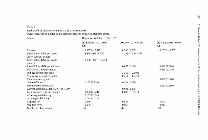
5.1. Replicating preÕious results

For our replication, we select three recent studies focused on the effect ofŽ .income inequality on aggregate saving, namely those by Sahota 1993 , Cook

Ž . Ž .1995 and Hong 1995 cited above. In each case, we maintain the authors’original specification, which in the first two studies involves the use of regional-dummy variables. Our data samples are somewhat smaller in country observationsthan the corresponding samples in the original studies because we limit ourselvesto the high-quality income and expenditure distribution data subset of Deiningerand Squire’s database, as discussed above. However, our data set is much larger inthe time dimension and includes more recent years.

Columns 1–3 in Table 3 present our attempt at replicating these authors’ resultsŽ .using the saving rate definition GDSrGDP adopted by them, and computing theŽ .individual country observations time averages over a time period as close as

possible to that in each original study. Our results in column 1, on a sample of 45OECD and developing countries, are very similar to Sahota’s: the parameterestimate on the Gini coefficient is positive and close to that reported by the authorŽ .0.19 , but well below conventional levels of significance. Regarding Cook’sspecification, applied to a sample of 28 LDCs, the effect of the Gini is also

Ž .positive but barely reaches a 10% confidence level column 2 . Finally, in Hong’sspecification, applied to 50 OECD and developing countries, the relevant distribu-tive variable is the income share of the top 20%, for which our results do replicatea positive effect significant at a 5% level.

As noted earlier, however, GDS and GDP are questionable measures of savingand income, and their use can be viewed as introducing measurement error in the

Ž .saving rate as well as the income level . In the sample, such measurement error,defined as the difference between the GDS and GNS ratios, is significantlypositively correlated with the inequality measures, which strongly suggests thattheir estimated coefficients in columns 1–3 of Table 3 are biased upward.11

Therefore, in columns 4–6 of Table 3, we redo the above estimations using GNSand GNP measures. The common finding across all three specifications is indeed adecline in the magnitude of the coefficient estimates on the inequality indicators,particularly in the case of Hong’s specification. Although their estimated standard

11 The correlation between this measurement error and the Gini coefficient equals 0.26 in the fullsample, and 0.45 for LDCs. Likewise, the correlation between the error and the top 20rbottom 40income share ratio equals 0.30. The other regressors are not significantly correlated with the differencebetween both saving ratios, with the exception of the growth rate, which shows a significant negativecorrelation — hence its coefficient estimates in columns 1–3 are likely biased downward.

()

K.Schm

idt-Hebbel,L

.SerÕenr

JournalofD

eÕelopm

entEconom

ics61

2000417

–446

´430

Table 3Ž .Replication of previous results t-statistics in parentheses

Note: t-statistics computed using heteroskedasticity-consistent standard errors.

Sample Dependent variable: GDSrGDP

Ž . Ž . Ž . Ž . Ž . Ž .1 Sahota 1972–1978 2 Cook 1970s LDCs 3 Hong 1965–1994full full

Ž . Ž . Ž .Constant y0.037 y0.417 0.208 1.035 y0.153 y0.735Ž . Ž .Real GDP or GNP per capita 4.47Ey05 5.206 4.24Ey05 4.757

Ž .1987 constant dollarŽ .Real GDP or GNP per capita y2.05Ey09 y4.537

squaredŽ . Ž .Real GDP or GNP growth rate 0.077 0.136 0.818 1.584

Ž . Ž .ln GDP or GNP per capita 0.030 2.728Ž .Old-age dependency ratio y3.365 y2.594Ž .Young-age dependency ratio y0.211 y0.470

Ž .Total dependency ratio 0.020 0.060Ž . Ž .Gini coefficient 0.182 0.938 0.384 1.736

Ž .Income share of top 20% 0.221 2.199Ž . Ž .Current account balancer GNP or GDP 0.601 2.838

Ž . Ž .Latin America regional dummy 0.088 2.044 y0.035 y1.516Ž .Africa regional dummy 0.153 3.391Ž .Asia regional dummy 0.131 4.771

2Adjusted R 0.369 0.556 0.401Standard error 0.059 0.057 0.047Number of observations 45 28 50

()

K.Schm

idt-Hebbel,L

.SerÕenr

JournalofD

eÕelopm

entEconom

ics61

2000417

–446

´431

Dependent variable: GNSrGNP

Ž . Ž . Ž . Ž . Ž . Ž . Ž . Ž . Ž . Ž .4 Sahota 1972–1978 full 5 Cook 1970s LDCs 6 Hong 1965–1994 full 7 Sahota 1965–1994 full 8 Cook 1965–1994 LDCs

Ž . Ž . Ž . Ž . Ž .0.025 0.249 0.020 0.120 0.157 0.767 0.048 0.681 0.197 1.128Ž . Ž . Ž . Ž .3.68Ey05 3.035 4.45Ey05 6.058 2.27Ey05 3.122 8.91Ey06 1.207Ž . Ž .y1.79Ey09 y2.947 y9.28Ey10 y2.578

Ž . Ž . Ž .0.589 1.592 1.421 4.187 0.626 1.749Ž .0.011 0.978

Ž . Ž .y1.789 y1.966 y0.624 y0.689Ž . Ž .0.213 0.589 y0.318 y0.806

Ž .0.088 0.895Ž . Ž . Ž . Ž .0.158 0.815 0.244 1.378 0.161 1.149 0.363 1.772

Ž .0.088 0.895Ž . Ž .0.695 4.995 0.667 2.866

Ž . Ž . Ž . Ž .0.031 0.577 y0.045 y2.876 0.007 0.181 y0.050 y3.110Ž . Ž .0.081 1.873 0.021 0.559Ž . Ž .0.088 2.363 0.081 2.509

0.233 0.638 0.511 0.355 0.3740.062 0.046 0.040 0.046 0.046

44 28 50 52 31


errors also decline slightly, the significance of the coefficient estimates falls wellbelow conventional levels.12

Next we expand the time dimension of the country averages by applyingSahota’s and Cook’s specifications to our longer 1965–1994 sample period. Thisallows us to add more countries to the sample, while still using GNS and GNP

Ž .measures. The results show that under Sahota’s specification column 7 the Ginicoefficient estimate remains virtually unaffected and statistically insignificant;

Ž .under Cook’s specification, it rises back to reach 10% significance column 8 .Ž .However, other robustness checks not reported to save space on Cook’s specifi-

cation show that dropping the Latin America dummy, whose inclusion seemsarbitrary, or the current account surplus — which, being the difference betweensaving and investment ratios, is clearly an endogenous variable — would makethe parameter estimate on the Gini coefficient considerably smaller and statisti-cally insignificant at any reasonable level.

We conclude that the basic finding of these three empirical studies — apositive effect of income concentration on aggregate saving — is not robust. In

Ž .two cases Hong’s and Sahota’s specifications , the result vanishes altogetherwhen using improved saving and income distribution measures, while in the third

Ž .one Cook’s equation it falls short of conventional significance levels and iscritically dependent on a questionable empirical specification. The natural questionis whether firmer evidence on the effect of income inequality on saving can befound using more standard specifications and testing for different samples andestimation techniques. This is our next topic.

5.2. Testing alternatiÕe specifications using cross-country data

We first examine the evidence from cross-country data, using country averagesfor the period 1965–1994. We start from a simple specification similar to those

Žfound in comparable cross-country studies of saving see, e.g., Schmidt-Hebbel et.al., 1992; Masson et al., 1995; Edwards, 1996 . It also encompasses the income,

Ž . Ž .demographic and inequality variables included by Sahota 1993 and Cook 1995 ;Žbut for the reasons already noted, exclude their more controversial variables the

12 One might argue that this discrepancy between the results based on GNS and GNP, and the earlierones obtained with GDS and GDP, could be due instead to errors of measurement of net income fromabroad, which would add random noise to the national saving rates. However, there are no clearreasons why net foreign transfers and factor payments, which are usually reflected in fairly reliablebalance-of-payments information, should be measured with less precision than domestic output.

Ž .Further, as noted in the text, the national income-based measures yield more precise albeit smallerparameter estimates than the domestic income-based ones, which seems to contradict such ‘‘random-noise’’ interpretation. Thus, we view as more plausible the alternative interpretation in the text thatGDS and GDP are noisy measures of the theoretically preferable GNS and GNP.


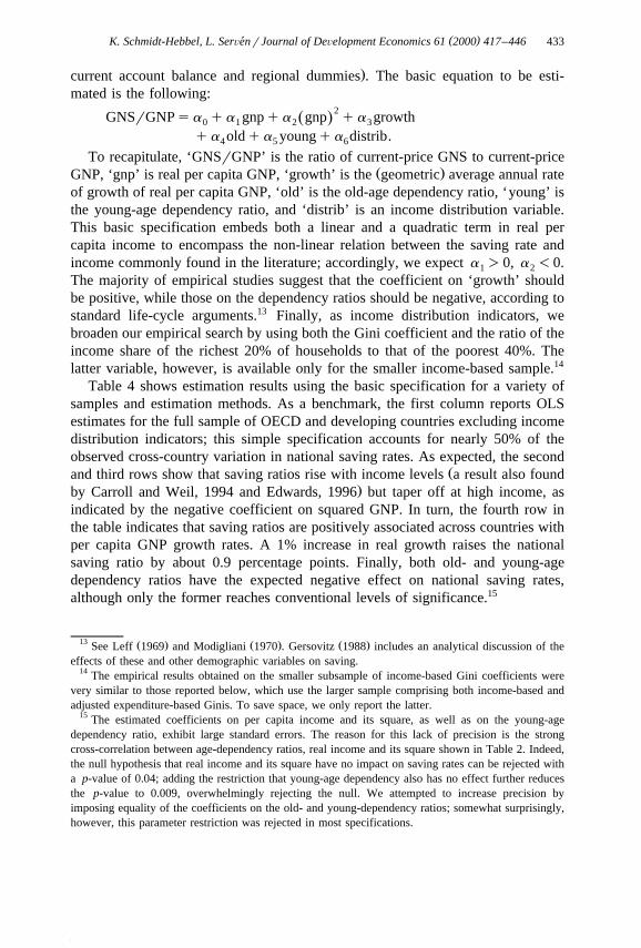
.current account balance and regional dummies . The basic equation to be esti-mated is the following:

2GNSrGNPsa qa gnpqa gnp qa growthŽ .0 1 2 3

qa oldqa youngqa distrib.4 5 6

To recapitulate, ‘GNSrGNP’ is the ratio of current-price GNS to current-priceŽ .GNP, ‘gnp’ is real per capita GNP, ‘growth’ is the geometric average annual rate

of growth of real per capita GNP, ‘old’ is the old-age dependency ratio, ‘young’ isthe young-age dependency ratio, and ‘distrib’ is an income distribution variable.This basic specification embeds both a linear and a quadratic term in real percapita income to encompass the non-linear relation between the saving rate andincome commonly found in the literature; accordingly, we expect a )0, a -0.1 2

The majority of empirical studies suggest that the coefficient on ‘growth’ shouldbe positive, while those on the dependency ratios should be negative, according tostandard life-cycle arguments.13 Finally, as income distribution indicators, webroaden our empirical search by using both the Gini coefficient and the ratio of theincome share of the richest 20% of households to that of the poorest 40%. Thelatter variable, however, is available only for the smaller income-based sample.14

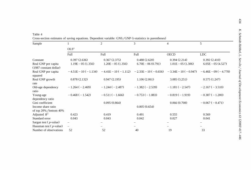
Table 4 shows estimation results using the basic specification for a variety ofsamples and estimation methods. As a benchmark, the first column reports OLSestimates for the full sample of OECD and developing countries excluding incomedistribution indicators; this simple specification accounts for nearly 50% of theobserved cross-country variation in national saving rates. As expected, the second

Žand third rows show that saving ratios rise with income levels a result also found.by Carroll and Weil, 1994 and Edwards, 1996 but taper off at high income, as

indicated by the negative coefficient on squared GNP. In turn, the fourth row inthe table indicates that saving ratios are positively associated across countries withper capita GNP growth rates. A 1% increase in real growth raises the nationalsaving ratio by about 0.9 percentage points. Finally, both old- and young-agedependency ratios have the expected negative effect on national saving rates,although only the former reaches conventional levels of significance.15

13 Ž . Ž . Ž .See Leff 1969 and Modigliani 1970 . Gersovitz 1988 includes an analytical discussion of theeffects of these and other demographic variables on saving.

14 The empirical results obtained on the smaller subsample of income-based Gini coefficients werevery similar to those reported below, which use the larger sample comprising both income-based andadjusted expenditure-based Ginis. To save space, we only report the latter.

15 The estimated coefficients on per capita income and its square, as well as on the young-agedependency ratio, exhibit large standard errors. The reason for this lack of precision is the strongcross-correlation between age-dependency ratios, real income and its square shown in Table 2. Indeed,the null hypothesis that real income and its square have no impact on saving rates can be rejected witha p-value of 0.04; adding the restriction that young-age dependency also has no effect further reducesthe p-value to 0.009, overwhelmingly rejecting the null. We attempted to increase precision byimposing equality of the coefficients on the old- and young-dependency ratios; somewhat surprisingly,however, this parameter restriction was rejected in most specifications.

()

K.Schm

idt-Hebbel,L

.SerÕenr

JournalofD

eÕelopm

entEconom

ics61

2000417

–446

´434

Table 4Ž .Cross-section estimates of saving equations. Dependent variable: GNSrGNP t-statistics in parentheses

Sample 1 2 3 4 5aOLS

Full Full Full OECD LDC

Ž . Ž . Ž . Ž . Ž .Constant 0.397 2.636 0.367 2.375 0.488 2.620 0.394 2.214 0.392 2.410Ž . Ž . Ž . Ž . Ž .Real GNP per capita 1.19Ey05 1.356 1.20Ey05 1.356 6.70Ey06 0.791 1.01Ey05 1.306 6.05Ey05 4.527

Ž .1987 constant dollarŽ . Ž . Ž . Ž . Ž .Real GNP per capita y4.51Ey10 y1.134 y4.41Ey10 y1.112 y2.33Ey10 y0.656 y3.34Ey10 y0.947 y6.46Ey09 y4.778

squaredŽ . Ž . Ž . Ž . Ž .Real GNP growth 0.878 2.132 0.947 2.195 1.106 2.061 3.085 3.251 0.575 1.247

rateŽ . Ž . Ž . Ž . Ž .Old-age dependency y1.264 y2.469 y1.244 y2.487 y1.382 y2.539 y1.181 y2.547 y2.167 y3.510

ratioŽ . Ž . Ž . Ž . Ž .Young-age y0.468 y1.542 y0.511 y1.666 y0.753 y1.883 y0.819 y1.919 y0.387 y1.200

dependency ratioŽ . Ž . Ž .Gini coefficient 0.095 0.864 0.066 0.708 y0.067 y0.471

Ž .Income share ratio 0.005 0.654of top 20%rbottom 40%

2Adjusted R 0.423 0.419 0.491 0.555 0.569Standard error 0.043 0.043 0.042 0.027 0.041

Ž .Sargan test p-value – – – – –Ž .Hausman test p-value – – – – –

Number of observations 52 52 40 19 33

()

K.Schm

idt-Hebbel,L

.SerÕenr

JournalofD

eÕelopm

entEconom

ics61

2000417

–446

´435

6 7 8 9aGMM Trimean

Full Full Full Full

Ž . Ž . Ž . Ž .y0.008 y0.029 y0.089 y0.244 0.332 2.094 0.631 3.930Ž . Ž . Ž . Ž .2.79Ey05 2.813 3.40Ey05 2.236 8.70Ey06 1.397 y5.00Ey06 y0.079Ž . Ž . Ž . Ž .y1.16Ey09 y2.596 y1.22Ey09 y2.097 y2.65Ey10 y0.874 1.09Ey10 0.369

Ž . Ž . Ž . Ž .2.463 2.687 2.537 2.966 1.307 3.225 1.162 2.953Ž . Ž . Ž . Ž .y0.233 y0.315 y0.554 y0.757 y1.066 y2.091 y1.736 y3.492Ž . Ž . Ž . Ž .0.402 0.713 0.337 0.426 y0.492 y1.577 y1.089 y3.241Ž . Ž .y0.113 y0.499 0.127 1.184

Ž . Ž .0.011 0.934 0.008 1.383– – – –

0.048 0.048 – –0.527 0.759 – –0.596 0.988 – –

47 39 52 40

a Ž .t-Statistics computed using heteroskedasticity-consistent standard errors. The equations using the top 20% to bottom 40% ratio columns 3, 7 and 9 as therelevant distribution measure were estimated using only observations with income-based distribution data.


Columns 2–3 in Table 4 add the income distribution indicators. The signpattern of the parameter estimates of the conventional variables remains un-changed, and their magnitude is rather similar to that in column 1. However,

Ž .neither the Gini coefficient column 2 nor the ratio of income shares of the topŽ .20% and bottom 40% of the population column 3 carry a significant coefficient.

Columns 4–5 split the sample between industrial and developing countries, usingthe Gini coefficient as inequality indicator. The resulting estimates suggest that thesaving–income and saving–growth relationships are not robust across country

Ž .groups. The saving–income link is weak among industrial countries column 4Ž .but very strong among developing countries column 5 , while the opposite applies

to the saving–growth relationship which appears strong among OECD countriesbut weak among LDCs — the same cross-country pattern found by Carroll and

Ž .Weil 1994 . The influence of demographic dependency on saving is negative inboth groups, although it varies in size and statistical significance. Finally, theparameter estimate of the Gini coefficient is positive for the OECD subsample andnegative for LDCs — the same sign pattern of the simple correlation mentionedearlier — but in both cases insignificantly different from zero. Interestingly,

Ž .estimates not reported on the two subsamples using the ratio of income sharesinstead of the Gini as inequality indicator yield the same sign pattern and lack ofsignificance.

One potential source of bias in these regressions is the possible endogeneity ofright-hand side variables. The level, growth rate, and distribution of income are alldetermined jointly with the saving rate, and reverse causality from the lattervariable to the rest is quite possible — for example, through the conventionalsaving–investment–output link mentioned earlier. In order to address this possiblesimultaneous equation bias, columns 6 and 7 of Table 4 report generalized method

Ž .of moments GMM estimates on the full country sample, using instruments forthe level, square, growth rate, and distribution of income.16

As the table shows, the sign pattern of the GMM estimates is similar to that ofthe OLS estimates. However, the coefficients of the instrumented GNP-relatedvariables are more than double in size relative to their OLS counterparts, and theyall become significant. This contrasts with the loss in precision of the coefficients

Ž .of the dependency ratios assumed exogenous . Finally, and most important, thetwo income distribution measures remain insignificant. The Sargan statisticspresented in the table reveal no evidence against the validity of the instruments. Asa more formal comparison between the GMM and the OLS estimates, we

16 The instruments used were the following: initial per-capita GNP and its square; population growth;years of schooling; secondary enrollment rate; black market premium; terms of trade shocks; initial life

Žexpectancy; political instability; and civil liberties. All of these variables except for the first two from. Ž .World Bank data were taken from Barro and Lee 1994 . Unavailability of data on some of the

Ž .instruments led to the loss of five observations in the full sample one in the income-based sample .


computed Hausman statistics testing the endogeneity of the income level and itssquare, growth rate, and distribution indicator. As can be seen from the table, thestatistics show very little evidence against the OLS estimates — although thismight be partly due to the low power of the Hausman test.

Heteroskedasticity and extreme observations are common problems in cross-country empirical studies, and while the point estimates and standard errors just

Ždiscussed remain consistent in the presence of heteroskedasticity and, further-.more, the GMM estimates remain asymptotically efficient , their accuracy in small

samples can be severely distorted in the presence of outlying observations. Thus,as a further check on our results, we computed robust estimators based onregression quintiles, still using our basic empirical specification. In columns 8–9of Table 4, we present estimation results using the trimean — a linear combina-

Ž .tion of the regression median or LAD estimator and the 25th and 75th quintiles,with weights 0.5, 0.25 and 0.25, respectively — which outperforms the OLS

Žestimator in the presence of even modest outlier contamination see Koenker and. 17Bassett, 1978 for evidence . Most parameter estimates are in fact very similar to

those obtained from OLS, and the income inequality indicators carry positive signsbut remain insignificant. However, the specification using the ratio of income

Ž .shares as inequality indicator column 9 shows a reversed sign pattern in theper-capita GNP polynomial.

Overall, the above results indicate that neither simultaneity nor outlyingobservations are the cause of our failure to find significant effects of incomeinequality on aggregate saving. In view of this fact, we experimented with anumber of other OLS specifications, using alternative income inequality measures,adding other saving regressors found in previous studies, and allowing fornonlinear effects of the income distribution indicators. The regression resultsŽ .Table 5 did not yield significant coefficients for the income inequality measuresin any of these alternative specifications.

To summarize, our extensive empirical tests on cross-section data find littleevidence of income inequality affecting aggregate saving. It might be argued,however, that these results are based on inefficient estimators, because we haveignored the time-series dimension of the data. Further, the fact that in previousstudies ad-hoc regional dummies seem to affect the significance of the inequalityindicators suggests that like in other cross-country empirical work, countryheterogeneity could be a potential problem in the regressions. The best way toaddress these concerns is by exploiting the full panel dimension of our data.

17 The LAD estimator itself, which in general is superior to the trimean under extreme outliercontamination, but inferior in less-extreme cases, yielded virtually identical results. In both cases, thecovariance matrix of the estimator was computed along the lines described by Koenker and BassettŽ .1982 .


Tab

le5

Ž.

Alt

erna

tive

OL

Ssp

ecif

icat

ions

.D

epen

dent

vari

able

:G

NS

rG

NP

t-st

atis

tics

inpa

rent

hese

sN

ote:

The

abov

et-

stat

isti

csw

ere

com

pute

dus

ing

hete

rosk

edas

tici

ty-c

orre

cted

stan

dard

erro

rs.

Sam

ple

12

34

56

Ful

lF

ull

Ful

lF

ull

Ful

lF

ull

Ž.

Ž.

Ž.

Ž.

Ž.

Ž.

Con

stan

t0.

6037

2.93

30.

394

2.00

90.

361

2.23

60.

189

0.95

40.

266

1.78

40.

302

1.87

4Ž

.Ž

.Ž

.Ž

.Ž

.Ž

.R

eal

GN

P9.

59E

y06

1.16

18.

90E

y06

1.07

51.

39E

y05

1.30

11.

26E

y05

1.36

41.

10E

y05

1.37

91.

48E

y05

1.83

8pe

rca

pita

Ž 198

7co

nsta

nt.

doll

arŽ

.Ž

.Ž

.Ž

.Ž

.Ž

.R

eal

GN

Ppe

ry

3.39

Ey

10y

0.99

6y

3.22

Ey

10y

0.93

5y

4.64

Ey

10y

1.25

2y

4.61

Ey

10y

1.11

8y

4.50

Ey

10y

1.21

6y

5.66

Ey

10y

1.53

9ca

pita

squa

red

Ž.

Ž.

Ž.

Ž.

Ž.

Ž.

Rea

lG

NP

1.15

42.

154

1.17

12.

182

0.95

82.

109

0.96

32.

283

0.94

12.

409

0.57

21.

224

grow

thra

teŽ

.Ž

.Ž

.Ž

.Ž

.Ž

.O

ld-a

gey

1.32

8y

2.46

3y

1.31

6y

2.43

0y

1.25

8y

2.59

3y

1.15

4y

2.34

0y

0.78

7y

1.47

6y

1.10

7y

2.07

0de

pend

ency

rati

oŽ

.Ž

.Ž

.Ž

.Ž

.Ž

.Y

oung

-age

y0.

741

y1.

968

y0.

770

y2.

025

y0.

512

y1.

662

y0.

474

y1.

530

y0.

315

y0.

999

y0.

551

y1.

771

depe

nden

cyra

tio

Ž.

Ž.

Ž.

Ž.

Gin

ico

effi

cien

t0.

112

0.66

70.

863

1.61

00.

154

1.21

30.

249

1.79

2Ž

.In

com

esh

are

y0.

250

y1.

257

ofm

iddl

e60

%Ž

.In

com

esh

are

0.21

931.

312

ofto

p20

%U

Ž.

GN

PG

ini

y4.

37E

y06

y0.

193

coef

fici

ent

Ž.

Gin

ico

effi

cien

ty

0.90

2y

1.40

0sq

uare

dŽ

.C

urre

ntac

coun

tr0.

561

2.44

3ba

lanc

eG

NP

Ž.

Lat

inA

mer

ica

y0.

016

y0.

428

regi

onal

dum

my

Ž.

Afr

ica

regi

onal

0.00

50.

143

dum

my

Ž.

Asi

are

gion

al0.

038

1.09

0du

mm

y2

Adj

uste

dR

0.50

80.

512

0.40

60.

417

0.41

10.

463

Sta

ndar

der

ror

0.04

10.

041

0.04

40.

043

0.04

20.

042

Num

ber

of40

4052

5248

52ob

serv

atio

ns


5.3. Panel data results

Table 6 reports unbalanced-panel regressions using 5-year averages for OECDand developing countries, jointly and separately. In all cases, the regressionsinclude a full set of time dummies that were jointly significant in most cases andhence retained for ease of comparison across estimations. The first column reportssimple pooled OLS estimates on the full sample, using our basic specification. Theresults are qualitatively similar to the cross-section OLS estimates, although themagnitude of the coefficients of the income level and growth variables isconsiderably smaller. In any case, the estimated impact of the Gini index remainssmall and insignificant. Analogous results were obtained using instead the ratio ofincome shares.

Column 2 adds regional dummies to the regression, thus reproducing the crudeŽ .attempt of previous studies to capture regional heterogeneity. While the dummies

Žthemselves are insignificant individually and jointly a test of their joint signifi-cance yields a p-value of 0.130, implying that they could be safely dropped from

.the regression , their addition does raise considerably the estimated parameter onthe Gini coefficient, which becomes significant at the 10% level.

This result confirms the need to control more satisfactorily for country hetero-geneity likely present in the data. To do so, in columns 3–6 in Table 6, wecompute fixed-effect panel estimates; this, however, removes from the sample 27developing countries possessing only one 5-year observation. Column 3 reportsfull-sample estimates using the Gini coefficient as distribution indicator. Compari-son with the preceding column reveals that the addition of country effects, with

Žthemselves as highly significant a Wald test of their joint significance yields a.p-value below 0.001 , greatly improves the overall precision of the estimates. The

clear exception is the Gini coefficient, whose point estimate is now close to zeroand insignificant.

These estimates also allow us to test whether the regional dummies capturesatisfactorily the country heterogeneity present in the sample. This amounts to

Ž .testing a set of linear restrictions specifically, 51 of them on the estimatedcountry dummies from column 3. The computed Wald statistic yielded a marginalsignificance level below 0.001, rejecting overwhelmingly the regional-dummy infavor of the fixed-effect specification.

Column 4 is analogous to column 3 but uses the ratio of the income share of thetop 20% to the bottom 40% of the population as the relevant income inequalitymeasure — which results in the loss of another 14 countries from the sample.While for the conventional regressors the results are fairly similar to the earlierones; the income inequality variable now carries a negative coefficient, statisticallysignificant at the 5% level.

Columns 5–6 report fixed effect estimates using the industrial and developingcountry subsamples, respectively, with the Gini coefficient as inequality indicator.For the former sample, the results are rather poor, as only the income growth rate


Tab

le6

Ž.

Pan

eles

tim

ates

ofsa

ving

equa

tion

s.D

epen

dent

vari

able

:G

NS

rG

NP

t-st

atis

tics

inpa

rent

hese

s

Est

imat

ion

proc

edur

e1

23

45

67

8

aa

aS

ampl

eP

oole

dO

LS

Fix

edef

fect

sP

anel

GM

M

Ful

lF

ull

Ful

lF

ull

OE

CD

LD

Cs

Ful

lF

ull

Con

stan

t0.

545

0.46

7N

AN

AN

AN

A0.

408

0.32

4Ž

.Ž

.Ž

.Ž

.6.

968

5.03

31.

540

2.67

2R

eal

GN

Ppe

rca

pita

4.23

Ey

066.

76E

y5

2.51

Ey

051.

64E

y05

4.14

Ey

066.

56E

y05

2.85

Ey

051.

33E

y05

Ž.

Ž.

Ž.

Ž.

Ž.

Ž.

Ž.

Ž.

1.00

51.

244

2.35

71.

742

0.54

92.

704

2.04

00.

989

Rea

lG

NP

per

capi

tasq

uare

dy

5.27

Ey

11y

1.40

Ey

10y

5.94

Ey

10y

3.33

Ey

106.

00E

y09

y3.

29E

y09

y8.

75E

y10

y2.

98E

y10

Ž.

Ž.

Ž.

Ž.

Ž.

Ž.

Ž.

Ž.

y0.

276

y0.

595

y2.

087

y1.

342

0.28

6y

2.00

4y

1.84

0y

0.57

0R

eal

GN

Pgr

owth

rate

0.50

90.

511

0.49

10.

474

0.32

70.

500

0.69

61.

838

Ž.

Ž.

Ž.

Ž.

Ž.

Ž.

Ž.

Ž.

2.22

12.

379

4.22

75.

695

2.49

53.

196

1.84

22.

777

Old

-age

depe

nden

cyra

tio

y1.

744

y1.

627

y2.

918

y2.

801

0.26

7y

3.58

y2.

486

y1.

341

Ž.

Ž.

Ž.

Ž.

Ž.

Ž.

Ž.

Ž.

y6.

507

y4.

801

y3.

164

y3.

236

0.47

2y

1.80

4y

4.02

7y

1.77

5Y

oung

-age

depe

nden

cyra

tio

y0.

91y

0.84

0y

0.57

3y

1.10

7y

0.25

7y

0.28

4y

0.58

6y

0.46

1Ž

.Ž

.Ž

.Ž

.Ž

.Ž

.Ž

.Ž

.y

5.98

6y

5.50

3y

1.73

7y

5.07

3y

1.31

2y

0.66

6y

1.68

6y

1.88

1G

ini

coef

fici

ent

0.05

40.

154

0.04

20.

119

0.07

00.

146

Ž.

Ž.

Ž.

Ž.

Ž.

Ž.

0.73

91.

897

0.34

81.

642

0.47

50.

452

Inco

me

shar

era

tio

ofy

0.00

90.

012

Ž.

Ž.

top

20%

rbo

ttom

40%

y2.

013

1.03

8L

atin

Am

eric

ay

0.02

1Ž

.re

gion

aldu

mm

yy

0.50

9A

fric

are

gion

aldu

mm

yy

0.00

6Ž

.y

0.14

7A

sia

regi

onal

dum

my

0.01

7Ž

.0.

482

Wal

dte

stof

join

t0.

000

0.00

00.

000

0.00

00.

000

0.00

00.

000

0.00

0Ž

.si

gnif

ican

cep-

valu

eŽ

.T

ime

effe

cts

p-va

lue

0.01

50.

027

0.30

50.

031

0.00

00.

399

0.45

10.

009

Sta

ndar

der

ror

0.07

10.

070

0.03

70.

030

0.06

00.

041

0.05

60.

046

Ž.

Sar

gan

test

p-va

lue

––

––

––

0.09

70.

591

2nd

orde

rau

toco

rrel

atio

n–

––

––

–0.

301

0.11

6Ž

.p-

valu

eŽ

.Ž

.Ž

.Ž

.Ž

.Ž

.Ž

.Ž

.N

umbe

rof

obse

rvat

ions

248

8224

882

221

5515

740

8619

135

3612

436

107

32Ž

.co

untr

ies

at-

Sta

tist

ics

com

pute

dus

ing

hete

rosk

edas

tici

ty-c

onsi

sten

tst

anda

rder

rors

.


Žis found significant, while the old-age dependency ratio carries a positive albeit.insignificant coefficient. The developing-country results are much more precise,

with the GNP-related variables carrying significant coefficients of the expectedsign. In both subsamples, and especially in the OECD, the parameter estimates onthe Gini coefficient increase somewhat relative to the full-sample estimate, but

Ž .remain below conventional significance levels. Similar results not reported wereobtained using the ratio of income shares as inequality indicator.

These panel data experiments clearly reject the regional-dummy specification asa satisfactory device to control for heterogeneity, but yield no evidence of anysystematic impact of inequality on saving. Thus, as a final check, we return to theissue of simultaneity in the panel context, to re-assess if endogeneity of theregressors might be the cause of the latter result. Under adequate assumptions,panel data allow the use of ‘‘internal’’ instruments to correct for simultaneityŽ .Arellano and Bond, 1991 . Following a GMM procedure recently proposed by

Ž .Blundell and Bond 1997 , we reestimate our basic equation using a systemframework that combines the original specification in levels with its first-dif-ferenced version.18

Columns 7 and 8 of Table 6 report the resulting full-sample GMM estimates.The estimation procedure summarized above requires at least three observationsper country on each variable, and this unfortunately leads to a considerable declinein sample size. Regarding the conventional regressors, the GMM estimates follow

Žthe already-familiar pattern. In the specification using the Gini coefficient column.7 , parameter estimates are fairly precise, with the clear exception of the Gini

itself, whose coefficient rises somewhat in magnitude but remains thoroughlyinsignificant. Interestingly, the time effects are insignificant as well, and otherexperiments reveal that dropping them would reverse the sign of the Ginicoefficient estimate, although the parameter would remain insignificant. In turn,

Ž .the regression including the ratio of income shares column 8 is somewhat lessprecise, and the inequality variable itself is also insignificant. The Sargan statisticstesting the validity of the instruments show some moderate evidence against thenull for the specification using the Gini, which suggests some caution regarding

18 We assume that the per-capita income level and growth variables, as well as the relevant incomedistribution indicator, are all endogenous; the demographic indicators are assumed exogenous. We useonce-lagged differences of the endogenous variables as additional instruments in the level specification,and twice-lagged levels of the endogenous variables as additional instruments in the first-differencedspecification. Validity of the latter instruments requires only that the residual of the first-differencedequation displays no autocorrelation of higher than first order, while validity of the former instruments

Ž .requires in addition that the correlation if any between the country-specific effect and the regressorsŽ .be time-invariant see Blundell and Bond, 1997 for further details . These assumptions can be assessed

empirically using Sargan-type and residual autocorrelation tests, as done here.


the GMM results, although the residual autocorrelation tests reveal no evidence ofmisspecification.

This concludes our comprehensive empirical search for the influence of incomeinequality on aggregate saving, controlling for other saving determinants. On thewhole, we find little evidence that income concentration has any systematic impacton aggregate saving. Only exceptionally have we found significant effects —

Ž .although of opposing signs: a positive one barely significant when using ad-hocŽregional dummies alone or in combination with another highly suspect variable,

.the current account deficit , and a negative one in some panel data subsampleswhen controlling for country-specific effects and using the ratio of income sharesas the relevant inequality measure.

6. Concluding remarks

The historical growth literature and more recent neoclassical consumptiontheory point out various channels through which income inequality affects per-

Ž .sonal saving. Most of these mechanisms but not all suggest positive direct effectsof income inequality on overall personal saving. However, recent political-econ-

Žomy research brings out negative indirect links from inequality through invest-.ment, growth, and public saving to aggregate saving. Taken together, these two

strands of the theoretical literature imply that the overall impact of inequality onaggregate saving is ambiguous and can be assessed only empirically.

The empirical literature based on household data typically finds a positiverelation between personal income inequality and overall personal saving. In turn,

Ž .some empirical studies based on macro national accounts saving data, typicallyconducted on cross-country samples, also report positive effects of personalincome inequality on aggregate saving. Other studies, however, find the oppositeresult or no effect whatsoever. Reconciling these conflicting results is difficultbecause macro-based empirical studies use widely different samples and specifica-tions, different measures of saving and inequality and in most cases incomedistribution information of questionable quality.

This paper has reexamined the empirical evidence from macro data on the linksbetween the distribution of personal income and aggregate saving, controlling forrelevant saving determinants, providing an encompassing framework and a robust-ness check for previous empirical studies, and extending them in five dimensions:Ž . Ž .i testing alternative saving specifications; ii using alternative inequality and

Ž . Ž .saving measures; iii making use of newer, better, and larger databases; ivconducting estimations jointly and separately for industrialized and developing

Ž .countries; and v applying various estimation techniques on both cross-countryand panel data. On the whole, we do not find any consistent effect of incomeinequality on aggregate saving — a result that agrees with the theoreticalambiguity.


Acknowledgements

We are grateful to Klaus Deininger and Lyn Squire for kindly making availableto us their database on income distribution. We thank Aart Kraay, Steve Marglin,Branko Milanovic, Vito Tanzi, and two anonymous referees for useful commentsand suggestions on an earlier version. Excellent research assistance by WanhongHu and Faruk Khan is gratefully acknowledged.

Appendix A

Ž .Deininger and Squire’s 1996 cross-country time-series database on annualincome inequality measures embodies major improvements over existing databases.A clear distinction is made between income- and expenditure-based inequalitymeasures, as well as between household- and individual-based, and the underlyingprimary data are checked for important quality criteria: they have to be based on

Ž .household or individual surveys not on national accounts , their coverage has toŽ .be comprehensive i.e., based on nation-wide samples , and measurement of

Ž . Žincome or expenditure has to be comprehensive as well including all income or.expenditure categories .

While the total number of country-year observations in Deininger–Squire is2621, applying the three latter quality criteria reduces the number to 682 high-qu-ality country-year observations, corresponding to 108 countries and years withinthe period 1890–1995. For these observations, both Gini coefficients and incomeshares by population quintiles are available. Of the latter 682 observations, we

Žinclude in our subsample only those 468 country-year observations corresponding. Žto 82 countries that fall into the 1965–1994 period the one for which we have

.complete macroeconomic data . However, this set includes observations based onincome data along with others based on expenditure data. We made the Ginicoefficients from income- and expenditure-based data comparable by followingthe procedure described in Section 4.

For the cross-country sample, averages over 1960–1994 were used for thefollowing variables: GDSrGDP ratio, real GDP per capita, and growth rate of realGDP per capita. For all other variables, averages over 1965–1994 were used,except where indicated otherwise. An additional requirement is imposed on thecross-country sample to achieve a minimum of time representation: countries areincluded only if they have at least one observation in each of the following two15-year periods: 1965–1979 and 1980–1994. This leaves us with 52 country

Ž .observations 19 industrial and 33 developing economies for the income- andŽexpenditure-based subsample and 40 country observations 17 industrial and 23

.developing economies for the income-based subsample.The panel data sample comprises 5-year country averages. Unlike with the

cross-country data, we expand our data set to include all countries regardless of


the number of 5-year periods for which they possess observations. The number ofŽ .5-year country observations for income distribution variables Table 1 is 270

Ž . Ž .178 for income- and expenditure-based data income-based data . The number ofŽ .observations used in the panel regressions Table 6 is lower because of missing

data on some of the regression variables. Eighty-two countries are included in thefull panel sample, of which, 20 are industrial and 62 are developing countries.

Variable definitions and sources are summarized next.Variable Definition and SourceGNS ratio GNSrGNP ratio, each series in current prices and local

currency. Source: World Bank National AccountsŽ .WBNA

GDS ratio GDSrGDP ratio, each series in current prices and localcurrency. Source: WBNA

Real GNP per capita In constant 1987 US dollars. Source: WBNAReal GDP per capita In constant 1987 US dollars. Source: WBNAGrowth rate of real Annual growth rate computed from real GNP per capitaGNP per capitaGrowth rate of real Annual growth rate computed from real GDP per capitaGDP per capita

Ž .Gini coefficient Source: Deininger and Squire 1996Ž .Ratio of income share Source: Deininger and Squire 1996

of top 20% to bottom40% of population andincome share ofmiddle 60%

Ž . Ž .Old age and young age Population aged 65 and over 14 and below as share ofdependency ratio total population. Source: World Bank Social Indicators

References

Alesina, A., Perotti, R., 1996. Income distribution, political instability, and investment. EuropeanEconomic Review 40, 1203–1228.

Alesina, A., Rodrik, D., 1994. Distributive politics and economic growth. Quarterly Journal ofEconomics 109, 465–490.

Arellano, M., Bond, S., 1991. Some tests of specification for panel data: Monte Carlo evidence and anapplication to employment equations. Review of Economic Studies 58, 277–297.

Barro, R., Lee, L., 1994. Data set for a panel of 138 countries, http:rrwww.nber.org.rbarro.lee,January.

Becker, G., 1975. Human Capital. NBER, Cambridge.Blinder, A., 1975. Distribution effects and the aggregate consumption function. Journal of Political

Economy 87, 608–626.Blundell, R., Bond, S., 1997. Initial conditions and moment restrictions in panel data models.

University College London Discussion Paper 97-07.


Bosworth, B.P., 1993. Saving and Investment in a Global Economy. Brookings, Washington, DC.Bunting, D., 1991. Savings and the distribution of income. Journal of Post Keynesian Economics 14,

3–22.Carroll, C., 1997. Buffer-stock saving and the life-cyclerpermanent income hypothesis. Quarterly

Ž .Journal of Economics CXII 1 , 1–56.Ž .Carroll, C., 1998. Why do the rich save so much? In: Slemrod, J. Ed. , Does Atlas Shrug? Economic

Consequences of Taxing the Rich. Cambridge Univ. Press, London.Ž .Carroll, C., Kimball, M., 1996. On the concavity of the consumption function. Econometrica 64 4 ,

981–992.Carroll, C., Weil, D., 1994. Saving and growth: a reinterpretation. Carnegie–Rochester Conference

Series on Public Policy 40, 133–192.Clarke, G., 1992. More evidence on income distribution and growth. Policy Research Working Paper

1064, The World Bank.Collins, S., 1991. Saving behavior in ten developing countries. In: Bernheim, B.D., Shoven, J.B.

Ž .Eds. , National Saving and Economic Performance. University of Chicago Press, Chicago, pp.349–372.

Cook, C., 1995. Saving rates and income distribution: further evidence from LDCs. Applied Economics27, 71–82.

Cowell, F., 1977. Measuring Inequality: Techniques for the Social Sciences. Wiley, New York.Deaton, A., 1991. Saving and liquidity constraints. Econometrica 59, 1121–1142.Deaton, A., 1992. Understanding Consumption. Clarendon Press, Oxford.

Ž .Deaton, A., 1999. Saving and growth. In: Schmidt-Hebbel, K., Serven, L. Eds. , Understanding´Consumption. Clarendon Press, Oxford.

Deininger, K., Squire, L., 1996. A new data set measuring income inequality. World Bank EconomicReview 10, 565–591.

Della Valle, P., Oguchi, N., 1976. Distribution, the aggregate consumption function, and the level ofeconomic development: some cross-country results. Journal of Political Economy 84, 1325–1334.

Dornbusch, R., Edwards, S., 1991. The macroeconomics of populism. In: Dornbusch, R., Edwards, S.Ž .Eds. , The Macroeconomics of Populism in Latin America. University of Chicago Press, Chicago.

Dynan, K., Skinner, J., Zeldes, S., 1996. Do the rich save more? Unpublished manuscript.Edwards, S., 1996. Why are Latin America’s saving rates so low? An international comparative

Ž .analysis. Journal of Development Economics 51 1 , 5–44.Ž .Gersovitz, M., 1988. Saving and development. In: Chenery, H., Srinivasan, T.N. Eds. , Handbook of

Development Economics. North-Holland, Amsterdam.Gupta, K., 1970. Personal saving in developing nations: further evidence. Economic Record 46,

243–249.Hong, K., 1995. Income distribution and aggregate saving, unpublished manuscript. Harvard Univer-

sity, Cambridge, MA, November.Houthakker, H., 1961. An international comparison of personal saving. Bulletin of the International

Statistical Institute 38, 55–69.Kaldor, N., 1957. A model of economic growth. Economic Journal 57.Kelley, A.C., Williamson, J.G., 1968. Household savings behavior in developing countries: the

Ž .Indonesian case. Economic Development and Cultural Change 16 3 , 385–403.Kirman, A., 1992. Whom or what does the representative individual represent? Journal of Economic

Perspectives 2, 117–136.Koenker, R., Bassett, G., 1978. Regression quantiles. Econometrica 46, 33–50.Koenker, R., Bassett, G., 1982. Robust tests for heteroskedasticity based on regression quantiles.

Econometrica 50, 43–61.Kotlikoff, L., Summers, L., 1981. The role of intergenerational transfers in aggregate capital accumula-

tion. Journal of Political Economy 90, 706–732.Kotlikoff, L., Summers, L., 1988. The contribution of intergenerational transfers to total wealth: a


Ž .reply. In: Kessler, D., Masson, A. Eds. , Modeling the Accumulation and Distribution of Wealth.Clarendon Press, Oxford.

Leff, N.H., 1969. Dependency rates and savings rates. American Economic Review 59, 886–896.Levine, R., Renelt, D., 1992. A sensitivity analysis of cross-country growth regressions. American

Economic Review 82, 942–963.Lewis, W.A., 1954. Economic development with unlimited supplies of labor. The Manchester School

22, 139–191.Lim, D., 1980. Income distribution, export instability and savings behavior. Economic Development

and Cultural Change 26, 359–364.Maddison, A., 1992. A long-run perspective on saving. Scandinavian Journal of Economics 94,

181–196.Mankiw, N., Romer, D., Weil, D., 1992. A contribution to the empirics of economic growth. Quarterly

Journal of Economics 107, 407–438.Mas-Colell, A., Whinston, M., Green, J., 1995. Microeconomic Theory. Oxford Univ. Press, Oxford.Masson, P., Bayoumi, T., Samiel, H., 1995. Saving behavior in industrial and developing countries,

International Monetary Fund, Staff Studies for the World Economic Outlook. International Mone-tary Fund, September.

Menchik, P., David, M., 1983. Income distribution, lifetime savings, and bequests. American EconomicReview 73, 672–690.

Modigliani, F., 1970. The life-cycle hypothesis of savings and intercountry differences in the savingsŽ .ratio. In: Eltis, W.A., Scott, M.F.G., Wolfe, J.N. Eds. , Induction, Growth and Trade. Oxford

Univ. Press, Oxford.Musgrove, P., 1980. Income distribution and the aggregate consumption function. Journal of Political

Economy 88, 504–525.Ogaki, M., Ostry, J., Reinhart, C.M., 1996. Saving behavior in low- and middle-income developing

countries: a comparison. IMF Staff Papers 43, pp. 38–71.Pasinetti, L., 1962. Rate of profit and income distribution in relation to the rate of economic growth.

Review of Economic Studies 29, 267–279.Perotti, R., 1996. Growth, income distribution, and democracy: what the data say. Journal of Economic

Growth 1, 149–187.Persson, T., Tabellini, G., 1994. Is inequality harmful for growth? Theory and evidence. American

Economic Review 84, 600–621.Ž .Sahota, G., 1993. Saving and distribution. In: Gapinski, J.H. Ed. , The Economics of Saving. Kluwer

Academic Publishers, Boston.Ž .Schmidt-Hebbel, K., Serven, L. Eds. , The Economics of Saving and Growth. Cambridge Univ. Press,´

London.Schmidt-Hebbel, K., Serven, L., Solimano, A., 1996. Saving and investment: paradigms, puzzles,´

policies. World Bank Research Observer 11, 87–117.Schmidt-Hebbel, K., Webb, S., Corsetti, G., 1992. Household saving in developing countries: first

cross-country evidence. World Bank Economic Review 6, 529–547.Solow, R., 1956. A contribution to the theory of economic growth. Quarterly Journal of Economics 70,

65–94.Venieris, Y., Gupta, D., 1986. Income distribution and sociopolitical instability as determinants of

savings: a cross-sectional model. Journal of Political Economy 94, 873–883.Williamson, J., 1968. Personal saving in developing nations: an intertemporal cross-section from Asia.

Economic Record 44, 194–202.

Does income inequality raise aggregate...

Documents

Transcript of Does income inequality raise aggregate...