Does everyone have an override code?

Project 1 due Friday 9pm

Review of Filtering

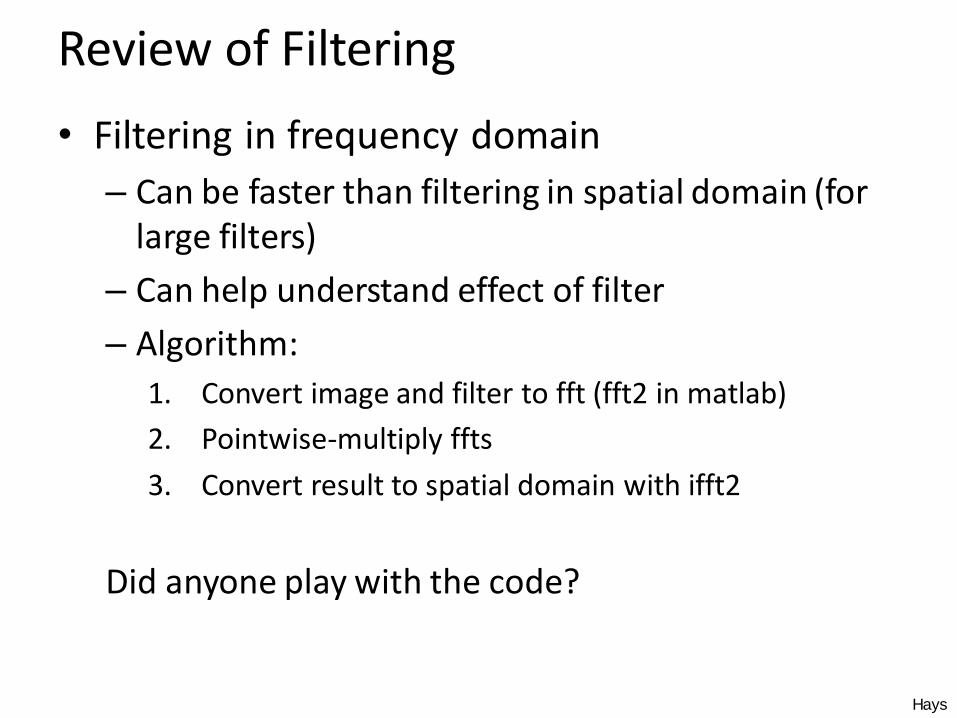
• Filtering in frequency domain

– Can be faster than filtering in spatial domain (for large filters)

– Can help understand effect of filter

– Algorithm:

1. Convert image and filter to fft (fft2 in matlab)

2. Pointwise-multiply ffts

3. Convert result to spatial domain with ifft2

Did anyone play with the code?

Hays

Review of Filtering

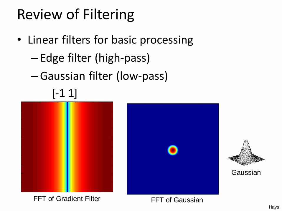
• Linear filters for basic processing

– Edge filter (high-pass)

– Gaussian filter (low-pass)

FFT of Gaussian

[-1 1]

FFT of Gradient Filter

Gaussian

Hays

More Useful Filters

1st Derivative of Gaussian

(Laplacian of Gaussian)

Earl F. Glynn

Things to Remember

• Sometimes it makes sense to think of images and filtering in the frequency domain– Fourier analysis

• Can be faster to filter using FFT for large images• N logN vs. N2 for auto-correlation

• Images are mostly smooth– Basis for compression

• Remember to low-pass before sampling• Otherwise you create aliasing

Hays

Aliasing and Moiré patterns

Gong 96, 1932, Claude Tousignant, Musée des Beaux-Arts de Montréal

http://blogs.discovermagazine.com/badastronomy/2009/06/24/the-blue-and-the-green/

The blue and green colors are actually the same

Why do we get different, distance-dependent interpretations of hybrid images?

?

Hays

• Early processing in humans filters for orientations and scales of frequency.

Early Visual Processing: Multi-scale edge and blob filters

Clues from Human Perception

Campbell-Robson contrast sensitivity curve

Perceptual cues in the mid-high

frequencies dominate perception.

Frequency increase (log)

Con

trast

decre

ase (

log

)

Application: Hybrid Images

• A. Oliva, A. Torralba, P.G. Schyns, “Hybrid Images,” SIGGRAPH 2006

When we see an image from far away, we

are effectively subsampling it!

How is it that a 4MP image can be compressed to a few hundred KB without a noticeable change?

Thinking in Frequency - Compression

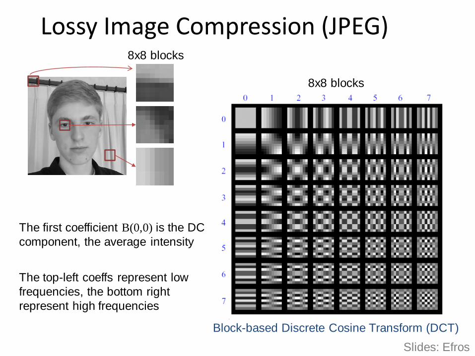
Lossy Image Compression (JPEG)

Block-based Discrete Cosine Transform (DCT)

Slides: Efros

The first coefficient B(0,0) is the DC

component, the average intensity

The top-left coeffs represent low

frequencies, the bottom right

represent high frequencies

8x8 blocks

8x8 blocks

Image compression using DCT

• Compute DCT filter responses in each 8x8 block

• Quantize to integer (div. by magic number; round)

– More coarsely for high frequencies (which also tend to have smaller values)

– Many quantized high frequency values will be zero

Quantization divisers (element-wise)

Filter responses

Quantized values

JPEG Encoding

• Entropy coding (Huffman-variant)Quantized values

Linearize B

like this.Helps compression:

- We throw away

the high

frequencies (‘0’).

- The zig zag

pattern increases

in frequency

space, so long

runs of zeros.

Color spaces: YCbCr

Y(Cb=0.5,Cr=0.5)

Cb(Y=0.5,Cr=0.5)

Cr(Y=0.5,Cb=05)

Y=0 Y=0.5

Y=1Cb

Cr

Fast to compute, good for

compression, used by TV

James Hays

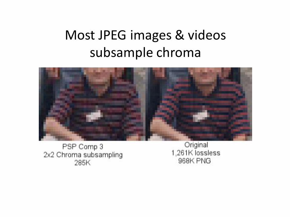
Most JPEG images & videos subsample chroma

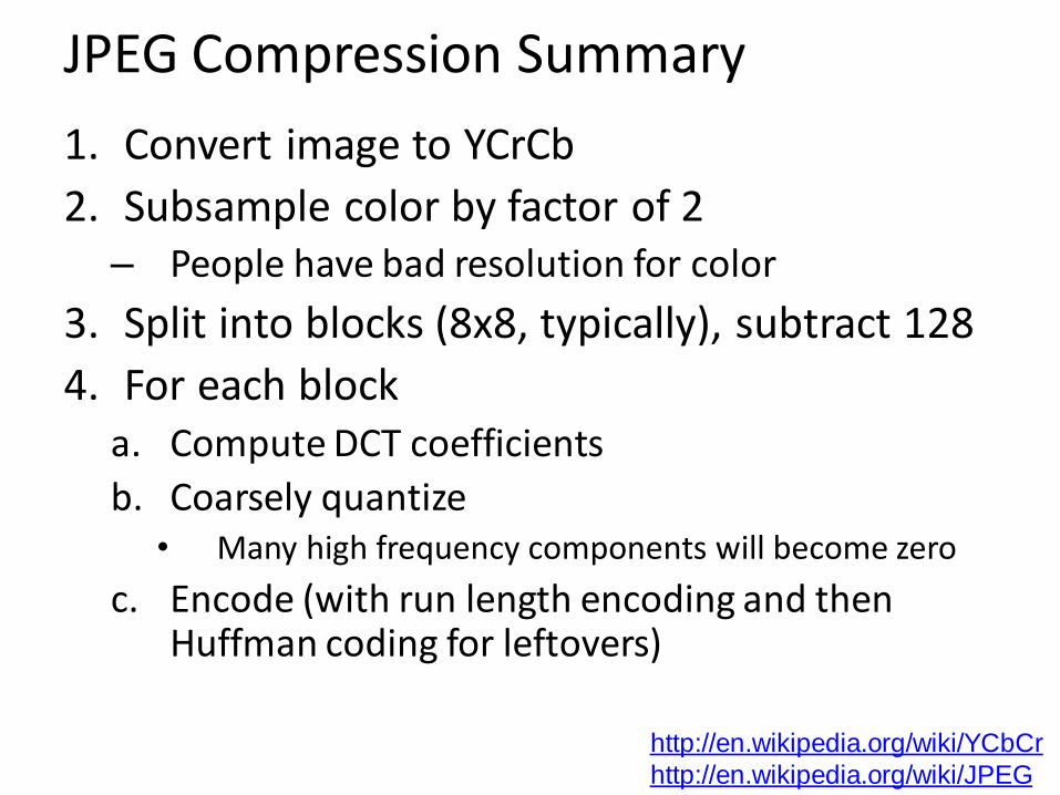
JPEG Compression Summary

1. Convert image to YCrCb

2. Subsample color by factor of 2– People have bad resolution for color

3. Split into blocks (8x8, typically), subtract 128

4. For each blocka. Compute DCT coefficients

b. Coarsely quantize• Many high frequency components will become zero

c. Encode (with run length encoding and then Huffman coding for leftovers)

http://en.wikipedia.org/wiki/YCbCr

http://en.wikipedia.org/wiki/JPEG

EDGE / BOUNDARY DETECTION

Many slides from James Hays, Lana Lazebnik, Steve Seitz, David Forsyth, David Lowe, Fei-Fei Li, and Derek Hoiem

Szeliski 4.2

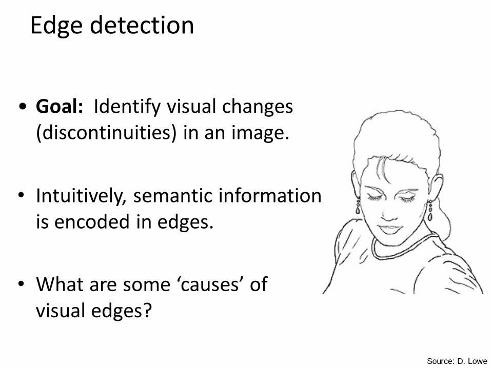
Edge detection

• Goal: Identify visual changes (discontinuities) in an image.

• Intuitively, semantic information is encoded in edges.

• What are some ‘causes’ ofvisual edges?

Source: D. Lowe

Origin of Edges

• Edges are caused by a variety of factors

depth discontinuity

surface color discontinuity

illumination discontinuity

surface normal discontinuity

Source: Steve Seitz

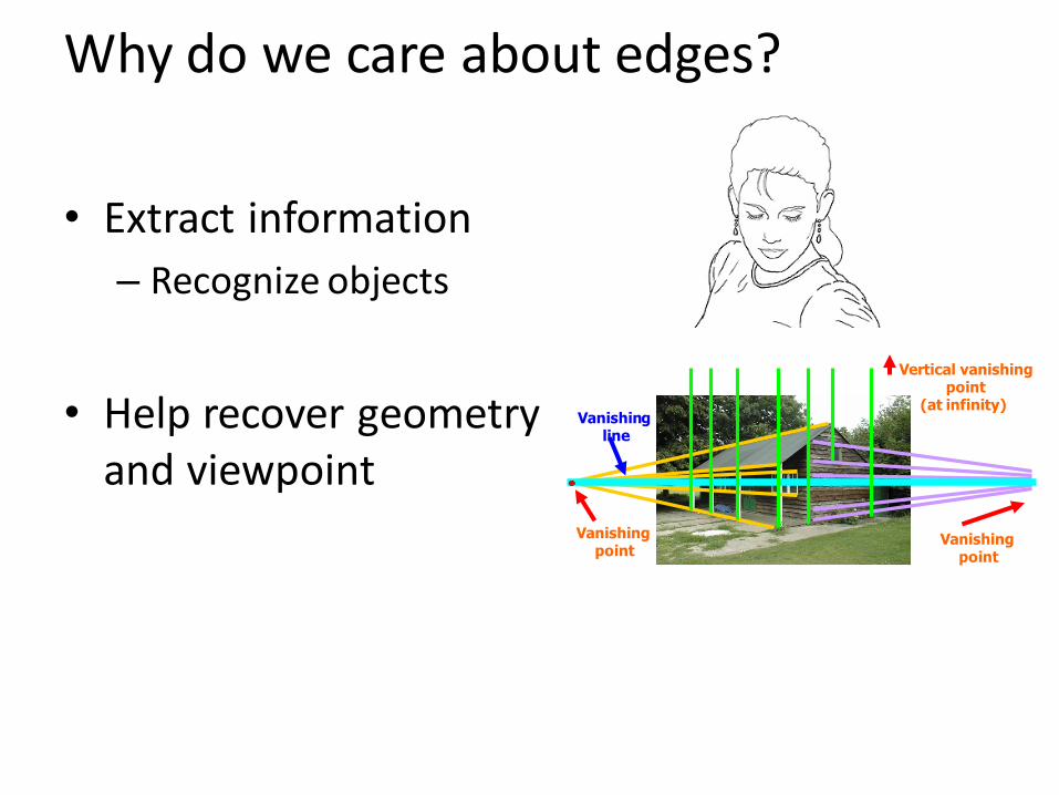
Why do we care about edges?

• Extract information

– Recognize objects

• Help recover geometry and viewpoint

Vanishingpoint

Vanishingline

Vanishingpoint

Vertical vanishingpoint

(at infinity)

Closeup of edges

Source: D. Hoiem

Closeup of edges

Source: D. Hoiem

Closeup of edges

Source: D. Hoiem

Closeup of edges

Source: D. Hoiem

Characterizing edges

• An edge is a place of rapid change in the image intensity function

imageintensity function

(along horizontal scanline) first derivative

edges correspond to

extrema of derivative

Hays

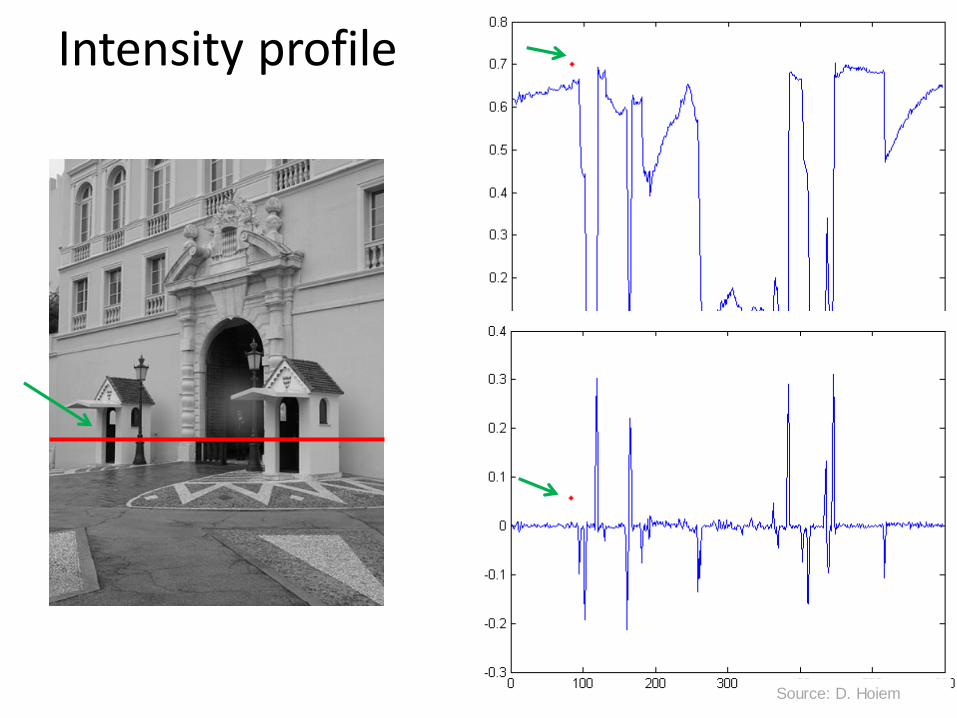
Intensity profile

Source: D. Hoiem

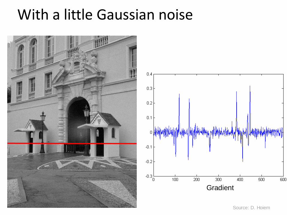
With a little Gaussian noise

Gradient

Source: D. Hoiem

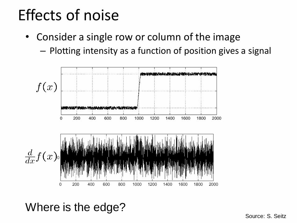
Effects of noise• Consider a single row or column of the image

– Plotting intensity as a function of position gives a signal

Where is the edge?Source: S. Seitz

Effects of noise

• Difference filters respond strongly to noise

– Image noise results in pixels that look very different from their neighbors

– Generally, the larger the noise the stronger the response

• What can we do about it?

Source: D. Forsyth

Solution: smooth first

• To find edges, look for peaks in )( gfdx

d

f

g

f * g

)( gfdx

d

Source: S. Seitz

• Differentiation is convolution, and convolution is associative:

• This saves us one operation:

gdx

dfgf

dx

d )(

Derivative theorem of convolution

gdx

df

f

gdx

d

Source: S. Seitz

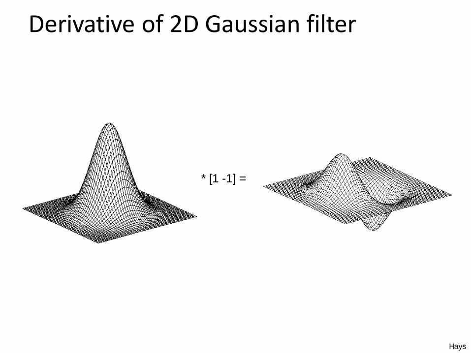
Derivative of 2D Gaussian filter

* [1 -1] =

Hays

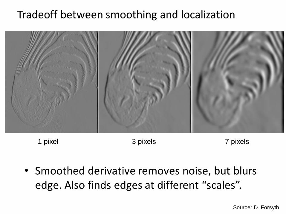
• Smoothed derivative removes noise, but blurs edge. Also finds edges at different “scales”.

1 pixel 3 pixels 7 pixels

Tradeoff between smoothing and localization

Source: D. Forsyth

Think-Pair-Share

• What is a good edge detector?

• Do we lose information when we look at edges? Are edges ‘incomplete’ as a representation of images?

Designing an edge detector• Criteria for a good edge detector:

– Good detection: the optimal detector should find all real edges, ignoring noise or other artifacts

– Good localization• the edges detected must be as close as possible to

the true edges• the detector must return one point only for each

true edge point

• Cues of edge detection– Differences in color, intensity, or texture across the

boundary– Continuity and closure– High-level knowledge

Source: L. Fei-Fei

Designing an edge detector

• “All real edges”

• We can aim to differentiate later on which edges are ‘useful’ for our applications.

• If we can’t find all things which could be called an edge, we don’t have that choice.

• Is this possible?

Closeup of edges

Source: D. Hoiem

Elder – Are Edges Incomplete? 1999

What information would we need to

‘invert’ the edge detection process?

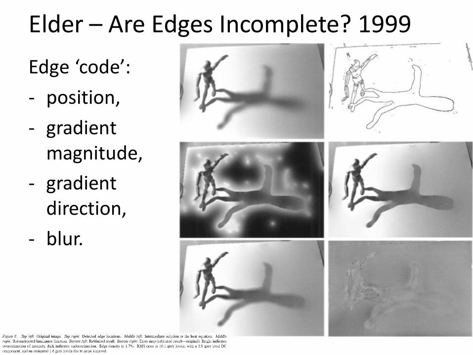
Elder – Are Edges Incomplete? 1999

Edge ‘code’:

- position,

- gradient magnitude,

- gradient direction,

- blur.

Where do humans see boundaries?

• Berkeley segmentation database:http://www.eecs.berkeley.edu/Research/Projects/CS/vision/grouping/segbench/

image human segmentation gradient magnitude

pB slides: Hays

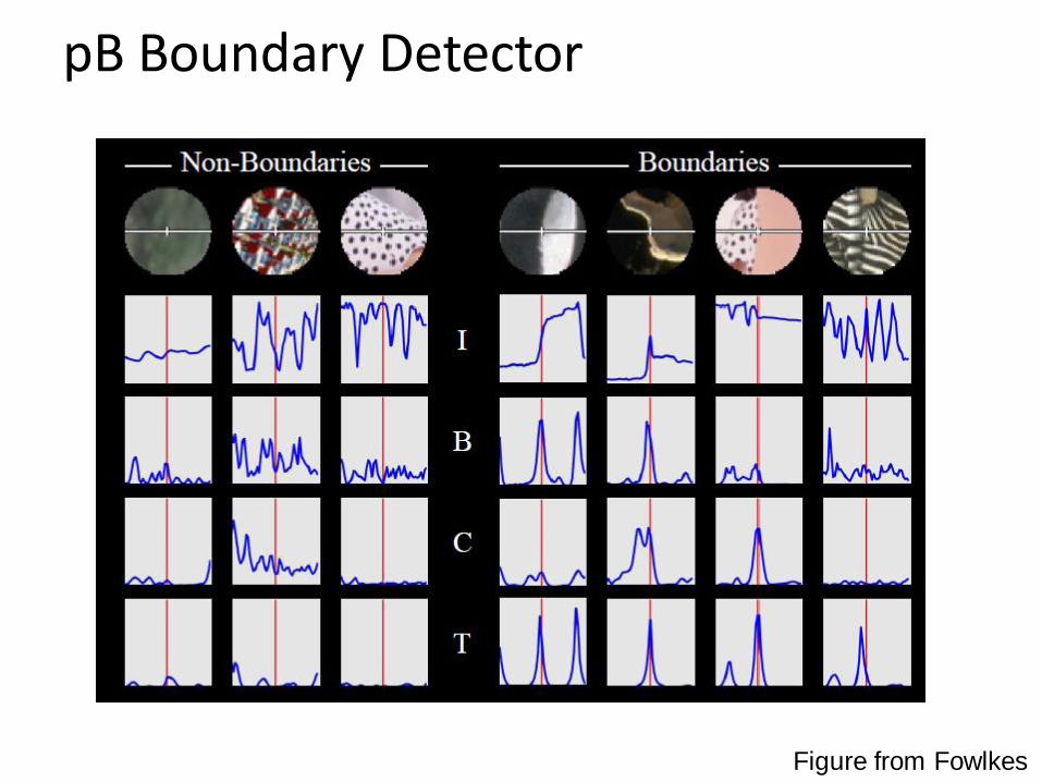
pB boundary detector

Figure from Fowlkes

Martin, Fowlkes, Malik 2004: Learning to Detect

Natural Boundaries…

http://www.eecs.berkeley.edu/Research/Projects/C

S/vision/grouping/papers/mfm-pami-boundary.pdf

Brightness

Color

Texture

Combined

Human

pB Boundary Detector

Figure from Fowlkes

Results

Human (0.95)

Pb (0.88)

Results

Human

Pb

Human (0.96)

Global PbPb (0.88)

Human (0.95)

Pb (0.63)

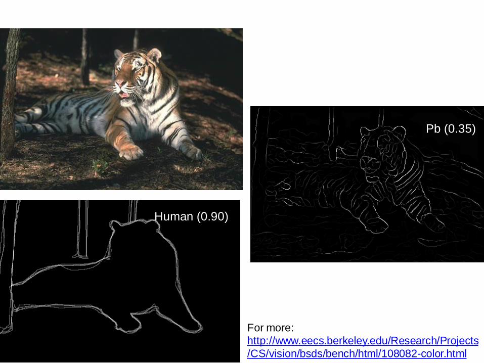
Human (0.90)

Pb (0.35)

For more:

http://www.eecs.berkeley.edu/Research/Projects

/CS/vision/bsds/bench/html/108082-color.html

45 years of boundary detection

Source: Arbelaez, Maire, Fowlkes, and Malik. TPAMI 2011 (pdf)

State of edge detection

• Local edge detection works well

– ‘False positives’ from illumination and texture edges (depends on our application).

• Some methods to take into account longer contours

• Modern methods that actually “learn” from data.

• Poor use of object and high-level information.

Hays

Wednesday

• Classic Canny edge detector – 22,000 citations

• Interest Points and Corners